Huntington Beach Shoreline ContaminationInvestigation, Phase III

Coastal Circulation and Tr ansport Patterns: The Likelihood of OCSD’ sPlume Impacting the Huntington Beach Shoreline

Executi ve Summary

Open-File Report 03-62

U.S. Department of the InteriorU.S. Geological Sur vey

Huntington Beach Shoreline Contamination Investigation, Phase III

C o a s t a l C i rc u l a t i o n a n d Tra n s p o rt P a t t e rn s : T h e L i ke l i h o o d o f O C S D ’ s P l u m e I m p a c t i n g t h e H u n t i n g t o n B e a c h , CA S h ore l i n e

EXECUTIVE SUMMARY

Open-File Report 03-622 0 0 3

B y

Marlene N o b l e

1, J i n g p i n g X u

1, L e s l i e R o s e n f e l d

2, J o h n Largier

3, Pe t e r H a m i l to n4,

B u r t J o n e s

5 , G e o r ge Robertson6

1 U. S . G e o l o g i c a l S u r vey, M e n l o Park , C A2 N a va l P o s t g r a d u a t e S c h o o l , M o nterey, C A3 S c r i p p s I n st i t u t i o n o f O c e a nog ra p h y, L a J o l l a , C A4 S c i e n t i f i c A p p l i c a t i o n I n t e r n a t i o n a l C o rpo ra t i o n , R a l e i g h , N C5 U n i ve r s i t y o f S o u t h e r n C a l i fo rn i a , L o s A n ge l e s , C A6 O ra n ge C o u n t y S a n i ta t i o n D i s t r i c t , Fo u n t a i n Va l l e y, C A

This report is preliminary and has not been rev i ewed for conformity with U.S. Geological Survey editorial standard orwith the North American Stratigraphic Code. A ny use of trade, product, or fi rm names is for descriptive purposes onlyand does not imply endorsement by the U.S. Gove rn m e n t .

ii

iii

TABLE OF CONTENTS

1. Background . . . . . . . . . . . . . . . . . . . . . . . . . . . . . . . . . . . . . . . . . . . . . . . . . . . . . . . . . . . . . . . . . . . . .1

2. Hypotheses . . . . . . . . . . . . . . . . . . . . . . . . . . . . . . . . . . . . . . . . . . . . . . . . . . . . . . . . . . . . . . . . . . . . . .3

3. Objectives and Methods . . . . . . . . . . . . . . . . . . . . . . . . . . . . . . . . . . . . . . . . . . . . . . . . . . . . . . . . . . . .5

4. Measurement Program . . . . . . . . . . . . . . . . . . . . . . . . . . . . . . . . . . . . . . . . . . . . . . . . . . . . . . . . . . . . .6

5. Major Findings . . . . . . . . . . . . . . . . . . . . . . . . . . . . . . . . . . . . . . . . . . . . . . . . . . . . . . . . . . . . . . . . . . .6

5.1. Surfzone Bacteria Contamination Patterns . . . . . . . . . . . . . . . . . . . . . . . . . . . . . . . . . . . . . . . . .6

5.1.1. Multi-year Patterns . . . . . . . . . . . . . . . . . . . . . . . . . . . . . . . . . . . . . . . . . . . . . . . . . . . . . . . .6

5.1.2. Summer 2001 Patterns . . . . . . . . . . . . . . . . . . . . . . . . . . . . . . . . . . . . . . . . . . . . . . . . . . . . .7

5.2. Outfall Plume Tracking . . . . . . . . . . . . . . . . . . . . . . . . . . . . . . . . . . . . . . . . . . . . . . . . . . . . . . .11

5.2.1. Spatial Patterns of the Plume . . . . . . . . . . . . . . . . . . . . . . . . . . . . . . . . . . . . . . . . . . . . . . .11

5.2.2. Bacteria Concentrations . . . . . . . . . . . . . . . . . . . . . . . . . . . . . . . . . . . . . . . . . . . . . . . . . . .14

5.3. Coastal Ocean Transport Processes . . . . . . . . . . . . . . . . . . . . . . . . . . . . . . . . . . . . . . . . . . . . . .15

5.3.1. Subtidal Transport . . . . . . . . . . . . . . . . . . . . . . . . . . . . . . . . . . . . . . . . . . . . . . . . . . . . . . .15

5.3.2. Diurnal and Semidiurnal Transport . . . . . . . . . . . . . . . . . . . . . . . . . . . . . . . . . . . . . . . . . .17

5.3.2.1. Seabreeze and Diurnal Currents . . . . . . . . . . . . . . . . . . . . . . . . . . . . . . . . . . . . . . . .17

5.3.2.2. Semidiurnal Currents . . . . . . . . . . . . . . . . . . . . . . . . . . . . . . . . . . . . . . . . . . . . . . . . .19

5.3.2.3. Cross-Shelf Transport Events in the Coastal Ocean . . . . . . . . . . . . . . . . . . . . . . . . .20

5.3.3. Nearshore Cross-Shore Transport . . . . . . . . . . . . . . . . . . . . . . . . . . . . . . . . . . . . . . . . . . .21

5.3.4. Resuspended Sediment Transport . . . . . . . . . . . . . . . . . . . . . . . . . . . . . . . . . . . . . . . . . . .24

6. Coastal Transport Processes and Their Relationship to Significant Bacterial Patterns . . . . . . . . . . .25

6.1. Subtidal Cross-Shelf Transport Pathways: Newport Canyon . . . . . . . . . . . . . . . . . . . . . . . . . . .25

6.2. Diurnal and Semidiurnal Transport Pathways . . . . . . . . . . . . . . . . . . . . . . . . . . . . . . . . . . . . . .27

6.3. Coastal Ocean Event Transport Pathways . . . . . . . . . . . . . . . . . . . . . . . . . . . . . . . . . . . . . . . . .27

6.4. Sediment Transport Pathways . . . . . . . . . . . . . . . . . . . . . . . . . . . . . . . . . . . . . . . . . . . . . . . . . .28

6.5. Nearshore Transport Pathways . . . . . . . . . . . . . . . . . . . . . . . . . . . . . . . . . . . . . . . . . . . . . . . . . .28

7. Conclusions . . . . . . . . . . . . . . . . . . . . . . . . . . . . . . . . . . . . . . . . . . . . . . . . . . . . . . . . . . . . . . . . . . . .29

8. References . . . . . . . . . . . . . . . . . . . . . . . . . . . . . . . . . . . . . . . . . . . . . . . . . . . . . . . . . . . . . . . . . . . . .30

Draft Final Report on attached CD

Huntington Beach Shoreline Contamination Investigation, Phase III

Coastal Circulation and Tr a n s p o rt Patterns: The Likelihood of OCSD’s Off s h o reWastewater Plume Impacting the Huntington Beach, CA Shore l i n e

TABLE OF CONTENTS

VOLUME I: Surfzone Sampling and Moored Obser vations

Chapter 1. Introduction and Background

Leslie Rosenfeld, Marlene Noble, Peter Hamilton, Burt Jones, John Largier, Jingping Xu

Chapter 2. Surfzone Bacteria Patterns

Leslie Rosenfeld

Chapter 3. Subtidal Circulation Pathways

Peter Hamilton

Chapter 4. Newport Canyon Transport Pathway

Kevin Orzech, Marlene Noble

Chapter 5. Seabreeze

Peter Hamilton

Chapter 6. Tidal Transport Pathways

Marlene Noble, Peter Hamilton

Chapter 7. Sediment Resuspension and Transport Pathway

Jingping Xu

Chapter 8. Near-shore Circulation Pathways

John Largier

Chapter 9. Methodology

Peter Hamilton, Burt Jones, John Largier,Marlene Noble, Leslie Rosenfeld, Jingping Xu

VOLUME II: Hydr ographic Sur veysBurt Jones

iv

Huntington BeachS h o reline Contamination Investigation, Phase III

Coastal Circulation and Tr a n s p o rt Patterns: The Likelihood of Orange County SanitationD i s t r i c t ’s Off s h o re Wastewater Plume Impacting the Huntington Beach, CA Shore l i n e

A B S T R AC T

A consortium of investigators have conducted an extensive investigation of the coastal ocean circulationand transport pathways off Huntington Beach, California with the aim of identifying any causal links thatmay exist between the offshore discharge of wastewater by Orange County Sanitation District (OCSD) andthe significant bacterial contamination observed along the Huntington Beach shoreline. This is the thirdstudy supported by OCSD to determine possible land-based and coastal ocean sources for the significantbacterial contamination levels measured during several summer periods off Huntington Beach.

Although the study identifies several possible coastal ocean pathways by which diluted wastewater maybe transported to the beach, including internal tide, sea-breeze and subtidal flow features, there were nodirect observations of either the high bacteria concentrations seen in the OCSD plume at the shelf breakreaching the shoreline in significant levels or of an association between the existence of a coastal oceanprocess and beach contamination at or above AB411 levels. It is concluded that the OCSD plume is not amajor cause of beach contamination; no causal links could be demonstrated. This conclusion is based onthe absence of direct observation of plume-beach links, on analysis of the spatial and temporal patterns ofshoreline contamination and coastal ocean processes, and on the observation of higher levels ofcontamination at the beach than in the plume.

1. BACKGROUND

The beaches off Huntington Beach, California (Figure 1) were closed or posted for several months inthe summers of 1999 and 2000 because bacteria levels in the swash zone exceeded beach sanitationstandards contained in California Health and Safety Code §115880 (Assembly Bill 411, Statutes of 1997,Chapter 765; AB411) for extended periods. Because these closures and postings occurred during the peakof summer seasons, they had a major impact on the local, recreational and business communities. Therewere a wide variety of studies conducted during Phase I (OCSD, 1999) and Phase II (Grant et al., 2000)of the Huntington Beach Shoreline Contamination Investigations, but specific sources for many of thecontamination events that caused beach closures and postings could not be determined. However, possiblecontamination pathways from upland sources, adjacent estuaries and the coastal ocean were identified. Inparticular, it was suggested that bacteria-rich effluent from the Orange County Sanitation District’s(OCSD) outfall plume might be brought to shore through several coastal ocean pathways. Bacteria fromthis effluent plume might then account for the contamination events observed along the Huntington Beachshoreline. To identify and evaluate potential coastal-ocean pathways, OCSD formed a Technical AdvisoryCommittee (TAC) to help design and oversee a Phase III study for the summer of 2001. The TAC formeda hypothesis ad-hoc committee consisting of regulators, research scientists, environmental groups andinterested citizens that formulated a series of potential transport mechanisms after considering historicalcontamination patterns, evaluating known coastal ocean processes and obtaining public comments todetermine processes that were most likely to contaminate the beach in summer.

1

2

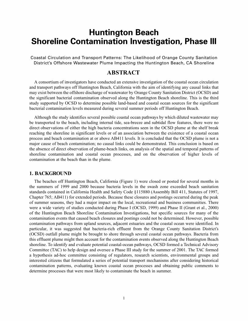
Figure 1a. Map of the region, the mooring sites and surfzone sampling stations. Sediment transport instrumentsare deployed at HB03, HB05, HB07, and HB11. The meteorological buoy is at HB07. Inset shows instrumentationsof a typical mooring.

2. HYPOTHESES

Field observations have shown, and plume models predict, that the OCSD effluent plume remainstrapped below the thermocline in the summer season (MEC final report, 2001) due to strong stratification.Hence, the primary hypothesis of this program was that coastal ocean processes that transport water andsuspended material below the thermocline have the greatest potential to transport the OCSD plume intothe nearshore region (water depths of 10-15 m (33-49 ft)) during the summer months. If the plume wascarried into the nearshore region, it was possible that local beaches were at risk of significant bacterialcontamination.

Internal tides

Internal tides are the most likely coastal-ocean process that could transport the submerged wastewaterplume into the nearshore regions. Once nearshore, other possible pathways could bring the water from thenearshore region into the surfzone. These nearshore pathways include:

3

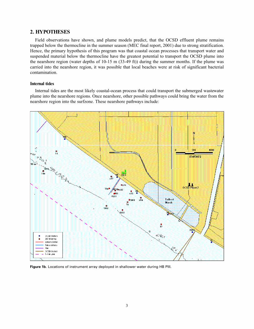
Figure 1b. Locations of instrument array deployed in shallower water during HB PIII.

a. If the effluent plume is transported into the nearshore region, it could enter the proximity of theAES Corporation power plant cooling water intake and discharge pipes and be entrained by theintake and/or discharge jet. Through either pathway, the effluent would then contaminate thethermal plume, which could easily be moved onshore through buoyant spreading, wind forcing orother processes.

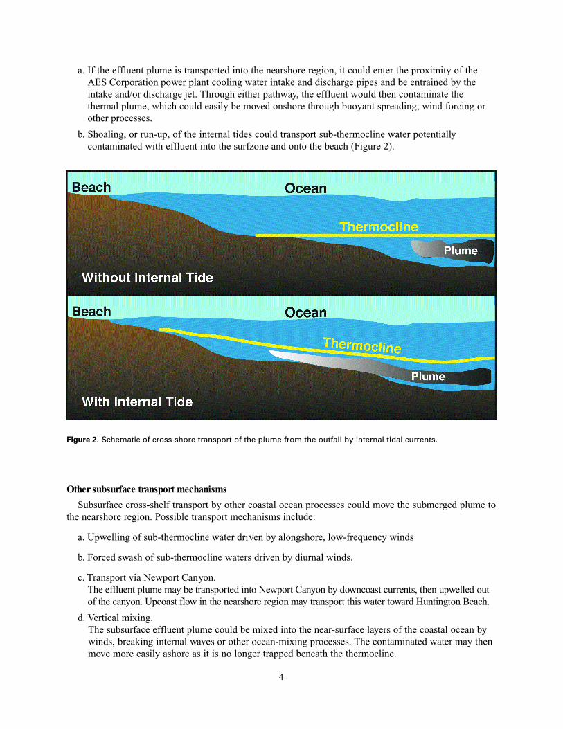
b. Shoaling, or run-up, of the internal tides could transport sub-thermocline water potentiallycontaminated with effluent into the surfzone and onto the beach (Figure 2).

Other subsurface transport mechanisms

Subsurface cross-shelf transport by other coastal ocean processes could move the submerged plume tothe nearshore region. Possible transport mechanisms include:

a. Upwelling of sub-thermocline water driven by alongshore, low-frequency winds

b. Forced swash of sub-thermocline waters driven by diurnal winds.

c. Transport via Newport Canyon. The effluent plume may be transported into New p o rt Canyon by downcoast currents, then upwelled outof the canyon. Upcoast flow in the nearshore region may transport this water toward Huntington Beach.

d. Vertical mixing.The subsurface effluent plume could be mixed into the near-surface layers of the coastal ocean bywinds, breaking internal waves or other ocean-mixing processes. The contaminated water may thenmove more easily ashore as it is no longer trapped beneath the thermocline.

4

Figure 2. Schematic of cross-shore transport of the plume from the outfall by internal tidal currents.

e. A combination of specific subtidal transport events.For example, if subtidal flows near the outfall are weak or stalled, the effluent would not be carriedas quickly as it is normally carried from the region. Hence, a larger volume of effluent is potentiallyavailable to be transported toward the beach.

Sediment transport processes

Particulate matter discharged by the OCSD outfall may settle out near the outfall and may contain highlevels of bacteria. Surface or internal waves could resuspend this bottom sediment and the particle-boundbacteria. Cross-shelf transport processes may then bring this material toward the shore. The researchprogram was designed to monitor this process, although the TAC ad-hoc committee thought that sediment-transport processes were not the most likely mechanism for transporting effluent bacteria to shore becausefine material normally moves from shallow to deeper water.

Buoyant particles

It is possible that buoyant particles (e.g., oil and grease) discharged at the outfall could reach the surfaceeven when the water column is stratified; bacteria may adhere to these particles. The TAC ad-hoccommittee discussed transport processes in the sea-surface microlayer, but did not think these processeswould account for either the high values or the spatial and temporal patterns of bacterial contamination ofthe beach. Monitoring data from OCSD have shown poor association (r2=0.08) between grease, oil andfecal coliform bacteria in the offshore region (SAIC and MEC, 1991). Shoreline microbiology samplinghas shown that the presence of grease particles on the beach is rare. Therefore, this element was notincluded as design criteria for either the hydrographic or moored sampling programs.

3. OBJECTIVES AND METHODS

The principle objective for this multi-faceted measurement program was to determine if there is a causallink between offshore wastewater discharge and significant bacterial contamination at or above state beachsanitation standards (i.e., AB411) along the Huntington Beach shoreline. This objective included the aimof identifying coastal ocean processes that could explain any observed links or that could provide insightto the possibility of shoreward transport of outfall plume waters. A secondary objective was to determinethe principal coastal-ocean circulation patterns in this region, which will allow for the evaluation of otherpotential contamination pathways suggested in the future. A final objective was to compare conditionsduring the summer of 2001 with those in 1999 and other years that have a high incidence of surfzonebacteria contamination.

In order to meet these objectives, data from moored arrays and hydrographic and beach surveys wereused to evaluate transport pathways or processes that could potentially bring the effluent plume from theouter shelf into the nearshore regions. The evaluation process consisted of three primary segments:

• Do the pathways or processes exist in the coastal ocean?What are the dominant characteristics of those pathways or processes?

• Can the pathways or processes transport material in the effluent plume to the nearshore region?

• Is there a causal association between identified coastal ocean processes or pathways andcontamination events that exceed AB411 standards in the surfzone?

– In the spatial surveys of effluent plume characteristics off Huntington Beach.

– In the spatial and temporal structure of coastal ocean circulation patterns determined from themoored array data.

5

4. MEASUREMENT PROGRAM

The measurement program consisted of: 1) a moored array that would collect data to provide a generaldescription and understanding of coastal circulation and mixing patterns, 2) a complementaryhydrographic mapping program that would provide a more detailed description of the spatial distributionof water column properties, and 3) a surfzone sampling program for bacteria.

Instrumented moorings at 12 locations monitored current velocity, temperature, and salinity at manydepths every few minutes for 4 months in the summer/fall of 2001 (Figure 1a). This deployment periodspans the time period when shoreline bacterial contamination has historically been at its maximum. Near-bottom wave, water-clarity and suspended sediments were collected at 4 sites to monitor sedimenttransport processes. Real-time meteorological data were collected at the shelf break. This array monitoredcoastal ocean transport processes with temporal frequencies ranging from a few minutes (e. g. internalwaves) to hours and days (e. g. internal tides and wind-driven processes) along 2 cross-shelf transportpathways and over a nearshore region next to Newport canyon. Additional moorings were deployed inwater depths less than 10 m from July to October 2001 to address transport pathways between thenearshore and the surfzone.

The principal moored array was designed by the US Geological Survey (USGS) and prepared anddeployed through a cooperative effort among the USGS, the Naval Postgraduate School (NPS) and ScienceApplications International Corporation (SAIC). The nearshore set of moorings was deployed by ScrippsInstitution of Oceanography (SIO) under contract with OCSD and MBC Applied Environmental Services(MBC) through a contract with the AES power plant.

A complementary hydrographic mapping program measured the spatial distribution of water columnproperties including temperature, salinity, ammonia, bacteria, and other properties of the water columnduring six surveys centered around periods of maximum tidal range (spring tides) (Figure 1a). Theseperiods were chosen because historical data indicated that most bacterial exceedances at the beachoccurred during spring tides (MEC, 2000). Five of the six surveys overlapped the moored arraydeployment. A series of CTD casts monitored water properties along 4 nearshore lines that run parallel tothe beach. Simultaneously, a towed undulating vehicle (TUV) monitored water column properties along 10offshore lines oriented approximately perpendicular to the beach. The hydrographic surveys were designedby OCSD, with advice from the University of Southern California (USC), and conducted by USC, MECAnalytical Systems, and OCSD.

Three types of fecal indicator bacteria (total coliform, fecal coliform and Enterococci) are collected inankle-depth water 5 days/week (including one weekend day) as part of OCSD’s standard beach monitoringplan. Samples are generally collected between 5 and 10 AM local time, with sampling proceeding from thenorthernmost station to the southernmost. During the six hydrographic surveys, additional microbiologysamples were collected hourly along the beach for 48 hours at the standard OCSD sampling sites (with theexception of the first cruise in May when the hourly sampling was done for only 36 hours).

5. MAJOR FINDINGS

5.1. Surfzone Bacterial Contamination Patterns

5.1.1. Multi-year Patterns

The total and fecal coliforms and Enterococci concentrations measured in the surfzone between 1 July 1998and 31 December 2001 were analyzed with respect to their temporal and spatial va r i a b i l i t y. The majority ofsamples have bacterial concentrations less than, or equal to, the minimum detection limit (58% of samples for

6

total coliform, 72% for fecal coliform, and 65% for Enterococci). Single sample bacteria concentrations we r ecompared to both the single sample (SS) and the geometric mean monthly (MM) AB411 standards:

Total coliform > 10,000 mpn / 100 ml (SS); 1,000 mpn / 100 ml (MM)Total coliform > 1000 mpn / 100 ml and Total coliform / fecal coliform < 10 (SS)Fecal coliform > 400 mpn / 100 ml (SS); 200 mpn / 100 ml (MM)Enterococci > 104 mpn / 100 ml (SS); 35 mpn / 100 ml (MM)

There are numerous exceedances of the AB411 single sample standards (3% of the samples for totalcoliform, 2% for fecal coliform and 6% for Enterococci). Here, the total coliform exceedances areconservatively defined as having values greater than 1000 mpn/100ml. The majority of those exceedancesare for Enterococci, as was found in previous studies (Grant et al. 2000). The percentage of samplesexceeding the AB411 standards is not significantly different for the HB Phase III period when comparedto the 1998-2001 period. Because of nighttime sampling, there was a slightly higher percentage of thesingle sample Enterococci concentrations with values greater than the allowable geometric monthly meanlevel in the summer of 2001 (22% vs. 17%).

The incidence of high concentrations of bacteria confirm a previously identified relationship with thelunar cycle (MEC, 2000; Grant et al., 2000), such that higher bacteria concentrations are associated withmaximum tidal ranges (i.e. spring tides). The larger the tidal range (or equivalently, the lower the dailylower low water, or the higher the daily higher high water), the higher the probability of a contaminationevent. It is interesting to note that in southern California, the timing of the largest spring tides relative tothe annual cycle changes very little from year to year. The phases of the diurnal and semidiurnal tidalconstituents are such that the largest spring tides fall in the summer (May-August) and winter (December-February). The larger of the two ebb tides (higher high water to lower low water) falls at night during thesummer spring tides, with the higher high tide at 8-10 PM local time.

5.1.2. Summer 2001 Patterns

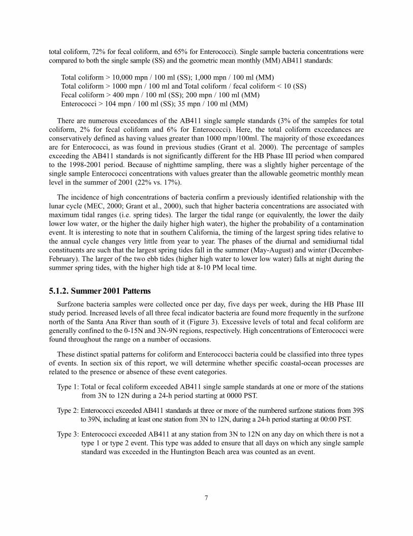
Surfzone bacteria samples were collected once per day, five days per week, during the HB Phase IIIstudy period. Increased levels of all three fecal indicator bacteria are found more frequently in the surfzonenorth of the Santa Ana River than south of it (Figure 3). Excessive levels of total and fecal coliform aregenerally confined to the 0-15N and 3N-9N regions, respectively. High concentrations of Enterococci werefound throughout the range on a number of occasions.

These distinct spatial patterns for coliform and Enterococci bacteria could be classified into three typesof events. In section six of this report, we will determine whether specific coastal-ocean processes arerelated to the presence or absence of these event categories.

Type 1: Total or fecal coliform exceeded AB411 single sample standards at one or more of the stationsfrom 3N to 12N during a 24-h period starting at 0000 PST.

Type 2: Enterococci exceeded AB411 standards at three or more of the numbered surfzone stations from 39Sto 39N, including at least one station from 3N to 12N, during a 24-h period starting at 00:00 PST.

Type 3: Enterococci exceeded AB411 at any station from 3N to 12N on any day on which there is not atype 1 or type 2 event. This type was added to ensure that all days on which any single samplestandard was exceeded in the Huntington Beach area was counted as an event.

7

8

F i g u re 3. L o g1 0 of total coliform, fecal coliform, and Enterococci concentration (mpn / 100 ml) are plotted versustime and distance alongshore. The data set subsampled to no more than daily values, was used. Black x's indicatethe day and location of each sample. AB411 single sample standards are indicated on the colorbars. Note the scaled i ff e rences on the colorbars.Data is contoured with PlotPlus on a 180 x 13 grid (time and distance, re s p e c t i v e l y )using cay=5 and nrng=2. The cay value determines the interpolation scheme. Cay=0 means Laplacian interpolationis used. As cay is increased, spline interpolation predominates over Laplacian. For pure spline interpolationc a y = i n f i n i t y. Grid points are set to "undefined", and not used, if farther than nrng away from the nearest data point.

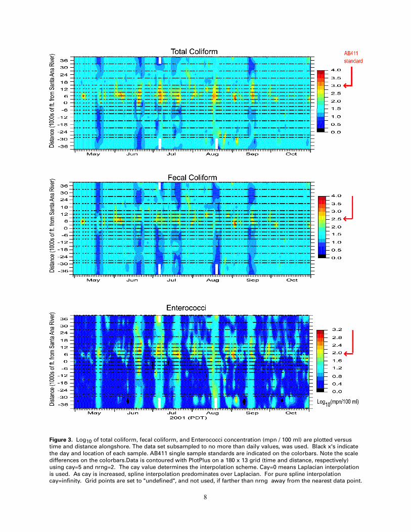
Almost every surfzone sample between 39S and 39N that exceeded an AB411 single sample standardduring the HB Phase III study fell on a day characterized as a type 1, 2, or 3 event (Figure 4). The sea leveldata confirm that contamination events tend to occur during spring tides.

9

Figure 4. The vertical bars indicate days on which bacterial events occurred, blue=type 1, magenta=type 2,gray=types 1 and 2, gold= type 3. Sea level measured at Los Angeles is shown at the bottom of the figure. A blackdot is plotted at each time (GMT) and location a sample was taken. Colored symbols are plotted at the time (GMT)and location of samples exceeding AB411 single sample standards. The size of the symbol is proportional to theratio of the measured bacterial concentration to the AB411 criteria. The symbol size for a sample equal to theAB411 criteria is shown to the right of the indicator species in the legend.

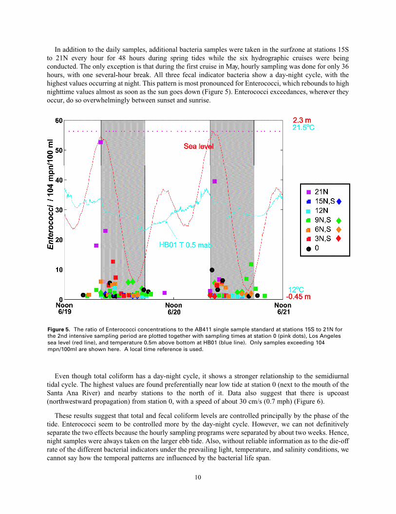
In addition to the daily samples, additional bacteria samples were taken in the surfzone at stations 15Sto 21N every hour for 48 hours during spring tides while the six hydrographic cruises were beingconducted. The only exception is that during the first cruise in May, hourly sampling was done for only 36hours, with one several-hour break. All three fecal indicator bacteria show a day-night cycle, with thehighest values occurring at night. This pattern is most pronounced for Enterococci, which rebounds to highnighttime values almost as soon as the sun goes down (Figure 5). Enterococci exceedances, wherever theyoccur, do so overwhelmingly between sunset and sunrise.

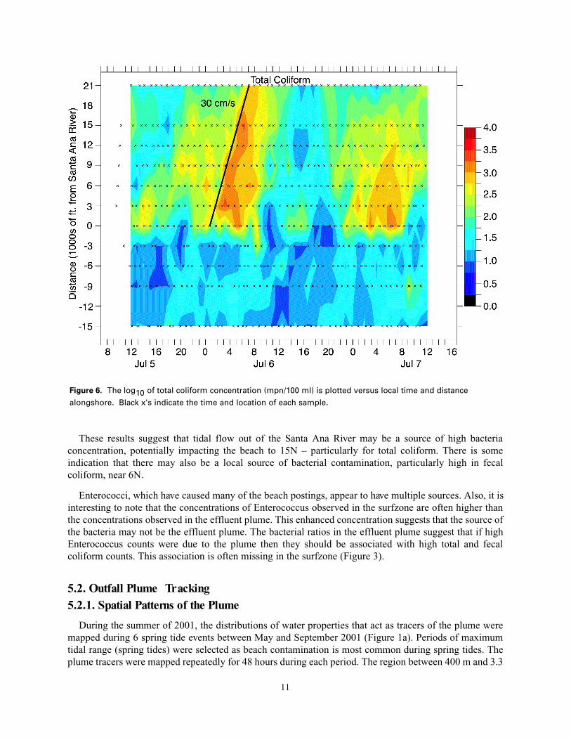
Even though total coliform has a day-night cycle, it shows a stronger relationship to the semidiurnaltidal cycle. The highest values are found preferentially near low tide at station 0 (next to the mouth of theSanta Ana River) and nearby stations to the north of it. Data also suggest that there is upcoast(northwestward propagation) from station 0, with a speed of about 30 cm/s (0.7 mph) (Figure 6).

These results suggest that total and fecal coliform levels are controlled principally by the phase of thetide. Enterococci seem to be controlled more by the day-night cycle. However, we can not definitivelyseparate the two effects because the hourly sampling programs were separated by about two weeks. Hence,night samples were always taken on the larger ebb tide. Also, without reliable information as to the die-offrate of the different bacterial indicators under the prevailing light, temperature, and salinity conditions, wecannot say how the temporal patterns are influenced by the bacterial life span.

10

Figure 5. The ratio of Enterococci concentrations to the AB411 single sample standard at stations 15S to 21N forthe 2nd intensive sampling period are plotted together with sampling times at station 0 (pink dots), Los Angelessea level (red line), and temperature 0.5m above bottom at HB01 (blue line). Only samples exceeding 104mpn/100ml are shown here. A local time reference is used.

These results suggest that tidal flow out of the Santa Ana River may be a source of high bacteriaconcentration, potentially impacting the beach to 15N – particularly for total coliform. There is someindication that there may also be a local source of bacterial contamination, particularly high in fecalcoliform, near 6N.

Enterococci, which have caused many of the beach postings, appear to have multiple sources. Also, it isinteresting to note that the concentrations of Enterococcus observed in the surfzone are often higher thanthe concentrations observed in the effluent plume. This enhanced concentration suggests that the source ofthe bacteria may not be the effluent plume. The bacterial ratios in the effluent plume suggest that if highEnterococcus counts were due to the plume then they should be associated with high total and fecalcoliform counts. This association is often missing in the surfzone (Figure 3).

5.2. Outfall Plume Tr acking

5.2.1. Spatial Patterns of the Plume

During the summer of 2001, the distributions of water properties that act as tracers of the plume weremapped during 6 spring tide events between May and September 2001 (Figure 1a). Periods of maximumtidal range (spring tides) were selected as beach contamination is most common during spring tides. Theplume tracers were mapped repeatedly for 48 hours during each period. The region between 400 m and 3.3

11

Figure 6. The log10 of total coliform concentration (mpn/100 ml) is plotted versus local time and distance

alongshore. Black x's indicate the time and location of each sample.

km (0.25 to 2 miles) offshore of the beach was mapped at 4-hour intervals with CTD profiles, resulting in12 realizations during each period. The region between 3.3 km (2 miles) and beyond the shelf break wasmapped with a towed undulating vehicle every 8 hours, which produced up to 6 three-dimensional mapsof the offshore region during each period.

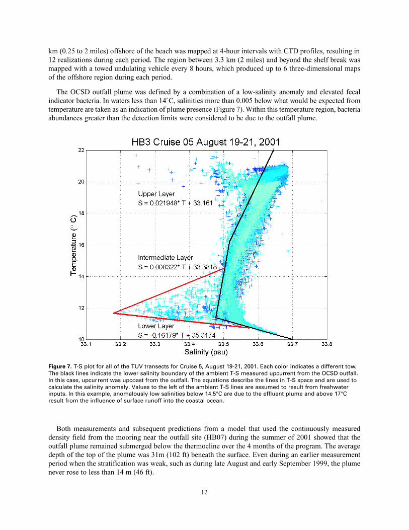
The OCSD outfall plume was defined by a combination of a low-salinity anomaly and elevated fecalindicator bacteria. In waters less than 14˚C, salinities more than 0.005 below what would be expected fromtemperature are taken as an indication of plume presence (Figure 7). Within this temperature region, bacteriaa bundances greater than the detection limits were considered to be due to the outfall plume.

Both measurements and subsequent predictions from a model that used the continuously measureddensity field from the mooring near the outfall site (HB07) during the summer of 2001 showed that theoutfall plume remained submerged below the thermocline over the 4 months of the program. The averagedepth of the top of the plume was 31m (102 ft) beneath the surface. Even during an earlier measurementperiod when the stratification was weak, such as during late August and early September 1999, the plumenever rose to less than 14 m (46 ft).

12

Figure 7. T-S plot for all of the TUV transects for Cruise 5, August 19-21, 2001. Each color indicates a different tow.The black lines indicate the lower salinity boundary of the ambient T-S measured upcurrent from the OCSD outfall.In this case, upcurrent was upcoast from the outfall. The equations describe the lines in T-S space and are used tocalculate the salinity anomaly. Values to the left of the ambient T-S lines are assumed to result from freshwaterinputs. In this example, anomalously low salinities below 14.5°C are due to the effluent plume and above 17°Cresult from the influence of surface runoff into the coastal ocean.

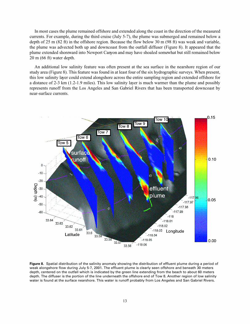
In most cases the plume remained offshore and extended along the coast in the direction of the measuredcurrents. For example, during the third cruise (July 5-7), the plume was submerged and remained below adepth of 25 m (82 ft) in the offshore region. Because the flow below 30 m (98 ft) was weak and variable,the plume was advected both up and downcoast from the outfall diffuser (Figure 8). It appeared that theplume extended shoreward into Newport Canyon and may have shoaled somewhat but still remained below20 m (66 ft) water depth.

An additional low salinity feature was often present at the sea surface in the nearshore region of ourstudy area (Figure 8). This feature was found in at least four of the six hydrographic surveys. When present,this low salinity layer could extend alongshore across the entire sampling region and extended offshore fora distance of 2-3 km (1.2-1.9 miles). This low salinity layer is much warmer than the plume and possiblyrepresents runoff from the Los Angeles and San Gabriel Rivers that has been transported downcoast bynear-surface currents.

13

Figure 8. Spatial distribution of the salinity anomaly showing the distribution of effluent plume during a period ofweak alongshore flow during July 5-7, 2001. The effluent plume is clearly seen offshore and beneath 30 metersdepth, centered on the outfall which is indicated by the green line extending from the beach to about 60 metersdepth. The diffuser is the portion of the line underneath the offshore end of Tow 8. Another region of low salinitywater is found at the surface nearshore. This water is runoff probably from Los Angeles and San Gabriel Rivers.

5.2.2. Bacteria Concentrations

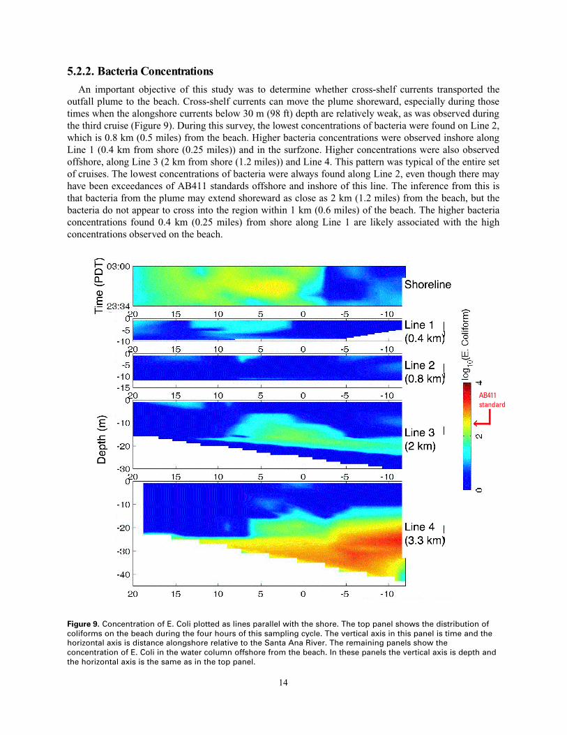
An important objective of this study was to determine whether cross-shelf currents transported theoutfall plume to the beach. Cross-shelf currents can move the plume shoreward, especially during thosetimes when the alongshore currents below 30 m (98 ft) depth are relatively weak, as was observed duringthe third cruise (Figure 9). During this survey, the lowest concentrations of bacteria were found on Line 2,which is 0.8 km (0.5 miles) from the beach. Higher bacteria concentrations were observed inshore alongLine 1 (0.4 km from shore (0.25 miles)) and in the surfzone. Higher concentrations were also observedoffshore, along Line 3 (2 km from shore (1.2 miles)) and Line 4. This pattern was typical of the entire setof cruises. The lowest concentrations of bacteria were always found along Line 2, even though there mayhave been exceedances of AB411 standards offshore and inshore of this line. The inference from this isthat bacteria from the plume may extend shoreward as close as 2 km (1.2 miles) from the beach, but thebacteria do not appear to cross into the region within 1 km (0.6 miles) of the beach. The higher bacteriaconcentrations found 0.4 km (0.25 miles) from shore along Line 1 are likely associated with the highconcentrations observed on the beach.

14

Figure 9. Concentration of E. Coli plotted as lines parallel with the shore. The top panel shows the distribution ofcoliforms on the beach during the four hours of this sampling cycle. The vertical axis in this panel is time and thehorizontal axis is distance alongshore relative to the Santa Ana River. The remaining panels show theconcentration of E. Coli in the water column offshore from the beach. In these panels the vertical axis is depth andthe horizontal axis is the same as in the top panel.

A B 4 1 1standard

Fecal indicator bacteria in the submerged effluent plume were well correlated with each other. The ratioof total coliform: fecal coliform: Enterococcus is typically about 25:5:1 in the main body of the plume.This ratio is relatively constant with distance away from the outfall discharge. This suggests that die-offrates for the 3 bacterial species in the plume may be relatively uniform in this environment. In earlierplume tracking surveys (MEC, 2001), high bacteria concentrations were observed at least 12.5 km (7.8miles) downcoast from the outfall. Transit times from the outfall were estimated to be on the order of 2days. Both these results suggest that the die-off rates of the bacteria may be low in the center of the plume,where the waters are dark and cold.

The ratios among the 3 fecal indicator bacteria become more va r i a ble at lower bacterial concentrations.Enterococcus appears to decrease more rapidly compared to total coliform bacteria when the Enterococcusconcentrations falls below 100 MPN/100 ml and total coliform bacteria fall below 1000 MPN/100 ml.Whether this is real or an artifact of increased variability at lower concentrations is uncertai n .

5.3. Coastal Tr ansport Processes

5.3.1. Subtidal Tr ansport

When currents associated with the tides and sea breeze are removed from the records, the remainingflows are substantial and play the major role in the longer term dispersal of the outfall plume. These lowfrequency or subtidal flows have patterns that are caused by circulation processes over the larger scalecoastal region of the Southern California Bight. In the summer, there is a substantial down-coast (towardsSan Diego) mean current over the San Pedro shelf that has a maximum near the surface on the outer shelf.This down-coast flow decreases in magnitude with depth and toward shore. It is generally unrelated to localwinds over the shelf. However, there is some indication that these subtidal fluctuations in along-coast floware related to wind forcing off central Baja California (via coastal trapped wave propagation). Figure 10shows the mean current vectors for the period of summer 2001. Surface mean currents of 10 to 12 cm/s(0.2 mph) on the outer shelf can transport material down-coast a distance of 10 km (6 miles) in one day.

At depths below about 70 m (230 ft) over the San Pedro continental slope, seaward of the outfall, theflow is predominantly up-coast (towards Palos Verdes) and constitutes an undercurrent. This undercurrentoccasionally rises to shallower depths for a few days and floods the outer shelf with up-coast currents.Figure 10 shows that at depths below about 30 m (98 ft) on the outer shelf, the mean flows are directedweakly up-coast.

Imposed on this mean flow pattern are fluctuations with periods of 7 to 20 days that have a magnitudesimilar to the mean flow. T h ey are largest at the surface and on the outer shelf and decrease with depth andt owards shore. In the upper layers, the currents are parallel to the general trend of the coastline, but in the lowe rl ayers the currents follow the trend of the depth contours (isobaths). Shorter period (7 day) fluctuationsdominate in the near shore (depths < 15 m (49ft)). Maximum currents can exceed 60 and 30 cm/s (1.3-0.7mph) on the outer and inner shelf, respective ly. Given the long periods of the fluctuations, the low frequencys u r face currents can be set in the same along-coast direction for periods on the order of we e k s .

The fluctuations across the shelf and with depth are generally all in the same direction at any given time.However, in the near shore, alongshelf current fluctuations are found to be closely related to the alongshorewinds and somewhat disconnected from currents on the middle and outer shelf. This means that flows inthe near shore may be in the opposite direction to flows over the middle and outer shelf. This provides acurrent regime in which plume material could be transported down coast towards the Newport Canyon byflows over the outer shelf, and then be transported up coast by the reversed nearshore currents.

15

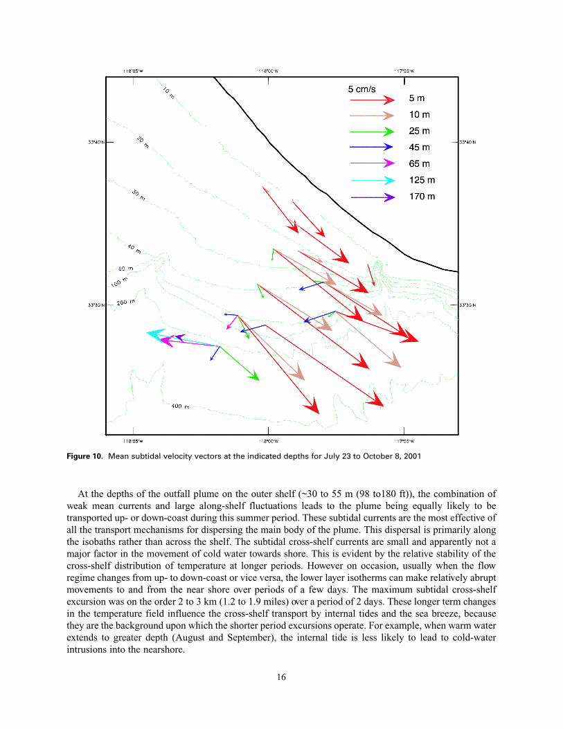
At the depths of the outfall plume on the outer shelf (~30 to 55 m (98 to180 ft)), the combination ofweak mean currents and large along-shelf fluctuations leads to the plume being equally likely to betransported up- or down-coast during this summer period. These subtidal currents are the most effective ofall the transport mechanisms for dispersing the main body of the plume. This dispersal is primarily alongthe isobaths rather than across the shelf. The subtidal cross-shelf currents are small and apparently not amajor factor in the movement of cold water towards shore. This is evident by the relative stability of thecross-shelf distribution of temperature at longer periods. However on occasion, usually when the flowregime changes from up- to down-coast or vice versa, the lower layer isotherms can make relatively abruptmovements to and from the near shore over periods of a few days. The maximum subtidal cross-shelfexcursion was on the order 2 to 3 km (1.2 to 1.9 miles) over a period of 2 days. These longer term changesin the temperature field influence the cross-shelf transport by internal tides and the sea breeze, becausethey are the background upon which the shorter period excursions operate. For example, when warm waterextends to greater depth (August and September), the internal tide is less likely to lead to cold-waterintrusions into the nearshore.

16

Figure 10. Mean subtidal velocity vectors at the indicated depths for July 23 to October 8, 2001

5.3.2. Diurnal and Semidiurnal Tr ansport

5.3.2.1. Seabreeze and Diurnal Currents

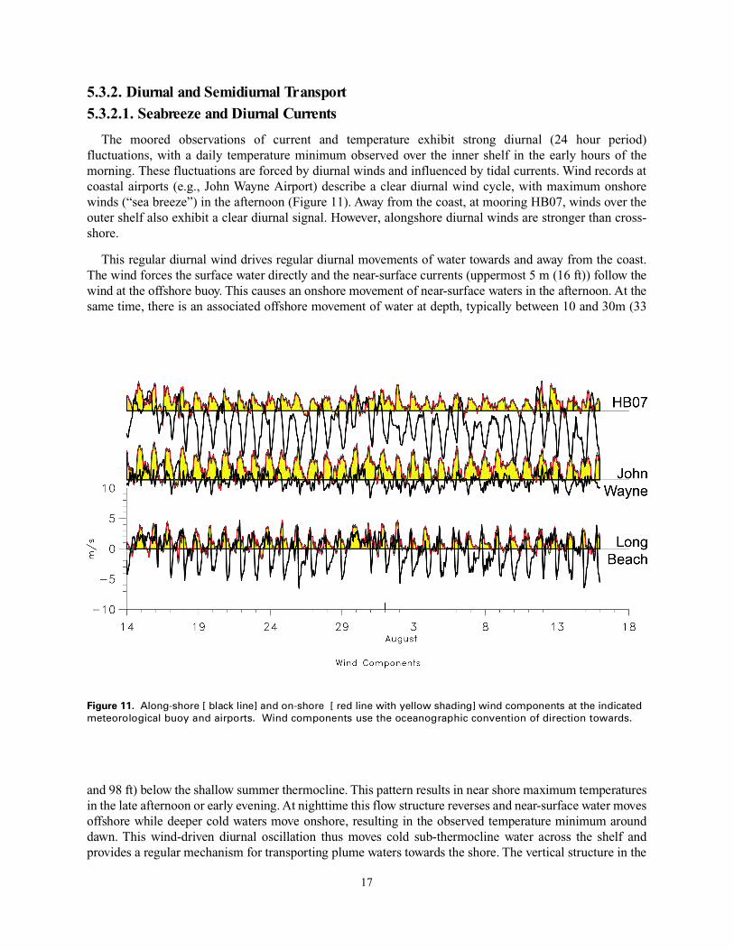
The moored observations of current and temperature exhibit strong diurnal (24 hour period)fluctuations, with a daily temperature minimum observed over the inner shelf in the early hours of themorning. These fluctuations are forced by diurnal winds and influenced by tidal currents. Wind records atcoastal airports (e.g., John Wayne Airport) describe a clear diurnal wind cycle, with maximum onshorewinds (“sea breeze”) in the afternoon (Figure 11). Away from the coast, at mooring HB07, winds over theouter shelf also exhibit a clear diurnal signal. However, alongshore diurnal winds are stronger than cross-shore.

This regular diurnal wind drives regular diurnal movements of water towards and away from the coast.The wind forces the surface water directly and the near- s u r face currents (uppermost 5 m (16 ft)) follow thewind at the offshore bu oy. This causes an onshore movement of near- s u r face waters in the afternoon. At thesame time, there is an associated offshore movement of water at depth, typically between 10 and 30m (33

and 98 ft) below the shallow summer thermocline. This pattern results in near shore maximum temperaturesin the late afternoon or early evening. At nighttime this flow structure reverses and near- s u r face water move so ffshore while deeper cold waters move onshore, resulting in the observed temperature minimum aroundd awn. This wind-driven diurnal oscillation thus moves cold sub-thermocline water across the shelf andp r ovides a regular mechanism for transporting plume waters towards the shore. The ve rtical structure in the

17

F i g u re 11. A l o n g - s h o re [ black line] and on-shore [ red line with yellow shading] wind components at the indicatedm e t e o rological buoy and airports. Wind components use the oceanographic convention of direction toward s .

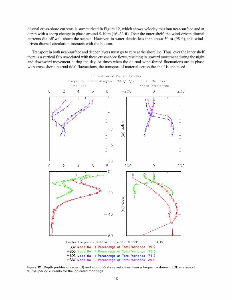
d i u rnal cross-shore currents is summarized in Figure 12, which shows velocity maxima near- s u r face and atdepth with a sharp change in phase around 5-10 m (16 -33 ft). Over the outer shelf, the wind-driven diurn a lc u rrents die off well above the seabed. Howeve r, in water depths less than about 30 m (98 ft), this wind-d r iven diurnal circulation interacts with the bottom.

Tr a n s p o rt in both near- s u r face and deeper layers must go to zero at the shoreline. Thus, over the inner shelfthere is a ve rtical flux associated with these cross-shore flows, resulting in upward movement during the nightand dow n ward movement during the day. At times when the diurnal wind-forced fluctuations are in phasewith cross-shore internal tidal fluctuations, the transport of material across the shelf is enhanced.

18

Figure 12. Depth profiles of cross (U) and along (V) shore velocities from a frequency domain EOF analysis ofdiurnal period currents for the indicated moorings.

5.3.2.2. Semidiurnal Currents

The semidiurnal (12 hour period) tidal currents are composed of two distinct current fields. Thei n d ividual barotropic tidal constituents have a constant amplitude with time and a uniform velocity withdepth. Within a tidal band, such as the semidiurnal band, the separate semidiurnal tidal constituents M2 andS2 can reinforce or partially nullify each other. This causes the 14.8-day spring/neap cycle that is mostclearly seen in sea level records. The individual constituents of the baroclinic, or internal, tidal currentsh ave amplitudes that va ry over periods of days to a week or two. T h ey also have a pronounced shear withdepth. Usually, internal tidal currents near the surface and near the bed flow in opposite directions.

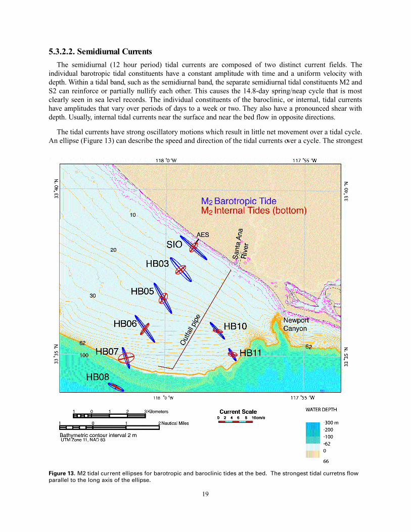
The tidal currents have strong oscillatory motions which result in little net movement over a tidal cycle.An ellipse (Figure 13) can describe the speed and direction of the tidal currents over a cycle. The strongest

19

Figure 13. M2 tidal current ellipses for barotropic and baroclinic tides at the bed. The strongest tidal curretns flowparallel to the long axis of the ellipse.

currents flow parallel to the long axis of the ellipse. The length of the major axis represents the strength ofthe flow. For semidiurnal tides, the currents 3 hours later are weaker and flow parallel to the ellipse’s minoraxis. Six hours later, the currents again flow parallel to the long axis of the ellipse, but in the oppositedirection of the previous flow. Twelve hours later, the currents return to their original direction and speed.

On the outer shelf, barotropic tidal current ellipses are aligned halfway between the along and cross-shelfdirections (Figure 13). Internal tidal current ellipses are aligned approx i m a t e ly perpendicular to the coast.C l e a r ly, each average cross shore tidal current constituent, with speeds around 2-3 cm/s (0.7-1.ft/s), will notm ove plume water or suspended effluent material from where it is discharged at the shelf break to thenearshore. Water is transported onshore by an average flood tide a distance of about 0.4 km, an insignifi c a n tp o rtion of the distance from the outfall to the shore. If all tidal constituents reinforce each other, tidal curr e n t scan flow across the shelf with combined speeds of 5-10 cm/s. Thus water is transported onshore by an ave r a g eflood tide 0.9 to 1.5 km (0.6 to 0.9 mile), less than 1/5 of the distance from the outfall to the shore. When thetidal currents ebb, the average tidal current will carry the water about the same distance offshore, causinglittle net movement of suspended material. As one nears the coast, cross-shelf transport by tidal currents iseven more limited because barotropic tidal currents flow parallel to shore (Figure 13); only internal tidalc u rrents can transport water and suspended material toward the coast.

However, the semidiurnal internal tidal currents do not have constant amplitude over the summermonths. They can be larger or smaller than their average amplitude for periods of days to weeks. It isinteresting to note that the times when internal tides are large are not tied to the spring/neap cycle. If dailywind or other diurnal forcing reinforces one of the two semidiurnal current pulses, the internal tides mayalso have a pronounced mixed tidal signal. That is, every other tidal current pulse can be noticeably largerthan the preceding pulse. During the summer of 2001, large internal tidal currents appeared at thebeginning and end of July and in late August. Cross-shore current speeds near the bed at the end of Julywere larger than 10 cm/s.

5.3.2.3. Cross-Shor e Tr ansport Events in Coastal Ocean Currents

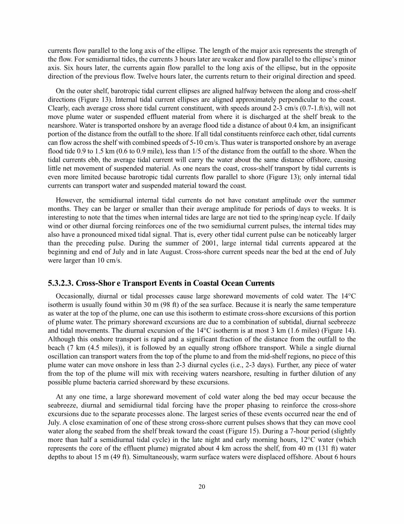
O c c a s i o n a l ly, diurnal or tidal processes cause large shoreward movements of cold wa t e r. The 14°Ci s o t h e rm is usually found within 30 m (98 ft) of the sea surface. Because it is nearly the same temperatureas water at the top of the plume, one can use this isotherm to estimate cross-shore excursions of this port i o nof plume wa t e r. The primary shoreward excursions are due to a combination of subtidal, diurnal seebreezeand tidal movements. The diurnal excursion of the 14°C isotherm is at most 3 km (1.6 miles) (Figure 14).Although this onshore transport is rapid and a significant fraction of the distance from the outfall to thebeach (7 km (4.5 miles)), it is followed by an equally strong offshore transport. While a single diurn a loscillation can transport waters from the top of the plume to and from the mid-shelf regions, no piece of thisplume water can move onshore in less than 2-3 diurnal cycles (i.e., 2-3 days). Furt h e r, any piece of wa t e rfrom the top of the plume will mix with receiving waters nearshore, resulting in further dilution of anyp o s s i ble plume bacteria carried shoreward by these ex c u r s i o n s .

At any one time, a large shoreward movement of cold water along the bed may occur because theseabreeze, diurnal and semidiurnal tidal forcing have the proper phasing to reinforce the cross-shoreexcursions due to the separate processes alone. The largest series of these events occurred near the end ofJuly. A close examination of one of these strong cross-shore current pulses shows that they can move coolwater along the seabed from the shelf break toward the coast (Figure 15). During a 7-hour period (slightlymore than half a semidiurnal tidal cycle) in the late night and early morning hours, 12°C water ( wh i c hrepresents the core of the effluent plume) migrated about 4 km across the shelf, from 40 m (131 ft) waterdepths to about 15 m (49 ft). Simultaneously, warm surface waters were displaced offshore. About 6 hours

20

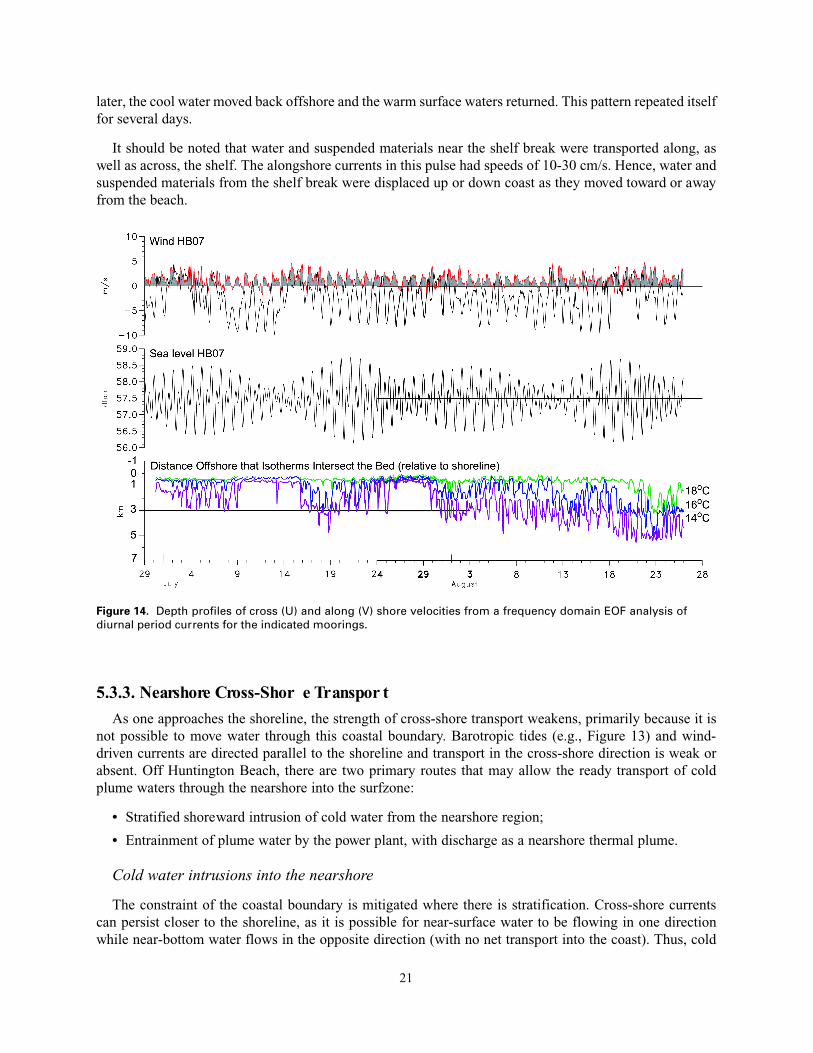
later, the cool water moved back offshore and the warm surface waters returned. This pattern repeated itselffor several days.

It should be noted that water and suspended materials near the shelf break were transported along, aswell as across, the shelf. The alongshore currents in this pulse had speeds of 10-30 cm/s. Hence, water andsuspended materials from the shelf break were displaced up or down coast as they moved toward or awayfrom the beach.

5.3.3. Nearshore Cross-Shor e Tr anspor t

As one approaches the shoreline, the strength of cross-shore transport weakens, primarily because it isnot possible to move water through this coastal boundary. Barotropic tides (e.g., Figure 13) and wind-driven currents are directed parallel to the shoreline and transport in the cross-shore direction is weak orabsent. Off Huntington Beach, there are two primary routes that may allow the ready transport of coldplume waters through the nearshore into the surfzone:

• Stratified shoreward intrusion of cold water from the nearshore region;

• Entrainment of plume water by the power plant, with discharge as a nearshore thermal plume.

Cold water intrusions into the nearshore

The constraint of the coastal boundary is mitigated where there is stratification. Cross-shore currentscan persist closer to the shoreline, as it is possible for near-surface water to be flowing in one directionwhile near-bottom water flows in the opposite direction (with no net transport into the coast). Thus, cold

21

Figure 14. Depth profiles of cross (U) and along (V) shore velocities from a frequency domain EOF analysis ofdiurnal period currents for the indicated moorings.

22

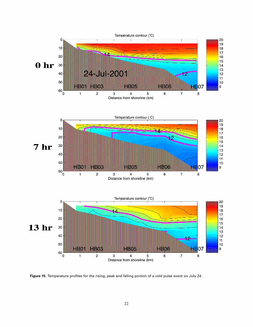
Figure 15. Temperature profiles for the rising, peak and falling portion of a cold pulse event on July 24.

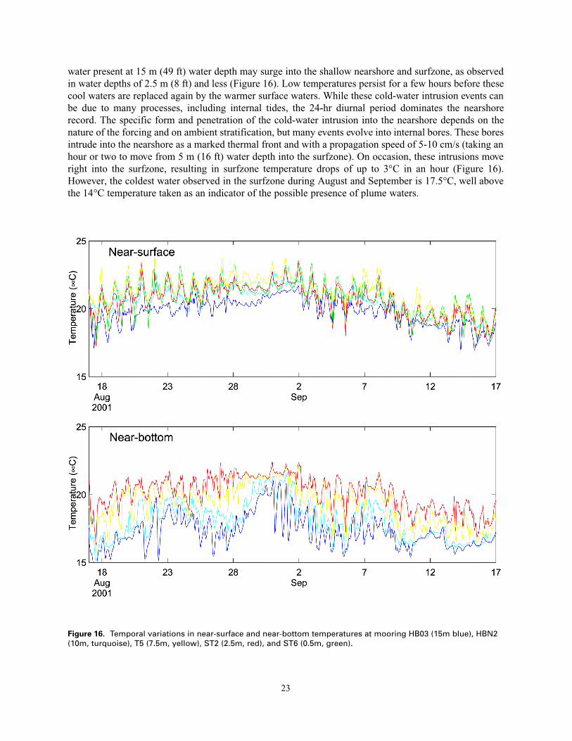
water present at 15 m (49 ft) water depth may surge into the shallow nearshore and surfzone, as observedin water depths of 2.5 m (8 ft) and less (Figure 16). Low temperatures persist for a few hours before thesecool waters are replaced again by the warmer surface waters. While these cold-water intrusion events canbe due to many processes, including internal tides, the 24-hr diurnal period dominates the nearshorerecord. The specific form and penetration of the cold-water intrusion into the nearshore depends on thenature of the forcing and on ambient stratification, but many events evolve into internal bores. These boresintrude into the nearshore as a marked thermal front and with a propagation speed of 5-10 cm/s (taking anhour or two to move from 5 m (16 ft) water depth into the surfzone). On occasion, these intrusions moveright into the surfzone, resulting in surfzone temperature drops of up to 3°C in an hour (Figure 16).However, the coldest water observed in the surfzone during August and September is 17.5°C, well abovethe 14°C temperature taken as an indicator of the possible presence of plume waters.

23

Figure 16. Temporal variations in near-surface and near-bottom temperatures at mooring HB03 (15m blue), HBN2(10m, turquoise), T5 (7.5m, yellow), ST2 (2.5m, red), and ST6 (0.5m, green).

AES power plant

Due to its location, the AES power plant has been suspected of directly contributing to the contaminationof the beach between 3N and 9N. The power plant pumps in cooling water at 8.4 m (27 ft) water depth andthen discharges heated water at 6.5 m (21 ft) water depth. Three potential roles have been identified.

a. Thermal stratification could enhance cold-water intrusions into the nearshore: During the period ofplant operation in late summer (including both reduced cooling water flows in July-August andstronger flows in September-October), there is no evidence of a difference in the currents at 10 moffshore of the power plant and at a comparable 10 m location 2 km (1.2 miles) further upcoast.Further, the calculated heat load and observed thermal plume stratification are not sufficient tosignificantly alter the stratification and cold-water intrusions dynamics.

b. Pumping of cooling water through the power plant enhances shoreward transport of bottom water from8.4 m (27 ft) water depth: As is evident in Figure 16, colder water reaches the depth of the power planti n t a ke and discharge (see thermistor at 7.5 m (25 ft) water depth) more often than it intrudes into thesurfzone (see thermistors at 2.5 m (8 ft) and 0.5 m (1.6 ft) water depths). Once entrained by the intakeor discharge jet, this potentially contaminated cold water forms part of the surface thermal plume thatis observed nearshore and can be expected to move into the surfzone through bu oyant spreading orunder the action of afternoon winds and other ambient processes. Surfzone temperature observa t i o n ss h owed limited effects of the thermal plume, indicating that these waters had been well mixed beforeimpacting the beach (dilutions of at least 10-fold). While the power plant was not operating in earlys u m m e r, the observation of beach contamination events during that time period indicates that the powe rplant does not play an essential role in beach contamination.

c. The power plant may act as a source or conduit for bacteria moving from land to ocean. The role ofthe power plant in beach contamination is presently the subject of a California Energy Commissionstudy, aiming to assess this question through extensive sampling of bacteria concentrations in theplant during 2002. The possible role of the plant in the transport of wastewater to the beach is beingassessed through concurrent sampling of intake water temperatures, salinity, ammonia and fecalbacteria concentrations.

5.3.4. Sediment Resuspension

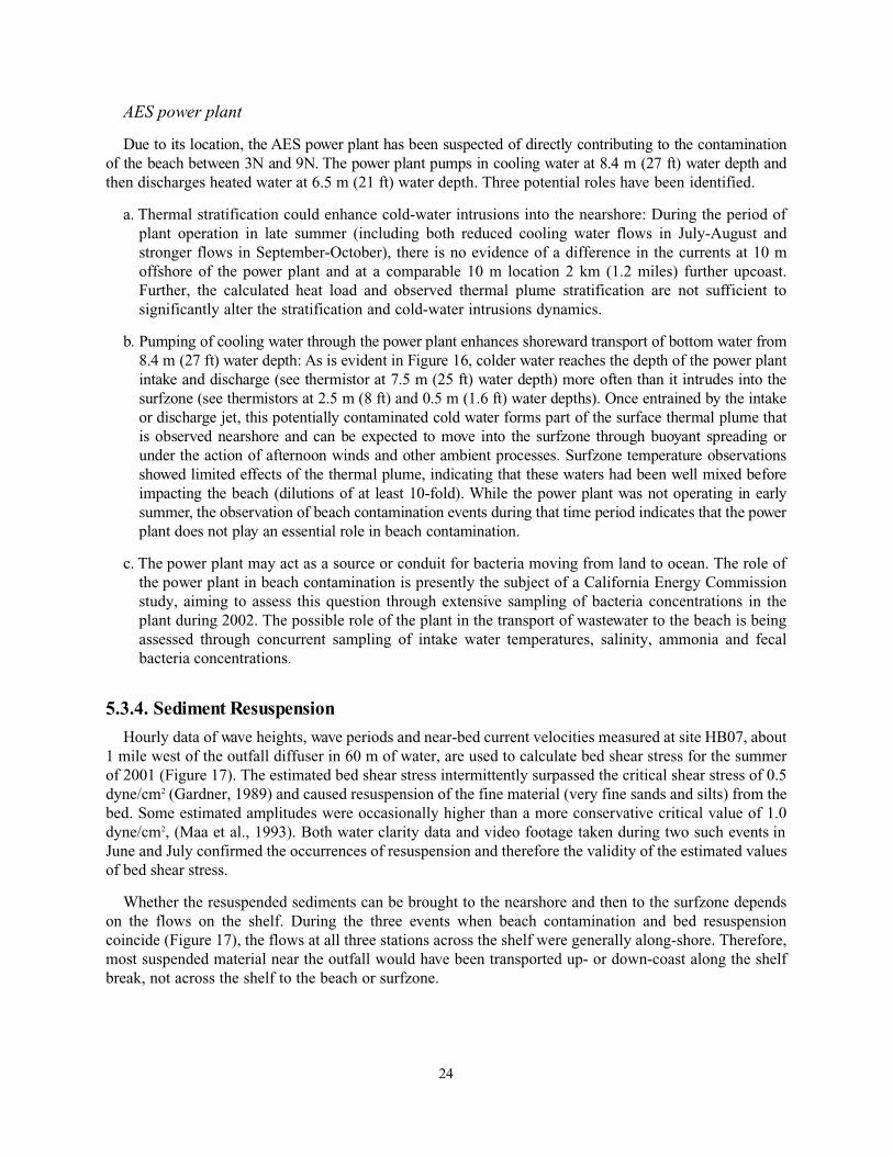
Hourly data of wave heights, wave periods and near-bed current velocities measured at site HB07, about1 mile west of the outfall diffuser in 60 m of water, are used to calculate bed shear stress for the summerof 2001 (Figure 17). The estimated bed shear stress intermittently surpassed the critical shear stress of 0.5dyne/cm2 (Gardner, 1989) and caused resuspension of the fine material (very fine sands and silts) from thebed. Some estimated amplitudes were occasionally higher than a more conservative critical value of 1.0dyne/cm2, (Maa et al., 1993). Both water clarity data and video footage taken during two such events inJune and July confirmed the occurrences of resuspension and therefore the validity of the estimated valuesof bed shear stress.

Whether the resuspended sediments can be brought to the nearshore and then to the surfzone dependson the flows on the shelf. During the three events when beach contamination and bed resuspensioncoincide (Figure 17), the flows at all three stations across the shelf were generally along-shore. Therefore,most suspended material near the outfall would have been transported up- or down-coast along the shelfbreak, not across the shelf to the beach or surfzone.

24

6. COASTAL TRANSPORT PROCESSES AND THEIR RELATIONSHIP TOSIGNIFICANT SURFZONE B ACTERIAL P ATTERNS

The temporal relationships between the three categories of surfzone bacterial exceedance events definedearlier (section 5.1.2) and the various coastal oceanographic processes were used to determine theprobability that significant levels of bacteria from the outfall were transported to the beach.

6.1. Subtidal Cross-Shelf Tr ansport, Newport Can yon

Occasionally, the along-isobath subtidal currents in the near shore region flow in the opposite directionto currents over the middle and outer shelf. This provides a current regime in which plume material couldbe transported downcoast towards the Newport Canyon and then transported up coast by the reversednearshore currents. Because this plume water is relatively close to shore, other coastal ocean processes maycarry this water to local beaches.

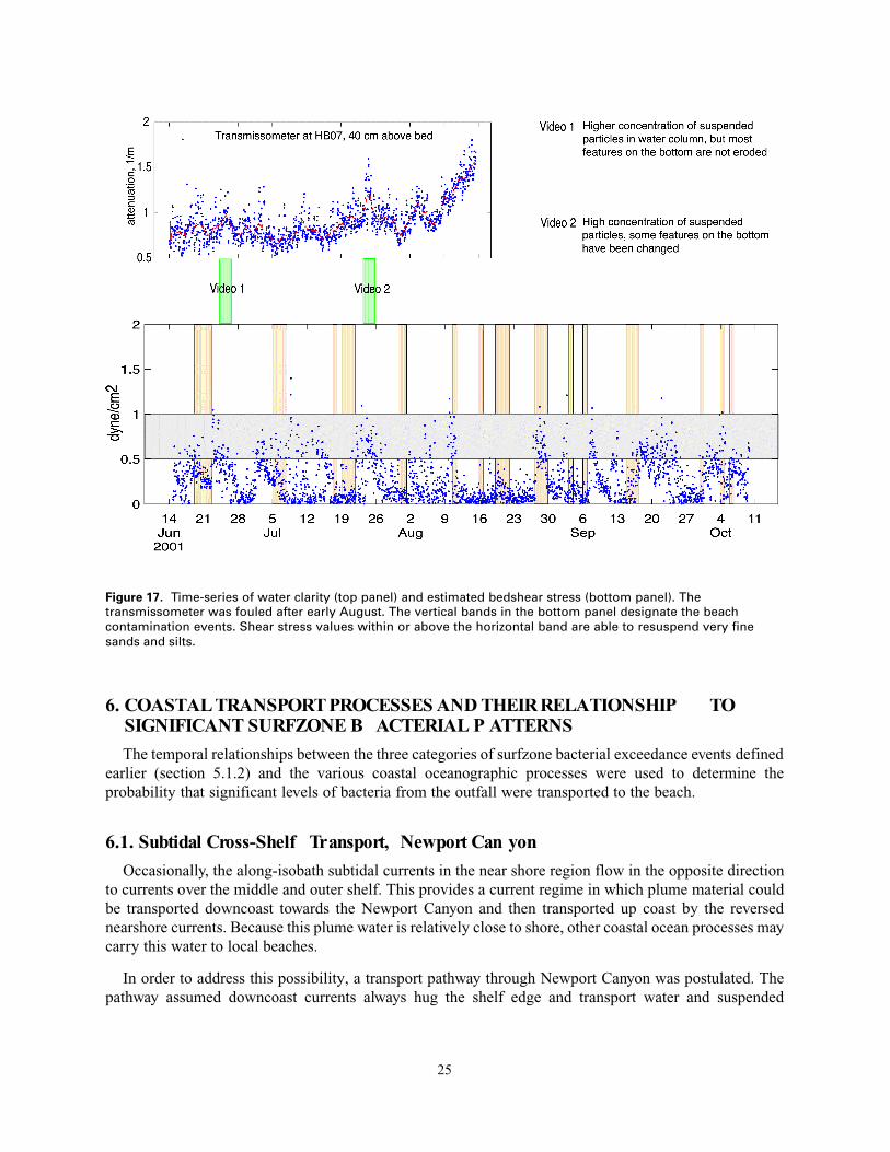
In order to address this possibility, a transport pathway through Newport Canyon was postulated. Thepathway assumed downcoast currents always hug the shelf edge and transport water and suspended

25

Figure 17. Time-series of water clarity (top panel) and estimated bedshear stress (bottom panel). Thetransmissometer was fouled after early August. The vertical bands in the bottom panel designate the beachcontamination events. Shear stress values within or above the horizontal band are able to resuspend very finesands and silts.

materials toward the canyon (Figure 18), if the downcoast flow is persistent, water from near the outfallcan reach the canyon. We hypothesized that canyon upwelling will then transport this subsurface plumewater onto the adjacent shelf. If upcoast flows exist at that time, this plume water will then be transportedto the nearshore water off Huntington Beach. The possibly contaminated water will continue to remain

26

Figure 18. Hypothetical transport of effluent plume through Newport Canyon and table of related events.

offshore of Huntington Beach as long as the transport pathway remains intact. Various nearshore, cross-shore transport processes could bring the bacteria to the beach. This is a very idealized pathway that favorstransport of plume material through Newport Canyon. It ignores the fact that the plume often exits the shelfin the downcoast direction and moves into much deeper water. It also ignores the possibility that canyonupwelling may not exist when the pathway is in existence.

We assessed the currents along the pathway and found that water from near the outfall could havereached Newport Canyon 7 times during the summer of 2001 (Figure 18). The nearshore upcoast flow waspersistent enough in 4 of these events that plume water could have been carried to Huntington Beach.During the postulated time windows when the plume water would have been offshore of HuntingtonBeach, only one surfzone measurement was above the AB411 standards. Broadening the window by oneday on each side yielded two more possible contamination days. However, these events, which occurred onthe first day of an expanded window, were at the end of an earlier 3 day beach contamination event. Henceit is unlikely they were associated with the Newport Canyon pathway.

The potential for transport through New p o rt Canyon did not commonly occur in the summer of 2001.The pathway was only open for 7-13% of the days in the study period for the actual and expanded window s ,r e s p e c t ive ly. The actual and expanded windows were associated with only 1 to 3 of the 42 days when eithera Type 1-3 contamination event occurred during the study period from June to October 2001.

6.2. Diurnal and Semidiurnal Tr ansport Pathways

As individual mechanisms, the diurnal wind-driven and barotropic tidal oscillations can move cold sub-thermocline water toward the shore, although the distance of the excursions is relatively small. Theexcursion of these motions separately is insufficient to move plume water into the nearshore in less thantwo days, unless assisted by some other transport mechanism. Furthermore, the portion of plume watermost likely to be transported by the diurnal seabreeze mechanisms is from the top of the plume, which hasmuch smaller bacterial concentrations than the core of the plume. Any piece of plume water transportedby these mechanisms will mix with the receiving water nearshore, resulting in further dilution of bacterialconcentrations.

H i s t o r i c a l ly, the beaches are most like ly to be contaminated by bacteria during spring tides. It is not like lythat this contamination is predominately caused by cross-shelf transport of the outfall plume by large intern a ltides. The strongest internal tides did not tend to occur during spring tides over the 4-month study period.

6.3. Coastal Ocean Event Tr ansport Pathw ays

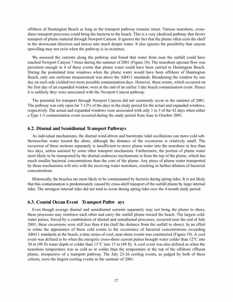
Even though average diurnal and semidiurnal currents separately may not bring the plume to shore,these processes may reinforce each other and carry the outfall plume toward the beach. The largest cold-water pulses, forced by a combination of diurnal and semidiurnal processes, occurred near the end of July2001; these excursions were still less than 4 km (half the distance from the outfall to shore). In an effortto relate the appearance of these cold events to the occurrence of bacterial concentrations exceedingAB411 standards at the beach, a time series of cool, near-shore events was constructed (Figure 19). A coolevent was defined to be when the energetic cross-shore current pulses brought water colder than 12°C into30 m (98 ft) water depth or colder than 13°C into 15 m (49 ft). A cool event was also defined as when thenearshore temperature was as cold as or colder than the temperature at the top of the offshore effluentplume, irrespective of a transport pathway. The July 23-26 cooling events, as judged by both of thesecriteria, were the largest cooling events in the summer of 2001.

27

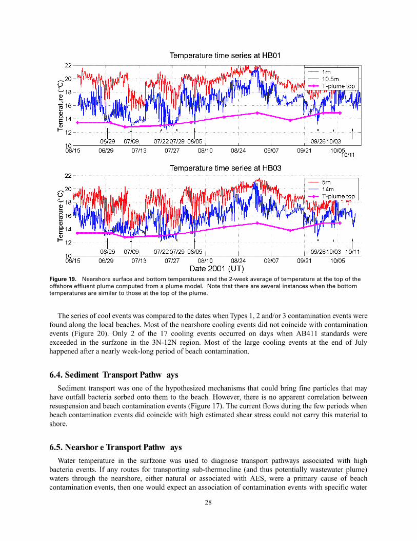
The series of cool events was compared to the dates when Types 1, 2 and/or 3 contamination events werefound along the local beaches. Most of the nearshore cooling events did not coincide with contaminationevents (Figure 20). Only 2 of the 17 cooling events occurred on days when AB411 standards wereexceeded in the surfzone in the 3N-12N region. Most of the large cooling events at the end of Julyhappened after a nearly week-long period of beach contamination.

6.4. Sediment Tr ansport Pathw ays

Sediment transport was one of the hypothesized mechanisms that could bring fine particles that mayhave outfall bacteria sorbed onto them to the beach. However, there is no apparent correlation betweenresuspension and beach contamination events (Figure 17). The current flows during the few periods whenbeach contamination events did coincide with high estimated shear stress could not carry this material toshore.

6.5. Nearshor e Tr ansport Pathw ays

Water temperature in the surfzone was used to diagnose transport pathways associated with highbacteria events. If any routes for transporting sub-thermocline (and thus potentially wastewater plume)waters through the nearshore, either natural or associated with AES, were a primary cause of beachcontamination events, then one would expect an association of contamination events with specific water

28

Figure 19. Nearshore surface and bottom temperatures and the 2-week average of temperature at the top of theoffshore effluent plume computed from a plume model. Note that there are several instances when the bottomtemperatures are similar to those at the top of the plume.

temperatures. If cold-water intrusions mediated contamination events, then one would expect high bacteriacounts to be associated with colder waters. Alternatively, if the power plant mediated contamination events,then one would expect high bacteria counts to be associated with warmer waters. None of theseassociations is apparent in the data. The results of the 2002 study of bacteria in the AES plant intake anddischarge are awaited to better resolve the viability of that transport pathway.

7. CONCLUSIONS

Although the study identifies several possible coastal ocean pathways by which diluted wastewater maybe transported to the beach, including internal tide, sea breeze, subtidal flow features and anthropogenicfeatures such as the AES cooling system, there were no direct observations of either the high bacteriaconcentrations seen in the OCSD plume at the shelf break reaching the shoreline in significant levels or ofan association between the existence of a coastal ocean process and beach contamination at or aboveAB411 levels. The only physical variables clearly identified as being related to surfzone contaminationwere phase of the lunar cycle, with high values of all three fecal indicator bacteria found preferentially atspring tides; time of day, with high values found at night – particularly for Enterococci; and phase of thetide, with high values found near low tide – particularly for total and fecal coliform bacteria. It isconcluded that the OCSD plume is not a major cause of beach contamination; no causal links could bedemonstrated. This conclusion is based on the absence of direct observation of links between bacteria inthe outfall plume and beach contamination, on analysis of spatial and temporal patterns of shorelinecontamination and coastal ocean processes, and on the observation of higher levels of contamination at thebeach than in the plume.

29

Figure 20. Days on which bacterial events occur (vertical bars: blue=type 1, magenta=type 2, red= types 1 and 2,gold=type 3) are shown together with cruise days (black bars); and occurrence of cold water nearshore (red= 12deg C inshore of 30m, blue =HB01 temperature < maximum plume temperature, green=both). Black dots in row 3indicate whether bacterial samples were taken that day. The day's higher high water as measured at Los Angelesis shown at the bottom.

8. REFERENCES

Gardner, W.D., 1989. Periodic resuspension in Baltimore Canyon by focusing of internal waves. JGR,94, 18185-18194

Grant, S., C. Webb, B. Sanders, A. Boehm, J. Kim, J. Redman, A. Chu, R. Mrse, S. Jiang, N.Gardiner, and A. Brown, 2000. Huntington Beach Water Quality Investigation Phase II: AnAnalysis of Ocean, Surf Zone, Watershed, Sediment and Groundwater Data Collected from June1998 through September 2000. Final Report.

Orange County Sanitation District, 1999. Huntington Beach Closure Report, Phase I final report.

Maa, J.P.-Y., L.D. Wright, C.-H. Lee, and T.W. Shannon, 1993. VIMS sea carousel: a field instrumentfor studying sediment transport. Marine Geology, 115, 271-287.

MEC (MEC Analytical Systems, Inc), 2000. Huntington Beach Closure: Relationships Between HighCounts of Bacteria on Huntington Beaches and Potential Sources. Final Report to OrangeCounty Sanitation District. January 2000. 13 pages plus tables and figures.

MEC (MEC Analytical Systems, Inc), 2001. Strategic Process Study, Plume Tracking. June 1999 toSeptemter 2000. Final Report, Volume I – Executive Summary.

SAIC and MEC, 1991. Proposed Elimination of Selected Water Quality Parameters, Total SuspendedSolids and Oil and Grease, and Reduction in Sampling Effort for Other Parameters From theOrange County Offshore Water Quality Monitoring Program. Final Report to Orange CountySanitation District. 12 pages plus appendices.

Acknowledgement

The authors would like to thank Jon Warrick for reviewing the report, and Lori Hibbeler for creating the HTML file.The on-line version of this report is at: http://geopubs.wr.usgs.gov/open-file/of03-62/

30