HUMAN CAPITAL INVESTMENTS IN EDUCATION AND HOME STABILITY: Exploring Education, Homeownership and Poverty

Jeffrey L. Jordan

Department of Agricultural and Applied Economics University of Georgia

Bulent Anil

Department of Economics University of Minnesota-Duluth

Velma Herbert and Swarn Chatterjee

Department of Housing and Consumer Economics University of Georgia

Paper presented at the Agricultural and Applied Economics Association Annual Meeting, Milwaukee, WS

In the best of times, investments in human capital in the form of spending on

education are successful when students arrive at school from stable homes. Yet a recent

report released by First Focus (Lovell and Isaacs, 2008), reveals that the home stability

of an estimated two million children is being affected by the sub-prime mortgage crisis as

their families face foreclosures. In addition, the report shows that these children are more

likely to experience excessive mobility and, as a result, are only half as likely to be

proficient in reading as their peers. Moreover, children forced from their homes

experience behavioral problems such as increases in violence. They are also much more

likely to be held back and eventually drop out of school.

This study offers an innovative way of capturing the benefits of homeownership

on children’s educational outcomes The paper draws on the results of earlier research

(Castillo, Ferraro, Jordan and Petrie) that looked at children’s time preferences as an

important component of educational outcomes by using economic experiments to

measure how children view the future. In particular, the study investigated the

relationships between time preferences and child demographics using a discount rate

2

experiment with middle school students in a Georgia school district. Time preferences

provide a measure for child patience---the less patient the student is with respect to

forgoing immediate benefits for larger benefits in the future, the more likely he or she is

to refrain from investing in school.

How these time preferences are formed remains unresolved ---what are the factors

that might cause impatient or irrational choices? Thus, this paper tests a hypothesis that

students who face housing uncertainties through mortgage foreclosures and eviction

learn impatient behavior and are therefore at greater risk of dropping out of school,

impeding human capital formation and community development..

To address this particular question we incorporate the results of a parent survey

which covers family housing situation --whether homeowner or renter, their demographic

characteristics (i.e., income, education, debt load, assets, net worth, gender, race, age,

marital status, number of children, tenure at work) and behavioral characteristics (risk

tolerance, confidence). The survey was administered to the parents of the eighth grade

students for which experiment data exists

The setting for this project is a county in Georgia, located on the southern end of

the Atlanta MSA. Although part of the vibrant metropolitan area of Atlanta,

demographic data on the county resembles less the exponential growth of the Atlanta area

and more the persistently poor counties of South Georgia. In 2000, per capita income was

$4,957 less than the State’s average and unemployment was 6.8%, or 24% higher than

the average. Thirty-two percent of persons over 25 have not completed high school in

2000 — over 50 percent higher than for all of Georgia. And, less than half (46.8%) of the

class of 2001 ninth graders graduated (this rate is 71.1% in Georgia), and the rate among

black males was even lower.

3

In terms of housing, this county is classified as on the Georgia’s “housing

stressed’ counties by the UGA Housing and Demographics Research Center (Tinsley,

2005). Further, city that is the county seat has chosen as a key initiative in the coming

years the issue of community housing and neighborhood revitalization. The elimination

of substandard housing and the reduction in the high home renter rate are city priorities.

The poorer neighborhoods of the nation face the major issues of poverty and lack of

homeownership, that affect their financial well being as well as the formation of their

social and human capital. Even though these issues of homeownership and poverty

alleviation have been well documented in the past (Gyourko & Linneman, 1997; Inc,

2003; Marcuse, 1989), little has been done to explore ways that can alleviate poverty

through sustainable homeownership in a neighborhood, without the displacement of its

existing inhabitants. While lack of homeownership and poverty alleviation are important

issues facing the nation as well as the state of Georgia, nowhere is it more prominent than

in this city. In the city and its surrounding areas a vast majority of households rent out

apartments. A significant portion of these renters pay out as much as 30% or more of

their monthly income for rent.

This paper will report on the results of a survey instrument that incorporates a

study of the respondents’ housing preferences --whether homeowner or renter, their

demographic characteristics (i.e., income, education, debt load, assets, net worth, gender,

race, age, marital status, number of children, tenure at work) and behavioral

characteristics (risk tolerance, confidence). The survey will be administered to the parents

of the eighth grade students for which experiment data exists.

4

2. Background Information

Much relevant recent literature has focused on conditions under which children

are raised and the potential consequences of these contextual factors for a variety of

outcomes in later life.1 Of particular importance for this study is emerging research that

examines the effects of the homeownership status of a family during child-rearing

periods. Although there is a considerable literature on the private and social benefits of

homeownership for such things as community participation, life satisfaction, home

maintenance, and accumulation of wealth (McCarthy, Van Zandt, and Rohe 2001; Rohe,

McCarthy, and Van Zandt 2000; Rossi and Weber 1996), only a few studies have

attempted to link any of these effects to later outcomes for children. The work of Green

and White (1997); Boehm and Schlottman (1999); Aaronson (2000); Boyle (2002);

Harkness and Newman (2002, 2003); Haurin, Parcel, and Haurin (2002a, 2002b); Haurin,

Dietz, and Weinberg (2003); and Kauppinen (2004) suggests that homeownership status

matters for children, although it is usually not clear whether the effect is an independent

one or is commingled with residential stability or neighborhood conditions, or both.

In particular, Green and White (1997) find a strong statistical correlation between

homeownership and the likelihood of dropping out of school or becoming pregnant. Yet a

reasonable interpretation of their result is that of omitted variable bias. Clearly,

homeowners are different from renters along a variety of dimensions. As a result, those

factors that are latent in their work, such as parental skills, interest in the educational

process, wealth, and family stability, potentially bias upward any homeownership effect.

While the authors claim that their results are robust to parametric self-selection

1Following studies offer comprehensive reviews of such literature: Earls and Carlson 2001; Ellen and

Turner 2003; Galster 2005; Leventhal and Brooks-Gunn 2000; Robert 1999; Sampson, Morenoff, and Gannon-Rowley 2002)

5

corrections, these techniques require assumptions about the selection equation that are

difficult to defend. However, beyond pure selection, there are several mechanisms that

suggest that this could be a causal relationship. Most plausibly, homeowners have a large

financial stake in their community and therefore may invest more in neighborhood and

school capital.

In addition, DiPasquale and Glaeser (1998) have modeled the different incentives

faced by owners and renters. Their key insight is that landlord’s recoup any community-

specific investment that is made by renters, while homeowners are able to internalize the

future returns to these investments because they accrue as increases in the value of their

home. Therefore, homeowners have a much stronger incentive to participate in the

growth of neighborhood capital. In fact, DiPasquale and Glaeser find that

homeownership has a causal effect on community investment. As investment in a

community grows, it is possible that educational outcomes will improve, perhaps

providing the missing link in the neighborhood effects literature. On the other hand, time

and money committed to neighborhood and housing investment might be offset by

reduced input into family-specific investments that have a more direct payoff to

children’s outcomes. For example, Currie and Yelowitz (2000) argue that public housing

has a positive effect on school retention because subsidized housing allows money to be

directed to other family needs.

An alternative but related mechanism works through family residential stability.

Several recent papers, including Hanushek, Kain and Rivkin (1999), Astone and

McLanahan (1991), and Haveman, Wolfe, and Spaulding (1991) explore the impact of

family or school mobility on student achievement. They argue that residential mobility

6

might be causal if it leads to a loss of social capital in the form of less information and

attachment to the school system, teachers, and peers.

The most convincing evidence is presented in Hanushek, Kain, and Rivkin, who,

using individual fixed effect models, find that residential or school moving has a

significant negative impact on student achievement, particularly for minorities, low

income families and students in schools with high turnover. Thus the homeownership

effect may be the result of additional family and school stability offered to students who

do not have to switch schools or peer groups. Moreover, Aaronson (2000) revisits this

issue and finds that parental homeownership in low-income neighborhood has a positive

impact on high school graduation. But he cautions that some of the positive effects might

rise due to the greater neighborhood stability (less residential movements) and not

necessarily to homeownership alone.

All of the above mentioned studies examine the direct effect of homeownership

on child outcomes. We approach this issue from a different perspective. It is well known

that children deal with inter-temporal problems, such as investment in education, in

different ways depending on their time preferences. Thus, we propose that if time

preferences or the perceived benefits of patience are formed in early childhood the home

stability might be a contributing factor to the formation of those. Becker and Mulligan

(1997) suggest that the evolution of time preferences can be considered endogenous. In

another words, observed differences in preferences cannot be taken as evidence of innate

differences. Unfortunately, little is known about the nature of children's time preferences.

3. Child Time Preference and Economic Experiments

Little economics research exists to document the magnitude of students' discount

rates and the factors that affect them. Working paper by Harbaugh and Krause (1998)

7

explores discount rates among children. Harbaugh and Krause propose a method to study

very young children in a “tooth-fairy” game in which children can receive compensation

for waiting an extra day to get money from the tooth-fairy. Indeed, there is very little

economic research that examines whether younger children are even capable of making

rational inter-temporal choices. However, discount rates and inter-temporal choice have

received a great deal of attention from economists for many years. For example,

Samuelson (1937) introduced the use of a single discount rate to summarize inter-

temporal choice reflecting the underlying psychological assumptions of patience (i.e., the

tradeoffs of choice over time). Other economists have linked patience to important

outcomes such as consumption, savings, interest rates, income, and employment (e.g.,

Becker and Mulligan 1997; Bowles, Gintis and Osborne, 2001a and 2001b; see

Frederick, Lowenstein and O’Donoghue, 2002 for a review).As noted by Castillo, et al.

(2008), in the economics literature, four methods have been used to estimate discount

rates among adults; three are revealed preference methods (e.g.,Ausubel, 1991;Gately,

1980; Hartman and Doane, 1986; Hausman, 1979; Ruderman et al., 1986;Warner and

Pleeter, 2001; Holcomb and Nelson, 1992; Pender, 1996; Coller and Williams; 1999;

Harrison et al., 2002; Eckel et al., 2003; Meier and Sprenger, 2006; Bettinger and Slonim,

2007). Stated preference methods, in which discount rates are elicited by asking

individuals to make hypothetical choices in the revealed preference settings described

above, are also used (Thaler, 1981; Loewenstein, 1988; Benzion et al., 1989; Shelley,

1993; Curtis 2002; Bradford et al. 2004).

Given the potential sources of bias inherent in stated preference methods, and the

difficulty in observing the consumption and investment decisions of children, Castillo, et

al. used a controlled experiment. Psychologists, and more recently, economists, have used

8

experiments to study time preferences among children. However, these studies look at the

factors that affect “patience,” which is defined as a binary choice to forgo short-term

benefits for larger and longer-term rewards. None of the studies explicitly define and

characterize discount rates. To do this, the front-end delay method used by Harrison et al.

(2002) was adopted.

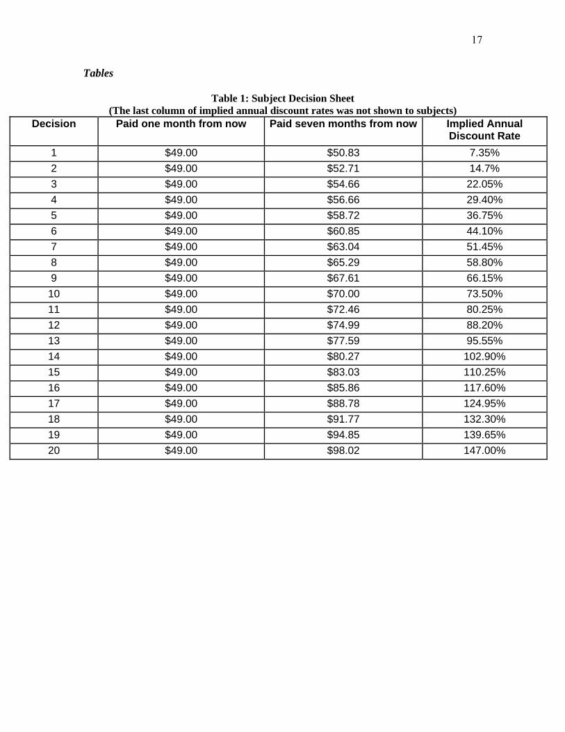
In the experiment, students are asked to make twenty decisions. For each

decision, students are asked if they would prefer $49 one month from now or $49+$X six

months from now. The amount of money, $X, is strictly positive and increases over the

twenty decisions. The decision sheet that the subject sees is shown in Table 1 without the

last column indicating the implied annual discount rate.

To administer the experiment, the subjects are divided into classrooms, so there

are roughly 25 subjects in each room. In each room, subjects are assigned a unique

identification code. This code is private, and subjects do not know the identification

codes of other subjects. Subjects make their decisions by circling one amount, either $49

or $49+$X, on their decision sheet. After subjects make their decisions, each subject puts

his decision sheet in an envelope and the envelopes are collected. All the envelopes are

shuffled in front of the subjects, and four envelopes per room are chosen for payment.

The identification codes of these chosen subjects are written on the blackboard. Because

identification codes are kept private by each subject, no subject knows the identity of the

subjects chosen to receive payment.

One decision out of the twenty decisions is randomly chosen for payment. This is

done by taking 20 index cards with the numbers 1-20 written on them, shuffling them in

front of the subjects, and asking a subject to choose one card. The number on the card is

the decision number to be paid for each of the four subjects who are chosen to receive

9

payment. So, for example, if decision number 15 is chosen for payment, and a winning

subject had circled $83.03 for this decision, then the subject would receive $83.03 six

months from now. If another subject circled $49, that subject would receive $49 on one

month from now.

Subjects who are chosen to receive payment are paid with a Wal-Mart gift card by

the school principal on the specific date for the decision chosen. The school principal

keeps the Wal-Mart gift cards in her office and the names of the subjects who are chosen

for payment. Within a week of the experiment, the subject is asked to stop by the

principal’s office to verify winning the gift card. On the date of payment, the subject is

invited to come privately to the principal’s office on or within a week of the date to pick

up the gift card. For the subjects chosen to be paid, their names and the amount of

payment are kept private. Subjects knew all of these procedures before making their

decisions.

Economic theories of discounting predict that an individual faced with the

decision sheet in Table 1 would either choose (a) $49 for all decisions, (b) the higher

payment for all decisions, or (c) $49 for a certain number of decisions starting with

Decision 1 and then switch to the higher payment for the remaining decisions. In other

words, if an individual chose to receive $Y in seven months rather than $49 in one

month, then the individual will prefer any amount $Z > $Y in seven months rather than

$49 in one month. Following Harrison et al. (2002), we call these individuals “consistent”

decision-makers (Bettinger and Slonim called them “rational”).

However, in experiments using decision sheets like the one in Table 1, some

individuals are “inconsistent” decision-makers: they choose $Y in seven months rather than

$49 in one month, but then choose $49 in one month rather than $Z>$Y in seven months.

Harrison et al. (2002) and Meier and Sprenger (2006) found that 4% and 11%, respectively,

10

of their adult subjects were inconsistent in their choices. Bettinger and Slonim (2007), whose

subjects were between 5 and 16 years old, found that 34% of their sample were inconsistent

decision-makers. A method to deal with inconsistent decision-makers is described below.

The experiments were conducted with 8th graders at two middle schools.

Nationally, 35 percent of students who drop-out of school do so between the ninth and

tenth grades. Thus, it is in that transition from middle to high school (beginning in eighth

grade) that the impatience of students may be most relevant for educational outcomes.

4. Experiment Results

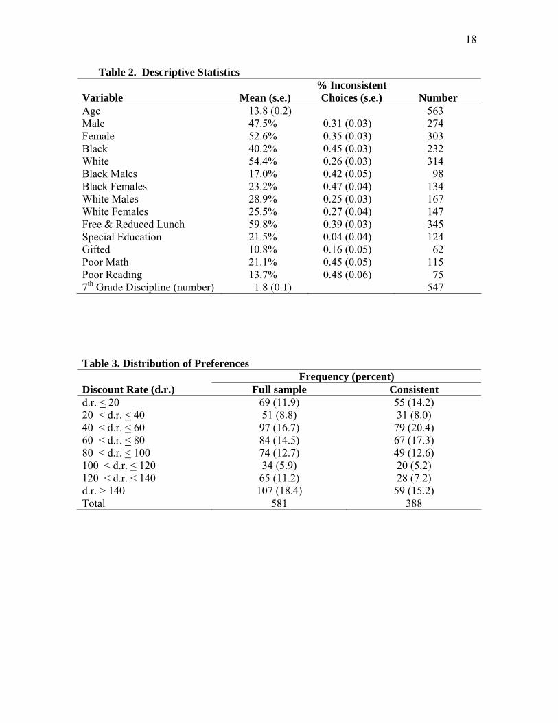
Table 2 shows descriptive statistics for the population of students in the

experiment. Forty-seven percent of the subjects are male and 40.2% are Black. Almost

60% of the children receive free or reduced price lunch and 21.5% are part of a special

education program. According to their 7th grade aptitude test, 21.1% of the children do

not satisfy the math requirement for their grade and 13.7% do not satisfy the reading

requirements.

Table 2 also shows the proportion of kids that make at least one inconsistent

decision in the experiment. Sixty-seven percent of the subjects make consistent decisions

and less than 10 percent make five or more inconsistent decisions. The distribution of

inconsistent behavior is not distributed randomly. Black subjects are more likely to

behave inconsistently. Gifted children are the least likely to make inconsistent decisions,

and children with reading deficiencies are the most likely to make inconsistent decisions,

followed by children with math deficiencies. Table 3 presents the distribution of discount

rates for all the subjects and only for subjects that answered consistently. The discount

rate of inconsistent subjects is estimated by finding the distribution of choices that is

consistent and minimizes the total amount of money that would have to be spent to adjust

their behavior. Let xij be the amount of money child i chooses from menu j and let X be

11

the set of all possible consistent patterns of behavior. Our estimates for inconsistent

children are based on the ^x such that ∑ −= ∈ j jijXx xxx minarg

^.

5. Family Survey

After conducting the experiments among the eighth graders in the two middle

schools, they were asked to take a family survey home to be filled out by their parent or

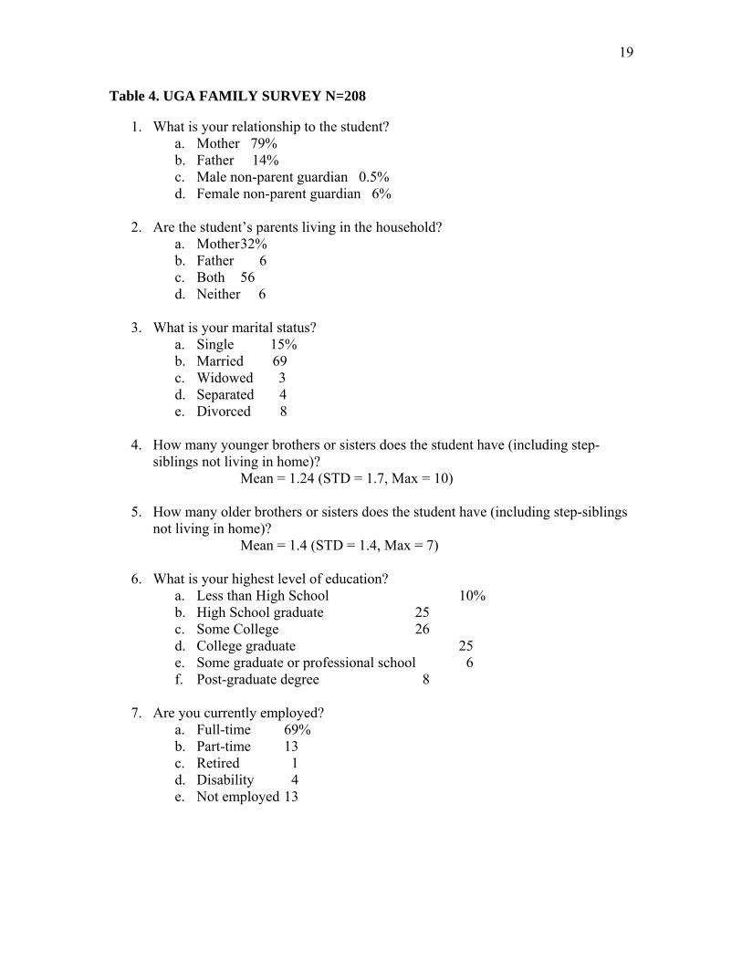
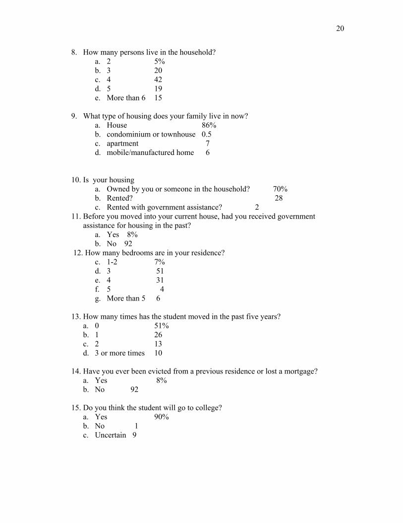
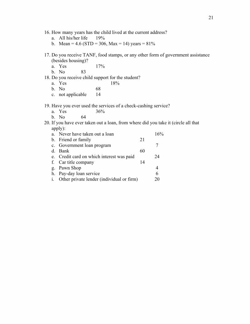
guardian (table 4). The short (20 questions) survey was designed to explore some of the

factors that may have an impact on children’s time preferences. These included the

relationship of adults in the household to the student, birth order, educational and

employment status of the parent or guardian, expectations of higher education, existence

of government assistance and child support, and proxy questions regarding financial

management. Seven of the twenty questions were about the housing conditions of the

family. These housing questions are used in the analysis for this paper.

Just over one-third of the students lived in a household where over four person

live. Most (86%) live in a house and 70% are owned by someone in the household. Only

8% of the families had received government assistance for housing. Half of the

respondents said their house has 3 bedrooms, and 41% have more. Seventy-six percent of

the students had moved either once or not a all in the past five years and only 8% had

ever been evicted. Overall, the housing situation of these students appears stable.

6. Results

In this paper we use the probit model of probability of being impatient:

Prob(Y) = X'b + H'c + S'd + ε

Where Y is a dummy variable which is constructed by using student impatience as

measured by the experimental discount rate, X is a set of family characteristics posited to

affect student impatience and, H is a vector of housing characteristics also hypothesized

12

to affect the time preference of students, S is a set of student characteristics, and b, c, and

d are coefficients, and ε is the stochastic error component. We use a probit model with

the discount rate equal to 0 if the computed discount rate is under .8 and 1 if it is over .8.

We use .8 as the midpoint in calculated discount rates over the 20 decisions as shown in

table 1. The X' vector of family characteristics include if both parents live in the

household, if the student has an older or younger sibling, if the parent has more than a

high school education, if the parent is employed, if the parent expects the student to

attend college, if the family receives child support, if they receive government assistance,

and if they use short-term financial tools such as check-cashing services, car title

companies, pawnshops or pay-day loan services. The H' vector of housing characteristics

include if there are four or less people in the house, if the family lives is a single-family

house, if they own the house, if the house has 3 or more bedrooms, if they did not move

in the last five years, if they received government housing assistance in the past, and if

they had ever been evicted. The S' vector is a set of student characteristics including

gender, race, income (whether the student is on a free or reduced lunch) instructional

setting (regular education, special education, gifted, remedial), standardized test scores in

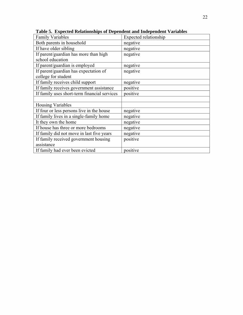
math and reading, number of discipline referrals, and number of absences. Table 5 shows

the expected relationships between student discount rates and the explanatory variables.

A negative relationship means the variable contributes to a more patient student and a

positive relationship shows those variables that may cause more impatience in a student.

We expect that a student living in a household with both parents, where at least one has

more than an high school education, is employed and expects the child to attend college

would create a situation where the student is patient, or less impatient. We also expect

the existence of an older sibling would affect patience. Although a family receiving child

13

support suggests a single-parent household, we expect a negative effect on impatience

since child support adds to family income and at least in a minimal sense suggests both

parents are involved in the life of the child. We expect families that receive government

assistance or use short-term financial tools will have a positive effect on impatience.

In terms of the housing characteristics, we expect that a child living in a less

crowed house that is owned by the family and has three or more bedrooms would have a

negative effect on the students discount rate, along with the fact that the family has not

moved in the last five years. If the family receives government housing assistance or has

been evicted from a home in the past is expected to have positive effect on child discount

rates. We have no apriori assumptions on the expected relationships between discount

rate and student characteristics.

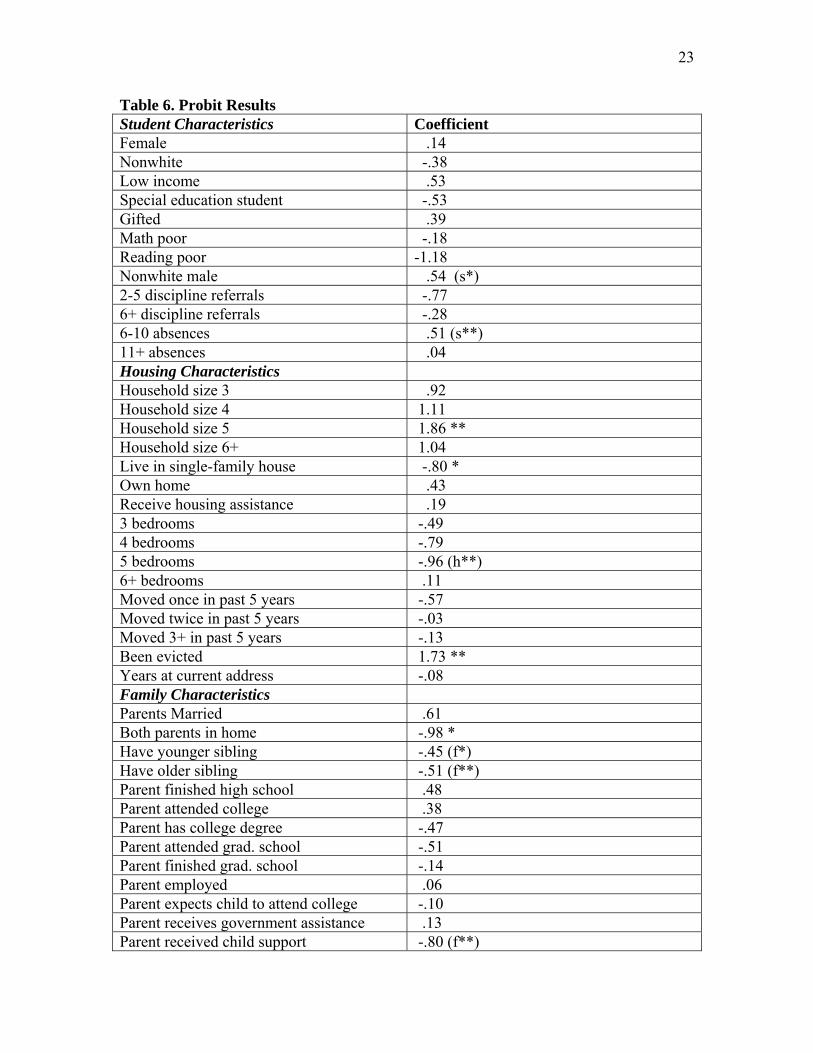
Of the 208 students for which there is experiment data, 165 returned the

family survey. The results of the full probit regression (Table 6) show that the

explanatory variables that were significant and negative included that both parents live at

home and they lived in a single-family dwelling. These variables had the effect of

reducing the child’s discount rate. The variables that were significant and positive

included household size of five and whether the family had ever been evicted from a

home, thus increasing child impatience. All of these were of the expected sign. All other

variables in the full model were insignificant. None of the variables that related to the

students’ school performance or situation were significant. We also ran separate probit

regressions for student, housing and family characteristics. Each of the four variables

above remained significant and of the correct sign. For student characteristics, being a

nonwhite male increased the discount rate and having 6-10 absences also increased the

discount rate. For the housing characteristics, the only additional variable that become

14

significant (and negative) when run separately was house size of five bedrooms. For

family characteristics, having either younger or older siblings as well as receiving child

support was also significant and negative.

7. Discussion and Conclusion

The reality of today’s housing market crises seems to confront the findings of

several studies that look into the benefits of homeownership. These studies propose that

the main arguments for homeownership are not primarily economic, but social. For

example, homeownership benefits society because it encourages stable, more law-abiding

communities; it makes people more likely to vote in local elections and join clubs; and it

benefits future generations because the children of homeowners do better at school and

have fewer behavioral problems than children of renters (Green and White, 1997;

DiPasquale and Glaeser, 1998; Hanushek, Kain and Rivkin, 1999). In general, research

supports the view that homeownership and stable housing bring substantial social

benefits. Some even argue that because of these extensive social benefits government

assistance and subsidies for the housing industry are well justified.

However, studies that examine social benefits of homeownership on children

outcomes are required to account for a strong correlation between homeownership with

parental incomes, education, age, marital status, and several other factors. Therefore, a

strong correlation between homeownership and social outcome variables may merely be

superfluous in that the correlation is simply capturing the impact of higher income,

education, and the like. To isolate the impact solely attributable to homeownership and/or

stable housing, it is important to control for factors that are generally present with

homeownership (like higher income and older age). Policy makers will only then better

15

appreciate the challenges of encouraging and promoting people into homeownership and

providing stable housing.

In this paper we began with the hypothesis that students who face housing

uncertainties through mortgage foreclosures and eviction learn impatient behavior and are

therefore at greater risk of dropping out of school, impeding human capital formation and

community development. To test this hypothesis we incorporated the results of a parent

survey which covers the family housing situation and family characteristics with

experimental data on the time preferences of 8th grade students. We found that large

household size and the occurrence of an eviction significantly increases the discount rates

of children while living in a single-family home with both parents significantly deceases

child discount rates, and thus impatience. In addition nonwhite males and those who are

often absent from school also have higher discount rates than others while children who

live in large houses, have older and younger siblings as have income generated from

child support payments have lower discount rates as exhibited in the experiments.

The negative relationship between housing equity (5 bedroom homes) and living

with both parents, and discount rate shows the beneficial effect of the family’s financial

stability on the time preference of children. Since income shocks may have less damaging

consequences for families with greater housing equity, as parents are better able to cope

with the family tensions resulting from the temporary financial troubles that the family

faces and thus are able to remain together and avoid significant income losses from

divorce or separation. The results of this study are consistent with the findings from Zhan

and Sherraden (2003) study which find that parental asset ownership improved the

educational outcomes for children.

16

One possible limitation of projects that support homeownership in poor

neighborhoods is the danger that these same programs may also encourage some low

income households to own homes even though they may not be able to sustain the

necessary mortgage payments across time. Extant research shows that a high rate of

mortgage default and foreclosure has a detrimental effect on the property values and the

social capital of the neighborhood (Immergluck and Smith, 2004). However, pre- and

post-purchase counseling of at risk homeowners can reduce foreclosure and default rates

in a neighborhood significantly (Quercia, Cowan, and Moreno, 2004). Hence, for

successful gentrification of a neighborhood without the displacement, it is necessary to

identify the determining characteristics of at risk homeowners, who may need counseling

before and after purchase in order to sustain their homeownership.

17

Tables

Table 1: Subject Decision Sheet (The last column of implied annual discount rates was not shown to subjects)

Decision Paid one month from now Paid seven months from now Implied Annual Discount Rate

1 $49.00 $50.83 7.35% 2 $49.00 $52.71 14.7% 3 $49.00 $54.66 22.05% 4 $49.00 $56.66 29.40% 5 $49.00 $58.72 36.75% 6 $49.00 $60.85 44.10% 7 $49.00 $63.04 51.45% 8 $49.00 $65.29 58.80% 9 $49.00 $67.61 66.15% 10 $49.00 $70.00 73.50% 11 $49.00 $72.46 80.25% 12 $49.00 $74.99 88.20% 13 $49.00 $77.59 95.55% 14 $49.00 $80.27 102.90% 15 $49.00 $83.03 110.25% 16 $49.00 $85.86 117.60% 17 $49.00 $88.78 124.95% 18 $49.00 $91.77 132.30% 19 $49.00 $94.85 139.65% 20 $49.00 $98.02 147.00%

18

Table 2. Descriptive Statistics Variable

Mean (s.e.)

% Inconsistent Choices (s.e.)

Number

Age 13.8 (0.2) 563 Male 47.5% 0.31 (0.03) 274 Female 52.6% 0.35 (0.03) 303 Black 40.2% 0.45 (0.03) 232 White 54.4% 0.26 (0.03) 314 Black Males 17.0% 0.42 (0.05) 98 Black Females 23.2% 0.47 (0.04) 134 White Males 28.9% 0.25 (0.03) 167 White Females 25.5% 0.27 (0.04) 147 Free & Reduced Lunch 59.8% 0.39 (0.03) 345 Special Education 21.5% 0.04 (0.04) 124 Gifted 10.8% 0.16 (0.05) 62 Poor Math 21.1% 0.45 (0.05) 115 Poor Reading 13.7% 0.48 (0.06) 75 7th Grade Discipline (number) 1.8 (0.1) 547 Table 3. Distribution of Preferences Frequency (percent) Discount Rate (d.r.) Full sample Consistent d.r. < 20 69 (11.9) 55 (14.2) 20 < d.r. < 40 51 (8.8) 31 (8.0) 40 < d.r. < 60 97 (16.7) 79 (20.4) 60 < d.r. < 80 84 (14.5) 67 (17.3) 80 < d.r. < 100 74 (12.7) 49 (12.6) 100 < d.r. < 120 34 (5.9) 20 (5.2) 120 < d.r. < 140 65 (11.2) 28 (7.2) d.r. > 140 107 (18.4) 59 (15.2) Total 581 388

19

Table 4. UGA FAMILY SURVEY N=208 1. What is your relationship to the student?

a. Mother 79% b. Father 14% c. Male non-parent guardian 0.5% d. Female non-parent guardian 6%

2. Are the student’s parents living in the household? a. Mother 32% b. Father 6 c. Both 56 d. Neither 6

3. What is your marital status? a. Single 15% b. Married 69 c. Widowed 3 d. Separated 4 e. Divorced 8

4. How many younger brothers or sisters does the student have (including step-siblings not living in home)?

Mean = 1.24 (STD = 1.7, Max = 10)

5. How many older brothers or sisters does the student have (including step-siblings not living in home)?

Mean = 1.4 (STD = 1.4, Max = 7) 6. What is your highest level of education?

a. Less than High School 10% b. High School graduate 25 c. Some College 26 d. College graduate 25 e. Some graduate or professional school 6 f. Post-graduate degree 8

7. Are you currently employed? a. Full-time 69% b. Part-time 13 c. Retired 1 d. Disability 4 e. Not employed 13

20

8. How many persons live in the household? a. 2 5% b. 3 20 c. 4 42 d. 5 19 e. More than 6 15

9. What type of housing does your family live in now? a. House 86% b. condominium or townhouse 0.5 c. apartment 7 d. mobile/manufactured home 6

10. Is your housing a. Owned by you or someone in the household? 70% b. Rented? 28 c. Rented with government assistance? 2

11. Before you moved into your current house, had you received government assistance for housing in the past?

a. Yes 8% b. No 92

12. How many bedrooms are in your residence? c. 1-2 7% d. 3 51 e. 4 31 f. 5 4 g. More than 5 6

13. How many times has the student moved in the past five years? a. 0 51% b. 1 26 c. 2 13 d. 3 or more times 10

14. Have you ever been evicted from a previous residence or lost a mortgage?

a. Yes 8% b. No 92

15. Do you think the student will go to college?

a. Yes 90% b. No 1 c. Uncertain 9

21

16. How many years has the child lived at the current address? a. All his/her life 19% b. Mean = 4.6 (STD = 306, Max = 14) years = 81%

17. Do you receive TANF, food stamps, or any other form of government assistance

(besides housing)? a. Yes 17% b. No 83

18. Do you receive child support for the student? a. Yes 18% b. No 68 c. not applicable 14

19. Have you ever used the services of a check-cashing service?

a. Yes 36% b. No 64

20. If you have ever taken out a loan, from where did you take it (circle all that apply): a. Never have taken out a loan 16% b. Friend or family 21 c. Government loan program 7 d. Bank 60 e. Credit card on which interest was paid 24 f. Car title company 14 g. Pawn Shop 4 h. Pay-day loan service 6 i. Other private lender (individual or firm) 20

22

Table 5. Expected Relationships of Dependent and Independent Variables Family Variables Expected relationship Both parents in household negative If have older sibling negative If parent/guardian has more than high school education

negative

If parent/guardian is employed negative If parent/guardian has expectation of college for student

negative

If family receives child support negative If family receives government assistance positive If family uses short-term financial services positive Housing Variables If four or less persons live in the house negative If family lives in a single-family home negative It they own the home negative If house has three or more bedrooms negative If family did not move in last five years negative If family received government housing assistance

positive

If family had ever been evicted positive

23

Table 6. Probit Results Student Characteristics Coefficient Female .14 Nonwhite -.38 Low income .53 Special education student -.53 Gifted .39 Math poor -.18 Reading poor -1.18 Nonwhite male .54 (s*) 2-5 discipline referrals -.77 6+ discipline referrals -.28 6-10 absences .51 (s**) 11+ absences .04 Housing Characteristics Household size 3 .92 Household size 4 1.11 Household size 5 1.86 ** Household size 6+ 1.04 Live in single-family house -.80 * Own home .43 Receive housing assistance .19 3 bedrooms -.49 4 bedrooms -.79 5 bedrooms -.96 (h**) 6+ bedrooms .11 Moved once in past 5 years -.57 Moved twice in past 5 years -.03 Moved 3+ in past 5 years -.13 Been evicted 1.73 ** Years at current address -.08 Family Characteristics Parents Married .61 Both parents in home -.98 * Have younger sibling -.45 (f*) Have older sibling -.51 (f**) Parent finished high school .48 Parent attended college .38 Parent has college degree -.47 Parent attended grad. school -.51 Parent finished grad. school -.14 Parent employed .06 Parent expects child to attend college -.10 Parent receives government assistance .13 Parent received child support -.80 (f**)

24

References

Aaronson, D. 2000. "A Note on the Benefits of Homeownership." Journal of Urban Economics, 47: 356-69. Astone, N.M., & S.S. McLanahan. 1991. “Family Structure, Parental Practices and High School Completion.” American Sociological Review, 56:309-302. Ausubel, L. M. 1991. “The Failure of Competition in the Credit Card Market.” American Economic Review, 81(1):51-81 Becker, G. S., and C. B. Mulligan. 1997. “The Endogenous Determination of Time Preference.” Quarterly Journal of Economics, 112 (3): 729-58. Benzion, U., A. Rapoport, and J. Yagil. 1989. “Discount Rates Inferred from Decisions: an Experimental Study.” Management Science, 35: 270-284. Bettinger, E. and R. Slonim. 2007. “Patience Among Children.” Journal of Public Economics, 91(1-2): 343-363. Boehm, T. P. and A. Schlottmann. 1999. “Does Home Ownership by Parents Have an Economic Impact on Their Children?” Paper presented at the American Real Estate and Urban Economics Association Mid Year Meeting, New York, NY. Bowles, S., Gintis, H., and M. Osborne, 2001. “Incentive-Enhancing Preferences: Personality, Behavior and Earnings.” American Economic Review, 91(2): 155–158 Bowles, S., H.Gintis, and M.Osborne. 2002. “The Determinants of Individual Earnings: Skills, Preferences, and Schooling.” Journal of Economic Literature. December, 39(4): 137–176. Boyle, M. H. 2002. “Home Ownership and the Emotional and Behavioral Problems of Children and Youth.” Child Development, 73: 883 – 892. Bradford D., J. Zoller, and G. Silvestrii. 2004. “Estimating the Effect of Individual Time Preferences on the Demand for Preventative Health Care.” CHEPS Working Paper 007-04, March. Castillo, M., P. Ferraro, J.L. Jordan, and R. Petrie. 2008. “The Today and Tomorrow of Kids: Time Preferences and Student Performance.” Paper presented at the Southern Economic Association Annual Meeting, New Orleans, LA. Coller, M. and M.B. Williams. 1999. “Eliciting Individual Discount Rates.” Experimental Economics, 2(2): 107-127. Currie, J. and A. Yelowitz. 2000. “Are Public Housing Projects Good for Kids?” Journal of Public Economics, 75: 99–124.

25

Curtis, J. 2002. “Estimates of Fishermen's Personal Discount Rate.” Applied Economics Letters, 9(12): 775-78 DiPasquale, D, and E Glaeser. 1999. “Incentives and Social Capital: Are Homeowners Better Citizens?” Journal of Urban Economics, 45:354–84. Downey, D. 1995. “When Bigger is Not Better: Number of Siblings, Parental Resources, and educational Performance,” American Sociological Review, 60: 746–761. Eckel, C., C. Johnson and C. Montmarquette. 2005. “Human Capital Investment by the Poor: Calibrating Policy with Laboratory Experiments.” Working Paper. Frederick, S., G. Lowenstein & T. O’Donoghue. 2002. "Time Discounting and Time Preference: A Critical Review." Journal of Economic Literature, 40: 351-401 Gould, E.I. and M. A. Turner 1997. “Does Neighborhood Matter? Assessing Recent Evidence.” Housing Policy Debate, 8(4): 833-866. Gately, D. 1980. “Individual Discount Rates and the Purchase and Utilization of Energy-using Durables: Comment.” Bell Journal of Economics, 11: 373-374. Galster, G. C. 1987. Homeowners and Neighborhood Reinvestment. Durham, NC: Duke University Press. Green, R, and M White. 1997. "Measuring the Benefits of Homeowning: Effects on Children." Journal of Urban Economics, 41: 441-61. Gyourko, J., & P. Linneman 1999. “The Changing Influences of Education, Income, Family Structure, and Race on Homeownership by Age Over Time.” Journal of Housing Research. 8(1): 1-25. Hanushek, E., J. Kain, and S. Rivkin. 2004. “Disruption vs. Tiebout Improvement: The Costs and Benefits of Switching Schools.” Journal of Public Economics, 88:1721–46. Harkness, J. and S. J. Newman, 2002. “Homeownership for the Poor in Distressed Neighborhoods: Does This Make Sense?” Housing Policy Debate, 13: 597-630. Harrison, G.W., M. Lau and M. Williams. 2002. “Estimating Individual Discount Rates for Denmark: A Field Experiment.” American Economic Review, 92(5): 1606-1617. Hartman, R. S., and M. J. Doane. 1986. “Household Discount Rates Revisited.” The Energy Journal, 7: 139-48. Haurin, Donald, Toby Parcel, and R. Jean Haurin. 2002a. “Does Home Ownership Affect Child Outcomes?” Real Estate Economics, 30:635–66. Haurin, Donald, Toby Parcel, and R. Jean Haurin. 2002b. “Impact of Home Ownership on Child Outcome.” In Low Income Homeownership: Examining the Unexamined Goal,

26

ed. Eric S. Belsky and Nicolas P. Retsinas, 427–46. Washington, DC: Brookings Institu-tion Press. Haurin, D.R., R.D. Dietz and B.A. Weinberg 2003. “The Impact of Neighborhood Homeownership Rates: A Review of Theoretical and Empirical Literature?” Real Estate Economics, 30(4): 635–66. Hausman, J.A, 1979. “Individual Discount Rates and the Purchase and Utilization of Energy-Using Durables.” Bell Journal of Economics, 10: 33-54. Haveman, R., B. Wolfe, and J. Spaulding. 1991. “Childhood Events and Circumstances Influencing High-School Completion.” Demography, 28(1): 133-57. Holcomb, J.H. and P.S. Nelson. 1992. “Another Experimental Look at Individual Time Preference.” Rationality and Society, 4: 199–220. Immergluck, D., and G. Smith 2004. There Goes the Neighborhood: The Effect of Single-Family Mortgage Foreclosures on Property Values. Chicago, IL: Woodstock Institute. Kauppinen, T. 2004. “Neighbourhood Effects in a European City: The Educational Careers of Young People in Helsinki.” Paper presented at the meeting of the European Network for Housing Research, Cambridge, England. Lovell, P. and J. Isaacs, 2008. “The Impact of the Mortgage Crisis on children and Their Education. First Focus, (April) 1-5. Lowenstein, G.F. 1988. “Frames of Mind in Intertemporal Choice.” Management Science 34: 200–214. Marcuse, P. 1989. “Gentrification, homelessness, and the Work Process: Housing Markets and Labour Markets in the Quartered City.” Housing Studies. 4(3): 211-220. McCarthy, G., S. Van Zandt and W.M. Rohe. June 2001. The Economic Benefits and Costs of Homeownership: A Critical Assessment of the Research. Washington, DC: Research Institute for Housing America. Meier, S. and C. Sprenger. 2006. “Impatience and Credit Behavior: Evidence from a Field Experiment. Working Paper, October. Northwest Venture Communities Inc. 2003. Dakota Dreams: Partnering for Prosperity, a Ten-year Plan to Reduce Poverty in Northwest North Dakota. Minot, ND: Northwest Venture Communities Inc. Pender, J.L. 1996. “Discount Rates and Credit Markets: Theory and Evidence from Rural India.” Journal of Development Economics, 50: 257–296. Quercia, R. G., S.M. Cowan., and A. Moreno. 2004. “The Cost-Effectiveness of Community-Based Foreclosure Prevention.” Joint Center for Housing Studies Working

27

Paper Series, BABC, 04-18. Rohe, W.M., S. Van Zandt and G. McCarthy. 2002. "Home Ownership and Access to Opportunity: A Review of the Research Evidence." Housing Studies, 17(1), 51-61. Rossi, P H., and E. Weber. 1996. "The Social Benefits of Homeownership: Empirical Evidence from National Surveys." Housing Policy Debate, 7(1): 1-35. Ruderman, H., M. Levine, and J. McMahon. 1986. “Energy Efficiency Choice in the Purchase of Residential Appliances.” In Energy Efficiency: Perspectives on Individual Behavior, W. Kempton and M. Neiman, eds. American Council for an Energy Efficient Economy, pp. 41-50. Samuelson, P. (1937). “A Note on Measurement of Utility” Review of Economic Studies, 4(2): 155-161. Shelley, M.K. 1993. “Outcome Signs, Question Frames and Discount Rates.” Management Science, 39: 806–815. Thaler, R. H. 1981. “Some Empirical Evidence on Dynamic Inconsistency.” Economics Letters, 8: 201-207. Tinsley, K. 2005. Housing Stress Counties in Georgia. UGA: Housing and Demographics Research Center. Warner, J. T. and S. Pleeter. 2001. “The Personal Discount Rate: Evidence from Military Downsizing Programmes. American Economic Review, 91: 33-53. Zhan, M. and M.Sherraden. 2003. “Assets, Expectations and Educational achievement.” Social Service Review, 77(2): 191-211