1

How does ocean acidification impact phytoplankton productivity and community structure?

Aliza Ray1 and Joe Vallino

2

1Bard College, Annandale-On-Hudson NY 12504

2Marine Biological Laboratory, Ecosystem Center, Woods Hole MA 02543

2

Abstract

Increasing atmospheric CO2 concentration will result in the acidifying and CO2 fertilization of our

oceans. Phytoplankton assemblages will be among the organisms affected by theses changes. We

tested how coastal New England phytoplankton community photosynthetic productivity and

community composition will be changed. This microcosm experiment manipulated the CO2

concentrations to be 370µatm, 925µatm, and 3700µatm over a 3 week incubation period.

Treatments showed reduced pH and changed dissolved inorganic carbon levels relative to each

treatment. Measured parameters included nutrients, Chl a, pCO2, enumeration, and quantification

of phytoplankton taxa using microscopy and flow cytometry. The present study revealed a coastal

plankton community that was slightly affected by ocean acidification. Changes in respiration

across the course of a 24 hour period showed net consumption cycles to be greatest at elevated

CO2 levels. A species shift was seen from control treatments to elevated treatments and over a 5

day period. We have concluded that future research needs to be done to accurately determine how

phytoplankton will be affected by ocean acidification changes.

Key Words:

Ocean acidification, phytoplankton, primary productivity, community composition

Introduction

Elevated atmospheric CO2 levels, primarily due to fossil fuel combustion, has led to

increased CO2 fertilization of oceans (Brewer 2009), also known as ‘ocean acidification’.

Currently the atmospheric CO2 concentration is 390ppm, and is expected to increase to 750 ppm

or higher by the end of the century (Raven et al. 2005). Global elemental cycles are driven by

biological activity. Assessing the impact of ocean acidification on marine microorganisms is

important for understanding how aquatic systems will react. Observing microbe-driven

ecosystem function changes to elevated CO2 has proven challenging (Liu et al. 2010) and (Joint

et al. 2011).

Phytoplankton play an important role as primary producers of aquatic systems. Direct

effects between ocean acidification and photosynthetic ability have been observed to increase

under elevated pCO2 (Rost et al. 2008). The net rate of organic carbon production determines

support for higher trophic levels. Natural phytoplankton assemblages have been shown to

enhance photosynthesis under elevated pCO2 (Egge et al. 2009). This study will focus on coastal

phytoplankton community because they contribute significantly to global primary productivity

(Field et al. 1998).

Changes in community composition can also be caused by elevated pCO2. Global

changes in biodiversity can alter ecosystem services and disturb biogeochemical cycles, such as

control the CO2 taken up by the oceans. Different species play different roles in ecosystem

3

dynamics. For example, the size of phytoplankton determines grazing efficiencies and can alter

the population structure of grazers. Microbial community structure shifts can mean a loss of

biodiversity, compromised of ecosystem robustness, and potentially major consequences for

higher trophic levels. Studies that have observed the effects of increased CO2 inputs on

phytoplankton systems have found mixed results on phytoplankton assemblages (Nielsen et al.

2010). It is likely that different phytoplankton taxa react differently to ocean acidification. The

effects of elevated pCO2 on microzooplankton have shown no consistent effect to ocean

acidification on microbial biodiversity and community composition (Suffrian et al. 2008).

In the following we describe the responses of natural fall coastal phytoplankton groups to

changes in the carbonate chemistry of a microcosm system to determine how future lowered pH

levels and increased CO2 may alter functioning and composition. This study focuses on the

changes to phytoplankton photosynthetic productivity and community assemblages. To examine

the effects we created semi-continuous microcosm culture techniques in which CO2 manipulated

environments were periodically pulsed by pulling sampling and returning medium with nutrients

and filtered seawater. Here, we report on the results of a 3 week experiment demonstrating

effects of elevated CO2 levels of phytoplankton productivity on local North-west Atlantic Ocean

assemblages. We discuss the potential ecological and biogeochemical implications of our

findings.

Methods

A coastal seawater sample was obtained from Woods Hole, MA (41.5264° N, 70.6736°

W) during November. The sample was filtered through 200µm mesh. 1L of sample was allocated

to each microcosm with nutrients. Nutrient concentrations in the microcosms remained at 36µM

KNO3, 52µM NaSiO3, and 2.3µM KH2PO4. The experiment was preformed on triplicates at

925µatm, 3700µatm, and controlled atmospheric levels of 370µatm. Microcosms were incubated

at 20˚C on a 12 hour light cycle and were continuously stirred. CO2 and air input were bubbled

into the sample at 23 mL min-1

. Each day, 10% of the sample was removed and the same volume

of 0.45µm filtered seawater and nutrients were added back in. All air and water samples were

taken +/- 1 hour of growth lights turning on each day. The microcosms sat undisturbed for 4 days

prior to initiation of the pulse chemostat method.

4

10mL of sample was used to measure pH with Accumet pH/conductivity meter (Fisher

Scientific). 10mL was used for fluorescence using a Fluorometer (Turner Designs). 80mL of was

filtered using 25mm GF/F filters for nutrients. Ammonium was measured using a modification of

the phenol-hypochlorite method (Solorzano 1969) analyzed with a Cary UV Visible

Spectrophotometer (Varian). Phosphate was analyzed by a modification of the method of

Murphy and Riley (1962) using UV-VIS Spectrophotometer (Shimadzu). Nitrate was measured

using QuickChem Flow Injection Analyzer (LACHET). Filters were dried, and analyzed for

molar carbon and nitrogen with a PerkinElmer 2400 Series II CHN Elemental Analyzer.

10mL of sample was used to measure dissolved inorganic carbon levels. 20mL of

Ascarite scrubbed CO2-free air was drawn into the syringe, 0.2mL of H2SO4 was added, and

sample was shaken for 1 minute prior to injection of air. pCO2 in the microcosm head space and

CO2 input to the system was also measured. CO2 consumption was calculated by subtracting

pCO2 input from output, then multiplying by flow rate (23mL min-1

). Dissolved inorganic carbon

(DIC) and microcosm air was measured using gas chromatography (GC-8A Shimadzu).

50mL of sample was drawn for microscopy. Autotrophs were fixed in alkaline Lugol’s

solution (10g iodine, 20g potassium iodide, 10g sodium acetate, in 140ml distilled water) for a

concentration of 0.1%, followed by borate-buffered formalin addition of 2.4%, and 3% sodium

thiosulfate for a final concentration of 0.1% (Sherr and Sherr, 1993). Preserved sample were

filtered onto 25mm white 0.8µm membrane filters (Osmonics). Taxa were identified to the

nearest genus or species. Identification was done using differential interference and bright field

light microscopy (Zeiss Axio Imager.M2) at 20X and 40X.

Additional samples (50mL) were fixed to a final concentration of 5% glutaric dialdehyde.

Direct DAPI (4',6-diamino-2-phenylindole dihydrochloride) counts were taken from the

glutaraldehyde preserved samples. 1 ml of sample and 50µl of 200µg/ml working solution DAPI

was incubated for 5 minutes then drawn onto 1µm black polycarbonate filters. Phosphate

buffered saline was used to rinse. Samples were viewed under 20X magnification using blue

fluorescence. Samples were quantified:

cells ml-1 =(cells/field of view)´ (area of filter covered by sample)

(field of view area)´ (preseravtion dilution factor)´ (ml filtered)

Flow cytometry was done on live, unpreserved samples using a flow cytometer (BD

FACSCalibur) using CellQuest Pro software. 1mL samples were drawn and filtered using 35µm

5

mesh, and 5µL of 1µm beads were added to the sample. Particles were enumerated based on size,

complexity, and fluorescence.

Results

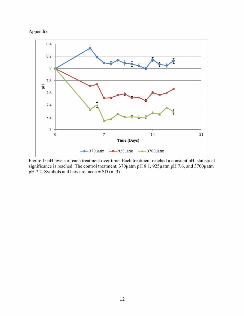
Measured pH during the experimental period remained constant once a steady pH was

reached (Figure 1). There were significant differences in pH between treatments. The 370µatm

(control) maintained a pH of 8.1, 925µatm was 7.6, and 3700µatm was 7.3. Seawater sampled at

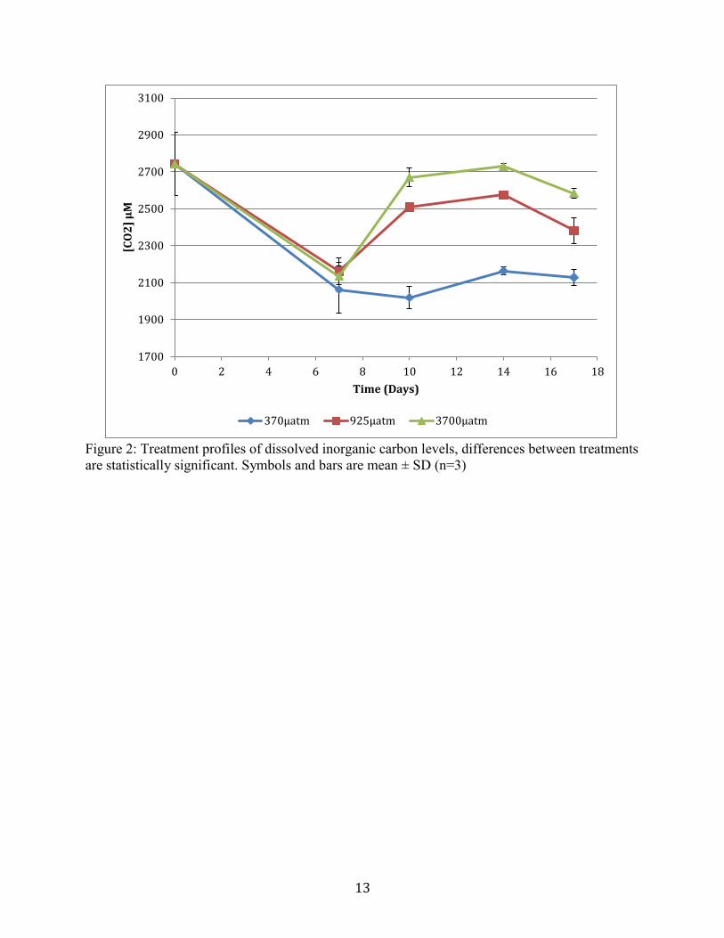
the start of the experiment measured a pH of 8. The initial level of DIC of the sampled water was

2700µM, and for all treatment levels the DIC changes occurred during the experimental period

(Figure 2).

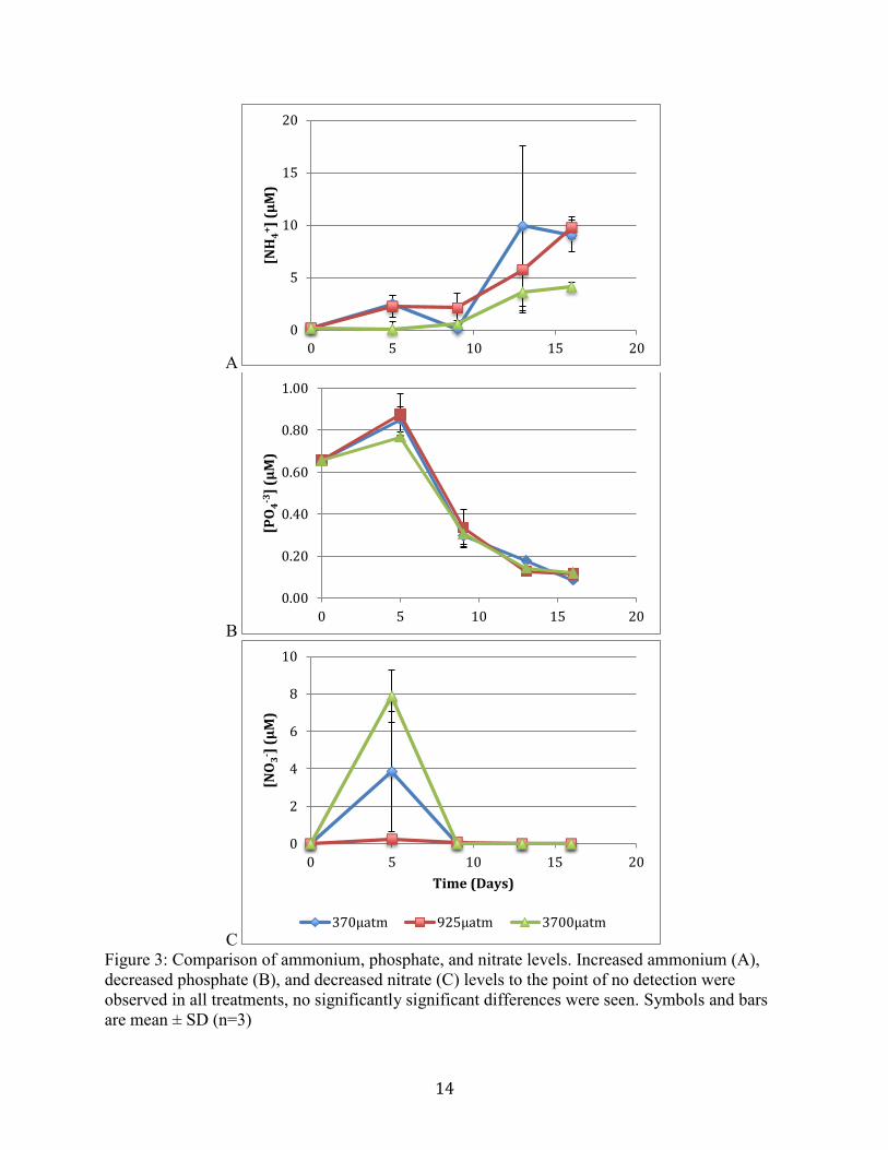
Nutrient profiles phosphate and ammonium were measured throughout the course of the

experiment. Initial concentrations of ammonium were undetectable, phosphate measured

0.66µM, and nitrate was also undetectable in the seawater sampled. Ammonium levels gradually

increased in all treatments over the course of the experiment (Figure 3A). Phosphate levels

gradually decreased in all treatments (Figure 3B). Levels of nitrate after day 5 were below

detection limit (Figure 3C). No statistically significant differences were found between

treatments.

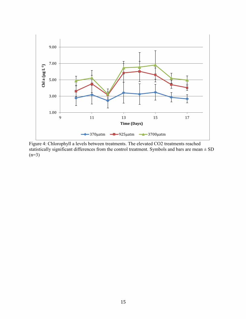
Chlorophyll a changes between treatments reflect changes based on treatment. Final Chl

a measurements reflect significant differences between treatments, with the 3700µatm treatment

having the highest Chl a values, and the ambient CO2 treatment measuring the lowest (Figure 4).

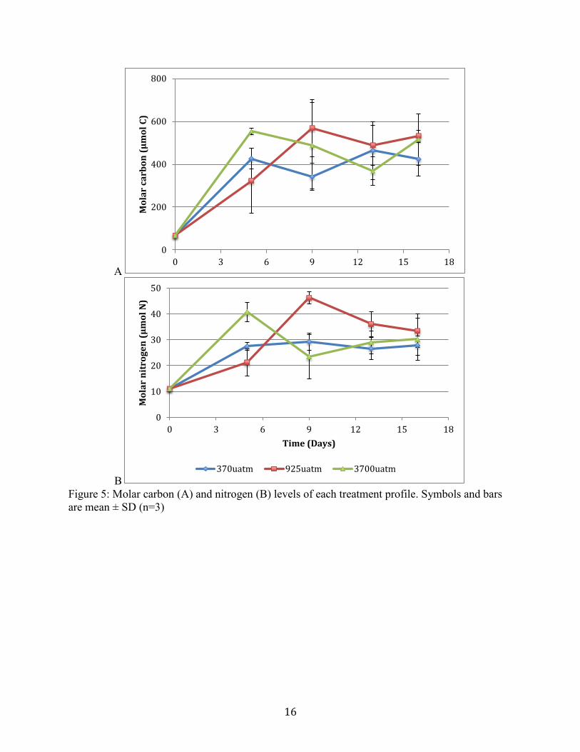
Molar carbon and nitrogen levels were not significant between treatments, all treatments showed

increasing fluctuation of C and N (Figure 5).

Measured carbon dioxide consumption showed significant difference between treatments.

Positive CO2 consumption values and slopes indicate net photosynthetic productivity, while

negative values and slopes indicate net CO2 production. Initial pCO2 values show net production,

while CO2(g) values after a 5 day acclimation period show increased consumption. Consumption

decreased in both elevated CO2 treatments. The control treatment reached a steady CO2

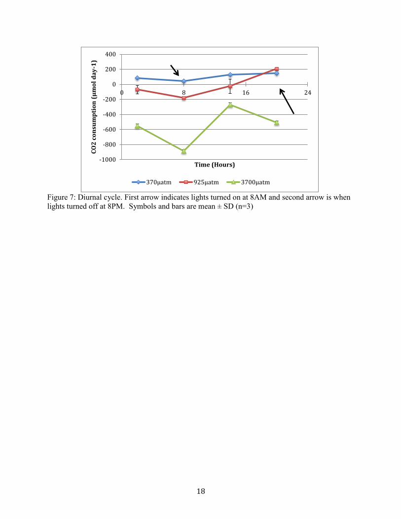
consumption rate (Figure 6). A diurnal pCO2 cycle shows significantly different consumption

values between treatments. Increased consumption is seen in each treatment during the 12 hours

the lights were on, except the highest CO2 treatment saw increased CO2 production from the

peak of midday until lights turn off at night. All treatments have negative consumption during

6

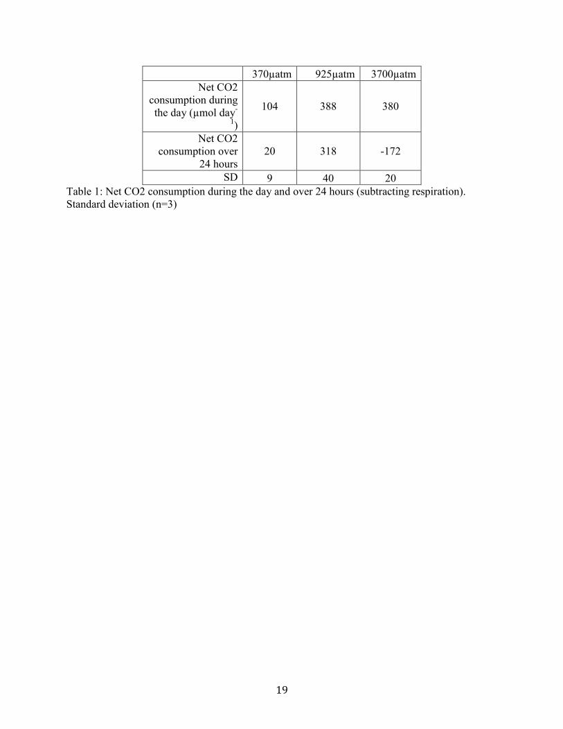
the 12 hours the lights were not on (Figure 7). Net CO2 consumption values due to

photosynthesis (during the period the lights were on) are increased from the 925µatm and

3700µatm treatments (Table 1). Net CO2 consumption during the course of 24 hours is negative

only for the 3700µatm treatment, meaning there is more CO2 produced than was consumed.

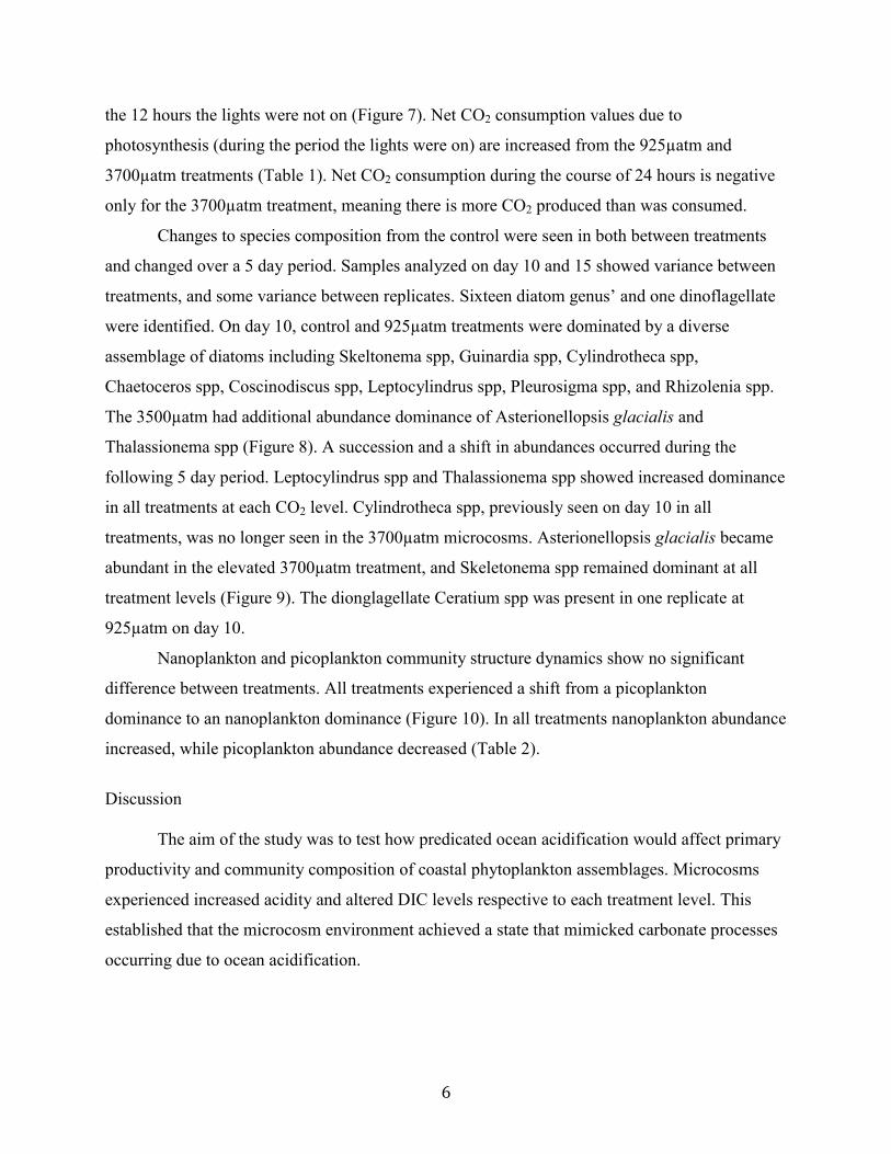
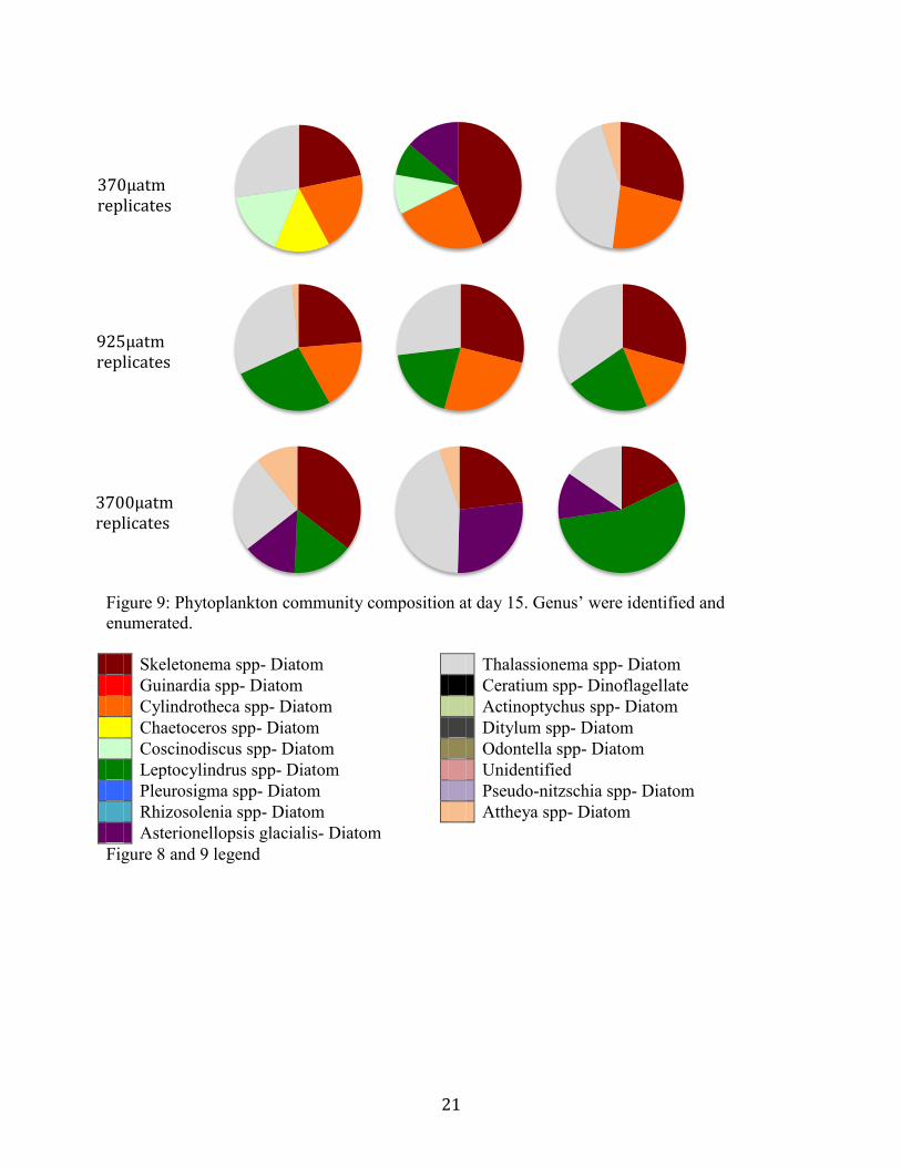
Changes to species composition from the control were seen in both between treatments

and changed over a 5 day period. Samples analyzed on day 10 and 15 showed variance between

treatments, and some variance between replicates. Sixteen diatom genus’ and one dinoflagellate

were identified. On day 10, control and 925µatm treatments were dominated by a diverse

assemblage of diatoms including Skeltonema spp, Guinardia spp, Cylindrotheca spp,

Chaetoceros spp, Coscinodiscus spp, Leptocylindrus spp, Pleurosigma spp, and Rhizolenia spp.

The 3500µatm had additional abundance dominance of Asterionellopsis glacialis and

Thalassionema spp (Figure 8). A succession and a shift in abundances occurred during the

following 5 day period. Leptocylindrus spp and Thalassionema spp showed increased dominance

in all treatments at each CO2 level. Cylindrotheca spp, previously seen on day 10 in all

treatments, was no longer seen in the 3700µatm microcosms. Asterionellopsis glacialis became

abundant in the elevated 3700µatm treatment, and Skeletonema spp remained dominant at all

treatment levels (Figure 9). The dionglagellate Ceratium spp was present in one replicate at

925µatm on day 10.

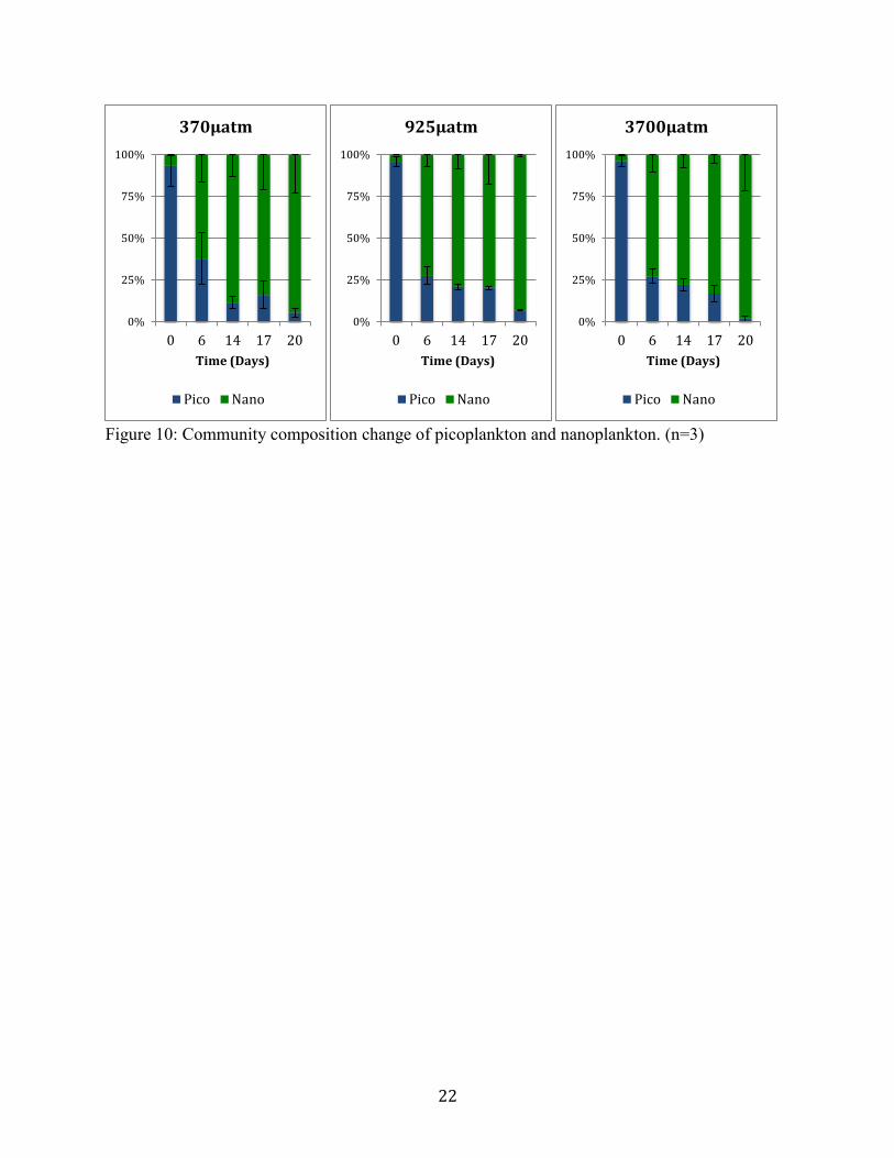
Nanoplankton and picoplankton community structure dynamics show no significant

difference between treatments. All treatments experienced a shift from a picoplankton

dominance to an nanoplankton dominance (Figure 10). In all treatments nanoplankton abundance

increased, while picoplankton abundance decreased (Table 2).

Discussion

The aim of the study was to test how predicated ocean acidification would affect primary

productivity and community composition of coastal phytoplankton assemblages. Microcosms

experienced increased acidity and altered DIC levels respective to each treatment level. This

established that the microcosm environment achieved a state that mimicked carbonate processes

occurring due to ocean acidification.

7

Despite relatively low nitrate levels, there was growth in the microcosms. Daily nitrate

additions of nutrient stock were enough to sustain growth, despite levels being undetectable 24

hours later.

Growth of phytoplankton in each treatment was observed. The initial drop in DIC over

the 5 day assimilation period occurred because of extreme growth in all treatments.

Photosynthetic carbon fixation causes a CO2 and DIC decrease. Phosphate levels decreased

significantly as well in all treatments, indicating growth, due to phosphate uptake. In addition,

Chlorophyll a levels of each treatment level had shown significant differences by the end of the

experiment.

Increased ammonium can mean more grazing on phytoplankton by larger zooplankton,

however, based on microcopy, no grazers were identified in any of the treatments. Nitrate uptake

by phytoplankton has been shown to inhibit by ammonium levels (l'Helguen et al. 2008).

Phytoplankton productivity, measured by the consumption of CO2, in all microcosms

increased during the first half of the experimental period. Decreased productivity in the elevated

CO2 treatments does not mean that consumption was not occurring, only that consumption was

lowered. Further examination of the carbonate chemistry of the systems would allow for

calculations of CO2(aq) in the water. The 24 hour diurnal cycle shows the fluctuations of CO2

consumption throughout the day. CO2 consumption is greatest in the elevated treatments. The

3700µatm treatment experienced net CO2 production during the course of 24 hours. When

photosynthesis was occurring during the lights on cycle, CO2 consumption occurs in all

treatments. CO2 consumption was greatest at the 3700µatm treatment level. Further works need

to be done to determine the CO2(aq) of the microcosms and carbonate chemistry changes to the

systems. Diatom dominated systems have shown 27% to 39% CO2 uptake increases from control

(~370µatm) (Riebesell et al. 2007).

Molar carbon level differences between treatments do not indicate elevated carbon

content at higher CO2 treatment levels. This could be due to carbon content difference based on

diversity of species seen.

The initial species dominance shift showed differences between treatments, primarily

diatoms. Resilience of Skeletonema spp in 3700µatm treatments was consistent with findings of

previous studies (Nielsen et al. 2012). The abundance of Asterionellopsis glacialis under

elevated CO2 was especially apparent. Individual phytoplankton physiology or nutrient

8

availability have not been closely assessed. Coastal phytoplankton communities have also been

observed to be impervious to CO2 elevated changes (Nielsen et al. 2010). While we acknowledge

the changes to species composition changes we saw, we also suggest that coastal phytoplankton

species could be tolerant of broad level pH fluctuations due to respiratory and photosynthetic

processes (Hansen 2002). Our phytoplankton may have been showing resilience to abrupt CO2

changes, previously seen (Vogt et al. 2008).

Flow cytometry results did not yield significant changes between treatment levels of

nanoplankton (2-20µm) and picoplankton (0.2-2µm) populations. Results were evidence of a

microcosm experiment, in which all treatments experienced a bottle-effect, in which

nanoplankton abundance increased, and picoplankton abundance decreased. Previous studies

have found only slight changes to picoplankton community composition under elevated CO2

levels (Newbold et al. 2012).

In a high CO2 ocean, phytoplankton may over-consume CO2, increasing their C:N ratio

(Toggweiler 1993). Elevated molar carbon level increased in all treatments, and the 925µatm and

3700µatm microcosm did not show significant differences in higher molar C compared to control

treatments. Increased CO2 and increased light have been found to decrease primary production at

light intensities representative of surface layer light levels (Gao et al 2012).

Further research on the effect of increasing CO2 levels on coastal, estuarine, and open-

ocean phytoplankton community assemblages. Our research is an example of one coastal

scenario. Both individual species effects and community productivity and resilience impacts

need to be further examined. Multiple environmental factors, such as nutrient level changes, need

to be examined in isolation of other variables, because of phytoplankton sensitivity to light and

nutrient levels. The ability of certain species to adapt to sudden pH changes is largely unknown.

It is important to study the impacts of ocean acidification to better understand its implications.

Acknowledgements

This exploration would not have been possible without the generosity of everyone at the

Marine Biological Lab. Joe Vallino for all his help, tremendous guidance, and carbonate

chemistry lessons. Hugh Ducklow, Matthew Erickson, Hap Garritt, and Ken Foreman for sharing

their lab and equipment. Jim McIlvain for endless Zeiss microcopy tutorials. Rich McHorney,

Alice Carter, and Carrie Harris for their endless patience.

9

Literature Cited

Brewer, P.G. 2009. A changing ocean seen with clarity. Proceedings of the National Academy of

Sciences USA, 106: 12213-14.

Field C.B., Behrenfeld, M.J., Randerson, J.T., Falkowski, P. 1998. Primary production of the

biosphere: integrating terrestrial and oceanic components. Science 281: 237-40.

Gao, K., Xu, J., Gao, G., Li, Y., Hutchins, D.A., Huang, B., Wang, L., Zheng, Y., Jin, P., Cai, X.,

Hader, D.P., Li, W., Xu, K., Liu, N., Ribesell, U. 2012. Rising CO2 and increased light

exposure synergistically reduce marine primary productivity. Nature Climate Change 2:

519-523

Hansen P.J. (2002) Effect of high pH on the growth and survival of marine phytoplankton:

implications for species succession. Aquatic Microbial Ecology 28: 79-88

Joing, I., Doney, S.C., Karl, D.M. 2011. Will ocean acidification affect marine microbes? The

ISME Journal, 5: 1-7.

Kemp, P.F., Cole, J.J., Sherr, B.F., Sherr, E.B., 1993. “Handbook of Methods in Aquatic

Microbial Ecology”. Lewis Publishers, Ann Arbor- Lugol’s protocol

L'Helguen, S., Maguer, J.F., Caradec, J. 2008. Inhibition kinetics of nitrate uptake by ammonium

in size-fractionated oceanic phytoplankton communities: implications for new production

and f-ratio estimates. Journal Plankton Research. 2008 30: 1179-1188

Lau, J., Weinbauer, M.G., Maier, C., Dai, M., Gattuso, J.P. 2010. Effect of ocean acidification on

microbial diversity and on microbe-driven biogeochemistry and ecosystem functioning.

Aquatic Microbial Ecology, 61: 291-305.

Murphy, J., Riley, J.P, 1962. A modified single solution method for the determination of

phosphate in natural waters. Analytica Chemica Acta 27: 31-6

Newbold, L.K., Oliver, A.E., Booth, T., Tiwari, B., DeSantis, T., Maguire, M., Andersen, G.,

van der Gast, C.J., Whiteley, A.S. 2012. The response of marine picoplankton to ocean

acidification. Environmental Microbiology 14(9): 2293-307

Nielsen, L.T., Jakobsen, H.H., Hansen, P.J. 2010. High resilience of two coastal plankton

communities to twenty-first century seawater acidification: evidence from microcosm

studies. Marine Biology Research: 6(6): 542-55

10

Nielsen, L.T., Hallegraeff, G.M., Wright, S.W., Hansen, P.J. 2012. Effects of experimental

seawater acidification on an estuarine plankton community. Aquatic Microbial Ecology

65: 271-85

Raven, J., Caldeira, K., Elderfield, H., Hoeg-Guldberg, O. 2005. Ocean acidification due to

increasing atmospheric carbon dioxide. Policy Document 12/05, The Royal Society,

London, available at: www.royalsoc.ac.uk

Riebesell, U., Schulz, K.G., Bellerby, R.G.J., Botros, M., Fritsche, P., Meyerhofer, M., Neill, C.,

Nondal, G., Oschlies, A., Wohlers, J., Zollner, E. 2007. Enhanced biological carbon

consumption in a high CO2 ocean. Nature, 450: 545-8.

Rost, B., Zondervan, I., Wolf-Gladrow, D. 2008. Sensitivity of phytoplankton to future changes

in ocean carbonate chemistry: current knowledge, contradictions and research directions.

Mar Ecological Progress Series, 373: 227-37.

Suffrian, K., Simonelli, P., Nejstgaard, J.C., Putzeys, S., Carotenuto, Y., Antia, A.N. 2008.

Microzooplankton grazing and phytoplankton growth in marine mesocosms with

increased CO2 levels. Biogeosciences Discussions 5: 411-433.

Solórzano, L. 1969. Determination of Ammonia in Natural Waters by the Phenol Hypochlorite

Method. Limnology and Oceanography 14.5: 799-801

Toggweiler, J.R. 1993. Carbon overconsumption. Nature 363: 210-11

Vogt, M., Steinke, M., Turner, S., Paulino, A., Meyerhofer, M., Riebesell, U., LeQuere, C. and

Liss, P. 2008. Dynamics of dimethylsulphoniopropionate and dimethylsulphide under

different CO2 concentrations during a mesocosm experiment. Biogeosciences 5: 407-419.

11

Figures and Tables

Figure 1. pH levels of each treatment over time. Each treatment reached a constant pH, statistical

significance is reached. The control treatment, 370µatm pH 8.1, 925µatm pH 7.6, and

3700µatm pH 7.2. Symbols and bars are mean ± SD (n=3)

Figure 2. Treatment profiles of dissolved inorganic carbon levels, differences between treatments

are statistically significant. Symbols and bars are mean ± SD (n=3)

Figure 3. Comparison of ammonium, phosphate, and nitrate levels. Increased ammonium (A),

decreased phosphate (B), and decreased nitrate (C) levels to the point of no detection

were observed in all treatments, no significantly significant differences were seen.

Symbols and bars are mean ± SD (n=3)

Figure 4. Chlorophyll a levels between treatments. The elevated CO2 treatments reached

statistically significant differences from the control treatment. Symbols and bars are mean

± SD (n=3)

Figure 5. Molar carbon (A) and nitrogen (B) levels of each treatment profile. Symbols and bars

are mean ± SD (n=3)

Figure 6. Treatment profiles of CO2 consumption. Positive values indicate consumption of CO2,

while negative values indicate CO2 production. Symbols and bars are mean ± SD (n=3)

Figure 7. Diurnal cycle. First arrow indicates lights turned on at 8AM and second arrow is when

lights turned off at 8PM. Symbols and bars are mean ± SD (n=3)

Table 1. Net CO2 consumption during the day and over 24 hours (subtracting respiration).

Standard deviation (n=3)

Figure 8. Phytoplankton community composition at day 10. Genus’s were identified and

enumerated.

Figure 9. Phytoplankton community composition at day 15. Genus’ were identified and

enumerated.

Figure 8 and 9 legend.

Figure 10. Community composition change of picoplankton and nanoplankton. (n=3)

Table 2. Changes in abundance of the nanoplankton and picoplankton population in each

treatment. (n=3)

12

Appendix

Figure 1: pH levels of each treatment over time. Each treatment reached a constant pH, statistical

significance is reached. The control treatment, 370µatm pH 8.1, 925µatm pH 7.6, and 3700µatm

pH 7.2. Symbols and bars are mean ± SD (n=3)

7

7.2

7.4

7.6

7.8

8

8.2

8.4

0 7 14 21

pH

Time (Days)

370µatm 925µatm 3700µatm

13

Figure 2: Treatment profiles of dissolved inorganic carbon levels, differences between treatments

are statistically significant. Symbols and bars are mean ± SD (n=3)

1700

1900

2100

2300

2500

2700

2900

3100

0 2 4 6 8 10 12 14 16 18

[CO

2]

µM

Time (Days)

370µatm 925µatm 3700µatm

14

A

B

C

Figure 3: Comparison of ammonium, phosphate, and nitrate levels. Increased ammonium (A),

decreased phosphate (B), and decreased nitrate (C) levels to the point of no detection were

observed in all treatments, no significantly significant differences were seen. Symbols and bars

are mean ± SD (n=3)

0

5

10

15

20

0 5 10 15 20

[NH

4+]

(µM

)

0.00

0.20

0.40

0.60

0.80

1.00

0 5 10 15 20

[PO

4-3

] (µ

M)

0

2

4

6

8

10

0 5 10 15 20

[NO

3- ]

(µ

M)

Time (Days)

370µatm 925µatm 3700µatm

15

Figure 4: Chlorophyll a levels between treatments. The elevated CO2 treatments reached

statistically significant differences from the control treatment. Symbols and bars are mean ± SD

(n=3)

1.00

3.00

5.00

7.00

9.00

9 11 13 15 17

Ch

l a

(µ

g L

-1)

Time (Days)

370µatm 925µatm 3700µatm

16

A

B

Figure 5: Molar carbon (A) and nitrogen (B) levels of each treatment profile. Symbols and bars

are mean ± SD (n=3)

0

200

400

600

800

0 3 6 9 12 15 18

Mo

lar

carb

on

(µ

mo

l C

)

0

10

20

30

40

50

0 3 6 9 12 15 18

Mo

lar

nit

rog

en

(µ

mo

l N

)

Time (Days)

370uatm 925uatm 3700uatm

17

Figure 6: Treatment profiles of CO2 consumption. Positive values indicate consumption of CO2,

while negative values indicate CO2 production. Symbols and bars are mean ± SD (n=3)

-600

-400

-200

0

200

400

600

0 5 10 15 20

CO

2 c

on

sum

pti

on

(µ

mo

l L

-1 d

ay

-1)

Days

370µatm 925µatm 3700µatm

18

Figure 7: Diurnal cycle. First arrow indicates lights turned on at 8AM and second arrow is when

lights turned off at 8PM. Symbols and bars are mean ± SD (n=3)

-1000

-800

-600

-400

-200

0

200

400

0 8 16 24 C

O2

co

nsu

mp

tio

n (

µm

ol

da

y-1

)

Time (Hours)

370µatm 925µatm 3700µatm

19

370µatm 925µatm 3700µatm

Net CO2

consumption during

the day (µmol day-

1)

104 388 380

Net CO2

consumption over

24 hours

20 318 -172

SD 9 40 20

Table 1: Net CO2 consumption during the day and over 24 hours (subtracting respiration).

Standard deviation (n=3)

20

Figure 8: Phytoplankton community composition at day 10. Genus’s were identified and

enumerated.

370µatm replicates

925µatm replicates

3700µatm replicates

21

Figure 9: Phytoplankton community composition at day 15. Genus’ were identified and

enumerated.

Skeletonema spp- Diatom Thalassionema spp- Diatom

Guinardia spp- Diatom Ceratium spp- Dinoflagellate

Cylindrotheca spp- Diatom Actinoptychus spp- Diatom

Chaetoceros spp- Diatom Ditylum spp- Diatom

Coscinodiscus spp- Diatom Odontella spp- Diatom

Leptocylindrus spp- Diatom Unidentified

Pleurosigma spp- Diatom Pseudo-nitzschia spp- Diatom

Rhizosolenia spp- Diatom Attheya spp- Diatom

Asterionellopsis glacialis- Diatom

Figure 8 and 9 legend

370µatm replicates

925µatm replicates

3700µatm replicates

22

Figure 10: Community composition change of picoplankton and nanoplankton. (n=3)

0%

25%

50%

75%

100%

0 6 14 17 20

Time (Days)

370µatm

Pico Nano

0%

25%

50%

75%

100%

0 6 14 17 20

Time (Days)

925µatm

Pico Nano

0%

25%

50%

75%

100%

0 6 14 17 20

Time (Days)

3700µatm

Pico Nano

23

Nanoplankton

Change in Abundance SD

320µatm 5E+04 4E+03

925µatm 8E+04 1E+03

3700µatm 8E+04 4E+03

Picoplankton

Change in Abundance SD

320µatm -1E+04 1E+03

925µatm -1E+04 4E+02

3700µatm -1E+04 7E+02

Table 2: Changes in abundance of the nanoplankton and picoplankton population in each

treatment. (n=3)