housing, consumption and asset pricing - stanford …piazzesi/housing.pdf · housing, consumption...

ARTICLE IN PRESS

Journal of Financial Economics 83 (2007) 531–569

0304-405X/$

doi:10.1016/j

$We are

comments th

Bossaerts, Jo

Martin Letta

Ken Singleto

Princeton Un

UC San Die

Conference 2�CorrespoE-mail ad

www.elsevier.com/locate/jfec

Housing, consumption and asset pricing$

Monika Piazzesia,�, Martin Schneidera, Selale Tuzelb,c

aUniversity of Chicago, Chicago, IL 60637, USAbNew York University, New York, New York 10012, USA

cUniversity of Southern California, Los Angeles, CA 90089, USA

Received 21 February 2005; received in revised form 19 December 2005; accepted 31 January 2006

Available online 6 December 2006

Abstract

This paper considers a consumption-based asset pricing model where housing is explicitly modeled

both as an asset and as a consumption good. Nonseparable preferences describe households’ concern

with composition risk, that is, fluctuations in the relative share of housing in their consumption

basket. Since the housing share moves slowly, a concern with composition risk induces low frequency

movements in stock prices that are not driven by news about cash flow. Moreover, the model predicts

that the housing share can be used to forecast excess returns on stocks. We document that this indeed

true in the data. The presence of composition risk also implies that the riskless rate is low which

further helps the model improve on the standard CCAPM.

r 2006 Elsevier B.V. All rights reserved.

JEL classification: G0; G10; G12

Keywords: Housing; Real estate; Consumption-based asset pricing; Return predictability

- see front matter r 2006 Elsevier B.V. All rights reserved.

.jfineco.2006.01.006

particularly indebted to Lars Hansen and Stephen Schaefer. We thank an anonymous referee for

at greatly improved this paper and the editor, Bill Schwert. We would also like to thank Peter

hn Campbell, John Cochrane, Darrell Duffie, John Heaton, Charlie Himmelberg, Per Krusell,

u, Sydney Ludvigson, Dino Palazzo, Jonathan Parker, Dick Roll, Steve Ross, Pedro Santa-Clara,

n, and Bill Zame. We also thank seminar participants at Caltech, NYU, Northwestern University,

iversity, Stanford University, Stockholm University, University of Illinois, UC Berkeley, UCLA,

go, USC, University of Texas at Austin, University of Wisconsin, Yale University, the Siena

003 in honor of Michael Brennan and the AEA 2004 meetings.

nding author.

dress: [email protected] (M. Piazzesi).

www.elsevier.com/locate/jfec

dx.doi.org/10.1016/j.jfineco.2006.01.006

mailto:[email protected]

ARTICLE IN PRESSM. Piazzesi et al. / Journal of Financial Economics 83 (2007) 531–569532

1. Introduction

Real estate is an important asset that pays off housing services, a major consumptiongood. Nevertheless, the existing literature on consumption-based asset pricing pays noparticular attention to housing. Indeed, the standard CCAPM approach works withpreferences defined over a single aggregate consumption good that lumps housing servicestogether with other ‘‘nondurables and services.’’ The literature also commonly identifiesequity with claims to all future consumption, including housing services.This paper develops a simple consumption-based asset pricing model that reserves an

explicit role for housing. A representative agent consumes housing services and anumeraire (nonhousing) consumption good, both of which can be purchased in frictionlessmarkets. The agent is endowed with a claim to future numeraire, as well as with a stock ofhousing that provides housing services. We calibrate this model to US consumption dataand derive predictions for asset prices. We find that the model delivers a simpleexplanation for the long-horizon predictability of excess stock returns.The standard CCAPM focuses on consumption risk, which relates changes in the

conditional distribution of a single factor, namely aggregate consumption growth, to assetprices. However, actual consumption-savings decisions depend not only on the uncertainoverall size of future consumption bundles, but also on their uncertain composition, forexample, between housing and other consumption. Composition risk, which relates changesin asset prices also to changes in expenditure shares as a second factor, takes center stage inthe present paper—changes in the expenditure share on housing emerge as a second factorthat drives asset prices.In the standard model, investors’ concern with consumption risk implies that stock

prices move with the business cycle. During recessions, for instance, because investorsexpect higher future consumption, they try to sell stocks today to increase currentconsumption. This intertemporal substitution mechanism drives stock prices down in badtimes. In our model, investors’ concern with composition risk implies that recessions areperceived as particularly severe when the share of housing consumption is low. That is, anew intertemporal substitution mechanism increases the downward pressure on stockprices in severe recessions.The stock price movements generated by this new mechanism are not only larger, but

also qualitatively more realistic than those generated by the standard CCAPM.On the one hand, they occur at frequencies that are much lower than business cyclefrequencies, in line with stock price movements in the data. Our model predicts lowfrequency swings in stock prices because the housing share changes slowly over time;severe recessions are rare. On the other hand, concerns relating to composition riskgenerate price movements in the absence of news about future cash flows or dividends.Indeed, stock prices are volatile in our model even if dividend growth is close tounforecastable, as it is in the data.Investors’ concern with composition risk also suggests a simple explanation for the

observed long-horizon predictability of excess stock returns. Severe recessions lead todrops in stock prices—and hence increases in expected capital gains—that are notaccompanied by large increases in the riskless interest rate. This is because severerecessions are typically associated with an increase in the conditional volatility of thehousing share. However, an increase in composition risk strengthens investors’precautionary savings motive. For riskfree assets, precautionary saving mitigates

ARTICLE IN PRESSM. Piazzesi et al. / Journal of Financial Economics 83 (2007) 531–569 533

downward pressure on prices caused by the intertemporal substitution mechanism. As aresult, bond prices—and hence interest rates—move less than stock prices. Precautionarysavings in the face of composition risk also implies that the riskfree rate should be lower onaverage than what the CCAPM predicts. Thus, composition risk helps resolve the riskfreerate puzzle.

Our model rationalizes why standard financial indicator variables that involvenormalized stock prices, such as the price–dividend ratio and the price-earnings ratio,help forecast excess stock returns. Additionally, our model predicts that the expenditureshare on housing should forecast excess stock returns. We document that this is indeed thecase in the data, which is remarkable because the housing share is a macroeconomicaggregate, that is, in contrast to other common predictor variables, it is not constructedfrom stock prices themselves. We also find that the forecasting power of the housing shareincreases with the forecast horizon, as does that of the price–dividend ratio. According toour model, this is because high frequency noise due to changes in numeraire consumptiongrowth becomes less relevant at long horizons, where composition risk considerationsmatter relatively more.

Composition risk plays a subordinate role in the standard CCAPM. The empiricalimplementation of the CCAPM relies on aggregate price and quantity indices from theNational Income and Product Accounts (NIPA), and thus implicitly assumes that NIPAstatisticians correctly model investors’ preferences over housing services and otherconsumption. Here, we explicitly model preferences over multiple goods by working withpower utility over a CES quantity index that aggregates housing and other consumption.With nonseparable utility, composition concerns matter for asset pricing because housingconsumption affects the marginal utility of numeraire (nonhousing) consumption. Theresulting pricing kernel is closely tied to macroeconomic data and tightly parameterized. Inparticular, the pricing kernel depends on the discount factor, the coefficient of relative riskaversion, and the intratemporal elasticity of substitution � between housing and otherconsumption.

Measuring the real quantity of housing services is difficult. Readily available measuressuch as square footage only reflect one input into the production of housing services, andthe aggregation of inputs involves difficult quality judgments. In fact, a number of recentstudies, including the Boskin Commission Report (Boskin, Dulberger, Gordon, Griliches,and Jorgenson, 1996), argue that NIPA real housing quantities are grossly mismeasured.For us, this measurement issue creates two problems. First, we cannot obtain a reliableestimate of the intratemporal elasticity directly from quantity data. Second, it is notdesirable to specify the forcing process of the model in terms of real consumption or,equivalently, real dividends from the two trees. Such a process would have to be estimatedusing real housing services data, which is likely to produce misleading results for assetpricing.

We get around this problem by showing that the pricing kernel of a multigood assetpricing model can be written in terms of the consumption of one of the goods (in our case,nonhousing consumption) and the expenditure shares of the other goods. Data onaggregate housing expenditure is arguably more reliable than data on real housingconsumption since its construction involves fewer quality judgments. We therefore take asour forcing process the joint distribution of nonhousing consumption growth and theexpenditure share on housing. The asset pricing properties of the model can then be fullycharacterized without recourse to quantity data, which avoids the second problem above.


In addition, asset prices are informative about the value of the intratemporal elasticity,which helps resolve the first problem.Quantitatively, the model generates a sizeable and volatile equity premium together with

a low and smooth riskless rate, and it well replicates predictability regressions based on theprice–dividend ratio and the housing share. These results obtain for two separateparameterizations. In the first parameterization, we set the intratemporal elasticity to 1.25,which is close to the point estimate that results from a cointegrating regression with NIPAdata, and we choose high values for the coefficient of relative risk aversion and thediscount factor (16 and 1.24, respectively). In the second parameterization, we usestandard values for risk aversion and discount factor (5 and 0.99, respectively), and we setthe intratemporal elasticity to 1.05.Under both parameterizations, the asset pricing moments are essentially the same; in

particular, the equity premium is 3.5 percent, the volatility of excess stock returns is about11 percent and the riskfree rate has a mean of 1.8 percent, and a volatility of less than 1percent. In the second case, the premium is thus sizeable and the riskfree rate is lowalthough risk aversion and the discount factor are low and there is no idiosyncratic risk.This is because the volatility of ‘‘true’’ aggregate consumption growth—that is, changes inthe unobservable ideal quantity index implied by preferences—is about five times largerthan the volatility of NIPA consumption growth. In contrast, in our first case, model-implied and NIPA consumption volatility are roughly the same.We conclude that introducing composition risk helps shed light on why excess

returns are predictable, and also makes a partial, but quantitatively relevant,contribution to resolving the volatility and equity premium puzzles. As in previousstudies, a high equity premium follows from either high risk aversion or high perceivedrisk. In our context, high perceived risk means high composition risk, which translatesinto high volatility of the unobservable ‘‘true’’ aggregate consumption process. Suchvolatility is compatible with smooth consumption expenditure in the data. Importantly,though, whatever the source of premia and volatility, the mechanism for predictabilitydescribed above holds, as long as the intratemporal elasticity of substitution is above one,in which case severe recessions (those in which the housing share falls) lead to stock pricedeclines that are not associated with bad news about dividends or increases in the risklessinterest rate.The paper proceeds as follows. Section 2 discusses related work. Section 3 presents the

model and derives our pricing equations. Section 4 documents key properties of the data.Section 5 specifies the forcing process for the model and documents properties ofequilibrium returns. Section 6 concludes. The Appendix contains some additional results.In particular, Appendix A investigates microdata on expenditure shares based on theConsumer Expenditure Survey. Appendix B compares different definitions of housingreturns. Appendix C runs cointegration regressions with NIPA housing series.

2. Related work

The main contribution of this paper is to derive the effects of housing on asset prices in ageneral equilibrium model. Existing general equilibrium models with housing includeDavis and Heathcote (2005), who explore the implications of a real business cycle modelwith a construction sector, and Ortalo-Magne and Rady (2006), who analyze anoverlapping generations model to study prices and volume in the housing market.


However, none of these papers is concerned with financial assets. Cocco (2005), Flavin andYamashita (2002), and Flavin and Nakagawa (2005) consider portfolio choice withexogenous returns in the presence of housing. However, these models are not set in generalequilibrium.

Consumption-based asset pricing models traditionally assume that there is a singleconsumption good. In the standard model, equity is represented by a single ‘‘tree,’’ the‘‘fruit’’ of which corresponds to aggregate dividends. Models like ours that featuremultiple trees (such as Menzly, Santos, and Veronesi, 2004; or Cochrane, Longstaff, andSanta-Clara, 2006) maintain the one-good assumption. The distinctive feature of ourmodel is that fruit from two trees are not perfect substitutes in the utility function. Thisassumption is natural since one of our trees represents the housing stock that provides aunique fruit, namely, housing services.

Eichenbaum, Hansen, and Singleton (1988) and Jagannathan and Wang (1996) showthat nonseparable utility over consumption and leisure does not help explain mean assetreturns. Santos and Veronesi (2006) show that the ratio of consumption to labor incomeforecasts stock returns. However, their pricing kernel is the same as that in the standardmodel, because utility is separable in consumption and leisure. Their result therefore doesnot arise from composition risk as we define it.

Dunn and Singleton (1986), Eichenbaum and Hansen (1990), and Heaton (1993, 1995)consider the consumption Euler equation when utility depends on services fromconsumer durables. They show that adding consumer durables does not help explain thelevel of the equity premium. In a more recent contribution to this literature, Yogo (2006)shows that, conditional on high risk aversion, a model with consumer durables canaccount for time variation in the equity premium, as well as the size and value premia. Ourpaper is distinct from these studies as the definition of durables in these papers does notinclude real estate, while our paper focuses exclusively on real estate. Moreover, wewould like to address the volatility puzzle, which leads us to determine asset pricesendogenously.

A key difference between real estate and other durables is that NIPA provides a directmeasure of service flow for the former, whereas it only reports expenditure on the latter.This unique aspect of housing services data is also recognized in the literature on homeproduction. For example, Benhabib, Rogerson, and Wright (1991), Greenwood,Rogerson, and Wright (1995), and McGrattan, Rogerson, and Wright (1997) considermodels with nonseparable preferences over a home- and a market-produced good. Thehome-produced good contains housing services, with housing capital as one of the inputs.These papers are interested in the production side, especially the allocation of laborbetween the home and market production sectors. In the present paper, our focus on assetpricing leads us to abstract from the production side.

The pricing kernel implied by our model is driven by a persistent and heteroskedasticstate variable, the housing share. In this respect, our pricing kernel resembles that inCampbell and Cochrane (1999). These authors specify a model in which agents, whoconsume a single good, want to ‘‘catch up with the Joneses.’’ Their pricing kernel dependson what they call the consumption-surplus ratio, a parametric function of past aggregateconsumption, the parameters of which are inferred from asset market data. Theconsumption-surplus ratio is persistent and heteroskedastic, which is important for themodel to tightly match stock return dynamics. While our model does not perform as wellas the Campbell–Cochrane model, our pricing kernel is arguably more closely tied to


macro data. Since the housing share is observable, we can estimate persistence andheteroskedasticity directly.1

Our results confirm the findings in Cochrane (1991a,b, 1996), who investigates realestate investment as a pricing factor in a production-based approach. Cochrane (1991a,b)documents that real-estate investment growth predicts stock returns. Cochrane (1996) findsthat real-estate investment growth matters for the cross-section of stock returns. Kullmann(2002) confirms the latter result with alternative real-estate measures. Moreover, theimportant component in real-estate investment is that of residential real estate, notcommercial real estate (Cochrane, 1996, Table 9 on p. 615). These findings support ourapproach of introducing real estate using a consumption-based view, whereby residentialreal estate matters to consumers.Our model incorporates a minimal amount of frictions. In particular, the representative

agent benchmark we consider obtains given complete financial markets, a perfect rentalmarket for housing, and no borrowing constraints. However, recent work by Lustig andNieuwerburgh (2006) suggests that the effects we find also hold in the presence of frictions.Retaining the assumptions of complete markets and a perfect rental market, these authorsprovide an aggregation result for economies in which collateral constraints prevent perfectrisk sharing. They show that the aggregate expenditure share on housing enters the pricingkernel in the same way as in our benchmark economy. The new feature of their model isthat the pricing kernel also contains a term that depends on the wealth distribution. Thislatter term is due to incomplete risk sharing as in Constantinides and Duffie (1996) andfurther improves the performance of the model.

3. Model

3.1. Setup

Consider a model in which there are a large number of identical agents. Preferences overaggregate consumption take the standard form

EX1t¼0

btuðCtÞ

" #, (1)

where

uðCtÞ ¼C

1�1=st

1� 1=s

and s is the intertemporal elasticity of substitution. For low values of s; agents areunwilling to substitute aggregate consumption over time.Aggregate consumption is a quantity index that aggregates two goods, namely, housing

services, or shelter, st, and nonhousing consumption, ct, which is the consumption of all

1Another difference is that expenditure shares are bounded. As a result, marginal utility in our model is

bounded above by the standard expression c�1=st , where s is the elasticity of intertemporal substitution and ct is

numeraire consumption. This is in contrast to the Campbell–Cochrane model, in which marginal utility increases

without bound as the consumption-surplus ratio goes to zero.


nondurables and services except housing services:

Ct ¼ gðct; stÞ :¼ ðcð��1Þ=�t þ os

ð��1Þ=�t Þ

�=ð��1Þ. (2)

The parameter � represents the intratemporal elasticity of substitution between housingservices and nonhousing consumption. For high values of �; agents are willing to substitutethe two goods within each period. The two goods become perfect substitutes as �!1 andperfect complements as �! 0.2 Taking the limit as �! 1 yields the Cobb–Douglasspecification. If � ¼ s; utility is separable.

Let pst and pc

t denote the prices of housing and nonhousing consumption, respectively.

The price pst can be interpreted as rent in a perfect rental market. There are two assets in

positive net supply. At date t, a claim to the future stream of nonhousing consumption,fpc

tþj c̄tþjg1j¼1; trades at price qc

t . Similarly, a claim to the future stream of housing services,

fpstþj s̄tþjg

1j¼1, trades at price qs

t . The budget constraint is given by

pct ct þ ps

tst þ qcty

ct þ qs

tyst ¼ ðq

ct þ pc

t c̄tÞyct�1 þ ðq

st þ ps

t s̄tÞyst�1, (3)

where yct and ys

t denote asset holdings. The economy is summarized by the preference

parameters b, o, s, and �, and stochastic processes fc̄t; s̄tg for output of the two goods. Inequilibrium, it must be the case that ct ¼ c̄t, st ¼ s̄t, and ys

t ¼ yct ¼ 1: Thus, equilibrium

prices are a collection of fpct ; p

st ; q

st ; q

ct g such that the processes of consumption bundles

fc̄t; s̄tg and portfolio holdings yst ¼ yc

t ¼ 1 maximize utility (1) subject to the budget

constraint (3).

3.1.1. Interpretation

Because we choose to focus on the consumption side of housing, our model only restrictsthe joint behavior of asset prices and housing consumption; it has nothing to say aboutproduction-side quantity data, such as residential investment. While incorporating a richerproduction structure is an important issue for future research, the advantage of ourapproach is that it is compatible with many different structures on the production side. Forexample, our approach allows us to abstract from important production-side features suchas adjustment costs and indivisibility.

We view housing services as a final good that can be home-produced (by owner-occupiers)or market-produced (by landlords). In either case, the production of housing services involvesa variety of different inputs, such as housing capital, maintenance time and materials,proximity to amenities, and even the nature of neighbors and the number of people living in ahouse. Among these inputs, some are fixed in the short run, while others can be adjustedquickly at little cost. To model the production side, we would have to take these factor-specific adjustment costs explicitly into account. Here we are only interested in preferencesover the final good, the supply of which we take to be exogenous and competitively priced.

This perspective also helps us to clarify the nature of individual-level fluctuations inhousing-services consumption. Importantly, these fluctuations should not be thought ofas simply fluctuations in square footage or other physical measures of housing capital,

2We use standard Hicksian language here: two goods are substitutes if and only if �41: This property can be

inferred from data on relative prices and quantities, and has nothing to do with the agent’s intertemporal concern

for smoothing consumption. Some papers refer to u12o0 as the case in which numeraire and shelter are

‘‘substitutes,’’ while u1240 is the case in which these goods are ‘‘complements.’’ We refrain from this language

here, since the second derivative of the utility function captures both intertemporal and intratemporal tradeoffs.


as housing capital is only one input into the production of housing services. Indeed, in theshort run, the variable inputs listed above are likely to account for a larger part of thisvolatility. The situation is analogous to the production of nonhousing consumption goods,which also involves difficult-to-adjust factors such as commercial real estate, machines,and equipment.In the medium run, another important source of shocks to the quantity of housing

services is that of distortionary regulation. For example, rent control effectively distortsthe factor mix in the production of housing services. The control caps the price of the finalgood based on the quantity of a particular input, usually the amount of space. As a result,firms change the factor mix to produce lower quality housing for the given space [seeMalpezzi and Turner, 2003 for evidence on this effect]. This means that the introduction orabolition of rent control can be viewed as a shock to the production side of the economy.Here, consumers’ first-order conditions over the final goods housing services andnonhousing consumption hold with or without rent control.

3.2. Pricing kernel

To evaluate the model using asset prices and returns quoted in dollars, we need tochoose a numeraire. With multiple goods, this choice is not obvious and has importantconsequences for pricing. Unless otherwise indicated, we will use nonhousing consumptionas the numeraire. We now derive the pricing kernel for this case. The agents’ Eulerequation implies that the price–dividend ratio vt of a claim to the nominal dividend streamfDtg solves

vt ¼ Et Mtþ1ðvtþ1 þ 1ÞDtþ1

Dt

pct

pctþ1

� �, (4)

where dividends are deflated by the price of nonhousing consumption, pct .

The pricing kernel is the present value of an extra unit of nonhousing consumptiontomorrow, that is,

Mtþ1 ¼ bu0ðCtþ1Þg1ðctþ1; stþ1Þ

u0ðCtÞg1ðct; stÞ¼ b

ctþ1

ct

� ��1=s 1þ ostþ1

ctþ1

� �ð��1Þ=�

1þ ost

ct

� �ð��1Þ=�0BBB@

1CCCAðs��Þ=ðsð��1ÞÞ

. (5)

The pricing kernel consists of two terms. The first term is familiar from the standard one-good model with power utility. It reflects agents’ concern with (numeraire) consumption

risk: numeraire payoffs are valued more highly in states of the world in which numeraireconsumption growth is low. The higher the coefficient of relative risk aversion 1=s; thelarger is the effect of consumption risk. If utility over numeraire consumption and otherconsumption goods is separable ð� ¼ sÞ, the second term in the pricing kernel collapses toone, and consumption risk alone matters for asset pricing.If utility is nonseparable, the pricing kernel also reflects consumers’ concern with

composition risk, as captured by the second term. Suppose that the intratemporal elasticityof substitution is larger than the intertemporal elasticity (�4s, or equivalently, u12o0),which is the case we consider below. The agent is then more willing to substitute housingand other consumption within a period than he is to substitute overall consumption


bundles at different points in time. As a result, the numeraire is valued highly not onlywhen numeraire consumption tomorrow is lower than today, but also when the relative

consumption of housing services tomorrow is lower than today.In other words, numeraire is valued highly in recessions—as in the standard model—but

it is valued especially highly in severe recessions, when the relative quantity of housingconsumption is low. The marginal utility of an extra unit of nonhousing consumption ishigh for severe recession states of the world, because the agent wants to compensate thefuture shortfall in housing services by substituting nonhousing consumption. Conse-quently, an asset denominated in numeraire (nonhousing) consumption is more attractiveif it pays out a lot when there is a relative shortfall of housing.

3.2.1. Prices, quantities, and expenditure shares

The pricing kernel (5) involves the real relative quantities st=ct: However, the price pst

and quantity st of housing services are difficult to measure. We now show that the pricingkernel can be equivalently written in terms of expenditure shares, for which available dataare more reliable, as we discuss in Section 4 below. We begin with the static first-ordercondition (FOC)

pct

pst

¼g1ðct; stÞ

g2ðct; stÞ¼ o�1

ct

st

� ��1=�. (6)

In words, the FOC (6) says that the agent chooses housing and nonhousing consumptionin each period so that the marginal rate of substitution between the two goods is equal totheir price ratio. This FOC therefore implies that relative prices and relative quantitiesmove in opposite directions for any value of the elasticity of intratemporal substitution �:

Multiplying both sides by relative quantities, we obtain the expenditure ratio

zt ¼pc

t ct

pstst

¼ o�1ct

st

� �1�ð1=�Þ

¼ o��pc

t

pst

� �1��

. (7)

This ratio can take values anywhere between zero and infinity. In equilibrium, the FOC (6)thus creates a one-to-one relationship between expenditure ratios, relative quantities, andrelative prices. The expenditure ratio moves with the relative quantity of nonhousingconsumption, and against its relative price, if and only if the goods are Hicksiansubstitutes, that is, �41:

3.2.2. Pricing kernel in terms of expenditure shares

To rewrite the pricing kernel, we also define the expenditure share on nonhousing

consumption

at ¼zt

1þ zt

¼pc

t ct

pct ct þ ps

tst

, (8)

which takes values between zero and one. Using this definition, some algebra delivers areformulation of the pricing kernel (5) such that the composition risk term depends only onthe expenditure share and the elasticities � and s:

Mtþ1 ¼ bctþ1

ct

� ��1=s atþ1

at

� �ð��sÞ=ðsð��1ÞÞ. (9)


In what follows, we focus on the case �41, where the expenditure share a—like theexpenditure ratio z—moves together with relative quantities. In this case, a severerecession, that is, a state in which the relative consumption of housing is low, is associatedwith a high value of atþ1 and a high value of the pricing kernel. We also maintain thatintertemporal consumption smoothing is more important than intratemporal smoothing(�4sÞ, in which case a severe recession at tþ 1 implies that the pricing kernel is high.The pricing kernel (9) makes explicit the two-factor structure of the pricing kernel. The

standard CCAPM without housing is a one-factor model: the pricing kernel depends onlyon consumption growth, and thus expected returns depend exclusively on their correlationwith consumption growth. With nonseparable utility, the change in the expenditure shareemerges as a second factor in our ‘‘Housing CCAPM.’’ This composition risk factor drivesthe asset pricing performance of the model. Indeed, numeraire (nonhousing) consumptiongrowth behaves much like NIPA aggregate consumption growth, as it is smooth and itscovariance with stock returns (denominated in units of the numeraire) is small andpositive. With separable utility, tiny values of the intertemporal elasticity s would beneeded to generate high equity premia. In Table 1 below, we document that the covarianceof stock returns with expenditure share growth D ln atþ1 is negative. This means thatstocks have low payoffs during recessions, when nonhousing consumption growth islow, and especially low payoffs in severe recessions, when housing consumption isrelatively low (and a is high). This generates higher equity premia than under the standardmodel.

3.3. Aggregate consumption as numeraire

In the previous subsection, we use nonhousing consumption as the numeraire. Analternative is to use aggregate consumption. However, a key feature of our model is thataggregate consumption Ct is not defined according to NIPA conventions, but according toEq. (2). This implies that neither the consumption nor the inflation series can be takenfrom NIPA. Instead, they must be constructed from disaggregated data to respectpreferences. We now derive the appropriate pricing kernel and inflation series. We thenshow that this choice of numeraire is less convenient for asset pricing than simply workingwith nonhousing consumption as the numeraire.With aggregate consumption as the numeraire, the appropriate deflator for nominal

dividends is the value of the basket Ct, which is the ideal price index Pt associated with theCES quantity index g:3

Pt ¼ ððpct Þ1��þ o�ðps

tÞ1��Þ1=ð1��Þ.

The new definition of aggregate consumption entails the new true inflation rate Ptþ1=Pt.We can express both aggregate consumption growth and true inflation derived from our

ideal price index in terms of the (well-measured) inflation and real growth rates of

3For any quantity index gðc; sÞ that is homogenous of degree one, the ideal price index is the expenditure

function at utility level one, i.e.,

pðpc; psÞ:¼minðc;sÞ

pccþ pss

s:t: gðc; sÞ ¼ 1.

For the optimal consumption bundle ðc�; s�Þ; we then have pðpc; psÞgðc�; s�Þ ¼ pcc� þ pss�.

ARTICLE IN PRESS

Table 1

Summary statistics of historical data

Data series for calibration and model evaluation Other NIPA series

D ln ct at D ln at ln zt rst rh

t rft

D ln dt D lnCt D ln st

Mean (%) 2.17 82.6 0.01 156.0 6.94 2.52 0.75 1.48 2.25 3.85

Autocorr. 0.23 0.965 0.56 0.964 �0.06 0.48 0.73 0.34 0.24 0.74

Post-war sample

Mean (%) 1.85 82.3 �0.09 153.6 7.80 2.09 1.57 1.79 1.98 3.91

Autocorr. 0.40 0.84 0.64 0.83 0.02 0.44 0.52 0.58 0.41 0.77

Standard deviations and correlations

D ln ct 1.88

at 0.03 1.54

D ln at 0.54 0.14 0.50

ln zt 0.03 1.00 0.14 11.43

rst 0.04 �0.02 �0.17 �0.03 16.56

rht

0.53 0.10 0.08 0.10 0.01 2.73

rf 0.02 �0.71 �0.42 �0.70 0.20 0.02 3.68

D ln dt 0.24 0.05 �0.15 0.05 �0.02 0.28 0.16 8.28

D lnCt 0.98 0.07 0.51 0.07 0.004 0.53 �0.05 0.24 1.58

D ln st �0.10 0.49 �0.21 0.41 �0.19 �0.09 �0.48 0.04 0.04 1.72

Post-war sample: standard deviations and correlations

D ln ct 1.46

at �0.45 1.28

D ln at 0.34 �0.43 0.36

ln zt �0.46 1.00 �0.43 9.39

rst 0.15 0.02 �0.24 0.01 15.36

rht

0.48 �0.05 0.11 �0.05 0.05 2.34

rft

0.42 �0.63 0.03 �0.64 0.14 �0.04 2.86

D ln dt 0.06 0.30 �0.32 0.31 0.20 0.16 �0.02 5.26

D lnCt 0.98 �0.40 0.28 �0.41 0.10 0.48 0.33 0.08 1.23

D ln st �0.17 0.49 �0.46 �0.48 0.50 �0.02 �0.58 0.24 0.01 1.67

Note: The summary statistics are computed over the post-depression sample 1936–2001 and over the post-war

sample 1947–2001. The data on housing returns are only available until 2000. The middle columns report statistics

of NIPA series and returns that are used to calibrate and evaluate the model, while the last two columns consider

additional NIPA series. The diagonal numbers are standard deviations, while the numbers below are correlations.

Nonhousing consumption data D ln ct is nondurables and services from lines 6 and 13 from NIPA Tables 2.2 and

7.4, minus shoes and clothing (line 8) and housing services (line 14). The nonhousing consumption expenditure

share at defined in (8) is based on housing expenditures (line 14). The expenditure ratio zt is defined in (7). Log real

stock returns rst , the log real rate r

ft , and dividend growth D ln dt are from Robert Shiller’s website. Log real

housing returns rht are constructed as in Eq. (21) from NIPA Fixed Asset Tables 2.1, line 68. To deflate returns, we

construct our own price index that corresponds to our definition of ct from NIPA Tables 2.2 and 7.4. The growth

rate of the bundle D lnCt represents the standard CCAPM measure of consumption growth, which includes

housing services. The growth rate of housing services D ln st is measured using the NIPA quantity index in

Table 7.4 line 14.

M. Piazzesi et al. / Journal of Financial Economics 83 (2007) 531–569 541


nonhousing consumption as well as the expenditure share:

Ctþ1

Ct

¼ctþ1

ct

atþ1

at

� ��=ð1��ÞPtþ1

Pt

¼pc

tþ1

pct

atþ1

at

� �1=ð��1Þ

. ð10Þ

For the dollar return R$i on asset i, the new Euler equation is

Et MCtþ1R$i

tþ1

Pt

Ptþ1

� �¼ 1, (11)

which is based on a new pricing kernel, the present value of an extra unit of aggregateconsumption one period ahead. This pricing kernel takes the familiar form

MCtþ1 ¼Mtþ1

Ptþ1

Pt

pct

pctþ1

¼ bCtþ1

Ct

� ��1=s. (12)

Despite their formal similarity, the two Euler equations (4) and (11) point to two reasonswhy asset pricing in our model will be different from the standard CCAPM. First,consumption growth measured by our quantity index Ct will behave differently fromaggregate consumption growth measured by NIPA. Second, our true inflation rate Ptþ1=Pt

will behave differently from the CPI that is usually used to compute real returns.These distinctions will have important implications for excess returns, an issue that weturn to next.

3.3.1. Numeraire inflation and excess returns

One advantage of using nonhousing consumption as the numeraire is that the inflationrate for nonhousing consumption is well measured and it behaves similarly to the CPI. Inparticular, it is smooth enough to justify the common practice of equating nominal andreal excess returns. In contrast, for some parameterizations our constructed true inflationrate Ptþ1=Pt for the aggregate basket will be too volatile for this practice to be sensible. To

see this, assume for the moment that the pricing kernel, the dollar return R$i on asset i, and

inflation are jointly lognormally distributed. Since Et½Mtþ1R$itþ1 pc

t=pctþ1� ¼ 1 must hold

both for asset i and for the riskfree asset with nominal return R$ftþ1; we have

Et½r$itþ1 � ptþ1� þ

12vartðr

$itþ1 � ptþ1Þ þ Et½mtþ1� þ

12vartðmtþ1Þ

¼ �covtðr$itþ1 � ptþ1;mtþ1Þ,

r$ftþ1 � Et½ptþ1� þ

12vartðptþ1Þ þ Et½mtþ1� þ

12vartðmtþ1Þ ¼ covtðptþ1;mtþ1Þ,

where lower-case letters denote logarithms and ptþ1 ¼ ln pctþ1=pc

t is the inflation rate for

nonhousing consumption. The premium on asset i can then be written as

Et½r$itþ1� � r

$ftþ1 þ

12vartðr

$itþ1 � r

$ftþ1Þ ¼ �covtðr

$itþ1 � r

$ftþ1;mtþ1Þ þ covtðr

$itþ1 � r

$ftþ1;ptþ1Þ.

If nonhousing inflation, or the CPI, is used to deflate returns, then the last term is small inthe data and the real pricing kernel mtþ1 can be used to price nominal excess returns

r$itþ1 � r

$ftþ1. In other words, with low inflation volatility, nominal excess returns r$i

tþ1 � r$ftþ1

are a good proxy for the difference between the real return on asset i and a real riskfree


asset, the excess return that asset pricing models are typically interested in. More generally,this approximation is not accurate.

4. Data

We now present the data used in our empirical work and discuss various measurementissues that arise due to the new aspects in our model that have to do with housing.

4.1. Data on housing consumption

To measure housing services, we rely on the National Income and Product Accounts(NIPA). For each consumption category, the NIPA tables report three different dataseries: per-period dollar expenditures on the item, a price index, and a quantity index.Unfortunately, the construction of both the price and quantity indices is based on the CPIrent component that a number of recent studies, including the Boskin Commission Report(Boskin, Dulberger, Gordon, Griliches, and Jorgenson, 1996), Prescott (1997), Hobijn(2003), and Gordon and vanGoethem (2004), criticize heavily. However, we argue that thecriticism does not apply to the NIPA expenditure series.

The source of the NIPA service flow data for housing consists of surveys. Thequestionnaires in these surveys ask a group of households about the dollar amount theyspend on housing each period. More precisely, renters are asked for the dollar amountspent on rent, while owners are asked for a dollar estimate of how much they would renttheir house for.4 These dollar amounts are summed up and reported in the NIPA tables asexpenditure on housing services each period. The survey data for years that NIPA calls‘‘benchmark years’’ are from the Decennial Census of Housing and the Survey ofResidential Finance. These data are supplemented with additional surveys that areconducted more frequently in the other, nonbenchmark years. These surveys include theAmerican Housing Survey and the Current Population Survey. For more details, see theUS Bureau of Economic Analysis (1990, 2002).

The surveys measure per-period dollar expenditures on housing services, pstst: NIPA

statisticians take these dollar numbers and split them into a price pst and a quantity st

index. The split is based on rent information provided by the Bureau of Labor Statistics,the agency that computes the Consumer Price Index. The problem with the rentcomponent of the CPI is its treatment of housing quality. For example, the Boskin Reportdocuments that most houses today have indoor plumbing, electricity, heating systems, airconditioning, and other amenities that were not available in 1929, when the NIPA tablesstarted. Moreover, the service that a house provides depends also on its surroundings(location, infrastructure, pollution etc.) and the surroundings of the average house havealso changed, as more and more people move to the southwest and to the suburbs (Glaeserand Gyourko, 2005). The Boskin Report argues that CPI rents do not take these qualitychanges into account appropriately.

4To the extent that owners make mistakes in estimating the rent on their house, these owner-imputed rent

numbers contain measurement error. However, evidence suggests that house owners only make small mistakes on

average when it comes to estimating the property value of their house (for example, Goodman and Ittner, 1993).

We are not aware of similar studies that investigate the accuracy of rent estimates.


Mismeasurement of the CPI rent component pst also affects the quantity index st since it

is computed in NIPA by dividing dollar expenditures pstst by ps

t : We conclude that out ofthe three series ps

tst, pst , and st, expenditure is the only one that is not beset by measurement

problems. This motivates the use of expenditure data in the calibration.

4.1.1. Empirical properties of the aggregate expenditure share

Fig. 1 depicts the nonhousing expenditure share at as a black line. (The gray line is thedividend-yield on stocks, which we ignore for the moment.) The plot uses annual data fromNIPA Table 2.2, which goes back to 1929, instead of the short post-war quarterly NIPAsample. We see that at varies little over time, which means that consumers spend aroundthe same fraction of their total expenditures on nonhousing consumption over time. Theexpenditure share fluctuates around an average value of 82.6 percent, as shown in Table 1,with a standard deviation of 1.5 percent. Fig. 1 also documents some large movements inat: These movements, and the associated 1.5 percent volatility number, hint at oneproperty of the representative consumer’s preferences: they are not accurately described asCobb–Douglas, since that would imply constant expenditure shares. Note, however, thatthe volatility is low, which means that � may not be far from one.If housing and nonhousing consumption are substitutes (�41), movements in the

nonhousing expenditure share at correspond to movements in the relative quantities ct=st:Fig. 2 plots log relative prices and relative quantities. The plot indicates strong trends inln ps

t=pct and, because of the way in which the data is constructed, these trends lead to

opposite trends in the relative quantities ln st=ct. In particular, housing services havebecome cheaper over time and, as the FOC (6) predicts, more housing services have beenconsumed. Despite these trends, the plot confirms, together with Fig. 1, that theexpenditure share comoves with relative quantities. Indeed, the correlation between thetwo series is 75 percent. This suggests that � is greater than one.

0.7

0.75

0.8

0.85

0.9

expenditure

share

expenditure share

dividend yield

1940 1960 1980 2000

0

0.02

0.04

0.06

0.08

0.1

div

idend y

ield

Fig. 1. Expenditure share at and dividend yield ust , annual data 1929–2001.

ARTICLE IN PRESS

1940 1960 1980 2000

-0.4

-0.2

0

0.2

0.4

0.6

log real rents

log relative quantities

Fig. 2. Log real rents ln qt and relative quantity of housing services ln st=ct, annual data 1929–2001.


Another important empirical property of the expenditure share is that even if relativeprices and quantities are trending, at itself has not been trending over time. At the sametime, real income per capita has increased dramatically over our sample period. Thissuggests that the expenditure share does not increase with real income, which means thatour homogeneity assumption on preferences does not seem to be at odds with the data.The absence of trends in expenditure shares is also an advantage for econometric work.

The nonhousing expenditure share is highly persistent but stationary. Its autocorrelationis 0.965, thus low variations in at translate into the low frequency movements that we see inFig. 1. The low frequency is specific to housing and does not obtain for simply any good.These empirical properties of at imply that composition risk introduces predictablevariations in the pricing kernel (9). This property is crucial for our asset pricing results.

4.1.2. Microevidence on expenditure shares

To investigate the microlevel properties of expenditure shares, we use data from theConsumer Expenditure Survey (CEX). Appendix A documents that the CEX evidence isremarkably consistent with the aggregate evidence. The expenditure shares on shelter aresimilar across different groups of households. These groups are classified by incomequintile, region of residence, age of the person who rents or owns the house, race, numberof persons in the household, housing tenure, and education. For each group, the CEXevidence also suggests that expenditure shares are not volatile over time. Thismicroevidence confirms that the behavior of the aggregate expenditure share is not anartifact of aggregation.

4.1.3. Subsamples

Throughout this paper, we report results for the post-war period as well as for the post-depression period. Fig. 1 shows that the behavior of the expenditure share is qualitativelysimilar during the two periods. In particular, at is persistent and positively correlated withthe dividend yield on stocks. It is also heteroskedastic: when it is high, it tends to be subject


to larger shocks. The sample starting in 1936, rather than in 1947, observes particularlylarge variation in expenditure. This volatility probably shaped agents’ perceptions ofcomposition risk, which makes the post-1936 sample interesting. We also consider thepost-war sample to provide a lower bound on the contribution of composition risk.We do not include the Great Depression in our sample. The expenditure share behaved

qualitatively very differently during the Depression than at any time since then; falling andthen rebounding together with the stock market, with the rebound causing a large(positive) shock at a time when it was small. In a post-1929 sample, two of the Depressionyears therefore act as large outliers that dominate any empirical averages. This resultshows that the Great Depression was accompanied by a shock to housing and stockmarkets that is unlike any shock seen since then.Since we want to apply the standard methodology of calibrating a stationary model to

empirical moments, we have two options. First, we can specify a data-generating processfor the post-1929 sample. This process would have to allow signs of correlations to flip andconditional variances to change over time in a way that accommodates the specialmovements of the Great Depression. The problem with this approach is that, since there isonly one Depression, and only one exit from a Depression, many parameters of thisprocess would necessarily be poorly estimated. This poorly estimated process wouldnevertheless have to be imposed on agents in the model in guiding their expectationformation.Second, we can exclude the Great Depression from our sample, and specify a data-

generating process for the post-1936 period, where the behavior of the key series isqualitatively consistent across subsamples. In effect, we would assume that agents treat theGreat Depression as a unique shock, and that the New Deal marks a break in the behaviorof US housing and stock markets. In light of the institutional changes introduced in theearly 1930s (for example, in the mortgage market), this second option strikes us as moresensible. Thus, we assume that the agents in our model are like us and consider the GreatDepression as caused by a unique shock.

4.2. Data on nonhousing consumption

To measure nonhousing consumption ct, we use aggregate consumption of nondurablesand services from NIPA Table 7.4. We follow the convention of excluding shoes andclothing, because they may be viewed as durable (see, for example, Lettau and Ludvigson,2001). However, we exclude housing services. Table 1 presents summary statistics of ournonhousing consumption series. As the table indicates, the series grows at an average rate of2.2 percent and its standard deviation is 1.9 percent per year. For comparison, thepenultimate column of Table 1 also reports the corresponding numbers for the conventionalconsumption growth measure (which includes housing), which are similar. To deflatereturns, we construct the price index pc

t , which exactly corresponds to our definition ofnonhousing consumption from the NIPA tables. (Details are available upon request.)For completeness, we also report statistics on the NIPA quantity index on housing

services in the last column of Table 1. Again, we want to stress that we do not use thisseries, because of the quality judgments and other problems involved in constructing thisquantity index. Having said that, several properties of the series are noteworthy. First, thegrowth rate of NIPA housing consumption D ln st is highly persistent—its autocorrelationis 0.74 and even goes up to 0.77 during the post-war sample. The growth rate of


nonhousing consumption D ln ct is much less persistent; its autocorrelation over the twosamples is 0.23 and 0.40, respectively. Second, neither growth rate, D ln ct and D ln st, isvolatile. Their standard deviations are both around 2 percent and are somewhat lower inthe postwar sample.

4.3. Financial data

To compare the implications of our model to financial data, we use data on nominalstock prices and corresponding dividends, and the nominal riskfree rate from RobertShiller’s website. Table 1 reports summary statistics for returns, which are deflated usingour inflation rate for only nonhousing consumption. The summary statistics for thesereal returns look familiar. The real returns on stocks have a high mean, 6.9–7.8 percent,and a high volatility, 15.4–16.6 percent. By contrast, the riskfree rate has a low mean,0.8–1.6 percent, and a low volatility, 2.9–3.7 percent.

To measure returns on housing, we compute returns from the NIPA Fixed Asset Tables,which contain the value of the aggregate housing stock. The Appendix compares ourreturn definition with several alternatives (such as the Office of Federal Housing EnterpriceOversight house price index and the National Association of Realtors index), which givesimilar results. Table 1 shows that the mean real return on housing is 2.1–2.5 percent,closer in value to the mean riskfree rate than to the mean stock return. The real housingreturn has a low volatility, 2.3–2.7 percent, which is comparable to the volatility of theriskfree rate. Of course, these numbers are only indicative, since aggregate house-priceindices are smoothed.

5. Equilibrium prices

We now consider asset pricing in an economy in which housing and numeraireconsumption shocks are the only sources of uncertainty. We calibrate the model based on avectorautoregression (VAR) for the growth rate and the expenditure share of nonhousingconsumption. We then compute asset prices for a range of preference parameters.

5.1. Calibration

As a forcing process, we take the vector ðD ln ct; ln ztÞ; where zt ¼ ðpct ctÞ=ðps

tstÞ is theexpenditure ratio defined in (7). We assume that ðD ln ct; ln ztÞ follows a stationary bivariateVAR with conditionally normal errors. The stationarity of ln zt implies that logexpenditures on consumption and housing are cointegrated. The intratemporal FOC (6)implies that the same is true for relative quantities and relative prices. We imposerestrictions on the VAR to capture three key properties of the data: (i) consumptiongrowth is not forecastable, (ii) the log expenditure ratio is persistent and past consumptiongrowth does not help forecast it, and (iii) shocks to consumption growth arehomoskedastic, while shocks to the log expenditure ratio are heteroskedastic.

5.1.1. Dynamics of consumption growth and expenditure shares

We assume that consumption growth is independent and identically distributed (i.i.d.),

D ln ctþ1 ¼ mc þ uctþ1, (13)


where the consumption growth shock uctþ1 has mean zero and variance vc. While Table 1

documents some positive autocorrelation in the data, Heaton (1993) and others argue that thisautocorrelation may be entirely due to time aggregation. We therefore assume that expectedconsumption growth mc is constant. We also assume that the variance of consumption growthvc is constant. We set these parameters equal to their sample values from Table 1.A regression of ln ztþ1 on its lagged value and D ln ct shows that consumption growth is

barely significant. We therefore specify the log expenditure ratio as the autoregressive process

ln ztþ1 ¼ ð1� rÞmz þ r ln zt þ uztþ1, (14)

where uztþ1 has mean zero and conditional variance vz;t: The shocks uc

tþ1 and uztþ1 are

conditionally normal. Their correlation is negative in the data, which turns out to havenegligible effects on our results. For parsimony, we therefore set the correlation to zero.The shocks uz

t to the log expenditure ratio show substantial heteroskedasticity—theirvariance increases with ln zt. We specify the conditional variance as

vz;t ¼ a1 maxfln zt; zg � a0. (15)

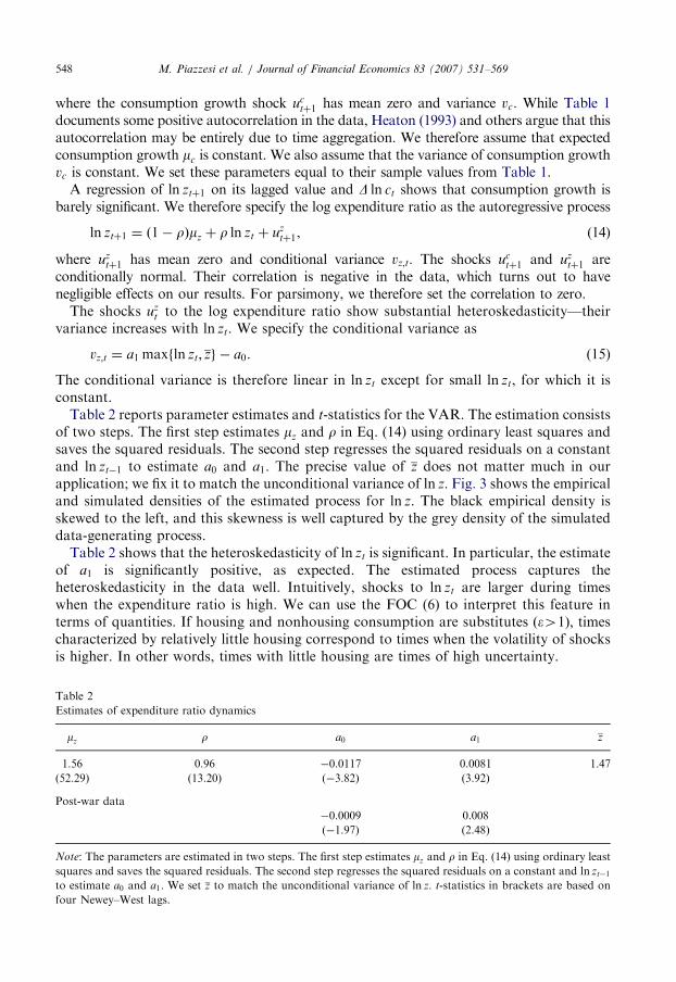
The conditional variance is therefore linear in ln zt except for small ln zt, for which it isconstant.Table 2 reports parameter estimates and t-statistics for the VAR. The estimation consists

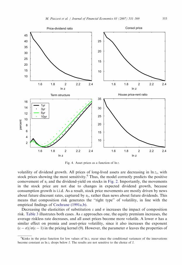
of two steps. The first step estimates mz and r in Eq. (14) using ordinary least squares andsaves the squared residuals. The second step regresses the squared residuals on a constantand ln zt�1 to estimate a0 and a1: The precise value of z does not matter much in ourapplication; we fix it to match the unconditional variance of ln z: Fig. 3 shows the empiricaland simulated densities of the estimated process for ln z. The black empirical density isskewed to the left, and this skewness is well captured by the grey density of the simulateddata-generating process.Table 2 shows that the heteroskedasticity of ln zt is significant. In particular, the estimate

of a1 is significantly positive, as expected. The estimated process captures theheteroskedasticity in the data well. Intuitively, shocks to ln zt are larger during timeswhen the expenditure ratio is high. We can use the FOC (6) to interpret this feature interms of quantities. If housing and nonhousing consumption are substitutes ð�41Þ; timescharacterized by relatively little housing correspond to times when the volatility of shocksis higher. In other words, times with little housing are times of high uncertainty.

Table 2

Estimates of expenditure ratio dynamics

mz r a0 a1 z

1.56 0.96 �0.0117 0.0081 1.47

(52.29) (13.20) (�3.82) (3.92)

Post-war data

�0.0009 0.008

(�1.97) (2.48)

Note: The parameters are estimated in two steps. The first step estimates mz and r in Eq. (14) using ordinary least

squares and saves the squared residuals. The second step regresses the squared residuals on a constant and ln zt�1

to estimate a0 and a1: We set z to match the unconditional variance of ln z: t-statistics in brackets are based on

four Newey–West lags.

ARTICLE IN PRESS

1.4 1.5 1.6 1.7 1.8 1.9 2 2.1 2.20

0.1

0.2

0.3

0.4

0.5

0.6

0.7

0.8

0.9

1

ln z

Fig. 3. Empirical density of the log expenditure ratio ln z (black line) and simulated density (gray line).


5.1.2. Long-lived assets

To price equity, we specify dividends as

D ln dtþ1 ¼ kD ln ctþ1 þ udtþ1, (16)

where k is a constant and udtþ1 is i.i.d. normal with zero mean and variance vd , independent

of all other shocks. Our results are based on k ¼ 1 and a variance vd that matches thevariance of dividend growth. The advantage of this specification is that we can allowdividend growth to be more volatile than consumption growth, and we can also allowfor an imperfect correlation between consumption growth and dividend growth. FromTable 1, we have vd ¼ 8:282 � 1:882 percent for the long sample and vd ¼ 5:262 � 1:462

percent for the post-war sample. For the long sample, this approach matches the empiricalcorrelation between consumption and dividend growth exactly, while it somewhatoverstates the correlation in the post-war sample. Below we discuss the implications ofalternative specifications.

We obtain a difference equation for the price–dividend ratio by plugging the discountfactor (9) into the pricing equation. For housing, we calculate an analogous price–dividendratio by equating the value of the housing stock with the present discounted value of allfuture housing services, qtst ¼ ct expð� ln ztÞ:

ust ¼ Et½Mtþ1ðus

tþ1 þ 1ÞekD ln ctþ1þudtþ1 �

uht ¼ Et½Mtþ1ðuh

tþ1 þ 1ÞeD ln ctþ1�D ln ztþ1 �. ð17Þ

Conveniently, the solution ust reduces to the price of a consol bond if k ¼ 0 and vd ¼ 0.

The dividend processes of all the assets we want to price can be written as functions ofthe forcing process ðD ln ctþ1; ln ztÞ plus i.i.d. shocks. Given parameters � and s and theestimated distribution of the forcing process, we determine asset prices as stationarysolutions to the stochastic difference equation (17). Although we do not specify an


exogenous endowment process explicitly, the resulting prices are equilibrium prices for aneconomy summarized by a tuple fb;s; �;o; ðc̄t; s̄tÞg, as in Section 3 Indeed, theintratemporal FOC must hold in any equilibrium of such an economy. We can thereforedefine a jointly stationary and Markov process ðD ln ct; lnðct=stÞÞ by (6) for some positivescalar o.5 An endowment process ðc̄t; s̄tÞ can then be constructed by fixing a time-zero levelof consumption, c0.The pricing kernel for the economy defined above takes the form of (9), and by

construction its distribution is the same as that of the expenditure share-based kernel weuse in our empirical work. Dividends on our assets can also be expressed in terms ofðD ln c̄tþ1; lnðc̄t=s̄tÞÞ by (6). Moreover, the Markov structure implies that their price–dividend ratios at time t depend only on ðD ln ct; lnðct=stÞÞ, as well as on the parametersðb;s; �;oÞ that enter the pricing kernel (9). In other words, the price–dividend ratios in theconstructed economy follow the same stochastic difference equation (17) that we use tocompute prices below.

5.1.3. Preference parameters

For the elasticity of intertemporal substitution, we follow Hall (1988), whoestimates s to be around 0.2. Studies based on micro data find values for s that aresomewhat higher, but not by much. For example, Runkle (1991) reports an estimateof 0.45 using micro data on food consumption. Attanasio and Weber (1995) reportestimates using CEX data between [0.48,0.67]. We refer to s ¼ 0:2 as our lo risk aversion

benchmark.Estimates of the intratemporal elasticity are more difficult to obtain. The problems with

data quality in Section 4 imply that direct estimation of the intratemporal FOC (6) isproblematic. We therefore report results for a range of � values. We focus only on values of� greater than one. This choice is based on two pieces of evidence. First, this range issuggested by the existing empirical literature. For instance, Ogaki and Reinhart (1998),who estimate � with aggregate data on durable consumption, give [1:04; 1:43] as a 95percent confidence interval (see their Table 2, p. 1091). The test for unitary elasticity � ¼ 1is thus rejected. Papers in the home-production literature also estimate � to be above one:Benhabib, Rogerson, and Wright (1991) obtain � ¼ 2:5 and McGrattan, Rogerson, andWright (1997) get 1.75.Second, we estimate the cointegrating relationship implied by the intratemporal FOC (6)

between NIPA quantity and price data for housing services. The idea is that even if thesedata are mismeasured, they may still provide useful information about long-run trends.Appendix C reports the results of this exercise. The key parameter in the cointegratingrelationship is �; which we estimate to be 1.27 with a standard error of 0.16. We alsoestimate � based on Euler equations for excess returns in Section 5.6. We obtain � ¼ 1:17and 1.24, but these come with huge standard errors. Again, however, this evidence suggeststhat � is above one.

5Our approach does not identify the parameter o. This is not necessary, since the pricing kernel implies that

when expenditure data are available, there is no need to know o in order to fully characterize the asset pricing

implications of the model. Of course, this does not mean that o does not matter for asset pricing. For example, if

o is equal to zero, housing is not valued, and we are back in the one-good case. The point is that expenditure

shares already contain the information about o that is needed. For example, any nonzero amount of expenditures

on housing implies that the value of o cannot be zero.


5.2. Numerical results

Panel A of Table 3 reviews properties of the standard CCAPM. We report first andsecond moments of annual equity premia, consol premia, and the riskless rate, all inlogarithms. We consider two parameterizations, which we compare to two benchmarkversions of the housing model below. In the case of lo risk aversion, the coefficient ofrelative risk aversion is 1=s ¼ 5, and the discount factor is b ¼ 0:99. For the hi risk

aversion case, we set the coefficient of relative risk aversion to 1=s ¼ 16, and we also makethe agent more patient with b ¼ 1:24. The two cases imply roughly the same equitypremium and riskfree rate.

As is standard in the literature, aggregate consumption growth and dividend growth arei.i.d. lognormal processes of the forms given in (13) and (16) with k ¼ 1. Therefore, theriskfree rate and the price–dividend ratio are constant. Moreover, expected excess returnsare constant and therefore not predictable. Panel A of Table 3 also illustrates other familiarproblems with the CCAPM. The CCAPM predicts a high riskfree rate of almost12 percent—the riskfree rate puzzle—as well as an equity premium of less than 60 basis points,or 0.6 percent—the equity premium puzzle. In addition, the volatility of stock returnsin the model is too small—the volatility puzzle. For example, sðersÞ ¼

ffiffiffiffiffiffiffiffiffiffiffiffiffiffiffiffiffiffiffiffiffiffiffiffiffik2� vc þ vd

pis 1.6 percent when we assume that dividends equal consumption as in Mehra andPrescott (1985), so that k ¼ 1 and vd ¼ 0. In Table 3, the volatility of stock returns ishigher, 8.2 percent, because we allow for orthogonal shocks to dividend growth, vda0.

Panel B of Table 3 reports the same financial moments for the model with housing,together with first and second moments of annual housing returns. We compute the modelfor candidate values of the intratemporal substitution � above one. In particular, Panel Bemphasizes two benchmark cases in bold-face. In the first benchmark case, hi perceived

risk, the elasticity of intratemporal substitution � is set close to the Cobb–Douglas case.Eq. (10) shows that true aggregate consumption, that is, the quantity index implied bypreferences, becomes more volatile as � approaches one. We combine � ¼ 1:05 with lo risk

aversion (1=s ¼ 5 and b ¼ 0:99). The second benchmark case has hi risk aversion

(1=s ¼ 16 and b ¼ 1:24) as well as an intertemporal elasticity of substitution � ¼ 1:25 thatis close to the point estimate (� ¼ 1:27) from Appendix C.

The two benchmark cases in Panel B deliver exactly the same mean riskfree rate andequity premium. The model generates a low and smooth riskfree rate with a mean of1.8 percent and a volatility of 0.9 percent. The equity premium is high and excess stockreturns are volatile; their mean is 3.5 percent and their volatility above 11.4 percent. Incontrast, the consol premium in the model is smaller and smoother. Its mean is 2.5 percentand its volatility is below 6.6 percent. The model also does a reasonable job with respect tohousing returns in both cases. The mean housing premium is roughly 3.7 percent with avolatility of roughly 10.1 percent.

Panel C reports properties of model-implied aggregate consumption. With hi perceived

risk, the volatility of the aggregate bundle in Eq. (10) is 9.5 percent in the long sample. Theaggregation method used by NIPA produces an aggregate bundle with lower volatility of1.6 percent (from Table 1). The higher volatility perceived by agents in our model is partlydue to autocorrelation: the agent perceives the bundle to have a first autocorrelation of60 percent, while NIPA aggregation methods result in a bundle with only 23 percentautocorrelation. Panel C also shows that with hi risk aversion, the true consumption bundlebehaves more like the NIPA bundle.


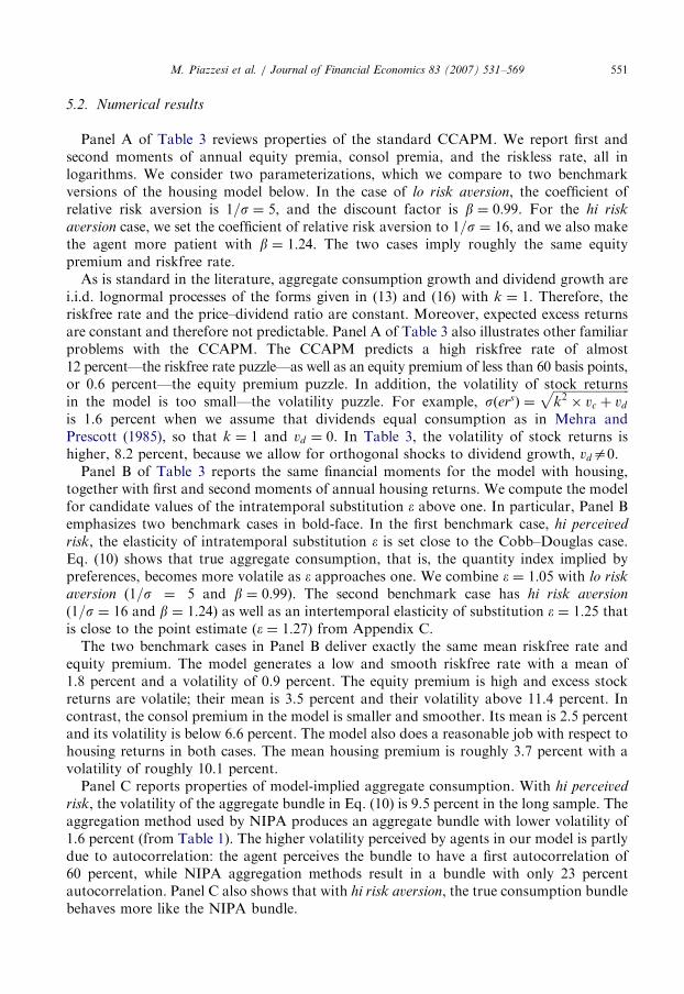
Fig. 4 plots asset prices as a function of the single state variable, the log expenditureratio ln zt. The figure, and all other figures in this paper, is based on both hi perceived risk

and Eq. (16) with k ¼ 1 and a volatility vd of orthogonal dividend shocks that matches the

Table 3

Model-implied moments of returns (%)

1=s b � Eðrf Þ EðersÞ EðerbÞ EðerhÞ sðrf Þ sðersÞ sðerbÞ sðerhÞ

Panel A. Standard CCAPM

5 0.99 11.9 0.1 0.0 0.0 8.2 0.0

16 1.24 11.1 0.6 0.0 0.0 8.2 0.0

Panel B. Housing-CCAPM

Homoskedastic shocks: vz;t ¼ constant

5 0.99 1.05 2.2 6.5 5.7 7.6 5.0 18.9 14.9 19.9

16 1.24 1.25 2.2 5.3 4.5 6.3 4.1 17.9 14.0 18.5

Heteroskedastic shocks: vz;t ¼ a1 maxfln zt; z̄g � a05 0.99 1.25 11.1 1.0 0.3 0.8 0.7 8.6 2.0 5.0

1.10 9.0 1.4 0.8 1.5 0.9 9.1 3.4 6.8

1.05 1.8 3.5 2.5 3.7 0.9 11.4 5.9 10.1

1.04 �2.3 6.0 4.4 5.6 1.8 14.9 9.1 13.6

3 1.05 5.2 1.8 1.1 1.6 0.9 10.4 5.3 9.0

4 4.2 2.5 1.7 2.7 0.6 10.7 5.5 9.7

6 �1.9 5.7 4.1 5.6 2.2 13.8 4.1 12.5

7 �4.1 9.8 5.1 6.2 3.7 18.8 10.1 13.8

16 0.99 1.25 25.5 1.1 0.1 2.4 0.5 8.4 0.1 4.5

1.24 1.25 1.8 3.5 2.5 3.9 0.5 11.9 6.6 10.5

Post-war results

5 0.99 1.05 7.5 3.0 2.7 3.1 7.5 17.0 15.2 16.7

1.05 1.0 3.7 3.2 3.8 7.5 21.4 19.4 20.9

16 1.24 1.25 2.9 2.9 2.4 3.1 6.4 17.3 15.6 16.8

1.26 1.8 3.1 2.4 3.1 6.4 18.1 16.4 17.6

Panel C. Properties of aggregate bundle for various � values

Long sample Post-war sample

� 1.04 1.05 1.10 1.25 1.04 1.05 1.10 1.25

mðD lnCÞ 2.0 2.0 2.1 2.1 4.4 3.9 3.0 2.4

rðD lnCÞ 0.59 0.60 0.62 0.56 0.62 0.62 0.62 0.56

sðD lnCÞ 12.0 9.5 4.7 2.2 9.0 7.2 3.7 1.8

Note: This table reports model-implied moments of financial returns for various assets. The financial returns are

the riskfree rate, rf , and real returns in excess of the riskfree rate on stocks, ers, long bonds, erb, and housing, erh.

The moments are mean, E, and standard deviation, s. The underlying model in Panel A is the CCAPM evaluated

at various values for the intertemporal elasticity, s, and the discount factor, b. The underlying model in Panel B is

the Housing CCAPM, which also features the intratemporal elasticity �. The main difference in the calibration of

these models is that Eq. (13) is matched to NIPA data on nondurables and services for the CCAPM, while the

calibration of the Housing CCAPM excludes housing services from Eq. (13) and specifies a process, Eq. (14), for

the log nonhousing expenditure ratio. For the case of ‘‘homoskedastic shocks’’ to this process, a1 ¼ 0 in Eq. (15),

and the parameter a0 is estimated as variance of the residuals in Eq. (14). For the case of ‘‘heteroskedastic

shocks’’, we use the a0 and a1 estimates from Table 2. Panel C reports the mean, m, autocorrelation, r, andstandard deviation, s, of the growth rate of aggregate consumption, D lnC, defined in Eq. (10) for various values

of �.

ARTICLE IN PRESS

1.6 1.8 2 2.2 2.4

10

15

20

25

30

35

40

45

Price-dividend ratio

ln z

1.6 1.8 2 2.2 2.4

10

15

20

25

Consol price

ln z

1.6 1.8 2 2.2 2.4

2

4

6

8

10

12

14

16

ln z

perc

ent

Term structure

1yr

3yr

5yr

10yr

1.6 1.8 2 2.2 2.4

10

15

20

25

30

35

House price-rent ratio

ln z

Fig. 4. Asset prices as a function of ln z.


volatility of dividend growth. All prices of long-lived assets are decreasing in ln zt; withstock prices showing the most sensitivity.6 Thus, the model correctly predicts the positivecomovement of at and the dividend-yield on stocks in Fig. 2. Importantly, the movementsin the stock price are not due to changes in expected dividend growth, becauseconsumption growth is i.i.d. As a result, stock price movements are mostly driven by newsabout future discount rates, captured by at, rather than news about future dividends. Thismeans that composition risk generates the ‘‘right type’’ of volatility, in line with theempirical findings of Cochrane (1991a,b).

Decreasing the elasticities of substitution � and s increases the impact of compositionrisk. Table 3 illustrates both cases. As � approaches one, the equity premium increases, theaverage riskless rate decreases, and all asset prices become more volatile. A lower s has asimilar effect on premia and asset-price volatility, since it also increases the exponentð�� sÞ=sð�� 1Þ in the pricing kernel (9). However, the parameter s leaves the properties of

6Kinks in the price function for low values of ln zt occur since the conditional variances of the innovations

become constant as ln zt drops below z̄. The results are not sensitive to the choice of z̄.


the aggregate bundle and its price index unchanged. Lowering s therefore has thestandard effect of increasing the riskless rate since agents who like to substituteconsumption push the riskless rate up in a growing economy. To keep the riskfree ratelow, we need to make the agent more patient. This can be accomplished with a higherdiscount factor, b.

5.3. Volatility and premia

Our numerical results are based on the nonlinear pricing kernel (9). To gain intuitionabout the unconditional moments reported in Table 3, it is helpful to linearly approximatethe log kernel. Writing Mtþ1 ¼ be�ð1=sÞD ln ctþ1þ½ð��sÞ=sð��1Þ�D ln atþ1 and linearizing D ln atþ1

around the point ztþ1 ¼ zt, we obtain7

Mtþ1 � b exp �1

sD ln ctþ1 þ

ð�� sÞsð�� 1Þ

ð1� atÞD ln ztþ1

� �. (18)

5.3.1. Riskfree rate

Conditional normality of ðD ln ct; ln ztÞ and approximation (18) also lead to a convenientformula for the riskless interest rate:

rftþ1 � � ln bþ

1

smc �

1

2s2vc

þ ð1� atÞ �ð�� sÞsð�� 1Þ

ð1� rÞðmz � ln ztÞ �1

2

�� ssð�� 1Þ

� �2ð1� atÞvz;t

( ). ð19Þ

The effect of consumption risk on the riskfree rate is familiar and is captured by the firstline of the equation. If consumption is expected to grow, agents try to borrow, pushing theinterest rate up. If consumption growth becomes more uncertain, agents try to engage inprecautionary saving, pushing the interest rate down. Both effects are stronger the moreagents want to smooth consumption (low s). Since consumption is not very volatile, theprecautionary savings effect is small for reasonable values of s; this is the riskfree ratepuzzle. Also, consumption risk does not lead to time variation in interest rates, becauseconsumption growth is not forecastable and its variance is constant over time.The effect of composition risk on the interest rate is represented by the expression in

braces. The presence of composition risk implies that, on average, the riskfree rate is lower.This is because agents worry about composition risk and therefore attempt to save moreon average. Formally, suppose the expenditure ratio ln zt is equal to its unconditionalmean mz. The first term in braces then collapses to zero, while the second term is negative,since at is always smaller than one. Precautionary savings induced by the volatility vz;t ofshocks to the expenditure ratio therefore pushes the riskfree rate down. Thus, compositionrisk helps resolve the riskfree rate puzzle.

7The approximation is not exact. In particular, it masks the fact that in the nonlinear kernel, the correlation

with consumption growth will be also be weighted differently as at changes. This effect will be made explicit by

picking a different linearization point. For example, one could assume an AR(1) process for ln zt and linearize

around the conditional mean. The current approximation is simpler and is sufficient to interpret the

computational results, which are based on the true nonlinear kernel.


Composition risk also leads to variation in the riskless rate. There are two effects atwork. First, there is a new intertemporal substitution effect. Agents try to borrow in severerecessions, when the expenditure ratio ln zt is high and housing consumption is relativelylow. In severe recessions, agents correctly expect that better times are ahead, because theexpenditure ratio will revert to its mean. In Eq. (19), the intertemporal substitution effect iscaptured by the first term in braces: the interest rate increases when ln zt is higher than itsunconditional mean mz.

The second effect is that the strength of the precautionary savings motive varies overtime with the amount of composition risk. Agents worry more about composition risk insevere recessions, when shocks to the expenditure ratio are larger. Indeed, by (15), anincrease in ln zt goes along with an increase in the conditional variance vz;t and therebyincreases the second term in braces. As a result, agents try to save more in severe recessionsand therefore push the interest rate down. The precautionary savings effect thuscounteracts the intertemporal substitution effect and reduces the volatility of the risklessrate.8

At the same time, heteroskedasticity does not fully neutralize the intertemporalsubstitution effect. This is because the impact of heteroskedasticity is diminished as thenonhousing share rises: the second term is multiplied by ð1� atÞ. Indeed, as at approachesone, the precautionary savings effect will vanish faster than the intertemporal substitutioneffect. This implies that the interest rate for high at will be higher than its mean. At least forhigh at, we can therefore expect an interest rate function that is increasing in at. Figs. 3 and4 confirm the intuition that the riskless rate is very stable in the part of state space that hashighest probability. Indeed, it is non-monotonic in this area, as a result of thecounteracting precautionary savings and intertemporal smoothing effects.

5.3.2. Risk premia

The expected return ri on an asset in excess of the riskless rate is now approximately

Etðritþ1Þ � r

ftþ1 þ

1

2vartðr

itþ1Þ �

1

scovtðD ln ctþ1; r

itþ1Þ

� ð1� atÞð�� sÞsð�� 1Þ

covtðD ln ztþ1; ritþ1Þ. ð20Þ

The risk premium on any asset depends on the conditional covariance of its return withtwo factors, nonhousing consumption growth and the change in the expenditure ratio. Theconditional covariance of returns and nonhousing consumption growth is small. However,Fig. 4 shows that the prices of long-lived assets such as stocks and consols move oppositeto the composition risk factor ln zt, so that returns are negatively correlated with D ln zt. Inlight of the second term on the right hand side of (20), this is exactly what is needed togenerate additional premia due to composition risk. In addition, leverage and growth individends implies that stock prices are more volatile than consol prices. As a result, theequity premium is larger and more volatile than the consol premium.

The model also implies that expected excess returns vary over time. This is illustratedin Fig. 5, which plots the model-implied dividend yield and expected returns over the

8As we mention in Section 2, Campbell and Cochrane (1999) also rely on heteroskedasticity. However, their

estimates of the heteroskedasticity parameters are based on moments of asset prices—the volatility of the riskfree

rate. Our estimates from Table 2 are only based on macroeconomic data.

ARTICLE IN PRESS

1940 1950 1960 1970 1980 1990 2000

2

4

6

8

10 Expected excess stock return

Riskless rate

Dividend yield

Per

cent

Per

cent

1940 1950 1960 1970 1980 1990 2000

3

4

5

6

Fig. 5. Model-implied expected excess returns and dividend yield.

M. Piazzesi et al. / Journal of Financial Economics 83 (2007) 531–569556

post-war period. It is apparent that the dividend yield is a slow-moving state variable thatforecasts returns. This is consistent with recent empirical evidence, which we comparemore closely with the model’s implications in Section 5.4. Moreover, the model predictsthat at, which is highly correlated with the dividend yield, should also be a goodforecasting variable. This is indeed the case in the data, as we document in Section 5.5.

5.3.3. Price volatility of long-lived assets

To understand the role of discount rate news for prices, it is useful to first abstract fromheteroskedasticity. We can then use (18) to define a state-dependent discount rate dtþ1 ¼

� lnMtþ1 and rewrite the price–dividend ratio (17) as

usðln ztÞ ¼ Et½e�ðdtþ1þkD ln ctþ1þud

tþ1Þð1þ usðln ztþ1ÞÞ�

¼ Et

X1j¼1

exp �Xj

i¼1

dtþi

!exp

Xj

i¼1

kD ln ctþi þ udtþi

!" #

¼X1j¼1

bjeððk�1=sÞmcþ12ðk�1=sÞ

2vcþ12vd ÞjEt exp �

ð�� sÞsð�� 1Þ

Xj

i¼1

ð1� atþiÞD ln ztþi

!" #

¼X1j¼1

u�j ðkÞwjðln ztÞ.


Here, u�j ðkÞ is the present discounted value, adjusted for consumption risk and normalizedby current dividends, of a claim to dividends in period tþ j. In other words, it is the priceof such a claim in the standard CCAPM divided by current dividends. With i.i.d.consumption, this ratio is constant, which amounts to a version of the volatility puzzle. Inour Housing CCAPM, volatility is induced by the new discount factor for composition riskwjðln ztÞ. Innovations to ln zt provide news about current and future discount rates dtþj. Inline with the empirical findings of Cochrane (1991a,b), it is this type of news, not newsabout dividends, that accounts for most changes in prices.

The above formula also clarifies the relationship between stock and consol prices. On theone hand, as long as u�j is increasing in k, the price–dividend ratio is larger and morevolatile than the consol price. The random factor wjðln ztÞ affects consols and stocks in thesame way; differences across assets exist only to the extent that there are differences inu�j ðkÞ. The latter is increasing if mc4

12ð1=s� kÞvc þ

12

vd=ð1=s� kÞ. An increase in k

increases both mean growth and dividend risk. If risk aversion and consumption risk arenot too high, the mean effect dominates and the price–dividend ratio goes up. On the otherhand, mean reversion in the nonhousing ratio ln zt implies that both prices move oppositeto ln zt. Unfortunately, the discount factor wjðln ztÞ is not available in closed form, since zt

itself is a nonlinear function of at. However, numerical results for the homoskedastic case(not shown) deliver a shape much like Fig. 4. If ln zt is large, then D ln ztþ1 is negative withhigh probability, that is, housing expenditure is expected to grow faster than numeraireexpenditure. This makes saving in numeraire terms relatively less attractive and hencelowers asset prices.

In the case of heteroskedasticity, bad times are associated with more composition risk.This is captured by the fact that vz;t goes up with ln zt, which has two effects. First, itdampens the response of prices to a unit change in the log expenditure ratio ln zt. Thereason is that an increase in risk encourages precautionary savings, so that agents discountthe future less. Therefore, prices fall by less than in the homoskedastic case. Second, thesize of the typical shock is larger when ln zt is high. This tends to increase the conditionalvolatility of returns when ln zt is high. On net, the variance of returns and their associatedpremia therefore tend to be higher in the heteroskedastic case.

Fig. 4 also shows that our measure of the value-rent ratio for the housing stock respondsmuch less to a change in zt than the price–dividend ratio. The reason is that while anincrease in ln zt increases discount rates, it also increases the expected growth rate ofhousing dividends, D ln ctþ1 � D ln ztþ1: Since the nonhousing ratio reverts to its mean, ahigh value today predicts an increase in housing expenditure in the future. This increasesthe current value of the housing stock, partly offsetting the increase in discount rates. Inour model, houses are therefore less risky than stocks and hence they command a lowerpremium.9 The price dynamics also suggests the share of housing in total wealth,ctztus

t=ðctust þ ctztus

tÞ ¼ ð1� atÞuht =ðv

ht þ vs

tÞ, as another candidate variable for forecastingreturns. We do not pursue this implication in the current paper, since it would require dataon wealth.

9Housing returns computed from the model according to Eq. (17) not only measure the returns on one unit of

housing, but also include the value of new housing. Housing returns computed for Table 1 do not include the

value of new housing. When we do include the value of new housing, mean returns go up by 2.5 percentage points.

The standard deviation of housing returns is unchanged.


5.3.4. Post-war performance

To see how the model behaves over the post-war sample, we report results for the twobenchmark parameterizations in the last four rows of Panel B in Table 3. Composition riskstill leads to substantial average excess returns on stocks. The model also still generateshigh volatility of stock returns. However, a larger portion of these effects is nowattributable simply to a term premium—compensation for holding a long-maturity asset—as opposed to an equity premium. The reason is that the model generates more volatility inthe riskfree rate when we calibrate to post-war data, and term premia increase tocompensate for this higher volatility.To understand the increase in sðrf Þ; consider the parameter estimates in Table 2. Over

the long sample, the estimates show substantial time variation in the volatility of theexpenditure share at. In particular, the volatility of at increases during bad times, when theexpenditure share at is high. This higher risk generates a motive for precautionary savings,which pushes the riskfree rate down. In the shorter post-war sample, there is still evidenceof heteroskedasticity in the expenditure share at. Table 2 shows that the parameter a1;which governs the dependence of the conditional variance on ln zt, is still estimated to besignificant. The point estimate of a1; however, is much smaller than the long-sampleestimate. When we calibrate the model to post-war data, agents thus have less reason tosave in bad times, which increases the risk-free rate during bad times relative to good times.This time variation in the risk-free rate leads to higher volatilities sðrf Þ of around 7 percentin Panel B.Another, albeit less important, difference between the model implications over the two

samples is that the mean of the riskfree rate is lower over the long sample. The reason isthat there were large shocks to the expenditure share in the first half of this century,increasing our point estimate of the unconditional volatility of the expenditure sharerelative to that of the post-war experience. This higher average composition risk leads tomore precautionary savings, and thus a lower risk-free rate on average. Comparing ourbenchmark results in Panel B to the post-war results reveals the effect of this decrease inunconditional volatility on Eðrf Þ. This effect can be easily counteracted, however, byincreasing the discount factor b to values above one. The results with hi perceived risk showthat the model still generates a low average short rate for b ¼ 1:05, while the same is truefor b ¼ 1:26 with hi risk aversion.

5.3.5. Alternative dividend specifications

To investigate how the specification of dividends in Eq. (16) affects our results, weconsider the following three cases:

a.
dividends are equal to consumption plus i.i.d. shocks, k ¼ 1, and vd40. The parametervd is selected to match the volatility of dividend growth.
b.
dividends are equal to consumption, k ¼ 1, and vd ¼ 0. c. dividends are equal to a levered-up version of consumption, k41, and vd ¼ 0. The
constant k is selected to match the volatility of dividend growth.

The results in all our tables are based on case a, which is arguably the most realisticspecification since it captures both the relative volatility and the correlation betweenconsumption growth and dividend growth. We now report some results for cases b and cbecause they frequently appear in the literature. Case b is the specification of Mehra and


Prescott (1985). Case c, due to Campbell (1986) and Abel (1999), captures the fact thatdividend growth is more volatile than consumption growth, but assumes that the two areperfectly correlated. At our parameter values, Table 1 implies that k ¼ 8:28=1:88 ¼ 4:4 forthe long sample and k ¼ 5:26=1:46 ¼ 3:6 for the post-war sample.

We find that the specification of dividends matters for the size of the equity premiumand the volatility of equity returns implied by the model. Specifically, cases a and b implyroughly the same equity premium: the short rate is unaffected by the specification ofdividends and average stock returns in c are only slightly lower.10 However, equity premiain case c are more than twice as large as the numbers reported in Table 3. Intuitively, theagent does not worry about shocks to dividends ud that are orthogonal to consumption:since these shocks do not represent systematic risk, they do not increase the equitypremium. The amount of systematic risk in dividend growth is roughly the same in cases aand b, because k ¼ 1 in both specifications. In contrast, the amount of systematic risk incase b is much higher, because the entire volatility of dividend growth is due to shocksthat are perfectly correlated with consumption growth, and so the equity premium ishigher. Of course, any shocks to dividend growth, whether systematic or not, increase thevolatility of stock returns, so the volatility of stock returns in cases a and c is much higherthan in case b.

5.4. Predicting excess returns with the dividend yield

The model implies that excess returns are predictable. In particular, excess returns onstocks can be predicted from the dividend yield. This can be seen in Fig. 4, which showsthat the dividend yield is a function of the stationary variable ln zt: The dividend yieldinherits the persistence and mean reversion from ln zt: If the dividend yield is high, itpredicts a lower dividend yield and thus a higher price–dividend ratio in the future.Together with i.i.d. dividend growth and a smooth riskfree rate, a high dividend yieldtherefore predicts high excess returns. Intuitively, expected excess returns are higher insevere recessions (times when ln zt is high), because investors demand higher compensationfor composition risk in those times.

To determine how much predictability the model generates, we simulate 50,000 samplepaths at the two sets of benchmark preference parameters. For each simulated path, weregress excess returns on a constant and the dividend yield. We also run the sameregression with historical data. The ‘‘Model’’ columns in Table 4 report average slopecoefficients and average R2s based on the simulated data with hi perceived risk and hi risk

aversion, respectively. The results indicate that the slope coefficient is positive andincreasing, as we vary the forecasting horizon from one to five years. The R2s also increasewith the forecasting horizon. The ‘‘Long sample’’ and ‘‘Post-war sample’’ columns reportthe corresponding results based on historical data. The model-implied regressioncoefficients are between 0.14 and 0.60. The empirical regression coefficients arecomparable, between 0.11 and 0.52. The model also does a good job in matching the

10To see why, it is useful to consider a solution ustþ1 to the difference equation (17) without dividend shocks,

vd ¼ 0. The price–dividend ratio with shocks, vda0, is larger, because it solves the same equation, but with a

higher discount factor. Since the logarithm is concave, the mean of ln ðustþ1 þ 1Þ � ln ðus

tÞ is lower and thus average

stock returns are lower. However, the difference between cases a and b is small, always lower than 30 basis points,

or .3 percentage points, for the models considered in the various rows of Table 3.

ARTICLE IN PRESS

Table 4

Predicting excess returns with the dividend yield

Horizon Hi perceived risk model Hi risk aversion model Long sample Post-war sample

(yr) Slope R2 Slope R2 Slope t-stat R2 Slope t-stat R2

1 0.15 0.05 0.14 0.06 0.11 2.51 0.07 0.11 2.25 0.08

2 0.29 0.09 0.27 0.10 0.21 2.15 0.12 0.21 1.95 0.12

3 0.41 0.13 0.39 0.15 0.24 1.70 0.11 0.24 1.53 0.11

4 0.51 0.16 0.50 0.18 0.32 1.63 0.13 0.32 1.41 0.11

5 0.60 0.19 0.59 0.21 0.49 2.49 0.19 0.52 2.26 0.17

Note: We report regression results of log excess stock returnsPn

j¼1rstþj � r

ftþj on a constant and the log dividend

yield ln 1=vst for n ¼ 1; . . . ; 5 years. The ‘‘Model’’ columns contain the average slope and R2 over 50,000 simulated

samples with 65 observations. The model with hi perceived risk is the bold-face parameterization in Table 3 with

� ¼ 1:05, b ¼ 0:99, and 1=s ¼ 5. The model with hi risk aversion is the bold-face parameterization in Table 3 with

� ¼ 1:25, b ¼ 1:24, and 1=s ¼ 16. The ‘‘Long sample’’ columns run regressions with 1936–2001 historical data,

and the ‘‘Post-war sample’’ columns use 1947–2001 data. t-statistics are based on Newey–West standard errors to

correct for overlapping observations.


R2s; the model-implied R2s are within two to four percentage points of their empiricalcounterparts.

5.5. Predicting excess returns with expenditure

Interestingly, the model also implies that a macroeconomic variable, the expenditureshare at, should be a good forecasting variable. Intuitively, the model implies that at is highin severe recessions, when expected excess returns are high. To investigate this implicationof the model, we again simulate 50,000 samples from the model at the two sets ofbenchmark preference parameters. For each simulated sample path, we regress log excessstock returns on a constant and the log expenditure share ln at. The ‘‘Model’’ columns inPanel A of Table 5 report the average slope coefficient and the average R2 from theseregressions. The results indicate that the expenditure share predicts excess returns with apositive sign. The slope coefficient increases from 2.0 to 9.3 as the forecasting horizonincreases from one to five years. The 5–21 percent R2s are comparable to the 5–21 percentR2s in Table 4 based on the dividend yield, and they also rise with the horizon.The ‘‘Long sample’’ columns run the corresponding regression results with historical

data over the whole sample, while the ‘‘Post-war sample’’ results use the post-war period.We can see that both the 1.6–10.7 slope estimates and the 2 to 22 percent R2 arecomparable to those in the model. Panel B of Table 5 reports the results from regressinghistorical excess returns on both the expenditure share and the dividend yield. The resultsindicate that the expenditure share outperforms the log dividend yield, especially overlonger forecasting horizons. The t-statistics of the expenditure share coefficient are larger,while the slope coefficients and R2s from the univariate regression in Panel A remainalmost identical. Like many macroeconomic models, returns in our setup are driven byonly a few shocks. This implies that the two variables are highly correlated, and thus itdoes not make sense to run this horse race in the simulated data.Predictability of excess returns, both in our model and in the data, crucially depends on

whether the price–dividend ratio is stationary. In our model, price–dividend ratios inherit

ARTICLE IN PRESS

Table 5

Predicting excess stock returns with the expenditure share

Horizon Hi perceived risk model Hi risk aversion model Long sample Post-war sample

(yr) Slope R2 Slope R2 Slope t-stat R2 Slope t-stat R2

Panel A. Regressions on expenditure share

1 2.00 0.05 2.40 0.06 1.36 1.47 0.02 1.42 1.68 0.03

2 3.80 0.09 4.55 0.10 3.30 2.03 0.07 3.68 2.24 0.08

3 5.42 0.13 6.50 0.14 5.01 2.40 0.14 6.25 3.21 0.20

4 6.88 0.16 8.25 0.18 6.58 2.84 0.18 8.63 3.95 0.28

5 8.19 0.19 9.83 0.21 8.44 3.65 0.22 10.73 4.92 0.30

Long sample Post-war sample

Horizon ln 1=vst ln at ln 1=vs

t ln at

(yr) Slope t-stat Slope t-stat R2 Slope t-stat Slope t-stat R2

Panel B. Regression on expenditure share and dividend yield

1 0.10 2.04 0.43 0.44 0.07 0.10 1.84 0.50 0.13 0.08

2 0.17 1.60 1.75 1.11 0.14 0.16 1.39 2.14 0.75 0.14

3 0.15 1.01 3.65 1.77 0.18 0.10 0.66 5.30 2.11 0.21

4 0.16 0.86 5.08 2.29 0.20 0.06 0.30 8.09 3.04 0.28

5 0.28 1.49 5.87 2.64 0.26 0.15 0.81 9.24 3.43 0.31

Note: Panel A reports regression results of log excess stock returnsPn

j¼1rstþj � r

ftþj on a constant and the log

expenditure share ln at for n ¼ 1; . . . ; 5 years. The ‘‘Model’’ columns contain the average slope and R2 over 50,000

simulated samples with 65 observations. The model with hi perceived risk is the bold-face parameterization in

Table 3 with � ¼ 1:05, b ¼ 0:99, and 1=s ¼ 5. The model with hi risk aversion is the bold-face parameterization in

Table 3 with � ¼ 1:25, b ¼ 1:24, and 1=s ¼ 16. The ‘‘Long sample’’ columns run regressions with 1936–2001

historical data, and the ‘‘Post-war sample’’ columns use 1947–2001 data. t-statistics are based on Newey–West

standard errors to correct for overlapping observations. Panel B reports regression results ofPn

j¼1rstþj � r

ftþj on a

constant, ln at; and the log dividend yield ln 1=vst :


the persistence properties of the log expenditure ratio ln zt. From Table 1, we know thatln zt is highly persistent; its autocorrelation is 0.964 estimated over the long sample and0.83 over the post-war sample. In what follows, we discuss theoretical and statisticalreasons to believe that the log expenditure ratio is stationary, and evidence that suggeststhat the predictability results in Table 5 do not suffer from small-sample bias.

To see the theoretical reasons, consider a model in which ln zt is a random walk. In thissetup, the probability that the process ln zt will stay within some finite range ½ln z; ln z�

forever is zero. This implies that the probability that the expenditure share at will staywithin the finite range ½a; a� with a ¼ z =ð1þ zÞ and a ¼ z=ð1þ zÞ is zero as well.Economically, this means that expenditures on housing will either become negligible ordominant over time—both cases are implausible. Even in finite samples, the random-walkspecification implies that there is a high probability of observing at values outside the rangeof values A ¼ ½0:81; 0:87� observed historically. For example, simulations show thatPrðateA for some tp100Þ ¼ 90 percent if we assume that ln zt is a random walk.

To investigate the statistical evidence for stationarity, we test for a unit root byconducting a series of augmented Dickey–Fuller (ADF) tests. We use Schwarz and Akaikecriteria to select the maximum lag length k of lagged difference terms in the ADF testequation. For the full sample, k equals one and nine, respectively, and we reject the null of


a unit root even at the 1 percent level. Of course, the evidence against a unit root is weakerin the post-war sample. We are not able to reject the null at conventional test sizes in thisshorter sample.The persistence of the expenditure share raises the concern that the predictability

regressions in Table 5 give biased results in small samples. Stambaugh (1999) derives aformula for the bias for the slope coefficient in univariate regressions. The formulaexpresses the bias as some multiple b times the small-sample bias in the autoregressivecoefficient of the right-hand side variable, which is typically negative. The multiple b is theratio of the covariance of the innovations of right-hand side and left-hand side variablesdivided by the RHS innovation variance.11 For the log expenditure share used in Table 5,we estimate b to be equal to �2:0, �1:3, �0:1, �2:9, and 5:2 estimated over the long sampleat the one-, two-, three-, four- and five-year horizon, respectively.This suggests that the bias is small. For example, at the one-year horizon, we estimate

the autoregressive coefficient of ln at to be 0.96. The downward bias in this estimate is atmost 0.04. Therefore, the bias in the slope coefficient is below 0.08, which is small relativeto the slope coefficient of 1.36 in Table 5. Similar results obtain for the other horizons; infact, the positive b estimate for the five-year horizon even biases against findingpredictability. Intuitively, the reason for this finding is that, unlike the dividend yield andother commonly used predictor variables, the expenditure share is a macroeconomicvariable and thus covaries less with returns. This lower covariance helps avoid small-sample bias.As an alternative check, we run the predictability regressions with nonoverlapping data.

To be precise, we run log excess stock returnsPn

j¼1rstþj � r

ftþj on a constant and the log

expenditure share ln at for t ¼ 1; 1þ n; 1þ 2n; . . . and n ¼ 1; . . . ; 5 years. The resultingslope coefficient estimates are 1.4, 1.8, 5.4, 8.0, and 7.6 with t-statistics of 1.5, 1.2, 2.8, 3.9and 3.7. Although concern about small-sample bias remains, these different pieces ofevidence show that the results in Table 5 are not obviously biased.

5.6. GMM based on Euler equations

We thus far solve for returns implied by the model at a range of values for the preferenceparameter �. It is also possible to estimate � from Euler equations based on returns data.We consider unconditional Euler equations E½ðRi

tþ1 � Rftþ1ÞMtþ1� ¼ 0 based on the pricing

kernel (9). We fix the coefficient of relative risk aversion at 1=s ¼ 5 and estimate � using thegeneralized method of moments (GMM) with excess stock returns (i ¼ s). This approachreflects our prior that risk aversion should be low. (The value for the discount factor b doesnot matter for excess returns.) The resulting estimate for � is 1.17 and its 95 percentconfidence interval is ½1:014;1Þ. To compute this confidence interval, we use the fact thatthe GMM objective function JT multiplied by the number of observations T is distributedw2 under the null hypothesis. Specifically, we evaluate the GMM objective function JT ð�Þfor different values of � and determine the parameter region for which T � JT ð�Þ is smaller

11To be precise, Stambaugh (1999) considers the regressions: yt ¼ aþ bxt�1 þ ut and xt ¼ yþ rxt�1 þ vt.

Stambaugh’s Proposition 4 derives the following expression for the small sample bias: E½b̂� b� ¼ b� E½r̂� r�,where b ¼ covðut; vtÞ=varðvtÞ. To compute the bias for longer horizons n, we take the errors ut and vt from the

regression equations yt ¼ aþ bxt�n þ ut and xt ¼ yþ rxt�n þ vt estimated with data sampled at dates

1; 1þ n; 1þ 2n; . . ., so that there is no overlap.


than its 5 percent critical value. The usual GMM standard errors turn out to be huge,independent of the number of lags in the Newey–West weighting matrix.

When we add housing returns (i ¼ s; h) as a second moment, the estimate is 1.24 and its95 percent confidence interval is ½1:015;1Þ. The J-test statistic is 0.31, which is smallerthan the 5 percent w2ð1Þ critical value, 3.84, so we fail to reject the model. To summarize,the GMM estimation results are not very informative, but at least the point estimates areroughly consistent with the values we used earlier. In particular, � is above one.

6. Conclusion

We introduce an equilibrium model for asset pricing with housing. Agents care aboutthe composition of a consumption basket that contains shelter and other goods. Wecalibrate the model to data on nonhousing consumption and housing expenditures.Compared to the standard CCAPM, our model implies higher equity and housing premia,higher stock return volatility, a lower riskfree rate (which is not volatile), and lower bondpremia. It also predicts that the dividend yield and the nonhousing expenditure share at

forecast future excess stock returns. We document that the expenditure share at predictsexcess stock returns in the data better than does the dividend yield. This is particularlyinteresting because, contrary to common predictor variables, at is not based on assetmarket data.

Appendix A. Microevidence on expenditure shares

We use data from the Consumer Expenditure Survey (CEX) to obtain microevidence onexpenditure shares. Table A1 reports summary statistics of the housing expenditure shareacross different groups of households. The groups are classified by income quintile, regionof residence, age of the person who rents or owns the house, race, number of persons in thehousehold, housing tenure, and education. For renters, the data on housing expendituressimply measures rent. For homeowners, the data measures actual expenditures on shelter(such as mortgage interest and charges, maintenance, repairs, insurance, property taxesand other expenses) and do not include expenditures on household operation, house-keeping supplies, etc.

Table A1 reports average housing expenditure shares together with their standarddeviations over time (in brackets). The data are the available annual CEX series for theyears 1984–2002. Table A1 suggests that average expenditure shares across differenthousehold characteristics are very similar. For example, poorer households do not seem tospend much more on housing than do richer households. The lowest income quintilespends 17.8 percent on housing, while the highest quintile spends 16.9 percent. This findingis further supported by the fact that education levels do not seem to matter much forexpenditure shares. The households with less than a high school degree spend 18.2 percenton housing, while households with higher degrees (such as masters and doctorates) spend19.9 percent. These facts suggest that the homogeneity assumption on preferences issupported by these microdata. Another interesting finding is that older households do notseem to spend much less on housing. For example, households that are 75 years and olderspend 17.5 percent, whereas the youngest households spend 18.9 percent and 20 percent.

By and large, the differences in average expenditure shares in Table A1 seem small.Interestingly, the housing expenditure shares do not vary much over time. Most standard

ARTICLE IN PRESS

Table A1

Microevidence on expenditure shares from the CEX

Income quintiles Regions

1st 2nd 3rd 4th 5th Northeast Midwest South West

Mean 17.8 20.0 18.0 16.4 16.9 19.9 16.2 15.8 20.4

Std 1.0 1.0 1.0 0.8 0.9 1.8 1.0 0.7 0.9

Age Race

o25 25–34 35–44 45–54 55–64 65–74 75+ Hispanic Nonhisp.

Mean 18.9 20.0 18.8 16.7 15.5 15.6 17.5 20.3 18.5

Std 1.0 0.8 1.1 1.4 1.3 0.9 0.9 0.5 0.5

Number of persons Home Race

1 2 3 4 5+ Owner Renter Black Nonblack

Mean 21.6 17.1 17.0 17.3 17.2 16.4 21.8 18.9 17.7

Std 1.0 0.8 1.1 1.1 0.8 1.0 1.1 1.3 0.9

Education

I II III IV V VI VII VIII

Mean 18.2 17.7 18.2 19.9 19.9 19.9 18.1 18.5

Std 0.5 0.5 0.5 0.6 0.5 0.8 0.4 0.4

Note: Annual data, 1984–2002, from the CEX. The series of 5+ persons per households starts in 1988. The series

on hispanics/nonhispanics starts in 1994. The education series starts in 1996. The levels correspond to the

following: I ¼ less than high school, II ¼ high school graduate, III ¼ associate degree, IV ¼ college degree, V ¼

Bachelor’s degree, VI ¼Master, professional doctorate, VII ¼ less than college graduate, VIII ¼ high school with

some college.


deviations in Table A1 are below 1 percent/yr. The highest standard deviation is 1.8percent in the Northeast.12 These values are amazingly consistent with the standarddeviation of the aggregate expenditure share in Table 1.To summarize, the CEX evidence does not reveal large differences in expenditure shares

across different groups of households. For each group, the CEX evidence also suggeststhat these expenditure shares are not volatile over time. This microevidence thereforeconfirms the aggregate evidence from Section 4—preferences are different fromCobb–Douglas, but � is still close to one.

Appendix B. Data on housing returns

This appendix defines our NIPA-based measure of house prices and compares it withreturns based on alternative measures. We define housing returns according to the NIPAtables as follows. The real housing value ph

t ht is recorded in NIPA Fixed Asset Table 2.1, line68. This series computes the nominal housing value using the current value method, which

12It is tempting to interpret these standard deviations as standard errors for average expenditure shares. This is

not appropriate, however, since it ignores CEX measurement error within groups.


measures the current market value of the assets (as opposed to the historical value method,which measures the book value of assets). The series records the year-end value of residentialhousing structures. To include the value of land, we assume that land prices are perfectlycorrelated with the price of structures. Using Census data, we estimate that the value of theland is 36 percent of the total housing value. We therefore adjust houses prices toph

t =ð1� 0:36Þ. The dividends on housing are rent payments during that year, qtst: We followFlavin and Yamashita (2002) and assume that maintenance roughly equals depreciation, sothat we need to subtract dph

t�1ht�1 from dividends. We also subtract net real property taxpayments ð1� 0:33Þ � 0:025� ph

t�1ht�1, where the marginal tax rate is assumed to be 33percent and the property tax rate is assumed to be 2.5 percent. The real housing return is thus

ðpht ht þ qtstÞ=ht

ðpht�1ht�1Þ=ht�1

� d� ð1� 0:33Þ0:025. (21)

The summary statistics in Table 1 are based on this definition of returns.Davis and Heathcote (2005) use the price index for new residential investment from

NIPA Table 7.6, line 38, as their measure of house prices pht : This series is a chain-type

price index for investment in private residential structures starting in 1947, and it does alsonot include the value of land. This index mimics our index best among all the indexes; thecorrelation of price changes between this index and our house price index is 0.80.

An alternative price index is provided by the Office of Federal Housing EnterpriseOversight (OFHEO). Starting in 1975, this index tracks the changes in the value of single-family homes through repeat sales using the mortgage transaction data provided by FannieMae and Freddie Mac. The OFHEO index reflects the cost of structures and land,simultaneously controlling for the quality of the house. The series does not go back veryfar, however. The correlation of price changes with our index is 0.71 over the 25 years forwhich we have data on the OFHEO index.

The National Association of Realtors (NAR) publishes indexes that report medianhouse prices starting in the early 1960s. The Bureau of the Census also reports median andaverage sale prices of houses sold in the United States since 1963. These indexes do notcontrol for quality of the median house. The Census Bureau also publishes constant-quality price indexes that do not include the value of the land, but correct for the qualityproblem. These indexes are also available starting in the early 1960s.

Flavin and Yamashita (2002) use the Panel Study of Income Dynamics (PSID) data onhouse prices to estimate the housing returns over the 1968 to 1992 period. Unlike the otherhouse price measures we discussed above, PSID house price data is at the homeownerlevel. Returns can therefore be computed for individual houses. However, the PSIDpresent no rent data accompanying house prices. Flavin and Yamashita therefore computereal housing returns as

pht þ rf ph

t�1 þ tPropertytaxt

pht�1

¼ph

t

pht�1

þ rf þ 0:33� 0:025, (22)

where rf denotes the average real short-term interest rate, the personal tax rate t is set to 33percent and property tax rate is set to 2.5 percent. Flavin and Yamashita set rf to 5%which seems too high in our sample. We compute rf using our data.

There are two main reasons that make our house price measure (21) superior to otheralternatives in our analysis. First, ours is the only measure that goes back to the 1930s.


Second, there are rent data (housing expenditures) that correspond to our house priceseries. Table B1 reports summary statistics on individual housing returns from Flavin andYamashita (2002, Table 1A) and our aggregate housing returns series. We computeaggregate housing returns using Flavin and Yamashita’s (FY) return definition (22), andusing our definition based on rent data (21).Table B1 shows that average returns on individual housing are more than three times as

high as those on aggregate housing. The difference in standard deviations is even morestriking. Returns on individual houses are more than five times as volatile as returns on theU.S. housing stock as a whole. This finding is consistent with rules of thumb in thereal estate literature (see Caplin, Chan, Freeman, and Tracy, 1997). The last columns inTable B1 shows that rent data matters little for the volatility of aggregate returns.Table B2 presents real returns on housing using Flavin and Yamashita’s (2002)

definition of returns with the different house price indexes discussed above. The meanreturns on housing are around 2 to 3 percent for all indexes and time periods, and thestandard deviation of returns are in the 1.5 to 3 percent range except in the last column. Inthe last column, housing return statistics are calculated for each state separately usingOFHEO state-level house price indexes and then averaged. Going from the aggregate to

Table B1

Various measures of real returns on housing

FY definition (Eq. (22)) 1968–1992 Our definition (Eq. (21)) 1968–1992

PSID data Our data Our data

Mean 6.59 1.80 1.97

Std 14.24 2.74 2.81

Note: This table reports the mean and standard deviation of real housing returns. The first column reports the

findings by Flavin and Yamashita (2002, Table 1A) based on PSID data, the second column evaluates Flavin and

Yamashita’s definition (22) with our house price index, and the third column is Eq. (21) evaluated with our house

price index. Returns are deflated using the price index that corresponds to our definition of nonhousing

consumption ct:

Table B2

Real returns on housing using Flavin and Yamashita’s definition

Our data DH data OFHEO data

Aggregate State level

1947–2000 1948–2000 1975–2000 1975–2000

Mean 1.96 2.00 2.82 2.51

Std 2.21 1.70 3.19 5.86

Note: This table reports mean and standard deviation of real housing returns using Flavin and Yamashita’s (2002)

definition (22). The first column is based on our house price index. The second column is based on the price index

for new residential investment, as used in Davis and Heathcote (2005). The third and fourth columns are based on

the OFHEO price indexes at aggregate and state levels, respectively. Returns are deflated using the price index

that corresponds to our definition of nonhousing consumption ct:

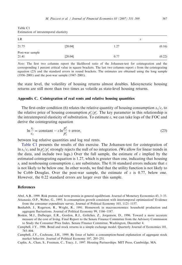
ARTICLE IN PRESS

Table C1

Estimation of intratemporal elasticity

LR �

21.75 [20.04] 1.27 (0.16)

Post-war sample

21.41 [20.04] 0.77 (0.22)

Note: The first two columns report the likelihood ratio of the Johansen-test for cointegration and the

corresponding 1 percent critical value in square brackets. The last two columns report � from the cointegrating

equation (23) and the standard errors in round brackets. The estimates are obtained using the long sample

(1936–2001) and the post-war sample (1947–2001).


the state level, the volatility of housing returns almost doubles. Idiosyncratic housingreturns are still more than two times as volatile as state-level housing returns.

Appendix C. Cointegration of real rents and relative housing quantities

The first-order condition (6) relates the relative quantity of housing consumption st=ct tothe relative price of housing consumption ps

t=pct . The key parameter in this relationship is

the intratemporal elasticity of substitution. To estimate �, we can take logs of the FOC andderive the cointegrating equation

lnst

ct

¼ constant� � lnps

t

pct

þ error, (23)

between log relative quantities and log real rents.Table C1 presents the results of this exercise. The Johansen-test for cointegration of

ln st=ct and ln pst=pc

t strongly rejects the null of no integration. (We allow for linear trends inthe data, and include two lags.) Over the full sample, the estimate of � implied by theestimated cointegrating equation is 1.27, which is greater than one, indicating that housingst and nonhousing consumption ct are substitutes. The 0.16 standard errors indicate that �is not likely to be below one. In other words, we find that the utility function is not likely tobe Cobb–Douglas. Over the post-war sample, the estimate of � is 0.77, below one.However, the 0.22 standard errors are larger over this sample.

References

Abel, A.B., 1999. Risk premia and term premia in general equilibrium. Journal of Monetary Economics 43, 3–33.

Attanasio, O.P., Weber, G., 1995. Is consumption growth consistent with intertemporal optimization? Evidence

from the consumer expenditure survey. Journal of Political Economy 103, 1121–1157.

Benhabib, J., Rogerson, R., Wright, R., 1991. Homework in macroeconomics: household production and

aggregate fluctuations. Journal of Political Economy 99, 1166–1187.

Boskin, M.J., Dulberger, E.R., Gordon, R.J., Griliches, Z., Jorgenson, D., 1996. Toward a more accurate

measure of the cost of living. Final Report to the Senate Finance Committee from the Advisory Commission

to Study the Consumer Price Index. Senate Finance Committee, Washington, December 4.

Campbell, J.Y., 1986. Bond and stock returns in a simple exchange model. Quarterly Journal of Economics 101,

785–804.

Campbell, J.Y., Cochrane, J.H., 1999. By force of habit: a consumption-based explanation of aggregate stock

market behavior. Journal of Political Economy 107, 205–251.

Caplin, A., Chan, S., Freeman, C., Tracy, J., 1997. Housing Partnerships. MIT Press, Cambridge, MA.


Cocco, J., 2005. Portfolio choice in the presence of housing. Review of Financial Studies 18, 535–567.

Cochrane, J.H., 1991a. Production-based asset pricing and the link between stock returns and economic

fluctuations. Journal of Finance 46, 209–237.

Cochrane, J.H., 1991b. Explaining the variance of price–dividend ratios. Review of Financial Studies 5, 243–280.

Cochrane, J.H., 1996. A cross-sectional test of an investment-based asset pricing model. Journal of Political

Economy 104, 572–621.

Cochrane, J.H., Longstaff, F., Santa-Clara, P., 2006. Two trees. Unpublished Working Paper, University of

Chicago, Chicago.

Constantinides, G., Duffie, D., 1996. Asset pricing with heterogeneous consumers. Journal of Political Economy

104, 219–240.

Davis, M., Heathcote, J., 2005. Housing and the business cycle. International Economic Review 46, 751–784.

Dunn, K., Singleton, K., 1986. Modeling the term structure of interest rates under non-separable utility and

durability of goods. Journal of Financial Economics 17, 27–55.

Eichenbaum, M., Hansen, L.P., 1990. Estimating models with intertemporal substitution using aggregate time

series data. Journal of Business and Economic Statistics 8, 53–69.

Eichenbaum, M., Hansen, L.P., Singleton, K., 1988. A time series analysis of representative agent models of

consumption and leisure choice under uncertainty. Quarterly Journal of Economics 103, 51–78.

Flavin, M., Nakagawa, S., 2005. A model of housing in the presence of adjustment costs: a structural

interpretation of habit persistence. Unpublished Working Paper, University of California, San Diego.

Flavin, M., Yamashita, T., 2002. Owner-occupied housing and the composition of the household portfolio.

American Economic Review 92, 345–362.

Glaeser, E.L., Gyourko, J., 2005. Urban decline and durable housing. Journal of Political Economy 113,

345–375.

Goodman, J.L., Ittner, J.B., 1993. The accuracy of home owner’s estimates of house value. Economic Activity

Section Working Paper No. 131, Board of Governors, Washington.

Gordon, R.J., vanGoethem, T., 2004. A century of housing shelter prices: how big is the CPI bias? Unpublished

Working Paper, Northwestern University, Chicago.

Greenwood, J., Rogerson, R., Wright, R., 1995. Household production in real business cycle theory. In: Cooley,

T.F. (Ed.), Frontiers of Business Cycle Research. Princeton University Press, Princeton.

Hall, R.E., 1988. Intertemporal substitution in consumption. Journal of Political Economy 96, 339–357.

Heaton, J., 1993. The interaction between time-nonseparable preferences and time aggregation. Econometrica 61,

353–385.

Heaton, J., 1995. An empirical investigation of asset pricing with temporally dependent preference specifications.

Econometrica 63, 681–717.

Hobijn, B., 2003. On both sides of the quality bias in price indices. Unpublished Working Paper, New York

Federal Reserve, New York.

Jagannathan, R., Wang, Z., 1996. The conditional CAPM and the cross-section of expected returns. Journal of

Finance 51, 3–53.

Kullmann, C., 2002. Real estate and its role in asset pricing. Unpublished Working Paper, University of British

Columbia, Vancouver.

Lettau, M., Ludvigson, S., 2001. Consumption, aggregate wealth and expected stock returns. Journal of Finance

56, 815–849.

Lustig, H., Van Nieuwerburgh, S., 2006. Housing collateral, consumption insurance and risk premia.

Unpublished Working Paper, University of California, Los Angeles.

Malpezzi, S., Turner, B., 2003. A review of empirical evidence on the costs and benefits of rent control.

Unpublished Working Paper, University of Wisconsin, Madison.

McGrattan, E.R., Rogerson, R., Wright, R., 1997. An equilibrium model of the business cycle with household

production and fiscal policy. International Economic Review 38, 267–290.

Mehra, R., Prescott, E., 1985. The equity premium puzzle. Journal of Monetary Economics 15, 145–161.

Menzly, L., Santos, T., Veronesi, P., 2004. Understanding predictability. Journal of Political Economy 112, 1–47.

Ogaki, M., Reinhart, C.M., 1998. Measuring intertemporal substitution: the role of durable goods. Journal of

Political Economy 106, 1078–1098.

Ortalo-Magne, F., Rady, S., 2006. Housing market dynamics: on the contribution of income shocks and credit

constraints. Review of Economic Studies, 73, 459–485.

Prescott, E., 1997. On defining real consumption. Review of Federal Reserve Bank of Minneapolis, May/June,

47–53.


Runkle, D.E., 1991. Liquidity constraints and the permanent-income hypothesis: evidence from panel data.

Journal of Monetary Economics 27, 73–98.

Santos, T., Veronesi, P., 2006. Labor income and asset returns. Review of Financial Studies 19, 1–44.

Stambaugh, R., 1999. Predictive regressions. Journal of Financial Economics 54, 375–421.

U.S. Bureau of Economic Analysis, 1990. Personal consumption expenditures. Methodology Paper No 6. U.S.

Government Printing Office, Washington, DC.

U.S. Bureau of Economic Analysis, 2002. Updated summary NIPA methodologies. hhttp://www.bea.gov/bea/

ARTICLES/2002/10October/1002UpdatedMeth.pdfi.

Yogo, M., 2006. A consumption-based explanation of expected stock returns. Journal of Finance 61, 539–580.

http://www.bea.gov/bea/ARTICLES/2002/10October/1002UpdatedMeth.pdf

http://www.bea.gov/bea/ARTICLES/2002/10October/1002UpdatedMeth.pdf

housing, consumption and asset pricing - stanford …piazzesi/housing.pdf · housing, consumption...

Documents