household formation, housing prices, and public policy impacts

Journal of Public Economics 30 (1986) 145-164. North-Holland

HOUSEHOLD FORMATION, HOUSING PRICES, AND PUBLIC POLICY IMPACTS

Axe1 BORSCH-SUPAN*

John F. Kennedy School of Government, Harvard University, Cambridge, MA 02138, USA

Received April 1985, revised version received March 1986

This paper specifies and estimates a model of housing demand that explicitly includes the decision of individuals to form independent households. Parameter estimates reveal a considerable response of headship rates not only to income but also to housing prices. Analysis of housing policies ignoring the endogeneity of household formation is thus potentially biased. The model is employed to evaluate the effects of a housing voucher program. Simulated responses indicate that such a program creates a substantial additional demand for housing due to its positive impact on the propensity of young and elderly persons to live independently.

1. Introduction

Particularly at the beginning and the end of adult life-cycles, household formation and dissolution are important factors in determining aggregate housing demand. More than half of all adult singles below age 35 and without children, and about a third of all single elderly women, do not live

independently. Given the importance of housing in the economy as a whole, it is

surprising that very little is known about the responsiveness of household formation and dissolution to economic circumstances.

Does the current rise in housing prices discourage the formation of new households? Do children stay longer with their parents when rents are high? Will the decline in housing assistance to the poor precipitate a wave of ‘doubling up’? Was the rise in household formation during the early seventies fostered by the falling real rent level in that period? What are the impacts of a housing voucher program on household size? ’

Conventional housing demand analysis is based on households. House- holds are the sampling unit of almost all available housing data sources. But

*I am greatly indebted to John Pitkin who provided the nucleus-based data sets. Comments from Bill Apgar, Dan McFadden, John Pitkin, Bill Wheaton, the editor, and two anonymous referees are thankfully acknowledged. Financial support was received from the Joint Center of Housing Studies Housing Futures Program. Linda Woodbury greatly improved my English. All remaining errors are mine.

0047-2727/86/$3.50 0 1986, Elsevier Science Publishers B.V. (North-Holland)

146 A. Btirsch-Supan, Household formation

the household is not always the correct decision unit for analyzing of housing demand: rather, the nuclear family or even the adult individual within a composite household decides housing consumption, and housing choices include forming an independent household or merging with another existing household as well as the conventional categories of tenure and size choice.

Sampling the wrong decision unit has major implications for estimation and prediction of housing demand. A sample of households cannot be considered a random sample for the purpose of housing market analysis because households may consist of independent members who combine or separate for reasons endogenous to the housing market. As a statistical consequence, estimation results will be biased due to sample selection, as studied by Heckman (1979). As a practical consequence, prediction of housing market behavior and policy analysis will be biased as well. For instance, if privacy is considered an economic good which is complementary

to housing, then a rising real rent level may induce formation of combined households rather than moves of existing households into lower quality dwellings. Conversely, a housing voucher program may precipitate ‘undoubling’ of large households into several smaller independent households. Finally, the current cuts in spending on public housing programs may greatly increase the number of individuals that give up their independent household status and ‘double up’ as a way to decrease housing expenditures.

2. The framework

New households are formed when existing households split up: children decide to leave their parents’ home, marriages end in divorce, or families that used to live together decide to ‘undouble’. Conversely, some households cease to exist because they merge with another existing household, for instance due to a marriage or doubling up, or because of the decease of a person living alone. Are these mechanisms affected by economic circumstances, in particular by housing market conditions? What are the determinants of household formation?

The early literature on household formation concentrated on two aspects: the rise or decline of the total population size, and the distribution of age and marital status within the population [Campbell (1963), Kobrin (1973, 1976)]. In particular, much interest has been devoted to the dramatic increase in the number of households with only one person. This change is much larger than the change in the distribution of age and marital status alone would predict [Masnick (1983), Alonso (1983)]. Campbell (1963) attributed this discrepancy to ‘the development of a taste for privacy and independence’.

The search for an explanation of this development concentrated on the rise

A. Bksch-Supan, Household formation 141

in real income during the sixties that made privacy and independence affordable. Beresford and Rivlin (1966) Carliner (1975), and Michael, Fuchs

and Scott (1980) present discussions of cross-sectional evidence focusing on this explanation, whereas Maisel (1960), Hickman (1974), and DePamphilis (1977) explore time-series of headship rates to find a positive income effect.

The role of income as the most important explanation of growth in household formation, over and above demographic changes, was put in doubt in the mid-seventies when the rise of real income slowed down considerably. However, in 1975-80, the upward trend in household formation even accelerated relative to 197&75 [Kitagawa (1981), Masnick (1983)]. The falling real rent level in this period’ suggests that not only the income at disposal, but also the price of privacy - the price of housing - may have contributed to the affordability of privacy and independence. A look at recent developments underscores the importance of this hypothesis: in the early 1980s we finally observe household formation leveling off while at the same time real rents started to rise again.

Housing prices as determinants of household headship rates have already been considered by Hickman (1974). He estimates a ‘negligible’ price elasticity and concludes that price effects are not important or cannot be separated from income effects. Ermisch (1981) reports the same findings using a microeconomic model of the determination of household size where the disadvantages of crowding have to be traded off against economies of scale in a multi-person household. However, Hickman’s analysis and Ermisch’s results rest on weak statistical grounds2 and are contradicted by two studies that use aggregate time-series data: Rosen and Jaffee (1981) and Smith, Rosen, Markandya and Ullmo (1982) discovered a highly significant in- fluence of the aggregate rent level on headship rates after controlling for income and demographic characteristics.

The purpose of this paper is to construct a statistical model of household formation devised with the following features: (1) the model treats household formation as a particular form of housing; (2) the model is based on the individual decision-maker; and (3) the model avoids the difficult task of determining household size by behavioral mechanism as Ermisch (1981) did.

The estimation of the resulting structural form tends to be unsatisfactory because of the high noise-to-signal ratio given our poor knowledge about these mechanisms. On the other hand, we seek an approach applicable to data on the microlevel which allows us to use the rich information provided

‘Statistical Abstract of the United States 1980, Table 819: Indexes of Residential Rents in Selected SMSAs: 1970-1980, and Table 811: Consumer Price Indexes - Selected Cities and SMSAs: 196G1979.

‘Hickman does not report standard errors; the behavorial model by Ermisch has very little overall explanatory power, pointing to poor model specification or noisy cross-sectional data.

148 A. Biirsch-Supan, Householdformation

in surveys and to avoid typical biases in the use of grouped data in housing demand studies [Polinsky and Ellwood (1979)].

The central idea is simple: first we split up households into their true underlying decision units - we will call them ‘nuclei’ [Pitkin and Masnick

(1983)] - then we let each nucleus decide among all possible housing alternatives which included owning or renting a dwelling as an independent household as well as living in an already-existing household.

A nucleus consists of a married couple or a single individual and includes their children below a certain age (say, 18 years). Children above this threshold are considered grown-up and, as potential household heads, form new nuclei, even if they (still) live in their parents’ households. Similarly, households that consist of several adults are split up into several nuclei, whether or not members are related to each other. Examples are elderly parents in the household of their children, and room-mates. This construction implicitly assumes death, marriage, and divorce3 to be exogenous from the viewpoint of housing market analysis, but allows for the endogeneity of doubling up and undoubling. It also considers endogenous the decision of adult children to stay at or leave home.

Each nucleus chooses its housing accommodation: it either shares housing within a household composed of several nuclei (dubbed the ‘non-headship’

choice), or heads its own household. In the former case, we do not model the details of the living arrangement; in the latter, the nucleus chooses tenure and dwelling size. We can arrange the resulting seven housing alternatives in the form of a decision tree, as depicted in fig. 1. They will be described in more detail in section 3. The creation of the headship/non-headship dichotomy can be interpreted as a reduced form of Ermisch’s (1981) behavioral model of household production and formation.

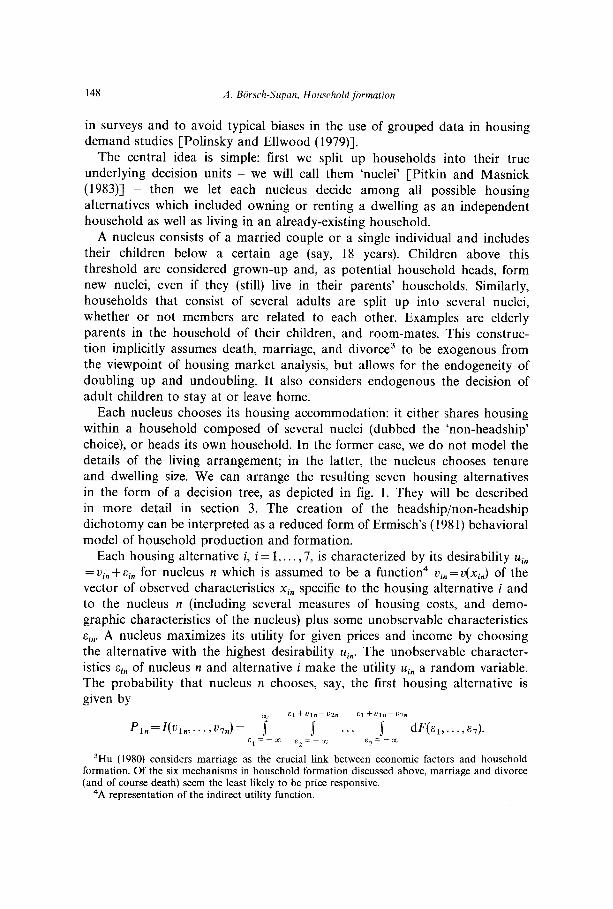
Each housing alternative i, i = 1,. . . ,7, is characterized by its desirability nin

= ui. +Q,, for nucleus n which is assumed to be a function4 Uin = U(Xin) of the vector of observed characteristics Xin specific to the housing alternative i and to the nucleus n (including several measures of housing costs, and demographic characteristics of the nucleus) plus some unobservable characteristics q,,. A nucleus maximizes its utility for given prices and income by choosing the alternative with the highest desirability ui,,. The unobservable characteristics sin of nucleus n and alternative i make the utility uin a random variable. The probability that nucleus n chooses, say, the first housing alternative is given by

El+Uln~Vzn E1 +ul”~V7”

Pi, = I(%. .*, U-in) = 7 s . . . J dF(s,,. . .,E,). E,=pm e =-“. 2 E,=-a)

3Hu (1980) considers marriage as the crucial link between economic factors and household formation. Of the six mechanisms in household formation discussed above, marriage and divorce (and of course death) seem the least likely to be price responsive.

4A representation of the indirect utility function.

A. Bksch-Supan, Household formation 149

Headship: Head Lob.

Tenure: /IL Rent

Ause 1 family houKt

n n n n . .\

n

Size: Small Medium Large All Small Large All Choice: 1 2 3 4 5 6 7 Symbol: OwSmSF OwMeSF OwLaSF ReSFam ReSmAp ReLaAp NoHead

Fig. 1 Housing choices for a nucleus.

Notes: Housing alternatives considered include:

1. OwSmSF: Head, Owner, Small single family home (four or less rooms). 2. OwMeSF: Head, Owner, Medium single family home (five or six rooms). 3. OwLaSF: Head, Owner, Large single family home (seven or more rooms). 4. ReSFam: Head, Renter, Single family home (consolidated, all sizes). 5. ReSmAp: Head, Renter, Small apartment (four or less rooms). 6. ReLaAp: Head, Renter, Large apartment (five or more rooms). 7. NoHead: Non-head (consolidated, all dwelling types).

Once we choose appropriate specifications of the functional form of the indirect utility function u(xin) and the joint distribution function F(E), the choice probabilities Pi,, of each alternative are a well-defined function of all

alternatives’ characteristics xj,, j = 1,. . . , 7. We can therefore evaluate the

responses dP,/8xj, of selecting each housing alternative to changes in the vector of their characteristics. Specifically, we can estimate the response probability of choosing the non-headship alternative with respect to price

changes in the housing market. These responses reflect the price sensitivity of household formation decisions. Since prices are exogenous components of o(xin), these responses do not take account of induced supply changes. The functions Pi, are the discrete analogue to a continuous consumer demand system with exogenous prices.

Without loss of generality’ we chose u(xi,,) as a linear function ui,,=

~,=,,...,,&B” of th e o b served characteristics, where /3 denotes a vector of weights to be estimated. The proper choice of the functional form of the error distribution F(E) is a crucial point of this analysis. Because the housing alternatives in fig. 1 are qualitatively very dissimilar, it is important to model the structure of the hierarchical decision process in fig. 1 properly. This precludes the assumption that the unobserved attributes gin of similar alternatives are independent, hence the usage of the popular multinomial

‘See McFadden (1981) for a thorough exposition of the random utility hypothesis.

150 A. Biirsch-Supan, Household formation

logit model. Instead, we assume that alternatives in common branches of the decision tree in fig. 1 are qualitatively more similar than alternatives in different branches. In addition, we treat the non-headship choice as particularly different from all the other conventional housing choices. This treatment is made operational by allowing for a larger correlation of unobserved characteristics &in within groups of similar housing alternatives as compared to the correlation between groups. We chose a joint distribution function,

F(E) =exp [i[

i$1 exp(si/B,)lB1’a3 + exp(sJlie3

+ j5 exP (02) [

T2’02r3 - exp(.s,)],

from the family of generalized extreme-value distributions that implies the nested logit model proposed by McFadden (1978). It is parameterized by the ‘similarity coefficients’ 0, which reflect the correlation of unobserved attributes within a group of alternatives. 8, corresponds to the group of homeownership alternatives, t32 to apartment rentals, and e3 to all alternatives characterized by independent headship.

A similarity coefficient of one implies that the corresponding within-group

correlation is equal to the between-group correlation. In particular, the nested logit model collapses to the simple multinomial logit model if all similarity coefficients are one. In turn, similarity coefficients smaller than one

indicate common unobserved characteristics within the corresponding group of alternatives.

The resulting choice probabilities have a convenient explicit form:

pin = Pin(XlnP, . . ) X7,P, 0) = P,(Hi) ’ p& 7; 1 Hi) pfiSi 1 T, Hi)

where Hi denotes the headship status, T the tenure, and Si the dwelling size of alternative i. The probability of choosing dwelling size S conditional on headship H and tenure T is

PAS 1 T, H) = ex~GwVT)

c S’ET exP(Xsd/eT)

Denoting the logarithm of the above denominator as yTn, the probability of choosing tenure T conditional on headship H can be written as

pn( T/W = exp (YTneT/eH)

c T’&H exp (yT’neT’ieH) ’

A. Btirsch-Supan, Household formation 151

By repeating this procedure for the logarithm of the above denominator Y,, we obtain the marginal probability of choosing headship status H:

We can estimate the weights /? and the similarity coefficients 9 by maximizing the log-likelihood function:

where j(n) denotes the alternative chosen by nucleus n.

3. The data

The choice among housing alternatives depends on demographic variables (age, sex, marital status, and race of head of nucleus, and the number of children in the nucleus), and financial variables (after-tax user-cost and current nucleus income).6 We pursue the approach of de Leeuw (1971) and Quigley (1976) and assume different demand functions for nuclei with different demographic characteristics. Accordingly, we stratify the sample with the demographic variables. Of all possible strata, this paper examines demand functions for two population groups:

(1) young singles - unmarried white men and women without children, aged 2&35; and

(2) single elderly women - widowed, separated, and divorced white women without children, aged 60 and above.

We concentrate on these two population strata because, in these, household formation is particularly important. The estimates are taken from the Annual Housing Survey SMSA cross-sections 1976-77.’ They are based on three Standard Metropolitan Statistical Areas representing the Northeast, the Sunbelt, and the West Coast - Albany/Schenectady/Troy, New York; Dallas, Texas; and Sacramento, California.

The sampling unit of the Annual Housing Survey is the household. However, the composition of each household is well documented. This allows us to detect other adults in the household as well as their children, and to create a data record for each of these subnuclei in addition to the head nucleus.

6The Annual Housing Survey has no data on wealth, nor does it allow a satisfactory imputation of wealth and permanent income.

‘Albany and Sacramento were sampled in 1977; Dallas in 1976. 1976 Dollar amounts were inflated with the BLS Consumer Price Index, Selected SMSAs, for Dallas.

152 A. BCrsch-Supan, Household formation

Each nucleus chooses a housing alternative from those depicted in lig. 1. Housing alternatives are characterized by the non-head/headship dichotomy, by tenure choice, and by number of rooms as a crude measure of quality and size. ‘Small’ refers to dwellings with up to four rooms, ‘medium’ to dwellings with live or six rooms, and ‘large’ to dwellings with at least seven rooms. Some of the alternatives are rarely chosen, e.g. renting large apartments or single-family homes, and homeownership among young singles, so those alternatives had to be consolidated to allow reliable estimation. No cost data are available for owner-occupied dwellings in multi-family buildings and these alternatives were ‘bmitted from the choice set.8 Table 1 presents the choices observed in our sample and the means of the financial variables. Note the large share of nuclei that do not live independently.

The financial variables, income and user-cost, enter the demand functions directly. Income is defined as the current total gross income of all nucleus members. Income enters the demand functions linearly, interacting with alternative-specific effects. In addition, income influences the out-of-pocket costs of homeowners because federal income tax savings depend on the

marginal tax rate implied by their gross income. User-cost (UC) must be distinguished for renters and owners. For renters,

the user-cost is simply gross rent. For owners, the user-cost has a number of components [for example, see Poterba (1984)]:

I_JC(own) = maintenance + insurance + utility-payments

+ mortgage-rate * debt

+ property tax rate * value -tax savings from federal income tax deductions + T-Bill-rate * equity -rate of appreciation * value,

where the tax savings on the federal income tax is the sum of the local property tax and the mortgage interest, multiplied by the appropriate marginal tax rate depending on such nucleus characteristics as income and number of children. Furthermore, we assume different interest rates on debt and on equity to account for the effect of inflation on fixed rate mortgages.

Owner user-costs consists of two types of cost which the nucleus perceives differently: maintenance, mortgage costs, property taxes, and federal income tax savings are easily perceived costs, whereas capital gains from appreciation are uncertain and opportunity costs of equity are a rather cloudy concept for non-economists. Therefore, we split user-costs into two components:

UC(own) = OOPOCK(own) + RETURN(own),

A. Biirsch-Supan, Household formation 1.53

Table 1

Sample statistics.

(a) Observed market shares of housing alternatives

Market share of housing alternativea

Stratum: NoHead OwSmSF OwMeSF OwLaSF ReSFam ReSmAp ReLaAp

Albany Young singles Single elderly women

Dallas Young singles Single elderly women

Sacramento Young singles Single elderly women

63.3 0.9b 1.2 28.2 6.4 27.6 6.9 16.2 9.9 2.7 23.4 13.5

55.1 2.2 4.8 34.4 3.5 21.3 11.7 31.4 4.9 7.4 18.4 5.0

62.6 4.3 5.1 26.4 1.3 27.5 11.1 22.8 5.6 7.3 24.4 1.4

(b) Sample means of price and income variables

Out-of-pocket user-costsc





1.00 4.23b 2.85 2.08 2.45 1.02 1.64 3.76 6.13 2.81 1.98 2.39

1.00 4.55 2.53 2.26 2.92 0.98 1.96 3.29 8.52 2.46 2.19 2.93

0.95 4.06 2.58 2.03 2.83 0.97 2.32 3.65 6.55 2.53 1.94 2.83

Return from equity’

Stratum: OwSmSF OwMeSF OwLaSF Current income’




4.23b 5.20 2.23 1.65 2.35 5.32

5.80 6.65 3.15 3.59 4.00 5.57

5.67 5.16 3.13 3.44 4.07 6.00

aPercentage of observed housing choices, Annual Housing Survey, 197677. “For young singles, the three homeownership choices are consolidated. “Yearly, in 1000 dollars. Annual Housing Survey, 1976-77.

154 A. Bfirsch-Supan, Household formation

where ‘out-of-pocket cost’ is composed of:

OOPOCK(own) = maintenance + insurance + utility-bills + local property tax + mortgage-rate * debt -federal income tax savings;

and the return from the asset homeownership is defined as:

RE TURN(own) = expected rate of appreciation * value -T-Bill-rate * equity

If housing demanders were perfectly rational, the coefficients for OOPOCK and RETURN would be of equal magnitude and opposite sign. For renters,

we set RETURN to zero.

The Annual Housing Survey contains precise data for the components of out-of-pocket costs. The return variable is constructed with external information. As a simple substitute for expected yearly appreciation, we converted the difference in house values between the Annual Housing Survey 197677 and the 1970 Census of Housing into yearly rates. This rate varies by SMSA and by type of dwelling. The opportunity costs of holding equity in housing are calculated from the value-to-loan ratio observed in the Annual Housing Survey, multiplied by the interest on live-year U.S. treasury bills.’

When households are decomposed into separate nuclei, the explanatory variables have to be split up according to this partition. The Annual Housing Survey reports all demographic variables and the most important income sources by individual household member.” For out-of-pocket costs, it suggests itself that the nuclei pay their shares in proportion’l to the number of adults and children in the nucleus.12 However, appreciation gains

‘A more satisfactory approach would be to impute the cost data for multifamily dwelling from hedonic regressions [Borsch-Supan (19X5)], or to explicitly model the missing alternatives in the definition of the choice probabilities. The problem is a minor one for Dallas and Sacramento, where these alternatives count for only 0.5 and 0.8 percent of all choices; it is more serious for Albany, where 6.9 percent of all nuclei chose units in cooperatively owned multifamily buildings.

‘Unfortunatly, appreciation rates and equity costs suffer from data problems: loan-to-value ratios are often not reported, making imputations necessary, and the available appreciation rates vary only by SMSA, but not within SMSA.

“‘Some transfer income is only reported by household. Given the demographic characteristics of each person, it is possible to employ a fairly accurate income allocation scheme for these income categories.

“This sharing scheme is realistic for roommates, less so for adult children living in their parents’ household. However, they incur non-monetary costs in the form of household help, etc.

“Note that for a common price for all housing units this relation establishes an identity between the prices of non-heads and heads. In this case, the price coefficients would not be identified in certain functional forms of the demand equations. One sufficient condition for identification independent of the functional form is the presence of economies of scale in the formation of larger households. In fact, these economies are likely to exist and seem to be a major attraction to share accommodations.

A. BCrsch-Supan, Household formation 155

(RETURN) in the case of homeownership are not shared and benefit only the actual owner of the unit. The sample averages of the price and income variables are displayed in table 1.

Given the cross-sectional data, the choice among the housing alternatives is a hypothetical one. We observe each nucleus with its chosen alternative and its attributes, but we do not observe the attributes of the alternatives that the nucleus rejected. We impute the current spot market prices of rejected alternatives using the average prices observed in a cross-section of all recent movers. This is motivated by the notion that a household collects its information on prices of other units by skimming through advertisements in newspapers and by listening to the experiences of friends and neighbors who have just moved. l3

4. Price responsiveness of household formation

We have constructed a demand system of seven housing alternatives, depicted in fig. 1, with demand functions defined by the nested logit model of section 2 which depend on the demographic and financial variables specified in the preceding section. We will focus on the seventh alternative of not heading an independent household to study household formation.

We did not attempt to construct a fully simultaneous housing market model. This will not lead to considerable simultaneity bias for the study of household formation on the level of individual nuclei. Supply for newly formed households in an essentially stable population is provided mostly by conversion of existing units, less so by relatively inelastic new construction.t4 If demand is easily accommodated by supply, we can estimate the demand functions without simultaneity bias. We will test this assumption by comparing different supply regimes at the end of this section.

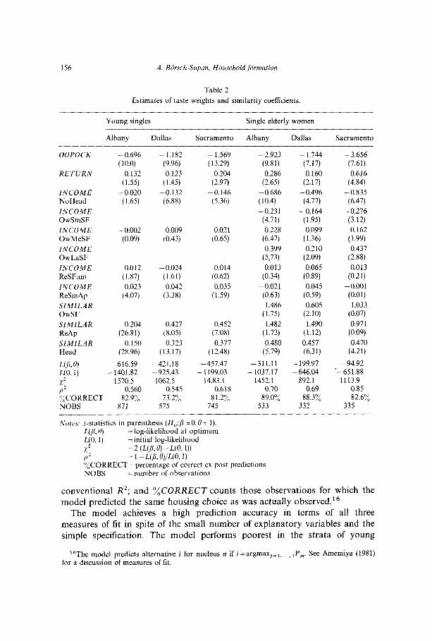
We estimate the price responsiveness of household formation by maximizing the likelihood function described in section 2. This yields consistent estimates of the taste parameters fl” that weight the characteristics x% entering the indirect utility function Vi* and of the similarity coefficients 0 that generate the decision tree in fig. 1. The parameter estimates and summary statistics are presented in table 2. Three scalar measures of performance or fit are used: x2 measures the improvement of the log- likelihood from /?=O and fI= 1 to the optimal parameters by a chi-squared distributed statistic;15 p2 transforms this measure into an equivalent to the

r3For the hypothetical loan-to-value ratios, we assume a 20 percent downpayment for young singles, and 99 percent for elderly households, which takes into account the availability of mortgage loans to the different age groups. This assumption is not critical to the estimates, and is confirmed by cross-tabulations of recent movers.

“Examples are college towns where we observed the repartitioning of existing buildings into smaller units, and the recent reduction of transfer payments to the urban poor in the United States which led to an almost instantaneous ‘doubling up’ in poor neighborhoods.

“The degrees of freedom are the number of parameters estimated.

156 A. Biirsch-Supan, Household formation

Table 2

Estimates of taste weights and similarity coefficients.

Young singles Single elderly women

Albany Dallas Sacramento Albany Dallas Sacramento

OOPOCK -0.696 - 1.182 (10.0) (9.96)

RETURN 0.132 0.123 (1.55) (1.45)

INCOME - 0.020 -0.132 NoHead (1.65) (6.88)

INCOME OwSmSF

INCOME - 0.002 0.009 OwMeSF (0.09) (0.43)

INCOME OwLaSF

INCOME 0.012 - 0.024 ReSFam (1.87) (1.61)

INCOME 0.023 0.042 ReSmAp (4.07) (3.38)

SIMILAR OwSF

SIMILAR 0.204 0.427 ReAp (26.81) (8.05)

SIMILAR 0.150 0.323 Head (28.96) (13.17)

L(/(> 0) -616.59 -421.18

L(O,l) - 1401.82 - 925.43

x2 1570.5 1062.5

P2 0.560 0.545 %CORRECT 82.9% 73.2% NOBS 871 575

- 1.569 (13.29)

0.204 (2.97)

-0.146 (5.36)

0.021 (0.65)

0.014 (0.62)

0.035 (1.59)

0.452 (7.08)

0.377 ( 12.48)

-457.47 - 1199.03

14.83.1 0.618

81.2% 745

- 2.923 (9.81)

0.286 (2.65)

- 0.686 (10.4)

-0.231 (4.71)

0.228 (6.47)

0.399

(5,73) 0.013

(0.34)

-0.021 (0.63)

1.486 (1.75)

1.482 (1.73)

0.480 (5.79)

-311.11 - 1037.17

1452.1 0.70

89.0% 533

- 1.744 (7.17)

0.160 (2.17)

- 0.496 (4.77)

-0.164 (1.95)

0.099 (1.36)

0.210 (2.09)

0.065 (0.89)

0.045 (0.59)

0.605 (2.10)

1.490 (1.12)

0.457 (6.31)

- 199.97 - 646.04

892.1 0.69

88.3% 332

- 3.656 (7.61)

0.616 (4.84)

-0.835 (6.47)

- 0.276 (3.12)

0.162 (1.99)

0.437 (2.88)

0.013 (0.21)

-0.001 (0.01)

1.033 (0.07)

0.971 (0.09)

0.470 (4.21)

- 94.92 ‘-651.88

1113.9 0.85 82.6%

335

Notes: t-statistics in parenthesis (H,:o=O, IV= 1).

L(B, 0) = log-likelihood at optimum

UO> 1) = initial log-likelihood

X2 = 2 (UP, 0) - UO, I)) P2 = 1 - L(B, WUO, 1) %CORRECT=percentage of correct ex post predictions NOBS =number of observations

conventional R2; and ‘ACORRECT counts those observations for which the model predicted the same housing choice as was actually observed.16

The model achieves a high prediction accuracy in terms of all three measures of fit in spite of the small number of explanatory variables and the simple specification. The model performs poorest in the strata of young

16The model predicts alternative i for nucleus n if i=argmaxj= ,,..., ,P,“. See Amemiya (1981) for a discussion of measures of fit.

A. Bdrsch-Supan, Household formation 157

singles. This static model can hardly capture changes in housing consump-

tion during the period when young nuclei are establishing their own

existence. These strata are also very heterogeneous and include children still living with their parents, student room-mates, and singles in their thirties.

The main substantive result is the significance of the two price variables in all strata. The out-of-pocket costs (OOPOCK) are highly significant, while the variable measuring the return from investing equity into homeownership (RETURN) is weaker. Note that the hypothesis of rationality - i.e. equal magnitude and opposite signs for the coefficients of OOPOCK and RETURN - is rejected; considerably greater weight is given to easily perceived out-of-pocket costs as opposed to expected appreciation minus

equity costs.’ 7 RETURN is least significant for young singles, the strata

most affected by liquidity constraints, where the rationality hypothesis is most inappropriate and the omission of a wealth variable is most severe.

The income terms have a threefold function. First, they reflect the relative price of housing with respect to all other goods. In addition, they indicate the attractiveness of the various alternatives relative to large rented apart-

ments - the excluded housing alternative - measured in money terms. In the absence of any other alternative-specific effects, they also picks up all other non-measured advantages and disadvantages of the included alternatives relative to large rented apartments. One should therefore only carefully draw conclusions about pure income effects.‘* The attractiveness of the alternatives measured by the taste weights of income dummies corresponds to a priori

assessment. Almost all similarity coefficients are significantly different from one.19 This

tells us that the hierarchical structure of the decision tree in fig. 1 is indeed an important feature of housing choices, in particular because of the

inclusion of the non-headship alternative To gain some intuition for the magnitudes of the coefficients, and to

measure the effects of the explanatory variables xjn on each housing choice

Pi, separately, we calculate the elasticities d log(PJ8 log (Xj,) in tables 3 and 4. First, we compare (in table 3) the own price and income elasticities across strata. The following patterns emerge: headship rates are responsive to the cost of shared living arrangements in both strata of singles and single elderly women, with a substantially larger response to all economic factors in the elderly strata. As a regional pattern, the strata of young singles and single

“However, one should keep in mind that the RETURN variable was imputed and thus subject to potential data errors.

‘*Introduction of alternative-specific dummies reduces the income parameters, but leaves the price variables virtually constant. Because the focus of the simulations below will be on relative prices rather than on income, we avoided the costly inclusion of alternative-specific dummies.

“Their t-statistics are evaluated around one. Two similarity coefficients are significantly larger than one. Using a criterion developed in Bijrsch-Supan (1985), they are nonetheless compatible with stochastic utility maximization.

158 A. BSrsch-Supan, Household formation

Table 3

Own price and income elasticities of market shares.

Market share of housing alternativea

Variable NoHead OwSmSF OwMeSF OwLaSF ReSFam ReSmAp ReLaAp

Albany Young singles:

OOPOCK RETURN INCOME

Single elderly women: OOPOCK RETVRN INCOME

Dallas Young singles:


Single elderly women: OOPOCK RETURN INCOME

Sacramento Young singles:


Single elderly women: OOPOCK RETURN INCOME

-0.395 - 19.596b - 12.913 - 2.463 - 1.227 0.0 3.675 0.0 0.0 0.0

- 0.083 -0.591 -0.101 0.238 -0.343

- 2.430 0.0

- 3.694

- 0.632 0.0

-C 669

- 1.431 0.0

- 2.823

-0.728 - 16.459 - 10.046 - 3.563 -9.519 0.0 2.939 0.0 0.0 0.0

-0.513 0.279 0.181 0.468 0.064

-2.814 0.0

-4.871

_

- 6.984 -7.529 - 11.861 - 16.940 - 5.919 -6.016 -0.914 -0.292 -0.418 0.0 0.0 0.0 - 1.284 0.359 0.973 - 0.428 -0.137 - 0.664

- 5.806 - 8.680 - 24.426 - 8.964 -5.162 -4.867 0.816 0.682 1.016 0.0 0.0 0.0

- 1.958 0.457 1.478 0.341 0.005 -0.164

12.898 - 12.540 -23.002 - 19.015 - 10.477 - 10.964 2.759 1.711 2.316 0.0 0.0 0.0

- 2.002 0.548 2.146 -0.147 -0.326 -0.320

- 16.494 - 8.392 -3.031 -7.641 2.165 0.0 0.0 0.0

-0.037 -0.710 0.625 - 0.030

“Price and income elasticities refer to a percentage change of the fraction of nuclei choosing a housing alternative when OOPOCK or RETURN in this alternative or INCOME of each nucleus is raised by 1 percent.

bFor young singles, the three homeownership choices are consolidated.

elderly women in Albany are the least price-responsive, especially in the owner alternatives, confirming our a priori assessment of inertia and mobility across the country. Return from the homeownership asset exhibits a strong life-cycle behavior: it is higher for young people with a long decision horizon than for the elderly. In general, elasticities in rarely chosen alternatives are of very large magnitudes, a consequence of the nonlinearity of the model.

Table 4 is the core result of this paper and presents the cross-elasticities of the non-headship choice, that is the response of household formation to individual price changes in the housing market. The closest substitute for the non-headship alternative is small rental units, as expected. Their large cross- elasticities reflect the responsiveness of household formation to the rental

A. BCrsch-Supan, Household formation 159

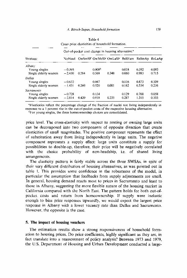
Table 4

Cross price elasticities of household formation.





-0.395 0.008b 0.018 0.392 0.093 - 2.430 0.284 0.568 0.348 0.060 0.983 0.715

-0.632 0.047 0.116 0.873 0.109 ~ 1.431 0.260 0.520 0.081 0.162 0.534 0.236

-0.728 0.134 0.129 0.768 0.058 -2.814 0.420 0.918 0.235 0.287 1.315 0.103

Out-of-pocket cost change in housing alternative.”

aElasticities reflect the percentage change of the fraction of nuclei not living independently in response to a 1 percent rise in the out-of-pocket costs of the respective housing alternative.

‘For young singles, the three homeownership choices are consolidated.

price level. The cross-elasticity with respect to renting or owning large units

can be decomposed into two components of opposite direction that create elasticities of small magnitudes. The positive component represents the effect

of substitution away from living independently in large units. The negative component represents a supply effect: large units constitute a supply for possiblilities to double-up, therefore, their price will be negatively correlated with the choice probability of non-headship, i.e. of shared living

arrangements. The elasticity pattern is fairly stable across the three SMSAs, in spite of

their very different distribution of housing alternatives, as was pointed out in table 1. This provides some confidence in the robustness of the model, in

particular the assumption that feedbacks from supply adjustments are small. In general, housing demand reacts most to prices in Sacramento and least to

those in Albany, suggesting the more flexible nature of the housing market in California compared with the North East. The pattern holds for both out-of- pocket costs and return from homeownership. If supply were inelastic enough to bias price responses upwardly, we would expect the largest price response in Albany with a lower vacancy rate than Dallas and Sacramento. However, the opposite is the case.

5. The impact of housing vouchers

The estimation results show a strong responsiveness of household formation to housing prices. Do price coefficients, highly significant as they are, in fact translate into a reassessment of policy analysis? Between 1973 and 1979, the U.S. Department of Housing and Urban Development conducted a large-

160 A. Btirsch-Supan, Household formation

scale experimental housing allowance program.” Somewhat surprising is the fact that almost all analysis of this experiment ignored the feedback of housing allowances on household formation. We will use the estimation results of the preceding section for a simulation of a general housing voucher program that was motivated by the experimental housing allowance program and is now proposed as a substitute for the current Section 8 program. This simulation is intended to produce answers to questions of the following nature: How much ‘undoubling’ of composite households will be generated by the distribution of housing allowances ? What is the participation after controlling for household formation? Where in Sweeney’s (1974) commodity hierarchy of the housing market would we expect shortages or price pressure in response to housing allowances?

This experiment is an exercise in comparative statics and has to be interpreted as a long-run response, leading to a new steady state equilibrium. Furthermore, the results are based on partial analysis of only the demand side in the preceding sections. Thus, we implicitly assume a perfectly elastic housing supply and disregard all transitional phenomena like inertia of mobility and transaction costs.21 We also disregard any secondary price effects induced by the voucher program which are likely to offset some of the first round effects.

The simulation assumes the so-called housing gap formula for the calcu- lation of the housing vouchers. First, for each family size and site a

benchmark rent is calculated, representing the ‘fair cost of standard housing’. Then a minimum standard of quality is established, and only dwellings above

this standard are eligible for the subsidy. Finally, a linear tax is levied on the allowances in such a way that households with no (adjusted) income will receive the full rent for standard housing, whereas households above a certain income level will receive no allowances at all.

If the minimum standard is measured as a fraction M of the fair cost of standard housing R*, and the linear tax rate is denoted by p, then the housing allowance for a renter household with income Y and actual rent R

is:

R*-BY, ifRzaaR* and Y<R*/fl

0, otherwise.

To perform a realistic experiment, we used the parameter settings c(, fi, and R* from the Experimental Housing Allowances Program.22 Housing al-

“‘Kennedy (1980) describes in detail the design of the program. Bradbury and Downs (1981) give a good survey of the subsequent discussion and critique.

“Compare Venti and Wise (1984) for an analysis of transaction costs. 22They are: cc=O.7, fl=O.25, and R* from the Pittsburgh demand experiment inflated by a

yearly as well as an inter-SMSA rent index to our sample SMSAs and periods.

A. Btirsch-Supan, Iiou.sehold,fi~rmc~tion 161

lowances introduce non-linearities in the budget set [Venti and Wise (1984)].

They can be handled elegantly in discrete choice models by changing the prices of each housing alternative differently rather than by adding the allowances to the income of the household.

Table 5 lists the predicted market shares of each housing alternative before and after the introduction of the housing voucher program. The shares are calculated as means of the individual choice probabilities Pi,. Since the model is static and partial, the differences between the columns of table 5 reflect changes between steady states that ignore transitional frictions as well as induced supply responses.

Given these caveats, our main result is the strong impact of housing allowances on headship rates: about half of the people who lived in some kind of shared accommodations created their own households in response to

the distribution of housing vouchers. Most of the nuclei in the strata of young singles have little or no income. Therefore, if they decide to become independent households, their rent net of the housing allowance is virtually zero. More surprising is the strong response in the strata of single elderly women, where the non-head share is far less and the income higher than

among the young singles. The share of elderly not living independently is nevertheless drastically reduced in response to the subsidy. Thus, household

Table 5

Response of market shares of housing alternatives.

Market share of housing alternative”

Albany Dallas Sacramento

Without With Without With Without With housing housing housing housing housing housing vouchers vouchers vouchers vouchers vouchers vouchers

Young singles NoHead OwSmSF OwMeSF OwLaSF ReSFam ReSmAp ReLaAp

Single elder2y women NoHead OwSmSF OwMeSF OwLaSF ReSFam ReSmAp ReLaAp

63.3 1 47.80 55.07 32.26 62.62 30.67

0.92b 0.92 2.24 2.19 4.25 4.09

1.23 1.59 4.78 9.13 5.08 7.72 28.15 40.41 34.38 50.46 26.42 53.96

6.37 9.28 3.53 5.96 1.63 3.56

27.57 13.00 21.30 10.05 27.45 10.68 6.94 3.87 11.65 5.62 11.05 9.46

16.02 13.98 31.44 28.75 22.8 1 22.32 9.85 9.09 4.86 4.53 5.62 5.58 2.13 2.86 7.37 9.53 7.29 7.77

23.40 36.36 18.42 30.39 24.37 41.60 13.48 20.84 4.96 11.33 1.40 2.59

“First column: predicted percentages of housing alternatives (baseline prediction). Second column: predicted percentages of housing alternatives when housing vouchers

of amount R* -pY are distributed. “For young singles, the three homeownership choices are consolidated.

162 A. Bckch-Supan, Household,formution

formation is an important endogenous mechanism in the housing market that cannot simply be ignored when evaluating the impacts of public policy. Conventional housing demand analysis without consideration of the household formation response would have predicted an increase in the market share of higher quality/larger size units and a corresponding decrease in the shares at the bottom of Sweeney’s (1974) quality scale. However, many large composite households split into smaller households and precipitate an increased demand for small units that not only compensates for but indeed outweighs the above shift away from small units. A supplemental short-run supply program with the intention of easing demand pressure in the submarket of large units, where conventional analysis predicts shortages, would largely fail because it would be geared to the wrong segment of the housing market.

The model also generates a matrix of individual transitions in response to

housing allowances. It tabulates the number of predicted moves per 1000 nuclei into the rental sector by previous housing choice and includes the newly formed renter households. A move of an individual nucleus is predicted when the housing choice of maximum desirability under the program is different from the preferred choice without housing vouchers. Almost all newly formed households move to small rental units. Within the rental sector, only few moves occur. When the model is applied to the entire population, not only to our two test strata, the resulting low mobility rates

(Albany 0.047, Dallas 0.057, Sacramento 0.055) are very close to those measured in the demand part of the experimental housing allowance

program (Pittsburgh 0.045 and Phoenix 0.101),23 and reiterate the lesson about little participation in programs that require moving. Note again the difference in the response between the Northeast and the Southwest.

Finally, the distribution of housing vouchers for renter households changes the balance in the tenure choice in favor of renting. As a response, we observe a relatively large number of moves from the owner-occupied to the rental housing market. For some single elderly women, the allowances are presumably a final incentive to dispose of the now oversized family home. The mobility rates for the shift from owning to renting induced by the allowances are between 0.125 for Sacramento and 0.189 for Albany. Note the lower rate for Sacramento, reflecting the high valuation of owner-occupany in the West relative to the Northeast.

6. Conclusions

The main conclusions from the baseline estimates and from the housing voucher simulation is the strong response of headship rates to relative

*%ee MacMillan (1978).

A. Bb’rsch-Supan, Household formation 163

housing prices. In the two strata examined, household formation cannot be treated as a mechanism which is exogenous to the housing market.

In the choice among conventional housing alternatives, the out-of-pocket component of user-costs has a larger weight in household utility than the return from equity invested in homeownership, pointing to a large discount on expected appreciation. The weights show the expected pattern across life- cycles and across regions.

The model performs well in terms of lit and prediction accuracy. The

results have a fairly stable pattern across SMSAs. In the case where our simulation can be validated by the Experimental Housing Allowance Pro- gram, the results are very close. All this gives us confidence in the robustness of the model and the validity of our conclusions.

However, caveats should be made that concern the interpretation of a pure demand model based on cross-sectional data. The model ignores all second round market effects. Ignoring supply adjustments for newly formed households was shown to be harmless. We also ignore all intertemporal effects that might produce price dispersion. For instance, spurious price elasticities are estimated when sitting tenants in rental housing receive ‘tenure discounts’ by paying less than the prices paid by recent movers. Such price dispersion was estimated by Malpezzi, Ozanne and Thibodeau (1980) as 25 percent in Albany, 5 percent in Dallas, and 7.5 percent in Sacramento. Even after subtracting these percentages from the price coefficients, the elasticities and simulation responses remain very large. Thus, our main conclusion is not affected: household formation is highly responsive to housing prices, with important implications for public policy.

References

Alonso, William, 1983, The demographic factor in housing for the balance of this century, in: Michael A. Goldberg and George W. Gerr, eds., North American housing markets at the transition into the twenty-first century (Ballinger, Cambridge, MA).

Ameniya, Takeshi, 1981, Qualitative reponse models: A survey, Journal of Economic Literature 19, 14381536.

Beresford, John C. and Alice M. Rivlin, 1966, Privacy, poverty, and old age, Demography 3, 247-258.

Borsch-Supan, Axel, 1985, Tenure choice and housing demand, in: Konrad Stahl and Raymond Struyk, eds., U.S. and German housing markets: Comparative economic analysis (The Urban Institute Press, Washington, DC), 55-114.

Bradbury, Katherine L. and Anthony Downs, 1981, Do housing allowances work? (Brookings Institution, Washington, DC).

Campbell, Burnham O., 1963, Long swings in residential construction: The postwar experience, American Economic Review 53, 508-518.

Carliner, Geoffrey, 1975, Determinants of household headship, Journal of Marriage and the Family 37, 28-38.

DePamphilis, Donald M., 1977, The dynamics of household formation, Business Economics 12, 18-21.

de Leeuw, Frank, 1971, The demand for housing: A review of the cross-section evidence, Review of Economics and Statistics 53. l-10.

164 A. Btirsch-Supan. Ilmsehold Jormation

Ermisch, John F., 1981, An econometric theory of household formation, Scottish Journal of Political Economy 28, l-19.

Heckman, James J., 1979, Sample selection bias as a specification error, Econometrica 47, 153-161. Hickman, Bert G., 1974, What became of the building cycle? in: Paul A. David and melvyn W.

Reder, eds., Nations and households in economic growth: Essays in honor of Moses Abramovitz (Academic Press, New York), 291-314.

Hu, Joseph C., 1980, An econometric model of household headship, Paper prepared for the Southern Regional Demographic Group.

Kennedy, Steven D., 1980, Final report of the housing allowance demand experiment (Abt Associates, Cambridge, MA).

Kitagawa, Evelyn M., 1981, New life-styles: Marriage patterns, living arrangements, and fertility outside of marriage, Annals of the American Academy of Political and Social Science 453, l-27.

Kobrin, Frances E., 1973, Household headship and its changes in the United States 194&60, 1970, Journal of the American Statistical Association 68, 793-800.

Kobrin, Frances E., 1976, The fall in household size and the rise of the primary individual in the United States, Demography 13, 127-138.

MacMillan, Jean, 1978, Draft report on mobility in the housing allowance demand experiment (Abt Associates, Cambridge, MA).

Maisel, Sherman J., 1960, Changes in the rates and components of household formation, Journal of the American Statistical Association 55, 268-283.

Malpezzi, Steven, Larry Ozanne and Thomas Thibodeau, 1980, Characteristic prices of housing in fifty-live metropolitan areas (The Urban Institute, Washingtom DC).

Masnick, George, 1983, The demographic factor in household growth (Joint Center for Urban Studies of MIT and Harvard University, Cambridge, MA).

McFadden, Daniel, 1978, Modelling the choice of residential location, in: Arne Karlgvist, ed., Spatial interaction theory and residential location (North-Holland, Amsterdam).

McFadden, Daniel, 1981, Econometric models of probabilistic choice, in: Charles F. Manski and Daniel McFadden, eds., Structural analysis of discrete data with econometric applications (MIT Press, Cambridge, MA).

Michael, Robert T., Victor R. Fuchs and Sharon R. Scott, 1980, Changes in the propensity to live alone 1950-1976, Demography 17, 39-56.

Pitkin, John and George Masnick, 1983, The relationship between heads and nonheads in the household population: An extension of the headship rate method, in: John Pitkin and George Masnick, eds., Family demography: Methods and their application (Joint Center for Urban Studies of MIT and Harvard University, Cambridge, MA).

Polinsky, A. Mitchell and David T. Ellwood, 1979, An empirical reconciliation of micro and grouped estimates for housing, Review of Economics and Statistics 61, 199-205.

Poterba, James M., 1984, Tax subsidies to owner occupied housing: An asset market approach, Quarterly Journal of Economics 99, 729-752.

Quigley, John M., 1976, Housing demand in the short run: An analysis of polytomous choice, Yale University Working Paper.

Rosen, Kenneth T. and Dwight M. Jafee, 1981, The demographic demand for housing: An economic analysis of the household formation process, Paper prepared for the American Economic Association Meetings.

Smith, Lawrence B., Kenneth T. Rosen, Anil Markandya and Pierre-Antoine Ullmo, 1982, The demand for housing, household headship rates, and household formation: An international analysis, Center for Real Estate and Urban Economics Working Paper 55 (University of California, Berkeley).

Sweeney, James L., 1974, A commodity hierarchy model of the rental housing market, Journal of Urban Economics 1, 288-323.

Venti, Steven F. and David A. Wise, 1984, Moving and housing expenditure: Transactions cost and disequilibrium, Journal of Public Economics 29, 207-243.

household formation, housing prices, and public policy impacts

Documents