holographic ferromagnetism and non-relativistic charged hydrodynamics
TRANSCRIPT
HOLOGRAPHIC FERROMAGNETISM
AND
NON-RELATIVISTIC CHARGED
HYDRODYNAMICS
A REPORT
submitted in partial fulfillment of the requirements
for the award of the dual degree of
Bachelor of Science – Master of Science
in
PHYSICS
by
AKASH JAIN
(Roll No. 09005)
DEPARTMENT OF PHYSICS
INDIAN INSTITUTE OF SCIENCE EDUCATION AND
RESEARCH BHOPAL
BHOPAL - 462066
April 2014
Certificate
This is to certify that Akash Jain, BS-MS (Physics), has worked on the disserta-
tion entitled ‘Holographic Ferromagnetism and Non-Relativistic Charged
Hydrodynamics’ under my supervision and guidance. The content of the thesis
is original and has not been submitted elsewhere for the award of any academic
or professional degree.
April 2014
IISER Bhopal
Dr. Suvankar Dutta
Assistant Professor, Dept. of Physics
IISER Bhopal
Committee Member Signature Date
Academic Integrity and Copyright Disclaimer
I hereby declare that this thesis is my own work and, to the best of my knowledge,
it contains no materials previously published or written by another person, or
substantial proportions of material which have been accepted for the award of any
other degree or diploma at IISER Bhopal or any other educational institution,
except where due acknowledgement is made in the thesis.
I certify that all copyrighted material incorporated into this thesis is in compliance
with the Indian Copyright Act (1957) and that I have received written permission
from the copyright owners for my use of their work, which is beyond the scope of
the law. I agree to indemnify and save harmless IISER Bhopal from any and all
claims that may be asserted or that may arise from any copyright violation.
April 2014
IISER Bhopal
Akash Jain
BS-MS (Physics), IISER Bhopal
– ii –
Preface
This text is a brief report on the work I have been involved in as my master’s
final year thesis project, carried out at Indian Institute of Science Education and
Research (IISER), Bhopal from May 2013 to April 2014, under the supervision of
Dr. Suvankar Dutta, Assistant Professor, Dept. of Physics, IISER Bhopal.
The report is divided into two parts: Holographic Ferromagnetism and Non-
relativistic Charged Hydrodynamics. The first part (Holographic Ferromagnetism)
concerns the study of ferromagnetic properties of a conformal field theory in the
context of the AdS/CFT conjecture in String Theory. The work has been pub-
lished in the Journal of High Energy Physics (JHEP) [1]. In this report we present
the main idea of this work and physical aspects of our results. A rigorous and tech-
nical discussion can be found in the aforementioned research article.
In Part-II (Non-relativistic Charged Hydrodynamics) we try to understand differ-
ent transport properties of a parity-odd, non-relativistic charged fluid in presence
of background electro-magnetic fields. Especially, we construct a consistent en-
tropy current for the non-relativistic fluid and impose constraints on the various
transport coefficients from the positivity of local entropy production. A preprint
of this work can be found on arXiv [2]. Here again, most of the technical issues
have been omitted to keep the report accessible to a broader audience.
Interested readers can jump to either of the parts directly, as none of them impair
the readability of other. However within a part, it is suggestive to go through the
‘Introduction and Background’ section to begin with. Each part has a ‘Discussion’
section where we summarise our main results and scopes for further analysis. The
report has six appendices, four belonging to Part-I and two to Part-II. There we
discuss some of the related but fairly sidelined topics from the main text.
I hope the readers will find the report quite interesting and fairly accessible. Any
queries or clarifications can be directed to [email protected].
Akash Jain
April 2014, IISER Bhopal
– iii –

Acknowledgements
First and foremost, I would like to present my sincere gratitude towards my MS
thesis supervisor, Dr. Suvankar Dutta for his constant support and motivation
throughout the project.
I would also like thank Dr. Nabamita Banerjee (Assistant Professor, Dept. of The-
oretical Physics, IACS Kolkata) for taking time out of her schedule and providing
me with invaluable academic guidance and insights.
A special thanks to my another collaborator Dr. Dibakar Roychoudhury.
I find myself fortunate to have an opportunity to work under such friendly super-
vision, and am grateful to the unparalleled efforts my supervisor and collaborators
for making my first research experience so wonderful.
I am thankful to my colleagues, especially Pratik Roy and Rahul Soni for vital
discussions and aid, which helped me gain a better understanding of the subject
matter and motivated me to continue the hard work.
I would like to thank INSPIRE, Department of Science and Technology, MHRD,
Govt. of India for their generous funding throughout my graduation. I am also
grateful to the Department of Physics, IISER Bhopal for their support and pro-
viding me with the required infrastructure and facilities to successfully complete
my graduation and carry out this project.
Finally I would like to thank all my friends, family members and my parents
for their moral support and motivation, which enabled me to concentrate better
towards my academia.
– iv –
Abstract
In the first part of this thesis, we study thermodynamic and magnetic properties of
a conformal field theory living on the surface of a two-sphere using the AdS/CFT
correspondence. The correspondence is an efficient tool to study properties of a
strongly coupled quantum field theory in terms of its weakly coupled super-gravity
dual. We find that our field theory exhibits a ferromagnetic-type phase transition.
At high temperature and in absence of external magnetic field the system has zero
magnetization, and below a critical temperature it spontaneously picks up an ar-
bitrary direction and develops a constant magnetization. Unlike a ferromagnetic
system however, we find a discontinuity in magnetization at the transition temper-
ature. We also study the magnetic susceptibility of various thermodynamic phases
of the system and find that depending on temperature and applied magnetic field,
a phase is either paramagnetic or diamagnetic.
In the second part, we aim to study transport properties of a parity-odd, non-
relativistic charged fluid in presence of background electric and magnetic fields.
To obtain the stress tensor and charge current of the non-relativistic system, we
start with the most generic relativistic fluid living in one higher dimension, and
reduce the constituent equations of the relativistic system along the light-cone
direction. This mechanism is known as light-cone reduction. In the similar way,
reducing the equation satisfied by the entropy current of the relativistic theory we
obtain a consistent entropy current for the non-relativistic system. Demanding
the second law of thermodynamics, we impose constraints on various first order
transport coefficients (like viscosity, thermal conductivity, electric conductivity
etc.) of the fluid. One of our important results is that in (2 + 1) dimensions, one
can have a first derivative, parity-odd fluid only if the fluid is incompressible and
is subjected to a constant magnetic field.
– v –
List of Notations and Symbols
Part-I: Holographic Ferromagnetism
I Reissner-Nordstrom action
G4 gravitational constant in 4D
gµν metric
Λ cosmological constant
b radius of the AdS spacetime
r, θ, φ polar coordinates
t time
xµ Minkowski coordinates
r+ radius of the black hole horizon
M mass of the blackhole
Rµν Riemann curvature tensor
Fµν EM field tensor
qE electric charge
qM magnetic charge
φE electric potential
φM magnetic potential
T = 1/β temperature of the black hole
S entropy of the black hole
W free energy of the black hole
E enthalpy of the black hole
Z partition function
B magnetic field
M magnetization
χ magnetic susceptibility
– vi –
Part-II: Non-relativistic Charged Hydrodynamics
Relativistic sector
xµ Minkowski coordinates
x±, xi light-cone coordinates
d light-cone spatial dimensions
gµν metric
uµ four-velocity
T temperature
P pressure
MI chemical potential
E energy density
QI charge density
R mass density
S entropy density
T µν energy-mom tensor (Eqn. 7.7)
Πµν energy-mom dissipation (Eqn. 7.8)
JµI charge current (Eqn. 7.7)
ΥµI charge dissipation (Eqn. 7.8)
θ velocity gradient (Eqn. 7.9)
P µν projection operator (Eqn. 7.9)
JµS entropy current (Eqn. 7.17)
τµν shear viscosity tensor (Eqn. 7.9)
AµI gauge fields
F µνI EM field tensor (Eqn. 7.6)
EµI , B
µI electric/magnetic field (Eqn. 7.6)
η, ζ shear and bulk viscosities
%IJ , λIJ , γI charge, electric and thermal conductivities
fI , fIJ parity-odd conductivities
D, DI parity-odd entropy coeff
CIJK anomaly coefficient
θµν Eqn. (7.9)
Z,T,Yµν Eqn. (7.14)
– vii –
Non-relativistic sector
xi Euclidean coordinates
t time
d spatial dimensions
gij, δij Metric
vi velocity
τ temperature
p pressure
µI chemical potential
ε energy density
qI charge density
ρ mass density
s entropy density
tij stress-energy tensor (Eqn. 7.24)
πij stress-energy dissipation (Eqn. 7.25)
jiI charge current (Eqn. 7.24)
ς iI charge dissipation (Eqn. 7.25)
ji energy current (Eqn. 7.24)
ς i energy dissipation (Eqn. 7.25)
jiS entropy current (Eqn. 8.17)
σij shear viscosity tensor (Eqn. 7.26)
φI , aiI gauge potentials
εiI , βijI electric and magnetic fields (Eqn. 7.23)
n, z shear and bulk viscosity
ξI , ξIJ , ξIJ charge conductivities
σI , σIJ , σIJ electric conductivities
κ, κI , κI thermal conductivities
ωI , ωIJ parity-odd conductivities
a, bI , c, dI , fI parity-odd entropy coeff
αI , αIJ , αIJ magnetic conductivities
µI , µI pressure conductivities
χ Eqn. (8.13)
$I Eqn. (8.14)
– viii –
List of Figures
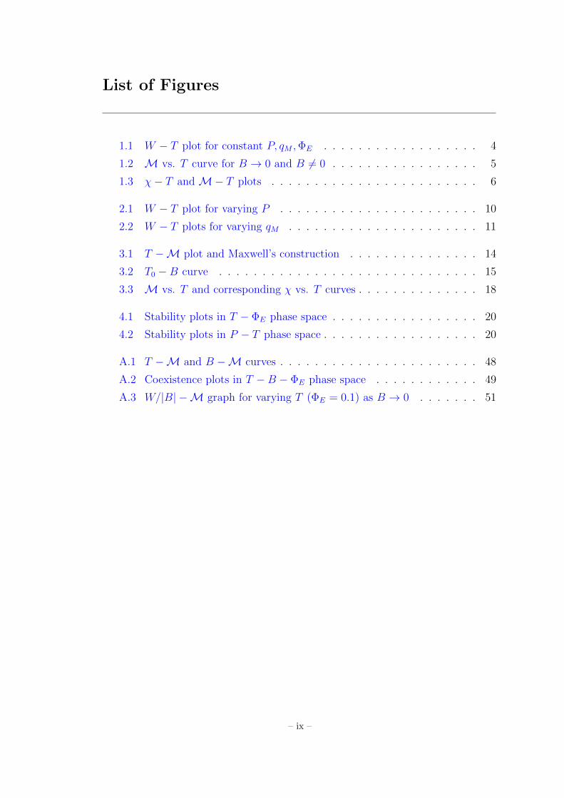
1.1 W − T plot for constant P, qM ,ΦE . . . . . . . . . . . . . . . . . . 4
1.2 M vs. T curve for B → 0 and B 6= 0 . . . . . . . . . . . . . . . . . 5
1.3 χ− T and M− T plots . . . . . . . . . . . . . . . . . . . . . . . . 6
2.1 W − T plot for varying P . . . . . . . . . . . . . . . . . . . . . . . 10
2.2 W − T plots for varying qM . . . . . . . . . . . . . . . . . . . . . . 11
3.1 T −M plot and Maxwell’s construction . . . . . . . . . . . . . . . 14
3.2 T0 −B curve . . . . . . . . . . . . . . . . . . . . . . . . . . . . . . 15
3.3 M vs. T and corresponding χ vs. T curves . . . . . . . . . . . . . . 18
4.1 Stability plots in T − ΦE phase space . . . . . . . . . . . . . . . . . 20
4.2 Stability plots in P − T phase space . . . . . . . . . . . . . . . . . . 20
A.1 T −M and B −M curves . . . . . . . . . . . . . . . . . . . . . . . 48
A.2 Coexistence plots in T −B − ΦE phase space . . . . . . . . . . . . 49
A.3 W/|B| −M graph for varying T (ΦE = 0.1) as B → 0 . . . . . . . 51
– ix –
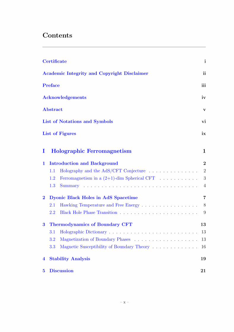
Contents
Certificate i
Academic Integrity and Copyright Disclaimer ii
Preface iii
Acknowledgements iv
Abstract v
List of Notations and Symbols vi
List of Figures ix
I Holographic Ferromagnetism 1
1 Introduction and Background 2
1.1 Holography and the AdS/CFT Conjecture . . . . . . . . . . . . . . 2
1.2 Ferromagnetism in a (2+1)-dim Spherical CFT . . . . . . . . . . . 3
1.3 Summary . . . . . . . . . . . . . . . . . . . . . . . . . . . . . . . . 4
2 Dyonic Black Holes in AdS Spacetime 7
2.1 Hawking Temperature and Free Energy . . . . . . . . . . . . . . . . 8
2.2 Black Hole Phase Transition . . . . . . . . . . . . . . . . . . . . . . 9
3 Thermodynamics of Boundary CFT 13
3.1 Holographic Dictionary . . . . . . . . . . . . . . . . . . . . . . . . . 13
3.2 Magnetization of Boundary Phases . . . . . . . . . . . . . . . . . . 13
3.3 Magnetic Susceptibility of Boundary Theory . . . . . . . . . . . . . 16
4 Stability Analysis 19
5 Discussion 21
– x –
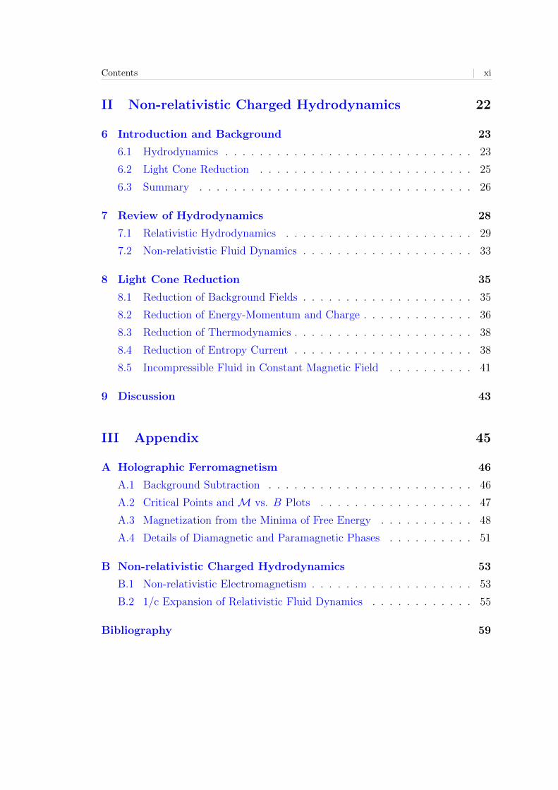
Contents | xi
II Non-relativistic Charged Hydrodynamics 22
6 Introduction and Background 23
6.1 Hydrodynamics . . . . . . . . . . . . . . . . . . . . . . . . . . . . . 23
6.2 Light Cone Reduction . . . . . . . . . . . . . . . . . . . . . . . . . 25
6.3 Summary . . . . . . . . . . . . . . . . . . . . . . . . . . . . . . . . 26
7 Review of Hydrodynamics 28
7.1 Relativistic Hydrodynamics . . . . . . . . . . . . . . . . . . . . . . 29
7.2 Non-relativistic Fluid Dynamics . . . . . . . . . . . . . . . . . . . . 33
8 Light Cone Reduction 35
8.1 Reduction of Background Fields . . . . . . . . . . . . . . . . . . . . 35
8.2 Reduction of Energy-Momentum and Charge . . . . . . . . . . . . . 36
8.3 Reduction of Thermodynamics . . . . . . . . . . . . . . . . . . . . . 38
8.4 Reduction of Entropy Current . . . . . . . . . . . . . . . . . . . . . 38
8.5 Incompressible Fluid in Constant Magnetic Field . . . . . . . . . . 41
9 Discussion 43
III Appendix 45
A Holographic Ferromagnetism 46
A.1 Background Subtraction . . . . . . . . . . . . . . . . . . . . . . . . 46
A.2 Critical Points and M vs. B Plots . . . . . . . . . . . . . . . . . . 47
A.3 Magnetization from the Minima of Free Energy . . . . . . . . . . . 48
A.4 Details of Diamagnetic and Paramagnetic Phases . . . . . . . . . . 51
B Non-relativistic Charged Hydrodynamics 53
B.1 Non-relativistic Electromagnetism . . . . . . . . . . . . . . . . . . . 53
B.2 1/c Expansion of Relativistic Fluid Dynamics . . . . . . . . . . . . 55
Bibliography 59
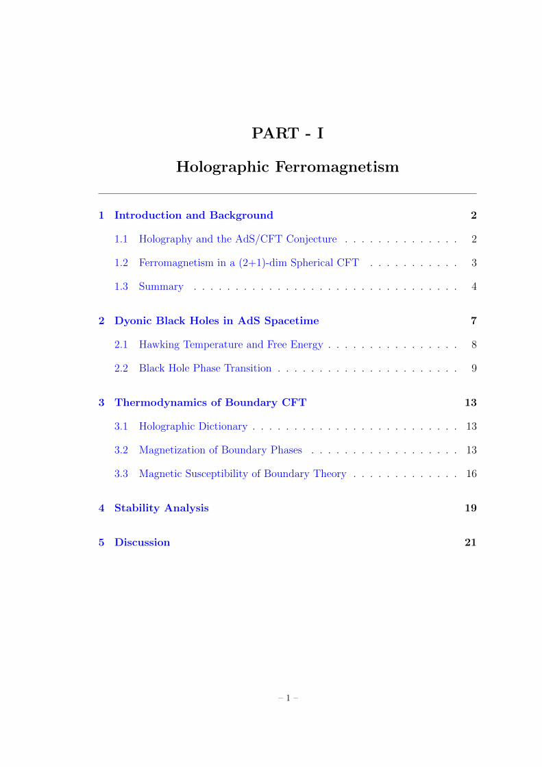
PART - I
Holographic Ferromagnetism
1 Introduction and Background 2
1.1 Holography and the AdS/CFT Conjecture . . . . . . . . . . . . . . 2
1.2 Ferromagnetism in a (2+1)-dim Spherical CFT . . . . . . . . . . . 3
1.3 Summary . . . . . . . . . . . . . . . . . . . . . . . . . . . . . . . . 4
2 Dyonic Black Holes in AdS Spacetime 7
2.1 Hawking Temperature and Free Energy . . . . . . . . . . . . . . . . 8
2.2 Black Hole Phase Transition . . . . . . . . . . . . . . . . . . . . . . 9
3 Thermodynamics of Boundary CFT 13
3.1 Holographic Dictionary . . . . . . . . . . . . . . . . . . . . . . . . . 13
3.2 Magnetization of Boundary Phases . . . . . . . . . . . . . . . . . . 13
3.3 Magnetic Susceptibility of Boundary Theory . . . . . . . . . . . . . 16
4 Stability Analysis 19
5 Discussion 21
– 1 –
1 | Introduction and Background
1.1 Holography and the AdS/CFT Conjecture
Holographic Principle is a conjecture in string theory, which predicts that all the
information of a (d+1)-dimensional gravitational theory, can be encoded in the
(d)-dimensional boundary of the spacetime. The principle was first proposed by
Gerard ’t Hooft, though Leonard Susskind gave it precise string theoretic inter-
pretation combining ideas from ’t Hooft and Charles Thorn.
The idea of holography was inspired from black hole thermodynamics. In the
1970’s, Jacob Bekenstein and Stephen Hawking, among many others, realized that
black holes have rich thermodynamic structure. Precise expressions for various
quantities like entropy, temperature, free energy etc. were given, and were shown
to obey the first law of thermodynamics. As it turns out, entropy of a black hole
is proportional to the area of its horizon and not its volume, which in some sense
is counter intuitive because entropy being an extensive quantity, one would expect
it to be proportional to volume. Since entropy of any thermodynamical object
is equal to the logarithm of total number of underlying quantum micro-states,
it makes us think that all the information (micro-states) of a black hole can be
encoded in a theory living in one lower dimension.
Holographic principle by itself is a very strong statement, which till date does not
have any precise mathematical derivation or experimental proof. However, string
theory provides a canonical example of this holographic principle. The example
is known as the AdS/CFT conjecture, proposed by Juan Maldacena in late 1997
[3, 4]. The conjecture relates two seemingly different theories living in different di-
mensions. The first one is a gravity theory in a (d+1)-dimensional asymptotically
AdS spacetime (a mathematical spacetime with a constant negative cosmological
constant) and the second one is a quantum field theory with conformal invari-
ance1 living on the d dimensional boundary of the AdS spacetime. The conjecture
states that these two theories are dual to each other, i.e. when the field theory
1Conformal Invariance consists of Lorentz Transformations, spacetime translations, Dilatation
and Special Conformal Transformation (SCT).
– 2 –
Chapter 1. Introduction and Background | 3
is in strongly coupled regime the corresponding gravity theory is weakly coupled
and vice-versa. Because of this particular character, the conjecture turns out to
be an essential tool to deal with strongly coupled quantum field theories. The cor-
respondence has also been applied to study hydrodynamic properties (low energy
fluctuations from thermal equilibrium) of different strongly coupled systems. The
first attempt was made by Policastro, Son and Starinets in [5, 6]. They calculated
the shear viscosity to entropy density ratio of a strongly coupled fluid system and
found that it has a universal value. This value was pretty close to the experimen-
tally measured value of shear-viscosity to entropy density ratio of strongly coupled
quark-gluon plasma produced at RHIC (Relativistic Heavy Ion Collider) after the
collision of two heavy ions.
Recently there has been much interest in holographic study of condensed matter
systems. Different properties of (d + 1) dimensional condensed matter systems
(for example super-conductors, Fermi liquid systems and many more [7, 9, 10])
are being studied from the perspective of string theory.
1.2 Ferromagnetism in a (2+1)-dim Spherical CFT
In the current work, we apply the AdS/CFT conjecture to study magnetic prop-
erties of a conformal field theory living on a two-sphere. For that, we consider a
(3 + 1) dimensional dyonic black hole spacetime as our bulk system.
We showed in [1] that when these black holes are considered in an ensemble with
constant magnetic charge (qM) and electric potential at infinity (ΦE), they exhibit
a small-large black hole phase transition. For a particular set of external control
thermodynamic parameters, T , ΦE and qM there exists multiple solutions of black
hole radii (the one with larger radii is termed to be Large Black Hole and one with
smaller as Small Black Hole), and the system chooses the one which has lower free
energy. TheAdS/CFT duality then suggests that the boundary theory, which lives
on the surface of a sphere, should also exhibit some kind of phase transition - which
we found to be a ferromagnetic-kind phase transition. The boundary theory has
zero magnetization at high temperatures, whereas below a transition temperature
(analogue of the Curie’s point) system instantaneously picks a preferred direction,
Chapter 1. Introduction and Background | 4
and has an overall finite but constant magnetization. This should be contrasted
with the ferromagnetism we see in usual materials, where below the curie point,
magnetization continuously increases with the drop in temperature.
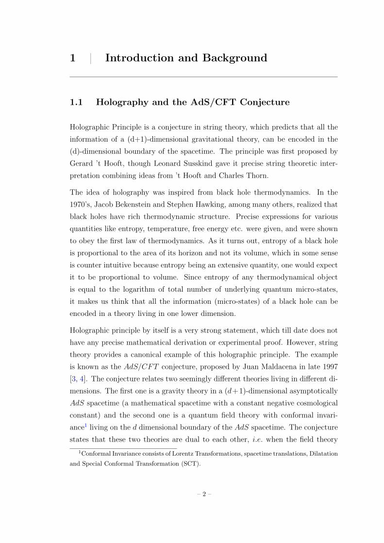
1.3 Summary
We consider a spherical dyonic black hole solution in (3 + 1)-dim asymptotically
AdS spacetime. We calculate free energy (W ) and temperature (T ) of this system.
The self intersection of W − T plot (Fig. 1.1) shows that there exist multiple
phases in the bulk theory, i.e. at a particular temperature, magnetic charge and
electric potential, there exist multiple black hole solutions with different radii and
free energies. The bulk theory exhibits a small-large black hole phase transition
as the temperature crosses the self intersection point, denoted as the coexistence
temperature.
Figure 1.1: W − T plot for all other parameters fixed (P = 0.0035, ΦE = 0.8, qM =
0.068). The graph has three separate branches: Branch-1 (Blue), Branch-2 (Red) and
Branch-3 (Green).
We further study the magnetic properties of a (2+1) dimensional boundary CFT ,
which is dual to our bulk black hole spacetime. The free energy of the CFT is
conjectured to be the free energy of the bulk spacetime by the AdS/CFT conjec-
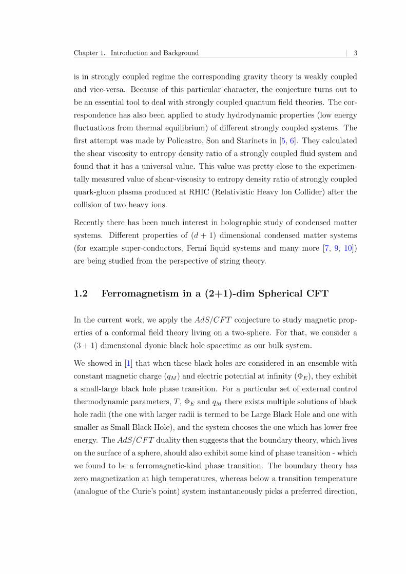
ture. We calculate magnetization of the CFT and find that in B → 0 limit the
boundary theory shows a ferromagnetic like behavior. Above a temperature To
the dominant phase has zero magnetization whereas below To a constant magne-
Chapter 1. Introduction and Background | 5
tization phase is dominant (Fig. 1.2). Unlike a ferromagnetic system though, we
find a discontinuity in magnetization at T0.
Figure 1.2: M vs. T curve for B → 0 (blue curve) and B 6= 0 (red and green curve
for B < 0 and B > 0 respectively). At the transition temperature a sharp jump in
magnetization is observed. Low temperature phase has constant magnetization and
high temperature phase has zero magnetization.
In presence of a finite magnetic field we calculate susceptibility χ of the system
and observe diamagnetic (χ < 0) or paramagnetic (χ > 0) behavior depending on
the temperature and magnetic field. We brief our observations here and present
the details in Section (3):
• There exists a maximum magnetic field B∗ above which the thermodynamics
is dominated by a diamagnetic phase for any temperature. This phase of
CFT is dual to the single black hole phase in the bulk. See Fig. (1.3a).
• For Bc < B < B∗ (Bc is the critical magnetic field), the thermodynamics
is again governed by a single phase (which is dual to the single black hole
phase in bulk). But this phase shows two crossovers between diamagnetic
and paramagnetic phases. Very high and very low temperature phases are
diamagnetic, while in between the system is paramagnetic. See Fig. (1.3b).
• Criticality appears at B = Bc. Two new phases nucleate (one of which is
thermodynamically unstable). Other two stable phases are dual to small
and large black holes in bulk. If B is sufficiently smaller than Bc, we see
a transition between a paramagnetic (dual to SBH) phase and diamagnetic
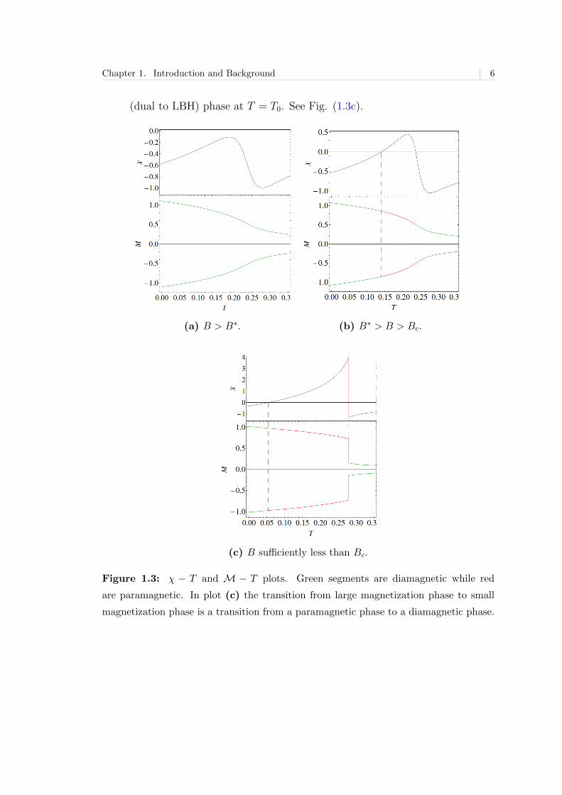
Chapter 1. Introduction and Background | 6
(dual to LBH) phase at T = T0. See Fig. (1.3c).
(a) B > B∗. (b) B∗ > B > Bc.
(c) B sufficiently less than Bc.
Figure 1.3: χ − T and M − T plots. Green segments are diamagnetic while red
are paramagnetic. In plot (c) the transition from large magnetization phase to small
magnetization phase is a transition from a paramagnetic phase to a diamagnetic phase.
2 | Dyonic Black Holes in AdS Spacetime
AdS spacetime is the vacuum solution of Einstein’s equations in presence of a
negative cosmological constant (Λ), much like Minkowski spacetime is the solution
without any Λ. Similar to the Minkowski case [18], we can have a maximally
symmetric solution to the Einstein’s equations, which will give us a black hole in
asymptotically AdS space.
We consider the Reissner-Nordstrom action in four dimensions in presence of a
cosmological term, which describes our system of interest:
I =1
16πG4
∫d4x√g
(−R + F 2 − 6
b2
). (2.1)
Variation of this action gives the equations of motion:
Rµν −1
2gµνR−
3
b2gµν = 2(FµλF
λν −
1
4gµνFαβF
αβ), ∇µFµν = 0, (2.2)
maximally symmetric solution to which is given by:
A =
(−qEr
+qEr+
)dt+ (qM cos θ) dφ, (2.3)
ds2 = −f(r)dt2 +1
f(r)dr2 + r2dθ2 + r2sin2θdφ2, (2.4)
where, Aµ is the U(1) gauge field and
f(r) =
(1 +
r2
b2− 2M
r+q2E + q2M
r2
). (2.5)
qE, qM and M are integration constants, identified as electric charge, magnetic
charge and mass of the black hole respectively. r+, the horizon of the black hole
is given by the solution of:
f(r+) =
(1 +
r2+b2− 2M
r++q2E + q2Mr2+
)= 0. (2.6)
Subsequently we aim at studying the thermodynamics of the black hole system,
for which we choose an ensemble where qM and the asymptotic value of At is
constant, which implies that the electric potential ΦE, defined as:
ΦE =qEr+, (2.7)
is constant in our thermodynamic analysis.
– 7 –
Chapter 2. Dyonic Black Holes in AdS Spacetime | 8
2.1 Hawking Temperature and Free Energy
To study thermodynamic description of a system, one needs the equation of state
along with the expression for free energy specific to the ensemble under consider-
ation. In black hole systems, a generic procedure has been prescribed by Gibbons
and Hawking in Euclidean framework, to get temperature and free energy.
We define the euclidean time τ = ιt, which can be shown to be S1 angular coor-
dinate after appropriate coordinate transformations [19]. In the Euclidean frame-
work we can define the partition function of the system as:
Z =
∫[Dg]e−IE , (2.8)
where IE is the Euclidean action. In the semi-classical limit that we are consider-
ing, the dominant contribution to the path integral comes from classical solutions
to the equations of motion. In this case,
logZ = −IonshellE , (2.9)
where IonshellE is the action evaluated on equations of motion. Using Eqn. (2.2) we
can write
IonshellE =1
16πG4
∫d4x√g
(F 2 +
6
b2
). (2.10)
Free energy is thus given by:
W = − 1
βlnZ =
Ionshellβ
. (2.11)
The on-shell action is divergent because the r integration ranges from r+ to ∞.
Therefore, we need to regularize the action by introducing a finite cutoff R. Then,
to renormalize the action, we can either add some counter-term to the original
action or we can subtract the contribution of a background spacetime. Here we
follow the first prescription. Method of background subtraction is discussed in
Appendix (A.1).
For an electromagnetically charged black hole with mass M , magnetic charge
qM and electric potential at infinity ΦE, the regularised on-shell action is given
Chapter 2. Dyonic Black Holes in AdS Spacetime | 9
by
IBH =1
16πG4
∫ R
r+
d4x√g
(F 2 +
6
b2
)=
β
4G4
[2(Φ2
Er2+ − q2M)
R+
6R3
3b2−
2(Φ2Er
2+ − q2M)
r+−
6r3+3b2
]. (2.12)
Here R is the cutoff. We shall take R→∞ at the end. β is the period of Euclidean
time coordinate τ , identified as inverse Hawking temperature
T =1
β=f ′(r+)
4π=
1
4πr+
[1 +
3r2+b2− Φ2
E −q2Mr2+
]. (2.13)
This equation serves as the equation of state of the black hole.
Note that the second term in equation (2.12) gives a diverging contribution to
free energy as R → ∞. To tame the divergence we add counterterms follow-
ing [12]. We find that the on-shell action can be made finite with the following
counterterms,
Sct =1
8πG4
∫∂M
d3x√−γ(c1 + c2R
(3)). (2.14)
Here ∂M is the asymptotic boundary of AdS spacetime, γ is the induced metric
on the boundary, R(3) is the Ricci scalar calculated for the metric γ. c1 and c2 are
two numerical constants, their values are given by
c1 = −1
b, c2 =
b
4. (2.15)
Hence, the free energy is given by,
W =I
β=
r+4G4
[1−
r2+b2− Φ2
E +3q2Mr2+
]. (2.16)
r+ in the above equation just serves as a parameter, and is to be replaced using
Eqn. (2.13) for all purposes. Therefore in our ensemble W is to be understood as
W (T,ΦE, qM).
2.2 Black Hole Phase Transition
We now plot W (T,ΦE, qM) with respect to T for everything else held fixed. We
find that for a particular temperature, there exists multiple solutions of the black
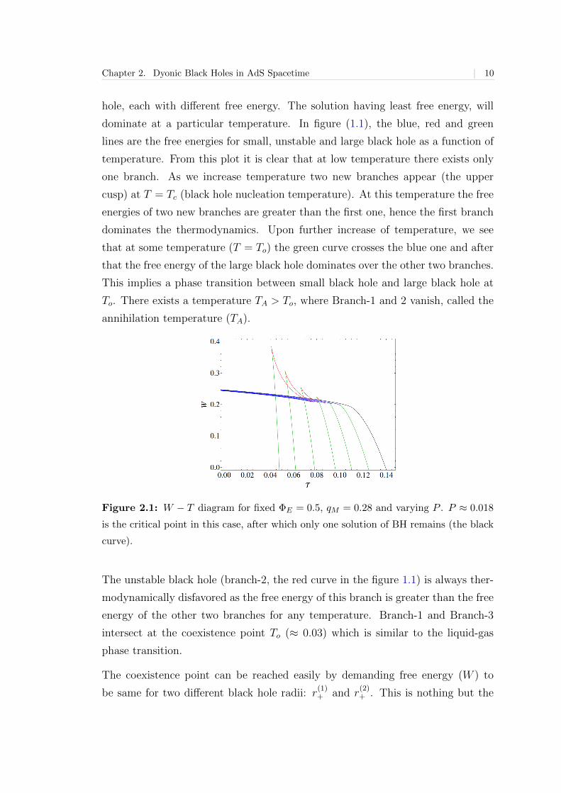
Chapter 2. Dyonic Black Holes in AdS Spacetime | 10
hole, each with different free energy. The solution having least free energy, will
dominate at a particular temperature. In figure (1.1), the blue, red and green
lines are the free energies for small, unstable and large black hole as a function of
temperature. From this plot it is clear that at low temperature there exists only
one branch. As we increase temperature two new branches appear (the upper
cusp) at T = Tc (black hole nucleation temperature). At this temperature the free
energies of two new branches are greater than the first one, hence the first branch
dominates the thermodynamics. Upon further increase of temperature, we see
that at some temperature (T = To) the green curve crosses the blue one and after
that the free energy of the large black hole dominates over the other two branches.
This implies a phase transition between small black hole and large black hole at
To. There exists a temperature TA > To, where Branch-1 and 2 vanish, called the
annihilation temperature (TA).
Figure 2.1: W − T diagram for fixed ΦE = 0.5, qM = 0.28 and varying P . P ≈ 0.018
is the critical point in this case, after which only one solution of BH remains (the black
curve).
The unstable black hole (branch-2, the red curve in the figure 1.1) is always ther-
modynamically disfavored as the free energy of this branch is greater than the free
energy of the other two branches for any temperature. Branch-1 and Branch-3
intersect at the coexistence point To (≈ 0.03) which is similar to the liquid-gas
phase transition.
The coexistence point can be reached easily by demanding free energy (W ) to
be same for two different black hole radii: r(1)+ and r
(2)+ . This is nothing but the
Chapter 2. Dyonic Black Holes in AdS Spacetime | 11
Maxwell’s construction. As we vary the temperature, black hole never goes to
Branch-2 phase, but jumps from Branch-1 to Branch-3 directly at the coexistence
point.
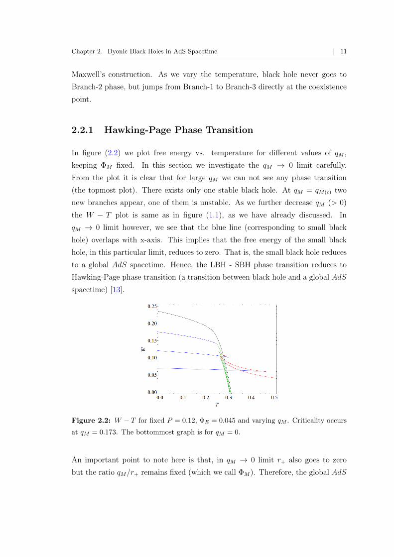
2.2.1 Hawking-Page Phase Transition
In figure (2.2) we plot free energy vs. temperature for different values of qM ,
keeping ΦM fixed. In this section we investigate the qM → 0 limit carefully.
From the plot it is clear that for large qM we can not see any phase transition
(the topmost plot). There exists only one stable black hole. At qM = qM(c) two
new branches appear, one of them is unstable. As we further decrease qM (> 0)
the W − T plot is same as in figure (1.1), as we have already discussed. In
qM → 0 limit however, we see that the blue line (corresponding to small black
hole) overlaps with x-axis. This implies that the free energy of the small black
hole, in this particular limit, reduces to zero. That is, the small black hole reduces
to a global AdS spacetime. Hence, the LBH - SBH phase transition reduces to
Hawking-Page phase transition (a transition between black hole and a global AdS
spacetime) [13].
Figure 2.2: W − T for fixed P = 0.12, ΦE = 0.045 and varying qM . Criticality occurs
at qM = 0.173. The bottommost graph is for qM = 0.
An important point to note here is that, in qM → 0 limit r+ also goes to zero
but the ratio qM/r+ remains fixed (which we call ΦM). Therefore, the global AdS
Chapter 2. Dyonic Black Holes in AdS Spacetime | 12
spacetime has a constant ΦM . Since we are working in a constant ΦE ensemble,
the global AdS space has a constant electric potential as well.
3 | Thermodynamics of Boundary CFT
(3 + 1)-dim spherical dyonic black hole in asymptotically AdS spacetime is con-
jectured to be dual to a (2 + 1)-dim CFT living on the boundary of the AdS
space, which has topology R×S2. In this section we will study the implication of
small-large black hole phase transition of the bulk on the boundary theory.
3.1 Holographic Dictionary
The bulk gauge field is dual to a global U(1) current operator Jµ. The CFT has
a conserved global charge 〈J t〉 given by⟨J t⟩
=qE
16πG4
=
√2N3/2qE24πb2
(3.1)
where, we use the holographic dictionary
1
16πG4
=
√2N3/2
24πb2, N is the degree of the gauge group of the CFT .
The boundary CFT also has a constant magnetic field. The strength of the mag-
netic field is given by B = qM/b2 which can be read off from the asymptotic value
of bulk field strength obtained from equation (2.3). We shall study the magnetic
properties of this strongly coupled system using the holographic setup.
In Section (3.2), we see that the CFT undergoes a phase transition. A system in
finite volume, in general, does not exhibit any phase transition. But in the large
N limit, i.e., when the number of degrees of freedom goes to infinity, it is possible
to have a phase transition even in finite volume.
3.2 Magnetization of Boundary Phases
The magnetic field in our boundary theory is given by,
B =qMb2. (3.2)
When we consider thermodynamics of the boundary theory we define a variable
M (magnetization), conjugate to the external magnetic field B. Different phases
– 13 –
Chapter 3. Thermodynamics of Boundary CFT | 14
of boundary theory are also characterized by this new variable M defined by the
following relation using Eqn. (2.16),
M = −∂W∂B
∣∣∣∣T
= −b2(qMr+
). (3.3)
It is worth to note that the positive definiteness of r+ implies M and B always
have opposite sign.
We calculate free energy and temperature of the CFT in terms of B and M(boundary parameters) to study the phase structure of the system,
W =1
4
[−(1− Φ2
E)b4B
M− 3BM+ b10
B3
M3
], (3.4)
T =1
β=
1
4π
[−(1− Φ2
E)1
b4MB− 3b2
B
M+
1
b8M3
B
]. (3.5)
W in equation (3.4) can be plotted against T for varying B. Since B is proportional
to qM , the plot is the same as in figure (2.2). For B above a critical value Bc
(which is proportional to qM(c), discussed in Section 2.2.1) there exists only one
phase of boundary CFT and magnetization of this phase is a continuous function
of temperature. As B goes below Bc the boundary theory develops two more new
phases. Therefore, in this case the theory has three different phases (in a given
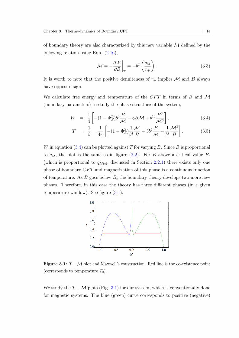
temperature window). See figure (3.1).
Figure 3.1: T −M plot and Maxwell’s construction. Red line is the co-existence point
(corresponds to temperature T0).
We study the T −M plots (Fig. 3.1) for our system, which is conventionally done
for magnetic systems. The blue (green) curve corresponds to positive (negative)
Chapter 3. Thermodynamics of Boundary CFT | 15
magnetic field. In this figure we see that, below a critical temperature there exists
only one phase with high magnetization (dual to small black hole). Above the
critical temperature, there are three possible phases with different magnetization.
Among them the middle one is thermodynamically unstable. The phase with
small magnetization corresponds to the large black hole phase in the dual theory.
The red line indicates the transition temperature To. Above this temperature,
thermodynamics is dominated by the phase with small magnetization. Therefore
a sharp jump in magnetization is observed at the transition temperature. In
figure (1.2) we plot the same graph removing the unstable branch using Maxwell’s
construction. M vs. T plots for different values of magnetic field and B vs. Mplots for different values of temperature are discussed in Appendix (A.2).
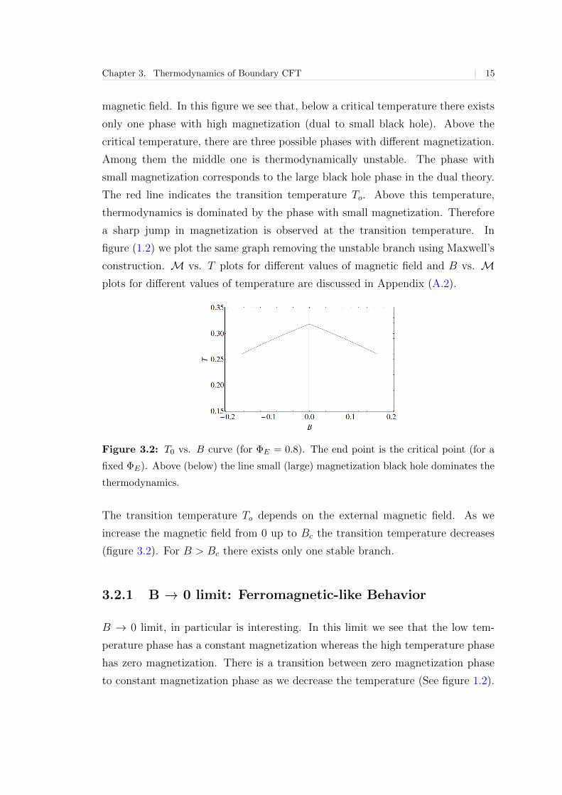
Figure 3.2: T0 vs. B curve (for ΦE = 0.8). The end point is the critical point (for a
fixed ΦE). Above (below) the line small (large) magnetization black hole dominates the
thermodynamics.
The transition temperature To depends on the external magnetic field. As we
increase the magnetic field from 0 up to Bc the transition temperature decreases
(figure 3.2). For B > Bc there exists only one stable branch.
3.2.1 B → 0 limit: Ferromagnetic-like Behavior
B → 0 limit, in particular is interesting. In this limit we see that the low tem-
perature phase has a constant magnetization whereas the high temperature phase
has zero magnetization. There is a transition between zero magnetization phase
to constant magnetization phase as we decrease the temperature (See figure 1.2).
Chapter 3. Thermodynamics of Boundary CFT | 16
Unlike ferromagnetic materials, here we find that the magnetization is discontin-
uous at the transition temperature. The constant magnetization phase is dual
to global AdS phase in the bulk. As we have discussed before, in this limit the
radius of small black hole goes to zero with qM/r+ fixed. In other words the small
black hole evaporates to global AdS with constant ΦE and M. A more detailed
discussion can be found in Appendix (A.3).
As we have explained before, in the limit B → 0, LBH/SBH phase transition re-
duces to Hawking-Page phase transition. Therefore, low temperature phase (dual
to global AdS) of the boundary theory has zero free energy whereas the high tem-
perature phase dual to LBH has free energy of order N3/2 in the limit N → ∞.
This phase transition is identified with confinement-deconfinement phase transi-
tion of gauge theory [14]. Therefore, we see that the confined phase has a constant
magnetization whereas the deconfined phase has zero magnetization.
3.3 Magnetic Susceptibility of Boundary Theory
Depending on the temperature and applied magnetic field, boundary theory shows
either diamagnetic or paramagnetic behavior. To study the same we calculate
magnetic susceptibility using the formula:
χ =∂M∂B
∣∣∣∣T
. (3.6)
A system is said to be diamagnetic if χ < 0 and paramagnetic if χ > 0. The
magnetic properties of a physical substance mainly depend on the electrons in the
substance. The electrons are either free or bound to atoms. When we apply an
external magnetic field these electrons react against that field. In general one can
see two important effects. One, the electrons start moving in a quantised orbit
in presence of the magnetic field. Two, the spins of the electrons tend to align
parallel to the magnetic field. One can neglect the effect of atomic nuclei compared
to these two effects, as they are much heavier than electrons. The orbital motion
of electrons is responsible for diamagnetism whereas, alignment of electrons’ spin
along the magnetic field gives rise to paramagnetism. In a physical substance,
these two effects compete. In diamagnetic material the first one (orbital motion)
is stronger than the second one, and vice-versa in a paramagnetic material.
Chapter 3. Thermodynamics of Boundary CFT | 17
The temperature in (equation 3.5) can be written in the following differential form
for a constant ΦE:
dT =∂T
∂BdB +
∂T
∂MdM. (3.7)
χ from this expression can be written as
χ =dMdB
∣∣∣∣T
=∂T
∂B
∂M∂T
=MB
(3b10B2 +M4 − b4M2 (1− Φ2
E)
3b10B2 + 3M4 − b4M2 (1− Φ2E)
). (3.8)
We plot χ against T for various B to study the magnetic behaviour of the system.
Our results are as follows:
1. There exists a magnetic field B∗ > Bc, above which the CFT is diamagnetic
for all temperatures (see figure 1.3a).
2. For Bc < B < B∗, still the boundary theory has a single phase but this
phase shows two crossovers between paramagnetic and diamagnetic phases.
At high and low temperature the system behaves like a diamagnetic system,
while in between it shows paramagnetic behavior. See figure (1.3b).
3. For B < Bc (but still close to Bc), the unstable branch of BH pops up. Thus
we see a phase transition at To from Small BH branch to Large BH branch,
both of them being paramagnetic. As temperature is decreased (increased),
Small BH (Large BH) branch crosses over to a diamagnetic phase. Figure
(3.3) shows the segment of the curves near T = To.
4. Below Bc, when magnetic field is even below a certain value B# (discussed
in Appendix A.4), the paramagnetic branch of Large BH gets cut off in the
Maxwells’ construction (figure 1.3c). Thus the phase transition occurs from
paramagnetic Small BH to diamagnetic Large BH.
3.3.1 High Temperature Behavior of Magnetic Suscepti-
bility
In the high temperature limit, as we know that only the small magnetization
solution (Large BH) dominates, temperature (equation 3.5) has the leading con-
tribution from:
T ≈ − 3B
4πM(3.9)
Chapter 3. Thermodynamics of Boundary CFT | 18
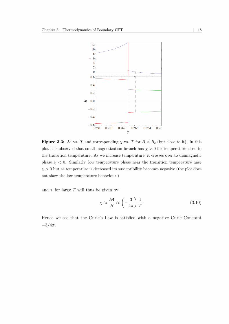
Figure 3.3: M vs. T and corresponding χ vs. T for B < Bc (but close to it). In this
plot it is observed that small magnetization branch has χ > 0 for temperature close to
the transition temperature. As we increase temperature, it crosses over to diamagnetic
phase χ < 0. Similarly, low temperature phase near the transition temperature hase
χ > 0 but as temperature is decreased its susceptibility becomes negative (the plot does
not show the low temperature behaviour.)
and χ for large T will thus be given by:
χ ≈ MB≈(− 3
4π
)1
T. (3.10)
Hence we see that the Curie’s Law is satisfied with a negative Curie Constant
−3/4π.
4 | Stability Analysis
We conclude our discussion by analysing the stability of black hole solutions. When
entropy S is a smooth function of extensive variables xi’s then sub-additivity of
entropy is equivalent to the Hessian matrix[
∂2S∂xi∂xj
]being negative definite. For
canonical ensemble the only extensive variable is mass (or energy), therefore, sub-
additivity of entropy implies that CP > 0. For grand canonical ensemble, the
variables are mass and charges therefore the stability lines are determined by
finding the zeroes of the determinant of the Hessian matrix. It has been argued
in [15] that the zeroes of the determinant of the Hessian of S with respect to M
and qi’s coincide with the zeroes of the determinant of the Hessian of the Gibbs
(Euclidean) action,
IG = β
(M −
∑i
qphysi Φi
)− S (4.1)
with respect to r+ and qi’s keeping β and Φi’s fixed. Note that qi’s are the
charge parameters entering into the black hole solutions where qphysi ’s are the
physical charges. Though this criteria can figure out the instability line in the
phase diagram but it is unable to tell which sides of the phase transition lines
correspond to local stability. One can figure out the stability region by using
the fact that zero chemical potential and high temperature must correspond to a
stable black hole solution.
We compute the zeroes of the Hessian of free energy W = M − ΦEqE − TS with
respect to qE and r+ keeping T and ΦE fixed, which gives us one condition (or
bound) on the phase space. Positivity of temperature will give another condition.
These two conditions give the following bound on the phase space.
3q2M +3r4+b2− r2+(1− Φ2
E) > 0, −q2M +3r4+b2
+ r2+(1− Φ2E) > 0. (4.2)
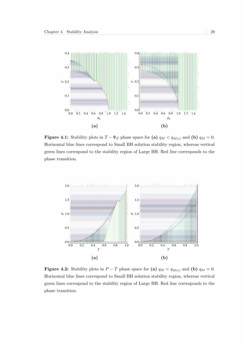
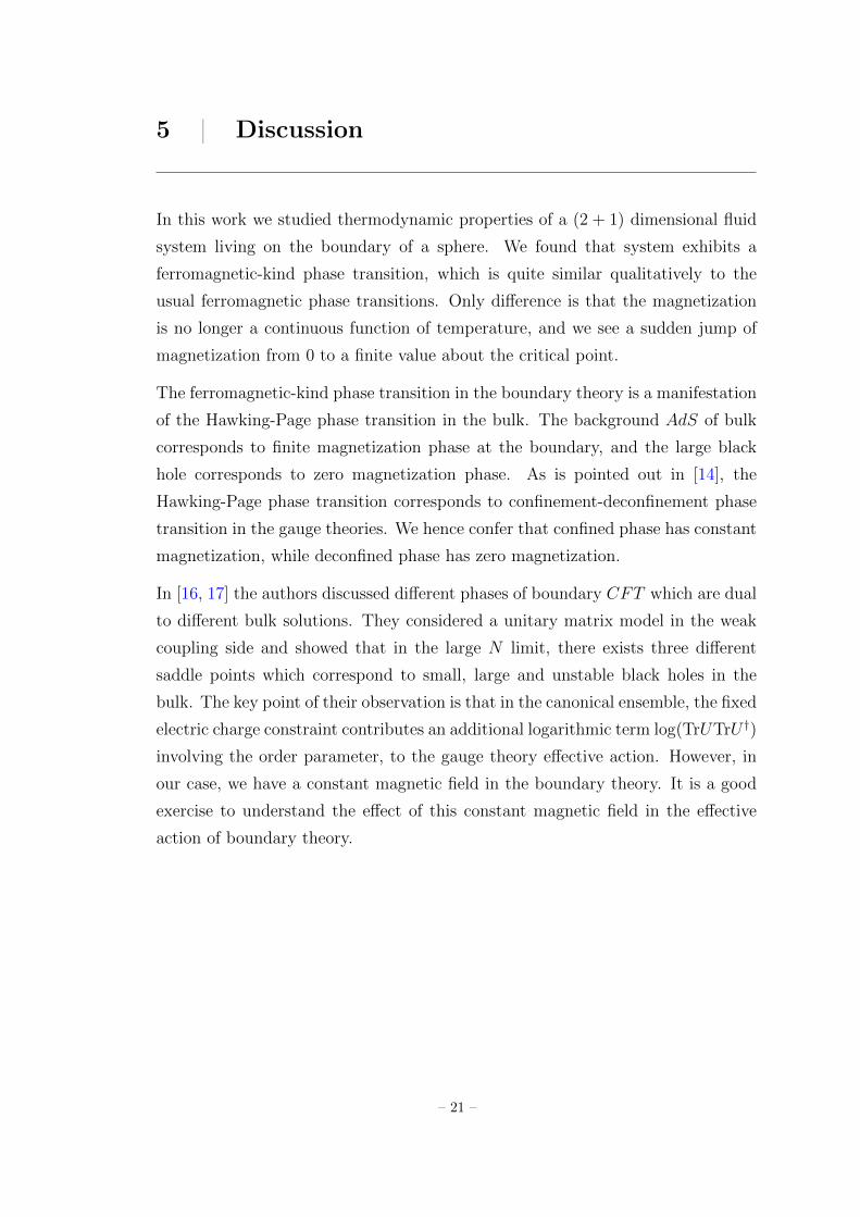
In figure (4.1) and (4.2) We plot these stability lines and find that all values of
qM , ΦE and T > 0 results in a stable solution.
– 19 –
Chapter 4. Stability Analysis | 20
(a) (b)
Figure 4.1: Stability plots in T −ΦE phase space for (a) qM < qM(c) and (b) qM = 0.
Horizontal blue lines correspond to Small BH solution stability region, whereas vertical
green lines correspond to the stability region of Large BH. Red line corresponds to the
phase transition.
(a) (b)
Figure 4.2: Stability plots in P − T phase space for (a) qM < qM(c) and (b) qM = 0.
Horizontal blue lines correspond to Small BH solution stability region, whereas vertical
green lines correspond to the stability region of Large BH. Red line corresponds to the
phase transition.
5 | Discussion
In this work we studied thermodynamic properties of a (2 + 1) dimensional fluid
system living on the boundary of a sphere. We found that system exhibits a
ferromagnetic-kind phase transition, which is quite similar qualitatively to the
usual ferromagnetic phase transitions. Only difference is that the magnetization
is no longer a continuous function of temperature, and we see a sudden jump of
magnetization from 0 to a finite value about the critical point.
The ferromagnetic-kind phase transition in the boundary theory is a manifestation
of the Hawking-Page phase transition in the bulk. The background AdS of bulk
corresponds to finite magnetization phase at the boundary, and the large black
hole corresponds to zero magnetization phase. As is pointed out in [14], the
Hawking-Page phase transition corresponds to confinement-deconfinement phase
transition in the gauge theories. We hence confer that confined phase has constant
magnetization, while deconfined phase has zero magnetization.
In [16, 17] the authors discussed different phases of boundary CFT which are dual
to different bulk solutions. They considered a unitary matrix model in the weak
coupling side and showed that in the large N limit, there exists three different
saddle points which correspond to small, large and unstable black holes in the
bulk. The key point of their observation is that in the canonical ensemble, the fixed
electric charge constraint contributes an additional logarithmic term log(TrUTrU †)
involving the order parameter, to the gauge theory effective action. However, in
our case, we have a constant magnetic field in the boundary theory. It is a good
exercise to understand the effect of this constant magnetic field in the effective
action of boundary theory.
– 21 –
PART - II
Non-relativistic Charged Hydrodynamics
6 Introduction and Background 23
6.1 Hydrodynamics . . . . . . . . . . . . . . . . . . . . . . . . . . . . . 23
6.2 Light Cone Reduction . . . . . . . . . . . . . . . . . . . . . . . . . 25
6.3 Summary . . . . . . . . . . . . . . . . . . . . . . . . . . . . . . . . 26
7 Review of Hydrodynamics 28
7.1 Relativistic Hydrodynamics . . . . . . . . . . . . . . . . . . . . . . 29
7.2 Non-relativistic Fluid Dynamics . . . . . . . . . . . . . . . . . . . . 33
8 Light Cone Reduction 35
8.1 Reduction of Background Fields . . . . . . . . . . . . . . . . . . . . 35
8.2 Reduction of Energy-Momentum and Charge . . . . . . . . . . . . . 36
8.3 Reduction of Thermodynamics . . . . . . . . . . . . . . . . . . . . . 38
8.4 Reduction of Entropy Current . . . . . . . . . . . . . . . . . . . . . 38
8.5 Incompressible Fluid in Constant Magnetic Field . . . . . . . . . . 41
9 Discussion 43
– 22 –
6 | Introduction and Background
6.1 Hydrodynamics
Hydrodynamics is an effective description of nearly equilibrium interacting many
body systems. Fluid systems are considered to be continuous, i.e. when we talk
about an infinitesimal volume element (or ‘fluid particle’), it still contains a large
number of molecules. More specifically, the size of a fluid particle is much much
greater than the mean free path of the system. In the same spirit, velocity of the
fluid at a point is to be considered as the velocity of the respective fluid particle,
and not the velocities of molecules themselves.
A fluid is completely determined by its velocity ~v(~x, t) and the set of independent
thermodynamic parameters (like pressure p(~x, t), energy density ε(~x, t), temper-
ature τ(~x, t), mass density ρ(~x, t), charge density q(~x, t) etc., out of which not
all are independent due to thermodynamic relations and equation of state) as a
function of space and time. The flow of a fluid is governed by a set of equations
known as constitutive equations, which are essentially the conservation equations
for mass, energy, momentum and charge.
The equations of hydrodynamics assume that the fluid is in local thermodynamic
equilibrium at each point in space and time, even though different thermodynamic
quantities may vary. Therefore fluid mechanics essentially applies only when the
length scales of variation of thermodynamic variables are large compared to equi-
libration length scale of the fluid, namely mean free path [20].
Since fluids are not in ‘absolute’ thermodynamic equilibrium, second law of ther-
modynamics tells us that there should not be any local loss of entropy. The
increase of entropy at every spacetime point is called internal friction, viscosity
or dissipation. The dissipation arises due to gradient of thermodynamic quan-
tities in the fluid which takes it away from the equilibrium, and hence is ac-
counted for in the constitutive equations by means of derivative dependence of
mass/energy/momentum/charge flow on fluid variables. However, since the fluid
is assumed to be in local equilibrium, the derivatives are fairly small, and one can
perform a derivative expansion of the theory, to study it order by order in deriva-
– 23 –
Chapter 6. Introduction and Background | 24
tives. The zeroeth order fluid is called the ‘ideal fluid’, i.e. a fluid without any
dissipation. We consider in this work a fluid in first order derivative expansion.
The coefficients coupling to various derivative terms in constitutive equations are
called transport coefficients - they describe the strength of effect of fluctuations of
a thermodynamic parameter on the respective equations. These transport coeffi-
cients can in general be a function of the fluid’s thermodynamic parameters but
not velocity.
As it turns out, not all derivative terms produce entropy; instead some end up
reducing it. Therefore one must explicitly look at the entropy current, to find out
what derivative terms are allowed in the constitutive equations and under what
conditions. Equivalently, entropy current positivity imposes certain constraints on
the transport coefficients of the fluid, while certain transport coefficients are turned
off. The same has been established for uncharged fluids in Landau’s book [20].
One of the goals of this work is to write a consistent entropy current for charged
non-relativistic fluids and get constraints on various transport coefficients.
Landau, in his book on fluid dynamics [20] gives a thorough discussion on un-
charged, non-relativistic as well as relativistic fluids upto first derivative order. In
subsequent years, the charged fluids has been also fairly curated and understood.
In Section (7) we will review the key features of relativistic and non-relativistic
fluid dynamics.
A relativistic fluid theory can obviously be reduced to a non-relativistic theory
under the special case of v c or c → ∞, under certain assumptions1. For
charged fluids this limit has been well studied in [26], and we review its basic
layout in Appendix (B.2). It is shown in [27] however, that one can also reach
to a (d+ 1)-dim non-relativistic fluid theory starting from (d+ 2)-dim relativistic
theory by following a mechanism known as Light Cone Reduction (LCR). We shall
discuss more about Light Cone Reduction in the next section. One of the aims
of this work is to construct a consistent non-relativistic fluid description using
LCR, and compare it to the description already obtained by non-relativistic limit
in [26].
1The assumption involved is that the two limits - non-relativistic limit and continuity limit
of fluids, commute, which as of yet has no underlying reasons to be true.
Chapter 6. Introduction and Background | 25
6.2 Light Cone Reduction
Discrete Light Cone Quantization is a well established mechanism in Quantum
Field Theories, which connects a (d + 2)-dim relativistic theory to a (d + 1)-dim
non-relativistic theory. The mechanism involves a coordinate transformation in
relativistic theory from the Minkowski coordinates xµµ=0,1,..,d+1 to the light cone
coordinates x±, xii=1,2..,d:
x± =1√2
(x0 ± xd+1
). (6.1)
We now let the theory evolve in x+ direction and identify it with the new ‘time’
coordinate (t) of the non-relativistic theory, keeping the x− coordinate fixed (i.e.
∂− acting on any parameter of the theory will vanish). Under this identification
the new theory in (d + 1)-dim with coordinates t, xii=1,2..,d respects the non-
relativistic symmetry [24]. The reduction essentially means that the underlying
symmetry group of relativistic theory (eg. Poincare or Conformal) reduces to
the underlying symmetry group of the non-relativistic theory (eg. Galilean or
Schrodinger respectively).
In some sense, this way of looking at a non-relativistic theories is much more
proper, because the ‘Galilean Invariance’ is fundamental backbone of a non-relativistic
system. On the other hand however, the small velocity limit of a relativistic theory
is bound to give a non-relativistic theory, but there is no unique and consistent
way to do it. Especially in fluids, we have an underlying caveat that the two limits:
hydrodynamic and non-relativistic, might not commute.
In the current work we perform LCR on a (d + 2)-dim relativistic hydrodynamic
theory, and obtain a (d+1)-dim non-relativistic theory. It has been already shown
in [25] that this gives a consistent non-relativistic fluid in uncharged case, except
that the extensivity is lost during reduction. Here we extend this idea to charged
non-relativistic fluids as well. We discuss more about this issue in Section (8).
Authors in [26] already studied such fluids via a 1/c expansion; we will discuss
disparities in their and our results and reasons for them to arise.
Chapter 6. Introduction and Background | 26
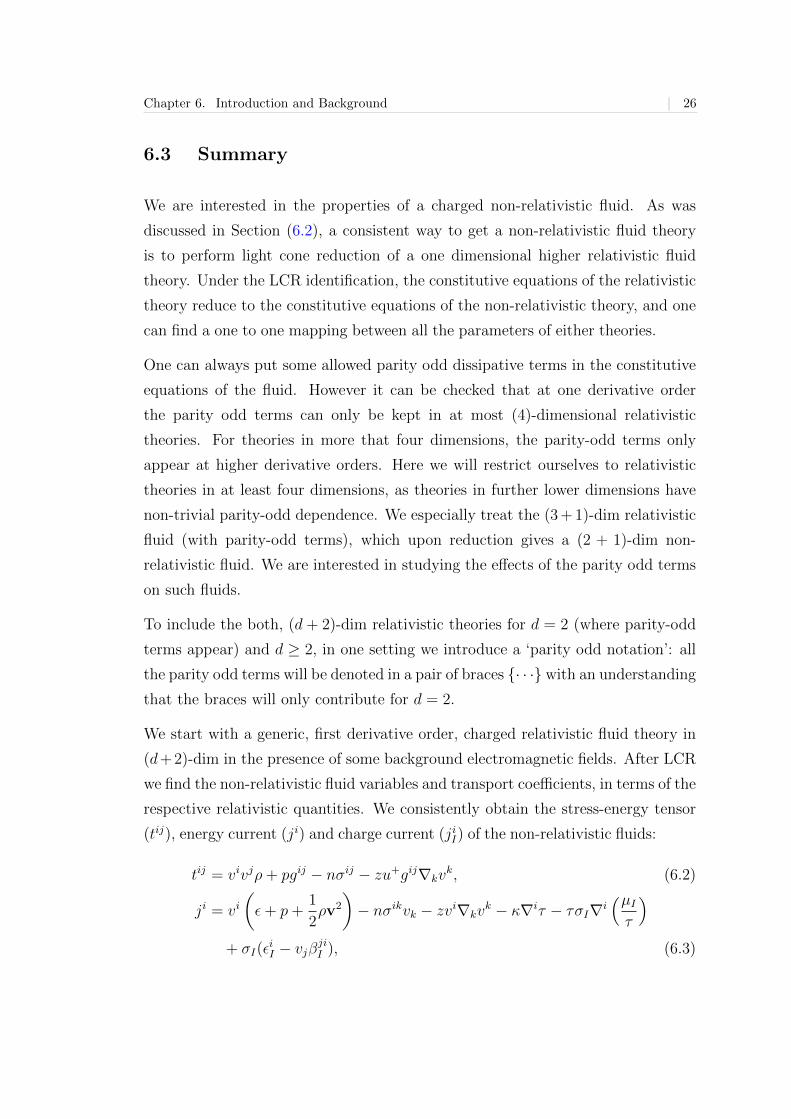
6.3 Summary
We are interested in the properties of a charged non-relativistic fluid. As was
discussed in Section (6.2), a consistent way to get a non-relativistic fluid theory
is to perform light cone reduction of a one dimensional higher relativistic fluid
theory. Under the LCR identification, the constitutive equations of the relativistic
theory reduce to the constitutive equations of the non-relativistic theory, and one
can find a one to one mapping between all the parameters of either theories.
One can always put some allowed parity odd dissipative terms in the constitutive
equations of the fluid. However it can be checked that at one derivative order
the parity odd terms can only be kept in at most (4)-dimensional relativistic
theories. For theories in more that four dimensions, the parity-odd terms only
appear at higher derivative orders. Here we will restrict ourselves to relativistic
theories in at least four dimensions, as theories in further lower dimensions have
non-trivial parity-odd dependence. We especially treat the (3 + 1)-dim relativistic
fluid (with parity-odd terms), which upon reduction gives a (2 + 1)-dim non-
relativistic fluid. We are interested in studying the effects of the parity odd terms
on such fluids.
To include the both, (d + 2)-dim relativistic theories for d = 2 (where parity-odd
terms appear) and d ≥ 2, in one setting we introduce a ‘parity odd notation’: all
the parity odd terms will be denoted in a pair of braces · · · with an understanding
that the braces will only contribute for d = 2.
We start with a generic, first derivative order, charged relativistic fluid theory in
(d+2)-dim in the presence of some background electromagnetic fields. After LCR
we find the non-relativistic fluid variables and transport coefficients, in terms of the
respective relativistic quantities. We consistently obtain the stress-energy tensor
(tij), energy current (ji) and charge current (jiI) of the non-relativistic fluids:
tij = vivjρ+ pgij − nσij − zu+gij∇kvk, (6.2)
ji = vi(ε+ p+
1
2ρv2
)− nσikvk − zvi∇kv
k − κ∇iτ − τσI∇i(µIτ
)+ σI(ε
iI − vjβ
jiI ), (6.3)
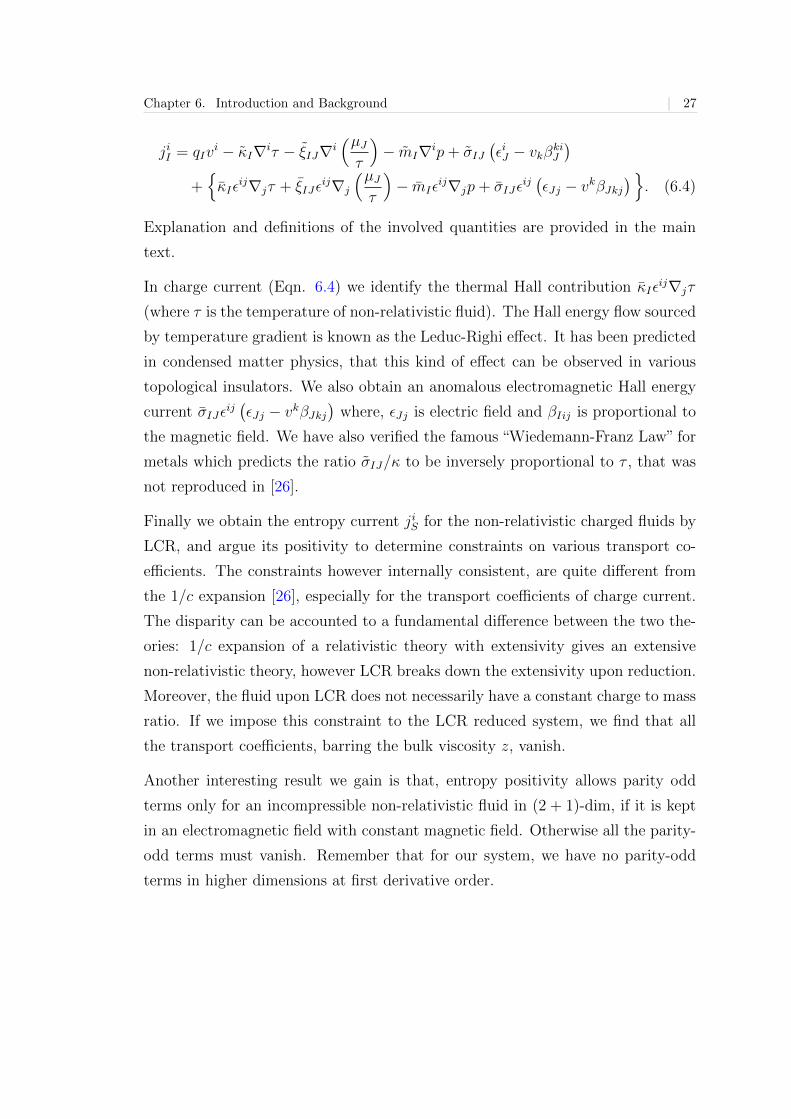
Chapter 6. Introduction and Background | 27
jiI = qIvi − κI∇iτ − ξIJ∇i
(µJτ
)− mI∇ip+ σIJ
(εiJ − vkβkiJ
)+κIε
ij∇jτ + ξIJεij∇j
(µJτ
)− mIε
ij∇jp+ σIJεij(εJj − vkβJkj
). (6.4)
Explanation and definitions of the involved quantities are provided in the main
text.
In charge current (Eqn. 6.4) we identify the thermal Hall contribution κIεij∇jτ
(where τ is the temperature of non-relativistic fluid). The Hall energy flow sourced
by temperature gradient is known as the Leduc-Righi effect. It has been predicted
in condensed matter physics, that this kind of effect can be observed in various
topological insulators. We also obtain an anomalous electromagnetic Hall energy
current σIJεij(εJj − vkβJkj
)where, εJj is electric field and βIij is proportional to
the magnetic field. We have also verified the famous “Wiedemann-Franz Law” for
metals which predicts the ratio σIJ/κ to be inversely proportional to τ , that was
not reproduced in [26].
Finally we obtain the entropy current jiS for the non-relativistic charged fluids by
LCR, and argue its positivity to determine constraints on various transport co-
efficients. The constraints however internally consistent, are quite different from
the 1/c expansion [26], especially for the transport coefficients of charge current.
The disparity can be accounted to a fundamental difference between the two the-
ories: 1/c expansion of a relativistic theory with extensivity gives an extensive
non-relativistic theory, however LCR breaks down the extensivity upon reduction.
Moreover, the fluid upon LCR does not necessarily have a constant charge to mass
ratio. If we impose this constraint to the LCR reduced system, we find that all
the transport coefficients, barring the bulk viscosity z, vanish.
Another interesting result we gain is that, entropy positivity allows parity odd
terms only for an incompressible non-relativistic fluid in (2 + 1)-dim, if it is kept
in an electromagnetic field with constant magnetic field. Otherwise all the parity-
odd terms must vanish. Remember that for our system, we have no parity-odd
terms in higher dimensions at first derivative order.
7 | Review of Hydrodynamics
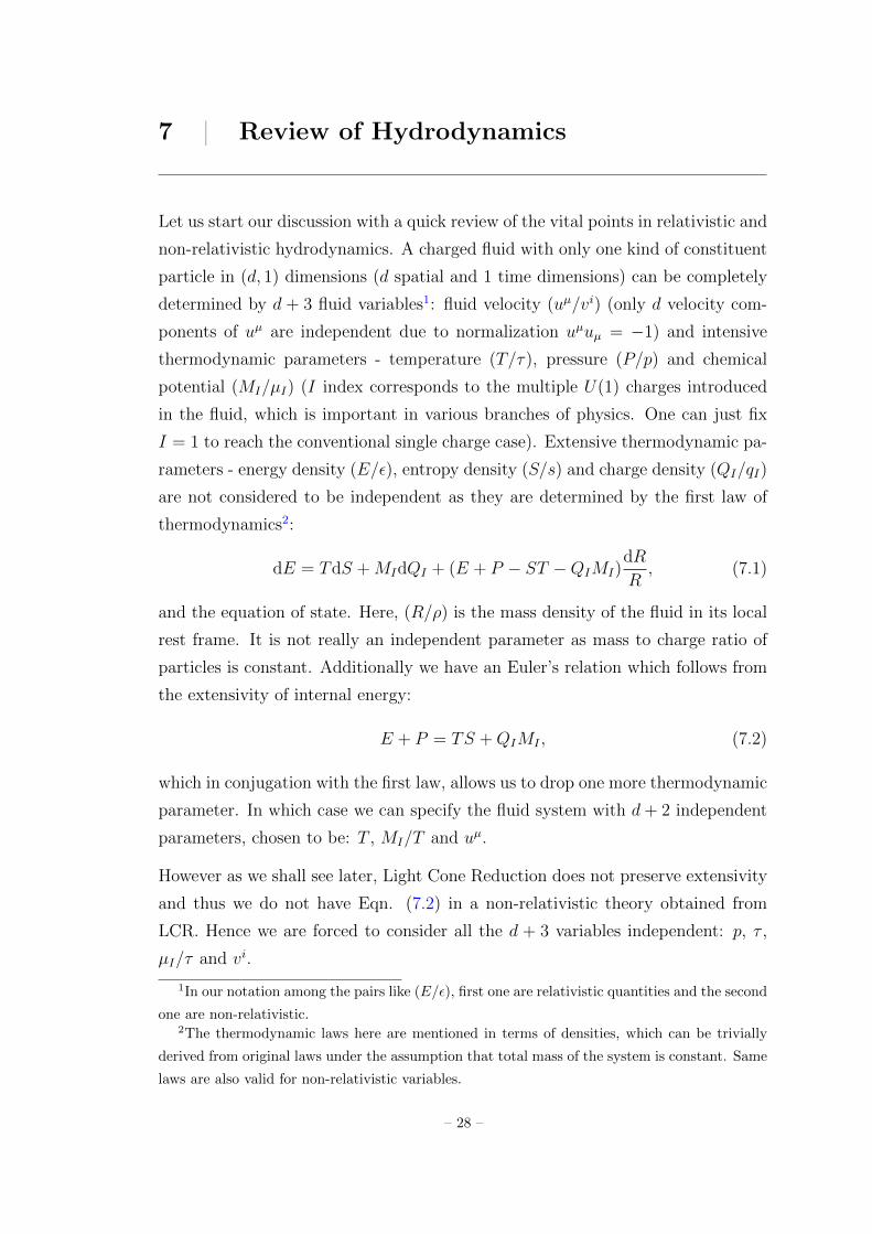
Let us start our discussion with a quick review of the vital points in relativistic and
non-relativistic hydrodynamics. A charged fluid with only one kind of constituent
particle in (d, 1) dimensions (d spatial and 1 time dimensions) can be completely
determined by d + 3 fluid variables1: fluid velocity (uµ/vi) (only d velocity com-
ponents of uµ are independent due to normalization uµuµ = −1) and intensive
thermodynamic parameters - temperature (T/τ), pressure (P/p) and chemical
potential (MI/µI) (I index corresponds to the multiple U(1) charges introduced
in the fluid, which is important in various branches of physics. One can just fix
I = 1 to reach the conventional single charge case). Extensive thermodynamic pa-
rameters - energy density (E/ε), entropy density (S/s) and charge density (QI/qI)
are not considered to be independent as they are determined by the first law of
thermodynamics2:
dE = TdS +MIdQI + (E + P − ST −QIMI)dR
R, (7.1)
and the equation of state. Here, (R/ρ) is the mass density of the fluid in its local
rest frame. It is not really an independent parameter as mass to charge ratio of
particles is constant. Additionally we have an Euler’s relation which follows from
the extensivity of internal energy:
E + P = TS +QIMI , (7.2)
which in conjugation with the first law, allows us to drop one more thermodynamic
parameter. In which case we can specify the fluid system with d+ 2 independent
parameters, chosen to be: T , MI/T and uµ.
However as we shall see later, Light Cone Reduction does not preserve extensivity
and thus we do not have Eqn. (7.2) in a non-relativistic theory obtained from
LCR. Hence we are forced to consider all the d + 3 variables independent: p, τ ,
µI/τ and vi.
1In our notation among the pairs like (E/ε), first one are relativistic quantities and the second
one are non-relativistic.2The thermodynamic laws here are mentioned in terms of densities, which can be trivially
derived from original laws under the assumption that total mass of the system is constant. Same
laws are also valid for non-relativistic variables.
– 28 –

Chapter 7. Review of Hydrodynamics | 29
7.1 Relativistic Hydrodynamics
We consider a relativistic charged fluid in (d + 1, 1) dimensions. The d + 3 in-
dependent fluid parameters (T , MI/T and uµ) are related by d + 3 equations of
motion of the fluid known as constitutive equations. They are nothing but the
conservation equations of energy-momentum and charge:
∇µTµν = 0, ∇µJ
µI = 0, (7.3)
where T µν is the energy-momentum tensor and JµI is the charge current. There-
fore once T µν and JµI are known, fluid is completely determined (along with the
equation of state of-course). For an ideal relativistic fluid (in absence of viscosity
or internal friction) they are given as:
T µν = (E + P )uµuν + Pgµν , Jµ = QIuµ. (7.4)
7.1.1 Viscous Relativistic Fluids in Presence of Background
Fields
An important characteristic of fluids is dissipation. Since fluid is a macroscopic
system, it is governed by the second law of thermodynamics, which says that
total entropy of a system should always increase. Since fluid is assumed to be in
thermodynamic equilibrium at every space-time point, entropy should be created
locally at every point. We will look at it explicitly later, but for now it suffices
to mention that for a system in exact thermodynamic equilibrium (ideal fluid),
the entropy is constant. However, if we slowly depart from the equilibrium by
introducing gradients of control parameters (T,MI/T, uµ) all over the fluid, the
fluid starts to create entropy. This phenomenon is called dissipation.
Since fluid dynamics is nearly in equilibrium, we suppose that the gradients of
T,MI/T, uµ are fairly small, and hence one can rest upon a perturbative expansion
in derivatives. In this work we consider a fluid upto first derivative order.
Further, the fluid can be introduced to some external electromagnetic gauge fields
Aµ, which affect its dynamics. The energy-momentum and charge will no longer
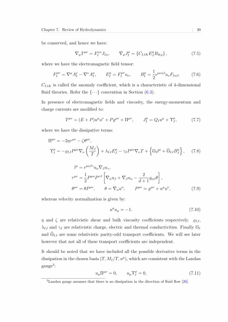
Chapter 7. Review of Hydrodynamics | 30
be conserved, and hence we have:
∇µTµν = F να
I JIα, ∇µJµI = CIJKEµ
JBKµ , (7.5)
where we have the electromagnetic field tensor:
F µνI = ∇µAνI −∇νAµI , Eµ
I = F µνI uν , Bµ
I =1
2εµναβuνFIαβ. (7.6)
CIJK is called the anomaly coefficient, which is a characteristic of 4-dimensional
fluid theories. Refer the · · · convention in Section (6.3).
In presence of electromagnetic fields and viscosity, the energy-momentum and
charge currents are modified to:
T µν = (E + P )uµuν + Pgµν + Πµν , JµI = QIuµ + Υµ
I , (7.7)
where we have the dissipative terms:
Πµν = −2ητµν − ζθµν ,
ΥµI = −%IJP µν∇ν
(MJ
T
)+ λIJE
µJ − γIP
µν∇νT +fI l
µ + fIJBµJ
, (7.8)
lµ = εµαβγuα∇βuγ,
τµν =1
2P µαP νβ
[∇αuβ +∇βuα −
2
d+ 1gαβθ
],
θµν = θP µν , θ = ∇αuα, P µν = gµν + uµuν , (7.9)
whereas velocity normalization is given by:
uµuµ = −1. (7.10)
η and ζ are relativistic shear and bulk viscosity coefficients respectively. %IJ ,
λIJ and γI are relativistic charge, electric and thermal conductivities. Finally fI
and fIJ are some relativistic parity-odd transport coefficients. We will see later
however that not all of these transport coefficients are independent.
It should be noted that we have included all the possible derivative terms in the
dissipation in the chosen basis (T,MI/T, uµ), which are consistent with the Landau
gauge3:
uµΠµν = 0, uµΥµI = 0, (7.11)
3Landau gauge assumes that there is no dissipation in the direction of fluid flow [20].
Chapter 7. Review of Hydrodynamics | 31
Now we have a complete description of relativistic charged fluids in electromagnetic
background upto one derivative order. But, since we are not interested in higher
derivative orders, we can use Eqn. (7.5) at the first derivative level:
uα∇αE = −(E + P )θ, P µα∇αP −QIEµI = −(E + P )uα∇αu
µ,
uµ∇µQI +QIθ = CIJKEµJBKµ . (7.12)
By doing this we are introducing an error at second derivative order, which is to
be neglected. We have also used EµI uµ = 0, which can be checked trivially from
Eqn. (7.6). Using these τµν from Eqn. (7.9) can be written as:
τµν =1
2
[Yµν + Yνµ − 2
d+ 1gµνθ − Zuµuν
], (7.13)
where,
Z =2
d+ 1
uα∇αT
(E + P ), T = (d+ 1)P − E,
Yµν = ∇µuν − uν∇µP
E + P+QI
uνEµI
E + P. (7.14)
T has been defined for a convenient switchover to conformal fluids, which are of
abundant interest in physics; for instance in the first part of this thesis report.
Conformal fluids are those whose energy-momentum tensor is traceless:
T µµ = T− ζ(d+ 1)θ = 0, (7.15)
which can be reached just by setting T = ζ = 0.
7.1.2 Entropy Current
Now we turn our attention to the second law of thermodynamics:
∇µJµS ≥ 0. (7.16)
Considering the possibility of creating entropy at every space-time point, we added
the most generic viscous terms to the constitutive equations of the fluid. But it
turns out that not all those terms always create entropy, instead some end up
reducing it. Or in other words, entropy current positivity cannot be ensured
Chapter 7. Review of Hydrodynamics | 32
in the presence of certain dissipative terms with arbitrary transport coefficients.
Hence we get some constraints on these transport coefficients.
The canonical entropy current is given by:
JµS = Suµ − MI
TΥµI , (7.17)
Using Eqn. (7.12) one can then show that:
∇µJµS = − 1
TΠµν∇µuν +
[EIµT−∇µ
(MI
T
)]ΥµI , (7.18)
which only depends on the dissipative terms. This implies that in absence of
dissipation fluid does not create any entropy. Plugging in values of Πµν and Υµ
from Eqn. (7.8) and demanding ∇µJµS ≥ 0, we will obtain the constraints:
γI = 0, η ≥ 0, ζ ≥ 0, λIJ =1
T%IJ ,
%IJ matrix is positive definite. (7.19)
However there are additional parity-odd terms in the charge current that cannot
be made positive definite, corresponding to coefficients fI and fIJ . One would
then expect that these coefficients must vanish. But a fabulous idea was proposed
in [21], where authors modify the entropy current itself with the most generic
parity odd vectors:
JµS → JµS +Dlµ + DIB
µI
, (7.20)
demanding that the contributions of all parity odd terms collectively must vanish.
This demand relates fI , fIJ , D, DI and CIJK as follows:
∂D
∂P=
2D
E + P,
∂D
∂(MI/T )= fI ,
∂DJ
∂P=
DJ
E + P,
∂DJ
∂(MI/T )= fIJ ,
D2QI
E + P− 2DI = − 1
TfI , DJ
QI
E + P= − 1
TfIJ + CKIJ
MK
T.
(7.21)
Now we have a complete description of generic relativistic fluids, with all the first
order dissipative term allowed by entropy positivity.
Chapter 7. Review of Hydrodynamics | 33
7.2 Non-relativistic Fluid Dynamics
Let us now consider a first derivative order, non-relativistic charged fluid in (d, 1)
dimensions, in presence of electromagnetic fields. It would be helpful to contrast
the theory with its relativistic analogue to gain some understanding of similarities
and distinctions. The d+ 3 independent fluid parameters4 (p, τ , µI/τ and vi) are
related by d + 3 constitutive equations, which are the conservation equations of
mass, energy, momentum and charge, respectively:
∂tρ+ ∂i(ρvi) = 0, ∂t
(ε+
1
2ρv2
)+ ∂ij
i = jiIεIi,
∂tqI + ∂ijiI = 0, ∂t(ρv
j) + ∂itij = qIε
jI − jIiβ
ijI , (7.22)
where we can introduce the scalar potential (φ) and vector potential (ai), in terms
of which electric and magnetic fields are given as:
εiI = −∂iφI − ∂taiI , βijI = ∂iajI − ∂jaiI . (7.23)
−jIiβijI translates to qI(~v×(~∇×~aI))i in four dimensional non-viscous fluid. Stress-
energy tensor, energy current and charge current are respectively given by:
tij = ρvivj+pgij+πij, ji =
(ε+ p+
1
2ρv2
)vi+ς i, jiI = qIv
i+ς iI , (7.24)
where we have the dissipative terms:
πij = −nσij − zδij∂kvk
ς i = −nσijvj − z∂kvkvi − κ∂iτ − ξ∇i(µIτ
)+ σIε
iI ,−αIvjβ
jiI ,
ς iI = −κI∇iτ − ξIJ∇i(µJτ
)− mI∇ip+ σIJε
iJ − αIJvkβkiJ
+κIε
ij∇jτ + ξIJεij∇j
(µJτ
)− mIε
ij∇jp+ σIJεijεJj − αIJεijvkβJkj
.
(7.25)
and σij is defined as:
σij = ∂ivj + ∂jvi − δij 2
d∂kv
k. (7.26)
Here n and z are non-relativistic bulk and shear viscosity coefficients respec-
tively. κ, ξI , σI and αI are thermal, charge, electric and magnetic conductivi-
ties. κI , σIJ , ξIJ , mI , αIJ and κI , σIJ , ξIJ , mI , αIJ are some corresponding arbitrary
4Recall that we are not assuming Euler’s relation to hold in the non-relativistic theory.
Chapter 7. Review of Hydrodynamics | 34
parity-even and parity-odd transport coefficients5. Later we shall see that after
light cone reduction of a relativistic fluid theory most of these coefficients are
related.
Note that we are considering mass and charge continuity equations separately,
because as we shall see later, light cone reduction does not enforce mass to charge
ratio of particles to be constant (which is not very encouraging).
This finishes our discussion on the fluid mechanical machinery we would be re-
quiring for further analysis. Interested readers can find a detailed discussion on
fluid dynamics in [20, 23].
5The sign of these coefficients are completely arbitrary for now, and are chosen keeping in
mind later convenience.
8 | Light Cone Reduction
Now that we have reviewed the necessary aspects of hydrodynamics, we are ready
to continue with the main subject matter of this work. As was discussed in
Section (6.2), LCR is a mechanism which connects a (d + 1, 1)-dim relativistic
fluid to a (d, 1)-dim non-relativistic fluid. Essentially we perform the follow-
ing coordinate transformation to the relativistic theory in Minkowski coordinates
xµµ=0,1,..,d+1:
√2x± = x0 ± xd+1, ds2 = −2dx+dx− +
d∑i=1
(dxi)2, (8.1)
to go to light-cone coordinates x±, xii=1,2,..,d. Then, we reduce the theory along
x− direction, identifying x+ with the non-relativistic time (t). This reduces the
underlying symmetry group of relativistic theory (e.g. Poincare or Conformal) to
the symmetry group of the non-relativistic theory (e.g. Galilean or Schrodinger
respectively).
Light cone reduction of the constitutive equations of a relativistic fluid boil down
to the non-relativistic constitutive equations in one dimension lower. Relativistic
charged fluid in (d + 1) + 1 dimensions, as we have already discussed, has d + 3
independent variables: T,MI/T, uµ. On reduction, the non-relativistic fluid in d
spatial dimensions also has total d+3 independent variables: p, τ, µI/τ, vi. This is
because upon reduction system loses its extensivity, which we will check explicitly
later. Our goal is to find a mapping between these independent variables.
8.1 Reduction of Background Fields
Let us start with reducing the background electromagnetic fields. Maxwell’s equa-
tions for the relativistic system are given by:
∇µFµνI = 0. (8.2)
We take the fields to be sourceless, as we assume that our fluid is very weakly
charged to effect the background field configuration. Under light-cone reduction
– 35 –
Chapter 8. Light Cone Reduction | 36
the above equations take the following form:
~∇2A+I = 0, ∇i
(∇iA−I +∇+A
iI
)= −∇2
+A+I , ∇i
(∇iAjI −∇
jAiI)
= ∇j∇+A+I .
(8.3)
These equations can be identified with source free static Maxwell’s equations of a
non-relativistic system if we map1:
A−I = φI , AiI = aiI , A+I = constant (8.4)
8.2 Reduction of Energy-Momentum and Charge
The reduction of relativistic equations of energy-momentum and charge conserva-
tion after using Eqn. (8.4) gives:
∇+T++ +∇iT
i+ = 0,
∇+T+− +∇iT
i− = −J iI(∇iA
−I +∇+AIi
),
∇+T+j +∇iT
ij = −J+I
(∇+A
jI +∇jA−I
)− J iI
(∇iA
jI −∇
jAIi),
∇+J+I +∇iJ
iI = 0, (8.5)
which reduce to non-relativistic equations under following identifications:
T++ = ρ, T i+ = ρvi, T+− = ε+1
2ρv2, T i− = ji, T ij = tij,
J+I = qI , J iI = jiI . (8.6)
Carrying out this identification at first derivative order will explicitly give the
following form of non-relativistic fluid variables:
ρ = (E + P )(u+)2 + (u+)2 (ηZ− ζθ) , vi =ui
u+− η
ρYi,
p = P −(η
dZ− ζ u
α∇αP
E + P
), ε =
1
2(E − P )− 1
2(ηZ− ζθ) ,
τ =T
u++O(1), µI =
MI
u++O(1),
ji = vi(ε+ p+
1
2ρv2
)−nσikvk− zvi∇kv
k−κ∇iτ − τσI∇i(µIτ
)+σI(ε
iI − vjβ
jiI )
1In Appendix (B.1) we have discussed direct non-relativistic limit of Maxwell’s equations.
Chapter 8. Light Cone Reduction | 37
qI = u+QI − u+[%IJu
ν∇ν
(MJ
T
)+ γIu
ν∇νT +fIε
iju+∇ivj + fIJεijβijJ
]
jiI = qivi − κI∇iτ − ξIJ∇i
(µJτ
)− mI∇ip+ σIJ
(εiJ − vkβkiJ
)+κIε
ij∇jτ + ξIJεij∇j
(µJτ
)− mIε
ij∇jp+ σIJεij(εJj − vkβJkj
). (8.7)
and transport coefficients:
n = ηu+, z = ζu+, κ = 2nε+ p
τρ, ξ = τσI = n
qIτ
ρ
mI =γIτu
+
2(ε+ p), ξIJ =
[%IJ +
ξJqI2(ε+ p)
−mIqJτ
],
κI =κqI
2(ε+ p), σIJ = αIJ =
[λIJu
+ +σJqI
2(ε+ p)
],
mI =2ωIρ, ξIJ = ξJ
ωIn, κI = κ
ωIn, σIJ = αIJ =
[σJωIn− 2ωIJ
],
(8.8)
where,
ωI = fI(u+)2, ωIJ = fIJu
+. (8.9)
Note that after identification not all transport coefficients are independent; only
independent coefficients are: n, z, mI , ξIJ , σIJ , ωI and ωIJ .
Wiedemann-Franz Law: This famous law predicts the ratio of charge conduc-
tivity (which appears in charge current)2 to thermal conductivity (which appears
in energy current) in metals as: σ/κ = 1/Lτ , where L is the Lorenz number pre-
dicted to be ∼ 2.45 × 10⁻⁸ WΩK−2. The law is found to be in good agreement
with experiments. We attempt to check the same in our setup3:
σ
κ=
ρ%
2n(ε+ p)+
τq2
4(ε+ p)2, (8.10)
We model the electrons in metals as free classical gas with no external pressure:
fluid with homogeneous particles each of charge e (electronic charge), mass me
2There is only one U(1) charge here.3We have used here the fact that non-relativistic system respects the constraint τ σIJ = ξIJ ,
which has been showed in next section.
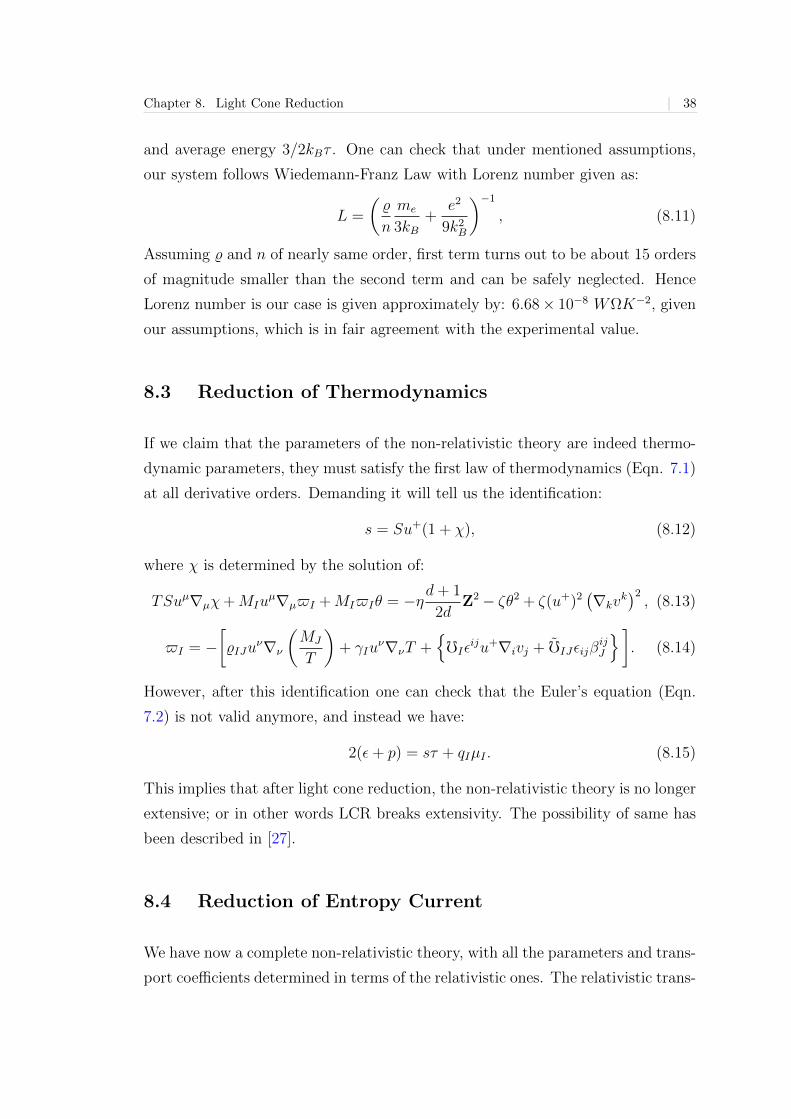
Chapter 8. Light Cone Reduction | 38
and average energy 3/2kBτ . One can check that under mentioned assumptions,
our system follows Wiedemann-Franz Law with Lorenz number given as:
L =
(%
n
me
3kB+
e2
9k2B
)−1, (8.11)
Assuming % and n of nearly same order, first term turns out to be about 15 orders
of magnitude smaller than the second term and can be safely neglected. Hence
Lorenz number is our case is given approximately by: 6.68× 10⁻⁸ WΩK−2, given
our assumptions, which is in fair agreement with the experimental value.
8.3 Reduction of Thermodynamics
If we claim that the parameters of the non-relativistic theory are indeed thermo-
dynamic parameters, they must satisfy the first law of thermodynamics (Eqn. 7.1)
at all derivative orders. Demanding it will tell us the identification:
s = Su+(1 + χ), (8.12)
where χ is determined by the solution of:
TSuµ∇µχ+MIuµ∇µ$I +MI$Iθ = −ηd+ 1
2dZ2− ζθ2 + ζ(u+)2
(∇kv
k)2, (8.13)
$I = −[%IJu
ν∇ν
(MJ
T
)+ γIu
ν∇νT +fIε
iju+∇ivj + fIJεijβijJ
]. (8.14)
However, after this identification one can check that the Euler’s equation (Eqn.
7.2) is not valid anymore, and instead we have:
2(ε+ p) = sτ + qIµI . (8.15)
This implies that after light cone reduction, the non-relativistic theory is no longer
extensive; or in other words LCR breaks extensivity. The possibility of same has
been described in [27].
8.4 Reduction of Entropy Current
We have now a complete non-relativistic theory, with all the parameters and trans-
port coefficients determined in terms of the relativistic ones. The relativistic trans-
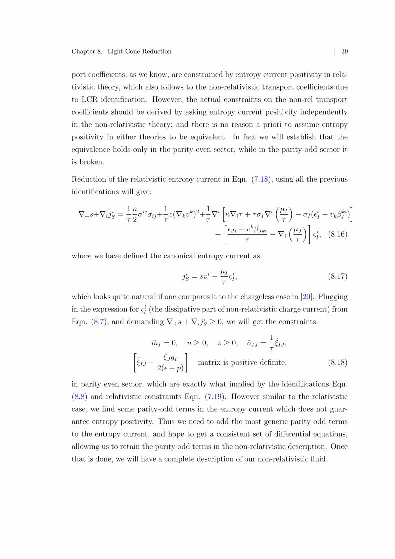
Chapter 8. Light Cone Reduction | 39
port coefficients, as we know, are constrained by entropy current positivity in rela-
tivistic theory, which also follows to the non-relativistic transport coefficients due
to LCR identification. However, the actual constraints on the non-rel transport
coefficients should be derived by asking entropy current positivity independently
in the non-relativistic theory; and there is no reason a priori to assume entropy
positivity in either theories to be equivalent. In fact we will establish that the
equivalence holds only in the parity-even sector, while in the parity-odd sector it
is broken.
Reduction of the relativistic entropy current in Eqn. (7.18), using all the previous
identifications will give:
∇+s+∇ijiS =
1
τ
n
2σijσij+
1
τz(∇kv
k)2+1
τ∇i[κ∇iτ + τσI∇i
(µIτ
)− σI(εiI − vkβkiI )
]+
[εJi − vkβJki
τ−∇i
(µJτ
)]ς iI , (8.16)
where we have defined the canonical entropy current as:
jiS = svi − µIτς iI , (8.17)
which looks quite natural if one compares it to the chargeless case in [20]. Plugging
in the expression for ς iI (the dissipative part of non-relativistic charge current) from
Eqn. (8.7), and demanding ∇+s+∇ijiS ≥ 0, we will get the constraints:
mI = 0, n ≥ 0, z ≥ 0, σIJ =1
τξIJ ,[
ξIJ −ξJqI
2(ε+ p)
]matrix is positive definite, (8.18)
in parity even sector, which are exactly what implied by the identifications Eqn.
(8.8) and relativistic constraints Eqn. (7.19). However similar to the relativistic
case, we find some parity-odd terms in the entropy current which does not guar-
antee entropy positivity. Thus we need to add the most generic parity odd terms
to the entropy current, and hope to get a consistent set of differential equations,
allowing us to retain the parity odd terms in the non-relativistic description. Once
that is done, we will have a complete description of our non-relativistic fluid.
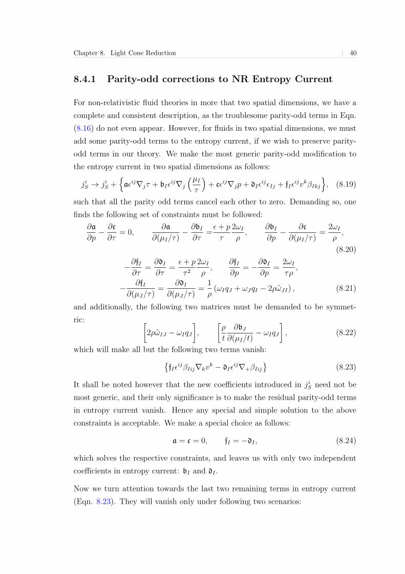
Chapter 8. Light Cone Reduction | 40
8.4.1 Parity-odd corrections to NR Entropy Current
For non-relativistic fluid theories in more that two spatial dimensions, we have a
complete and consistent description, as the troublesome parity-odd terms in Eqn.
(8.16) do not even appear. However, for fluids in two spatial dimensions, we must
add some parity-odd terms to the entropy current, if we wish to preserve parity-
odd terms in our theory. We make the most generic parity-odd modification to
the entropy current in two spatial dimensions as follows:
jiS → jiS +aεij∇jτ + bIε
ij∇j
(µIτ
)+ cεij∇jp+ dIε
ijεIj + fIεijvkβIkj
, (8.19)
such that all the parity odd terms cancel each other to zero. Demanding so, one
finds the following set of constraints must be followed:
∂a
∂p− ∂c
∂τ= 0,
∂a
∂(µI/τ)− ∂bI
∂τ=ε+ p
τ
2ωIρ,
∂bI∂p− ∂c
∂(µI/τ)=
2ωIρ,
(8.20)
−∂fI∂τ
=∂dI∂τ
=ε+ p
τ 22ωIρ,
∂fI∂p
= −∂dI∂p
=2ωIτρ
,
− ∂fI∂(µJ/τ)
=∂dI
∂(µJ/τ)=
1
ρ(ωIqJ + ωJqI − 2ρωJI) , (8.21)
and additionally, the following two matrices must be demanded to be symmet-
ric: [2ρωIJ − ωIqJ
],
[ρ
t
∂bJ∂(µI/t)
− ωIqJ], (8.22)
which will make all but the following two terms vanish:fIε
ijβIij∇kvk − dIε
ij∇+βIij
(8.23)
It shall be noted however that the new coefficients introduced in jiS need not be
most generic, and their only significance is to make the residual parity-odd terms
in entropy current vanish. Hence any special and simple solution to the above
constraints is acceptable. We make a special choice as follows:
a = c = 0, fI = −dI , (8.24)
which solves the respective constraints, and leaves us with only two independent
coefficients in entropy current: bI and dI .
Now we turn attention towards the last two remaining terms in entropy current
(Eqn. 8.23). They will vanish only under following two scenarios:
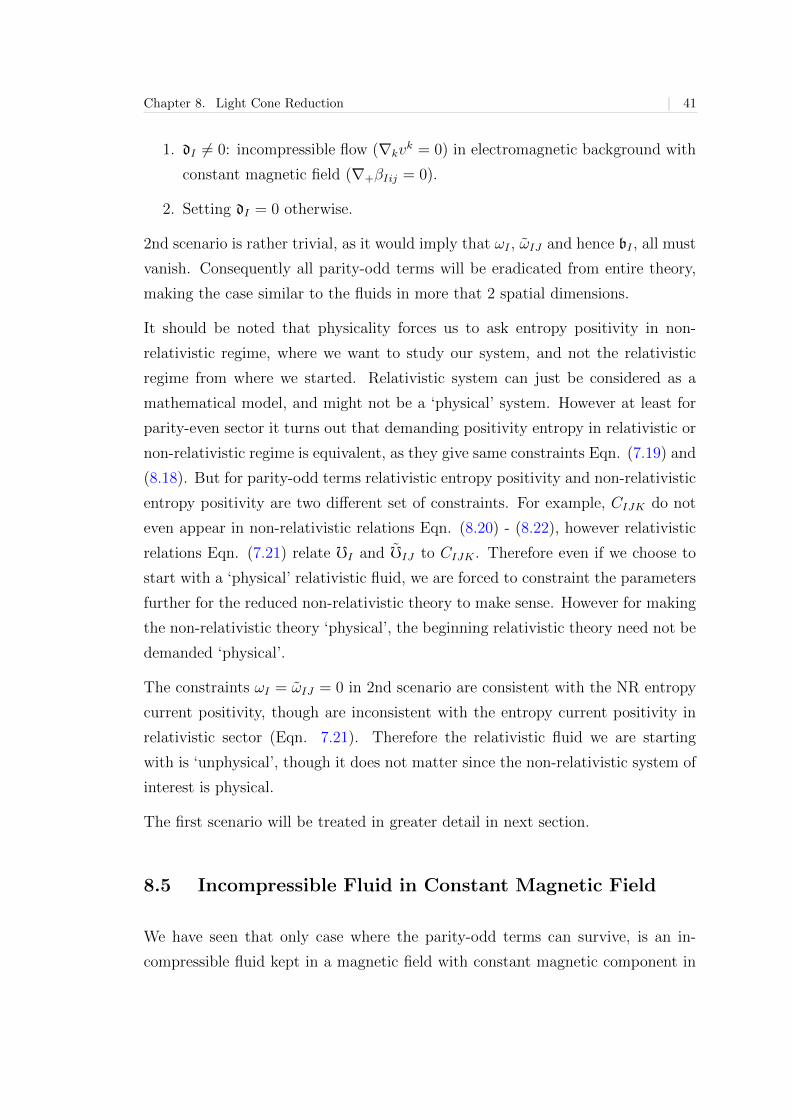
Chapter 8. Light Cone Reduction | 41
1. dI 6= 0: incompressible flow (∇kvk = 0) in electromagnetic background with
constant magnetic field (∇+βIij = 0).
2. Setting dI = 0 otherwise.
2nd scenario is rather trivial, as it would imply that ωI , ωIJ and hence bI , all must
vanish. Consequently all parity-odd terms will be eradicated from entire theory,
making the case similar to the fluids in more that 2 spatial dimensions.
It should be noted that physicality forces us to ask entropy positivity in non-
relativistic regime, where we want to study our system, and not the relativistic
regime from where we started. Relativistic system can just be considered as a
mathematical model, and might not be a ‘physical’ system. However at least for
parity-even sector it turns out that demanding positivity entropy in relativistic or
non-relativistic regime is equivalent, as they give same constraints Eqn. (7.19) and
(8.18). But for parity-odd terms relativistic entropy positivity and non-relativistic
entropy positivity are two different set of constraints. For example, CIJK do not
even appear in non-relativistic relations Eqn. (8.20) - (8.22), however relativistic
relations Eqn. (7.21) relate fI and fIJ to CIJK . Therefore even if we choose to
start with a ‘physical’ relativistic fluid, we are forced to constraint the parameters
further for the reduced non-relativistic theory to make sense. However for making
the non-relativistic theory ‘physical’, the beginning relativistic theory need not be
demanded ‘physical’.
The constraints ωI = ωIJ = 0 in 2nd scenario are consistent with the NR entropy
current positivity, though are inconsistent with the entropy current positivity in
relativistic sector (Eqn. 7.21). Therefore the relativistic fluid we are starting
with is ‘unphysical’, though it does not matter since the non-relativistic system of
interest is physical.
The first scenario will be treated in greater detail in next section.
8.5 Incompressible Fluid in Constant Magnetic Field
We have seen that only case where the parity-odd terms can survive, is an in-
compressible fluid kept in a magnetic field with constant magnetic component in
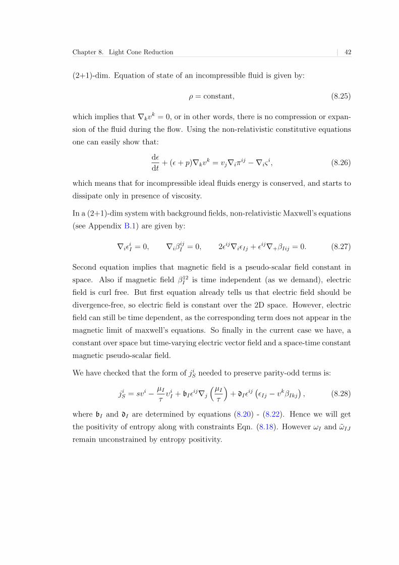
Chapter 8. Light Cone Reduction | 42
(2+1)-dim. Equation of state of an incompressible fluid is given by:
ρ = constant, (8.25)
which implies that ∇kvk = 0, or in other words, there is no compression or expan-
sion of the fluid during the flow. Using the non-relativistic constitutive equations
one can easily show that:
dε
dt+ (ε+ p)∇kv
k = vj∇iπij −∇iς
i, (8.26)
which means that for incompressible ideal fluids energy is conserved, and starts to
dissipate only in presence of viscosity.
In a (2+1)-dim system with background fields, non-relativistic Maxwell’s equations
(see Appendix B.1) are given by:
∇iεiI = 0, ∇iβ
ijI = 0, 2εij∇iεIj + εij∇+βIij = 0. (8.27)
Second equation implies that magnetic field is a pseudo-scalar field constant in
space. Also if magnetic field β12I is time independent (as we demand), electric
field is curl free. But first equation already tells us that electric field should be
divergence-free, so electric field is constant over the 2D space. However, electric
field can still be time dependent, as the corresponding term does not appear in the
magnetic limit of maxwell’s equations. So finally in the current case we have, a
constant over space but time-varying electric vector field and a space-time constant
magnetic pseudo-scalar field.
We have checked that the form of jiS needed to preserve parity-odd terms is:
jiS = svi − µIτυiI + bIε
ij∇j
(µIτ
)+ dIε
ij(εIj − vkβIkj
), (8.28)
where bI and dI are determined by equations (8.20) - (8.22). Hence we will get
the positivity of entropy along with constraints Eqn. (8.18). However ωI and ωIJ
remain unconstrained by entropy positivity.
9 | Discussion
We started with a generic (d + 2)-dim non-conformal relativistic fluid (d ≥ 2)
with anomalies specific to d = 2 in presence of background fields on flat space.
Light cone reduction of this system gave a (d + 1)-dim non-relativistic fluid with
anomalies (specific to d = 2). On physical basis of entropy positivity, we deduced
that parity odd terms in non-relativistic theory can only sustain for incompressible
fluid in electromagnetic background with constant magnetic field in (2 + 1)-dim.
Otherwise for a generic fluid in (d + 1)-dim (d > 2), or for compressible fluid, or
a fluid in time-variable magnetic field in (2 + 1)-dim, the parity odd terms must
disappear.
The theory we gain by LCR is purely ‘Galilean’, as the reduction is done at the
level of algebra. Therefore we have generic1 dissipative terms in our non-relativistic
fluid, which are allowed by the symmetry and the entropy positivity. LCR does
not constraint the size of these coefficients however, and they as well might be
infinitesimal and hence not present in practical conditions. On the contrary, when
one performs a 1/c expansion [22], many of these terms are suppressed depending
on the physical considerations and the type of system under view. We discuss the
basic aspects of 1/c expansion in Appendix (B.2).
Apart from the dissipation terms, ours and the non-relativistic system of [22]
have certain fundamental differences. Firstly, their system is ‘extensive’ as the
thermodynamic variables follow Euler’s relation; however since LCR breaks the
Euler’s relation, our system is no longer extensive. Secondly, in our system ρ is
not necessarily proportional to qI , while in [22] it is true at least at the leading
1/c order. This is why our non-relativistic system has one more independent
parameter as opposed to the 1/c case. We can however enforce ρ ∝ qI in our
system as well, but it turns out that demanding so switches off all the dissipative
terms from the theory except for the bulk viscosity.
In [22] authors do not present a entropy current calculation for non-relativistic
fluid obtained by 1/c expansion. In fact, as we will review in Appendix (B.2), the
1Word generic here just mean possible, and not all possible. We might have more or less
terms, depending on the type of relativistic theory we are starting with and the identification.
– 43 –
Chapter 9. Discussion | 44
entropy positivity in turns out to be trivial, and is just followed from the leading
order entropy current of the relativistic theory. The constraints on the transport
coefficients (which survives at the leading order) also turns out to be the same.
However in our case, we have slightly different constraints, because of the above
mentioned fundamental differences between the two cases.
PART - III
Appendix
A Holographic Ferromagnetism 46
A.1 Background Subtraction . . . . . . . . . . . . . . . . . . . . . . . . 46
A.2 Critical Points and M vs. B Plots . . . . . . . . . . . . . . . . . . 47
A.3 Magnetization from the Minima of Free Energy . . . . . . . . . . . 48
A.4 Details of Diamagnetic and Paramagnetic Phases . . . . . . . . . . 51
B Non-relativistic Charged Hydrodynamics 53
B.1 Non-relativistic Electromagnetism . . . . . . . . . . . . . . . . . . . 53
B.2 1/c Expansion of Relativistic Fluid Dynamics . . . . . . . . . . . . 55
B.2.1 1/c Expansion of Thermodynamics . . . . . . . . . . . . . . 57
– 45 –
A | Holographic Ferromagnetism
A.1 Background Subtraction
We calculate on-shell action by subtracting the contribution of an extremal mag-
netically charged black hole with magnetic charge qM . The reason to choose this
particular background depends on our choice of ensemble (see [11]). The extremal
black solution is given by equation (2.3) and (2.4) with qE → 0
fe(r) =
(1 +
r2
b2− 2Me
r+q2Mr2
). (A.1)
We consider that the extremal black hole has a constant electric potential which
is same as ΦE of the black hole. The black hole has a horizon radius re, given
by
fe(re) =
(1 +
r2eb2− 2Me
re+q2Mr2e
)= 0. (A.2)
The extremality condition is given by
r2e +3r4eb2
= q2M . (A.3)
Therefore, the on-shell action of background turns out to be
IE =1
16π
∫ R
re
d4x√g
(F 2 +
6
b2
)=β′
4
[−2q2MR
+6R3
3b2− −2qM2
re− 6r3e
3b2
](A.4)
where, β′ is the radius of the Euclidean time circle of background. β′ can be ob-
tained by identifying the asymptotic boundary geometry of the black hole space-
time and extremal black hole spacetime
β√gττ = β′
√geττ .
Thus, we get
β′ = β
(1− (M −Me)b
2
R3
). (A.5)
Subtracting the contribution of extremal black hole on-shell action from that of
black hole we finally get,
Ionshell = IBH − IE =β
4
[−Φ2
Er+ +3q2Mr+−r3+b2
+ r+ − 4re −8r3eb2
]. (A.6)
– 46 –
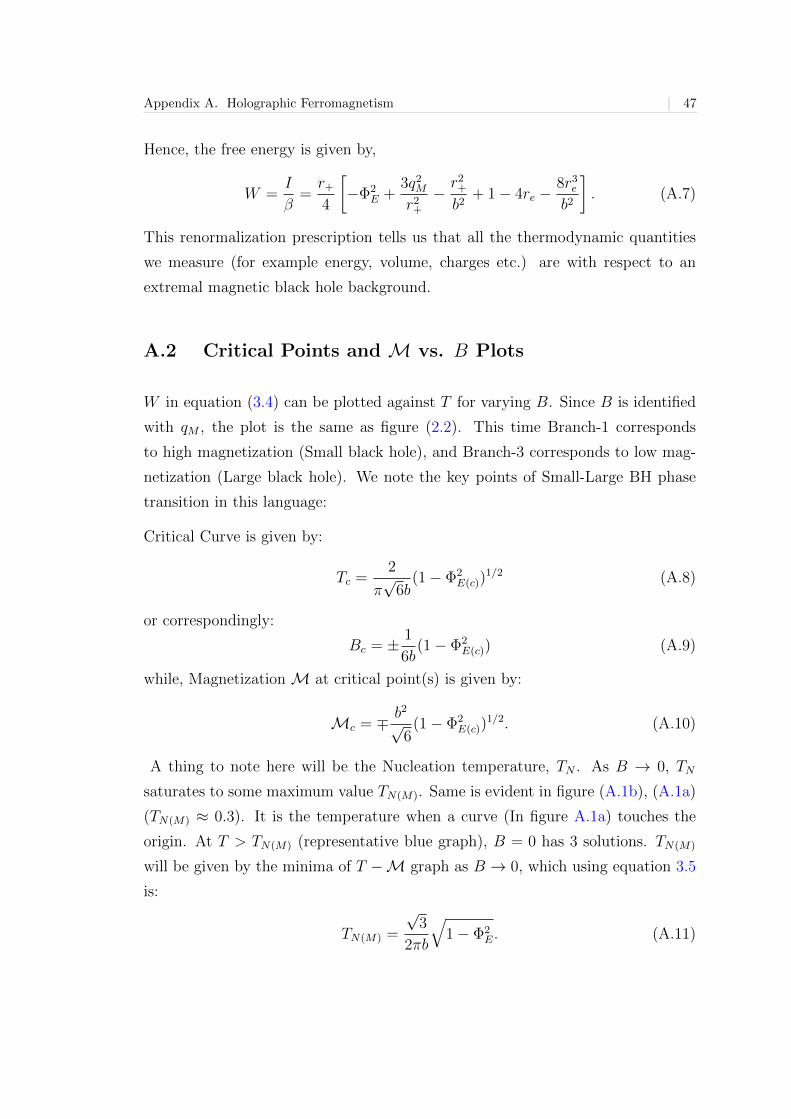
Appendix A. Holographic Ferromagnetism | 47
Hence, the free energy is given by,
W =I
β=r+4
[−Φ2
E +3q2Mr2+−r2+b2
+ 1− 4re −8r3eb2
]. (A.7)
This renormalization prescription tells us that all the thermodynamic quantities
we measure (for example energy, volume, charges etc.) are with respect to an
extremal magnetic black hole background.
A.2 Critical Points and M vs. B Plots
W in equation (3.4) can be plotted against T for varying B. Since B is identified
with qM , the plot is the same as figure (2.2). This time Branch-1 corresponds
to high magnetization (Small black hole), and Branch-3 corresponds to low mag-
netization (Large black hole). We note the key points of Small-Large BH phase
transition in this language:
Critical Curve is given by:
Tc =2
π√
6b(1− Φ2
E(c))1/2 (A.8)
or correspondingly:
Bc = ± 1
6b(1− Φ2
E(c)) (A.9)
while, Magnetization M at critical point(s) is given by:
Mc = ∓ b2√6
(1− Φ2E(c))
1/2. (A.10)
A thing to note here will be the Nucleation temperature, TN . As B → 0, TN
saturates to some maximum value TN(M). Same is evident in figure (A.1b), (A.1a)
(TN(M) ≈ 0.3). It is the temperature when a curve (In figure A.1a) touches the
origin. At T > TN(M) (representative blue graph), B = 0 has 3 solutions. TN(M)
will be given by the minima of T −M graph as B → 0, which using equation 3.5
is:
TN(M) =
√3
2πb
√1− Φ2
E. (A.11)
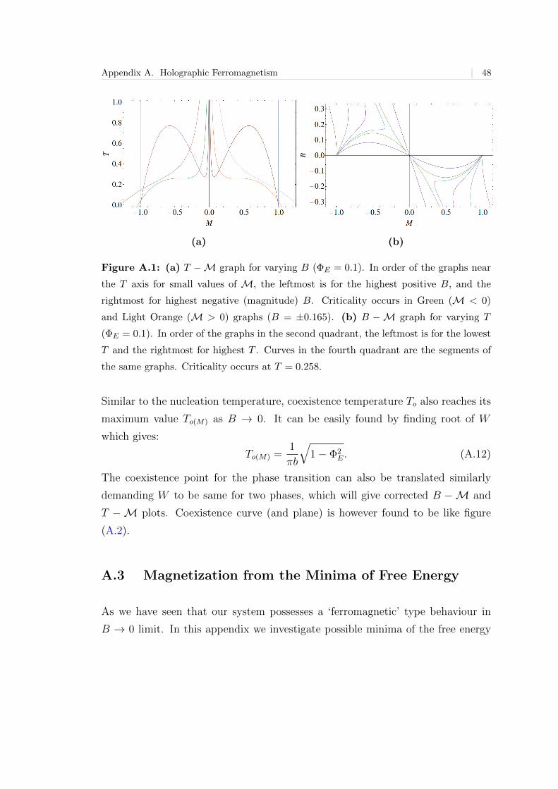
Appendix A. Holographic Ferromagnetism | 48
(a) (b)
Figure A.1: (a) T −M graph for varying B (ΦE = 0.1). In order of the graphs near
the T axis for small values of M, the leftmost is for the highest positive B, and the
rightmost for highest negative (magnitude) B. Criticality occurs in Green (M < 0)
and Light Orange (M > 0) graphs (B = ±0.165). (b) B −M graph for varying T
(ΦE = 0.1). In order of the graphs in the second quadrant, the leftmost is for the lowest
T and the rightmost for highest T . Curves in the fourth quadrant are the segments of
the same graphs. Criticality occurs at T = 0.258.
Similar to the nucleation temperature, coexistence temperature To also reaches its
maximum value To(M) as B → 0. It can be easily found by finding root of W
which gives:
To(M) =1
πb
√1− Φ2
E. (A.12)
The coexistence point for the phase transition can also be translated similarly
demanding W to be same for two phases, which will give corrected B −M and
T −M plots. Coexistence curve (and plane) is however found to be like figure
(A.2).
A.3 Magnetization from the Minima of Free Energy
As we have seen that our system possesses a ‘ferromagnetic’ type behaviour in
B → 0 limit. In this appendix we investigate possible minima of the free energy
Appendix A. Holographic Ferromagnetism | 49
Figure A.2: Black Curve is the Critical Curve in T −B − ΦE plane. The manifold is
the coexistence plane. Above this plane lies the Small BH, and below it Large BH.
as function of temperature. We write the free energy from equation (3.4):
W = M − TS − ΦEqE, (A.13)
= −1
2
(B
M
)(1− Φ2
E)b4 − BM2− b10
2
(B
M
)3
− πTb8(B
M
)2
. (A.14)
Using positive definiteness of r+ we can write
W =1
2
∣∣∣∣ BM∣∣∣∣ (1− Φ2
E)b4 +|BM|
2+b10
2
∣∣∣∣ BM∣∣∣∣3 − πTb8 ∣∣∣∣ BM
∣∣∣∣2 . (A.15)
∂W/∂M = 0 will give us the back the equation of state (equation 3.5), and we
will recover figure (A.1a) and (A.1b). To find the stable solutions ofM in B → 0
limit, we study the extremas of W using (A.14). For r+ = −b4 BM
∣∣∣∣B→0
= 0 we
will have:
M = ±b2√
(1− Φ2E). (A.16)
Whereas for r+ 6= 0 the only solution is:
M = 0 if T ≥ TN(M) =
√3
2πb
√(1− Φ2
E). (A.17)
First one is the background AdS solution which has some net finite magnetization
even without any magnetic field. The second solution however corresponds to large
black hole. The bound on the temperature is nothing but the maximum nucleation
temperature (equation A.11), above which (for B = 0) there will always exist large
Appendix A. Holographic Ferromagnetism | 50
black hole solution with radius
r+(LBH) =2πb2
3
(T +
√T 2 − T 2
N(M)
). (A.18)
To argue the dominance of the above solutions, we express W in the convenient
form of r+ in B → 0.
W =r+2b4[(1− Φ2
E)b4 +M2 + b2r2+ − 2πTb4r+]. (A.19)
For AdS solution, M = ±√
1− Φ2E and r+ = 0, so the free energy vanishes. For
the large black hole solution the free energy is given by
W0 =1
2r+(LBH)
[(1− Φ2
E) +r2+(LBH)
b2− 2πTr+(LBH)
]. (A.20)
When large black hole solution dominates over the global AdS then W < 0. Using
equation (A.18) which boils down to:
T > To(M) =1
πb
√1− Φ2
E. (A.21)
This bound is the maximum coexistence temperature (equation A.12), the temper-
ature at which AdS and large black hole coexist at B = 0. Above To(M), M = 0
solution dominates, while below it M = ±√
1− Φ2E dominates. But the latter
two have the same free energy (equation A.20). Thus system has to spontaneously
choose between these two solutions. As soon as B is applied one of the solutions
disappears1, and system has a preferred direction. This behavior has similarity
with ferromagnetic system.
Notice that the free energy is always zero in B → 0 limit (except for M = 0).
However we can have some insight if we plot W/|B| instead, which keeps the
extremas of W unaltered2 (figure A.3).
Ideally one would be tempted to Taylor expand equation (A.15) nearM = 0, and
construct a Landau-type model to see the symmetry breaking explicitly. However
this is not feasible in our case, as W/|B| is discontinuous and diverging atM = 0
due to the inclusion of |M|, and thus the Taylor expansion breaks down.
1Since B and M must have opposite signs, one of the solutions of M vanishes depending on
the sign of B.2We cannot divide by B as its sign has a dependence on M due to positivity of r+
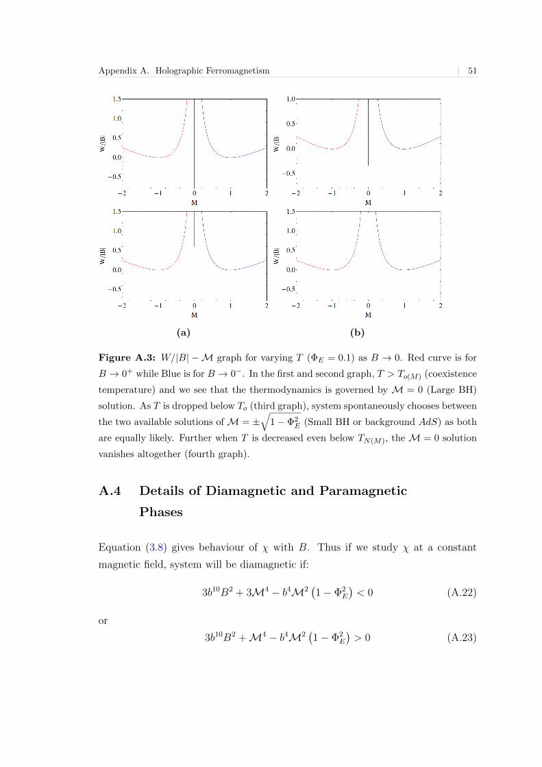
Appendix A. Holographic Ferromagnetism | 51
(a) (b)
Figure A.3: W/|B| −M graph for varying T (ΦE = 0.1) as B → 0. Red curve is for
B → 0+ while Blue is for B → 0−. In the first and second graph, T > To(M) (coexistence
temperature) and we see that the thermodynamics is governed by M = 0 (Large BH)
solution. As T is dropped below To (third graph), system spontaneously chooses between
the two available solutions ofM = ±√
1− Φ2E (Small BH or background AdS) as both
are equally likely. Further when T is decreased even below TN(M), the M = 0 solution
vanishes altogether (fourth graph).
A.4 Details of Diamagnetic and Paramagnetic
Phases
Equation (3.8) gives behaviour of χ with B. Thus if we study χ at a constant
magnetic field, system will be diamagnetic if:
3b10B2 + 3M4 − b4M2(1− Φ2
E
)< 0 (A.22)
or
3b10B2 +M4 − b4M2(1− Φ2
E
)> 0 (A.23)
Appendix A. Holographic Ferromagnetism | 52
and otherwise paramagnetic. That is diamagnetic solution is given by:
M <b4
2
((1− Φ2
E
)−√
(1− Φ2E)
2 − 12b2B2
)(A.24)
b4
6
((1− Φ2
E
)−√
(1− Φ2E)
2 − 36b2B2
)<M
<b4
6
((1− Φ2
E
)+
√(1− Φ2
E)2 − 36b2B2
)(A.25)
M >b4
2
((1− Φ2
E
)+
√(1− Φ2
E)2 − 12b2B2
). (A.26)
The middle one is however the unstable phase. If,
|B| > B∗ =1
2√
3b
(1− Φ2
E
)(A.27)
the system will always be diamagnetic regardless of temperature (figure 1.3a).
However if,
B∗ > |B| > |Bc| (A.28)
the system will have three phases: diamagnetic, paramagnetic and another dia-
magnetic (figure 1.3b).
If the magnetic field is even below Bc, system shows the full feature of 5 phases.
But as we go below the critical point, we know that there comes an unstable
branch which is omitted by the Maxwell’s equal area law (figure 3.1). While we
do so, a section of the small and large BH is also omitted. As a result below a
particular magnetic field B#, the paramagnetic phase of large BH gets cutout and
the only stable solution of large BH is diamagnetic phase. B# will be given by the
point where the coexistence magnetic field is same as the χ = 0 point for a B−Misotherm. For ΦE = 0 and b = 1 we find B# ≈ 0.154 whereas Bc = 0.167.
B | Non-relativistic Charged
Hydrodynamics
B.1 Non-relativistic Electromagnetism
Maxwell’s Electrodynamics is a relativistic theory. In fact it was a precursor to
Einstein’s Special Theory of Relativity. Having a consistent relativistic description
of electrodynamics, eradicated any need for a ‘non-relativistic’ theory of electro-
dynamics. However as in current context, one needs a Galilean description of elec-
trodynamics, just to keep it consistent with other non-relativistic theories.
Recently in [22], authors discuss the non-relativistic limit of electrodynamics in
two distinct ways. Depending on the strength of fields1, we can have two dis-
crete non-relativistic limits: | ~E| c| ~B| electric limit and | ~E| c| ~B| magnetic
limit. We find that the light-cone reduction of relativistic sourceless Maxwell’s
equations, under certain identifications, gives magnetic limit of Maxwell’s equa-
tions, which will be our interest of discussion here. A more thorough discussion of
non-relativistic electrodynamics can be found in [22].
In arbitrary dimensions, inhomogeneous Maxwell’s equations are given by:
∇iFi0 = −µocρ, ∇0F
0i +∇jFji = −µoJ i, (B.1)
while the homogeneous ones (Bianchi identities) are:
εαβ···µνσ∇µFνσ = 0, (B.2)
where εαβ···µνσ is the full-rank Levi-Cevita tensor. The last identity follows directly
from the gauge invariant form of F µν = ∇µAν −∇νAµ or the constituent fields2:
Ei = −∇iφ−∇0Ai and F ij = ∇iAj−∇jAi. As LCR gives a non-relativistic theory
with gauge invariance, we are interested in a non-relativistic limit which preserves
1In this section we use the conventional notation for electrodynamics: E for electric field, B
for magnetic field, ρ for charge density, J for charge current etc.2Instead of the conventional magnetic field, we use its 2nd rank dual in our work, as in
arbitrary dimensions we do not have electromagnetic duality and magnetic field does not have
any fixed rank, while its dual has.
– 53 –
Appendix B. Non-relativistic Charged Hydrodynamics | 54
Eqn. (B.2). We will see that the magnetic limit essentially does the same. However
there exists a consistent electric limit as well, where Bianchi identities are broken,
but inhomogeneous Maxwell’s equations are preserved.
In terms of dimensionless fields and sources one can write the inhomogeneous
Maxwell’s equations as:
α∇iEi = ρ, β
∂
∂tEi +∇jF
ji = −βαJ i, (B.3)
and the Bianchi identities as:
εlm···ij∇iEj = −β 1
2εlm···ij
∂
∂tF ij, εm···kij∇kFij = 0 (B.4)
where α and β are some dimensionless constants given by:
α =[E]εo[ρ][L]
, β =[L]
[T ]c. (B.5)
From here we can easily read out, that in non-relativistic limit β 0. To preserve
the Bianchi identities therefore, Ei should be one order smaller than F ij; which
is why this limit is called ‘magnetic limit’. If we measure smallness in terms of a
parameter ε ∼ 1/c, we will have Ei ∼ εn+1 and F ij ∼ εn. Therefore from Eqn.
(B.3), first nontrivial order of ρ ∼ αεn+1, and J i ∼ αεn−1, and inhomogeneous
Maxwell’s Equations (in conventional units) reduce to:
∇iEi =
ρ
εo, ∇jF
ji = −µoJ i. (B.6)
Essentially we have just dropped the displacement current term from the Ampere’s
Law. To explicitly see if this limit is Galilean invariant, one can lookup [22]. These
are the very equations that have been used in Section (8.1) and (8.5).
One can now push the expansion of Eqn. (B.3) to εn+2 order and derive the
continuity equation:∂
∂tρ+∇iJ
i = 0. (B.7)
It should be remembered however that there are mixed orders in this equation and
to the highest order it just states: ∇iJi = 0, which also follows from Eqn. (B.6).
Continuity equation takes its usual form only when first two leading orders of J i
vanish and ρ ∼ J i, but in which case one of the Maxwell’s equations modifies to:
∇jFji = 0. This in conjugation with the Bianchi identity would mean that the
magnetic field is constant over space.
Appendix B. Non-relativistic Charged Hydrodynamics | 55
Finally in conventional units this limit can be summarized as: F ij ∼ Ei ∼ c−n,
and to the maximum order ρ ∼ c−nεo, Ji ∼ c−n+2εo.
B.2 1/c Expansion of Relativistic Fluid Dynamics
In this section we discuss briefly the 1/c expansion limit of relativistic fluid dynam-
ics to get a non-relativistic theory, using the prescription of [26]. We consider here
just a parity-even fluid for comparison with our work. Parity-odd sector in our case
and in [26] are in different hydrodynamic frames and thus are incomparable.
The constitutive equations of a relativistic fluid (with appropriate factors of c)
are:
∇µTµν = cF να
I JIα, ∇µJaµI = 0, (B.8)
where
T µν = (E + P )uµuν + Pgµν + Πµν , JaµI = QIuµ + Υµ
I . (B.9)
Respective dissipative terms are given as:
Πµν = −2ητµν − ζθP µν , ΥµI = − 1
c2TλIJP
µν∇ν
(MJ
T
)+
1
cλIJE
µJ . (B.10)
We can expand E and MI in terms of their potential and kinetic parts:
E = Rc2 + E , MI =1
KmIc
2 +MI . (B.11)
Here mI is the mass is to ‘I’th charge ratio of constituent particles in their local
rest frame, which is assumed to be constant. K is the total number of U(1)
charges. Non-relativistic mass and energy density are related to their relativistic
counterparts as:
ρ = RΓ, ε = EΓ (B.12)
where Γ = (1−v2/c2)−1. Since the fluid under consideration is single component,
R/QI = mI is a constant. Non-relativistic charge density is defined as:
qI = J0I . (B.13)
Pressure and Temperature are however kept same, which to be consistent with the
main text notation we will denote as: τ = T and p = P .
Appendix B. Non-relativistic Charged Hydrodynamics | 56
Before continuing with expansion we need to fix the order of various quantities.
ρ, ε, p, τ, vi can be thought of finite order without much ambiguity. mI on the other
hand is quite sensitive to the kind of system under consideration. Let us consider
a charged fluid made of ‘ions’ where mI ∼ c2; mI cannot be too low, or else the
fluid would start coupling to the background fields. Correspondingly the charge
density qI would be of order c−2. Further, to keep the thermodynamics intact, one
has to assume mI to be of order of c2. Finally, for external fields to have finite
effect (e.g. force) on the fluid, εiI ∼ βijI ∼ c2.
Using this information we can reduce the energy-momentum tensor to:
T 00 = ρc2 +1
2ρv2 + ε+O(1/c)
T i0 = ρvic+
(1
2ρv2 + ε+ p
)vi
c+
1
cπijvj +O(1/c2)
T ij = tij +O(1/c), tij = ρvivj + pgij + πij (B.14)
where we have used:
n =η
c, z =
ζ
c, (B.15)
πij = −n(∇ivj +∇jvi − gij 2
d∇kv
k
)− zgij∇kv
k (B.16)
Energy-momentum conservation equations, at highest order, will then reduce
to:
∂tρ+ ∂i(ρvi) = 0, ∂t(ρv
i) + ∂itij = εiIqI + βijI jIj. (B.17)
It will be worth to mention here the underlying assumption: n, z ∼ 1 which is just
a observational fact. This is precisely the reason why no dissipative corrections
appear to the continuity equation. We can now expand the charge current:
J0I = qI , qI = QIΓ +O(1/c6)
J iI =1
cjiI +O(1/c7), jiI = qIv
i + ς iI (B.18)
where we have used:
σIJ =λIJc, γIJ =
γIJc
(B.19)
ς iI = c2σIJmJ
Kτ∇iτ (B.20)
Appendix B. Non-relativistic Charged Hydrodynamics | 57
Here again we have used a physical input to fix the order of σIJ . We would demand
that in the non-relativistic theory, charge to mass ratio should be a constant.
Therefore charge continuity and mass continuity equations should be the same
upto leading order in 1/c, and hence ς iI should at maximum be of the order of
c−4. It further implies that σIJ ∼ c−8. As a consequence, effects like electric
conductivity are suppressed in whole theory.
Finally we use: ∇µ
(T µ0 − 1
KmIc2JµI)
= 0 to get the energy conservation:
∂t
[1
2ρv2 + ε
]+ ∂i
[vi(
1
2ρv2 + ε+ P
)+ ς i
]= 0, (B.21)
ς i = πijvj − κ∇iτ, (B.22)
where we have identified the thermal conductivity:
κ = σIJc4
K2
maIm
aJ
τ. (B.23)
which is of finite order.
The non-relativistic theory has essentially turned out to be identical to the charge-
less fluid discussed in [20], because for uni-component fluids, charge density serves
just as number density upto a factor. For multi-particle fluids however this might
become more interesting, as then one does not have to expect charge is to mass
ratio to be constant. In fact one can have some chargeless particles also in the
system.
B.2.1 1/c Expansion of Thermodynamics
First law of thermodynamics and the Euler’s relation in the relativistic theory are
given by:
dE = TdS +MIdQI , E + P = TS +MIQI . (B.24)
Under 1/c expansion they reduce to:
dε = εds+ µIdqI , ε+ p = τs+ µIqI , (B.25)
which are just the non-relativistic analogues of the same equations. We therefore
conclude that the non-relativistic system gained by 1/c expansion follows exten-
sivity.
Appendix B. Non-relativistic Charged Hydrodynamics | 58
Now lets have a look at the second law of thermodynamics in the relativistic side,
which mentions: ∇µJµS ≥ 0. From Eqn. (7.18) we know the positive definite form
of entropy current:
∇µJµS =
1
Tητµντµν+
1
Tζθ2+
[EαI
c2T− 1
cPαµ∇µ
(MI
T
)]%IJ
[EJαc2T− 1
cPαν∇ν
(MJ
T
)].
(B.26)
In highest order this equation for non-relativistic systems says that:
∇ts+∇ijiS =
1
2τnσijσij +
1
τz(∇kv
k)
+κ
τ 2(∇iτ
)2. (B.27)
But if we look at the respective coefficients from the relativistic side:
n =η
c≥ 0, z =
ζ
c≥ 0, κ = %IJ
c3
K2
maIm
aJ
T 2≥ 0. (B.28)
We hence see that the relativistic entropy positivity implies non-relativistic entropy
positivity.
Bibliography
[1] S. Dutta, A. Jain and R. Soni, JHEP 1312, 060 (2013) [arXiv:1310.1748 [hep-
th]].
[2] N. Banerjee, S. Dutta, A. Jain and D. Roychowdhury, arXiv:1405.5687 [hep-
th].
[3] J. M. Maldacena, Adv. Theor. Math. Phys. 2, 231 (1998) [hep-th/9711200].
[4] E. Witten, Adv. Theor. Math. Phys. 2, 253 (1998) [hep-th/9802150].
[5] G. Policastro, D. T. Son and A. O. Starinets, Phys. Rev. Lett. 87, 081601
(2001) [hep-th/0104066].
[6] G. Policastro, D. T. Son and A. O. Starinets, JHEP 0209, 043 (2002) [hep-
th/0205052].
[7] S. A. Hartnoll, C. P. Herzog and G. T. Horowitz, Phys. Rev. Lett. 101, 031601
(2008) [arXiv:0803.3295 [hep-th]].
S. A. Hartnoll, C. P. Herzog and G. T. Horowitz, JHEP 0812, 015 (2008)
[arXiv:0810.1563 [hep-th]].
[8] S. A. Hartnoll and P. Kovtun, Phys. Rev. D 76, 066001 (2007) [arXiv:0704.1160
[hep-th]].
[9] M. M. Caldarelli, O. J. C. Dias and D. Klemm, JHEP 0903, 025 (2009)
[arXiv:0812.0801 [hep-th]].
[10] S. A. Hartnoll, P. K. Kovtun, M. Muller and S. Sachdev, Phys. Rev. B 76,
144502 (2007) [arXiv:0706.3215 [cond-mat.str-el]].
[11] A. Chamblin, R. Emparan, C. V. Johnson and R. C. Myers, Phys. Rev. D
60, 064018 (1999) [hep-th/9902170].
[12] V. Balasubramanian and P. Kraus, Commun. Math. Phys. 208, 413 (1999)
[hep-th/9902121].
[13] S. W. Hawking and D. N. Page, Commun. Math. Phys. 87, 577 (1983).
[14] E. Witten, Adv. Theor. Math. Phys. 2, 505 (1998) [hep-th/9803131].
– 59 –
Bibliography | 60
[15] M. Cvetic and S. S. Gubser, JHEP 9904, 024 (1999) [hep-th/9902195].
[16] P. Basu and S. R. Wadia, Phys. Rev. D 73, 045022 (2006) [hep-th/0506203].
[17] D. Yamada and L. G. Yaffe, JHEP 0609, 027 (2006) [hep-th/0602074].
[18] S. Weinberg, “Gravitation and Cosmology - Principles and Applications of
the General Theory of Relativity,”.
[19] P. K. Townsend, gr-qc/9707012.
[20] L.D.Landau & E.M.Lifshitz (1997). Fluid mechanics, Pergamon Press.
[21] D. T. Son and P. Surowka, Phys. Rev. Lett. 103, 191601 (2009)
[arXiv:0906.5044 [hep-th]].
[22] G. Manfredi, Eur. J. Phys. 34 (2013) 859-871 [arXiv:1303.5608 [physics.class-
ph]].
[23] M. Rangamani, Class. Quant. Grav. 26, 224003 (2009) [arXiv:0905.4352 [hep-
th]].
[24] M. Rangamani, Acta Phys. Polon. B 40, 3745 (2009).
[25] M. Rangamani, S. F. Ross, D. T. Son and E. G. Thompson, JHEP 0901, 075
(2009) [arXiv:0811.2049 [hep-th]].
[26] M. Kaminski and S. Moroz, arXiv:1310.8305 [cond-mat.mes-hall].
[27] J. Maldacena, D. Martelli and Y. Tachikawa, JHEP 0810, 072 (2008)
[arXiv:0807.1100 [hep-th]].