history-driven particle swarm optimization in dynamic...

History-Driven Particle Swarm Optimization in dynamicand uncertain environments

Babak Nasiri a,n, MohammadReza Meybodi b, MohammadMehdi Ebadzadeh b

a Department of Computer Engineering and Information Technology, Qazvin Branch, Islamic Azad University, Qazvin, Iranb Department of Computer Engineering and Information Technology, Amirkabir University of Technology, Tehran, Iran

a r t i c l e i n f o

Article history:Received 21 August 2014Received in revised form7 May 2015Accepted 12 May 2015Available online 5 August 2015

Keywords:Dynamic optimizationParticle swarm optimizationHistory-Driven approachDynamic environmentsSwarm intelligence

a b s t r a c t

Due to dynamic and uncertain nature of many optimization problems in real-world, an algorithm forapplying to this environment must be able to track the changing optima over the time continuously. Inthis paper, we report a novel multi-population particle swarm optimization, which improved itsperformance by employing an external memory. This algorithm, namely History-Driven Particle SwarmOptimization (HdPSO), uses a BSP tree to store the important information about the landscape duringthe optimization process. Utilizing this memory, the algorithm can approximate the fitness landscapebefore actual fitness evaluation for some unsuitable solutions. Furthermore, some new mechanisms areintroduced for exclusion and change discovery, which are two of the most important mechanisms foreach multi-population optimization algorithm in dynamic environments. The performance of theproposed approach is evaluated on Moving Peaks Benchmark (MPB) and a modified version of it, calledMPB with pendulum motion (PMPB). The experimental results and statistical test prove that HdPSOoutperforms most of the algorithms in both benchmarks and in different scenarios.

& 2015 Elsevier B.V. All rights reserved.

1. Introduction

Over the past decade, there has been a growing interest in applying swarm intelligence and evolutionary algorithm for optimization indynamic and uncertain environments [1]. The most important reason for this growing can be related to the dynamic nature of manyoptimization problems in real-world. World Wide Web (WWW) is an outstanding example of such an environment with multiple dynamicproblems. Web page clustering, web personalization and web community identification are some of the most well-known sampleproblems from this dynamic environment.

Generally, the goals, challenges, performance measures and the benchmarks are completely different from the static to dynamicenvironments. In static optimization problems, the goal is only finding the global optima. However, in dynamic optimization problems,detecting change and tracking global optima as closely as possible are the other goals for optimization. Also, in many cases in real-worldoptimization problems, the old and new environments are somehow correlated to each other. Therefore, a good optimization algorithmalso must be able to learn from the previous environments to work better [2].

From the challenges exist for optimization in static environments, we can mention to premature convergence, trapping in local optima andtrade-off between exploration and exploitation. Although, optimization in dynamic environments has some new challenges such as Detectingchange in environment, transforming a local optima to a global optima and vice versa, losing diversity after change, outdated memory afterchange, chasing one peak by more than one sub-population in multi-modal environment, unknown severity of change in environment, changingpart of environment instead of the entire environment, unknown time dependency between changes in environment.

Up to now, multiple benchmarks and performance measures are defined in literature for evaluation the optimization algorithms indynamic environments, which are completely different from static ones. Offline error, Offline performance [2] and best-before-changeerror [3] are some of the most commonly used measures in literature. Furthermore, MPB [4], DF1 [5], XOR dynamic problem generator [6]

Contents lists available at ScienceDirect

journal homepage: www.elsevier.com/locate/neucom

Neurocomputing

http://dx.doi.org/10.1016/j.neucom.2015.05.1150925-2312/& 2015 Elsevier B.V. All rights reserved.

n Corresponding author. Tel.: þ98 9123442922.E-mail address: [email protected] (B. Nasiri).

Neurocomputing 172 (2016) 356–370

www.sciencedirect.com/science/journal/09252312

www.elsevier.com/locate/neucom

http://dx.doi.org/10.1016/j.neucom.2015.05.115



http://crossmark.crossref.org/dialog/?doi=10.1016/j.neucom.2015.05.115&domain=pdf



mailto:[email protected]


are some of the most commonly used benchmarks in state of the art. In this paper, we uses the MPB and a modified version of it, calledPMPB as the benchmark problems and offline error as the performance measure for evaluation of the proposed algorithm.

Over the past two decades, many optimization algorithms are proposed based on swarm intelligence and evolutionary algorithm formultimodal, time-varying and dynamic environments. The most widely used algorithms are PSO [7–13], GA [6,14–16], ACO [17–19], DE[20–30] and ABC [31–36].

We can divide the proposed approaches for optimization in dynamic environments into six different groups: (1) introducing diversitywhen changes occur, (2) maintaining diversity during the change, (3) memory-based approaches, (4) prediction approaches, (5) self-adaptive approaches and (6) multi-population approaches. In this paper, we use a combination of second, third and sixth approaches totake advantages of the whole of them.

In many dynamic optimization problems in real-world, the current state is often similar or related to the previously seen states. Usingthe past information may help the algorithm to be more adaptive to the changes in the environment and to perform better over time. Oneway to maintain the past information is the use of memory in implicit or explicit type. Implicit memory stores the past information as partof an individual, whereas explicit one stores information separate from the population. Explicit memory has been much more widelystudied and has been produced much better performance on dynamic optimization problem than implicit one.

Explicit memory can be divided into direct and associative memory. In most cases, the information in direct memories are the previousgood solutions [37,38]. However, associative memory can be included various type of information such as the probability vector thatcreated the best solutions [37], the probability of the occurrence of good solutions in the landscape [39].

In [40,41] a non-revisiting genetic algorithm (NrGA) is proposed, which memorize all the solutions by a binary space partitioning (BSP)tree structure. This scheme uses the BSP tree as an explicit memory in a static optimization problem to prevent the solutions evaluatesmore than one time during the run. Also, [42] utilized the BSP tree in continuous search space to guide the search by doing someadaptation on the mutation operator. In [43,44], the BSP tree is utilized for creating an adaptive parameter control system. It automaticallyadjusts the parameters based on entire search historical information in a parameter-less manner. In this paper, the authors used the BSPtree for different aims, which include improving the exploration capability of the finder swarm, improving the exploitation capability offine-tuning mechanism and proposing different mechanism for exclusion.

Unlike many other direct memory approaches, the proposed approach stores all the past individuals evaluated during each environment. At thefirst glance, it seems that it needs a large amount of memory and it is not an economical method. However, in many optimization problems in real-world, the fitness evaluation cost is very higher than individual generation cost. For such problems, the total number of fitness evaluation is limitedand it is a mistake to throw away any information achieved from the past fitness evaluation [42].

In this paper, we report a novel swarm intelligence algorithm, namely History-Driven Particle Swarm Optimization (HdPSO) for optimization indynamic environments. It is shown that using explicit memory during the run can help the algorithm to guide the local search and global searchtoward the promising area in the search space and remember the previous environments if they happen again. Moreover, we incorporate the BSPtree to approximate the fitness for the individuals before actual fitness evaluation and in this way, we decrease the number of wasted fitnessevaluation for some inappropriate individuals and improve the performance of the algorithm significantly.

It is worth mentioning that the proposed approach can be seen as a framework for applying optimization algorithms on dynamicenvironments. Most of the techniques applied on standard particle swarm optimization in this paper, can be also applied on morepowerful optimization algorithms such as CoBiDE [45], CoDE [46], BSA [47] and DSA [48] which are introduced recently.

The remainder of this paper is organized as follows: Section 2 presents the fundamental of the proposed HdPSO, and the structure ofthe explicit memories used in this work in detail. Section 3 reports the experimental results on moving peaks benchmark and the newmodified version of it with various configurations. Finally, Section 4 presents some concluding remarks.

2. Proposed algorithm

In the following subsections, we first describe how an explicit memory-based approach work generally. Then, we describe the overallscheme of the proposed HdPSO algorithm in detail.

2.1. Explicit memory-based approach

In this paper, an explicit memory-based approach is proposed for storing the past useful information during the computation. Thisexplicit memory has two parts, including long-term and short-term memories.

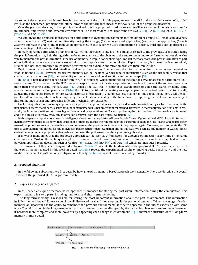
The long-term memory is responsible for storing the most important information about the past environments. This informationincludes the position and fitness value of the all discovered local and global optima in the past environments. Taking advantage of such amemory, an algorithm has the ability to remember the previous environments, if they re-appeared in the future exactly or with somenoise. The information in the long-term memory is persistent and does not disappear by the happening changes in environment. However,it becomes more complete and more powerful by happening each change in environment. Fig. 1 shows the structure of this long-termmemory in more detail.

Environment #1 Environment #2 Environment #3 …

Peak #1 Peak #2 Peak #3 …

Position Fitness value

Fig. 1. The structure of the long-term memory in detail.

B. Nasiri et al. / Neurocomputing 172 (2016) 356–370 357

The process of remembering the previous environments during the computation is as follows. At the beginning of each iteration, thesimilarity between current and previous environments is calculated using the modified Hausdorff Distance [49]

dðA;BÞ ¼ 1NðAÞ

X

aAA

dða;BÞ ð1Þ

dða;BÞ ¼MINbAB

dða; bÞ ð2Þ

dða; bÞ ¼ ‖a�b‖ ð3Þwhere d(A,B) is directed distance between two point sets of Environment A¼{a1,…, aN(A)} and B¼{b1,…, bN(B)}, d(a,B) is distance between apoint a and a set of points in Environment B¼{b1,…, bN(B)} and d(a,b) is the Euclidean distance between two points a and b. It is importantto mention that each point include the peak's position and its fitness as a dimension as well. If the distance between current and ithenvironment decreased sequentially more than M times (M is equal to 3 in this paper), we can say maybe a previous environments is re-appeared. Then the remembering process will be started by moving the GbestPosition of each peak in current environmentGbestPosEnvðcurÞPeakðiÞ Þ toward the GbestPosition of the nearest swarm of the most similar environment GbestPosEnvðMSEÞ

PeakðjÞ using Eq. (4). In thisalgorithm, rf is a parameter for adjusting the speed of remembering and in this paper we consider 0.5 for it

GbestPosEnvðcurÞPeakðiÞ ¼ GbestPosEnvðcurÞPeakðiÞ þrf nðGbestPosEnvðMSEÞPeakðjÞ �GbestPosEnvðcurÞPeakðiÞ Þ ð4Þ

The short-term memory is responsible for storing the all evaluated solution in current environment. It uses the Binary SpacePartitioning (BSP) tree structure for storing the valuable information. In this structure, the whole search space partition based on thedistribution of the individuals in the environment. Each node in this tree represents a unique hyper-rectangular box in the search spaceand contains a representative solution for this sub-area. Suppose a parent node has two child nodes. The sub-areas represented by thechild nodes are disjoint and their union is the sub-area of the parent. Fig. 2 shows the structure of the short-term memory which is used inthis paper.

Algorithm 1:. ShortTermMem_insertNode()

The process of adding a new solution to the short-term memory is shown in Algorithm 2. After each fitness evaluation, first, the short-term memory – BSP tree – must be traversed to find the sub-area which the new solution belongs to (cur_node). Then, the new solutionmust be compared with the representative solution of that sub-area (xcur_node) to find a cut-off point. The middle of the largest differencebetween the all dimensions of these two solutions (x and xcur_node) will be select as a cut-off point for creating two new child nodes. Formore detail on the BSP tree construction as well as a numerical example, please refer to [42].

Fig. 2. The structure of the each terminal and non-terminal node in short-term memory.

B. Nasiri et al. / Neurocomputing 172 (2016) 356–370358

HdPSO utilizes the short-term memory during the run (before each fitness evaluation) to decrease number of fitness evaluations bypredicting the fitness value of the solution using Algorithm 2.

Algorithm 2:. ShortTermMem_PredictSolution()

As we can see in this algorithm, the preliminary steps are completely similar to the Algorithm 1. The only difference is from line 11 to 15. Ifthe short-term memory is matured sufficiently, the algorithm will return the fitness value of the representative for the area which x isbelong to as a predicted value for solution x. The short-term memory is matured if the percentage of correct prediction is more than a pre-defined value (maturity_threshold). This percentage can be calculated after each fitness evaluation.

It is obvious that using this function for predicting the solutions in early stages of the run and before reaching enough maturity for the short-term memory can be harmful for the algorithm and in the opposite direction with the aim of using this function. That is why; one thresholdparameter – maturity_threshold – is defined for HdPSO to check the maturity of the short-term memory before using the predicted value.

2.2. History-Driven Particle Swarm Optimization (HdPSO)

In this section, a novel algorithm named History-Driven Particle Swarm Optimization (HdPSO) is proposed for optimization in dynamicenvironments. This algorithm utilizes the landscape historical information to improve its convergence speed, accuracy, and alsoremembering the previous environments if they re-appeared again in the future. Fig. 3 shows the block diagram of HdPSO and itsrelationship with the explicit memories.

Fig. 3. The block diagram of HdPSO with explicit memories.


Algorithm 3. Proposed Algorithm(HdPSO)

History-Driven Particle Swarm Optimization is a real coded swarm intelligence algorithm. For a D-dimensional landscape SCRD, a solutionx of HdPSO is a 1 by D real valued vector, i.e., xARD. This algorithm employs two different population – finder and tracker swarm – and alsotwo different explicit memories with vary structures to overcome the challenges which exist in dynamic environments. Among them, wecan mention to happening change in environment, transforming a local optima to a global one after a change in environment, losing theposition of the all optima after change, losing diversity in environment after change, outdated memory, converging two sub-swarms toone local optima and short interval of time between two change in environment. This work tries to introduce some mechanisms toovercome these challenges in dynamic optimization problem.

The proposed algorithm starts with initializing the finder and tracker swarms and also, short-term and long-term memories.Afterwards, change discovery, finder and tracker swarm processing and also fine tuning process are repeated until the number of fitnessevaluations exceeds a pre-determined value. Algorithm 3 shows the block diagram of the HdPSO. In the following, each step in thisalgorithm is described in detail.

Algorithm 4:. Initialization()

The initialization process is shown in Algorithm 4. The algorithm consists of two different types of swarms including finder and trackerswarms. The finder swarm is configured somehow to explore the new promising areas in the search space effectively and efficiently. Oncethe finder swarm converged to a local optima, the k-best particles in it should be considered as a new tracker swarm, and the finderswarm should be re-initialized. The tracker swarm is responsible for chasing the discovered optima in the environment and does not have


any particle initially. Also, the short-term memory initialized by adding a single node which is the root node of the BSP tree. However, thelong-term memory has not any entry at the first.

At the first step in the main loop of the algorithm, the previous environment remembering process will happen. The detail of this stepis provided in the previous section completely.

As noted in the introduction part, there are two methods for discovering change in dynamic environment, including re-evaluating apre-specified test solution, and monitoring behavioral change in algorithm during the run. The current work presents a hybrid approachbased on two mentioned methods for discovering change in environment as shown in Algorithm 5. In this algorithm first, the trend of aperformance KPI should be checked during k-latest fitness evaluations. This KPI is the mean of all fitness evaluations after the latestchange in environment. If the trend of this KPI is increasing, the algorithm needs to re-evaluate the pre-specified test solution for ensuringabout happening change in environment. This hybrid approach can help the algorithm to decrease the number of wasted fitnessevaluation for discovering change in environment. In this work, we used 4 for the k value.

Algorithm 5. Change_discovery()

After the change is discovered in the environment, two actions should be done in environment. First, all discovered optima should beadded to the long-term memory and then all the particles in each tracker swarm should be diversified. This diversification can be done byadding a random value in range of [�VlengthnP, VlengthnP] to the GbestPosition of each tracker swarm.

Env1 Envi

EnvPL

……

Fig. 4. Pendulum motion of environments.


Algorithm 6. Swarm_Moving()

After the change discovery, the algorithm will start a finder swarm process if this swarm is active in environment. The finder swarmprocess includes three actions including swarm moving, exclusion and convergence checking.

The swarm moving, as shown in Algorithm 6, is very similar to the standard particle swarm optimization with some minor changes asbelow:

1) The fitness value of the each particle should be predicted by the BSP tree before actual fitness evaluation. If the predicted value for thisnew position is equal or better than its Pbest fitness value, the actual fitness evaluation will be happen on new position of the particle.

2) The position of each particle will change if the fitness value of the new position is better than current position.

Also, the exclusion and convergence checking algorithms are shown in Algorithm 7,8. In Exclusion algorithm, the finder swarm will bere-initialized if the distance between the Gbest of each swarm and finder swarm or any other tracker swarm is less than rexcl.

Algorithm 7. exclusion()

Algorithm 8. finderConvergenceChecking()


Based on Algorithm 8, the finder swarm is converged if the difference between the fitness value of the best global particle during the lasttwo iterations is less than rconv or the distance between the best global particle during the last two iterations is less than rconv/5. After theconvergence of finder swarm, the m best particle in it will move to the tracker swarm and the finder swarm will be re-initialized.

After the finder swarm process, the tracker swarm will start by swarm moving, swarm freezing and fine-tuning process. The swarmmoving for the tracker swarm uses the same algorithm as finder swarm (Algorithm 6).

The swarm freezing, as shown in Algorithm 9, is an action which used for freezing the tracker swarms which have not any influence inimprovement of the algorithm's result. In this way, the algorithm does not waste the fitness evaluations to improve some particles whichhave not any influence on performance of the whole algorithm. A tracker swarmwill be freeze if its Gbestposition or fitness did not changeconsiderably during their last three iterations.

Algorithm 9. Swarm_freezing()

Algorithm 10. Fine-tuning()

The aim of fine-tuning algorithm (Algorithm 10) is to improve the overall result of the algorithm as much as possible. That is why thisalgorithm tries to enhance the quality of global best particle in environment by doing some local search around it. Predicting newsolutions after each movement can help the algorithm to reduce the number of wasted fitness evaluation during this phase. New positioncan be achieved by using the following equation:

xnew ¼ Gbest_positionþðrcloud � RjÞ ð5Þwhere Rj is a random number with uniform distribution in [�1, 1]. Hence, the xnew is located in the radius of rcloud from Gbest. Also, rcloudwill decrease based on Eq. (6)

rcloud ¼ rcloud � ðwminþðrand� ðwmax�wminÞÞ ð6Þwhere Wmin, Wmax are the lower and the upper bounds for multiplying in rcloud.

3. Experimental study

3.1. Benchmark problems

Due to time consuming evaluations of fitness functions in the real-world problems, the computation cost of an algorithm in mostapplications is expressed in terms of the number of evaluations; as is done in this paper. The first benchmark used in this paper is theMoving Peaks Benchmark (MPB) [4,50], which is the most commonly used benchmark for evaluating algorithms in dynamic environments[51]. The reason for this popularity amongst the researchers is related to the large number of adjustable parameters in this benchmark forgenerating a wide range of dynamic environments. Using this benchmark, we can study algorithms from a number of perspectives.

In MPB, there are a number of peaks in a D-dimensional space which their widths, heights and positions will change by a fixed amounts (shift severity), every α fitness evaluation. The goal of the problem is to locate and track the global peak (optima) in environment duringthe all changes which happen to environment over the time. More detail about MPB, can be fined in [4].

The second benchmark used in this paper, is a modified version of MPB with pendulum motion characteristic (Fig. 4), namelyPendulum-MPB (PMPB). In fact, most of the dynamic optimization algorithms that enhanced with memory are expected to work better on


environments that re-appear in the future. In this benchmark, pendulum length (PL) parameter is introduced to control the linearpendulum motion accurately and correctly.

Algorithm 11. Environment_selector()

The implementation for PMPB is as follows. For the first PL changes in environments, the whole peak positions should be stored in an arraymemory for the future use. Afterwards, for every change in the environment, the position of the peaks should be achieved from the nextenvironment returned from Algorithm 11. It should be mentioned that the first value for the direction parameter should be set to right.

3.2. Performance metric

There are several performance metrics used in the literature to measure the efficiency of optimization algorithm in dynamicenvironments [52]. In order to make our results comparable with other state-of-the-art algorithms, the metric selected in this paper is theoffline error (OE) which is the average of the differences between the values found so far by the algorithm and the global optimum value[4,50].

OE ¼ 1FE

XFE

t ¼ 1f gbest tð Þð Þ� f globalOptimum tð Þð Þð Þ ð7Þ

where FEs is the total number of fitness evaluations, and globalOptimum(t) and gbest(t) are the global optimum value and the best valuefound by the algorithm at the t-th fitness evaluation, respectively. It is worth mentioning that in[8,9], offline error is calculated usingdifferent approach, in which instead of using the average of current errors in all fitness evaluations, average of current errors before eachenvironment change is utilized. In this paper, we calculate offline error based on Eq. (7) for comparing the algorithms' results.

Table 1MPB parameters setting.

Parameter Value

Number of peaks, M Variable between 1 and 200Change frequency, α 500, 1000, 2500, 5000, 10000Height change 7.0Width change 1.0Peaks shape ConeBasic function NoChange severity, s 1, 2, 3, 5Number of dimensions, D 5Correlation Coefficient, λ 0Peaks location range [0–100]Peak height [30.0–70.0]Peak width [1–12]Initial value of peaks 50.0


3.3. Parameters setting

In this section, the required parameters setting for the algorithm is provided. For the MPB, the parameters are set according to scenario2 of this benchmark [4] in Table 1. However, in order to study the various aspects of the algorithm for some important parameters such asnumber of peaks, change frequency, dimensions, and change severity, several values are specified in this table.

In addition, for the PMPB problem, the PL parameter is set to 5, 10 and 20. It means that the environments will re-appear in pendulummanner after 5, 10 and 20 changes in the environment.

Also, based on the default configuration of MPB (M¼10, α¼5000, s¼1), some preliminary experiments are conducted to achieve thebest values for the parameters of HdPSO. The obtained preliminary results are presented in Fig. 5.

So, the initial configuration of the proposed algorithm is achieved based on the best combination of the parameters as follows (Table 2).Also, the rexcl and rconv parameters are considered according to [12].

3.4. Comparison between HdPSO and other state of art methods

In this part, the efficiency and performance of HdPSO is tested on different MPB configurations and is compared with several state-of-the-art algorithms. The experimental results are obtained by the average of 50 executions of algorithm. Also, in each of them, the initialposition of the particles and the peaks are determined randomly and with different random seeds. Termination condition of the allalgorithms is 100 changes in environment which is equal to 100 n α fitness evaluation. Some of the presented results of the state-of-artalgorithms are obtained by implementing the methods and some of them are extracted from the related references. In Tables 3–7, theefficiency of sixteen related algorithms including: mQSO [12], AmQSO [53], mPSO [54], HmPSO [55] APSO [56], FTMPSO [57], CESO [58],mNAFSA [59], PSO-AQ [60], CDEPSO [61], CellularDE [21], SFA [62], DynPopDE [25], MLDE-S [20], CbDE-wCA [23] and DPSABC [34] iscompared with that of HdPSO. All simulations are performed on a PC with 2.8 GHz CPU and 8 GB memory. Also, the proposed algorithm isimplemented in MATLAB language version 2012. Furthermore, for each environment, t-test with a significance level of 0.05 has beenapplied and the result of the best performing algorithms is printed in bold. When the results for the best performing algorithms are notsignificantly different, all are printed in bold.

Fig. 5. Preliminary result for different parameters setting.

Table 2HdPSO parameters setting.

Parameter Value

Number of particles in finder swarm 10Number of particles in tracker swarm 5P 0.5Wmin 0.6Wmax 0.9rcloud 0.2ns (change severity)


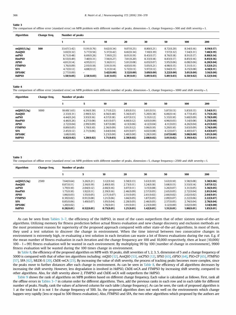
As can be seen from Tables 3–7, the efficiency of the HdPSO, in most of the cases outperform that of other sixteen state-of-the-artalgorithms. Utilizing memory for fitness prediction before actual fitness evaluation and new change discovery and exclusion methods arethe most prominent reasons for superiority of the proposed approach compared with other state-of-the-art algorithms. In most of them,they used a test solution to discover the change in environment. When the time interval between two consecutive changes inenvironment is extremely high, re-evaluating a test solution in each iteration can waste a lot of fitness evaluations during the run. E.g. ifthe mean number of fitness evaluation in each iteration and the change frequency are 100 and 10,000 respectively, then at least (10,000/100�1¼99) fitness evaluation will be wasted in each environment. By multiplying 99 by 100 (number of change in environment), 9900fitness evaluation will be wasted during the 100 times change in environment.

In Table 8, the efficiency of the proposed algorithm onMPBwith 10 peaks, shift severities of 1, 2, 3, 5, dimension of 5 and a change frequency of5000 is compared with that of other ten algorithms including: mQSO [12], AmQSO [53], mCPSO [12], SPSO [63], rSPSO [64], PSO-CP [65], FTMPSO[57], SFA [62], MLDE-S [20], CbDE-wCA [23]. By increasing the value of shift severity, the process of tracking peaks becomes more complex, sincethe peaks move to further distances after each change in environment. As can be seen in Table 8, the efficiency of all algorithms decreases byincreasing the shift severity. However, less degradation is involved in HdPSO, CbDE-wCA and FTMPSO by increasing shift severity, compared toother algorithms. Also, for shift severity above 2, FTMPSO and CbDE-wCA will outperform the HdPSO.

Table 9 shows the rank of algorithms on MPB problem based on different change frequency. Each value is calculated as follows. First, rank allthe offline errors in Tables 3–7 in column order for different algorithms. Then, add the previous ranks in each row and in each table for differentnumber of peaks. Finally, rank the values of achieved column for each table (change frequency). As can be seen, the rank of proposed algorithm is1 at the total but it is not 1 for change frequency of 500. So, the proposed algorithm does not work well on the environments which changehappen very rapidly (less or equal to 500 fitness evaluation). Also, FTMPSO and SFA, the two other algorithms which proposed by the authors are

Table 3The comparison of offline error (standard error) on MPB problem with different number of peaks, dimension¼5, change frequency¼500 and shift severity¼1.

Algorithm Change freq. Number of peaks

1 5 10 20 30 50 100 200

mQSO(5,5q) 500 33.67(3.42) 11.91(0.76) 9.62(0.34) 9.07(0.25) 8.80(0.21) 8.72(0.20) 8.54(0.16) 8.19(0.17)AmQSO 3.02(0.32) 5.77(0.56) 5.37(0.42) 6.82(0.34) 7.10(0.39) 7.57(0.32) 7.34(0.31) 7.48(0.19)mPSO 8.71(0.48) 6.69(0.26) 7.19(0.23) 8.01(0.19) 8.43(0.17) 8.76(0.18) 8.91(0.17) 8.88(0.14)HmPSO 8.53(0.49) 7.40(0.31) 7.56(0.27) 7.81(0.20) 8.33(0.18) 8.83(0.17) 8.85(0.16) 8.85(0.16)APSO 4.81(0.14) 4.95(0.11) 5.16(0.11) 5.81(0.08) 6.03(0.07) 5.95(0.06) 6.08(0.06) 6.20(0.04)FTMPSO 1.76(0.09) 2.93(0.18) 3.91(0.19) 4.83(0.19) 5.05(0.21) 4.98(0.15) 5.31(0.11) 5.52(0.21)SFA 4.72(0.12) 4.88(0.12) 5.11(0.14) 5.72(0.13) 5.97(0.12) 5.94(0.15) 6.15(0.08) 6.18(0.11)DPSABC 2.77(0.00) – 3.42(0.00) 3.12(0.00) 3.69(0.00) 3.22(0.00) 3.01(0.00) 3.16(0.00)HdPSO 1.50(0.05) 2.58(0.03) 3.41(0.03) 4.39(0.01) 5.09(0.03) 5.89(0.03) 6.50(0.02) 6.32(0.04)



1 5 10 20 30 50 100 200

mQSO(5,5q) 2500 7.64(0.64) 3.26(0.21) 3.12(0.14) 3.58(0.13) 3.63(0.10) 3.63(0.10) 3.58(0.08) 3.30(0.06)AmQSO 0.87(0.11) 2.16(0.19) 2.49(0.10) 2.73(0.11) 3.24(0.18) 3.68(0.15) 3.53(0.14) 3.07(0.12)mPSO 1.79(0.10) 2.04(0.12) 2.66(0.16) 3.07(0.11) 3.15(0.08) 3.26(0.07) 3.31(0.05) 3.36(0.05)HmPSO 1.75(0.10) 1.92(0.11) 2.39(0.16) 2.46(0.09) 2.57(0.05) 2.65(0.05) 2.72(0.04) 2.81(0.04)APSO 1.06(0.03) 1.55(0.05) 2.17((0.07) 2.51(0.05) 2.61(0.02) 2.66(0.02) 2.62(0.02) 2.64(0.01)FTMPSO 0.39(0.02) 0.91(0.08) 1.21(0.06) 1.66(0.05) 1.87(0.05) 2.09(0.07) 2.22(0.06) 2.22(0.07)SFA 0.85(0.06) 1.49(0.07) 1.95(0.04) 2.28(0.05) 2.46(0.05) 2.57(0.05) 2.74(0.04) 2.76(0.04)DPSABC 1.20(0.02) – 1.76(0.01) 1.91(0.01) 2.23(0.00) 3.12(0.00) 3.02(0.00) 3.14(0.00)HdPSO 0.28(0.01) 0.52(0.01) 0.75(0.01) 1.21(0.01) 1.42(0.01) 1.51(0.01) 1.80(0.01) 1.85(0.01)



1 5 10 20 30 50 100 200

mQSO(5,5q) 1000 18.60(1.63) 6.56(0.38) 5.71(0.22) 5.85(0.15) 5.81(0.15) 5.87(0.13) 5.83(0.13) 5.54(0.11)AmQSO 2.33(0.31) 2.90(0.32) 4.56(0.40) 5.36(0.47) 5.20(0.38) 6.06(0.14) 4.77(0.45) 5.75(0.26)mPSO 4.44(0.24) 3.93(0.16) 4.57(0.18) 4.97(0.13) 5.15(0.12) 5.33(0.10) 5.60(0.09) 5.78(0.09)HmPSO 4.46(0.26) 4.27(0.08) 4.61(0.07) 4.66(0.12) 4.83(0.09) 4.96(0.03) 5.14(0.08) 5.25(0.08)APSO 2.72(0.04) 2.99(0.09) 3.87(0.08) 4.13(0.06) 4.12(0.04) 4.11(0.03) 4.26(0.04) 4.21(0.02)FTMPSO 0.89(0.05) 1.70(0.10) 2.36(0.09) 3.01(0.12) 3.06(0.10) 3.29(0.10) 3.63(0.09) 3.74(0.09)SFA 2.45(0.12) 2.71(0.06) 3.64(0.04) 4.01(0.07) 4.02(0.08) 4.12(0.07) 4.40(0.07) 4.43(0.07)DPSABC 1.68(0.00) – 3.23(0.00) 3.40(0.00) 3.28(0.00) 2.67(0.00) 3.08(0.00) 3.01(0.00)HdPSO 0.82(0.02) 1.20(0.02) 1.71(0.03) 2.38(0.02) 2.88(0.02) 3.01(0.02) 3.39(0.02) 3.57(0.01)


in the second and third place in this ranking which proposed by the authors recently. It is worth mentioning that CbDE-wCA does not included inthis table because the result in its paper is only available for change frequency of 5000. However, from Tables 6 and 8, it seems that this algorithmcan outperform the proposed approach on some specific configuration such as high shift severity.

3.5. Comparison of HDPSO on PMPB problem

In this section, the performance of the proposed algorithm is evaluated on Pendulum-MPB (PMPB) problem. This benchmark is defined for thefirst time in this paper and is described in Section 3.1 completely. As we said before, the PL parameter is set to 5, 10 and 20. It means that theenvironments will re-appear in pendulum manner after 5, 10 and 20 changes in an environment. Table 9 shows the performance of HdPSO onMPB and PMPB. As we can see in Table 10, the more the pendulum length parameter increases, the more the efficiency of the algorithm decreases.

Table 7The comparison of offline error (standard error) on MPB problem with different number of peaks, dimension¼5, change frequency¼10,000 and shift severity¼1.


1 5 10 20 30 50 100 200

mQSO(5,5q) 10,000 1.90(0.18) 1.03(0.06) 1.10(0.07) 1.84(0.08) 2.00(0.09) 1.99(0.07) 1.85(0.05) 1.71(0.04)AmQSO 0.19(0.02) 0.45(0.04) 0.76(0.06) 1.28(0.12) 1.78(0.09) 1.55(0.08) 1.89(0.14) 2.52(0.10)mPSO 0.27(0.02) 0.70(0.10) 0.97(0.04) 1.34(0.08) 1.43(0.05) 1.47(0.04) 1.50(0.03) 1.48(0.02)APSO 0.25(0.01) 0.57(0.03) 0.82(0.02) 1.23(0.02) 1.39(0.02) 1.46(0.01) 1.38(0.01) 1.36(0.01)FTMPSO 0.09(0.00) 0.31(0.04) 0.43(0.03) 0.56(0.01) 0.69(0.09) 0.86(0.02) 1.08(0.03) 1.13(0.04)SFA 0.26(0.03) 0.53(0.04) 0.72(0.02) 0.91(0.03) 0.99(0.04) 1.19(0.04) 1.44(0.04) 1.52(0.03)DPSABC 2.67(0.00) – 9.00(0.01) 6.60(0.01) 7.70(0.01) 8.10(0.01) 8.34(0.01) 8.52(0.01)HdPSO 0.06(0.00) 0.25(0.01) 0.29(0.01) 0.38(0.00) 0.57(0.00) 0.73(0.00) 0.84(0.00) 0.97(0.01)



1 5 10 20 30 50 100 200

mQSO(5,5q) 5000 2.24(0.05) 1.82(0.08) 1.85(0.08) 2.48(0.09) 2.51(0.10) 2.53(0.08) 2.35(0.06) 2.24(0.05)AmQSO 2.62(0.10) 1.01(0.09) 1.51(0.10) 2.00(0.15) 2.19(0.17) 2.43(0.13) 2.68(0.12) 2.62(0.10)mPSO 2.24(0.05) 1.82(0.08) 1.85(0.08) 2.48(0.09) 2.51(0.10) 2.53(0.08) 2.35(0.06) 2.24(0.05)HmPSO 2.62(0.10) 1.01(0.09) 1.51(0.10) 2.00(0.15) 2.19(0.17) 2.43(0.13) 2.68(0.12) 2.62(0.10)APSO 0.53(0.01) 1.05(0.06) 1.31(0.03) 1.69(0.05) 1.78(0.02) 1.95(0.02) 1.95(0.01) 1.90(0.01)FTMPSO 0.18(0.01) 0.47(0.05) 0.67(0.04) 0.93(0.04) 1.14(0.04) 1.32(0.04) 1.61(0.03) 1.67(0.03)SFA 0.42(0.03) 0.89(0.07) 1.05(0.04) 1.48(0.05) 1.56(0.06) 1.87(0.05) 2.01(0.04) 1.99(0.06)CESO 1.04(0.00) – 1.38(0.02) 1.72(002) 1.24(0.01) 1.45(0.01) 1.28(0.02) –

mNAFSA 0.59(0.06) 0.66(0.05) 0.94(0.04) 1.29(0.05) 1.60(0.06) 1.81(0.06) 1.92(0.05) 1.97(0.05)PSO-AQ 0.34(0.02) 0.80(0.12) 0.89(0.03) 1.45(0.06) 1.52(0.04) 1.77(0.05) 1.95(0.05) 1.96(0.04)CDEPSO 0.41(0.00) 0.97(0.01) 1.22(0.01) 1.54(0.01) 2.62(0.01) 2.20(0.01) 1.54(0.01) 2.11(0.01)CellularDE 1.53(0.07) 1.50(0.04) 1.64(0.03) 2.46(0.05) 2.62(0.05) 2.75(0.05) 2.73(0.03) 2.61(0.02)DynPopDE – 1.03(0.13) 1.39(0.07) – – 2.10(0.06) 2.34(0.05) 2.44(0.05)MLDE-S 1.11(0.07) – 1.35(0.07) – – – 1.65(0.08) –

CbDE-wCA 0.14(0.03) 0.30(0.02) 0.86(0.08) 0.98(0.05) 1.34(0.04) 1.31(0.04) 1.35(0.03) 1.29(0.02)DPSABC 2.25(0.00) 2.13(0.00) 2.07(0.00) 1.88(0.00) 1.91(0.00) 1.89(0.00) 1.87(0.00)HdPSO 0.16(0.01) 0.34(0.01) 0.49(0.01) 0.68(0.01) 0.83(0.01) 1.08(0.01) 1.15(0.01) 1.18(0.01)

Table 8The comparison of offline error (standard error) on MPB problem with different shift severities, dimension¼5, peak number¼10, change frequency¼5000.

Algorithm Shift severity

1 2 3 5

mQSO(5,5q) 1.85(0.08) 2.40(0.06) 3.00(0.06) 4.24(0.10)AmQSO 1.51(0.10) 2.09(0.08) 2.72(0.09) 3.71(0.11)mCPSO 4.89(0.11) 3.57(0.08) 2.80(0.07) 2.08(0.07)SPSO 2.51(0.09) 3.78(0.09) 4.96(0.12) 6.76(0.15)rSPSO 1.50(0.08) 1.87(0.05) 2.40(0.08) 3.25(0.09)PSO-CP 1.31(0.06) 1.98(0.06) 2.21(0.06) 3.20(0.13)FTMPSO 0.67(0.04) 1.20(0.06) 1.40(0.09) 1.69(0.07)SFA 1.05(0.04) 1.44(0.06) 2.06(0.07) 2.89(0.13)MLDE-S 1.35(0.07) 1.91((0.08) 2.34(0.07) 2.68(0.11)CbDE-wCA 0.86(0.08) 0.88(0.08) 0.98(0.09) 1.54(0.7)HdPSO 0.49(0.01) 0.78(0.01) 1.48(0.03) 1.98(0.02)


4. Conclusion

In this paper, a novel optimization algorithm with and explicit memory was proposed for working on dynamic environments. Theproposed algorithm could quickly find the peaks in the problem space and follow them after an environment change. Also, it could utilizethe previous history of the search space to guide the search to the promising area and avoid wasting fitness area. In the proposedalgorithm, swarms in the problem space were categorized into finder and tracker swarms which were configured somehow to completeeach other during the search process.

Efficiency of the proposed algorithm has been evaluated on moving peaks benchmark, which is the most well-known benchmark inthis domain, and a modified version of it, called PMPB. The results were compared with those of the state-of-the-art algorithms. Theexperimental results and comparative studies showed the superiority of the proposed algorithm. Diverse experiments showed that theproposed algorithm involved a high convergence speed which is significantly important in designing any optimization algorithm indynamic environments. Each swarm has been equipped with some mechanisms, based on its corresponding function, to conquer itsparticular challenges. As a result, the functions of swarms were appropriately performed.

We would like to apply the proposed methods as a boosting technique to some powerful optimization algorithms such as CoBiDE [45],CoDE [46], BSA [47] and DSA [48] instead of PSO. Also, we would like to use the proposed algorithm on different dynamic benchmarkproblems and also real applications. Currently, we are working on its applications to the clustering in web, and to the personalization ofweb pages dynamically. Adapting the algorithm to dynamic multi-objective optimization is one of the goals that will be pursued in nearfuture. Also, we are working to make adaptive the important parameters in HdPSO for easier to use.

References

[1] T.T. Nguyen, S. Yang, J. Branke, Evolutionary dynamic optimization: a survey of the state of the art, Swarm Evolut. Comput. 6 (2012) 1–24.[2] T.T. Nguyen, Continuous dynamic optimisation using evolutionary algorithms, PhD. Thesis, University of Birmingham, 2011.[3] C. Li, S. Yang, M. Yang, An adaptive multi-swarm optimizer for dynamic optimization problems, Evol. Comput. 22 (4) (2014) 1–36.[4] J. Branke. (1999). The Moving Peaks Benchmark. Available: ⟨http://web.archive.org/web/20130906140931/http:/people.aifb.kit.edu/jbr/MovPeaks/⟩.[5] R.W. Morrison and K.A. De Jong, A test problem generator for non-stationary environments, In: Proceedings of the IEEE Congress on Evolutionary Computation, CEC

1999, 1999, pp. 2053.[6] S. Yang, Non-stationary problem optimization using the primal-dual genetic algorithm In: Proceedings of the 2003 Congress on Evolutionary Computation, CEC 2003,

2003, pp. 2246–2253.[7] C. Li and S. Yang, A clustering particle swarm optimizer for dynamic optimization, In: Proceedings of the IEEE Congress on Evolutionary Computation, CEC, 2009,

pp. 439–446.[8] S. Yang, C. Li, A clustering particle swarm optimizer for locating and tracking multiple optima in dynamic environments, IEEE Trans. Evolut. Comput. 14 (2010) 959–974.[9] C. Li, S. Yang, A general framework of multi-population methods with clustering in undetectable dynamic environments, IEEE Trans. Evolut. Comput. 16 (2011) 556–577.[10] J. Branke, H. Schmeck, Designing evolutionary algorithms for dynamic optimization problems, Adv. Evolut. Comput.: Theory Appl. (2002) 239–262.[11] T. Blackwell, J. Branke, Multi-swarm optimization in dynamic environments, Appl. Evolut. Comput. 3005 (2004) 489–500.[12] T. Blackwell, J. Branke, Multiswarms, exclusion, and anti-convergence in dynamic environments, IEEE Trans. Evolut. Comput. 10 (2006) 459–472.[13] X. Li, J. Branke, and T. Blackwell, Particle swarmwith speciation and adaptation in a dynamic environment, in: Proceedings of the 8th Annual Conference on Genetic and

Evolutionary Computation, 2006, pp. 51–58.[14] F. Oppacher and M. Wineberg, The shifting balance genetic algorithm: improving the GA in a dynamic environment in: Proceedings of the Genetic and Evolutionary

Computation Conference, GECCO, 1999, pp. 504–510.[15] W. Rand, R. Riolo, and J.H. Holland, The effect of crossover on the behavior of the GA in dynamic environments: a case study using the shaky ladder hyperplane-defined

functions, in: Proceedings of the 8th Annual Conference on Genetic and Evolutionary Computation (GECCO 2006), 2006, pp. 1289–1296.[16] H.C. Andersen, An Investigation into Genetic Algorithms, and the Relationship between Speciation and the Tracking of Optima in Dynamic Functions, Honors,

Queensland University, Brisbane, Australia, 1991.[17] X. Wang, X.Z. Gao, and S.J. Ovaska, An immune-based ant colony algorithm for static and dynamic optimization, in: Proceedings of the IEEE International Conference on

Systems, Man and Cybernetics, 2007, pp. 1249–1255.

Table 10comparison of offline error (standard error) on PMPB and MPB problems with different number of peaks, dimension¼5, change frequency¼5000 and shift severity¼1.

Algorithm Problem Number of peaks

1 5 10 20 30 50 100 200

HdPSO MPB 0.14(0.00) 0.30(0.01) 0.51(0.01) 0.70(0.01) 0.88(0.01) 1.17(0.01) 1.23(0.01) 1.26(0.01)HdPSO PMPB l¼5 0.05(0.00) 0.10(0.01) 0.20(0.01) 0.26(0.01) 0.32(0.01) 0.37(0.01) 0.41(0.01) 0.43(0.01)HdPSO PMPB l¼10 0.07(0.00) 0.14(0.01) 0.25(0.01) 0.36(0.01) 0.42(0.01) 0.53(0.01) 0.63(0.01) 0.63(0.01)HdPSO PMPB l¼20 0.10(0.00) 0.23(0.01) 0.33(0.01) 0.53(0.01) 0.60(0.01) 0.70(0.01) 0.80(0.01) 0.88(0.01)

Table 9The rank of algorithms on MPB problem based on different change frequenc.

Algorithm Change frequency

500 1000 2500 5000 10,000 Overall ranking

mQSO(5,5q) 9 8 9 8 7 9AmQSO 6 5 7 7 5 6mPSO 8 7 8 8 6 8HmPSO 7 6 6 7 8 7APSO 5 4 5 5 4 5FTMPSO 2 2 3 3 2 2SFA 4 3 4 4 3 3DPSABC 1 2 2 6 9 4HdPSO 3 1 1 1 1 1


http://refhub.elsevier.com/S0925-2312(15)01046-2/sbref1



http://web.archive.org/web/20130906140931/http:/people.aifb.kit.edu/jbr/MovPeaks/








[18] M. Mavrovouniotis and S. Yang, Ant colony optimization algorithms with immigrants schemes for the dynamic travelling salesman problem, in: EvolutionaryComputation for Dynamic Optimization Problems, Shengxiang Yang, Xin Yao 2011, pp. 317–341.

[19] M. Mavrovouniotis, S. Yang, Dynamic Vehicle Routing: A Memetic Ant Colony Optimization Approach, in: A.S. Uyar, E. Ozcan, N. Urquhart (Eds.), Automated Schedulingand Planning. vol. 505, Springer, Berlin Heidelberg, 2013, pp. 283–301.

[20] S. Kundu, D. Basu, S. Chaudhuri, Multipopulation-Based Differential Evolution with Speciation-Based Response to Dynamic Environments, in: B. Panigrahi, P. Suganthan,S. Das, S. Dash (Eds.), Swarm, Evolutionary, and Memetic Computing. vol. 8297, Springer International Publishing, 2013, pp. 222–235.

[21] V. Noroozi, A. Hashemi, and M. Meybodi, CellularDE: a cellular based differential evolution for dynamic optimization problems, Adaptive and Natural ComputingAlgorithms, 2011, pp. 340–349.

[22] U. Halder, S. Das, D. Maity, A cluster-based differential evolution algorithm with external archive for optimization in dynamic environments, Cybern. IEEE Trans. 43(2013) 881–897.

[23] R. Mukherjee, G.R. Patra, R. Kundu, S. Das, Cluster-based differential evolution with Crowding Archive for niching in dynamic environments, Inf. Sci. 267 (2014) 58–82.[24] J. Brest, P. Korošec, J. Šilc, A. Zamuda, B. Bošković, M.S. Maučec, Differential evolution and differential ant-stigmergy on dynamic optimisation problems, Int. J. Syst. Sci.

44 (2013) 663–679.[25] M.C. du Plessis, A.P. Engelbrecht, Differential evolution for dynamic environments with unknown numbers of optima, J. Glob. Optim. 55 (2013) 73–99.[26] J. Brest, A. Zamuda, B. Boskovic, M.S. Maucec, and V. Zumer, Dynamic optimization using self-adaptive differential evolution In: Proceedings of the IEEE Congress on

Evolutionary Computation, 2009, pp. 415–422.[27] R. Mendes and A.S. Mohais, DynDE: a differential evolution for dynamic optimization problems, In: Proceedings of the 2005 IEEE Congress on Evolutionary

Computation, 2005, pp. 2808–2815.[28] M.C. du Plessis and A.P. Engelbrecht, Improved Differential Evolution for Dynamic Optimization Problems, 2008, pp. 229–234.[29] W. Shuzhen, X. Shengwu, and L. Yi, Prediction based multi-strategy differential evolution algorithm for dynamic environments, In: Proceedings of the 2012 IEEE

Congress on Evolutionary Computation (CEC), 2012, pp. 1–8.[30] M.C. du Plessis, A.P. Engelbrecht, Using competitive population evaluation in a differential evolution algorithm for dynamic environments, Eur. J. Oper. Res. 218 (2012) 7–20.[31] S. Biswas, S. Kundu, S. Das, and A. Vasilakos, Information sharing in bee colony for detecting multiple niches in non-stationary environments, in: Proceedings of the 15th

Annual Conference Companion on Genetic and Evolutionary Computation, 2013, pp. 1–2.[32] S. Raziuddin, S.A. Sattar, R. Lakshmi, M. Parvez, Differential artificial bee colony for dynamic environment, Adv. Comput. Sci. Inf. Technol. 131 (2011) 59–69.[33] S. Raziuddin, S. Sattar, R. Lakshmi, M. Parvez, Differential Artificial Bee Colony for Dynamic Environment, in: N. Meghanathan, B. Kaushik, D. Nagamalai (Eds.), Advances

in Computer Science and Information Technology. vol. 131, Springer, Berlin Heidelberg, 2011, pp. 59–69.[34] N. Baktash, M.R. Meybodi, A new hybrid model of PSO and ABC algorithms for optimization in dynamic environment, Int. J. Comput. Theory Eng. 4 (2012) 362–364.[35] N. Baktash, F. Mahmoudi, M.R. Meybodi, Cellular PSO-ABC: a new hybrid model for dynamic environment, Int. J. Comput. Theory Eng. 4 (2012) 365–368.[36] S. Biswas, D. Bose, S. Kundu, A Clustering Particle Based Artificial Bee Colony Algorithm for Dynamic Environment, in: B. Panigrahi, S. Das, P. Suganthan, P. Nanda (Eds.),

Swarm, Evolutionary, and Memetic Computing. vol. 7677, Springer, Berlin Heidelberg, 2012, pp. 151–159.[37] S. Yang, X. Yao, Population-based incremental learning with associative memory for dynamic environments, IEEE Trans. Evolut. Comput. 12 (2008) 542–561.[38] E.L. Yu and P.N. Suganthan, Evolutionary programming with ensemble of explicit memories for dynamic optimization, In: Proceedings of the IEEE Congress on

Evolutionary Computation, CEC, 2009, pp. 431–438.[39] H. Richter, S. Yang, Memory Based on Abstraction for Dynamic Fitness Functions, in: M. Giacobini, A. Brabazon, S. Cagnoni, G. Di Caro, R. Drechsler, A. Ekárt, et al., (Eds.),

in Applications of Evolutionary Computing. vol. 4974, Springer, Berlin Heidelberg, 2008, pp. 596–605.[40] S.Y. Yuen and C.K. Chow, A non-revisiting genetic algorithm, In: Proceedings of the IEEE Congress on Evolutionary Computation, CEC 2007, 2007, pp. 4583–4590.[41] S.Y. Yuen, C.K. Chow, A genetic algorithm that adaptively mutates and never revisits, IEEE Trans. Evolut. Comput. 13 (2009) 454–472.[42] C.K. Chow, S.Y. Yuen, An evolutionary algorithm that makes decision based on the entire previous search history, IEEE Trans. Evolut. Comput. 15 (2011) 741–769.[43] S.W. Leung, S.Y. Yuen, C.K. Chow, Parameter control system of evolutionary algorithm that is aided by the entire search history, Appl. Soft Comput. 12 (2012) 3063–3078.[44] S.W. Leung, S.Y. Yuen, and C.K. Chow, Parameter control by the entire search history: case study of history-driven evolutionary algorithm In: Proceedings of the IEEE

Congress on Evolutionary Computation, CEC 2010, 2010, pp. 1–8.[45] Y. Wang, H.-X. Li, T. Huang, L. Li, Differential evolution based on covariance matrix learning and bimodal distribution parameter setting, Appl. Soft Comput. 18 (2014) 232–247.[46] Y. Wang, Z. Cai, Q. Zhang, Differential evolution with composite trial vector generation strategies and control parameters, Evolut. Comput. IEEE Trans. 15 (2011) 55–66.[47] P. Civicioglu, Backtracking search optimization algorithm for numerical optimization problems, Appl. Math. Comput. 219 (2013) 8121–8144.[48] P. Civicioglu, Transforming geocentric cartesian coordinates to geodetic coordinates by using differential search algorithm, Comput. Geosci. 46 (2012) 229–247.[49] M.P. Dubuisson and A.K. Jain, A modified Hausdorff distance for object matching, in: Proceedings of the 12th IAPR International Conference on Pattern Recognition, Vol.

1-Conference A: Computer Vision & Image Processing, 1994, pp. 566–568.[50] J. Branke, Memory enhanced evolutionary algorithms for changing optimization problems, In: Proceedings of the IEEE Congress on Evolutionary Computation, CEC, 1999.[51] J. Yaochu, J. Branke, Evolutionary optimization in uncertain environments – a survey, IEEE Trans. Evolut. Comput. 9 (2005) 303–317.[52] K. Weicker, Performance Measures for Dynamic Environments, in: J. Guervós, P. Adamidis, H.-G. Beyer, H.-P. Schwefel, J.-L. Fernández-Villacañas (Eds.), Parallel Problem

Solving from Nature — PPSN VII. vol. 2439, Springer, Berlin Heidelberg, 2002, pp. 64–73.[53] T. Blackwell, J. Branke, and X. Li, Particle swarms for dynamic optimization problems, Swarm Intelligence, 2008 pp. 193–217.[54] M. Kamosi, A. Hashemi, and M. Meybodi, A New Particle Swarm Optimization Algorithm for Dynamic Environments Swarm, Evolutionary, and Memetic Computing,

2010, pp. 129–138.[55] M. Kamosi, Hashemi, A.B. and Meybodi, M.R., A Hibernating Multi-Swarm Optimization Algorithm for Dynamic Environments, in: Proceedings of the World Congress on

Nature and Biologically Inspired Computing, NaBIC, Kitakyushu, Japan, 2010, pp. 370–376.[56] I. Rezazadeh, M. Meybodi, and A. Naebi, Adaptive particle swarm optimization algorithm for dynamic environments, Advances in Swarm Intelligence, 2011, pp. 120–129.[57] D. Yazdani, B. Nasiri, A. Sepas-Moghaddam, M.R. Meybodi, A novel multi-swarm algorithm for optimization in dynamic environments based on particle swarm

optimization, Appl. Soft Comput. 13 (2013) 2144–2158.[58] R.I. Lung and D. Dumitrescu, A collaborative model for tracking optima in dynamic environments, In: Proceedings of the IEEE Congress on Evolutionary Computation,

CEC 2007, 2007, pp. 564–567.[59] D. Yazdani, B. Nasiri, A. Sepas-Moghaddam, M.R. Akbarzadeh-Totonchi, M.R. Meybodi, mNAFSA: a novel approach for optimization in dynamic environments with global

changes, Swarm Evolut. Comput. 18 (2014) 38–53.[60] D. Yazdani, B. Nasiri, R. Azizi, A. Sepas-Moghaddam, M.R. Meybodi, Optimization in dynamic environments utilizing a novel method based on particle swarm

optimization, Int. J. Artificial Intell. 11 (2013) 170–192.[61] J.K. Kordestani, A. Rezvanian, M.R. Meybodi, CDEPSO: a bi-population hybrid approach for dynamic optimization problems, Appl. Intell. 40 (2014) 682–694.[62] B. Nasiri, M. Meybodi, Speciation based firefly algorithm for optimization in dynamic environments, Int. J. Artif. Intell. 8 (2012) 118–132.[63] S. Bird and X. Li, Using regression to improve local convergence, In: Proceedings of the IEEE Congress on Evolutionary Computation, CEC, 2008, pp. 592–599.[64] W. Du, B. Li, Multi-strategy ensemble particle swarm optimization for dynamic optimization, Inf. Sci. 178 (2008) 3096–3109.[65] L. Liu, S. Yang, D. Wang, Particle swarm optimization with composite particles in dynamic environments, IEEE Trans. Syst. Man Cybern. Part B: Cybern. 40 (2010) 1634–1648.

Babak Nasiri received the B.S. and M.S. degrees in Computer science in Iran, in 2002 and 2004, respectively. He has been a Ph.D. candidate incomputer science from Qazvin Islamic Azad University, Qazvin, Iran from 2010. Prior that, he was the faculty member of computer engineeringand IT department at Qazvin Islamic Azad University from 2008.His research interests include Swarm intelligence and evolutionary algorithm,web mining and dynamic optimization.















































MohammadReza Meybodi received the B.S. and M.S. degrees in Economics from National University in Iran, in 1974 and 1977, respectively. Healso received the M.S. and Ph.D. degree from Oklahoma University, USA, in 1980 and 1983, respectively in Computer Science. Currently, he is a fullprofessor in Computer Engineering Department, Amirkabir University of Technology, Tehran, Iran. Prior to current position, he worked from 1983to 1985 as an assistant professor at Western Michigan University, and from1985 to 1991 as an associate professor at Ohio University, USA. Hisresearch interests include soft computing, learning system, wireless networks, parallel algorithms, sensor networks, grid computing and softwaredevelopment.

Mohammad Mehdi Ebadzadeh received the B.Sc. degree in electrical engineering from Sharif University of Technology, and his M.Sc. degree incomputer engineering from Amirkabir University of Technology, Iran, in 1980 and 1983, respectively. He received the Ph.D. degree in image andsignal processing from National School of Telecommunication, France, in 1990. Currently, he is an assistant professor in department of computerengineering of Amirkabir University, Iran.

His research interests include fuzzy sets and systems, artificial neural networks, evolutionary algorithms, artificial immune systems and datamining.


history-driven particle swarm optimization in dynamic...

Documents