Introduction to Power Grid

Operation

Ian A. Hiskens Vennema Professor of Engineering

Professor, Electrical Engineering and Computer Science

Tutorial on Ancillary Services from

Flexible Loads

CDC’13, Florence, Italy

Outline

• Power system background.

• Fundamentals of power system angle and voltage

stability.

• Generator controls.

• Frequency regulation.

• Corrective control versus preventative (N-1)

strategies.

2/44

Power system overview

3/44

Another view of a power system

4/44

Daily load variation

• Loads follow a daily cycle.

• Traditional demand response seeks to flatten the load curves.

– Open-loop schemes (for example water-heating and air-conditioning) have

been in place for around 50 years.

• Example: PJM load profile.

Winter load Summer load

5/44

Wind power variation

• Hourly wind generation at Tehachapi, CA, in April 2005.

Hour

6/44

Charging plug-in electric vehicles

Time-based

charging strategy

Price-based charging strategy

7/44

Power system operations • Supervisory control and data acquisition (SCADA).

• Energy management system (EMS).

PJM’s Valley Forge Control Room 8/44

Synchronous machines

• All large generators are synchronous machines.

– Rotor spins at synchronous speed.

– Field winding is on the rotor.

– Stator windings deliver electrical power to the grid.

• Wind turbine generators are

very different.

• Dynamic behaviour (as seen

from the grid) is dominated by

control loops not the physics

of the machines.

9/44

Machine dynamics

• Dynamic models are well documented.

– Electrical (flux) relationships are commonly

modelled by a set of four differential equations.

– Mechanical dynamics are modeled by the second-

order differential equation:

where

: angle (rad) of the rotor with respect to a stationary

reference.

: moment of inertia.

: mechanical torque from the turbine.

: electrical torque on the rotor.

10/44

Angle dynamics

• Through various approximations, the dynamic

behaviour of a synchronous machine can be

written as the swing equation:

where

: deviation in angular velocity from nominal.

: inertia constant.

: damping constant, this is a fictitious term that

may be added to represent a variety of damping

sources, including control loops and loads.

: mechanical and electrical power.

11/44

Single machine infinite bus system

• For a single machine infinite bus system, the swing

equation becomes:

where .

• Dynamics are similar to a nonlinear pendulum.

• Equilibrium conditions, and .

12/44

Region of attraction

• The equilibrium equation has two solutions, and

where

: stable equilibrium point.

: unstable equilibrium point.

• Local stability properties are given by the eigenvalues

of the linearized system at each equilibrium point.

13/44

Region of attraction

• As increases, the separation between equilibria

diminishes.

– The region of attraction decreases as the loading increases.

– Solutions coalesce when . A bifurcation occurs.

14/44

Multiple equilibria

• Real power systems typically have many equilibria.

15/44

Frequency excursions (1)

• Beyond the initial transient, the frequency of all

interconnected generators will synchronize to a value

that is (effectively) common across the entire system.

• The response of this common frequency is governed by

where

: common system-wide frequency.

: effective inertia of the entire system.

: effective damping of the entire system.

: total power production across the system.

: total electrical power consumed across the system

(demand plus losses).

16/44

Frequency excursions (2)

• Under-frequency load shedding occurs when the frequency dips to around 59.3 Hz.

Loss of

2x1300MW

generators

17/44

Frequency excursions (3) • The two generators that tripped off in the previous slide:

18/44

Voltage reduction

• The single machine infinite bus example assumes the

generator will maintain a constant terminal voltage.

– The reactive power required to support the voltage is limited.

– Upon encountering this

limit, the over-excitation

limiter will act to reduce

the terminal voltage.

– This reduces the

maximum power

capability.

19/44

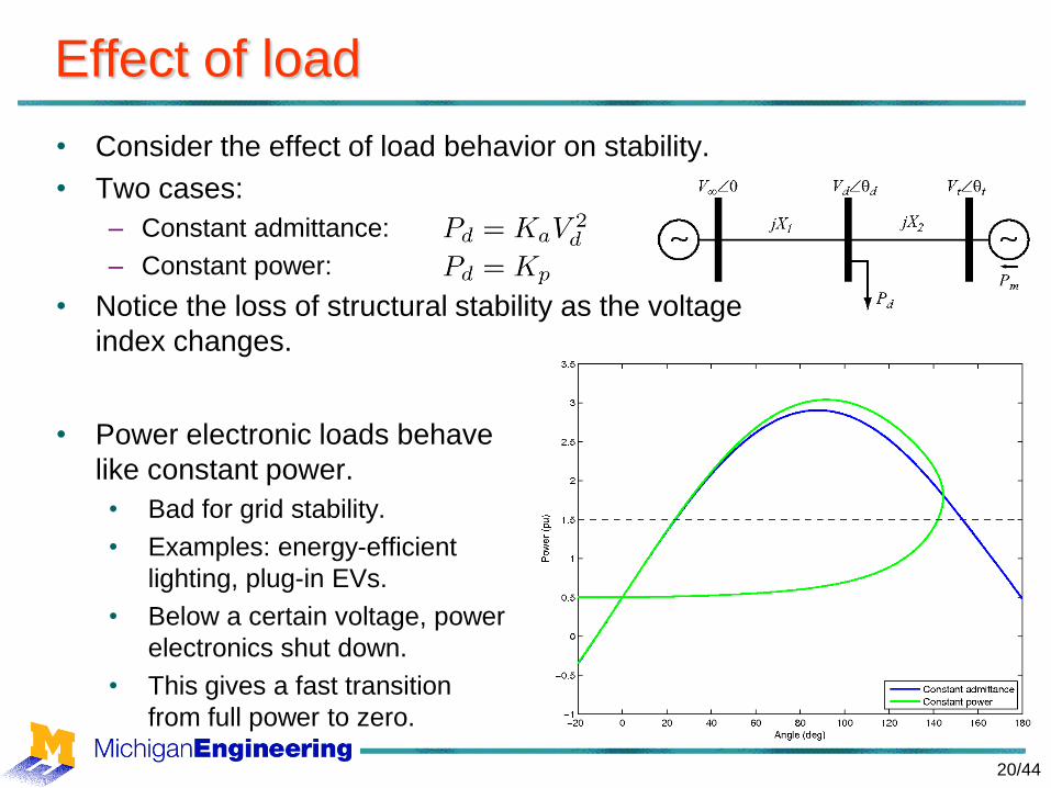
Effect of load

• Consider the effect of load behavior on stability.

• Two cases:

– Constant admittance:

– Constant power:

• Notice the loss of structural stability as the voltage

index changes.

• Power electronic loads behave

like constant power.

• Bad for grid stability.

• Examples: energy-efficient

lighting, plug-in EVs.

• Below a certain voltage, power

electronics shut down.

• This gives a fast transition

from full power to zero.

20/44

Voltage collapse

• Voltage collapse occurs when load-end dynamics

attempt to restore power consumption beyond the

capability of the supply system.

– Power systems have a finite supply capability.

• For this example, two

solutions exist for

viable loads.

• Solutions coalesce at

the load bifurcation

point.

– Known as the point of

maximum loadability.

21/44

Load restoration dynamics (1)

• Transformers are frequently used to regulate load-

bus voltages.

• Sequence of events:

– Line trips out, raising the network impedance.

– Load-bus voltage drops, so transformer increases its tap

ratio to try to restore the voltage.

– Load is voltage dependent, so the voltage increase causes

the load to increase.

– The increasing load draws more current across the network,

causing the voltage to drop further.

22/44

Load restoration dynamics (2)

23/44

Load synchronizing events

• “Fault induced delayed voltage recovery” (FIDVR)

has occurred when a temporary voltage dip causes

large numbers of air-conditioners to stall.

• WECC load model:

24/44

Generator voltage control

• Voltage control is achieved by an “automatic voltage regulator” (AVR) which

adjusts the generator field voltage.

• An increase in the field voltage will result in an increase in the reactive

power produced by the generator, and hence in the terminal voltage.

• If field current becomes excessive, an over-excitation limiter will operate to

reduce the field voltage. The terminal voltage will subsequently fall.

• High-gain voltage control can destabilize angle dynamics.

Typical model for static AVR/PSS

25/44

Generator governor (droop) control

• Active power (primary) regulation is achieved by a governor.

– If frequency is less than desired, increase mechanical torque.

– Decrease mechanical torque if frequency is high.

• For a steam plant, torque is controlled by adjusting the steam value,

for a hydro unit control vanes regulate the flow of water delivered by

the penstock.

• If all generators were to

regulate frequency to a

nominal set-point, hunting

would result.

– This is overcome through the

use of a droop characteristic.

• Primary regulation typically

operates within 10-30 sec.

– Governed by ramp-rate

limits.

26/44

Primary frequency response • Transient frequency response of the Nordic system after loss of

1000 MW generating unit, November 1983.

Time (sec)

Fre

qu

en

cy (

Hz)

Loss of

generation

System inertia governs the

rate of frequency decline

Load damping and governor action

establish the frequency nadir

Droop control drives

frequency restoration

Offset due

to droop

27/44

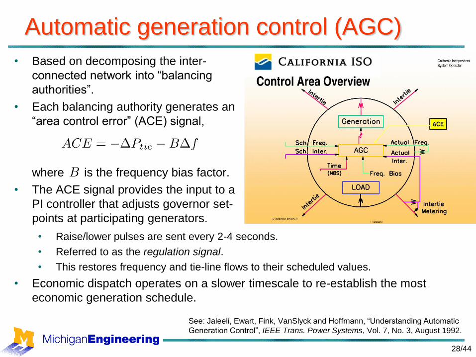
Automatic generation control (AGC)

• Based on decomposing the inter-

connected network into “balancing

authorities”.

• Each balancing authority generates an

“area control error” (ACE) signal,

where is the frequency bias factor.

• The ACE signal provides the input to a

PI controller that adjusts governor set-

points at participating generators.

• Raise/lower pulses are sent every 2-4 seconds.

• Referred to as the regulation signal.

• This restores frequency and tie-line flows to their scheduled values.

• Economic dispatch operates on a slower timescale to re-establish the most

economic generation schedule.

See: Jaleeli, Ewart, Fink, VanSlyck and Hoffmann, “Understanding Automatic

Generation Control”, IEEE Trans. Power Systems, Vol. 7, No. 3, August 1992.

28/44

AGC implementation

29/44

Typical regulation signal

• Example from PJM:

30/44

Operating reserves • Multiple levels of frequency control.

– Primary frequency control is performed by generator governors.

– Secondary frequency control is performed by AGC.

• Spinning reserve is the generating capacity that is on-line, and that is in

excess of the load demand.

– Should be sufficient to cover the loss of the largest generating unit, or loss of the

largest interconnecting tie-line, plus a safety margin.

– The variability of wind power necessitates a higher safety margin.

– Spinning reserve should be distributed over numerous generators.

• Generators have limits on the rate at which they can increase output.

• Reserves also include:

– Interruptible loads.

– Quick-start generation:

gas turbines (simple

cycle), diesel units,

hydro units.

PJM reserve categories

31/44

Corrective control using MPC

Setpoints

of

control

resources

Corrective

actions

Optimal

System

Trajectory

Level 1

Every 6

hours

Forecast

Level 2

Every 15

minutes

Current

Conditions

Level 3

Continuous

Monitoring

Limit

violation

contingency

Model

update

Operational

Status

32/44

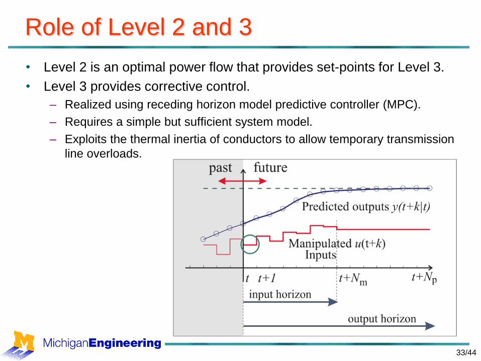
Role of Level 2 and 3

• Level 2 is an optimal power flow that provides set-points for Level 3.

• Level 3 provides corrective control.

– Realized using receding horizon model predictive controller (MPC).

– Requires a simple but sufficient system model.

– Exploits the thermal inertia of conductors to allow temporary transmission

line overloads.

33/44

Level 3 MPC description (1)

• Level 3 employs:

– DC power flow model for active power.

– Piecewise linear relaxation of active line losses.

– Linearized temperature dynamics of transmission lines.

– Standard linear model of energy storage (integrator dynamics).

34/44

Coupling of inputs

and dynamic states

is achieved through

algebraic states

that arise from

power balance

Level 3 MPC description (2)

35

Example

• Standard RTS-96 test case.

Generator Load Throughput Storage/Wind Outage

36/44

Results

• Base-case undergoes cascading failure (5 more lines

trip), and voltage collapse occurs around 29 minutes.

• Level 3 MPC alleviates temperature overloads, so no

further lines trip.

– Employs storage to manage overloads.

– Curtails wind at the appropriate times.

– Brings system to economic set-points.

– Rejects errors due to model approximation.

• Larger horizons less expensive control, higher line

temperatures.

37/44

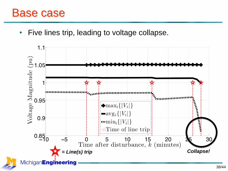
Base case

• Five lines trip, leading to voltage collapse.

Collapse! = Line(s) trip

38/44

MPC response (1)

• Maximum line temperatures.

Level 3 MPC bring temperatures down below limits

Base case - increasing

temperatures.

39/44

MPC response (2)

• Maximum line flows.

Base case – large line

overloads.

Level 3 MPC manages overloads

40/44

MPC response (3)

• Aggregate storage injections.

Respond to outage by

reducing injections.

Returned to optimal set points.

Increase injections to reach SOC set-points.

41/44

MPC response (4)

• Aggregate load curtailment.

All load is restored in the

longer term.

Larger horizon - less load shed.

42/44

MPC response (5)

• MPC objective function value.

43/44

Conclusions

• Power systems are nonlinear, non-smooth,

differential-algebraic systems.

– Hybrid dynamical systems.

• A variety of controls, from local to wide-area, are

used to ensure reliable, robust behaviour.

• Future directions:

– Corrective control reduces reliance on conservative N-1

preventative strategies.

– The variability inherent in renewable generation will

challenge existing control structures.

– There are enormous opportunities for exploiting responsive,

non-disruptive load control.

44/44