highly scalable graph search for the graph500 … scalable graph search for the graph500 benchmark...
TRANSCRIPT
Highly Scalable Graph Search
for the Graph500 Benchmark Koji Ueno
Tokyo Institute of Technology / JST CREST
Toyotaro Suzumura Tokyo Institute of Technology
IBM Research – Tokyo / JST CREST
ABSTRACT
Graph500 is a new benchmark to rank supercomputers with a
large-scale graph search problem. We found that the provided
reference implementations are not scalable in a large distributed
environment. We devised an optimized method based on 2D
partitioning and other methods such as communication
compression and vertex sorting. Our optimized implementation
can handle BFS (Breadth First Search) of a large graph with 236
(68.7 billion vertices) and 240 (1.1 trillion) edges in 10.58 seconds
while using 1366 nodes and 16,392 CPU cores. This performance
corresponds to 103.9 GE/s. We also studied the performance
characteristics of our optimized implementation and reference
implementations on a large distributed memory supercomputer
with a Fat-Tree-based Infiniband network.
Categories and Subject Descriptors
G.2.2 [Discrete Mathematics]: Graph Theory – Graph
algorithms; D.1.3 [Programming Techniques]: Concurrent
Programming – Distributed programming
General Terms
Algorithms, Performance.
Keywords
Graph500, BFS, Supercomputer
1. INTRODUCTION Large-scale graph analysis is a hot topic for various fields of study,
such as social networks, micro-blogs, protein-protein interactions,
and the connectivity of the Web. The numbers of vertices in the
analyzed graph networks have grown from billions to tens of
billions and the edges have grown from tens of billions to
hundreds of billions. Since 1994, the best known de facto ranking
of the world’s fastest computers is TOP500, which is based on a
high performance Linpack benchmark for linear equations. As an
alternative to Linpack, Graph500 [1] was recently developed. We
conducted a thorough study of the algorithms of the reference
implementations and their performance in an earlier paper [19].
Based on that work, we now propose a scalable and high-
performance implementation of an optimized Graph500
benchmark for large distributed environments.
Here are the main contributions of our new work:
1. Optimization of the parallel level-synchronized BFS
(Breadth-First Search) method to improve the cache-hit ratio
through various optimizations in the 2D partitioning, graph
structure and vertex sorting.
2. Optimization of the complete flow of the Graph500 as a
lighter-weight benchmark with better graph construction and
validation.
3. A new traversal record of 103.9 giga-edges/second with our
optimized method on the currently 5th-ranked Tsubame 2.0
supercomputer.
4. A thorough study of the performance characteristics of our
optimized method and those of the reference
implementations.
Here is the organization of our paper. In Section 2, we give an
overview of Graph500 and parallel BFS algorithms. In Section 3,
we describe the scalability problems of the reference
implementations. We explain the proposed optimized BFS
method in Section 4, and the optimized graph construction and
validation in Section 5. In Section 6, we describe our performance
evaluation and give detailed profiles from our optimized method
running on the Tsubame 2.0 supercomputer. We discuss our
findings in Section 7, review related work in Section 8, and
conclude and consider future work in Section 9.
2. GRAPH500 AND PARALLEL BFS
ALGORITHMS In this section, we give an overview of the Graph500 benchmark
[1], the parallel level-synchronized BFS method, and then the
mapping of this method for the sparse-matrix vector
multiplication.
2.1 Graph500 Benchmark In contrast to the computation-intensive benchmark used by
TOP500, Graph500 is a data-intensive benchmark. It does
breadth-first searches in undirected large graphs generated by a
scalable data generator based on a Kronecker graph [16]. The
benchmark has two kernels: Kernel 1 constructs an undirected
graph from the graph generator in a format usable by Kernel 2.
The first kernel transforms the edge tuples (pairs of start and end
vertices) to efficient data structures with sparse formats, such as
CSR (Compressed Sparse Row) or CSC (Compressed Sparse
Column). Then Kernel 2 does a breadth-first search of the graph
from a randomly chosen source vertex in the graph.
The benchmark uses the elapsed times for both kernels, but the
rankings for Graph500 are determined by how large the problem
Permission to make digital or hard copies of all or part of this work for
personal or classroom use is granted without fee provided that copies are
not made or distributed for profit or commercial advantage and that
copies bear this notice and the full citation on the first page. To copy
otherwise, or republish, to post on servers or to redistribute to lists,
requires prior specific permission and/or a fee.
HPDC’12, June 18–22, 2012, Delft, The Netherlands.
Copyright 2012 ACM 978-1-4503-0805-2/12/06...$10.00.
is and by the throughput in TEPS (Traversed Edges Per Second).
This means that the ranking results basically depend on the time
consumed by the second kernel.
After both kernels have finished, there is a validation phase to
check if the result is correct. When the amount of data is
extremely large, it becomes difficult to show that the resulting
breadth-first tree matches the reference result. Therefore the
validation phase uses 5 validation rules. For example, the first rule
is that the BFS graph is a tree and does not contain any cycles.
There are six problem sizes: toy, mini, small, medium, large, and
huge. Each problem solves a different size graph defined by a
Scale parameter, which is the base 2 logarithm of the number of
vertices. For example, the level Scale 26 for toy means 226 and
corresponds to 1010 bytes occupying 17 GB of memory. The six
Scale values are 26, 29, 32, 36, 39, and 42 for the six classes. The
largest problem, huge (Scale 42), needs to handle around 1.1 PB
of memory. As of this writing, Scale 38 is the largest that has been
solved by a top-ranked supercomputer.
2.2 Level-synchronized BFS All of the MPI reference implementation algorithms of the
Graph500 benchmark use a “level-synchronized breadth-first
search”, which means that all of the vertices at a given level of the
BFS tree will be processed (potentially in parallel) before any
vertices from a lower level in the tree are processed. The details of
the level-synchronized BFS are explained in [2][3].
Algorithm I: Level-synchronized BFS
1 for all vertices v parallel do
2 | PRED[v]← -1;
3 | VISITED [v] ← 0;
4 PRED [r] ← 0
5 VISITED[r] ← 1
6 Enqueue(CQ, r)
7 While CQ != Empty do
8 | NQ ← empty
9 | for all u in CQ in parallel do
10 | | u ← Dequeue(CQ)
11 | | for each v adjacent to u in parallel do
12 | | | if VISITED [v] = 0 then
13 | | | | VISITED [v] ← 1;
14 | | | | PRED [v] ← u;
15 | | | | Enqueue(NQ, v)
16 | swap(CQ, NQ);
Algorithm I is the abstract pseudocode for the algorithm that
implements level-synchronized BFS. Each processor has two
queues, CQ and NQ, and two arrays, PRED for a predecessor
array and VISITED to track whether or not each vertex has been
visited.
At any given time, CQ (Current Queue) is the set of vertices that
must be visited at the current level. At level 1, CQ will contain the
neighbors of r, so at level 2, it will contain their pending
neighbors (the neighboring vertices that have not been visited at
levels 0 or 1). The algorithm also maintains NQ (Next Queue),
containing the vertices that should be visited at the next level.
After visiting all of the nodes at each level, the queues CQ and
NQ are swapped at line 16.
VISITED is a bitmap that represents each vertex with one bit.
Each bit of VISITED is 1 if the corresponding vertex has been
already visited and 0 if not. PRED has predecessor vertices for
each vertex. If an unvisited vertex v is found at line 12, the vertex
u is the predecessor vertex of the vertex v at line 14. When we
complete BFS, PRED forms a BFS tree, the output of kernel2 in
the Graph500 benchmark.
The Graph500 benchmark provides 4 different reference
implementations based on this level-synchronized BFS method.
Their details and algorithms appear in an earlier paper [19].
However we found out that the fundamental concept of the level
synchronized BFS can be viewed as a sparse-matrix vector
multiplication. With reference to the detailed algorithmic
explanations in [19], we only explain the basic BFS method here.
2.3 Representing Level-Synchronized BFS as
Sparse-Matrix Vector Multiplication The level-synchronized BFS in II-B is analogous to a Sparse-
Matrix Vector multiplication (SpMV) [20] which is computed as
y = Ax where x and y are vectors and A is a sparse matrix.
A is an adjacency matrix for a graph. Each element of this matrix
is 1 if the corresponding edge exists and 0 if not. The vector x
corresponds to CQ (Current Queue) where x(v) = 1 if the vertex v
is contained in CQ and x(v) = 0 if not. x(v) means the v-th element
of vector x. Then the neighboring vertices of CQ can be
represented as the vertex v where y(v) 1. We get the neighboring
vertices from SpMV. Then we can compute the lines 12 to 15 in
the Algorithm I.
2.4 Mapping Reference Implementations to
SpMV In a distributed memory environment, the graph data and vertex
data must be distributed. There are four MPI-based reference
implementation of Graph500: replicated-csr (R-CSR), replicated-
csc (R-CSC), simple (SIM), and one_sided (ONE-SIDED).
All four of the reference implementations use 1D partitioning
method. The method of vertex distribution is the same in these
four implementations. Assume that we have a total of P
processors. VISITED, PRED and NQ are simply divided into P
blocks and each processor handles one block. There are two
partitioning methods for the sparse matrix shown in Figure 1. For
the Figure 1, we assume that the edge list of the given vertex is a
column of the matrix. With the vertical partitioning (left), each
processor has the edges incident to the vertices the processor
owns. With the horizontal partitioning (right), each processor has
the edges emanating from the vertices the processor owns. Figure
1 also shows how SpMV can be computed in parallel with P
processors. The computation of the reference implementations can
be abstracted as the computation of SpMV. R-CSR and R-CSC
use vertical partitioning for SpMV while SIM and ONE-SIDED
use horizontal partitioning for SpMV.
,
Figure 1. SpMV with vertical and horizontal partitioning.

3. SCALABILITY ISSUES OF REFERENCE
IMPLEMENTATIONS In this section we give overviews of three reference
implementations of Graph500, R-CSR (replicatedc-csr), R-CSC
(replicated-csc), and SIM (simple) and we use experiments and
quantitative data to show why none of these algorithms can scale
well in large systems.
Before moving to the detailed descriptions of each
implementation, we need to cover how CQ (Current Queue) is
implemented in the reference implementations. The reference
implementations also use bitmaps with one bit for each vertex in
CQ and NQ. In these bitmaps, if a certain vertex v is in a queue
(CQ or NQ), then the bit that corresponds to that vertex v is 1 and
if not, then the bit is 0.
We categorize the reference implementations into replication-
based and non-replicated methods, which are described in
Sections 3.1 and 3.2. Then in Section 3.3 we present a scalable
BFS approach with 2D partitioning.
3.1 Replication-based method
3.1.1 Algorithm Description For the R-CSR and R-CSC methods that divide an adjacency
matrix vertically, CQ is duplicated to all of the processes. Then
each processor independently computes NQ for its own portion.
Copying CQ to all of the processors means each processor sends
its own portion of NQ to all of the other processors. CQ (and NQ)
is represented as a relatively small bitmap. For relatively small
problems with limited amounts of distribution, the amounts of
communication data are reasonable and this method is effective.
However, since the size of CQ is proportional to the number of
vertices in the entire graph, this copying operation leads to a large
amount of communication for large problems with large
distribution.
3.1.2 Quantitative Evaluation for Scalability Figure 2 shows the communication data volume for each node
with the replication-based implementation and SCALE of 26 for
each node as the problem size. This is a weak-scaling version, and
computes the theoretical results when using 2 MPI processes per
node. In such a weak-scaling setting, the number of vertices
increases in proportion to the increasing number of nodes. This
result clearly shows that the Replication-based method is not
scalable for a large distributed environment.
0
20
40
60
80
100
120
140
Me
ssag
e S
ize
pe
r N
od
e(G
B)
# of nodes
replicated (reference)
Figure 2. Theoretical message size per node (GB)
3.2 Non-replicated Method
3.2.1 Algorithm Description The simple reference implementation or SIM that divides an
adjacent matrix in a horizontal fashion, locates the portion of the
CQ by dividing it into P . The NQ queue is already divided into
P blocks, and so each processor can use the NQ queue from the
previous level as the CQ of the current level.
Edge lists of the vertices in CQ are merged to form a set N of
edges. The edges of a set N are the edges emanating from the
vertices in CQ and incident to the neighboring vertices. These N
include both the edges to be handled by the local processor and by
other processors. The edges incident to the vertex owned by
remote processors are transmitted to those processors.
The number of edges to be transmitted to remote processors can
be up to the number of edges of the adjacency matrix owned by
the sender-side processor. Thus the communication data volume is
constant without regard to the number of nodes.
However, the Replication-based method with vertical partitioning
transmits CQ as a bitmap. On the other hand in the simple
implementation, SIM needs to send edges, pairs of a CQ vertex
and neighboring vertex because the predecessor vertex is needed
to update PRED, the predecessor array. Therefore, the
Replication-based approach with vertical partitioning is better
than the simple approach in a small-scale environment with fewer
nodes.
3.2.2 Quantitative Evaluation for Scalability The other two reference implementations with horizontal
partitioning are called “simple” and “one_sided”. In these
implementations all-to-all communication that sends a different
data set to each of the other processors is needed when sending
the set of N edges. This all-to-all communication is not scalable
for large distributed environments.
Figure 3 shows the communication speed of the all-to-all
communication on Tsubame 2.0 when using 4 MPI processes per
node. We used MVAPICH2 1.6 as the MPI implementation. The
communication was implemented with the MPI_Alltoall function,
and we used three different transmission buffer sizes, 64 MB, 256
MB, and 1,024 MB.
The amount of data that each node transmits to other nodes is 4
MB when using the 1,024 MB buffer size, 64 nodes, and 256 MPI
processes. The results shown in Figure 3 show that the all-to-all
communication is not scalable.
0
500
1000
1500
2000
2500
3000
32 64 128 256 512
Ave
rage
Dat
arat
e p
er
No
de
(M
B/s
)
# of nodes
64MB Buffer
256MB Buffer
1024MB Buffer
Figure 3. Average data rate per node with all-to-all
communication

With 512 nodes, the performance is quite slow even with a small
buffer size such as 64 MB. Also, even if we use 1,024 MB as the
buffer size, the performance is 1/4 of 32 nodes.
Our experimental testbed, Tsubame 2.0, uses a Fat-Tree structure
with its Infiniband network. If the theoretical peak performance
were achieved, there would be no performance degradation even
for all-to-all communication is among all of the nodes. However,
the communication latency cannot be ignored in a large system.
The actual performance is always less than the theoretical
maximum.
3.3 Scalable Approach: 2D Partitioning-
Based BFS To solve the scalability problems described in Section 3.1 and
Section 3.2, a scalable distributed parallel breadth-first search
algorithm was proposed in [4]. Their scalable approach uses a
level-synchronized BFS and 2D partitioning technique to reduces
the communication costs since it can handle both vertical and
horizontal partitioning, unlike 1D partitioning. Our proposed
method optimizes this 2D partitioning technique and also uses
some other optimization techniques. Here is a brief overview of
the 2D partitioning technique.
Assume that we have a total of P processors, where the
CRP processors are logically deployed in a two dimensional
mesh which has R rows and C columns. We use the terms
processor-row and processor-column with respect to this
processor mesh. Adjacency matrix is divided as shown in Figure 4
and the processor ),( ji is responsible for handling the C blocks
from )1(
, jiA to
)(
,
C
jiA . The vertices are divided into CR blocks
and the processor ),( ji handles the k-th block, where k is
computed as iRj )1( .
Figure 4. 2D Partitioning Based BFS [4]
Each level of the level-synchronized BFS method with 2D
partitioning is done in 2 communication phases called “expand”
and “fold”. In the expand phase, every processor copies its CQ to
all of the other processors in the same processor-column, similar
to vertical 1D partitioning. Then the edge lists of the vertices in
CQ are merged to form a set N. In the fold phase, each processor
sends the edges of N to the owner of their incident vertices,
similar to horizontal 1D partitioning. With the 2D partitioning,
these owners are in the same processor-row. 2D partitioning
method is equivalent to a method of combining the two types of
1D partitioning. If C is 1, this corresponds to the vertical 1D
partitioning and if R is 1, it corresponds to the horizontal 1D
partitioning.
The advantage of 2D partitioning is to reduce the number of
processors that need to communicate. Both types of 1D
partitioning require all-to-all communication. However, with the
2D partitioning, each processor only communicates with the
processors in the processor-row and the processor-column.
4. U-BFS: SCALABLE BFS METHOD Our BFS implementation is based on a 2D partitioning method
and is highly optimized for a large-scale distributed computing
environment by using various optimization techniques. In this
section we present these techniques. As described in Section 3.3,
in the 2D partitioning, the CRP processors are deployed in
a CR mesh.
4.1 Overview of Oprimized 2D Partioning-
based BFS (U-BFS) Our U-BFS optimization also uses the 2D partitioning technique.
The communication method of the expand phase is the same
approach as R-CSC, one of the reference implementations. Each
set of vertices in CQ is represented as a bitmap and each processor
gathers CQ at each level by using the MPI_AllGather function.
The communication of the fold phase is optimized in our
implementation by compression of the data described in Section
4.2. Because the amount of data communicated in each fold phase
is much larger than that of the expand phase when we use a naïve
method, compression of the data is important.
We divide the processing of the fold phase into senders and
receivers. The senders send the edges emanating from the vertices
in CQ as compressed data. The receivers receive data from the
senders, decompress the data to edges, and process edges. Both
senders and receivers are handled by multiple parallel threads and
the communication can be done asynchronously. Our proposed
method has highly efficient processing with this parallel and
asynchronous communication.
In addition, our method can efficiently utilize the CPU caches by
vertex sorting (Section 4.4), binding the threads to CPU cores
(Section 4.3), and then giving higher priority to the receiver
threads (Section 4.3) to reduce the cache replacements from
thread switching.
The algorithm appears as Algorithm II. CQ and NQ are bitmaps.
In Lines 1-2, NQ is initialized and the BFS root is inserted into
NQ in line 3. Lines 5-10 are done by all of the processors. Line 6
is the expand communication. In Line 7, Task A and Task B run
in parallel. Task A is the receiver processing and Task B is the
sender processing.

Algorithm II: Optimized 2D partitioning algorithm
Variables: MAP which is described in the Section 4.4 is for
conversion from the sorted number to the original number.
Main
1 for all vertexes lu in NQ do
2 | NQ[lu] ← 0
3 NQ [root] ← 1
4 fork;
5 for level = 1 to
6 | CQ ← all gather NQ in this processor-column;
7 | parallel Task A and Task B
8 | Synchronize;
9 | if NQ = for all processors then
10 | | terminate loop;
11 join;
Task A (sender)
1 for all vertexes u in CQ parallel do (contiguous access)
2 | if CQ [u] = 1 then
3 | for each vertex v’ adjacent to u do
4 | | compress the edge (u, v’) and send it to the owner of vertex v’
Task B (receiver)
1 for each received data parallel do
2 | decompress the data and get the edge (u, v’)
3 | if visited[v’] = 0 then
4 | | VISITED[v’] ← 1;
5 | | v ← MAP[v’];
6 | | PRED[v] ←u;
7 | | NQ [v] ← 1;
4.2 Optimized Communication with Data
Compression The compression of communication data is greatly important
because the bottleneck of the distributed BFS is often the
communication. We optimized the communication of the fold
phase because the amount of data communicated in the fold phase
is much larger than that of the expand phase when we use a naïve
method. In the fold phase, sender side sends the edges emanating
from the vertices in CQ. The edges are represented as a list of a
tuple (u, v) where u is the vertex of CQ and v is the neighboring
vertex of CQ. We compress vertex u and v with different
compression techniques.
Here is our compression method for vertex u. Since CQ is a
bitmap, by checking CQ in order of bitmap array, the vertices in u
will be sorted in ascending-order. Thus the average difference
between two vertex u in successive edges will be small. The
vertex u is represented by simply encoding the difference from the
prior tuple with variable-length quantity which is used by the
standard MIDI file format and Google’s protocol buffers etc. We
use general variable-length quantity (VLQ) for unsigned integer.
An integer value will be one or more bytes. Smaller numbers will
be smaller number of bytes. The most significant bit (MSB) of
each byte indicates whether another VLQ byte follows. If the
MSB is 1, another VLQ byte follows and if 0, this is the last byte
of the integer. The rest 7 bits of each byte form an integer. The
least significant will be first in a stream.
For example, we assume that the CQ bitmap is ‘01100001’ which
means three vertices 1, 2 and 7 are in the CQ and we also assume
that the numbers of edges emanating from the vertices 1, 2 and 7
are 2, 1 and 3 respectively. The series of vertices u will be '1, 1, 2,
7, 7, 7’ because we check the CQ in order. Then we will get the
difference from the prior vertex, ‘-, 0, 1, 5, 0, 0’. With VLQ, a
smaller number will be encoded into smaller number of bytes.
Therefore, we can compress the vertices u.
For the compression of vertex v, each edge (u, v) will be sent to
the owner of vertex v. We distribute these vertices with a round
robin method. The owner of vertex v’ is computed by dividing v
by P . For example, the owner of vertex v )(proclocal
vPv is
procv . Thus by sending Pvv /
local instead of v, we can reduce
the size of the data for vertex v.
The data representation of vertex u is compressed by using the
differences from the preceding data. However to support multi-
threaded processing, we need to introduce a packet, a unit which
can be decoded independently. If we send a series of edges in one
packet containing (300, 533), (301, 12), (301, 63), (303, 1222) as
(u, v), then the data representation of the vertex u without VLQ
encoding, but with the difference technique is “300, 1, 0, 2”. With
the VLQ encoding, it becomes “0xAC, 0x01, 0x01, 0x00, 0x02”.
When there are P processors, the data representation of the vertex
v is “8, 0, 0, 19”. Without this optimization, the size of each data
tuple (v, u) would be 16 bytes, since each vertex is represented as
8 bytes, but with this optimization, the data size is about 5 bytes
on average, since the vertex v consumes 4 bytes and the vertex u
consumes about 1 byte as long as the difference between the
contiguous values is less than 128 with the VLQ encoding.
4.3 Parallelizing the Sender and Receiver
Processing Our optimized implementation uses hybrid parallelism of MPI
and OpenMP for communication and computational efficiency.
As our multi-threading strategy to use N CPU cores for MPI
processes, we run (N-1) threads for the sender-side processing
(Task A) and (N-1) threads for the receiver side (Task B), and
only 1 thread for communication. In total, (2N-1) threads run in
parallel. The communication dataflow in the fold phase appears in
Communication thread Task BTask A
Each thread has
own packet buffers
packet
Send buffer Receive burffer
1KB~4KB
2MB~8MB
Using
asynchronous IO
Decode edges and
update VIDITED
and NQ
Extract edges
emanating from the
vertices in CQ
Packet index
Communication thread
creates packet indices for
multi-threaded processing
Figure 5. A dataflow diagram of the fold communication.
Figure 5. Each thread at the sender side reads the graph data and
CQ, compress edges and then store compressed edge data into the
packet buffer prepared for each sender thread.
Once the packet buffer is full, the data is passed to the
communication thread and emitted with the asynchronous MPI
sender function MPI_Isend. When a communication thread
receives the data, it creates a packet index for multi-threaded
processing and passes it to the receiver thread. Once the receiver
thread receives the packet index and the data, the thread decodes
it, updates the VISITED bitmap, and creates NQ.
The receiver thread decodes the incoming edge (v, u) where u is
the vertex of CQ and v is the neighboring vertex of CQ,
determines whether vertex v was already visited by checking the
VISITED bitmap, and if not, updates the VISITED bitmap and
NQ. However since the incoming vertices v are received at
random, the random access to the VISITED bitmap can degrade
the performance. We optimize updating VISITED bitmap in the
next section.
We also optimize for the NUMA architecture. If we have N CPU
cores for MPI processes, then (2N – 1) threads are created. Unless
these threads are bound to a CPU, the OS scheduler will allocate
more than N CPU cores. For a multi-socket CPU like that of
Tsubame 2.0, if a thread is moved to another CPU core at a
different CPU socket, then the cache hit ratio is reduced. Also, for
a NUMA architecture, the memory and the CPU where the data
processing thread is running should be kept close together.
To reduce cache misses due to thread switches, the threads for the
receiver side have higher priority to the threads for the sender side.
This thread priority also reduces the amount of buffers required
for receiver processing.
4.4 Improving Cache Hit Ratio with Vertex
Sorting We explained in the previous section that each receiver thread
(Task B) generates random memory access to the VISITED
bitmap, which lowers the cache hit ratio. The distribution of the
degrees follows Zipf's law as observed in our earlier work [19],
since Graph500 uses a Kronecker graph [16]. The frequency of
access to VISITED is determined by the vertex degree (the
number of edges of each vertex). If the degree of vertex v is high,
then v-th element of VISITED will be accessed more frequently.
The high cost of random memory access can be reduced by
sorting the vertices in decreasing order of degrees. We call this
optimization Vertex Sorting.
To optimize accessing the VISITED bitmap, we use the sorted
order in the row index of the adjacent matrix. We do not use the
sorted order in the column index. If we use the sorted order in
both row and column index, the conversion of PRED from the
sorted order to original order is necessary. This conversion needs
all-to-all collective communication which we need to pay
expensive cost. Therefore, in the adjacent matrix, the row index
and the column index for the same vertex are different.
In Algorithm II, v’ is the sorted number and v is the original
number. The number we get from the adjacent matrix is the sorted
one. We change the sorted number to the original one in line 5 of
Task B (receiver-side processing) by using MAP.
In the 2D partitioning, vertices are divided into CR blocks and
each block is allocated to a processor. We sort the vertices only in
a local block. Therefore, Vertex Sorting does not affect the vertex
partitioning and the graph partitioning. The adjacent matrix and
the MAP in Algorithm II are created in the construction phase
(kernel 1). The method of sorting the vertices in the construction
phase is described in Section 5.1.
5. GRAPH CONSTRUCTION FOR U-BFS
AND OPTIMIZING VALIDATION In this section we present the method of the construction phase for
optimized BFS described in the previous section and the method
of optimizing validation.
The current Graph500 benchmark must conduct 64 iterations of
the BFS executions and validations. The validation phase
dominates the overall time of the Graph500 benchmark, and so it
is critically important to accelerate this phase to speed up the
entire experiment.
5.1 Graph Construction In the construction phase, we construct a sparse matrix
representation of the graph from the edge list generated in the
generation phase. Our optimized algorithm of the construction
phase is shown in Algorithm III.
Algorithm III: Graph Construction Input: L is a generated edge list.
Output: Two arrays of a sparse matrix representation for the
graph, P and V. P is a pointer array and V is an index array.
MAP for conversion from the sorted number to the original
number.
C and I are arrays that have the same length of P. S is an array
whose length is the number of local vertices.
1 for each column v of local adjacency matrix
2 | P[v] ← 0
3 | C[v] ← 0
4 | I[v] ← 0
5 for each local vertex v
6 | S[v] ← 0
7 for each edge (v0, v1) in L
8 | send edge (v0, v1) to its owner
9 | send edge (v1, v0) to its owner
10 for each received edge (u, v)
11 | C[v] ← C[v] + 1
12 | send vertex v to its owner
13 for each received vertex v
14 | S[v] ← S[v] + 1
15 sort S and create MAP for conversion from sorted
number to original number and MAP' for inverse
conversion
16 for v is 1 to the number of columns of local adjacency
matrix
17 | P[v] ← P[v-1] + C[v]
18 for each edge (v0, v1) in L
19 | send edge (v0, v1) to its owner
20 | send edge (v1, v0) to its owner
21 for each received edge (u, v)
22 | send vertex u to its owner
23 | receive vertex u and send MAP'[u] to sender processor
24 | receive MAP'[u] as u'
25 | V[P[v] + I[v]] ← u'
26 | I[v] ← I[v] + 1
In our implementation, the matrix is 2D partitioned. Both edges
and vertices have their owner processor. In Algorithm III, local
adjacency matrix is a portion of the adjacency matrix allocated to
the processor and local vertices are the vertices the processor
owns.
5.2 Validation The validation determines the correctness of the BFS result based
on the edge tuples generated in the graph generation phase. By
profiling the validation phase of the reference implementation, we
found two validation rules in the Graph500 specification
dominating the all-to-all communications.
1) Each edge in the input list has vertices with levels that differ by
at most one or neither is in the BFS tree
2) Each node and its parent are joined by an edge in the original
graph.
A processor that owns an edge tuple (v0, v1) needs to
communicate with the owner processor of v0 and the owner
processor of v1. Implemented in a naïve fashion, this requires all-
to-all communication involving all of the processors, which is not
scalable. We devised an approach that divides the edge tuples
with 2D partitioning and allocates them to each processor before
the first BFS execution. The number of processors involved in
communication is fewer than the original version, making the
work scalable.
6. PERFORMANCE EVALUATION We used Tsubame 2.0, the fifth fastest supercomputer in the
TOP500 list of June 2011, to evaluate the scalability of our
optimized implementation.
6.1 Overview of the Tsubame 2.0
supercomputer Tsubame 2.0 is a production supercomputer operated by the
Global Scientific Information and Computing Center (GSIC) at
the Tokyo Institute of Technology. Tsubame 2.0 has more than
1,400 compute nodes interconnected by high-bandwidth full-
bisection-wide Infiniband fat nodes.
Each Tsubame 2.0 node has two Intel Westmere EP 2.93 GHz
processors (Xeon X5670, 256-KB L2 cache, 12-MB L3), three
NVIDIA Fermi M2050 GPUs, and 50 GB of local memory. The
operating system is SUSE Linux Enterprise 11. Each node has a
theoretical peak of 1.7 teraflops (TFLOPS). The main system
consists of 1,408 computing nodes, and the total peak
performance can reach 2.4 PFLOPS. Each of the CPUs in
Tsubame 2.0 has six physical cores and supports up to 12
hardware threads with Intel’s hyper-threading technology, thus
achieving up to 76 gigaflops (GFLOPS).
The interconnect that links the 1,400 computing nodes with
storage is the latest QDR Infiniband (IB) network, which has 40
Gbps of bandwidth per link. Each computing node is connected to
two IB links, so the communication bandwidth for the node is
about 80 times larger than a fast LAN (1 Gbps). Not only the link
speed at the endpoint nodes, but the network topology of the
entire system heavily affects the performance for large
computations. Tsubame 2.0 uses a full-bisection fat-tree topology,
which handles applications that need more bandwidth than
provided by such topologies as a torus or mesh.
6.2 Evaluation Method In the software environment we used gcc 4.3.4 (OpenMP 2.5) and
MVAPICH2 version 1.6 with a maximum 512 nodes. Tsubame
2.0 is also characterized as a supercomputer with heterogeneous
processors and a large number of GPUs, but we did not use those
parts of the system. Each node of Tsubame 2.0 has 12 physical
CPU cores and 24 virtual cores with SMT (Simultaneous
Multithreading). Our implementation treats 24 cores as a single
node and the same number of processors is allocated to each MPI
process.
In our experiments, the 2D-partitioning-based processor
allocation CR was per Table 1. R and C were determined with
the policy of allocating division numbers as similarly as possible.
The number of MPI processes should be a power of two and the
value of R and C was determined by the MPI processes
irrespective of the number of nodes.
The result in this paper is the maximum performance of 16
iteration BFS runs. But the result of the Graph500 list is the
median of 64 BFS runs. Therefore, there is a little difference
between the performance result in this paper and our official score
of the Graph500 list.
Table 1. The values of R and C with the # of MPI processes
# of MPI processes 1 2 4 8 16 32
R 1 1 2 2 4 4
C 1 2 2 4 4 8
# of MPI processes 64 128 256 512 1024 2048
R 8 8 16 16 32 32
C 8 16 16 32 32 64
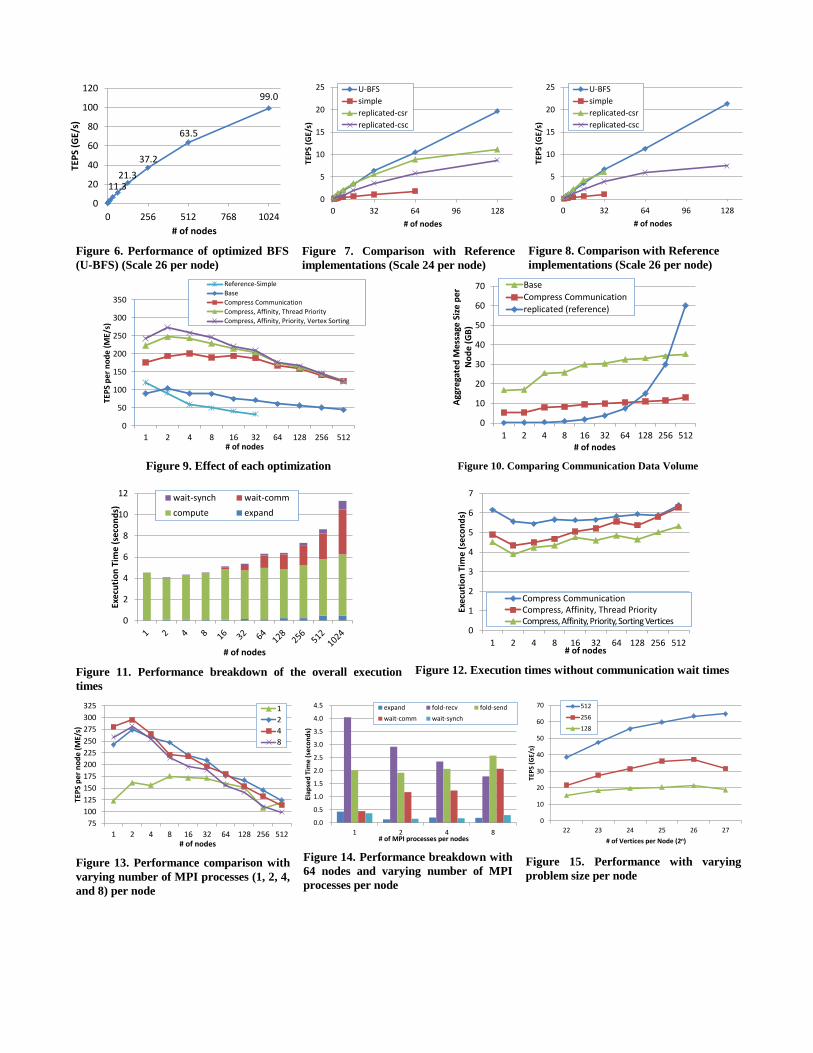
6.3 Performance of U-BFS Figure 6 shows the performance of U-BFS in a weak-scaling
fashion with SCALE 26 per node. We use 2 MPI processes for
each node. We get the performance of 99.0 GE/s (TEPS) with
1024 nodes and SCALE 36. We also conducted the experiment
with 1366 nodes and our optimized implementation achieved
103.9 GE/s (TEPS) with 1366 nodes (16,392 CPU cores) and
SCALE 36.
6.4 Comparison with Reference
Implementations We compared U-BFS with the latest version (2.1.4) of the
reference implementations in Figure 7 and Figure 8. This
experiment was done in a weak-scaling fashion, so the problem
size for each node was held constant, SCALE 24 in Figure 7 and
SCALE 26 in Figure 8. The horizontal axis is the number of
nodes and the vertical axis is the performance in GE/s.
U-BFS and the two reference implementations, R-CSR and R-
CSC use 2 MPI processes for each node. The reference
implementation, simple, uses 16 MPI processes for each node,
since the implementation does not use multithreading parallelism.
As shown in the graph, there were some results that could not be
measured due to problems in the reference implementations.
When the number of nodes is increased for SIM, the system ran
out of memory. With R-CSR and SCALE 32, a validation error
occurred and there was a segmentation fault at higher SCALE
values. With R-CSC, the construction phase crashes above
SCALE 34. Figure 7 and Figure 8 show that U-BFS outperformed
R-CSC and SIM for all of the nodes. With numbers of nodes
fewer than 32, the R-CSR implementation is best, but our method
shows performance advantages with more than 32 nodes. For
example, our optimized method is 2.8 times faster than R-CSR
with 128 nodes and SCALE 26 for each node. (All of the final
problem sizes were SCALE 33.)
11.3 21.3
37.2
63.5
99.0
0
20
40
60
80
100
120
0 256 512 768 1024
TEP
S (G
E/s)
# of nodes
Figure 6. Performance of optimized BFS
(U-BFS) (Scale 26 per node)
0
5
10
15
20
25
0 32 64 96 128
TEP
S (G
E/s)
# of nodes
U-BFS
simple
replicated-csr
replicated-csc
Figure 7. Comparison with Reference
implementations (Scale 24 per node)
0
5
10
15
20
25
0 32 64 96 128
TEP
S (G
E/s)
# of nodes
U-BFS
simple
replicated-csr
replicated-csc
Figure 8. Comparison with Reference
implementations (Scale 26 per node)
0
50
100
150
200
250
300
350
1 2 4 8 16 32 64 128 256 512
TEP
S p
er n
od
e (M
E/s)
# of nodes
Reference-Simple
Base
Compress Communication
Compress, Affinity, Thread Priority
Compress, Affinity, Priority, Vertex Sorting
Figure 9. Effect of each optimization
0
10
20
30
40
50
60
70
1 2 4 8 16 32 64 128 256 512
Agg
rega
ted
Me
ssag
e S
ize
pe
r N
od
e (
GB
)
# of nodes
Base
Compress Communication
replicated (reference)
Figure 10. Comparing Communication Data Volume
0
2
4
6
8
10
12
Exec
uti
on
Tim
e (s
eco
nd
s)
# of nodes
wait-synch wait-comm
compute expand
Figure 11. Performance breakdown of the overall execution
times
0
1
2
3
4
5
6
7
1 2 4 8 16 32 64 128 256 512
Exe
cuti
on
Tim
e (
seco
nd
s)
# of nodes
Compress CommunicationCompress, Affinity, Thread PriorityCompress, Affinity, Priority, Sorting Vertices
Figure 12. Execution times without communication wait times
75
100
125
150
175
200
225
250
275
300
325
1 2 4 8 16 32 64 128 256 512
TEP
S p
er n
od
e (M
E/s)
# of nodes
1
2
4
8
Figure 13. Performance comparison with
varying number of MPI processes (1, 2, 4,
and 8) per node
0.0
0.5
1.0
1.5
2.0
2.5
3.0
3.5
4.0
4.5
1 2 4 8
Elap
sed
Tim
e (
seco
nd
s)
# of MPI processes per nodes
expand fold-recv fold-send
wait-comm wait-synch
Figure 14. Performance breakdown with
64 nodes and varying number of MPI
processes per node
0
10
20
30
40
50
60
70
22 23 24 25 26 27
TEP
S (G
E/s)
# of Vertices per Node (2n)
512
256
128
Figure 15. Performance with varying
problem size per node

6.5 Effect of Each Optimization Figure 9 shows the performance effects of each of our proposed
optimization techniques. For the reference data, we also show the
performance of SIM. The Fold phase, which is the main
computation part of 2D partitioning-based algorithm, uses the
same approach as the simple reference implementation. Therefore,
our optimization should show similar performance characteristics.
We also prepared a “base” version as a multi-threaded
implementation with 2D partitioning. This version parallelizes the
senders and receivers, and also uses asynchronous communication.
Even without any optimizations, this almost doubles the
performance over the simple reference implementation.
Compared with the base version, the communication compression
technique (Section 4.2) boosts the performance by 2 to 3 times.
We also had a maximum of a 27% performance improvement due
to the CPU affinity and the technique (Section 4.3) of giving
higher priority to the receiver processing. Another 10% came
from the technique of vertex sorting (Section 4.4). However, these
optimizations except for the communication compression were
not effective with larger numbers of nodes because the network
communications became the major bottleneck.
Figure 10 compares the communication data volume of our
optimized method and the reference implementation in a weak-
scaling setting. The vertical axis is the transmitted data volume
(GB) per node involved in one traversal of BFS with the SCALE
26 problem size. This profiling used 2 MPI processes per node.
The data volume of the Replication-based reference
implementations including R-CSC and R-CSR is a theoretical
value since we could not measure the data with more than 256
nodes because of the limitations of the reference implementations.
This graph shows the measured data for the 2D-partitioning-based
optimization methods comparing communication compression
and no compression.
The communication data volume increases in proportion to the
number of nodes for the weak-scaling setting since the
Replication-based implementation needs to send CQ to all of the
other processes. Meanwhile, the 2D-based partitioning method is
scalable since the communication data volume becomes relatively
smaller. With the data compression technique used by U-BFS, the
communication data volume can be reduced to around one third of
the base version. For example, the data volume was reduced from
32.3 GB to 13.1 GB with 512 nodes.
Figure 11 shows the breakdown of the execution time with U-BFS
in a weak-scaling setting. The vertical axis is the execution time of
BFS with SCALE 26 for a single node that runs 2 MPI processes.
Since the communication at the fold phase is asynchronous, the
communication waits only occur when the communication cannot
keep up with the computation. The synchronization wait is the
waiting time when synchronizing with all of the other nodes just
before the level-synchronized BFS moves to the next step.
In our profiling results, the communication costs for the Expand
phase is relatively small. A large part of the execution time is
spent in the computations. However with more than 16 nodes, the
communication wait time is increasing, which increases the
overall execution time. This means the bottleneck of U-BFS with
more than 16 nodes is the communication. More analysis appears
in the Discussion section.
With the profiling result, the overall execution time, which
excludes the communication wait time of each optimization, is
shown in Figure 12. This result shows that the execution time
without the communication wait time decreases as expected with
our optimization techniques. This is also observed even with
relatively large numbers of nodes where communications becomes
the bottleneck.
6.6 Performance comparison with varying
number of MPI processes Figure 13 shows the performance characteristics when varying the
number of MPI processes per node in a weak-scaling setting. The
result does not show great differences between 2 or 4 MPI
processes, but the performance is degraded with 1 and 8 MPI
processes.
Figure 14 shows that the processing time at the receiver side
decreases with larger numbers of nodes. The processing time at
the receiver side (which requires the random access to the visited
bitmap) can be reduced by increasing the cache hit ratio, since the
number of vertices allocated for each MPI process decreases with
more MPI processes.
Meanwhile the processing time at the sender side is increasing
with larger numbers of MPI processes. This is because the number
of CPU cores allocated for each MPI process, N, is decreased
since (N-1) threads are running as senders. The communication
time is also increased for 1 and 8 MPI processes. For these
reasons, performance degradation is seen with 1 and 8 MPI
processes per node.
6.7 Performance with varying problem size
per node Figure 15 shows the performance characteristics as the problem
size changes. U-BFS executes 2 MPI processes per node. The
maximum problem size U-BFS can compute on the Tsubame 2.0
environment is SCALE 27. The experimental results shown in
Figure 15 show the best performance is obtained with SCALE 26
per node when using 128 and 256 nodes. With 512 nodes, the
SCALE 27 problem size shows the best performance. Also, we
ran the same experiments with less than 64 nodes for reference,
although our proposed optimization targets large environments.
SCALE 26 per node shows the best performance with 1, 2, 4, 8,
16, 32, and 64 nodes.
6.8 Profiling Execution Time and
Communication Data Size at Each Level Figure 16 compares the reference implementations, R-CSR and R-
CSC, with U-BFS in terms of the execution time at each level of
the level-synchronized BFS method. Note that the reference
implementations only use 32 nodes and our optimized method
uses 128 nodes, but the problem size per node is the same, so this
is a fair comparison.
The Kronecker graph adopted by the Graph500 benchmark is a
scale-free graph. With such a graph, the search range becomes
greatly expanded once it reaches vertexes with high degrees that
have large numbers of edges. Since R-CSR computes the CSR-
based algorithm, the execution time at each level depends on the
number of unvisited vertices.
Therefore this method consumes more time in the shallow
portions. In contrast, R-CSC and U-BFS use the CSC-based
method. Unlike the CSR-based method, the execution time at each
level is almost proportional to the number of adjacent vertices of
CQ.
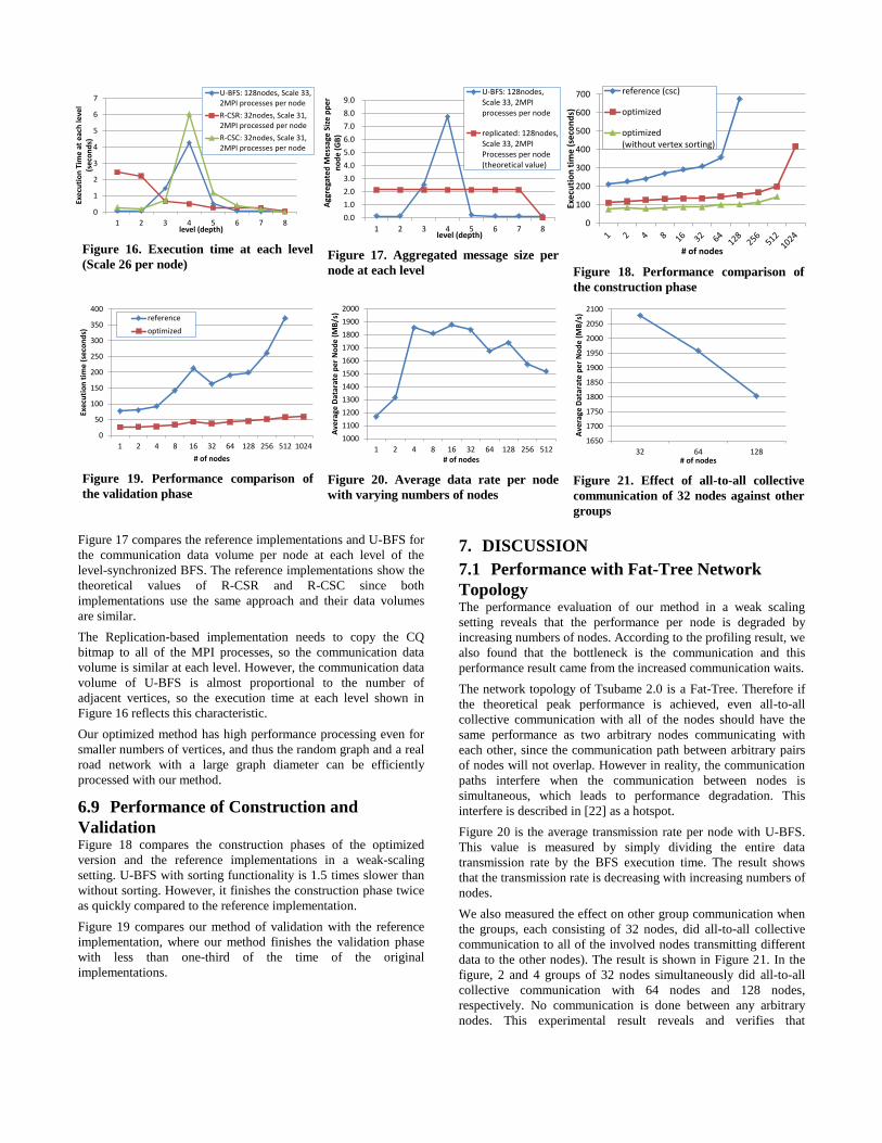
Figure 17 compares the reference implementations and U-BFS for
the communication data volume per node at each level of the
level-synchronized BFS. The reference implementations show the
theoretical values of R-CSR and R-CSC since both
implementations use the same approach and their data volumes
are similar.
The Replication-based implementation needs to copy the CQ
bitmap to all of the MPI processes, so the communication data
volume is similar at each level. However, the communication data
volume of U-BFS is almost proportional to the number of
adjacent vertices, so the execution time at each level shown in
Figure 16 reflects this characteristic.
Our optimized method has high performance processing even for
smaller numbers of vertices, and thus the random graph and a real
road network with a large graph diameter can be efficiently
processed with our method.
6.9 Performance of Construction and
Validation Figure 18 compares the construction phases of the optimized
version and the reference implementations in a weak-scaling
setting. U-BFS with sorting functionality is 1.5 times slower than
without sorting. However, it finishes the construction phase twice
as quickly compared to the reference implementation.
Figure 19 compares our method of validation with the reference
implementation, where our method finishes the validation phase
with less than one-third of the time of the original
implementations.
7. DISCUSSION
7.1 Performance with Fat-Tree Network
Topology The performance evaluation of our method in a weak scaling
setting reveals that the performance per node is degraded by
increasing numbers of nodes. According to the profiling result, we
also found that the bottleneck is the communication and this
performance result came from the increased communication waits.
The network topology of Tsubame 2.0 is a Fat-Tree. Therefore if
the theoretical peak performance is achieved, even all-to-all
collective communication with all of the nodes should have the
same performance as two arbitrary nodes communicating with
each other, since the communication path between arbitrary pairs
of nodes will not overlap. However in reality, the communication
paths interfere when the communication between nodes is
simultaneous, which leads to performance degradation. This
interfere is described in [22] as a hotspot.
Figure 20 is the average transmission rate per node with U-BFS.
This value is measured by simply dividing the entire data
transmission rate by the BFS execution time. The result shows
that the transmission rate is decreasing with increasing numbers of
nodes.
We also measured the effect on other group communication when
the groups, each consisting of 32 nodes, did all-to-all collective
communication to all of the involved nodes transmitting different
data to the other nodes). The result is shown in Figure 21. In the
figure, 2 and 4 groups of 32 nodes simultaneously did all-to-all
collective communication with 64 nodes and 128 nodes,
respectively. No communication is done between any arbitrary
nodes. This experimental result reveals and verifies that
0
1
2
3
4
5
6
7
1 2 3 4 5 6 7 8
Exec
uti
on
Tim
e at
eac
h le
vel
(sec
on
ds)
level (depth)
U-BFS: 128nodes, Scale 33,2MPI processes per node
R-CSR: 32nodes, Scale 31,2MPI processed per node
R-CSC: 32nodes, Scale 31,2MPI processes per node
Figure 16. Execution time at each level
(Scale 26 per node)
0.0
1.0
2.0
3.0
4.0
5.0
6.0
7.0
8.0
9.0
1 2 3 4 5 6 7 8
Agg
rega
ted
Mes
sage
Siz
e p
pe
r n
od
e (
GB
)
level (depth)
U-BFS: 128nodes,Scale 33, 2MPIprocesses per node
replicated: 128nodes,Scale 33, 2MPIProcesses per node(theoretical value)
Figure 17. Aggregated message size per
node at each level
0
100
200
300
400
500
600
700
Exe
cuti
on
tim
e (
seco
nd
s)
# of nodes
reference (csc)
optimized
optimized(without vertex sorting)
Figure 18. Performance comparison of
the construction phase
0
50
100
150
200
250
300
350
400
1 2 4 8 16 32 64 128 256 512 1024
Exec
uti
on
tim
e (
seco
nd
s)
# of nodes
reference
optimized
Figure 19. Performance comparison of
the validation phase
1000
1100
1200
1300
1400
1500
1600
1700
1800
1900
2000
1 2 4 8 16 32 64 128 256 512
Ave
rage
Dat
arat
e p
er
No
de
(M
B/s
)
# of nodes
Figure 20. Average data rate per node
with varying numbers of nodes
1650
1700
1750
1800
1850
1900
1950
2000
2050
2100
32 64 128
Ave
rage
Dat
arat
e p
er
No
de
(MB
/s)
# of nodes
Figure 21. Effect of all-to-all collective
communication of 32 nodes against other
groups

communication by other groups influences the transmission data
rate due to the hotspot.
Therefore the performance degradation of our optimized method
with increased numbers of nodes is caused by the limitations of
the Fat-Tree-based network topology. The overlap problem of this
Fat-Tree communication routing has been investigated by various
methods, and the unexpected communication degradation shown
in Figure 9 might possibly solved by applying some of these
approaches.
7.2 Comparing with 3D-torus based systems Our optimized approach achieves 103.9 GE/s as TEPS with
SCALE 36 and 1366 nodes of Tsubame 2.0. When comparing this
value with other systems based on the Graph500 benchmark
results announced in November 2011, the top-ranked system
achieves 254.3 GE/s as TEPS with SCALE 32 and 4,096 nodes of
BlueGene/Q. Another leading TEPS score was the system called
Hopper that achieves 113.4 GE/s with SCALE 37 and 1,800
nodes.
8. RELATED WORK Yoo [4] presents a distributed BFS scheme with 2D graph
partitioning that scales on the IBM BlueGene/L with 32,768
nodes. Our implementation is based on their distributed BFS
method but we optimized the method further. Bader [3] describes
the performance of optimized parallel BFS algorithms on
multithreaded architectures such as the Cray MTA-2.
Aydin[21] conduct the performance evaluation of a distributed
BFS with 1D partitioning and 2D partitioning on the Cray XE6
and the Cray XT4. His work is similar to our work but his method
of 2D partitioning is different from Yoo[4]’s method and his
method needs additional communication that degrade the
performance of BFS. Their achieved score in [21] was only 17.8
GE/s on Hopper with 40,000-cores.
Agarwal [2] proposes an efficient and scalable BFS algorithm for
commodity multicore processors such as the 8-core Intel Nehalem
EX processor. With the 4-socket Nehalem EX (Xeon 7560, 2.26
GHz, 32 cores, 64 threads with HyperThreading), they ran 2.4
times faster than a Cray XMT with 128 processors when
exploring a random graph with 64 million vertices and 512
million edges, and 5 times faster than 256 BlueGene/L processors
on a graph with an average degree of 50. The performance impact
of their proposed optimization algorithm was tested only on a
single node, but it would be worthwhile to extend their proposed
algorithm to larger machines with commodity multicore
processors, which includes Tsubame 2.0.
Harish [10] devised a method of accelerating single-source
shortest path problems with GPGPUs. Their GPGPU-based
method solves the breadth-first search problem in approximately 1
second for 10 million vertices of a randomized graph where each
vertex has 6 edges on average. However, the paper concluded that
the GPGPU-method does not match the CPU-based
implementation for scale-free graphs such as the road network of
the 9th DIMACS implementation challenge, since the distribution
of degrees follows a power law in which some vertices have much
higher degrees than others. However since the top-ranked
supercomputers in TOP500 have GPGPUs for compute-intensive
applications, it would be worthwhile to pursue the optimization of
Graph500 by exploiting GPGPUs.
9. CONCLUDING REMARKS AND
FUTURE WORK In this paper we proposed an optimized implementation of the
Graph500 benchmark in a large-scale distributed memory
environment. The reference code samples provided by the
Graph500 site were neither scalable nor optimized for such a large
environment. Our optimized implementation is based on the level-
synchronized BFS with 2D partitioning and we propose some
optimization methods such as communication compression and
vertex sorting. Our implementation does 103.9 GE/s as TEPS
(Traversal Edges Per Second) with SCALE 36 and 1366 nodes of
Tsubame 2.0. This score is 3rd score in the ranking list announced
in November 2011. We found the performance of our optimized
BFS is limited by the network bandwidth. We also propose
approaches for optimizing the validation phase, which can
accelerate the overall benchmark. Many of our proposed
approaches in this paper can also be effective for other
supercomputers such as Cray and BlueGene. For future work we
will show the effectiveness of our implementation in other large
systems.
10. REFERENCES [1] Graph500 : http://www.graph500.org/
[2] Virat Agarwal, Fabrizio Petrini, Davide Pasetto, and David A.
Bader. 2010. Scalable Graph Exploration on Multicore
Processors. In Proceedings of the 2010 ACM/IEEE
International Conference for High Performance Computing,
Networking, Storage and Analysis (SC '10). IEEE Computer
Society, Washington, DC, USA, 1-11
[3] David A. Bader and Kamesh Madduri. 2006. Designing
Multithreaded Algorithms for Breadth-First Search and st-
connectivity on the Cray MTA-2. In Proceedings of the 2006
International Conference on Parallel Processing (ICPP '06).
IEEE Computer Society, Washington, DC, USA, 523-530
[4] Andy Yoo, Edmond Chow, Keith Henderson, William
McLendon, Bruce Hendrickson, and Umit Catalyurek. 2005.
A Scalable Distributed Parallel Breadth-First Search
Algorithm on BlueGene/L. In Proceedings of the 2005
ACM/IEEE conference on Supercomputing (SC '05). IEEE
Computer Society, Washington, DC, USA, 25-.
[5] D.A. Bader, J. Feo, J. Gilbert, J. Kepner, D. Koester, E. Loh,
K. Madduri, W. Mann, and Theresa Meuse, HPCS Scalable
Synthetic Compact Applications #2 Graph Analysis
(SSCA#2 v2.2 Specification), 5 September 2007.
[6] D. Chakrabarti, Y. Zhan, and C. Faloutsos, R-MAT: A
recursive model for graph mining, SIAM Data Mining 2004.
[7] Bader, D., Cong, G., and Feo, J. 2005. On the architectural
requirements for efficient execution of graph algorithms. In
Proc. 34th Int’l Conf. on Parallel Processing (ICPP). IEEE
Computer Society, Oslo, Norway.
[8] K. Madduri, D.A. Bader, J.W. Berry, and J.R. Crobak,
``Parallel Shortest Path Algorithms for Solving Large-Scale
Instances,'' 9th DIMACS Implementation Challenge -- The
Shortest Path Problem, DIMACS Center, Rutgers University,
Piscataway, NJ, November 13-14, 2006.
[9] Richard C. Murphy, Jonathan Berry, William McLendon,
Bruce Hendrickson, Douglas Gregor, and Andrew

Lumsdaine, "DFS: A Simple to Write Yet Difficult to
Execute Benchmark,", IEEE International Symposium on
Workload Characterizations 2006 (IISWC06), San Jose, CA,
25-27 October 2006.
[10] Pawan Harish and P. J. Narayanan. 2007. Accelerating large
graph algorithms on the GPU using CUDA. In Proceedings
of the 14th international conference on High performance
computing (HiPC'07), Srinivas Aluru, Manish Parashar,
Ramamurthy Badrinath, and Viktor K. Prasanna (Eds.).
Springer-Verlag, Berlin, Heidelberg, 197-208.
[11] Daniele Paolo Scarpazza, Oreste Villa, and Fabrizio Petrini.
2008. Efficient Breadth-First Search on the Cell/BE
Processor. IEEE Trans. Parallel Distrib. Syst. 19, 10
(October 2008), 1381-1395.
[12] Douglas Gregor and Andrew Lumsdaine. 2005. Lifting
sequential graph algorithms for distributed-memory parallel
computation. SIGPLAN Not. 40, 10 (October 2005), 423-
437.
[13] Grzegorz Malewicz, Matthew H. Austern, Aart J.C Bik,
James C. Dehnert, Ilan Horn, Naty Leiser, and Grzegorz
Czajkowski. 2010. Pregel: a system for large-scale graph
processing. In Proceedings of the 2010 international
conference on Management of data (SIGMOD '10). ACM,
New York, NY, USA, 135-146.
[14] U. Kang, Charalampos E. Tsourakakis, and Christos
Faloutsos. 2009. PEGASUS: A Peta-Scale Graph Mining
System Implementation and Observations. In Proceedings of
the 2009 Ninth IEEE International Conference on Data
Mining (ICDM '09). IEEE Computer Society, Washington,
DC, USA, 229-238.
[15] Toshio Endo, Akira Nukada, Satoshi Matsuoka, and Naoya
Maruyama. Linpack Evaluation on a Supercomputer with
Heterogeneous Accelerators. In IEEE International Parallel
& Distributed Processing Symposium (IPDPS 2010).
[16] J. Leskovec, D. Chakrabarti, J. Kleinberg, and C. Faloutsos,
"Realistic, mathematically tractable graph generation and
evolution, using kronecker multiplication," in Conf. on
Principles and Practice of Knowledge Discovery in
Databases, 2005.
[17] MVAPICH2: http://mvapich.cse.ohio-state.edu/
[18] OpenMPI : http://www.open-mpi.org/
[19] Toyotaro Suzumura, Koji Ueno, Hitoshi Sato, Katsuki
Fujisawa and Satoshi Matsuoka. Performance characteristics
of Graph500 on large-scale distributed environment, IEEE
IISWC 2011 (IEEE International Symposium on Workload
Characterization) , November 2011, Austin, TX, US.
[20] Umit Catalyurek and Cevdet Aykanat. 2001. A hypergraph-
partitioning approach for coarse-grain decomposition. In
Proceedings of the 2001 ACM/IEEE conference on
Supercomputing (SC '01). ACM, New York, NY, USA.
[21] Aydin Buluç and Kamesh Madduri. 2011. Parallel breadth-
first search on distributed memory systems. In Proceedings
of 2011 International Conference for High Performance
Computing, Networking, Storage and Analysis (SC '11).
ACM, New York, NY, USA, Article 65 , 12 pages.
[22] Torsten Hoefler, Timo Schneider, Andrew Lumsdaine.
Multistage switches are not crossbars: Effects of static
routing in high-performance networks. 2008 IEEE
International Conference on Cluster Computing, Tsukuba,
Japan. pp.116-125.