higher genus bmn correlators: factorization and recursion relations
TRANSCRIPT

c© 2012 International PressAdv. Theor. Math. Phys. 16 (2012) 421–503
Higher genus BMN correlators:
factorization and recursion
relations
Min–xin Huang
Institute for the Physics and Mathematics of the Universe (IPMU),University of Tokyo, Kashiwa, Chiba 277-8582, Japan
Abstract
We systematically study the factorization and recursion relations inhigher genus correlation functions of Berenstein–Maldacena–Nastase(BMN) operators in free N = 4 super Yang–Mills theory. These proper-ties were found in a previous paper by the author, and were conjectured toresult from the correspondence with type IIB string theory on the infin-itely curved pp-wave background, where the strings become effectivelyinfinitely long. Here we push the calculations to higher genus, providemore clarifications and verifications of the factorization and recursionrelations. Our calculations provide conjectural indirect tests of the AdS/CFT correspondence for multi-loop superstring amplitudes of stringymodes.
Contents
1 Introduction 423
2 Reviews of the pp-wave geometry and BMN operators 425
e-print archive: http://lanl.arXiv.org/abs/1009.5447v2

422 MIN–XIN HUANG
3 Planar correlators of multi-trace BMN operators 430
3.1 Correlators between a single-trace anda triple-trace operator 432
3.1.1 Case one: 〈OJ−m,mOJ1
0 OJ20 OJ3〉 432
3.1.2 Case two: 〈OJ−m,mOJ1
−n,nOJ2OJ3〉 440
3.2 Correlators between two double-trace operators 442
3.2.1 Case one: 〈OJ1OJ4OJ2OJ3〉 442
3.2.2 Case two: 〈OJ1OJ4−m,mOJ2
0 OJ30 〉
(J1 > J2 > J3 > J4) 445
3.2.3 Case three: 〈OJ1−m,mOJ4OJ2
−n,nOJ3〉(J1 > J2 > J3 > J4) 446
4 Factorizations and recursion relations: the preciserules 448
4.1 Constructing the field theory diagrams 449
4.2 Constructing the string diagrams 450
4.3 Determine the multiplicity and factorizationrelations 452
5 Higher genus BMN correlators 455
5.1 Torus correlator between two single traceoperators 455
5.2 One-loop string calculations with integral formof the vertex 458
5.3 Torus correlators between a single traceoperator and a double-trace operator 464
5.3.1 Case one: the vacuum diagrams 464
5.3.2 Case two: 〈OJ−m,mOJ1
0 OJ20 〉torus 468
5.3.3 Case three: 〈OJ−m,mOJ1
−n,nOJ2〉torus 472

HIGHER GENUS BMN CORRELATORS 423
5.4 Genus two correlators between two singletrace operators 477
5.4.1 The vacuum diagrams and multiplicity 477
5.4.2 The stringy BMN operators 479
5.5 Genus three: a test 485
6 Correlators of BMN operators with more stringymodes 488
6.1 The operator and vertices 489
6.2 The case of 〈OJ(m1,m2,m3)
Ox1J(0)1
Ox2J(0)2
Ox3J(0)3
〉 490
6.3 One-loop string propagation 492
7 Conclusion 497
Appendix A Some useful summation formulae 498
Appendix B Field theory calculations for〈OJ
−m,mOJ−n,n〉h 500
References 501
1 Introduction
The Anti de Sitter (AdS)/Conformal Field Theory (CFT) correspondence[1–3] has been a main direction of research in string theory for more thana decade. The original correspondence relates maximally supersymmetricstring theories with gauge theories, for example the type IIB string theoryon the AdS5 × S5 background with N = 4 SU(N) super Yang–Mills theoryin four dimensions. By now the correspondence has been applied many lesssymmetric cases, as well as other research areas such as Quantum Chromo-dynamics (QCD) physics and condensed matter physics. The hope is thatgravity in the AdS space can provide useful effective descriptions for strongcoupling dynamics which is difficult to deal with theoretically but can beobserved experimentally in QCD physics or condensed matter physics.
In this paper we pursue the opposite direction, namely we try to studydifficult string dynamics using gauge theory. This was made possible ina pp-wave limit of the AdS space, corresponding to the BMN (Berenstein–

424 MIN–XIN HUANG
Maldacena–Nastase [4]) sector in theN = 4 SU(N) super Yang–Mills theory.We will further restrict ourself to the case where the pp-wave backgroundis infinitely curved comparing with the string scale, which corresponds tothe case that the N = 4 super Yang–Mills theory is free. One may wonderhow a free gauge theory could describe non-trivial dynamics. We note thatit is quite common in string dualities that a weakly coupled theory on oneside is equivalent to a strongly coupled theory on the other side, as wellas that a free theory on one side is equivalent to an interacting theory onthe other side. In fact it is well known that the free string spectrum inthe pp-wave background is described by perturbative planar gauge inter-actions of the BMN operators. So we should not immediately dismiss thenotion that the free gauge theory can describe non-trivial string interac-tions. Since we don’t have supports of experiments as in the case of QCDphysics or condensed matter physics, and string theory in highly curvedRamond–Ramond backgrounds is not well understood, we will use an indi-rect approach in our study of the duality. We conjecture that the stringtheory on the infinitely curved pp-wave background is extremely simpli-fied, and the string interaction amplitudes can be computed by a diagram-matic approach, similar to those in string field theory, which we call thestring diagrams. These string diagrams compose of three point couplingsof the BMN operators, therefore the correspondence between string theoryand gauge theory induces certain factorization and recursion relations [6]for the correlation functions of the BMN operators in gauge theory athigher genus.
One may wonder whether these factorization and recursion relations arejust properties of the gauge theory with no relation to string theory. But thestring theory perspective helps to derive these relations, so it is useful. Fur-thermore, even if it may be possible to systematically prove these relationswithin gauge theory, as we mentioned we still expect free gauge theory todescribe non-trivial string dynamics if the AdS/CFT correspondence is cor-rect. The natural physical observable of string theory in the pp-wave limitwould be described by the correlation functions of the BMN operators.
The main purpose of this paper is to precisely formulate the factoriza-tion relation (4.2) and test it systematically in many examples. The paperis organized as the followings. In Section 2, we review the basic ideas ofthe pp-wave limit, and also try to clarify some puzzling issues in the lit-erature. In Section 3, we study some simple examples of the factoriza-tion and recursion relations for planar correlation functions of multi-traceBMN operators. In Section 4, we state the precise rules for factorizationand recursion relations, which we conjecture to result from the correspon-dence with string theory on pp-wave. In Section 5, we test the factorizationand recursion relation properties for BMN correlators at higher genus. In

HIGHER GENUS BMN CORRELATORS 425
Section 6, we consider general type of BMN operators with more stringexcitations.
2 Reviews of the pp-wave geometry and BMN operators
We should review some basic terminologies of the pp-wave geometry and thecorresponding BMN operators in N = 4 super Yang–Mills theory to refreshthe memory of the readers, and we also clarity some confusing points in theliterature from our perspective. A long time ago, Penrose pointed out whenone zooms in a null geodesics of any geometry, one finds a pp-wave typeof geometry [7]. This procedure is applied to the well-known AdS5 × S5
background of the type IIB string theory to obtain the corresponding pp-wave geometry [4, 8]. This is known as the pp-wave limit, or BMN limit.In this paper, we use the notation “pp-wave geometry” to refer solely tothe pp-wave geometry from the Penrose limit of AdS5 × S5 background.The pp-wave geometry is rather special because it is the only maximallysupersymmetric background of the type IIB string theory besides the flatten-dimensional Minkowski space and the AdS5 × S5 space. The metric ofthe pp-wave geometry is
ds2 = −4dx+x− − μ2(�r 2 + �y 2)(dx+)2 + d�r 2 + d�y 2, (2.1)
where the x+, x− are the light cone coordinates and the �r and �y parame-terize points in the two R4’s coming from AdS5 and S5. The mass param-eter μ parameterizes the curvature, or the inverse of the length scale ofthe geometry. There is also a five form Ramond–Ramond background fluxF+1234 = F+5678 ∼ μ.
The pp-wave background has the nice property that the free string spec-trum is easily solved, which is a difficult problem in the AdS5 × S5. Thiscan be achieved using the Green–Schwarz formalism in the light cone gauge.The vacuum string state is denoted by |0, p+〉 where p+ is the light conemomentum. Here we consider the vacuum state with only the light conemomentum p+ and zero momenta in all other eight directions, because theBMN operators are constructed for these states. We can then constructa general excited string state by acting on it the string creation operatorsdenoted (aI
n)† for bosonic excitations and (Sbn)† for fermionic excitations.
Here I, b = 1, 2, . . . , 8 label the spacetime directions other than the lightcone directions, and n is the excitation level number. We use the nota-tion that positive n’s denote the left-moving excitations of the type IIBclosed string, negative n’s denote the right-moving excitations and n = 0denotes supergravity mode. The string states have to satisfy the level

426 MIN–XIN HUANG
matching conditions with equal number of left-moving and right movingexcitations. So with one creation operator we only have the supergravitymodes (aI
0)†|0, p+〉, and with two creation operators we can create string
modes such as (aI1−n)†(aI2n )†|0, p+〉.
The mass of these string states have been studied using the Green–Schwarz formalism [4, 9]. The vacuum state |0, p+〉 have a mass propor-tional to p+, and a creation operator of level n acting on the vacuum statecontributes to the string mass
Mn = μ
√1 +
n2
(μα′p+)2, (2.2)
where α′ = l2s is the string length square. There are two limits one can take.One is μα′p+ � 1, which means the spacetime curvature parameterized byμ is very large comparing with the string scale. In this limit the stringymodes are almost degenerate for all excitations, so this is highly stringyregime. The other limit is μα′p+ � 1, which approach the flat space limit,and there is a clear mass gap between stringy modes.
Now we turn to the BMN operators in N = 4 SU(N) super Yang–Millscorresponding to the string states. The N = 4 super Yang–Mills has six realscalar fields in the adjoint representation of SU(N) gauge group and can bewritten in terms of three complex scalars
X =φ1 + iφ2
√2
, Y =φ3 + iφ4
√2
, Z =φ5 + iφ6
√2
. (2.3)
The light cone direction corresponds to one of the complex scalar fieldswhich is picked as Z. The vacuum string state corresponds to the operatorTr(ZJ), which we call the vacuum operator. Here J is an integer equalto the R-charge of the vacuum operator in the Z-direction of the SO(6)R-symmetry group. The AdS/CFT dictionary in the pp-wave/BMN limitrelates the parameters of the two theories as
μα′p+ =J
gYM
√N
, 4πgs = g2YM, (2.4)
where gs and gYM are the string coupling constant and the Yang–Mills cou-pling constant. In the BMN limit, J ∼ √N ∼ +∞, and we can define two

HIGHER GENUS BMN CORRELATORS 427
finite dimensionless parameters λ′ and g as the followings:
λ′=
g2Y MN
J2, g =
J2
N. (2.5)
The stringy excitations correspond to inserting the operators φi, Di, (i =1, 2, 3, 4) for the bosonic excitations and eight components of the gaugino forthe fermionic excitation. In this paper, we mostly study bosonic modes withφi insertions for simplicity. The level number of the string states are encodedby a complex phase. For example, the BMN operator for one excitation andtwo excitations are:
(aIn)†|0, p+〉 ←→
J−1∑l=0
Tr(Z lφIZJ−l)e2πinl
J ,
(aI1n1
)†(aI2n2
)†|0, p+〉 ←→J−1∑l1=0
J−1∑l2=0
Tr(Z l1φI1Z l2−l1φI2ZJ−l2)e2πin1l1
J e2πin2l2
J .
(2.6)
We see the BMN operators nicely take into account of the level-matchingconditions. Due to the cyclicality of the trace, the operator with one excita-tion at level n vanishes if n �= 0, and the operators with two excitations levelnumbers n1, n2 vanishes if n1 + n2 �= 0. In this paper we will mostly con-sider the BMN operators with two different φI1 , φI2 (I1 �= I2) insertions, anddiscuss some general types of operators with more excitations in Section 6.We use the properly normalized BMN operators for up to two excitationsas the following:
OJ =1√
JNJTrZJ ,
OJ0 =
1√NJ+1
Tr(φIZJ),
OJ−m,m =
1√JNJ+2
J−1∑l=0
e2πiml
J Tr(φI1Z lφI2ZJ−l). (2.7)
These operators are normalized such that their free planar two point cor-relation functions are orthonormal to each others. The vacuum operatorOJ and the operator OJ
0 with one supergravity mode are half-Bogomol’nyi-Prasad-Sommerfield (BPS) operators whose conformal dimensions receiveno quantum correction and are simply the number of fields in the operators.The operator OJ−m,m with stringy modes are not BPS, but the quantumcorrection to its conformal dimension can be computed perturbatively forsmall λ′.

428 MIN–XIN HUANG
It is well known that the field theory diagrams can be drawn in the t’Hooftdouble line notation, and it is generally assumed that in large N duality suchas the AdS/CFT correspondence, and the genus of the field theory diagramscorrespond to the genus of the string worldsheet. We mentioned there aretwo dimensionless parameters (2.5) in the BMN limit. It turns out that inthe BMN limit, the genus of the field theory diagrams is counted by thepower of the parameter g = J2
N . There are two limits one can take. Firstly,one can take a planar limit, set g = 0 and λ′ finite. This suppresses highergenus diagrams and we have a free string theory and a planar interactinggauge theory. The string spectrum (2.2) can be reproduced by the calcula-tions of the conformal dimensions of the BMN operators, which was done atone loop in [4] and exactly to all loops using a N = 1 superspace formalismin [10]. Secondly, one can also take the limit λ′ = 0 and keep the parameterg = J2
N finite. This makes the gauge theory free, but we have string interac-tions because of the higher genus diagrams. The second limit would be thefocus of this paper.
The free field limit λ′ = 0 corresponds to μα′p+ = +∞, so on the stringtheory side, this is an infinitely curved space. The excited string states aretensionless, infinitely long and have degenerate mass. This raises a puzzlingquestion of what the correct basis of physical states is. In the planar limit,one can see that the BMN operators (2.7) are orthogonal to each other whenone computes the two point functions at one loop
〈O−m,m(x)O−n,n(0)〉 =δmn
|x|2(J+2)
(1− 2λ′n2 log(|x|Λ)
), (2.8)
where x is the 4d spacetime coordinate. The one loop piece is proportionalto λ′ and gives rise to the anomalous conformal dimensions of the operators.Since the one loop pieces are different for different level numbers n (except±n, which correspond to the left-moving and right-moving string modes oflevel |n|), an unitary transformation of the BMN basis is not allowed. So wesee in the planar limit, the BMN operators form the correct physical basisthat have well-defined conformal dimensions, or well-defined mass for thecorresponding string states. However, once we turn on finite g = J2
N , thetwo point functions are no longer orthogonal at free field or one loop level,
〈O−m,m(x)O−n,n(0)〉 =1
|x|2(J+2)
(C(0)
m,n(g) + C(1)m,n(g)λ′ log(|x|Λ)
). (2.9)
Since the one loop contribution depends on the space time coordinate x, buta transformation of the BMN basis should be independent of the spacetimecoordinate, we must simultaneously diagonalize two matrices C
(0)m,n and C
(1)m,n.

HIGHER GENUS BMN CORRELATORS 429
One would need to simultaneously diagonalize more matrices at higher looplevels. It is not clear how to do this systematically to all orders both in λ′and g, or whether it is possible to do so.
Here we will not provide an answer to this puzzling question, but insteadgo to the free field limit λ′ = 0 with finite g, where a nice situation emerges.Here the BMN operators are already orthogonal to each others at planarlevel, so we can use the BMN basis as physical basis and interpret the higher-order corrections in g = J2
N as string loop corrections. One may ask why notdiagonalize the free field two point functions to higher orders in g, and usethe diagonalized basis as the physical basis of states. There are severalreasons against doing this. Firstly, we don’t know how to find a diagonalbasis for finite λ′ and g, so there is no compelling reason to change the BMNbasis for λ′ = 0 either. Of course the planar free two point functions wouldstill be orthonormal if we apply any unitary transformation to the BMNbasis. But since at the planar limit we know that the BMN operators formthe correct physical basis of states, it is possible that this remains the correctphysical basis in the different limit of λ′ = 0 and finite g, and we conjecturethis is indeed the case. Secondly, general insights of large N duality tell usthat non-planar diagrams in field theory should correspond to string loopinteractions. It is not very helpful to simply diagonalize away the highergenus contributions, but it would be natural to study them as string loopcontributions. Furthermore, as we see there is a natural interpretation of asingle trace operators as a single string state, and we can multiply severalsingle trace BMN operators into a multi-trace operator which correspondsto a multiple-string state. The correlation functions between a single traceBMN operator and a multi-trace BMN operator naturally represent theinteraction processes of a single string splitting into several strings, or thereverse processes of several strings joining into one. Diagonalizing the singletrace BMN operators at non-planar level would lose these nice features.Including multi-trace operators for the diagonalization does not help.
We can compare the situation to those studied in [11, 12], where theyconsider BPS operators of very large R-charge of order N , which is muchlarger than the J ∼ √N in the BMN limit. These operators are interpretedin the string theory side as D-branes, or giant gravitons in AdS space. Thetwo point functions of the BPS operators receive no quantum correction,so here one simply can not rely on conformal dimension to find the correctphysical basis of states. Actually, it was found that the Schur polynomialsin terms of the scalar field Z diagonalize the free two functions at finiteN , not just in the planar limit [12]. This is possible in this case becausethese are BPS operators. Since they are D-branes we do not need the highergenus corrections which correspond more naturally to string loop corrections,instead we can describe open strings attached to D-brane by attaching some

430 MIN–XIN HUANG
small operators to the D-brane operator [13–15]. For some constructionswith sophisticated group theoretic aspects see [16]. So, it is good that adiagonal basis is available for the D-brane operators at finite N , however weshould not try this to the BMN operators because as we mentioned, they arenot BPS and we need the higher genus contributions that can be naturallyinterpreted in string perturbation theory.
3 Planar correlators of multi-trace BMN operators
A nice property in the BMN sector is that there are essentially only two pointfunctions, and no higher point functions. This is because the BMN operatorhave a large number of Z fields, and in the gauge theory to compute theFeynman diagrams we contract Z with Z, so there must be equal numbers ofZ and Z. The string states corresponding the operators composed of Z havethe same light cone momentum direction, which is opposite to that of the Zoperators. String interactions are described by splitting or joining the traceof the Z fields, and it is quite unnatural to contract the string excitationinsertions in the BMN operators within the same light cone momentumdirection, since the number of these insertions are very small comparing tothe number of Z fields. So in this paper we will only consider two pointcorrelators, and represent the multiple string states by multi-trace BMNoperators, which are just products of single trace BMN operators. We alsoconjecture that there is no contact interaction in the case we consider here,and the only interactions are cubic interactions, which represent a closedstring splitting into two closed strings, or two closed strings joining into aclosed string. We should note this is in general not true in closed stringtheory and there are indeed quartic and higher interactions [20], but it isonly possible here because we are in the free field limit and the correspondingstrings are infinitely long. The space time dependence of the two functionsin conformal field theory always takes the form |x1 − x2|−2Δ. In this paper,we are mostly interested in the coefficients of the two functions and forsimplicity we will omit the spacetime dependence in the two point functions.
The basic ingredients of the string interaction are the 3-string interactions,which is described by the planar correlators of a single trace BMN operatorwith a double trace operator. The correlators were firstly computed e.g.,in [17], are listed below for BMN operators up to two insertions:
〈OJOJ1OJ2〉 =g√J
√x(1− x),
〈OJ0 OJ1OJ2
0 〉 =g√J
x12 (1− x),

HIGHER GENUS BMN CORRELATORS 431
Figure 1: The 3-string vertices are represented by the correlators of a singletrace operator with a double-trace operator. We draw arrows at each edgeof the vertex to represent the incoming or outgoing strings. These diagramsrepresent a long string splits into two short strings. We can also simplyreverse the directions of the arrows to obtain the reverse processes of joiningtwo strings into one.
〈OJ00O
J10 OJ2
0 〉 =g√J
x(1− x),
〈OJ00O
J100OJ2〉 =
g√J
x32 (1− x)
12 ,
〈OJ−m,mOJ1
0 OJ20 〉 = − g√
J
sin2(πmx)π2m2
,
〈OJ−m,mOJ1−n,nOJ2〉 =
g√J
x32 (1− x)
12
sin2(πmx)π2(mx− n)2
. (3.1)
Here g = J2
N , x = J1J , and it is implicit that J = J1 + J2. We will always
assume x is of a generic value so that mx− n is not an integer. It is knownthat these correlators (3.1) can be derived from the interaction vertex of theGreen–Schwarz light cone string field theory on pp-wave backgrounds [5,19].They will be the building blocks of string diagrams. In figure 1, we depictsome examples of the 3-string vertices.
It turns out that sometimes it is more convenient to use the integralform of the 3-string vertex when we later sum over intermediate states instring diagrams. The 3-string vertices in (3.1) are computed by inserting thescalar insertions into the vacuum operator with the BMN complex phasesin figure 2. We can write the 3-string vertices of the stringy mode in theintegral form
〈OJ−m,mOJ1
0 OJ20 〉 =
g√J
(∫ x
0dy1 e2πimy1
)(∫ 1
xdy2 e−2πimy2
),

432 MIN–XIN HUANG
Figure 2: The field theory diagrams for calculating the planar vacuumcorrelator 〈OJOJ1OJ2〉.
〈OJ−m,mOJ1−n,nOJ2〉 =
g√J
(1− x
x
) 12(∫ x
0dy1 e2πi(m−n
x)y1
)
×(∫ x
0dy2 e−2πi(m−n
x)y2
), (3.2)
where x = J1J .
To understand the factorization and recursion relations, in this sectionwe first consider two simple cases to exemplify the idea. The two examplesare the planar correlators between a single-trace and a triple-trace operator,and the planar correlators between two double-trace operators.
3.1 Correlators between a single-trace and a triple-trace operator
There are two interesting cases to consider, namely the cases of〈OJ−m,mOJ1
0 OJ20 OJ3〉 and 〈OJ−m,mOJ1−n,nOJ2OJ3〉, where J = J1 + J2 + J3.
We will discuss them respectively. We discuss the first case in more detailsand the second case is similar. The factorization relations we will discusshere also work for the non-stringy cases 〈OJOJ1OJ2OJ3〉 and 〈OJ
0 OJ10 OJ2OJ3〉,
but these cases are too trivial and we skip them to focus on the interestingcases that there is at least one non-zero stringy mode in the correlator.
3.1.1 Case one: 〈OJ−m,mOJ10 OJ2
0 OJ3〉
Here, we assume the two scalar insertions in OJ−m,m are φ1, φ2, and thescalar insertions in OJ1
0 and OJ20 are φ1 and φ2, respectively. The field
theory diagrams are depicted in figure 3, and we denote their contributionsF
(1)1 , F
(1)2 and F
(1)3 respectively. We will always denote the field theory

HIGHER GENUS BMN CORRELATORS 433
Figure 3: The field theory diagrams for 〈OJ−m,mOJ10 OJ2
0 OJ3〉. We denote the
contributions of three diagrams F(1)1 , F
(1)2 , F
(1)3 .
diagram contributions by the letter F with indices to indicate they are fieldtheory contributions. Here the red lines represent the cyclic traces of Z or Zfields, and the black lines connecting them represent the Wick contractionsbetween fields. We draw the operators with traces of Z on the top and theoperators with traces of Z at the bottom. We divide the black lines from aoperator into segments, and each segment represent a large number of Wickcontractions between the scalar fields. The Wick contraction is actually adouble line in t’Hooft double line notation since the fields are in the adjointrepresentation of SU(N) and are N ×N matrices. The genus of a diagramis the minimal of the genus of a Riemann surface where the diagram can beput on the Riemann surface without intersecting itself, but this is hard tovisualize and it is more convenient to just count the power of N with thedouble-line notation in the fat graphs.
We also label each segment by a number. For convenience we label thesegments of the operators on the top by numerical order. The labels ofthe segments of the the bottom operators are the same as the label of thecorresponding segment on the top connected by Wick contraction. If twosegments are both adjacent to each other in the same order in a top operatorand in a bottom operator, we can always combine them into one segment.We remind the readers as an example that the segments 4 and 1 in theoperator OJ−m,m in the diagrams in figure 3 are considered adjacent becauseof the cyclicality of the trace operator. So, we will always combine segmentsthat are both adjacent on the top and the bottom in the same order intoone segments and use the minimal number of labels for a diagram. With thelabels we can denote the field theory diagram by a process. For example,

434 MIN–XIN HUANG
we can denote three diagrams figure 3 as
F(1)1 : (1234)→ (13)1(2)2(4)3,
F(1)2 : (1234)→ (13)2(2)1(4)3,
F(1)3 : (1234)→ (13)3(2)2(4)1. (3.3)
Here each trace operator is denoted by a chain of numbers, and becauseof the cyclicality of the trace operator, the chain of (1, 2, . . . , n) is equiva-lent to (n, 1, 2, . . . , n− 1). We also use a subscript to denote the operatorwhen confusions may arise, for example the subscripts 1, 2, 3 above denotethe operators OJ1
0 , OJ20 , OJ3 . We call the processes above (3.3) the “short
processes” which consist of a initial and final state. We will discuss in amoment how to extend a short process into a “long process”.
These diagrams in figure 3 look non-planar but they are actually planar, orleading order contributions in the BMN limit J ∼ √N ∼ +∞. To see this forexample for the first diagram whose contribution is F
(1)1 , we can pull the read
line represented by the operator OJ20 above OJ−m,m. Here for convenience
we draw the incoming operators on the top and outgoing operators at thebottom . Of course the diagram would be also planar if we do not divide theoperator OJ1
0 into two segments. The reason for the division is because thedivision into two segments make the diagram combinatorially dominant overthe one without the division. Moreover, this is because each operator hasa large number of fields proportional to J ∼ √N , we get to count an extrafactor of J if we divide the operator into two segments. We note this is themost we can do. If we further divide the operator OJ1
0 into three segments,or divide another operator OJ2
0 or OJ3 into two segments. The diagramwould become non-planar and has less power of N , which is not sufficientlycompensated by the extra combinatoric power of J ∼ √N . We will alsoexplain another approach to determine the genus the field theory diagramsfrom the corresponding string diagrams, which we find more convenient.
To compute the contributions F(1)1 , F
(1)2 and F
(1)3 in figure 3, we first
count the combinatorics without the scalar insertions. Let us look at F(1)1
for example. We need to choose the initial field in the traces of Z or Z forthe beginning of segments (1), (1), (2), (4) in the operators OJ−m,m, OJ1
0 ,OJ2
0 and OJ3 , so this contribute a factor JJ1J2J3. We also need to choosethe beginning field for segment (3) in operator OJ1
0 which would contributean extra factor of J1. We note that there is an alternative diagram that weWick contract OJ2
0 with the segment (4) in OJ−m,m and OJ3 with the segment(2) in OJ−m,m, however this is identical to the original diagram if we cyclically

HIGHER GENUS BMN CORRELATORS 435
rotate the segments (1) to (3). So we have already accounted for this casewhen we choose the beginning field in OJ1
0 to in one of J1 Z’s, and do not needto consider it further. Next, we put in the scalar insertions φ1 and φ2. Thescalar field φ1 can be inserted into any position in OJ1
0 , and the correspondingposition of φ1 in OJ−m,m is fixed because we do not want the Wick contractionof the two φ1 fields to introduce negative powers of N . Similarly we can putφ2 into any position in OJ2
0 . Suppose the length of the segment (1) is l, weput the φ1 field in position l1 in OJ1
0 , and φ2 field in position l2 in OJ20 , then
the complex phase factor from OJ−m,m would be exp(2πimJ (l1 − l − l2)) if φ1
is in the segment (1), or exp(2πimJ (l1 + J2 − l − l2)) if φ1 is in the segment
(3). We also note there are an extra factor of 1/J , 1/J1 and 1/J2 for thenormalization of the operators OJ−m,m, OJ1
0 and OJ20 comparing with the
normalization in (2.7) because we have allowed the φ1 fields to be at anyposition instead of fixing φ1 to be at the initial position of the trace usingthe cyclicality of trace in (2.7). Finally, we also count the power of N . Sincethere is triple-trace operator here, we should have an extra factor of 1/N2
comparing with two point functions of two single-trace operators for planardiagrams. Putting things together, we find
F(1)1 =
1N2
(J
J3
) 12
J−1∑l=0
⎡⎣ l∑
l1=0
J2−1∑l2=0
e2πim
J(l1−l−l2)
+J1−1∑
l1=l+1
J2−1∑l2=0
e2πim
J(l1+J2−l−l2)
⎤⎦ (3.4)
We take the BMN limit J ∼ Ji ∼√
N ∼ ∞, and the sum become an integralin the BMN limit
J1−1∑l=0
→ J1
∫ 1
0dy,
l∑l1=0
→ J1
∫ y
0dy1,
J2−1∑l2=0
→ J2
∫ 1
0dy2, (3.5)
where we denote l = J1y, l1 = J1y1, and l2 = J2y2. Denoting xi = JiJ so that
x1 + x2 + x3 = 1 and g = J2
N , we can compute
F(1)1 =
g2
Jx2
1x2x123
∫ 1
0dy
(∫ y
0dy1 + e2πimx2
∫ 1
ydy1
)
×∫ 1
0dy2 e2πim[x1(y1−y)−x2y2]

436 MIN–XIN HUANG
=g2
J
x123
4π3m3[2mπx1(cos(2πmx2)− 1)
+ sin(2mπx1) + sin(2mπx2) + sin(2mπx3)]. (3.6)
Similarly, we find
F(1)2 = F
(1)1 (x1 ↔ x2). (3.7)
The computation of F(1)3 is simpler because there is only one integral, and
we find
F(1)3 = −g2
J
x123
4π3m3[sin(2mπx1) + sin(2mπx2) + sin(2mπx3)]. (3.8)
Now we turn to the string diagram calculations. We mentioned that foreach field theory diagram we associate a short process with it. The shortprocess consists of an initial and final state. To extend the short process toa long process, we fill in the intermediate steps. In each step, we can cutone string into two strings, or join two strings into one string. For example,(1, 2, . . . , n)→ (1, 2, . . . , i)(i + 1, . . . , n) is a process of cutting a string intotwo. We call the process a long process after we fill in the intermediate steps.For a short process there may be many long processed associated with it,and we will need to find all of them. For example, the short processes in(3.3) which represent the field theory diagrams in figure 3 can be extendedto long processes as the following:
F(1)1 : (1234)→ (123)(4)3 → (31)1(2)2(4)3,
(1234)→ (341)(2)2 → (13)1(4)3(2)2,
F(1)2 : (1234)→ (123)(4)3 → (31)2(2)1(4)3,
(1234)→ (341)(2)1 → (13)2(4)3(2)1,
F(1)3 : (1234)→ (123)(4)1 → (31)3(2)2(4)1,
(1234)→ (341)(2)2 → (13)3(2)2(4)1 (3.9)
We note the ordering of the 3 strings in the final state are not important, alsowe have freely used the cyclicality in the cut and join processes (for example(13) = (31)). We see that for each short process there are two ways to fillin the intermediate steps and so there are two long processes associated toeach short process. We also write the subscript for the string when it hasreached the final state and no longer change in the subsequent steps.

HIGHER GENUS BMN CORRELATORS 437
Figure 4: The string diagrams for 〈OJ−m,mOJ10 OJ2
0 OJ3〉. We denote the con-
tributions of the three diagrams S(1)1 , S
(1)2 , S
(1)3 .
Now for each long process we can draw a diagram for it which we callthe string diagram. We represent the cut or join process by a 3-stringvertex exemplified in figure 1. The string diagram is constructed by pastingtogether the 3-string vertices. We notice that different long processes canmap to the same string diagram. For example, the second long process inF
(1)2 and the first long process in F
(1)3 map to the same string diagram,
the first diagram S(1)1 in figure 4. Here it is the subscript that denotes
the specific string and the labelling of segments is no longer distinguishablein the string diagrams. The string diagrams are depicted in figure 4. Wewant to make two further points: 1. The long process only tells us how thestrings split and join, but contains no information about the scalar insertionsthat represent string excitations. When we draw the string diagram fora long process, we will need to look for all possible ways to put in thesting excitations consistent with the 3-string vertices in (3.1). 2. There areother more complicated ways to fill in the intermediate steps, but we onlyconsider string diagrams of the lowest order. For example, we see herethat the string diagrams are tree level, which means that the correspondingfield theory diagrams are planar, and we will not need to consider one-loopstring diagrams here. This also give a convenient way to count the genusof the field theory diagrams by simply looking at the number of loops inthe corresponding string diagrams, which turns out to be much easier athigher genus.
We denote the contributions of the three diagrams in figure 4 as S(1)1 , S
(1)2 ,
S(1)3 . We see from (3.9) that S
(1)1 represents the second long process of F
(1)2

438 MIN–XIN HUANG
and the first long process of F(1)3 , S
(1)2 represents the second long process of
F(1)1 and the second long process of F
(1)3 , and finally S
(1)3 represents the first
long process of F(1)1 and the first long process of F
(1)2 .
The string diagrams are computed by simply multiplying the 3-stringvertices in (3.1), and sum up all possible intermediate states. Here thestring theory is extremely simple and we do not need propagators betweenthe vertices. For example, we can compute S
(1)1 as the following:
S(1)1 = 〈OJ
−m,mOJ−J10 OJ1
0 〉〈OJ−J10 OJ2
0 OJ3〉
=g2
Jx2x
123
cos(2mπx1)− 12π2m2
. (3.10)
Similarly for S(1)2 ,
S(1)2 =
g2
Jx1x
123
cos(2mπx2)− 12π2m2
. (3.11)
The calculation of S(1)3 is a little more complicated as we need to sum over
all possible OJ−J3−n,n intermediate state
S(1)3 =
∞∑n=−∞
〈OJ−m,mOJ−J3−n,n OJ3〉〈OJ−J3−n,n OJ1
0 OJ20 〉. (3.12)
The sum is convergent and the summation formulae (A.1) and their deriva-tives in Appendix A are useful for doing the summation.
We are now ready to state the factorization rule. For a string diagram Swe count the number of its appearance in long processes associated with theshort process of each field theory diagram F , and we call it the multiplicityof the string diagram S with respect to the field theory diagram F . Forexample, the multiplicity of S
(1)1 is 0 with respect to F
(1)1 , and 1 with respect
to F(1)2 and F
(1)3 . Then the contribution of a string diagram is the sum of
all field theory diagrams contributions weighted by the multiplicities. So forS
(1)1 the factorization relation is
S(1)1 = F
(1)2 + F
(1)3 . (3.13)

HIGHER GENUS BMN CORRELATORS 439
This is easily verified using (3.10, 3.7, 3.8). Similarly we also verify thefactorization for S
(1)2 , S
(1)3
S(1)2 = F
(1)1 + F
(1)3 ,
S(1)3 = F
(1)1 + F
(1)2 . (3.14)
We can then write the total contributions to the correlator as
〈OJ−m,mOJ1
0 OJ20 OJ3〉planar = F
(1)1 + F
(1)2 + F
(1)3
=12
(S
(1)1 + S
(1)2 + S
(1)3
). (3.15)
It may be illuminating to perform the sum in (3.12) with the integral formof the 3-string vertex (3.2), and we can use the summation formula involvingthe delta function (A.4) to perform the sum first before the integrals. Wefind (3.12) becomes
S(1)3 =
g2
Jx1x2x
123 (1− x3)
∫ 1
0dy1
∫ 1
0dy2
∫ 1
0dy3
∫ 1
0dy4 e2πim(1−x3)(y2−y1)
×[
+∞∑k=−∞
δ
(y1 − y2 +
x1
1− x3y3 +
x2
1− x3y4 − k
)]. (3.16)
The delta function should be treated with cares. Since x1 + x2 + x3 = 1, wesee 0 < x1
1−x3y3 + x2
1−x3y4 < 1, and we discuss two regions for the y2 integra-
tion domain
• If 0 < y2 < x11−x3
y3 + x21−x3
y4, then −1 < y2 − x11−x3
y3 − x21−x3
y4 < 0.The delta function fixes y1 = y2 − x1
1−x3y3 − x2
1−x3y4 + 1 with k = 1 in
the sum.• If x1
1−x3y3 + x2
1−x3y4 < y2 < 1, then 0 < y2 − x1
1−x3y3 − x2
1−x3y4 < 1. The
delta function fixes y1 = y2 − x11−x3
y3 − x21−x3
y4 with k = 0 in the sum.
We plug in the values of y1 fixed by the delta function and also integratethe y2 variable which no longer appears in the integrand. We find
S(1)3 =
g2
Jx1x2x
123
∫ 1
0dy3
∫ 1
0dy4 e2πim(x1y3+x2y4)
×[e−2πim(1−x3)(x1y3 + x2y4) + x1(1− y3) + x2(1− y4)
]. (3.17)
This integral can be identified with those of F(1)1 , F
(1)2 in (3.6) and (3.7)
without evaluating them completely explicitly. To see this we first need to

440 MIN–XIN HUANG
change the integration variables in (3.6) to y4 = 1− y2, and y3 = y1 − y ify1 > y or y3 = 1 + y1 − y if y1 < y. We also integrate the remaining variablewhich does not appear in the integrand. The integral for F
(1)1 becomes
F(1)1 =
g2
Jx2
1x2x123
∫ 1
0dy3
∫ 1
0dy4 e2πim(x1y3+x2y4)
×[e−2πim(1−x3)y3 + (1− y3)
]. (3.18)
Similarly,
F(1)2 =
g2
Jx1x
22x
123
∫ 1
0dy3
∫ 1
0dy4 e2πim(x1y3+x2y4)
×[e−2πim(1−x3)y4 + (1− y4)
]. (3.19)
Now we can see the factorization relation S(1)3 = F
(1)1 + F
(1)2 without the
need to evaluating the integrals. In Section 5.2, we will study in more detailsthis method of summing over intermediate string modes using (A.4) withthe integral form (3.2) of 3-string vertex in the case of torus correlator oftwo single trace operators. We will see that the dissection of the integrationdomain is quite tricky in higher genus. In most parts of the paper, we willuse the more straightforward methods of direct computations to check thefactorization relation.
3.1.2 Case two: 〈OJ−m,mOJ1−n,nOJ2OJ3〉
The computations for 〈OJ−m,mOJ1−n,nOJ2OJ3〉 are similar to the previous casebut a little more complicated since there are two stringy operators. The fieldtheory diagrams are listed in figure 5. Again we denote xi = Ji
J , and we find
F(2)1 =
g2
J
x521 x
122 x
123
2π2(n−mx1)2
[sin(2πmx1) + sin(2πmx2) + sin(2πmx3)
π(n−mx1)
+ 2− cos(2πmx2)− cos(2πmx3)], (3.20)
F(2)2 =
g2
Jx
321 x
322 x
123
1− cos(2πmx1)2π2(n−mx1)2
, (3.21)
F(2)3 =
g2
Jx
321 x
122 x
323
1− cos(2πmx1)2π2(n−mx1)2
. (3.22)

HIGHER GENUS BMN CORRELATORS 441
Figure 5: The field theory diagrams for 〈OJ−m,mOJ1−n,nOJ2OJ3〉. We denote
the contributions of the three diagrams F(2)1 , F
(2)2 , F
(2)3 .
The string diagrams for 〈OJ−m,mOJ1−n,nOJ2OJ3〉 is depicted in figure 6.We can compute the contribution of each diagram
S(2)1 = 〈OJ
−m,mOJ1−n,nOJ−J1〉〈OJ−J1OJ2OJ3〉
=g2
Jx
321 (x2x3)
12 (x2 + x3)
1− cos(2πmx1)2π2(n−mx1)2
, (3.23)
S(2)2 =
∞∑k=−∞
〈OJ−m,mOJ−J2
−k,k OJ2〉〈OJ−J2−k,k OJ1−n,nOJ3〉, (3.24)
S(2)3 =
∞∑k=−∞
〈OJ−m,mOJ−J3
−k,k OJ3〉〈OJ−J3−k,k OJ1−n,nOJ2〉. (3.25)
The derivation of the multiplicity of the string diagrams with respect tothe field theory diagrams is the same as in the previous case. For (3.24)and (3.25), we need to perform the sum using the summation formulae inAppendix A. Similar to the previous case, one can perform the sum eitherdirectly using the derivatives of (A.1), or using (A.4) with the integral form(3.2) of 3-string vertex. We verify the factorization relations
S(2)1 = F
(2)2 + F
(2)3 ,
S(2)2 = F
(2)1 + F
(2)3 ,
S(2)3 = F
(2)1 + F
(2)2 . (3.26)

442 MIN–XIN HUANG
Figure 6: The string diagrams for 〈OJ−m,mOJ1−n,nOJ2OJ3〉. We denote the
contributions of the three diagrams S(2)1 , S
(2)2 , S
(2)3 .
Similarly, in the previous case, we can write the correlator as
〈OJ−m,mOJ1−n,nOJ2OJ3〉planar = F
(2)1 + F
(2)2 + F
(2)3
=12
(S
(2)1 + S
(2)2 + S
(2)3
). (3.27)
3.2 Correlators between two double-trace operators
This correlator is very similar to the 2→ 2 scattering process familiar in thecollider physics. The tree level string diagrams can be similarly classifiedas the S, T , U channels. Surprisingly, we discover a subtlety for the fac-torization rule. We will find that the factorization breaks down for the Schannel, while still holds for the T , U channels. To illustrate the point, letus consider three cases.
3.2.1 Case one: 〈OJ1OJ4OJ2OJ3〉This is the correlator of the vacuum operators, and it is implicit that J1 +J4 = J2 + J3. Without loss of generality we assume J1 > J2 > J3 > J4. Atplanar level there are two field theory diagrams, depicted in figure 7. Againsimilar to previous cases, these diagrams look non-planar but are actuallyplanar if we rearrange the operators. We have divided the operators intoa maximal number of segments without violating planarity to obtain thecombinatorially most dominant diagrams. We will also see the correspondingstring diagrams are tree level.

HIGHER GENUS BMN CORRELATORS 443
Figure 7: The field theory diagrams for 〈OJ1OJ4OJ2OJ3〉. We denote thecontributions of the two diagrams F
(3)1 , F
(3)2 respectively.
We denote J = J1 + J4 = J2 + J3, and xi = JiJ . To count the combina-
torics of the diagrams in figure 7, we need to choose the beginning pointfor each of the operators, which contributes a factor of J1J2J3J4. Then forthe longest operator OJ1 we also need to fix a beginning point for segment(3), which contribute a factor J1 − J2 for the first diagram, and a factor ofJ1 − J3 for the second one. We use the normalization for operators in (2.7),and since each double-trace operator contributes a negative power of N , weshould have a total power of 1/N2 for each diagram. So the contributionsof the diagrams are
F(3)1 =
J1J2J3J4(J1 − J2)N2√
J1J2J3J4=
g2
J(x1x2x3x4)
12 (x1 − x2), (3.28)
F(3)2 =
J1J2J3J4(J1 − J3)N2√
J1J2J3J4=
g2
J(x1x2x3x4)
12 (x1 − x3). (3.29)
The string diagrams are depicted in figure 8. It is simple to computethem using the 3-string vertex in (3.1). We find
S(3)1 =
g2
J(x1x2x3x4)
12 (x1 − x2), (3.30)
S(3)2 =
g2
J(x1x2x3x4)
12 (x1 − x3), (3.31)
S(3)3 =
g2
J(x1x2x3x4)
12 . (3.32)

444 MIN–XIN HUANG
Figure 8: The string diagrams for 〈OJ1OJ4OJ2OJ3〉. We denote the con-tributions of the three diagrams S
(3)1 , S
(3)2 , S
(3)3 , respectively. The three
diagrams represent the T , U , S channels in 2→ 2 scattering.
To count the multiplicity of the string diagrams. We expend the shortprocess of the field theory diagrams into long processes as the following:
F(3)1 : (123)1(4)4 → (1)2(23)(4)4 → (1)2(324)3,
(123)1(4)4 → (3124)→ (1)2(243)3, (3.33)
F(3)1 : (123)1(4)4 → (1)3(23)(4)4 → (1)3(324)2,
(123)1(4)4 → (3124)→ (1)3(243)2, (3.34)
We find the string diagram S(3)1 has a multiplicity of 1 with respect to F
(3)1 ,
the string diagram S(3)2 has a multiplicity of 1 with respect to F
(3)2 , and the
string diagram S(3)3 has the multiplicities of 1 with respect to both F
(3)1 and
F(3)2 . We find that for S
(3)1 and S
(3)2 , which represent the T and U channels
of the 2→ 2 scattering, the factorization relation holds, namely
S(3)1 = F
(3)1
S(3)2 = F
(3)2 (3.35)
However, we find that the factorization breaks down for the S-channel pro-cess S
(3)3 . It is easy to see
S(3)3 �= F
(3)1 + F
(3)2 (3.36)
The total contribution to the correlator is
〈OJ1OJ4OJ2OJ3〉 = F(3)1 + F
(3)2 = S
(3)1 + S
(3)2 (3.37)

HIGHER GENUS BMN CORRELATORS 445
Figure 9: The field theory diagrams for 〈OJ1OJ4−m,mOJ20 OJ3
0 〉 (J1 > J2 >
J3 > J4). We denote the contributions of the two diagrams F(4)1 , F
(4)2 respec-
tively. These diagrams turn out to give vanishing contributions.
3.2.2 Case two: 〈OJ1OJ4−m,mOJ20 OJ3
0 〉 (J1 > J2 > J3 > J4)
We discuss an example where the S-channel factorization breaks down quitedramatically. We draw the field theory diagrams for 〈OJ1OJ4−m,mOJ2
0 OJ30 〉
in figure 9. These diagrams are structurally the same as those of vacuumoperators in figure 7, and we only need to insert scalar excitations into thetrace operators. But since we assume the stringy operator with two scalerinsertions OJ4−m,m is the shortest, either OJ2
0 or OJ30 has no Wick contraction
with OJ4−m,m. So it is impossible to put in the scalar insertions withoutviolating planarity and these diagrams actually vanish
F(4)1 = 0, F
(4)2 = 0. (3.38)
Consequently the correlator also vanishes 〈OJ1OJ4−m,mOJ20 OJ3
0 〉 = 0.
We look at the string diagrams. The longest operator is OJ1 , but it hasno scalar insertion so it cannot decay to OJ2
0 or OJ30 . So the T , U channels
are impossible and we are left only with the S-channel contribution S(4)
depicted in figure 10. The vanishing of the T , U channels is consistent withthe factorization rules since the field theory diagram contributions vanish(3.38). The factorization rules would require the S-channel contribution alsovanish. But this is not true, as we can calculate
S(4) =+∞∑
k=−∞〈OJ1OJ4−m,mOJ1+J4
−k,k 〉〈OJ1+J4−k,k OJ2
0 OJ30 〉. (3.39)

446 MIN–XIN HUANG
Figure 10: The string diagram for 〈OJ1OJ4−m,mOJ20 OJ3
0 〉 (J1 > J2 > J3 > J4).This is the only non-vanishing S-channel diagram, which we denote S(4).
But the 3-string vertices have definite signs 〈OJ1OJ4−m,mOJ1+J4−k,k 〉 ≥ 0,
〈OJ1+J4−k,k OJ2
0 OJ30 〉 ≤ 0, and these vertices are not zero for k �= 0. So it must
be S(4) < 0, and we see quite explicitly the factorization does not hold forthe S-channel string diagram.
3.2.3 Case three: 〈OJ1−m,mOJ4OJ2−n,nOJ3〉 (J1 > J2 > J3 > J4)
Finally, let us consider an example where the T, U channels factorization areless trivial than the previous cases. The field theory diagrams are depictedin figure 11. The counting of the combinatorics is the same as that of thevacuum operators depicted in figure 7, and we just need to put in scalarinsertions. Denoting again J = J1 + J4 = J2 + J3, and xi = Ji
J , we computethe diagrams as the following:
F(5)1 =
g2
J(x1)−
12 x
322 (x3x4)
12 (x1 − x2)
∫ 1
0dy1e
−2πi(
mx2x1
−n)y1
×∫ 1
0dy2 e2πi
(mx2x1
−n)y2
=g2
J(x1x2)
32 (x3x4)
12 (x1 − x2)
1− cos(2π(
mx2x1− n
))2π2(mx2 − nx1)2
. (3.40)
For F(5)2 the calculations are more involved
F(5)2 =
g2
J(x1x2)−
12 (x3x4)
12 (x1 − x3)3
∫ 1
0dy
×∣∣∣∣(
e−2πinx1−x3
x2
∫ y
0dy1 +
∫ 1
ydy1
)e2πi(x1−x3)
(mx1
− nx2
)y1
∣∣∣∣2

HIGHER GENUS BMN CORRELATORS 447
Figure 11: The field theory diagrams for 〈OJ1−m,mOJ4OJ2−n,nOJ3〉 (J1 > J2 >
J3 > J4). We denote the contributions of the 2 diagrams F(5)1 , F
(5)2 ,
respectively.
=g2
J
(x1x2)32 (x3x4)
12
2π3(nx1 −mx2)3{π(nx1 −mx2)(x1 − x3)
×[2− cos
(2mπ
x3
x1
)− cos
(2nπ
x1 − x3
x2
)]
+ x1x2
[sin(
2nπx1 − x3
x2
)+ sin
(2mπ
x3
x1
)
− sin(
2πnx1(x1 − x3) + mx2x3
x1x2
)]}. (3.41)
Now we consider the string diagrams, depicted in figure 12. Since we havelearned the S-channel factorization does not hold, here we only compute theT, U channels contributions denoted by S
(5)1 , S
(5)2 . The computation of S
(5)1
is quite simple
S(5)1 = 〈OJ1−m,mOJ2−n,nOJ1−J2〉〈OJ1−J2OJ4OJ3〉. (3.42)
So using the 3-string vertex formulae (3.1) we can easily see
S(5)1 = F
(5)1 , (3.43)

448 MIN–XIN HUANG
Figure 12: The string diagrams for 〈OJ1−m,mOJ4OJ2−n,nOJ3〉 (J1 > J2 > J3 >
J4). We denote the contributions of the 2 diagrams S(5)1 , S
(5)2 , S
(5)3 ,
respectively.
consistent with the factorization rules. We perform the sum in S(5)2 and
check the agreement with (3.41) required by the factorization rules
S(5)2 =
+∞∑k=−∞
〈OJ1−m,mOJ3OJ1−J3−k,k 〉〈OJ1−J3
−k,k OJ4OJ2−n,n〉 = F(5)2 . (3.44)
The total contributions to the correlator is
〈OJ1−m,mOJ4OJ2−n,nOJ3〉 = F(5)1 + F
(5)2 = S
(5)1 + S
(5)2 . (3.45)
The lesson of these exercises is that the factorization rules break downfor the S-channel, but hold for the T , U channels. This happens probablydue to the fact that both initial and final states are multi-string states, andthe combining of the strings in the intermediate steps is not captured bythe field theory calculations. From now on, to avoid this subtlety we willwithout loss of generality focus on the cases that the initial state is a singlestring, or a single trace operator in the field theory side.
4 Factorizations and recursion relations: the precise rules
We have seen how the factorization worked in some examples, and we findthat the factorization relations are non-trivial even for the tree level pro-cesses. We should now give some precise descriptions on the terminologiesand the rules of the factorization property for general correlators at any

HIGHER GENUS BMN CORRELATORS 449
genus level. To avoid the problem for the S-channel of 2→ 2 process, weshould consider only two-point correlators where at least one operator is asingle trace operator, or a single string state. We consider a general correla-tor 〈O1O2〉 where O1 is a single trace BMN operator, and O2 could be singletrace or multi-trace. The operators O1, O2 are constructed by insertingscalar fields φi in the strings of Z’s with corresponding BMN phases. Wedenote the corresponding vacuum operators Ovacuum
1 = Tr(ZJ), Ovacuum2 =
Tr(ZJ1)Tr(ZJ2) · · ·Tr(ZJn) and it is implicit that J = J1 + J2 + · · ·+ Jn.The derivations of the factorization rules for the correlator at genus h followthree steps.
4.1 Constructing the field theory diagrams
First we should construct the field theory diagrams for the correlator of thevacuum operators 〈Ovacuum
1 Ovacuum2 〉. We should divide each strings of Z’s in
the traces into several parts which we call segments. A segment consists of alarge number of Z’s. There should be equal number of segments in Ovacuum
1
and in Ovacuum2 . The Wick contraction connects the Z’s in Ovacuum
1 with theZ’s in Ovacuum
2 , and connects each segment in Ovacuum1 with a segment in
Ovacuum2 . If two segments are adjacent to each others in Ovacuum
1 and theirWick contracted counterparts in Ovacuum
2 are also adjacent in the same order,then we can combine them into one segment. We will always combine theseunnecessary adjacent segments and we call the resulting diagram irreducible.Each segment in an irreducible diagram generates a combinatorial factor ofJ ∼ √N ∼ ∞, so we will only need to consider those diagrams with maximalnumbers of segments at genus h. Since it is well known in large N fieldtheory that each additional genus generates a power of 1/N2, and non-planardiagrams in the BMN sector are perturbative in the powers of g = J2
N , weshould expect to introduce 4 more segments for each additional genus.
For each diagram we can write a short process as the followings. We labelthe segments in Ovacuum
1 by numerical order as 1, 2, . . . , l. Then we also putthe same label on the segment in Ovacuum
2 connected to Ovacuum1 by Wick
contraction. Then each trace operator becomes a finite chain of numbers(a1a2 . . .)i, where i = 1, 2, . . . , n denote the trace operators in Ovacuum
2 . Soa short process can be written as
(12, . . . , l)→ (a1,1a1,2 . . .)1(a2,1a2,2 . . .)2 . . . (an,1an,2 . . .)n (4.1)
for Ovacuum2 a n-trace operator. Here the ai,j ’s is a permutation of 12, . . . , l,
and each chain of numbers is considered to cyclic. As we mention we always

450 MIN–XIN HUANG
combine unnecessary adjacent segments. The short processes are in one toone correspondence with the field theory diagrams.
Now we can put the scalar insertions into the trace operators. The scalarsare inserted by pairs into both Ovacuum
1 and Ovacuum2 and along the lines of
the Wick contraction to preserve the genus of the diagrams. We sum over allthese insertions with appropriate BMN phases to compute the contributionof a diagram to the correlator 〈O1O2〉. We denote the contribution Fj , wherej labels the field theory diagram, or a short process.
4.2 Constructing the string diagrams
Similar to the field theory case, we first construct the string diagrams for thecorrelator of the vacuum operators 〈Ovacuum
1 Ovacuum2 〉, which for convenience
we call the vacuum diagram. The string diagrams are constructed by pastingthe 3-string vertices, and for the vacuum operators we only need the firstvertex in (3.1). The first diagram in figure 1 depicts the vacuum stringsplitting vertex, and the string joining vertex is obtained by just reversingthe arrows. We note the light cone momentum of the string states (whichis proportional to the number of Z fields in the BMN operators, and whichwe sometimes refer to as the length of the operator or the correspondingstring and it goes like
√N ∼ ∞ in the BMN limit) is conserved by the
string vertex. Each edge in a string diagram is represented by an operatorpropagating from one vertex to another, and we draw an arrow to denotethe direction of propagation. We will draw an incoming arrow for Ovacuum
1
and outgoing arrows for each trace in Ovacuum2 , which are external edges of
the string diagrams. We will distinguish between diagrams with differentarrow directions on the edges. For a correlator at genus h, we will considerstring diagrams with h loops. The number of string loops is h = V −E
2 + 1,where V, E are the numbers of vertices and external edges. Since there areonly cubic vertices in the string diagrams, we also have the formula for thenumber of vertices 3V = E + 2I, where I is the number of internal edges.
We note that we only consider connected string diagrams, however unlikethe calculations of Feynman diagrams in conventional quantum field theory,we will need to calculate the un-amputated diagrams as well, i.e., the stringdiagrams do not need to be “one-particle irreducible”. One special point tonote is that in any parts of the string diagrams, we do not allow the arrowdirections to form a closed loop. This kind of diagrams might not violatemomentum conservation, but the operators propagating in the closed loopcan have arbitrarily large number of Z fields and make the contribution ofdiagram diverge. For example, the situations depicted in figure 13 are not

HIGHER GENUS BMN CORRELATORS 451
Figure 13: Examples of string diagrams not allowed because the arrows forma close loop. The diagram in lower left has a “tadpole” part so it also violatesmomentum conservation.
allowed. We also note that a string diagram must have at least two externaledges with both incoming and outgoing arrows, i.e., the “vacuum bubble”and “tadpole” diagrams are not possible. To see this point, we first note theconservation of light cone momentum of the string states rules out stringdiagrams with only incoming (or outgoing) external edges. For the vacuumbubble diagram, we can start from a vertex and move around the diagramfollowing the arrow direction. This is always possible since there are onlytwo types of string vertices, namely the joining vertex with two incomingand one outgoing arrows, and the splitting vertex with two outgoing andone incoming arrows. The path will eventually intersects itself and forms aclosed loop if the string diagram is finite with no outgoing external edge, andas we mentioned a closed loop of arrows is not allowed. Another consequenceof the light cone momentum conservation and the rule of no closed loop ofarrows is that no operator in the internal edges of a string diagram can belonger than the sum of the lengths of all outgoing operators (or equivalentlyall incoming operators). Otherwise this operator must have some numbersof Z fields in the trace which are not present in the outgoing operators.We start from this longest operator and move around the string diagramsfollowing the arrow direction that keeps those Z fields which are not in theoutgoing operators. Since we can always keep some of these Z fields, whichcan not go to an outgoing external edge, the path must eventually intersectsitself and form a closed loop. It is reassuring that we will see later this kind ofsituations will not appear in the correspondence with field theory diagrams.
The next step is to decorate the vacuum diagrams with scalar excitations.When decorating the vacuum operators on the edge of the diagram withscalars, we make sure the vertices are still valid. The string vertices up totwo scalar insertions are described in (3.1), and we will only need to use

452 MIN–XIN HUANG
these vertices if the operator O1 has no more than two scalar insertions.The same vacuum diagram could have many different decorations. Thecontribution of a string diagram is then computed by simply multiplyingthe vertices and summing over all possible ways of distributing the lengthsof the intermediate trace operators.
We note that a string state is characterized only by its length and stringmodes, in terms of the number of Z fields and scalar insertions in the cor-responding BMN operator. When we compute the contribution of a stringdiagram, we need to be careful in summing only different processes. Forexample, when we consider the one-loop string propagation diagram in fig-ure 16 in the next section, we see that in the undecorated vacuum stringdiagram, the string OJ can split into OxJO(1−x)J , while the excited state cansplit like OJ−m,m → OxJ
0 O(1−x)J0 or OxJ
−k,kO(1−x)J . For the vacuum diagram,
we only need to sum over states with the integral∫ 1
20 Jdx, since the switch
x→ 1− x gives the same process. But for the decorated string diagrams, weneed to integrate
∫ 10 Jdx, since the two smaller operators are distinguished
by their scalar insertions.
Two string diagrams are said to be the same shape if they are the deco-rations of the same vacuum diagram. We group the string diagrams of thesame shape together. We denote their total contribution Si where i labelsthe undecorated diagram of vacuum operators, or a group of string diagramswith the same shape.
4.3 Determine the multiplicity and factorization relations
A short process consists of only an initial and a final state. We can extenda short process into a long process by filling in the intermediate steps.In each step we can either split a string into two strings or joining twostrings into one. If the final state is a multi-string state, we use a sub-script to denote the string once it has reached the final state and no longerchanges. Since each step is a string splitting or joining process, we seethat for a long process we can draw a string diagram of vacuum oper-ators, or an undecorated string diagram. We note that the string dia-grams no longer contain information about the labelling of the segmentsof strings, so different long processes can map to the same string diagram.For example, in our calculations of the correlator 〈OJ−m,mOJ1
0 OJ20 OJ3〉 in Sec-
tion 3, we find two long processes (1234)→ (341)(2)1 → (13)2(4)3(2)1 and(1234)→ (123)(4)1 → (31)3(2)2(4)1 correspond to the same string diagram,the first diagram in figure 4.

HIGHER GENUS BMN CORRELATORS 453
A genus h field theory diagram can be always extended into a long processthat maps to an undecorated vacuum string diagram of h loops. We will onlyconsider string diagrams of minimal number of loops. This is an alternativeways of determining the genus of a field theory diagram by counting the min-imal number of loops in the corresponding long process and (undecorated)string diagram, which seems less cumbersome than counting the power ofN in t’Hoof double line notation in field theory.
It is easy to see the forbidden examples of string diagrams depicted infigure 13 can not appear when we extend a short process into a long process,because we can only combine and split strings already in the process. Thefirst operator among a hypothetical closed loop of arrows to appear in a longprocess would have no where to come from.
Each short process may be extended into many long processes. We denoteas mij the number of appearance of an undecorated vacuum string diagrami in the long processes associated with a short process j, and we call it themultiplicity of string diagrams of shape i with respect to field theory diagramj, which is a non-negative integer by definition. Then the statement of thefactorization is the relation
Si =∑
j
mijFj , for any i (4.2)
We call it the factorization relation because in matrix form, the right handside of the above equation is a product of two matrices. The factoriza-tion relation expresses the contributions of the string diagrams of the sameshapes in terms of field theory diagrams. The reverse is not necessarily true.However, we find the total contributions are always proportional, namely,∑
i
Si = m∑
j
Fj , (4.3)
where m ≡∑i mij for any j. We can write the total contributions to thecorrelator at genus h as
〈O1O2〉genus h =∑
j
Fj =1m
∑i
Si. (4.4)
Since the string diagrams are constructed by 3-string vertices, which arecorrelators of a single trace BMN operator with a double trace BMN oper-ator, we see that the factorization induces recursion relations among theBMN correlators. We depict the logic between various components in theconstruction in figure 14.

454 MIN–XIN HUANG
Figure 14: The logic between various components in the construction offactorization rules. Here the bidirectional arrow denotes the one-to-one cor-respondence between field theory diagrams and the short processes. Theextension of short processes to long processes and the decoration are one-to-many operations, while the map from long processes to undecorated stringdiagrams is a many-to-one operation.
In the above constructions, we derive the multiplicity of string diagramsstarting from field theory diagrams. One can also do this in reverse, andconstructs the long processes associated with a string diagram to determinethe multiplicity. To do this, we start with a string (1, 2, . . . , n) and performthe splitting and joining operations according to a string diagram, and keepthose long processes whose end states are irreducible from combining seg-ments. Actually this is much more convenient at higher genus as we will seethat the number of field theory diagrams becomes much larger than thatof the string diagrams at large genus. But we need to be careful of someredundant counting when the final state is a multi-string state. To illus-trate, we consider the first string diagram S
(1)1 in figure 4 in Section 3, as
an example. Denoting the initial state as (1234), we can actually produceeight long processes according to the string diagrams as the following:
1. (1234)→ (234)(1)1 → (24)2(3)3(1)1,
2. (1234)→ (234)(1)1 → (24)3(3)2(1)1,
3. (1234)→ (134)(2)1 → (13)2(4)3(2)1,
4. (1234)→ (134)(2)1 → (13)3(4)2(2)1,
5. (1234)→ (124)(3)1 → (24)2(1)3(3)1,
6. (1234)→ (124)(3)1 → (24)3(1)2(3)1,
7. (1234)→ (123)(4)1 → (13)2(2)3(4)1,
8. (1234)→ (123)(4)1 → (13)3(2)2(4)1. (4.5)

HIGHER GENUS BMN CORRELATORS 455
We note that a process such as (1234)→ (234)(1)1 → (23)2(4)3(1)1 isreducible because we can combine segments (23) together, so it is not admis-sible. But out of the above eight irreducible processes (4.5), we find only thefinal states of the 3rd and 8th processes can be identified with those of thefield theory diagrams F
(1)2 and F
(1)3 in figure 3. What about the other pro-
cesses? The final states of the other processes could be also identified withthose of F
(1)2 or F
(1)3 if we cyclically rotate the initial state. For example,
the final state of the first process in (4.5) above could be identified with thatof F
(1)2 if we relabelling the initial state as (2341) instead of (1234). There
are n cyclic rotations for a n-segment initial state, but they are really thesame state. We actually have already taken account for these contributionswhen we compute the field theory diagrams so we do not have to count themagain. So in this example we only need to look at the 3rd and 8th processeswhose final states can be exactly identified with the field theory diagramsF
(1)2 and F
(1)3 , and disregard the other processes. Of course this issue will
not appear when the final state is also a single string state because a cyclicrotation of the initial state has the same effect as that of the final state inopposite direction.
5 Higher genus BMN correlators
We now test the factorization relation (4.2) for higher genus BMN correla-tors. We discuss several cases.
5.1 Torus correlator between two single trace operators
This case describes the one loop string propagation process, and has beenconsidered in [6]. We include it here for completeness. We consider thecorrelator between two BMN operators 〈OJ−m,mOJ−n,n〉torus. For genus onethe single trace operator can be divided into at most 4 segments. Thefield theory diagram is depicted in figure 15, and the corresponding shortprocess
(1234)→ (2143) (5.1)
This is the only short process for the correlator. We note that one may alsowrite e.g., a short process (1234)→ (1432), but it is equivalent to (5.1) dueto the cyclicality of the trace. The calculations of the correlator are first

456 MIN–XIN HUANG
Figure 15: The torus correlator of 〈OJ−m,mOJ−n,n〉torus. This is the only dia-gram and we denote its contribution F (6).
done e.g., in [17], and results are
F (6) ≡ 〈OJ−m,mOJ
−n,n〉torus (5.2)
=
⎧⎪⎪⎪⎪⎪⎪⎪⎪⎪⎪⎪⎪⎪⎪⎪⎪⎪⎪⎪⎪⎪⎨⎪⎪⎪⎪⎪⎪⎪⎪⎪⎪⎪⎪⎪⎪⎪⎪⎪⎪⎪⎪⎪⎩
g2
24, m = n = 0;
0, m = 0, n �= 0,
or n = 0, m �= 0;
g2
(160− 1
24π2m2+
716π4m4
), m = n �= 0;
g2
16π2m2
(13
+35
8π2m2
), m = −n �= 0;
g2
4π2(m− n)2
(13
+1
π2n2+
1π2m2
− 32π2mn
− 12π2(m− n)2
)all other cases
One can also calculate this result using matrix model method [21]. Somecontributions from the connected diagrams in matrix models can be orga-nized into generating functions known as resolvents in matrix models, whichcan be computed using loop equations in matrix model [23]. The loop equa-tions provide recursion relations for the resolvents in matrix models, butthey seem very different from the factorization relations studied here in this

HIGHER GENUS BMN CORRELATORS 457
paper. Nevertheless it would be interesting to investigate whether there aresome connections between these relations.
The string diagrams are drawn in figure 16. There is only one undecorateddiagram of vacuum operators, from which we generate two decorated stringdiagrams of the same shape. To derive its multiplicity, we extend the shortprocess into long processes, and we find there are two ways of extension
(1234)→ (12)(34)→ (2143),
(1234)→ (41)(23)→ (1432), (5.3)
where we have freely used the cyclicality of the strings. So, we find themultiplicity of the only (undecorated) string diagram is 2. We also notethat in the first decorated diagram S
(6)1 the two operators OJ1
0 and OJ20 have
different scalar insertions φ1 and φ2, so the range J1 can go from 0 to J .Using the vertex formulae (3.1), the contributions of decorated diagrams arecomputed as
S(6)1 =
J∑J1=0
〈OJ−m,mOJ1
0 OJ−J10 〉planar〈OJ1
0 OJ−J10 OJ
−n,n〉planar
= g2
∫ 1
0dx
sin2(mπx)m2π2
sin2(nπx)n2π2
,
S(6)2 =
J∑J1=0
+∞∑k=−∞
〈OJ−m,mOJ1
−k,kOJ2〉planar〈OJ1
−k,kOJ2OJ
−n,n〉planar (5.4)
= g2+∞∑
k=−∞
∫ 1
0dxx3(1− x)
sin2(mπx)π2(mx− k)2
sin2(nπx)π2(nx− k)2
.
Performing the sums and integrals, we check the factorization relation
S(6) = S(6)1 + S
(6)2 = 2F (6). (5.5)
Surprisingly, two additional identities similar to the factorization relation(5.5) were pointed out in [18], and one of which involves field theory one-loopcorrections to the correlator 〈OJ−m,mOJ−n,n〉torus. These two identities involveonly the second decorated diagram in figure 16, and amount to putting a
weight of JkJ1
or(
JkJ1
)2to the propagating edge of the operator OJ1
−k,k. It isclearly interesting to see whether it is possible to generalize these additionalrelations to higher genus, and to generalize the factorization rules we proposein Section 4 to include them.

458 MIN–XIN HUANG
Figure 16: The string diagrams of 〈OJ−m,mOJ−n,n〉torus. We start with dia-gram of vacuum operators and decorate it with scalar excitations. We denotethe contributions of the two decorated diagrams S
(6)1 and S
(6)2 and their total
contributions S(6).
5.2 One-loop string calculations with integral form of the vertex
In the previous section, we check the factorization relation for one-loop stringpropagation by direct computations. But it seems a little mysterious howthe factorization works, and it is not quite satisfying that we have to checkeach of the five cases in (5.2) separately. Here we provide a more illuminatingand more unifying derivation by reducing the integrals into sums of somestandard integrals (B.1), which were used in [17] to calculate the highergenus correlators of 2 single trace operators. We provide some descriptionsof the approach in Appendix B.
For the genus one case, the correlator can be written as a sum of 5 stan-dard integrals (B.1) as the followings
F (6) = g2[I(1,5)(2πi(m− n), 0) + I(1,5)(−2πi(m− n), 0)
+ I(2,2,2)(2πim, 2πin, 0) + I(2,2,2)(−2πim,−2πin, 0)
+ I(2,1,1,2)(2πi(m− n), 2πim,−2πin, 0)]. (5.6)
We note that the integral (B.1) is invariant if we add an integer multipleof 2πi to the all the arguments. When some arguments in the standardintegrals are identical, we need to combine them according to (B.2) beforewe can use (B.4, B.5) to compute them. Here the degeneracy happens whensome of the m, n, m− n or m + n vanish.
We then calculate the string diagram contributions (5.4) using the integralform of the vertices (3.2). To reduce the contributions to the standard

HIGHER GENUS BMN CORRELATORS 459
integrals (B.1), we need to carefully dissect the multi-dimensional integrationdomain and perform some tricky changes the integration variables, so that ineach sector, the integration domain can be identified with that of a standardintegral. For the first diagram, we find
S(6)1 = g2
∫ 1
0dx
(∫ x
0dy1dy1 e2πi(my1−ny1)
)
×(∫ 1
xdy2dy2 e−2πi(my2−ny2)
). (5.7)
We discuss several situations separately in the following.
1) y1 < y1, y2 < y2. We change variables as z1 = y1, z2 = y1 − y1, z3 =x− y1, z4 = y2 − x, z5 = y2 − y2, z6 = 1− y2. Then the contribu-tion becomes
S(6)1,1 = g2
∫ 1
0dz1 . . . dz6δ
(6∑
i=1
zi − 1
)e2πi[(m−n)(z1+z6)−nz2+mz5]
= g2I(2,1,1,2) (2πi(m− n), 2πim,−2πin, 0). (5.8)
2) y1 < y1, y2 < y2. We change variables as z1 = y1, z2 = y1 − y1, z3 =x− y1, z4 = y2 − x, z5 = y2 − y2, z6 = 1− y2. Then the contribu-tion becomes
S(6)1,2 = g2
∫ 1
0dz1 . . . dz6δ
(6∑
i=1
zi − 1
)e2πi[(m−n)(z1+z6)−n(z2+z5)]
= g2I(2,2,2) (2πi(m− n),−2πin, 0)
= g2I(2,2,2)(2πim, 2πin, 0). (5.9)
3) y1 < y1, y2 < y2. We change variables as z1 = y1, z2 = y1 − y1, z3 =x− y1, z4 = y2 − x, z5 = y2 − y2, z6 = 1− y2. Then the contribu-tion becomes
S(6)1,3 = g2
∫ 1
0dz1 . . . dz6δ
(6∑
i=1
zi − 1
)e2πi[(m−n)(z1+z6)+m(z2+z5)]
= g2I(2,2,2) (2πi(m− n), 2πim, 0)
= g2I(2,2,2)(−2πim,−2πin, 0). (5.10)

460 MIN–XIN HUANG
4) y1 < y1, y2 < y2. We change variables as z1 = y1, z2 = y1 − y1, z3 =x− y1, z4 = y2 − x, z5 = y2 − y2, z6 = 1− y2. Then the contribu-tion becomes
S(6)1,4 = g2
∫ 1
0dz1 . . . dz6δ
(6∑
i=1
zi − 1
)e2πi[(m−n)(z1+z6)+mz2−nz5]
= g2I(2,1,1,2) (2πi(m− n), 2πim,−2πin, 0). (5.11)
Summing up together the contributions, we find
S(6)1 = S
(6)1,1 + S
(6)1,2 + S
(6)1,3 + S
(6)1,4
= g2[I(2,2,2)(2πim, 2πin, 0) + I(2,2,2)(−2πim,−2πin, 0)
+ 2I(2,1,1,2)(2πi(m− n), 2πim,−2πin, 0)]. (5.12)
For the second diagram S(6)2 , we write the formula in (5.4) using the
integral form of the vertices and perform the summation over string modeusing the summation formula (A.4). The result is
S(6)2 = g2
∫ 1
0(1− x)dx
∫ x
0dy1dy2dy3dy4 e2πi[m(y1−y2)+n(y3−y4)]
×∞∑
k=−∞δ(y1 − y2 + y3 − y4 − kx). (5.13)
We should integrate y1 to cancel the delta function. Since −x < y2 − y3 +y4 < 2x, we discuss several cases as the following.
1) −x < y2 − y3 + y4 < 0. The integral of y1 over the delta functionfixes y1 = y2 − y3 + y4 + x. We change variables z1 = y2, z2 = y4, z3 =x− y3, such that 0 < z1, z2, z3, z1 + z2 + z3 < x. Then we can also fur-ther change variable z4 = x− z1 − z2 − z3 such that 0 < z4 < x. Fur-thermore, we can write 1− x =
∫ 1−x0 dz5, and z6 = 1− x− z5. The
contribution becomes
S(6)2,1 = g2
∫ 1
0dz1 · · · dz6δ
(6∑
i=1
zi − 1
)e2πi[m(z2+z3)+n(z1+z4)]
= g2I(2,2,2)(2πim, 2πin, 0). (5.14)
2) x < y2 − y3 + y4 < 2x. The integral of y1 over the delta function fixesy1 = y2 − y3 + y4 − x. We change variables z1 = x− y2, z2 = x− y4,z3 = y3, such that 0 < z1, z2, z3, z1 + z2 + z3 < x. Then we can also

HIGHER GENUS BMN CORRELATORS 461
further change variable z4 = x− z1 − z2 − z3 such that 0 < z4 < x.Furthermore, we can write 1− x =
∫ 1−x0 dz5, and z6 = 1− x− z5. The
contribution becomes
S(6)2,2 = g2
∫ 1
0dz1 . . . dz6δ
(6∑
i=1
zi − 1
)e2πi[−m(z2+z3)−n(z1+z4)]
= g2I(2,2,2)(−2πim,−2πin, 0). (5.15)
3) 0 < y2 − y3 + y4 < x. The integral of y1 over the delta function fixesy1 = y2 − y3 + y4. The range of y3 is y2 + y4 − x < y3 < y2 + y4. Thisdoes not quite fit into the integration domain of y3 which is [0, x]so makes this case more complicated. We further discuss severalsituations.a) y2 + y4 < x, y3 < y4. Then we can change integration variables
z1 = y3, z2 = y4 − y3, z3 = y2 such that the integration domain ofz1, z2, z3 is 0 < z1, z2, z3, z1 + z2 + z3 < x. The rests are similar toprevious case z4 = x− z1 − z2 − z3, 1− x =
∫ 1−x0 dz5, and z6 = 1−
x− z5. The contributions in this case is
S(6)2,3 = g2
∫ 1
0dz1 . . . dz6δ
(6∑
i=1
zi − 1
)e2πi(m−n)z2
= g2I(1,5) (2πi(m− n), 0) (5.16)
b) y2 + y4 < x, y3 > y4. Then we can change integration variablesz1 = y4, z2 = y3 − y4, z3 = y2 − y3 + y4 such that the integrationdomain of z1, z2, z3 is 0 < z1, z2, z3, z1 + z2 + z3 < x. The rests aresimilar to previous case z4 = x− z1 − z2 − z3, 1− x =
∫ 1−x0 dz5,
and z6 = 1− x− z5. The contributions in this case is
S(6)2,4 = g2
∫ 1
0dz1 . . . dz6δ
(6∑
i=1
zi − 1
)e−2πi(m−n)z2
= g2I(1,5)(−2πi(m− n), 0). (5.17)
c) y2 + y4 > x, y3 < y4. Then we can change integration variablesz1 = x− y4, z2 = y4 − y3, z3 = x− y2 + y3 − y4 such that the inte-gration domain of z1, z2, z3 is 0 < z1, z2, z3, z1 + z2 + z3 < x. Therests are similar to previous case z4 = x− z1 − z2 − z3,

462 MIN–XIN HUANG
1− x =∫ 1−x0 dz5, and z6 = 1− x− z5. The contributions in this case is
S(6)2,5 = g2
∫ 1
0dz1 . . . dz6δ
(6∑
i=1
zi − 1
)e2πi(m−n)z2
= g2I(1,5) (2πi(m− n), 0). (5.18)
d) y2 + y4 > x, y3 > y4. Then we can change integration variablesz1 = x− y3, z2 = y3 − y4, z3 = x− y2 such that the integrationdomain of z1, z2, z3 is 0 < z1, z2, z3, z1 + z2 + z3 < x. The rests aresimilar to previous case z4 = x− z1 − z2 − z3, 1− x =
∫ 1−x0 dz5,
and z6 = 1− x− z5. The contributions in this case is
S(6)2,6 = g2
∫ 1
0dz1 . . . dz6δ
(6∑
i=1
zi − 1
)e−2πi(m−n)z2
= g2I(1,5) (−2πi(m− n), 0) . (5.19)
Putting together the contributions
S(6)2 = g2[2I(1,5)(2πi(m− n), 0) + 2I(1,5)(−2πi(m− n), 0)
+ I(2,2,2)(2πim, 2πin, 0) + I(2,2,2)(−2πim,−2πin, 0)]. (5.20)
Having written both the field theory diagram and string diagram contribu-tions in terms of the standard integrals, we can easily check the factorizationS(6) = 2F (6) using (5.6), (5.12) and (5.20).
We can also derive the additional identities pointed out in [18] in thisway. These identities modify the sum S
(6)2 in (5.4) by a factor of k
x and k2
x2 .
We denote the modified sums as S(6)3 and S
(6)4 , and they are
S(6)3 =
∫ 1
0Jdx
+∞∑k=−∞
k
x〈OJ
−m,mOxJ−k,kO
(1−x)J〉〈OxJ−k,kO
(1−x)JOJ−n,n〉, (5.21)
S(6)4 =
∫ 1
0Jdx
+∞∑k=−∞
k2
x2〈OJ
−m,mOxJ−k,kO
(1−x)J〉〈OxJ−k,kO
(1−x)JOJ−n,n〉. (5.22)
Then the identities are the following:
S(6)3 = (m + n)F (6), (5.23)
S(6)4 = (m2 + n2)F (6) +
14π2
Bm,n, (5.24)

HIGHER GENUS BMN CORRELATORS 463
where Bm,n comes from the torus one-loop field theory correlator of BMNoperators OJ−m,m and OJ−n,n. In this paper, we discuss mostly free field the-ory, and the higher genus correlators correspond to string loop amplitudes.But the last identity involves higher order contributions of both genus andloop in field theory. It was shown that the one-loop field theory contribu-tions to the correlator 〈OJ−m,mOJ−n,n〉 at higher genus can be also written interms of the standard integrals (B.1).
To derive these identities, we perform the sum over string modes with thederivatives of summation formula (A.4). The results involve derivatives ofthe Dirac delta function
S(6)3 = g2
∫ 1
0(1− x)dx
∫ x
0dy1dy2dy3dy4 e2πi[m(y1−y2)+n(y3−y4)]
×(− 1
2πi
) ∞∑k=−∞
δ′(y1 − y2 + y3 − y4 − kx), (5.25)
S(6)4 = g2
∫ 1
0(1− x)dx
∫ x
0dy1dy2dy3dy4 e2πi[m(y1−y2)+n(y3−y4)]
× 12πi
∞∑k=−∞
δ′′(y1 − y2 + y3 − y4 − kx) (5.26)
We can use integration by part for one of the variables y1 to eliminatethe derivatives in the delta function. It turn out the boundary terms of theintegration by part also contribute. For the case of S
(6)3 in (5.25), we find
S(6)3 = g2
∫ 1
0(1− x)dx
∫ x
0dy2dy3dy4 ×
∞∑k=−∞
[1
2πi(e2πi[−my2+n(y3−y4)]
− e2πi[m(x−y2)+n(y3−y4)])δ(y3 − y2 − y4 − kx)
+ m
∫ x
0dy1 e2πi[m(y1−y2)+n(y3−y4)]δ(y1 − y2 + y3 − y4 − kx)
]. (5.27)
where the third line is exactly as we have done for S(6)2 before, and the
second line comes from the boundary term of integration by part and canbe computed similarly. The result of the computations are
S(6)3 = g2{2mI(1,5)(2πi(m− n), 0) + 2mI(1,5)(−2πi(m− n), 0)
+ mI(2,2,2)(2πim, 2πin, 0) + mI(2,2,2)(−2πim,−2πin, 0)
+1
2πi[I(1,4)(−2πi(m− n), 0)− I(1,4)(2πi(m− n), 0)
+ I(2,1,2)(−2πim,−2πin, 0)− I(2,1,2)(2πim, 2πin, 0)]}. (5.28)

464 MIN–XIN HUANG
Using the recursion relation (B.3) for the standard integral one can easilycheck the identity (5.23). This derivation is also valid regardless whetherthere are degeneracies in the parameters m, n since the recursion relation(B.3) is valid in the degenerate cases as well. In this way, one can alsoderive the last identity (5.24) by performing the integration by part twicefor (5.26) and noting that the torus one-loop field theory contribution Bm,n
can be also written in terms of the standard integrals.
Comparing to direct computations, this approach to the factorization rela-tion is independent of whether there are some degeneracies when some ofthe m, n, m− n or m + n vanish, so we do not have to check each case sep-arately. In this respect, this approach of calculations using the integral formof vertices looks more promising for a systematic proof of the factorizationat higher genus and for BMN operators with more string modes. However,we have seen that the dissections of the integration domains are very trickywhen we compute the string diagrams. In most of the paper, we still use themore straightforward and explicit method of direct computations of bothstring and field theory diagrams to check the factorization relation.
5.3 Torus correlators between a single trace operator and adouble-trace operator
The first two cases have been studied in [6]. Here, we include them forcompleteness.
5.3.1 Case one: the vacuum diagrams
We first the case of vacuum operator 〈OJOJ1OJ2〉 (where J = J1 + J2) onthe torus. There are five diagrams and they are depicted in figure 17. Thiscorrelator is calculated in [21] using matrix model technique. Here, we cal-culate the five diagrams separately to derive the multiplicity factors for thestring diagrams. The short processes of the five diagrams are the following:
F(7)1 : (123456)→ (153)1(426)2,
F(7)2 : (123456)→ (1542)1(36)2,
F(7)3 : (123456)→ (1542)2(36)1,
F(7)4 : (123456)→ (14325)1(6)2,
F(7)5 : (123456)→ (14325)2(6)1. (5.29)

HIGHER GENUS BMN CORRELATORS 465
Figure 17: There are five diagrams contribute to the torus correlator〈OJOJ1OJ2〉. We denote their contributions by F
(7)1 , F
(7)2 , F
(7)3 , F
(7)4 and
F(7)5 , respectively. F
(7)2 , F
(7)4 are related to F
(7)3 , F
(7)5 by exchanging the
operators OJ1 and OJ2 . Here, we use a single line to denote a segment ofstring consisting of a large number of Z fields. We have checked these arethe only torus diagrams.
We count the combinatorics to compute the contribution of these dia-grams. We first pick the initial positions for segments in the three operatorswhich contribute a factor of JJ1J2. Then for F
(7)1 we divide both small
operators OJ1 and OJ2 into 3 segments, so we have another factor of J21J2
2(2!)2
.However we have over-counted by a factor of 3. To see the overcounting,we look at the short process for F
(7)1 which is (123456)→ (153)1(426)2. By
cyclicality this is equivalent to (345612)→ (315)1(642)2, and if we relabelthe initial operator by numerical order, we see this is the same as beforewe do the cyclic rotation. The same is true for the cyclic rotations to(561236)→ (531)1(264)2. Putting together we find
F(7)1 =
112
g3
√J
√x(1− x)[x2(1− x)2], (5.30)

466 MIN–XIN HUANG
where we denote x = J1/J . Similarly for the other contributions
F(7)2 =
112
g3
√J
√x(1− x)x3(1− x),
F(7)3 =
112
g3
√J
√x(1− x)x(1− x)3,
F(7)4 =
124
g3
√J
√x(1− x)x4,
F(7)5 =
124
g3
√J
√x(1− x)(1− x)4. (5.31)
We also draw the one-loop string diagrams in figure 18 and compute themas the followings
S(7)1 = 2〈OJOJ〉torus〈OJOJ1OJ2〉planar
=g3
√J
112
√x(1− x),
S(7)2 = 2〈OJOJ1OJ2〉planar〈OJ1OJ1〉torus
=g3
√J
112
√x(1− x)x4,
S(7)3 = S
(7)2 (x→ 1− x), (5.32)
where the factor of 2 is the multiplicity of one-loop string propagation withrespect to the field theory torus correlator of two single trace operatorsdiscussed in (5.3). And the diagrams S
(7)4 and S
(7)5 are constructed only out
of tree level 3-string vertices
S(7)4 =
∫ x
0Jdy〈OJOyJO(1−y)J〉planar〈OyJO(x−y)JOxJ〉planar
× 〈O(1−y)JO(x−y)JO(1−x)J〉planar
=g3
√J
112
√x(1− x)x3(2− x),
S(7)5 = S
(7)4 (x→ 1− x). (5.33)
Now we count the multiplicity for the string diagrams. We extend theshort processes (5.29) into long processes, then determine the corresponding

HIGHER GENUS BMN CORRELATORS 467
Figure 18: There are five one-loop string diagrams for correlator〈OJOJ1OJ2〉. We denote their contributions by S
(7)1 , S
(7)2 , S
(7)3 , S
(7)4 and
S(7)5 , respectively. S
(7)2 , S
(7)4 are related to S
(7)3 , S
(7)5 by exchanging the
operators OJ1 and OJ2 .
string diagrams of the long processes. This is done in table 2, and we writethe multiplicity matrix in table 1. We check that (5.30, 5.31, 5.32, 5.33)satisfy the factorization relations according to the multiplicity matrix
S(7)1 = 6F
(7)1 + 4
(F
(7)2 + F
(7)3
)+ 2
(F
(7)4 + F
(7)5
),
S(7)2 = 2F
(7)4 ,
S(7)3 = 2F
(7)5 ,
S(7)4 = 2F
(7)2 + 2F
(7)4 ,
S(7)5 = 2F
(7)3 + 2F
(7)5 .

468 MIN–XIN HUANG
Table 1: The multiplicity matrix of string diagrams in figure 18 with respectto the short processes (5.29).
mij S(7)1 S
(7)2 S
(7)3 S
(7)4 S
(7)5
F(7)1 6 0 0 0 0
F(7)2 4 0 0 2 0
F(7)3 4 0 0 0 2
F(7)4 2 2 0 2 0
F(7)5 2 0 2 0 2
5.3.2 Case two: 〈OJ−m,mOJ10 OJ2
0 〉torus
For simplicity we discuss the generic case of m �= 0 and also assume x = J1J
is a generic value. The special case of m = 0 is much simpler and can beconsidered separately. The field theory diagrams are the same as in the caseof vacuum operators, except we will insert scalar fields with phases into thetrace operators. Similarly, we denote the contributions of the 5 diagramsF
(8)i , where i = 1, 2, 3, 4, 5. Denoting the number of Z’s in the segment (i)
to be xiJ , where i = 1, 2, . . . 6, we find the contributions
F(8)1 =
13
g3
√J
∫ 1
0dx1dx2dx3dx4dx5dx6δ(x1 + x3 + x5 − x)
× δ(x2 + x4 + x6 − (1− x))
×(∫ x1
0+∫ x1+x2+x3
x1+x2
+∫ x1+x2+x3+x4+x5
x1+x2+x3+x4
)e2πimy1dy1
×(∫ x1+x2
x1
+∫ x1+x2+x3+x4
x1+x2+x3
+∫ 1
x1+x2+x3+x4+x5
)e−2πimy2dy2
=g3
√J
116m6π6
[−3 + (1 + 2x− 2x2)m2π2 − 2x2(1− x)2m4π4)
+ (3− (1− 2x)2m2π2) cos(2mπx)− 3(1− 2x)mπ sin(2mπx)],(5.34)
F(8)2 =
12
g3
√J
∫ 1
0dx1dx2dx3dx4dx5dx6δ(x1 + x2 + x4 + x5 − x)
× δ(x3 + x6 − (1− x))(∫ x1+x2
0+∫ x1+x2+x3+x4+x5
x1+x2+x3
)e2πimy1dy1
×(∫ x1+x2+x3
x1+x2
+∫ 1
x1+x2+x3+x4+x5
)e−2πimy2dy2

HIGHER GENUS BMN CORRELATORS 469
Table 2: The extension of the short processes in (5.29) into long processes.We also determine the corresponding string diagrams.
F(7)1 1. (123456)→ (123)(456)→ (312645)→ (531)1(264)2 ∈ S
(7)1
2. (123456)→ (123)(456)→ (231564)→ (315)1(264)2 ∈ S(7)1
3. (123456)→ (234)(561)→ (342615)→ (315)1(426)2 ∈ S(7)1
4. (123456)→ (234)(561)→ (423156)→ (315)1(426)2 ∈ S(7)1
5. (123456)→ (345)(126)→ (534261)→ (531)1(426)2 ∈ S(7)1
6. (123456)→ (345)(126)→ (453126)→ (531)1(426)2 ∈ S(7)1
F(7)2 1. (123456)→ (234)(156)→ (423615)→ (36)2(4215)1 ∈ S
(7)1
2. (123456)→ (234)(156)→ (342156)→ (36)2(4215)1 ∈ S(7)1
3. (123456)→ (12)(3456)→ (215634)→ (63)2(2154)1 ∈ S(7)1
4. (123456)→ (12)(3456)→ (12)(45)(36)2 → (36)2(2154)1 ∈ S(7)4
5. (123456)→ (45)(1236)→ (542361)→ (36)2(5421)1 ∈ S(7)1
6. (123456)→ (45)(1236)→ (45)(12)(36)2 → (36)2(5421)1 ∈ S(7)4
F(7)3 1. (123456)→ (234)(156)→ (423615)→ (36)1(4215)2 ∈ S
(7)1
2. (123456)→ (234)(156)→ (342156)→ (36)1(4215)2 ∈ S(7)1
3. (123456)→ (12)(3456)→ (215634)→ (63)1(2154)2 ∈ S(7)1
4. (123456)→ (12)(3456)→ (12)(45)(36)1 → (36)1(2154)2 ∈ S(7)5
5. (123456)→ (45)(1236)→ (542361)→ (36)1(5421)2 ∈ S(7)1
6. (123456)→ (45)(1236)→ (45)(12)(36)1 → (36)1(5421)2 ∈ S(7)5
F(7)4 1. (123456)→ (23)(4561)→ (325614)→ (14325)1(6)2 ∈ S
(7)1
2. (123456)→ (34)(5612)→ (432561)→ (14325)1(6)2 ∈ S(7)1
3. (123456)→ (12345)(6)2 → (23)(451)(6)2 → (51432)1(6)2 ∈ S(7)2
4. (123456)→ (12345)(6)2 → (34)(512)(6)2 → (43251)1(6)2 ∈ S(7)2
5. (123456)→ (34)(5612)→ (34)(125)(6)2 → (43251)1(6)2 ∈ S(7)4
6. (123456)→ (23)(4561)→ (23)(145)(6)2 → (51432)1(6)2 ∈ S(7)4
F(7)5 1. (123456)→ (23)(4561)→ (325614)→ (14325)2(6)1 ∈ S
(7)1
2. (123456)→ (34)(5612)→ (432561)→ (14325)2(6)1 ∈ S(7)1
3. (123456)→ (12345)(6)1 → (23)(451)(6)1 → (51432)2(6)1 ∈ S(7)3
4. (123456)→ (12345)(6)1 → (34)(512)(6)1 → (43251)2(6)1 ∈ S(7)3
5. (123456)→ (34)(5612)→ (34)(125)(6)1 → (43251)2(6)1 ∈ S(7)5
6. (123456)→ (23)(4561)→ (23)(145)(6)1 → (51432)2(6)1 ∈ S(7)5

470 MIN–XIN HUANG
=g3
√J
124m6π6
[3− 3m2π2x(1− x)− 2m4π4(1− x)x3
− (3 + 3x(1− x)m2π2) cos(2mπx)
+ (3(1− 2x)mπ −m3π3x3) sin(2mπx)],
F(8)3 = F
(8)2 (x→ 1− x), (5.35)
F(8)4 =
g3
√J
∫ 1
0dx1dx2dx3dx4dx5dx6δ(x1 + x2 + x3 + x4 + x5 − x)
× δ (x6 − (1− x))∫ x
0dy1 e2πimy1
∫ 1
xdy2 e−2πimy2
=g3
√J
cos(2mπx)− 148m2π2
(x4 + (1− x)4
),
F(8)5 = F
(8)4 (x→ 1− x). (5.36)
The string diagrams are constructed by decorating the vacuum diagramsin figure 18 with scalar excitations, and we denote the correspondingcontributions here S
(8)i , i = 1, 2, 3, 4, 5 accordingly. For the un-amputated
diagrams S(7)1 , S
(7)2 and S
(7)3 , we find there is only one way to decorate the
diagrams (without concerning the details of the one-loop string propagationsin the diagrams). We draw these decorated diagrams in figure 19. For thediagrams S
(7)4 and S
(7)5 , there are 2 ways to decorate for each of them, and
we draw the decorated diagrams of S(7)4 in figure 20. The ones for S
(7)5 are
Figure 19: The decorated string diagrams of S(7)1 , S
(7)2 and S
(7)3 in figure 18.
We denote these contributions S(8)1 , S
(8)2 , S
(8)3 , respectively.

HIGHER GENUS BMN CORRELATORS 471
Figure 20: The decorated string diagrams of S(7)4 in figure 18. There are
two diagrams and we denote the total contributions by S(8)4 .
obtained from those of S(7)4 by simply exchanging the two operators OJ1
0 andOJ2
0 .
We compute these diagrams similarly
S(8)1 =
∞∑k=−∞
2〈OJ−m,mOJ
−k,k〉torus〈OJ−k,kO
J10 OJ2
0 〉planar,
S(8)2 = 2〈OJ
−m,mOJ10 OJ2
0 〉planar〈OJ10 OJ1
0 〉torus,
S(8)3 = S
(8)2 (x→ 1− x),
S(8)4 =
∫ x
0Jdy[〈OJ
−m,mOyJ0 O
(1−y)J0 〉〈O(1−y)J
0 O(x−y)JO(1−x)J0 〉
× 〈OyJ0 O(x−y)JOxJ
0 〉+∞∑
k=−∞〈OJ
−m,mOyJO(1−y)J−k,k 〉
× 〈O(1−y)J−k,k O
(x−y)J0 O
(1−x)J0 〉〈OyJO
(x−y)J0 OxJ
0 〉],S
(8)5 = S
(8)4 (x→ 1− x). (5.37)
Using the vertex formulae (3.1) one can perform the sums and integrals tocheck the factorization relations
S(8)1 = 6F
(8)1 + 4
(F
(8)2 + F
(8)3
)+ 2
(F
(8)4 + F
(8)5
).
S(8)2 = 2F
(8)4 ,

472 MIN–XIN HUANG
S(8)3 = 2F
(8)5 ,
S(8)4 = 2F
(8)2 + 2F
(8)4 ,
S(8)5 = 2F
(8)3 + 2F
(8)5 .
5.3.3 Case three: 〈OJ−m,mOJ1−n,nOJ2〉torus
As in the previous case, we discuss the generic case of m �= 0 and n �= 0,and also assume x = J1
J is a generic value such that mx− n and mx + n arenot zero. The special cases of m = 0 or n = 0 are much simpler and can beconsidered separately. The field theory diagram contributions are basicallycomputed by looking at the diagrams for vacuum operators in figure 17,and inserting the scalar excitations and summing them with phases. Wedenote the corresponding contributions F
(9)i where i = 1, 2, 3, 4, 5. Denoting
the number of Z’s in the 6 segments in the single trace operator OJ−m,m byxiJ where i = 1, 2, 3, 4, 5, 6, the calculations go as the following:
F(9)1 =
g3
3√
J
(1− x
x
) 12∫ 1
0dx1dx2 . . . dx6δ(x1 + x3 + x5 − x)
× δ (x2 + x4 + x6 − (1− x))∣∣∣∣(∫ x1
0dy + e2πin
x2−x5x
∫ x1+x2+x3
x1+x2
dy
+ e2πinx2+x3+x4
x
∫ 1−x6
x1+x2+x3+x4
dy
)e2πi(m−n
x )y
∣∣∣∣2
, (5.38)
F(9)2 =
g3
2√
J
(1− x
x
) 12∫ 1
0dx1dx2 . . . dx6δ(x1 + x2 + x4 + x5 − x)
× δ (x3 + x6 − (1− x))∣∣∣∣(∫ x1
0dy + e−2πin
x4+x5x
∫ x1+x2
x1
dy
+ e2πinx2+x3−x5
x
∫ x1+x2+x3+x4
x1+x2+x3
dy
+ e2πinx2+x3+x4
x
∫ x+x3
x1+x2+x3+x4
dy
)e2πi(m−n
x )y
∣∣∣∣2
(5.39)
F(9)3 =
g3
2√
J
(1− x
x
) 12∫ 1
0dx1dx2 . . . dx6
× δ (x1 + x2 + x4 + x5 − (1− x)) δ(x3 + x6 − x)
×∣∣∣∣(∫ x1+x2+x3
x1+x2
dy + e2πinx4+x5
x
∫ 1
1−x6
dy
)e2πi(m−n
x )y
∣∣∣∣2
, (5.40)
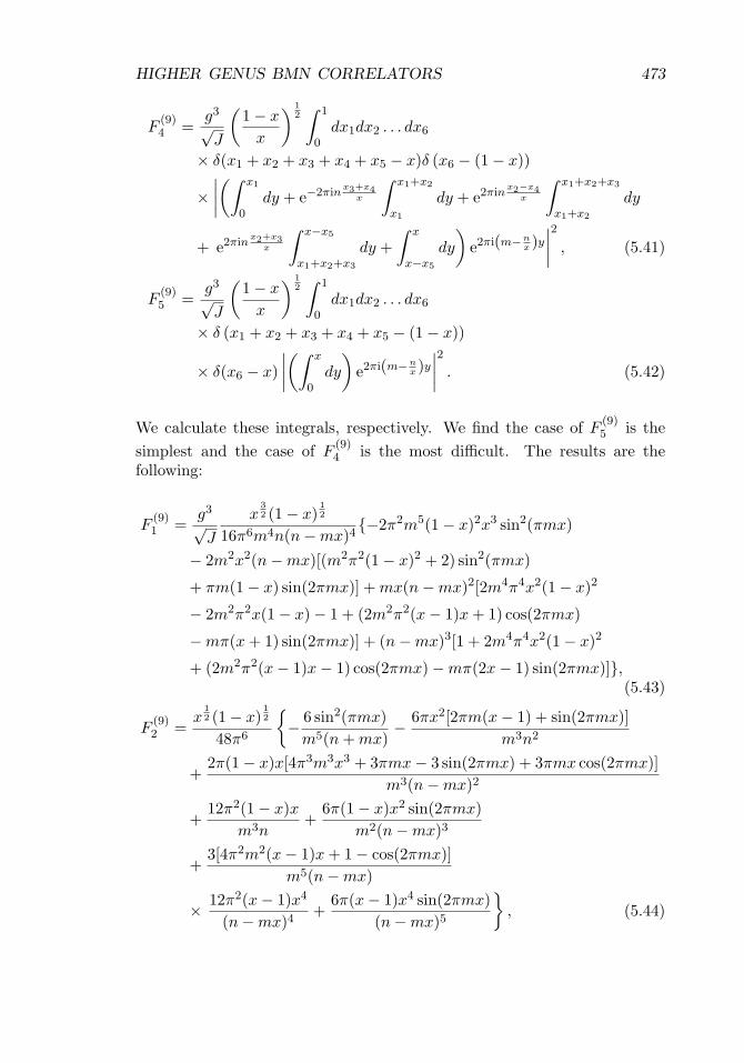
HIGHER GENUS BMN CORRELATORS 473
F(9)4 =
g3
√J
(1− x
x
) 12∫ 1
0dx1dx2 . . . dx6
× δ(x1 + x2 + x3 + x4 + x5 − x)δ (x6 − (1− x))
×∣∣∣∣(∫ x1
0dy + e−2πin
x3+x4x
∫ x1+x2
x1
dy + e2πinx2−x4
x
∫ x1+x2+x3
x1+x2
dy
+ e2πinx2+x3
x
∫ x−x5
x1+x2+x3
dy +∫ x
x−x5
dy
)e2πi(m−n
x )y
∣∣∣∣2
, (5.41)
F(9)5 =
g3
√J
(1− x
x
) 12∫ 1
0dx1dx2 . . . dx6
× δ (x1 + x2 + x3 + x4 + x5 − (1− x))
× δ(x6 − x)∣∣∣∣(∫ x
0dy
)e2πi(m−n
x )y
∣∣∣∣2
. (5.42)
We calculate these integrals, respectively. We find the case of F(9)5 is the
simplest and the case of F(9)4 is the most difficult. The results are the
following:
F(9)1 =
g3
√J
x32 (1− x)
12
16π6m4n(n−mx)4{−2π2m5(1− x)2x3 sin2(πmx)
− 2m2x2(n−mx)[(m2π2(1− x)2 + 2) sin2(πmx)
+ πm(1− x) sin(2πmx)] + mx(n−mx)2[2m4π4x2(1− x)2
− 2m2π2x(1− x)− 1 + (2m2π2(x− 1)x + 1) cos(2πmx)
−mπ(x + 1) sin(2πmx)] + (n−mx)3[1 + 2m4π4x2(1− x)2
+ (2m2π2(x− 1)x− 1) cos(2πmx)−mπ(2x− 1) sin(2πmx)]},(5.43)
F(9)2 =
x12 (1− x)
12
48π6
{− 6 sin2(πmx)
m5(n + mx)− 6πx2[2πm(x− 1) + sin(2πmx)]
m3n2
+2π(1− x)x[4π3m3x3 + 3πmx− 3 sin(2πmx) + 3πmx cos(2πmx)]
m3(n−mx)2
+12π2(1− x)x
m3n+
6π(1− x)x2 sin(2πmx)m2(n−mx)3
+3[4π2m2(x− 1)x + 1− cos(2πmx)]
m5(n−mx)
× 12π2(x− 1)x4
(n−mx)4+
6π(x− 1)x4 sin(2πmx)(n−mx)5
}, (5.44)

474 MIN–XIN HUANG
F(9)3 =
x52 (1− x)
12
24π6m3(mx− n)3{−2π4m4x4 + 6π4m4x3 − 6π4m4x2 + 2π4m4x
+ 2π4m3nx3 − 6π4m3nx2 + 6π4m3nx− 2π4m3n− 3π2m2x2
+ 3π2m2x + 3π2mnx− 3π2mn− 3 + π[π2m3(x− 1)3
+ m(6x− 3)− 3n] sin(2πmx) + [−3π2m2(x− 1)x
+ 3π2mn(x− 1) + 3] cos(2πmx)}, (5.45)
F(9)4 =
x12 (1− x)
12
96π6
{24 sin2(πmx)m5(mx + n)
+6x sin2(πmx)m4(mx + n)2
+6πx[2πmx + 3 sin(2πmx)]
m4n+
24πx2[πmx + sin(2πmx)]m3n2
+6x3[−5π2m2x2 + 3(π2m2x2 + 1) cos(2πmx)− 3]
m2(n−mx)4
+6[2π2m2x2 + 3πmx sin(2πmx)− 2 cos(2πmx) + 2]
m5(mx− n)
+
x[10π4m4x4 + (15− 2π4m4x4) cos(2πmx) + 12π2m2x2
+ 18πmx sin(2πmx)− 15]m4(n−mx)2
+4x2[πmx(2π2m2x2 + 3) sin(2πmx) + 6 cos(2πmx)− 6]
m3(mx− n)3
+60x5 sin2(πmx)
(n−mx)6+
24πx5 sin(2πmx)(n−mx)5
}, (5.46)
F(9)5 =
g3
√J
x32 (1− x)
92
sin(mπx)2
24π2(n−mx)2. (5.47)
Now we consider the string diagrams, which are obtained as decoration ofthe vacuum diagrams in figure 18 with stringy excitations. For the diagramsS
(7)1 , S
(7)2 , S
(7)3 and S
(7)5 , there is only one way to decoration, while for the
case of and S(7)4 there are 3 decorated diagrams. We depicted these diagrams
in figures 21, 22, 23. The contributions for diagrams in figure 21 are
S(9)1 = 2
∑k
〈OJ−m,mOJ
−k,k〉torus〈OJ−k,kO
J1−n,nOJ2〉,
S(9)2 = 2
∑k
〈OJ−m,mOJ1
−k,kOJ2〉〈OJ1
−k,kOJ1−n,n〉torus,
S(9)3 = 2〈OJ
−m,mOJ1−n,nOJ2〉〈OJ2OJ2〉torus, (5.48)

HIGHER GENUS BMN CORRELATORS 475
Figure 21: The decorated string diagrams of S(7)1 , S
(7)2 and S
(7)3 in figure 18.
We denote these contributions S(9)1 , S
(9)2 , S
(9)3 , respectively.
Figure 22: The decorated string diagrams of S(7)4 in figure 18. There are
three diagrams and we denote their contributions S(9)4,1 , S
(9)4,2 , S
(9)4,3 , respec-
tively and the total contributions by S(9)4 .
where the factor of 2 comes from the multiplicity of the one-loop stringpropagation diagram. Denoting the length of the intermediate operator inthe loop J3 = yJ and also J1 = xJ , we find the contributions of the diagramsin figures 22, 23 as the followings
S(9)4 = S
(9)4,1 + S
(9)4,2 + S
(9)4,3 , (5.49)
S(9)4,1 = 2
∫ x
0Jdy〈OJ
−m,mOyJ0 O
(1−y)J0 〉〈O(1−y)J
0 O(x−y)J0 O(1−x)J〉
× 〈O(x−y)J0 OyJ
0 OxJ−n,n〉,

476 MIN–XIN HUANG
Figure 23: The decorated string diagrams of S(7)5 in figure 18. There only
one diagram and we denote the contribution by S(9)5 .
S(9)4,2 =
∫ x
0Jdy
∑k
〈OJ−m,mOyJ
−k,kO(1−y)J〉〈O(1−y)JO(x−y)JO(1−x)J〉
× 〈O(x−y)JOyJ−k,kO
xJ−n,n〉,
S(9)4,3 =
∫ x
0Jdy
∑k
∑l
〈OJ−m,mOyJO
(1−y)J−k,k 〉〈O(1−y)J
−k,k O(x−y)J−l,l O(1−x)J〉
× 〈O(x−y)J−l,l OyJ
−k,kOxJ−n,n〉,
S(9)5 =
∫ 1
xJdy
∑k
〈OJ−m,mOyJ
−k,kO(1−y)J〉〈OyJ
−k,kO(y−x)JOxJ
−n,n〉
× 〈O(1−y)JO(y−x)JO(1−x)J〉, (5.50)
where the factor of 2 in S(9)4,1 is because there are two scalar insertion fields
in the BMN operator OJ−m,m, and we are using a slightly sloppy notationfor not distinguishing the different scalar insertions in the operators. Wecan choose any one for the operator OyJ
0 and the other one for O(1−y)J0 ,
and these two choices give the same contribution. We perform the sumsand integrals for the string diagrams contributions with the helps of thesummation formulae in Appendix A. The calculations for S
(9)4,3 is the most
difficult as it involves two sums over integers k and l, besides the integral of∫ x0 dy, and we find it best to do the sum over k first, then the sum over l
and the integral. We succeed in calculating the string diagrams analytically

HIGHER GENUS BMN CORRELATORS 477
and check the factorization relation
S(9)1 = 6F
(9)1 + 4
(F
(9)2 + F
(9)3
)+ 2
(F
(9)4 + F
(9)5
),
S(9)2 = 2F
(9)4 ,
S(9)3 = 2F
(9)5 ,
S(9)4 = 2F
(9)2 + 2F
(9)4 ,
S(9)5 = 2F
(9)3 + 2F
(9)5 .
5.4 Genus two correlators between two single trace operators
5.4.1 The vacuum diagrams and multiplicity
There are 3 string diagrams for the correlator 〈OJOJ〉genus 2, and we depictthem in figure 24. These diagrams are easy to calculate
S(10)1 =
(2〈OJOJ〉genus 1
)2=
g4
144,
S(10)2 =
∫ 1
0Jdx
x4g2
12〈OJOxJO(1−x)J〉〈OxJO(1−x)JOJ〉
=g4
504,
S(10)3 = J2
∫ 1
0dx
∫ x
0dy〈OJOxJO(1−x)J〉〈OyJO(1−y)JOJ〉
× 〈OxJOyJO(x−y)J〉〈O(1−x)JO(x−y)JO(1−y)J〉
=g4
280. (5.51)
For the calculations in field theory diagrams, we need to divide the singletrace into 8 segments, and there are 21 different diagrams, i.e., short pro-cesses, which are just permutations of (12 . . . 8). Here we will not drawthe diagrams again and simply use a permutation (a1a2 . . . a8) to repre-sent the field theory diagram, and denote their contributions F
(10)j with
j = 1, 2, . . . , 21. To derive the multiplicity of the string diagrams in figure 24,we can start with a string (12 . . . 8), and perform the splitting and joiningoperations according the string diagram. We keep the resulting long pro-cesses whose final states are irreducible from combining segments. Using

478 MIN–XIN HUANG
Figure 24: The string diagrams for vacuum operators at genus 2. There arethree diagrams and we denote their contributions S
(10)1 , S
(10)2 and S
(10)3 .
a computer, we can count the multiplicities of string diagrams, and we listthem in table 3. We do not list all the long processes here because that wouldtake too much space. The multiplicity matrix is mij where i = 1, 2, 3 denotethe string diagrams and j = 1, 2, . . . , 21 denote the field theory diagrams.The factorization relation (4.2) is
S(10)i =
21∑j=1
mijF(10)j , for i = 1, 2, 3 (5.52)
For the vacuum operator, each field diagram contribute F(10)j = g4
8! for anyj due to choices of dividing the single string into eight segments. We seethe contributions of the string diagrams in (5.51) agree with their respectivetotal multiplicities with respects to the 21 field theory diagrams times g4
8! ,consistent with the factorization relation. The total contribution to thecorrelator 〈OJOJ〉genus 2 of the string diagrams is proportional that of thefield theory diagrams with a factor of 24. So, we can write the correlator as
〈OJOJ〉genus 2 =21∑
j=1
F(10)j =
124
3∑i=1
S(10)i =
g4
1920. (5.53)

HIGHER GENUS BMN CORRELATORS 479
Table 3: The multiplicity matrix of string diagrams in figure 24 with respectto the 21 short processes. These short processes are permutations of(1, 2, . . . , 8), and we have used the cyclicality of the string to put the segment(1) in the first position.
mij S(10)1 S
(10)2 S
(10)3 Total
F(10)1 : (1,4,7,6,5,8,3,2) 8 8 8 24
F(10)2 : (1,5,8,3,7,6,4,2) 12 4 8 24
F(10)3 : (1,6,4,8,3,7,5,2) 16 2 6 24
F(10)4 : (1,7,5,4,8,3,6,2) 12 4 8 24
F(10)5 : (1,8,3,6,5,4,7,2) 8 8 8 24
F(10)6 : (1,4,3,2,5,8,7,6) 8 8 8 24
F(10)7 : (1,4,8,7,5,3,2,6) 12 4 8 24
F(10)8 : (1,4,8,6,3,2,7,5) 16 2 6 24
F(10)9 : (1,4,7,3,2,8,6,5) 12 4 8 24
F(10)10 : (1,8,7,2,5,4,3,6) 8 8 8 24
F(10)11 : (1,8,6,4,3,7,2,5) 12 4 8 24
F(10)12 : (1,7,4,3,8,6,2,5) 16 2 6 24
F(10)13 : (1,7,6,2,5,8,4,3) 12 4 8 24
F(10)14 : (1,7,3,6,2,8,5,4) 16 2 6 24
F(10)15 : (1,5,4,2,8,7,3,6) 12 4 8 24
F(10)16 : (1,6,5,2,8,4,7,3) 16 2 6 24
F(10)17 : (1,8,4,7,2,6,5,3) 12 4 8 24
F(10)18 : (1,5,8,4,2,7,6,3) 16 2 6 24
F(10)19 : (1,5,3,8,7,4,2,6) 16 2 6 24
F(10)20 : (1,8,5,3,7,2,6,4) 16 2 6 24
F(10)21 : (1,6,3,8,5,2,7,4) 24 0 0 24
Total 280 80 144
5.4.2 The stringy BMN operators
We consider the stringy case 〈OJ−m,mOJ−n,n〉genus 2. A systematic way to dothe field theory diagram calculations for higher genus single trace operatorswere described in [17]. We summarize the details in Appendix B. Basi-cally the calculations of summing over BMN phases of the scalar insertions

480 MIN–XIN HUANG
Figure 25: The decorated string diagrams for the first vacuum diagram S(10)1
in figure 24. This diagram is the paste of two torus diagrams and we denotethe contribution S
(11)1 .
can be expressed in terms of some standardized integrals, which can be cal-culated recursively. We denote the contribution of a genus 2 field theorydiagram by F
(11)j where j = 1, 2, . . . , 21, and we calculate the contribution
F(11)j respectively for all the j’s in computer using the formula (B.6).
For the string diagrams, we decorate the vacuum string diagrams infigure 24 with scalar insertions. We depict the decorations of the threestring diagrams in figures 25, 26, 27, and denote their contributions S
(11)1 ,
S(11)2 and S
(11)3 , respectively.
We discuss the calculations of the string diagrams. The diagram in fig-ure 25 can be calculated using the one-loop string propagation amplitude in(5.2) or (5.4), and we find
S(11)1 =
+∞∑k=−∞
4〈OJ−m,mOJ
−k,k〉torus〈OJ−k,kO
J−n,n〉torus (5.54)
=
⎧⎪⎪⎪⎪⎪⎪⎪⎪⎪⎪⎪⎪⎪⎪⎪⎪⎪⎪⎪⎪⎨⎪⎪⎪⎪⎪⎪⎪⎪⎪⎪⎪⎪⎪⎪⎪⎪⎪⎪⎪⎪⎩
g4
144, m = n = 0;
0, m = 0, n �= 0,
orn = 0, m �= 0;
g4
(451
256π8m8− 145
96π6m6+
740π4m4
− 1252π2m2
+71
45,360
), m = n �= 0;
g4
144π2m2
(31185
128π6m6− 1197
8π4m4+
1118π2m2
+ 1)
, m = −n �= 0;
g4P1
360π8m6n6(m− n)8(m + n)4, all other cases;

HIGHER GENUS BMN CORRELATORS 481
Figure 26: The decorated string diagrams for the first vacuum diagram S(10)2
in figure 24. We use a dash line in the third diagram to represent it as thepaste of one-loop cubic diagram with a tree level cubic vertex, where wecan use results from previous Section 5.3 without the need for the details ofthe one-loop cubic part of the diagram. We denote the contributions of thethree diagrams S
(11)2,1 , S
(11)2,2 and S
(11)2,3 .
where the numerator in the last case is
P1 = m16(10π6n6 + 42π4n4 − 210π2n2 + 315)−m15n(20π6n6 + 153π4n4
− 795π2n2 + 1260)− 3m14n2(10π6n6 + 17π4n4 + 125π2n2 − 210)
+ m13n3(80π6n6 + 459π4n4 − 2205π2n2 + 3780) + m12n4(20π6n6
− 174π4n4 + 3225π2n2 − 5310)− 3m11n5(40π6n6 + 102π4n4
− 795π2n2 + 855) + m10n6(20π6n6 + 366π4n4 − 2640π2n2 + 8865)
+ m9n7(80π6n6 − 306π4n4 − 1950π2n2 − 4815)− 6m8n8(5π6n6
+ 29π4n4 + 440π2n2 + 4080) + m7n9(−20π6n6 + 459π4n4
+ 2385π2n2 − 4815) + m6n10(10π6n6 − 51π4n4 + 3225π2n2 + 8865)
− 9m5n11(17π4n4 + 245π2n2 + 285) + 3m4n12(14π4n4 − 125π2n2
− 1770) + 15m3n13(53π2n2 + 252)− 210m2n14(π2n2 − 3)
− 1260mn15 + 315n16. (5.55)

482 MIN–XIN HUANG
Figure 27: The decorated string diagrams for the first vacuum diagram S(10)3
in figure 24. These diagrams can be obtained by pasting a one-loop cubicdiagram with a tree level cubic vertex. We do not need to draw the detailsin the one-loop cubic part of the diagram but simply use the results fromthe previous Section 5.3. We denote the contributions of the two diagramsS
(11)3,1 and S
(11)3,2 .
For the three diagrams in figure 26, the first two are easy to handle becausethe one-loop propagation of the non-stringy operator just contributes a fac-tor of (1−x)4
12 , and the calculations are
S(11)2,1 =
g2
12
∫ 1
0(1− x)4dx
∞∑k=−∞
〈OJ−m,mOxJ
−k,kO(1−x)J〉〈OxJ
−k,kO(1−x)JOJ
−n,n〉,
S(11)2,2 =
g2
6
∫ 1
0(1− x)4dx〈OJ
−m,mOxJ0 O
(1−x)J0 〉〈OxJ
0 O(1−x)J0 OJ
−n,n〉 (5.56)
where there is an extra factor of 2 in front of the second diagram S(11)2,2
because there are two choices for the scalar insertion in the operator O(1−x)J0
that undergoes one-loop propagation. For the third diagram S(11)2,3 in fig-
ure 26, it is much easier to use our previous results on one-loop cubic inter-actions. We divide the diagram into two part by a dash line and treat theone-loop cubic part on the left as a black box, which we have calculated

HIGHER GENUS BMN CORRELATORS 483
previously in the second equation in (5.48). We find
S(11)2,3 =
∫ 1
0Jdx
∞∑k=−∞
S(9)2 (m, k, x)〈OxJ
−k,kO(1−x)JOJ
−n,n〉. (5.57)
Putting the three contributions together we find the total contribution
S(11)2 = S
(11)2,1 + S
(11)2,2 + S
(11)2,3 (5.58)
=
⎧⎪⎪⎪⎪⎪⎪⎪⎪⎪⎪⎪⎪⎪⎪⎪⎪⎪⎪⎪⎪⎪⎪⎪⎪⎪⎨⎪⎪⎪⎪⎪⎪⎪⎪⎪⎪⎪⎪⎪⎪⎪⎪⎪⎪⎪⎪⎪⎪⎪⎪⎪⎩
g4
504, m = n = 0;
0, m = 0, n �= 0,
or n = 0, m �= 0;
g4
(1023
256π8m8− 21
16π6m6+
31240π4m4
− 1315π2m2
+1
2160
), m = n �= 0;
g4
504π2m2
(− 76,923
512π6m6− 12,789
64π4m4
+987
40π2m2+ 1
), m = −n �= 0;
g4P2
10, 080π8m6n6(m− n)8(m + n)4, all other cases;
where the numerator in the last case is
P2 = m16(80π6n6 + 546π4n4 − 4830π2n2 + 2520)−m15n(160π6n6
+ 1848π4n4 − 15,750π2n2 + 2835)− 15m14n2(16π6n6 + 28π4n4
− 210π2n2 + 945) + m13n3(640π6n6 + 5544π4n4 − 59,220π2n2
+ 17,955) + m12n4(160π6n6 − 3234π4n4 + 32,550π2n2 + 19,215)
− 3m11n5(320π6n6 + 1232π4n4 − 31430π2n2 + 5565)
+ m10n6(160π6n6 + 6216π4n4 − 30,870π2n2 − 7875)
+ m9n7(640π6n6 − 3696π4n4 − 10,1640π2n2 − 71,505)
− 6m8n8(40π6n6 + 539π4n4 + 5145π2n2 + 51,135)
+ m7n9(−160π6n6 + 5544π4n4 + 94,290π2n2 − 71,505)

484 MIN–XIN HUANG
+ 5m6n10(16π6n6 − 84π4n4 + 6510π2n2 − 1575)
− 21m5n11(88π4n4 + 2820π2n2 + 795) + 21m4n12(26π4n4
+ 150π2n2 + 915) + 315m3n13(50π2n2 + 57)
− 105m2n14(46π2n2 + 135)− 2835mn15 + 2520n16. (5.59)
For the two diagrams in figure 27, we also consider them as the pastings oftwo diagrams that we separate by a dash line. The left parts of the diagramshave been computed before in the last two equations of (5.37) and in (5.49,5.50), so we can treat them as a black box and simply use the previousresults. We note that in Section 5.3.3 we present the results for genericcase k �= 0, but here we also need to sum over the intermediate state withk = 0 in the second diagram S
(11)3,2 , which we have calculated separately. The
calculations go as the followings
S(11)3,1 =
∫ 1
0Jdx
[S
(8)4 (m, x) + S
(8)5 (m, x)
]〈OxJ
0 O(1−x)J0 OJ
−n,n〉,
S(11)3,2 =
∫ 1
0Jdx
∞∑k=−∞
[S
(9)4 (m, k, x) + S
(9)5 (m, k, x)
]〈OxJ
−k,kO(1−x)JOJ
−n,n〉
(5.60)
We find the total contribution
S(11)3 = S
(11)3,1 + S
(11)3,2 (5.61)
=
⎧⎪⎪⎪⎪⎪⎪⎪⎪⎪⎪⎪⎪⎪⎪⎪⎪⎪⎪⎪⎪⎪⎪⎪⎪⎪⎨⎪⎪⎪⎪⎪⎪⎪⎪⎪⎪⎪⎪⎪⎪⎪⎪⎪⎪⎪⎪⎪⎪⎪⎪⎪⎩
g4
280, m = n = 0;
0, m = 0, n �= 0,
or n = 0, m �= 0;
g4
(− 1045
256π8m8− 25
48π6m6+
748π4m4
− 1210π2m2
+37
45,360
), m = n �= 0;
g4
280π2m2
(− 199,815
512π6m6− 7665
64π4m4
+147
8π2m2+ 1
), m = −n �= 0;
g4P3
3360π8m6n6(m− n)8(m + n)4, all other cases;

HIGHER GENUS BMN CORRELATORS 485
where the numerator in the last case is
P3 = 2m16(24π6n6 + 133π4n4 − 735π2n2 − 1890) + m15(−96π6n7
− 896π4n5 + 4970π2n3 + 12,705n) + m14(−144π6n8 − 308π4n6
+ 770π2n4 + 1365n2) + 3m13n3(128π6n6 + 896π4n4 − 6580π2n2
− 15,855) + m12n4(96π6n6 − 1162π4n4 + 11,970π2n2 + 31,815)
+ m11n5(−576π6n6 − 1792π4n4 + 36,190π2n2 + 72,345)
+ m10n6(96π6n6 + 2408π4n4 − 11,270π2n2 − 75,075) + m9n7(384π6n6
− 1792π4n4 − 42,840π2n2 − 68,565)− 2m8n8(72π6n6 + 581π4n4
+ 5635π2n2 + 12,285) + m7n9(−96π6n6 + 2688π4n4 + 36,190π2n2
− 68,565) + m6n10(48π6n6 − 308π4n4 + 11,970π2n2 − 75,075)
− 7m5n11(128π4n4 + 2820π2n2 − 10,335) + 7m4n12(38π4n4
+ 110π2n2 + 4545) + 35m3n13(142π2n2 − 1359)
− 105m2n14(14π2n2 − 13) + 12,705mn15 − 3780n16. (5.62)
We check the factorization relation for the three groups of string diagramsin a computer
S(11)i =
21∑j=1
mijF(11)j , for i = 1, 2, 3. (5.63)
where the results of S(11)i are written in (5.54, 5.58, 5.61), the multiplicity
matrix mij can be found in table 3, and we have also computed the F(11)j
(j = 1, 2, . . . , 21) in computer according to the formula (B.6) but there aretoo many expressions (21 of them) to write down here. Again we can writethe total contributions to the genus two correlator as
〈OJ−m,mOJ
−n,n〉genus 2 =21∑
j=1
F(11)j =
124
3∑i=1
S(11)i . (5.64)
5.5 Genus three: a test
We consider the BMN correlator 〈OJ−m,mOJ−n,n〉genus 3. There are 11!!7 = 1485
different field diagrams represented by permutations of (1, 2, . . . , 12). We

486 MIN–XIN HUANG
calculate these 1485 diagrams in computer using the formula (B.6) simi-larly as in the previous section Denoting the contributions as F
(12)j , j =
1, 2, . . . , 1485, the total contribution to the correlator is
〈OJ−m,mOJ
−n,n〉genus 3 =1485∑j=1
F(12)j (5.65)
=
⎧⎪⎪⎪⎪⎪⎪⎪⎪⎪⎪⎪⎪⎪⎪⎪⎪⎪⎪⎪⎪⎪⎪⎪⎪⎪⎪⎪⎪⎪⎪⎪⎨⎪⎪⎪⎪⎪⎪⎪⎪⎪⎪⎪⎪⎪⎪⎪⎪⎪⎪⎪⎪⎪⎪⎪⎪⎪⎪⎪⎪⎪⎪⎪⎩
g6
322,560, m = n = 0;
0, m = 0, n �= 0,
or n = 0, m �= 0;g6
518,918,400
(8,856,072,225256π12m12
− 10,877,691,825128π10m10
m = n �= 0;
+1,949,592,645
64π8m8− 26,042,445
8π6m6
+927,3558π4m4
− 52394π2m2
+ 251)
,
g6
215,040π2m2
(− 2,807,805
512π10m10− 35,315
16π8m8+
155,28132π6m6
m = −n �= 0;
− 54618π4m4
+4151
216π2m2+ 1
),
g6P4(m,n)m10n10(m− n)12(m + n)8
, all other cases;
where P4(m, n) is a polynomial of m, n which is too long to write down here.
We test the factorization relation for a 3-loop string diagrams shown infigure 28. This diagram is one of simplest among 3-loop string diagrams andcan be calculated as the following:
S(12)1 = 8
+∞∑k=−∞
+∞∑l=−∞
〈OJ−m,mOJ
−k,k〉torus〈OJ−k,kO
J−l,l〉torus〈OJ
−l,lOJ−n,n〉torus
= 2+∞∑
k=−∞〈OJ
−m,mOJ−k,k〉torus S
(11)1 (k, n), (5.66)
where the formula for the torus two point function can be found in (5.2),and we can utilize the previous result S
(11)1 (k, n) in (5.54) of two-loop string
propagation for parts of the calculations.

HIGHER GENUS BMN CORRELATORS 487
Figure 28: A 3-loop string diagram for 〈OJ−m,mOJ−n,n〉genus 3. We denote its
contribution by S(12)1 . We test the factorization relation for this diagram.
Table 4: The multiplicities of the string diagram in figure 28 with respectto some samples of the 1485 short processes, which are permutations of(1, 2, . . . , 12), and we have used the cyclicality of the string to put thesegment (1) in the first position.
j = 1, 2, . . . , 1485 m1j for S(12)1
(1,4,7,6,5,8,11,10,9,12,3,2) 48(1,4,7,11,10,8,6,5,9,12,3,2) 72(1,4,7,11,9,6,5,10,8,12,3,2) 96(1,4,7,10,6,5,11,9,8,12,3,2) 72(1,4,7,10,9,8,11,6,5,12,3,2) 48(1,4,11,10,5,8,7,6,9,12,3,2) 48(1,4,11,9,7,6,10,5,8,12,3,2) 72(1,4,10,7,6,11,9,5,8,12,3,2) 96(1,4,10,9,5,8,11,7,6,12,3,2) 72(1,4,11,6,9,8,7,10,5,12,3,2) 48· · · · · ·· · · · · ·Total 277,200
We also use a computer to find the multiplicities of the string diagram infigure 28 with respect to the 1485 field theory diagrams, similarly as in theprevious case of genus 2. It turns out the multiplicity is non-vanishing withrespect to all 1485 diagrams. Obviously we can not list all the multiplicitieshere. We provide a small sample in table 4.
Denoting the contribution of a field theory diagram by F(12)j where j =
1, 2, . . . , 1485, the factorization relation for the string diagram in figure 28states that
S(12)1 =
1485∑j=1
m1jF(12)j . (5.67)

488 MIN–XIN HUANG
We calculate both the left hand side and the right hand side analytically,and check the factorization relation with the following result
S(12)1 =
1485∑j=1
m1jF(12)j (5.68)
=
⎧⎪⎪⎪⎪⎪⎪⎪⎪⎪⎪⎪⎪⎪⎪⎪⎪⎪⎪⎪⎪⎪⎪⎪⎪⎪⎪⎪⎪⎪⎪⎨⎪⎪⎪⎪⎪⎪⎪⎪⎪⎪⎪⎪⎪⎪⎪⎪⎪⎪⎪⎪⎪⎪⎪⎪⎪⎪⎪⎪⎪⎪⎩
g6
1728, m = n = 0;
0, m = 0, n �= 0,
or n = 0, m �= 0;g6
926,640
(73,345,119,7051024π12m12
− 1,955,422,75564π10m10
m = n �= 0;
+397,910,799
64π8m8− 33,182,721
56π6m6
+176,8918π4m4
− 510928π2m2
+ 83)
,
g6
1152π2m2
(90,781,1191024π10m10
− 4,409,493128π8m8
+486,81980π6m6
m = −n �= 0;
− 147,149280π4m4
+34,583
2520π2m2+ 1
),
g6P5(m, n)m10n10(m− n)12(m + n)8
, all other cases;
where P5(m, n) is a polynomial of m, n too long to write down here.
The sums and integrals in both the string diagrams and the field theorydiagrams become more and more difficult to do analytically as we go up ingenus and also include multi-trace operators. But it is certainly possibleto check the factorization relation further numerically since all sums andintegrals are convergent in this paper.
6 Correlators of BMN operators with more stringy modes
In the previous sections we considered correlators of BMN operators withat most two excitations, where the first stringy mode can appear due to theclosed string level matching condition. One can certainly add more stringymodes to the BMN operators, which corresponds to more field insertions inthe trace operators with phases. One can also consider the case that someof the scalar insertions are identical, which we do not expect to make a qual-itative change to the factorization rules. To illustrate that the factorization

HIGHER GENUS BMN CORRELATORS 489
relation also works for these cases, in this section we study some correlatorsinvolving BMN operators with three different scalar insertions.
6.1 The operator and vertices
We use three different scalar fields φ1, φ2 and φ3 to insert into the singletrace operator OJ = Tr(ZJ) with phases. The resulting properly normalizedBMN operator is
OJ(m1,m2,m3) =
1√NJ+2J
J−1∑l1,l2=0
e2πim2l1
J e2πim3l2
J Tr
×(φ1Z l1φ2Z l2−l1φ3ZJ−l2
), (6.1)
where the integers mi’s satisfy the level matching condition m1 + m2 + m3 =0, and we have used the cyclicality of the trace to put the scalar φ1 in thefirst positions. Similar to the case of two excitations, the summing overthe position of φ1 make the operator vanish if the level matching conditionm1 + m2 + m3 = 0 is not satisfied. From now on we use a subscript todenote the string modes when confusion may arise. For example, we denotethe BMN operator with two excited modes as OJ
(−n,n)(1,3)with the scalar
insertions of modes −n and n from φ1 and φ3. For the BMN operator withthree string modes this is not necessary since there is no confusion.
It is straightforward to compute the vertices with the operator (6.1) bysumming over the scalar insertions into diagram in figure 2 with phases. Wefind the vertices
〈OJ(m1,m2,m3)O
xJ(−n,n)(1,2)
O(1−x)J(0)3
〉
= − g√J
x32sin(πm1x) sin(πm2x) sin(πm3x)
π3m3(m1x + n)(m2x− n),
〈OJ(m1,m2,m3)O
xJ(n1,n2,n3)O
(1−x)J〉
=g√J
x2(1− x)12
sin(πm1x) sin(πm2x) sin(πm3x)π3(m1x− n1)(m2x− n2)(m3x− n3)
. (6.2)
The above correlators are valid as long as the denominator is not zero.For the special cases when the denominator vanishes, we have the

490 MIN–XIN HUANG
Figure 29: The field theory diagrams for the correlators〈OJ
(m1,m2,m3)Ox1J(0)1
Ox2J(0)2
Ox3J(0)3〉. We denote the contributions F
(13)1 , F
(13)2
and F(13)3 .
following correlators:
〈OJ(−m,m,0)O
xJ(−n,n)(1,2)
O(1−x)J(0)3
〉 =g√J
x32 (1− x)
sin2(πmx)π2(mx− n)2
,
〈OJ(0,−m,m)O
xJ(0,0)(1,2)
O(1−x)J(0)3
〉 = − g√J
x12sin2(πmx)
π2m2,
〈OJ(0,0,0)O
xJ(0,0)(1,2)
O(1−x)J(0)3
〉 =g√J
x32 (1− x),
〈OJ(−m,m,0)O
xJ(−n,n,0)O
(1−x)J〉 =g√J
x2(1− x)12
sin2(πmx)π2(mx− n)2
,
〈OJ(0,0,0)O
xJ(0,0,0)O
(1−x)J〉 =g√J
x2(1− x)12 . (6.3)
6.2 The case of 〈OJ(m1,m2,m3)
Ox1J(0)1
Ox2J(0)2
Ox3J(0)3
〉
We study a simple case of the correlator 〈OJ(m1,m2,m3)O
x1J(0)1
Ox2J(0)2
Ox3J(0)3〉 to
illustrate the factorization relation with more than 2 stringy mode exci-tations. It is implicit that the parameters satisfy m1 + m2 + m3 = 0 andx1 + x2 + x3 = 1. The field theory diagrams are basically the same as thecase of two string modes in figures 3, 5 and we draw them in figure 29.

HIGHER GENUS BMN CORRELATORS 491
Figure 30: The string diagrams for the correlators 〈OJ(m1,m2,m3)
Ox1J(0)1
Ox2J(0)2
Ox3J(0)3〉. We denote the contributions S
(13)1 , S
(13)2 and S
(13)3 .
We calculate the contributions by summing over the three scalar insertionswith phases.
F(13)1 =
g2
J
∫ x1
0dy1
(∫ y1
0+∫ x1+x2
y1+x2
)dy2 e−2πim1y2
∫ y1+x2
y1
dy3 e−2πim2y3
×∫ 1
x1+x2
dy4 e−2πim3y4 =sin(m2x2π) sin(m3x3π)
2π4m1m22m
23
× {m1 cos[π(m2x2 −m3x3)],
+ (−1)m2m3 cos[π(m1x3 + m2x1)]
+ (−1)m3m2 cos[π(m1x2 + m3x1)]}F
(13)2 = F
(13)1 (x1 ↔ x2, m1 ↔ m2),
F(13)3 = F
(13)1 (x1 ↔ x3, m1 ↔ m3). (6.4)
For the string diagrams, we draw them in figure 30. we calculate thediagrams using the vertices and summing over intermediate states
S(13)1 =
∞∑n=−∞
〈OJ(m1,m2,m3)O
(1−x1)J(−n,n)(2,3)
Ox1J(0)1〉〈O(1−x1)J
(−n,n)(2,3)Ox2J
(0)2Ox3J
(0)3〉,
S(13)2 = S
(13)1 (x1 ↔ x2, m1 ↔ m2),
S(13)3 = S
(13)1 (x1 ↔ x3, m1 ↔ m3). (6.5)
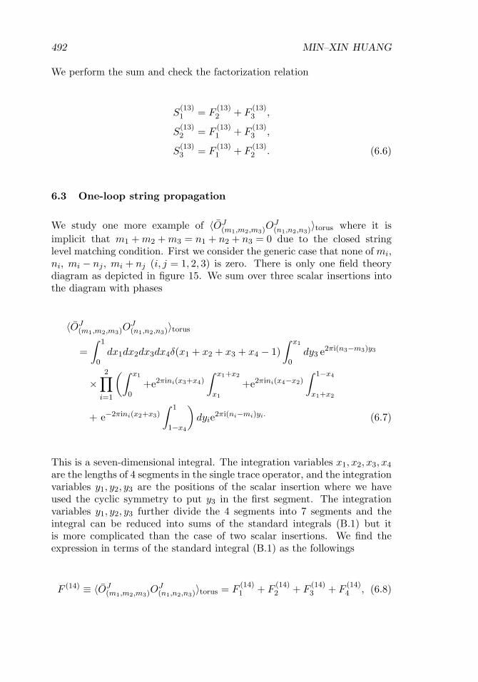
492 MIN–XIN HUANG
We perform the sum and check the factorization relation
S(13)1 = F
(13)2 + F
(13)3 ,
S(13)2 = F
(13)1 + F
(13)3 ,
S(13)3 = F
(13)1 + F
(13)2 . (6.6)
6.3 One-loop string propagation
We study one more example of 〈OJ(m1,m2,m3)O
J(n1,n2,n3)〉torus where it is
implicit that m1 + m2 + m3 = n1 + n2 + n3 = 0 due to the closed stringlevel matching condition. First we consider the generic case that none of mi,ni, mi − nj , mi + nj (i, j = 1, 2, 3) is zero. There is only one field theorydiagram as depicted in figure 15. We sum over three scalar insertions intothe diagram with phases
〈OJ(m1,m2,m3)O
J(n1,n2,n3)〉torus
=∫ 1
0dx1dx2dx3dx4δ(x1 + x2 + x3 + x4 − 1)
∫ x1
0dy3 e2πi(n3−m3)y3
×2∏
i=1
(∫ x1
0+e2πini(x3+x4)
∫ x1+x2
x1
+e2πini(x4−x2)
∫ 1−x4
x1+x2
+ e−2πini(x2+x3)
∫ 1
1−x4
)dyie2πi(ni−mi)yi. (6.7)
This is a seven-dimensional integral. The integration variables x1, x2, x3, x4
are the lengths of 4 segments in the single trace operator, and the integrationvariables y1, y2, y3 are the positions of the scalar insertion where we haveused the cyclic symmetry to put y3 in the first segment. The integrationvariables y1, y2, y3 further divide the 4 segments into 7 segments and theintegral can be reduced into sums of the standard integrals (B.1) but itis more complicated than the case of two scalar insertions. We find theexpression in terms of the standard integral (B.1) as the followings
F (14) ≡ 〈OJ(m1,m2,m3)O
J(n1,n2,n3)〉torus = F
(14)1 + F
(14)2 + F
(14)3 + F
(14)4 , (6.8)

HIGHER GENUS BMN CORRELATORS 493
where
F(14)1 ≡
∑i�=j
I(1,1,5)(2πi(mi − ni),−2πi(mj − nj), 0),
F(14)2 ≡
∑i�=j
I(1,2,2,2)(2πi(mi − ni),−2πi(mj − nj),−2πimj , 0),
+ I(1,2,2,2)(2πi(mi − ni),−2πi(mj − nj), 2πinj , 0),
F(14)3 ≡
∑i�=j
I(1,1,1,2,2)(2πi(mi − ni),−2πimj , 2πinj ,−2πi(mj − nj), 0),
F(14)4 ≡
∑i�=j
I(1,1,1,1,1,1,1)(2πimi, 2πini,−2πimj ,−2πinj ,
× 2πi(mi − nj),−2πi(mj − ni), 0). (6.9)
For the generic case of mi, ni, it turns out that F(14)2 = F
(14)3 = F
(14)4 = 0.
There seems to be some hidden symmetries which are not obvious the inte-gral expression (B.1). The contribution vanishes for each term in F
(14)4 , but
only the total contributions vanish in the cases F(14)2 and F
(14)3 . So the only
non-vanishing contribution is F(14)1 and we find the correlator
〈OJ(m1,m2,m3)O
J(n1,n2,n3)〉torus =
∑3i=1(mi − ni)2
32π4∏3
i=1(mi − ni)2. (6.10)
We consider the string diagrams. The two diagrams are drawn in figure 31and we denote the contributions S
(14)1 and S
(14)2 . The computations are
carried out by summing over the intermediate states
S(14)1 =
3∑i3=1
∫ 1
0Jdx
∞∑k=−∞
〈OJ(m1,m2,m3)O
xJ(−k,k)(i1,i2)
O(1−x)J(0)i3
〉
× 〈OxJ(−k,k)(i1,i2)
O(1−x)J(0)i3
OJ(n1,n2,n3)〉
S(14)2 =
∫ 1
0Jdx
∑k1+k2+k3=0
〈OJ(m1,m2,m3)O
xJ(k1,k2,k3)O
(1−x)J〉
× 〈OxJ(k1,k2,k3)O
(1−x)JOJ(n1,n2,n3)〉 (6.11)
We perform the the sums and integrals for the contributions. It turns out forthe generic case of mi, ni, the first diagram vanishes S
(14)1 = 0. The vanishing
is due to an antisymmetry x→ 1− x of the integrand, which is not presentat the vertex level, but only appears after summing over the string modes

494 MIN–XIN HUANG
Figure 31: The string diagrams for the correlators 〈OJ(m1,m2,m3)
OJ(n1,n2,n3)〉torus, where there are 3 cases for the first diagrams
(i1, i2, i3) = (1, 2, 3), (2, 3, 1), (3, 1, 2). We denote the contributions ofthese 2 diagrams S
(14)1 and S
(14)2 .
k of the intermediate states. So the total contribution S(14) ≡ S(14)1 + S
(14)2
only come from the second diagram S(14)2 . We do the calculations and check
the factorization relation with the field theory contribution (6.10),
S(14) = 2〈OJ(m1,m2,m3)O
J(n1,n2,n3)〉torus =
∑3i=1(mi − ni)2
16π4∏3
i=1(mi − ni)2(6.12)
The formulae (6.10) for the correlator is valid for the generic case whenthe arguments in the (6.9) are not degenerate. When some arguments areidentical, we need to combine them according to (B.2) before we can use(B.4, B.5) to compute them. It can be easily checked that the degener-acy only happens when some of the mi, ni, mi − nj , mi + nj (i, j = 1, 2, 3)vanish. We discuss these various cases in the followings. Needless to say,one can check that the factorization relation S(14) = 2F (14) is fulfilled for allthese cases.
1) mi = 0, ni �= 0 or mi �= 0, ni = 0 for some i ∈ {1, 2, 3}. We find thecorrelator vanish F (14) = 0 regardless whether there are further degen-eracies in the other parameters. The vanishing can be directly seenfrom the integral (6.7). For example, if n1 = 0 and m1 �= 0, then oneintegral contributes a factor
∫ 10 dy1e
−2πim1y1 = 0. For the string dia-grams, we find both S
(14)1 and S
(14)2 no longer vanish but their contri-
butions cancel each others.

HIGHER GENUS BMN CORRELATORS 495
2) mi = ni = 0 for some i ∈ {1, 2, 3}. The correlator reduces to the case ofcorrelator with 2 scalar insertions (5.2) studied before, since there is nophase factor in summing over the scalar insertion φi and it contributesjust a constant factor which is properly cancelled.
3) n3 = m3 (without loss of generality) and everything else generic. Thelevel matching conditions are m2 = −m1 −m3, n2 = −n1 − n3, andwe can express the correlator using three parameters m1, n1, m3. Inthis case we find all F
(14)i (i = 1, 2, 3, 4) in (6.9) are non-vanishing, and
the answer looks more complicated than the generic case
F (14) =1
48π2(m1 − n1)2+
116π4(m1 − n1)4
− m43 + (m1 + n1)m3
3 + m1n1m23 −m1n1(m1 + n1)m3 −m2
1n21
16π4(m1 − n1)2m1n1m23(m3 + m1)(m3 + n1)
+1
16π4(m1 − n1)2m21n
21m
23(m3 + m1)2(m3 + n1)2
{m63(m
21 + n2
1)
+ 2m53(m
21n1 + m1n
21 + m3
1 + n31) + m4
3(4m31n1 + 2m2
1n21
+ 4m1n31 + m4
1 + n41) + 2m3
3m1n1(m31 + n3
1)− 8m23m
31n
31
− 4m3m31n
31(m1 + n1)− 2m4
1n41}. (6.13)
4) n3 = m2 (without loss of generality) and everything else generic. Itturns out in this case the generic formula (6.10) is still valid eventhough some arguments in (6.9) are degenerate. One can simply plugin the parameters with n3 = m2.
5) n3 = −m3 (without loss of generality) and everything else generic. Itturns out in this case the generic formula (6.10) is also still valid eventhough some arguments in (6.9) are degenerate.
6) n3 = −m2 (without loss of generality) and everything else generic. Thecorrelator is different from the generic formula. We find
F (14) =2m2
1 − 3m1n1 + 2n21
16π4m21n
21(m1 − n1)2
. (6.14)
We note that there are three free parameters after taking into accountthe level matching conditions, but the correlator only depends on twoparameters.
7) n3 = m3, n2 = m2 (without loss of generality) and everything elsegeneric. The level match conditions also require n1 = m1. We findthe correlator
F (14) =1
120+
516π4
(1
m41
+1
m42
+1
m43
)−(m2
1 + m22 + m2
3
)2192π2m2
1m22m
23
. (6.15)

496 MIN–XIN HUANG
8) n3 = m3, n2 = m1 (without loss of generality) and everything elsegeneric. The level match conditions also require n1 = m2. We findthe correlator
F (14) =1
48π4m21n
21(m1 − n1)4(m1 + n1)2
[9(m61 + n6
1)− 12m1n1(m41 + n4
1)
− 9m21n
21(m
21 + n2
1) + 36m31n
31 − π2m2
1n21(m1 − n1)2]. (6.16)
We note that we would get an incorrect result by simply setting m3 =−m1 −m2 = −m1 − n1 in (6.13), though there is no apparent singu-larity in doing so. In other words, the condition n2 = m1 generatesmore degeneracies and further modifies the result.
9) n3 = m2, n2 = m1 (without loss of generality) and everything elsegeneric. The level match conditions also require n1 = m3. In thiscase, the generic formula (6.10) is valid.
10) n3 = −m3, n2 = −m2 (without loss of generality) and everything elsegeneric. The level match conditions also require n1 = −m1. In thiscase, the generic formula (6.10) is valid.
11) n3 = −m2, n2 = −m3 (without loss of generality) and everything elsegeneric. The level match conditions also force n1 = −m1. In this case,the generic formula (6.10) is not valid, and we find
F (14) =15
64π4m41
. (6.17)
We note that this can not be obtained from the more generic formula(6.14) for the case of n3 = −m2 by further setting n1 = −m1.
12) n3 = −m2, n2 = −m1 (without loss of generality) and everything elsegeneric. The level match conditions also force n1 = −m3. In this casethe generic formula (6.10) is not valid, and we find
F (14) =m2
1 −m1n1 + n21
4π4m21n
21(m1 − n1)2
. (6.18)
This is also different from the more generic formula (6.14).13) n3 = m3, n2 = −m2 (without loss of generality) and everything else
generic. In this case the correlator can be obtained from the caseof n3 = m3 discussed above by further setting n2 = −m2 in (6.13).In other words, the condition n2 = −m2 does not further change thecorrelator through degeneracies.
14) n3 = m3, n2 = −m1 (without loss of generality) and everything elsegeneric. In this case the correlator can not be obtained from the pre-vious case of n3 = m3 by further setting n2 = −m1. In other words,

HIGHER GENUS BMN CORRELATORS 497
the condition n2 = −m1 changes the correlator through more degen-eracies in the integral. We find the correlator
F (14) =3m6
1 + 3m21m
43 + 6m6
3 + π2m21m
23
(m2
1 −m23
)248π4m2
1m43
(m2
1 −m23
)2 . (6.19)
15) n3 = −m3, n2 = m1 (without loss of generality) and everything elsegeneric. In this case the generic formula (6.10) is valid.
16) n3 = −m2, n2 = m3 or n2 = m1 (without loss of generality) and every-thing else generic. In this case the correlator can be obtained from themore generic previous case of n3 = −m2 (6.14). In fact, the conditionn2 = m3 or n2 = m1 does not change the correlator at all, since theformula (6.14) only depends on two parameters m1 and n1.
One general pattern in these discussions is that the degeneracies mi =−ni and mi = nj (i �= j) are more benign than the other cases of mi = ni
and mi = −nj (i �= j), and one can often obtain the correlator by directlyplugging these benign conditions in the formula of a more generic case.There is only one exception to this pattern encountered in case 8 where thecondition n2 = m1 does modify the formula for the correlator from a moregeneric situation.
It is also possible to derive the factorization relation S(14) = 2F (14) usingthe integral form of the vertices as we did in Section 5.2 for BMN operatorswith two stringy modes. This would be much more complicated than theprevious case but the derivation would apply to all the degenerate caseswithout the need to discuss each case separately.
7 Conclusion
In this paper, we check the factorization relation (4.2) in many exampleswhere the initial state is a single string state. However, we expect thefactorization to also work for certain string diagrams in the cases whereboth initial and final states are multi-string states, so long as no string in theintermediate steps of the string diagram is longer than all the external initialand final strings in terms of the number of Z fields in the correspondingtrace operator. This is supported by the study of tree level 2→ 2 processin Section 3.2, where we find the factorization works for T, U channels, butfails for the S channel because the string propagating in the S channel isthe longest string.
It is well known that in flat Minkowski space, the string amplitude ath-loop level goes like (2h)!g2h
s for large h, while the Yang–Mills field theory

498 MIN–XIN HUANG
amplitude goes like h!g2hY M , where gs and gY M are the coupling constants
of the string theory and field theory. The perturbation theory is divergentbut is Borel summable. There is an ambiguity in performing the Borelsummation of asymptotic series, which is of the order e−A/gs for string theoryand e−A/g2
Y M , where A represents a positive number. These ambiguitiescome from non-perturbative effects not captured by the perturbation theory,and they come from D-branes in the case of string theory and instantonsin the case of gauge theory. In our case, the effective coupling constant isg = J2
N . At genus h level, there are (4h−1)!!2h+1 field theory diagrams [22]. For
the vacuum operator each diagram contributes 1/(4h)!, so the perturbationseries is actually convergent and can be summed up
〈OJOJ〉 =∞∑
h=0
(4h− 1)!!(2h + 1)(4h)!
g2h =2 sinh(g/2)
g. (7.1)
We do not expect a qualitative change to convergence property for the cor-relators of general stringy BMN operators. To explain the convergence, wenote that in the free field limit λ′ = 0, we effectively “zoom in” an infinites-imal patch of the spacetime where the corresponding string theory lives, sothat the spacetime becomes infinitely curved and the strings are infinitelylong. We conjecture that in this limit we have decoupled the D-branes andtheir non-perturbative effects, so the string perturbation theory is completeand convergent.
Appendix A Some useful summation formulae
Some useful summation formulae for many of the calculations of string dia-grams is
∞∑p=−∞
1(p− α1)(p− α2)
= −πcot(α1π)− cot(α2π)
α1 − α2,
∞∑p=−∞
sin2(pπβ)(p− α1)(p− α2)
=π
(α1 − α2)
[sin(α1π(1− β)) sin(α1πβ)
sin(α1π)
− sin(α2π(1− β)) sin(α2πβ)sin(α2π)
], (A.1)
∞∑p=−∞
sin(2pπβ)(p−α1)(p−α2)
=π
(α1−α2)
[sin(α1π(1− 2β))
sin(α1π)− sin(α2π(1− 2β))
sin(α2π)
].
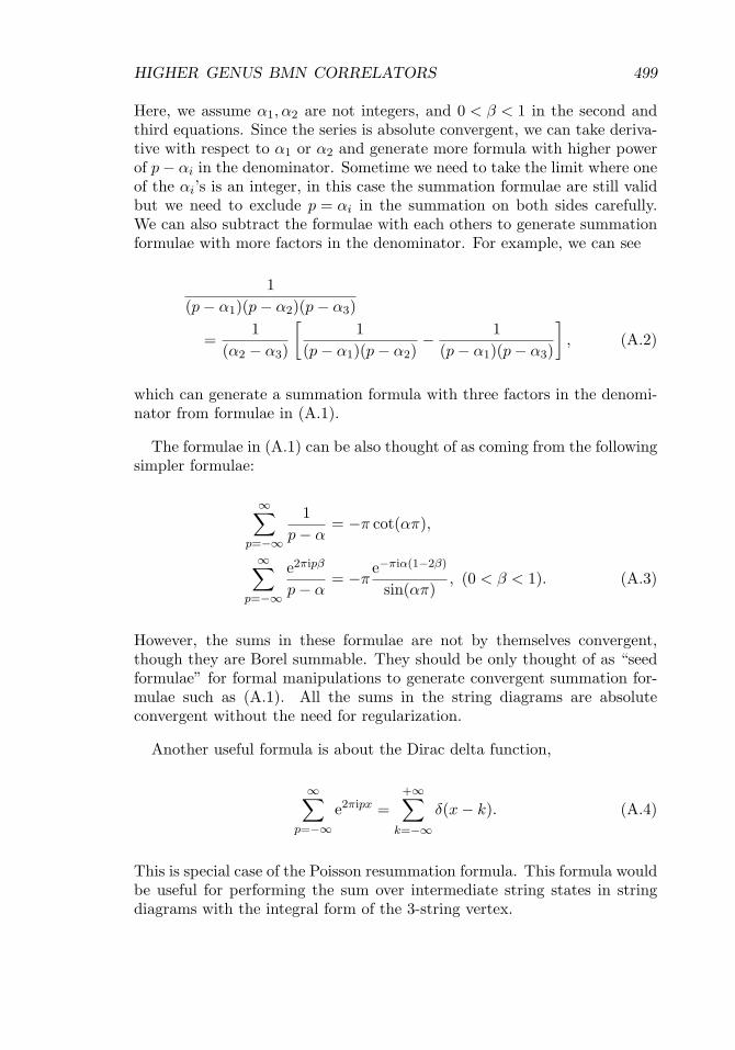
HIGHER GENUS BMN CORRELATORS 499
Here, we assume α1, α2 are not integers, and 0 < β < 1 in the second andthird equations. Since the series is absolute convergent, we can take deriva-tive with respect to α1 or α2 and generate more formula with higher powerof p− αi in the denominator. Sometime we need to take the limit where oneof the αi’s is an integer, in this case the summation formulae are still validbut we need to exclude p = αi in the summation on both sides carefully.We can also subtract the formulae with each others to generate summationformulae with more factors in the denominator. For example, we can see
1(p− α1)(p− α2)(p− α3)
=1
(α2 − α3)
[1
(p− α1)(p− α2)− 1
(p− α1)(p− α3)
], (A.2)
which can generate a summation formula with three factors in the denomi-nator from formulae in (A.1).
The formulae in (A.1) can be also thought of as coming from the followingsimpler formulae:
∞∑p=−∞
1p− α
= −π cot(απ),
∞∑p=−∞
e2πipβ
p− α= −π
e−πiα(1−2β)
sin(απ), (0 < β < 1). (A.3)
However, the sums in these formulae are not by themselves convergent,though they are Borel summable. They should be only thought of as “seedformulae” for formal manipulations to generate convergent summation for-mulae such as (A.1). All the sums in the string diagrams are absoluteconvergent without the need for regularization.
Another useful formula is about the Dirac delta function,
∞∑p=−∞
e2πipx =+∞∑
k=−∞δ(x− k). (A.4)
This is special case of the Poisson resummation formula. This formula wouldbe useful for performing the sum over intermediate string states in stringdiagrams with the integral form of the 3-string vertex.
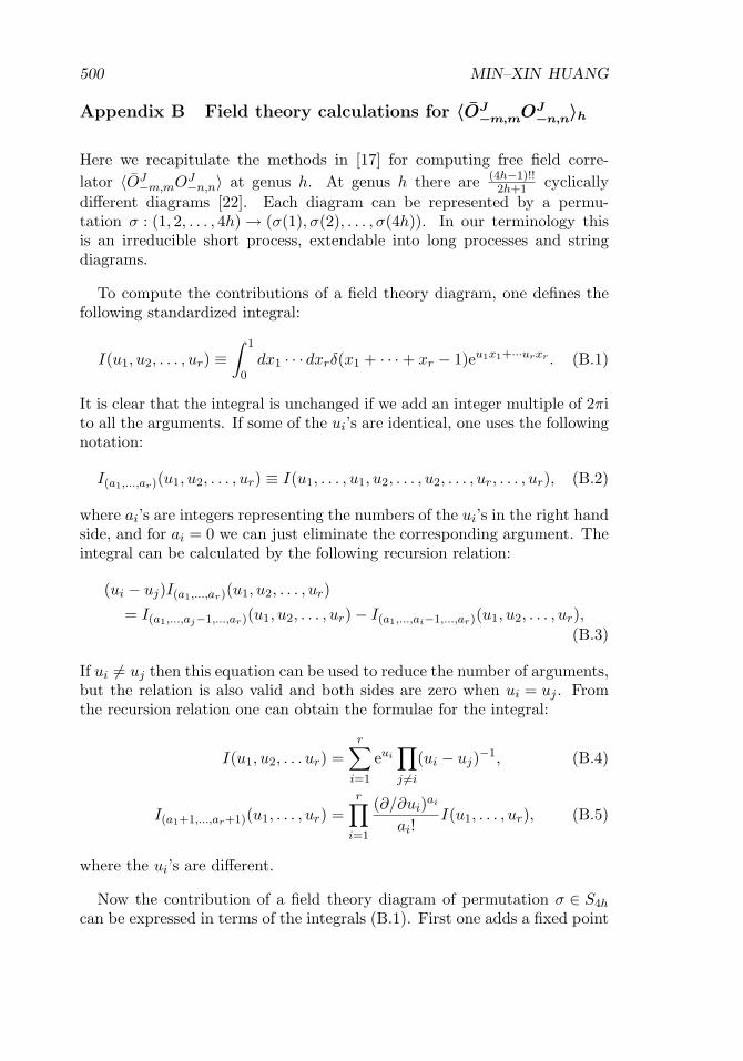
500 MIN–XIN HUANG
Appendix B Field theory calculations for 〈OJ−m,mOJ
−n,n〉h
Here we recapitulate the methods in [17] for computing free field corre-lator 〈OJ−m,mOJ−n,n〉 at genus h. At genus h there are (4h−1)!!
2h+1 cyclicallydifferent diagrams [22]. Each diagram can be represented by a permu-tation σ : (1, 2, . . . , 4h)→ (σ(1), σ(2), . . . , σ(4h)). In our terminology thisis an irreducible short process, extendable into long processes and stringdiagrams.
To compute the contributions of a field theory diagram, one defines thefollowing standardized integral:
I(u1, u2, . . . , ur) ≡∫ 1
0dx1 · · · dxrδ(x1 + · · ·+ xr − 1)eu1x1+···urxr . (B.1)
It is clear that the integral is unchanged if we add an integer multiple of 2πito all the arguments. If some of the ui’s are identical, one uses the followingnotation:
I(a1,...,ar)(u1, u2, . . . , ur) ≡ I(u1, . . . , u1, u2, . . . , u2, . . . , ur, . . . , ur), (B.2)
where ai’s are integers representing the numbers of the ui’s in the right handside, and for ai = 0 we can just eliminate the corresponding argument. Theintegral can be calculated by the following recursion relation:
(ui − uj)I(a1,...,ar)(u1, u2, . . . , ur)
= I(a1,...,aj−1,...,ar)(u1, u2, . . . , ur)− I(a1,...,ai−1,...,ar)(u1, u2, . . . , ur),(B.3)
If ui �= uj then this equation can be used to reduce the number of arguments,but the relation is also valid and both sides are zero when ui = uj . Fromthe recursion relation one can obtain the formulae for the integral:
I(u1, u2, . . . ur) =r∑
i=1
eui∏j �=i
(ui − uj)−1, (B.4)
I(a1+1,...,ar+1)(u1, . . . , ur) =r∏
i=1
(∂/∂ui)ai
ai!I(u1, . . . , ur), (B.5)
where the ui’s are different.
Now the contribution of a field theory diagram of permutation σ ∈ S4h
can be expressed in terms of the integrals (B.1). First one adds a fixed point

HIGHER GENUS BMN CORRELATORS 501
4h + 1 to the permutation σ to obtain another permutation σ ∈ S4h+1, andfor 1 ≤ i ≤ 4h + 1 one defines the following numbers:
lli(σ) = number of {j | j < i, σ(j) < σ(i)},lri(σ) = number of {j | j < i, σ(j) > σ(i)},rli(σ) = number of {j | j > i, σ(j) < σ(i)},rri(σ) = number of {j | j > i, σ(j) > σ(i)},
then the contribution of a field theory diagram represented by permutationσ to the correlator 〈OJ−m,mOJ−n,n〉h can be expressed as
Fσ(m, n) =4h+1∑i=1
I(lli(σ)+1,lri(σ),rli(σ),rri(σ)+1)
× (2πi(m− n), 2πim,−2πin, 0). (B.6)
To understand this formula, we note that since lli(σ) + lri(σ) + rli(σ) +rri(σ) = 4h, this is a 4h + 2 dimensional integral with r = 4h + 2 in termsof (B.1). The integration variables come from the division of the singletrace into 4h segments, and also there are two scalar insertions in the BMNoperators which further add 2 integration variables when we sum over thepositions of the scalar insertions. The exponential factor in (B.1) corre-sponds to the BMN phases in the operators. For single traces operators, wecan use the cyclicality to fix one scalar insertion in one of the 4h segments,then the other scalar insertion can run in any of the resulting 4h + 1 seg-ments, generating a sum over 4h + 1 terms in (B.6). If one of operators aremulti-trace, we can no longer use the cyclicality and the integrals would bemore complicated.
References
[1] J.M. Maldacena, The large N limit of superconformal fieldtheories and supergravity, Adv. Theor. Math. Phys. 2(1998), 231; Int. J. Theor. Phys. 38 (1999), 1113 [arXiv:hep-th/9711200].
[2] S.S. Gubser, I.R. Klebanov and A.M. Polyakov, Gauge theory corre-lators from non-critical string theory, Phys. Lett. B 428 (1998), 105[arXiv:hep-th/9802109].
[3] E. Witten, Anti-de Sitter space and holography, Adv. Theor. Math.Phys. 2 (1998), 253 [arXiv:hep-th/9802150].
502 MIN–XIN HUANG
[4] D.E. Berenstein, J.M. Maldacena and H.S. Nastase, Strings in flat spaceand pp waves from N = 4 super Yang Mills, J. High Energy Phys. 04(2002), 013 [arXiv:hep-th/0202021].
[5] M.X. Huang, Three point functions of N = 4 super Yang–Mills fromlight cone string field theory in pp-wave, Phys. Lett. B 542 (2002), 255[arXiv:hep-th/0205311].
[6] M.X. Huang, String interactions in pp-wave from N = 4 super YangMills, Phys. Rev. D 66 (2002), 105002 [arXiv:hep-th/0206248].
[7] R. Penrose, Any Spacetime has a plane wave as a limit, Differentialgeometry and relativity, Reidel, Dordrecht, 1976, 271–275.
[8] M. Blau, J. Figueroa-O’Farrill, C. Hull and G. Papadopoulos, Anew maximally supersymmetric background of IIB superstring theory,J. High Energy Phys. 01 (2002), 047 [arXiv:hep-th/0110242].
[9] R.R. Metsaev and A.A. Tseytlin, Exactly solvable model of superstringin plane wave Ramond–Ramond background, Phys. Rev. D 65 (2002),126004 [arXiv:hep-th/0202109].
[10] A. Santambrogio and D. Zanon, Exact anomalous dimensions of N =4 Yang–Mills operators with large R charge, Phys. Lett. B 545 (2002),425 [arXiv:hep-th/0206079].
[11] V. Balasubramanian, M. Berkooz, A. Naqvi and M.J. Strassler, Giantgravitons in conformal field theory, J. High Energy Phys. 04 (2002),034 [arXiv:hep-th/0107119].
[12] S. Corley, A. Jevicki and S. Ramgoolam, Exact correlators of giantgravitons from dual N = 4 SYM theory, Adv. Theor. Math. Phys. 5(2002), 809 [arXiv:hep-th/0111222].
[13] V. Balasubramanian, M.X. Huang, T. S. Levi, and A. Naqvi, Openstrings from N = 4 super Yang–Mills, J. High Energy Phys. 08 (2002),037 [arXiv:hep-th/0204196].
[14] V. Balasubramanian, D. Berenstein, B. Feng, and M.X. Huang, D-branes in Yang–Mills theory and emergent gauge symmetry, J. HighEnergy Phys. 03 (2005), 006 [arXiv:hep-th/0411205].
[15] R. de Mello Koch, J. Smolic and M. Smolic, Giant Gravitons -with Strings Attached (I, II, III), J. High Energy Phys. 06 (2007),074 [arXiv:hep-th/0701066]; J. High Energy Phys. 09 (2007), 049[arXiv:hep-th/0701067]; J. High Energy Phys. 02 (2008), 029[arXiv:0710.5372 [hep-th]].
[16] T.W. Brown, Cut-and-join operators and N=4 super Yang–Mills,J. High Energy Phys. 05 (2010), 058 [arXiv:1002.2099 [hep-th]].
[17] N.R. Constable, D.Z. Freedman, M. Headrick, S. Minwalla, L. Motl,A. Postnikov and W. Skiba, PP-wave string interactions from

HIGHER GENUS BMN CORRELATORS 503
perturbative Yang–Mills theory, J. High Energy Phys. 07 (2002), 017[arXiv:hep-th/0205089].
[18] N.R. Constable, D.Z. Freedman, M. Headrick and S. Minwalla, Operatormixing and the BMN correspondence, J. High Energy Phys. 10 (2002),068 [arXiv:hep-th/0209002].
[19] M. Spradlin and A. Volovich, Superstring interactions in a pp-wavebackground, Phys. Rev. D 66 (2002), 086004 [arXiv:hep-th/0204146].
[20] M.B. Green and J.H. Schwarz, Superstring interactions, Nucl. Phys. B218 (1983), 43.
[21] C. Kristjansen, J. Plefka, G.W. Semenoff and M. Staudacher, A newdouble-scaling limit of N = 4 super Yang–Mills theory and PP-wavestrings, Nucl. Phys. B 643 (2002), 3 [arXiv:hep-th/0205033].
[22] J. Harer and D. Zagier, The Euler characteristic of the moduli spaceof curves, Invent. Math. 85(3) (1986), 457–485.
[23] B. Eynard and C. Kristjansen, BMN correlators by loop equations,J. High Energy Phys. 10 (2002), 027 [arXiv:hep-th/0209244].
