high? (p 3.) - connecting repositories · high? (p 3.) fumio hayashi understanding japan's...

Is Japan's Saving Rate High? (p. 3)

Fumio Hayashi

Understanding Japan's Saving Rate: The Reconstruction Hypothesis (p. 10)

Lawrence J. Christiano

Are Economic Forecasts Rational? (p. 26)

Michael P. Keane David E. Runkle

Federal Reserve Bank of Minneapolis

Quarterly Review Vol. 13, NO. 2 ISSN 0271-5287

This publication primarily presents economic research aimed at improving policymaking by the Federal Reserve System and other governmental authorities.

Produced in the Research Department. Edited by Warren E. Weber, Kathleen S. Rolfe, and Inga Velde. Graphic design by Barbara Birr, Public Affairs Department.

Address questions to the Research Department, Federal Reserve Bank, Minneapolis, Minnesota 55480 (telephone 612-340-2341).

Articles may be reprinted if the source is credited and the Research Department is provided with copies of reprints.

The views expressed herein are those of the authors and not necessarily those of the Federal Reserve Bank of Minneapolis or the Federal Reserve System.

Federal Reserve Bank of Minneapolis Quarterly Review Spring 1989

Understanding Japan's Saving Rate: The Reconstruction Hypothesis

Lawrence J. Christiano* Research Officer Research Department Federal Reserve Bank of Minneapolis

Over the past 20 years, the Japanese national saving rate has on average exceeded the U.S. national saving rate. This principally reflects the very high level of the Japanese rate in the late 1960s and the early 1970s. Since then the Japanese and U.S. saving rates have been converging, as the Japanese rate has fallen toward the U.S. level. Recently, though, the Japanese saving rate seems to have risen. So, where is that rate going next? One possibility is that the recent increase is permanent and may even signal a return to the very high saving rates observed earlier. Of course, another possibility is that the rate will go down: maybe its recent rise is simply a temporary aberration from the general trend of convergence between the U.S. and Japanese saving rates.

Which answer is generally believed has important implications for U.S. trade policy. A widespread belief that the recent Japanese saving rate increase is perma-nent would encourage those who are pressuring the U.S. Congress to enact protectionist trade legislation. Their idea is that the Japanese people—perhaps out of com-pulsive frugality—are chronically driven to save more than their own country can absorb in the form of investment. This excess of saving over investment is, by an accounting identity, the Japanese trade surplus and is held responsible for a variety of ills in the United States. If, however, the recent rise in the Japanese saving rate is generally believed to be only temporary, just a blip in an otherwise downward trend, protectionist legislation would have less support. This is because—

barring a slump in domestic Japanese investment—a fall in the Japanese saving rate would automatically shrink the Japanese trade surplus.

The purpose of this paper is to evaluate this second possibility. I find that although there is not enough evidence to reach a definite conclusion, it is clear that this possibility cannot be dismissed. In light of this, Congress should be cautious about enacting potentially harmful protectionist trade legislation based on predic-tions that the current level of the Japanese saving rate is permanent.

The possibility that the Japanese saving rate is trending down toward the U.S rate was articulated by Hayashi (1986) at the end of his very detailed investi-gation of the differences between the Japanese and U.S. national saving rates.1 Hayashi's idea, which I call the reconstruction hypothesis; is that the high saving rate in the late 1960s and the early 1970s can be accounted for by the neoclassical model of economic growth as Japan's efforts to reconstruct its capital stock that was severely damaged in World War II. He suggests that the

*Also Research Affiliate, National Bureau of Economic Research. The author has benefited greatly from numerous conversations with S. Rao Aiyagari and V. V. Chari. He is also grateful to Fumio Hayashi for his comments and for providing the Japanese data used in this study.

1 An important finding of Hayashi (in his 1986 paper and in his paper in this issue of the Quarterly Review) is that official measures of the Japanese and U.S. saving rates are not comparable because they are based on different accounting concepts. The facts about the Japanese and U.S. saving rates that I describe above are based on data adjusted by Hayashi to assure comparability.

10

Lawrence J. Christiano Reconstruction Hypothesis

reconstruction efforts were not completed until the early 1980s, and he expects the Japanese and U.S. sav-ing rates to be about the same, on average, from now on.

The neoclassical growth model Hayashi (1986) appeals to is the one pioneered by Solow (1956). Stimulated by the work of Kydland and Prescott (1982) and Prescott (1986), macroeconomists have developed formal versions of this model that they now routinely use to assess the ability of various factors to quantitative-ly account for macroeconomic phenomena of interest.2

The reconstruction hypothesis falls naturally into this framework. Accordingly, here I take a simplified ver-sion of the standard neoclassical model that is in widespread use among macroeconomists and see whether wartime destruction of physical capital in the model results in a saving rate path similar to the path taken by the actual Japanese postwar saving rate. I find that the two paths differ substantially. I conclude that, according to this model, it is implausible to think that the seeds of Japan's high saving rate in the 1960s and 1970s lie in the wartime destruction of its physical capital, as the reconstruction hypothesis posits.

This finding is unfortunate for the reconstruction hypothesis. However, it is not necessarily devastating. The hypothesis may still be a good one, for the negative result just described may simply reflect the failure of the standard model to capture some important features of an economy hit by a very large shock. Below, I discuss a couple of such features and show how modify-ing the standard model to incorporate one of them enables it to account reasonably well for the Japanese saving experience.

This alone does not vindicate the reconstruction hypothesis, though, since the modification was de-signed with the specific objective of accounting for the observed pattern of the Japanese saving rate. To be credible, the hypothesis needs some independent sup-porting evidence on the plausibility of the model modification. The good performance of my modified model instead accomplishes two things. First, it estab-lishes that there exists (at least) one simple version of the neoclassical model with the potential to rationalize the reconstruction hypothesis. Second, the analysis suggests what sort of empirical evidence would be useful to establish credibility of the reconstruction hypothesis. I leave for future research the task of seeing whether that evidence actually exists.

A problem that any study working with the neoclassi-cal growth model encounters is the relatively technical one of having to find its solution. To keep the presenta-tion of my results as simple as possible, I have put the

details of the solution method I use in an Appendix to this paper. Besides facilitating the reproducibility of my results, I hope the Appendix is useful as a completely worked case study of how to solve a neoclassical growth model.

A Sketch of the Hypothesis and the Evidence Before plunging into the formal analysis, I sketch the neoclassical view on which the reconstruction hypothe-sis is based and describe some informal empirical evidence that suggests the hypothesis merits serious attention. I then indicate somewhat more precisely what it is that makes it hard for the standard model to rationalize the reconstruction hypothesis in the Japa-nese context.

According to the neoclassical analysis, a reduction in physical capital—due, say, to wartime destruction— raises the return on investment in capital. This sparks a period of reconstruction during which output and cap-ital per capita grow unusually rapidly, stimulated by high saving and investment. Eventually, the levels of per capita output and capital converge to the growth path they would have been on had the initial capital reduction not occurred. Put differently, the per capita output paths of all countries with similar economies eventually coincide, regardless of their starting position.

At a broad, qualitative level, some empirical evi-dence supports this analysis. Barro( 1987, chap. 1 l),for example, studies data from nine industrialized countries and finds that the countries starting in the 1950s with the lowest per capita output (and, presumably, capital) also had the highest output growth and investment rate. He finds that, over time, output growth fell in the initially low-income countries while it was relatively stable in the initially high-income countries (like the United States). As a result, all nine countries' per capita output levels appear to be converging, which is consis-tent with the neoclassical analysis.

Focusing on the case of Japan, Hayashi (1986) also points to evidence that seems qualitatively consistent

2For example, Kydland and Prescott (1982) and Prescott (1986) investi-gate the ability of technology shocks to account for the magnitude of U.S. output fluctuations, while Hansen (1985) investigates the ability of labor indivisibilities to account for the relative volatility of U.S. hours worked and productivity. The near zero correlation between U.S. hours worked and produc-tivity has also attracted attention. Eichenbaum and I investigate the potential for government spending shocks to account for this (Christiano and Eichen-baum 1988b) as well as the possible role of learning-by-doing human capital accumulation (Christiano and Eichenbaum 1988a). Braun (1988) considers the impact of stochastic, distortionary taxes. Hodrick, Kocherlakota, and Lucas (1988) investigate the ability of cash-in-advance constraints to account for the observed volatility of money velocity. In Christiano 1988, I investigate the potential for inventories' buffer stock role to account for their volatility.

11

with the neoclassical analysis. He points out that Japan's saving rate has been high, but generally falling for the last 15 years. He also notes that the per capita Japanese and U.S. gross national products (GNPs) have recently been very close. For example, in 1987 per capita U.S. GNP was $18,559 while the corresponding figure for Japan (converted from yen to dollars) was $19,542.3

Comparisons of per capita output may be misleading because of possible violations of purchasing power parity. We can avoid the use of exchange rates by comparing the two countries' capital-to-output ratios, as measured by the ratio of wealth to net national product (NNP). Because of its assumption of a dimin-ishing marginal product of capital, the neoclassical analysis predicts that destruction of part of the capital stock causes a fall in the capital-to-output ratio, followed by an eventual rise in this ratio to where it would have been had the capital stock not initially been damaged. Hayashi (in his paper in this issue of the Quarterly Review) points to evidence which suggests that the Japanese capital-to-output ratio has been rising in the past 15 years and that it is now very close to the U.S. ratio, which itself has been roughly trendless.

Discussion of the capital-to-output ratio is subject to one very important caveat. This is because the behavior of the Japanese capital-to-output ratio before the period emphasized by Hayashi poses a potentially very severe problem for the reconstruction hypothesis. In particular, as Hayashi (in this issue) shows, that ratio was high and falling in the mid- to late 1950s. If these data are to be believed, this means that the war's impact on the Japanese stock of physical capital was elimi-nated by the mid-1950s and that subsequent e v e n t s -such as the high saving rate of the late 1960s and the early 1970s—could not have anything to do with the postwar reconstruction of physical capital. Hayashi (in this issue) emphasizes that a good case can be made that these early capital-to-output data can be dismissed because they reflect measurement error in capital. In the rest of this paper, I assume that this is so. More careful measurement of these ratios to check the valid-ity of this assumption would be desirable.

While there is some evidence that is qualitatively consistent with Hayashi's hypothesis, I wonder whether postwar economic developments in Japan are quantita-tively consistent with it. For example, according to the reconstruction hypothesis, Japan recovered from the wartime destruction only recently—almost 40 years later. Is the neoclassical analysis consistent with such a long adjustment period? Hayashi (in this issue) docu-

ments that the Japanese saving rate was increasing in the 1950s and the early 1960s before falling in the 1970s. Is this hump-shaped pattern and the timing of the top of the hump (the peak) consistent with the neoclassical analysis?

In the context of a standard version of the neoclas-sical growth model, the answer to both questions is no. I reached this conclusion by simulating the model's response to a drastic drop in the capital stock, such as the one Japan suffered in the war. In this model, 95 per-cent of the effects of the war are dissipated in 26 years, far fewer than the nearly 40 years Hayashi's hypothesis requires. In addition, the model implies that the saving and growth rates peak immediately after the war, so that it cannot account for the hump-shaped pattern actually observed in these variables.

The Standard Neoclassical Model Now I describe the standard version of the neoclassical growth model that I use in my analysis.

The Economy In the standard model, economywide consumption, saving, and investment are assumed to behave as if chosen by a fictitious representative agent who seeks to maximize the present value of the utility of consump-tion subject to a resource constraint. The actions of the representative agent are assumed to mimic the equilib-rium outcomes in an economy with many households interacting anonymously in competitive markets.4 The time unit in the model is one year. The representative agent's resource constraint is

(1) Ct + Kt+{ -(l-8)Kt= Yt

where Ct, Kt, and Yt are economywide, period t consump-tion; beginning-of-period t capital; and period t gross output, respectively. The parameter 8 is the annual rate of depreciation on a unit of capital. Gross output, Yt, is assumed to be related to the factors of production by this production function:

(2) Yt = (ztNt){~eKdt

where zt summarizes the existing state of technological

3This is based on a 1987 per capita GNP in Japan of 2.83 million yen. I converted yen to dollars using the 1987 exchange rate of 144.6 yen per dollar. The Japanese data are from Japan 1989a (p. 52). The U.S. data are from U.S. President 1989 (nominal GNP, p. 308; total population, p. 343; the exchange rate, p. 431).

4These ideas are completely standard. For a review of them in the present context, see Christiano 1987.

12


knowledge, Nt denotes the working age population, and 6 is a parameter of the production function, with 0 < 6 < 1. Both zt and Nt are assumed to grow exoge-nously at the fixed rates x and n} respectively:

(3) z, =expCx)z,_!

(4) Nt = exp(n)Nt-{.

Implicit in (2) is the assumption that the labor force participation rate is constant and normalized to 1.

The representative agent's preferences over con-sumption look like this:

(5) S ^ 1 9 4 6 [ l / ( l + P ) r 1 9 4 6 l 0 g ( Q )

where p is the discount rate. Thus, the representative agent seeks to maximize (5) subject to ( l ) - (4) and a given value of ^945. (Here, t = 1946 denotes the year 1946.)

Parameters and Steady States In parameterizing the model, I use estimates from postwar U.S. data. I do this for two reasons. One is that it makes sense. This is because the neoclassical explana-tion for Japan's saving rate exceeding the U.S. rate abstracts from all differences between the two coun-tries, apart from their initial capital stocks. Thus, a maintained hypothesis of the neoclassical analysis is that, to a first approximation, the results will be insensitive to the choice of data set used to assign values to the parameters. This is a subject worth further investigation. The other reason I use U.S. data is that it simplifies things. Other studies (Christiano 1988 and Christiano and Eichenbaum 1988b) provide a detailed discussion of how U.S. data were constructed and used to estimate the parameters of the model. By using those parameter estimates, I can simply refer readers to those studies for details, thus conserving space here. These two studies set p = 0.03 a priori. They show that U.S. data imply the following estimates for the other param-eters: 0 = 0.36, 8 = 0.07, jc = 0.016, and n = 0.013.

The model has the property that Yt, Ct> and Kt all eventually grow at the rate x + n. When this happens, the variables are said to have converged to a steady-state growth path. In particular, yt, ct, and kt, where lower-case letters signify division by ztNt, converge to con-stants. Denote these by y, c, and k, respectively. Then it is easy to verify that, at the assigned parameter values,

(6) y = k?= 1.77

(7) c = k? + [l-8-cxp(x+n)]k = 1.28

(8) k = {00/[exp(jK+n) - 0(1 -S)]}1 / ( 1"0 ) = 4.89.

The consumption-to-gross output ratio implied by these numbers is 0.72. In Christiano 1988,1 report that this is also the average value of the consumption-to-output ratio in quarterly U.S. data over the period from 1956 to 1984. The capital-to-gross output ratio implied by (6)-(8) is 2.76, which is similar to the average value of 2.65 observed in the U.S. data.5 Regardless of the initial value of Kt, eventually (in the steady state) the variables converge to the following path:

(9) Yt = ztNty

(10) Kt = ztNtk

(11) Ct = ztNtc.

This is the convergence result associated with the neo-classical analysis that was mentioned above.

I define the net saving rate, st, as follows:

(12) st=(Kt^-Kt)/(Y~8Kt)

= [expOt+*)(*,+1/*,) - 1 v ( y A - 8 ) .

This is the ratio of net capital accumulation to net output. The expression after the second equality sign in (12) is obtained by dividing the numerator and denomi-nator of the expression after the first equality sign by ztNt. In the steady state:

(13) 5 = [exp(*+n) ~ l ] / ^ " 1 - S) = 0.10.

In Christiano 1988,1 do not report an estimate of the average U.S. net saving rate. However, the results of Hayashi (in this issue) indicate that the 10 percent figure in (13) is close to the U.S. postwar average.

Finally, the net rate of return on a period t investment in a unit of capital is obtained by differentiating Yt+{

5In Christiano 1988,1 measure consumption as government consumption plus purchases of goods and services plus the service flow from the stock of consumer durables. Output is GNP plus the service flow from the stock of con-sumer durables. My measure of the capital stock includes the stock of consumer durables and government capital, in addition to producer structures and equipment and private residential capital. Since my measure of capital includes government capital, it would be desirable to include in my measure of output the service flow from government capital. I omit this because, to my knowledge, there is no existing measure of it. Hayashi's measure of the U.S. wealth-to-output ratio (in this issue) is less than mine, presumably because his measure of wealth excludes government capital and the stock of household durables.

13

in (2) with respect to Kt+{ and subtracting <5 to get 0(z,+! Nt+1 /Kt+1)1~~e — 8.1 denote the product of this and 100 by Rt. After taking into account that kt = Kt/(ztNt):

(14) Rt= 100(0*?+/-<5).

In the steady state, R = 6.04 percent. This is close to the average return on U.S. capital over the postwar period. For example, in Christiano 1989b, I report an average real return of 6.43 percent on Standard and Poor's 500-stock price index and of 5.26 percent on the economywide stock of capital.

The Destruction of Capital To derive the standard model's implications for the partial destruction of Japan's capital stock, I obviously need an estimate of how much below the steady state that capital Kt was in 1946. Simple interpolation ap-plied to the data in Romer (1986, p. 229, Fig. 1) suggests that Japanese output in 1946 was about 47 percent below its prewar trend, which I assume was a steady-state growth path. I assign all responsibility for this reduction to a fall in Kl946 in the production function; then, given 6 = 0.36, this implies that AT1946 was only 12 percent of its steady-state value. This overestimates the amount by which Japanese capital was below the steady state to the extent that part of the responsibility for the below-trend level of output in 1946 reflects a reduction in zt or Nt.

For the given value of ^945,1 compute sequences, {Ct,Kt+l,Yt,st;t= 1946, 1947,. . . , 1999}, that max-imize (5) subject to ( l)-(4). From the Yt series I also compute Yt, the growth rate of gross output:

(15) % = {Y1+-Y,)IY,

Details of how I do these calculations are in the Appendix.

The Standard Model Fails . . . Now let's look at what the standard neoclassical model has to say about the effects of the destruction of capital. We'll do that by looking at a series of charts that display the model's simulated data and the actual data for various variables.

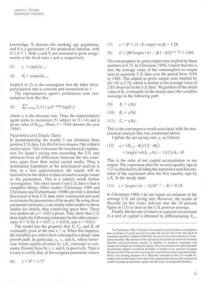
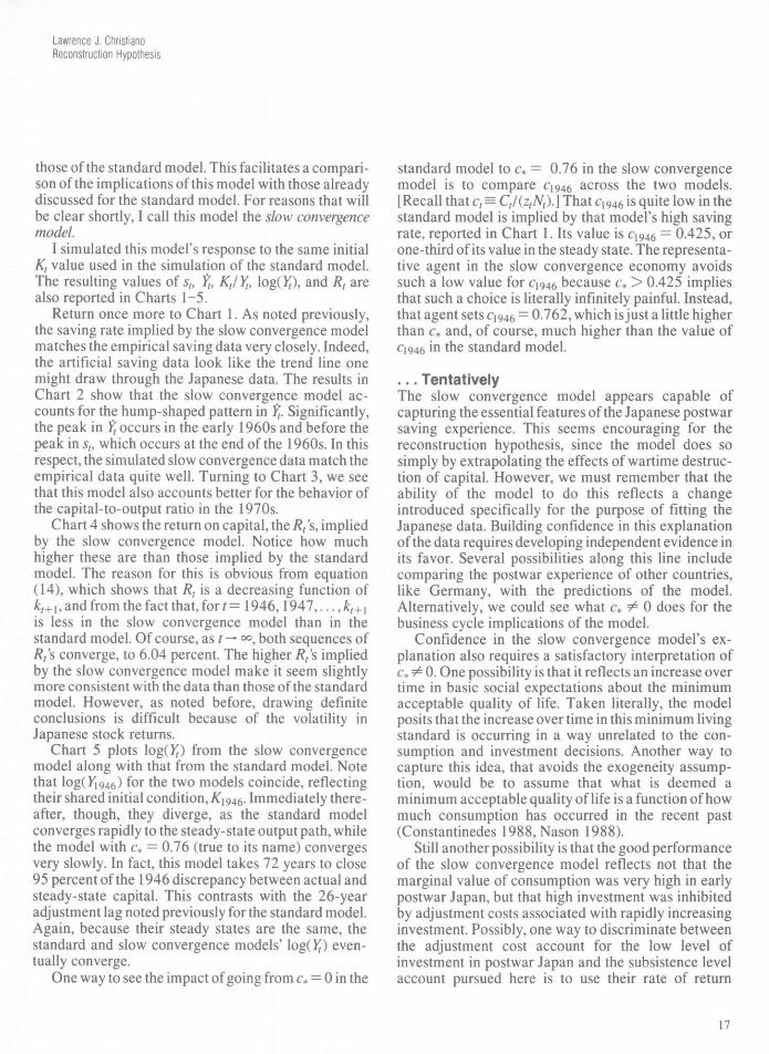
Turn first to Chart 1. The simulated graph of the saving rate, st, is the line marked standard model Note that the saving rate for this model peaks immediately at around 46 percent of NNP and then falls monotoni-cally. By 1972,26 years after 1946, the model has very nearly converged to its steady-state growth path. By

that year, for example, 95 percent of the 1946 discrep-ancy between actual and steady-state capital has been eliminated. Note how different the actual data are. They are hump-shaped and peak in 1970, at roughly the same time that the standard model has converged. (The actual data are from Hayashi's Chart 2 in this issue.)

Chart 2 graphs the growth in GNP, The standard model's pattern of % very much resembles that of st: % peaks immediately and then declines monotonically. This pattern also differs sharply from the actual data, which more or less display a hump shape.

The capital-to-output ratio is plotted in Chart 3. Note how quickly the standard model's ratio rises. Essentially, it has already converged to its steady-state value by the early 1970s, just when the corresponding actual values are rising most steeply. Note the U shape of the data: the capital-to-output ratio starts out rela-tively high in the mid-1950s, then falls, levels off, and rises. As noted above, the downward-sloping part of the U here is incompatible with the reconstruction hypoth-esis, in the context of the class of neoclassical growth models considered here. Thus, taking the reconstruction hypothesis seriously depends heavily on the validity of Hayashi's conjecture that the Japanese capital-to-output ratio in the 1950s is mismeasured. (The actual data here are from Hayashi's Chart 4 in this issue.)

The standard model's implied time path for the return on capital, Rt, is plotted in Chart 4. This return is predicted to be very high—31 percent—in 1946, but then it declines rapidly to its steady-state value of 6.04 percent. The erratic curve in Chart 4 is the inflation-adjusted return in the Japanese stock market, which I use as a crude indicator of the return to capital.6 The variance in that data series seems so large that it is very hard to say with confidence whether or not the Rt

9s implied by the standard model are consistent with the evidence. The model's /?,'s do, though, look a bit lower than the actual data.

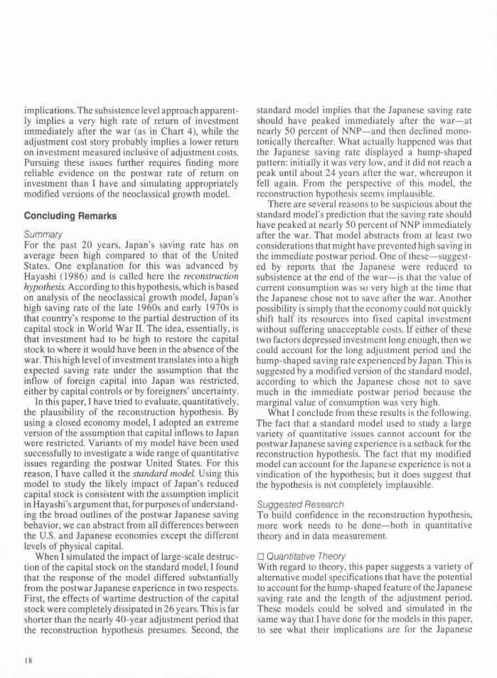
The path of log(^) is reported in Chart 5 to help give perspective on the results. The straight line is the steady-state output path that would by hypothesis have occurred had there been no destruction of Japanese capital. Note how quickly the standard model's log(}J) rises at first. This reflects the high initial values of shown in Chart 2.7

6Value-weighted nominal return data are from Japan 1988. Nominal returns are adjusted using the price deflator for personal consumption expendi-tures from the last quarter of the previous year to the last quarter of the current year, from Japan 1989a,b.

7 Output data are from Japan, various years.

1 4


Charts 1 - 4

The Reconstruction Hypothesis vs. The Japanese Data Predictions of Two Neoclassical Growth Models vs. Data for Various Japanese Economic Indicators

Chart 1 The Saving Rate (Annual Net Saving as a % of NNP, 1005/)

5 0

4 0

3 0

20

10

0 1 9 4 6 1 9 5 0 1960 1970

\ Standard \ Model

Actual \ Data

Slow - \ Convergence -

Model

I I 1 i i i i 1980 1990 1999

Chart 2 The Growth Rate (Annual % Change in GNP, 100)?)

%

2 5

20

1 5

10

5

0 - 5 1 9 4 6 1 9 5 0 1960 1970 1980 1990 1999

t Standard \ Model

-

\ K Actual - \ A A f l D a t a

- " H Slow Convergence

i | Model | | 1 1 1

Ratio 3.0

Chart 3 The Capital-to-Output Ratio (Kt/Yt)

2.5

2.0

1.5

1.0

.5

oianaara M o d e l , ^

T / A c t u a l J y° Data L ^ Slow Convergence Model

I I I i i l 1

Chart 4 The Return on Capital (/?,)

1 9 4 6 1 9 5 0 1960 1970 1980 1990 1999 1 9 4 6 1 9 5 0 1960 1970 1980 1990 1999

Chart 5

Shocked vs. Steady-State Output Output Predictions of Two Neoclassical Growth Models With and Without Destruction of Capital

Log (Yt) 2.5

Slow Convergence Model With Shock

Standard Model With Shock

,5 b L_ _L J_ 1 9 4 6 1 9 5 0 1960 1970 1980 1990 1999

Sources of actual data: Hayashi (in this issue), Japan Securities Research Institute, Japan Economic Planning Agency

15

. . . Significantly Several studies provide examples in which apparently large perturbations in decision rules actually have a small welfare impact in growth models like the stan-dard one considered here (Mirrlees and Stern 1972, Cochrane 1988, Smith 1989). In general, these exam-ples suggest the disconcerting possibility that tiny un-modeled costs—like computational costs and adjust-ment costs—that are associated with the optimal rule but not the perturbed rule could drastically affect model solutions. In the present context, if there were a small welfare difference between the optimal rule in the standard model and the actual historical decisions, then we would suspect the existence of very small, plausible changes in assumptions in the standard model that could reconcile it with the empirical evidence. Then we would be inclined to conclude that the differences between the standard model's predictions and the data are not economically significant. In fact, I find that the differences are extremely large economically.

A problem that has to be confronted in computing the welfare difference between the standard model's optimal rule and the data is that reliable data on Japanese consumption covering the first decade of the postwar period are not available. These are required for the welfare calculations. Therefore, instead of compar-ing the standard model's solution directly with the data, I compare it with the solution implied by a modified version of that model. The details of this model, which I call the slow convergence model, are described below. This model generates saving data that are essentially a smoothed version of the actual data (as is clear in Chart 1). For this reason, it seems reasonable to use this model's response to wartime destruction of physical capital as a proxy for the actual Japanese data.

The value to the standard model's representative agent of following the slow convergence plan given kx 946 = 0.12k = 0.5 87 is - 0 . 9 6 1 ? This plan is, of course, suboptimal in the context of the standard model. The value of behaving optimally in that model, given ^1946 — 0.054, is —0.9639 Thus, behaving optimally given an initial capital stock of 0.054 generates roughly the same amount of utility to the standard model's agent as does following the slow convergence policy and starting with capital of 0.587. This means that the standard model's representative agent who starts with

946 = 0.5 8 7 and is constrained to follow the sub-optimal policy would be willing to pay up to 90 percent of the capital stock in exchange for the privilege of following the optimal policy.10 This 90 percent figure seems quite large, which suggests that the difference

between the monotonically declining saving rate opti-mal in the standard model and the hump-shaped saving rate observed in the data is economically very large.

Modified, It Succeeds . . . The results examined in the charts so far indicate that the standard model cannot account for the main features of the postwar Japanese saving experience. Another look at Chart 1 suggests an obvious problem with that model. It predicts that Japan invests almost half of its NNP immediately after the war. There are at least two reasons why this might not have been desir-able. One is that shifting that many resources into investment might have generated unacceptable adjust-ment costs. Another is that the marginal value of current consumption might simply have been too high due to the population being very near subsistence.11

Either of these factors, which are not in the standard model, might have prevented the high level of invest-ment anticipated by that model.

To get a feel for the potential of these considerations to account for the Japanese experience, I replace the representative agent's preferences by these:

( 1 6 ) s r = i 9 4 6 [ l / ( l + p ) F 1 9 4 6 l o g ( Q - C*ZtNt)

for c* = 0.76. With these preferences, as Ct declines to its subsistence level, c*ztNt, the marginal utility of con-sumption shoots off to infinity, which discourages investment. A technical virtue of this parameterization is that its steady-state characteristics coincide with

8This was computed by substituting C/ for t = 1, 2, 3 , . . . , 900 into (5), where Ct

s is the optimal level of consumption implied by the slow convergence model.

9These numbers are an automatic by-product of the method I use to solve the model, which is described in detail in the Appendix. The value of fc1946 (that is, 0.054) associated with a welfare level of—0.963 is fairly precisely estimated since nearby values of&1946 generate very different welfare levels. In particular, given the values of fc1946 of 0.051, 0.054, and 0.056, the associated welfare levels are —1.013, —0.963, and —0.915, respectively.

10The welfare difference discussed here is a stock concept. There is also a flow concept. One such concept measures by what constant fraction consump-tion in the optimal plan has to be decreased for the resulting consumption sequence to generate the same utility as the suboptimal plan. The optimal plan in the standard model is worth 2.49, starting with &1946 = 0.587. The facts that the suboptimal plan is worth —0.963 in the standard model and that p = 0.03 imply that this constant fraction is 10 percent. This means that the representa-tive agent would be willing to pay up to 10 percent of consumption in the optimal plan indefinitely in exchange for being permitted to switch from the suboptimal to the optimal plan.

n F o r example, according to Jones (1985, p. 3), "Saving rates were low after the war, as real income was reduced to a near subsistence level." Jones apparently does not have a biological notion of subsistence in mind, since Japanese per capita income was higher in 1946 than it was in the first two decades of this century. (See Romer 1986, Fig. 1.)

16


those of the standard model. This facilitates a compari-son of the implications of this model with those already discussed for the standard model. For reasons that will be clear shortly, I call this model the slow convergence model

I simulated this model's response to the same initial Kt value used in the simulation of the standard model. The resulting values of st, % Kt/Yt, log(IJ), and Rt are also reported in Charts 1-5.

Return once more to Chart 1. As noted previously, the saving rate implied by the slow convergence model matches the empirical saving data very closely. Indeed, the artificial saving data look like the trend line one might draw through the Japanese data. The results in Chart 2 show that the slow convergence model ac-counts for the hump-shaped pattern in % Significantly, the peak in ^occurs in the early 1960s and before the peak in st, which occurs at the end of the 1960s. In this respect, the simulated slow convergence data match the empirical data quite well. Turning to Chart 3, we see that this model also accounts better for the behavior of the capital-to-output ratio in the 1970s.

Chart 4 shows the return on capital, the Rt\s, implied by the slow convergence model. Notice how much higher these are than those implied by the standard model. The reason for this is obvious from equation (14), which shows that Rt is a decreasing function of kt+x, and from the fact that, for t= 1946,1947, . . . , kt+l is less in the slow convergence model than in the standard model. Of course, as t —•* both sequences of Rt's converge, to 6.04 percent. The higher R/s implied by the slow convergence model make it seem slightly more consistent with the data than those of the standard model. However, as noted before, drawing definite conclusions is difficult because of the volatility in Japanese stock returns.

Chart 5 plots \og(Yt) from the slow convergence model along with that from the standard model. Note that log(r1946) for the two models coincide, reflecting their shared initial condition, K\946. Immediately there-after, though, they diverge, as the standard model converges rapidly to the steady-state output path, while the model with c* = 0.76 (true to its name) converges very slowly. In fact, this model takes 72 years to close 95 percent of the 1946 discrepancy between actual and steady-state capital. This contrasts with the 26-year adjustment lag noted previously for the standard model. Again, because their steady states are the same, the standard and slow convergence models' log(^) even-tually converge.

One way to see the impact of going from c* = 0 in the

standard model to c* = 0.76 in the slow convergence model is to compare c1946 across the two models. [Recall that ct= Ct/(ztNt).] That c1946 is quite low in the standard model is implied by that model's high saving rate, reported in Chart 1. Its value is c1946 = 0.425, or one-third of its value in the steady state. The representa-tive agent in the slow convergence economy avoids such a low value for c1946 because c* > 0.425 implies that such a choice is literally infinitely painful. Instead, that agent sets c1946 = 0.7 62, which is just a little higher than c* and, of course, much higher than the value of c1946 in the standard model.

. . . Tentatively The slow convergence model appears capable of capturing the essential features of the Japanese postwar saving experience. This seems encouraging for the reconstruction hypothesis, since the model does so simply by extrapolating the effects of wartime destruc-tion of capital. However, we must remember that the ability of the model to do this reflects a change introduced specifically for the purpose of fitting the Japanese data. Building confidence in this explanation of the data requires developing independent evidence in its favor. Several possibilities along this line include comparing the postwar experience of other countries, like Germany, with the predictions of the model. Alternatively, we could see what c* # 0 does for the business cycle implications of the model.

Confidence in the slow convergence model's ex-planation also requires a satisfactory interpretation of c* 0. One possibility is that it reflects an increase over time in basic social expectations about the minimum acceptable quality of life. Taken literally, the model posits that the increase over time in this minimum living standard is occurring in a way unrelated to the con-sumption and investment decisions. Another way to capture this idea, that avoids the exogeneity assump-tion, would be to assume that what is deemed a minimum acceptable quality of life is a function of how much consumption has occurred in the recent past (Constantinedes 1988,Nason 1988).

Still another possibility is that the good performance of the slow convergence model reflects not that the marginal value of consumption was very high in early postwar Japan, but that high investment was inhibited by adjustment costs associated with rapidly increasing investment. Possibly, one way to discriminate between the adjustment cost account for the low level of investment in postwar Japan and the subsistence level account pursued here is to use their rate of return

17

implications. The subsistence level approach apparent-ly implies a very high rate of return of investment immediately after the war (as in Chart 4), while the adjustment cost story probably implies a lower return on investment measured inclusive of adjustment costs. Pursuing these issues further requires finding more reliable evidence on the postwar rate of return on investment than I have and simulating appropriately modified versions of the neoclassical growth model.

Concluding Remarks

Summary For the past 20 years, Japan's saving rate has on average been high compared to that of the United States. One explanation for this was advanced by Hayashi (1986) and is called here the reconstruction hypothesis. According to this hypothesis, which is based on analysis of the neoclassical growth model, Japan's high saving rate of the late 1960s and early 1970s is that country's response to the partial destruction of its capital stock in World War II. The idea, essentially, is that investment had to be high to restore the capital stock to where it would have been in the absence of the war. This high level of investment translates into a high expected saving rate under the assumption that the inflow of foreign capital into Japan was restricted, either by capital controls or by foreigners' uncertainty.

In this paper, I have tried to evaluate, quantitatively, the plausibility of the reconstruction hypothesis. By using a closed economy model, I adopted an extreme version of the assumption that capital inflows to Japan were restricted. Variants of my model have been used successfully to investigate a wide range of quantitative issues regarding the postwar United States. For this reason, I have called it the standard model Using this model to study the likely impact of Japan's reduced capital stock is consistent with the assumption implicit in Hayashi's argument that, for purposes of understand-ing the broad outlines of the postwar Japanese saving behavior, we can abstract from all differences between the U.S. and Japanese economies except the different levels of physical capital.

When I simulated the impact of large-scale destruc-tion of the capital stock on the standard model, I found that the response of the model differed substantially from the postwar Japanese experience in two respects. First, the effects of wartime destruction of the capital stock were completely dissipated in 26 years. This is far shorter than the nearly 40-year adjustment period that the reconstruction hypothesis presumes. Second, the

standard model implies that the Japanese saving rate should have peaked immediately after the war—at nearly 50 percent of NNP—and then declined mono-tonically thereafter. What actually happened was that the Japanese saving rate displayed a hump-shaped pattern: initially it was very low, and it did not reach a peak until about 24 years after the war, whereupon it fell again. From the perspective of this model, the reconstruction hypothesis seems implausible.

There are several reasons to be suspicious about the standard model's prediction that the saving rate should have peaked at nearly 50 percent of NNP immediately after the war. That model abstracts from at least two considerations that might have prevented high saving in the immediate postwar period. One of these—suggest-ed by reports that the Japanese were reduced to subsistence at the end of the war—is that the value of current consumption was so very high at the time that the Japanese chose not to save after the war. Another possibility is simply that the economy could not quickly shift half its resources into fixed capital investment without suffering unacceptable costs. If either of these two factors depressed investment long enough, then we could account for the long adjustment period and the hump-shaped saving rate experienced by Japan. This is suggested by a modified version of the standard model, according to which the Japanese chose not to save much in the immediate postwar period because the marginal value of consumption was very high.

What I conclude from these results is the following. The fact that a standard model used to study a large variety of quantitative issues cannot account for the postwar Japanese saving experience is a setback for the reconstruction hypothesis. The fact that my modified model can account for the Japanese experience is not a vindication of the hypothesis; but it does suggest that the hypothesis is not completely implausible.

Suggested Research To build confidence in the reconstruction hypothesis, more work needs to be done—both in quantitative theory and in data measurement.

• Quantitative Theory With regard to theory, this paper suggests a variety of alternative model specifications that have the potential to account for the hump-shaped feature of the Japanese saving rate and the length of the adjustment period. These models could be solved and simulated in the same way that I have done for the models in this paper, to see what their implications are for the Japanese

18


saving rate and also for other variables, such as the return on investment and output growth.

Besides the quantitative theoretical exercises pro-posed above, it would be wise to simulate versions of the models in which hours worked can vary. Such a model—by implying that work effort in the immediate postwar period is unusually intense—would likely have a harder time accounting for the length of the adjust-ment lag. In addition, it would be of interest to study the impact of introducing international trade considera-tions into the neoclassical growth model. Presumably, permitting international capital flows would also in-crease the difficulty of accounting for the length of the adjustment lag using the reconstruction hypothesis.

Finally, it would be worthwhile to investigate the importance of the basic assumption of the neoclassical growth model, which is that the rate of progress of technological knowledge (zt/zt-{) is exogenous. More plausible is the assumption that this rate is endogenous and is affected by such things as investments in research and education. One expects that if something causes a jump in the return to investment in physical capital—as I have assumed happened in Japan—then resources will be transferred from sectors devoted to enhancing technical progress to sectors producing physical capital. The effect of this would be to reduce the pace of technical progress for a while, with the consequence that the economy's steady-state growth path is reduced. (This happens, essentially, because the parameter x is reduced for a while.) Thus, within a version of the neoclassical model, modified to make the pace of tech-nical progress endogenous, the reconstruction hypothe-sis is that U.S. output per capita remains permanently above Japanese output per capita, so that convergence never occurs. If these considerations are quantitatively important, then the fact that convergence between Japan and the United States seems to have occurred is an embarrassment for the reconstruction hypothesis.

With good quality data, quantitative exercises such as these would suggest which, if any, version of the reconstruction hypothesis provides a plausible account for the Japanese postwar experience.

• Data Measurement More good quality data are needed, too. Most impor-tant, we need to confirm Hayashi's suspicion (in this issue) that the high and falling Japanese capital-to-output ratio in the 1950s reflects measurement error. If it turns out to be wrong, then the reconstruction hypoth-esis has been dealt a major blow.

In addition, I have analyzed the reconstruction hy-

pothesis without any hard economic data for the first 10 years after the war. The only information I have is anecdotal evidence which suggests that saving was very low in this period. Besides data on the saving rate and other variables, reliable data on the rate of return on investment would be particularly informative. Rate of return movements are a key feature of the reconstruc-tion hypothesis, since high rates of return are what motivates the reconstruction phase. Also, I have argued that rate of return data can be used to discriminate between alternative versions of the neoclassical growth model that are being used to rationalize the reconstruc-tion hypothesis.

Research on other empirical issues would be useful as well. For example, my calculations have assumed that Japan started the postwar period 88 percent below its steady-state growth path for physical capital. More careful measurement of this is needed, since my esti-mate is based on sketchy data and is likely to be an overstatement. If so, then reconciling the reconstruction hypothesis with the nearly 40-year adjustment lag may be harder.

19

Appendix Solving a Neoclassical Growth Model

In the preceding paper, before I computed any model's responses to destruction of part of the capital stock, I had to first find the model's solution. By a solution, I mean a function relating current decisions about consumption and other vari-ables to variables that are currently fixed, such as the stock of physical capital, which maximize the utility function subject to the constraints. In this Appendix, I describe the method I used to find the solution to the two versions of the neoclassical growth model in the paper and how I used the solution to get the results reported there.

The solution to the model studied in the paper is not known, so that some sort of approximation is required. (For a summary of several existing methods, see Taylor and Uhlig 1989.) The easiest such approximation method is the linear quadratic (LQ) procedure proposed by Kydland and Prescott (1982). That method has been successfully applied in a business cycle context where the range of variation in the data is small enough that the method is very accurate. (On this, see Christiano 1989a.) However, in the application of this paper, the LQ solution may not be so accurate because the paper is concerned with the dynamic properties of a growth model under an extremely wide range of capital stock values. Solv-ing the model by a grid approximation method is, therefore, safer. Although this method is computationally costly, it can be tuned to generate as much accuracy as desired.

One thing most solution procedures have in common is the requirement that the variables in the model remain within some bounded set. That is obviously not a property of the model in this paper, since all the variables grow indefinitely. However, the variables are rendered stationary after division by ztNt. This is the basis of the transformation described below which converts the model into an alternative, equivalent model with variables that do remain in a bounded set. After that I give a precise mathematical statement of the objects computed using the model, followed by a description of the grid approximation method used to get them. Finally, I discuss how I went about tuning the grid approximation method to get an acceptable level of accuracy.

The Detrended Growth Model According to the model, a representative agent chooses con-sumption, C„ for t = 0, 1, 2, . . . to maximize the paper's equation (5) or (16) subject to equations (1M4) . 1 Define the detrended consumption and capital variables, ct and kt, as

( A l ) ct = CJ (ztNt)

(A2) kt = KJ (ztNt).

Expressed in terms of these variables, the agent's problem is to choose [c„ kt+l; t—0, 1, 2 , . . . } to maximize

(A3) K + o P log(c, - c.)

for p = 1/(1 +p ) subject to

(A4) ct + exp { x + n ) k t + x - (1 ~8)kt = ket.

For obvious reasons, I call this the detrended optimization problem. When c* = 0, this is the standard model, while c» = 0.76 defines the slow convergence model. In (A3), K = Xt=o ft \og(ztNt). Since this is simply an exogenous constant, it has no impact on the optimum and so is ignored from now on.

Substantively, whether the agent solves the original or the detrended optimization problem does not matter. This is because the choice variables in the former, C, and K ( + l , and those in the latter, ct and kt+h are related by a simple trans-formation. I introduce the detrended version of the problem only because the standard tools of mathematical optimization theory apply to it: In the original problem, Ct and Kt+l grow indefinitely; but in the detrended problem, ct and kt+x settle down to constant values as t —

The Properties of the Model Here I give a mathematical statement of the properties of the model that were of interest in the paper.

First, although I have posed the agent's problem as though it involves two choice variables, ct and kt+l, the resource constraint implies there is really only one choice. The problem is reduced to choosing kt+l by eliminating ct in (A3) using the constraint, (A4). Once that is done, the problem becomes to maximize, with respect to {kt+l; t = 0 ,1 ,2 , . . . } , 2 , = 0 P log[fc, -I- (1—d)k t — exp( jc+r i )k t + l — c J . This problem can be formulated as a dynamic programming problem:

( A 5 ) v(k) = mdixk'tA(k) {u(k,k') + / 3 v ( k ' ) }

where A(k) is the set of nonnegative k' for which the implied level of consumption, c, is nonnegative. Formally:

lrTo simplify the notation in the Appendix, I let t = 0 correspond to the year 1946, t = 1 to 1947, and so on.

2 0


( A 6 ) A(k) = {kf : 0 < k f < e x p ( - j t - n ) [kd + (1 - 8 ) k ] } .

Here, I follow the dynamic programming convention of dropping the t subscript. The variable k denotes the detrended physical stock of capital available at the beginning of the current period, and k' denotes the corresponding quantity available at the beginning of the next period. (Do not confuse the definition of k used here with the different one that appears in the paper.) In (A5),

(A7) u(k,k') = log[k d + ( 1 - 5 ) * - exp(j t+n)k ' - c j .

The problem is solved by first finding a value function, v, that satisfies (A5). Given v, the solution to the maximization prob-lem to the right of the equality in (A5) is a function (a decision rule) relating k! to k\ call it f(k). Given an initial value of k—say, A:0—this rule lets me compute a sequence kt =f(kt-{) for t = 1 ,2 ,3 , Given values for N0 and z0 ,1 can then get a sequence Kt for t = 1, 2, 3 , . . . using the kt*s, (Al) , and (A2). (I set N0 = z0= 1.) Given these K,'s, a sequence C, for t = 0 ,1 , 2 , . . . can be computed using (1). In addition, gross output, Yt, can be obtained from (2) for t = 0 ,1 ,2 , A sequence for the net saving rate, st for t — 0 , 1 , 2 , . . . , can be obtained from (12), and the /?/s can be computed using (14). The time paths of these variables are the model properties that are discussed in the paper.

The Grid Approximation Procedure The hard part in the calculations just described is the first step, finding the v function. Apart from a single special case, in which 8 = 1 and c* = 0, there is no known way of finding it, although v is known to exist. Still, though we don't know how to compute v exactly, we do have various ways to approxi-mate it. Each involves replacing the actual problem, (A5), with another problem which has a tractable solution that we hope is close to the solution of the actual problem.

The approximation procedure that seems most appro-priate here is the following. I assume that k can only take on a finite set of M values belonging to the grid k = {£,, k2, • • •,kM}. Her e f o r / = 1 , . . . ,M— 1. Thus, at any given time, the agent inherits some kek from the past and k! must be chosen from the intersection of A(k) and k. Formally, this is the problem:

( A 8 ) V(k) = matron* {w(U') + j8 V(k')}

for k e k . Let the decision rule that solves (A8) be denoted k' = F(k). The dependence of V and Fon the details of the grid, k, is suppressed to conserve notation. Solving (A8), in the sense of finding Vand F, is computationally tractable. More-over, F a n d / s h o u l d be virtually identical when Mis large and the grid, k, is fine.

I used the following iterative procedure to solve (A8). I set V°(k) = u(k,kx) for kek and then computed V1, V 2 , . . . , VJ as follows:

( A 9 ) VJ+Kk) = maxk,tMk)n~k {u(k,k') + fiVKk')}

fory = 0 , 1 , 2 , . . . , J— 1 and for all kek. For each j , I computed

(A10) rjj = max** |[VK& ~ Vj~\k)]IVKk)\ 100

where |- | denotes the absolute value. The integer J is defined as the first value of j for which r j j < 0.1~6.1 set V = VJ. The maximization in (A9) was done by evaluating the expression in braces at k! = k and at successively higher points in the k grid. The maximizing value of k! was assumed to be the point in k just before the first grid point where the value of the expression in braces falls. This method assumes that the expression in braces is concave in k\ a property known to be satisfied by the expression in braces in (A5).2

Now I need only describe exactly how I chose the grid, k. I know that my problem has exactly two steady-state values of k. [A steady-state value of k is defined by the property k =/(&).] Let k* and k* denote the smaller and larger of these, respectively. I set k{ = k* + 0.005 and kM = k*. Here, k* is the lowest nonnegative capital stock that lets c = c* be sustained indefinitely; that is, c* = + [ 1 — 8 — exp ( x + n ) ] k * . Obvi-ously, K — 0 when c* = 0. This bad steady state is unstable. The stable steady-state capital stock is k*. From (8):

( A l l ) k* = {fid/[exp(x+n) - /3(l-<5)]}1/(1-0).

The fact that k* (and, hence, c) is independent of c* reflects the constancy of the marginal utility of consumption in a steady state. As a result, the marginal utility of consumption does not appear in the steady-state intertemporal substitution in con-sumption. The reason for not considering values of k greater than k* is that I am only interested in the economy's response to a low initial value of k.

I experimented with two ways of selecting the intervals between kt and ki+l for i = 1 , . . . , M — 1 and with several settings for M. In one type of grid, the fixed interval grid, I let ki+l — kt be a constant for i = 1 , . . . , M — 1. In the other type of grid, the proportional interval grid, I let log(£ I+1 ) — log(£,) be a constant for i = I , . . . f M — 1. In this second grid type, the interval between kt and ki+l is roughly proportional to kt.

The Choice of a Capital Grid Now I describe the computational experiments used to decide on a grid type and a value for M.

Obviously, the appropriate grid type and value of M are those that produce an F function as similar as possible to the object of interest,/. This would be simple i f / w e r e available. Since it is not, I must instead base my choice of grid on indirect evidence about the similarity be tween/and F. I used two such pieces of evidence. Each focuses on the basic objective that motivates the calculations: to compute Rt, Yt, ?t, st, Kt/Yt for t = 0, 1 , 2 , . . . , 69 starting from k0 = 0A2k* and N0 = z0 = 1.

2More sophisticated versions of the grid approximation method are de-scribed in Bertsekas 1976. See also Christiano 1989a and Christiano and Fitzgerald 1989.

2 1

Tables A1 and A2

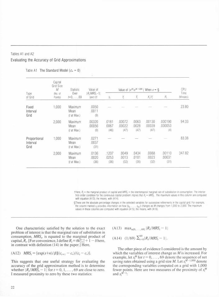
Evaluating the Accuracy of Grid Approximations

Table A1 The S tandard Mode l (c. = 0)

Capital Grid Size

M Statistic Value ot Value of \xM/xM''m | When x - § CPU Type (No. of Over \R,/MRSrM Time of Grid Points) t=0.....69 (andOt s, Yt K,/Yt R, (Minutes)

Fixed Interval Grid

Propor t iona l In terval Grid

1,000

2,000

1,000

2,000

Maximum .0050 — — — — —

Mean .0011 (t at Max.) (9)

Maximum .00320 .0181 .00072 .0063 .00130 .000190 Mean .00056 .0067 .00022 .0028 .00039 .000053 (t at Max.) (0) (46) (47) (47) (47) (4)

Maximum .0271 — —

Mean .0037 (/ at Max.) (31)

Maximum .0136 .1207 .0049 .0434 .0088 .00110 Mean .0020 .0253 .0013 .0101 .0023 .00031 (t at Max.) (36) (36) (32) (36) (32) (31)

23.80

94.33

83.38

347.82

tHere, R, = the marginal product of capital and MRS, = the intertemporal marginal rate of substitution in consumption. The interior first-order condition for the continuous capital problem implies that R, = MRS,. The maximum values in this column are computed with equation (A13); the means, with (A14).

§These are the absolute percentage changes in the selected variables for successive refinements in the capital grid. For example, the column marked s, provides information on how {SQ Sgg} changes as M changes from 1,000 to 2,000. The maximum values in these columns are computed with equation (A15); the means, with (A16).

One characteristic satisfied by the solution to the exact problem of interest is that the marginal rate of substitution in consumption, MRSt, is equated to the marginal product of capital, Rt. [For convenience, I define Rt = Oke,+\ + 1 — 6 here, in contrast with definition (14) in the paper.] Here,

(A 12) MRS, = [exp(jc+/i)/0][(c,+1 - c.)/(c, - c,)].

This suggests that one useful strategy for evaluating the accuracy of the grid approximation method is to determine whether | RJMRSt — 11 for t = O, 1 , . . . , 69 are close to zero. I measured proximity to zero by these two statistics:

(A 13) max,e{0 .., 69j \RtlMRSt — 11

(A 14) ( 1 / 6 9 ) 2 ^ 1 Rt/MRSt-l\.

The other piece of evidence I considered is the amount by which the variables of interest change as M is increased. For example, let s f for t = 0 , . . . , 69 denote the sequence of net saving rates obtained using a grid size M. Let stM~1'000 denote the corresponding variables computed on a grid with 1,000 fewer points. Here are two measures of the proximity of stM

and stM~l:

2 2


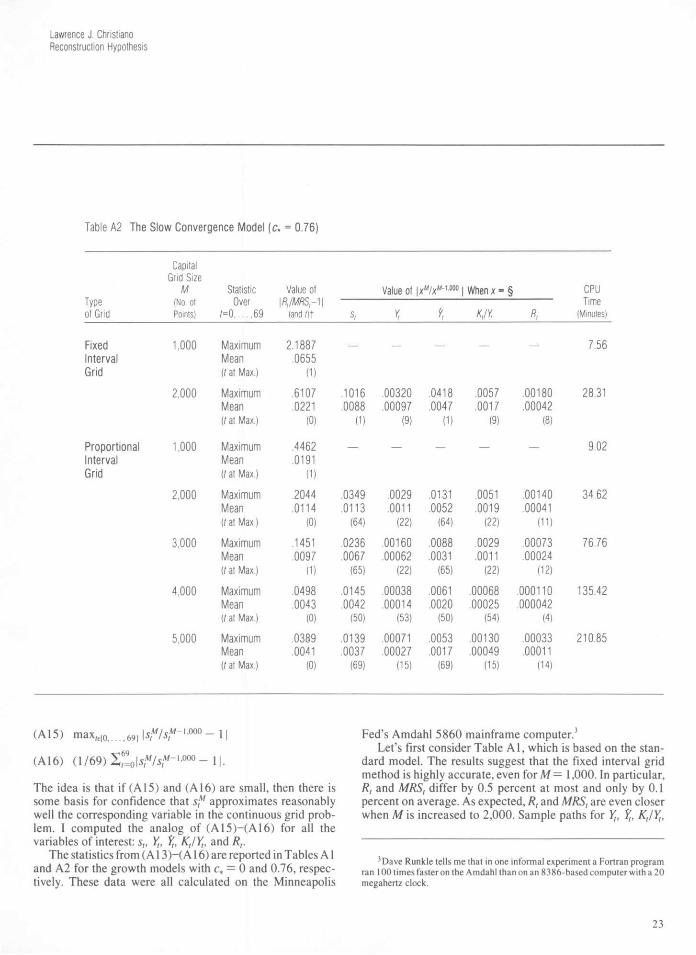
Table A2 The S low Conve rgence Mode l (c* = 0 .76 )

Capital Grid Size

M Statistic Value ot Value of \xM/xM~)m | When x = § CPU Type (No. of Over |/?,/M?S r1| Time of Grid Points) / = 0 , . . . , 6 9 (andOt s, Yt ?t K,/Y, R, (Minutes)

Fixed 1,000 Maximum 2.1887 In terva l Mean .0655 Grid (/at Max.) (1)

2 ,000 Maximum .6107 Mean .0221 (/at Max.) (0)

P ropor t i ona l 1,000 Maximum .4462 In terva l Mean .0191 Grid (/at Max.) (1)

2 ,000 Maximum .2044 Mean .0114 (/ at Max.) (0)

3 ,000 Maximum .1451 Mean .0097 (/at Max.) (1)

4 ,000 Maximum .0498 Mean .0043 (/ at Max.) (0)

5,000 Maximum .0389 Mean .0041 (/ at Max.) (0)

— — — — — 7.56

.1016

.0088 (1)

.00320

.00097 (9)

.0418

.0047 (1)

.0057

.0017 (9)

.00180

.00042 (8)

28.31

9.02

.0349

.0113 (64)

.0029

.0011 (22)

.0131

.0052 (64)

.0051

.0019 (22)

.00140

.00041 (11)

34.62

.0236

.0067 (65)

.00160

.00062 (22)

.0088

.0031 (65)

.0029

.0011 (22)

.00073

.00024 (12)

76.76

.0145

.0042 (50)

.00038

.00014 (53)

.0061

.0020 (50)

.00068

.00025 (54)

.000110

.000042 (4)

135.42

.0139

.0037 (69)

.00071

.00027 (15)

.0053

.0017 (69)

.00130

.00049 (15)

.00033

.00011 (14)

210 .85

(A 15) m a x r e { o , . . . , 6 9 } l W - 1 ' 0 0 0 - H

(A 16) (1/69) IstM/st

M~1 '00° — 11.

The idea is that if (A 15) and (A 16) are small, then there is some basis for confidence that st

M approximates reasonably well the corresponding variable in the continuous grid prob-lem. I computed the analog of (A15)-(A16) for all the variables of interest: st, Yt, ?t, Kt/Yt1 and Rt.

The statistics from (A 13)-(A 16) are reported in Tables A1 and A2 for the growth models with c* = 0 and 0.76, respec-tively. These data were all calculated on the Minneapolis

Fed's Amdahl 5860 mainframe computer.3

Let's first consider Table Al , which is based on the stan-dard model. The results suggest that the fixed interval grid method is highly accurate, even for M = 1,000. In particular, Rt and MRSt differ by 0.5 percent at most and only by 0.1 percent on average. As expected, Rt and MRSt are even closer when M is increased to 2,000. Sample paths for Yt, ?t, KJYV

3 Dave Runkle tells me that in one informal experiment a Fortran program ran 100 times faster on the Amdahl than on an 83 86-based computer with a 20 megahertz clock.

23

and Rt seem to have converged at M = 1,000, since the changes in these when M = 2,000 is very tiny. For example, the average change in fjis only about 0.3 percent. The change in st is somewhat greater—1.8 percent at most and 0.67 percent on average.

Table A1 also displays data for the proportional interval grid for comparison. The results primarily suggest that the proportional grid is slightly less accurate than the fixed grid. For example, Rt differs from MRS, an average of 0.2 percent when M = 2,000 and the grid is proportional, while the difference averages roughly 0.06 percent for that M when the grid is fixed. Therefore, the calculations in the paper for the model with c* = 0 are based on M = 2,000 and the fixed interval grid. Moreover, the evidence in this table gives us considerable confidence in the accuracy of the solution.

Now consider Table A2, which reports results based on the slow convergence model, with c* = 0.76. Note that here, with a fixed interval grid, when M = 1,000, R, is quite different from MRS„ indicating a potentially serious problem with the grid solution for this model. In particular, Rt differs from MRSt by as much as 219 percent for t— 1 and by roughly 7 percent on average. The situation improves for M= 2,000, though not by much compared to the results in Table A1. For example, R, still differs from MRSt by as much as 61 percent for t = 1 and by about 2 percent on average.

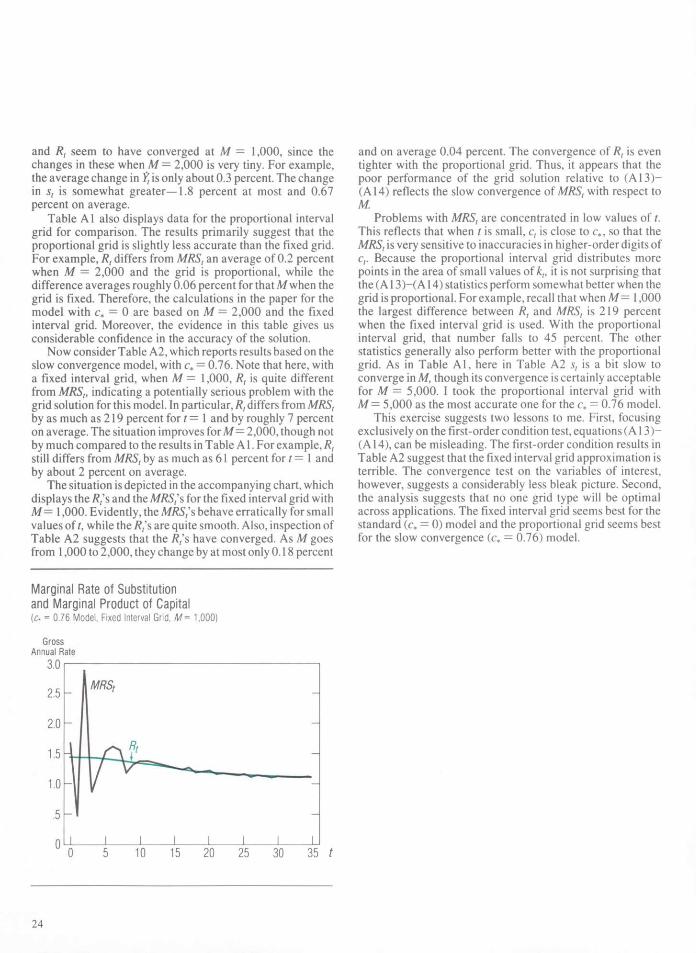
The situation is depicted in the accompanying chart, which displays the R, s and the MRS, s for the fixed interval grid with M= 1,000. Evidently, the MRS/s behave erratically for small values of t, while the /?/s are quite smooth. Also, inspection of Table A2 suggests that the Rt*s have converged. As M goes from 1,000 to 2,000, they change by at most only 0.18 percent

Marginal Rate of Substitution and Marginal Product of Capital [c* = 0 7 6 Model, Fixed Interval Grid, M= 1,000)

and on average 0.04 percent. The convergence of Rt is even tighter with the proportional grid. Thus, it appears that the poor performance of the grid solution relative to (A 13)-(A14) reflects the slow convergence of MRSt with respect to M.

Problems with MRS, are concentrated in low values of t. This reflects that when t is small, c, is close to c*, so that the MRSt is very sensitive to inaccuracies in higher-order digits of ct. Because the proportional interval grid distributes more points in the area of small values of kt, it is not surprising that the (A 13)-(A 14) statistics perform somewhat better when the grid is proportional. For example, recall that when M = 1,000 the largest difference between Rt and MRSt is 219 percent when the fixed interval grid is used. With the proportional interval grid, that number falls to 45 percent. The other statistics generally also perform better with the proportional grid. As in Table Al , here in Table A2 st is a bit slow to converge in M, though its convergence is certainly acceptable for M = 5,000. I took the proportional interval grid with M— 5,000 as the most accurate one for the c* = 0.76 model.

This exercise suggests two lessons to me. First, focusing exclusively on the first-order condition test, equations (A 13)-(A14), can be misleading. The first-order condition results in Table A2 suggest that the fixed interval grid approximation is terrible. The convergence test on the variables of interest, however, suggests a considerably less bleak picture. Second, the analysis suggests that no one grid type will be optimal across applications. The fixed interval grid seems best for the standard (c* = 0) model and the proportional grid seems best for the slow convergence (<:* = 0.76) model.

Gross Annual F

3 .0

2.5

2.0

1.5

1.0

.5

0

2 4


References

Barro, Robert J. 1987. Macroeconomics. 2nd ed. New York: Wiley. Bertsekas, Dimitri P. 1976. Dynamic programming and stochastic control. New

York: Academic Press. Braun, R. Anton. 1988. The dynamic interaction of distortionary taxes and aggre-

gate variables in postwar U.S. data. Manuscript. Northwestern University. Christiano, Lawrence J. 1987. Why is consumption less volatile than income?

Federal Reserve Bank of Minneapolis Quarterly Review 11 (Fall): 2-20. 1988. Why does inventory investment fluctuate so much 1 Journal

of Monetary Economics 21 (March/May): 247-80. 1989a. Solving a particular growth model by linear quadratic

approximation and by value function iteration. Discussion Paper 9. Institute for Empirical Macroeconomics (Federal Reserve Bank of Minneapolis and University of Minnesota).

1989b. Comments on "Consumption, income, and interest rates: Reinterpreting the time series evidence" by John Y. Campbell and N. Gregory Mankiw. Manuscript. Federal Reserve Bank of Minneapolis. Forthcoming in NBER Macroeconomics Annual 1989, ed. Olivier Blanchard. Cambridge, Mass.: MIT Press/National Bureau of Economic Research.

Christiano, Lawrence J., and Eichenbaum, Martin. 1988a. Human capital, endogenous growth and aggregate fluctuations. Manuscript. Federal Reserve Bank of Minneapolis.

1988b. Is theory really ahead of measurement? Current real business cycle theories and aggregate labor market fluctuations. Work-ing Paper 2700. National Bureau of Economic Research.

Christiano, Lawrence J., and Fitzgerald, Terry J. 1989. The magnitude of the speculative motive for holding inventories in a real business cycle model. Discussion Paper 10. Institute for Empirical Macroeconomics (Federal Reserve Bank of Minneapolis and University of Minnesota).

Cochrane, John H. 1988. The sensitivity of tests of the intertemporal allocation of consumption to near rational alternatives. Manuscript. University of Chicago.

Constantinedes, George M. 1988. Habit formation: A resolution of the equity premium puzzle. Manuscript. University of Chicago.

Hansen, Gary D. 1985. Indivisible labor and the business cycle. Journal of Monetary Economics 16 (November): 309-27.

Hayashi, Fumio. 1986. Why is Japan's saving rate so apparently high? In NBER Macroeconomics Annual 1986, ed. Stanley Fischer, pp. 147-210. Cambridge, Mass.: MIT Press/National Bureau of Economic Research.

Hodrick, Robert J.; Kocherlakota, Narayana; and Lucas, Deborah. 1988. The variability of velocity in cash-in-advance models. Manuscript. North-western University.

Japan. 1988. Rates of return on common stocks '87. Japan Securities Research Institute.

1989a. Annual report on national accounts, 1989. Economic Planning Agency, Government of Japan.

1989b. Report on national accounts from 1955 to 1969. Econom-ic Planning Agency, Government of Japan.

Various years. Annual report on national accounts. Economic Planning Agency, Government of Japan.

Jones, Randy. 1985. Report. Japan Economic Institute (1000 Connecticut Avenue, NW, Washington, D.C. 20036).

Kydland, Finn E., and Prescott, Edward C. 1982. Time to build and aggregate fluctuations. Econometrica 50 (November): 1345-70.

Mirrlees, J. A., and Stern, N. H. 1972. Fairly good plans. Journal of Economic Theory 4 (April): 268-88.

Nason, James M. 1988. The equity premium and time-varying risk behavior. Finance and Economics Discussion Series 11. Board of Governors of the Federal Reserve System.

Prescott, Edward C. 1986. Theory ahead of business cycle measurement. Federal Reserve Bank of Minneapolis Quarterly Review 10 (Fall): 9-22. Also in Real business cycles, real exchange rates and actual policies, ed. Karl Brunner and Allan H. Meltzer. Carnegie-Rochester Conference Series on Public Policy 25 (Autumn): 11-44. Amsterdam: North-Holland.

Romer, Paul M. 1986. Comment on "Why is Japan's saving rate so apparently high?" by Fumio Hayashi. In NBER Macroeconomics Annual 1986, ed. Stanley Fischer, pp. 220-33. Cambridge, Mass.: MIT Press/National Bureau of Economic Research.

Smith, Anthony. 1989. Solving nonlinear rational expectations models: A new approach. Manuscript. Duke University.

Solow, Robert M. 1956. A contribution to the theory of economic growth. Quarterly Journal of Economics 70 (February): 65-94.

Taylor, John B., and Uhlig, Harald. 1989. Solving nonlinear stochastic growth models: A comparison of alternative solution methods. Manuscript. Stanford University.

U.S. President. 1989. Economic report of the President. Washington, D.C.: U.S. Government Printing Office.

25

high? (p 3.) - connecting repositories · high? (p 3.) fumio hayashi understanding japan's...

Documents