195

GIScience & Remote Sensing, 2011, 48, No. 2, p. 195–209. DOI: 10.2747/1548-1603.48.2.195Copyright © 2011 by Bellwether Publishing, Ltd. All rights reserved.

Herbaceous Biomass Estimation from SPOT 5 Imagery in Semiarid Rangelands of Idaho

Fang Chen,1 Keith T. Weber, and Bhushan Gokhale GIS Training and Research Center, Idaho State University, 921 S. 8th Ave, Stop 8104, Pocatello Idaho 83209-8104

Abstract: Eight vegetation indices (VI) commonly used for above-ground biomass (AGB) estimation were derived from Satellite Pour l’Observation de la Terre 5 (SPOT 5) imagery and used to predict herbaceous AGB at a semiarid rangeland study site in southeastern Idaho. The relationship between herbaceous AGB and vegetation water content was also evaluated and as a result, a suite of water-sensitive vegetation indi-ces (WSVI) were developed. Correlation coefficients between herbaceous AGB, VIs, and WSVIs were calculated, demonstrating that WSVIs were correlated (r2 ≥ 0.51) with vegetation water content and performed better than standard VIs in herbaceous AGB estimates within the semiarid rangelands of Idaho.

INTRODUCTION

Rangelands cover approximately 40% of the earth’s terrestrial surface and are important areas for livestock production and wildlife habitat (Breman and de Wit, 1983; Huntsinger and Hopkinson, 1996). To effectively manage rangelands it is impor-tant to assess ecosystem productivity and biomass production (Running et al., 2004). Biomass estimates represent the quantity of matter in a given area and are expressed either as the weight of organisms per unit area or as the volume of organisms per unit volume. Previous total above-ground biomass (AGB) research has demonstrated that vegetation indices (VI) are sensitive to the biophysical and biochemical variations in vegetation, and as a result are the most common parameters used to estimate AGB (Davidson and Csillag, 2001; Kawamura et al., 2005; Numata et al., 2008). A remote sensing–derived VI is a quantitative optical measure of canopy greenness (Tucker, 1979; Weiser et al., 1986). Various VIs, such as the normalized difference vegetation index (NDVI), normalized difference water index (NDWI), and soil adjusted veg-etation index (SAVI), have been correlated with AGB, and applied to predict AGB within a variety of biomes (Davidson and Csillag, 2001; Kogan et al., 2004; Mirik et al., 2005; Wessels et al., 2006; Numata et al., 2008; Cho and Skidmore, 2009) (Table 1). Recently, ground-based and satellite-based spectral measurement methods have been developed to better quantify AGB. For instance, many ground-based methods use portable field spectroradiometers or digital cameras (e.g., ASD spectrometers, ASD Inc., Boulder, CO, USA; Dycam Agricultural Digital Camera (ADC), Dycam Inc., Chatworth, CA, USA) to collect canopy radiance and predict AGB through an

1Corresponding author; email: chenfang@isu.edu

196 chen et al.

empirical relationship between spectral values and biomass samples (Boelman et al., 2003; Flynn et al., 2008; Mašková et al., 2008). These methods are straightforward and accurate for small-area studies (e.g., approximately 1–10 ha); however, they are also labor intensive and difficult to apply over broad spatial scales or long-term tem-poral scales.

The increasing availability of satellite-based remote sensing data extends the assessment of AGB to a broader spatiotemporal scale. For example, remotely sensed data acquired from various sensors have been used to assess AGB, including NOAA’s AVHRR (Box et al., 1989; Sannier et al., 2002; Kogan et al., 2004; Wessels et al., 2006), MODIS (Kawamura et al., 2005; Xu et al., 2008), Landsat-5 TM and Landsat-7 ETM+ (Friedl et al., 1994; Schino et al., 2003; Samimi and Kraus, 2004), SPOT VEGETATION (Verbesselt et al., 2006b), and hyperspectral sensors such as PROBE-1, Hyperion, and the HyMap system (Mutanga and Skidmore, 2004; Mirik et al., 2005; Numata et al., 2008; Cho and Skidmore, 2009).

Although many studies have investigated the ability to assess AGB from VIs, many problems have been found. One problem is that an empirical relationship derived

Table 1. Correlation of Vegetation Indices with Total Above-Ground Biomass (AGB) Reported in Different Studies

Study area Sensor Index R2 Sources

Kentucky, USA Greenseeker RT500

NDVI 0.68 Flynn et al., 2008

Southern Africa Landsat7 -ETM+ Green/blue 0.85 Samimi and Kraus, 2004

Inner Mongolia, China

MODIS NDVI 0.75 Kawamura et al., 2005

Italy HyMap NDVI 0.32–0.58 Cho and Skidmore, 2009NDWI 0.49–0.55

Czech Republic ADC NDVI 0.83(managed)

Mašková et al., 2008

0.52(unmanaged)

Namibia AVHRR NDVI 0.76 Sannier et al., 2002

Northern Alaska

UniSpec-DC NDVI 0.84 Boelman et al., 2003

Italy NDVI 0.32 Schino et al., 2003

Brazilian Amazon

Analytical Spectral Device

NDVI 0.03 Numata et al., 2008

NDWI 0.13

herbaceous biomass estimation 197

by a VI for the accurate prediction of AGB at one site or time period may not apply to other sites or even the same site at another time (Foody et al., 2003). This problem is primarily due to variations in the natural environment (e.g., variable precipitation, soil-water content, and temperature conditions), viewing season (e.g., phenology dur-ing the growing season), and the sensor used in the study (e.g., differences in spatial resolution and other sensor characteristics) (Davidson and Csillag, 2001; Schino et al., 2003; Flynn et al., 2008). In addition, because VIs have differing abilities to provide accurate estimates of AGB, it is difficult to determine an optimal VI for a specific study. For example, the same VI (e.g., NDVI) may have different prediction accuracies within various regions, yet different types of VIs (e.g., NDVI vs NDWI) may perform quite differently within the same region (Table 1). These problems limit the transfer-ability of predictive relationships and the effectiveness of VIs to estimate AGB.

Approximately 48% of Idaho is considered rangeland, and many of these areas are categorized as a semiarid sagebrush-steppe ecosystem (http://www.idrange.org). AGB estimation in the semiarid rangelands of the Intermountain West plays an impor-tant role in rangeland ecosystem assessment. In the semiarid rangelands of Idaho, high temperatures hasten the desiccation of plants, and many grass species senesce during the summer. The relationship between herbaceous AGB and VIs is most accu-rately estimated when the proportion of green or growing material is high (Hill, 2004; Numata et al., 2008) relative to the proportion of bare ground and/or litter. While important, determining an optimal VI for the accurate estimation of seasonal herba-ceous AGB in semiarid rangelands may be difficult.

Most VIs used for AGB estimation are based on radiance or reflectance from a red band (RED) around 0.66 µm and a near infrared band (NIR) around 0.86 µm (Huete et al., 2002; Chuvieco et al., 2004). The RED band characteristically shows a strong chlorophyll absorption region for vegetation and strong reflectance for soils, while the NIR band is located in the high reflectance plateau of vegetation canopies. Because absorption by liquid water near 0.86 µm is negligible, NIR reflectance is affected primarily by internal leaf structure and cellulose content (Gao, 1996). In contrast, the short-wave infrared band (SWIR) (around 1.24 µm) is located in the high reflec-tance plateau of vegetation reflectance with weak liquid absorption (canopy scattering enhances the water absorption) (Jacquemoud et al., 1996; Jackson et al., 2004). The SWIR band reflects changes in both the vegetation water content and the spongy mes-ophyll structure of vegetation. The combination of the NIR band with the SWIR band can remove variation induced by internal leaf structure and leaf dry matter content (Gao, 1996; Ceccato et al., 2001). This combination of these bands (NIR and SWIR) is also sensitive to changes in liquid water content within the vegetation canopy (Serrano et al., 2000; Zarco-Tejada et al., 2003).

In this study, a suite of water-sensitive vegetation indices (WSVI) were devel-oped, incorporating the NIR and SWIR portions of the electromagnetic spectrum, to help characterize plant water content and better estimate herbaceous AGB in semiarid rangeland ecosystems. The study was designed to investigate the applicability of vari-ous VIs for the assessment of herbaceous AGB in the semiarid rangelands of Idaho, USA. To accomplish this, eight VIs—including the difference vegetation index (DVI; Richardson and Everitt, 1992), ratio vegetation index (RVI; Jordan, 1969), normal-ized difference vegetation index (NDVI; Rouse et al., 1973), re-normalized difference vegetation index (RDVI; Roujean and Breon, 1995), soil adjusted vegetation index

198 chen et al.

(SAVI; Huete 1988), the second modified soil adjusted vegetation index (MSAVI2; Qi et al. 1994), infrared percentage vegetation index (IPVI; Crippen, 1990), and modified simple ratio (MSR; Chen, 1996)—were derived from Satellite Pour l’Observation de la Terre 5 (SPOT 5) imagery. In addition, the relationship between herbaceous AGB and total water content was determined. Finally, correlation estimates between her-baceous AGB, VIs, and WSVIs were calculated, and the performance of herbaceous AGB predictions from both VIs and WSVIs were evaluated using field-based mea-surements of herbaceous AGB.

MATERIALS AND METHODS

Study Area

The study area, known as the Big Desert, lies in southeastern Idaho, USA, approx-imately 71 km northwest of Pocatello. The center of the study area was located at 113° 4’ 18.68” W and 43° 14’ 27.88” N (Fig. 1). This area is managed by the U.S. Bureau of Land Management (BLM) and exhibits a large variety of native as well as invasive plant species. The area is a semiarid sagebrush-steppe ecosystem with a high propor-tion of bare ground ( x bare ground > 17%; Studley et al., 2009). The area is sagebrush steppe, consisting primarily of native and non-native grasses, forbs, and many shrub species, including sagebrush (Artemisia tridentata) and rabbit brush (Chrysothamnus nauseosus). Annual precipitation is 23 cm, with 40% of the precipitation falling from April through June. The area is bordered by geologically young lava formations to the south and west and irrigated agricultural lands to the north and east. Sheep grazing is the primary anthropogenic disturbance to the study area, with semi-extensive continu-ous/seasonal grazing systems used on allotments ranging in size from 1100 to over 125,000 ha. Wildfire is a common disturbance and nearly 40% of the study area has burned in the past 10 years.

Field Data Collection

This study presents results using total herbaceous AGB measurements only, and does not include any measurements of shrub biomass production. Twenty-nine sample locations were selected for the collection of herbaceous AGB, which has been defined for the purposes of this study as all grasses, forbs, and standing litter. Site selection criteria included the site being a homogeneous area at least 20 m × 20 m in size (cf., spatial resolution of SPOT satellite imagery = 10 m × 10 m in size, thus helping to assure the sample pixel was also homogeneous), with still larger areas being preferred. The dominant plants in each site are herbaceous vegetation, with the plot center > 70 m from any “edges,” including roads, fences, or power lines, and plot perimeters >100 m from all other plots. Preference was given to sites with perimeters located >250 m apart. The location of each sample plot center was recorded using a Trimble Geo XH GPS receiver using latitude-longitude (WGS 84). All GPS data were post-process differentially corrected (±0.10 m after post-processing with a 95% CI using reference stations located <80 km from the study area) to ensure the sample location was registered with the correct and representative pixel within the satellite imagery (Weber, 2006; Weber et al., 2008).

herbaceous biomass estimation 199

Available herbaceous AGB was measured using a plastic-coated cable hoop 2.36 m in circumference. The hoop was randomly tossed into each of four quadrants (NW, NE, SE, and SW) centered over the sample point. All herbaceous vegetation within the hoop was clipped as close to the ground as allowed by the clipper (approximately 5 mm from the ground surface) and weighed immediately (±1 g) using a Pesola scale tared to the weight of an ordinary paper bag. The samples were taken to the laboratory, and dried in 75°C ovens for 48 hours. After drying, the samples were re-weighed to determine vegetation water content. Biomass was estimated following Sheley (1999) and expressed in kilograms per hectare.

Vegetation Indices Derived from SPOT 5-Imagery

Satellite Pour l’Observation de la Terre 5 (SPOT 5) multispectral imagery (10 m × 10 m pixels) was acquired for the Big Desert study area on June 27, 2009. The imagery was georectified against 2004 National Agriculture Imagery Program (NAIP) natural color aerial imagery (1 m ×1 m pixels). Atmospheric correction was performed with Idrisi Taiga (v16.03) using the ATMOSC module (Clark Labs, Worcester, MA). All imagery was corrected for atmospheric effects using the Cos(t) model (Chavez, 1996) and input parameters reported in the metadata supplied by SPOT Image Corporation. The imagery was then projected into Idaho Transverse Mercator (NAD 83). The eight VIs used in this study were derived from the SPOT 5 imagery.

Fig. 1. Location and general characteristics of the Big Desert in southeastern, Idaho. No weather station survey site was available within the Big Desert study area; however, nine sites were located that bound the study area. Although some sites are in the mountains, the weather there exhibits a similar trend compared to that of the Snake River Plain.

200 chen et al.

Water Sensitive Vegetation Indices

Using the same SPOT 5 imagery, eight WSVIs were developed by directly substi-tuting the SWIR band for the RED band within the eight VIs described above (Table 2). The “Sample” tool within ESRI’s ArcGIS 10 was then used to extract VI and WSVI values at each sample site (n = 29). The resulting data were exported to SPSS (V17.0) for further analysis. Correlations between VI/WSVI values and measured herbaceous AGB were used to determine the applicability and efficacy of each.

RESULTS AND DISCUSSION

Field-based herbaceous AGB estimates ranged from 518 kg/ha to 8075 kg/ha ( x = 2982 kg/ha) based on vegetation samples collected at 29 field locations. Using linear regression analysis between each VI and herbaceous AGB measurements, the relationship between these variables was described (Table 3). Based upon these results, it was noted that the relationships varied greatly and the strength of all cor-relations were relatively weak (0.28 ≤ r2 < 0.40). This was likely attributable to the mixture of photosynthetic and non-photosynthetic plant material found in the field, and correspondingly in the herbaceous AGB samples used in this study. As a result, the VIs provided poor estimates of herbaceous AGB. Furthermore, the prediction of

Table 2. Water-Sensitive Vegetation Indices Used to Estimate Herbaceous Total Above-Ground Biomassa

Index Formula

DWI NIR SWIR–

RWI NIR SWIR⁄

NDWI NIR SWIR–NIR SWIR+---------------------------------

RDWI NIR SWIR–

NIR SWIR+-------------------------------------

SAWI NIR SWIR–( ) 1 L+( )NIR SWIR L+ +

-------------------------------------------------------- where L 0.5=,

MSAWI2 2NIR 1 2NIR 1+( )2 8 NIR SWIR–( )––+2

----------------------------------------------------------------------------------------------------------------

IPWI NIRNIR SWIR+---------------------------------

MWSR

NIRSWIR---------------- 1–

NIRSWIR---------------- 1+

-----------------------------

aNote the substitution of the SWIR band for the RED band (cf. Table 3).

herbaceous biomass estimation 201

herbaceous AGB was least well explained using NDVI (r2 = 0.28, p = 0.003); as a result, NDVI was not considered a reliable predictor of herbaceous AGB in this study area, although it remains one of most widely used VIs for AGB prediction and many other vegetation studies.

Based on field survey data, the relationship between herbaceous AGB and veg-etation water content (Fig. 2) revealed a significant correlation (r2 = 0.94, p < 0.001). Related studies have shown that grass biophysical parameters such as leaf area index are related to liquid water content (Hunt and Rock, 1989; Roberts et al., 1997, 2004). Numata et al. (2008) indicated water absorption spectra between 1100 and 1250 nm had a significant correlation with canopy water content and suggested that the use of water absorption features (i.e., water absorption depth and water absorption area) may improve the accuracy of biomass estimation. Therefore, the hypothesis that an index

Table 3. Correlation between Herbaceous Total Above-Ground Biomass and the VIs and WSVIs Used in This Study

Standard VIs using RED and NIR bands Water-sensitive VIs using NIR and SWIR bandsIndex r2 F-value p Index r2 F-value p

DVI 0.40 17.9 <0.001 DWI 0.53 30.1 <0.001RVI 0.35 14.3 0.001 RWI 0.54 31.2 <0.001NDVI 0.28 10.6 0.003 NDWI 0.52 29.0 <0.001RDVI 0.35 14.3 0.001 RDWI 0.52 29.8 <0.001SAVI 0.37 15.8 <0.001 SAWI 0.53 29.8 <0.001MSAVI2 0.39 17.0 <0.001 MSAWI2 0.53 30.3 <0.001IPVI 0.28 10.6 0.003 IPWI 0.52 29.0 <0.001MSR 0.32 12.6 0.001 MWSR 0.53 30.3 <0.001

Fig. 2. Relationship between herbaceous total above-ground biomass (AGB) and vegetation water content.

202 chen et al.

that closely correlates to water content may also exhibit strong correlation with herba-ceous AGB was tested.

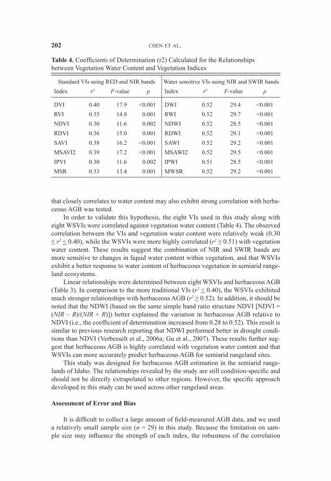
In order to validate this hypothesis, the eight VIs used in this study along with eight WSVIs were correlated against vegetation water content (Table 4). The observed correlation between the VIs and vegetation water content were relatively weak (0.30 ≤ r2 < 0.40), while the WSVIs were more highly correlated (r2 ≥ 0.51) with vegetation water content. These results suggest the combination of NIR and SWIR bands are more sensitive to changes in liquid water content within vegetation, and that WSVIs exhibit a better response to water content of herbaceous vegetation in semiarid range-land ecosystems.

Linear relationships were determined between eight WSVIs and herbaceous AGB (Table 3). In comparison to the more traditional VIs (r2 < 0.40), the WSVIs exhibited much stronger relationships with herbaceous AGB (r2 ≥ 0.52). In addition, it should be noted that the NDWI (based on the same simple band ratio structure NDVI [NDVI = (NIR – R)/(NIR + R)]) better explained the variation in herbaceous AGB relative to NDVI (i.e., the coefficient of determination increased from 0.28 to 0.52). This result is similar to previous research reporting that NDWI performed better in drought condi-tions than NDVI (Verbesselt et al., 2006a; Gu et al., 2007). These results further sug-gest that herbaceous AGB is highly correlated with vegetation water content and that WSVIs can more accurately predict herbaceous AGB for semiarid rangeland sites.

This study was designed for herbaceous AGB estimation in the semiarid range-lands of Idaho. The relationships revealed by the study are still condition-specific and should not be directly extrapolated to other regions. However, the specific approach developed in this study can be used across other rangeland areas.

Assessment of Error and Bias

It is difficult to collect a large amount of field-measured AGB data, and we used a relatively small sample size (n = 29) in this study. Because the limitation on sam-ple size may influence the strength of each index, the robustness of the correlation

Table 4. Coefficients of Determination (r2) Calculated for the Relationships between Vegetation Water Content and Vegetation Indices

Standard VIs using RED and NIR bands Water sensitive VIs using NIR and SWIR bandsIndex r2 F-value p Index r2 F-value p

DVI 0.40 17.9 <0.001 DWI 0.52 29.4 <0.001RVI 0.35 14.8 0.001 RWI 0.52 29.7 <0.001NDVI 0.30 11.6 0.002 NDWI 0.52 28.5 <0.001RDVI 0.36 15.0 0.001 RDWI 0.52 29.1 <0.001SAVI 0.38 16.2 <0.001 SAWI 0.52 29.2 <0.001MSAVI2 0.39 17.2 <0.001 MSAWI2 0.52 29.5 <0.001IPVI 0.30 11.6 0.002 IPWI 0.51 28.5 <0.001MSR 0.33 13.4 0.001 MWSR 0.52 29.2 <0.001

herbaceous biomass estimation 203

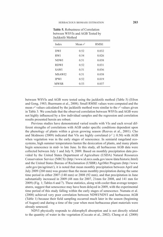
between WSVIs and AGB were tested using the jackknife method (Table 5) (Efron and Gong, 1983; Buermann et al., 2008). Small RMSE values were computed and the mean r2 values calculated by the jackknife method were similar to the r2 values given in Table 3. We conclude that the observed correlation between WSVIs and AGB were not highly influenced by a few individual samples and the regression and correlation results presented herein are robust.

Previous studies have demonstrated varied results with VIs and each reveal dif-ferent strengths of correlations with AGB under specific conditions dependent upon the phenology of plants within a given growing season (Reeves et al., 2001). Cho and Skidmore (2009) indicated that VIs are highly correlated (r2 ≥ 0.50) with AGB when vegetation was in the early stages of senescence. In semiarid rangeland eco-systems, high summer temperatures hasten the desiccation of plants, and many plants begin senescence in mid- to late June. In this study, all herbaceous AGB data were collected between July 1 and July 9, 2009. Based on monthly precipitation data pro-vided by the United States Department of Agriculture (USDA) Natural Resources Conservation Service (NRCS) (http://www.id.nrcs.usda.gov/snow/data/historic.html) and the United States Bureau of Reclamation (USBR) AgriMet Program (http://www .usbr.gov/pn/agrimet/), it is noted that mean monthly precipitation between April and July 2009 (260 mm) was greater than the mean monthly precipitation during the same time period in either 2007 (140 mm) or 2008 (92 mm), and that precipitation in June substantially increased in 2009 (48 mm for 2007, 21mm for 2008, and 141 mm for 2009) (Fig. 1; Tables 6 and 7). These statistics, along with cooler than average temper-atures, suggest that senescence may have been delayed in 2009, with the experimental time period of this study falling within the early stages of senescence. Numata et al. (2008) achieved very poor correlation between NDWI/NDVI and herbaceous AGB (Table 1) because their field sampling occurred much later in the season (beginning of August) and during a time of the year when most herbaceous plant materials were already senesced.

NDVI physically responds to chlorophyll absorption and is not directly related to the quantity of water in the vegetation (Ceccato et al., 2002). Cheng et al. (2008)

Table 5. Robustness of Correlation between WSVIs and AGB Tested by Jackknife Method

Index Mean r2 RMSE

DWI 0.52 0.032RWI 0.54 0.026NDWI 0.51 0.038RDWI 0.52 0.031SAWI 0.51 0.036MSAWI2 0.51 0.038IPWI 0.52 0.019MWSR 0.53 0.037

204 chen et al.Ta

ble

6. N

atur

al R

esou

rces

Con

serv

atio

n Se

rvic

e (N

RC

S) a

nd A

griM

et S

urve

y Si

te L

ist a

long

with

Mon

thly

Pre

cipi

tatio

n

and

Mon

thly

Mea

n Te

mpe

ratu

re

Site

nam

eLa

t.Lo

ng.

Year

Prec

ipita

tion,

mm

Mea

n te

mpe

ratu

re, °

C

Apr

ilM

ayJu

neJu

lyTo

tal

Apr

ilM

ayJu

ne

Gar

field

R.S

.43

°36′

–113

°55′

2007

438

2528

104

913

1920

0823

4313

2310

216

1920

2009

3071

203

2032

48

1016

Swed

e Pe

ak43

°37′

–113

°58′

2007

5615

3038

139

813

1920

0825

283

056

712

1820

0928

4320

123

295

79

15Sm

iley

Mou

ntai

n43

°43′

–113

°50′

2007

8933

8915

226

610

1720

0830

9448

1318

53

815

2009

8991

180

4340

35

713

How

ell C

anyo

n42

°19′

–113

°36′

2007

150

3011

725

322

812

1820

0856

7658

1520

55

1017

2009

124

6617

03

363

79

16W

ildho

rse

Div

ide

42°4

5′–1

12°2

8′20

0786

2574

1319

810

1318

2008

3666

330

135

712

1720

0910

758

163

3636

49

1116

Fort

Hal

l43

°04′

–112

°25′

2007

305

395

7913

1723

2008

337

94

5311

1620

2009

3129

9715

172

1215

20R

uper

t42

°35′

–113

°52′

2007

199

208

5614

1723

2008

317

127

3912

1721

2009

2618

536

103

1315

21Pi

cabo

43°1

8′–1

14°0

9′20

0723

310

339

1318

2420

087

227

036

1116

2120

0920

4198

816

712

1420

Abe

rdee

n42

°57′

–112

°49′

2007

363

3014

8314

1823

2008

423

61

3412

1621

2009

2322

102

1716

413

1520

herbaceous biomass estimation 205

indicate that NDVI’s correlation with water content was probably due to a correlation with green leaf density. Because of the sparse vegetation and dry plant matter (litter) found in semiarid regions, NDVI was not a reliable indicator of water content or her-baceous AGB in this study. However, some AGB estimates have shown strong NDVI correlations to biomass (r2 ≥ 0.50), but this may be because these study areas were more homogeneous and/or contained a higher proportion of green grass cover (Mašková et al. 2008). The accuracy of herbaceous AGB predictions based upon remotely sensed data is strongly influenced by the presence and abundance of grass species as well as the presence and abundance of bare ground and other spectral distraction features. A more homogeneous surface always provides higher correlations between remotely sensed measures and herbaceous AGB estimates compared to more heterogeneous surfaces (Numata et al., 2008). In addition, as opposed to the traditional VI, the WSVIs have the advantage of leveraging liquid water absorption regions to more accurately predict water content even in areas without contiguous spectral coverage (Serrano et al., 2000). This is possibly one reason why the WSVIs performed better in the semiarid rangelands of Idaho.

CONCLUSION

This study has focused on estimation of herbaceous AGB in the semiarid range-lands of Idaho. Based on a survey of herbaceous AGB, a significant correlation (p < 0.001) between herbaceous AGB and vegetation water content was found. In addition, a suite of WSVIs were developed that describe water content and herbaceous AGB in semiarid rangeland ecosystems. Correlation estimates between herbaceous AGB, VIs, and WSVIs were calculated, and the performance of herbaceous AGB predic-tions for both the VIs and WSVIs were evaluated using field-based measurements of herbaceous AGB. Results demonstrate that the WSVIs were correlated (r2 ≥ 0.51) with vegetation water content and performed better in herbaceous AGB estimation for the semiarid rangelands of Idaho relative to VIs. Furthermore, it was noticed that not only did vegetation water content influence the accuracy of herbaceous AGB estimates, but based on findings reported in other studies, phenological stage and plant commu-nity structure also influence the accuracy of herbaceous AGB estimates derived from remotely sensed data. Numerous factors influence the successful use of remote sensing data for the estimation of herbaceous AGB, and water content, described using WSVIs, explained approximately 50% of the variance in herbaceous AGB measurements

Table 7. Analysis of Precipitation and Temperature on 2007, 2008, and 2009

YearAverage precipitation, mm Average temperature, ° C Total

precipitationStandard deviation April May June July May June July

2007 59 15 48 17 11 15 20 140 56a

2008 20 45 21 7 9 14 19 92 69b

2009 53 49 141 19 10 12 17 260

aStandard deviation of precipitation for 2007 and 2008.bStandard deviation of precipitation for 2008 and 2009.

206 chen et al.

collected as part of this study. Other factors that likely play a role include sun angle, shadow, georegistration, and the varying affect of soils. Future work will seek to assess a more comprehensive characterization of the influence of these factors on herbaceous AGB estimations in semiarid rangelands.

ACKNOWLEDGMENTS

This study was made possible by a grant from the National Aeronautics and Space Administration Goddard Space Flight Center (NNX08AO90G). Idaho State University would also like to acknowledge the Idaho Delegation for their assistance in obtaining this grant.

REFERENCES

Boelman, N. T., Stieglitz, M., Rueth, H. M., Sommerkorn, M., Griffin, K. L., Shaver, G. R., and J. A. Gamon, 2003, “Response of NDVI, Biomass, and Ecosystem Gas Exchange to Long-term Warming and Fertilization in Wet Sedge Tundra,” Oecologia, 135(3):414–421.

Box, E. O., Holben, B. N., and V. Kalb, 1989, “Accuracy of the AVHRR Vegetation Index as a Predictor of Biomass, Primary Productivity, and Net CO2 Flux,” Plant Ecology, 80(2):71–89.

Breman, H., and C. T. de Wit, 1983, “Rangeland Productivity and Exploitation in the Sahel,” Science, 221(4618):1341–1347.

Buermann, W., Saatchi, S., Smith, T. B., Zutta, B. R., Chaves, J. A., Milá, B., and C. H. Graham, 2008, “Predicting Species Distributions Across the Amazonian and Andean Regions Using Remote Sensing Data,” Journal of Biogeography, 35(7):1160–1176.

Ceccato, P., Flasse, S., and J. M. Gregoire, 2002, “Designing a Spectral Index to Esti-mate Vegetation Water Content from Remote Sensing Data: Part 2. Validation and Applications,” Remote Sensing of Environment, 82(2–3):198–207.

Ceccato, P., Flasse, S., Tarantola, S., Jacquemond, S., and J. M. Gregoire, 2001, “Detecting Vegetation Leaf Water Content Using Reflectance in the Optical Domain,” Remote Sensing of Environment, 77(1):22–33.

Chavez, P. S., Jr, 1996, “Image-Based Atmospheric Corrections: Revisited and Improved,” Photogrammetric Engineering and Remote Sensing, 62(9):1025–1036.

Chen, J. M., 1996, “Evaluation of Vegetation Indices and a Modified Simple Ratio for Boreal Applications,” Canadian Journal of Remote Sensing, 22(3):229–242.

Cheng, Y. B., Ustin, S. L., Riaño, D., and V. C. Vanderbilt, 2008, “Water Content Estimation from Hyperspectral Images and MODIS Indexes in Southeastern Arizona,” Remote Sensing of Environment, 112(2):363–374.

Cho, M. A., and A. K. Skidmore, 2009, “Hyperspectral Predictors for Monitoring Biomass Production in Mediterranean Mountain Grasslands: Majella National Park, Italy,” International Journal of Remote Sensing, 30(2):499–515.

Chuvieco, E., Cocero, D., Riaño, D., Martin, P., Martínez-Vega, J., Riva, J. D. L., and F. Pérez, 2004, “Combining NDVI and Surface Temperature for the Estimation

herbaceous biomass estimation 207

of Live Fuels Moisture Content in Forest Fire Danger Rating,” Remote Sensing of Environment, 92(3):322–331.

Crippen, R. E., 1990, “Calculating the Vegetation Index Faster,” Remote Sensing of Environment, 34(1):71–73.

Davidson, A., and F. Csillag, 2001, “The Influence of Vegetation Index and Spatial Resolution on a Two-Date Remote Sensing–Derived Relation to C4 Species Coverage,” Remote Sensing of Environment, 75(1):138–151.

Efron, B., and G. Gong, 1983, “A Leisurely Look at the Bootstrap, the Jackknife, and Cross-validation,” American Statistician, 37(1):36–48.

Flynn, E. S., Dougherty, C. T., and O. Wendroth, 2008, “Assessment of Pasture Biomass with the Normalized Difference Vegetation Index from Active Ground-Based Sensors,” Agronomy Journal, 100(1):114–121.

Foody, G. M., Boyd, D. S., and M. E. J. Cutler, 2003, “Predictive Relations of Tropi-cal Forest Biomass from Landsat TM Data and Their Transferability between Regions,” Remote Sensing of Environment, 85(4):463–474.

Friedl, M. A., Michaelsen, J., Davis, F. W., Walker, H., and D. S. Schimel, 1994, “Estimating Grassland Biomass and Leaf Area Index Using Ground and Satellite Data,” International Journal of Remote Sensing, 15(7):1401–1420.

Gao, B. C, 1996, “NDWI: A Normalized Difference Water Index for Remote Sens-ing of Vegetation Liquid Water from Space,” Remote Sensing of Environment, 58(3):257–266.

Gu, Y., Brown, J. E., Verdin, J. P., and B. Wardlow, 2007, “A Five-Year Analysis of MODIS NDVI and NDWI for Grassland Drought Assessment over the Central Great Plains of the United States,” Geophysical Research Letters, 34(L06407) [doi: 10.1029/2006GL029127].

Hill, M. J., 2004, “Grazing Agriculture: Managed Pasture, Grassland, and Rangeland,” in Manual of Remote Sensing, Volume 4. Remote Sensing for Natural Resource Management and Environmental Monitoring, Ustin S. L.(Ed.). Hoboken, NJ: John Wiley & Sons, 449–530.

Huete, A. R., 1988, “A Soil-Adjusted Vegetation Index (SAVI),” Remote Sensing of Environment, 25(3):295–309.

Huete, A. R., Didan, K., Miura, T., Rodriguez, E. P., Gao, X., and L. G. Ferreira, 2002, “Overview of the Radiometric and Biophysical Performance of the MODIS Vegetation Indices,” Remote Sensing of Environment, 83(1–2):195–213.

Hunt, E. R. and B. N. Rock, 1989, “Detection of Changes in Leaf Water Content Using Near- and Middle-Infrared Reflectances,” Remote Sensing of Environment, 30(1):43–54.

Huntsinger, L. and P. Hopkinson, 1996, “Viewpoint: Sustaining Rangeland Land-scapes: A Social and Ecological Process,” Journal of Range Management, 49(2):167–173.

Jackson, T. J., Chen, D., Cosh, M., Li, F., Anderson, M., Walthall, C., Doriaswamy, P., and E. R. Hunt, 2004, “Vegetation Water Content Mapping Using Landsat Data–Derived Normalized Difference Water Index for Corn and Soybeans,” Remote Sensing of Environment, 92(4):475–482.

Jacquemoud, S., Ustin, S. L., Verdebout, J., Schmuck, G., Andreoli, G., and B. Hosgood, 1996, “Estimating Leaf Biochemistry Using the PROSPECT Leaf Optical Proper-ties Model,” Remote Sensing of Environment, 56(3):194–202.

208 chen et al.

Jordan, C. F., 1969, “Derivation of Leaf Area Index from Quality of Light on the For-est Floor,” Ecology, 50(4):663–666.

Kawamura, K., Akiyama, T., Yokota, H., Tsutsumi, M., Yasuda, T., Watanabe, O., and S. Wang, 2005, “Comparing MODIS Vegetation Indices with AVHRR NDVI for Monitoring the Forage Quantity and Quality in Inner Mongolia Grassland, China,” Grassland Science, 51(1):33–40.

Kogan, F., Stark, R., Gitelson, A., Jargalsaikhan, L., and S. Tsooj, 2004, “Derivation of Pasture Biomass in Mongolia from AVHRR-Based Vegetation Health Indices,” International Journal of Remote Sensing, 25(14):2889–2896.

Mašková, Z., Zemek, F., and J. Kvet, 2008, “Normalized Difference Vegetation Index (NDVI) in the Management of Mountain Meadows,” Boreal Environmental Research, 13(5):417–432.

Mirik, M., Norland, J., Crabtree, R., and M. Biondini, 2005, “Hyperspectral One-Meter-Resolution Remote Sensing in Yellowstone National Park, Wyoming: II. Biomass,” Rangeland Ecology and Management, 58(5):459–465.

Mutanga, O., and A. K. Skidmore, 2004, “Hyperspectral Band Depth Analysis for a Better Estimation of Grass Biomass (Cenchrus ciliaris) Measured under Con-trolled Laboratory Conditions,” International Journal of Applied Earth Observa-tion and Geoinformation, 5(2):87–96.

Numata, I., Roberts, D. A., Chadwick, O. A., Schimel, J. P., Galvão, L. S., and J. V. Soares, 2008, “Evaluation of Hyperspectral Data for Pasture Estimate in the Brazilian Amazon Using Field and Imaging Spectrometers,” Remote Sensing of Environment, 112(4):1569–1583.

Qi, J., Chehbouni, A, Huete, A. R., Kerr, Y. H., and S. Sorooshian, 1994, “A Modi-fied Soil Adjusted Vegetation Index,” Remote Sensing of Environment, 48(2):119–126.

Reeves, M. C., Winslow, J. C., and S. W. Running, 2001, “Mapping Weekly Range-land Vegetation Productivity Using MODIS Algorithms,” Rangeland Ecology & Management, 54:A90–A105.

Richardson, A. J., and J. H. Everitt, 1992, “Using Spectral Vegetation Indices to Esti-mate Rangeland Productivity,” Geocarto International, 7(1):63–69.

Roberts, D. A., Green, R. O., and J. B. Adams, 1997, “Temporal and Spatial Pat-terns in Vegetation and Atmospheric Properties from AVIRIS,” Remote Sensing of Environment, 62(3):223–240.

Roberts, D. A., Ustin, S. L., Ogunjemiyo, S., Greenberg, J., Dobrowski, S. Z., Chen, J. Q., and T. M. Hinckley, 2004, “Spectral and Structural Measures of Northwest Forest Vegetation at Leaf to Landscape Scales,” Ecosystems, 7(5):545–562.

Roujean, J. L., and F. M. Breon, 1995, “Estimating PAR Absorbed by Vegetation from Bidirectional Reflectance Measurements,” Remote Sensing of Environment, 51(3):375–384.

Rouse, J. W., Haas, R. H., Schell, J. A., and D. W. Deering, 1973, “Monitoring Vegeta-tion Systems in the Great Plains with ERTS,” in The 3rd Earth Resources Tech-nology Satellite Symposium, 10–14 December 1973, Washington, DC, 309–317.

Running, S. W., Nemani, R. R., Heinsch, F. A., Zhao, M., Reeves, M. C., and H. Hashimoto, 2004, “A Continuous Satellite-Derived Measure of Global Terrestrial Primary Production,” BioScience, 54(6):547–560.

herbaceous biomass estimation 209

Samimi, C., and T. Kraus, 2004, “Biomass Estimation Using Landsat-TM and -ETM+. Towards a Regional Model for Southern Africa?” GeoJournal, 59(3):177–187.

Sannier, C. A. D., Taylor, J. C., and W. Du Plessis, 2002, “Real-Time Monitoring of Vegetation Biomass with NOAA-AVHRR in Etosha National Park, Namibia, for Fire Risk Assessment,” International Journal of Remote Sensing, 23(1):71–89.

Schino, G., Borfecchia, F., Cecco, L., Dibari, C., Iannetta, M., Martini, S., and F. Pedrotti, 2003, “Satellite Estimate of Grass Biomass in a Mountainous Range in Central Italy,” Agroforestry Systems, 59(2):157–162.

Serrano, L., Ustin, S. L., Roberts, D. A., Gamon, J. A., and J. Peñuelas, 2000, “Deriv-ing Water Content of Chaparral Vegetation from AVIRIS Data,” Remote Sensing of Environment, 74(3):570–581.

Sheley, R. 1999, AUM Analyzer Software, Bozeman, MT: Montana State University [http://www.montana.edu], accessed March 31, 2010.

Studley, H. and K. T. Weber, 2009, “Range Vegetation Assessment in the Big Desert, Upper Snake River Plain, Idaho” [http://giscenter.isu.edu/research/Techpg/nasa_postfire/To_PDF/2009_Big Desert_FieldReport.pdf], accessed March 31, 2010.

Tucker, C. J., 1979, “Red and Photographic Infrared Linear Combinations for Moni-toring Vegetation,” Remote Sensing of Environment, 8(2):127–150.

Verbesselt, J., Jonsson, P., Lhermitte, S., van Aardt, J., and P. Coppin, 2006a, “Eval-uating Satellite and Climate Data–Derived Indices as Fire Risk Indicators in Savanna Ecosystems,” IEEE Transactions on Geoscience and Remote Sensing, 44(6):1622–1632.

Verbesselt, J., Somers, B., van Aardt, J., Jonckheere, I., and P. Coppin, 2006b, “Moni-toring Herbaceous Biomass and Water Content with SPOT VEGETATION Time-Series to Improve Fire Risk Assessment in Savanna Ecosystems,” Remote Sensing of Environment, 101(3):399–414.

Weber, K. T., 2006, “Challenges of Integrating Geospatial Technologies into Range-land Research and Management,” Rangeland Ecology and Management, 59(1):38–43.

Weber, K. T., Theau, J., and K. Serr, 2008, “Effect of Co-registration Error on Patchy Target Detection Using High-Resolution Imagery,” Remote Sensing of the Envi-ronment, 112(3):845–850.

Weiser, R. L., Asrar, G., Miller, G. P., and E. T. Kanemasu, 1986, “Assessing Grass-land Biophysical Characteristics from Spectral Measurements,” Remote Sensing of the Environment, 20(2):141–152.

Wessels, K. J., Prince, S. D., Zambatis, N., MacFadyen, S., Frost, P. E., and D. Van Zyl, 2006, “Relationship between Herbaceous Biomass and 1-km2 Advanced Very High Resolution Radiometer (AVHRR) NDVI in Kruger National Park, South Africa,” International Journal of Remote Sensing, 27(5):951–973.

Xu, B., Yang, X. C., Tao, W. G., Qin, Z. H., Liu, H. Q., Miao, J. M., and Y. Y. Bi, 2008, “MODIS-Based Remote Sensing Monitoring of Grass Production in China,” International Journal of Remote Sensing, 29(17):5313–5327.

Zarco-Tejada, P. J., Rueda, C. A., and S. L. Ustin, 2003, “Water Content Estimation in Vegetation with MODIS Reflectance Data and Model Inversion Methods,” Remote Sensing of Environment 85(1):109–124.