helicopter electromagnetic sea ice thickness estimation: an
TRANSCRIPT

Helicopter Electromagnetic sea ice thickness estimation: An induction method in the centimetre scale Meereisdickenbestimmung mittels Hubschrauber-elektromagnetik: Ein Induktionsverfahren im Zentimeterbereich
Andreas Pfaffling

Andreas Pfaffling
Alfred Wegener Institut für Polar- und Meeresforschung Postfach 120161 27515 Bremerhaven
Die vorliegende Arbeit ist die inhaltlich unveränderte Fassung einer kumulativen Doktorarbeit, die 2006 dem Fachgebiet Geowissenschaften der Universität Bremen vorgelegt wurde
I
CONTENT
Abstract II Zusammenfassung IV
List of Acronyms VI
THESIS 1 Introduction 3
Sea Ice and Climate Change...................................................................................... 3 Sensors & methods in sea ice research ...................................................................... 4 The need for a direct sea ice thickness measure......................................................... 7
Adapting Helicopter electromagnetics for sea ice 11 Advanced footprint definition ................................................................................. 11 System calibration & precision ............................................................................... 12 Sea ice conductivity, target or bias? ........................................................................ 13 Data quality versus inversion .................................................................................. 14 Outlook................................................................................................................... 14
Acknowledgments 16
References 17
Appendix 24 Publication List....................................................................................................... 24 High conductivies and the “Mundry-Integral”......................................................... 26 MATLAB® 1D forward model ................................................................................ 27 Bibliographic details of papers I-IV ........................................................................ 29
PAPER I 31 Reid, J.E., Pfaffling, A., and Vrbancich, J. 2006. Airborne electromagnetic footprints in 1D earths.
PAPER II 43 Pfaffling, A., Haas, C., and Reid, J.E. 2006. A direct helicopter EM sea ice thickness inversion, assessed with synthetic and field data.
PAPER III 67 Pfaffling, A., and Reid, J.E. 2006. Sea ice as an evaluation target for HEM modeling and inversion
PAPER IV 87 Reid, J.E., Pfaffling, A., Worby, A.P., and Bishop, J.R. 2006. In-situ measurements of the direct-current conductivity of Antarctic sea ice: implications for airborne electromagnetic sounding of sea ice thickness
II
ABSTRACT With Climate Change and Global Warming in the public debate, research is strongly
focusing on methods to gain information on changes in the Polar regions. Most of our knowledge about the effects and phenomena in the past, present and future is based on remote sensing and computer models. While there is various information available about sea ice concentration and extent, little is known about the evolution of sea ice thickness. All long term, regional sea ice thickness data available, depend on assumptions and approximations to indirectly estimate the desired thickness distribution. Helicopter electromagnetics (HEM) has become the accepted tool to calibrate and validate satellite ice thickness data as well as to conduct regional scale inter-annual sea ice thickness change investigations. Constituting the truth for remote sensing data, it is of ultimate importance to know about the precision and accuracy of HEM ice thickness estimates. This doctoral thesis focuses on those key values and their governing factors. The thesis is a methodical work revisiting some basic HEM algorithms and approximations as well as investigating the influence of calibration, sensitivity, noise, drift, a priori information, etc. emphasising on the effects on sea ice thickness retrieval.
With respect to technical noise and calibration quality, the desired HEM sea ice thickness precision of 10 cm can be met1. However, a challenging small noise level of less than 5 ppm is needed for this result. Pitch and roll of the airborne system is not accounted for, though identified as a further source for biased ice thickness. Investigations on the footprint size reveal different values for components measured. Typical footprint sizes are 2.7 times or 4.6 times the system altitude for the quadrature or in-phase component respectively. Consequently the lateral size of a profiled feature (e.g. sea ice pressure ridge) needs to be at least one footprint, so that the thickness can be retrieved correctly from one-dimensional (1D) data processing. As HEM sea ice data is 1D processed and pressure ridges are usually smaller than the footprint, the maximum ridge thickness is commonly underestimated by more than 50 %. In situ sea ice conductivity measurements in Antarctica confirm the strong vertical to horizontal anisotropy of sea ice. As only the small horizontal conductivity is picked up by the induction process, this has a strong impact on HEM sea ice thickness modelling. Sea ice conductivies usually assumed for modelling, have been too high.
A suite of several layered earth inversion algorithms applied on synthetic and field sea ice data yielded diverse results. Inverted thickness estimates are mostly comparable but not better than the otherwise used approximate EM data to ice thickness transform (look-up table). The desired sea ice conductivity can’t be extracted from inversion for thin ice up to 3 m and neither for conductive pressure ridge keels. The odd combination of system frequencies and ice + water conductivies appears to be the cause for the failure, rather than inversion in general. However, inversion is capable to account for highly conductive surface layers (gap layer, slush) and to estimate shallow water bathymetry under a thin Baltic sea ice cover. Both gap layer or shallow water would bias the look-up table thickness estimates.
1 Note that the given synopsis of findings is solely valid for the AWI - HEM system.

III
Besides improving the knowledge about HEM sea ice thickness accuracy, this thesis also comprises findings of interest for the general HEM community, such as the advanced footprint definition, the triad of precision – sensitivity – noise and considering sea ice as a validation target for geophysical instruments and methods.
IV
ZUSAMMENFASSUNG In Zeiten von Klimaänderung und Erderwärmung wird in der Forschung mehr und
mehr Wert auf die Erschließung von Informationen aus den Polargebieten gelegt. Der Großteil unseres Wissens über die Prozesse und Phänomene in der Vergangenheit, Gegenwart und Zukunft stammt aus Erkenntnissen der Fernerkundung und von Computersimulationen. Im Gegensatz zu der breiten Auswahl an verfügbaren Informationen zur Meereiskonzentration und –Ausdehnung, wissen wir wenig über die Entwicklung der Meereisdicke. Die verfügbaren großflächigen Langzeitmeereisdickendaten beruhen auf Annahmen und Vereinfachungen, die es erlauben die Dicke indirekt zu bestimmen. Hubschrauber Elektromagnetik (HEM) wird als Verfahren zur Kalibration und Validierung dieser Fernerkundungsdaten angesehen und für regionale, langfristige Studien herangezogen. Somit ist es von immenser Wichtigkeit, die Genauigkeit und Präzision der HEM Eisdicken zu kennen. Diese Doktorarbeit konzentriert sich auf diese Kennwerte und deren beeinflussende Faktoren. Es handelt sich um eine methodische Arbeit, die Grundlegende Verfahren und Vereinfachungen der HEM (wieder-)beurteilt, sowie die Einflussgrößen Kalibration, Sensitivität, Geräterauschen, Gerätedrift, a - priori Informationen, usw. untersucht, im Hinblick auf die Auswirkungen auf HEM Meereisdickenbestimmung.
Ausgehend von Geräterauschen und Kalibrierungsqualität kann für das AWI HEM System die gewünschte Meereisdicken-Messgenauigkeit von 10 cm erreicht werden. Allerdings muss ein vergleichsweise niedriges Geräterauchen von maximal 5 ppm erreicht werden. Nicken und Rollen des Systems gehen in die erwähnten Genauigkeitsbetrachtungen nicht ein, obwohl sie als weitere Ungenauigkeitsquelle aufgeführt werden. Eine Untersuchung der „Footprint“-größe zeigt unterschiedliche Ergebnisse für die beiden Komponenten des gemessenen elektromagnetischen Feldes. Typische Footprintgrößen sind 2.7 mal die Systemhöhe für den Imaginärteil bzw. 4.6 mal für den Realteil. Folglich muss die laterale Ausdehnung eines Objektes (z.B. Presseisrücken) mindestens die Größe des Footprints erreichen, um eine korrekte Dickenbestimmung zu gewährleisten, unter der Voraussetzung das Eindimensionale (1D) Auswerteverfahren im Einsatz sind. Da HEM Meereisdicken mittels 1D Verfahren gewonnen werden und Presseisrücken üblicherweise schmaler als der Footprint sind, wird deren maximale Dicke um mehr als 50 % unterschätzt. Die ausgeprägte Anisotropie (vertikal zu horizontal) von Meereis wird anhand von Leitfähigkeitsmessungen auf Antarktischem Meereis bestätigt. Da beim Induktionsvorgang nur die horizontale Leitfähigkeit eine Rolle spielt, hat die beschriebene Anisotropie eine fundierte Auswirkung auf HEM Meereisdickenmodellierung. Herkömmlicherweise angenommene Meereisleitfähigkeiten waren überhöht.
Mehrere verschiedene Inversionsverfahren, angewandt an synthetische HEM Daten und Messergebnisse liefern mannigfaltige Ergebnisse. Invertierte Meereisdicken sind generell vergleichbar aber nicht besser als die Ergebnisse des herkömmlichen, vereinfachten direkten Transformationsverfahrens. Die erhoffte Meereisleitfähigkeit kann durch Inversion nicht bestimmt werden, weder für relative dünnes Eis (< 3 m) noch für Presseisrückenkiele. Die Auslegung der zwei Systemfrequenzen in Kombination mit den kontrastierenden Leitfähigkeiten von Meerwasser und –eis, wird

V
als Ursache für den Misserfolg angeraten. Andererseits liefert Inversion erfolgreiche Meereisdicken für Meereisleitfähigkeitsanomalien (gap layer, slush) sowie seichte Wassertiefen für Ostseebedingungen. Sowohl gap layer als auch Untiefen unter Ostseeeis würden die direkte Transformation negativ beeinflussen.
Abgesehen vom Fortschritt im Wissen um HEM Meereisdicken-Messgenauigkeit, können in dieser Arbeit auch Ergebnisse gefunden werden, die von generellem geophysikalischen Interesse sind. Beispiele sind die erweiterte Footprint Beschreibung, die Dreiecksbeziehung Präzision – Sensitivität – Geräterauschen oder die generelle Wahrnehmung von Meereis als ein Validationsobjekt für geophysikalische Methoden und Geräte.
VI
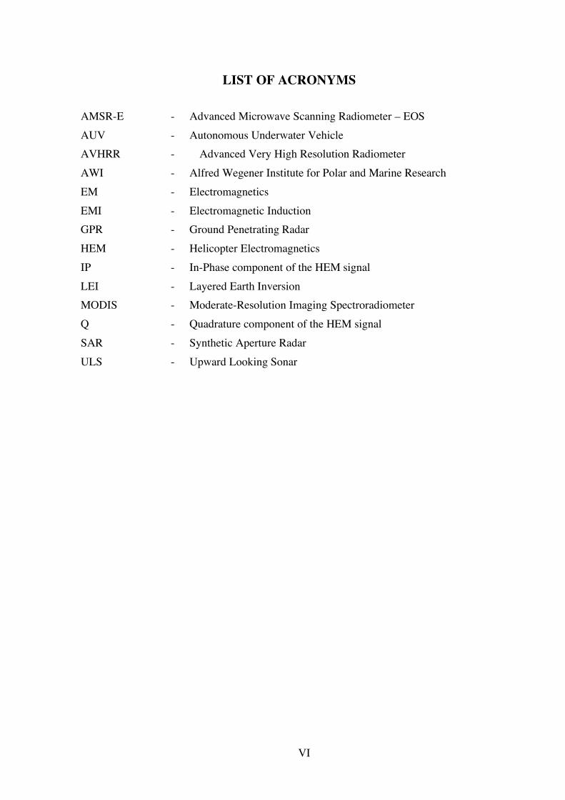
LIST OF ACRONYMS AMSR-E - Advanced Microwave Scanning Radiometer – EOS AUV - Autonomous Underwater Vehicle AVHRR - Advanced Very High Resolution Radiometer AWI - Alfred Wegener Institute for Polar and Marine Research EM - Electromagnetics EMI - Electromagnetic Induction GPR - Ground Penetrating Radar HEM - Helicopter Electromagnetics IP - In-Phase component of the HEM signal LEI - Layered Earth Inversion MODIS - Moderate-Resolution Imaging Spectroradiometer Q - Quadrature component of the HEM signal SAR - Synthetic Aperture Radar ULS - Upward Looking Sonar

1
THESIS

Thesis Andreas Pfaffling
2
HEM sea ice thickness estimation
3
INTRODUCTION
Sea Ice and Climate Change
Frozen sea water “In short words, sea ice is Ocean you can walk on”
Dr. Robert A. Massom, sea ice scientist
When sea water freezes at temperatures normally below –1,86°C sea ice is formed. Passing various age and thickness classes like grease, frazile, pancakes, nilas, first year, and consequently multi year ice the sea ice layer eventually ends up as drifting pack ice, the ice type of importance for the following considerations. Pack ice is a dynamic system floating on the polar oceans influenced by wind and ocean currents. It is composed of level ice floes merged by pressure ridges as well as separated by cracks, leads or several hundred meter wide polynyas. Pressure ridges can exceed 10 m thickness, while level ice hardly grows thicker than 3 meter. Level ice thickness mainly depends on the thermodynamic growing conditions while pressure ridges are linked to short term dynamic events like storms. Then level ice is destroyed and piled up forming delineated tectonic features.
While sea water is generally saline (neglecting low salinities in areas influenced by fresh water intake from rivers) sea salt can not be incorporated into ice crystals. Consequently brine is expelled during ice growth as cold and dense water that sinks to the ocean bottom and is fundamental in driving ocean circulation patterns. Some of the expelled brine is trapped into inclusions in the ice, thus young ice may have a bulk salinity of 2-5 psu (Cox and Weeks, 1974). Bulk salinity refers to the measured salinity of melted ice core samples. During the aging process of sea ice, especially during the melting season, the remaining brine is drained out of the ice through brine channels either by gravity or fresh water flushing from melted snow on the ice surface. Second year or multi-year ice can almost be treated as fresh water ice. Brine inclusions and brine channels have a profound effect on the electromagnetic properties of sea ice (Notz et al., 2005). Detailed investigations on sea ice in general have been documented by Untersteiner (1986) or recently Thomas and Dieckmann (2003).
Sea Ice as a Climate Change indicator “Just as miners once had canaries to warn of rising
concentrations of noxious gases, researchers working on climate change rely on arctic sea ice as an early warning system”
ACIA, 2004
Especially Arctic sea ice is an indicator of climate change (ACIA, 2004) but rather than merely being an indicator, sea ice profoundly influences the global climate due to a number of reasons (e.g. Singarayer et al., 2006):
(1) Sea Ice thickness and concentration governs the flux of heat, moisture and gases between ocean and atmosphere (Singarayer et al., 2006). The more the ice cover shrinks the more open water area is available to release heat from the warm ocean to the atmosphere. Sea ice acts like a lid on the ocean, basically covering the whole polar oceans in winter.
Thesis Andreas Pfaffling
4
(2) Extent and concentration of sea ice determines the albedo (ratio of incoming and reflected solar radiation) in polar regions and cumulatively for the whole globe. Less ice concentration or extent reduces the albedo, which induces further warming of the surface waters and accelerated ice melt - a dangerous positive feedback mechanism. However, it is the top-of-atmosphere albedo that is the most important for warming the planet, and other factors, such as clouds, might confound the simple relationship between ice cover and albedo (Gorodetskaya et al., 2006).
(3) Annual freezing and melting of the seasonal sea ice zone and the consequent release of cold, saline water in winter and fresh water during summer melt is one of the pumps driving the global thermohaline ocean circulation (Saenko et al., 2004).
The role of sea ice in the global climate system is still heavily discussed amongst climate scientists, as the involved interactions are highly complex and difficult to assess. However, observations, models and predictions agree that the Arctic sea ice is shrinking in extend (Cavalieri et al., 2003; Stroeve et al., 2005; Francis et al., 2005) as well as thickness (Rothrock et al., 1999; Vinnikov et al., 1999; Yu et al., 2004, Haas, 2004). Numerical models predict a further decrease of the summer Arctic ice extent due to a longer melt period while it will remain nearly unchanged during winter. For the summer season some models even go as far as predicting an ice free Arctic by 2070 (ACIA, 2004).
Sensors & methods in sea ice research “The church says the earth is flat, but I know that it is
round, for I have seen the shadow on the moon, and I have more faith in a shadow than in the church”
Ferdinand Magellan, explorer
As a matter of fact in today’s high-tech world, the only way to get rock-solid sea ice data is still embarking on a polar research vessel and stepping out on the ice to take samples, perform drillings and carry out observation from the ship. Luckily however, there is a number of geophysical and remote sensing techniques, providing us with more or less accurate estimates of sea ice related quantities. An important descriptor of the ice cover, and its effect on atmosphere-ocean interaction processes and vice versa, is the ice thickness distribution (Thorndike et al., 1975). Accurate information on the ice thickness distribution is essential for quantifying its mass balance and a compendium of methods to determine it are listed in the following. The mentioned examples are a brief list to give the reader a general overview. Especially in the passive and active microwave field further techniques exist than shown here. An excellent review of the state of art in sea ice remote sensing has recently been compiled by Lubin and Massom (2006).
Upward looking sonar Starting as early as 1957, upward looking sonar (ULS) constituted the first regional
sea ice draft information generally gained from tactical Navy submarines (Williams et al., 1975). Those regional, often trans-Polar data sets led to the first hypotheses about thinning sea ice in the Arctic (Rothrock et al., 1999). However Navy missions were sparse in time and location and obviously could not be planned according to scientific needs.
With the use of multi beam sonar (Wadhams, 1978), especially when mounted on autonomous underwater vehicles (AUV), a big step forward in ULS technology was
HEM sea ice thickness estimation
5
achieved (Wadhams et al., 2006). Retrieved sonar swath data, rather than the traditional 1D line, literally gives a new dimension to sea ice draft studies. The shape of the sub-ice surface can be studied in outstanding detail, having a resolution not met with any other method.
Additionally to ULS on moving platforms also ULS moorings have been deployed in areas with continuous sea ice flux like Fram Strait or the Weddell Sea. Investigating the properties of the ice pack drifting over the mooring site can provide volume flux (Drinkwater et al., 2001) or seasonal variability (Worby et al., 2001). Upward looking, bottom mounted ‘acoustic Doppler current profilers’ can also be utilized to retrieve sea ice draft, even though they are usually deployed for oceanographic reasons (Shcherbina et al., 2005).
However, the quantity measured by ULS, whether moving or not, is acoustic travel time which is transferred to sea ice draft. Further presuming a known ice + snow density a sea ice thickness estimate can be derived. Sources of error contain atmospheric pressure changes, sound speed variations, finite signal beamwidth and obviously the assumed ice and snow densities plus snow thickness. An additional problem is the unique definition of the open water reference.
Passive Microwave Radiometers Microwave radiometers are the “classic” sea ice remote sensing tool. First satellites
equipped with microwave radiometers were launched in the late 1970s and since then have been providing a time series of ice extend and concentration on a daily basis (Gloersen et al., 1984). There have been discussions about the ice concentration accuracy in respect to the different processing algorithms revealing significant disagreements of up to 45% in ice concentration (Burns, 1993; Comiso et al., 1997). However, microwave sea ice extent is a reliable data set used for climate studies as well as model validations (Parkinson and Cavalieri, 2002). Microwave radiometer sea ice concentration products have a resolution of 25 km or 12 km depending on the utilized sensor/frequency and algorithm. The most striking advantage of passive microwave measurements is that they penetrate through cloud cover and polar darkness and consequently are able to supply year round data.
Since 2002 with the launch of a modernized sensor, the Advanced Microwave Scanning Radiometer (AMSR-E) onboard NASA’s Aqua satellite (2002-present) and the Japanese satellite ADEOS II (2002-2003), two new products have been added. These are sea ice temperature and snow cover thickness on sea ice (Markus and Cavalieri, 1998; Comiso et al., 2003). Both estimates are still undergoing validation and calibration (Cavalieri and Comiso, 2000, Massom et al., 2006).
Even an attempt to retrieve ice thickness from AMSR-E snow thickness data has recently been presented by Markus (2006) assuming zero freeboard and known snow and ice density. Though various approximations go into this model, regional ice thickness pattern can be described reasonably.
Optical remote sensing Microwave instruments do not directly collect data on albedo or temperature from sea
ice, though this information is important during the spring-summer-autumn seasons to help analyze energy exchange of sea ice. Measurements of sea ice albedo and temperature are possible with spectral optical sensors such as the Advanced Very High Resolution Radiometer (AVHRR, Key and Haefliger, 1992) or Moderate-Resolution
Thesis Andreas Pfaffling
6
Imaging Spectroradiometer (MODIS) instruments. For cloud free scenes the comparably higher resolution of optical remote sensing (25-100 m for MODIS, 1.1-1.5 km for AVHRR, 12.5-50 km for AMSR-E) can be used to determine sea ice extent, temperature, albedo, movement, type, and concentration (Riggs et al., 1999). Further sea ice surface temperature can relate to sea ice thickness for thin ice since the thicker the ice, the colder the surface (Yu and Rothrock, 1996).
Synthetic Aperture Radar In contrast to most of the other discussed methods, Synthetic Aperture Radar (SAR)
deals with the radar backscatter from the ice surface which is mainly determined by the surface roughness (amongst other parameters like the electromagnetic properties of the ice). Consequently SAR is mainly used for ice classifications, e.g. first year / multi year ice discrimination (Kwok et al., 1992; Fetterer et al., 1994; Breivik et al., 2001; Kwok, 2004). However, SAR data is available in very high resolution down to 25 meter, making it a perfect tool for high resolution spatial investigation (pressure ridges, leads, etc.) or for navigational purposes. SAR data may be used in combination with AVHRR data for higher resolution and accuracy of optical products as described earlier.(Hauser et al., 2001).
Basing on initial investigations by Kwok et al. (1995) latest research indicates a possibility to retrieve thin ice thickness (< 50 cm) from radar backscatter co-polarization ratio acquired with a helicopter borne multi-frequency, multi-polarization scatterometer (Kern et al., 2006). Results seem promising and further developments are ongoing. Though no satellite data of this kind is available yet, several missions are planned to launch in 2006/07 which may provide data to test the thin sea ice algorithm.
Radar & laser altimeters Nowadays altimeters are the only space borne sensors, attempting to measure sea ice
thickness from space for all ice types. However, comparable to the challenges for ULS where draft needs to be transferred to thickness, altimeters can only retrieve freeboard measurements which lead to ice thickness. On of the challenges of altimeter freeboard estimation is the accurate knowledge of the sea level reference. Furthermore the poorly known snow thickness can introduce significant bias to the retrieved sea ice thickness (ESA, 2001). Further complication arises due to the very small freeboard values (~ a tenth of the thickness) demanding high accuracies. Despite all these challenges, first cryosphere - dedicated altimeter space missions (ICESat, CryoSat) as well as altimeters on existing satellites like ENVISAT and ERS lead to first reasonable results (Kwok et al., 2006). ICESat launched by NASA in 2003 relies on a laser altimeter and consequently retrieves the snow surface freeboard, also called surface elevation (Kwok et al., 2004). In contrast the European approach counts on radar altimeters such as on ENVISAT or ERS as well as ESA’s Cryosphere dedicated mission CryoSat to be (re)-launched in 2009 (Drinkwater et al., 2004). Due to the penetration of the radar pulse, the radar – determined freeboard describes the true ice freeboard, in contrast to the laser determined surface elevation. First investigations of space-borne altimeter sea ice thickness data focus on interannual variability derived from past ERS data (Laxon et al., 2003), sea ice model optimizations (Miller et al., 2006) as well as ice volume flux studies (Kwok et al., 2005; Spreen et al., 2006).
HEM sea ice thickness estimation
7
Geophysical solutions The well established geophysical method of electromagnetic (EM) induction (Ward et
al., 1988) is the only method capable of directly measuring sea ice (plus snow) thickness on regional scales. The technique is described in detail in the following sections, thus some examples of additional geophysical methods are briefly lined up here.
Resistivity sounding has been used for in situ studies of sea ice properties (Thyssen et al., 1974) and lately emphasising on conductivity anisotropy and its role for Helicopter EM sea ice thickness profiling (paper IV). In contrast to the one-dimensional character of resistivity sounding, recently resistivity tomography has been performed across pressure ridges in the Arctic and Baltic Seas to illuminate the internal structure of keel ridges (Flinspach, 2005).
Ground penetrating radar (GPR) has been used for snow and/or ice thickness profiling with varying prosperity both from the ground (Kovacs, 1978; Otto, 2004) and helicopter borne (Lalumiere, 1998). Brine inclusions in sea ice can cause high attenuation and scattering for the high frequency radar signals. Consequently cold multi year sea ice possesses the highest likelihood for successful GPR profiles. However, the mentioned limitations are valid for commercially available impulse radars with limited bandwidth. Recent developments lead to broadband radars dedicated for snow and sea ice thickness retrieval, which might overcome the problems met with traditional GPR (Jezek et al., 1998, Gogineni et al., 2003). Nevertheless also nowadays GPR systems perform well for snow thickness mapping.
The need for a direct sea ice thickness measure “It is difficult to say what is impossible, for the dream of yesterday is the hope of today and the reality of tomorrow”
Robert H. Goddard, rocket scientist
Resuming the characteristics of all oceanographic and remote sensing methods mentioned so far, underlines that none of them is able to directly measure sea ice thickness. Recordings such as sea ice draft, sea ice- or snow- freeboard, thin sea ice surface temperature or radar backscatter are transferred to sea ice thickness estimates with the help of assumptions and approximations. Though those thickness estimates can provide large scale information, they depend on ground truth data to tune and validate the used algorithms. Further the next challenge is how to relate a hand full of drillings to the size of satellite pixels or how to deal with the variability of thickness or ice concentration within one pixel. To tackle this problem, geophysical methods such as EM profiling can provide an excellent mid scale calibration / validation data set for sea ice thickness (Prinsenberg et al., 1996; Peterson et al., 1999; Kern et al., 2006; Pfaffling et al., 2006).
Introducing EM for sea ice thickness profiling Initial work using a surface-based EM induction system goes back to the 1970s
(Sinha, 1976) and this work showed the effectiveness of this approach in principle. Additional work led to a system based on the Geonics EM-31 ground conductivity meter (McNeil, 1980; Kovacs and Morey, 1991), since then being used on an operational basis on the ice surface as well as suspended from ship cranes (Prinsenberg et al., 1996; Peterson et al., 1999; Haas et al., 1997; Haas, 1998). Due to its semi-regional applicability, ground based EM has been used to study changes in the regional
Thesis Andreas Pfaffling
8
sea ice thickness distribution as reported by Haas (2004). However, using EM instruments on the ice or from ships introduces a certain bias to the determined ice thickness distribution. Man-hauled instruments will stay clear of any thin ice areas and definitely open water, while ship borne devices will hardly sense really thick ice, as ice breaker officers tend to navigate in leads or rather thinner ice areas. Consequently the EM thickness distribution either lacks thin or thick ice. However, both scenarios can be overcome once the system is used from an airborne platform.
Airborne EM spreads out Regional mapping of the sea ice thickness distribution using helicopter
electromagnetics (HEM) began in the late eighties in north America with traditional exploration systems (Kovacs et al., 1987) leading to sea ice dedicated devices (Kovacs and Holladay 1990; Kovacs et al., 1995). Technology was further developed in Canada (Holladay et al., 1990; Peterson et al., 1999; Prinsenberg et al., 2002) prior to research in Europe since the early 1990’s. The first European airborne EM sea ice field program was conducted in the Baltic sea using the Geological Survey of Finland’s fixed wing EM system (Multala et al., 1996). The latest European development was initiated in 2000 by the Alfred Wegener Institute for Polar and Marine Research (AWI). The AWI HEM system is a small scale, purpose built, adaptable, fully digital instrument which has been used on an operational basis during ship and land based expeditions in the Arctic, Antarctic and Baltic seas (Pfaffling et al., 2004; Haas et al., 2006; paper II).
Principle of HEM sea ice thickness retrieval Frequency domain, dual loop electromagnetic induction (EMI) is a geophysical
technique, developed to find conductive targets for mineral exploration (Frischknecht et al., 1988). Small, single frequency instruments such as the EM-31 were designed for anomaly hunting rather than vertical conductivity sounding. In contrast, modern exploration HEM instruments with up to six frequencies (Fugro’s RESOLVE system, Smith et al., 2003) deliver detailed conductivity-depth-images via geophysical inversion (Paterson and Redford, 1986; Sengpiel and Siemon, 1998). Although single-frequency EM rules out frequency sounding, measured EM field can be related to ice thickness given the simple model dimensionality. In a nutshell, EMI provides a measure on the conductivity and distance of any conductor within range of the emitted EM-field. This “conductor ranging” capability makes EM capable for sea ice thickness retrieval.
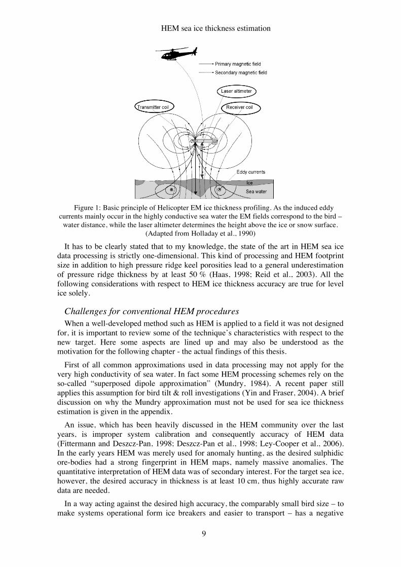
Being saline, sea water is a good conductor (2.5 - 3 S/m) and therefore provides a strong HEM response. In contrast, sea ice has a low conductivity around 0.01 S/m, thus the measured EM response depends mainly on the height of the system above the seawater. It is consequently possible to directly explore ice thickness with an airborne EM instrument. The basic principle of HEM sea ice thickness profiling is to estimate the distance to the ice / water interface from the EM data, while a laser altimeter in the towed instrument (bird) determines the system height above the ice or snow surface (figure 1). The difference of these two distances consequently corresponds to the ice (or ice + snow) thickness. Whenever sea ice thickness is mentioned in an EM context, it actually refers to the total thickness meaning ice thickness plus snow thickness. A detailed description of the AWI HEM system and ice thickness retrieval is given by Haas et al. (2006) and paper II.
HEM sea ice thickness estimation
9
Figure 1: Basic principle of Helicopter EM ice thickness profiling. As the induced eddy
currents mainly occur in the highly conductive sea water the EM fields correspond to the bird – water distance, while the laser altimeter determines the height above the ice or snow surface.
(Adapted from Holladay et al., 1990)
It has to be clearly stated that to my knowledge, the state of the art in HEM sea ice data processing is strictly one-dimensional. This kind of processing and HEM footprint size in addition to high pressure ridge keel porosities lead to a general underestimation of pressure ridge thickness by at least 50 % (Haas, 1998; Reid et al., 2003). All the following considerations with respect to HEM ice thickness accuracy are true for level ice solely.
Challenges for conventional HEM procedures When a well-developed method such as HEM is applied to a field it was not designed
for, it is important to review some of the technique’s characteristics with respect to the new target. Here some aspects are lined up and may also be understood as the motivation for the following chapter - the actual findings of this thesis.
First of all common approximations used in data processing may not apply for the very high conductivity of sea water. In fact some HEM processing schemes rely on the so-called “superposed dipole approximation” (Mundry, 1984). A recent paper still applies this assumption for bird tilt & roll investigations (Yin and Fraser, 2004). A brief discussion on why the Mundry approximation must not be used for sea ice thickness estimation is given in the appendix.
An issue, which has been heavily discussed in the HEM community over the last years, is improper system calibration and consequently accuracy of HEM data (Fittermann and Deszcz-Pan, 1998; Deszcz-Pan et al., 1998; Ley-Cooper et al., 2006). In the early years HEM was merely used for anomaly hunting, as the desired sulphidic ore-bodies had a strong fingerprint in HEM maps, namely massive anomalies. The quantitative interpretation of HEM data was of secondary interest. For the target sea ice, however, the desired accuracy in thickness is at least 10 cm, thus highly accurate raw data are needed.
In a way acting against the desired high accuracy, the comparably small bird size – to make systems operational form ice breakers and easier to transport – has a negative
Thesis Andreas Pfaffling
10
effect on sensitivity and thus signal to noise ratio and consequently on the accuracy. This “Bermuda triangle” of desired accuracy – instrument noise – system sensitivity needs detailed investigation to give reasonable accuracy information for the delivered ice thickness data, both in respect to calibration as well as the small bird size.
Geophysical inversion is a complex topic. It has become an industry standard to feed HEM datasets through layered earth inversion and compile resistivity maps and cross-sections (Sengpiel and Siemon, 1998, Constable et al., 1987, Huang and Fraser, 1991). This method, however, relies on multi-frequency datasets and can not be transferred to two-frequency sea ice systems in a straight forward way. At Bedford Institute of Oceanography specifically tuned, on board – real time inversion appears to be used for their sea ice HEM system. (not published, stated in internal reports at their website www.mar.dfo-mpo.gc.ca/science/ocean/seaice/intro_e.html). Yet this scheme can not be applied for the AWI device without prior analytic assessment due to the different system properties. It is a fundamental question how the rather exotic suite of frequencies (3.6 kHz and 112 kHz) and even more contrasting conductivities (sea ice 50 mS/m and sea water 2-4 S/m) effect layered earth inversion, which normally deals with a quite uniform set of frequencies and a smooth conductivity model.
Today’s common inversion codes perform so called stitched one-dimensional (1D) inversions. This means that for any data point a 1D inversion is computed and then the results are stitched to a continuous profile. Auken and Christiansen (2004) introduced a 1.5-D inversion where the single 1D inversions are spatially constrained, which almost leads to a 2D inversion quality. Full-scale 3D inversion codes are about to enter the market (Raiche, 2001; Sasaki, 2001; Zhang, 2003). Liu and Becker (1990) have discussed the possibilities for 2D HEM sea ice thickness processing with interpretation charts and elaborate 2D inversion (Liu et al., 1991) with promising results. Yet improvements where minor compared to the extensive computing needed, making 2D processing not operational at the time this thesis is written. However, as generally 1D processing is used for the sea ice case, it is substantial to find out about the precise footprint size of the induction system, to get an estimate on the spatial size of sea ice features, resolvable by 1D processes HEM data.
Last but not least it is of profound importance to know the conductivity characteristics of sea ice as detailed as possible. Most of the sea ice conductivity estimates used, are based on the salinity of melted core samples. Bearing in mind the destruction of the complex inner structure of brine cells in sea ice, melting cores can only be a first estimate.
HEM sea ice thickness estimation
11
ADAPTING HELICOPTER ELECTROMAGNETICS FOR SEA ICE
This chapter briefly reviews the key findings of the papers in this thesis. For further descriptions and discussions please refer to attached papers, which are quoted by their Roman numerals.
Precision / accuracy preamble Sometimes there is confusion and disbelieve about the proper usage of the terms
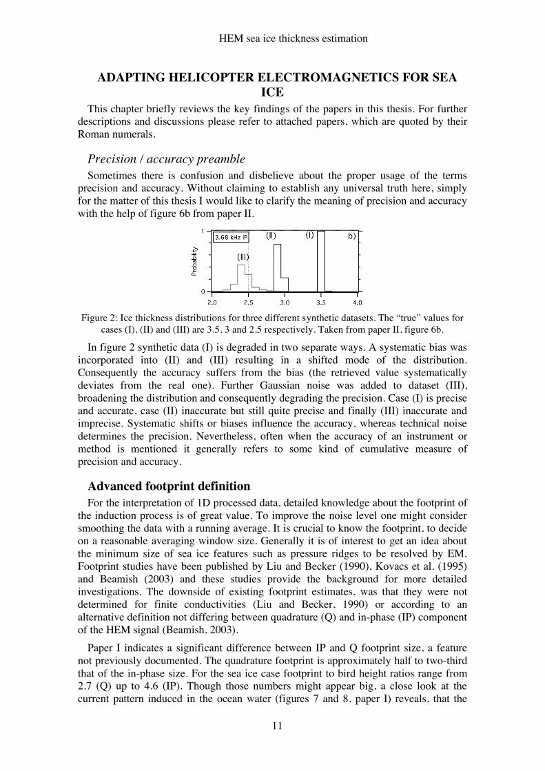
precision and accuracy. Without claiming to establish any universal truth here, simply for the matter of this thesis I would like to clarify the meaning of precision and accuracy with the help of figure 6b from paper II.
Figure 2: Ice thickness distributions for three different synthetic datasets. The “true” values for
cases (I), (II) and (III) are 3.5, 3 and 2.5 respectively. Taken from paper II, figure 6b.
In figure 2 synthetic data (I) is degraded in two separate ways. A systematic bias was incorporated into (II) and (III) resulting in a shifted mode of the distribution. Consequently the accuracy suffers from the bias (the retrieved value systematically deviates from the real one). Further Gaussian noise was added to dataset (III), broadening the distribution and consequently degrading the precision. Case (I) is precise and accurate, case (II) inaccurate but still quite precise and finally (III) inaccurate and imprecise. Systematic shifts or biases influence the accuracy, whereas technical noise determines the precision. Nevertheless, often when the accuracy of an instrument or method is mentioned it generally refers to some kind of cumulative measure of precision and accuracy.
Advanced footprint definition For the interpretation of 1D processed data, detailed knowledge about the footprint of
the induction process is of great value. To improve the noise level one might consider smoothing the data with a running average. It is crucial to know the footprint, to decide on a reasonable averaging window size. Generally it is of interest to get an idea about the minimum size of sea ice features such as pressure ridges to be resolved by EM. Footprint studies have been published by Liu and Becker (1990), Kovacs et al. (1995) and Beamish (2003) and these studies provide the background for more detailed investigations. The downside of existing footprint estimates, was that they were not determined for finite conductivities (Liu and Becker, 1990) or according to an alternative definition not differing between quadrature (Q) and in-phase (IP) component of the HEM signal (Beamish, 2003).
Paper I indicates a significant difference between IP and Q footprint size, a feature not previously documented. The quadrature footprint is approximately half to two-third that of the in-phase size. For the sea ice case footprint to bird height ratios range from 2.7 (Q) up to 4.6 (IP). Though those numbers might appear big, a close look at the current pattern induced in the ocean water (figures 7 and 8, paper I) reveals, that the
Thesis Andreas Pfaffling
12
majority of eddy currents actually is induced in a doughnut shaped area about half the size of the footprint estimates. Equipped with the mathematical definition of the “shape” of the footprint (figure 12a, paper I), field data could be fed through a running weighted average according to the footprint shape. Comparing such averages with field data, was not completely convincing though general features agreed. Most likely 3D under-sampling of the available drilling data was the cause. However, the predicted smaller footprint for the quadrature is also found in the field data. To study resolvable pressure ridge dimensions, 3D models were run with respect to footprint size. Results imply that ridges have to be separated at least one footprint to be distinguished as single features. Or to saddle the horse from the back – the footprint size is the minimum lateral extend of a feature, so that the retrieved EM thickness would be correct. As most pressure ridges are smaller than the footprint size, their maximum thickness is underestimated and the lateral thickness profile smeared out.
System calibration & precision High quality calibration and low noise level belong to the most crucial variables to
assure useful data (Deszcz-Pan et al., 1998; Ley-Cooper et al., 2006). The industry standard for HEM calibration until very recently was ground based calibration on resistive geology with handheld calibration coils and phasing bars (Fitterman, 1998). Lately onboard calibration units, running calibration sequences at high altitude, were a big step forward to better calibration quality (Hodges, 2001; Haas et al., 2002). System noise is mainly caused by electronic parts and mechanical vibrations. It should be mentioned that a significant advantage of having an own system is the actual access to the raw noise levels. In contrast, contractors usually filter and smooth data before delivery and supply their corporate noise estimates.
Calibration The frequently met open water areas when operating in Polar seas provide us with the
unique opportunity to perform calibration checks on almost every flight. EM data acquired over open water is assessed with synthetic model curves and if required, calibration gain and phase values can be adjusted. In the case of the uniquely simple “geology” of the sea ice case, post-flight calibration can even go one step further: Emphasizing on amplitude and phase of the measured electromagnetic field rather than quadrature and in-phase, it becomes evident that EM-amplitude depends on system height and EM-phase on ground conductivity (Sinha, 1973). The influence of the thin sea ice layer on the cumulative apparent conductivity of the half-space is small. Thus modelled HEM response for open water compared to sea ice covered water hardly differs in EM-phase. This means that even at operational altitude over the target, phase calibration can be corrected with model curves if in doubt (figure 6, paper III). This is a very handy feature, as especially system phase tends to drift much more than system gain.
Precision is noise divided by sensitivity Noise is a technical term, usually expressed in ppm (the unit of the measured EM
field). Contrarily precision is desired in cm ice thickness. The variable connecting these values is the system’s sensitivity [ppm/m]. It basically expresses for how many ppm the simulated measurement would change if for example the ice would be 5 cm thicker (sensitivity with respect to ice thickness). Sensitivity can be defined with respect to any factor influencing the simulated measurement (bird height, water conductivity, ice
HEM sea ice thickness estimation
13
conductivity, frequency, transmitter – receiver spacing, …). However, here I emphasis on ice thickness sensitivity. Given the noise as a technical parameter, the sensitivity is the key value to understand what the effect on the actually measured ice thickness is. Paper II includes a very detailed discussion on system sensitivity for a variety of frequencies, transmitter-receiver spacings (= coil spacing), sea water conductivities and bird altitudes. An interesting detail is that the in-phase and quadrature components show different sensitivity patterns in the frequency vs. coil spacing domain. While the IP sensitivity continuously rises with frequency as well as coil spacing, there is an optimum frequency for the Q sensitivity while it also rises with coil spacing. A trade off has to be found in instrument design. Comparing traditional exploration birds with sea ice dedicated systems reveals that a sea ice bird has to fly at 15 m height to gain the same sensitivity as an exploration bird at 30 m. Generally conditions for small birds are tough: For a noise level of 5 ppm and a desired sea ice thickness precision of 10 cm the system must be flown at less than 16 m height. Luckily there are few high obstacle scattered on sea ice, making it possible to fly so low.
Sea ice conductivity, target or bias? Knowledge about the inner conductivity structure of sea ice is important for several
reasons. Sea ice is not a homogeneous layer with a representative conductivity. Level ice has a typical conductivity profile with higher conductivities on the top and bottom and lower values in-between (Thomas and Dieckmann, 2003). The conductivity of sea ice arises from the enclosed brine pockets and channels and consequently follows their geometry (Timco, 1979). Furthermore, when considering pressure ridges the role of porosity is profound as ridges are merely a pile of ice blocks with extended water volumes in-between. This is one of the reasons why the maximum pressure ridge thickness can not be measured by EM induction.
Sea ice is anisotropic In situ measurements of sea ice conductivity with the help of resistivity sounding
reveals the strong vertical / horizontal anisotropy of level sea ice (paper IV). The dominantly vertically orientated brine channels are the cause for the observed anisotropy. As sea ice conductivity is ruled by brine, vertical conductivity is 9 to 12 times higher than the horizontal component. Ice conductivity from melted cores (bulk conductivity) lays in-between those extremes. This is a significant finding for EM modelling, as inductively coupled eddy currents are strictly horizontal due to the infinite conductivity contrast between air and conductor (ice or water). Consequently the bulk conductivity must be considered as an over-estimate for EM sea ice sensitivity studies.
The accuracy of an approximation Due to the large conductivity contrast between sea ice and sea water and the relatively
thin sea ice layer the induced EM fields are mainly governed by the sea water conductivity. For this reason the sea ice conductivity is neglected in the HEM sea ice thickness processing algorithm as discussed in paper II. This approximations simplify the complex geophysical inversion procedure to a simple direct inversion approach (look-up table). The algorithm is fast, stable and unambiguous, yet slightly degrades the accuracy due to the approximations involved. Numerical studies to quantify this effect show that a desired accuracy of 10 cm is achieved for level ice thinner than 3 m for standard ocean water (Arctic, Antarctic) and conductive ice (50 mS/m). However, ice of 3 m or more would mostly be multi-year ice, which has lost most of its brine and thus a
Thesis Andreas Pfaffling
14
much smaller conductivity than the used 50 mS/m. Consequently it can be stated that direct inversion remains within the desired accuracy for conductive ice up to 3 m. Further there is no accuracy problem with thicker ice due to its smaller conductivity. For brackish water sea ice as met in the Baltic sea the effect is neglectable.
Data quality versus inversion Though the simplified direct inversion algorithm appears to work well (paper II),
formal geophysical inversion would have the potential to provide more information (paper III). Besides the fact, that the zero sea ice conductivity assumption would become redundant, sea ice conductivity might actually be retrieved from the EM dataset. Incorporating sea ice conductivity in the inversion process would avoid possible biased thickness results when extreme sea ice conductivities are met. Mostly Antarctic phenomenons such as surface flooding, or porous gap layers result in an abnormal sea ice conductivity, which would bias the look-up-table results. For potential adoption of existing inversion codes for sea ice thickness determination, the general performance of inversion codes has to be assessed, given the unique set of frequencies and model parameters.
Inversion studies on synthetic data reveal the capability of layered – earth – inversion (LEI) to retrieve ice thickness in comparable quality as with the direct approach (paper III). However, it is evident that inverted sea ice conductivity results are unstable for thickness less than 2 m. An unfortunate result, as inverted conductivity could distinguish between first year and multi year ice, which is mostly redundant for ice at thickness of 3 m and more. Nevertheless LEI successfully accounts for high sea ice conductivities, where the direct algorithm would be biased towards smaller thickness. Taking LEI one step further and also inverting for water depth (three layer model) successfully retrieves water depths up to 25 m. The synthetic data for this bathymetry example is computed for brackish water, as shallow water is frequently in this environment. Finally a 3D synthetic data set undergoes 1D inversion to investigate the capability to retrieve keel conductivity. LEI keel conductivity results are elevated with respect to the surrounding level ice regardless if the original 3D model involved high conductivities or not. The 3D artefacts in the LEI results mask effects from changes in the model keel conductivity.
Inversion of a field data set confirms the findings from analyzed synthetic data. For a small ice thickness of half a meter the inverted ice conductivity is arbitrary. System noise exceeds the very small sensitivity with respect to sea ice conductivity. Thickness results are reasonable but worse than direct inversion results. A misfortunate combination of noise levels and diverging sensitivity is suspected to be the cause.
Outlook The findings presented so far are mainly discussions of certain factors influencing the
accuracy and precision of HEM sea ice thickness estimates. It remains to soothsay what could be done to improve the state of the art in HEM sea ice exploration. In the following I will give some recommendations for possible improvements.
The most powerful remaining factor degrading HEM sea ice thickness, is the bird’s attitude, which is not measured by the AWI system and not included into data processing in general. Bird pitch and roll biases the retrieved ice thickness in two ways. The altitude measured by the laser is biased as the laser looks at an angle rather than at nadir. Furthermore the EM induction process is distorted as the receiver and transmitter
HEM sea ice thickness estimation
15
coils change in orientation and position. Recently Fitterman and Yin (2004) as well as Yin and Fraser (2004) showed the profound influence of bird attitude on inversion results for terrain conductivities common in exploration and geological mapping. Over the last years it became a common agreement in the airborne EM community that results can only be accurate, when the exact bird position and attitude is known. With respect to sea ice HEM Holladay and Prinsenberg (1997) presented biased retrieved ice thickness due to bird swing, but could not explain the effect with synthetic examples. However, synthetic data used by Holladay and Prinsenberg had been modelled for an exploration bird at 30 m over a 0.01 S/m half-space, while the field data arose from a small sea ice bird over conductive sea water. Proper analytical modelling of attitude effects will show its importance for sea ice and consequently the need to measure pitch and roll and feed them into the processing algorithm.
The pitfalls of 1D processing and inversion have been addressed several times in this thesis. Usually most 1D inversion papers would conclude with an outlook towards 2D or 3D inversion. For the specific problem of sea ice pressure ridges, I doubt that 2D inversion will ever become operational. It is questionable, if the incomparably higher processing effort would yield sufficiently more or better information. The problem of HEM pressure ridge keel underestimation is twofold. One part is the 1D processing and the consequent smearing-out of 3D features. However, the high porosity of ridge keels, the existence of a consolidated layer followed by a diffuse, piled up mixture of ice blocks and sea water is the much more significant difficulty. 2D inversion would not be able to account for that, unless the number of frequencies used in sea ice HEM systems would be increased. Consequently it’s not enough to just change the processing scheme to resolve pressure ridge keels. A EM system with advanced features would have to be designed for that purpose. However, comparisons of drilled consolidated layer thickness and 1D processed EM ice thickness agree well (unpublished field results, IRIS 2005 campaign).
Finally a suggestion for future HEM sea ice data handling arises from figure 9, paper II in contrast to figure 7, paper III. The same dataset, once presented as total thickness and once as freeboard and draft. As discussed in the papers, the small ridge is not sensed by the EM but rather picked up by the laser altimeter. Consequently the commonly compiled total HEM ice thickness estimates, represent a blending of EM-draft and laser-freeboard. Thus a lot of features in the thickness plot may actually only arise from topography, picked up by the laser. Note that not every sail necessarily has a keel and vice versa. With the recent introduction of a DGPS on board the AWI bird an alternative HEM ice thickness product is conceivable. Basing on an absolute height above sea level (by the DGPS), the laser altitude would supply a high resolution freeboard profile, while the HEM interpretation would yield the draft profile, preferably smoothed using a footprint-weighted running average prior processing.
Thesis Andreas Pfaffling
16
ACKNOWLEDGMENTS Neither last nor least I need to thank my personal sunshine for supporting me in all
those countless ways. Life has been everything but a straight line over the last months and completing this thesis (and who knows what else) would have been seriously in jeopardy without someone to stand by me, motivate me and simply be there for me. Thank you so much!
I am ultimately grateful to James Reidα for being a mentor, colleague and mate at the same time. The geophysical aspects of this work have been stimulated an inspired by his broad knowledge and experience in Airborne EM. It was a pleasure working with him on a short visiting stay in Hobart.
Further acknowledgments go to Christian Haasβ and Prof. Millerγ, who pulled me into sea ice research and enabled me to work on the exciting topic of helicopter borne EM. I’m however still in doubt about what Christian told me in April 2003: “This is a small step for you but a big step for sea ice research”.
Back in the days I stumbled across extremely interesting lectures on the basics of geophysics held by Prof. Burkhardtδ and Prof. Yaramanciδ. I owe the initial spark of interest in geophysics to them. Further the warm and familiar atmosphere at their institute during my time as a master student consolidated my enthusiasm for becoming a geophysicist. Thanks again for a great start.
Further I am grateful for the comforting work atmosphere amongst the sea ice group at AWI, the scientific discussions and all the fun along the way and during the numerous field trips. Special thanks to Marcel and Jan, frequently acting as lightning rods, when anger about administration, funding policy, lack of common sense, etc. set me on fire.
During my time at AWI I participated in expeditions to the Arctic, Antarctic and Baltic in cooperation with project partners from the UK, Australia, Denmark, Finland, and more. All you folks I spent time with on ships and on the ice, it was a pleasure working with you!
The quality of this thesis has been improved by comments from Marian Hertrich, Jan Lieser, Katrine Aspmo and Stefan Kern.
None of this work could have been achieved without the support of ship crews and helicopter teams. Thanks for handling, flying (and fixing) the bird.
Finally last but still not least I’m grateful for my parents support over the hard years and all the private and professional ups and downs.
α Dr. James Reid is lecturer at the School of Earth Science at University of Tasmania. β Dr. Christian Haas is head of the Sea Ice Physics section at AWI. γ Prof. Dr. Heinz Miller is head of the Glaciology section and Deputy Director at AWI δ Prof. Dr. Hand Burkhardt and Prof. Dr. Ugur Yaramanci head the School of Applied Geophysics at the Institute of Applied Geosciences at Technical University Berlin.
HEM sea ice thickness estimation
17
REFERENCES ACIA, 2004, Impacts of a Warming Arctic: Arctic Climate Impact Assessment,
Cambridge University Press, ISBN 0521617782. Auken, E., and A. V. Christiansen, 2004, Layered and laterally constrained 2D
inversion of resistivity data: Geophysics, 69, 752–761. Beamish, D., 2003, Airborne EM footprints: Geophysical Prospecting, 51, 49–60. Breivik, L.-A., S. Eastwood, Ø. Godøy, H. Schyberg, S. Andersen, and R. Tonboe,
2001, Sea Ice Products for EUMETSAT Satellite Application Facility: Canadian Journal of Remote Sensing, 27 (5), 403-410.
Burns, B. A., 1993, Comparison of SSM/I ice-concentration algorithms for the Weddell Sea: Annals of Glaciology, 17, 344-350.
Cavalieri, D., and J. Comiso. 2000. Algorithm Theoretical Basis Document for the AMSR-E Sea Ice Algorithm, Revised December 1, 2000. NASA Goddard Space Flight Center, Greenbelt, MD, USA, 79 pp. (<http://eospso.gsfc.nasa.gov/ftp_ATBD/REVIEW/AMSR/atbd-amsr-seaice.pdf>)
Cavalieri, D. J., C. L. Parkinson, and K. Y. Vinnikov, 2003, 30-Year satellite record reveals contrasting Arctic and Antarctic decadal sea ice variability, Geophysical Research Letters 30(18), 1970, doi:10.1029/2003GL018031.
Comiso, J. C., D. J. Cavalieri, C. L. Parkinson, and P. Gloersen, 1997, Passive Microwave Algorithms for Sea Ice Concentration: A Comparison of Two Techniques: Remote Sensing of the Environment, 60, 357-384.
Comiso, J., D. Cavalieri, and T. Markus, 2003, Sea ice concentration, ice temperature, and snow depth using AMSR-E data: IEEE Transactions on Geoscience and Remote Sensing, 41 (2), 243-252.
Cox, G. F. N., and W. F. Weeks, 1974, Salinity variations in sea ice: Journal of Glaciology, 13, 109-120.
Constable, S. C., R. L. Parker, and C. G. Constable, 1987, Occam’s inversion: a practical algorithm for generating smooth models from electromagnetic sounding data: Geophysics, 52, 289-300.
Deszcz-Pan, M., D. V. Fitterman, and V. F. Labson, 1998, Reduction of inversion errors in helicopter EM data using auxiliary information, Exploration Geophysics, 29, 142-146.
Drinkwater, M. R., X. Liu, S. Harms, 2001, Combined satellite- and ULS-derived sea-ice flux in the Weddell Sea, Antarctica: Annals of glaciology, 33, 125-132.
Drinkwater, M. R., R. Francis, G. Ratier, D. J. Wingham, 2004, The European Space Agency’s Earth Explorer Mission CryoSat: measuring variability in the cryosphere: Annals of Glaciology, 39, 313-320.
European Space Agency (ESA), 2001, CryoSat calibration and validation concept: Noordwijk, European Space Agency, (CS-PLUCL-SY-0004.) (<http://esamultimedia.esa.int/docs/Cryosat/CVC_14Nov01.pdf >)
Fetterer, F., D. Gineris, and R. Kwok, 1994, Sea ice type maps from Alaska synthetic aperture radar facility imagery: An asessment: Journal of Geophysical Research, 99 (C11), 22,443-22,458.
Thesis Andreas Pfaffling
18
Fitterman, D. V., 1998, Sources of calibration errors in helicopter EM data: Exploration Geophysics, 29, 65-70.
Fitterman, D. V., and M. Deszcz-Pan, 1998, Helicopter EM mapping of saltwater intrusion in Everglades National Park, Exploration Geophysics, 29, 240 – 243.
Fitterman, D. V., and C. Yin, 2004, Effect of bird maneuver on frequency-domain helicopter EM response: Geophysics, 69, 1203-1215.
Flinspach, D., 2005, Gleichstromgeoelektrik zur Erkundung der inneren Struktur und der Dicke von Meereis. Masters Thesis (in German), Ludwig-Maximilians-Universität München, Germany.
Francis, J. A., E. Hunter, J. R. Key, and X. Wang, 2005, Clues to variability in Arctic minimum sea ice extent: Geophysical Reseatch Letters, 32, L21501, doi:10.1029/2005GL024376.
Frischknecht, F. C., V. F. Labson, B. R. Spies, and W. L. Anderson, 1988, Profiling methods using small sources, in M. N. Nabighian, ed., Electromagnetic methods in applied geophysics, Vol. 1, Theory, 131-311: Society of Exploration Geophysicists, ISBN 1-56080-069-0.
McNeil, J. D., 1980, Electromagnetic terrain conductivity measurement at low induction numbers, technical note tn-6, Geonics, Ltd., Mississauga, Ontario, Canada.
Gloersen, P., D. J. Cavalieri, A. T. C. Chang, T. T. Wilheit, W. J. Campbell, O. M. Johannessen, K. B. Katsaros, K. F. Kunzi, D. B. Ross, D. Staelin, E. P. L. Windsor, F. T. Barath, P. Gudmansen, E. Langham, and R. Ramseier, 1984, A summary of results from the first Nimbus-G SMMR observations, Journal of Geophysical Research 89:5335-44.
Gogineni, S, K. Wong, S. Krishnan, P. Kanagaratnam, T. Markus, and V. Lytle. 2003. An ultra-wideband radar for measurements of snow thickness over sea ice. Proc. Int. Geosc. Rem. Sens. Symp., IGARSS ’03, 4, 2802-2804.
Gorodetskaya, I. V., M. A. Cane, L.-B. Tremblay, and A. Kaplan, 2006, The Effects of Sea-Ice and Land-Snow Concentrations on Planetary Albedo from the Earth Radiation Budget Experiment: Atmosphere-Ocean, 44 (2), 195-205.
Haas, C., S. Gerland, H. Eicken, and H. Miller, 1997, Comparison of sea- ice thickness measurements under summer and winter conditions in the Arctic using a small electromagnetic induction device: Geophysics, 62, 749–757.
Haas, C., 1998, Evaluation of ship-based electromagnetic-inductive thickness measurements of summer sea ice in the Bellingshausen and Amundsen seas, Antarctica: Cold Regions Science and Technology, 27, 1–16.
Haas, C. 2004, Late-Summer Sea Ice Thickness Variability in the Arctic Transpolar Drift 1991-2001 derived from ground-based Electromagnetic Sounding: Geophysical Research Letters, 31, L09402, doi:10.1029/2003GL019394.
Haas, C., H. Edeler, M. Schürmann, J. Lobach, and K.-P. Sengpiel, 2002, First operation of AWI HEM-bird for sea-ice thickness sounding: Proceedings, 62. Jahrestagung der Deutschen Geophysikalischen Gesellschaft DGG, 36-38.
Haas, C., Goebell, S., Hendricks, S., Martin, T., Pfaffling, A., and von Saldern, C., 2006. Airborne electromagnetic measurements of sea ice thickness: methods and applications, in European Commission, Arctic Sea Ice Thickness: Past, Present &
HEM sea ice thickness estimation
19
Future, edited by Peter Wadhams and Georgios Amanatidis, Climate Change and Natural Hazards Series, Brussels, 2006.
Hauser, A., L. Mathew, and G. Wendler, 2002, Sea-Ice Conditions in the Ross Sea during Spring 1996 as observed on SAR and AVHRR Imagery, Atmosphere-Ocean, 40 (3), 281–292.
Hodges, G., 2001, Calibration of the DIGHEM Digital (DSP) System: technical note, Fugro Airborne Surveys, available online (<http://www.fugroairborne.com.au /resources/technical_notes/heli_em/dighem_4.html>)
Holladay, J. S., J. R. Rossiter, and A. Kovacs, 1990, Airborne measurements of sea-ice thickness using Electromagnetic induction sounding: 9th Conf. of Offshore Mechanics and Arctic Engineering, Conference Proceedings, 309-315.
Holladay, J. S., and S. K. Prinsenberg, 1997, Bird orientation effects in quantitative airborne electromagnetic interpretation of Pack Ice Thickness Sounding: Oceans ’97, Marine Technology Society Institute of Electrical and Electronic Engineers Conference Proceedings, 2, 1114–1116.
Huang, H., and D. C. Fraser, 1996, The differential parameter method for multi-frequency airborne resistivity mapping, Geophysics, 61, 100-109.
Jezek, K. C., D. K. Perovich, K. M. Golden, C. Luther, D. G. Barber, P. Gogineni, T. C. Grenfell, A. K. Jordan, C. D. Mobley, S. V. Nghiem, and R. G. Onstott, 1998, A Broad Spectral, Interdisciplinary Investigation of the Electromagnetic Properties of Sea Ice: IEEE Transactions on Geoscience and Remote Sensing, 36 (5), 1633-1641.
Kern, S., M. Gade, C. Haas, and A. Pfaffling, 2006, Retrieval of thin-ice thickness using the L-Band polarization ratio measured by the helicopter-borne Scatterometer HELISCAT, Annals of Glaciology, 44, in press.
Key, J. and M. Haefliger, 1992, Arctic ice surface temperature retrieval from AVHRR thermal channels, Journal of Geophysical Research, 97:(D5):5885-5893.
Kovacs, A., 1978, A radar profile of multiyear pressure ridge fragment: Arctic, 31, 59-62.
Kovacs, A. and J. S. Holladay, 1990, Sea ice thickness measurement using a small airborne electromagnetic sounding system: Geophysics, 55, 1327-1337.
Kovacs, A., and R.M. Morey, 1991, Sounding sea ice thickness using a portable electromagnetic induction instrument: Geophysics, 56, 1992–1998.
Kovacs, A., N. C. Valleau, and J. S. Holladay, 1987, Airborne electromagnetic sounding of sea-ice thickness and subice bathymetry: Cold Regions Science and Technology, 14, 289–311.
Kovacs, A., J. S. Holladay, and C. J. J. Bergeron, 1995, The footprint/altitude ratio for helicopter electromagnetic sounding of sea ice thickness: comparison of theoretical and field estimates: Geophysics, 60, 374–380.
Kwok, R., 2004, Annual cycles of multiyear sea ice coverage of the Arctic Ocean: 1999–2003: Journal of Geophysical Research, 109, C11004, doi:10.1029/2003JC002238.
Kwok, R., E. Rignot, B. Holt, and R. G. Onstott, 1992, Identification of sea ice types in space-borne SAR data, Journal of Geophysical Research, 97 (C2), 2391-2402.
Thesis Andreas Pfaffling
20
Kwok, R., S. V. Nghiem, S. H. Yueh, and D. D. Huynh, 1995, Retrieval of thin ice thickness from multifrequency polarimetric SAR data: Remote Sensing of Environment, 51, 361-374.
Kwok, R., W. Maslowski, and S.W. Laxon, 2005, On large outfows of Arctic sea ice into the Barents Sea, Geophysical Research Letters, 32 (22), doi: 10.1029/2005GL024485.
Lalumiere, L., 1998, Snow and Ice Thickness Radar System, Proceedings GPR '98, Lawrence, Kansas, pp. 761-764.
Laxon, S. W., H. Peakock, and D. Smith, 2003, High interannual variability of sea ice thickness in the Arctic region: Nature 425 (6961), 947-950.
Liu, G., and A. Becker, 1990, Two-dimensional mapping of sea ice keels with airborne electromagnetics: Geophysics, 55, 239–248.
Ley-Cooper, Y., J. Macnae, T. Robb, and J. Vrbancich, 2006, Identification of calibration errors in helicopter electromagnetic (HEM) data through transform to the altitude-corrected phase-amplitude domain: Geophysics, 71, G27-G34
Lubin, D., and R. Massom, 2006, Polar remote sensing, Vol 1: Atmosphere and Oceans, 759p, Springer Praxis Books, ISBN 3-540-43097-0.
Markus, T., and D. J. Cavalieri, 1998, Snow depth distribution over sea ice in the Southern Ocean from satellite passive microwave data. In Antarctic Sea Ice: Physical Processes, Interactions and Variability, edited by M. Jeffries. Antarctic Research Series, 74, pp.19-39.
Markus, T., 2006, Southern ocean precipitation, snow depth, and snow to sea ice conversion: spatial and temporal variability: International Workshop on Antarctic sea ice thickness, 5-7 July, Hobart, Australia.
Massom, R., A. P. Worby, V. Lytle, T. Markus, I. Allison, T. Scambos, H. Enomoto, K. Tateyama, T. Haran, J. Comiso, A. Pfaffling, T. Tamura, A. Muto, P. Kanagaratnam, B. Giles, N. Young, and G. Hyland, 2006, ARISE (Antarctic Remote Ice Sensing Experiment) in the East 2003: Validation of satellite-derived sea-ice data products: Annals of Glaciology, 44, in press.
Miller, P. A., S. W. Laxon, D. L. Feltham, and D. J. Cresswell, 2006, Optimization of a Sea Ice Model Using Basinwide Observations of Arctic Sea Ice Thickness, Extent, and Velocity: Journal of Climate, 19, 1089-1108.
Multala, J., H. Hautaniemi, M. Oksama, M. Lepparanta, J. Haapala, A. Herlevi, K. Riska, and M. Lensu, 1996, An airborne system on a fixed-wing aircraft for sea ice thickness mapping: Cold Regions Science and Technology, 24, 355–373.
Mundry, E., 1984, On the interpretation of airborne electromagnetic data for the two-layer case: Geophysical Prospecting, 32, 336 – 346. Notz, D., J. S. Wettlaufer, and M. G. Worster, 2005, A non-destructive method for
measuring the salinity and solid fraction of growing sea ice in situ: Journal of Glaciology, 51, no. 172, 159-166.
Otto, D., 2004, Validierung von Bodenradar-Messungen der Eis- und Schneedicke auf ein- und mehrjährigem Meereis in Arktis und Antarktis: Masters thesis (in German), Technical University Clausthal, Germany.
HEM sea ice thickness estimation
21
Parkinson, C. L., and D. J. Cavalieri, 2002, A 21 year record of Arctic sea-ice extents and their regional, seasonal and monthly variability and trends: Annals of Glaciology, 34, 441 – 446.
Paterson, N. R., and S. W. Redford, 1986, Inversion of airborne electro- magnetic data for overburden mapping and groundwater exploration: in Palacky, G.J., ed., Airborne Resistivity Mapping, Paper-Geological Survey of Canada, vol. 86-22, pp. 39 – 48.
Peterson, I. K., S. J. Prinsenberg, and J. S. Holladay, 1999, Using a Helicopter-Borne EM-Induction System to Validate RADARSAT Sea Ice Signatures: POAC 99 Proceedings, Vol.1 , 275-284.
Pfaffling, A., C. Haas, and J. E. Reid, 2004, Empirical processing of HEM data for sea ice thickness mapping. 10th European Meeting of Environmental and Engineering Geophysics, Utrecht, The Netherlands, Expanded abstracts, A037.
Pfaffling, A., Worby, A., and Massom, R. 2006. Cross Validation of in situ airborne and remote sensing data from East Antarctica: International Workshop on Antarctic Sea Ice Thickness, 5 - 7 July, Hobart, Australia.
Prinsenberg, S. J., I. K. Peterson, and S. Holladay, 1996, Comparison of airborne electromagnetic ice thickness data with NOAA/AVHRR and ERS-1/SAR images: Atmosphere-Ocean, 34 (1), 185–205.
Prinsenberg, S. J., J. S. Holladay, and J. Lee, 2002, Measuring Ice Thickness with EISFlowTM, a Fixed-mounted Helicopter Electromagnetic-laser System: 12th International Offshore and Polar Engineering Conference, Conference Proceedings, Vol. 1, 737-740.
Raiche, A., 2001, Choosing an AEM system to look for kimberlites - a modelling study: Exploration Geophysics, 32, 1 - 8.
Reid, J. E., J. Vrbancich, and A. P. Worby, 2003, A comparison of shipborne and airborne electromagnetic methods for Antarctic sea ice thickness measurements: Exploration Geophysics, 34, 46-50.
Riggs, G. A., D. K. Hall, S. A. Ackerman, 1999, Sea Ice Extent and Classification Mapping with the Moderate Resolution Imaging Spectroradiometer Airborne Simulator, Remote Sensing of Environment, 68, 152-163.
Rothrock, D. A., Y. Yu, and G. A. Maykut, 1999, Thinning of the Arctic sea-ice cover: Geophysical Research Letter, 26, 3469-3472.
Saenko, O. A., M. Eby, and J. J. Weaver, 2004, The effect of sea-ice extent in the North Atlantic on the stability of the thermohaline circulation in global warming experiments: Climate Dynamics, 22 (6-7), 689-699.
Sasaki, Y., 2001, Full 3-D inversion of electromagnetic data on PC: Journal of Applied Geophysics, 46, 45 – 54.
Sengpiel, K.-P., and B. Siemon, 1998, Examples of 1-D inversion of multifrequency HEM data from 3-D resistivity distribution: Exploration Geophysics, 29, 133 – 141.
Shcherbina, A. Y., D. L. Rudnick, and L. D. Talley, 2005, Ice-draft profiling from bottom mounted ADCP data: Journal of Atmospheric and Oceanic technology, 22 (8), 1249-1266.
Singarayer, J. S., J. L. Bamber, and P. J. Valdes, 2006, Twenty-first-century climate impacts from a declining Arctic sea ice cover: Journal of Climate, 19 (7), 1109-1125.
Thesis Andreas Pfaffling
22
Sinha, A. K., 1973, Comparison of Airborne EM coil systems placed over a multilayer conducting earth: Geophysics 38, 894 – 919.
Sinha, A. K., 1976, A field study for sea ice thickness determination by electromagnetic means: Geological Survey of Canada Paper 76 (1C), 225–228.
Smith, B. D., D. V. Smith, P. L. Hill, and V. F. Labson, 2003, Helicopter Electromagnetic and Magnetic Survey Data and Maps, Seco Creek Area, Medina and Uvalde Counties, Texas: U.S. Geological Survey, Open-File Report 03-226.
Spreen, G., S. Kern, D. Stammer, R. Forsberg, and J. Haarpaintner, 2006, Satellite-based Estimates of Sea Ice Volume Flux through Fram Strait: Annals of Glaciology, 44, in press.
Stroeve, J. C., M. C. Serreze, F. Fetterer, T. Arbetter, W. Meier, J. Maslanik, and K. Knowles, 2005, Tracking the Arctic’s shrinking ice cover: Another extreme September minimum in 2004: Geophysical Research Letters, 32, L04501, doi:10.1029/2004GL021810.
Thomas, D., and G. Dieckmann, 2003, Sea Ice, An introduction to its Physcis, Chemisty, Biology and Geology: Blackwell publishing, ISBN: 0632058080.
Thorndike, A. S., D. A. Rothrock, G. A. Maykut, and R. Colony, 1975, The thickness distribution of sea ice: Journal of Geophysical Research, 80 (33), 4501–4513.
Thyssen, F., H. Kohnen, M. V. Cowan, and G. W. Timco, 1974, DC resistivity measurements on the sea ice near Pond Inlet, N. W. T. (Baffin Island): Polarforschung, 44, 117-126.
Timco, G. W., 1979, An analysis of the in-situ resistivity of sea ice in terms of its microstructure: Journal of Glaciology, 22, 461-471.
Untersteiner, N., 1986, The Geophysics of Sea Ice: Plenum NATO ASI Sereis 3, v. 146. Vinnikov, K. Y., A. Robock, R. J. Stouffer, J. E. Walsh, C. L. Parkinson, D. J.
Cavalieri, J. F. B Mitchell, D. Garrett, V. F. Zakharov, 1999, Global warming and Northern Hemisphere sea ice extent: Science, 286 (5446), 1934-1937.
Wadhams, P., 1978, Sidescan sonar imagery of sea ice in the Arctic Ocean: Canadian Journal of Remote Sensing, 4, 161–173.
Wadhams, P., J. P. Wilkinson, and S. D. McPhail, 2006, A new view of the underside of Arctic sea ice: Geophysical Research Letters, 33, L04501, doi:10.1029/2005GL025131.
Ward, S. H. and G. W. Hohmann, 1988, Electromagnetic theory for geophysical applications, in M. N. Nabighian, ed., Electromagnetic methods in applied geophysics, Vol. 1, Theory, 131-311: Society of Exploration Geophysicists, ISBN 1-56080-069-0.
Williams, E., C. W. M. Swithinbank, and G. de Q. Robin, 1975, A submarine sonar study of Arctic pack ice: Journal of Glaciology, 15, 349-362.
Worby, A. P., G. M. Bush, I. Allison, 2001, Seasonal development of the sea-ice thickness distribution in East Antarctica: measurements from upward-looking sonar: Annals of glaciology, 33: 177-180.
Yin, C., and D. C. Fraser, 2004, Attitude corrections of helicopter EM data using a superposed dipole model: Geophysics, 69, 431-439.

HEM sea ice thickness estimation
23
Yu, Y., G. A. Maykut, and D. A. Rothrock, 2004, Changes in the thickness distribution of Arctic sea ice between 1958 – 1970 and 1993 – 1997: Journal of Geophysical Research, 109, C08004, doi:10.1029/2003JC001982.
Yu, Y., and D. A. Rothrock, 1996, Thin ice thickness from satellite thermal imagery: Journal of Geophysical Research, 101(C11), 25,753–25,766.
Zhang, Z., 2003, 3D resistivity mapping of airborne EM data: Geophysics, 68, 1896 - 1905.
Thesis Andreas Pfaffling
24
APPENDIX
Publication List
2006 Kern, S., Gade, M., Haas, C., and Pfaffling, A. 2006. Retrieval of Thin-Ice
Thickness using the L-Band Polarization Ratio measured by the helicopter-borne Scatterometer HELISCAT, Annals of Glaciology, 44, in press.
Kern, S., Gade, M., Haas, C., Pfaffling, A, and Müller, G. 2006. About using helicopter-borne Radar Backscatter Polarization Ratio measurements at L-Band to estimate the ice thickness, in European Commission, Arctic Sea Ice Thickness: Past, Present & Future, edited by Peter Wadhams and Georgios Amanatidis, Climate Change and Natural Hazards Series, Brussels, 2006. in press
Haas, C., Goebell, S., Hendricks, S., Martin, T., Pfaffling, A., and von Saldern, C., 2006. Airborne electromagnetic measurements of sea ice thickness: methods and applications, in European Commission, Arctic Sea Ice Thickness: Past, Present & Future, edited by Peter Wadhams and Georgios Amanatidis, Climate Change and Natural Hazards Series, Brussels, 2006. in press
Massom, R., Worby, A. P., Lytle, V., Markus, T., Allison, I., Scambos, T., Enomoto, H., Tateyama, K., Haran, T., Comiso, J., Pfaffling, A., Tamura, T., Muto, A., Kanagaratnam, P., Giles, B., Young, N., and Hyland, G. 2006. ARISE (Antarctic Remote Ice Sensing Experiment) in the East 2003: Validation of satellite-derived sea-ice data products, Annals of Glaciology, 44, in press.
Pfaffling, A., Haas, C., and Reid, J. E. 2006. A direct helicopter EM sea ice thickness inversion, assessed with synthetic and field data, Geophysics, submitted.
Pfaffling, A., Haas, C., and Reid, J. E. 2006. Key characteristics of helicopter electromagnetic sea ice thickness mapping: Resolution, Accuracy and Footprint, in European Commission, Arctic Sea Ice Thickness: Past, Present & Future, edited by Peter Wadhams and Georgios Amanatidis, Climate Change and Natural Hazards Series, Brussels, 2006. in press
Pfaffling, A., and Reid, J. E. 2006. Sea ice as an evaluation target for HEM modeling and inversion, Journal of Applied Geophysics, submitted.
Reid, J. E., Pfaffling, A., and Vrbancich, J. 2006. Airborne electromagnetic footprints in 1D earths, Geophysics, 71, G63-G72.
HEM sea ice thickness estimation
25
Reid, J. E., Pfaffling, A., Worby, A. P., and Bishop, J. R. 2006. In-situ measurements of the direct-current conductivity of Antarctic sea ice: implications for airborne electromagnetic sounding of sea ice thickness, Annals of Glaciology, 44, in press.
2005 Pfaffling, A., and Reid, J. E. 2005. The quantitative capabilities of HEM
inversion for the sea ice case, Extended abstracts, 11th European Meeting of Environmental and Engineering Geophysics (EAGE’s Near Surface 2005), Palermo, Italy, A022.
2004 Pfaffling, A., Haas, C., and Reid, J. E. 2004 . Empirical inversion of HEM
data for sea ice thickness mapping, Extended abstracts, 10th European Meeting of Environmental and Engineering Geophysics (EAGE’s Near Surface 2004), Utrecht, The Netherlands, A037.
Vrbancich, J., Reid, J. E., Annetts, D., Pfaffling, A. and Worby, A. P. 2004. Three-dimensional EM modelling of Antarctic sea ice, Extended abstracts, 17th ASEG Conference and Exhibition, Sydney, Australia.
Reid, J. E., Bishop, J., Munro, A., Worby, A. P., Pfaffling, A. and Tateyama, K. 2004. Post-processing calibration of frequency-domain electromagnetic data for sea ice thickness measurements, Extended abstracts, 17th ASEG Conference and Exhibition, Sydney, Australia.
2001 Pfaffling, A. 2001. Development and test of a controlled source MT method in
the frequency range 1 to 50 kHz, Master thesis, Technical University Berlin.
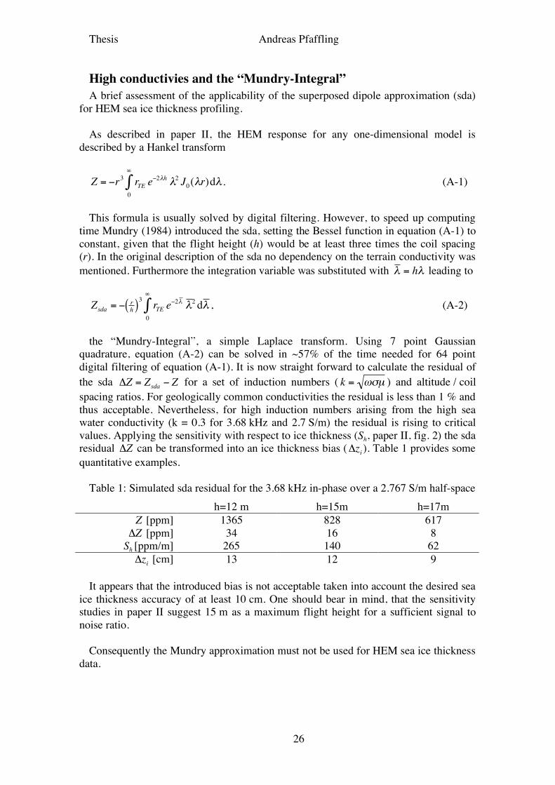
Thesis Andreas Pfaffling
26
High conductivies and the “Mundry-Integral” A brief assessment of the applicability of the superposed dipole approximation (sda)
for HEM sea ice thickness profiling. As described in paper II, the HEM response for any one-dimensional model is
described by a Hankel transform
!
Z = "r3 rTEe"2#h #2 J0(#r)
0
$
% d# . (A-1)
This formula is usually solved by digital filtering. However, to speed up computing
time Mundry (1984) introduced the sda, setting the Bessel function in equation (A-1) to constant, given that the flight height (h) would be at least three times the coil spacing (r). In the original description of the sda no dependency on the terrain conductivity was mentioned. Furthermore the integration variable was substituted with
!
" = h" leading to
!
Zsda
= " r
h( )3
rTEe"2# # 2
0
$
% d# , (A-2)
the “Mundry-Integral”, a simple Laplace transform. Using 7 point Gaussian
quadrature, equation (A-2) can be solved in ~57% of the time needed for 64 point digital filtering of equation (A-1). It is now straight forward to calculate the residual of the sda
!
"Z = Zsda# Z for a set of induction numbers (
!
k = "#µ ) and altitude / coil spacing ratios. For geologically common conductivities the residual is less than 1 % and thus acceptable. Nevertheless, for high induction numbers arising from the high sea water conductivity (k = 0.3 for 3.68 kHz and 2.7 S/m) the residual is rising to critical values. Applying the sensitivity with respect to ice thickness (Sh, paper II, fig. 2) the sda residual
!
"Z can be transformed into an ice thickness bias (
!
"zi). Table 1 provides some
quantitative examples. Table 1: Simulated sda residual for the 3.68 kHz in-phase over a 2.767 S/m half-space
h=12 m h=15m h=17m
!
Z [ppm] 1365 828 617
!
"Z [ppm] 34 16 8 Sh [ppm/m] 265 140 62
!
"zi [cm] 13 12 9
It appears that the introduced bias is not acceptable taken into account the desired sea
ice thickness accuracy of at least 10 cm. One should bear in mind, that the sensitivity studies in paper II suggest 15 m as a maximum flight height for a sufficient signal to noise ratio.
Consequently the Mundry approximation must not be used for HEM sea ice thickness
data.
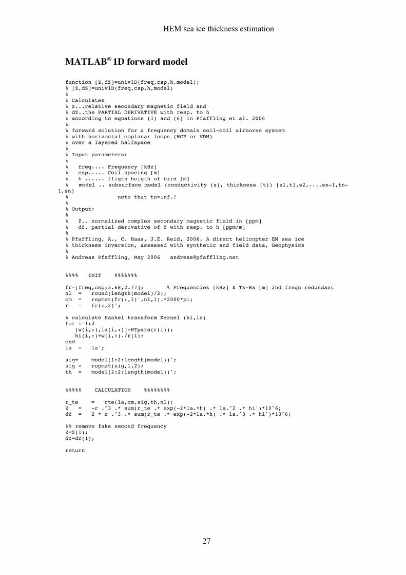
HEM sea ice thickness estimation
27
MATLAB® 1D forward model function [Z,dZ]=univ1D(freq,csp,h,model); % [Z,dZ]=univ1D(freq,csp,h,model) % % Calculates % Z...relative secondary magnetic field and % dZ..the PARTIAL DERIVATIVE with resp. to h % according to equations (1) and (6) in Pfaffling et al. 2006 % % forward solution for a frequency domain coil-coil airborne system % with horizontal coplanar loops (HCP or VDM) % over a layered halfspace % % Input parameters: % % freq.... Frequency [kHz] % csp..... Coil spacing [m] % h ...... fligth heigth of bird [m] % model .. subsurface model (conductivity (s), thickness (t)) [s1,t1,s2,...,sn-1,tn-
1,sn] % note that tn=inf.! % % Output: % % Z.. normalized complex secondary magnetic field in [ppm] % dZ. partial derivative of Z with resp. to h [ppm/m] % % Pfaffling, A., C. Haas, J.E. Reid, 2006, A direct helicopter EM sea ice % thickness inversion, assessed with synthetic and field data, Geophysics % % Andreas Pfaffling, May 2006 [email protected] %%%% INIT %%%%%%% fr=[freq,csp;3.68,2.77]; % Frequencies [kHz] & Tx-Rx [m] 2nd frequ redundant nl = round(length(model)/2); om = repmat(fr(:,1)',nl,1).*2000*pi; r = fr(:,2)'; % calculate Hankel transform Kernel (hi,la) for i=1:2 [w(i,:),la(i,:)]=HTpara(r(i)); hi(i,:)=w(i,:)./r(i); end la = la'; sig= model(1:2:length(model))'; sig = repmat(sig,1,2); th = model(2:2:length(model))'; %%%%% CALCULATION %%%%%%%% r_te = rte(la,om,sig,th,nl); Z = -r .^3 .* sum(r_te .* exp(-2*la.*h) .* la.^2 .* hi')*10^6; dZ = 2 * r .^3 .* sum(r_te .* exp(-2*la.*h) .* la.^3 .* hi')*10^6; %% remove fake second frequency Z=Z(1); dZ=dZ(1); return
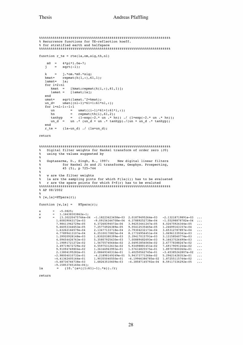
Thesis Andreas Pfaffling
28
%%%%%%%%%%%%%%%%%%%%%%%%%%%%%%%%%%%%%%%%%%%%%%%%%%%%%%%%%%%%%%%%%%% % Recurrence functions for TE-reflection koeff. % for stratified earth and halfspace %%%%%%%%%%%%%%%%%%%%%%%%%%%%%%%%%%%%%%%%%%%%%%%%%%%%%%%%%%%%%%%%%%% function r_te = rte(la,om,sig,th,nl) m0 = 4*pi*1.0e-7; j = sqrt(-1); k = j.*om.*m0.*sig; kmat= repmat(k(1,:),61,1); lamat= la; for i=2:nl kmat = [kmat;repmat(k(i,:),61,1)]; lamat = [lamat;la]; end umat= sqrt(lamat.^2+kmat); un_d= umat((nl-1)*61+1:61*nl,:); for i=nl-1:-1:1 un = umat((i-1)*61+1:61*i,:); hn = repmat(th(i),61,2); tanhyp = (1-exp(-2.* un .* hn)) ./ (1+exp(-2.* un .* hn)); un_d = un .* (un_d + un .* tanhyp)./(un + un_d .* tanhyp); end r_te = (la-un_d) ./ (la+un_d); return %%%%%%%%%%%%%%%%%%%%%%%%%%%%%%%%%%%%%%%%%%%%%%%%%%%%%%%%%%%%%%%%%%% % Digital filter weights for Hankel transform of order zero (J0) % using the values suggested by % % Guptasarma, D., Singh, B., 1997: New digital linear filters % for Hankel Jo and J1 transforms, Geophys. Prospecting, % 45 (5), p 725-744 % % w are the filter weights % la are the sampling pints for which F(la(i)) has to be evaluated % r are the space points for which f=f(r) has to be evaluted %%%%%%%%%%%%%%%%%%%%%%%%%%%%%%%%%%%%%%%%%%%%%%%%%%%%%%%%%%%%%%%%%%% % AP 08/2002 % % [w,la]=HTpara(r); function [w,la] = HTpara(r); a = -5.0825; s = 1.16638303862e-1; w = [3.30220475766e-04 -1.18223623458e-03 2.01879495264e-03 -2.13218719891e-03 ... 1.60839063172e-03 -9.09156346708e-04 4.37889252738e-04 -1.55298878782e-04 ... 7.98411962729e-05 4.37268394072e-06 3.94253441247e-05 4.02675924344e-05 ... 5.66053344653e-05 7.25774926389e-05 9.55412535465e-05 1.24699163157e-04 ... 1.63262166579e-04 2.13477133718e-04 2.79304232173e-04 3.65312787897e-04 ... 4.77899413107e-04 6.25100170825e-04 8.17726956451e-04 1.06961339341e-03 ... 1.39920928148e-03 1.83020380399e-03 2.39417015791e-03 3.13158560774e-03 ... 4.09654426763e-03 5.35807925630e-03 7.00889482693e-03 9.16637526490e-03 ... 1.19891721272e-02 1.56755740646e-02 2.04953856060e-02 2.67778388247e-02 ... 3.49719672729e-02 4.55975312615e-02 5.93498881451e-02 7.69179091244e-02 ... 9.91094769804e-02 1.26166963993e-01 1.57616825575e-01 1.89707800260e-01 ... 2.13804195282e-01 2.08669340316e-01 1.40250562745e-01 -3.65385242807e-02 ... -2.98004010732e-01 -4.21898149249e-01 5.94373771266e-02 5.29621428353e-01 ... -4.41362405166e-01 1.90355040550e-01 -6.19966386785e-02 1.87255115744e-02 ... -5.68736766738e-03 1.68263510609e-03 -4.38587145792e-04 8.59117336292e-05 ... -9.15853765160e-06]; la = (10.^(a+((1:61)-1).*s))./r; return
HEM sea ice thickness estimation
29
Bibliographic details of papers I-IV Paper I page: 31
Reid, J. E., Pfaffling, A., and Vrbancich, J. 2006. Airborne electromagnetic footprints in 1D earths, Geophysics, 71, G63-G72.
Published in March 2006 Paper II page: 43
Pfaffling, A., Haas, C., and Reid, J. E. 2006. A direct helicopter EM sea ice thickness inversion, assessed with synthetic and field data
Submitted in April 2006 to Geophysics, moderate revisions submitted October 2006, minor revision submitted January 2007, accepted February 2007.
Paper III page: 67
Pfaffling, A., and Reid, J. E. 2006. Sea ice as an evaluation target for HEM modeling and inversion
Submitted 08/2006 to Journal of Applied Geophysics. Paper IV page: 87
Reid, J. E., Pfaffling, A., Worby, A. P., and Bishop, J. R. 2006. In-situ measurements of the direct-current conductivity of Antarctic sea ice: implications for airborne electromagnetic sounding of sea ice thickness, Annals of Glaciology, 44, in press.
Submitted 10/2005 to Annals of Glaciology.

30

31
PAPER I

Paper I Reid, Pfaffling & Vrbancich
32
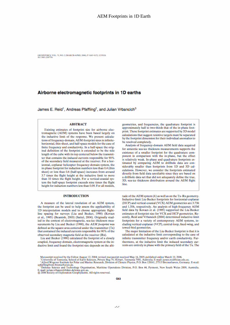
AEM Footprints in 1D Earth
33
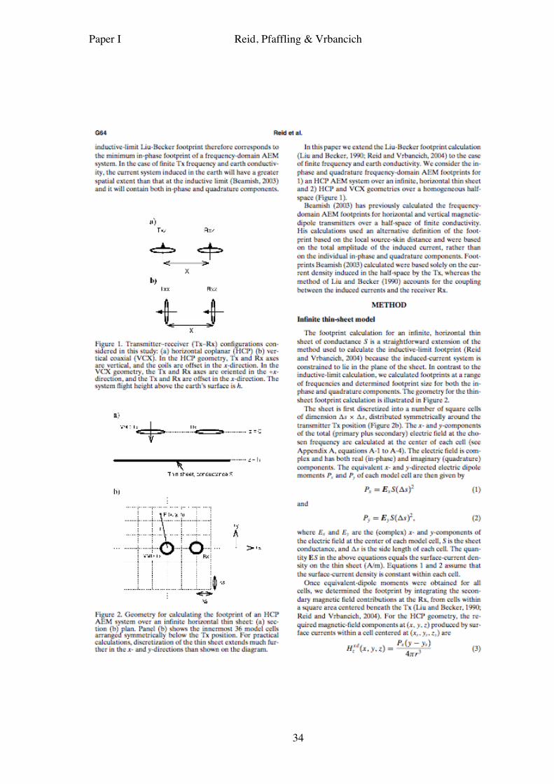
Paper I Reid, Pfaffling & Vrbancich
34
AEM Footprints in 1D Earth
35
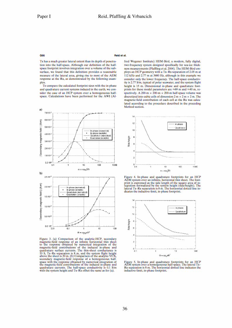
Paper I Reid, Pfaffling & Vrbancich
36
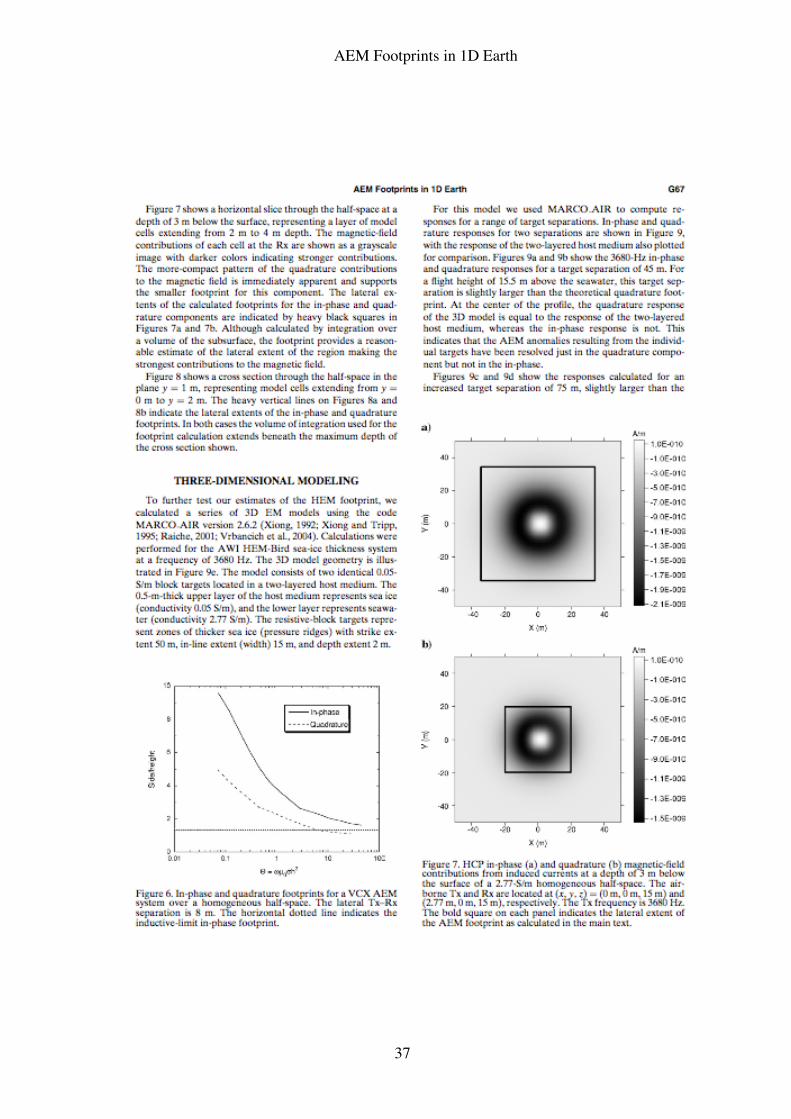
AEM Footprints in 1D Earth
37
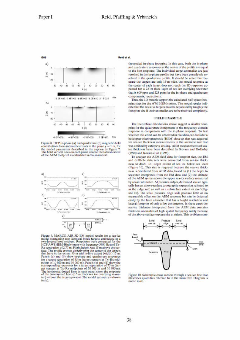
Paper I Reid, Pfaffling & Vrbancich
38
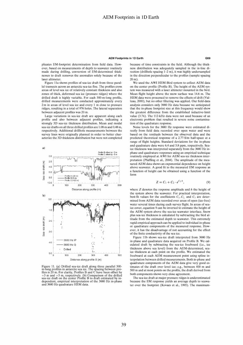
AEM Footprints in 1D Earth
39
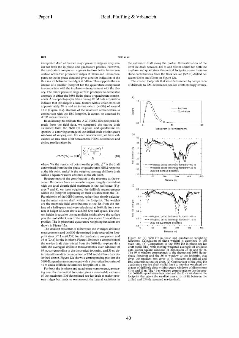
Paper I Reid, Pfaffling & Vrbancich
40
AEM Footprints in 1D Earth
41
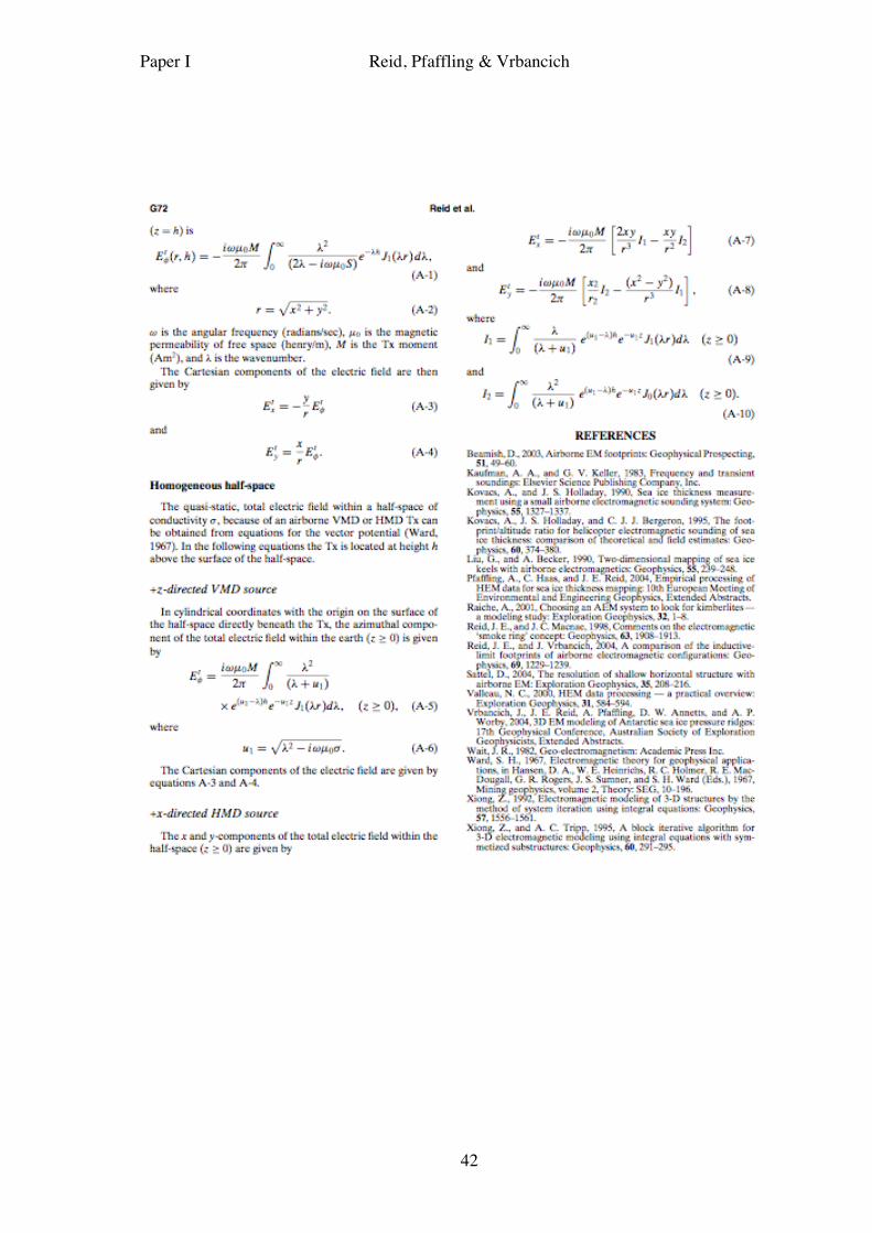
Paper I Reid, Pfaffling & Vrbancich
42

43
PAPER II

44
45
A DIRECT HELICOPTER EM - SEA ICE THICKNESS INVERSION, ASSESSED WITH SYNTHETIC AND FIELD DATA.
Andreas Pfaffling1
Christian Haas2
James E. Reid 3
1 formerly at Alfred Wegener Institute for Polar and Marine Research. Currently consulting geophysicist, Davidstr. 3, 20359 Hamburg, Germany. Email: [email protected], Ph: +49 179 6733979 2 Sea Ice Physics Section, Climate Sciences Research Division, Alfred Wegener Institute for Polar and Marine Research, P. O. Box 120161, 27515 Bremerhaven, Germany. Email: [email protected]
3 formerly at University of Tasmania, Hobart, Australia. Currently Geoforce Pty Ltd., 1/288 Victoria Rd., Malaga, 6090 WA, Australia. Email: [email protected]
Left-running header: Pfaffling, Haas and Reid Right-running header: Direct HEM sea ice thickness inversion
Manuscript submitted on April 12, 2006 Revised manuscript submitted on October 13, 2006 2nd Revised manuscript submitted on January 29, 2007 Paper accepted on February 23, 2007
Paper II Pfaffling, Haas & Reid
46
ABSTRACT Accuracy and precision of helicopter electromagnetic (HEM) sounding are the
essential parameters for HEM sea ice thickness profiling. For sea ice thickness research, the quality of HEM ice thickness estimates must be better than 10 cm to detect potential climatologic thickness changes. We introduce and assess a direct, one-dimensional HEM data inversion algorithm, resulting in sea ice thickness estimates. For synthetic quality assessment, an analytically determined HEM sea ice thickness sensitivity is used to derive precision and accuracy. Precision is directly related to random, instrumental noise, while accuracy is defined by systematic bias arising from the data processing algorithm. For the in-phase component of the HEM response, sensitivity increases with frequency and coil spacing but decreases with flying height. For small scale HEM instruments used in sea ice thickness surveys, instrumental noise must not exceed 5 ppm to reach ice thickness precision of 10 cm at 15 m nominal flying height. Comparable precision is yielded at 30 m height for conventional exploration HEM systems with bigger coil spacings. Accuracy losses due to approximations made for the direct inversion are negligible for brackish water and remain better than 10 cm for saline water. Synthetic precision and accuracy estimates are verified with drill hole validated field data from East Antarctica, where HEM derived level ice thickness agrees with drilling results to within 4 % or 2 cm.
INTRODUCTION As an indicator and a positively coupled variable of climate change, sea ice extent and
thickness distribution have been increasingly targeted in polar research over the last decade. The sea ice thickness distribution and ice extent in the Arctic and Antarctic Oceans is a key parameter in understanding the effects of global warming (ACIA, 2004). Besides passive microwave remote sensing data for sea ice extent (Stroeve et al., 2005), frequency domain electromagnetic induction has become widely used to study changes in the sea ice thickness distribution (Haas, 2004).
Regional mapping of the sea ice thickness distribution using helicopter electromagnetics (HEM) began in the late eighties in north America, and was further developed in Canada prior to the latest research in Europe since the mid 1990’s. Research on the applicability of helicopter EM for sea ice studies was initiated in 1985 by the U.S. Army Corps of Engineers’ Cold Regions Research and Engineering Laboratory (CRREL, Kovacs et al., 1987). During those first attempts, using a conventional four-frequency mineral exploration HEM system, ice thickness profiles were retrieved with reasonable accuracy. The overall results were promising enough to develop a sea ice dedicated, small scale, three-frequency sensor (Kovacs and Holladay 1990) and later a broadband system with frequencies up to 200 kHz (Kovacs et al., 1995). Similar development took place at the Bedford Institute of Oceanography (BIO) in Canada cooperating with the Canadian Coast Guard. Field tests started with a conventional exploration system (Holladay et al., 1990) leading to a small scale, two frequency towed instrument (Peterson et al., 1999) and most recently a four-frequency helicopter-nose hard mounted system (Prinsenberg et al., 2002).
The first European airborne EM sea ice field program was conducted in the Baltic sea using the Geological Survey of Finland’s (GSF) fixed wing EM system (Multala et al., 1996). After the reported campaigns in the winters ’91, ’93, and ’94, the GSF system has not been used for sea ice thickness surveys. The latest European development was initiated in 2000 by the Alfred Wegener Institute for Polar and Marine Research (AWI)
Direct HEM sea ice thickness inversion
47
in Bremerhaven, Germany. The AWI HEM system is a small scale, purpose built, adaptable, fully digital instrument which has been used on an operational basis during ship and land based expeditions in the Arctic, Antarctic and Baltic seas.
Distorted HEM data leads to difficulties with data processing resulting in inconsistencies between geophysical and ground truth data. Amongst further error sources, random instrumental noise degrades inversion results due to the high sensitivity of the commonly used least-squares inversion to outlying data points (Meju, 1994). Kovacs et al. (1987) mention a decrease in level ice thickness error from 19 % to 6 % by improving the inversion parameters. Experience gained since 1990 at BIO leads to operational, real time thickness inversion for their small scale sea ice profiler (Ice Probe, internal reports). As an alternative to elaborate integral inversion and to speed up and simplify inversion methods, Bergeron (1986) introduced a two-layer approximation of the analytic HEM response (modified image method, MIM). For a two frequency HEM system MIM converts in-phase and quadrature data directly to bird height, first layer thickness and conductivity as well as to the two layer conductivity contrast. This method has proofed successful for HEM bathymetry applications (Bergeron et al., 1989) and lately salinity mapping (Bryan et al., 2003). Besides of an analytical feasibility study (Bergeron et al., 1987) there is no evidence for operational usage of MIM for sea ice thickness mapping. For the sea ice case MIM appears to depend on an extremely high system frequency (6.5 MHz) to achieve a skin-depth smaller than the expected ice thickness.
Fundamentally simplifying sea ice thickness HEM inversion, we present a direct HEM data to ice thickness equation, termed the EMPEX transform (empirical exponential). The transform is based on a one-dimensional (1D) approximation of the sea ice thickness problem and a further exponential fit to layered earth HEM response curves. A detailed discussion on the performance of direct inversion (EMPEX transform) in comparison to a suite of least-squares layered earth inversion routines has been submitted to Journal of Applied Geophysics by Pfaffling and Reid. Here we concentrate on the definition and assessment of precision and accuracy of the EMPEX derived ice thickness estimates.
To provide a basic understanding of the theoretical precision and accuracy of sea ice thickness measurements made using the AWI-HEM system, we present an analytic sensitivity equation for the ice thickness case. Sensitivity is studied for the AWI geometry as well as conventional exploration HEM systems. The EMPEX transform is assessed with synthetic data for saline and brackish water conditions, simulating Arctic or Antarctic and Baltic or Caspian seas respectively. A field data example from an expedition to East Antarctica in 2003 (Massom et al., 2006) is presented to underline the EMPEX performance compared to ground truth data.
Paper II Pfaffling, Haas & Reid
48
INSTRUMENTATION – THE AWI HEM SYSTEM In contrast to commercially-available multi-frequency exploration HEM systems with
bird lengths between 8 to 10 m and weights of up to 300 kg, the AWI HEM system is a two frequency instrument housed in a 3.4 m long towed bird weighing slightly more than 100 kg. The AWI system utilizes two horizontal coplanar transmitter – receiver loop pairs operating at 3.68 kHz (f1) and 112 kHz (f2) with coil separations of 2.77 m and 2.05 m respectively. The bird is supplied with on board calibration coils allowing phase and gain checks during every base level drift ascent. Ascents to ~800 ft are performed every 20 flight minutes to adjust the zero level of the measured secondary electromagnetic field (Valleau, 2000). Drift controls in-between these drift ascents are frequently conducted, when open water patches are crossed during ice thickness profiling. Comparing those measurements with their respective half-space model response, guarantees sufficient drift linearity for post flight correction. Data acquisition and pre-processing is conducted by a PC inside the bird, sampling the EM data at 10 Hz and the built in laser altimeter at 100 Hz. The 20 m long towing cable solely connects to the helicopter’s 28 V DC outlet, allowing the system to be carried by a broad variety of helicopter types. A wireless network connection between the bird PC and the operator laptop in the aircraft allows in-flight bird control and data display. The system is usually flown at nominally 15 m height with 60 to 80 knots. A detailed description on the system and its technical specialties and performance will be given elsewhere (paper in preparation to be submitted to Journal of Applied Geophysics by Haas et al.). However, here we focus on the innovative processing method developed for the instrument.
METHODS The basic principle of HEM sea ice thickness profiling is to estimate the bird to water
distance from the EM data, while a laser altimeter in the bird determines the system height above the ice or snow surface. The difference between these two distances consequently corresponds to the ice (or ice + snow) thickness. Whenever sea ice thickness is mentioned in this paper, it actually refers to the total thickness meaning ice thickness plus snow thickness. There is no way to distinguish between snow and ice by HEM with the described system configuration. When interpreting electromagnetic data for sea ice thickness generally two different ice types have to be considered. The first and more complicated case is deformed ice, so called pressure ridges, where the ice floes have been broken up, crushed against each other and finally piled up into distinct topographic features. Attempts to process HEM data related to these 3D features were made at the University of California at Berkeley by Liu and Becker (1990). These involved a compilation of interpretation charts for common pressure ridge shapes. Eventually an elaborate 2D inversion scheme was presented (Liu et al., 1991). However, due to the necessary extensive and advanced computing and only minor improvements in field results, multi dimensional data processing is not yet used on an operational basis. Furthermore the geometry of real world pressure ridges is rarely as simple as presumed by the 2D models involved in the inversion. Being composed of a mixture of single, broken blocks of ice and ocean water, pressure ridges are very difficult to describe even by drill hole thickness measurements. Therefore ground truth data to validate processing algorithms can not be acquired with the desired accuracy and detail. Idealized structure models of pressure ridges are sketched in Kovacs and
Direct HEM sea ice thickness inversion
49
Holladay (1990, Figure 5) showing the high keel porosity. The underestimation of pressure ridge thickness due to 1D EM processing is discussed by Reid et al. (2003).
In contrast to deformed ice, most sea ice is composed of homogeneous level ice, representing a computationally-simpler 1D situation. Level ice thickness mainly depends on the thermodynamic growing conditions while pressure ridges are linked to short term events like storms. All approximations considered in this study focus on the determination of level ice thickness.
General HEM 1D forward modeling For a 1D subsurface geometry (layered half-space) the HEM response for the vertical
dipole mode can be expressed as a Hankel transform utilizing a Bessel function of the first kind of order zero (
!
J0) leading to
!
Z = "r3 rTEe"2#h #2 J0(#r)
0
$
% d# (1)
with r being the coil separation, h the receiver and transmitter height above ground and
!
" the wave number. The recursively determined transverse electric (TE) mode reflection coefficient
!
rTE
is a function of system frequency and the electromagnetic properties of the conducting half-space as given in Ward and Hohmann (1988).
!
Z is the normalized, secondary magnetic field at the receiver coil position usually expressed in ppm.
!
Z = Hz
SH
z
P , with
!
Hz
P being the primary (field in a non-conductive full-space) and
!
Hz
S the secondary magnetic field strength (field above a conductive half-space arising from the eddy currents induced by the primary field). For a homogeneous half-space
!
rTE
can be expressed as a straight forward quotient and hence the layered half-space solution, equation 1, simplifies to:
!
Z = "r3# " #2 + i$%µ
# + #2 + i$%µe"2#h #2 J0(#r)
0
&
' d# (2)
Here the kernel now includes the angular frequency of the EM field ( f!" 2= ) as well as the electrical conductivity
!
" , and magnetic permeability
!
µ of the conducting half-space. The appearance of the imaginary unit
!
i in the homogeneous half-space solution, equation 2, underlines the complex nature of Z, usually described as in-phase (IP) and quadrature (Q) component or channel. In this study the 1D models for layered and homogeneous half-space, as given in equation 1 and 2, are computed by means of digital filtering as described in Guptasarma and Singh (1997).
Electrical properties of sea ice covered oceans Saline ocean water and brackish seawater represent distinct sea ice environments, as
they exhibit different electromagnetic target characteristics. The Arctic Oceans and the Southern Ocean surrounding Antarctica are characterized by saline ocean water with salinities around 35 PSU (±5) while brackish water prevails in the northern Baltic (< 6 PSU) and Caspian Seas (10-13 PSU). The parameter of main interest is the conductivity of the water below the sea ice cover, which is a function of salinity and water temperature. In polar conditions and in the presence of sea ice the water temperature is commonly close to the freezing point resulting in electric conductivities of 2.4 S/m to 2.8 S/m for Arctic or Antarctic waters and ~0.3 S/m or ~1 S/m for Baltic or Caspian water.
Paper II Pfaffling, Haas & Reid
50
The conductivity of sea ice is generally about two magnitudes smaller than the water it was formed from, as most of the brine is expelled from the ice while it freezes. Bulk ice conductivities between 20 mS/m and 50 mS/m can be presumed for newly formed first year (FY) ice (Timco 1979). Once an ice floe survives one summer melt season, almost all of its remaining enclosed brine has been drained out and the conductivity decreases by another order of magnitude. Due to both the growth structure of sea ice where brine cells assume a preferred vertical orientation and the subsequent development of vertical brine channels, level ice shows a strong vertical-to-horizontal conductivity anisotropy with the horizontal conductivity smaller than the vertical (Thyssen et al., 1974). This makes it practically transparent for EM induction in contrast to the highly conductive ocean. Based on sea ice model studies, Morey et al. (1984) show that the bulk ice conductivity may not exceed 50 mS/m. Note that so far strictly bulk conductivity was addressed, which is not necessarily the parameter, picked up by EM induction. The in-situ conductivity of sea ice is hard to measure on samples, as the conductive brine drains out of the ice structure when an ice core is drilled and taken to a lab. However, recent in situ DC resistivity measurements in Antarctica (Reid et al., 2006b) indicate an even smaller horizontal conductivity than usually expected averaging at 17 mS/m.
For the synthetic HEM data presented in this paper seawater and sea ice conductivities of 2.767 S/m and 50 mS/m or 0.3 S/m and 1 mS/m were used for Ant-/Arctic (short for Antarctic and Arctic) or Baltic conditions respectively. For comparability with earlier studies, we decided to use 50 mS/m as Polar sea ice conductivity, rather than the actual lower values from in-situ measurements.
Approximations involved For HEM sea ice thickness mapping, the bird altitude over the conductive ocean
water is the model parameter of interest. To develop a direct inversion method, deriving the distance to water three main approximations are made:
1) Conductive seawater half-space The seawater conductivity is assumed to be known and constant. Though the water
salinity and consequently conductivity may change significantly on a regional scale, it can be assumed as constant within a certain survey area. As an example the measured sea water conductivity statistics along the track north of 80° latitude of an RV POLARSTERN expedition to the northern Fram Strait (Schauer and Kattner, 2004) result in an average of 2.713 S/m with 0.042 S/m standard deviation. Thermosalinometer data of RV AURORA AUSTRALIS (Massom et al., 2006) acquired in the East Antarctic result in an average sea water conductivity of 2.769 S/m with 0.054 S/m standard deviation. Significantly different sea water conductivities may exist in distinct oceanographic regions (e.g. Lincoln Sea 2.4 S/m, unpublished AWI field campaign). However, once the local water conductivity is determined, it is likely to be constant as long as there are no disturbing features such as river mouths or other oceanographic anomalies.
2) Resistive sea ice layer The sea ice conductivity is neglected, making the ice transparent to HEM induction.
Due to the pronounced contrast between the sea water and ice conductivity of two to three orders of magnitude and the small ice thickness compared to the bird height the majority of the induced eddy currents flow in the conductive seawater. Model studies
Direct HEM sea ice thickness inversion
51
comparing synthetic data for conductive and transparent ice are shown in the accuracy section, proving that for ice of moderate thickness (2-3 m) the effect of its conductivity is negligible for low frequencies.
3) Model dimensionality The sea ice structure is simplified to a 1D problem. As discussed before, being
interested in the thermodynamic history of the sea ice cover the level ice thickness is the key parameter. Obviously 2D and 3D features in the ice structure will be smoothed due to the 1D processing and the footprint size of the induction process (Reid et al., 2003). Lateral smoothing has a minor effect on ice thickness distribution function, which is used to determine regional level ice thickness and will be introduced in the EMPEX assessment section.
Limitations The vast majority of common situations in sea ice thickness mapping allow for the
use of the EMPEX approximations. However, rare or extreme sea ice conditions may exist, where the assumptions don’t hold and thus EMPEX may yield biased sea ice thickness estimates. One extreme condition met in late Antarctic summer is the development of gap layers - highly porous partially melted layers near the ice surface. Gap layers are highly conductive (close to sea water conductivity) and therefore bias direct inversion results towards underestimated thickness. A rarely met problem in Polar oceans is shallow water, which would rule out the approximation of the conductive seawater by a half-space. In the shallow northern Baltic Sea biased ice thickness are evident for water depths less than 10 m. Direct inversion can not account for bird attitude (roll & pitch) variations, which may have significant influence on the thickness estimates, mainly due to the tilted laser altimeter (Holladay et al., 1997). Layered earth inversion would be able to account for sea ice conductivity variations as well as shallow bathymetry, given a suitable set of frequencies and coil spacing. If bird attitude is measured, it can be included in the inversion procedure.
Towards a direct inversion Taking into account the introduced approximations in the half-space solution,
equation 2 simplifies to a function solely depending on the bird height h. Hence applying numerical integration (e.g. Newton-Cotes formulae, Abramowitz and Stegun, 1964, Section 25.4.) the Hankel transform can be approximated by a series of exponential functions
!
Z(h) " BieCih
i=0
n
# . (3)
Reducing the series to n=2 with
!
C0
= 0 leads to
!
Z(h) " B0
+ B1e#C1h + B
2e#C2h . (4)
Equation 4 is here called second order approximation (as n=2) to the layered half-space response, equation 2. The coefficients B0, B1 , B2 , C1, and C2 are determined by exponential fitting to synthetic half-space model curves within a given height range. Figure 1 illustrates the fitting quality and gives a comparison to the first order EMPEX approximation (
!
Z " B0
+ B1e#C
1h), which is commonly used for EM31 ice thickness
estimation (Haas et al., 1997). The exponential fit in Figure 1 is run for a 10 to 20 m flying height range.
Paper II Pfaffling, Haas & Reid
52
While the inverse of the first order approximation could be determined as an explicit logarithmic equation, the required model parameter h (the distance from bird to sea water surface) in the 2nd order approximation, equation 4, is evaluated with a root-finding algorithm using a Lagrange interpolation polynomial (Brent, 1973). Hence the distance between bird and water surface (
!
hEM
) can be determined for any measured EM field Z in an unambiguous, numerically robust way. The ice thickness is consequently derived by
!
zi= h
EM" h
L (5)
with
!
hL being the bird height measured by the laser altimeter and
!
zi the ice (total)
thickness.
Sensitivity In geophysical inversion the Jacobian matrix describes the system’s sensitivity
to specific model parameters, consisting of partial derivatives of measured data with respect to all model parameters. For a layered half-space HEM response, equation 1, the sensitivity (S) with respect to h, the parameter of interest in this case, can be expressed analytically. The partial derivative of Z with respect to h for a homogeneous half-space leads to equation 6, describing the HEM sensitivity to the bird height over ocean water.
!
S ="Z
"h= 2r3
# $ #2 + i%&µ
# + #2 + i%&µe$2#h #3 J0(#r)
0
'
( d# (6)
RESULTS The sensitivity, equation 6, provides the opportunity to theoretically study the utility
of HEM for sea ice thickness mapping. Two profoundly different data quality measures are described in this section, precision and accuracy. The former is governed by instrumental system noise, translated to precision estimates using determined sensitivity values. In contrast to the precision, residuals introduced by the mentioned EMPEX approximations relate to the method’s accuracy. Finally the EMPEX transform is used on synthetic data sets, to assess the quality of the determined sea ice thickness estimates. This leads to the final assessment of the method studying the superposition of the effects of limited precision due to system noise and decreasing accuracy caused by biases introduced by the approximations made.
Precision due to instrumental noise To investigate the theoretically achievable precision in sea ice thickness estimates,
sensitivity studies have been conducted for the major sea ice environments. Highly saline Arctic and Southern ocean water as well as brackish Baltic water was considered. Sensitivity was computed analytically (equation 6) at typical flying heights for small scale sea ice birds such as the AWI HEM system as well as conventional exploration birds.
Sensitivity and precision for a small bird In Climate Research the targeted ice thickness accuracy is 10 cm. Presuming a
instrumental noise level of 5 ppm, this leads to a sensitivity threshold of 50 ppm/m to meet the required precision. The dashed line in Figure 2 shows the 50 ppm/m threshold and consequently illustrates the maximum bird heights for the distinct channels. It
Direct HEM sea ice thickness inversion
53
further points out the necessity of small instrumental noise levels to keep the maximum flying height in a safe range for field operations.
Governed by the water conductivity the maximum sensitivity channel is the 3.68 kHz IP for Ant-/Arctic and 112 kHz IP for Baltic waters (Figure 2). Additionally to the half-space sensitivities a set of two layer cases were investigated towards sensitivity with respect to first layer thickness. Table 1 provides results for 18 m bird above water surface height. With a skin-depth significantly larger than the ice thickness, f1 is not affected by the conductivity of the thin ice layer. The two layer model results coincide with the half-space curve. In contrast to the validity of the half-space approximation for f1 IP & Q and even f2 IP, the conductive ice layer influences the high frequency quadrature. However, the 112 kHz Q sensitivity is well below the noise level even for the half-space model and therefore not recommendable for ice thickness retrieval.
Universal Sensitivities For a more detailed understanding and better comparability to common HEM
geometries, sensitivities as introduced before were determined for a broad frequency and coil spacing range. Compared to conventional exploration systems, the technical and geophysical challenge in sea ice thickness retrieval is the small bird size and low flying altitude. Analyzing the system sensitivities reveals some fundamental characteristics. Sensitivity was determined within a range of 100 Hz to 1 MHz system frequency and 0.5 m to 10 m coil spacing for Ant-/Arctic (Figure 3a) as well as Baltic (Figure 3b) conditions at sensor heights of 15 m and 30 m. The highest and lowest frequency (with respective coil spacing) for four HEM systems is spotlighted in the graphs. (1) For the AWI mini-bird, (2) one more small scale sea ice bird, BIO’S Ice Probe (Peterson et al., 1999), (3) the conventional exploration bird used by CRREL in 1985 (Kovacs et al., 1987) and (4) for Fugro Airborne Survey’s RESOLVE bird, a modern 6 frequency exploration system (Smith et al., 2003).
Extending the findings for the AWI geometry, the sensitivity is a function of frequency and coil spacing (r). The higher S for f1 IP compared to f2 IP in Figure 2a is actually due to the higher coil spacing rather than the lower frequency. The coil spacing dominates the in-phase sensitivity for frequencies above 10kHz. While the IP sensitivity generally increases steadily with f and r, the Q sensitivity peaks at a discrete frequency for given r. For f1 the very large coil spacing of the RESOLVE bird balances the higher operating altitude resulting in S comparable to the AWI bird at 15 m height for the lowest frequency (AWI ~140 ppm/m, RESOLVE ~120 ppm/m). The low frequency of the CRREL bird results in a sensitivity of ~80 ppm/m, which makes it less suitable for EMPEX processing. However, the lowest of the four CRREL frequencies was designed for successful sub-ice bathymetry mapping, which can be achieved using layered earth inversion. The comparably large footprint at h = 30 m (Reid et al., 2006a), may explain the unsatisfactory sea ice thickness results obtained with conventionally sized birds (Kovacs et al., 1987). Sensitivities for the vertical coplanar and vertical coaxial channels in the CRREL and RESOLVE bird were computed for comparison and were generally smaller than the horizontal coplanar channels with comparable coil spacing (not shown).
Paper II Pfaffling, Haas & Reid
54
The accuracy of an approximation Applying the determined sensitivities the bias due to treating sea ice as
electromagnetic transparent, the second approximation made for the EMPEX transform, can be quantified. Neglecting the sea ice conductivity introduces a residual (R [ppm]), which is used to express an EMPEX-transform accuracy (A) estimated by the quotient of R and S (
!
A = R S [m]). R is defined as the difference between the half-space and two layer solution determined using two models with equal distance to water as in Table 1. As an example, R for the Arctic is determined by R = Zh - Zi, with
!
Zh being the half-
space response at h = 15 m and
!
Zi the result for a two layer case with h = 12 m above
an 3 m thick, conductive (0.05 S/m) ice layer, both on a 2.767 S/m ocean. For accuracies shown in Figure 4, an ice thickness of 3 and 2 m was used for Ant-/Arctic and Baltic environments respectively.
As both R and S are mainly a function of r3 (besides the r in the Bessel function) the accuracy mainly depends on the frequency (equations 1 & 6). For the range of A in Figure 4, the difference in accuracy for 2 or 8 m coil spacing is less than 3 %, hence only 2 m results are shown here. The decrease of accuracy (increase in number means decrease in quality) with increasing frequency is mainly driven by the strongly rising residual towards higher frequency, while the sensitivity’s slope levels out for IP or even declines in the case of Q. The accuracy generally suffers from high bird altitude and cannot be improved by increased coil spacing as the sensitivity. To meet the respective 15 m accuracy at higher altitude, the frequency has to be decreased leading to lower sensitivity and consequently worse precision in addition to the larger footprint at high altitude.
Precision and accuracy reveal opposite correlations with system frequency as far as the in-phase component is concerned. For the quadrature however, an optimal frequency with maximum precision exists, while the algorithm accuracy decreases with frequency as for IP. Consequently finding the right geometry-frequency trade off turns out to be the main problem in sea ice geophysics. The quadrature precision seems useful for choosing an optimal system frequency. A strong Q sensitivity would provide EMPEX results with high lateral resolution due to the smaller footprint of Q compared to IP (Reid et al., 2006a). The system geometry is usually limited by operational aspects. A low flying system with a large transmitter-receiver separation would be favorable but rather challenging for engineers and pilots and operations on icebreakers. However, increasing the spacing of the AWI bird’s 3.68 kHz coils from 2.77 m to 3.5 m (like BIO’s IceProbe) would already roughly double the IP sensitivity.
Synthetic assessment of the EMPEX transform To study the discussed effects of accuracy and precision on the EMPEX method,
synthetic data were EMPEX transformed and are analyzed as follows. The EM response was modeled for a sinusoidally-varying flying height between 10 and 20 m over a 3 m thick ice layer floating on saline ocean water. Three different cases were studied: In case (I) the ice conductivity was set to zero, simulating the half-space approximation, then (II) conductive ice was included with 50 mS/m and finally (III) Gaussian noise was added to the fields obtained for case (II) with standard deviation 6.4, 5.8, 9.2, and 10 ppm for f1 IP, f1 Q, f2 IP, and f2 Q respectively, representing typical field conditions (taken from the flight introduced in the field data section). For clarity the model ice thickness was subtracted from the EMPEX results in Figure 5 (a), c) & d)), consequently showing the thickness residual. Case (I) reveals the numerical accuracy of
Direct HEM sea ice thickness inversion
55
the exponential curve fitting, lying in the cm-range (mean error 0.5 cm
!
± 2 cm). Though the precision of (II) is still as good as in (I), the neglected ice conductivity introduces a residual decreasing the accuracy, as concluded from the precision and accuracy analysis earlier (mean error -7 cm
!
± 2 cm). Although fairly thick and conductive ice is modeled, the accuracy is better than 10 cm for f1 IP. Finally the highly noisy data - passing the EMPEX transform unfiltered – introduces a vast scatter in the resulting ice thickness estimates, increasing with height, due to the decreasing sensitivity. While the accuracy doesn’t suffer from the noise, the precision is significantly degraded (mean error -6 cm
!
± 12 cm). To get a reliable quality assessment of the EMPEX processing scheme, the sea ice
thickness distribution or histogram is introduced. Especially when it comes to Cross-correlation with remote sensing data, it is of priority to obtain a level ice thickness estimate of regional value rather then highly resolved lateral thickness maps or profiles. Consequently the thickness histogram (probability density function) is derived by standard statistical methods from thickness data along a certain section of the flight path and the mode of the distribution describes the wanted level ice thickness. Further the open water fraction is represented in the 0 to 10 cm thickness class and the tail of the distribution characterizes the pressure ridge height and density. Here we focus on the mode of the distribution, ideally identifying the original 1D level ice thickness used for the forward modeling. Ice thickness histograms are commonly clustered into 10 cm bins, leading to the charts in Figure 5 b). For all three described model cases, the histograms peak at the correct thickness within a tolerance of 10 cm. The high noise added in case (III) broadens the distribution but does not bias the mode.
It needs to be stressed, that the presented modeled accuracy examples represent worst case conditions. It is highly unlikely to meet ice with horizontal conductivities of 50 mS/m and even more unlikely to meet ice 3 m thick with high conductivities.
Ant-/Arctic The EMPEX performance for increasing ice thickness was assessed with synthetic
data computed according to the model drafted in Figure 6. A total of 6000 measurements for ice thickness from zero to six meter with varying bird height were modeled incorporating Ant-/Arctic conductivity parameters with added Gaussian noise as in case (III) in Figure 5. The histograms calculated for the low frequency IP and Q (Figure 7) point out the higher accuracy of IP as suggested before (bias between distribution mode and model thickness), while the precision of IP and Q is comparable (width of the distribution peaks). Filtering the raw EM data with a 5 point running average prior to EMPEX transformation (Figure 7b) has no effect in the position of the mode (accuracy). The signal to noise ratio and precision in the histogram improves, however.
Baltic Synthetic data for Baltic conditions with ice thickness from zero to two meters
analyzed as for the Ant-/Arctic case result in comparable ice thickness distributions (not shown). As the sensitivity is smaller for the brackish water, the histograms are broader and the bias due to ice conductivity is sufficiently small (within 10 cm for 2 m thick ice). Following from the precision and accuracy chapters (Figure 2 + 4), for brackish water the high frequency IP provides the best signal to noise ratio in the histogram, roughly two times the peak of f1 IP.
Paper II Pfaffling, Haas & Reid
56
FIELD DATA In September-October 2003, an Australian-led international experiment dedicated to
sea ice remote sensing validation (Massom et al., 2006), took place onboard the icebreaker RV AURORA AUSTRALIS in the east Antarctic marginal sea ice zone. During a three-day long ice station almost one thousand drill hole ice thickness measurements were made on three parallel 500-meter long, 20 m spaced profiles, offering a unique data set for obtaining ground truth for airborne EM data. For optimum validation data, a level ice floe with a prominent pressure ridge was chosen for this experiment. Ice core analyses and DC-soundings (Reid et al., 2006b) showed that the internal sea ice structure was homogeneous, lacking any disturbing features like highly conductive surface or slush layers. HEM data was acquired along the central drill hole profile at an average bird altitude of 14.7 m (15.1 m over water surface) and an operational speed of 60 knots (30 m/s). To co-locate HEM and drill hole data GPS-readings were taken on the drifting ice floe at the moment of the bird over-passing start and end of the line.
EMPEX thickness estimates from raw and filtered (5 point running average as in Figure 7) HEM data agree with drilled thickness data particularly along the ~0.5 m thick level ice areas (Figure 8). Being fairly thin and moderately saline, the level ice introduces no residual affecting the accuracy of the EMPEX transform. The underestimated level ice thickness between 90 and 130 m appears to be a bird swing effect. The mean error from measurements solely over level ice is – 0.04 m
!
± 0.09 m and – 0.07 m
!
± 0.09 m for f1 IP and f1 Q respectively. As anticipated, the massive 3D pressure ridge is underestimated in thickness by 50 %
using the 1D processing method. Note the steeper slope of the quadrature thickness in the vicinity of the major pressure ridge at 300 - 400 m due to the smaller footprint of Q (36 m) compared to IP (69 m; Reid et al., 2006a). However, though being smaller than the footprint, the narrow ridge at 80 m is observable in the derived ice thickness. This is solely due to the ridge topography, profiled by the laser, rather than the EM induction process.
Finally, comparing ice thickness histograms from drilling data as well as IP and Q EMPEX estimates proves the accuracy and precision of the EMPEX method (Figure 10). Even at 2 cm bin size EMPEX and drilling histograms yield the same modal thickness. Filtering the raw EM data has a smaller effect on field data than on synthetic data, as instrumental and “glaciological” noise (e.g. the surface roughness picked up by the laser altimeter) interfere. The precision of the histogram (width of the distribution) does not improve from filtering. The distinct peak in the drilling histogram is widened up in the HEM results, just as predicted from the precision discussion earlier (Figures 5 & 7) as well as due to bird swing effects between 90 and 130 m as mentioned above.
Direct HEM sea ice thickness inversion
57
CONCLUSIONS A one-dimensional, approximate direct HEM inversion algorithm is described and
evaluated. We introduce an analytical definition for sensitivity with respect to sea ice thickness. This enables us to quantify precision and accuracy estimates for HEM ice thickness mapping. Biases due to approximations included in the described EMPEX processing algorithm define the systems accuracy. For generally expected sea ice conditions, EMPEX accuracy is within the usually desired 10 cm. Synthetic precision, governed by instrumental noise, is better than 10 cm given small noise levels (< 5 ppm) and sensor altitudes (~ 15 m) for small scale system geometries as used in sea ice HEM.
Besides these quantitative specifications, EMPEX ice thickness estimates may be degraded by three dimensional sea ice geometries, such as pressure ridges as well as rare phenomena as highly conductive gap layers within the ice floe or shallow water in the area of investigation. Formal layered earth inversion in contrast, could account for anomalous ice conductivities or bathymetric effects. Further biases due to bird swing could be avoided by inversion, while EMPEX would underestimate the ice thickness due to bird pitch and roll. Apart from the mentioned limitations, EMPEX appears to be the favourable processing scheme especially for the described AWI – HEM system for instrumental / technical reasons: The component chosen for EMPEX processing (3.68 kHz in-phase) is characterized by (a) the highest sensitivity with respect to ice thickness and (b) the lowest instrumental noise level. Incorporating any other component (e.g. using least-square inversion) would degrade the resulting ice thickness precision and accuracy.
The derived half-space sensitivities are a valuable measure for comparing the performance of HEM instruments. Utilizing sensitivity values, technical noise specifications in ppm can be transferred to model-space precision estimates in centimeters. The field data example confirms the synthetically stated precision estimates (12 cm) when studying the retrieved level ice thickness precision (9 cm).
If the EMPEX transform is applied on the full HEM dataset, a set of ice thickness estimates is computed. Generally these thicknesses should coincide, as along the level ice in Figure 8 for 3.68 kHz IP & Q. The consistency of distinct thickness estimates may act as an indicator of 3D features in the vicinity. Note, that on the flanks of the main pressure ridge in Figure 8, IP and Q diverge, due to the smaller footprint of Q compared to IP. The most dominant cause of occasional poor accuracy for EMPEX sea ice thickness, however, appears to be the unaccounted pitch and roll movements of the HEM bird. If attitude measurements would be available, attitude effects could be corrected transforming distorted EM fields to HMD fields and tilted laser altitudes to nadir measures. This way, attitude corrected data could be fed through the EMPEX transform, still avoiding elaborate layered earth inversion.
Our results confirm the EMPEX transform as a useful, very stable and fast tool for ground-, ship- and airborne EM sea ice thickness profiling.
Paper II Pfaffling, Haas & Reid
58
ACKNOWLEDGMENTS Parts of this research have been funded by the EC research project “SITHOS”. We
thank the ARISE 2003 shipboard party for conducting almost 1000 drill-hole measurements of sea ice thickness, the officers and crew of the RV AURORA AUSTRALIS for field support and the pilots and technicians of Helicopter Resources Pty Ltd. Insightful comments from three anonymous reviewers, the associate editor and the editor substantially improved the original manuscript.
REFERENCES Abramowitz, M., and I. A. Stegun, 1964, Handbook of Mathematical Functions with
Formulas, Graphs, and Mathematical Tables: Dover publications, ISBN 0-486-61272-4.
ACIA, 2004, Impacts of a Warming Arctic, Arctic Climate Impact Assessment: Cambridge University Press, ISBN 0521617782.
Bergeron. C. J., Jr., 1986, Modified image method: Application to the response of layered ohmic conductors to active electromagnetic sources: Journal of Applied Physics, 59, 3901-3908.
Bergeron, C. J., J. W. Ioup, and G. A. Michel, 1987, Lateral resolution of the modified image method for sea-ice thickness: 57th Annual International Meeting, SEG, Expanded Abstracts , Session:EM1.3.
Bergeron, C. J., J. W. Ioup, and G. A. Michel, 1989, Interpretation of airborne electromagnetic data using the modified image method: Geophysics, 54, 1023-1030.
Brent, R. P. 1973, Algorithms for Minimization Without Derivatives, in G. Forsythe, ed., Prentice-Hall Series in Automatic Computation: ISBN 0-13-022335-2.
Bryan, M. W., K. W. Holladay, C. J. Bergeron, J. W. Ioup, and G. E. Ioup, 2003, MIM and nonlinear least-squares inversions of AEM data in Varaataria basin, Louisiana: Geophysics, 68, 1126-1131.
Guptasarma, D., and B. Singh, 1997, New digital linear filters for Hankel J0 and J1 transforms: Geophysical Prospecting, 45, 745-762.
Haas, C., S. Gerland, H. Eicken, and H. Miller, 1997, Comparison of sea- ice thickness measurements under summer and winter conditions in the Arctic using a small electromagnetic induction device: Geophysics, 62, 749–757.
Haas, C. 2004, Late-Summer Sea Ice Thickness Variability in the Arctic Transpolar Drift 1991-2001 derived from ground-based Electromagnetic Sounding: Geophysical Research Letters, 31, L09402, doi:10.1029/2003GL019394.
Holladay, J. S., J. R. Rossiter, and A. Kovacs, 1990, Airborne measurements of sea-ice thickness using Electromagnetic induction sounding: 9th Conf. of Offshore Mechanics and Arctic Engineering, Conference Proceedings, 309-315.
Holladay, J. S., B. Lo, and S. J. Prinsenberg, 1997, Bird Orientation Effects in Quantitative Airborne Electromagnetic Interpretation of Pack Ice Thickness Sounding: Oceans Conference 1997, Marine Technology Society / Institute of Electrical and Electronics Engineers Inc., Conference Proceedings, Vol. 2, 1114-1119.
Kovacs, A., N. C. Valleau, and J. S. Holladay, 1987, Airborne electromagnetic sounding of sea-ice thickness and subice bathymetry: Cold Regions Science and Technology, 14, 289–311.
Kovacs, A. and J. S. Holladay, 1990, Sea ice thickness measurement using a small airborne electromagnetic sounding system: Geophysics, 55, 1327-1337.
Direct HEM sea ice thickness inversion
59
Kovacs, A., J. S. Holladay, and C. J. J. Bergeron, 1995, The footprint/altitude ratio for helicopter electromagnetic sounding of sea ice thickness: comparison of theoretical and field estimates: Geophysics, 60, 374–380.
Liu, G., and A. Becker, 1990, Two-dimensional mapping of sea ice keels with airborne electromagnetics: Geophysics, 55, 239-248.
Liu, G., A. Kovacs, and A. Becker, 1991, Inversion of airborne electromagnetic survey data for sea-ice keel shape: Geophysics, 56, 1986–1991.
Massom, R., A. P. Worby, V. Lytle, T. Markus, I. Allison, T. Scambos, H. Enomoto, K. Tateyama, T. Haran, J. Comiso, A. Pfaffling, T. Tamura, A. Muto, P. Kanagaratnam, B. Giles, N. Young, and G. Hyland, 2006, ARISE (Antarctic Remote Ice Sensing Experiment) in the East 2003: Validation of satellite-derived sea-ice data products: Annals of Glaciology, 44, in press
Meju, M., 1994, Geophysical data analysis: Understanding inverse problem theory and practice: Society of Exploration Geophysicists, ISBN 1-56080-027-5.
Morey, R.M., A. Kovacs, and G. F. N. Cox, 1984, Electromagnetic properties of sea ice: Cold Regions Science and Technology, 9, 53–75.
Multala, J., H. Hautaniemi, M. Oksama, M. Lepparanta, J. Haapala, A. Herlevi, K. Riska, and M. Lensu, 1996, An airborne system on a fixed-wing aircraft for sea ice thickness mapping: Cold Regions Science and Technology, 24, 355–373.
Peterson, I. K., S. J. Prinsenberg, and J. S. Holladay, 1999, Using a Helicopter-Borne EM-Induction System to Validate RADARSAT Sea Ice Signatures: 28th International Conference on Port and Ocean Engineering under Arctic Conditions (POAC), Conference Proceedings, Vol. 1, 275-284.
Prinsenberg, S. J., J. S. Holladay, and J. Lee, 2002, Measuring Ice Thickness with EISFlowTM, a Fixed-mounted Helicopter Electromagnetic-laser System: 12th International Offshore and Polar Engineering Conference, Conference Proceedings, Vol. 1, 737-740.
Reid, J. E., J. Vrbancich, and A. P. Worby, 2003, A comparison of shipborne and airborne electromagnetic methods for Antarctic sea ice thickness measurements: Exploration Geophysics, 34, 46-50.
Reid, J. E., A. Pfaffling, and J. Vrbancich, 2006a, Airborne electromagnetic footprints in 1D earths: Geophysics, 71, G63-G72.
Reid, J. E., A. Pfaffling, A. P. Worby, and J. R. Bishop, 2006b, In-situ measurements of the direct-current conductivity of Antarctic sea ice: implications for airborne electromagnetic sounding of sea ice thickness: Annals of Glaciology, 44, in press.
Schauer, U., and G. Kattner, 2004, The Expedition ARKTIS XIX/1 a,b and XIX/2 of the Research Vessel "POLARSTERN" in 2003: Reports on Polar and Marine Research, 481, Alfred Wegener Institute for Polar and Marine Research.
Smith, B. D., D. V. Smith, P. L. Hill, and V. F. Labson, 2003, Helicopter Electromagnetic and Magnetic Survey Data and Maps, Seco Creek Area, Medina and Uvalde Counties, Texas: U.S. Geological Survey, Open-File Report 03-226.
Stroeve, J., M. C. Serreze, F. Fetterer, T. Arbetter, W. Meier, J. Maslanik, and K. Knowles, 2005, Tracking the Arctic's shrinking ice cover; another extreme September sea ice minimum in 2004: Geophysical Research Letters, 32, L04501, doi:10.1029/2004GL021810.
Timco, G. W., 1979, An analysis of the in-situ resistivity of sea ice in terms of its microstructure: Journal of Glaciology, 22, 461-471.
Thyssen, F., H. Kohnen, M. V. Cowan, and G. W. Timco, 1974, DC resistivity measurements on the sea ice near Pond Inlet, N. W. T. (Baffin Island): Polarforschung, 44, 117-126.
Paper II Pfaffling, Haas & Reid
60
Valleau, N. C., 2000, HEM data processing – a practical overview: Exploration Geophysics, 31, 584-594.
Ward, S. H. and G. W. Hohmann, 1988, Electromagnetic theory for geophysical applications, in M. N. Nabighian, ed., Electromagnetic methods in applied geophysics, Vol. 1, Theory, 131-311: Society of Exploration Geophysicists, ISBN 1-56080-069-0.
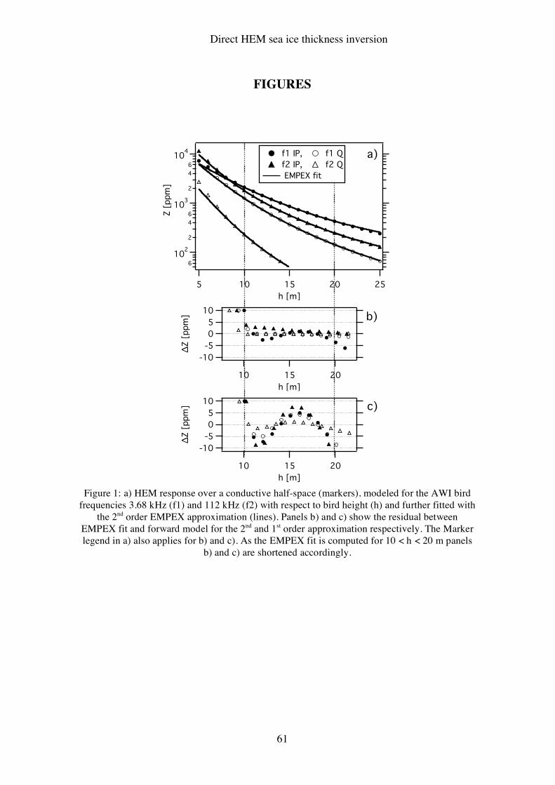
Direct HEM sea ice thickness inversion
61
FIGURES
6
102
2
4
6
103
2
4
6
104
Z [
ppm
]
252015105
h [m]
f1 IP, f1 Q
f2 IP, f2 Q
EMPEX fit
-10
-5
0
5
10
!Z [
ppm
]
201510
h [m]
-10
-5
0
5
10
!Z [
ppm
]
201510
h [m]
a)
b)
c)
Figure 1: a) HEM response over a conductive half-space (markers), modeled for the AWI bird
frequencies 3.68 kHz (f1) and 112 kHz (f2) with respect to bird height (h) and further fitted with the 2nd order EMPEX approximation (lines). Panels b) and c) show the residual between
EMPEX fit and forward model for the 2nd and 1st order approximation respectively. The Marker legend in a) also applies for b) and c). As the EMPEX fit is computed for 10 < h < 20 m panels
b) and c) are shortened accordingly.
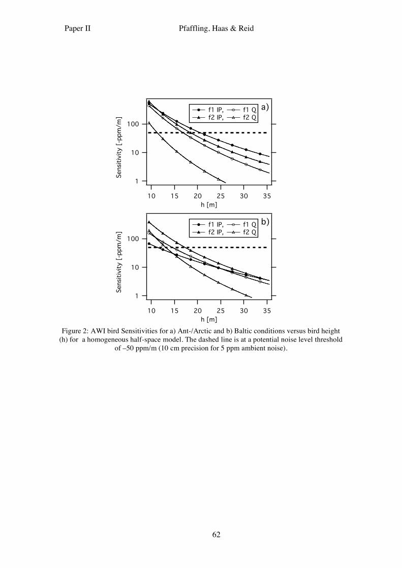
Paper II Pfaffling, Haas & Reid
62
1
10
100
Sensit
ivit
y [
-ppm
/m
]
353025201510
h [m]
b) f1 IP, f1 Q f2 IP, f2 Q
1
10
100Sensit
ivit
y [
-ppm
/m
]
353025201510
h [m]
a) f1 IP, f1 Q f2 IP, f2 Q
Figure 2: AWI bird Sensitivities for a) Ant-/Arctic and b) Baltic conditions versus bird height
(h) for a homogeneous half-space model. The dashed line is at a potential noise level threshold of –50 ppm/m (10 cm precision for 5 ppm ambient noise).
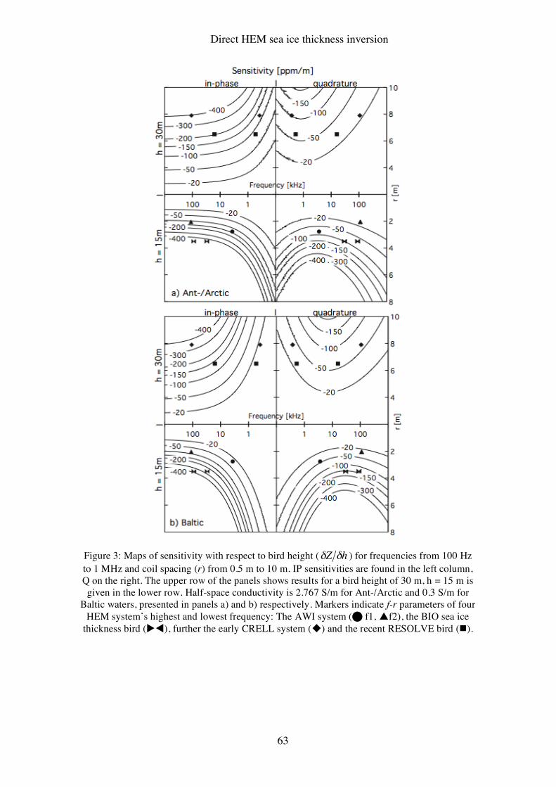
Direct HEM sea ice thickness inversion
63
Figure 3: Maps of sensitivity with respect to bird height (
!
"Z "h ) for frequencies from 100 Hz to 1 MHz and coil spacing (r) from 0.5 m to 10 m. IP sensitivities are found in the left column, Q on the right. The upper row of the panels shows results for a bird height of 30 m, h = 15 m is given in the lower row. Half-space conductivity is 2.767 S/m for Ant-/Arctic and 0.3 S/m for
Baltic waters, presented in panels a) and b) respectively. Markers indicate f-r parameters of four HEM system’s highest and lowest frequency: The AWI system ( f1, f2), the BIO sea ice
thickness bird (), further the early CRELL system () and the recent RESOLVE bird ().
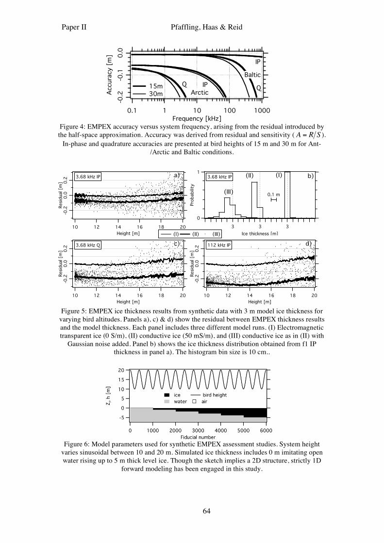
Paper II Pfaffling, Haas & Reid
64
-0.2
-0.1
0.0
Accura
cy [
m]
0.1 1 10 100 1000
Frequency [kHz]
15m 30m Arctic
Baltic
Q IPQ
IP
Figure 4: EMPEX accuracy versus system frequency, arising from the residual introduced by the half-space approximation. Accuracy was derived from residual and sensitivity (
!
A = R S ). In-phase and quadrature accuracies are presented at bird heights of 15 m and 30 m for Ant-
/Arctic and Baltic conditions.
-0.2
0.0
0.2
Resi
dual [m
]
201816141210
Height [m]
c)3.68 kHz Q
-0.2
0.0
0.2
Resi
dual [m
]
201816141210
Height [m]
a)3.68 kHz IP
-0.2
0.0
0.2
Resi
dual [m
]
201816141210
Height [m]
d)112 kHz IP
1
0
Pro
babili
ty
3 3 3
Ice thickness [m]
0.1 m
b)
(III)
(II) (I)3.68 kHz IP
(I) (II) (III)
Figure 5: EMPEX ice thickness results from synthetic data with 3 m model ice thickness for
varying bird altitudes. Panels a), c) & d) show the residual between EMPEX thickness results and the model thickness. Each panel includes three different model runs. (I) Electromagnetic transparent ice (0 S/m), (II) conductive ice (50 mS/m), and (III) conductive ice as in (II) with
Gaussian noise added. Panel b) shows the ice thickness distribution obtained from f1 IP thickness in panel a). The histogram bin size is 10 cm..
Figure 6: Model parameters used for synthetic EMPEX assessment studies. System height
varies sinusoidal between 10 and 20 m. Simulated ice thickness includes 0 m imitating open water rising up to 5 m thick level ice. Though the sketch implies a 2D structure, strictly 1D
forward modeling has been engaged in this study.
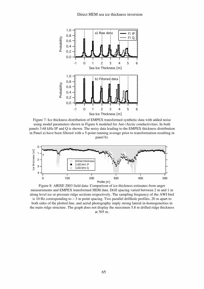
Direct HEM sea ice thickness inversion
65
1.0
0.8
0.6
0.4
0.2
0.0Pro
babili
ty6543210-1
Sea Ice Thickness [m]
f1 IP
f1 Q
a) Raw data
1.0
0.8
0.6
0.4
0.2
0.0
Pro
babili
ty
6543210-1
Sea Ice Thickness [m]
b) Filtered data
Figure 7: Ice thickness distribution of EMPEX transformed synthetic data with added noise using model parameters shown in Figure 6 modeled for Ant-/Arctic conductivities. In both
panels 3.68 kHz IP and Q is shown. The noisy data leading to the EMPEX thickness distribution in Panel a) have been filtered with a 5-point running average prior to transformation resulting in
panel b).
Figure 8: ARISE 2003 field data: Comparison of ice thickness estimates from auger
measurements and EMPEX transformed HEM data. Drill spacing varied between 2 m and 1 m along level ice or pressure ridge sections respectively. The sampling frequency of the AWI bird
is 10 Hz corresponding to ~ 3 m point spacing. Two parallel drillhole profiles, 20 m apart to both sides of the plotted line, and aerial photography imply strong lateral in-homogeneities in
the main ridge structure. The graph does not display the maximum 5.8 m drilled ridge thickness at 305 m.
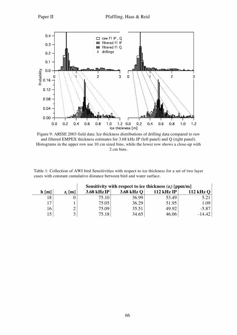
Paper II Pfaffling, Haas & Reid
66
Figure 9: ARISE 2003 field data: Ice thickness distributions of drilling data compared to raw
and filtered EMPEX thickness estimates for 3.68 kHz IP (left panel) and Q (right panel). Histograms in the upper row use 10 cm sized bins, while the lower row shows a close-up with
2 cm bins.
Table 1: Collection of AWI bird Sensitivities with respect to ice thickness for a set of two layer cases with constant cumulative distance between bird and water surface.
Sensitivity with respect to ice thickness (zi) [ppm/m] h [m] zi [m] 3.68 kHz IP 3.68 kHz Q 112 kHz IP 112 kHz Q
18 0 75.10 36.99 53.49 5.21 17 1 75.05 36.29 51.95 1.09 16 2 75.09 35.51 49.92 -5.87 15 3 75.18 34.65 46.06 -14.42

67
PAPER III

68
69
Sea Ice as an evaluation target for HEM modeling and inversion
Andreas Pfaffling a , b , ∗ James E. Reid c,d
a formerly at Sea Ice Physics Section, Climate Sciences Research Division, Alfred Wegener Institute for Polar and Marine Research, P. O. Box 120161, 27515 Bremerhaven, Germany. b recently Consulting Geophysicist, Eilbeker Weg 36, 22089 Hamburg, Germany, email: [email protected] c formerly at School of Earth Sciences, Private Bag 79, University of Tasmania, Hobart, Tasmania, 7001, Australia. d currently Geoforce Pty Ltd., 1/288 Victoria Rd., Malaga, 6090 WA, Australia, email: [email protected]
Manuscript uploaded to Journal of Applied Geophysics in August 06 standing by, waiting for the call for papers for the special issue on Airborne Geophysics. Submitted on January 31st 2007.
∗ Corresponding author. Ph: +49 179 6733979
Paper III Pfaffling and Reid
70
ABSTRACT We compare direct helicopter electromagnetic (HEM) data inversion for sea ice
thickness retrieval with three different formal, least squares layered earth inversion algorithms. For the two-frequency HEM system investigated, strongly variable sensitivities amongst the frequencies yields unstable inversion results. Layered earth inversion of, noisy synthetic data provides consistent sea ice conductivity for ice thicker than 3 m. Furthermore, formal inversion successfully accounts for partially melted, conductive sea ice layers and is able to determine shallow, sub – ice bathymetry in brackish water. Three - dimensional synthetic data introduces elevated sea ice conductivity artifacts in the layered earth inversion results. For a field data set of rather thin (~0.5 m) Antarctic sea ice, direct inversion prevails over the results from formal inversion. To ensure best data quality for inversion we introduce phasor diagram-based post flight system phase angle re-calibration. We suggest, that for the HEM system studied here, inversion fails due to the highly variable sensitivity of high and low frequency data components, the respective noise levels and the low sensitivity to sea ice conductivity especially for thin ice.
KEYWORDS
Helicopter electromagnetics, inversion, modelling, calibration, sea ice, Antarctica
INTRODUCTION Faced with global warming and the limited understanding of its processes and effects,
sea ice thickness distribution and extent has become a crucial parameter in climate research. The initial work on helicopter electromagnetic (HEM) regional sea ice thickness mapping was performed in the US and Canada in the early eighties (Kovacs et al., 1987; Holladay et al., 1990). Further European experiments in Finland and Germany followed up the reported American success (Multala et al., 1996; Haas et al., 2002) leading to an operational usage of HEM for sea ice thickness mapping in Arctic, Antarctic and Baltic waters. Furthermore, sea ice represents a useful target to validate the HEM method and commonly used processing algorithms. Unlike most geological targets, sea ice thickness can be ground truthed in high resolution with easily-drilled borehole measurements. Level sea ice, being undisturbed by dynamical processes and therefore flat, represents a one dimensional two layer model with a sharp boundary and well-established conductivities.
For the purpose built, two frequency HEM system operated by the Alfred Wegener Institute for Polar and Marine Research (AWI) a unique direct inversion approach (Pfaffling et al. 2006) is used as a rapid and non-ambiguous HEM data to sea ice thickness transform. In contrast to this transform, which relies on a number of assumptions and approximations, formal geophysical inversion may have a number of advantages. If inversion were able to yield reliable sea ice conductivity estimates, the salinity and therefore age of the ice could be determined. Further, the ice conductivity could act as a proxy for sea ice mechanical strength (Kovacs, 1996), a useful parameter in planning of polar shipping operations. Highly conductive inclusions in the ice sheet, as in gap layers or slush layers or pressure ridge keels could be detected by inverted conductivities, while they affect direct inversion results negatively. Finally when mapping sea ice on shallow water, bathymetry could be accounted for by inversion. Alternatively to finding more model parameters from the distinct data set, the accuracy
Sea ice to validate inversion algorithms
71
of the ice thickness itself, presuming all other parameters as known, might improve by full inversion of all HEM components.
The application of formal geophysical inversion to HEM data acquired over ice-covered waters was mentioned by Kovacs et al. (1987) and was successful in recovering shallow sub ice bathymetry. Kovacs and Holladay (1990) attempted to determine sea ice conductivity via layered-earth inversion, but generally considered the conductivity to be unreliable due to instrument drift and noise. Apart from a contractor report by Holladay et al. (1998) we are not aware of any peer reviewed paper, presenting validated sea ice conductivity inversion results from airborne electromagnetic data.
In this study we determine synthetic sea ice conductivity sensitivities for layered half-space models. Further we discuss inversion results for synthetic data for basic sea ice two layer models, a gap layer model and a Baltic Sea model including shallow bathymetry. Direct inversion is compared to three different least-squares inversion approaches. Furthermore three dimensional synthetic data is layered-earth inverted to study pressure ridge keel conductivity effects. Finally a field data example is discussed, comparing the different inversion algorithms and introducing a system phase re-calibration technique.
METHODS When HEM is applied for sea ice thickness mapping, small scale, purpose built
frequency-domain systems are generally used (Kovacs and Holladay, 1990; Haas et al., 2002). Systems are equipped with a laser altimeter in the towed “bird”, which also contains the induction coils. Consequently the distance between bird and ice or snow surface is well known and EM induction is utilized to determine the distance to the highly conductive water surface. The difference between these two distances yields the snow plus ice thickness, also called total thickness. The conductivity difference between the snow and ice layer can not be resolved by EM induction.
In contrast to deformed ice, most sea ice is composed of homogeneous level ice, representing a computationally-simpler one-dimensional (1D) situation. Level ice thickness mainly depends on the thermodynamic growing conditions while deformed sea ice at pressure ridges is related to short term events like storms. Most of the discussion in this study focuses on the determination of level ice thickness.
We applied four different inversion algorithms on synthetic 1D and 3D data. The principles used are briefly outlined in the following.
One dimensional forward modelling
For layered earth forward modeling we follow the standard theory given in Ward and Hohmann (1988). For a 1D subsurface, and subject to the quasi-static approximation, the HEM response for the vertical dipole mode (= horizontal coplanar, HCP) is expressed as a Hankel transform utilizing a Bessel function of the first kind of order zero (
!
J0) leading to
!
Z = "r3 rTEe"2#h #2 J0(#r)
0
$
% d# (1)
with r being the coil separation, h the receiver and transmitter height above ground and
!
" the wave number. The Hankel integral is calculated by digital filtering as described in Guptasarma and Singh (1997). The recursively determined transverse
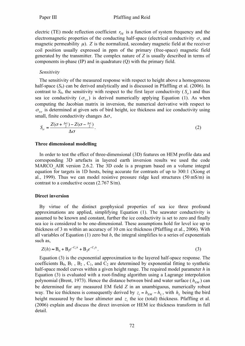
Paper III Pfaffling and Reid
72
electric (TE) mode reflection coefficient
!
rTE
is a function of system frequency and the electromagnetic properties of the conducting half-space (electrical conductivity
!
" , and magnetic permeability
!
µ).
!
Z is the normalized, secondary magnetic field at the receiver coil position usually expressed in ppm of the primary (free-space) magnetic field generated by the transmitter. The complex nature of Z is usually described in terms of components in-phase (IP) and in quadrature (Q) with the primary field.
Sensitivity The sensitivity of the measured response with respect to height above a homogeneous
half-space (Sh) can be derived analytically and is discussed in Pfaffling et al. (2006). In contrast to Sh, the sensitivity with respect to the first layer conductivity (
!
S" ) and thus sea ice conductivity (
!
"ice
) is derived numerically applying Equation (1). As when computing the Jacobian matrix in inversion, the numerical derivative with respect to
!
"ice
is determined at given sets of bird height, ice thickness and ice conductivity using small, finite conductivity changes
!
"# ,
!
S" =Z(" + #"
2) $ Z(" $ #"
2)
#". (2)
Three dimensional modelling
In order to test the effect of three-dimensional (3D) features on HEM profile data and corresponding 3D artefacts in layered earth inversion results we used the code MARCO_AIR version 2.6.2. The 3D code is a program based on a volume integral equation for targets in 1D hosts, being accurate for contrasts of up to 300:1 (Xiong et al., 1999). Thus we can model resistive pressure ridge keel structures (50 mS/m) in contrast to a conductive ocean (2.767 S/m).
Direct inversion
By virtue of the distinct geophysical properties of sea ice three profound approximations are applied, simplifying Equation (1). The seawater conductivity is assumed to be known and constant, further the ice conductivity is set to zero and finally sea ice is considered to be one-dimensional. These assumptions hold for level ice up to thickness of 3 m within an accuracy of 10 cm ice thickness (Pfaffling et al., 2006). With all variables of Equation (1) zero but h, the integral simplifies to a series of exponentials such as,
!
Z(h) " B0
+ B1e#C1h + B
2e#C2h . (3)
Equation (3) is the exponential approximation to the layered half-space response. The coefficients B0, B1 , B2 , C1, and C2 are determined by exponential fitting to synthetic half-space model curves within a given height range. The required model parameter h in Equation (3) is evaluated with a root-finding algorithm using a Lagrange interpolation polynomial (Brent, 1973). Hence the distance between bird and water surface (
!
hEM
) can be determined for any measured EM field Z in an unambiguous, numerically robust way. The ice thickness is consequently derived by
!
zi= h
EM" h
L, with
!
hL being the bird
height measured by the laser altimeter and
!
zi the ice (total) thickness. Pfaffling et al.
(2006) explain and discuss the direct inversion or HEM ice thickness transform in full detail.
Sea ice to validate inversion algorithms
73
Layered earth inversion
Least-squares layered earth inversion (LEI) was conducted using the freeware Gauss-Marquardt-Levenberg nonlinear parameter estimation package PEST by Watermark Numerical Computing (Doherty, 2003). In the standard 1D inversion, HEM data were generally inverted assuming a two-layered model with the sea ice thickness and conductivity allowed to vary, and the seawater conductivity fixed.
Conductance deficit
Due to the inherent nonuniqueness of EM inversion (Parker, 1977), overestimated LEI sea ice conductivity leads to underestimated ice thickness and vice versa. Biased LEI sea ice thickness can be avoided by post-processing the final model parameters from LEI using the ‘conductance deficit’ (CD) method. The CD method relies on the fact that cumulative conductance is the most stable parameter which can be recovered from LEI of EM data (Fullagar and Oldenburg, 1984). As previously described, the seawater conductivity (σsw) is always accurately known in HEM sea ice thickness surveys, and can be considered to be constant to the depth of penetration of the HEM system. If no sea ice were present, then the cumulative conductance (CC) to depth z metres within the seawater would be simply
!
CC = z"sw
. In cases where sea ice is present, then the cumulative conductance calculated to the same depth z from the final LEI model (CCLEI) will be less than
!
z"sw
. The quantity
!
CD = CC "CCLEI is the
conductance deficit. In practice, z must be chosen to be greater than the maximum sea ice thickness likely to be encountered in a given HEM survey area (z = 15 m allows a considerable safety margin for Antarctic sea ice studies). Because the sea ice conductivity (
!
"ice
< 0.05 S/m) is always much less than the seawater conductivity (σsw
!
" 2.7 S/m), we have
!
CD = ("sw#"
ice)z
i$"
swzi. The sea ice thickness can then be
estimated simply as
!
zi= CD "
sw
“Step by Step” (SbS) inversion
Being a two frequency system, the AWI bird’s measurements have different sensitivities to the sea ice thickness and ice conductivity. The low frequency (3.68 kHz) response is hardly affected by changes in the conductivity of the sea ice, and is controlled by the seawater conductivity. The high frequency (112 kHz) data is however more sensitive to the sea ice conductivity (see section 3.1.). Consequently a “step by step” (SbS) inversion approach was applied to the data. In the first step only the low frequency IP is considered to determine the ice thickness. For this stage of the inversion, the sea ice conductivity is fixed at zero. The second step in the algorithm is to fix the final, inverted thickness from the first step and invert the high frequency IP response for ice conductivity. Both steps are done using the PEST package as described above (section 2.4.). The SbS inversion is ought to result in more stable conductivity estimates than the simultaneous 1D inversion, especially in areas of thicker ice.
Paper III Pfaffling and Reid
74
RESULTS To investigate the ice conductivity resolvability from HEM data we first discuss the
numerical sensitivity of the EM field components with respect to ice thickness and conductivity. The theoretical performance of formal geophysical inversion is tested with synthetic data arising from a variety of 1D models. Finally 3D model data is fed into 1D inversion, revealing 3D artefacts in the 1D inversion results.
All synthetic studies are tuned to the geometry of the AWI sea ice HEM system. It comprises a two frequency, HCP towed bird, transmitting at 3.68 kHz and 112 kHz at a coil spacing of 2.77 m and 2.049 m respectively. A detailed description of the system is provided in Haas et al. (2002) and Pfaffling et al. (2006).
Sensitivity to ice conductivity
Sensitivity studies have been performed for sea ice conditions, typical for polar waters met in the Arctic Ocean or of the Antarctic coast. Brackish water of the northern Baltic Sea was neglected, as the conductivity of sea ice there is too low to have an effect on the HEM response (Pfaffling et al., 2006). The sea ice conductivity - sensitivity (
!
S" ) was computed for a layered earth model, consisting of a sea ice layer with conductivity 10 mS/m or 50 mS/m above a conductive half-space with 2.767 S/m (ocean water). Note that the used conductivities are conservative estimates, for conformity with earlier studies. Detailed in-situ DC resistivity studies (Thyssen et al., 1974; Reid et al., 2006a), describe a strong vertical / horizontal conductivity anisotropy, resulting in small conductivities in the horizontal plane. Sensitivity was determined for a nominal flying height of 15 m either for varying ice thickness (Figure 1a) or sea ice conductivity (Figure 1b). The difference in sensitivity between low and high system frequency is dramatic. While the low frequency is rather sensitive towards the ice thickness it is hardly affected by its conductivity and vice versa (Table 1). However, the sensitivity estimates are close to the noise level in both cases considering the desired accuracy in thickness or conductivity. In table 1 sensitivities are scaled in respect to desired accuracy quantities. Sea ice thickness must be estimated with less then 10 cm error, leading to the 3.68 kHz IP component with maximum thickness - sensitivity of ~9 ppm/(10cm), taken from Pfaffling et al. (2006). The expected sea ice conductivity change between first year (FY) and second- or multi year (MY) ice is within tens of mS/m, with values around 1 mS/m for MY and up to 60 mS/m for FY ice. Hence the 112 kHz Q component represents the highest sensitivity of ~12 ppm/(50mS/m) towards sea ice conductivity. The remaining components have sensitivities below the standard deviation (SD) of field data noise levels.
Inversion of 1D synthetic data
A suite of synthetic datasets were inverted using standard layered earth inversion including all four components of the AWI HEM system. Gaussian noise with standard deviations as in table 1 was added to the synthetic data. EM fields were computed at 15 m receiver and transmitter height for three different subsurface models.
To understand the basic resolvability of ice thickness and conductivity a set of two layer models consisting of sea ice (0.05 S/m) and sea water (2.767 S/m) with ice thickness from 0 to 5 m was inverted (Figure 2). Up to ice thickness of 3 m the sensitivity towards the ice conductivity is too small to determine stable inversion results
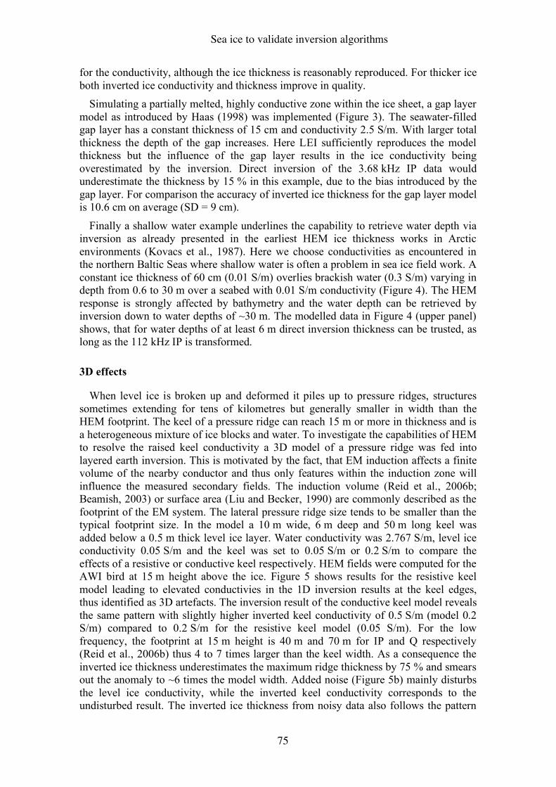
Sea ice to validate inversion algorithms
75
for the conductivity, although the ice thickness is reasonably reproduced. For thicker ice both inverted ice conductivity and thickness improve in quality.
Simulating a partially melted, highly conductive zone within the ice sheet, a gap layer model as introduced by Haas (1998) was implemented (Figure 3). The seawater-filled gap layer has a constant thickness of 15 cm and conductivity 2.5 S/m. With larger total thickness the depth of the gap increases. Here LEI sufficiently reproduces the model thickness but the influence of the gap layer results in the ice conductivity being overestimated by the inversion. Direct inversion of the 3.68 kHz IP data would underestimate the thickness by 15 % in this example, due to the bias introduced by the gap layer. For comparison the accuracy of inverted ice thickness for the gap layer model is 10.6 cm on average (SD = 9 cm).
Finally a shallow water example underlines the capability to retrieve water depth via inversion as already presented in the earliest HEM ice thickness works in Arctic environments (Kovacs et al., 1987). Here we choose conductivities as encountered in the northern Baltic Seas where shallow water is often a problem in sea ice field work. A constant ice thickness of 60 cm (0.01 S/m) overlies brackish water (0.3 S/m) varying in depth from 0.6 to 30 m over a seabed with 0.01 S/m conductivity (Figure 4). The HEM response is strongly affected by bathymetry and the water depth can be retrieved by inversion down to water depths of ~30 m. The modelled data in Figure 4 (upper panel) shows, that for water depths of at least 6 m direct inversion thickness can be trusted, as long as the 112 kHz IP is transformed.
3D effects
When level ice is broken up and deformed it piles up to pressure ridges, structures sometimes extending for tens of kilometres but generally smaller in width than the HEM footprint. The keel of a pressure ridge can reach 15 m or more in thickness and is a heterogeneous mixture of ice blocks and water. To investigate the capabilities of HEM to resolve the raised keel conductivity a 3D model of a pressure ridge was fed into layered earth inversion. This is motivated by the fact, that EM induction affects a finite volume of the nearby conductor and thus only features within the induction zone will influence the measured secondary fields. The induction volume (Reid et al., 2006b; Beamish, 2003) or surface area (Liu and Becker, 1990) are commonly described as the footprint of the EM system. The lateral pressure ridge size tends to be smaller than the typical footprint size. In the model a 10 m wide, 6 m deep and 50 m long keel was added below a 0.5 m thick level ice layer. Water conductivity was 2.767 S/m, level ice conductivity 0.05 S/m and the keel was set to 0.05 S/m or 0.2 S/m to compare the effects of a resistive or conductive keel respectively. HEM fields were computed for the AWI bird at 15 m height above the ice. Figure 5 shows results for the resistive keel model leading to elevated conductivies in the 1D inversion results at the keel edges, thus identified as 3D artefacts. The inversion result of the conductive keel model reveals the same pattern with slightly higher inverted keel conductivity of 0.5 S/m (model 0.2 S/m) compared to 0.2 S/m for the resistive keel model (0.05 S/m). For the low frequency, the footprint at 15 m height is 40 m and 70 m for IP and Q respectively (Reid et al., 2006b) thus 4 to 7 times larger than the keel width. As a consequence the inverted ice thickness underestimates the maximum ridge thickness by 75 % and smears out the anomaly to ~6 times the model width. Added noise (Figure 5b) mainly disturbs the level ice conductivity, while the inverted keel conductivity corresponds to the undisturbed result. The inverted ice thickness from noisy data also follows the pattern
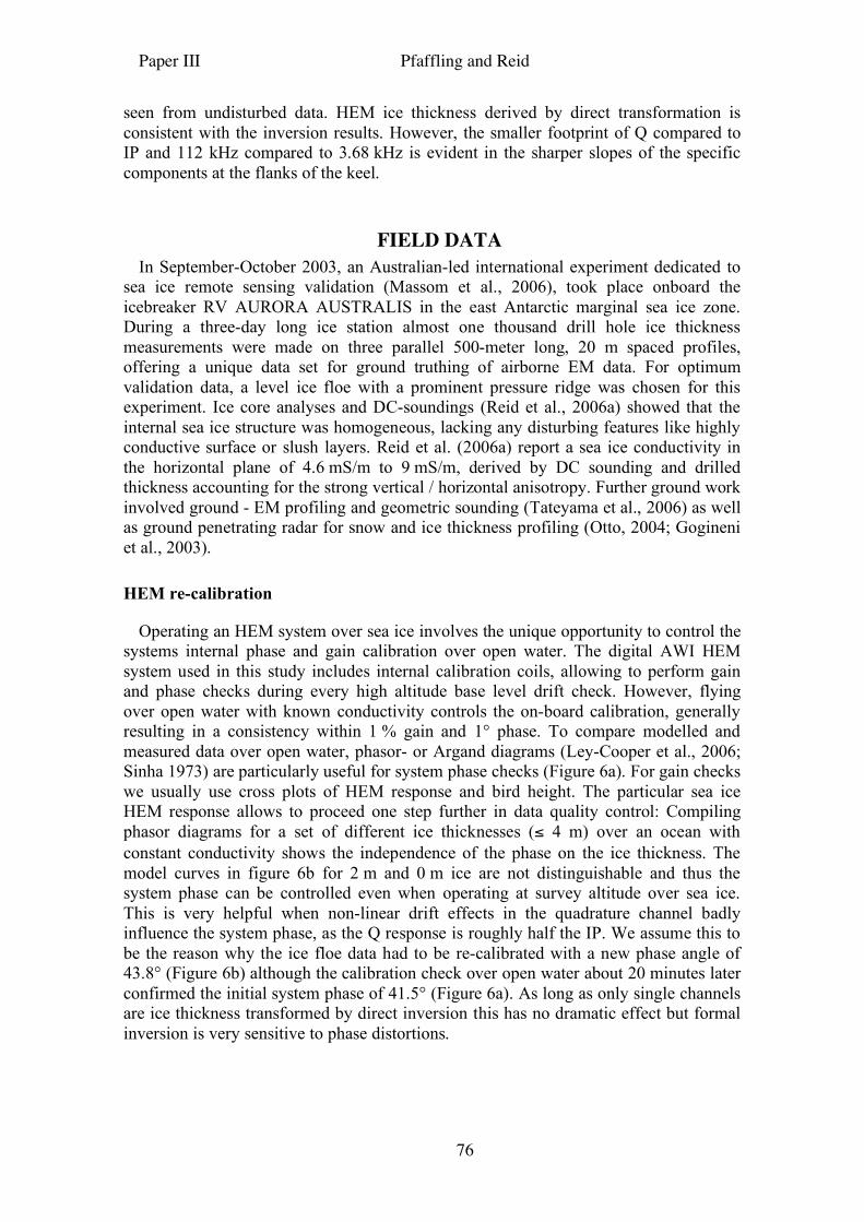
Paper III Pfaffling and Reid
76
seen from undisturbed data. HEM ice thickness derived by direct transformation is consistent with the inversion results. However, the smaller footprint of Q compared to IP and 112 kHz compared to 3.68 kHz is evident in the sharper slopes of the specific components at the flanks of the keel.
FIELD DATA In September-October 2003, an Australian-led international experiment dedicated to
sea ice remote sensing validation (Massom et al., 2006), took place onboard the icebreaker RV AURORA AUSTRALIS in the east Antarctic marginal sea ice zone. During a three-day long ice station almost one thousand drill hole ice thickness measurements were made on three parallel 500-meter long, 20 m spaced profiles, offering a unique data set for ground truthing of airborne EM data. For optimum validation data, a level ice floe with a prominent pressure ridge was chosen for this experiment. Ice core analyses and DC-soundings (Reid et al., 2006a) showed that the internal sea ice structure was homogeneous, lacking any disturbing features like highly conductive surface or slush layers. Reid et al. (2006a) report a sea ice conductivity in the horizontal plane of 4.6 mS/m to 9 mS/m, derived by DC sounding and drilled thickness accounting for the strong vertical / horizontal anisotropy. Further ground work involved ground - EM profiling and geometric sounding (Tateyama et al., 2006) as well as ground penetrating radar for snow and ice thickness profiling (Otto, 2004; Gogineni et al., 2003).
HEM re-calibration
Operating an HEM system over sea ice involves the unique opportunity to control the systems internal phase and gain calibration over open water. The digital AWI HEM system used in this study includes internal calibration coils, allowing to perform gain and phase checks during every high altitude base level drift check. However, flying over open water with known conductivity controls the on-board calibration, generally resulting in a consistency within 1 % gain and 1° phase. To compare modelled and measured data over open water, phasor- or Argand diagrams (Ley-Cooper et al., 2006; Sinha 1973) are particularly useful for system phase checks (Figure 6a). For gain checks we usually use cross plots of HEM response and bird height. The particular sea ice HEM response allows to proceed one step further in data quality control: Compiling phasor diagrams for a set of different ice thicknesses (≤ 4 m) over an ocean with constant conductivity shows the independence of the phase on the ice thickness. The model curves in figure 6b for 2 m and 0 m ice are not distinguishable and thus the system phase can be controlled even when operating at survey altitude over sea ice. This is very helpful when non-linear drift effects in the quadrature channel badly influence the system phase, as the Q response is roughly half the IP. We assume this to be the reason why the ice floe data had to be re-calibrated with a new phase angle of 43.8° (Figure 6b) although the calibration check over open water about 20 minutes later confirmed the initial system phase of 41.5° (Figure 6a). As long as only single channels are ice thickness transformed by direct inversion this has no dramatic effect but formal inversion is very sensitive to phase distortions.
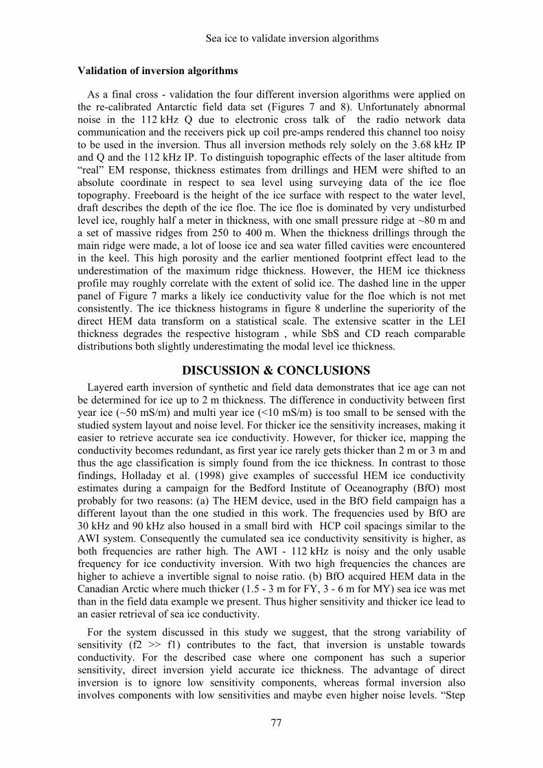
Sea ice to validate inversion algorithms
77
Validation of inversion algorithms
As a final cross - validation the four different inversion algorithms were applied on the re-calibrated Antarctic field data set (Figures 7 and 8). Unfortunately abnormal noise in the 112 kHz Q due to electronic cross talk of the radio network data communication and the receivers pick up coil pre-amps rendered this channel too noisy to be used in the inversion. Thus all inversion methods rely solely on the 3.68 kHz IP and Q and the 112 kHz IP. To distinguish topographic effects of the laser altitude from “real” EM response, thickness estimates from drillings and HEM were shifted to an absolute coordinate in respect to sea level using surveying data of the ice floe topography. Freeboard is the height of the ice surface with respect to the water level, draft describes the depth of the ice floe. The ice floe is dominated by very undisturbed level ice, roughly half a meter in thickness, with one small pressure ridge at ~80 m and a set of massive ridges from 250 to 400 m. When the thickness drillings through the main ridge were made, a lot of loose ice and sea water filled cavities were encountered in the keel. This high porosity and the earlier mentioned footprint effect lead to the underestimation of the maximum ridge thickness. However, the HEM ice thickness profile may roughly correlate with the extent of solid ice. The dashed line in the upper panel of Figure 7 marks a likely ice conductivity value for the floe which is not met consistently. The ice thickness histograms in figure 8 underline the superiority of the direct HEM data transform on a statistical scale. The extensive scatter in the LEI thickness degrades the respective histogram , while SbS and CD reach comparable distributions both slightly underestimating the modal level ice thickness.
DISCUSSION & CONCLUSIONS Layered earth inversion of synthetic and field data demonstrates that ice age can not
be determined for ice up to 2 m thickness. The difference in conductivity between first year ice (~50 mS/m) and multi year ice (<10 mS/m) is too small to be sensed with the studied system layout and noise level. For thicker ice the sensitivity increases, making it easier to retrieve accurate sea ice conductivity. However, for thicker ice, mapping the conductivity becomes redundant, as first year ice rarely gets thicker than 2 m or 3 m and thus the age classification is simply found from the ice thickness. In contrast to those findings, Holladay et al. (1998) give examples of successful HEM ice conductivity estimates during a campaign for the Bedford Institute of Oceanography (BfO) most probably for two reasons: (a) The HEM device, used in the BfO field campaign has a different layout than the one studied in this work. The frequencies used by BfO are 30 kHz and 90 kHz also housed in a small bird with HCP coil spacings similar to the AWI system. Consequently the cumulated sea ice conductivity sensitivity is higher, as both frequencies are rather high. The AWI - 112 kHz is noisy and the only usable frequency for ice conductivity inversion. With two high frequencies the chances are higher to achieve a invertible signal to noise ratio. (b) BfO acquired HEM data in the Canadian Arctic where much thicker (1.5 - 3 m for FY, 3 - 6 m for MY) sea ice was met than in the field data example we present. Thus higher sensitivity and thicker ice lead to an easier retrieval of sea ice conductivity.
For the system discussed in this study we suggest, that the strong variability of sensitivity (f2 >> f1) contributes to the fact, that inversion is unstable towards conductivity. For the described case where one component has such a superior sensitivity, direct inversion yield accurate ice thickness. The advantage of direct inversion is to ignore low sensitivity components, whereas formal inversion also involves components with low sensitivities and maybe even higher noise levels. “Step
Paper III Pfaffling and Reid
78
by Step” inversion shows that even when two channels (3.68 kHz IP + Q) are inverted to one model parameter, results don’t improve. This disproves one of the stated hypotheses, that inversion may yield more accurate thickness estimates. This, however, is a very specific result most likely not transferable to other system geometries and noise characteristics.
The 3D shape of pressure ridge introduce a conductivity artefact in 1D inversion, which can not be distinguished from the effect of a really conductive keel. This is especially unfortunate, as further insight into the inner pressure ridge structure would be of great interest. Lately DC resistivity tomography was performed on Arctic and Baltic pressure ridges with the aim to get a higher resolved geophysical image of the keel (Flinspach, 2005). Models retrieved via 3D inversion of the DC resistivity data are highly complex and publication of the results is in preparation.
However, inversion is capable to determine sea ice thickness if internal gap layers or shallow water are encountered, cases where direct inversion thickness is biased, as the assumed approximations are invalid.
Phasor diagrams are an important tool for data quality control of the system’s calibration phase angle. As the influence of ice thickness is hardly visible in phasor plots, modelled half-space response curves can be used for phase checks of field data at the target, rather than only over open water. This opens an excellent chance for further calibration checks in combination to open water control flight segments and internal calibration coils.
A substantial remaining problem is bird attitude (pitch, roll) which has an observable effect on HEM ice thickness estimates. Measured pitch and roll angles could be included into inversion and consequently eliminated in the thickness results. Besides from gap layers and bathymetry, the correction of bird attitude could be inversion’s most dominant impact on HEM ice thickness quality improvement. Bird pitch and roll biases the retrieved ice thickness in two ways. The altitude measured by the laser is biased as the laser looks at an angle rather than at nadir. Furthermore the EM induction process is distorted as the receiver and transmitter coils change in orientation and position. Quantitative analytic studies for the sea ice case are not available today, but we suggest that the biased laser height might have the strongest influence.
ACKNOWLEDGMENTS Parts of this work were supported by the Antarctic Climate & Ecosystems
Cooperative Research Centre (ACE CRC) based in Hobart / Australia within the AWI – ACE CRC exchange program, and by Australian Antarctic Science (AAS) grant #2381. The conductance deficit approach was suggested to JER by Dr Niels Bøie Christensen of the University of Aarhus. We thank the ARISE 2003 shipboard party for conducting almost 1000 drill-hole measurements of sea ice thickness, the officers and crew of the RV AURORA AUSTRALIS for field support and the pilots and technicians of Helicopter Resources Pty Ltd.
REFERENCES Beamish, D., 2003. Airborne EM footprints. Geophysical Prospecting 51, 49–60. Brent, R. P., 1973. Algorithms for Minimization Without Derivatives. in G. Forsythe,
ed., Prentice-Hall Series in Automatic Computation: ISBN 0-13-022335-2. Doherty, J., 2003. Groundwater model calibration using Pilot Points and Regularisation.
Ground Water 41 (2), 170-177.
Sea ice to validate inversion algorithms
79
Flinspach, D., 2005. Gleichstromgeoelektrik zur Erkundung der inneren Struktur und der Dicke von Meereis. Masters thesis (in German), Ludwig-Maximilians-Universität München, Germany.
Fullagar, P. K., and D. W. Oldenburg, 1984. Inversion of horizontal loop electromagnetic frequency soundings. Geophysics 49, 150-164.
Gogineni, S, K. Wong, S. Krishnan, P. Kanagaratnam, T. Markus, and V. Lytle., 2003. An ultra-wideband radar for measurements of snow thickness over sea ice. Proc. Int. Geosc. Rem. Sens. Symp., IGARSS ’03, 4, 2802-2804.
Guptasarma, D., and B. Singh, 1997. New digital linear filters for Hankel J0 and J1 transforms. Geophysical Prospecting 45, 745-762.
Haas, C., 1998. Evaluation of ship-based electromagnetic-inductive thickness measurements of summer sea-ice in the Bellingshausen and Amundsen Seas, Antarctica. Cold Regions Sci. Technol. 27, 1-16.
Haas C., Edeler H., Schürmann M., Lobach J. and Sengpiel K.-P., 2002. First operation of AWI HEM-bird for sea-ice thickness sounding. 62. Jahrestagung der Deutschen Geophysikalischen Gesellschaft DGG, Hannover, Germany, Conference Proceedings, 36-38.
Holladay, J. S., J. R. Rossiter, and A. Kovacs, 1990. Airborne measurements of sea-ice thickness using Electromagnetic induction sounding. 9th Conf. of Offshore Mechanics and Arctic Engineering, Conference Proceedings, 309-315.
Holladay, J.S., R.Z. Moucha and S.J. Prinsenberg, 1998. Airborne Electromagnetic Sea Ice Sounding Measurements During SIMMS’95. Canadian Contractor Report of Hydrography and Ocean Sciences 50: vii +179.
Kovacs, A., 1996. Estimating the full-scale tensile, flexural and compressive strength of first-year ice. Cold Regions Research and Engineering Laboratory Report 96-11.
Kovacs, A. and J. S. Holladay, 1990. Sea ice thickness measurement using a small airborne electromagnetic sounding system. Geophysics 55, 1327-1337.
Kovacs, A., N. C. Valleau, and J. S. Holladay, 1987. Airborne electromagnetic sounding of sea-ice thickness and subice bathymetry. Cold Regions Science and Technology 14, 289–311.
Ley-Cooper, Y., J. Macnae, T. Robb, and J. Vrbancich, 2006. Identification of calibration errors in helicopter electromagnetic (HEM) data through transform to the altitude-corrected phase-amplitude domain. Geophysics 71, G27-G34.
Liu, G., and A. Becker, 1990. Two-dimensional mapping of sea ice keels with airborne electromagnetics. Geophysics 55, 239–248.
Massom, R., A. P. Worby, V. Lytle, T. Markus, I. Allison, T. Scambos, H. Enomoto, K. Tateyama, T. Haran, J. Comiso, A. Pfaffling, T. Tamura, A. Muto, P. Kanagaratnam, B. Giles, N. Young, and G. Hyland, 2006. ARISE (Antarctic Remote Ice Sensing Experiment) in the East 2003: Validation of satellite-derived sea-ice data products. Annals of Glaciology 44, in press.
Multala, J., H. Hautaniemi, M. Oksama, M. Lepparanta, J. Haapala, A. Herlevi, K. Riska, and M. Lensu, 1996. An airborne system on a fixed-wing aircraft for sea ice thickness mapping. Cold Regions Science and Technology 24, 355–373.
Otto, D., 2004. Validierung von Bodenradar-Messungen der Eis- und Schneedicke auf ein- und mehrjährigem Meereis in Arktis und Antarktis. Masters thesis (in German), Technical University Clausthal, Germany.
Parker, R. L., 1977. Understanding inverse theory. Annual Review of Earth and Planetary Sciences, 5, 35-64.
Pfaffling, A., Haas, C., and Reid, J. E., 2006. A direct helicopter EM sea ice thickness inversion, assessed with synthetic and field data. Geophysics in press.
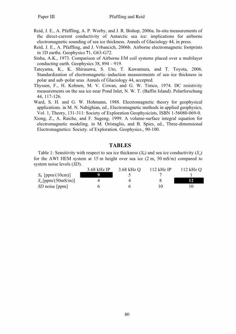
Paper III Pfaffling and Reid
80
Reid, J. E., A. Pfaffling, A. P. Worby, and J. R. Bishop, 2006a. In-situ measurements of the direct-current conductivity of Antarctic sea ice: implications for airborne electromagnetic sounding of sea ice thickness. Annals of Glaciology 44, in press.
Reid, J. E., A. Pfaffling, and J. Vrbancich, 2006b. Airborne electromagnetic footprints in 1D earths. Geophysics 71, G63-G72.
Sinha, A.K., 1973. Comparison of Airborne EM coil systems placed over a multilayer conducting earth. Geophysics 38, 894 – 919.
Tateyama, K., K. Shirasawa, S. Uto, T. Kawamura, and T. Toyota, 2006. Standardization of electromagnetic–induction measurements of sea–ice thickness in polar and sub–polar seas. Annals of Glaciology 44, accepted.
Thyssen, F., H. Kohnen, M. V. Cowan, and G. W. Timco, 1974. DC resistivity measurements on the sea ice near Pond Inlet, N. W. T. (Baffin Island). Polarforschung 44, 117-126.
Ward, S. H. and G. W. Hohmann, 1988. Electromagnetic theory for geophysical applications. in M. N. Nabighian, ed., Electromagnetic methods in applied geophysics, Vol. 1, Theory, 131-311: Society of Exploration Geophysicists, ISBN 1-56080-069-0.
Xiong, Z., A. Raiche, and F. Sugeng, 1999. A volume-surface integral equation for electromagnetic modeling. in M. Oristaglio, and B. Spies, ed., Three-dimensional Electromagnetics: Society. of Exploration. Geophysics., 90-100.
TABLES Table 1: Sensitivity with respect to sea ice thickness (Sh) and sea ice conductivity (Sσ)
for the AWI HEM system at 15 m height over sea ice (2 m, 50 mS/m) compared to system noise levels (SD).
3.68 kHz IP 3.68 kHz Q 112 kHz IP 112 kHz Q Sh [ppm/(10cm)] 9 5 7 1 Sσ [ppm/(50mS/m)] 4 4 8 12 SD noise [ppm] 6 6 10 10
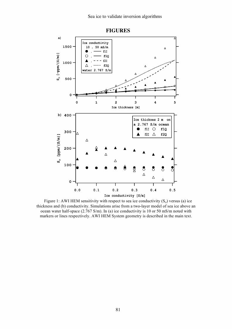
Sea ice to validate inversion algorithms
81
FIGURES
Figure 1: AWI HEM sensitivity with respect to sea ice conductivity (Sσ) versus (a) ice
thickness and (b) conductivity. Simulations arise from a two-layer model of sea ice above an ocean water half-space (2.767 S/m). In (a) ice conductivity is 10 or 50 mS/m noted with markers or lines respectively. AWI HEM System geometry is described in the main text.
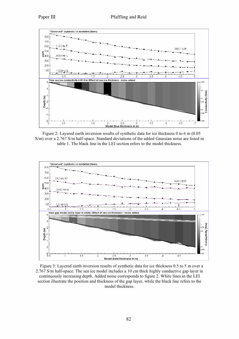
Paper III Pfaffling and Reid
82
Figure 2: Layered earth inversion results of synthetic data for ice thickness 0 to 6 m (0.05
S/m) over a 2.767 S/m half-space. Standard deviations of the added Gaussian noise are listed in table 1. The black line in the LEI section refers to the model thickness.
Figure 3: Layered earth inversion results of synthetic data for ice thickness 0.5 to 5 m over a
2.767 S/m half-space. The sea ice model includes a 10 cm thick highly conductive gap layer in continuously increasing depth. Added noise corresponds to figure 2. White lines in the LEI
section illustrate the position and thickness of the gap layer, while the black line refers to the model thickness.
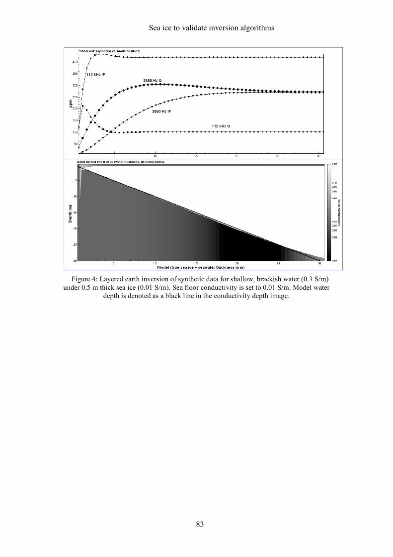
Sea ice to validate inversion algorithms
83
Figure 4: Layered earth inversion of synthetic data for shallow, brackish water (0.3 S/m)
under 0.5 m thick sea ice (0.01 S/m). Sea floor conductivity is set to 0.01 S/m. Model water depth is denoted as a black line in the conductivity depth image.
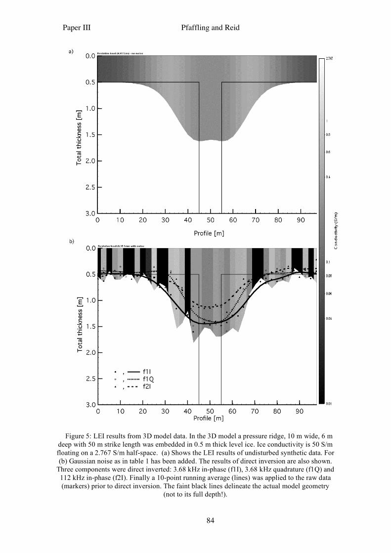
Paper III Pfaffling and Reid
84
Figure 5: LEI results from 3D model data. In the 3D model a pressure ridge, 10 m wide, 6 m
deep with 50 m strike length was embedded in 0.5 m thick level ice. Ice conductivity is 50 S/m floating on a 2.767 S/m half-space. (a) Shows the LEI results of undisturbed synthetic data. For (b) Gaussian noise as in table 1 has been added. The results of direct inversion are also shown.
Three components were direct inverted: 3.68 kHz in-phase (f1I), 3.68 kHz quadrature (f1Q) and 112 kHz in-phase (f2I). Finally a 10-point running average (lines) was applied to the raw data (markers) prior to direct inversion. The faint black lines delineate the actual model geometry
(not to its full depth!).
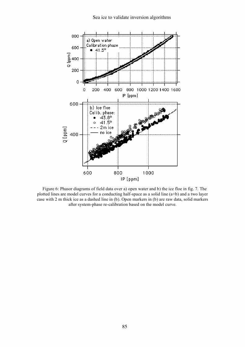
Sea ice to validate inversion algorithms
85
Figure 6: Phasor diagrams of field data over a) open water and b) the ice floe in fig. 7. The
plotted lines are model curves for a conducting half-space as a solid line (a+b) and a two layer case with 2 m thick ice as a dashed line in (b). Open markers in (b) are raw data, solid markers
after system-phase re-calibration based on the model curve.
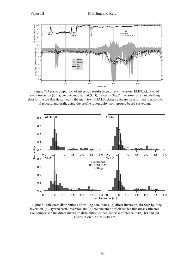
Paper III Pfaffling and Reid
86
Figure 7: Cross-comparison of inversion results from direct inversion (EMPEX), layered
earth inversion (LEI), conductance deficit (CD), “Step by Step” inversion (SbS) and drilling data for the ice floe described in the main text. HEM thickness data are transformed to absolute
freeboard and draft, using the profile topography from ground based surveying.
Figure 8: Thickness distributions of drilling data (bars), (a) direct inversion, (b) Step by Step
inversion, (c) layered earth inversion and (d) conductance deficit sea ice thickness estimates. For comparison the direct inversion distribution is included as a reference in (b), (c) and (d).
Distribution bin size is 10 cm.

87
PAPER IV

88
89
In-situ measurements of the direct-current conductivity of Antarctic sea ice: implications for airborne electromagnetic sounding of sea ice thickness (Abstract ID: 44A085) J. E. Reid1, A. Pfaffling2, A. P. Worby3 and J. R. Bishop4 1 School of Earth Sciences, University of Tasmania, Private Bag 79, Hobart, Tasmania 7001, Australia. Email: [email protected]. (Corresponding author). 2 Alfred Wegener Institute for Polar and Marine Research, Division of Climate Physics, P. O. Box 120161, 27515 Bremerhaven, Germany. Email: [email protected]
3 Antarctic Climate and Ecosystems Cooperative Research Centre and Australian Antarctic Division, Private Bag 80, Hobart, Tasmania 7001, Australia. Email: [email protected]
4 Mitre Geophysics Pty. Ltd., P. O. Box 974, Sandy Bay, Tasmania, 7006, Australia. Email: [email protected] Submitted Oct. 2005 to Annals of Glaciology Accepted for publication in Volume 44
Paper IV Reid, Pfaffling, Worby & Bishop
90
ABSTRACT Airborne, shipborne and surface low-frequency electromagnetic (EM) methods have
become widely applied to measure sea ice thickness. EM responses measured over sea ice depend mainly on the seawater conductivity and on the height of the sensor above the sea ice-seawater interface, but may be sensitive to the sea ice conductivity at high excitation frequencies. We have conducted in-situ measurements of direct-current (DC) conductivity of sea ice using standard geophysical geoelectrical methods. Sea ice thickness estimated from the geoelectrical sounding data was found to be consistently underestimated due to the pronounced vertical-to-horizontal conductivity anisotropy present in level sea ice. At five sites, it was possible to determine the approximate horizontal and vertical conductivities from the sounding data. The average horizontal conductivity was found to be 0.017 S/m, and that in the vertical direction to be 9-12 times higher. EM measurements over level sea ice are sensitive only to the horizontal conductivity. Numerical modelling has shown that the assumption of zero sea ice conductivity in interpretation of airborne EM data results in a negligible error in interpreted thickness for typical level Antarctic sea ice.
INTRODUCTION Low-frequency geophysical airborne electromagnetic (EM) methods have become an
important technique for remotely estimating sea ice thickness. Airborne EM methods have been used extensively in the Arctic (Kovacs et al. 1987; Kovacs and Holladay, 1990; Liu and Becker, 1990; Haas et al., 2002; Prinsenberg et al., 2002) and surveys have recently also been conducted in Antarctica (Pfaffling et al., 2004). Airborne EM methods provide reliable estimates of the thickness of level sea ice: the AWI HEM-Bird system considered in this study is able to determine modal thickness to within 10 cm for sea ice up to 3 m thick. Sea ice thickness may however be significantly over- or underestimated in areas of deformed sea ice (e.g. pressure ridges), as a result of both the relatively poor lateral resolution of low-frequency electromagnetic methods (e.g. Kovacs et al., 1995), and because data are routinely interpreted using simple, rapid ‘layered-earth’ interpretation algorithms.
Low-frequency electromagnetic techniques for measuring sea ice thickness rely on the fact that the electrical conductivity of sea ice is typically 1 – 2 orders of magnitude smaller than that of polar seawater. The EM transmitter therefore mainly induces eddy currents in the conductive seawater, and secondary magnetic fields measured at the EM receiver depend mainly on the altitude of the EM system above the sea ice-seawater interface, and on the seawater conductivity. Sea ice thickness (or snow plus sea ice thickness) is determined by subtracting the height of the EM system above the surface of the sea ice or snow, measured using a laser altimeter, from the depth to seawater estimated from the EM data. EM systems employed for sea ice thickness measurements utilise transmitter frequencies of a few hundred Hz to 200 kHz. In most interpretations of airborne EM sea ice thickness data, it is assumed that the conductivity of the sea ice is so low that it has no influence on the measured responses (e.g. Pfaffling et al., 2004). However, at higher transmitter frequencies (> 50 kHz), the measured airborne EM response may also be affected by the finite conductivity of the sea ice. The possibility exists that, in addition to thickness, sea ice conductivity can also be recovered from high frequency airborne electromagnetic data. Sea ice conductivity data could potentially be used to derive information on the bulk brine volume of sea ice, and hence to estimate its mechanical properties, as discussed by Kovacs (1996).
In situ DC sea ice conductivity
91
The ability of airborne EM methods to determine sea ice conductivity depends on the conductivity and thickness of the sea ice, and on the noise levels of the EM system. In this study, we have used in-situ direct-current (DC) geoelectrical methods to characterise the electrical conductivity of East Antarctic pack ice, in order to constrain interpretation of airborne EM sea ice thickness data acquired during September-October 2003 as part of the Antarctic Remote Ice Sensing Experiment (ARISE). Airborne EM data were acquired using the Alfred Wegener Institute (AWI) helicopter EM system (AWI HEM-Bird, Haas et al., 2002; Pfaffling et al., 2004). Theoretical modelling has been conducted in order to investigate the possibility of recovering sea ice conductivity from practical AWI HEM-Bird EM data.
DC electrical conductivity of sea ice Sea ice is an inhomogeneous composite of pure ice, brine, air and, at low
temperatures, precipitated salts. A number of authors have reported results of in-situ conductivity (or resistivity) measurements on Arctic and Antarctic sea ice. Thyssen et al., (1974), Kohnen (1976), Timco, (1979), and Buckley et al., (1986) report results of traditional direct-current resistivity measurements on sea ice. Morey et al., (1984) conducted time-domain reflectometry (TDR) measurements using ‘ladders’ of transmission lines frozen into growing Arctic sea ice, from which they were able to determine the DC conductivity. Becker et al., (1992) determined in-situ sea ice conductivity using high-frequency electromagnetic methods (8 MHz – 16 MHz) via measurements of the radiation resistance of a circular loop antenna placed on the surface of the ice.
Columnar sea ice exhibits a preferred fabric, with the orientation of the c-axes of the ice crystals predominantly horizontal, perpendicular to the direction of sea ice growth (Timco, 1979; Weeks and Ackley, 1986). Brine inclusions within the sea ice occur as thread-like cells arranged in thin, vertically-oriented layers. The shape of the brine cells is temperature-dependent: the cells are needle-shaped at low temperatures, but become disc-shaped at very warm temperatures (Timco, 1979). As the sea ice grows thicker, the entrapped brine drains out under gravity, forming vertically-aligned drainage tubes. Drainage tube diameters are typically between 0.1 cm and 1 cm, although diameters of up to 10 cm have been reported (Weeks and Ackley, 1986). Under certain temperature conditions, the drainage tubes may extend through the entire thickness of the sea ice (Golden, 2001).
The vertical orientation of both the brine cells and drainage tubes imparts a strong conductivity anisotropy to the sea ice, with the bulk conductivity in the vertical direction being higher than that in the horizontal direction (Thyssen et al., 1974). Thyssen et al. (1974) verified the presence of this conductivity anisotropy in-situ, by making direct measurements of the horizontal and vertical conductivities in the walls of a pit excavated in thick, undeformed Arctic sea ice. Buckley et al. (1986) detected a similar anisotropy in first-year Antarctic sea ice.
Paper IV Reid, Pfaffling, Worby & Bishop
92
RESULTS Direct-current measurements of sea ice conductivity were made using a Wenner
electrode array to conduct geoelectrical soundings (Figure 1a). Sixteen measurements were made on first-year pack ice within the region bounded by latitudes 63° 56.2’ S and 65° 14.3’ S and longitudes 109° 27.3’ E and 117° 44.5’ E. At each measurement site, the electrically-insulating snow cover was removed, and resistance measurements were made at a series of electrode separations ranging from a = 0.1 m to a = 10 m (Figure 1a) with the midpoint of the array fixed in position. For the purposes of data interpretation, the measured resistances were then transformed to apparent resistivity (ρa) according to the equation
aRa
!" 2= , (1)
where a is the electrode spacing (m) and R is the measured resistance (Ω).
The apparent resistivity vs. electrode separation data were then interpreted assuming a one-dimensional (layered) model, in which conductivity was assumed to be isotropic and to vary only with depth. The layered conductivity model was obtained using an iterative least-squares inversion process, in which the parameters of a starting model were automatically adjusted until the apparent resistivity curve computed for the model matched the field data. Figure 1(b) shows a typical comparison of observed data (symbols) with the calculated response of the best-fit three-layered model (dashed line) obtained via one-dimensional (1-D) inversion. Note that observed and calculated data have been plotted as apparent conductivity (σa = 1/ρa).
For the majority of the DC Wenner array measurements, the interpreted three-layered model comprised a thin, conductive near-surface layer, a thicker, less conductive middle layer, and a highly conductive lower layer (seawater). This conductivity distribution is typical of that for young (first-year) sea ice, and has been previously observed in both the Arctic (Thyssen et al., 1974) and Antarctic (Buckley et al., 1986). If the sea ice conductivity were isotropic, the sum of the interpreted thicknesses of the upper two layers would yield the depth to seawater below the surface, i.e. sea ice thickness. Figure 2 compares the sea ice thicknesses determined from the DC geoelectrical sounding data with the actual thickness obtained by drilling. The thickness interpreted from the DC sounding data consistently underestimates the drilled thickness. This is mainly the result of the high vertical conductivity of the sea ice, in comparison to that in the horizontal direction (Maillet, 1947; Thyssen et al., 1974). Another factor which may contribute to underestimation of the thickness is where the depth to seawater below the electrode array is highly variable: this renders the assumed 1-D interpretation model invalid and may result in erroneous interpreted sea ice thicknesses.
In addition to the DC soundings, thirteen azimuthal DC conductivity measurements were carried out at the field sites using an offset Wenner array (Watson and Barker, 1999), in order to identify any anisotropy of conductivity in the horizontal plane. The offset Wenner array is a variant of the traditional Wenner array which enables the effect of azimuthal variations in conductivity resulting from anisotropy to be distinguished from those which arise due to other effects, such as changes in sea ice thickness beneath the electrode array. Our offset Wenner data did not conclusively identify any anisotropy of conductivity in the horizontal plane. This result was expected, given that azimuthal conductivity variations develop as a result of a preferred horizontal orientation of the c-axes of the ice crystals, which can occur when sea ice forms in a fixed location relative to a prevailing current direction, such as for landfast ice (Weeks
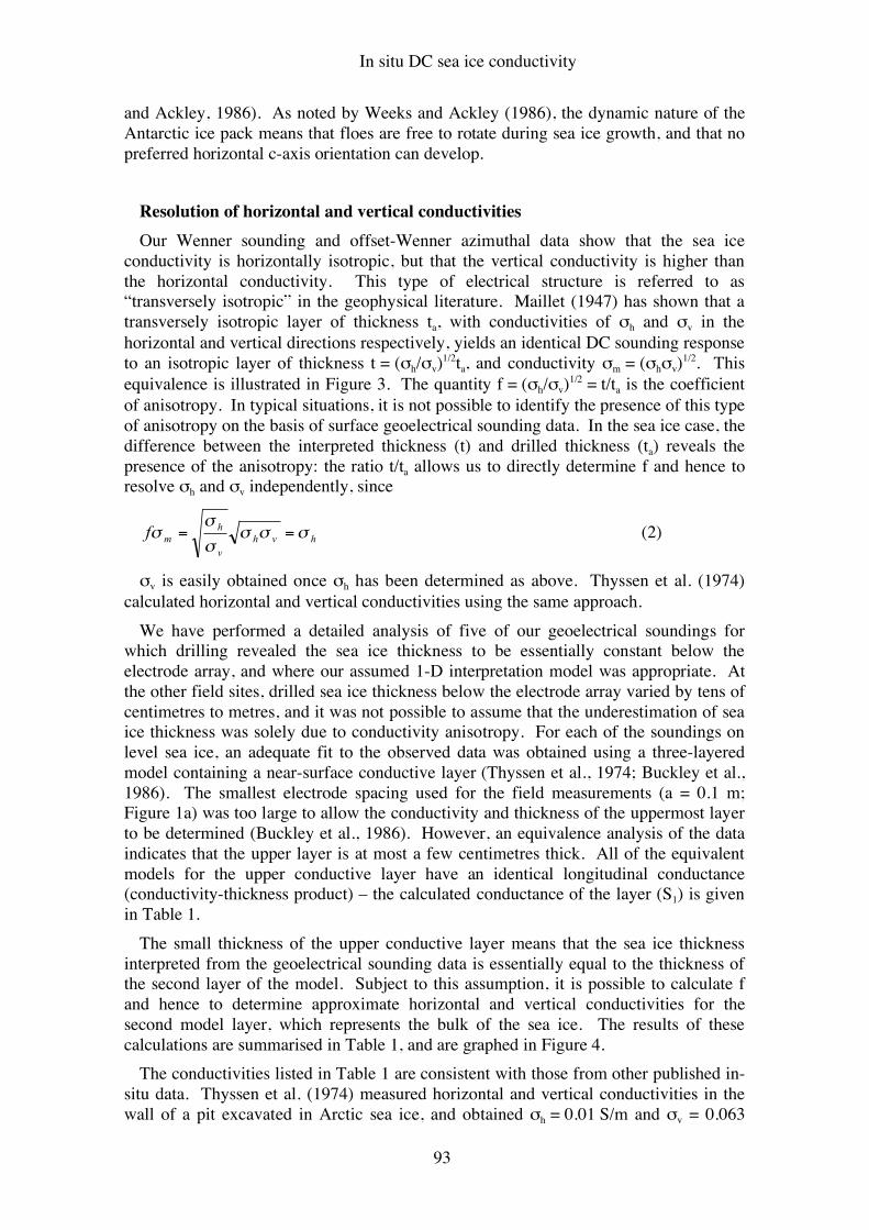
In situ DC sea ice conductivity
93
and Ackley, 1986). As noted by Weeks and Ackley (1986), the dynamic nature of the Antarctic ice pack means that floes are free to rotate during sea ice growth, and that no preferred horizontal c-axis orientation can develop.
Resolution of horizontal and vertical conductivities Our Wenner sounding and offset-Wenner azimuthal data show that the sea ice
conductivity is horizontally isotropic, but that the vertical conductivity is higher than the horizontal conductivity. This type of electrical structure is referred to as “transversely isotropic” in the geophysical literature. Maillet (1947) has shown that a transversely isotropic layer of thickness ta, with conductivities of σh and σv in the horizontal and vertical directions respectively, yields an identical DC sounding response to an isotropic layer of thickness t = (σh/σv)1/2ta, and conductivity σm = (σhσv)1/2. This equivalence is illustrated in Figure 3. The quantity f = (σh/σv)1/2 = t/ta is the coefficient of anisotropy. In typical situations, it is not possible to identify the presence of this type of anisotropy on the basis of surface geoelectrical sounding data. In the sea ice case, the difference between the interpreted thickness (t) and drilled thickness (ta) reveals the presence of the anisotropy: the ratio t/ta allows us to directly determine f and hence to resolve σh and σv independently, since
hvh
v
h
mf !!!!
!! == (2)
σv is easily obtained once σh has been determined as above. Thyssen et al. (1974) calculated horizontal and vertical conductivities using the same approach.
We have performed a detailed analysis of five of our geoelectrical soundings for which drilling revealed the sea ice thickness to be essentially constant below the electrode array, and where our assumed 1-D interpretation model was appropriate. At the other field sites, drilled sea ice thickness below the electrode array varied by tens of centimetres to metres, and it was not possible to assume that the underestimation of sea ice thickness was solely due to conductivity anisotropy. For each of the soundings on level sea ice, an adequate fit to the observed data was obtained using a three-layered model containing a near-surface conductive layer (Thyssen et al., 1974; Buckley et al., 1986). The smallest electrode spacing used for the field measurements (a = 0.1 m; Figure 1a) was too large to allow the conductivity and thickness of the uppermost layer to be determined (Buckley et al., 1986). However, an equivalence analysis of the data indicates that the upper layer is at most a few centimetres thick. All of the equivalent models for the upper conductive layer have an identical longitudinal conductance (conductivity-thickness product) – the calculated conductance of the layer (S1) is given in Table 1.
The small thickness of the upper conductive layer means that the sea ice thickness interpreted from the geoelectrical sounding data is essentially equal to the thickness of the second layer of the model. Subject to this assumption, it is possible to calculate f and hence to determine approximate horizontal and vertical conductivities for the second model layer, which represents the bulk of the sea ice. The results of these calculations are summarised in Table 1, and are graphed in Figure 4.
The conductivities listed in Table 1 are consistent with those from other published in-situ data. Thyssen et al. (1974) measured horizontal and vertical conductivities in the wall of a pit excavated in Arctic sea ice, and obtained σh = 0.01 S/m and σv = 0.063
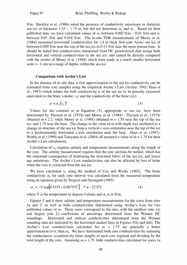
Paper IV Reid, Pfaffling, Worby & Bishop
94
S/m. Buckley et al. (1986) noted the presence of conductivity anisotropy in Antarctic sea ice of thickness 1.35 – 1.75 m, but did not determine σh and σv. Based on their published data, we have calculated values of σh between 0.002 S/m – 0.01 S/m and σv between 0.01 S/m and 0.034 S/m. The in-situ TDR measurements of Morey et al. (1984) measured horizontal conductivities for 1.4 m thick first-year Arctic sea ice of between 0.009 S/m near the top of the sea ice to 0.13 S/m near the more porous base. It should be noted that conductivities interpreted from DC geoelectrical data assign bulk horizontal and vertical conductivities to the sea ice, and cannot be directly compared with the results of Morey et al. (1984) which were made at a much smaller horizontal scale (~ 1 cm) at a range of depths within the sea ice.
Comparison with Archie’s Law
In the absence of in-situ data, a first approximation to the sea ice conductivity can be estimated from core samples using the empirical Archie’s Law (Archie, 1942; Haas et al., 1997) which relates the bulk conductivity σ of the sea ice to its porosity (assumed equivalent to the brine volume, vb) and the conductivity of the brine (σb):
( )mbbv!! = (3)
Values for the constant m in Equation (3), appropriate to sea ice, have been determined by Thyssen et al. (1974) and Morey et al. (1984). Thyssen et al., (1974) obtained m = 2.2, while Morey et al. (1984) obtained m = 1.55 near the top of the sea ice, and 1.75 near the base. The change in the value of m with depth was attributed to a change in structure of the sea ice from a vertical c-axis orientation near the top of the ice to a predominantly horizontal c-axis orientation near the base. Haas et al. (1997), Worby et al. (1999) and Tateyama et al. (2004) all assumed a value of m = 1.75 for their Archie’s Law calculations.
Calculation of vb requires salinity and temperature measurements along the length of the core. The salinity measurement requires that the core sections be melted, which has the important consequence of destroying the structural fabric of the sea ice, and hence any anisotropy. The Archie’s Law conductivities can also be affected by loss of brine when the core is extracted from the sea ice.
We have calculated vb using the method of Cox and Weeks (1983). The brine conductivity σb for each core interval was calculated from the measured temperature using an equation given by Stogryn and Desargant (1985)
[ ] CTTTb
o9.22,08755.05193.0exp !"+!=# (4)
where T is the temperature in degrees Celsius and σb is in S/m.
Figures 5 and 6 show salinity and temperature measurements for the cores from sites 1a and 2, as well as bulk conductivities determined using Archie’s Law for two published values of m. These cores correspond to the sites with the smallest (site 1a) and largest (site 2) coefficients of anisotropy determined from the Wenner DC soundings. Horizontal and vertical conductivities determined from the Wenner sounding data are indicated by the horizontal dashed lines in Figures 5(b) and 6(b). The Archie’s Law conductivities calculated for m = 1.75 are generally a better approximation to σv than σh. We have determined bulk core conductivities by summing the conductances (conductivity times length) of each core segment and dividing by the total length of the core. Assuming m = 1.75, bulk conductivities calculated for cores 1a
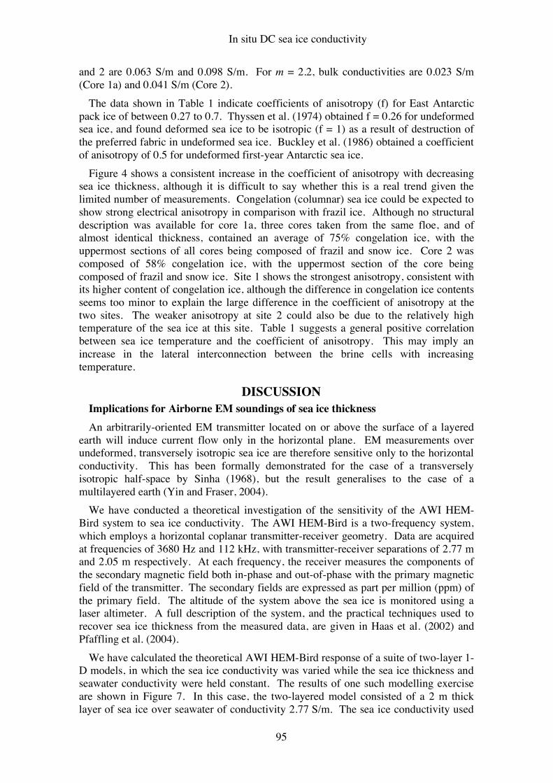
In situ DC sea ice conductivity
95
and 2 are 0.063 S/m and 0.098 S/m. For m = 2.2, bulk conductivities are 0.023 S/m (Core 1a) and 0.041 S/m (Core 2).
The data shown in Table 1 indicate coefficients of anisotropy (f) for East Antarctic pack ice of between 0.27 to 0.7. Thyssen et al. (1974) obtained f = 0.26 for undeformed sea ice, and found deformed sea ice to be isotropic (f = 1) as a result of destruction of the preferred fabric in undeformed sea ice. Buckley et al. (1986) obtained a coefficient of anisotropy of 0.5 for undeformed first-year Antarctic sea ice.
Figure 4 shows a consistent increase in the coefficient of anisotropy with decreasing sea ice thickness, although it is difficult to say whether this is a real trend given the limited number of measurements. Congelation (columnar) sea ice could be expected to show strong electrical anisotropy in comparison with frazil ice. Although no structural description was available for core 1a, three cores taken from the same floe, and of almost identical thickness, contained an average of 75% congelation ice, with the uppermost sections of all cores being composed of frazil and snow ice. Core 2 was composed of 58% congelation ice, with the uppermost section of the core being composed of frazil and snow ice. Site 1 shows the strongest anisotropy, consistent with its higher content of congelation ice, although the difference in congelation ice contents seems too minor to explain the large difference in the coefficient of anisotropy at the two sites. The weaker anisotropy at site 2 could also be due to the relatively high temperature of the sea ice at this site. Table 1 suggests a general positive correlation between sea ice temperature and the coefficient of anisotropy. This may imply an increase in the lateral interconnection between the brine cells with increasing temperature.
DISCUSSION Implications for Airborne EM soundings of sea ice thickness An arbitrarily-oriented EM transmitter located on or above the surface of a layered
earth will induce current flow only in the horizontal plane. EM measurements over undeformed, transversely isotropic sea ice are therefore sensitive only to the horizontal conductivity. This has been formally demonstrated for the case of a transversely isotropic half-space by Sinha (1968), but the result generalises to the case of a multilayered earth (Yin and Fraser, 2004).
We have conducted a theoretical investigation of the sensitivity of the AWI HEM-Bird system to sea ice conductivity. The AWI HEM-Bird is a two-frequency system, which employs a horizontal coplanar transmitter-receiver geometry. Data are acquired at frequencies of 3680 Hz and 112 kHz, with transmitter-receiver separations of 2.77 m and 2.05 m respectively. At each frequency, the receiver measures the components of the secondary magnetic field both in-phase and out-of-phase with the primary magnetic field of the transmitter. The secondary fields are expressed as part per million (ppm) of the primary field. The altitude of the system above the sea ice is monitored using a laser altimeter. A full description of the system, and the practical techniques used to recover sea ice thickness from the measured data, are given in Haas et al. (2002) and Pfaffling et al. (2004).
We have calculated the theoretical AWI HEM-Bird response of a suite of two-layer 1-D models, in which the sea ice conductivity was varied while the sea ice thickness and seawater conductivity were held constant. The results of one such modelling exercise are shown in Figure 7. In this case, the two-layered model consisted of a 2 m thick layer of sea ice over seawater of conductivity 2.77 S/m. The sea ice conductivity used
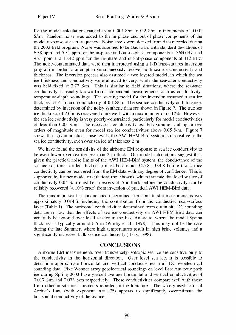
Paper IV Reid, Pfaffling, Worby & Bishop
96
for the model calculations ranged from 0.001 S/m to 0.2 S/m in increments of 0.001 S/m. Random noise was added to the in-phase and out-of-phase components of the model response at each frequency. Noise levels were derived from data recorded during the 2003 field program. Noise was assumed to be Gaussian, with standard deviations of 6.38 ppm and 5.81 ppm for the in-phase and out-of-phase components at 3680 Hz, and 9.24 ppm and 13.42 ppm for the in-phase and out-of-phase components at 112 kHz. The noise-contaminated data were then interpreted using a 1-D least-squares inversion program in order to attempt to simultaneously recover both sea ice conductivity and thickness. The inversion process also assumed a two-layered model, in which the sea ice thickness and conductivity were allowed to vary, while the seawater conductivity was held fixed at 2.77 S/m. This is similar to field situations, where the seawater conductivity is usually known from independent measurements such as conductivity-temperature-depth soundings. The starting model for the inversion assumed a sea ice thickness of 4 m, and conductivity of 0.1 S/m. The sea ice conductivity and thickness determined by inversion of the noisy synthetic data are shown in Figure 7. The true sea ice thickness of 2.0 m is recovered quite well, with a maximum error of 12%. However, the sea ice conductivity is very poorly-constrained, particularly for model conductivities of less than 0.05 S/m. The recovered conductivity exhibits variations of up to two orders of magnitude even for model sea ice conductivities above 0.05 S/m. Figure 7 shows that, given practical noise levels, the AWI HEM-Bird system is insensitive to the sea ice conductivity, even over sea ice of thickness 2 m.
We have found the sensitivity of the airborne EM response to sea ice conductivity to be even lower over sea ice less than 2 m thick. Our model calculations suggest that, given the practical noise limits of the AWI HEM-Bird system, the conductance of the sea ice (σh times drilled thickness) must be around 0.25 S - 0.4 S before the sea ice conductivity can be recovered from the EM data with any degree of confidence. This is supported by further model calculations (not shown), which indicate that level sea ice of conductivity 0.05 S/m must be in excess of 5 m thick before the conductivity can be reliably recovered (< 10% error) from inversion of practical AWI HEM-Bird data.
The maximum sea ice conductance determined from our in-situ measurements was approximately 0.014 S, including the contribution from the conductive near-surface layer (Table 1). The horizontal conductivities determined from our in-situ DC sounding data are so low that the effects of sea ice conductivity on AWI HEM-Bird data can generally be ignored over level sea ice in the East Antarctic, where the modal Spring thickness is typically around 0.5 m (Worby et al., 1998). This may not be the case during the late Summer, where high temperatures result in high brine volumes and a significantly increased bulk sea ice conductivity (Haas, 1998).
CONCLUSIONS Airborne EM measurements over transversely-isotropic sea ice are sensitive only to
the conductivity in the horizontal direction. Over level sea ice, it is possible to determine approximate horizontal and vertical conductivities from DC geoelectrical sounding data. Five Wenner-array geoelectrical soundings on level East Antarctic pack ice during Spring 2003 have yielded average horizontal and vertical conductivities of 0.017 S/m and 0.073 S/m respectively. These conductivities compare well with those from other in-situ measurements reported in the literature. The widely-used form of Archie’s Law (with exponent m = 1.75) appears to significantly overestimate the horizontal conductivity of the sea ice.
In situ DC sea ice conductivity
97
High frequency airborne EM data from the AWI HEM-Bird system have been shown to be insensitive to the electrical conductivity of undeformed East Antarctic sea ice, given the practical noise levels measured during the September 2003 field surveys. A much earlier field-based study of airborne EM measurements of sea ice thickness (Kovacs and Holladay, 1990) reached a similar conclusion for Arctic sea ice. The insensitivity of the system to sea ice conductivity was attributed to temperature related drift affecting both the system electronics and transmitter frequency. Although the AWI HEM-Bird contains internal calibration coils which allow in-flight calibration factor adjustments during high-altitude drift correction of the data, further reductions in the noise levels (possibly coupled with an increased maximum transmitter frequency) are required before sea ice conductivity measurements will be possible over the relatively thin sea ice typical of the East Antarctic.
ACKNOWLEGEMENTS This research was supported by Australian Antarctic Science Advisory Committee
grant 2381. We thank the officers and crew of RSV Aurora Australis for field support. Dr. Kazu Tateyama kindly provided the sea ice core temperature data used to produce Figures 5 and 6. We thank Angus Munro for assistance with data acquisition and processing.
Paper IV Reid, Pfaffling, Worby & Bishop
98
REFERENCES Archie, G. E. 1942. The electrical resistivity log as an aid in determining some reservoir
characteristics. Trans. Am. Inst. Min. Metall. Petr. Eng., 146, 54-62. Becker, A., D. C. Echert and G. B. White. 1992. Measurement of sea ice conductivity
by electromagnetic induction. Proc. Oceans 92, 748-752. Buckley, R. G., M. P. Staines and W. H. Robinson. 1986. In situ measurements of the
resistivity of Antarctic sea ice. Cold Regions Sci. Tech., 12, 285-290. Cox, G. F. N. and W. F. Weeks. 1983. Equations for determining the gas and brine
volumes in sea ice samples. J. Glaciol., 29, 306-316. Golden, K. M. 2001. Brine percolation and transport properties of sea ice. Annals of
Glaciology, 33, 28-36. Haas, C., S. Gerland, H. Eicken and H. Miller. 1997. Comparison of sea-ice thickness
measurements under summer and winter conditions in the Arctic using a small electromagnetic induction device. Geophysics, 62, 749-757.
Haas, C. 1998. Evaluation of ship-based electromagnetic-inductive thickness measurements of summer sea ice in the Bellingshausen and Amundsen Seas, Antarctica. Cold Regions Sci. Tech., 27, 1-16.
Haas, C., H. Edeler, M. Schurmann, J. Lobach and K.-P Sengpiel. 2002. First operation of AWI HEM-bird for sea ice thickness sounding. Proc. Jahrestagung der Deutschen Geophysikalischen Gesellschaft, 62, 36-38.
Kohnen, H. 1976. On the DC-resistivity of sea ice. Zeitschrift für Gletscherkunde and Glazialgeologie, XI(2), 143-154.
Kovacs, A., N. C. Valleau and J. S. Holladay. 1987. Airborne electromagnetic sounding of sea ice thickness and sub-ice bathymetry. Cold Regions Sci. Tech., 14, 289-311.
Kovacs, A. and J. S. Holladay. 1990. Sea ice thickness measurement using a small airborne electromagnetic sounding system. Geophysics, 55, 1327-1337.
Kovacs, A., J. S. Holladay and C. J. J. Bergeron. 1995. The footprint/altitude ratio for helicopter electromagnetic sounding of sea ice thickness: comparison of theoretical and field estimates: Geophysics, 60, 374–380.
Kovacs, A. 1996. Estimating the full-scale tensile, flexural and compressive strength of first-year ice. Cold Regions Research and Engineering Laboratory Report 96-11.
Liu, G. and A. Becker. 1990. Two-dimensional mapping of sea ice keels with airborne electromagnetics. Geophysics, 55, 239-248.
Maillet, R. 1947. The fundamental equations of electrical prospecting. Geophysics, 12, 529-555.
Morey, R. M., A. Kovacs and G. F. N. Cox. 1984. Electromagnetic properties of sea ice: Cold Regions Sci. Tech. 9, 53-75.
Pfaffling, A., C. Haas, and J. E. Reid. 2004. Empirical processing of HEM data for sea ice thickness mapping. Expanded abstracts, 10th European Meeting of Environmental and Engineering Geophysics, Utrecht, The Netherlands.
Prinsenberg, S. J., S. Holladay and J. Lee. 2002. Measuring ice thickness with EISFlow, a fixed-mounted helicopter electromagnetic-laser system. Proc. 12th Intl. conference on offshore and polar engineering, Kitakyushu, Japan, Volume 1, Intl. Soc. Offshore and Polar Eng., 737-740.
Sinha, A. K. 1968. Electromagnetic fields of an oscillating magnetic dipole over an anisotropic earth. Geophysics, 33, 346-353.
Stogryn, A. and G. J. Desargant. 1985. The dielectric properties of brine in sea ice at microwave frequencies. IEEE Trans. Antennas and propagation, AP-33, 523-532.
In situ DC sea ice conductivity
99
Tateyama, K., S. Uto, K. Shirasawa and H. Enomoto, H. 2004. Electromagnetic-inductive measurements for the undeformed and deformed sea-ice and snow in the East Antarctic. Proc. 14th Intl. conference on offshore and polar engineering, Toulon, France. Volume 1, Intl. Soc. Offshore and Polar Eng., 806-812.
Timco, G. W. 1979. An analysis of the in-situ resistivity of sea ice in terms of its microstructure. J. Glaciol., 22, 461-471.
Thyssen, F., H. Kohnen, M. V. Cowan, and G. W. Timco. 1974. DC resistivity measurements on the sea ice near Pond Inlet, N. W. T. (Baffin Island). Polarforschung, 44, 117-126.
Watson, K. A. and R. D. Barker. 1999. Differentiating anisotropy and lateral effects using azimuthal resistivity offset Wenner soundings. Geophysics, 64, 739-745.
Weeks, W. F. and S. F. Ackley. 1986. The growth, structure and properties of sea ice. In Untersteiner, N., ed. The geophysics of sea ice, Plenum Press, 9-164.
Worby, A. P., R. A. Massom, I. Allison, V. I. Lytle and P. Heil. 1998. East Antarctic sea ice: a review of its structure, properties and drift. In Jeffries, M. O. ed. Antarctic sea ice: physical processes, interactions and variability, Antarctic Research Series, 74, 41-67.
Worby, A. P., P. W. Griffin, V. I. Lytle and R. A. Massom. 1999. On the use of electromagnetic induction sounding to determine winter and spring sea ice thickness in the Antarctic. Cold Regions Sci. Tech., 29, 49-58.
Yin, C. and D. C. Fraser. 2004. The effect of the electrical anisotropy on the response of helicopter-borne frequency-domain electromagnetic systems. Geophys. Prosp., 52, 399-416.
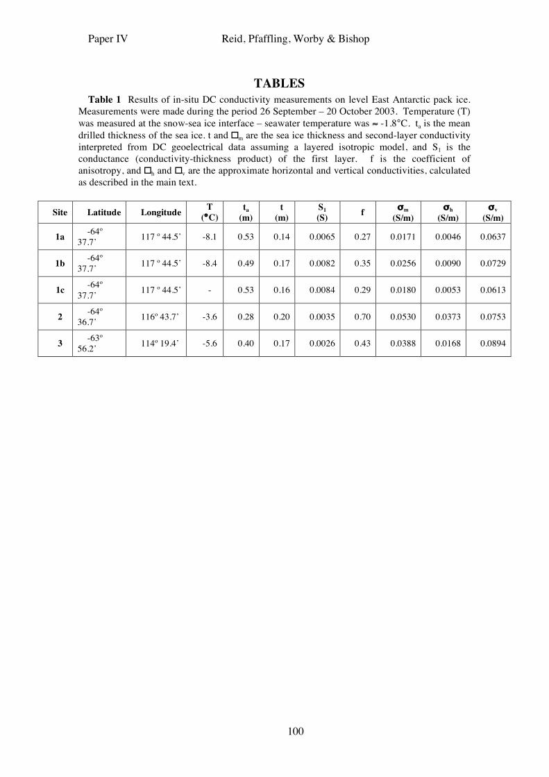
Paper IV Reid, Pfaffling, Worby & Bishop
100
TABLES Table 1 Results of in-situ DC conductivity measurements on level East Antarctic pack ice.
Measurements were made during the period 26 September – 20 October 2003. Temperature (T) was measured at the snow-sea ice interface – seawater temperature was ≈ -1.8°C. ta is the mean drilled thickness of the sea ice. t and � m are the sea ice thickness and second-layer conductivity interpreted from DC geoelectrical data assuming a layered isotropic model, and S1 is the conductance (conductivity-thickness product) of the first layer. f is the coefficient of anisotropy, and � h and � v are the approximate horizontal and vertical conductivities, calculated as described in the main text.
Site Latitude Longitude T
(°C) ta
(m) t
(m) S1 (S) f σm
(S/m) σh
(S/m) σv
(S/m)
1a -64º 37.7’ 117 º 44.5’ -8.1 0.53 0.14 0.0065 0.27 0.0171 0.0046 0.0637
1b -64º 37.7’ 117 º 44.5’ -8.4 0.49 0.17 0.0082 0.35 0.0256 0.0090 0.0729
1c -64º 37.7’ 117 º 44.5’ - 0.53 0.16 0.0084 0.29 0.0180 0.0053 0.0613
2 -64º 36.7’ 116º 43.7’ -3.6 0.28 0.20 0.0035 0.70 0.0530 0.0373 0.0753
3 -63º 56.2’ 114º 19.4’ -5.6 0.40 0.17 0.0026 0.43 0.0388 0.0168 0.0894
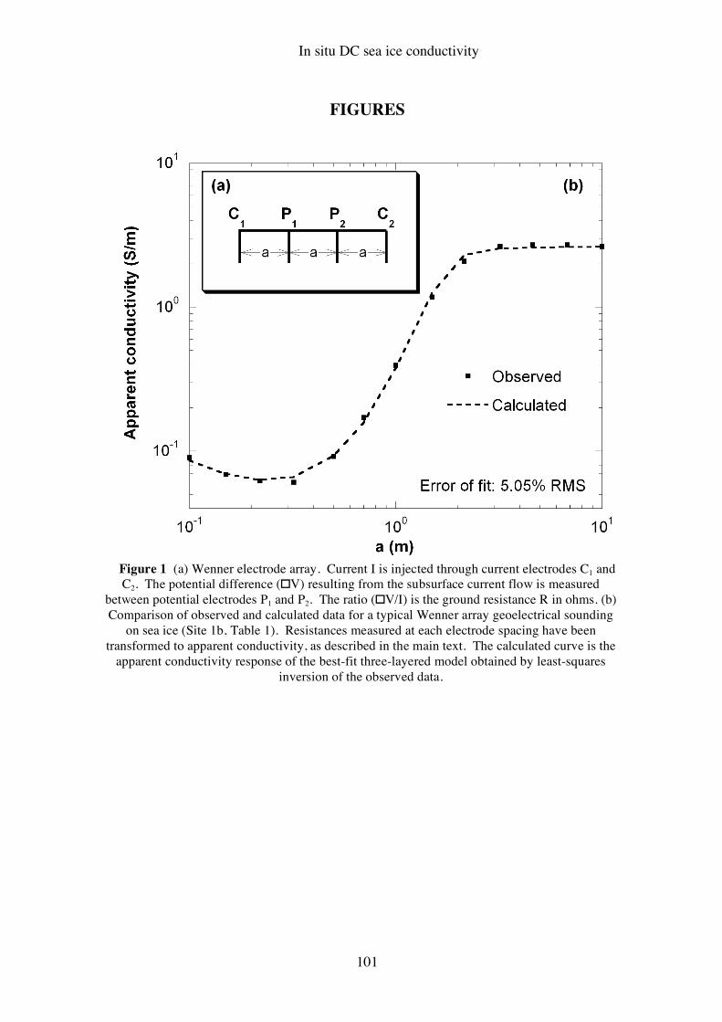
In situ DC sea ice conductivity
101
FIGURES
Figure 1 (a) Wenner electrode array. Current I is injected through current electrodes C1 and C2. The potential difference (� V) resulting from the subsurface current flow is measured
between potential electrodes P1 and P2. The ratio (� V/I) is the ground resistance R in ohms. (b) Comparison of observed and calculated data for a typical Wenner array geoelectrical sounding
on sea ice (Site 1b, Table 1). Resistances measured at each electrode spacing have been transformed to apparent conductivity, as described in the main text. The calculated curve is the
apparent conductivity response of the best-fit three-layered model obtained by least-squares inversion of the observed data.
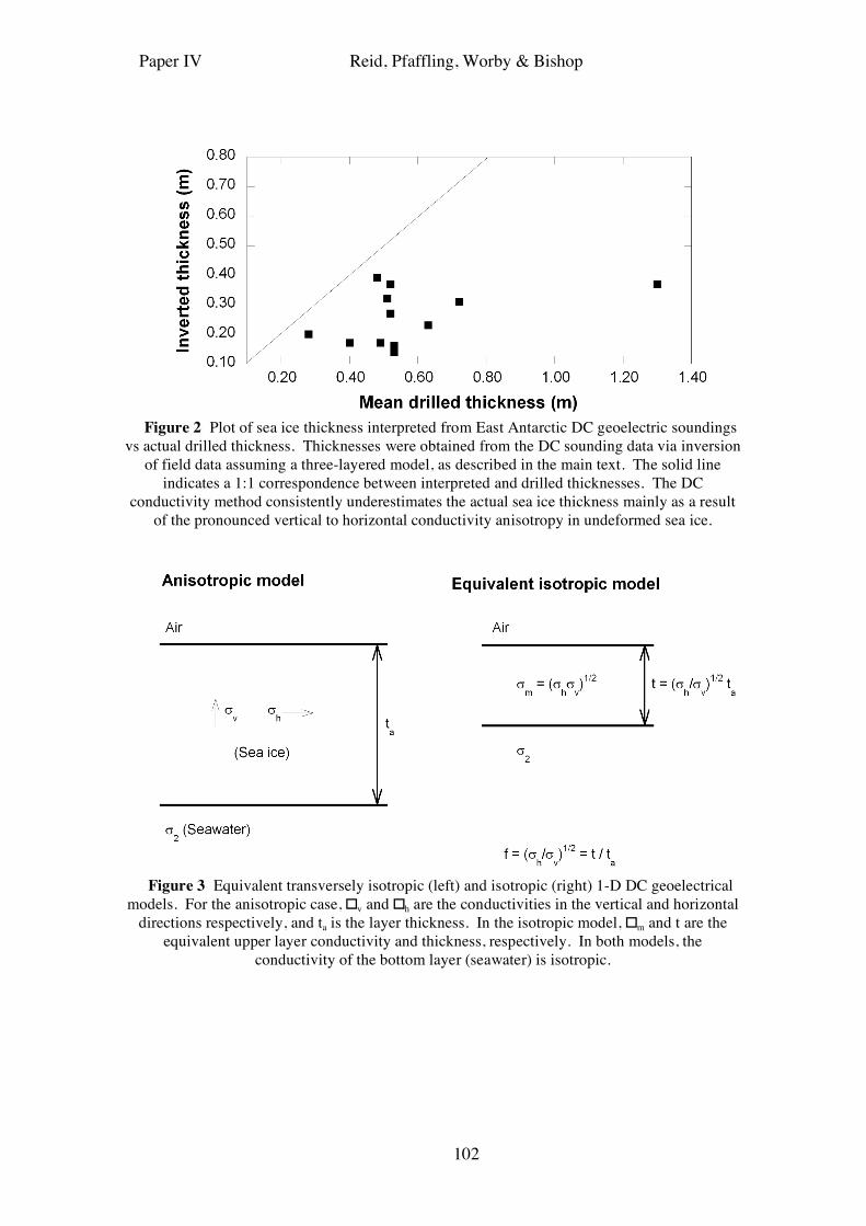
Paper IV Reid, Pfaffling, Worby & Bishop
102
Figure 2 Plot of sea ice thickness interpreted from East Antarctic DC geoelectric soundings
vs actual drilled thickness. Thicknesses were obtained from the DC sounding data via inversion of field data assuming a three-layered model, as described in the main text. The solid line
indicates a 1:1 correspondence between interpreted and drilled thicknesses. The DC conductivity method consistently underestimates the actual sea ice thickness mainly as a result
of the pronounced vertical to horizontal conductivity anisotropy in undeformed sea ice.
Figure 3 Equivalent transversely isotropic (left) and isotropic (right) 1-D DC geoelectrical
models. For the anisotropic case, � v and � h are the conductivities in the vertical and horizontal directions respectively, and ta is the layer thickness. In the isotropic model, � m and t are the
equivalent upper layer conductivity and thickness, respectively. In both models, the conductivity of the bottom layer (seawater) is isotropic.
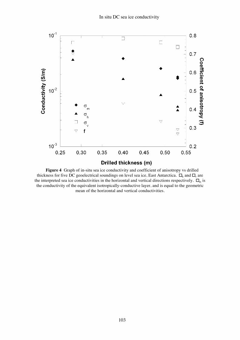
In situ DC sea ice conductivity
103
Figure 4 Graph of in-situ sea ice conductivity and coefficient of anisotropy vs drilled
thickness for five DC geoelectrical soundings on level sea ice, East Antarctica. � h and � v are the interpreted sea ice conductivities in the horizontal and vertical directions respectively. � m is the conductivity of the equivalent isotropically-conductive layer, and is equal to the geometric
mean of the horizontal and vertical conductivities.
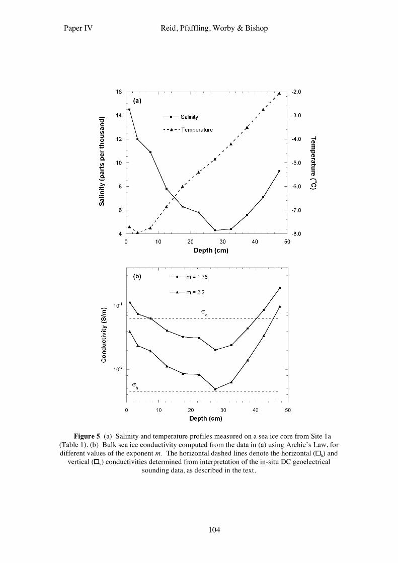
Paper IV Reid, Pfaffling, Worby & Bishop
104
Figure 5 (a) Salinity and temperature profiles measured on a sea ice core from Site 1a
(Table 1). (b) Bulk sea ice conductivity computed from the data in (a) using Archie’s Law, for different values of the exponent m. The horizontal dashed lines denote the horizontal (� h) and
vertical (� v) conductivities determined from interpretation of the in-situ DC geoelectrical sounding data, as described in the text.
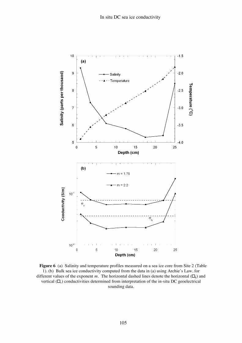
In situ DC sea ice conductivity
105
Figure 6 (a) Salinity and temperature profiles measured on a sea ice core from Site 2 (Table
1). (b) Bulk sea ice conductivity computed from the data in (a) using Archie’s Law, for different values of the exponent m. The horizontal dashed lines denote the horizontal (� h) and
vertical (� v) conductivities determined from interpretation of the in-situ DC geoelectrical sounding data.
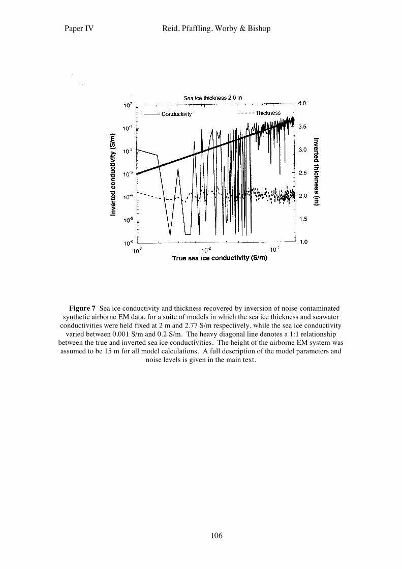
Paper IV Reid, Pfaffling, Worby & Bishop
106
Figure 7 Sea ice conductivity and thickness recovered by inversion of noise-contaminated
synthetic airborne EM data, for a suite of models in which the sea ice thickness and seawater conductivities were held fixed at 2 m and 2.77 S/m respectively, while the sea ice conductivity
varied between 0.001 S/m and 0.2 S/m. The heavy diagonal line denotes a 1:1 relationship between the true and inverted sea ice conductivities. The height of the airborne EM system was assumed to be 15 m for all model calculations. A full description of the model parameters and
noise levels is given in the main text.