health, aging and childhood socio-economic conditions in mexico
TRANSCRIPT
H
Fa
b
a
ARRAA
JIJOO
KHAM
1
dbgaal12l
d
aEfwmC
Sf
0d
Journal of Health Economics 29 (2010) 630–640
Contents lists available at ScienceDirect
Journal of Health Economics
journa l homepage: www.e lsev ier .com/ locate /econbase
ealth, aging and childhood socio-economic conditions in Mexico�
ranque Grimarda, Sonia Laszloa,∗, Wilfredo Limb
McGill University, CanadaColumbia University, USA
r t i c l e i n f o
rticle history:eceived 25 February 2009eceived in revised form 22 June 2010ccepted 1 July 2010vailable online 7 July 2010
EL classification:12
a b s t r a c t
We investigate the long-term effect of childhood socio-economic conditions on the health of the elderlyin Mexico. We utilize a panel of individuals aged 50 and above from the Mexican Health and Aging Surveyand find that the conditions under which the individual lived at the age of 10 affect health in old age, evenaccounting for education and income. This paper contributes to the literature of the long-term effects ofchildhood socio-economic status by being the first, to our knowledge, to consider exclusively the case ofthe elderly in a developing country.
© 2010 Elsevier B.V. All rights reserved.
141215
eywords:ealth
dmntceocut
gingexico
. Introduction
Recent research from both developed and developing countriesocuments the importance of childhood socio-economic status onoth health and economic outcomes later in life. From their ori-ins in the income gradient literature (Case et al., 2002; Curriend Stabile, 2003), studies of the effects of socio-economic statusmong the elderly (Case et al., 2005; Buckley et al., 2004) and thoseinking birth outcomes to health in adulthood (Currie and Hyson,999; Almond, 2006; Currie and Moretti, 2007; Oreopoulos et al.,
008; Maccini and Yang, 2009) suggest that conditions in childhoodead to long-lasting health effects, at least in developed countries.With increased living standards and higher life expectancy,
eveloping countries face a dual challenge of managing an epi-
� We thank seminar participants at McGill University (department of Economicsnd Social Statistics seminars), participants from the 2007 NEUDC and Canadianconomic Association meetings and the Third Annual Hewlett/PRB Research Con-erence at UC Dublin, 2009. Our paper has also greatly benefited from discussionsith Gustavo Bobonis, Shelley Clark and Amélie Quesnel-Vallée, and from com-ents made by two anonymous referees. We also thank the Population Studies
enter at the University of Pennsylvania for allowing us to use their data.∗ Corresponding author at: Department of Economics, McGill University, 855
herbrooke Street West, Montreal, Quebec, H3A 2T7, Canada. Tel.: +1 514 398 1924;ax: +1 514 398 4938.
E-mail address: [email protected] (S. Laszlo).
a
hcaep(cwpc
cac
167-6296/$ – see front matter © 2010 Elsevier B.V. All rights reserved.oi:10.1016/j.jhealeco.2010.07.001
emiological and a demographic transition. This combinationeans that chronic degenerative diseases become more promi-
ent among these countries’ aging populations. The elderly arehus experiencing increasing rates of chronic, in addition toommunicable, disease. Yet, despite the growing proportion oflderly persons in developing countries, the majority of analysesf the effects of socio-economic status on health in these countriesontinues to focus on children or on the economically active pop-lations, and those that do consider the elderly do not investigatehe long-term effects of childhood conditions (Mete, 2005; Roynd Chaudhuri, 2008).
We contribute to the literature on the long-run effects of child-ood conditions on health by providing evidence from a developingountry. While recent work in development economics by Maccinind Yang (2009) and Akresh et al. (forthcoming) focus on theseffects for adults in general, we focus our lens on the elderly. We useanel data from the 2001/2003 Mexican Health and Aging SurveyMHAS) to assess the long-run impact of childhood socio-economiconditions on health among individuals aged 50 and above. Facedith this dual demographic and epidemiological transition, Mexicorovides a unique setting in which to study the role of childhood
onditions on elderly health outcomes.We begin in Section 2 by highlighting the conceptual frameworkommonly adapted in the literature (Grossman, 1972; Maccinind Yang, 2009). We then turn to the MHAS and discuss theonstruction of the main variables of interest in Section 3. We con-
alth E
ssKm
reloeTsathi
odrse
ssrcpcpfvtd
2
ehmBaTpd
ueotoechispi
oT
(ufhmie
malcpt
hcic1sthA
eaoicihgf
H
Br�a
H
waChclng
H
Bt
F. Grimard et al. / Journal of He
truct a measure of good health from self-reported status. Becauseuch subjective measures are measured with error (Crossley andennedy, 2002; Baker et al., 2004), we provide evidence that thiseasure is nonetheless correlated with self-reported ailments.In Section 4, we present the results of a reduced form
elationship between health status in old age and childhood socio-conomic conditions. We find that conditions at age 10 indicatingow socio-economic status have long-lasting and negative impactsn an individual’s health. We find that this effect persists, yet weak-ns, when we control for an individual’s education and wealth.hat the effect weakens points to the likelihood that childhoodocio-economic conditions influence health via their role in theccumulation of human capital and thus future earnings poten-ial. That the effect persists suggests that childhood circumstancesave an effect beyond adult socio-economic conditions by directly
nfluencing health in adulthood.We check for the robustness of our results to several limitations
f our empirical strategy. Because our dependent and indepen-ent variables may possibly be measured with error, we check forobustness of our results using alternative measures of health andocio-economic conditions. Our results are robust to these consid-rations.
Because our variables of childhood circumstances do not mea-ure conditions in utero or early infancy (which the literatureuggests is most important) we consider the possibility that ouresults are driven by endogeneity between health in old age andonditions before age 10. The data do not provide us with anylausible exogenous variation or strong instrument for childhoodircumstances. However, we make an attempt by appealing toarental background variables (such as parental education and theather’s occupation) to eliminate one possible source of omittedariable bias. We still find persistent effects of childhood condi-ions, especially among women. In Section 5, we conclude andiscuss the policy implications of our results.
. Conceptual background
We seek to establish the long-run impact of childhood socio-conomic status (CSES) on health among the elderly. The literatureas proposed several mechanisms through which this relationshipay operate. First, life-course models (Kuh and Wadsworth, 1993;
en-Slomo and Kuh, 2002) emphasize the role that CSES can play ondult health through its effect on adult socio-economic status (SES).hese models imply that good adult socio-economic outcomes canartially compensate for poor early childhood socio-economic con-itions (Graham, 2002).
Life-course models operate in the following way. An individ-al’s health at any given time is a function of her SES (income,ducation, etc.) at that time and of her health stock in previous peri-ds. Similarly, socio-economic conditions at any point in time arehemselves a function of health in previous periods: poor health inne period might negatively affect an individual’s ability to acquireducation and may also have a detrimental effect on her earningsapabilities. The determination of health among the elderly thusas a recursive nature since health stock at any given point in time
s a function of health stock in the previous period. This recursivetructure, both in terms of health stock and SES, implies that initialeriod health stock and initial SES (be it in utero, at birth or in early
nfancy) will carry through to adulthood and old age.1
1 For good discussions of the socio-economic determinants of health in devel-ping economies, see Glewwe and Miguel (2008), Mwabu (2008), and Strauss andhomas (2008).
epi
ifaSp
conomics 29 (2010) 630–640 631
Note that this process can be reconciled with the Grossman1972) model of gross investment if we consider that an individ-al’s ability to invest in health from one period to the next is aunction of her SES. Wealthier individuals are better able to affordealth investments. Similarly, more educated individuals investore in health partly because their education makes them wealth-
er and partly through the non-pecuniary benefits of an increasedducation (e.g. knowledge).
Second, the critical-period programming (or foetal origins)odel (Barker, 1998; Barker et al., 2002) links conditions in utero,
t birth or in early infancy with lower health trajectories over theife-course. Specifically, there is growing biological evidence thatonditions during such a critical period can change an individual’shysiology causing a permanent and downward shift in her healthrajectory.
According to Barker (1998), nutritional deficiencies in uteroave been linked to chronic health problems in old age (such asoronary heart disease and stroke). Explanations based on biolog-cal research suggest that these effects are driven by “permanenthanges” in the “body’s structure, physiology and metabolism (p.3)”. Citing work by Reynaldo Martorell, Elo and Preston (1992)uggest that adult height is “essentially determined by events inhe first three years of life (p. 193).” Thus, any effects of CSES oneight can have long-lasting impacts on health (Case et al., 2005;lmond, 2006; Strauss and Thomas, 2008; Maccini and Yang, 2009).
Our conceptual framework follows from Grossman (1972) andspecially Maccini and Yang (2009). Specifically, we consider thatn individual’s health in old age (Ht) is a function of health statesver her life-time including initial health (H0, H1, . . ., Ht−1), healthnputs purchased and consumed over her life-time (N1, . . ., Nt),haracteristics of her location over her life-time (C0, . . ., Ct) whichncludes community infrastructure and disease environment, ander time-invariant demographic characteristics (X). These inputsenerate a health production function that can be summarized asollows:
t = H(H0, H1, . . . , Ht−1, N1, . . . , Nt, C0, . . . , Ct, X)
ecause this process is recursive in health stock, sequentiallyeplacing H� with its expression for each time period from � = 0 to= t − 1 leads to the following reduced form expression for healtht time t:
t = h(H0, N1, . . . , Nt, C0, . . . , Ct, X) (1)
hich is precisely the approach in Maccini and Yang (2009), anpproach we co-opt here. Specifically, we focus on the effect ofSES on health in old age and so we turn our attention to initialealth, H0, which relates to ‘critical-period programming’ whereonditions in utero or in infancy have measurable implications forong-run health. In the same vein, we take CSES to be a determi-ant of initial health. Initial health is also influenced by unobservedenetic factors (G) and initial community-level characteristics:
0 = g(CSES, G, C0) (2)
oth the life-course and critical-period programming models implyhat health in ‘old age’ is influenced by CSES conditions. The differ-nce between the two classes of models is that the critical-periodrogramming model allows for CSES to have an effect on health
ndependently of their effect via adult SES.The questions we explore are first whether CSES affects health
n old age and second whether this effect persists when controllingor adult SES. We expect that life-course mechanisms are present,nd so our empirical strategy will consider the influence of adultES. However, we seek to uncover evidence of the critical-periodrogramming hypothesis. The exercise we conduct summarizes as
6 alth E
fsifSottchapaauwpwt
3
3
ariranawvdCask
3
ssteow‘ts
batb
oaa
h
hKotattsie
tr(brohpr(zroom
−tfamirpsdrhootattabsba
mWosrr
32 F. Grimard et al. / Journal of He
ollows. If critical-period programming is not an issue, then CSEShould affect adult health only via its effect on adult SES. This wouldmply that we could consider CSES an instrumental variable (IV)or adult SES which are thought to be endogenous (Thomas andtrauss, 2008). However, if we find that the adult health effectsf CSES persist even when controlling for adult SES, then we havewo candidate explanations. The first explanation would be thathere is evidence that critical-period programming is an importanthannel and we would not reject the critical-period programmingypothesis that early life circumstances have permanent effects onn individual’s health. In other words, both life-course and critical-eriod programming mechanisms operate and CSES cannot be useds IV for adult SES. The second explanation is that we are not doinggood job at capturing CSES or adult SES. If instead CSES are pickingp a component of adult SES which are measured with error, then itould be misleading to conclude that both life-course and critical-eriod programming mechanisms operate. Our research strategyill be to conduct a series of robustness checks to try to rule out
his second explanation.
. Data
.1. Mexican health and aging study (MHAS)
The MHAS is a 2-year panel study modeled after the U.S. Healthnd Retirement Study.2 At its baseline in 2001, it was nationallyepresentative of Mexicans born prior to 1951 (i.e. age 50 and oldern 2000). The survey includes information on health measures (self-eports of conditions and functional status), background (educationnd childhood living conditions), family demographics, and eco-omic measures (wage and non-wage income and assets). In ournalysis we keep non-proxy interview observations for individualsho responded both in 2001 and in 2003. In addition, we keep indi-
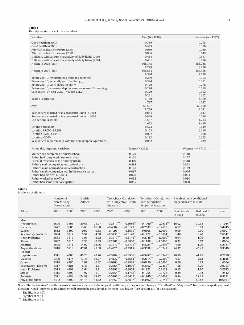
iduals with complete information on the key variables. Namely werop respondents with missing information on childhood health,SES, or education. These restrictions yield a sample of 3818 mennd 4392 women born before 1951. Descriptive statistics are pre-ented in Table 1, and below we describe the construction of theey dependent and independent variables.
.2. Dependent variables – health outcomes
To construct a measure of good health, we utilize MHAS data onelf-reported quality of health, based on the question “Would youay your health is excellent, very good, good, fair, or poor?” Fromhese responses, we define a binary indicator of “Good Health” thatquals 1 if the response is ‘excellent’, ‘very good’, or ‘good’, and 0therwise. While this definition is arbitrary, later in this section,e compare this to a more stringent definition of ‘good health’ as
excellent’ or ‘very good’. We find a stronger correlation betweenhe former definition (‘excellent’, ‘very good’, or ‘good’) and severalelf-reported chronic conditions, lending support for the former.
We observe in Table 1 that 38% of men and 30% of women reporteing in good health in 2003. This contrasts with higher rates of 44%nd 32% for men and women, respectively, in 2001. We attributehis difference to the fact that respondents have aged by two yearsetween rounds and consequently report somewhat worse health.
This measure of health status is often used in predicting healthutcomes such as health care utilization and mortality (Buckley etl., 2004; Roy and Chaudhuri, 2008) and is used widely in this liter-ture (Case et al., 2005; Maccini and Yang, 2009). Yet, self-reported
2 Data and information from MHAS can be obtained from their website,ttp://www.mhas.pop.upenn.edu/.
l
Htttas
conomics 29 (2010) 630–640
ealth measures are prone to measurement error (Crossley andennedy, 2002; Baker et al., 2004). Because of the subjectivity ofur measure, we utilize supplementary information contained inhe MHAS by comparing this measure of health to more objective,lbeit self-reported, indicators. While we cannot entirely eliminatehe problem of measurement error, we try to reduce the likelihoodhat our results are driven by the subjectivity of the health mea-ure. Though our health measure is imprecisely measured, since its the dependent variable, the error is absorbed in the regressionrror and is thus not of great concern.
The MHAS asked respondents whether they suffered from par-icular ailments (hypertension, diabetes, cancer, heart disease,espiratory illness, stroke and arthritis) in the last 2 years or eversee Table 2 for prevalence). Table 2 provides the correlationsetween our subjective measure of good health and having expe-ienced each of the individual ailments. In all cases, the directionf the correlation confirms the validity of the subjective measure:aving suffered from hypertension, diabetes, cancer, respiratoryroblems, heart problems, strokes or arthritis is negatively cor-elated with being in good health. These correlations are alwayssave for cancer in 2001) very strongly significantly different fromero. We also construct an aggregate ailment measure as those whoeport having ever or in the last two years suffered from any onef these seven ailments. We find that 45–47% of men and 61–64%f women report having experienced at least one of the seven ail-ents.However, the magnitudes of these correlations only range from
0.02 to −0.41 for each individual ailment, and the aggregate (inhe last row) has a correlation over −0.43. This could be due to theact that respondents in ill-health are suffering from ailments thatre not listed in the above. This could also be a result of measure-ent error: given the subjectivity of the good health measure, it
s possible that respondents who suffer from an ailment actuallyeport being in ‘good’ health. This is in fact the case, for exam-le, for 25% of respondents who report hypertension in 2001 and,urprisingly, 29% of respondents who report in 2001 having beeniagnosed with cancer. Thus, we check for the robustness of ouresults by considering ‘good’ health responses to the quality ofealth variable as being in ‘bad’ health as an alternative measure:ur constructed measure may be biased because of the presencef false negatives (the ill who report ‘good’ health). The correla-ions of this alternative constructed measure of good health arelso reported in Table 2. We immediately observe that the magni-udes and significance of the correlations fall drastically (except inhe case of cancer in 2003, where cell size is very small). While thislternative measure might pick up those individuals who reportedeing in ‘good’ health despite suffering from an ailment, it wouldeem that the possibility of a false positive (the healthy who reporteing in ‘good’ health but considered to be in ‘bad’ health in thelternative measure) is more problematic.
The subjectivity of health status suggests that these measuresay be picking up perceptions of health rather than health itself.e address this concern in three ways. First, the last three columns
f Table 2 consider only those individuals who report good healthtatus in 2001, and we compare their ailment outcomes across theireported health status in 2003. We see that conditioning on self-eporting good health in 2001 those reporting bad health two yearsater have significantly worse ailment outcomes.
Second, we exploit the MHAS’s module on “Functionality andelp” and consider respondents’ reported difficulties with Activi-
ies of Daily Living (ADLs). We constructed a binary variable takinghe value 1 if respondents reported difficulty with any of 10 activi-ies (walking, sitting, getting up, climbing stairs, stooping, reachingrm over shoulder, pulling, lifting, picking and dressing). Table 1hows that between 43% and 45% of men report difficulties with
F. Grimard et al. / Journal of Health Economics 29 (2010) 630–640 633
Table 1Descriptive statistics of main variables.
Variable Men (N = 3818) Women (N = 4392)
Good health in 2003 0.380 0.295Good health in 2001 0.443 0.320Alternative health measure (2003) 0.059 0.039Alternative health measure (2001) 0.086 0.049Difficulty with at least one activity of daily living (2003) 0.434 0.587Difficulty with at least one activity of daily living (2001) 0.451 0.620Height in 2003 (cm) 166.348 155.718
8.729 8.280Height in 2001 (cm) 166.634 156.126
8.540 7.788Before age 10, residence had toilet inside house 0.269 0.302Before age 10, generally go to bed hungry 0.344 0.291Before age 10, wore shoes regularly 0.779 0.778Before age 10, someone slept in same room used for cooking 0.220 0.198CSES index (0 = best CSES, 1 = worst CSES) 0.379 0.352
0.291 0.292Years of education 5.180 4.370
4.787 4.022Age 61.537 60.588
8.780 8.311Respondent married or in consensual union in 2001 0.854 0.617Respondent married or in consensual union in 2003 0.839 0.586Log per capita assets 11.587 11.724
1.462 1.460Location 100,000+ 0.574 0.619Location 15,000–99,999 0.153 0.146Location 2500–14,999 0.092 0.090Location <2500 0.182 0.145Respondent required help with the demographics questions 0.052 0.049
Parental background variables Men (N = 3254) Women (N = 3710)
Mother had completed primary school 0.129 0.148Father had completed primary school 0.161 0.177Parental residence was primarily urban 0.400 0.418Father’s main occupation was agriculture 0.584 0.563Father’s main occupation was construction 0.141 0.139Father’s main occupation was in the service sector 0.097 0.096Father had his own business 0.070 0.083Father worked in an office 0.032 0.034Father had some other occupation 0.055 0.058
Table 2Incidence of ailments.
Number ofNon-MissingObservations
% withAilment
Tetrachoric Correlationwith Subjective HealthMeasure
Tetrachoric Correlationwith AlternativeSubjective Measure
% with ailment conditionalon good health in 2001
Ailment 2001 2003 2001 2003 2001 2003 2001 2003 Good healthin 2003
Bad healthin 2003
t-test
MenHypertension 3679 3806 29.63 28.27 −0.2819*** −0.3086*** −0.1960*** −0.2033*** 16.02 30.32 7.1044***
Diabetes 3677 3805 13.68 16.98 −0.4004*** −0.3123*** −0.2632*** −0.2650*** 6.17 13.93 5.4245***
Cancer 3682 3809 0.92 0.68 −0.1096 −0.3691*** 0.0106 −1.0000 0.00 0.10 3.0301***
Respiratory Problems 3684 3812 5.97 4.38 −0.3233*** −0.3140*** −0.1272* −0.3691*** 1.46 3.40 2.6342***
Heart Problems 3683 3812 3.96 2.22 −0.3219*** −0.3144*** −0.2748*** −1.0000** 0.94 1.76 1.4850Stroke 3682 3815 2.30 0.89 −0.2907*** −0.3000*** −0.1188 −1.0000 0.31 0.67 1.0864Arthritis 3685 3811 14.97 13.46 −0.3672*** −0.3791*** −0.3284*** −0.3295*** 4.60 11.29 5.2127***
Any of the above 3818 3818 47.01 45.68 −0.4425*** −0.4318*** −0.3098*** −0.3242*** 24.37 45.45 9.3349***
WomenHypertension 4311 4383 45.70 42.76 −0.3284*** −0.3806*** −0.3487*** −0.3343*** 20.89 41.99 8.7756***
Diabetes 4309 4378 17.34 18.27 −0.4137*** −0.3664*** −0.2314*** −0.2800*** 4.87 13.02 5.4835***
Cancer 4318 4385 2.61 0.82 −0.0206 −0.2898*** −0.0156 −1.0000 0.26 0.93 1.6564*
Respiratory Problems 4317 4381 6.46 4.31 −0.2764*** −0.1906*** −0.3362*** −0.2269** 1.58 3.26 2.0753**
Heart Problems 4315 4392 2.64 2.21 −0.3293*** −0.3054*** −0.1122 −0.2122 0.13 1.70 3.2035***
Stroke 4315 4392 1.97 0.91 −0.2358*** −0.1788* −0.1255 −0.0724 0.39 0.93 1.2532Arthritis 4311 4383 24.89 22.92 −0.3207*** −0.3605*** −0.1940*** −0.2603*** 9.34 22.29 6.8291***
Any of the above 4392 4392 64.16 61.32 −0.4652*** −0.4837*** −0.3892*** −0.3745*** 31.66 58.82 10.6167***
Notes: The “alternative” health measure considers a person to be of good health only if they respond being in “Excellent” or “Very Good” health in the quality of healthquestion. “Good” answers to this question will instead be considered as being in “Bad health” (see Section 3.4. for a discussion).
* Significant at 10%.** Significant at 5%.
*** Significant at 1%.
6 alth E
adta2
tiidim1
3
tsawwhsupns(ottccbwAasuh
etoCpn1ta(sComh
Ciwpa
at
hcraatwal(
Owwsouslmya
3
tBcsericbcifbeiacpa
Toti
34 F. Grimard et al. / Journal of He
t least one ADL, while between 59% and 62% of women reportifficulties. This variable is inversely correlated with our subjec-ive measure. Indeed, the correlation between this ADL measurend our preferred good health measure is −0.3034 and −0.2894 for001 and 2003 (significant at 1%).
Finally, according to the literature reviewed in Section 2, one ofhe most likely health indicators of poor socio-economic outcomesn early life is height. The empirical advantage of height is that its more objective than the self-reported health status, ailments orifficulties with ADLs. The MHAS reports measured height of all
ndividuals. Correlations between health and the subjective healtheasure are in the magnitude of 0.11 for both years (significant at
%).
.3. Childhood SES
We construct measures of CSES from questions pertaining tohe household when the individual was a child. For instance, theurvey asked respondents about clothing, crowding, hunger andccess to a toilet when they were 10 years old. There are manyays in which these conditions can affect health. For instance, notearing shoes regularly may lead to parasitic infections, whichas implications for nutrition. Crowding has implications for thepread of communicable disease and sleeping in the same roomsed for cooking can cause respiratory disease due to indoor airollution. Going to bed hungry on a regular basis can indicate poorutrition. Either way, these conditions may be picking up bothocio-economic conditions (income) and related environmentalindoor air pollution) conditions which can directly affect healthutcomes, though it is impossible to distinguish between thesewo. That said, these conditions, taken together, give a sense ofhe conditions in which these individuals lived at a young age. Oneoncern for our analysis is that these four conditions are highlyorrelated and so to avoid problems of multi-collinearity, we com-ine them into a CSES index, where each component is equallyeighted.3 Specifically, our index is increasing with poor outcomes.CSES index value equal to zero indicates that the individual hadtoilet in the residence, did not generally go to bed hungry, wore
hoes regularly and no household member slept in the same roomsed for cooking. Thus, the CSES index should negatively predictealth.
The literature cited in Section 2 considers initial conditions to beither in utero or during early infancy. Our measures of CSES pertaino conditions at age 10. Though we are unable to make a one-to-ne mapping between conditions at birth or in early infancy andSES, we believe that the two are highly correlated because of theersistence of poverty that existed in Mexico in the 1950s. Ninety-ine percent of individuals in our sample are born before between914 and 1950, a period in which Mexico was a very poor coun-ry, and where the large majority of the population resided in ruralreas (see López-Alonso (2007), López-Alonso and Porras Condey2003) and Astorga et al. (2005) for historical accounts of livingtandards in Mexico during this period). López-Alonso and Porras
ondey (2003) and López-Alonso (2007) find that the health statusf the Mexican population (measured by height) did not responduch to economic fluctuations from 1914 to 1940. However, theiristorical analysis of the period associated with the ‘Mexican mir-
3 We also considered principal components to reduce the dimensionality of theSES information. The factor loadings on the first component are almost equal, so
t is not clear that a principal components analysis would outperform the equallyeighted index we use here. However, we ran the entire analysis in the paper withrincipal components instead of the equally weighted index, and our results arelmost identical (results available from the authors upon request).
pi
cy(a
h2
conomics 29 (2010) 630–640
cle’ (1940s and 1950s) does suggest that stature did improve forhese cohorts.
Using data on Mexican macro-economic crises during the firstalf of the Twentieth Century, CSES conditions at age 10 generallyorrelate well with time-series on per capita consumption. The cor-elation coefficients (�) between Mexican per capita consumptiont birth year (Barro and Ursua, 2008) with the MHAS CSES variablest age 10 are statistically significant and always in directions consis-ent with intuition: the correlation is positive for residing in a homeith a toilet (� = 0.6663) and regularly wearing shoes (� = 0.4143),
nd negative for regularly going to bed hungry (� = −0.4085) andiving in a home where someone slept in the room used for cooking� = −0.2732).
Descriptive statistics for CSES variables are found in Table 1.nly 27% of men and 30% of women reported living in a residenceith a toilet inside the home at age 10, 34% of men and 29% ofomen reported going to bed hungry, 78% of men and women wore
hoes regularly and 22% and 20% of women reported that at leastne household member would sleep in the same room that wassed for cooking. The general pattern revealed by these childhoodocio-economic variables is that a large proportion of respondentsikely come from a relatively poor background. Because recall and
easurement error are possible, we include dummies in the anal-sis based on the degree to which respondents needed help tonswer the questions in this section (as noted by the interviewers).
.4. Other independent variables
Our other primary independent variables measure adult SES;he two most important dimensions are income and education.ecause of the predominance of self-employment earnings in aountry like Mexico, income may be poorly reported and mea-ured. There are also retired individuals and pensioners who do notarn labour income. Furthermore, health outcomes may be moreesponsive to permanent income than to current (or transitory)ncome (see Van Ourti, 2003 for a discussion). Because of theseoncerns, and since the effect of income on health is expected toe of a more cumulative nature, we utilize the log of 2001 “perapita assets” as a measure of wealth as it also reflects accumulatedncome. The MHAS reports household assets, which are constructedrom the self-reported values and debt associated with real estate,usinesses, capital assets, vehicles, and other. Missing values forach component were imputed by the MHAS using a multiplemputation multivariate regression technique.4 Per capita assetsre derived by dividing household assets by this variable. Log perapita household assets is 11.66 on average, corresponding to meaner capita household assets valued at 255,981 Mexican Pesos (orbout 24,000 US$ in 2003).
We measure education using years of completed schooling. Inable 1, we immediately note the low educational attainment ofur sample: the average man only has 5.18 years of schooling andhe average woman only 4.37 years. These trends reflect that thesendividuals were of school age when Mexico was still a relativelyoor country and where access to schools was not as pervasive as
t is today.The descriptive statistics also include a number of demographic
haracteristics. The average respondent in our sample is about 61ears of age, is most likely (around 60%) living in a large urban arealocation has more than 100,000 inhabitants). The major differencecross gender in the descriptive statistics is whether the individual
4 For detailed description of the variable and imputation methodology:ttp://www.mhas.pop.upenn.edu/english/documents/Imputation/Imputation-001-v21.pdf.
alth E
il1woalthlis
4
4
adss2
H
Ectg(oacTiso
H
H
Ebthrmi
ttwSc
UUit2
tst
itdartc
ocespctnb
tasIhaSp
ampfn
uciatec
dme
rpnob
F. Grimard et al. / Journal of He
s currently married or in a consensual union. Men are far moreikely to have a spouse present than women. Only 18% of men and4% of women reside in a location with less than 2500 inhabitants,hich would be largely rural. This is significantly less than the 25%
f Mexicans who live in rural areas according to the UN.5 Ideally, ournalysis would also control for current and childhood geographicalocation. Unfortunately, the MHAS public use files do not includehem. While geographic location may be important determinants ofealth, our empirical approach minimizes the degree to which this
ack of information leads to bias. That said, we observe whether thendividual currently resides in a large city or in a rural environment,o we can control for the degree of urbanization.
. Results
.1. Main results
We begin with a reduced form relationship, similar to Maccinind Yang (2009). Specifically, we consider an individual’s healthuring their old age (Hi) to be a function of her childhood circum-tances (CSESi0) and demographic controls such as age, maritaltatus and dummies for current location size (Xi). The 2001 and003 samples are pooled and we include a year fixed effect:6
i = ˇ · CSESi0 + X ′i� + t + εi (3)
q. (3) is a reduced form relationship that assumes childhood cir-umstances to be a sufficient statistic for health in adulthood. Givenhe life-course model discussed above, and the important incomeradient documented in Case et al. (2002) and Currie and Stabile2003), as well as the findings in Case et al. (2005) that childhoodutcomes affect adult SES which in turn affect adult health, thisssumption is likely quite strong. In other words, the effect of CSES,aptured by ˇ, might be driven upwards by omitted variables bias.o assess whether the effect of CSES on elderly health is driven byts effects on adult outcomes such as education and income, weequentially estimate Eq. (3) augmented with education (Si) andur proxy for household income (Yi), household assets, as follows:
i = ˇ · CSESi0 + X ′i� + ıSi + t + εi (4)
i = ˇ · CSESi0 + X ′i� + ıSi + �Yi + t + εi (5)
qs. (3)–(5) are estimated for men and women separately. The pro-it marginal effects are presented in Panel A of Table 3. Results onhe CSES index indicate that poor CSES at age 10 reduces the likeli-ood of reporting good health. Controlling for education in Eq. (4)educes the strength of CSES in predicting health outcomes: theagnitude and significance of the CSES variables fall although the
ndex remains statistically significant at 10%.Adding our proxy for income in Eq. (5) does little to change
he results from Eq. (4). In fact, per capita assets are not sta-
istically significant in determining health outcomes, despite theell-documented income gradient (Case et al., 2002; Currie andtabile, 2003). One concern could be measurement error—perapita assets are mis-measured and a poor proxy for permanent
5 Population Division of the Department of Economic and Social Affairs of thenited Nations Secretariat. 2004. World Urbanization Prospects: The 2003 Revision.rban and Rural Areas Dataset (POP/DB/WUP/Rev.2003/Table A.7). This discrepancy
s likely due to the MHAS’s over-sampling of high out-migration states. Weightinghe means using the appropriate expansion factors yields a result much closer to the5% reported by the UN. Our empirical analysis will use expansion-factor weights.6 We analyze a pooled regression at the suggestion of a referee. However, running
he regression for the two repeated cross-sections generates very similar conclu-ions about the long-term effect of CSES on elderly health. Results available fromhe authors upon request.
4
hoasgPuTC“a
conomics 29 (2010) 630–640 635
ncome (which we discuss below). Another concern is that educa-ion and assets are so highly correlated that adding assets in Eq. (5)oes little once we account for education. Indeed, the two variablesre strongly correlated (0.3056 and 0.2892 for men and women,espectively), and removing education from estimating Eq. (5) leadso more statistical significance (positively) of the effect of log perapita assets on health outcomes.
The results in Panel A suggest that a large part of CSES’s effectn health can be explained by one adult SES factor: education. Theoefficient on the CSES index drops by almost half when we addducation. This result points to evidence of the life-cycle hypothe-is. Nevertheless, the fact that the CSES index still has explanatoryower once we control for education and assets suggests that weannot reject the critical-period programming model either. Sincehis is only circumstantial evidence at this point, we must exploreumerous reasons to expect that these reduced form results areiased.
First, if socio-economic conditions in childhood are so bad thathey lead to premature death, then these individuals would notppear in the 2001 or 2003 surveys. In other words, individualsurveyed by the MHAS are ‘self-selected’ in that they have survived.f this survivor bias is important, then whatever estimates we findere are in fact lower bounds of the true effects (see Strauss etl., 1993; Maccini and Yang, 2009 for a discussion of this effect).ince these would be lower bounds, the fact that we find someersistence of CSES suggests that the effects are important.
Second, due to the self-reported nature of the dependent vari-ble, our results might be driven by our inability to properlyeasure an individual’s health. Given the possibility that persons in
oor health stoically report ‘good health’ status, Section 4.2 checksor the robustness of our results to using the more stringent defi-ition of ‘good health’ status described in Section 3.
Third, because we observe CSES at age 10, and not conditions intero or in infancy, we explore the link between CSES and economiconditions at birth. Given the historical background relevant to thendividuals in our sample, we believe that conditions at age 10 aregood proxy for conditions at birth. Even were this not the case,
he fact that they have long-lasting impacts on the health of thelderly, even controlling for adult SES, suggests that even childhoodonditions beyond the ‘critical-period’ matter in the long-run.
Fourth, it is possible that our measures of education and wealtho not adequately capture adult SES. For instance, they may beeasured with error or education may have important non-linear
ffects on elderly health. We explore this issue in Section 4.3.Finally, while we believe that CSES at age 10 is strongly cor-
elated to initial conditions for the reasons discussed above, it isossible that this creates an endogeneity bias. Though we haveo plausible source of exogenous variation in the determinationf initial health outcomes, we appeal in Section 4.4 to parentalackground.
.2. Measurement error in the dependent variable
Recall from Section 3 that respondents were asked to rate theirealth on a scale from poor to excellent. The results in Panel Af Table 3 considered ‘good’, ‘very good’ and ‘excellent’ responsess “Good Health”. Yet, because of the possible false positives, atricter definition of “Good Health” which only considers ‘veryood’ and ‘excellent’ responses might lead to different results.anel B of Table 3 presents the results from estimating Eqs. (3)–(5)
sing this alternative, more stringent, definition of good health.he results from Panel B are generally robust to this concern. TheSES index still reduces the probability that the individual reportsGood Health”. However, the magnitudes of these effects are lower,nd in the case of men become insignificant when we control for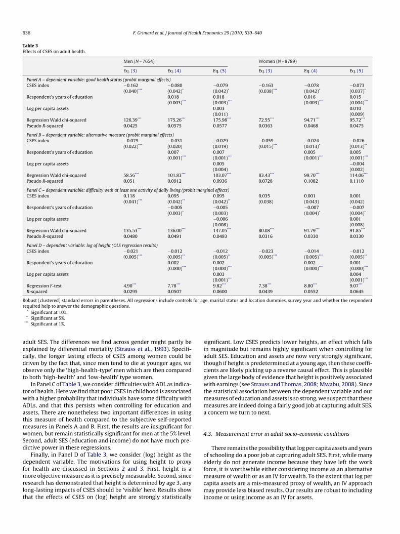
636 F. Grimard et al. / Journal of Health Economics 29 (2010) 630–640
Table 3Effects of CSES on adult health.
Men (N = 7654) Women (N = 8789)
Eq. (3) Eq. (4) Eq. (5) Eq. (3) Eq. (4) Eq. (5)
Panel A – dependent variable: good health status (probit marginal effects)CSES index −0.162 −0.080 −0.079 −0.163 −0.078 −0.073
(0.040)*** (0.042)* (0.042)* (0.038)*** (0.042)* (0.037)*
Respondent’s years of education 0.018 0.018 0.016 0.015(0.003)*** (0.003)*** (0.003)*** (0.004)***
Log per capita assets 0.003 0.010(0.011) (0.009)
Regression Wald chi-squared 126.39*** 175.26*** 175.98*** 72.55*** 94.71*** 95.72***
Pseudo R-squared 0.0425 0.0575 0.0577 0.0363 0.0468 0.0475
Panel B – dependent variable: alternative measure (probit marginal effects)CSES index −0.079 −0.031 −0.029 −0.059 −0.024 −0.026
(0.022)*** (0.020) (0.019) (0.015)*** (0.013)* (0.013)**
Respondent’s years of education 0.007 0.007 0.005 0.005(0.001)*** (0.001)*** (0.001)*** (0.001)***
Log per capita assets 0.005 −0.004(0.004) (0.002)
Regression Wald chi-squared 58.56*** 101.83*** 103.07*** 83.43*** 99.70*** 114.06***
Pseudo R-squared 0.051 0.0912 0.0936 0.0728 0.1082 0.1110
Panel C – dependent variable: difficulty with at least one activity of daily living (probit marginal effects)CSES index 0.118 0.095 0.095 0.035 0.001 0.001
(0.041)*** (0.042)** (0.042)** (0.038) (0.043) (0.042)Respondent’s years of education −0.005 −0.005 −0.007 −0.007
(0.003)* (0.003) (0.004)* (0.004)*
Log per capita assets −0.006 0.001(0.008) (0.008)
Regression Wald chi-squared 135.53*** 136.00*** 147.05*** 80.08*** 91.79*** 91.85***
Pseudo R-squared 0.0480 0.0491 0.0493 0.0316 0.0330 0.0330
Panel D – dependent variable: log of height (OLS regression results)CSES index −0.021 −0.012 −0.012 −0.023 −0.014 −0.012
(0.005)*** (0.005)** (0.005)** (0.005)*** (0.005)*** (0.005)**
Respondent’s years of education 0.002 0.002 0.002 0.001(0.000)*** (0.000)*** (0.000)*** (0.000)***
Log per capita assets 0.003 0.004(0.001)*** (0.001)***
Regression F-test 4.90*** 7.78*** 9.82*** 7.38*** 8.80*** 9.07***
R-squared 0.0295 0.0507 0.0600 0.0439 0.0552 0.0645
Robust (clustered) standard errors in parentheses. All regressions include controls for age, marital status and location dummies, survey year and whether the respondentr
aecdot
twAatmwSd
dfmrlt
siatcgwtmma
4
oe
equired help to answer the demographic questions.* Significant at 10%.
** Significant at 5%.*** Significant at 1%.
dult SES. The differences we find across gender might partly bexplained by differential mortality (Strauss et al., 1993). Specifi-ally, the longer lasting effects of CSES among women could beriven by the fact that, since men tend to die at younger ages, webserve only the ‘high-health-type’ men which are then comparedo both ‘high-health’ and ‘low-health’ type women.
In Panel C of Table 3, we consider difficulties with ADL as indica-or of health. Here we find that poor CSES in childhood is associatedith a higher probability that individuals have some difficulty withDLs, and that this persists when controlling for education andssets. There are nonetheless two important differences in usinghis measure of health compared to the subjective self-reported
easures in Panels A and B. First, the results are insignificant foromen, but remain statistically significant for men at the 5% level.
econd, adult SES (education and income) do not have much pre-ictive power in these regressions.
Finally, in Panel D of Table 3, we consider (log) height as theependent variable. The motivations for using height to proxy
or health are discussed in Sections 2 and 3. First, height is aore objective measure as it is precisely measurable. Second, sinceesearch has demonstrated that height is determined by age 3, anyong-lasting impacts of CSES should be ‘visible’ here. Results showhat the effects of CSES on (log) height are strongly statistically
fmcmi
ignificant. Low CSES predicts lower heights, an effect which fallsn magnitude but remains highly significant when controlling fordult SES. Education and assets are now very strongly significant,hough if height is predetermined at a young age, then these coeffi-ients are likely picking up a reverse causal effect. This is plausibleiven the large body of evidence that height is positively associatedith earnings (see Strauss and Thomas, 2008; Mwabu, 2008). Since
he statistical association between the dependent variable and oureasures of education and assets is so strong, we suspect that theseeasures are indeed doing a fairly good job at capturing adult SES,concern we turn to next.
.3. Measurement error in adult socio-economic conditions
There remains the possibility that log per capita assets and yearsf schooling do a poor job at capturing adult SES. First, while manylderly do not generate income because they have left the work
orce, it is worthwhile either considering income as an alternativeeasure of wealth or as an IV for wealth. To the extent that log perapita assets are a mis-measured proxy of wealth, an IV approachay provide less biased results. Our results are robust to including
ncome or using income as an IV for assets.
alth Economics 29 (2010) 630–640 637
ettwa
fmtsbtaCde
4
rimsMbsedpcp
tabMcFu
cw1cub
w
twpyo
iassa
nd
.
Mai
nm
easu
re(p
robi
tm
argi
nal
effe
ct)
Alt
.hea
lth
mea
sure
(pro
bit
mar
gin
alef
fect
)
Dif
ficu
lty
wit
hat
leas
ton
eA
DL
(pro
bit
mar
gin
alef
fect
)
log
Hei
ght
(OLS
)M
ain
mea
sure
(pro
bit
mar
gin
alef
fect
)
Alt
.hea
lth
mea
sure
(pro
bit
mar
gin
alef
fect
)
Dif
ficu
lty
wit
hat
leas
ton
eA
DL
(pro
bit
mar
gin
alef
fect
)
log
Hei
ght
(OLS
)
−0.0
38−0
.013
0.09
2−0
.007
−0.0
75−0
.022
0.00
5−0
.014
(0.0
47)
(0.0
18)
(0.0
46)**
(0.0
05)
(0.0
45)*
(0.0
14)*
(0.0
47)
(0.0
05)**
*
0.01
30.
004
−0.0
050.
001
0.01
40.
004
−0.0
080.
001
(0.0
04)**
*(0
.002
)***
(0.0
04)
(0.0
00)**
(0.0
04)**
*(0
.001
)***
(0.0
04)*
(0.0
00)**
0.00
40.
005
−0.0
070.
003
0.01
0−0
.004
−0.0
010.
004
(0.0
09)
(0.0
04)
(0.0
09)
(0.0
01)**
*(0
.009
)(0
.002
)*(0
.009
)(0
.001
)***
0.04
60.
006
−0.0
140.
014
−0.0
16−0
.001
−0.0
140.
008
(0.0
58)
(0.0
18)
(0.0
52)
(0.0
05)**
*(0
.040
)(0
.010
)(0
.044
)(0
.005
)0.
056
0.01
70.
049
0.00
40.
079
0.02
3−0
.057
−0.0
01(0
.051
)(0
.021
)(0
.046
)(0
.005
)(0
.041
)**(0
.012
)**(0
.042
)(0
.005
)0.
037
0.00
8−0
.028
−0.0
03−0
.043
−0.0
070.
021
−0.0
02(0
.030
)(0
.012
)(0
.032
)(0
.004
)(0
.027
)(0
.006
)(0
.030
)(0
.003
)65
1765
1865
1456
3474
2574
2874
2452
8316
4.11
***
117.
79**
*13
7.99
***
[6.8
0*** ]
123.
90**
*11
8.34
***
108.
07**
*[5
.33**
* ]0.
0631
0.09
990.
0514
[0.0
743]
0.05
680.
1311
0.04
08[0
.072
8]20
.86**
13.1
74.
273.
30**
*11
.16
15.3
3*13
.78
0.99
sin
clu
de
con
trol
sfo
rag
e,m
arit
alst
atu
san
dlo
cati
ond
um
mie
s,su
rvey
year
and
wh
eth
erth
ere
spon
den
tre
quir
edh
elp
toan
swer
the
dem
ogra
ph
icqu
esti
ons,
F. Grimard et al. / Journal of He
Second, years of schooling may be an inadequate measure ofducation. We check our results using the highest level of educa-ion attained and include years of education squared. Both of theseechniques allow for the non-linearity of the effect of educationhich is ignored by simply using years of schooling. Our results
re robust to these considerations.Finally, it is possible that income and education alone do not
ully account for adult socio-economic conditions. We utilize aodule in the MHAS to capture an individual’s relative social posi-
ion. Specifically, we consider the respondents’ position on theocial ladder in their neighbourhood and country.7 In addition toeing a proxy for socio-economic status, there is scientific evidencehat relative rank can impact health by leading to both physicalnd physiological stressors (Sapolsky, 2004; Marmot et al., 2001;ohen, 1999). Including either of these measures in the regressionoes little to change the fact that CSES has persistent effects onlderly health.8,9
.4. Endogeneity of CSES
The results in Table 3 are based on the assumption that theeduced form relationship between health during old age and CSESs free from bias. Many recent papers use such a reduced form,
ost of which relate to the critical-period programming hypothe-is (Maccini and Yang, 2009; Oreopoulos et al., 2008; Currie andoretti, 2007; Almond et al., 2005). These papers have credi-
le sources of exogenous variation at birth that support such apecification–they use either exogenous variation in weather toxplain birth or early infancy outcomes, or exploit twin and siblingifferences in birth weight. Almond et al. (2005) warn against inter-reting birth outcomes on later health outcomes as causal withoutontrolling for potential common third factors such as genetics orarental SES.
This line of research calls into question the results found in Sec-ion 4.1 since we are not able to find plausible exogenous variationss the literature cited above. While in principle it would be feasi-le to link MHAS individuals to weather variations at birth as inaccini and Yang (2009), the public release files do not include
urrent geographic location, let alone geographic location at birth.urthermore, the MHAS is not a twin or siblings study, so we arenable to control for third factors such as genetics in this way.
However, the structure of the MHAS allows us to investigate thisausal issue using the SES of the respondents’ parents. Respondentsere asked about their father’s (or guardian’s) occupation at age
0 (e.g. agriculture, construction, service, etc.), both parents’ edu-
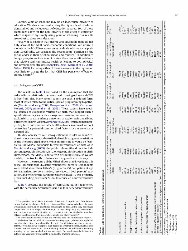
ation, and whether the parental residence at age 10 was primarilyrban. Including parental SES should reduce an omitted variablesias.Table 4 presents the results of estimating Eq. (5) augmentedith the parental SES variables, using all four dependent variables
7 The question reads: “Here is a ladder. There are 10 steps in total from bottomo top. Look at this ladder. At the very top you’ll find people who have the mosteight on decisions, or on how things are going to be done. At the very bottom areeople with the least weight in decisions, or on how things are going to be done. Ifou consider your present situation and compare it with that of all other membersf [your neighbourhood/Mexico], where would you place yourself?”8 All of our results for this section are available from the authors upon request.9 We believe that our adult SES measures are doing a good job at capturing health
nvestment decisions throughout the life-cycle. The MHAS provides one more vari-ble that would allow us to capture such decisions: whether the individual has evermoked. We re-ran our main tables including whether the individual is currentlymoking or has once smoked but has since quit. Our results (available from theuthors upon request) are robust to including the smoking variables. Ta
ble
4Ef
fect
sof
CSE
Son
adu
lth
ealt
h,c
ontr
olli
ng
for
par
enta
lbac
kgro
u
CSE
Sin
dex
Res
pon
den
t’s
year
sof
edu
cati
on
Log
per
cap
ita
asse
ts
Mot
her
had
com
ple
ted
pri
mar
ysc
hoo
l
Fath
erh
adco
mp
lete
dp
rim
ary
sch
ool
Pare
nta
lres
iden
cew
asp
rim
aril
yu
rban
N Reg
ress
ion
Wal
dch
i-sq
uar
edte
st[r
egre
ssio
nF-
test
]Ps
eud
oR
-squ
ared
[R-s
quar
ed]
Join
tF-
test
ofsi
gnifi
can
ceof
par
enta
lbac
kgro
un
dva
riab
les
Rob
ust
(clu
ster
ed)
stan
dar
der
rors
inp
aren
thes
es.A
llre
gres
sion
and
du
mm
ies
for
fath
er’s
occu
pat
ion
.*
Sign
ifica
nt
at10
%.
**Si
gnifi
can
tat
5%.
***
Sign
ifica
nt
at1%
.
638 F. Grimard et al. / Journal of Health Economics 29 (2010) 630–640
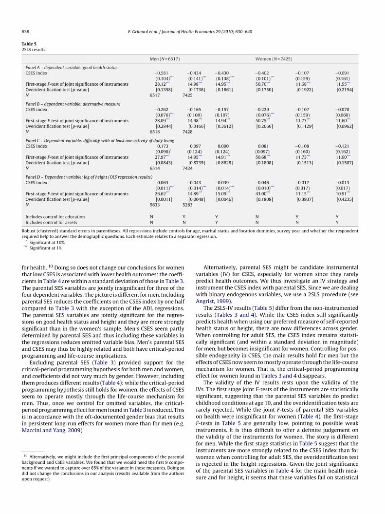
Table 52SLS results.
Men (N = 6517) Women (N = 7425)
Panel A – dependent variable: good health statusCSES index −0.581 −0.434 −0.430 −0.402 −0.107 −0.091
(0.104)*** (0.141)*** (0.138)*** (0.101)*** (0.159) (0.161)First-stage F-test of joint significance of instruments 28.12*** 14.98*** 14.95*** 50.70*** 11.68*** 11.55***
Overidentification test [p-value] [0.1358] [0.1736] [0.1861] [0.1750] [0.1922] [0.2194]N 6517 7425
Panel B – dependent variable: alternative measureCSES index −0.262 −0.165 −0.157 −0.229 −0.107 −0.070
(0.076)*** (0.108) (0.107) (0.076)*** (0.159) (0.060)First-stage F-test of joint significance of instruments 28.09*** 14.98*** 14.94*** 50.75*** 11.73*** 11.60***
Overidentification test [p-value] [0.2844] [0.3166] [0.3612] [0.2066] [0.1129] [0.0962]N 6518 7428
Panel C – Dependent variable: difficulty with at least one activity of daily livingCSES index 0.173 0.097 0.090 0.081 −0.108 −0.121
(0.096)* (0.124) (0.124) (0.097) (0.160) (0.162)First-stage F-test of joint significance of instruments 27.97*** 14.95*** 14.91*** 50.68*** 11.73*** 11.60***
Overidentification test [p-value] [0.8843] [0.8735] [0.8628] [0.1808] [0.1513] [0.1507]N 6514 7424
Panel D – Dependent variable: log of height (OLS regression results)CSES index −0.063 −0.043 −0.039 −0.046 −0.017 −0.013
(0.011)*** (0.014)*** (0.014)*** (0.010)*** (0.017) (0.017)First-stage F-test of joint significance of instruments 26.62*** 14.89*** 15.09*** 43.00*** 11.15*** 10.91***
Overidentification test [p-value] [0.0011] [0.0048] [0.0046] [0.1808] [0.3937] [0.4235]N 5633 5283
Includes control for education N Y Y N Y YIncludes control for assets N N Y N N Y
Robust (clustered) standard errors in parentheses. All regressions include controls for age, marital status and location dummies, survey year and whether the respondentr rate r
ftcTfpcTssdtap
catpsmpiiM
bndu
vpiwA
rphWcfseme
Isc
equired help to answer the demographic questions. Each estimate relates to a sepa* Significant at 10%.
*** Significant at 1%.
or health. 10 Doing so does not change our conclusions for womenhat low CSES is associated with lower health outcomes: the coeffi-ients in Table 4 are within a standard deviation of those in Table 3.he parental SES variables are jointly insignificant for three of theour dependent variables. The picture is different for men. Includingarental SES reduces the coefficients on the CSES index by one halfompared to Table 3 with the exception of the ADL regressions.he parental SES variables are jointly significant for the regres-ions on good health status and height and they are more stronglyignificant than in the women’s sample. Men’s CSES seem partlyetermined by parental SES and thus including these variables inhe regressions reduces omitted variable bias. Men’s parental SESnd CSES may thus be highly related and both have critical-periodrogramming and life-course implications.
Excluding parental SES (Table 3) provided support for theritical-period programming hypothesis for both men and women,nd coefficients did not vary much by gender. However, includinghem produces different results (Table 4): while the critical-periodrogramming hypothesis still holds for women, the effects of CSESeem to operate mostly through the life-course mechanism foren. Thus, once we control for omitted variables, the critical-
eriod programming effect for men found in Table 3 is reduced. Thiss in accordance with the oft-documented gender bias that resultsn persistent long-run effects for women more than for men (e.g.
accini and Yang, 2009).
10 Alternatively, we might include the first principal components of the parentalackground and CSES variables. We found that we would need the first 9 compo-ents if we wanted to capture over 85% of the variance in these measures. Doing soid not change the conclusions in our analysis (results available from the authorspon request).
roFitfiwios
egression.
Alternatively, parental SES might be candidate instrumentalariables (IV) for CSES, especially for women since they rarelyredict health outcomes. We thus investigate an IV strategy and
nstrument the CSES index with parental SES. Since we are dealingith binary endogenous variables, we use a 2SLS procedure (seengrist, 1999).
The 2SLS-IV results (Table 5) differ from the non-instrumentedesults (Tables 3 and 4). While the CSES index still significantlyredicts health when using our preferred measure of self-reportedealth status or height, there are now differences across gender.hen controlling for adult SES, the CSES index remains statisti-
ally significant (and within a standard deviation in magnitude)or men, but becomes insignificant for women. Controlling for pos-ible endogeneity in CSES, the main results hold for men but theffects of CSES now seem to mostly operate through the life-courseechanism for women. That is, the critical-period programming
ffect for women found in Tables 3 and 4 disappears.The validity of the IV results rests upon the validity of the
Vs. The first stage joint F-tests of the instruments are statisticallyignificant, suggesting that the parental SES variables do predicthildhood conditions at age 10, and the overidentification tests arearely rejected. While the joint F-tests of parental SES variablesn health were insignificant for women (Table 4), the first-stage-tests in Table 5 are generally low, pointing to possible weaknstruments. It is thus difficult to offer a definite judgement onhe validity of the instruments for women. The story is differentor men. While the first stage statistics in Table 5 suggest that the
nstruments are more strongly related to the CSES index than foromen when controlling for adult SES, the overidentification tests rejected in the height regressions. Given the joint significancef the parental SES variables in Table 4 for the main health mea-ure and for height, it seems that these variables fail on statistical
alth E
ctffiwhrq
fpetSmfmStpbausatht
fpib(mbania
5
twftoa
oehawiai
od
cocttss
fhtntl(lfiMaogrra
R
A
A
A
A
A
B
B
B
B
B
B
C
C
C
C
C
F. Grimard et al. / Journal of He
riteria. Thus, it is not clear to what extent the IV procedure is statis-ically valid for men in the case of our preferred health measure oror height, even though the overidentification test is not rejectedor the former. For the alternative health measure and ADLs, thenstruments satisfy the statistical criteria (though remain weak
hen controlling for adult SES) and the IV results for the alternativeealth measure are qualitatively similar to the non-instrumentedesults. Meanwhile, the IV results on ADL are both qualitatively anduantitatively similar to the non-instrumented results.
Statistically, the IV results do not offer conclusive evidence inavour or against the relative importance of the critical-periodrogramming versus life-course mechanisms. However, the differ-nces across gender do suggest some differences in the channelshrough which current health is affected by CSES and parental SES.pecifically, parental SES predict health above and beyond CSES foren but not for women and they are weaker instruments for CSES
or women than for men. Several explanations may be offered. First,en and women may have different recollections about parental
ES, and so measurement error may vary across gender in wayshat confound the IV analysis. Second, the relationship betweenarental SES and CSES might somehow be different for girls andoys. Third, the relationship between health and parental SES mightlso vary by gender. If gender bias was an issue when the individ-als in our sample were born, son preferring rules might explainome of these differences. Finally, there could be other unobserv-ble (e.g. genetic) differences across men and women that comeo play in the relationship between parental SES, CSES and adultealth. Either way, the MHAS does not provide sufficient informa-ion to explore these differences more fully.
Regardless of the statistical criteria, these instruments may alsoail on economic grounds: it is impossible to reject the theoreticalossibility that parental background has a direct effect on health
n old age. For instance, parental SES, CSES and health could alsoe jointly determined by a ‘third factor’ such as genetics (G in Eq.2)). The error term of Eq. (5) would then contain G and the esti-
ated coefficients in our tables would suffer from omitted variableias to the extent that parental SES are related to G. Unfortunately,lthough we have tried to minimize this bias, the available data doot allow us to fully reject the possibility that a factor such as genet-
cs may explain the significant effect of childhood circumstances ondult health.11
. Discussion
We find long-lasting effects of childhood SES on health amonghe elderly in Mexico. The effect is particularly persistent foromen. While these results are consistent with growing evidence
rom developed and developing countries, our results contributeo this body of knowledge by finding evidence among a previ-usly under-researched yet growing demographic: the elderly indeveloping country.
We check for robustness of our results to several limitations ofur empirical strategy. First, we take into account measurementrror in the dependent variable by alternative proxies for goodealth. Second, we consider the possibility that our measures ofdult socio-economic conditions are measured with error. Third,
hile the data do not allow us to formally control for endogeneityn childhood circumstances, we consider a two stage least squarespproach to deal with endogeneity using parental backgroundnformation. In all cases, we find persistent effects of childhood
11 It should be noted that other existing studies (Maccini and Yang, 2009; Ore-poulos et al., 2007; Currie and Moretti, 2007; Almond et al., 2005) could not fullyismiss that possibility either.
C
C
E
G
conomics 29 (2010) 630–640 639
ircumstances on health of the elderly. While it is still possible thatur results are due to measurement error in adult socio-economiconditions (which would favour the life-course model only) or thathey are due to an unobserved factor such as genetics (which wouldhen invalidate both life-course and critical programming hypothe-es), it would appear that the critical programming hypothesishould not be dismissed as a factor explaining these effects.
If so, our results have several implications for policy. First, theact that childhood circumstances have a long-lasting effect onealth of the elderly, which persists when controlling for educa-ion and wealth, suggests that cash transfers to the elderly mayot completely counter the negative effects from poverty a life-ime ago. Second, because conditions during childhood are so longived and independent of adult SES such as education and wealthlending support to the critical-period programming model), theong-term benefits such as improved health in old age should beactored into the cost–benefit analysis of child welfare policy. Fornstance, our results imply that conditional cash transfers such as
exico’s Oportunidades can have effects on recipients’ health in oldge even beyond the intended effects on schooling and child healthutcomes. Third, as developing countries face their dual demo-raphic and epidemiological transitions, and as childhood povertyates fall, policy makers should be forward-looking in allocatingesources to a growing, aging cohort, whose morbidity tends to bessociated with relatively more expensive chronic diseases.
eferences
kresh, R., Verwimp, P., Bundervoet, T., forthcoming. Civil war, crop failure, and thehealth status of young children. Economic Development and Cultural Change.
lmond, D., 2006. Is the 1918 influenza pandemic over? Long-term effects of inutero influenza exposure in the post-1940 U.S. population. Journal of PoliticalEconomy 114 (4), 672–712.
lmond, D., Chay, K., Lee, D., 2005. The costs of low birth weight. Quarterly Journalof Economics 102 (3), 1031–1083.
ngrist, J., 1999. Estimation of limited dependent variable models with dummyendogenous regressors: simple strategies for empirical practice. Journal of Busi-ness Economics and Statistics 19 (1), 2–28.
storga, P., Berges, A., Fitzgerald, V., 2005. The standard of living in Latin Americaduring the twentieth century. Economic History Review 58 (4), 765–796.
aker, M., Stabile, M., Deri, C., 2004. What do self-reported, objective, health mea-sures of health measure? Journal of Human Resources 39 (4), 1067–1193.
arker, D.J.P., 1998. Mothers, Babies and Health in Later Life, 2nd ed. Churchill Liv-ingstone, Edinburgh.
arker, D.J.P., Eriksson, J.G., Forsén, T., Osmond, C., 2002. Fetal origins of adultdisease: strength of effects and biological basis. International Journal of Epi-demiology 31 (6), 1235–1239.
arro, R., Ursua, J., 2008. Macroeconomic Crises since 1870. NBER Working Paper #W13940.
en-Slomo, Y., Kuh, D., 2002. A life course approach to chronic disease epidemiology:conceptual models, empirical challenges and interdisciplinary perspectives.International Journal of Epidemiology 31 (2), 285–293.
uckley, N.J., Denton, F.T., Robb, A.L., Spencer, B.G., 2004. The transition from goodto poor health: an econometric study of the older population. Journal of HealthEconomics 23 (5), 1013–1034.
ase, A., Lubotsky, D., Paxson, C., 2002. Economic status and health in childhood:the origins of the gradient. American Economic Review 92 (5), 1308–1334.
ase, A., Fertig, A., Paxson, C., 2005. The lasting impact of childhood health andcircumstance. Journal of Health Economics 24 (2), 265–289.
ohen, S., 1999. Social status and susceptibility to respiratory infections. Annals ofthe New York Academy of Sciences 896, 246–253.
rossley, T., Kennedy, S., 2002. The reliability of self-assessed health status. Journalof Health Economics 21 (4), 643–658.
urrie, J., Moretti, E., 2007. Biology as destiny? Short- and long-run determinants ofintergenerational transmission of birth weight. Journal of Labor Economics 25(2), 231–263.
urrie, J., Stabile, M., 2003. Socio-economic status and health: why is the relationshipstronger for older children? American Economic Review 93 (5), 1813–1823.
urrie, J., Hyson, R., 1999. Is the impact of health shocks cushioned by socio-economic status? The case of low birth weight. American Economic Review
Papers and Proceedings 89 (2), 246–250.lo, I.T., Preston, S.H., 1992. Effects of early-life conditions on adult mortality: areview. Population Index 58 (2), 186–212.
lewwe, P., Miguel, E., 2008. The impact of child health and nutrition on educa-tion in less developed countries. In: Schutlz, T.P., Strauss, J. (Eds.), Handbook ofDevelopment Economics, Vol. 4. North-Holland, Amsterdam.
6 alth E
G
G
K
L
L
M
M
M
M
O
R
S
S
40 F. Grimard et al. / Journal of He
raham, H., 2002. Building an inter-disciplinary science of health inequalities: theexample of lifecourse research. Social Science and Medicine 55 (11), 2005–2016.
rossman, M., 1972. On the concept of health capital and the demand for health.Journal of Political Economy 80 (2), 223–255.
uh, D.J., Wadsworth, M.E., 1993. Physical health status at 36 years in a Britishnational birth cohort. Social Science and Medicine 37 (7), 905–916.
ópez-Alonso, M., Porras Condey, R., 2003. The ups and downs of Mexican economicgrowth: the biological standard of living and inequality, 1870–1950. Economicsand Human Biology 1 (2), 169–186.
ópez-Alonso, M., 2007. Growth with Inequality: living standards in Mexico,1850–1950. Journal of Latin American Studies 39, 81–105.
accini, S., Yang, D., 2009. Under the weather: health, schooling, and eco-nomic consequences of early-life rainfall. American Economic Review 99 (3),1006–1026.
armot, M., Shipley, M., Brunner, E., Hemingway, H., 2001. Relative contribution ofearly life and adult socioeconomic factors to adult morbidity in the Whitehall IIstudy. Journal of Epidemiology and Community Health 55, 301–307.
ete, C., 2005. Predictors of elderly mortality: health status, socio-economic char-acteristics and social determinants of health. Health Economics 14 (2), 135–148.
S
V
conomics 29 (2010) 630–640
wabu, G., 2008. Health economics for low-income countries. In: Schutlz, T.P.,Strauss, J. (Eds.), Handbook of Development Economics, Vol. 4. North-Holland,Amsterdam.
reopoulos, P., Stabile, M., Walld, R., Roos, L., 2008. Short-, medium-, and long-term consequences of poor infant health. Journal of Human Resources 43 (1),138–188.
oy, K, Chaudhuri, A., 2008. Influence of socioeconomic status, wealth and financialempowerment on gender differences in health and healthcare utilization in laterlife: evidence from India. Social Science and Medicine 66, 1951–1962.
apolsky, R.M., 2004. Social status and health in humans and other animals. AnnualReview of Anthropology 33, 393–418.
trauss, J., Gertler, P., Rahman, O., Fox, K., 1993. Gender and life-cycle differentialsin the patterns and determinants of adult health. Journal of Human Resources28 (4), 791–837.
trauss, J., Thomas, D., 2008. Health over the life-course. In: Schutlz, T.P., Strauss,J. (Eds.), Handbook of Development Economics, Vol. 4. North-Holland, Amster-dam.
an Ourti, T., 2003. Socio-economic inequality in ill-health amongst the elderly:should one use current or permanent income. Journal of Health Economics 22(2), 219–241.