headaches in hodge theoryw3.impa.br/~hossein/myarticles/headaches.pdf · hossein movasati headaches...

Hossein Movasati

Headaches in Hodge theory

The text is a collection of my thoughts and correspondences and it is not intended for publication.

July 23, 2020

Publisher

Chapter 1Infinitesimal deformations

The following notes are written after many email exchanges with P. Deligne inNovermber 2018. The main objective of the notes is two folded. First, we wouldlike rewrite the results of [Mov19a, Chapter 18] using the formalism of infinitesi-mal schemes over a field k of characteristic zero. Second, to reproduce some of P.Deligne’s questions and suggestions.

1.1 Deformation over infinitesimal schemes

Let T be a reduced and smooth scheme over a field k of chararacteristic 0, 0 ∈ T bea k-rational point of T and S → T be a possibly non-reduced sub scheme of T. Forinstance, T := Spec(k[t1, t2, . . . , ts]) and

S := Spec(k[t1, t2, . . . , ts]/〈tN+1

1 , · · · , tN+1s , f1, f2, · · · 〉

)= Spec

(k[t]/〈tN+1, f 〉

)(1.1)

where f1, f2, . . . is a set of polynomials in k[t]. We take a projective smooth schemeXT over T and denote by X/S the induced scheme. In general we may work with

Definition 1.1 Let M be the maximal ideal of OS,0. We call

SN := Spec(OS,0

/M N+1

)(1.2)

the N-th infinitesimal scheme of S at 0. We also call the induced scheme X/S, theN-th order deformation of X0.

The fiber over 0 is denote by X0. From now on I will use X/T instead of XT/T.The relative algebraic de Rham cohomology Hm

dR(X/T) is a free OT-module of rankdimkHm

dR(X0/k). We denote the pieces of its Hodge filtration by F i =F iHmdR(X/T), i=

0,1,2, . . . ,m. We have also the Gauss-Manin connection

∇ : HmdR(X/T)→Ω

1T⊗OT

HmdR(X/T)

1

2 1 Infinitesimal deformations

In an earlier draft of this text, I worte the formalisim of Gauss-Manin connectiondirectly for S (not using the bigger space T). This was trivially false as rings like theone used in (1.1) might have elements f such that d f = 0 but f is not constant. Thisresulted in the following comment.

1.1 (P. Deligne, 20 November, 2018) You need the crystalline story, which tellsthat for X smooth (proper is not needed) over a S such as (1.1), HdR(X/S) dependsonly (up to a canonical isomorphism) on X0/Spec(C). In other words, one has acanonical isomorphism

HdR(X/S)∼= HdR(X0)⊗R (1.3)

[R being the ring of S]. In your cases, you will have S → T, T smooth, and X/Sis induced by XT/T, proper and smooth. In that case, the Gauss-Manin connectioninduces a constantification of HdR(XT/T) on a formal neighborhood of 0 ∈ T, andit induces (1.3) on S.

Now we can talk about the Gauss-Manin connection

∇ : HmdR(X/S)→Ω

1S ⊗OS Hm

dR(X/S)

and any other object related to de Rham cohomologies, such as trace map, polar-ization and cup product, as it is explained in the comments above. We take a sub-scheme Z0 of codiemsnion p := m

2 in X0/k and denote its cohomology class bycl(Z0)∈Hm(X0/k). There is a unique section s of Hm

dR(X/S) such that ∇(s) = 0 ands0 = cl(Z0). This is called the horizontal extension of cl(Z0) or a flat section of thecohomology bundle.

Definition 1.2 Let X/S and X0 be as above. The Hodge locus V X/S[Z0]

is a subschemeof S given by the conditions

∇(s) = 0, (1.4)

s ∈ Fm2 Hm

dR(X/S), (1.5)s0 = cl(Z0). (1.6)

For the reduced smooth T and X/T as above we use the notation

V ∞

[Z0]=V[Z0] :=V X/T

[Z0]

and for the N-th order deformation X/SN of X0 as in Definition 1.1 we use

V N[Z0]

:=V X/SN

[Z0]

and call it the N-th infinitesimal Hodge locus.

1.2 (P. Deligne, November 13, 2018) Note that we did not need to require that sis at each point V[Z0] an integral cohomology class-which would be a transcendentalcondition-it comes free from (1.4) and (1.6).

1.1 Deformation over infinitesimal schemes 3

Definition 1.3 We define T = TZ0 to be the algebraic subset of T coming fromCattani-Deligne-Kaplan theorem applied to the Hodge locus V[Z0] = V X/T

[Z0]. We de-

note by VZ0 ⊂ (T,0) the local analytic subset of (T,0) parametrizing flat deforma-tions of Z0. We have

VZ0 ⊂V[Z0] ⊂ TZ0

i

Definition 1.4 We say that the alternative Hodge conjecture (AHC) holds for thepair (X0,Z0) if

VZ0 =V[Z0]

as analytic varieties.

For many examples of (X0,Z0) such that AHC does not hold see [Mov19a, §18.2].

Proposition 1.1 If X/S,X0,Z0 are defined over k then V[Z0] is also defined over k.

Proof. This follows from the fact that the Gauss-Manin connection and the coho-mology class of Z0 are defined over k. ut

However, note that the condition (1.4) is mixed algebraic and holomorphic con-dition. Whereas ∇ is algebraic, its flat section s for reduced schemes is given byholomorphic functions. After passing to infinitesimal schemes we use the trunca-tion of of such series, and hence, get polynomials. The section s can be computedexplicitly once the Gauss-Manin connection is computed. In this way the equationsof the Hodge locus are hidden in (1.5) which can be written as

〈ω,s〉= 0, ∀ω ∈ Fm2 +1Hm

dR(X/S).

where

〈·, ·〉 : HmdR(X/S)×Hm

dR(X/S)→ OS(S), (s,β ) 7→ Tr(s∪β ∪θ2n−2m). (1.7)

and θ ∈ H2(X/S) is the polarization. For T reduced and smooth scheme and ω asection of Hm

dR(X/T) around 0, we know that∫δt

ω ∈ k[[t]] = ring of formal power series in t with coefficients in k (1.8)

where δt ∈Hm(Xt ,Z) is the monodromy of δ0 := [Z0] to nearby fibers, that is, periodsare formal power series (actually convergent) in t with coefficients in k. The idealof the Hodge locus V[Z0] in this case is given by

i I am not sure whether VZ0 in general exists! Duco van Straten kindly reminded me [January 14,2019] that “the requirement of flatness of a cycle is not a reasonable condition at all. Flatness isjust too special. There is the notion of families of cycles used by Barlet in analytic and by Kollarin algebraic geometry[see [Kol95], page 45-46 and [Bar75]]. It is very ugly and algebraically hardto use, but geometrically reasonable.”

4 1 Infinitesimal deformations⟨Fi

∣∣∣i = 1,2, . . . ,b⟩, Fi :=

∫δt

ωi,

where ωi’s are sections of HmdR(X/T) around 0 which form a basis of F

m2 +1Hm

dR(X/T)at each fiber near 0. For families of hypersurfaces and the Fermat variety X0, onecan give closed formulas for the coefficients of (1.10), see [Mov19a, Theorem 13.2,Theorem 18.9]. In this case, instread of [Z0] we can take any Hodge cycle and kis always an abelian extension of the cyclotomic field Q(ζd), see Deligne’s lecturemotes in [DMOS82].

Remark 1.1 Let X/T be a deformation of X0 with T smooth and reduced. Thetangent space of V X/T

[Z0]at 0 is just the first order infinitesimal Hodge locus V 1

[Z0]=

V X/T1

[Z0].

Replacing π : X→ S with π−1(V X/S[Z0]

)→V X/S[Z0]

we get the following type of families:

Definition 1.5 Let X/S be a deformation of X0 and Z0 ⊂ X0 be an algebraic cycle ofcodimension of codimension m. We say that cl(Z0) remains Hodge in S if we have(1.4), (1.5) and (1.6).

The following question was originally posed for the number of parameters equal to1 and N = 1.

1.3 (P. Deligne, November 11, 2018) In what sense should we deform Z0 into Zover S to make sure that cl(Z0) remains Hodge over S, meaning that its horizontalextension in Hm

dR(X/S), the bundle over S of relative de Rham cohomology, remainsof Hodge filtration m

2 ? I expect it suffices that for some E0 of codimension ≥ 2 inZ0, we have outside of E0 a flat extension, noted Z−E, of Z0−E0. The point is thatsuch a Z−E should give us a natural extension of cl(Z0) in

F p(HdR(X/S)) =

H p(X/S, truncated relative dR complex starting at Ω p put in cohomological degree 0 ).

1.4 (P. Deligne, November 15, 2018) I still think it might be useful to better un-derstand, over an infinitesimal basis, in which sense (weaker than flat deformationas a subscheme) a cycle should be deformed to ensure that its class remains Hodgeby some (infinitesimal, for instance first order) deformation: if the Fi are the localequations you use for the Hodge locus, and if an intersection of dFi = 0 is biggerthan expected, but if this can be explained by deformations in a weak sense, then itis no evidence for an Hodge locus of dimension bigger than expected.

1.5 (P. Deligne, November 20, 2018) Barlet and Argeniol have tried to define fam-ily of Chow cycles in the Xs of X/S, I do not remember what they could do, nor afamily of Chow cycles in their sense give what one wants. One idea they use is thatsuch [Chow cycle] to be defined

Z → X↓S

http://www.iecl.univ-lorraine.fr/~Daniel.Barlet/

1.2 Main example 5

should locally, for U ⊂ X a coordinate system and U →V a smooth projection withdimV = dim(Z), Z finite over V , one should have a trace map

TrZ/V : OU → OV

with nice properties (such as, for some d, to be the degree of Z over V , and( fi)i∈I , |I|= d +1)

∑S⊂I

(−1)|S|Tr(∏i∈S

fi) = 0). (1.9)

Long ago, I had hopes that having this for one projection gives us the same for any,but Argeniol showed I was wrong.

Note that the condition (1.9) can be re written in the following way. Taking the traceof the homogenuous pieces of

d+1

∏i=1

(1− fi)

and still summing them up, we get 1. We have assumed that Tr(1) = 1 and note thatTr is not necessarily additive. For more discussion on this topic see 4.6. I do nothave any intuition regarding this comment.

1.2 Main example

Let T be the parameter space of smooth hypersurfaces of degree d and dimensionn. For

−1≤ m≤ n2−2

let Tm be the parameter space of hypersurfaces X containing two linear P n2 and P n

2

withP

n2 ∩ P

n2 = Pm, (1.10)

that is, their intersection is of dimension m.

Proposition 1.2 Any deformation (Xt ,Zt) of the pair (X ,P n2 + P n

2 ) will give us a

flat deformation of Z0 = P n2 + P n

2 and Zt = Pn2t + P

n2t with P

n2t ∩ P

n2t = Pm

t .

Proof. A pair (X ,P n2 + P n

2 ) with (1.10) cannot be deformed into another pair withdifferent m. This is because the topological intersection of these two cycles insideX is given by the formula:

Pn2 · P

n2 =

1− (−d +1)m+1

d. (1.11)

see [Mov19a, Section 17.6]. ut


Note that the deformation of the pair (P n2 , P n

2 ) with (1.10) is in the oppositedirection: It can be deformed into another pair with an arbitrary m and the genericdeformation will produce a pair with m=−1. It must be easy to prove the following:

Proposition 1.3 Let X → T be a morphism of algebraic varieties over k such thatits generic fiber is PN ∪Pm PN and its fiber over 0 is PN ∪Pm PN . If m 6= m then X/Sis not flat over 0.

The conclusion is that a falt deformation (in our case smooth which is stronger) of avariety X0, forces either an algebraic cycle Z0 ⊂ X0 to disappear or to be deformedflat. It might be interesting to find a counterexample to this, that is, to find a smoothX/S with an algebraic cycle Z of codimension m

2 in X/S such that the only non-flatfiber of Z is the central fiber Z0. This is the topic of §4.6.

For some computer assisted proofs we will take

Pn2 :

x0−ζ2dx1 = 0,x2−ζ2dx3 = 0,x4−ζ2dx5 = 0,· · ·xn−ζ2dxn+1 = 0.

Pn2 :

x0−ζ2dx1 = 0,· · ·x2m−ζ2dx2m+1 = 0,x2m+2−ζ 3

2dx2m+3 = 0,· · ·xn−ζ 3

2dxn+1 = 0.

(1.12)

where ζ2d := e2π√−1

2d . These are linear algebraic cycles in the Fermat variety Xdn ⊂

Pn+1 given by the homogeneous polynomial xd0 + xd

1 + · · ·+ xdn+1 = 0, and satisfy

P n2 ∩ P n

2 = Pm.

1.3 First order deformation

Recall the first order infinitesimal scheme T1 ⊂ T at 0 and the corresponding first

order deformation X/T1 of X0. Recall also V 1[Z0]

:=V X/T1

[Z0]and V[Z0] :=V X/T

[Z0].

Proposition 1.4 If dimkV 1[Z0]

= dim(VZ0) then V[Z0] = VZ0 , that is, AHC holds for(X0,Z0). Moreover, V[Z0] is smooth and reduced.

Proof. The Zariski tangent space of V[Z0] at 0 is V 1[Z0]

and VZ0 ⊂V[Z0]. ut

The following examples satisfies the hypothesis of Proposition 1.4. We have takenX/T to be the full family of smooth hypersurfaces.

1. Complete intersection algebraic cycles after [Dan14a, MV19]: Assume that n≥ 2is even and f ∈ C[x]d is of the following format:

f = f1 f n2+2+ f2 f n

2+3+ · · ·+ f n2+1 fn+2, fi ∈C[x]di , f n

2+1+i ∈C[x]d−di , (1.13)

where 1≤ di < d, i = 1,2, . . . , n2 +1 is a sequence of natural numbers. Let X0 ⊂

Pn+1 be the hypersurface given by f = 0 and Z0 ⊂ X0 be the algebraic cycle given

1.4 Second order deformations 7

by f1 = f2 = · · ·= f n2+1 = 0. We call Z0 a complete intersection algebraic cycle

in X0.2. Sum of two linear cycles [MV19, Mov19a]: Let X0 be a smooth hypersurface of

degree d and dimension n which contains two linear P n2 and P n

2 with P n2 ∩ P n

2 =Pm. For a generic choice of X0

ii The algebraic cycle Z0 := rP n2 + rP n

2 , r, r 6= 0with (n,d,m) in the list

(2,d,−1), 5≤ d ≤ 14,(4,4,−1),(4,5,−1),(4,6,−1),(4,5,0),(4,6,0),(6,3,−1),(6,4,−1),(6,4,0),(8,3,−1),(8,3,0),(10,3,−1),(10,3,0),(10,3,1),

In [Vil20] this has been generalized to cases:

d < (d−2)(n2−m) (1.14)

For instance, for all m≤ n2 −2 and d ≥ 5.

1.4 Second order deformations

Remark 1.2 In the following when we talk about Hilbert schemes, we actuallymean a connected open subset of it, over which the corresponding family is flat.

Let us consider an irreducible algebraic cycle Za in Xa and assume that in theflag Hilbert scheme Hilb(Xa,Za) it has a degeneration (X0,Z0) in which X0 is stillsmooth but Z0 = P0 + P0, where P0 and P0 are two irreducible algberaic cycles. Itfollows that the codimension of P0 ∩ P0 in both P0 and P0 is one. Assume that forthree algebraic cycles C = Z0,P0, P0 the following property holds: the tangent spaceof V[C] at the point 0 ∈ Hilb(X0) corresponding to X0 is equal to the dimension ofthe image of

Hilb(X0,C)→ T := Hilb(X0).

This implies that the alternative Hodge conjecture (see [Mov19a, Conjecture 18.2])is true for the pairs (X0,Z0), (X0,P0),(X0, P0).

Conjecture 1.1 Assume that

dimFm2 +1Hm

dR(X0)> 1. (1.15)

The second infinitesimal Hodge locus V 2r[P0]+r[P0]

for r, r ∈Z,r, r 6= 0,r 6= r is singularat 0, and hence, the Hodge locus Vr[P0]+r[P0]

is singular at 0. The condition (1.15) is

ii Here, generic means in some Zariski open subset of the algebraic subset of T parametrizing thoseX0.


needed, otherwise all Hodge loci would be either the whole space or of codimensionone.

Note that ‘singular’ in the above statement is used in the scheme theoretic context.If the underlying analytic variety of Vr[P0]+r[P0]

is smooth then the above statementsays that it is not reduced. Note also that in Conjecture 1.1, r = r is excluded as(X0,Z0), Z0 = P0 + P0) has a larger deformation space in which the deformed alge-braic cycle Zt is irreducible.

Theorem 1.6 ( [Mov19a], Theorem 18.3, part 1) Conjecture 1.1 is true for theFermat hypersurface X0 of degree d and dimension n and Z0 = P n

2 + P n2 with (1.12)

and in the following cases: For all r, r ∈ Z, 1 ≤ |r| ≤ |r| ≤ 10, r 6= r and (n,d) inthe list

(2,d), 5≤ d ≤ 9, (1.16)(4,4),(4,5),(6,3),(8,3) (1.17)

One might claim that the underlying analytic variety of Vr[P0]+r[P0], r, r 6= 0,r 6=

r is V[P0] ∩V[P0]. However, this is stronger than Conjecture 1.1. The dimension of

V[P0]∩V[P0]is less than the dimension of the Zariski tangent space of Vr[P0]+r[P0]

at 0,and when the differenc is only one, this stronger statement is true. This is the case,for instance, for Example 4.6 and Example 4.7. The second order approximation ofHodge loci is also formulated by Maclean [Mac05, Theorem 7], see also Theorem8 for some applications in the case of quintic surfaces with two disjoint lines, thatis, (n,d,m) = (2,5,−1).

1.5 Degeneration of algebraic cycles

Let X be a smooth projective variety and Z = ∑ri=1 niZi, ni ∈ Z be an algebraic

cycle in X , with Zi an irreducible subvariety of codimension n2 in X . The following

definition is done using analytic deformations and it would not be hard to state it inthe algebraic context.

Definition 1.7 We say that Z = ∑ri=1 niZi, ni ∈ Z is semi-irreducible if there is a

smooth analytic variety X , an irreducible subvariety Z ⊂X of codimension n2

(possibly singular), a holomorphic map f : X → (C,0) such that

1. f is smooth and proper over (C,0) with X as a fiber over 0. Therefore, all thefibers Xt of f are C∞ isomorphic to X .

2. The fiber Zt of f |Z over t 6= 0 is irreducible and Z0 = ∪ri=1Zi.

3. The homological cycle [Z] := ∑ri=1 ni[Zi] ∈ Hn(X ,Z) is the monodromy of [Zt ] ∈

Hn(Xt ,Z).

1.6 (P. Deligne 15 November, 2018) [In Definition 1.7] 3. is strangely weak: Don’tyou want the fiber, as an algebraic cycle, to be ∑niZi? What 3. requires is weakerwhen the cohomology classes of the Zi are not linearly independent.

1.6 Equations for Hodge loci 9

The above comment is absolutely correct. One might regard Zi as a scheme deter-mined by its sheaf of ideals Ii, and therefore, niZi has the sheaf of ideals I ni

i .For this we assume that ni ∈ N. In this way we are talking about degeneration ofschemes. Doing in this way one has to prove that

Proposition 1.5 The cohomology class cl(Zt) is flat, that is, ∇(cl(Zt)) = 0.

The following examples might help to define the general concept of deformation ofalgebraic cycles.

1.7 (P. Deligne, November 7, 2018) Take a smooth divisor Z on Y , and blow upmany points of Y on Z to get X . As cycle C take the pure transform of Z. If we deformX by moving in Y the points to be blown up, the cycle is usually not able to follow.Here it matters what is to be called ‘deformation’: C = (C+exceptional divisors)−(exceptional divisors), and both can be deformed.

1.6 Equations for Hodge loci

Let X→ T be a family of smooth projective varieties over k. Let Z0 ⊂ X0 be analgebraic cycle and let cl(Z0) ∈ Hn

dR(X0/k) be its cohomology class.

1.8 (P. Deligne, November 15, 2018) It also result from the fact that Hodge cycleobtained by deforming classes of algebraic cycles, keeping them Hodge along thedeformation, are absolute Hodge cycles, even ”motivated cycles” in the sense ofAndre.

The first part of this statement is in [DMOS82, Theorem 2.12, Principle B]. Formotivated cycles see [And96, And04]. Assuming that both Z0 and X0 are definedover a field k, it turns out that there is an algebraic subset T ⊂ T defined over ksuch that the Hodge locus V[Z0] is a union of irreducible components of a smallneighborhood of 0 in T using the analytic topology.

1.9 (P. Deligne, November 11, 2018) Could this [Proposition 1.1] be used to guessequations for T?

The following two examples suggest that it might be possible to play with holomor-phic equations of Hodge loci and get the algebraic equations. Let us consider thedifferential (n+1)-form

Ω :=n+1

∑i=0

(−1)ixidxi

Example 1.8 The Fermat quartic surface has 48 lines. Let us call them P1i , i =

1,2, . . . ,48. Let also δi,t ∈H2(Xt ,Z), t ∈ (T,0) be the monodromy of [P1i ] to nearby

fibers. We denote by T⊂ T the parameter space of quartic surfaces containg a line.It is a codimension 1 subvariety of T and hence it is the zero set of a polynomialP ∈ C[t]. We have


48

∏i=1

∫δi,t

Resi(

Ω

f

)= g ·P

where g is a holomorphic function in a neighborhood of 0 ∈ T. This follows fromthe fact that both hand sides near 0 ∈ T have the same zero set. Actually, we canshow that the coefficients of P are in Q(ζ4). Note that the ingredients of the productare holomorphic functions defining the Hodge locus VP1

i.

Example 1.9 The Fermat cubic fourfold has 3 ·5 ·33 = 405 liner cycles P2. Let uscall them P2

i , i = 1,2, . . . ,405. Let also δi,t ∈ H2(Xt ,Z), t ∈ (T,0) be the mon-odromy of [P2

i ] to nearby fibers. We denote by T⊂ T the parameter space of cubicfourfolds containg a linear P2. It is a codimension 1 subvariety of T given by apolynomial P ∈Q(ζ3)[t]. We have

405

∏i=1

∫δi,t

Resi(

Ω

f 2

)= g ·P

where g is a holomorphic function in a neighborhood of 0 ∈ T.

1.7 Singularities of Hodge locus

In an attempt to describe Hodge locus as leaves of certain holomorphic foliationsin [Mov20a], I arrived at a defining ideal I ⊂ OCN ,0 of a Hodge locus with thefollowing description. Let OCN ,0 be the C-algebra of holomorphic functions in aneighborhood of 0 in CN . Let also (a0,a1, · · · ,a m

2 −1) (originally Hodge numbershm,0,hm−1,1, · · · ,h m

2 +1,m2 −1) be natural numbers. Let us consider an ideal I ⊂ OCN ,0

generated by the entries of f 0, f 1, . . . , fm2 −1, where f i is a ai×1 matrix with entries

in OCN ,0. Moreover, assume that there are ai× ai+1 matrices Ai,i+1 with entries inΩ 1

CN ,0 such that d f 0 = A01 f 1

d f 1 = A12 f 2

· · ·d f

m2 −2 = A

m2 −2,m

2 −1 fm2 −1.

(1.18)

This motivates us to define:

Definition 1.10 An ideal I ⊂ OCN ,0 is differentially saturated if

∀ f ∈ I, d f ∈ I ·Ω 1CN ,0⇒ f ∈ I.

The equalities (1.18) suggest that the the ideal of a Hodge locus might be differen-tially saturated.Try to prove this.

The equalities (1.18) remembers one of the Griffiths transversality, however, itseems that this kind of description cannot be done in a purely algebraic context, as

1.9 How it started? 11

in [Mov20a][Section 6.10] I had to introduce a foliation called F (2) with possiblyall transcendental leaves, and restrict the Gauss-Manin connection to the leaves ofthis foliation. It might be possible to do it in an infinitesimal level.

1.8 The locus of Hodge cycles

As it was noticed in [CDK95], the total space of Fn2 -bundle over T is a better place

to study Hodge loci. We denote it by

T := Fn2 Hn

dR(X/T).

We have the canonical projection T→ T and using [Mov17b, Section 2] we cantake an affine charts in T.

1.9 How it started?

The following was the starting point of the present text.

1.10 (P. Deligne, November 4, 2018) I played with the numerology of Hodge num-bers hp,q of the primitive part of the cohomology of hypersurfaces of degree d anddimension 2n, in P2n+1. Examples lead me to expect the following:

1. If hp,q = 1, with p < q, then hp+1,q−1 is the number of moduli: dimension(d+2n+12n+1

)of the space of equations of degree d −(n+2)2.

2. If for some p < n−1 one has non-vanishing of hp,q, then hn−1,n+1 is at least thenumber of moduli (with equality only if this p is n−2, with hp,q = 1).

If the first statement is correct, it would suggest that as for Calabi-Yau, the tangentspace to the moduli is given by Hom(H p+1,q−1,H p,q). If the second statement iscorrect, it would suggest that either only 3 H p,q do not vanish, as for surfaces, inwhich case one might have plenty of positive dimensional Hodge locus, or that wewould be unable to predict by analytic means that an Hodge cycle occurs near somehypersurface. Do you know whether the statement are true? One could ask the samequestion for complete intersections, and for the first question, there is a priori noreason to consider only the even dimensional case.

The statements 1 and 2 follows from the description of the Hodge numbers ofthe Fermat hypersurface using its Jacobian ring, see [Mov19a, §15.4]. Concern-ing “...would be unable to predict...” the following comments might be useful. If inthe Fermat variety one chooses a general Hodge cycle then your argument tells usthat the corresponding Hodge locus would be zero dimensional and so not useful.However, special Hodge cycles, which might exist infinite number of them, producepositive dimensional Hodge locus. For instance, a heavy computer calculations in


[Mov19a, Chapter 18] shows the following. Consider the Fermat cubic tenfold X(d = 3 n = 5) and the algebraic cycle P5

1−P52 in X , where P5

1 and P52 are two projec-

tive spaces of dimension 5 inside X and intersecting each other in a projective spaceof dimension 3 (I call such P5 a linear algebraic cycle). The Zariski tangent spaceof the Hodge locus corresponding to this Hodge cycle has codimension 32, whereasthe deformation space of the triple (X ,P5

1,P52) with P5

1 and P52 inside X , is of codi-

mension 36. This means that by deforming X in 4 free dimensions the homologyclass of P5

1−P52 can be still a Hodge cycle. Verification of Hodge conjecture for this

Hodge cycle seems to be as Hard as the Hodge conjecture itself.

1.11 (P. Deligne, November 5, 2018) For the cubic tenfold, smoothness of thisHodge locus would be extremely interesting, as it would indeed give a concrete in-stance where the Hodge conjecture is open. So far, the main example I know is theWeil’s example of some abelian varieties with some complex multiplication (sim-plest case : dimension 4, complex multiplication by a quadratic imaginary field K,Lie algebra isomorphic as a K-module to K tensor C).[For this see Weil’s article[Wei77] and Mumford’s example there] Presumably hypersurfaces in P2n+1 whosewith only 3 Hodge number in middle cohomology would give many examples, butone can hope that in each such case one could reduce the problem to the case ofdivisors on a related surface.

However, my expectation is rather that the dimension of the tangent space to theHodge locus is bigger than the dimension of that locus. I agree that if this is thecase, one would like to have an explanation for why. My working hypothesis is thatthe reduced Hodge locus is just the codimension 36 locus where we have both P5, alocus where the codimension 20 locus where we have some P5 has two (smooth?)branches. I am puzzled by the fact that (20+20)−36 = 36−32, but could not useit. Are your computations of the dFi for Fi equations of the Hodge locus only atFermat? Do you see a way to do higher order computations?

Actually I do higher order approximations of the equations of the Hodge locus nearFermat. I was able to write down the Taylor expansion of periods at Fermat pointsand implement it in the computer. This is [Mov19a, Theorem 18.9 in Section 18.5].The linear part of this series encodes just the tangent space. The reducedness andsmoothness of the Hodge locus boils down to identities between formal power se-ries, and I do not know how to prove such identities in general. If such equalitieshappens with truncated power series up to order N, then I say it is N-smooth. In thisway I can prove Theorem 18.2 and Theorem 18.3 in Section 18.1. In particular, The-orem 18.3 part 2 gives us smooth Hodge loci which are bigger than the expected one.In this list you could also put the triple (n,d,m) = (10,3,3) which is the example inmy previous example, however I had to reduce the number of parameters to get The-orem 18.3 in this case. Anyway, to be sure that such a Hodge locus exists one has tocheck N-smoothness for N big enough, however, I could only do computations untilN =< 4. For now I do not know which N-smoothness implies smoothness. This Nseems to be some invariant which can be derived from the Gauss-Manin connection,or the underlying geometry. If you think I have to work out other examples let meknow. For me a case where the Hodge conjecture is well-known is also interesting.

1.10 Hodge cycles for cubic hypersurfaces 13

For instance, for quartic Fermat fourfold with two P2 intersecting each other in apoint the Hodge locus of the difference of two P2 must be bigger than the expectedone, and for this apart from the computation of the tangent space I had to approx-imate periods (over the full moduli) up order 4. My computer ran for few days tocheck this.

1.10 Hodge cycles for cubic hypersurfaces

In December 2018, I started to write the article [Mov18] in order to gain more evi-dence to the existence of Hodge cycles predicted in my book [Mov19a]. In Januray4, 2019 P. Deligne made the following observation. Since there will be used manylinear cycles, I will use the following notation:

Pn2a1,a2 :

x0−ζ6x1 = 0,· · ·xn−4−ζ6xn−3 = 0,xn−2−ζ

2a1+16 xn−3 = 0,

xn−ζ2a2+16 xn+1 = 0.

where 0≤ a1,a2 ≤ 2. (1.19)

Using this notation we have

m =n2−2, P

n20,0 = P

n2 ,P

n21,1 = P

n2

We can write

Pn20,0− P

n21,1 =

(P

n20,0 +P

n20,1

)−(P

n21,1 + P

n20,1

)= P

n22,1−P

n20,2 (1.20)

where the second equality is modulo P n2+1 slices of the Fermat variety X0. This

way of writing was also suggested to me few months earlier by my student RobertoVillaflor. We can also do the same thing by adding and subtracting P

n21,0. We get

apparentely three branches

VZ , Z = Z1,Z2,Z3 = Pn20,0−P

n21,1, P

n22,1−P

n20,2, P

n21,2−P

n22,0, (1.21)

of an irreducible subvariety Y of T parameterizing cubic hypersurfaces with twolinear cycles of dimension n

2 and intersecting each other in dimension m = n2 − 2.

The variety Y parametrizes hypersurfaces given by homogeneous polynomials ofthe form:

f = f1 ∗+ · · ·+ fs−2 ∗+ fs−1(gs−1 ∗+gs∗)+ fs(gs−1 ∗+gs∗), s :=n2+1.

where fi and gi’s are degree 1 homogeneous polynomials. Since these three cyclesinduce the same element in the primitive homology Hn(X0,Z)0, the corresponding


Hodge loci V[Z] are the same. The analytic varieties VZi ’s are smooth and we have

VZ1 ∪VZ2 ∪VZ3 ⊂V[Z]

in the scheme theoretical sense, that is, the inclusion happens in the level of ideals.

1.12 (P. Deligne, January 4, 2018) Do your computations imply that the Hodgelocus is not just the union of the three branches? Is its tangent space bigger than thesum of the tangent space to the three branches? Model example : a function on C2

vanishing on three lines through 0 will begin at order 3, and will look smooth in asecond order computation.

It is mostly the case that the tangent space of V[Z] is the sum of tangent spaces ofVZi , i = 1,2,3. This can be checked easily and at some point I have to do it. Butnote that in Table 1 of [Mov18], for n = 6,8,10 I have shown 9−, 5− and 3− ordersmoothness of V[Z], respectively.

Proposition 1.6 Let V1,V2, · · · ,Vk ⊂ (Cn,0) be germs of smooth analytic schemes.If the union V := V1 ∪V2 ∪ ·· · ∪Vk is not equal to none of Vi’s and it is N-smooththen N < k.

Proof. Let I1, I2, . . . , Ik, I be the ideals of V1,V2, . . . ,Vk,V , respectively. By definition

I = I1∩ I2∩·· · Ik, and so I1I2 · · · Ik ⊂ I.

We consider the coordinate system (z1,z2, . . . ,zn) for (Cn,0). Without loss of gener-ality we assume that the linear part of the ideal I is generated by z1,z2, · · · ,za. Aftera coordinate change in (Cn,0) we further assume that z1,z2, . . . ,za ∈ I, and hence,these are in all Ii’s. It is enough to prove the proposition for z1 = z2 = · · ·= za = 0,that is, we can assume that no element in I has non-zero linear part. By our hypothe-sis Vi’s are proper analytic subspaces of (Cn,0). For all fi ∈ Ii, i= 1,2, . . . ,k we havef1 f2 · · · fk ∈ I. If V is N-smooth then f1 f2 · · · fk ∈M N+1

Cn,0 . Since Vi is smooth, we canchoose fi such that the linear part of fi is non-zero, and hence, f1 f2 · · · fk 6∈M k+1

Cn,0which implies that k < N. ut

Proposition 1.7 The inclusion of analytic schemes

VZ1 ∪VZ2 ∪VZ3 ⊂V[Z]

is strict for all cases listed in Table 1 of [Mov18].

Proof. If the equality happens then by Proposition 1.6 V can be N-smooth only forN < 3. This is not the case for all cases in Table 1.

Note that Proposition 1.7 does not imply that the underlying analytic variety of V[Z]is larger than the union of VZ1 ,VZ2 ,VZ3 . That is, we are not yet done we the discoveryof new Hodge cycles! Verifying the following conjecture might help. Do you thinkit is true?

1.11 Cubic tenfold again 15

Conjecture 1.2 There is an infinite number of algebraic cycles Zi, i ∈ N such that

1. The cohomology class of Zi’s in the primitive cohomology are equal up to multi-plication by a rational number.

2. There is no inclusion between VZi ’s as analytic varieties.

So far we know only three algebraic cycles Z1,Z2,Z3. The moral of the story is

1. Either Conjecture 1.2 is true and we might be able to construct infinite numberof algebraic cycles with small deformation spaces. In this case the union of VZi ’sis contained in V[Z] which is larger than all VZi ’s.

2. or it is false and there is at most k algebraic cycles Zi, i = 1,2, . . . ,k with theproperty of Conjecture 1.2. By Proposition 1.7, in order to predict a bigger Hodgeloci we must verify N-smoothness for N ≥ k.

Finally, the discussion for cubic fourfolds might be useful. Since for cubic four-fold we have h40 = 0, h31 = 1, components of any Hodge locus in this case are ofcodimension one. For the family of cubic fourfolds

Xt : x30 + x3

1 + x32 + x3

3 + x34 + x3

5− (t1x2 + t2x3)x1x5 the case m = 0 (1.22)

the Hodge locus V[Z] is given by the zero set of a single holomorphic function

F(t) :=∫

δt

Resi(

Ω

f 2

)= (−2z−2)t2 + · · ·

which has non-zero linear part, and hence, the Hodge locus in these case is smoothof codimension one, and it contains three smooth subvarities VZi , i = 1,2,3 whichare of codimension 2.

1.11 Cubic tenfold again

1.13 (P. Deligne, January 7, 2019) There are many more locus where the class ofP′−P′′ extends as an algebraic cycle of low complexity. One could take a P′′′ suchthat both P′−P′′′ and P′′′−P′ intersect in some PN−2, and write

P′−P′′ = (P′−P′′′)+(P′′′−P′′).

One can, for N = 5, take P′,P′′′,P′′ given by roots of unity

P′ : 0,0,0,0,0,0P′′′ : 0,0,0,a,1,0P′′ : 0,0,0,0,1,1

(16 possibilities: position: 4 · 2, choice of a: 2) and using the previous letter write(L1−L2)+(L3−L4).


L′is are given byL1 : 0 0 0 0 2 0L2 : 0 0 0 a 1 0L3 : 0 0 0 a 1 2L4 : 0 0 0 a 1 1

(1.23)

where a = 3−a. Let L = L1 +L2 +L3 +L4 be the sum of four algebraic cycles Li,and VL ⊂ (T,0) be the corresponding deformation space of L. By our consruction VLis inside the Hodge lcus V[Z], and it turrns out that, VL DOES NOT lie in the unionof three branches VZi , i = 1,2,3 in the previous section. For this we write the mostgeneral cubic hypersurface X : f = 0 parametrized by VZ . We need 4+7 = 11 linearequations. This is the number of digits in (1.23), counted once if a digit repeatsin column, and the same digit in different columns are considered different. Thelinear polynomials in the last columns are denoted by fi,gi,hi’s. The homogeneouspolynomial f has the terms g2 fa fa,h0 fa fa which makes the statement plausible. Atthe beginnig I made a mistake and I wrote “The loci you are describing for me liesin the intersection of three loci in your letter of January 4, and hence, it does notmake N in the N-smoothness increase.”

1.14 (P. Deligne, January 7, 2019) This gives many intersections of two branchesof Y , each of codimension at most 2× 36 = 72 (for N=5). This makes it for medifficult to see up to which order one should go to get evidence of smoothness atFermat for the Hodge locus. Even first order information at some general enoughcubic (not containing other P5 than P′,P′′) would be easier to interpret. Would sucha computation be possible?

All this discussion is relevant assuming that the Hodge loci is a (scheme theoretic)union of its VZi ’s. I think this assumption is wrong (example cubic fourfold case!).I do not have proof for this. I have a kind of idea how to compute N in (N-smoothimplies smooth) purely from the Gauss-Manin connection. I will try to write it soon.

Regarding working in a generic cubic with two linear cycles: it is possible to doit , however it needs some patience and time to write down the algorithm and thenimplement it in computer. The case of Fermat already took few years of my life,and at the end no body appreciated this kind of mathematics (and even consideredit trivialities) and I almost abandoned it. However, your last emails and commentsnow given some joy to push forward this kind of math. I will do it once I lose all myhopes that the computation around Fermat is enough.

1.12 Using cubic surfaces

Let Y ⊂ T be the set of cubic hypersurfaces containing two linear cycles P′ = P n2

and P′′ = P n2 meeting in a P n

2−2. For simplicity take the case n = 10. Let P7 ⊂ P11

be the projective space spanned by P′ and P′′. For a generic X in Y , the intersectionP7 ∩X is a smooth cubic 6-fold containing two P5 meeting in a P3. We consider

1.13 Higher dimensional cubic cycles 17

the following non-generic case. Let Y ⊂ Y be the set such that for a hypersurface inY such a cubic 6-fold in some coordinate system [x0 : x1 : x2 : x3 : y0 : y1 : y2 : y3]of P7 is given by a polynomial depending only on xi’s (and hence it is singular).In geometric terms, we have a linear map π : P7 99K P3, [x : y] 7→ [x] with theindeterminacy set P3 : x = 0 such that such a cubic 6-fold is a pull-back of a cubicsurface S in P3. The closure of the fibers of π are P4’s meeting in P3. Any curve Cin S will give us a 5-dimensional algebraic cycle ZC = π−1(C) in X . Of course, Yis a proper subset of Y . This is the picture that I understand from your letters of [P.Deligne, January 10, 2019] and [P. Deligne, January 11, 2019]. At the end of latterletter you describe a twitted curve C in S and the resulting ZC. It turns out that ZCfor Fermat is simple given by sum of three linear cycles:

ZC = P50,0,0,0,0,0 +P5

0,0,0,0,2,1 +P50,0,0,0,0,1

In primitive cohomology it is the same as P50,0,0,0,0,0−P5

0,0,0,0,1,1. The last linearcycle intersects the other two in P4, and the first two intersect each other in P3 insidethe last one. It seems that this can deformed inside the deformed cubic hypersurface,let us call it a twisted cubic (algebraic) cycle. At the end we have proved that thespace of cubic hypersurfaces containing a cubic ruled cycle is a component of theHodge locus. I am now thinking on the following problem which might be trivial.

Problem 1.1 Let Pm1 ,Pm

2 ,Pm3 be three linear projective subspaces of PN with dim(Pm

1 ∩Pm

2 ) = dim(Pm1 ∩Pm

3 ) = m−1 and Pm2 ∩Pm

3 is inside Pm1 and of dimension m−2. For

m≥ 2 show that Z0 = Pm1 +Pm

2 +Pm3 deforms into an irreducible algebraic subvari-

ety Z of PN .

For m = 1 this just the deformation into a twisted cubic curve.

1.13 Higher dimensional cubic cycles

In the first formulation of Problem 1.1, due to the confusion on the deformationspaces of P5

0,0,0,0,0,0−P50,0,0,0,1,1 and P5

0,0,0,0,0,0 +P50,0,0,0,2,1 +P5

0,0,0,0,0,1, I made amistake and put the condition that Z is not a cone over a twisted cubic curve. Adeformation which is a cone over a twisted cubic curve can be constructed in thefollowing way. We choose four points in Pm

2 \Pm1 , Pm

3 \Pm1 ,(Pm

2 ∩Pm1 )\Pm−2,(Pm

3 ∩Pm

1 )\Pm−2, respectively, where Pm−2 = Pm2 ∩Pm

3 . Consider P3 spanned by these fourpoints. The intersection C0 of Z0 with P3 is a twisted cubic curve which is a sum ofthree lines. Now, Z0 is a cone over C0 which can be easily deformed as cone, whenC0 deforms. Consulting Problem 1.1 with D. van Straten and for n = 2 I got thefollowing answer:

1.15 (D. van Straten, January 15, 2019) The union of the three P2’s has a smooth-ing to a very simple and well known surface in P4, namely the ‘cubic ruled surface’.It is isomorphic to P2 blown up in a single point, embedded by the linear system ofquadrics through the point. So abstractly it is the Hirzebruch surface F1. It is defined


by the three 2×2 minors of a general 2×3 matrix of linear forms. Each cubic hy-persurface containing the three P2’s can be lifted along the smoothing. I guess thisis what is going for that example.

It turns out all the deformations of Z0 in Problem 1.1 are cones over twisted curves.Let us consider the following equations

Pm1 : · · ·= f1 = f6 = 0

Pm2 : · · ·= f1 = f3 = 0

Pm3 : · · ·= f4 = f6 = 0

where f1, f3, f4, f6 are degree 1 homogeneous polynomials and · · · means the com-mon equations between three cycles. The algebraic cycle Z0 := Pm

1 +Pm2 +Pm

3 de-forms into the following algebraic cycle:

Definition 1.11 A cubic ruled cycle in PN of dimension m is given by

Z : g1 = g2 = · · ·= gN−m−2 = 0, rank

f1 f2f3 f4f5 f6

≤ 1 (1.24)

where gi’s and fi’s are homogeneous degree 1 polynomials.

The cubic ruled cycles deforms into Z0 by setting f2, f5 equal to zero. The verifi-cation of the Hodge conjecture for the Hodge cycle in [Mov18][Theorem 1, part 1]reduces to the following:

Proposition 1.8 For n = 4,6,8,10,12 the codimension of the locus of cubic hyper-surfaces containing a cubic ruled cycle of dimension n

2 is respectively 1,6,16,32,55.

This will prove the following theorem.

Theorem 1.12 (n = 4,6,8,10,12, d = 3) . Let T be the full parameter space ofsmooth hypersurfaces of degree d and dimension n. Let also T be the subvariety ofT parameterizing hypersurfaces containing a twisted cubic cycle Z of dimension n

2 .There is a Zariski neighborhood U of T such that the any Hodge cycle deformationof the cohomology class of Z inside the deformed hypersurface is again supportedin a cubic ruled cycle.

This is namely the alternative Hodge conjecture formulated in [Mov19a][section18.2].

Proof. The tangent space of the Hodge locus V[Z0], for Z0 inside Fermat as before,has the same dimension as the branch VZ0 of T. A complete proof of this theoremwithout a restriction on degree and dimension (due to the usage of computer forthe computation of the tangent space of V[Z0] might be a headache!! In the case ofsum of two linear cycles with intersection of low dimension, my student, see [Vil20]was able to remove the computer assisted part. But he got a very nasty commutativealgebra computations!!

1.14 Proof of Proposition 1.8 19

After making a proper definition of a deformation of an algebraic cycle, one mightstate the following corollary, which might be an easy exercise in algebraic geometry.

Corollary 1.13 The only deformation of a pair (X ,Z) of a smooth hypersurface Xand a cubic ruled cycle Z ⊂ X is again a hypersurface with a cubic ruled cycle in it.

Once again the Hodge conjecture won. But it will not be for ever. At least, Iam a kind of confident that the Taylor series of full family of periods computedin [Mov19a, §18.5, Chapter 19] and its computer implementation is correct andmistake free. I will use it to form my own zoo of Hodge cycles!

1.14 Proof of Proposition 1.8

For an experimental proof of Proposition 1.8 see the last section of [Mov18]. Thesection is wrtten before that proof and it is messy, non-rigorous and contains manyunrelated staff.

The ideal of a cubic ruled cycle of dimension m is radial. For this I have usedSINGULAR, however, it must be also easy to see this by theoretical means:LIB "primdec.lib";ring r=0,(x,y,z,w),dp; //twisted cubic curve---ideal I=x*z-yˆ2, y*w-zˆ2, x*w-y*z;radical(I);

ring r=0,(x(1..6)),dp; //cubic ruled surfaceideal I=x(1)*x(4)-x(2)*x(3), x(1)*x(6)-x(2)*x(5), x(3)*x(6)-x(4)*x(5);radical(I);

Therefore, for a hypersurface in Pn+1 given by the homogeneous polynomial fand containing Z in (1.24) we have

f = g1 ∗+g2 ∗+ · · ·+g n2−1 ∗+( f1 f4− f2 f3)∗+( f1 f5− f2 f6)∗+( f3 f6− f4 f5)∗ .

(1.25)where ∗ are homogeneous polynomials of proper degree and compatibel withdeg( f ) = d. We want to compute the codimension of T ⊂ T such that Xt , t ∈ Tis given by the homogeneous polynomial f We also write polynomial f in (1.25) inthe following way:

f = g1 ∗1 +g2 ∗2 + · · ·+g n2−1 ∗ n

2−1 +

∣∣∣∣∣∣f11 f12 f13f21 f22 f23f31 f32 f33

∣∣∣∣∣∣ (1.26)

where the first two columns consist of linear polynomials and the last column ofdegree d−2 homogeneous polynomials. For d = 3 all fi j’s are linear.

Proposition 1.9 Let n≥ 6 and d = 3. For generic and fixed g1,g2, . . . ,g n2−1, f11, f21, f31, f12, f22, f32

the space of polynomials 5.3 is a vector space of codimension:

40,65,98,140 for n = 6,8,10,12, respectively (1.27)

in C[x]d .


Proof. We can assume that gi’s and fi j’s mentioned in the proposition are amongthe variables x0,x1, · · · ,xn+1. Then we use the following code. We only use the co-efficient of t3 in the output of the code below.LIB "foliation.lib";int n=6; //must be greater than 4.ring r=0,(x(1..n+2)),dp;ideal I=x(1)*x(4)-x(2)*x(3), x(1)*x(6)-x(2)*x(5), x(3)*x(6)-x(4)*x(5);int i; for (i=1; i<=(n div 2)-1; i=i+1)I=I, x(6+i);I=radical(I);I=std(I);intvec a=hilb(I,1);

ring r=0,t,dp;poly h;for (i=1; i<=size(a); i=i+1)h=h+a[i]*tˆ(i-1); poly final=h*OneOver((1-t)ˆ(n+2),std(ideal(tˆ10)),9);final;

ut

Proposition 1.10 The space of cubic ruled cycles

Z : g1 = g2 = · · ·= g n2−1 = 0, rank

f1 f2f3 f4f5 f6

≤ 1 (1.28)

is of dimension

(n2−1+6)(n+2)−3 ·3−2 ·2−6 · (n

2−1)− (

n2−1)2−1.

Proof (Not a rigorous proof). The first term is the dimension of the space of poly-nomials gi and fi’s. The terms 3 · 3 and 2 · 2 are due to multiplication of the 3× 2matrix with respectively 3× 3 and 2× 2 matrices with non-zero determinant. Theterm 6 · ( n

2 − 1) corresponds to adding linear combination of gi’s to fi’s. The term( n

2 − 1)2 comes from ( n2 − 1)× ( n

2 − 1) matrices of linear changes in gi’s. Finally,ovrall multiplication of the ideal of Z gives us 1. For n = 4,6,8,10,12 we get:

34,49,66,85 (1.29)

respectively.int n=4;(n div 2+5)*(n+2)-9-4-6*(n div 2-1)-(n div 2-1)ˆ2-1;

The difference between the numbers in (1.27) and (1.29) is the codimension of thespace of cubic hypersurfaces containing a cubic ruled cycle. For another attempt seethe tex file of this text after this sentence!

A determinantal variety

Letf := det[ fi j]d×d ∈ C[x]d

where fi j’s are homogeneous linear polynomials in x = (x1,x2, . . . ,xm). We are in-terested in the dimension of the space of such polynomials. For this we compute its

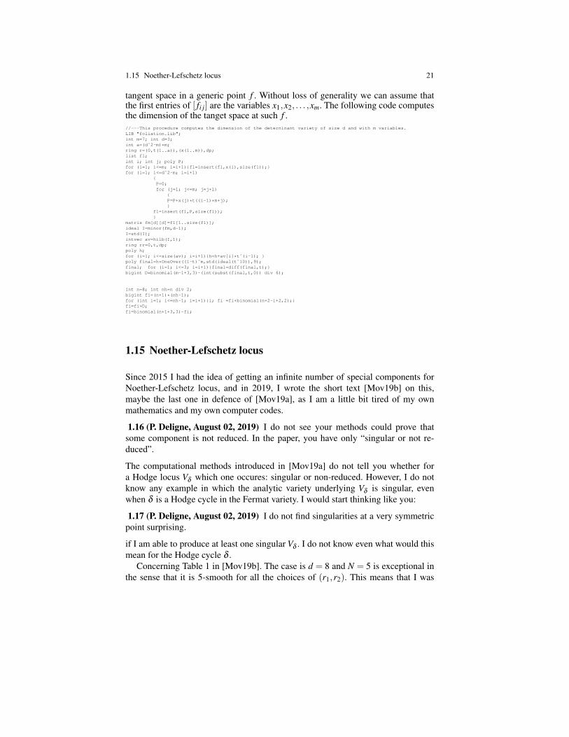
1.15 Noether-Lefschetz locus 21

tangent space in a generic point f . Without loss of generality we can assume thatthe first entries of [ fi j] are the variables x1,x2, . . . ,xm. The following code computesthe dimension of the tanget space at such f .//---This procedure computes the dimension of the deterninant variety of size d and with m variables.LIB "foliation.lib";int m=7; int d=3;int a=(dˆ2-m)*m;ring r=(0,t(1..a)),(x(1..m)),dp;list fl;int i; int j; poly P;for (i=1; i<=m; i=i+1)fl=insert(fl,x(i),size(fl));for (i=1; i<=dˆ2-m; i=i+1)

P=0;for (j=1; j<=m; j=j+1)

P=P+x(j)*t((i-1)*m+j);

fl=insert(fl,P,size(fl));

matrix fm[d][d]=fl[1..size(fl)];ideal I=minor(fm,d-1);I=std(I);intvec av=hilb(I,1);ring rr=0,t,dp;poly h;for (i=1; i<=size(av); i=i+1)h=h+av[i]*tˆ(i-1); poly final=h*OneOver((1-t)ˆm,std(ideal(tˆ10)),9);final; for (i=1; i<=3; i=i+1)final=diff(final,t);bigint D=binomial(m-1+3,3)-(int(subst(final,t,0)) div 6);

int n=8; int nh=n div 2;bigint fi=(n+1)*(nh-1);for (int i=1; i<=nh-1; i=i+1)i; fi =fi+binomial(n+2-i+2,2);fi=fi+D;fi=binomial(n+1+3,3)-fi;

1.15 Noether-Lefschetz locus

Since 2015 I had the idea of getting an infinite number of special components forNoether-Lefschetz locus, and in 2019, I wrote the short text [Mov19b] on this,maybe the last one in defence of [Mov19a], as I am a little bit tired of my ownmathematics and my own computer codes.

1.16 (P. Deligne, August 02, 2019) I do not see your methods could prove thatsome component is not reduced. In the paper, you have only “singular or not re-duced”.

The computational methods introduced in [Mov19a] do not tell you whether fora Hodge locus Vδ which one occures: singular or non-reduced. However, I do notknow any example in which the analytic variety underlying Vδ is singular, evenwhen δ is a Hodge cycle in the Fermat variety. I would start thinking like you:

1.17 (P. Deligne, August 02, 2019) I do not find singularities at a very symmetricpoint surprising.

if I am able to produce at least one singular Vδ . I do not know even what would thismean for the Hodge cycle δ .

Concerning Table 1 in [Mov19b]. The case is d = 8 and N = 5 is exceptional inthe sense that it is 5-smooth for all the choices of (r1,r2). This means that I was


supposed to analyse 6-smoothness, however, this was beyond the capacity of mycomputer (5-smoothness already took more than 10 days of computations).

1.18 (P. Deligne, August 02, 2019) The factors you take [in the definition of thecurve C2] are “consecutive”. Does this matter?

Personally, I think this does not matter, even though one cannot get this fact us-ing the automorphism of the Fermat variety or using Galois symmetry, as you havementioned in your letter. I can start writting codes for other combinations of rootsused in the curves C1 and C2 and observe that a similar phenomena happens. As-suming the main conjecture (discovery) of [Mov19b], that is, V[C1]+rC2 , r ∈Q are 31codimensional smooth varieties, one can argue that such consecutive roots do notmatter. This is as follows. Let S⊂ Tfull be the parametrs space of surfaces containga line C1 and a complete intersection curve C2 of type (3,3) with C1∩C2 = /0. SinceV[C1]∩V[C2] is of codimension 32, it is just a branch of S. It might not be so hard toprove that S is irreducible. If this is the case then all other possible arrangement ofthe roots of unity for defining C1 and C2 will produce different branches of S.

1.16 A fundamental proposition of [Mov20a]

(9 August 2019) How you would feel if you built up a mathematical theory basedon a proposition, and after the theory is around 250 pages, you realize that you havenot a rigorous proof for such a proposition? You may feel that the whole theorymight be an abstract nonsense , however, you go through the theory and you seethat even though the proof of the fundamental proposition lacks rigor, somethingbeautiful is going on, and you are not allowed to judge the whole theory based onthis. Nowadays, I have such feelings and I am trying to find a rigorous proof for thefollowing statement. This is Proposition 2.4 of [Mov20a].

Proposition 1.11 Let Xt , t ∈ T be a family of smooth projective varieties and letX ,X0 be two regular fibers of this family. We have an isomorphism

(H∗dR(X),F∗,∪,θ) α' (H∗dR(X0),F∗0 ,∪,θ0) (1.30)

For the proof I had written the following: It is enough to prove the isomorphism(1.30) for X = Xt with t in a Zariski neighborhood of 0 ∈ T. We can take sectionsαm,i of the cohomology bundle Hm

dR(X/T) in a Zariski open neighborhood U of0 such that θ i’s are included in this basis, and moreover, it is compatible with theHodge filtration and cup product for all t ∈U . This basis will produce the requiredisomorphism (1.30) for X0 and X .

I woke up from my dream of seeing the fruitful corners of [Mov20a] after thefollowing:

1.19 (P. Deligne, May 12, 2019) I think you are overoptimistic in 2.4 page 14 [theabove proposition]: while it might be true in examples you consider, I don’t expect

1.16 A fundamental proposition of [Mov20a] 23

you can in general find sections compatible both with the cup-product and the Hodgefiltration.

After few hours, I got the following:

1.20 (P. Deligne, May 12, 2019) On second thought, 2.14 is correct (but the proofis not convincing). It suffices to consider families over C. Let G be the (linear alge-braic) group of automorphisms of (H, cup product, polarization). The Hodge decom-position is given by the action of Gm: multiplication by zp−q on H p,q. This action isa morphism to G. One then uses that nearby morphisms from Gm to G are conjugate.

As an ignorant person in the theory of algebraic groups developed by A. Borel andmany other respected mathematicians, I had to dig up the literature in order to un-derstand why the last sentence “One then uses that nearby morphisms from Gm to Gare conjugate” is true. I only found the following: Let G be a linear algebraic groupover a field k (for safeness, characteristic zero and algebraically closed). All max-imal tori T in G are G(k)-conjugate, see for instance [Con14, Proposition 1.1.19,2]. The maximality cannot be dropped from this statement. However, the situationin Proposition 1.11 is slightly different: we have families of Gm → G, that is, wehave a morphism Gm×T→ G of algebraic varieties such that for fixed t ∈ T, themap Gm×t→ G is a morphism of algebraic groups. So far, I am able to producesuch families by conjugation of a fixed morphism Gm → G, and it is clear from P.Deligne’s comments, there is a theorem which says that this is always the case. Aftera day or so, I failed to find a reference or prove by myself the following:

1.1 Is the following true? Let Gm be the multiplicative group (C−0, ·), G alinear algebraic group and T be an irreducible affine variety, all over C. Let alsof : Gm×T→ G be a family of algebraic group morphisms, that is, for fixed t ∈ T,the map Gm×t → G is a morphism of algebraic groups. Then there is a map g :T→G and algebraic group morphism i : Gm→G such that f (g, t)= g(t)i(g)g(t)−1.

I wrote back to P. Deligne: I tried to find a reference or prove by myself the ”Onethen uses that nearby morphisms from Gm to G are conjugate” part of your email. Idid not succeed and it seems that my brain is spoiled with too much heavy computercalculations!

1.21 (P. Deligne, August 14, 2019) My reference is SGA 3. IX 3 uses cohomologyto obtain infinitesimal statements. XI 4 proves representability of the functor M ofsubgroupschemes of multiplicative type. XI 5 puts it all together to prove that for anaffine smooth groupscheme G/S, and M the scheme parametrizing subgroupschemeof multiplicative type, M is smooth over S and the action by conjugation of G on Mgives a smooth morphism (action, IdM) : GxM−> MxM.

Chapter 2Some experiments with SmoothReduced offoliation.lib

We describe how to use the library foliation.lib of Singular in order tostudy the components of the Hodge loci passing through the Fermat point.

2.1 Introduction

This article is supposed to contain many computational details which are missing inthe article [Mov17c]. For all definitions see this article.

2.2 Sum of two linear cycles

I have used the following code for Theorem 2 and Theorem 3 of [Mov17c]. We canchange the dimension n, the degree d and the degree of truncation tru.LIB "foliation.lib";int n=2; int d=10; int m=n div 2-1; int tru=2; int zb=10;intvec zarib1=1,-zb; intvec zarib2=zb,zb;intvec mlist=d; for (int i=1;i<=n; i=i+1)mlist=mlist,d;ring r=(0,z), (x(1..n+1)),dp;poly cp=cyclotomic(2*d); int degext=deg(cp) div deg(var(1));cp=subst(cp, x(1),z); minpoly =number(cp);list lcycles=SumTwoLinearCycle(n,d,m,1); lcycles;list ll=SmoothReduced(mlist,tru, lcycles, zarib1, zarib2);ll[1];string sss="(n,d,m,tru)=("+string(n)+","+string(d)+","+string(m)+","+string(tru)+")"+"--Smooth and Reduced";write(":a ReducedSmoothOutputFinal", sss);sss="Number of reduced cases=", string(size(ll[1]));write(":a ReducedSmoothOutputFinal", sss);write(":a ReducedSmoothOutputFinal", ll[1]);sss="Number of noreduced cases=", string(size(ll[2]));write(":a ReducedSmoothOutputFinal", sss);write(":a ReducedSmoothOutputFinal", ll[2]);write(":a ReducedSmoothOutputFinal", "**********************************************************");

In the following we are goint to take Pn2i , ri ∈ Z, i = 1,2, · · · ,s and consider the

cycle

δ :=s

∑i=1

ri[Pn2i ] ∈ Hn(Xd

n ,Z). (2.1)

25

26 2 Some experiments with SmoothReduced of foliation.lib

and the corresponding Hodge locus Vδ . We will assume that

r1 ≥ 1, |ri| ≤ zb := 10, ri 6= 0.

Therefore, in total we have 21s−1 ·10 cycles. In the codes below, zb = 10. In somecases, I had to take smaller zb in order to either make the computations faster orunderstand the structure of reduced and non-reduced cases.

2.3 Noether-Lefschetz locus: three lines crossing a point

We investigate the Hodge loci corresponding to three lines crossing a point in theFermat surface.LIB "foliation.lib";int n=2; int d=5; int tru=3; int zb=10;intvec zarib1=1,-zb,-zb; intvec zarib2=zb,zb,zb;intvec mlist=d; for (int i=1;i<=n; i=i+1)mlist=mlist,d;ring r=(0,z), (x(1..n+1)),dp;poly cp=cyclotomic(2*d); int degext=deg(cp) div deg(var(1));cp=subst(cp, x(1),z); minpoly =number(cp);list lcycles=list(intvec(0,0,0,0),intvec(0,1,2,3)),

list(intvec(0,0,0,1),intvec(0,1,2,3)),list(intvec(0,0,0,2),intvec(0,1,2,3));

list ll=SmoothReduced(mlist,tru, lcycles, zarib1, zarib2);

1. For d = 5 the Hodge locus Vδ is 2-reduced. It is 3-reduced only in the expectedcases:

(r1 = r2 = r3) or (r2 = 0&r1 = r3) or (r3 = 0,r1 = r2), or (r2 = r3 = 0). (2.2)

Note that the first Hodge locus is actually reduced because the correspondingcurve can be deformed into a curve which is a complete intersection of type 1,3.

2. For d = 6 the Hodge locus Vδ is NOT 2-reduced only if one of ri is zero and theother two are non-zero and not equal to each other. It is 3-reduced only in theexpected cases (2.2). The computation took few hours.

3. For d = 7 the Hodge locus Vδ is 2-reduced only in the expcted cases (2.2).

2.4 Noether-Lefschetz locus: three lines forming U

We consider three lines P1i , i = 1,2,3 such tha P1

1 ·P12 = P1

1 ·P13 = 1 and all other

intersections are zero.LIB "foliation.lib";int n=2; int d=6; int tru=2; int zb=10;intvec zarib1=1,-zb,-zb; intvec zarib2=zb,zb,zb;intvec mlist=d; for (int i=1;i<=n; i=i+1)mlist=mlist,d;ring r=(0,z), (x(1..n+1)),dp;poly cp=cyclotomic(2*d); int degext=deg(cp) div deg(var(1));cp=subst(cp, x(1),z); minpoly =number(cp);list lcycles=ListPeriodLinearCycle(n,d,1);list lcycles=list(intvec(0,0,0,0),intvec(0,1,2,3)),

list(intvec(0,0,0,1),intvec(0,1,2,3)),list(intvec(0,1,0,0),intvec(0,1,2,3));

list ll=SmoothReduced(mlist,tru, lcycles, zarib1, zarib2);

2.6 Noether-Lefschetz loci: The most simple tree 27

Note that in the code above the first line intersects the second and third line.

1. For d = 5, all the hodge locus Vδ is 2-reduced. It is NOT 3- and 4-reduced in thecases

(r2 = 0&r1 6= r3) or (r3 = 0&r1 6= r2) (2.3)

which is 10 ∗ 19+ 10 ∗ 19 cases. It seems that in this cases there are infininitenumber of components of the Hodge loci crossing the Fermat point.

2. For d = 6,7, Vδ is 2-reduced only in the cases:

(r1 = r2 = r3) or (r2 = 0, r1 = r3) or (r3 = 0, r1 = r2) or (r2 = r3 = 0) (2.4)

which is 10+ 10+ 10+ 10 cases. In the first case, it seems to me that the threelines can be deformed into an irreducible curve of degree 3 in a surface.

2.5 Noether-Lefschetz locus: all the lines together

In this section we take the linear combination of all the lines in the Fermat surface.It is too much. It takes an eternity!!!!LIB "foliation.lib";int n=2; int d=5; int tru=2; int zb=10;

//-Producing the list of all lines-----intvec zv=0,0; intvec dm1=0,d-1; for(int i=2;i<=n div 2+1; i=i+1)

zv=zv,0,0; dm1=dm1, 0,d-1;list a=aIndex(zv,dm1); list b=bIndex(n+2); int j;for(i=1;i<=size(b); i=i+1) for(j=1;j<=n+2; j=j+1) b[i][j]=b[i][j]-1;list lcycles;for(j=1;j<=size(a); j=j+1)

for(i=1;i<=size(b); i=i+1)lcycles=insert(lcycles, list(a[j],b[i]), size(lcycles));

//-------------------------------------

int N=size(lcycles);intvec zarib1=1; intvec zarib2=zb; for(i=2;i<=N; i=i+1)zarib1=zarib1,-zb; zarib2=zarib2,zb;intvec mlist=d; for (int i=1;i<=n; i=i+1)mlist=mlist,d;ring r=(0,z), (x(1..n+1)),dp;poly cp=cyclotomic(2*d); int degext=deg(cp) div deg(var(1));cp=subst(cp, x(1),z); minpoly =number(cp);list ll=SmoothReduced(mlist,tru, lcycles, zarib1, zarib2);

2.6 Noether-Lefschetz loci: The most simple tree

After the computations in §2.4 for d = 5, it seemed reasonable to analyze the mostsimple three of lines, that is, P1

i , i = 1,2, . . . ,M with P1i ·P1

i+1 = 1, i = 1,2, . . . ,M−1, and no other intersectin point. Note that for M = 3 the order of lines is differentas in (2.4). In the code below I produce one such a tree among d2 group of linescorresponding to 3d2 = d2 +d2 +d2. For instance for M = 5 it produces the lines:[1]:

[1]:0,0,0,0

[2]:0,1,2,3

[2]:[1]:

0,0,0,1


Fig. 2.1 A simple Tree of linear cycles

[2]:0,1,2,3

[3]:[1]:

0,1,0,1[2]:

0,1,2,3[4]:

[1]:0,1,0,2

[2]:0,1,2,3

[5]:[1]:

0,2,0,2[2]:

0,1,2,3

It could be also useful to take a tree jumping from one group of d2 lines to anothergroup. In the code below the number M of lines must be at most 2d +1, see Figure2.1.LIB "foliation.lib";int n=2; int d=6; int tru=3; int zb=4;int M=5; //---the size of the treeintvec a=intvec(0,0,0,0); intvec b=intvec(0,1,2,3); list lcycles=list(list(a,b)); int k; int i;intvec zarib1=1; intvec zarib2=zb;for (i=1;i<=M-1; i=i+1)

k=i div 2; if (2*k==i) a=intvec(0,k,0,k);else a=intvec(0,k,0,k+1);lcycles=insert(lcycles, list(a,b), size(lcycles));zarib1=zarib1,-zb; zarib2=zarib2,zb;

lcycles;intvec mlist=d; for (int i=1;i<=n; i=i+1)mlist=mlist,d;ring r=(0,z), (x(1..n+1)),dp;poly cp=cyclotomic(2*d); int degext=deg(cp) div deg(var(1));cp=subst(cp, x(1),z); minpoly =number(cp);list ll=SmoothReduced(mlist,tru, lcycles, zarib1, zarib2);

In the following the number of lines is 4, that is, M = 4.

1. For d = 5, the Hodge locus Vδ is always 2-reduced. It is NOT 3-reduced only inthe cases:

(r3 = r4 = 0, r1 6= r2, r2 6= 0)

2.7 Some heavy computation made in December 2017 29

which is 10 ∗ 21− 10− 10 = 190 cases. To be sure, I also checked that Vδ isNOT 4-reduced only in the above cases. THIS IS NOT STRANGE. Note thatthe first coefficients is never zero, and so, the result says that as soon as we addnon-zero multiple of a one or two lines which does not intersect the first one,then the Hodge loci becomes 3-reduced. Therefore, this is not in contradictionwith Voisin’s result that the loci of sum of two lines in a surface is reduced if andonly if either one of the coefficients is zero or two coefficients are equal. In thiscase it seems that we have an infinite number of components of the Hodge locucrossing Fermat.

2. The case d = 6, I started to analyze 2-reducedness. I was not able to find a sim-ple logical statement distinguishing the set of reduced cases from non-reducedcases. In what follows the text is hyperlinked to the corresponding data in myhomepage. For zb= 2 we have in total 2∗53 = 250 cases from which only 118cases are 2-reduced. For zb= 4 we have 844 reduced cases and for zb= 10 wehave 12430 reduced cases. This pattern seemed to me strange, and in fact it is dif-ferent from, the pattern for d = 7,8 below. I checked the 3-reducedness and getthe same pattern as for higher degrees. For zb= 4 there are only 144 3-reducedcases.

3. This strange pattern from d = 7,8, · · · changes. For zb= 4 and d = 7, 144 casesare reduced. For zb = 4 and d = 8, 144 cases are reduced. Therefore, it seemsthat for d ≥ 7 the structure of 2-reducedness is the same.

Analysing the cases d = 7,8 I started to think on Conjecture 4.1.

2.7 Some heavy computation made in December 2017

In this section I report on more computations for sum of linear cycles as in §2.6.

1. n = 2, d = 5, tru = 4, zb = 4, M = 5. The data of this computation can be foundhere. The Hodge locus in NOT reduced only when

r3 = r4 = r5 = 0,r2 6= 0,r2 6= r1.

which are 28 cases. It seems that in this cases there are infininite number ofcomponents of the Hodge loci crossing the Fermat point.

2. n = 2, d = 7, tru = 2, zb = 4, M = 5. There are 2864 2-reduced cases!. Noidea what to say. Most of the cases the tree is disconnected, that is, one of thecofficients ri is zero.

3. n = 2, d = 6, tru = 3, zb = 4, M = 5. The same comment as above! There are5264 which are NOT 3-reduced cases!. NO idea what to say. Have a look at thedata by yourself.

4. n = 2, d = 6, tru = 2, zb = 4, M = 6.5. n = 2, d = 8, tru = 2, zb = 4, M = 5. FEW DAYS Of Computing. More than

55GB of Swap+16Mem is used.

http://w3.impa.br/~hossein/WikiHossein/files/Data/2017_12_d=6_n=2_4Cycles_2ReducedCases_zb=2.txt










http://w3.impa.br/~hossein/WikiHossein/files/Singular%20Codes/2017-12_n=2_d=5_tru=4_M=5.txt



http://w3.impa.br/~hossein/WikiHossein/files/Singular%20Codes/2017-12-n=2_d=6_tru=3_M=5.txt





6. n = 2, d = 7, tru = 3, zb = 4, M = 5. 15 days of computing.7. n = 2, d = 7, tru = 3, zb = 4, M = 5. 30 days of computing. 101GB swap+16GB

memory used.

2.8 Noether-Lefschetz loci: four lines forming a square

Here we take four lines forming a square.LIB "foliation.lib";int n=2; int d=7; int tru=2; int zb=4;intvec zarib1=1,-zb,-zb,-zb; intvec zarib2=zb,zb,zb,zb;intvec mlist=d; for (int i=1;i<=n; i=i+1)mlist=mlist,d;ring r=(0,z), (x(1..n+1)),dp;poly cp=cyclotomic(2*d); int degext=deg(cp) div deg(var(1));cp=subst(cp, x(1),z); minpoly =number(cp);list lcycles=list(intvec(0,0,0,0),intvec(0,1,2,3)),

list(intvec(0,0,0,1),intvec(0,1,2,3)),list(intvec(0,1,0,1),intvec(0,1,2,3)),list(intvec(0,1,0,0),intvec(0,1,2,3));

lcycles; zarib1;zarib2;list ll=SmoothReduced(mlist,tru, lcycles, zarib1, zarib2);

1. For d = 5 and zb= 4 we have only 56= 28+28 cases in which Vδ is NOT 3- and4-reduced. These are exactly those with the coefficients zero, the correspondinglines intersect each other, and the other coefficints are non-zero and non-equal.

(a,b,0,0),(a,0,0,b),a,b, 6= 0, a 6= b.

2. For d = 6,7,8 and zb= 4 we have only 60 = 36+4+4+4+4+4+4 2-reducedcases.

(a,0,b,0),

(a,a,0,0),(a,0,0,a),(a,a,0,a),(a,a,a,0),(a,0,a,a),(a,a,a,a)

The novelty here is that (1,1,1,1) is included in the 2-reduced cases.

2.9 Noether-Lefschetz loci: E shape arrangement

http://w3.impa.br/~hossein/WikiHossein/files/Singular%20Codes/2017-12-n=2_d=7_tru=3-M=5-15days.txt

http://w3.impa.br/~hossein/WikiHossein/files/Singular%20Codes/2017-12-n=2_d=7_M=5_30days_101+16GB.txt

Chapter 3Computing a PF system

These are the notes of my math conversations with P. Berglund in January 2019.

3.1 Set-up

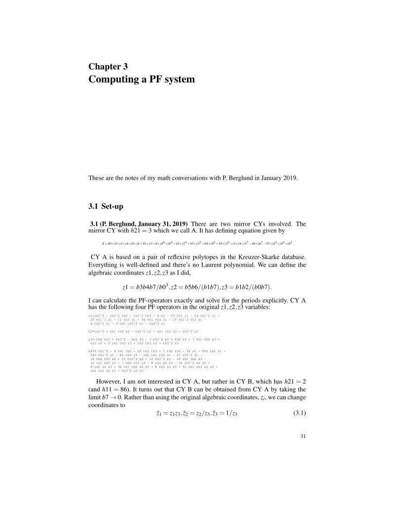
3.1 (P. Berglund, January 31, 2019) There are two mirror CYs involved. Themirror CY with h21 = 3 which we call A. It has defining equation given by

A = b0∗ y2∗ y3∗ y4∗ y5∗ y6+b1∗ y3∗ y4∗ y54 ∗ y64 +b2∗ y24 +b3∗ y33 +b4∗ y43 +b5∗ y23 ∗ y3∗ y4∗ y57 −b6∗ y67 −b7∗ y23 ∗ y53 ∗ y63

CY A is based on a pair of reflexive polytopes in the Kreuzer-Skarke database.Everything is well-defined and there’s no Laurent polynomial. We can define thealgebraic coordinates z1,z2,z3 as I did,

z1 = b3b4b7/b03,z2 = b5b6/(b1b7),z3 = b1b2/(b0b7).

I can calculate the PF-operators exactly and solve for the periods explicitly. CY Ahas the following four PF operators in the original z1,z2,z3 variables:L1=th1ˆ3 - th1ˆ2 th2 - th1ˆ2 th3 - 6 z1 - 33 th1 z1 - 54 th1ˆ2 z1 -27 th1ˆ3 z1 - 11 th3 z1 - 36 th1 th3 z1 - 27 th1ˆ2 th3 z1 -6 th3ˆ2 z1 - 9 th1 th3ˆ2 z1 - th3ˆ3 z1

L2=th2ˆ2 + th1 th2 z2 - th2ˆ2 z2 - th1 th3 z2 + th3ˆ2 z2

L3=-th2 th3 + th3ˆ2 - th1 z3 - 3 th1ˆ2 z3 + th2 z3 + 3 th1 th2 z3 +th3 z3 + 2 th1 th3 z3 + th2 th3 z3 + th3ˆ2 z3

L4=9 th1ˆ2 - 9 th1 th2 - 12 th1 th3 + 7 th2 th3 - 54 z1 - 243 th1 z1 -243 th1ˆ2 z1 - 81 th3 z1 - 162 th1 th3 z1 - 27 th3ˆ2 z1 -15 th2 th3 z2 + 15 th3ˆ2 z2 + 12 th1ˆ2 z3 - 19 th1 th2 z3 -12 th1 th3 z3 + 7 th2 th3 z3 - 8 th1 z2 z3 - 52 th1ˆ2 z2 z3 +8 th2 z2 z3 + 52 th1 th2 z2 z3 + 8 th3 z2 z3 + 51 th1 th3 z2 z3 +th2 th3 z2 z3 + th3ˆ2 z2 z3

However, I am not interested in CY A, but rather in CY B, which has h21 = 2(and h11 = 86). It turns out that CY B can be obtained from CY A by taking thelimit b7→ 0. Rather than using the original algebraic coordinates, zi, we can changecoordinates to

z1 = z1z3, z2 = z2/z3, z3 = 1/z3 (3.1)

31

32 3 Computing a PF system

in which case b7→ 0 is obtained by taking z3→ 0. Note that both z1andz2 are finitein this limit which is how we remain with the two complex structure deformationsfor CY B. The problem is that I do not know how to find the PF operators for the CYB model from the PF operators for CY A. I do know the defining equation whichtakes the form-note the Laurent monomial:

B = c0∗w2∗w3∗w4∗w5∗w6+ c1∗w54 ∗w64 + c2∗w24 + c3∗w34 + c4∗w44 + c5∗w23 ∗w3( −1)∗w4( −1)∗w57 − c6∗w67

We can define new algebraic coordinates in terms of the above ci,

z1 = c1c2c3c4/c04, z2 = c0c5c6/c13.

Since the b7→ 0 limit of CY A is supposed to give CY B, I believe that zi = zi. Infact, I can check this by taking suitable linear combinations of the periods for CY Aand then making the change of variables in the 7

¯→ 0 limit, to obtain periods which

I can compare with from what I can obtain directly for CY B. However, I do notknow how obtain the complete set of PF operators for CY B.

By chain rule for (3.1) we have:

θ1 = θ1

θ2 = θ2

θ3 = θ1− θ2− θ3

Note that θzn = zn(θ +n).

3.2 Restricting non-commutative rings

In this section I will use some techniques used in [HMY17]. In particulary, I amgoing to use the procedure restrictionIdeal of dmosapp.lib written byViktor Levandovskyy and Daniel Andres.//|||||2019-Per-Berglund three parameter family of K3 fibered CY3|intvec w = 0,0,1; // 1 at the place of z_3, the rest are 0. This is the limit z3=0-----------LIB "nctools.lib";ring r = 0, (z1,z2,z3,t1,t2,t3),dp;def R = Weyl(); setring R;poly th1=z1*t1; poly th2=z2*t2; poly th3=z3*t3;

poly L1 = th1ˆ2*th3 - 6*z1*z3 - 44*z1*z3*th1 - 96*z1*z3*th1ˆ2 -64*z1*z3*th1ˆ3 + 11*z1*z3*th2 + 48*z1*z3*th1*th2 +48*z1*z3*th1ˆ2*th2 - 6*z1*z3*th2ˆ2 - 12*z1*z3*th1*th2ˆ2 +z1*z3*th2ˆ3 + 11*z1*z3*th3 + 48*z1*z3*th1*th3 + 48*z1*z3*th1ˆ2*th3 -12*z1*z3*th2*th3 - 24*z1*z3*th1*th2*th3 + 3*z1*z3*th2ˆ2*th3 -6*z1*z3*th3ˆ2 - 12*z1*z3*th1*th3ˆ2 + 3*z1*z3*th2*th3ˆ2 + z1*z3*th3ˆ3;

poly L2 = -z2*th1*th3 + 2*z2*th2*th3 + z2*th3ˆ2 + z3*th2ˆ2;

poly L3 = -th3 - 4*th1*th3 + th2*th3 + th3ˆ2 + z3*th1ˆ2 - 3*z3*th1*th2 +2*z3*th2ˆ2 - 2*z3*th1*th3 + 3*z3*th2*th3 + z3*th3ˆ2;

poly L4 = -8*z2*th3 - 53*z2*th1*th3 + z2*th2*th3 + z2*th3ˆ2 - 7*z3*th2ˆ2 +12*z3*th1*th3 - 7*z3*th2*th3 + 15*z2*z3*th1ˆ2 - 45*z2*z3*th1*th2 +30*z2*z3*th2ˆ2 - 30*z2*z3*th1*th3 + 45*z2*z3*th2*th3 +15*z2*z3*th3ˆ2 - 3*z3ˆ2*th1ˆ2 + 10*z3ˆ2*th1*th2 - 7*z3ˆ2*th2ˆ2 +12*z3ˆ2*th1*th3 - 7*z3ˆ2*th2*th3 - 54*z1*z3ˆ3 - 324*z1*z3ˆ3*th1 -432*z1*z3ˆ3*th1ˆ2 + 81*z1*z3ˆ3*th2 + 216*z1*z3ˆ3*th1*th2 -27*z1*z3ˆ3*th2ˆ2 + 81*z1*z3ˆ3*th3 + 216*z1*z3ˆ3*th1*th3 -54*z1*z3ˆ3*th2*th3 - 27*z1*z3ˆ3*th3ˆ2;

3.3 Picard-Fuchs ideal 33

//--new code suggested by V. Levandovskyy February 04, 2019.ideal I=L1, L2,L3, L4;I = slimgb(I); // computes a left Groebner basisdim(I); // Gelfand-Kirillov dimension; 3 in this caseLIB "dmodapp.lib";def Rz2 = restrictionIdeal(I,w);setring Rz2;ideal II=resIdeal;

ideal III=slimgb(II);

//--Old code suggested by V. Levandovskyy.//-ideal I=L1, L2,L3, L4;//-I = std(I); // computes a left Groebner basis//-dim(I);//-LIB "dmodapp.lib";//-def Rz2 = restrictionModule(I,w);//-setring Rz2;//-print(resMod); // the ideal J you ask for// We divide the result by gen(1) and z1.//-module II=resMod;//-ideal I; for (int i=1; i<=11; i=i+1) I=I, II[1,i];

Answer:resIdeal[1]=z1ˆ3*z2*t1ˆ3-5*z1ˆ2*z2ˆ2*t1ˆ2*t2+8*z1*z2ˆ3*t1*t2ˆ2-4*z2ˆ4*t2ˆ3-4*z1*z2ˆ2*t1*t2ˆ2+z2ˆ3*t2ˆ3+2*z1ˆ2*z2*t1ˆ2+6*z1*z2ˆ2*t1*t2-14*z2ˆ3*t2ˆ2-4*z1*z2*t1*t2+2*z2ˆ2*t2ˆ2-6*z2ˆ2*t2resIdeal[2]=840*z1ˆ3*z2ˆ2*t1ˆ2*t2-2331*z1ˆ2*z2ˆ3*t1*t2ˆ2+1302*z1*z2ˆ4*t2ˆ3-1024*z1ˆ4*t1ˆ3+768*z1ˆ3*z2*t1ˆ2*t2+1152*z1ˆ2*z2ˆ2*t1*t2ˆ2-320*z1*z2ˆ3*t2ˆ3+588*z1ˆ3*z2*t1ˆ2+4*z1ˆ3*t1ˆ3-3066*z1ˆ2*z2ˆ2*t1*t2-11*z1ˆ2*z2*t1ˆ2*t2+4704*z1*z2ˆ3*t2ˆ2-4608*z1ˆ3*t1ˆ2+2688*z1ˆ2*z2*t1*t2-720*z1*z2ˆ2*t2ˆ2+630*z1ˆ2*z2*t1+12*z1ˆ2*t1ˆ2+2016*z1*z2ˆ2*t2-11*z1*z2*t1*t2-3264*z1ˆ2*t1+96*z1*z2*t2+4*z1*t1-96*z1resIdeal[3]=1869*z1ˆ2*z2ˆ3*t1ˆ2*t2ˆ2-5418*z1*z2ˆ4*t1*t2ˆ3+3360*z2ˆ5*t2ˆ4-1024*z1ˆ4*t1ˆ4+4992*z1ˆ2*z2ˆ2*t1ˆ2*t2ˆ2-3104*z1*z2ˆ3*t1*t2ˆ3+2232*z2ˆ4*t2ˆ4+4*z1ˆ3*t1ˆ4+4914*z1ˆ2*z2ˆ2*t1ˆ2*t2-11*z1ˆ2*z2*t1ˆ3*t2-23142*z1*z2ˆ3*t1*t2ˆ2+25494*z2ˆ4*t2ˆ3+3072*z1*z2ˆ2*t1*t2ˆ3-768*z2ˆ3*t2ˆ4-9472*z1ˆ3*t1ˆ3+11136*z1ˆ2*z2*t1ˆ2*t2-12384*z1*z2ˆ2*t1*t2ˆ2+18772*z2ˆ3*t2ˆ3+1218*z1ˆ2*z2*t1ˆ2+24*z1ˆ2*t1ˆ3-12684*z1*z2ˆ2*t1*t2-33*z1*z2*t1ˆ2*t2+41496*z2ˆ3*t2ˆ2+9216*z1*z2*t1*t2ˆ2-3840*z2ˆ2*t2ˆ3-18624*z1ˆ2*t1ˆ2-1392*z1*z2*t1*t2+33288*z2ˆ2*t2ˆ2+1260*z1*z2*t1+28*z1*t1ˆ2+10584*z2ˆ2*t2+3072*z1*t1*t2-11*z2*t1*t2-3072*z2*t2ˆ2-6624*z1*t1+9312*z2*t2+4*t1-96resIdeal[4]=26880*z1ˆ5*t1ˆ4-131628*z1ˆ2*z2ˆ3*t1*t2ˆ3+85281*z1*z2ˆ4*t2ˆ4-105*z1ˆ4*t1ˆ4-151552*z1ˆ4*t1ˆ3*t2+113664*z1ˆ3*z2*t1ˆ2*t2ˆ2+1365*z1ˆ2*z2ˆ2*t1ˆ2*t2ˆ2+62976*z1ˆ2*z2ˆ2*t1*t2ˆ3-2520*z1*z2ˆ3*t1*t2ˆ3-20480*z1*z2ˆ3*t2ˆ4+1260*z2ˆ4*t2ˆ4+255360*z1ˆ4*t1ˆ3-336*z1ˆ3*z2*t1ˆ2*t2+592*z1ˆ3*t1ˆ3*t2-664692*z1ˆ2*z2ˆ2*t1*t2ˆ2-1628*z1ˆ2*z2*t1ˆ2*t2ˆ2+660156*z1*z2ˆ3*t2ˆ3+1260*z1*z2ˆ2*t1*t2ˆ3-315*z2ˆ3*t2ˆ4-945*z1ˆ3*t1ˆ3-568320*z1ˆ3*t1ˆ2*t2+3255*z1ˆ2*z2*t1ˆ2*t2+416256*z1ˆ2*z2*t1*t2ˆ2-9660*z1*z2ˆ2*t1*t2ˆ2-114240*z1*z2ˆ2*t2ˆ3+9450*z2ˆ3*t2ˆ3+589344*z1ˆ3*t1ˆ2-577416*z1ˆ2*z2*t1*t2+148*z1ˆ2*t1ˆ2*t2+1097964*z1*z2ˆ2*t2ˆ2+2152*z1*z2*t1*t2ˆ2-1575*z2ˆ2*t2ˆ3-1365*z1ˆ2*t1ˆ2-192768*z1ˆ2*t1*t2-3675*z1*z2*t1*t2-91392*z1*z2*t2ˆ2+15120*z2ˆ2*t2ˆ2+267120*z1ˆ2*t1+271656*z1*z2*t2+224*z1*t1*t2-1260*z2*t2ˆ2-105*z1*t1+3780*z2*t2+2520*z1resIdeal[5]=428064*z1ˆ2*z2ˆ3*t1*t2ˆ4-279888*z1*z2ˆ4*t2ˆ5+557056*z1ˆ4*t1ˆ3*t2ˆ2-561834*z1ˆ2*z2ˆ3*t1*t2ˆ3-417792*z1ˆ3*z2*t1ˆ2*t2ˆ3-960*z1ˆ2*z2ˆ2*t1ˆ2*t2ˆ3+367353*z1*z2ˆ4*t2ˆ4-196608*z1ˆ2*z2ˆ2*t1*t2ˆ4+2880*z1*z2ˆ3*t1*t2ˆ4+66560*z1*z2ˆ3*t2ˆ5-1920*z2ˆ4*t2ˆ5-669696*z1ˆ4*t1ˆ3*t2+451200*z1ˆ3*z2*t1ˆ2*t2ˆ2+1260*z1ˆ2*z2ˆ2*t1ˆ2*t2ˆ2-2176*z1ˆ3*t1ˆ3*t2ˆ2+3719616*z1ˆ2*z2ˆ2*t1*t2ˆ3-3780*z1*z2ˆ3*t1*t2ˆ3+5984*z1ˆ2*z2*t1ˆ2*t2ˆ3-3376080*z1*z2ˆ3*t2ˆ4+2520*z2ˆ4*t2ˆ4-1680*z1*z2ˆ2*t1*t2ˆ4+480*z2ˆ3*t2ˆ5+80640*z1ˆ4*t1ˆ3-28728*z1ˆ3*z2*t1ˆ2*t2+2616*z1ˆ3*t1ˆ3*t2-2809926*z1ˆ2*z2ˆ2*t1*t2ˆ2+1671168*z1ˆ3*t1ˆ2*t2ˆ2-11454*z1ˆ2*z2*t1ˆ2*t2ˆ2+2842308*z1*z2ˆ3*t2ˆ3-1818624*z1ˆ2*z2*t1*t2ˆ3+22365*z1*z2ˆ2*t1*t2ˆ3+576000*z1*z2ˆ2*t2ˆ4-22710*z2ˆ3*t2ˆ4-315*z1ˆ3*t1ˆ3-2613504*z1ˆ3*t1ˆ2*t2+4095*z1ˆ2*z2*t1ˆ2*t2+7908288*z1ˆ2*z2*t1*t2ˆ2-16380*z1*z2ˆ2*t1*t2ˆ2+5440*z1ˆ2*t1ˆ2*t2ˆ2-10606176*z1*z2ˆ2*t2ˆ3+18900*z2ˆ3*t2ˆ3-2416*z1*z2*t1*t2ˆ3+3840*z2ˆ2*t2ˆ4+414792*z1ˆ3*t1ˆ2-2456748*z1ˆ2*z2*t1*t2-2106*z1ˆ2*t1ˆ2*t2+4737852*z1*z2ˆ2*t2ˆ2-681984*z1ˆ2*t1*t2ˆ2+28116*z1*z2*t1*t2ˆ2+1053696*z1*z2*t2ˆ3-69390*z2ˆ2*t2ˆ3-315*z1ˆ2*t1ˆ2+902784*z1ˆ2*t1*t2-7875*z1*z2*t1*t2-8523648*z1*z2*t2ˆ2+30240*z2ˆ2*t2ˆ2+3072*z1*t1*t2ˆ2+6720*z2*t2ˆ3+230580*z1ˆ2*t1+1192968*z1*z2*t2+2862*z1*t1*t2+301056*z1*t2ˆ2-54360*z2*t2ˆ2+315*z1*t1-903168*z1*t2+7560*z2*t2+1920*t2ˆ2-7560*z1-5760*t2resIdeal[6]=605808315*z1*z2ˆ5*t2ˆ4+24980366208*z1ˆ2*z2ˆ3*t1*t2ˆ3+102060*z1*z2ˆ4*t1*t2ˆ3-15907253376*z1*z2ˆ4*t2ˆ4-204120*z2ˆ5*t2ˆ4-552960*z1ˆ4*t1ˆ4+26585464832*z1ˆ4*t1ˆ3*t2-257159448*z1ˆ2*z2ˆ3*t1*t2ˆ2-19939098624*z1ˆ3*z2*t1ˆ2*t2ˆ2-47206620*z1ˆ2*z2ˆ2*t1ˆ2*t2ˆ2+5014609236*z1*z2ˆ4*t2ˆ3-11841847296*z1ˆ2*z2ˆ2*t1*t2ˆ3+137704515*z1*z2ˆ3*t1*t2ˆ3+3791257600*z1*z2ˆ3*t2ˆ4-68863530*z2ˆ4*t2ˆ4-5146632192*z1ˆ4*t1ˆ3+2160*z1ˆ3*t1ˆ4-2726561280*z1ˆ3*z2*t1ˆ2*t2+635040*z1ˆ2*z2ˆ2*t1ˆ2*t2-103849472*z1ˆ3*t1ˆ3*t2-5940*z1ˆ2*z2*t1ˆ3*t2+125099983488*z1ˆ2*z2ˆ2*t1*t2ˆ2-1394820*z1*z2ˆ3*t1*t2ˆ2+285586048*z1ˆ2*z2*t1ˆ2*t2ˆ2-122652059136*z1*z2ˆ3*t2ˆ3-362880*z2ˆ4*t2ˆ3-68914560*z1*z2ˆ2*t1*t2ˆ3+17228640*z2ˆ3*t2ˆ4+11393424*z1ˆ3*z2*t1ˆ2+14989152*z1ˆ3*t1ˆ3-537285168*z1ˆ2*z2ˆ2*t1*t2+99695493120*z1ˆ3*t1ˆ2*t2-156515868*z1ˆ2*z2*t1ˆ2*t2+9327334212*z1*z2ˆ3*t2ˆ2-75403739136*z1ˆ2*z2*t1*t2ˆ2+556386270*z1*z2ˆ2*t1*t2ˆ2+21033277440*z1*z2ˆ2*t2ˆ3-516893085*z2ˆ3*t2ˆ3-27133966848*z1ˆ3*t1ˆ2+405405*z1ˆ2*z2*t1ˆ2+12960*z1ˆ2*t1ˆ3+102240579840*z1ˆ2*z2*t1*t2-2055375*z1*z2ˆ2*t1*t2-25962368*z1ˆ2*t1ˆ2*t2-17820*z1*z2*t1ˆ2*t2-202993956864*z1*z2ˆ2*t2ˆ2+1718010*z2ˆ3*t2ˆ2+78842368*z1*z2*t1*t2ˆ2+86143200*z2ˆ2*t2ˆ3-42388920*z1ˆ2*z2*t1+32611776*z1ˆ2*t1ˆ2+3128840568*z1*z2ˆ2*t2+33021124608*z1ˆ2*t1*t2+223863672*z1*z2*t1*t2+16826621952*z1*z2*t2ˆ2-827391870*z2ˆ2*t2ˆ2-18364200192*z1ˆ2*t1+428085*z1*z2*t1+15120*z1*t1ˆ2-50420809728*z1*z2*t2+1173690*z2ˆ2*t2+112822016*z1*t1*t2-5940*z2*t1*t2+68914560*z2*t2ˆ2+6055560*z1*z2-1116288*z1*t1-206691840*z2*t2-59056128*z1+2160*t1-51840resIdeal[7]=1944810*z1ˆ2*z2ˆ4*t1*t2ˆ3-3889620*z1*z2ˆ5*t2ˆ4-99244992*z1ˆ2*z2ˆ3*t1*t2ˆ3+62497344*z1*z2ˆ4*t2ˆ4-101777408*z1ˆ4*t1ˆ3*t2+9474003*z1ˆ2*z2ˆ3*t1*t2ˆ2+76333056*z1ˆ3*z2*t1ˆ2*t2ˆ2+193410*z1ˆ2*z2ˆ2*t1ˆ2*t2ˆ2-30616866*z1*z2ˆ4*t2ˆ3+46546944*z1ˆ2*z2ˆ2*t1*t2ˆ3-530880*z1*z2ˆ3*t1*t2ˆ3-14817280*z1*z2ˆ3*t2ˆ4+265440*z2ˆ4*t2ˆ4+18342912*z1ˆ4*t1ˆ3+13504512*z1ˆ3*z2*t1ˆ2*t2+397568*z1ˆ3*t1ˆ3*t2-493518144*z1ˆ2*z2ˆ2*t1*t2ˆ2-1093312*z1ˆ2*z2*t1ˆ2*t2ˆ2+480538464*z1*z2ˆ3*t2ˆ3+265440*z1*z2ˆ2*t1*t2ˆ3-66360*z2ˆ3*t2ˆ4-19404*z1ˆ3*z2*t1ˆ2-71652*z1ˆ3*t1ˆ3+7769538*z1ˆ2*z2ˆ2*t1*t2-381665280*z1ˆ3*t1ˆ2*t2+606123*z1ˆ2*z2*t1ˆ2*t2-53357472*z1*z2ˆ3*t2ˆ2+292306944*z1ˆ2*z2*t1*t2ˆ2-2129190*z1*z2ˆ2*t1*t2ˆ2-82037760*z1*z2ˆ2*t2ˆ3+1990800*z2ˆ3*t2ˆ3+98515200*z1ˆ3*t1ˆ2-395622528*z1ˆ2*z2*t1*t2+99392*z1ˆ2*t1ˆ2*t2+793030896*z1*z2ˆ2*t2ˆ2-296992*z1*z2*t1*t2ˆ2-331800*z2ˆ2*t2ˆ3+357210*z1ˆ2*z2*t1-148596*z1ˆ2*t1ˆ2-16214688*z1*z2ˆ2*t2-125202432*z1ˆ2*t1*t2-853797*z1*z2*t1*t2-65630208*z1*z2*t2ˆ2+3185280*z2ˆ2*t2ˆ2+66935232*z1ˆ2*t1+196763616*z1*z2*t2-430304*z1*t1*t2-265440*z2*t2ˆ2-5292*z1*t1+796320*z2*t2+127008*z1resIdeal[8]=17106096*z1*z2ˆ4*t1*t2ˆ5-13698048*z2ˆ5*t2ˆ6+14090240*z1ˆ4*t1ˆ4*t2ˆ2-17088*z1ˆ2*z2ˆ2*t1ˆ3*t2ˆ3-22451751*z1*z2ˆ4*t1*t2ˆ4-61034496*z1ˆ2*z2ˆ2*t1ˆ2*t2ˆ4+51264*z1*z2ˆ3*t1ˆ2*t2ˆ4+17978688*z2ˆ5*t2ˆ5+73332736*z1*z2ˆ3*t1*t2ˆ5-34176*z2ˆ4*t1*t2ˆ5-38846208*z2ˆ4*t2ˆ6-17399808*z1ˆ4*t1ˆ4*t2+22428*z1ˆ2*z2ˆ2*t1ˆ3*t2ˆ2-55040*z1ˆ3*t1ˆ4*t2ˆ2+67326528*z1ˆ2*z2ˆ2*t1ˆ2*t2ˆ3-67284*z1*z2ˆ3*t1ˆ2*t2ˆ3+151360*z1ˆ2*z2*t1ˆ3*t2ˆ3+145335216*z1*z2ˆ3*t1*t2ˆ4+44856*z2ˆ4*t1*t2ˆ4-29904*z1*z2ˆ2*t1ˆ2*t2ˆ4-201828000*z2ˆ4*t2ˆ5-42270720*z1*z2ˆ2*t1*t2ˆ5+8544*z2ˆ3*t1*t2ˆ5+10567680*z2ˆ3*t2ˆ6+1435392*z1ˆ4*t1ˆ4+67968*z1ˆ3*t1ˆ4*t2+3722292*z1ˆ2*z2ˆ2*t1ˆ2*t2ˆ2+130334720*z1ˆ3*t1ˆ3*t2ˆ2-262740*z1ˆ2*z2*t1ˆ3*t2ˆ2-205108092*z1*z2ˆ3*t1*t2ˆ3-389713920*z1ˆ2*z2*t1ˆ2*t2ˆ3+363921*z1*z2ˆ2*t1ˆ2*t2ˆ3+230800185*z2ˆ4*t2ˆ4+758292480*z1*z2ˆ2*t1*t2ˆ4-352974*z2ˆ3*t1*t2ˆ4-621356288*z2ˆ3*t2ˆ5-5607*z1ˆ3*t1ˆ4-160948224*z1ˆ3*t1ˆ3*t2+72891*z1ˆ2*z2*t1ˆ3*t2+291618624*z1ˆ2*z2*t1ˆ2*t2ˆ2-246708*z1*z2ˆ2*t1ˆ2*t2ˆ2-27520*z1ˆ2*t1ˆ3*t2ˆ2+274637760*z1*z2ˆ2*t1*t2ˆ3+269136*z2ˆ3*t1*t2ˆ3+304560*z1*z2*t1ˆ2*t2ˆ3-816526512*z2ˆ3*t2ˆ4-295895040*z1*z2*t1*t2ˆ4+38448*z2ˆ2*t1*t2ˆ4+116244480*z2ˆ2*t2ˆ5+13636224*z1ˆ3*t1ˆ3+9749880*z1ˆ2*z2*t1ˆ2*t2+171768*z1ˆ2*t1ˆ3*t2-439713036*z1*z2ˆ2*t1*t2ˆ2-156954624*z1ˆ2*t1ˆ2*t2ˆ2-83874*z1*z2*t1ˆ2*t2ˆ2+802942308*z2ˆ3*t2ˆ3+1818983424*z1*z2*t1*t2ˆ3-837045*z2ˆ2*t1*t2ˆ3-2843481600*z2ˆ2*t2ˆ4-22428*z1ˆ2*t1ˆ3-165368064*z1ˆ2*t1ˆ2*t2+5607*z1*z2*t1ˆ2*t2+173218560*z1*z2*t1*t2ˆ2+246708*z2ˆ2*t1*t2ˆ2+403264*z1*t1ˆ2*t2ˆ2-903833856*z2ˆ2*t2ˆ3-380436480*z1*t1*t2ˆ3+121456*z2*t1*t2ˆ3+317030400*z2*t2ˆ4+33794208*z1ˆ2*t1ˆ2-189086184*z1*z2*t1*t2-50784*z1*t1ˆ2*t2+782531820*z2ˆ2*t2ˆ2+939343872*z1*t1*t2ˆ2-526002*z2*t1*t2ˆ2-4046882304*z2*t2ˆ3-5607*z1*t1ˆ2-32104320*z1*t1*t2-5607*z2*t1*t2-63847872*z2*t2ˆ2+162240*t1*t2ˆ2+190218240*t2ˆ3+14816088*z1*t1+128364264*z2*t2-89040*t1*t2-1282560000*t2ˆ2+5607*t1+43315200*t2-134568resIdeal[9]=484646652*z2ˆ6*t2ˆ5+40824*z1*z2ˆ4*t1ˆ2*t2ˆ3+53497973424*z1*z2ˆ4*t1*t2ˆ4-81648*z2ˆ5*t1*t2ˆ4-42107786175*z2ˆ5*t2ˆ5-221184*z1ˆ4*t1ˆ5+36773003264*z1ˆ4*t1ˆ4*t2-44394498*z1ˆ2*z2ˆ2*t1ˆ3*t2ˆ2-459252990*z1*z2ˆ4*t1*t2ˆ3-163213052928*z1ˆ2*z2ˆ2*t1ˆ2*t2ˆ3+124055382*z1*z2ˆ3*t1ˆ2*t2ˆ3+6699648186*z2ˆ5*t2ˆ4+186129124096*z1*z2ˆ3*t1*t2ˆ4-62032200*z2ˆ4*t1*t2ˆ4-99822353664*z2ˆ4*t2ˆ5-4398031104*z1ˆ4*t1ˆ4+864*z1ˆ3*t1ˆ5+254016*z1ˆ2*z2ˆ2*t1ˆ3*t2-143644544*z1ˆ3*t1ˆ4*t2-2376*z1ˆ2*z2*t1ˆ4*t2-30673289760*z1ˆ2*z2ˆ2*t1ˆ2*t2ˆ2-557928*z1*z2ˆ3*t1ˆ2*t2ˆ2+395022496*z1ˆ2*z2*t1ˆ3*t2ˆ2+520725290424*z1*z2ˆ3*t1*t2ˆ3-104328*z2ˆ4*t1*t2ˆ3-62052612*z1*z2ˆ2*t1ˆ2*t2ˆ3-556384786656*z2ˆ4*t2ˆ4-110319009792*z1*z2ˆ2*t1*t2ˆ4+15513153*z2ˆ3*t1*t2ˆ4+27579752448*z2ˆ3*t2ˆ5+14249121*z1ˆ3*t1ˆ4+70939512*z1ˆ2*z2ˆ2*t1ˆ2*t2+340150280192*z1ˆ3*t1ˆ3*t2-141268752*z1ˆ2*z2*t1ˆ3*t2-2350741806*z1*z2ˆ3*t1*t2ˆ2-710277178368*z1ˆ2*z2*t1ˆ2*t2ˆ2+410013057*z1*z2ˆ2*t1ˆ2*t2ˆ2+25589816280*z2ˆ4*t2ˆ3+1227436304640*z1*z2ˆ2*t1*t2ˆ3-341352762*z2ˆ3*t1*t2ˆ3-1166825094656*z2ˆ3*t2ˆ4-38071886208*z1ˆ3*t1ˆ3+162162*z1ˆ2*z2*t1ˆ3+7776*z1ˆ2*t1ˆ4-78356454672*z1ˆ2*z2*t1ˆ2*t2-314118*z1*z2ˆ2*t1ˆ2*t2-466844768*z1ˆ2*t1ˆ3*t2-11880*z1*z2*t1ˆ3*t2+1165613499744*z1*z2ˆ2*t1*t2ˆ2+129276*z2ˆ3*t1*t2ˆ2+998909652*z1*z2*t1ˆ2*t2ˆ2-1999009248864*z2ˆ3*t2ˆ3-551595048960*z1*z2*t1*t2ˆ3+15513153*z2ˆ2*t1*t2ˆ3+220638019584*z2ˆ2*t2ˆ4+50364216*z1ˆ2*z2*t1ˆ2+77239173*z1ˆ2*t1ˆ3-1917150732*z1*z2ˆ2*t1*t2+284957924352*z1ˆ2*t1ˆ2*t2-81977106*z1*z2*t1ˆ2*t2+28459639656*z2ˆ3*t2ˆ2+1463089674240*z1*z2*t1*t2ˆ2-245996151*z2ˆ2*t1*t2ˆ2-3566828416512*z2ˆ2*t2ˆ3-95680467648*z1ˆ2*t1ˆ2+495558*z1*z2*t1ˆ2+16416*z1*t1ˆ3+478162007112*z1*z2*t1*t2-352674*z2ˆ2*t1*t2+117503068*z1*t1ˆ2*t2-9504*z2*t1ˆ2*t2-2021017532544*z2ˆ2*t2ˆ2-441276039168*z1*t1*t2ˆ2+270917272*z2*t1*t2ˆ2+386116534272*z2*t2ˆ3-17152884*z1*z2*t1+63745188*z1*t1ˆ2+6021579312*z2ˆ2*t2+362867174400*z1*t1*t2+14423298*z2*t1*t2-2862847251456*z2*t2ˆ2-47733303168*z1*t1+171234*z2*t1+6912*t1ˆ2-347262020352*z2*t2+189325340*t1*t2+110319009792*t2ˆ2+2422224*z2+49248*t1-330957029376*t2-36018432

It turns out that the above ideal is already written in the Groebner basis format.

3.3 Picard-Fuchs ideal

Geometers like the terminology of Gauss-Manin connection rather than the oldPicard-Fuchs equations and systems. In this section we want to discuss the relationof both concepts to each other.

Let Xz, z ∈ T := Ch be a family of projective varieties and ω be a global sectionof the cohomology bundle Hm

dR(X/T ). We will also use the notation X/C(z) for Xas a variety defined over the function field and ω ∈ Hm

dR(XC(z)). The case Xz a Calabi-Yau n-fold, and ω a holomorphic n-form, is of particularinterest. Let θi = zi∂zi .

Definition 3.1 The Picard-Fuchs ideal is a left ideal in the non-commutative ringC(z)[θ ] := C(z1, · · ·)[θ1, · · · ] given by

I :=

P ∈ C(z)[θ ]∣∣∣P∫

δz

ω = 0.

For simplicity we write Pω = 0 which might be interpreted as ∇θ ω = 0. The fol-lowing discussion is for Calabi-Yau threefolds with h = h21, and in case of need,can be easily generalized to other varieties.

34 3 Computing a PF system

Proposition 3.1 For X/C(z) a CY 3 with h21 = h assume that

1,θ1,θ2, · · · ,θh,θ21 ,θ

22 , · · · ,θ 2

h ,θ1θ2 (3.2)

applied to ω3,0 form a basis of H3dR(X/C(z)). Then I is generated by 2h2− h ele-

ments. Among them h(h+1) are third order and the rest are second order differentialoperators.

Proof. Just apply θi, i = 1,2, . . . ,h to the list of differential forms in 3.2 and write itagain in term of the same. We get h(2h+2) equalities. In total there are 2(h−2)+6trivial equalities, like θ1 = θ1, which must be removed. ut

Remark 3.1 In Proposition 3.1 for h = 2 we do not get a second order elementin the Picard-Fuchs ideal. However, I might contains such elements. For instance,when the A-model CY3 is elliptically or K3 fibered then I has a second order ele-ments. This is also the case in Berglund example in the previous section.

Remark 3.2 It is possible to bound the degree of the denominator and nominatorof the elements of the Picard-Fuchs ideal I. The denominator usually contains thediscriminant, however, it might have apparent singularities. For more discussionin this direction in the context of tame polynomials see [Mov19a, Theorem 10.1,§12.5].

Remark 3.3 In the paper [PERIOD INTEGRALS AND THE RIEMANN-HILBERTCORRESPONDENCE, AN HUANG, BONG H. LIAN, AND XINWEN ZHU] theauthors study the space of holomorphic solutions of the ideal at any point z (evensingular) and they prove that such solutions are essentially periods.

Chapter 4Bloch’s semi-regularity

I have written these notes from 2018 till 2019. It was mainly inspired by many con-versations with Ananyo Dan and Roberto Villaflor. Its main aim is to review Bloch’ssemi-regularity map introduced in [Blo72] and some developments alterwards in[Ran93] and [DK16].

4.1 A conjecture

Our final goal is to verify the following.

Conjecture 4.1 Let X be a smooth hypersurface of degree d > 2+ 2n in Pn+1. Let

δ1,δ2 ∈ Hn(X0,Z) be two Hodge cycles such that δ1 · δ2 = 0. If the Hodge lociVδi , i = 1,2 are smooth and reduced then the Hodge locus Vr1δ1+r2δ2 , r1,r2 ∈Z, r1,r2 6= 0 is also smooth and reduced and the underlying analytic variety isVδ1 ∩Vδ2 .

One of the consequences of this conjecture is that if the alternative Hodge conjectureis true for both δ1 and δ2 then it is also true for all r1δ1 + r2δ2, r1,r2 ∈ Z.

According to computations in [Mov17c] and Chapter 2, this conjecture must beeven valid when the norm of δ1 ·δ2 is small. It seems to me that one needs somethingmore than IVHS in order to prove this. For the formulation of Conjecture 4.1 interms of Gorenstein rings see Conjecture ??.

4.2 Normal bundle

Let Z ⊆ X be projective varieties over complex numbers, Z being of codimension pin X , and let

35

36 4 Bloch’s semi-regularity

ΘX := the sheat vector fields in XΘX ,Z := the subsheaf of ΘX containing vectors tangent to ZNZ⊆X := the normal bundle of X

We have the short exact sequence

0→ΘX ,Z →ΘX → NZ⊆X → 0 (4.1)

This might be taken as the definition of the normal bundle.

Proposition 4.1 We have canonical isomorphism

NZ⊆X ∼= HomOX (IZ⊂X → OX ).

v 7→ ( f 7→ d f (v)).Proof. ut

The long exact sequence of 4.1 gives us the map α and γ in

H0(X ,NZ⊆X )→ H1(X ,ΘX ,Z)γ→ H1(X ,ΘX )

α−−→ H1(X ,NZ⊆X )→ . . . (4.2)

Let us consider the following IVHS

∇ : H p(X ,Ω pX )→ Hom

(H1(X ,ΘX ),H p+1(X ,Ω p−1

X ))

and [Z]pd ∈ H p(

X ,Ω pX

)be the cohomology class of Z.

Theorem 4.1 The Bloch semi-regularity map is such that the following commutes

H1(X ,NZ⊆X )

α β

H1(X ,ΘX )∇([Z]pd)−−−−−→ H p+1

(X ,Ω p−1

) (4.3)

For this [Dan2017] Theorem 33 and [BuchweitzFlenner2000] Theorem 4.5,5.5.From this we get:

Definition 4.2 We say that the algebraic cycle Z ⊂ X is semi-regular if the semi-regularity map β is injective. It is called weakly semi-regular if one of the followingequivalent conditions hold.

Im(α)∩ker(β ) = 0 ⇔ ker

(∇[Z]pd

)= ker(α)

The fact that these are equivalent conditions follows from Theorem 4.1

Conjecture 4.2 The pair (X ,Z) is weakly semi-regular if and only if it satisfies thealternative Hodge conjecture.

4.3 Hilbert schemes 37

If the pair (X ,Z) is weakly semi-regular then AHC is valid in the first order neigh-borhood of Z in X . According to A. Dan this follows from [Blo72, Proposition 2.6]or [Hartshorne, Deformation Theorey 2010, Theorem 6.2]. For me these two ref-erences construct the scheme Z up to first order approximation. In Bloch’s articleProposition 2.6, the ideal sheaf J of Z contains J′20 which confirms this. The actualconstruction of Z is done at the end of Bloch’s article using Artin’s theorem.

4.3 Hilbert schemes

Let Hilb(X) and Hilb(X ,Z) be the Hilbert scheme parametrizing deformations of Xand the pair (X ,Z), respectively. We have the canonical map

κ : Hilb(X ,Z)→ Hilb(X)

and we denote by VZ its image. We denote by 0 ∈ Hilb(X) and 0 ∈ Hilb(X ,Z) thepoints corresponding to X and (X ,Z), respectively. We would like to get some infor-mation about the tangent space of VZ at 0. Since VZ is given as the image of anothervariety, we will be able to get some information about Im(D0κ) which might bestricktly smaller than T0VZ . Let us now consider the diagram

H0(X ,NZ⊆X )→ H1(X ,ΘX ,Z)γ→ H1(X ,ΘX )

α−−→ H1(X ,NZ⊆X )↑ KSX ,Z ↑ KSX α

T0Hilb(X ,Z)D0κ→ T0Hilb(X)

Let G be the linear reductive group acting on both Hilb(X) and Hilb(X ,Z). Weidentify elements of Lie(G) with global vector fields in Hilb(X) and Hilb(X ,Z). Inthis way the the differnetial D0κ of κ is the identity map on Lie(G). In the followingproposition we need that the kernel of KSX is given by Lie(G). For instance, this isthe case for hypersurfaces.

Proposition 4.2 If the Kodaira-Spencer map KSX ,Z is surjective and the kernel ofKSX is given by Lie(G) then

Im(D0κ) = ker(α).

Proof. The inclusion Im(D0κ)⊂ ker(α) is trivial and does not need any hypothesis.We prove ker(α)⊂ Im(D0κ). Let a1 ∈ ker(α) and using the first hypothesis we find

→ a3γ→ a2

α−−→ 0↑ ↑ a4

D0κ→ a1,a5


In the final step, we find a5 = D0κ(a4). The element a1−a5 is in the kernel of KSXand by the second hypothesis a1−a5 ∈ Lie(G). The map D0κ is identity restrictedto Lie(G)⊂ THilb(X ,Z) and Lie(G)⊂ THilb(X) .

ut

4.4 Complete intersection algebraic cycles

Consider the short exact sequence

0→ NZ⊆X → NZ⊆Pn+1 → NX⊆Pn+1 |Z → 0

all sheaves over Z, and the corresponding long exact sequence

H0(Z,NZ⊆Pn+1)i→ H0(Z,NX⊆Pn+1)→ H1(Z,NZ⊆X )→ H1(Z,NZ⊆Pn+1)

Definition 4.3 Let f be a homogeneous polynomial of the form

f :=

n2+1

∑i=1

fi f n2+1+i = 0.

We call Z : f1 = f2 = . . .= f n2+1 a complete intersection algebraic cycle.

Proposition 4.3 Let Z ⊆ X be a complete intersection algebraic cycle. We have

1. NX⊆Pn+1 ' OX (d)

2. NZ⊆Pn+1 'n2+1⊕

i=1OZ(di)

The map NZ⊆Pn+1 → NX⊆Pn+1 |Z is given by:

n2+1⊕

i=1OZ(di)→ OZ(d)

(h1,h2, . . .h n2+1)→

n2+1

∑i=1

hi f n2+1+i

Here, we have used the restriction of fs ∈ H0(Pn+1,OPn+1(s)) ∼= C[x]s for s = n2 +

2, · · · ,n+2 to Z. By Proposition 4.3 we have

H1(Z,NZ⊆Pn+1) =⊕n2+1i=1 H1(Z,OZ(di)), (4.4)

Therefore, in order to describe H1(Z,NZ⊆X ) explicity, we need that the above coho-mologies are zer and then we need to describe the map i explicity:

4.4 Complete intersection algebraic cycles 39

Proposition 4.4 If

H1(Z,OZ(a)) = 0, (4.5)H1(Pn+1, IZ(a)) = 0, a = d1,d2, . . .d n

2+1, (4.6)

then

H1(Z,NZ⊆X )'

(C[x]

〈 f1, f2, . . . f n2+1, f n

2+2, . . . , fn+2〉

)d

(4.7)

Proof. From (4.4) and (4.5) we have

H1(Z,NZ⊆X )'H0(Z,OZ(d))

Im

(n2+1⊕

i=0H0(Z,OZ(di))

i−→ H0(Z,OZ(d)))

)

Let us take0→ IZ → OPn+1 → OZ → 0

and tensor it with OPn+1(k)

0→ IZ(k)→ OPn+1(k)→ OZ(k)→ 0 (4.8)

and consider the corresponding long exact sequence

. . .H0(Pn+1, IZ(k))→H0(Pn+1,OPn+1(k))α−−→H0(Z,OZ(k))→H1(Pn+1, IZ(k))→···

Therefore, if H1(Pn+1, IZ(k)) = 0 then the restriction map α is surjective and

H0(Z,OZ(k))∼=C[x]k(IZ)k

ut

Proposition 4.5 If for a complete intersection Z we have have (4.5) and (4.6) thenZ is semi-regular.

Proof. Let I := 〈 f1, f2, . . . f n2+1, f n

2+2, . . . , fn+2〉. The diagram (4.3) becomes

C[x]d/Id

α β

C[x]d∇([Z]pd)−→ C[x]( n

2+2)d−n−2

Note that ker(α) = Id which is the Zariski tangent space of the Hodge locus.

Proposition 4.6 A linear cycle P n2 inside a smooth hypersurface of dimension n is

semi-regular.

Proof. We need to check (4.5) and (4.6).


4.5 Castelnuevo-Mumford regularity

Definition 4.4 The Castelnuevo-Mumford regularity of a scheme Z ⊂ Pn+1 is thesmallest r such that

H i(Pn+1, IZ(r− i)

)= 0, ∀i≥ 1 (4.9)

Theorem 4.5 The Castelnuevo-Mumford regularity of a complete intersection oftype d1,d2, . . . ,ds is less than or equal d1 ·d2 · · ·ds

Proof. We first prove this for a hypersurface Z of degree d1 for which we have

IZ = OPn+1(−Z)∼= OPn+1(−d1).

and so IZ(r− i)∼= OPn+1(r− i−d1). Using [hor77] Theorem 5.1, we know that forall r ≥ d1 we have (4.9). Now assume that for a complete intersection Zs−1 of typed1,d2, . . . ,ds−1 and all r ≥ d1 ·d2 · · ·ds−1 we have (4.9) and consider Zs.

The following short exact sequence might be useful

O→ IZ ·ΘX →ΘX ,Z →ΘZ → 0

4.6 Flat deformations of algebraic cycles

Let X→ T be a family of smooth projective varieties, 0 ∈ T, Z0 ⊂ X0 and algebraiccycle of codimension m

2 and V[Z0] be the corresponding Hodge locus. For simplicity,we will assume that T is the Hilbert scheme Hilb(X0) (or actually a Zariski opensubset of it parametrizing only smooth deformations of X0). We denote by s the flatsection of the cohomology bundle with s0 = [Z0]

pd. Even if the (rational) Hodgeconjecture is true, the following statement seems to be wrong.

Property 4.1 There is a flat family of algebraic cycles

Zt :=r

∑k=1

ckZk,t , Zk,t ⊂ Xt , t ∈V[Z0], (4.10)

dim(Zk,t) =m2, ck ∈ Z,

such that Zk,t is irreducible for generic t and cl(Zt) = c · st for some c ∈ Z.

I do not have any counterexample to this statement. In the first versions of [Mov19a]Chapter 18, I wrongly assumed that it follows from the Hodge conjecture! Twoexamples to investigate are the following.

Example 4.6 Consider the full family X/T of surfaces of degree 4 in P3 (K3 sur-faces). Let Z0 = P1 + P1 be a sum of two lines in X0 with no intersection point (

4.6 Flat deformations of algebraic cycles 41

P1 ∩ P1 = P−1). In this case (h20,h11,h02) = (1,20,1), and so we only need oneequation to define the Hodge locus. Therefore, all Hodge loci are of codimension 1.The codimension of the deformation space of X with two such lines is two. I do notknow how to verify Lefschetz (1,1) theorem for points of V[Z0] in a concrete fashion.

Example 4.7 Consider the full family X/T of cubic fourfolds in P5. Let Z0 =P2 + P2 be a sum of two linear cycles in X0 with either no intersection point or in-tersecting each other at a single point (P2∩ P2 = P−1 or P2∩ P2 = P0). In this case(h20,h11,h02) = (1,21,1), and so we only need one equation to define the Hodgelocus.

In direction of Property 4.1, we can prove the following:

Proposition 4.7 Assume that V[Z0] is irreducible. If the (rational) Hodge conjectureis true then there is a proper analytic subvariety W ⊂V[Z0] such that Property 4.1 istrue for an etale covering of V[Z0]\W.

Proof. We consider the flag Hilbert scheme of pairs Hilb(X , Z) of projective vari-eties Z ⊂ X , where Z is of codimension m

2 in X and X is necessarily taken fromHilb(X0) = Hilb(X). We consider all such Hilbert schemes corresponding to differ-ent choices of Z. This is an enumerable set. We consider projections

Hilb(X ,Z)→ T := Hilb(X) (4.11)

such that its image does not contain V[Z0]. The intersection of such images withV[Z0] is a union A of enumerable proper analytic subvarieties of V[Z0]. Therefore,we can pick a point a ∈ V[Z0] in the complement of A. We now apply the Hodgeconjecture for sa and get Za :=∑

rk=1 ckZk,a and cl(Za) = c ·sa for some c∈N. By our

construction the image of the map (4.11) for (Xa,Zk,a) contains V[Z0]. In particular,it contains 0 ∈ V[Z0]. From now on we can assume that a = 0 and write Zk = Zk,a.Note that c · [Z0] = ∑

rk=1 ck[Zk] in primitive homology.

We choose subvarieties Vk in a small neighborhood of (X0,Zk) in Hilb(X0,Zk)such that dim(Vk) = dim(V[Z0]) and the the projection αk : Vk → V[Z0] is surjective.If we cut the ramification points of αk from V[Z0] (which lies in a codimension onesubvariety Wk) then αk becomes an etale covering. The product V of all these etalecoverings (if necessary we cut all Wk’s form V[Z0]) is still an etale covering, andhence, we get families Zt := ∑

rk=1 ckZk,t , t ∈V . ut

Chapter 5Field of definition of algebraic cycles

The present chapter contains all my thoughts regarding the project started in colab-oration with E. Sertoz in [MS18]. In the following I will use the notation of thistext.

5.1 The most amazing

The most amzing application of the computations in [MS18] would be a computa-tion of a Hodge cycle δ ∈Hm(X ,Z) with X defined over Q, such that a period pω(δ )is probably a transcendental number. All these might be done in a conjectural level.This would imply that δ is not abosolute, and hence, we will get a counterexampleto the Hodge conjecture. In other directions which we expect that Hodge conjectureis true we will get algebraic values of special functions such as the Gauss hyperge-ometric function. For an example see [MR06]. My student Jorge Duque is currentlyworking on further generalizations of this.

The main obstacle for finding new Hodge cycles is that the number of equationsdefining a Hodge cycle is usually much bigger than the dimension of the deforma-tion space of X , and hence, the probability to find a Hodge cycle is almost zero.Hypersurfaces with few monomials or with large symmetry group seem to havelarger space of Hodge cycles and this might be the starting point. For the first draftof the paper [MS18] we got the following comments:

5.1 ( P. Deligne, October 31, 2018) In Conjecture 5, you speak of integral linearcombination. In Theorem 6 (1), you speak of rational linear combination, hence youcannot say it confirms the conjecture 5. In fact, Remark 9 shows that Conjecture 5 isfalse integrally [take the class of a point in a real conic with no real point]. It seemsclear that the conjecture 5 holds with rational coefficients : take the mean of Galoisconjugates of a cycle over a bigger than wanted field.

43

http://w3.impa.br/~hossein/tmp/2018-Movasati-Sertoz--Fields_of_definition.pdf

http://w3.impa.br/~hossein/tmp/2018-Movasati-Sertoz--Fields_of_definition.pdf

44 5 Field of definition of algebraic cycles

5.2 Field of definition

Proposition 5.1 Let X be a smooth projective variety over k⊂C and δ ∈Hm(Xan,Z)be an algebraic cycle. Then there are algebraic cycles Z1,Z2, . . . ,Zs ⊂ X of pure di-mension m

2 defined over kδ and integers a0, . . . ,as with a0 ∈ N such that

a0 ·δ = a1 · [Z1]+a2 · [Z2]+ · · ·+as · [Zs]. (5.1)

Proof. “It seems clear that Proposition (5.1) holds with rational coefficients : takethe mean of Galois conjugates of a cycle over a bigger than wanted field”, (P.Deligne, personal communication, October 31). This is the main content of theproof. Let us assume that δ = [Z] and Z is defined over a field extension k of kδ . Ifthe field extension k is not finite then we get a family of algebraic cycles Zt , t ∈V , Van affine variety defined over k with δ = [Zt ], see [DMOS82] Lemma 1.7. We taket ∈V (k) and in this way we assume that k is a finite field extension of kδ . We maydefine

Z :=1∣∣Gal(k/kδ )

∣∣ ∑σ∈Gal(k/kδ )

σ(Z)

which is obviously defined over kδ . Further, for all σ ∈Gal(k/kδ ) we have [σ(Z)] =[Z] in H2n−m

dR (X/k), and hence, [Z] = [Z] in H2n−mdR (X/k). ut

Integral version of Proposition 5.1 is still a great challenge.

Theorem 5.1 (Lefschetz (1,1) theorem) Let X be a smooth projective variety overk⊂ C. For any δ ∈ H1,1∩H2(Xan,Z) we have:

1. There is a divisor Z in Xan such that δ = [Z]pd.2. Assume that H1(X ,OX ) = 0 and let d1 be the smallest positive integer such that

d1 ·H2(Xan,Z)tor = 0. If for a field extension kδ ⊂ k of degree d2, X has a k-rational point then d1d2 ·Z is linearly equivalent to a divisor Z defined over k,and hence, d1d2 ·δ = [Z]pd.

Proof. The first part of the theorem is just the usual Lefschetz (1,1) theorem. Atopological argument for Theorem 5.1.2 can be given as follows. First, we can as-sume that Z1 := Z is defined over a Galois field extension k of kδ . Let Z1,Z2, . . . ,Zabe the orbit of Z1 under the action of the Galois group G := Gal(k/kδ ). For σ ∈ Gand ω ∈ H2n−2

dR (X/k), we have

pω(Zi) = σ (pω(Zi)) = pω(σ(Zi))

We thus conclude that for any i, the difference [Z1]− [Zi] is a torsion element ofH2n−2(Xan,Z) and so d1[Z1] = d1[Zi]. In particular, since H1(X ,OX ) = 0, the iso-morphism class of the line bundle corresponding to d1Z1 is Gal(k/kZ) invariant. Wemay now proceed as in the rest of the proof of the main theorem [MS18].

Corollary 5.2 If H1(X ,OX ) = 0 and H2(Xan,Z) is torsion free and X has a k-rational point, then Z is linearly equivalent to a divisor Z defined over kZ .

5.3 Finding equations 45

5.2 (P. Deligne, October 31, 2018) I do not think that X having a rational pointcan be of much help. To make a counterexample, I would try to take a bad Y, withno rational point, embed it in a projective space P, and take for X the blown up of Palong Y. This X should inherit the badness of Y, but has rational points.

This comment is made for Theorem 5.1, 2. According to this theorem the field ofdefinition of divisors (codimension 1 algebraic cycles) has to do with rational points(dimension 0 algebraic cycles) and so for higher codimensional algebraic cycles wemight use higher dimensional algebraic cycles. For instance, the field of definitionfor codimension m algebraic cycles might be kδ if X has an irreducible m dimen-sional divisor defined over kδ .

5.3 Finding equations

The following has been written in June 19, 2019 and after email exchanges withEmre, and after his excitement of finding equations for algebraic cycles. It is anotherevidence to the fact that one has to know so much trivialities so that non-trivialthings become trivial!

The idea of using Artinian-Gorenstein rings in Hodge theory goes back to theearly 1980’s in the work of P. Griffiths and his coauthors. Chapter 11 of my jointbook [Mov20b] with Roberto Villaflor discusses this and many important trivialitieswhich are not written explicitly in the literature. From now on I will use the notationsintroduced in this book.

To any Hodge cycle δ ∈ Hn(X0,Z)0 we attach an Artinian-Gorenstein ring Iδ ⊂C[x]. If δ = [Z] then the ideal defining Z is inside Iδ , see [Mov20b, §11.3]. Let

m := dim((Iδ )1) = dimension of the degree 1 part of Iδ .

Proposition 5.2 If δ is supported in a complete intersection algebraic cycle thenm≤ n

2 +1 and the algebraic cycle is of type (1m,dm+1, · · · ,d n2+1). In particular, if δ

is supported in a linear cycle P n2 then a basis of (Iδ )1 will give us equations for P n

2 .

Proof. Let f = f1 f n2+2 + · · ·+ f n

2+1 fn+2 and Z = Zero〈 f1, f2, · · · , f n2+1〉. By results

of [Dan14b, MV19] we know that

Iδ = 〈 f1, f2, · · · , fn+1〉

and so their degree one part is the same. This implies that the number of degree 1,fi’s is m. The polynomials fi, f n

2+1+i cannot be degree 1 in the same time, otherwise,deg( f ) = 2 which is not the case. ut.

Another interesting case is when we have m = 1. We compute the linear polynomialin Iδ . This will give us a hyperplance section of X0. In the case of surfaces n = 2,

46 5 Field of definition of algebraic cycles

this might intersect X0 in a union of irreducible curves and one of these might be thealgebraic curve we are looking for.

5.4 Twisted curves

(July 1, 2019) I would dream of an algorithm or a closed formula which computesthe periods of algebraic cycles, once the integrand is an explicit differential form(for instance Griffiths basis of the de Rham cohomology of a hypersurface) andthe algebraic cycle is given by an explicit ideal. Unfortunately, and until the presentmoment, it seems that I have failed to explain the experts in Hodge theory the impor-tance of such a computation. This feeling might have produced because the refereesof the article [MV19] did not appreciate the explicit and beautiful integral formulain Theorem 1 of this article. My former student Roberto in [Vil20] generalized thisto complete intersection algebraic cycles, however, it is not clear how the most gen-eral integration formula must look like. It must be a purely commutative algebraalgorithm/formula.

In this section I would like to discuss the possibility of computing periods ofcubic scroll algebraic cycles. We follow [Mov18, §5]. A cubic scroll algebraic va-riety in Pn+1 is a natural generalization of twisted curves (n = 2) cubic ruled sur-face/Hirzebruch surface F1 (n = 4) and it is given by

Z : g1 = g2 = · · ·= g n2−1 = 0, rank

f11 f12f21 f22f31 f32

≤ 1, (5.2)

where gi’s and fi j’s are homogeneous linear polynomials in k[x] := k[x0,x1, · · · ,xn+1].Note that for n = 2 the classical presentation of twisted cubic is done by settingf12 = f21 and f22 = f31 and this form can be obtained after row and column opera-tions in the above 3×2 matrix.

We consider a hypersurface in Pn+1 given by:

f = g1 ∗1 +g2 ∗2 + · · ·+g n2−1 ∗ n

2−1 +

∣∣∣∣∣∣f11 f12 f13f21 f22 f23f31 f32 f33

∣∣∣∣∣∣ , (5.3)

where ∗i’s are homogeneous polynomials of degree d− deg(gi) and the first twocolumns consist of linear homogeneous polynomials and the last column of degreed− 2 homogeneous polynomials. The cycle Z deforms to a sum Z0 of three linearcycles by setting f12, f31 equal to zero. Therefore, we can compute the periods ofZ0 using the formula in [Vil20], in the case of lienar cycles inside Fermat see also[MV19]. In particular, we can compute IZ0 explicitly, whereas we do not know yethow to compute IZ . Note that for simplicity we write IZ = I[Z] which is an idea ink[x].

5.4 Twisted curves 47

Conjecture 5.1 The homogeneous pieces of the Artinian-Gorenstein ideals IZ andIZ0 have the same dimensions (at least for generic (X ,Z) and (X0,Z0) in the under-lying parameter spaces).

Proof (Evidence to the statement). In [Mov18] for several examples of (n,d), I havecomputed dim(IZ0)d which turns out to be the dimension of the loci L of hypersur-faces (5.3). This implies that L is a component of the Hodge loci and it is smooth(and reduced) at the point 0 (parameterizing X0 which contains Z0). It follows thatthe tangent space of L at a generic point, and hence (IZ)d is of dimension dim(IZ0)d .

Note that we strongly use the geometric interpretation of the degree d piece of IZ

Chapter 6Griffiths-Harris conjecture

The following notes are written after a brief discussion with A. Dan in May 2019,see his article [Dan15] on this topic. Let X→ T be the full family of smooth hy-persurfaces of degree d and dimension n. Let ∆ ⊂ Hn(X0,Z) be a rank r lattice ofHodge cycles containing the polarization/hyperplane section algebraic cycle [Z∞].

Definition 6.1 The (analytic) r-Hodge locus passing through 0 and correspondingto ∆ is the analytic variety

V∆ :=

t ∈ (T,0)

∣∣∣∣∣∫

δt

ω1 =

∫δt

ω2 = · · ·=∫

δt

ωa = 0, ∀δ ∈ ∆

. (6.1)

We consider it as an analytic scheme with

OV∆:= OT,0

/⟨∫δi,t

ω1,

∫δi,t

ω2, · · · ,∫

δi,t

ωa, i = 1,2, . . . ,r

⟩. (6.2)

where we have considered a basis δi, i = 1,2, . . . ,r of ∆

By definition we have the following:

V∆ = ∩ri=1Vδi,0

Note that we have considered scheme theoretic intersection. I am not sure, but itmight be possible to generalize Cattani-Deligne-Kaplan theorem and show that V∆

is a branch of an algebraic subvariety of T.

Conjecture 6.1 (Griffiths-Harris) For surfaces of degree d, that is n = 2, and for2 < r < d we have

codim(V∆ )≥ (r−1)(d−3)− (r−3)(r−4)2

. (6.3)

for all possible choice of X0 and ∆ .

49

50 6 Griffiths-Harris conjecture

This conjecture can be analyzed for the Fermat variety X0 with only the knowl-edge of linear algebra. The description of the Hodge lattice inside H

n2 ,

n2

0 is donein [Mov19a, Section 18.6]. Actually, in this book we have explicitly described thesublattice of the Hodge lattice generated by linear cycles P n

2 . The computations in[AMV19] suggest that if gcd(d,(n+1)!) = 1 or d is prime or d = 4 then this is thewhole lattice. By works of T. Shioda and Z. Ran [Shi79] we know that this is trueover rational numbers.

The inequality (6.3) follows from the following linear algebra problem.

Problem 6.1 Recall the notation of a period vector p := (pi, i ∈ I( n2+1)d−n−2) and

the matrix [pi+ j] introduced in [Mov19a, Problem 20.3]. Consider r− 1 copies ofsuch vectors pk, k = 1,2, . . . ,r− 1. Show that if there is no Z-linear dependencebetween pk’s then

rank(

horizontal concatenation of [pki+ j], k = 1,2, . . . ,r−1

)≥ (r−1)(d−3)− (r−3)(r−4)

2

For r = 2 this is [Mov19a, Problem 20.3] which says that if p 6= 0 then we have theinequality

rank([pi+ j])≥ d−3

An elementary proof of this is given in [Mov17b, Proposition 7]. Generalizing thisproof might help in understanding Griffiths-Harris conjecture.

From now one we use the notation introduced in [Mov19a, Section 18.6]. Notethat originally we have the problem

codim∩r−1k=1 ker([pi+ j(δk)])≥ (r−1)(d−3)− (r−3)(r−4)

2, (6.4)

where δk form a basis of the primitive part ∆0 of ∆ . One may conjecture that the lefthand side of this is codim(ker([pi+ j(δ )])) for a generic δ ∈ ∆0 (or maybe tensoredwith C).

6.1 The equality

It is well known that at least for n = 2 in the Griffiths-Harris conjecture the equalityhappens if δ is a sum of r−1 lines passing through a point. In this section we wouldlike to write this as a problem in linear algebra.

Let Pn2ξi, i = 0,2, . . . ,d−1 be linear cycles obtained by the intersection of

Pn2+1 : x2−ζ2dx3 = 0, · · · ,xn−ζ2dxn+1 = 0

with the Fermat variety Xdn . Here, ξi’s are all d-th roots of unity. The linear cycle P

n2ξi

is given by the same equations of P n2+1 plus x0−ζ2dξix1 = 0. Let us take r−1 linear

6.1 The equality 51

cycles Pn2ξi, i = 1, . . . ,r−1, where we have taken r−1 different roots ξ1,ξ2, · · · ,ξr−1

of unity, and define

δ =r−1

∑k=1

riPn2ξi, rk ∈ Z

to be their sum with unknown coefficients. By [MV19] we know that

pi(δ ) :=1

(2π√−1)

n2

∫δ

ωi =

1

dn2 +1· n2 !

ζ2di0+1+i2+1+···+in+1(∑r−1

k=0 rkξi0+1k ) if i2e−2 + i2e−1 = d−2, ∀e = 1, ..., n

2 +1,

0 otherwise.

It might be helpful to solve the following linear algebra problem:

Problem 6.2 For generic rk’s we have

rank([pi+ j(δ )]) = (r−1)(d−3)− (r−3)(r−4)2

Chapter 7Daniel’s thesis

The action of a monodromy group on a single vanishing cycles plays an importantrole in the classification of foliations with a center, and this is the main topic of thePh.D thesis of my student Daniel Lopez.

7.1 Motivation

Let F(d) be the space of degree d foliations in C2 and let H(d) be its subset contain-ing foliations of the form F (d f ), where f ∈ C[x,y] is a degree d + 1 polynomialsuch that 1. f has only isolated singularities 2. f = 0 intersects infinity transver-sally. It follows that the sum of Milnor number of critical points of f is d2. Letalso M(d) ⊂ F(d) be the set of foliations with at least one center singularity. It iswell-known that M(d) is an algebraic set. We want to study the components of

M(d)∩H(d).

Definition 7.1 Let 1≤ n≤ d2 and d = d1+d2+· · ·+dn and write d =(d1,d2, · · · ,dn).Let also H(d,n) ⊂ H(d) be the closure of the set of polynomials f with exactly ncritical values with di crtical point on top of each.

Proposition 7.1 H(d,n) is an algebraic set.

Proof. See the discussion on the discriminant in [Mov19a, Chapter 10]. The proofdoes not imply that H(d,n) is irreducible. It might have many components. ut

Question 7.1 Is a component of H(d,n) necessarily an intersection of a componentof M(d) with H(d)?

For explicit d and n the equations of H(d,n) and its decompostion can be computedby computer. It might be worth to do this for d = 2 and d = 3. The discriminant∆(s) of f − s is a polynomial of degree (d +1)2 in s.

53

54 7 Daniel’s thesis

7.2 Two Dynkin diagrams produce two different classification ofmonodromy action

Definition 7.2 A vanishing cycle is called simple if its path of vanishing does notself intersect!

For example for fibarations defined over R, real vanishing cycles are simple.

7.3 computing the discriminant

LIB "foliation.lib";ring r=(0,t(0..2), s(0..2),s),(x,y),dp;poly f=xˆ3+t(2)*xˆ2+t(1)*x+yˆ3+s(2)*yˆ2+s(1)*y-s;number disc=discriminant(f-s);poly disc2=substpar(disc,s,x); coef(disc2, x);

help mulmat;example mulmat;mulmat(f,f);

LIB "foliation.lib";ring r=(0,t(1..3), s(1..3),s),(x,y),dp;poly f=xˆ4+t(3)*xˆ3+t(2)*xˆ2+t(1)*x+ yˆ4+s(3)*yˆ3+s(2)*yˆ2+s(1)*y-s;number disc=discriminant(f-s);poly disc2=substpar(disc,s,x); coef(disc2, x);

7.4 Center conditions

27 January 2020 I visited C. Christopher at Plymouth and he showed me his articlewith P. Mardeic (The Monodromy Problem and the Tangential Center Problem).Following some ideas from the zero dimensional case in [GM07], they prove that theaction of monodromy on a single vanishing cycle in the hyperelliptic case f := y2−

7.4 Center conditions 55

P(x) either generates the whole homology or P is a pull-back polynomial, that is,P=P1P2 with degree 6= 1 polynomials P1 and P2. In the latter case, the monodromyaction does not generate the whole homology. This suggest that

Theorem 7.3 In the space F (2d) of holomorphic foliations of degree 2d in C2 withdeg(y) = d, deg(x) = 2 the space M(2d) of holomorphic foliations with a centersingularity has only two irreducible components. 1. The Hamiltonian foliations. 2.The pull-back foliations.

C. Christpher told me that any differential equation in this case can be reducedto Lienard equation and the above theorem in this case has been proved by L.A.Cherkas in [Conditions for a Lienard equation to have a center] or another articleafter this (I have to check this).

The case f := yN +P(x) for N ≥ 3 turns out to be a difficult question. Let Tbe the parameter space of P(x) and Cd=d1+d2+···+ds be the space of polynomialsP with di critical points having the same critical value. This space is independentof N. Therefore, for each N a component of C might correspond to some strangecenter component. Note that for N = 2 only one component C matters as for othercomponents the action of the monodromy is the full homology.

Chapter 8Jorge Duque’s thesis

(22.05.2019) My student Jorge Duque is supposed to generalize my first article withS. Reiter in [MR06]. The idea of the problem is as follows. When one computes theperiods of many one parameter family of projective varieties, one gets the Gausshypergeometric function. Now, if the projective variety is even dimensional then wehave the notion of Hodge cycles. If the Hodge conjecture is true for such varietiesthen according to an observation of Deligne in [DMOS82], integration over a Hodgecycle is algebraic up to a proper factor of 2πi. This must produce special values ofthe Gauss hypergeometric function!!

8.1 Picard-Fuchs equation

LIB "foliation.lib";int d=3;ring r=(0,t), (x(1..2), y),wp(3*d,6, 2*d);poly f=x(1)ˆ2+x(2)ˆd+y*(1-y)*(t-y);

PFeq(f,1,t);

vector ve=[1];PFequ(f, poly(1),ve);

57

Chapter 9Walter Gaviria’s thesis

(20/05/2019) Walter’s thesis might have the title: Gauss-Manin connection in dis-guise: K3 surfaces. I have written many articles with the same title but with differentsubtitle.

Let us consider any moduli of lattice polarized K3 surfaces for which we have auniversal family X→ S of triples (X , i,ω), where i is the lattice polarization and ω

is a holomorphic 2-forms. This includes many families which Clingher and Doranhas studied, see [CD12, CD11]. My favorite one is a rank 17 polarization for whichI have computed the Gauss-Manin connection, see [DMWH16]. Using Griffiths-Steenbrink theorem, see for instance [Mov19a] one can take a basis of the de Ramcohomology compatible with the Hodge filtration for all K3 surfaces in the family.Such a basis in an affine chart is formulated in [Mov19a, Chapter 12] under thename Gauss-Manin system.

Remark 9.1 I first asked Walter to check this property for the full family of K3 sur-faces given by degree 4 polynomials in four variables. It turned out that in this caseGriffiths basis might work only in a Zarsiki open subset of the parameter space. Abetter strategy would be to reduce the number of parameters considering the GL(4)-action and then apply the Griffiths basis. One might try to reduce the GL(4)-actioninto a Gm action similar to families in [CD12, CD11].

Thinking twice on the above remark and recalling the history of tame polynomialsin my book I get the following strange question!!!

Question 9.1 Is this true? There is a curve C of degree 4 in P2 (and hence genus 3)such that any smooth degree 4 surface in P3 has a hyperplane section isomorphic toC.

One may ask. Let X be a smooth hypersurface of degree d in Pn+1. Hyperplanesections of X gives us a morphism from Grassmanian of hyperplanes in Pn+1 (ordual projective space Pn+1) to the moduli of smooth hypersurfaces of dimensionn−1 and degree d. When this morphisim is surjective? Is it surjective for (n,d) =(2,4)? or maybe for all Calabi-Yau hypersurfaces d = n+2!!? A simple dimensioncomputations shows that the answer is negative even in the case (n,d) = (2,4).

59

60 9 Walter Gaviria’s thesis

Even if we get a common hyperplane section for all smooth hypersurfaces, wehave to analyse the proof of [Mov19a, Proposition 11.8] in order to see whether newcomponents are not multiplied with the discriminant, see the proof of this proposi-tion. Note that a basis of the Brieskorn module in this works for all smooth membersof f = 0, see [Mov19a, Chapter 10].

Problem 9.1 For the families in [CD12, CD11] analyse the proof of [Mov19a,Proposition 11.8] and its computer implementation in foliation.lib and com-pute all c’s in this proof!

9.1 Constructing T and modular vector fields

Remark 9.2 It would be nice to collect all families in the literature given by a tamepolynomial in the sense of [Mov19a]. Clingher and Doran also studied a rank 16family. In a diffrent direction see also [HLTY18] and references therein.

The advantage of having X→ S is that the construction of T is just adding newparameters ( S-matrix in my articles) and for computing modular vector fields oneonly nees to compute two things: Cup product in the Griffiths basis and the Gauss-Manin connection. Even though we do not compute these objects it is possible to de-scribe modular vector fields in terms of Cup product and Gauss-Manin connection.The idea is to intoduce variables for quantities whose computation might producehuge polynomials (like ∆ for descriminant) and compute modular vector fields interms of these variables!!

9.2 A basis of Gauss-Manin system

(24.05.2019) There was a mitake in the procedure multdF of folition.liband hence in dbeta.

LIB "foliation.lib";ring r=(0,a,b,c,d,s),(x,y,w),wp(8,9,6);poly f=yˆ2*w-4*xˆ3+3*a*x*wˆ2+b*wˆ3+c*x*w-(1/2)*(d*wˆ2+wˆ4);number disc=discriminant(f-s);list a1=dbeta(f-s,1);list a2=dbeta(f-s,2);

Chapter 10Equations for Humbert surfaces

During 10-12 October 2019 I visited Adrian Clingher at St. Louis, and here is asummary of our discussion. Let f := fa,b,c,d = 0 be the 4 parameter family of K3surfaces introduced in [CD12] and written in the affine chart z = 1. In [DMWH16] Ihad to add a new parameter s and compute the Gauss-Manin connection of the fam-ily f − s. In order to work with moduli spaces and not merely with parameter space,this turned to lie inside a rank 12 polarized family of K3 surfaces. One might tryto describe the Picard group of the generic fiber, the corresponding Hermitian sym-metric domains, invert the period map etc. The study of Noether-Lefschetz loci inthis case will help us to understand better the Noether-Lefschetz loci in the original4-parameter family. These are in one to one correspondence with Humbert surfacesin the moduli of principally polarized abelian surfaces. For this need we have to fixa K3 surface with computable periods. For this I take

X0 : g = 1

where g is the last homogeneous piece of f . This is not in the original family ofClingher-Doran family. Let us denote by 0 the point in the parameter space corre-sponding to this point. In [Mov19a, §13.9] I give a closed formula for the Taylorseries of periods of differential forms over topological cycles and in terms of theperiods of X0. This gives us closed formulas for the analytic equation of Noether-Lefschetz loci: ∫

δt

ω2,0 = 0.

One might try to play with this equation and get the algebraic equations of Humbertsurfaces. This is a nice concrete example to analyse a question asked by Deligne in§1.6.

61

Chapter 11Relative algebraic de Rham cohomology

(20/11/2019) This is a summary of my thoughts on a geometrization of Jacobi formsand their differential equations interpreted as vector fields in a moduli of enhancedelliptic curves. It is inspired by many conversations with E. Scheidegger and J.Walcher (April and November 2019) on the possible theory of CY modular formswhich include the generating functions of disc countings/open Gromov-Witten in-variants in string theory. The main ingredients in all this, is the theory of relativealgebraic de Rham cohomology. Note that the term relative refers to (co)homologyof pairs of varieties and there is another term relative when we have families of va-rieties. In the combined context we will use the term double relative (a suggestionafter discussion with Emanuel Scheidegger). After few days of doing some elemen-tary combinatorics of coverings etc., I realized that my intuition on Hode filtration ofrelative de Rham cohomologies was wrong. The wrong statements are not removedfrom the text and marked with this.

In 03 December 2020, I talked with Murad Alim regarding the content of thisproject and he showed me few interesting articles related to this topic and his oldnote writtem in 2013, see §11.7.

11.1 Elliptic curves with a marked point

An elliptic curve X by definition comes with a marked point O, and in this section weconsider another marked point P. Therefore, we consider a curve of genus two withtwo marked points O and P. Let Y := O,P and consider the long exact sequenceof the pair (X ,Y ):

0→ H1(X)→ H1(X ,Y )→ H0(Y )→ H0(X)→ 0‖ ‖ ‖ ‖Z2 Z3 Z2 Z

63

64 11 Relative algebraic de Rham cohomology

There is a natural bilinear map H1(X ,Y )×H1(X ,Y )→ Z and we can choose a basisδ1,δ2,δ3 of H1(X ,Y ) with the following intersection matrix: 0 1 0

−1 0 00 0 0

We would like to reproduce the above discussion using relative algebraic de Rhamcohomology. Even though we have not defined relative algebraic de Rham cohomol-ogy we expect the following: If X ,Y are both defined over a field k of characteristiczero then we have the exact sequence

0→ H0(X)→ H0dR(Y )→ H1

dR(X ,Y )→ H1dR(X)→ 0

We have a bilinear map

H1dR(X ,Y )×H1

dR(X ,Y )→ k

which is degenerate, and the Hodge filtration

0 = F3 ⊂ F2 ⊂ F1 ⊂ F0 = H1d R(X ,Y )

with dim(F1) = 2. Moreover the kernel of the map H1dR(X ,Y )→ H1

dR(X) is H1dR(X ,Y )⊥

which is one dimensional (⊥ with respect to the pairing above).

11.2 The moduli of enhanced elliptic curves

Let T be the moduli of triple (X ,P,α0,α1,α2), where E is an elliptic curve(and hence it comes with a point O ∈ X), P ∈ X and α0,α1,α2 is a basis ofH1

dR(X ,Y ), Y := O,P such that

1. α0 ∈ HdR1(X ,Y )⊥, α1 ∈ F1H1d R(X ,Y );

2. We have

[〈αi,α j〉] = Φ :=

0 1 0−1 0 00 0 0

The dimension of the moduli space T must be 7 = 1+1+1+2+2=dimension of

the moduli space of elliptic curves+of the space of the point P+of the choice ofα0+of the choice of α1 and α2 in HdR1(X ,Y )/HdR1(X ,Y )⊥+of translation of α1and α2 by α0. The following algebraic group acts on T by base change

G :=

g :=

g11 g12 g130 g22 g230 0 g33

∣∣∣∣∣gΦgtr = g

11.4 Hodge filtration of relative de Rham cohomology 65

with dim(G) = 5. The quotient T/G is two dimensional. It has two multiplicativegroup Gm and three additive group Ga.

11.3 Relative algebraic de Rham cohomology

After a web search of the title of the present section one lands on a link in mathover-flow which offer two definitions of relative de Rham cohomology. In the followingwe present the hypercohomology version (and hence algebraic) of this. These areinspired by the corresponding definitions in the C∞ context.

Let X be a variety and Y ⊂ X be a subvariety. We define Ω mX ,Y the sheaf of differ-

ential m-forms in X whose restriction to Y is zero. We have complex (Ω •X ,Y ,d) anddefine

HmdR(X ,Y ) :=Hm(Ω •X ,Y ,d) (11.1)

see [Godbillon, Elements de topologie algebrique] Chapter XII. We call this God-billon relative algebraic de Rham cohomology. We may also define

ΩmX ,Y := (Ω m

X ,Ω m−1Y ),

d : ΩmX ,Y →Ω

m+1X ,Y , d(ω,α) := (dω,ω|Y −dα)

and define HmdR(X ,Y ) to be the hypercohomology of this complex. We call this Bott-

Tu relative algebraic de Rham cohomology.

Theorem 11.1 For varieties X and Y (possibly singular) with Y closed in X,the map ω 7→ (ω,0) from the Godbillon complex to Bott-Tu complex is a quasi-isomorphism and hence it induces an isomorphism between Godbillon and Bott-Turelative de Rham cohomologies.

Proof. This basically follows from the fact that if X is affine and Y is a closed subaffine variety of X then by definition any differential form in Y is a restriction of adifferential form in X . Surjectivity: Let (ω,α) be a closed element in the Bott-Tusense. This means that dω = 0,Ω |Y = dα . we extend α to X and call it α , α|Y = α .Now (ω,α) is equivalent to (ω − dα,0). Injectivity: Assume that (ω,0) is zero inthe Bott-Tu case. This means that (ω,0) = (dω, ω|Y −dα). We extend α to X anddenote it by the same letter α . Now, (ω,0) is the the differential of (ω−dα,0) andω−dα restricted to Y is zero. . ut

11.4 Hodge filtration of relative de Rham cohomology

Similar to the case of algebraic de Rham cohomology of projective varieties, it isnatural to define the Hodge filtration in the relative case by truncating the underlyingcomplex.

https://mathoverflow.net/questions/111059/relative-de-rham-cohomologies

https://mathoverflow.net/questions/111059/relative-de-rham-cohomologies


Fq = FqHmdR(X ,Y ) = Im

(Hm(X ,Ω •≥q

X ,Y )→Hm(X ,Ω •X ,Y )).

0 = Fm+1 ⊂ Fm ⊂ ·· · ⊂ F1 ⊂ F0 = HmdR(X),

11.5 A basis of relative algebraic de Rham cohomology forelliptic curves

Let us return back to the notation of (X ,Y ) of §11.1. See [Mov12] and Scheidegger’snotes. We use the covering in [Mov12]:

Ui1 = X−O, Ui2 := X−y = 0,

and in particular in Ui1 ∩Ui2 there is only one point P of Y . We have

H1dR(X ,Y ) :=

(ω0

i1i2 ,(ω1i1 ,α

0i1),(ω

1i2 ,α

0i2) )

∣∣∣dω0i1i2 = ω1

i2 −ω1i1 , ω0

i1i2 |Y = α0i2 −α0

i1

(ω0

i2−ω0

i1,(dω0

i1,ω0

i1|Y ),(dω0

i2,ω0

i2|Y )

Proposition 11.1 A basis of H1dR(X ,Y ) is given by the following:

1.(0,(ω|Ui1

,0),(ω|Ui2,0)),

where ω is a holomorphic 1-form in X. This is also a basis of F1H1dR(X ,Y ).

2.( f ,(

xdxy

,0),(xdx

y+d f , f |Y )), f :=−1

2yx

3.( f ,(0,0),(d f ,0))

where f is a regular function in Ui2 such that f (P) 6= 0 and f (O)= 0, for instancef := 1

y . This is mapped to zero under the canonical map H1dR(X ,Y )→ H1

dR(X).

Proof. First and second item: By definition we must have ω0i1i2 = 0 and so ω1

i1 andω1

i2 glue to each other to give a holomorphic 1-form in X . For further details see[Mov12]

Third item. we show that this element is not zero in H1dR(X ,Y ). If this is the case

then (dω0i1 ,ωi1 |Y ) = (0,0) implies that ω0

i1 = 0 and hence f = ω0i2 . Since ω0

i2 overY = O,P ⊂Ui2 is not constant, we get a contradiction.

11.7 Some references from Physics literature 67

11.6 A basis of relative algebraic de Rham cohomology formirror quintic

Let X be the mirror quintic CY3 as in [Mov17a]. We also pick to homologous linesC+ and C− in X :

C± : x1 + x2 = x3 + x4 = x25±√

5ψx1x3 = 0

and set Y :=C+∪C−. Let us write down the long exact sequence of the pair (X ,Y )is homology:

0→ H3(X)→ H3(X ,Y )→ H2(Y )→ H2(X)→ H2(X ,Y )→ 0‖ ‖ ‖ ‖ ‖Z3 Z5 Z2 Z101 Z100

One might still argue that there are no torsions in the above picture. Acording toLefschetz duality we have

H3(X−Y )∼= H3(X ,Y )

see for instance page 54 of Green’s lecture notes in [GMV94]. Since in H3(X −Y )we have the intersection pairing (which is degenerate), we must

11.1. Construct a natural bilinear map in the relative algebraic de Rham cohomologyH3

dR(X ,Y ).

We would like to construct an explicit basis for H3dR(X ,Y ). Recall that an element

of this cohomology is of the form

(ω03 ,0)+(ω1

2 ,α02 )+(ω2

1 ,α11 )+(ω3

0 ,0).

....

11.7 Some references from Physics literature

The following is a summary of my conversation with Murad Alim in 03/12/2019. Heshowed me his note related to the relative de Rham cohomology of elliptic curveswith two marked points. He takes the family of elliptic curves given in an affine chartby f := 1+ zx1−zx2+(x1x2)

−1 = 0 and two marked points given by x1 =−1. Usingtoric geometry techniques, he constructs three elements Li ∈C[z, z,θ , θ ], i= 1,2,3such that they annihilate the holomorphic (1,0)-form ω . Two urgent tasks for theconstruction of the corresponding moduli of enhanced elliptic curves are:

1. It is claimed that ω,θω, θω form a basis of H1dR(X ,Y ). If this is true one must

be able to write θθω,θ 2ω, θ 2ω as a linear combination of ω,θω, θω . These


equations must be in the left ideal generated by Li, i = 1,2,3, and they give usthe full Gauss-Manin connection matrix in the mentioned basis.

2. The computation of the cup product in the mentioned basis. Still for me it notclear how to define the cup product in the algebraic de Rham cohomology.

Murad also computes the Taylor expansion of the periods of ω over a basis ofH1(X ,Y ) which are essential to do any kind of Fourier expansion. His joint arti-cle [Hints for Off-Shell Mirror Symmetry in type II/F-theory Compactifications]does similar computations in higher dimensions of X and Y a divisor.

Another interesting article which Murad showed me is [Matrix FactorizationsAnd Mirror Symmetry: The Cubic Curve] by Brunner-Herbst-Lerche-Walcher. Theseauthors take the Dwork family of elliptic curves. I was not able to figure out whichtwo points they take. The corresponding special loci in the generalized period do-main is 1 τ z

0 1 00 0 1

, τ ∈H, z ∈ C.

A special frame of the relative de Rham cohomology must be taken in such a waythat the Gauss-Manin connection matrix becomes

∇ ∂

∂τ

=

0 1 00 0 00 0 0

∇ ∂

∂ z=

0 0 10 0 00 0 0

Chapter 12The transcedental degree of periods of CYthreefolds

In the articles [YY04, AL07] the authors have assumed a certain algebraic indepen-dence of periods of CY threefolds in order to break the anti-holomorphic deriva-tion into holomorphic derivations. This assumption must be proved rigorously. Letme explain this in the case of CY threefolds with middle Hodge numbers 1,1,1,1.In this case one can prove that 16 = 4× 4 periods satisfies 6 polynomial rela-tions (coming from the cup product) and these are the only algebraic relations,see [Mov17a, §4.11, Proposition 11]. For the proof one has used the fact that thePicard-Fuchs equation of the corresponding Picard-Fuchs equation is Sp(4,C) andthe monodromy group has maximal unipotent matrix. Both conditions are satisfiedby the mirror quintic and 14 families of CY3’s with hypergeometric periods. In thiscase one needs the algebraic independence of 7 period expressions, see the Proof ofTheorem 6 in [Mov17a, §4.11], in order to break the anti-holomorphic derivation.

Conjecture 12.1 If for a moduli of CY3’s the Yukawa couplings Ci jk (either as func-tions in the moduli space of enhanced CY3’s or as functions in terms of periods) arealgebraically independent then the only algebraic relations among (2h21 +2)2 pe-riods are those coming from the cup product.

69

Chapter 13sl2 and AMSY Lie algebras

(10/12/2019) In 2015 when I was doing my sabbatical at Harvard, I talked withMurad Alim about the sl2 sub Lie algebras of the Lie algebras we introduced in[AMSY16]. None of us took the job serious until few years ago, when I talked thistopic with my former student Y. Nikdelan and after he wrote the paper [Nik17] onthis topic. During the conference ”Mirror symmetry in higher genus” which I orga-nized it in November 2019, I talked with Younes Nikdelan, Emanuel Scheideggerand Murad Alim regarding a possible applications of these sl2 Lie algebras. Thefollowing is the main content of my conversation.

In the following I will work with with the moduli T of enhanced mirror quinticCY3’s and call it the ibiporangai for mirror quintic. In this case the AMSY Liealgebra is generated by seven vector fields Ri, i = 0,1, . . . ,6 in T. Let OT be thering of global regular functions in T and hence by definition the AMSY-Lie algebrais the OT-sub module of the module of global vector fields in T, generated by Ri’s.Let us take one of the sl2 Lie algebras described in [Nik17]. For instance let us take:

e = (t3− t1t2)∂

∂ t1+

t33 t4−54t2

2 (t51 − t5)

54(t51 − t5)

∂

∂ t2+

t33 t6−3×54t2t3(t5

1 − t5)54(t5

1 − t5)∂

∂ t3

+(−t2t4− t7)∂

∂ t4+(−5t2t5)

∂

∂ t5+(−t2t6−2t3t4 +55t3

1 )∂

∂ t6+(−54t1t3− t2t7)

∂

∂ t7,

h = t1∂

∂ t1+2t2

∂

∂ t2+3t3

∂

∂ t3+5t5

∂

∂ t5+ t6

∂

∂ t6+2t7

∂

∂ t7,

f =∂

∂ t2− t4

∂

∂ t7.

(using the ti notation of [MN18]). Any sub Lie algebra of AMSY gives us a foliationin T and so we get a three dimensional foliation F (e, f ,h) in T.

Conjecture 13.1 The foliation F (e, f ,h) has no algebraic leaf.

i For this naming see [Mov20a, §1.4]

71

72 13 sl2 and AMSY Lie algebras

The following heuristic argument in favor of this conjecture is as follows. The vectorfield R := e is the Modular vector field which gives us the classical q-expansionof ti’s as in [Mov17a]. Since such q-expansions are expected to have exponentialgrowth for coefficients, see [Mov17a, §11.2], there are no polynomial operationsrelating ti’s to classical modular forms. If the foliation F (e, f ,h) has an algebraicleaf L, then it seems to me that L must be isomorphic to an ibiporanga constructedfrom elliptic curves and hence the restriction of ti’s to L must be related in someway to classical modular forms.

Let us replace e with

e := (t3− t1t2)∂

∂ t1+(−t2

2 )∂

∂ t2+(−3t2t3)

∂

∂ t3+(−t2t4− t7)

∂

∂ t4

+(−5t2t5)∂

∂ t5+(−t2t6−2t3t4 +55t3

1 )∂

∂ t6+(−54t1t3− t2t7)

∂

∂ t7,

Nikdlelan in [Nik17] finds that e, f ,h form another copy of sl2 Lie algebra. I wouldbe very happy if F (e, f ,h) has an algebraic leaf. If this is the case then we canfind a relation between the q-expansion of ti’s with some classical modular forms.This is as follows. Let p = (t1,0, t2,0, · · · , t7,0) be the first term of the q-expansionof (t1, t2, · · · , t7). I expect that we have still an algebraic leaf of F (e, f ,h) passingthrough p. Let us write the q-expansion of ti’s using this new e. For the coefficientsof q1 we might have some constant ambiguity that we can fix it by some integralityansatz. Such q-expansions are expected to be modular forms. The transcendentaldegree of the field generated by ti(q) is 3......(still thinking!!!).

Chapter 14Gauss-Manin connection in disguise: genus twocurves

(11/12/2019) During June and July 2018, I held a series of lecture on my new book[Mov20a] (thanks Prof. Yau for the invitation). Jin Cao was in the audience andhe showed his interest to work on a related topic. In an intensive one month work(February 2019) at CMSA Harvard, we (me+Jin Cao+Prof. Yau) were able to writedown the details of a genral theory developed in [Mov20a] in another specific exam-ple (Thanks Prof. Yau again to put us together at Harvard). This is namely to writedown the theory of differential Siegel modular forms starting from the moduli ofgenus two curves. I am not still happy with the outcome [CMY19] as it is necessaryto recover many works in Siegel modular forms, and in particular Igusa’s work, us-ing the geometric language of the moduli space of enhanced curves. However, it isclear that if one writes all details, even this particular case would turn into a volu-minous book. In this note I would like to highlight the most important things to doafter [CMY19].

14.1 Taylor expansion at τ3 = 0

In order to get families of genus two curves y2 = f (x), deg( f ) = 5 with τ3→ 0, it isnot enough to take two roots of f becoming the same (double root). It seems that weneed a triple root as follows. We consider a genus two curve E : y2 = f (x), deg( f )=5 with a symplectic basis e1,e2,e3,e4 ∈ H1(E,Z), e1 · e3 = 1, e2 · e4 = 1. We let e4vanish and f converge to a polynomial with a double root. We assume that thecorresponding singular curve is given by:

Ea,b,λ : y2 = (x−λ )2(x−a)(x−b)(x+a+b+2λ ). (14.1)

Hence we get the following expressions for ti’s:

73

74 14 Gauss-Manin connection in disguise: genus two curves

t2 = −(a2 +ab+2aλ +b2 +2bλ +3λ2)

= −(3(λ −a)2 +8a(λ −a)+2b(λ −a)+6a2 +3ab+b2),

t3 = (a2b+2a2λ +ab2 +4abλ +4aλ

2 +2b2λ +4bλ

2 +2λ3)

= 2(λ −a)3 +10a(λ −a)2 +4b(λ −a)2 +16a2(λ −a)+12ab(λ −a)

+ 2b2(λ −a)+8a3 +9a2b+3ab2,

t4 = −(2a2bλ +a2λ

2 +2ab2λ +5abλ

2 +2aλ3 +b2

λ2 +2bλ

3),

= −(2a(λ −a)3 +2b(λ −a)3 +7a2(λ −a)2 +11ab(λ −a)2 +b2(λ −a)2

+ 8a3(λ −a)+18a2b(λ −a)+4ab2(λ −a)+3a4 +9a3b+3a2b2),

t5 = a2bλ2 +ab2

λ2 +2abλ

3

= 2ab(λ −a)3 +7a2b(λ −a)2 +ab2(λ −a)2 +8a3b(λ −a)+2a2b2(λ −a)

+ 3a4b+a3b2.

We further let λ goes to a and define

Ea,b : y2 = (x−a)(x−b)(x+3a+b),

Let P,−P be the points in Ea,b with the x-coordinate λ . When λ→ a, Ea,b,λ becomesEa,b and the two points P,−P converges to each other, see Figure 14.1.

Fig. 14.1 An elliptic point with two marked points

The period matrix for the hyperelliptic curve Ea,b,λ is

x11 x12x21 x22x31 x32x41 x42

=

∫

e1dx

(x−λ )y

∫e1

xdx(x−λ )y∫ P

−Pdx

(x−λ )y

∫ P−P

xdx(x−λ )y∫

e3dx

(x−λ )y

∫e3

xdx(x−λ )y∫

e4dx

(x−λ )y

∫e4

xdx(x−λ )y

,

14.2 Computing Laurant series in τ3 75

where y2 = (x−a)(x−b)(x+a+b+2λ ) by abuse of notation. Note that xdx(x−λ )y =

(x−λ )dx(x−λ )y + λ

xdx(x−λ )y . Hence if we replace the right column of the above matrix by∫

eidxy , there is no effect on the determinants of sub 2∗2 matrices. Therefore,

x11 x12x21 x22x31 x32x41 x42

=

∫

e1dx

(x−λ )y

∫e1

dxy∫ P

−Pdx

(x−λ )y

∫ P−P

dxy∫

e3dx

(x−λ )y

∫e3

dxy∫

e4dx

(x−λ )y

∫e4

dxy

=

∫

e1dx

(x−λ )y

∫e1

dxy∫ P

−Pdx

(x−λ )y

∫ P−P

dxy∫

e3dx

(x−λ )y

∫e3

dxy

1µ

0

. (14.2)

where P=(λ ,µ) and−P=(λ ,−µ). Here we use the facts that∫

e4dxy = 0,

∫e4

dx(x−λ )y =

Res( dx(x−λ )y ,P) =

1µ

. Note that if λ → a, then∫ P−P

dxy → 0. For simplicity, we denote

det(i, j) the determinant of the above matrix consisting of the i and j rows. Then wehave:

τ =

[x11x42−x41x12x31x42−x41x32

− x11x32−x31x12x31x42−x41x32

x21x42−x41x22x31x42−x41x32

− x21x32−x31x22x31x42−x41x32

]=

[τ1 τ3τ3 τ2

].

When λ = a, we have τ3 =− det(1,3)det(3,4) =

det(2,4)det(3,4) =

x12x42−x22x41x31x42−x32x41

= x22x32

= 0. Note that

det(3,4) = x31x42− x32x41 =1µ

∫e3

dxy

(14.3)

Even though the curve Ea,bλ is nodal it seems that

Conjecture 14.1 The period map (a,b,λ )→ τ is dominant, that is, its image is adense open sebset of H2.

Proof. This must be an easy exercise.

14.2 Computing Laurant series in τ3

Recall from [CMY19] that

T4 = t2 det(3,4), (14.4)T8 = t4 det(3,4)2, (14.5)

T12 = t23 det(3,4)3, (14.6)

T16 = t3t5 det(3,4)4, (14.7)T20 = t2

5 det(3,4)5. (14.8)

We want to compute the Laurant sereis of T4i’s along λa := λ − a and find somehomogeneous polynomials P in T4i’s such that it is holomorphic in λa. First we notethat

76 14 Gauss-Manin connection in disguise: genus two curves

P(T4,T8,T12,T16,T20) = P(t2, t4, t23 , t3t5, t2

5 )det(3,4)d , d := deg(P).

From 14.3 and the fact that∫

e3dxy is holomorphic in λa it follows P(T4,T8,T12,T16,T20)

is holomorphic in λa if and only if P(t2, t4, t23 , t3t5, t2

5 ) is divisible by µd . We knowthat

µ2 = 3λ

3a +(7a−2b)λ 2

a +(a−b)(4a+b)λa. (14.9)

for some computations see Jin Cao’s notes, (still under construction).

14.3 Relation with Jacobi forms

For Siegel modular forms of genus ≥ 2 there is a Fourier–Jacobi developmentwhich is attributed to Piatetski-Shapiro, for more details see van Geer’s lectures[vdG08, §8] or Eichler-Zagier classical book. For g = 2 and changing the notation

τ =

(τ zz τ

), a Siegel modular form f has an expansion of the form :

f (τ) =∞

∑m=0

φm(z,τ)e2πimτ

where φm’s are Jacobi forms. It might be possible to see the limit Im(τ)→ +∞ bya degeneration of a genus two curve to a nodal curve in §14.1. Note that after thedegeneration we have an elliptic curve Ea,b,λ with two marked non-ordered pointsP = (λ ,µ) and −P = (λ ,−µ) and with two differential forms dx

y ,dx

(x−λ )y such thatthe latter one has pole order one at the points P and −P with the opposite residuesat these points. If one constructs the moduli space of such triples, it must be a 2 : 1covering of the moduli space which was intended to be discussed in Chapter 11.

Chapter 15Differential equations with finite monodromy

During the corona visrus pandemy in 2020, I started to think about the general the-ory behind my work [MR06] with Stefan Reiter and my student Jorge Duque’s the-sis. I included parts of my thougths in §16.9 and §19.20 of my book [Mov19a].There, I find families of curves of degree 3,4 and 6 and a family of K3 surfacessuch that some differential forms in the middle cohomology integrated over anytopolological cycles are algebraic, up to some π and Γ factors. It turned out that thismight have something to do with generalizations of Chowla-Selberg theorem by P.Deligne and D. Gross, see [Gro78, Fre17, MR04, Col93], for which I did not havetime and capacity to justify the statement I was observing (see [Mov19a, Theorem16.8]) by comparing to all these works.

For the proof of [Mov19a, Theorem 16.8], I first find join Hodge cycles and usea consequence of Lefschetz (1,1) theorem on the algbraicity of periods of Hodgecycles. I also compute Picard-Fuchs equations of some of these periods which hasfinite monodromy. I check this experimentally by computing the corresponding p-curvature for many primes and observe that it vanishes except for some small badprimes. I would like to thank T. Fonseca for providing many references used in thisnote, and S. Reiter for informing me that most of the Picard-Fuchs equations in thissections are hypergeometric.

15.1 Katz-Grothendieck conjecture

Let us consider a linear differential equation L : Y ′ = AY, ′ = ∂

∂ s over P1 withthe coordinate s, and with coefficients in Q. The p-curvature of L is simply thematrix in An in Y (n) = AnY and it can be computed through the recursion An+1 =A′n + AnA, A1 = A. It is an observation to Katz and Grothendieck that if L hasfinite monodromy then Ap ≡p 0 for all except a finite number of primes, that wecall them bad primes, see for instance [Cha02, §3] The inverse of this statementis known as the Katz-Grothendieck p-curvature conjecture. For a linear differentialequation L : y(n)−∑

n−1i=0 aiy(i) we attach the canonical system Y ′ = AY with Y =

77

78 15 Differential equations with finite monodromy

[y,y′, · · · ,y(n−2)]tr and

A =

0 1 0 · · · 00 0 1 · · · 0...

......

. . ....

a0 a1 a2 · · · an−1

In Table 15.1 we have gathered some differential equations with finite monodromy.

In 2003 when I started my collaboration with S. Reiter, I learned the followingdifferent version of Katz-Grothendieck conjecture:

Conjecture 15.1 If(Ap)

n ≡p 0

for almost all prime p then y′ = Ay comes from geometry. Here, n is the dimensionof A.

The most simple definition of ‘coming from geometry’ is that the solution space ofY ′ = AY is spanend by

∫δ

ω , where ω are sections of the cohomology bundle of afamily of projective varieties over s ∈ P1 and δ ’s are homology classes, see alsoTotarp’s expository article [Tot07] for other formulations of this under the nameSimpson’s conjecture and Bombieri-Dwork conjecture.

In foliation.lib I have written the procedure BadPrD which finds bad andgood primes. For example, in Jorge Duque’s thesis it appears that F(4/3,−4/3,8/3 :z) is not algebraic. We compute the bad and good primes in this case:ring r=(0,z),x,dp;matrix lde[1][3]; number a=4/3; number b=-4/3; number c=8/3;lde=-a*b, c-(a+b+1)*z, z*(1-z); int ub=50; number parm=z;BadPrD(lde, parm, ub);

matrix A_0[2][2]=c-1,-b,0,0; matrix A_1[2][2]=0,0,a,c-a-b-1;matrix lde=1/z*A_0+1/(z-1)*A_1;BadPrD(lde, parm, ub);

[1]:[1]:

3[2]:

[1]:2

[2]:5

[3]:11

[4]:17

[5]:23

[6]:29

[7]:41

[8]:47

[3]:[1]:

7[2]:

13[3]:

19[4]:

31[5]:

37[6]:

15.2 Some Picard-Fuchs equations with finite monodromy 79

43

[1]:[1]:

3[2]:

[1]:5

[2]:11

[3]:17

[4]:23

[5]:29

[6]:41

[7]:47

[3]:[1]:

2[2]:

7[3]:

13[4]:

19[5]:

31[6]:

37[7]:

43

15.2 Some Picard-Fuchs equations with finite monodromy

In [Mov19a, Theorem 16.8] we take one parameter families given by the tame poly-nomial f = yd − f (x)− s, where f is a polynomial in x = (x1,x2, . . . ,xn+1) withnon-zero discriminant. Moreover, the emphasis has been on families whose real lo-cus consists of at least one oval. In this way, we can rewrite some of our integralsas usual claculus multiple integral in Rn+2. For simplicity, we only discuss the twodimensional case. For instance, for

Ls : x4 + y4 + z4− x2− s = 0

for s >− 14 , X(R) is empty, for s =− 1

4 it is uinion of two points, for − 14 < s < 0 it

is a union of two surfaces isomorphic to sphere. These surface for s = 0 toches eachother forming a singularity, and for s > 0 it becomes a single surface isomorphic tothe sphere, see Figure 15.1. Let δs be one of these ovals and ∆s be its interior. Theintegrals


Fig. 15.1 Real level surfaces of x4 + y4 + z4− x2 = s, s = 1/5,0,−1/50

I(s) :=∫

∆s

P(x,y)dx∧dy∧dz, P ∈ R[x,y,z]

and its particular case P = 1 which is the volume of ∆s, are related to integrals in[Mov19a, Theorem 16.8] in the following way:

∂ mI∂ sm =

∫σ(δs)

P(x,y)dx∧dy∧dz(zd− f (x,y))m

As another example take the family of curves Cs : y4−(x2−1)(x2−4)−s= 0, wheres is a real parameter in the interval [−4, 9

4 ]. The real locus Cs(R) consists of threecomponents, one oval and two curves coming from infinity and going to infinity.Let I(s) be the integration of y2dx∧ dx over the region surrounded by the oval. Itfollwos that Γ ( 1

4 )2π−3/2 ∂ 2I

∂ 2s evaluated over any algebraic number is algebraic. Wecan verify that

Γ (14)2

π−3/2 ∂ 2I

∂ 2s= c · (s+4)−

43 (

94− s)−

43

where c is algebraic number independent of s.Periods which satisfy a first order differential equation can be solved easily. For

those cases in Table (15.1), instead of the Picard-Fuchs equation we have have putthe explicit formula for the period up to a constant c which depends on the domainof integration δ and not s.

More examples can be found in these two places, here and here. We have usedthe following computer code.LIB "foliation.lib"; LIB "latex.lib";int n=2;//---The dimensionring r=(0,s), (x(1..n),y),dp;int d=4; //---The degreepoly f=yˆd; for (int i=1;i<=n ;i=i+1)f=f+x(i)ˆd;f=f-x(1)ˆ3*x(2)-x(1)*x(2)ˆ2-par(1); vector ve=[1];number disc=discriminant(f);list ll=factorize(substpar(disc,par(1),x(1))); ll; poly hilf=1;for (i=2;i<=size(ll[1]);i=i+1)hilf=hilf*subst(ll[1][i],x(1),par(1));disc=number(hilf);matrix et1=etaof(f, disc, par(1))[2];

http://w3.impa.br/~hossein/WikiHossein/files/Singular%20Codes/2020-05-19-PFequationsWithFiniteMondromy.txt

http://w3.impa.br/~hossein/WikiHossein/files/Singular%20Codes/2020-06-7orderLDE.txt

15.2 Some Picard-Fuchs equations with finite monodromy 81

The Family f = 0 ω PF equation

y4− (x2−1)(x2−4)− s y2dx∧dyf 2 c · (s+4)−

43 ( 9

4 − s)−43

y4 + x4− x− s y2dx∧dyf 2 1120sI +1344s2I′+(256s3 +27)I′′ = 0

y6 + x6− x− s y2dx∧dyf 2 3459456sI +8173440s2I′+4633200s3I′′

+855360s4I′′′+(46656s5 +3125)I′′′′ = 0

y4 + x4 + z4− xy2− s zdx∧dy∧dzf 2 (7680s+21)I +(15360s2 +144s)I′

+(4096s3 +64s2)I′′ = 0y4 + x4 + z4− y3− s zdx∧dy∧dz

f 2 (10752s+231)I +(17408s2 +1080s)I′

+(4096s3 +432s2)I′′ = 0y4 + x4 + z4− xy− s zdx∧dy∧dz

f 2 c(64s3− s)−12

Table 15.1 Picard-Fuchs equations with finite monodromy.

list aabb=infoof(f, disc, et1);

intvec mlist=d; int i; for (i=1;i<=n; i=i+1)mlist=mlist,d;list li=MixedHodgeFermat(mlist)[3];poly P; int k; int dr; int di; int check=0; int count=0;for(int b=1;b<=size(li);b=b+1)

check=0;P=li[b]; k= ((deg(P)+n+1) div d)+1;//---The pole ordermatrix pf=PFequ(f, P,ve,aabb);dr=1; while (pf[1,dr]==0)dr=dr+1;matrix pf0=submat(pf,1,dr..ncols(pf));di=ncols(pf0)-1; matrix A[di][di]; pf0=pf0/(-pf0[1,di+1]);for (i=1;i<=di-1;i=i+1)A[i,i+1]=1;A[di,1..di]=pf0[1,1..di];for (i=1;i<=k-dr;i=i+1)

if (det(A)<>0)A=diffpar(A,s)*inverse(A)+A;elsecheck=1;//--Note that for some P det(A)==0 and we have to treat this P separately.

if (check==0 and deg(P)+n+1-d*(k-1)<>0 )count=count+1; count; P; pf; BadPrD(A, s, 50);

Remark 15.1 One explcitly write down a basis of the homology of L in [Mov19a,Theorem 16.8] and compute the Mondromy group, see for instance [AGZV88] or[Mov19a, Chapters 6,7]. In this way one can arrange a topological proof for the factthat the integrals there are algebraic functions in the parameters of f .

Remark 15.2 One might try to reproduce [Mov19a, Theorem 16.8] in the contextof tame polynomials. For a tame polynomial f with a basis xβ , β ∈ I of its Milnormodule, let

C f := minAβ |β ∈ I=n+1

∑i=1

αi

d=

n+1

∑i=1

1mi

.

The second equality is for f = xm11 + · · ·+ xn+1

n+1 + · · · . In our case d := m1 = m2 =

· · ·= mn+1 and so C f =n+1

d . If the following is not true

C f >n+1

2− 1, m even,

12 , m odd


then the cycle δ2 in the proof of [Mov19a, Theorem 16.8] is a cycle at infinity andhence it gives a zero cycle in the compactification of f − g = 0. For n = 0 andn= 1 this is always valid, however, for n> 1 this is a non-trivial condition on degreeand weights of variables xi of f . For some examples in this context see Duque’sthesis [Duq21].

Remark 15.3 S. Reiter analyzed many differential equations computed in this arehypergeometric. For example, the third example in 15.1 is a pull-back by s5 of[BH89, Table 8.3 Nr 32]. Our discussion converged to the fact all integrals in[Mov19a, Theorem 16.8] must be related in some way to hypergeometric functions.

Chapter 16Quadric hypersurfaces

Once these notes were written, I understood that I have missed Deligne’s article[Del73]. Before writing any thing more in this chapter this article must be studied.

A hypersurface of degree one in Pn+1 is isomorphic to Pn, and so nothing to do.A smooth hypersurface X of degree 2 is given by a homogeneous polynomial whichcan be written in the form

X : f = 0, f := xtr ·A · x. (16.1)

where xtr = [x0,x1, · · · ,xn+1] and A is a (n+2)× (n+2) matrix with coefficients inC and Atr = A.

Proposition 16.1 The hypersurface X is smooh if and only if det(A) 6= 0.

Quadric hypersurfaces from the point of view of complex geometry do not seem tobe interesting. However, their arithmetic seems to be highly non-trivial and for thiswe refer to B. Totaro’s articles [Tot08, Tot09] and the references therein. Over of afield k of characteristic 6= 0, we can always find a linear transformation By := x suchthat BtrAB is the diagonal matrix diag[a0, · · · ,an+1] and hence

f = a0y20 +a1y2

1 + · · ·+an+1y2n+1

where ai ∈ k∗.

16.1 Topology of quadratic forms

Let Y be a smooth hyperplane section of X which itself is a quadric and U = X\Y .For instance, we take Y to be given by x0 = 0, and so U is the subset of Cn+1 given byf (1,x1, · · · ,xn+1) = 0. We know that Hi(U,Z) = 0 for all i except for i = 0,n. In factHn(U) = Zδ where δ is a vanishing cycle. From this we can derive the following.

Theorem 16.1 For m 6= n we have Hm(X ,Z) = 0 for m odd and Hm(X ,Z)∼= Z form even. Further, if n is odd then Hn(X ,Z) = 0 and if n is even then Hn(X ,Z)∼= Z2.

83

84 16 Quadric hypersurfaces

For further details see [Mov19a] Chapter 5 and Chapter 6.For n even and for a smooth quartic we have in total 1 ·3 ·5 · · ·(n+1) ·2 n

2 linearcycles P n

2 inside X .

Proposition 16.2 ([Mov19a], §17.6) Let us consider two linear algebraic cycle P n2

and P n2 with P n

2 ∩ P n2 = Pm inside the quartic hypersurface of dimension n. Then

Pn2 · P

n2 =

0 if m is odd1 if m is even

It follows that

Proposition 16.3 For n= 4k and m odd (resp. n= 4k+2 and m even) the homologyHn(X ,Z) is freely generated by the homology classes of P n

2 and P n2 . The intersection

matrices are given respectively by(1 00 1

),

(0 11 0

).

16.2 Periods of quadric hypersurfaces

The de Rham cohomology HndR(U) is a one dimensional space generated by the

differential form

η :=n+1

∑i=1

(−1)ixidxi (16.2)

which is written in the affine chart x0 = 1. For n an even number, it is also generatedby the following form which is written in the projective coordinates:

Residue

n+1

∑i=0

(−1)ixidxi

fn2+1

(16.3)

The Gauss-Manin connection for the full family of quadrics is

∇η = ad∆

∆⊗η

where a is rational number. Using Picard-Lefschetz formula and the self intersectionformula of a vanishing cycle, see [Mov19a] §6.6, we know that for n even it is inZ+ 1

2 and for n odd it is in Z. we can also write the above equality as:∫δ

η = b∆a

16.4 On a Taylor series 85

where b ∈C is a constant (independent of X). The Taylor series of the above periodis basically derived from the Taylor series of 1

1−x or√

1+ x. Such a series in a moregeneral context is computed in [Mov19a] §13.9.

16.3 Moduli of union of a quartic and linear hypersurfaces

Let us consider the space T of singular hypersurfaces in Pn+1 given by f1 f2 =0, where fi is a homogeneous polynomial of degree i. We further assume that thequartic hypersurface in Pn+1 given by f2 = 0 is smooth and it intersects f1 = 0transversely. Up to the action of GL(n+2,C) any such hypersurface is given by

x0(x0L+ x2

0 + x21 + · · ·+ x2

n+1)= 0

where L = ∑n+1i=1 aixi is a homogeneous polynomia of degree 1 and independent of

x0. Therefore, L depends on n+1 parameters.

Proposition 16.4 The moduli of a union X1 ∪X2 of two smooth hypersurfaces inPn+1 of degrees one and two which intersect each other transversely is

Spec

(C

[a1,a2, . . . ,an+1,

1a2

1 +a22 + · · ·+a2

n+1−4

]).

Proof. It is left to the reader as an exercise!

Accordong to computations in [Mov19a] Chapter 18, if we consider two linear cy-cles P n

2 ⊂ X1 and P n2 ⊂ X2 with P n

2 ∩ P n2 = Pm for −1 << m ≤ n

2 − 2, the Hodgelocu of P n

2 − P n2 is bigger then the expected one.

16.4 On a Taylor series

In this section we further analyze a Taylor series in [Mov19a]§13.9 for the followingfamily of curves

x2 + y2− t0− t1x−·· ·− tnxn = 0. (16.4)

where t := (t0, t1, . . . , tn) ∈ (Rn+1,0). In the projective space P2 we ca interpret thisas a deformation of

zn−2(x2 + y2−1) = 0

which is a union of a line of multiplicity n−2 and a quartic. For t0 > 0 it is a closedcurve in R2 which we orient it anti-clockwise and name it δt . Up to multiplicationby a constant we have

86 16 Quadric hypersurfaces∫δt

dxy

= ∑a0,a1,...,an∈N∪0,a∗:=

a1+2a2+···+nan2 =a0+a1+···+an

(12

)a∗

ta00 ta1

1 · · · tann

a0!a1! · · ·an!(16.5)

where (x)y := x(x+1)(x+2) · · ·(x+ y−1) is the Pochhammer symbol. This mighthave some applications in a problem investigated in [Chicone-Jacobs 1989 Tans.AMS].

Chapter 17Zero dimensional integrals

17.1 Introduction

To understand better the problems related to the zeros of Abelian, and in generalmultiple, integrals which arise in Algebraic Geometry and Differential Equations,one may try to solve similar problems in the case of zero dimensional integrals.These integrals are in fact algebraic functions and the word integral is used justbecause of their similarities with higher dimensional integrals. Surprisingly, all thetopics which we are going to discuss in an arbitrary dimension fit well into thedimension zero. Since in this case we do not need the topology of varieties, thischapter can be understood without any advanced information in (co)homology the-ory of varieties. Our objective in this chapter is to analyze some problems for zerodimensional integrals whose counterparts in higher dimensional cases are difficultto treat. Our observation is that zero dimensional integrals can be studied in a morearithmetic context and this helps us to understand their behavior better. The ideaof this chapter comes from [GM07]. While the mentioned paper mainly discussesthe infinitesimal Hilbert problem in zero dimension, this chapter emphasizes thearithmetic properties of such integrals. I wrote this chapter in the same time asthe joint paper ??. A basic knowledge of the classical Galois theory will be use-ful for understanding the contents of this chapter. In this direction, we have used thebook [Mil]. The higher dimensional version of the present chapter is discusses in[Mov19a, Chapter 10] under the name ‘tame polynomial’.

17.2 Zero dimensional Abelian integrals

For a finite discrete set M we denote by Z[M] the free Z-module generated by theelements of M. The degree of δ = ∑i rixi ∈ Z[M],ri ∈ Z, xi ∈M is

deg(δ ) := ∑i

ri.

87

88 17 Zero dimensional integrals

We use the reduced 0-th homology and cohomology for the set M:

H0(M,Z) = δ ∈ Z[M] | deg(δ ) = 0,

H0(M,Z) := H0(M,Z),

whereˇmeans dual. In H0(M,Z) we have the intersection form induced by

〈x,y〉=

1 if x = y0 otherwise x,y ∈M.

By definition 〈·, ·〉 is a symmetric form in H0(M,Z), i.e. for all δ1,δ2 ∈ H0(M,Z)we have 〈δ1,δ2〉= 〈δ2,δ1〉. Let

f = tdxd + td−1xd−1 + · · ·+ t1x+ t0 (17.1)

be a polynomial of degree d in variable x and with coefficient t :=(t0, . . . , td−1, td), td 6=0 in R and

f = 0= L f = Lt := x ∈ k | f (x) = 0= x1,x2, . . . ,xd.

We assume that td is invertible in R. An element of H0(Lt ,Z) is called a cycle. Acanonical basis of H0(Lt ,Z) is given by

δi = xi+1− xi, i = 1,2, . . . ,d−1.

The intersection matrix of f with respect to the above basis is:

Ψ0 :=

2 −1 0 0 · · · 0−1 2 −1 0 · · · 00 −1 2 −1 · · · 0...

......

......

...0 0 0 0 −1 2

. (17.2)

For a cycle δ and ω ∈ R[x] we define∫δ

ω := ∑i

riω(xi),

whereδ = ∑

irixi, ri ∈ Z, xi ∈ f = 0

and call them (zero dimensional Abelian) integrals or periods. Following the termi-nology in higher dimension, we call ω a 0-form and denote by

Ω0U1/U0

:= R[x]

17.3 Discriminant of a polynomial 89

the R-module of 0-forms. Particularly we are interested on simple cycles δ = x1−x2, where x1 and x2 are two simple roots of f (x) = 0. We look at

P( f = 0,ω) := ∫

δ

ω | δ ∈ H0( f = 0,Z)

as a Z-module and call it the period module.

Remark 17.1 When there is a danger of confusion between the complex numberx1− x2 and the cycle δ = x1− x2, we will write δ = [x1]− [x2]. The first one can beobtained by integration of the 0-form x on δ .

Remark 17.2 We frequently use

Za[t,1td] = Za[t0, t1, . . . , td−1, td ,

1td], a ∈ N

instead of the general ring R and we consider ti’s in (17.1) as parameters. Usingtopological arguments, we may prove an statement for Za[t, 1

td] and then we replace

t by elements in an arbitrary ring R and obtain the same statement for arbitrary R (amust be invertible in R). It is useful in this case to consider Za[t, 1

td] as a weighted

ring with deg(ti) = d− i, i = 0,1 . . . ,d−1. We need the localization Za of Z over abecause for some arguments we need to divide on a. In many cases we put td = 1.

Remark 17.3 The notions irreducibility, irreducible decomposition, division andso on will be used in the ring k[x]. For instance when we write g | f , f ,g ∈ R[x], wemean that there exists q ∈ k[x] such that f = gq.

17.3 Discriminant of a polynomial

For a monic polynomial f = xd + td−1xd−1 + · · ·+ t1x + t0 ∈ R[x] we define thediscriminant of f

∆ = ∆ f := ∏1≤i6= j≤d

(xi− x j) =d

∏i=1

f ′(xi) ∈ R,

where f ′ = ∂ f∂x is the derivative of f . The discriminat of a f ,a ∈ R, a 6= 0 is defined

to be the discriminant of f . Recall Remark (17.2). For R = Z[t] the discriminant ∆ fis a homogeneous polynomial of degree d(d−1) with Z coefficients in the gradedring Z[t], deg(ti) = d− i. For instance, for f = xd− t we have

∆ f = td−1∏

0≤i 6= j≤d−1(ζ i

d−ζj

d ) = dd(−t)d−1.


Proposition 17.1 If R = Z[t] and f = xd + td−1xd−1 + · · ·+ t1x+ t0 then ∆ f is anirredecible polynomial in C[t].

Proof. Consider the mapα : Cd → Cd

α(x1,x2, . . . ,xd) =

(t0, . . . , td−2, td−1) = ((−1)dx1x2 · · ·xd , · · · ,∑i 6= j

xix j,−∑xi).

α maps x1 = x2 onto ∆ = 0. Since the first variety is irreducible, the secondone is also irreducible.

The Milnor module associated to f is the quotient

V f :=R[x]

f ′ ·R[x].

It is also useful to define the quotient

W f :=R[x]

f ′ ·R[x]+ f ·R[x].

Proposition 17.2 Let f ∈ R[x] be a monic polynomial and assume that d = deg( f )is invertible in R. Then

1. V f is a free R-module with the basis

I := 1,x,x2, . . . ,xd−2.

2. Let A be the multiplication by f R-linear map in V f . We have the followingidentity

∆ f = dd ·det(A).

3. ∆ f is a zero divisor of W f , i.e.

∆ f ·W f = 0.

Proof. The first part of the proposition is easy and is left to the reader. Recall Re-mark (17.2). For the second part, it is enough to prove it for the case

R = Zd [t], f = xd + td−1xd−1 + td−2xd−2 + · · ·+ t0.

We first prove that ∆ f and det(A) have the same zero set in Qd . The polynomialft , t ∈ Qd has multiple roots in Q if and only if there are polynomials p(x),q(x) ∈Q[x], deg(p)≤ d−2 such that f · p = f ′ ·q. This is equivalent to the fact that thereis a Q-linear relation between f ,x f , . . . ,xd−2 f in V f and so det(A) = 0.

By Proposition 17.1, we have det(A) = a · ∆ nf for some a ∈ Q and n ∈ N. It

remains to prove that a= d−d and n= 1. Since ∆ f :=∏di=1 f ′(xi), ∆ f as apolynomial

17.4 Gelfand-Leray form 91

in t0 is of degree d−1 and it is with the leading coefficient dd . From another side,we look the matrix of A in the basis I and see that the term t0 appears only in thediagonal entries of of A and it has the leading coefficient 1. Therefore det(A), as apolynomial in t0, is of degree d−1 and it is with the leading coefficient 1.

The third part follows from

det(A− f · Iµ×µ) ·V f = 0.

Note that if f = tdxd + td−1xd−1 + · · ·+ t0 is not monic then the the correspondingmultiplication by f linear map has determinant (dtd)d∆ f

td. Bellow there is a table of

discriminants for d ≤ 4 and R = Z[t].

f = xd + td−1xd−1 + td−2xd−2 + · · ·+ t0d ∆

2 4t0− t21

3 27t20 −18t0t1t2 +4t0t3

2 +4t31 − t2

1 t22

4 256t30 −192t2

0 t1t3−128t20 t2

2 +144t20 t2t2

3 −27t20 t4

3+144t0t2

1 t2−6t0t21 t2

3 −80t0t1t22 t3 +18t0t1t2t3

3 +16t0t42−

4t0t32 t2

3 −27t41 +18t3

1 t2t3−4t31 t3

3 −4t21 t3

2 + t21 t2

2 t23

The above table is obtained by the command discriminant from foliation.lib.Note that this proceedure calculates det(A) and so in order to obtain the above table,we have to multiply its output with dd . Throughout this chapter we assume that d isinvertible in R. Therefore, we will freely use Proposition 17.2.

17.4 Gelfand-Leray form

We denote by Ω 1U1/U0

the space of 1-forms ω := pdx, p ∈ R[x]. According toProposition 17.2 there are q1,q2 ∈ R[x] such that

∆ ·dx = d f ·q1 + f ·q2dx.

The Gelfand-Leray form of ω = pdx is a 0-form given by

ω

d f:=

pq1

∆∈ R[x]∆ .

By integration of a 1-form ω on a cycle δ ∈H0( f = 0,Z) we mean the integrationof the Gelfand-Leray form ω

d f on δ , i.e.∫δ

ω :=∫

δ

ω

d f.


17.5 De Rham cohomology or Brieskorn modules

The global Brieskorn modules associated to the polynomial f ∈ R[x] are the quo-tients

H′ = H′f :=R[x]

f ·R[x]+R

and

H′′ =Ω 1

U1/U0

f ·Ω 1U1/U0

+R ·d f.

They play the role of the de Rham cohomology of the zero dimensional variety f = 0 i. More precisely, the map H′→H′′, ω 7→ ωd f is an inclusion which givesus the isomorphism H′⊗R k→ H′′⊗R k of k-vector spaces. Its inverse is given bythe Gelfand-Leray map ω 7→ ω

d f . The mentioned k-vector space is the de Rhamcohomology of f = 0.

The sets H′ and H′′ are R-modules in a canonical way. By H we mean one of H′

or H′′. It turns out that the integrals∫

δω, δ ∈ H0(L f ,Z), ω ∈ H are well-defined.

Proposition 17.3 The R-module H′ (resp. H′′) is a free R-module of rank d − 1generated by x,x2, . . . ,xd−1 (resp. dx,xdx, · · · ,xd−2dx).

Proof. The proof is easy and is left to the reader.

The basis of H given in Proposition 17.3 is called the canonical basis of H.

17.6 An operation

For polynomials f ,ω ∈ R[x] we define the following polynomial

ω ∗ f (x) := (x−ω(x1))(x−ω(x2)) · · ·(x−ω(xd)) ∈ R[x],

where f (x) = (x− x1)(x− x2) · · ·(x− xd). We have the following trivial identities:

ω1 ∗ (ω2 ∗ f ) = (ω1 ω2)∗ f ,

ω ∗ ( f1 · f2) = (ω ∗ f1) · (ω ∗ f2),

(ω1 · f +ω2)∗ f = ω2 ∗ f , c∗ f = (x− c)deg( f ),

xp ∗ (xq−1) = (xq

(p,q) −1)(p,q)

forω,ω1,ω2, f , f1, f2 ∈ R[x], c ∈ R, p,q ∈ N.

i The classical defintion of Brieskorn modules, see [Bri70], is H ′ := R[x]R[ f ] , H ′′ =

Ω 1U1/U0

R[ f ]·d f for the caseR =C. These are R[ f ]-modules and are introduced for the study of the monodromy of the fibration f − s = 0.

17.6 An operation 93

Proposition 17.4 Suppose that ∆ f 6= 0. Then there are Dω ∈ R and Eω ∈ R[x] suchthat

(ω ∗ f )ω = Eω · f (17.3)

and∆ f ·D2

ω = ∆ω∗ f .

Proof. For the first part note that (ω ∗ f )ω(xi) = 0, i = 1,2, · · · ,d and the multi-plicity of (ω ∗ f )ω at xi is at least the multiplicity of f at xi. In the second part Dω

is explicitly given by

Dω := ∏1≤i< j≤d

∫δi j

ω∫δi j

x∈ R, (17.4)

where δi j = xi− x j ∈ H0(Lt ,Z).

The following Proposition is taken from [GM07, Proposition 7]

Proposition 17.5 Let f ∈ R[x] be an irreducible polynomial, d be invertible in Rand ω ∈ R[x]. Then ω ∗ f = gk for some k ∈N and irreducible polynomial g ∈ R[x].Moreover, if for some simple cycle δ ∈H0( f = 0,Z) we have

∫δ

ω = 0 then k≥ 2.

Proof. We define the equivalence relation ∼ on L f :

xi ∼ x j⇔ ω(xi) = ω(x j).

Let G f be the Galois group of the splitting field of f . For σ ∈ G f we have

xi ∼ x j⇒ σ(xi)∼ σ(x j) (17.5)

Since f is irreducible over k, the action of G f on I is transitive (see for instance [Mil]Prop. 4.4). This and (17.5) imply that G f acts on I/ ∼ and each equivalence classof I/∼ has the same number of elements as others. Let I/∼= v1,v2, . . . ,ve, e | dand ci := ω(vi). Define

g(x) := (x− c1)(x− c2) · · ·(x− ce).

We havegk = f ∗ω ∈ R[x],

where k = de . Let g = xe + a1xe−1 + · · ·+ ae. We have ka1 ∈ R and we calculate

the coefficients of g in terms of the coefficients of the right hand side of the aboveequality. A simple induction implies that all the coefficients of g lies in R. Note thathere we use the fact that d, and hence k, is invertible in R. Since G f acts transitivelyon the roots of g, we conclude that g is irreducible over k. ut


Following the notations of Proposition 17.5, we have the morphism

f = 0 αω→g = 0, αω(x) = ω(x)

defined over R. Since f | gω over R, it defines a well-defined map

α∗ω : H′g→ H′f , αω(ω

′) = ω′ ω.

Suppose that f is irreducible and there is no simple cycle δ ∈ H0( f = 0,Z) suchthat

∫δ

ω = 0. According to Proposition 17.5 the polynomial g := ω ∗ f is also irre-ducible and the morphism αω is topologically an isomorphism.

Proposition 17.6 Assume that Dω in (17.4) is invertible in R. Under the above hy-pothesis, there is an η ∈ R[x], such that

η ω = f ·q+ x, for some q ∈ R[x]

and hence the inverse of αω is given by αη .

Proof. Let xi, i = 1,2, . . . ,d be the roots of f and ω(xi) = ci. We are looking for apolynomial η = r0 + r1x+ · · ·+ rd−1xd−1, ri ∈ R such that η(ci) = xi. This givesthe equation A(r0,r1, · · · ,rd−1)

tr = (x1,x2, · · · ,xd)tr, where A is the Vandermonde

matrix formed by ci’s. Since det(A)2 = ∆ f D2ω and A−1(x1,x2, · · · ,xd)

tr is symmetricin x1,x2, · · · ,xd , we conclude that ri ∈ R. Now, the facts that η ω(xi) = xi, i =1,2, . . . ,d and f is irreducible finishes the proof.

Note that the topologically identity map f n = 0 → f = 0, n ≥ 2, x 7→ x doesnot induce an isomorphim between the corresponding Brieskorn modules.

17.7 Zero dimensional Fermat variety

Letf := xd−1 ∈ Z[x].

We call f = 0 the Fermat variety of dimension zero. Let also

f := xd−1 = ∏i|d

pi(x), (17.6)

be the decomposition of xd−1 into irreducible component over Q. We have

pi(x) = ∏gcd(a,i)=1, 1≤a≤i

(x−ζad ) ∈ Z[x],

p1(x) = x− 1. The polynomial pi is called the i-th cyclotomic polynomial. UsingProposition 17.5 one concludes that for all i | d the morphisms

17.7 Zero dimensional Fermat variety 95

pd(x) = 0→ p di(x) = 0, x 7→ xi

are well-defined over Z.Let φ(d) := pd(1), the sum of the coefficients of pd . Derivating (17.6) and putting

x = 1, we concludes that∏

i|d,i6=1φ(i) = d.

This implies that

φ(d) =

p, if for some prime p,d = pα

1, otherwise. .

The following functionσd : Z[ζd ]→ Z/φ(d)Z,

d−1

∑i=0

aiζid 7→

d−1

∑i=0

ai

is well defined, where Z[ζd ] is the ring of integers of Q(ζd) (the sum of coefficientsof any pd(x)q(x), q ∈ Z[x] is congruent to 0 modulo φ(d)). We conclude that:

P(xd−1 = 0,x) = ker(σd).

Note that if a = ∑i aiζid ∈ Z[ζd ] with ∑i ai = φ(d)k, k ∈ N0 then a = ∑i aiζ

id −

pd(ζd)k = ∑i biζid with ∑i bi = 0.

For a n ∈ N we want to determine P( f = 0,ω), where ω = xn or = xn−1dx.We note that if d′ := d

gcd(n,d) and n′ = ngcd(n,d) then the morphisim

α : xd−1 = 0→ xd′ −1 = 0, α(x) = x(n,d)

is defined over Z and has the property α∗(xn′) = xn. Therefore,

P(xd−1 = 0,xn) = P(xd′ −1 = 0,xn′).

For gcd(d′,n′) = 1, the automorphism

β : xd′ −1 = 0→ xd′ −1 = 0, β (x) = xn′

is an isomorphism. We conclude that:

Proposition 17.7 We have

P(xd−1 = 0,xn) = ker(σd′),

where d′ = dgcd(n,d) . In particular

P(xd−1 = 0,xn)⊗ZQ=Q(ζd′)


and if two distinct prime numbers divide d′ then

P(xd−1 = 0,xn) = Z[ζd′ ].

For f = xd− t ∈ Z[t][x] we have

P(xd− t = 0, xn) = tnd P(xd−1 = 0, xn).

We have f ′ · x+ f · (−d) = d · t and so we have∫ xn−1dxd f

=1

d · t

∫xn. (17.7)

Therefore,

P(xd− t = 0, xn−1dx) =1d

tnd−1P(xd−1 = 0, xn).

17.8 Zeros of Abelian integrals and contraction of varieties

Let f ,g,ω ∈ R[x] be such that

gω = q · f , for some q ∈ k[x]. (17.8)

We have the morphism

f = 0 αω→g = 0, αω(x) = ω(x)

defined over R. Let δ ∈H0( f = 0,Z) such that (αω)∗(δ ) = 0, where (αω)∗ is theinduced map in homology. For instance, if deg(g)< deg( f ) then because of (17.8),there exist two zeros x1,x2 of f such that

∫δ

ω = ω(x1)−ω(x2) = 0 and so thetopological cycle δ := x1− x2 has the desired property. Note that the 0-form ω on f = 0 is the pull-back of the 0-form x by αω . The following theorem discussesthe inverse of the above situation:

Theorem 17.1 Let f ,ω ∈ R[x]. Assume that f is monic, the degree of each irre-ducible component of f is invertible in R and∫

δ

ω = 0 (17.9)

for some simple cycle δ ∈ H0( f = 0,Z). Then there exists a polynomial g ∈ R[x]such that

1. deg(g)< deg( f );2. the degree of each irreducible components of g divides the degree of some irre-

ducible component of f ;

17.8 Zeros of Abelian integrals and contraction of varieties 97

3. gω = f q for some q∈ k[x], the morphism αω : f = 0→ g = 0 is surjectiveand (αω)∗(δ ) = 0.

Proof. Let f = f α11 f α2

2 · · · f αrr (resp. ω ∗ f = gβ1

1 gβ22 · · ·g

βss ) be the decomposition of

f (resp. ω ∗ f ) into irreducible components (in k[x]). By Proposition 17.5 and thesecond equality in (17.3), we have s≤ r and we can assume that ω ∗ fi = gki

i for i =1,2, . . . ,s and some ki ∈N. For some a ∈ R the polynomial g := agα1

1 gα22 · · ·gαs

s is inR[x] and we claim that it is the desired one. Except the first item and (αω)∗(δ ) = 0,all other parts of the theorem are satisfied by definition.

Let δ = x1− x2. We consider two cases: First let us assume that x1 and x2 aretwo distinct roots of an irreducible component of f , say f1. By Proposition 17.5 wehave ω ∗ f1 = gk1

1 , k1 > 1 and so deg(g) < deg( f ). Now assume that x1 is a zeroof f1 and x2 is a zero of f2. Let ω ∗ f1 = gk1

1 , ω ∗ f2 = gk22 , k1,k2 ∈ N. The number

ω(x1) = ω(x2) is a root of both gi, i = 1,2 and G f acts transitively on the roots ofboth gi, i = 1,2. This implies that g1 = bg2 for some b ∈ k and so deg(g)< deg( f ).

Remark 17.4 Let f ∈ R[x] as before and δ ∈ H0( f = 0,Z). We define

Ωδ := ω ∈ H |∫

δ

ω = 0.

It is a left R[x]-module by the usual composition of polynomials:

ω ∈Ωδ , p ∈ R[x]⇒ pω ∈Ωδ .

For d a prime number, f irreducible and δ simple, Theorem 17.1 implies that theintegral

∫δ

ω, 0 6= ω ∈ H never vanishes and so Ωδ = 0.We may want to formulate theorems like Theorem 17.1 for the collection of 0-

forms Ωδ . Since H is a freely generated R-module, its subset Ωδ is finitly generated.Let ωi, i = 1,2, . . . ,s generate the R-module Ωδ . Applying Theorem 17.1 to eachωi we find varieties gi = 0, i = 1,2, . . . ,s. Now the morphism

α : f = 0→ Y := g1 = 0×g2 = 0× ·· ·×gs = 0,

α = (αω1 ,αω2 , . . . ,αωs)

has the property that α∗(δ ) = 0 and Ωδ is the pull-back of a set of 0-forms on Y .

Remark 17.5 Starting from a field k, polynomials f ,ω over k and δ ∈ H0( f =0,Z), we may integrate and obtain an element

∫δ

ω in k. A natural question isthat whether

∫δ

ω can be a non-zero element of k. The answer is no for char(k) =0, an irreducible polynomial f and a simple cycle δ (this is a part of a generalphilosophy that by integrating over topological cycles either we get zero or someelement beyond the base filed). The reason is as follows: If 0 6= ω(x1)−ω(x2) =r ∈ k then we replace f with g, where gk = ω ∗ f is as in Proposition 17.5, andassume that ω = x and so x1 − x2 = r. Since the action of the Galois group G fof f on the roots of f is transitive, there is a sequence x1,x2,x3, . . . of roots of f


such that xi− xi+1 = r and some σi ∈ G f sends xi to xi+1 and xi+1 to xi+2 for alli = 1,2,3, . . .. All xi’s are not distinct and at the end one get nr = 0 for some n ∈ N.Since char(k) = 0 we obtain r = 0.

Remark 17.6 Let f be a polynomial over k without multiple roots. If∫

δω = 0

for some 0 6= ω ∈ H and a cycle 0 6= δ ∈ H0(L f ,Z) (not necessarily simple) thenthe Galois group G f of f is not the full permutation group of the roots of f . Thereason is as follows: For δ a simple cycle an argument similar to the one in theproof of Proposition 17.5 implies that there is a partition x1,x2, · · · ,xd = A1 ∪A2 ∪ ·· · ∪ As,s > 1 of the roots of f such that the action of G f on xi’s inducesan action on each A j, j = 1,2, . . . ,s. Therefore, G f does not contain all possiblepermutations of xi’s. For an arbitrary cycle let us assume by contradiction that G fcontains all basic permutations σi, j: σi j permutes xi and x j and fixes other roots.We write δ = ∑

di=1 aixi, ai ∈ Z and let σi j to act on ∑

di=1 aiω(xi) = 0. We conclude

that either ai = a j or∫[xi]−[x j ]

ω = 0. The second case is already treated and so we

get δ = a1 ∑di=1 xi which is in contradiction with the definition of the 0-th reduced

homology of f .

17.9 Zero locus of integrals

In this section we work with R = Zd [t] and f = xd + td−1xd−1 + · · ·+ t1x+ t0. Forω ∈ R[x] we have defined the element

Dω :=

√∆ω∗ f

∆ f∈ R

in §17.6. The set Dω = 0 is the locus of parameters t ∈ Cd such that∫

δω = 0 for

some simple cycle δ ∈ H0( f = 0,Z).Let s = (s1,s2, . . . ,sk) be a parameter, Ω be a R-submodule of H generated by

ωi ∈R[x], i= 1,2, . . . ,k and ω := s1ω1+s2ω2+ · · ·+skωk. We write the polynomialexpansion of Dω in the variable s

Dω = ∑α

Dα · sα , Dα ∈ R,

where α runs through

S := α := (α1,α2, . . . ,αk) ∈ Nk0,

k

∑i=1

αi =d(d−1)

2.

Let us define the idealIΩ := 〈Dα | α ∈ S〉 ⊂ R.

We conclude that

17.10 The connection of H 99

Proposition 17.8 The zero set of the ideal IΩ is the locus of parameters t ∈Cd suchthat there exists a simple cycle δ ∈ H0( f = 0,Z) such that

∫δ

Ω = 0.

The algebraic group C∗ acts on Cd in the following way

k • t = (kdt0,kd−1t1, . . . ,ktd−1)

and x,x2, . . . ,xd−1 are eigen 0-forms under this action. This implies that if Ω isgenerated by a subset of x,x2, . . . ,xd−1 then Z(Iω) is invariant under the action ofC∗. Note also that 0∈ Z(IΩ ) and each irredcible component of Z(IΩ ) passes through0.

Example 17.2 For the case f = x3 + t2x3 + t1x+ t0 the integral∫

δx2 is zero when

Dx2 = t0− t1t2 = 0.

In such parameters, we have the contraction

α : f = 0→ x+ t1 = 0, α(x) = x2.

Example 17.3 For d = 4 we have the following table:

f = x4 + t3x3 + t2x2 + t1x+ t0ω Dω

x2 −t21 + t1t2t3− t0t2

3x3 t3

0 −2t20 t2

2 − t21 t3

2 + t0t42 −3t2

0 t1t3 + t0t1t22 t3+

3t0t21 t2

3 + t21 t2

2 t23 − t0t3

2 t23 − t3

1 t33

The ideal I〈x3−x,x2〉 is generated by 7 polynomials pi, i = 0,2, . . . ,6 which can becalculated by a computer. Note that for f = x4−1 we have

∫[1]−[−1]x2,x3− x= 0

and so (0,0,0,−1) ∈ Z(I〈x3−x,x〉) = Z(p0, p1 . . . , p6).

17.10 The connection of H

In this section we work with R=Zd [t] and f = xd +td−1xd−1+ · · ·+t1x+t0. We con-struct a connection on the R-module H′. A similar construction for H′′ can be doneeasily and is left to the reader. A zero x(t) of f can be seen as a holomorphic multivalued function on the affine space Cd\∆ = 0, where ∆ = ∆ f is the discriminantof f . In particular, it is common to say that δ = δt = x1(t)−x2(t) ∈H0( f = 0,Z)is a continuous family of simple cycles.

Consider the differential map

d : R→Ω1U0,

where


Ω1U0

= Ω1R :=

d−1

∑i=0

pidti | pi ∈ R

is the set of differential 1-forms of R (for simplicity we have written Ω 1R instead of

Ω 1R/Zd

, see [hor77], p.17). The set of vector fields is given by

D = DU0 := d−1

∑i=0

pi∂

∂ ti| pi ∈ R

and we have the canonical R-bilinear map

DU0 ×Ω1U0→ R, (∂ ,η) 7→ η(∂ )

defined by the rule dti( ∂

∂ t j) = 1 if i = j and = 0 otherwise. One can look R as a (left)

D-module (differential module) in the following way:

∂ p := d p(∂ ), ∂ ∈D , p ∈ R.

The differential d : R→ Ω 1U0

extends to d : k→ Ωk. We can consider k as a (left)DU0 -module in a canonical way. Let x(t) be a root of the polynomial f , f (x(t)) = 0.Then

d(x(t)) · f ′(x(t))+(dtd−1) · xd−1 +(dtd−2) · xd−2 + · · ·+dt0 = 0. (17.10)

According to the third part of Proposition 17.2, there exists polynomial p ∈ R[x]such that

∆ = p · f ′ in H′. (17.11)

This combined with (17.10) suggests to define the connection

∇ : H′→ΩT ⊗R H′

ω 7→ −1∆· (dtd−1⊗ xd−1 +dtd−2⊗ xd−2 + · · ·+dt0⊗1)ω ′ · p,

whereT := U0\∆ = 0.

Our motivation of the definition of ∇ is the following identity:

d(∫

δ

ω) =∫

δ

∇ω, δ ∈ H0( f = 0,Z), (17.12)

which follows from (17.10) and (17.11). The operator ∇ satisfies the Leibniz rule,i.e.

∇(p ·ω) = p ·∇(ω)+ω⊗d p, p ∈ R, ω ∈ H′

and so it is a connection on the module H′. It defines the operators

17.10 The connection of H 101

∇i = ∇ : ΩiT ⊗R H′→Ω

i+1T ⊗R H′.

If there is no danger of confusion we will use the symbol ∇ for these operators too.The connection ∇ is an integrable connection, i.e.

∇∇ = 0.

Using the connection ∇, the Brieskorn module H′∆

turns into a D-module. The no-tion of integration extends to the elements of Ω i

T ⊗T H′ in a trivial way:∫δ

η⊗ω = η · (∫

δ

ω) ∈Ωik,

ω ∈ H′, η ∈ΩiT , δ ∈ H0( f = 0,Z).

The construction of the connection ∇ for the polynomial f = tdxd + · · ·+ t0 ∈Zd [t, 1

td] is similar. Every element of H defines a section of the cohomology bun-

dle of f . By (17.12) every continuous family of cycles is a locally constant sectionof the homology bundle, which means that ∇ coincides with the Gauss-Manin con-nection. Therefore, we will call ∇ the Gauss-Manin connection.

Remark 17.7 The construction of ∇ works essentially for the general ring R. IfR = Z[t] then apart from derivations with respect to the parameters in t we havethe map δ : Z→ Z, a 7→ a−ap

p p a prime number, which is called the Fermat quo-tient operator and can be considered as the derivation of integers because it satisfiesδ (ab) = aδ (b) + bδ (a) mod p, a,b ∈ Z. For more information the reader is re-ferred to [Bui05].

Note also that if R =Q[e]⊂C is a transcendent extension of Q, where e is a col-lection of algebraically independent transcendent numbers, we have the derivationwith respect to each transcendent number and so we can define again the connection∇.

Example 17.4 Letii

f = 4x3−g2x−g3.

A straightforward and elementary computation implies: In the Brieskorn module H′

the following identity holds

∇

(xx2

)=

1∆

( d∆

6 −3δ

− g2δ

2d∆

3

)(xx2

),

whereδ = 3g3dg2−2g2dg3, ∆ = g3

2−27g23.

Example 17.5 Letf = t3x3 + t2x2 + t1x+ t0.

ii The notation gi instead of ti has historical reasons. They appear as Eisenstein series in the Weier-strass uniformization theorem for the family of elliptic curve y2− f (x) = 0.


The Gauss-Manin connection in the basis ω = [dx,xdx]tr of H′′ is given by

∇ω =1∆(

3

∑i=0

Aidti)⊗ω,

where∆ = 27t2

0 t23 −18t0t1t2t3 +4t0t3

2 +4t31 t3− t2

1 t22

and

A0 =

(−18t0t2

3 +8t1t2t3−2t32 6t1t2

3 −2t22 t3

3t0t2t3−4t21 t3 + t1t2

2 −9t0t23 + t1t2t3

),

A1 =

(3t0t2t3−4t2

1 t3 + t1t22 −9t0t2

3 + t1t2t36t0t1t3−2t0t2

2 6t0t2t3−2t21 t3

),

A2 =

(6t0t1t3−2t0t2

2 6t0t2t3−2t21 t3

−9t20 t3 + t0t1t2 3t0t1t3−4t0t2

2 + t21 t2

),

A3 =

(−9t2

0 t3 + t0t1t2 3t0t1t3−4t0t22 + t2

1 t26t2

0 t2−2t0t21 −18t2

0 t3 +8t0t1t2−2t31

).

17.11 Period map

In this section we work with R = Z[t] and f = xd + td−1xd−1 + · · ·+ t1x+ t0. Letω = (ω1,ω2, . . . ,ωd−1)

tr be the canonical basis of H. In this basis we can write thematrix of the connection ∇iii:

∇ω = A⊗ω, A ∈Matµ×µ(Ω 1T ). (17.13)

We will call A the Gauss-Manin connection matrix of f in the basis ω . A fundamen-tal matrix of solutions for the linear differential equation

dY = A ·Y

(with Y unknown) is given by Y = Ptr, where

P = [∫

δ

ωtr] =

∫

δ1ω1

∫δ1

ω2 · · ·∫

δ1ωd−1∫

δ2ω1

∫δ2

ω2 · · ·∫

δ2ωd−1

......

......∫

δd−1ω1∫

δd−1ω2 · · ·

∫δd−1

ωd−1

iii Note that in the zero dimensional case the entries of the Gauss-Manin connection matrix arein the localization of Z[t] over ∆ . In higher dimensions to obtain such a matrix we will need thatevery integer to be invertible in R.

17.12 Monodromy group 103

is the period matrix and δ = (δ1,δ2, . . . ,δd−1)tr is a basis of H0( f = 0,Z). This

follows form the equalities (17.12) and (17.13). We look at δi = δi,t as continuousfamily of cycles. In this way P = P(t) is a multi Matd×d(C) valued holomorphicfunction defined in Cd \∆ = 0 and we call it also a period map.

Example 17.6 For a natural number d let

Pd :=1d

(ζ(β1+1)(β ′1+1)d −ζ

β1(β′1+1)

d

)0≤β1,β

′1≤d−2

=

1d

ζd−1 ζ 2

d −1 · · · ζd−1d −1

ζ 2d −ζd ζ 4

d −ζ 2d · · · ζ

2(d−1)d −ζ

d−1d

ζ 3d −ζ 2

d ζ 6d −ζ 4

d · · · ζ3(d−1)d −ζ

2(d−1)d

......

......

ζd−1d −ζ

d−2d ζ

(d−1)2d −ζ

(d−2)2d · · · ζ

(d−1)(d−1)d −ζ

(d−2)(d−1)d

.

According to the equality (17.7), the period matrix of f = xd − t associated toω = (dx,xdx, . . . ,xd−1dx) and δ = (x2−x1,x3−x2, . . . ,xd−xd−1) is given by 1

t Pd .

Example 17.7 Let us take f = x2 + t1x+ t0. Then ∆ = 4t0− t21 . We take the cycle

δ = [− 12 t1 +

√14 t2

1 − t0]− [− 12 t1−

√14 t2

1 − t0] and we have

∫δ

x =√−∆ ,

∇([x]) =1∆(t1dt1−

12

dt0)⊗ [x] =12

d∆

∆⊗ [x].

17.12 Monodromy group

We continue the notations of the previous section. For a fixed p∈ T :=U0\∆ = 0,we have a canonical action

π1(T, p)×H0(Lp,Z)→ H0(Lp,Z)

of the homotopy group π1(T, p) on the Z-module H0(Lp,Z), defined by the con-tinuation of the roots of f along a path in π1(T, p). The image ΓZ of π1(T, p) inAutZ(H0(Lp,Z)) is usually called the monodromy group. To calculate it we pro-ceed as follows:

The polynomial f = (x− 1)(x− 2) · · ·(x− d) has µ := d − 1 distinct criticalvalues, namely c1,c2, . . . ,cµ . We consider f as a function from C to itself and takea distinguished set of paths λi, i = 1,2, . . . ,µ in C which connects b :=

√−1 to the

critical values of f (see Figure 17.1). This mean that the paths λi do not intersecteach other except at b and the order λ1,λ2, . . . ,λµ around b is anti-clockwise. The


λ

b

c c

c

c

4321

1 2

3

4

λ λ λ

Fig. 17.1 A distinguished set of paths

cycle δi = xi+1−xi, i= 1,2, . . . ,µ vanishes along the path λi and δ = (δ1,δ2, . . . ,δµ)is called a distinguished set of vanishing cycles in H0(L f ,Z). Now, the monodromyaround the critical value ci is given by

δ j 7→

δ j j 6= i−1, i, i+1−δ j j = iδ j +δi j = i−1, i+1

.

For example, the monodromy group in the canonical basis δi, i = 1,2, . . . ,d−1, d =5 is generated by the matrices:

−1 0 0 01 1 0 00 0 1 00 0 0 1

,

1 1 0 00 −1 0 00 1 1 00 0 0 1

,

1 0 0 00 1 1 00 0 −1 00 0 1 1

,

1 0 0 00 1 0 00 0 1 10 0 0 −1

.

Let Ψ0 be the intersection matrix in the basis δ . It is given in (17.2). The monodromygroup keeps the intersection form in H0(Lp,Z). In other words:

ΓZ ⊂ A ∈ GL(µ,Z) | AΨ0Atr =Ψ0. (17.14)

Example 17.8 Consider the case d = 3. We choose the basis δ1 = x2− x1, δ2 =x3− x2 for H0(L f ,Z). In this basis the intersection matrix is given by

Ψ0 :=(

2 −1−1 2

).

There are two critical points for f for which the monodromy is given by:

17.13 Modular foliations 105

δ1 7→ −δ1, δ2 7→ δ2 +δ1,

δ2 7→ −δ2, δ1 7→ δ2 +δ1.

Let g1 =

(−1 01 1

), g2 =

(1 10 −1

). The monodromy group satisfies the equalities:

ΓZ = 〈g1,g2 | g21 = g3

2 = I,g1g2g1 = g2g1g2〉= I,g1,g2,g1g2g1,g2g1,g1g2

=

(1 00 1

),

(−1 01 1

),

(1 10 −1

),(

0 −1−1 0

),

(0 1−1 −1

),

(−1 −11 0

).

For this example (17.14) turns out to be an equality (one obtains equations like(a−b)2 +a2 +b2 = 2 for the entries of the matrix A and the calculation is explicit).

Remark 17.8 For a polynomial f over a field k, the Galois group Gal(k/k) acts onH0(L f ,Z) in a canonical way:

σ ·δ = σ(xi)−σ(x j),

σ ∈ Gal(k/k), δ = xi− x j ∈ H0(L f ,Z).

We denote the image of Gal(k/k) in AutZ(H0(L f ,Z)) by Γf . By definition we have:

σ(∫

δ

ω) =∫

σ ·δω, ω ∈ H, δ ∈ H0(L f ,Z).

Therefore, if for some cycle δ we have∫

δω = 0 then

∫σ ·δ = 0.

For k =Q(t) we have the inclusion ΓZ ⊂ Γf obtained in the following way: Theaction of a homotopy class γ ∈ π1(T,b) on the roots of f is obtained by analytic con-tinuation of the roots of f along γ and so this action extends as an automorphism ofthe splitting field of f . Any such automorphism extends to an element of Gal(k/k).

17.13 Modular foliations

In this section we take f = xd + td−1xd−1 + · · ·+ t1x+ t0 and R =Q[t].

Definition 17.9 A modular foliation Fη associated to η ∈ H is a foliation in Tgiven locally by the constant locus of the integrals

∫δt

η ,δt ∈ H1(Lt ,Z), i.e. alongthe leaves of Fη the integral

∫δt

η as a holomorphic function in t is constant.

By definition the period sets P(Lt ,η) associated to to the points of a leaf of a mod-ular foliation are the same. The algebraic description of a modular foliation Fη

is as follows: We write ∇η = [η1,η2, · · · ,ηµ ]ω, ηi ∈ Ω 1T , i = 1,2, . . . ,µ , where


ω = (ω1,ω2, . . . ,ωµ)tr is a basis of H. It is left to the reader to verify that:

Fη : η1 = 0,η2 = 0, · · · ,ηµ = 0.

Therefore, a modular foliation extends to an algebraic singular foliation in U0. Thesingular set of Fη is defined as follows:

Sing(Fη) := a ∈ U0 | η1∧η2∧·· ·∧ηµ |a= 0.

In practice one does as follows: Let us write η = pω, p = (p1, p2, . . . , pµ) ∈ Rµ .If ∇ω = Aω is the Gauss-Manin connection of the polynomial f with respect to thebasis ω then

∇(η) = ∇(pω) = (d p+ pA)ω

and so

Fη : d p j +µ

∑i=1

piωi j = 0, j = 1,2, . . . ,µ. (17.15)

where A = [ωi j]1≤i, j≤µ . In particular, the foliation Fωi is given by the differentialforms of the i-th row of A.

Since µ = d − 1 differential forms define a modular foliation Fη in U0 withdim(U0) = d, there is a vector-field Xη = ∑

d−1i=0 pi

∂

∂ ti, pi ∈ R, where pi’s have no

common factors, which is tangent to the leaves of Fη . For many examples, it ispossible to prove that Fη is a foliation by curves and so Fη is given by the solutionsof the vector field Xη .

Example 17.10 For the polynomial f = xd + td−1xd−1 + · · ·+ t1x+ t0, a leaf of thefoliation Fx,x ∈H′ is given by the coefficients of xi’s in (x+s)d +ad−2(x+s)d−2+· · ·+ a1(x+ s)+ a0, where ai’s are some constant complex numbers and s is a pa-rameter. In fact, Fx is given by the solutions of the vector field:

t1∂

∂ t0+2t2

∂

∂ t1+3t3

∂

∂ t2+ · · ·+(d−1)td−1

∂

∂ td−2+d

∂

∂ td−1.

Example 17.11 For x3 + t2x2 + t1x+ t0 we have

Fx2 : (−t1)∂

∂ t2+(−t2t1 +3t0)

∂

∂ t1+(2t2t0− t2

1 )∂

∂ t0, (17.16)

Sing(Fx2) = t ∈ C3 | t1 = t0 = 0 and and the zero locus∫

x2 = 0 is given byt0− t2t1 = 0 which is Fx2 -invariant.

Example 17.12 For x4 + t3x3 + t2x2 + t1x+ t0 we have

Fx2 : (−2t0t2 + t21 )

∂

∂ t0+(−3t0t3 + t1t2)

∂

∂ t1+(−4t0 + t1t3)

∂

∂ t2+ t1

∂

∂ t3

17.14 Period domain and the inverse of the period map 107

Example 17.13 We can take an arbitrary polynomial in some function field anddefine a modular foliation. For example, let R =Q[s1,s2, · · · ,sd−1, t], f = g− t,g ∈Q[x], deg(g) = d and ω = s1x+ s2x2 + · · ·+ sd−1xd−1. The foliation Fω in U0 isgiven by the vector field:

p1∂

∂ s1+ p2

∂

∂ s2+ · · ·+ pd−1

∂

∂ sd−1− ∂

∂ t,

where ∇ ∂

∂ tω = p1x+ p2x2 + · · ·+ pd−1xd−1.

Remark 17.9 For R = Q[t], f = xd + td−1xd−1 + · · ·+ t1x+ t0 and η ∈ H, Fη isdefined over Q and so the Galois group Gal(Q/Q) acts on the leaf space of Fη .This implies that for a Q-rational point p ∈U0\Sing(Fη) the closure Lp of the leafof Fη through p, which is an affine subvariety of U0, is defined over Q. The reasonto this fact is as follows: Since p is Q-rational, Gal(Q/Q) sends p to p and so itsends Lp to another leaf of Fη which crosses p. By our choice, p is not a singularpoint of Fη and so there is a unique leaf of Fη through p. This implies that Lp ismapped to itself under the action of Gal(Q/Q) and so Lp is defined over Q.

17.14 Period domain and the inverse of the period map

Let f = xd + td−1xd−1+ · · ·+ t1x+ t0, R =Q[t] and Π := GL(µ,C). The period mapdefines

P : T →L := ΓZ\Π

which we call it again the period map and use the same notation P as before. HereΓZ is the monodromy group. Without the danger of confusion, both complex man-ifolds L and Π are also called the period domain. The complex manifold L is ofdimension (d−1)2 and the affine variety U0 is of dimension d. Therefore, the imageof the period map is of codimension ≥ (d−1)2−d. One of the problems which wewill face in higher dimensions is to determine the ideal of the of image of P. Everyholomorphic global function in L which vanishes on the image of P gives us a re-lation between the periods of f . To begin with, we have to construct holomorphicfunctions on L .

Let OΠ (resp. OL ) be the space of global holomorphic functions in Π (resp.L ). We want to construct some elements of OL . The relation (17.14) implies thatdet(A) = ±1, A ∈ ΓZ and so the function det(x)2 is a one valued function on L .There are two methods of constructing elements in OL . The first method is as fol-lows:

Using the relation (17.14), one can see easily that for [x] ∈ Π the entries of g =xtrΨ

−tr0 x does not depend depend on the choice of x in the class [x], where Ψ0 is

the intersection matrix in (17.2). Therefore, the entries of g are global holomorphicfunctions in L . In the same way, the entries of the matrix g = xtrΨ

−tr0 x are real

analytic functions on L .


The second method for producing holomorphic functions on L is as follows:Define

· : OΠ→ OΠ, p(x) := ∑A∈ΓZ

p(Ax).

The new function p is ΓZ invariant and hence induce an element in OL , which wedenote it again with p. Note that the sum is finite and so we do not have the con-vergence problem. For higher dimensional abelian integrals the monodromy groupwill be an infinite group and so one has to verify the convergency.

Example 17.14 For Example 17.8, the functions on L obtained by the first methodare given bellow:

xtrΨ−tr

0 x =

13

(2x1

2 +2x1x3 +2x32 2x1x2 + x1x4 + x2x3 +2x3x4

2x1x2 + x1x4 + x2x3 +2x3x4 2x22 +2x2x4 +2x4

2

),

xtrΨ−tr

0 x =

13

(2x1x1 + x1x3 + x3x1 +2x3x3 2x1x2 + x1x4 + x3x2 +2x3x42x2x1 + x2x3 + x4x1 +2x4x3 2x2x2 + x2x4 + x4x2 +2x4x4

).

Using the second method we have produced the following table:

p px1 0

x1x2 4x1x2 +2x1x4 +2x2x3 +4x3x4x1x3 −2x2

1−2x1x3−2x23

x1x4 −2x1x2− x1x4− x2x3−2x3x4

Since dP=PAtr, where A is the Gauss-Manin connection of f in the basis ω , the factthat for all t ∈ T and v in the tangent space of T at t, det(A(t)(v)) 6= 0 (equivalentlyfor all t ∈ T the matrices Ai(t), where A = 1

∆ ∑d−1i=0 Aidti, are C-linear independent),

implies that P is a local biholomorphism. This can be regarded as the infinitesimalTorelli problem in dimension zero. The global Torelli problem is whether P is abiholomorphism between T and its image

Example 17.15 Let us consider the situation in Example (17.5). For a linear differ-ential equation Y ′ = AY , we have det(Y )′ = det(A)Y . We use this fact and concludethat

det(P) = c · ∆−12

for some constant c. The period map P in the basis (dx,xdx)tr is a local biholomor-

phism. Let us denote the image of P by(

x1 x2x3 x4

). We look at the period map as a

function sending t = (t0, t1, t2, t3) to (x1,x2,x3,x4) and calculate the derivative of its(local) inverse F :

DF(x) =1

det(x)·

17.14 Period domain and the inverse of the period map 109−2t0x4 −t0x3− t1x4 2t0x2 t0x1 + t1x2

3t0x3− t1x4 −2t2x4 −3t0x1 + t1x2 2t2x22t1x3 t2x3−3t3x4 −2t1x1 −t2x1 +3t3x2

t2x3 + t3x4 2t3x3 −t2x1− t3x2 −2t3x1

.

It is obtained from the equality dP= PAtr. If P : T →L is a global biholomorphismthen we have four holomorphic functions Fi, i = 0,1,2,3 on L , where F = P−1 =(F0,F1,F2,F3). They satisfy the differential equation obtained by the above matrix(replace ti with Fi).

The period map sends a modular foliation

Fη , η =µ

∑i=0

siωi, si ∈Q

to trivial foliations in L in the following sense: We define the following sub-algebraof OΠ:

Oη := C[s1xi,1 + s2xi,2 + · · ·+ sµ xi,µ | i = 1,2, . . . ,µ]⊂ OΠ.

The locus of points x ∈L in which Oη is constant is a foliation in L . Pulling backthis foliation by the period map, we obtain the foliation Fη in T .


References

AGZV88. V. I. Arnold, S. M. Gusein-Zade, and A. N. Varchenko. Singularities of differentiablemaps. Monodromy and asymptotics of integrals Vol. II, volume 83 of Monographs inMathematics. Birkhauser Boston Inc., Boston, MA, 1988.

AL07. Murad Alim and Jean Dominique Lange. Polynomial structure of the (open) topolog-ical string partition function. J. High Energy Phys., (10):045, 13, 2007.

AMSY16. M. Alim, H. Movasati, E. Scheidegger, and S.-T. Yau. Gauss-Manin connection indisguise: Calabi-Yau threefolds. Comm. Math. Phys., 334(3):889–914, 2016.

AMV19. E. Aljovin, H. Movasati, and R. Villaflor Loyola. Integral Hodge conjecture for Fer-mat varieties. To appear in Jou. of Symb. Comp., 2019.

And96. Yves Andre. Pour une theorie inconditionnelle des motifs. Publ. Math., Inst. HautesEtud. Sci., 83:5–49, 1996.

And04. Yves Andre. Une introduction aux motifs (motifs purs, motifs mixtes, periodes),volume 17 of Panoramas et Syntheses [Panoramas and Syntheses]. SocieteMathematique de France, Paris, 2004.

Bar75. Daniel Barlet. Espace analytique reduit des cycles analytiques complexes compactsd’un espace analytique complexe de dimension finie. Fonct. de plusieurs Variablescomplexes, Semin. Francois Norguet, Jan. 1974- Juin 1975, Lect. Notes Math 482,1-158 (1975)., 1975.

BH89. F. Beukers and G. Heckman. Monodromy for the hypergeometric function nFn−1.Invent. Math., 95(2):325–354, 1989.

Blo72. Spencer Bloch. Semi-regularity and deRham cohomology. Invent. Math., 17:51–66,1972.

Bri70. Egbert Brieskorn. Die Monodromie der isolierten Singularitaten von Hyperflachen.Manuscripta Math., 2:103–161, 1970.

Bui05. Alexandru Buium. Arithmetic differential equations, volume 118 of MathematicalSurveys and Monographs. American Mathematical Society, Providence, RI, 2005.

CD11. Adrian Clingher and Charles F. Doran. Note on a geometric isogeny of K3 surfaces.Int. Math. Res. Not. IMRN, (16):3657–3687, 2011.

CD12. Adrian Clingher and Charles F. Doran. Lattice polarized K3 surfaces and Siegel mod-ular forms. Adv. Math., 231(1):172–212, 2012.

CDK95. Eduardo H. Cattani, Pierre Deligne, and Aroldo G. Kaplan. On the locus of Hodgeclasses. J. Amer. Math. Soc., 8(2):483–506, 1995.

Cha02. Antoine Chambert-Loir. Theoremes d’algebricite en geometrie diophantienne d’apresJ.-B. Bost, Y. Andre, D. & G. Chudnovsky. In Seminaire Bourbaki. Volume2000/2001. Exposes 880–893, pages 175–209, ex. Paris: Societe Mathematique deFrance, 2002.

CMY19. Jin Cao, Hossein Movasati, and Shing-Tung Yau. Gauss-Manin connection in dis-guise: Genus two curves. arXiv e-prints, page arXiv:1910.07624, Oct 2019.

Col93. Pierre Colmez. Periodes des varietes abeliennes a multiplication complexe. Ann.Math. (2), 138(3):625–683, 1993.

Con14. Brian Conrad. Reductive group schemes. In Autour des schemas en groupes. Ecoled’Ete “Schemas en groupes”. Volume I, pages 93–444. Paris: Societe Mathematiquede France (SMF), 2014.

Dan14a. A. Dan. Noether-Lefschetz locus and a special case of the variational Hodge conjec-ture. ArXiv e-prints, April 2014.

Dan14b. A. Dan. Noether-Lefschetz locus and a special case of the variational Hodge conjec-ture. ArXiv e-prints, April 2014.

Dan15. Ananyo Dan. On a conjecture by Griffiths and Harris concerning certain Noether-Lefschetz loci. Commun. Contemp. Math., 17(5):14, 2015.

Del73. Pierre Deligne. Quadriques. Sem. Geom. algebrique, Bois-Marie 1967–1969, SGA 7II, Lect. Notes Math. 340, Exp. No. XII, 62-81 (1973)., 1973.

References 111

DK16. Ananyo Dan and Inder Kaur. Semi-regular varieties and variational Hodge conjecture.C. R. Math. Acad. Sci. Paris, 354(3):297–300, 2016.

DMOS82. Pierre Deligne, James S. Milne, Arthur Ogus, and Kuang-yen Shih. Hodge cycles, mo-tives, and Shimura varieties, volume 900 of Lecture Notes in Mathematics. Springer-Verlag, Berlin, 1982. Philosophical Studies Series in Philosophy, 20.

DMWH16. Ch. Doran, H. Movasati, U. Whitcher, and A. Harder. Humbert surfaces and the mod-uli of lattice polarized k3 surfaces. Proceedings of Symposia in Pure Mathematics,String-Math conference proceeding 2014, 93, 2016.

Duq21. Jorge Duque. Gauss hypergeometric function and hodge cycles. 2021.Fre17. Javier Fresan. Periods of Hodge structures and special values of the gamma function.

Invent. Math., 208(1):247–282, 2017.GM07. L. Gavrilov and H. Movasati. The infinitesimal 16th Hilbert problem in dimension

zero. Bull. Sci. Math., 131(3):242–257, 2007.GMV94. M. Green, J. Murre, and C. Voisin. Algebraic cycles and Hodge theory, volume 1594

of Lecture Notes in Mathematics. Springer-Verlag, Berlin, 1994. Lectures given atthe Second C.I.M.E. Session held in Torino, June 21–29, 1993, Edited by A. Albanoand F. Bardelli.

Gro78. Benedict H. Gross. On the periods of abelian integrals and a formula of Chowla andSelberg. Invent. Math., 45(2):193–211, 1978. With an appendix by David E. Rohrlich.

HLTY18. Shinobu Hosono, Bong H. Lian, Hiromichi Takagi, and Shing-Tung Yau. K3 surfacesfrom configurations of six lines in P2 and mirror symmetry I. arXiv e-prints, pagearXiv:1810.00606, Oct 2018.

HMY17. B. Haghighat, H. Movasati, and S.-T. Yau. Calabi-Yau modular forms in limit: EllipticFibrations. Communications in Number Theory and Physics, 11:879–912, 2017.

hor77. Robin horne. Algebraic geometry. Springer-Verlag, New York, 1977. Graduate Textsin Mathematics, No. 52.

Kol95. Janos Kollar. Rational curves on algebraic varieties., volume 32. Berlin: Springer-Verlag, 1995.

Mac05. Catriona Maclean. A second-order invariant of the Noether-Lefschetz locus and twoapplications. Asian J. Math., 9(3):373–400, 2005.

Mil. James Milne. Fields and Galois theory. www.jmilne.org.MN18. H. Movasati and Y. Nikdelan. Gauss-Manin Connection in Disguise: Dwork Family.

ArXiv e-prints, March 2018.Mov12. H. Movasati. Quasi-modular forms attached to elliptic curves, I. Ann. Math. Blaise

Pascal, 19(2):307–377, 2012.Mov17a. H. Movasati. Gauss-Manin connection in disguise: Calabi-Yau modular forms. Sur-

veys of Modern Mathematics, Int. Press, Boston., 2017.Mov17b. H. Movasati. Gauss-Manin connection in disguise: Noether-Lefschetz and Hodge

loci. Asian Journal of Mathematics, 21(3):463–482, 2017.Mov17c. H. Movasati. Why should one compute periods of algebraic cycles? v. 2015, v. 2017.Mov18. H. Movasati. Hodge cycles for cubic hypersurfaces. Preprint, 2018.Mov19a. H. Movasati. A Course in Hodge Theory: with Emphasis on Multiple Integrals. Avail-

able at author’s webpage. 2019.Mov19b. H. Movasati. Special components of noether-lefschetz loci. Preprint, 2019.Mov20a. H. Movasati. Modular and Automorphic Forms & Beyond. Book under preparation,

see author’s webpage. 2020.Mov20b. R. Movasati, H. Villaflor. A Course in Hodge Theory: Periods of Algebraic Cycles.

100 pages. 2020.MR04. Vincent Maillot and Damian Roessler. On the periods of motives with complex mul-

tiplication and a conjecture of Gross-Deligne. Ann. Math. (2), 160(2):727–754, 2004.MR06. H. Movasati and S. Reiter. Hypergeometric series and Hodge cycles of four dimen-

sional cubic hypersurfaces. Int. Jou. of Number Theory., 2(6), 2006.MS18. Hossein Movasati and Emre Can Sertoz. Field of definition of algebraic cycles. 2018.MV19. H. Movasati and R. Villaflor. Periods of linear algebraic cycles. To appear in Pure

and Applied Mathematics Quarterly, 2019.

http://w3.impa.br/~hossein/myarticles/hodgetheory.pdf

http://w3.impa.br/~hossein/tmp/ModularFormsBeyond.pdf


Nik17. Younes Nikdelan. Modular vector fields attached to Dwork family: sl2(C) Lie algebra.accepted in Moscow Math. journal, page arXiv:1710.00438, Oct 2017.

Ran93. Ziv Ran. Hodge theory and the Hilbert scheme. J. Differ. Geom., 37(1):191–198,1993.

Shi79. Tetsuji Shioda. The Hodge conjecture for Fermat varieties. Math. Ann., 245(2):175–184, 1979.

Tot07. Burt Totaro. Euler and algebraic geometry. Bull. Am. Math. Soc., New Ser., 44(4):541–559, 2007.

Tot08. Burt Totaro. Birational geometry of quadrics in characteristic 2. J. Algebr. Geom.,17(3):577–597, 2008.

Tot09. Burt Totaro. Birational geometry of quadrics. Bull. Soc. Math. Fr., 137(2):253–276,2009.

vdG08. Gerard van der Geer. Siegel modular forms and their applications. In The 1-2-3 ofmodular forms, Universitext, pages 181–245. Springer, Berlin, 2008.

Vil20. Roberto Villaflor. Periods of complete intersection algebraic cycles.arXiv:1812.03964, 2020.

Wei77. Abelian varieties and the hodge ring. Andre Weil: Collected papers III, pages 421–429, 1977.

YY04. Satoshi Yamaguchi and Shing-Tung Yau. Topological string partition functions aspolynomials. J. High Energy Phys., (7):047, 20 pp. (electronic), 2004.

headaches in hodge theoryw3.impa.br/~hossein/myarticles/headaches.pdf · hossein movasati headaches...

Documents