HEAD LOSSES AT JUNCTION BOXES

By Archie J . Johnston1 and Raymond E. Volker2

ABSTRACT: The explanation of the hydraulics of junction boxes is poor in com­parison with the corresponding explanation of the hydraulics of pipes. The results of a detailed experimental hydraulic model study of the hydraulic interactions in two common junction box configurations are presented. For a three-pipe config­uration a recently proposed empirically based model is shown to adequately rep­resent both the lateral and longitudinal loss coefficients in a variety of flow con­ditions. The results from this configuration also indicate that substantial reductions in head losses at the box are possible through the incorporation of strategically placed deflector plates in the base of the junction box. The two-pipe configuration results indicate that the benching of the box floor leads to the improved hydraulic efficiency of the box. Circulating mechanisms in the boxes are shown to be strongly related to corresponding head losses at the boxes. Both configurations demonstrate that the influences of Froude number and box submergence are not major, but nevertheless are important in some flow conditions.

INTRODUCTION

When designing efficient stormwater drainage systems it is customary to make allowances for the energy losses developed in components of the sys­tems. The major losses in pipes are due to friction and can be predicted with a relatively high degree of confidence using the Darcy-Weisbach equation. The hydraulics of flow in close proximity to entry structures and junctions of the pipes are not so well understood; consequently, the losses at these sections are more difficult to predict. The importance of losses at junctions is dependent on the flow conditions. A flow regime often assumed is that the pipes are flowing full, but not under pressure. An alternative regime is to allow the pipes to become pressurized, producing higher pipe capacities and more hydraulically,stable conditions. Pressurization produces high en­ergy losses and results in the formation of a fluctuating free surface in the junction, and it is a normal design objective to try to ensure that the surface seldom reaches ground level, since this may cause undesirable localized flooding.

The determination of pressure changes across the junction box requires the determination of the vertical distance between the inlet and outlet hy­draulic grade lines (HGLs) at the branch point as shown in Fig. 1. If the inlet HGL lies above the outlet HGL, this is considered to be a positive pressure head change. Sangster et al. (1958) define the longitudinal and lat­eral loss coefficients to be

'Sr. Lect., Dept. of Civ. and Systems Engrg., James Cook Univ. of North Queens­land, Townsville, Queensland 4811, Australia.

2Dir., Australian Centre for Tropical Freshwater Res., James Cook Univ. of North Queensland, Townsville, Queensland 4811, Australia.

Note. Discussion open until August 1, 1990. To extend the closing date one month, a written request must be filed with the ASCE Manager of Journals. The manuscript for this paper was submitted for review and possible publication on March 8, 1989. This paper is part of the Journal of Hydraulic Engineering, Vol. 116, No. 3, March, 1990. ©ASCE, ISSN 0733-9429/90/0003-0326/$1.00 + $.15 per page. Paper No. 24464.

326

J. Hydraul. Eng. 1990.116:326-341.

Dow

nloa

ded

from

asc

elib

rary

.org

by

SOU

TH

ER

N C

AL

IFO

RN

IA U

NIV

ER

SIT

Y o

n 04

/06/

14. C

opyr

ight

ASC

E. F

or p

erso

nal u

se o

nly;

all

righ

ts r

eser

ved.

Dcilcciui seuioas all 120mm high

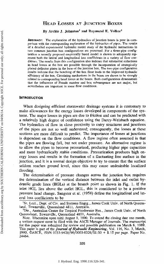
FIG. 1. Three Pipe Experimental Setup

K2 =

Ki =

'Ap2

7

Yl 2g

y

Yl 2g

(i)

(2)

where Ap/y is the pressure head change, g is the gravitational constant, and Vi is the mean velocity in the outlet pipe. Another feature of considerable interest is the position of the free surface in the box and this can be rep­resented as

Kw — 'WSEN

~vT 2g

(3)

in which WSE = the distance between the water surface and the downstream HGL intersection point at the branch point in the box.

Sangster et al. (1958) suggest appropriate head loss coefficients to be used when designing common junction box configurations. For example, the losses for a square box with two inlets and one outlet, as shown in Fig. 1, can be represented by the empirical relationships

Ki — Kn 1 -Qidt

2,4 (4)

and

327

J. Hydraul. Eng. 1990.116:326-341.

Dow

nloa

ded

from

asc

elib

rary

.org

by

SOU

TH

ER

N C

AL

IFO

RN

IA U

NIV

ER

SIT

Y o

n 04

/06/

14. C

opyr

ight

ASC

E. F

or p

erso

nal u

se o

nly;

all

righ

ts r

eser

ved.

K, Ki 1 Qid,

MiM-i

J J (5)

where # (for Z all flow is through the lateral pipe) = the loss coefficient, Q = flow rate, d = the diameter of the pipe, and subscripts 1,2, and 3 refer to the outlet, longitudinal, and lateral pipes, respectively.

Laboratory experimental studies completed by Blaisdell and Manson (1967) showed that these losses are fairly predictable where the pipe junction is of a closed tee configuration. Townsend and Prins (1978) carried out tests under nonpressurized conditions and suggest that benching the bottom of pits can significantly reduce energy losses. The results of detailed tests involving surcharged rectangular and circular boxes with "straight-through" flows are presented by Archer et al. (1978), who indicate that junction box geometry has the main influence on the coefficients. For the "straight-through" con­figuration, Marsalek (1984) concludes that for both circular and square pits a reduction in head loss is possible through floor benching.

The popularity of the square box configuration led Hare (1983) to develop a general semi-empirical equation to describe the distribution of head loss coefficients in a two-pipe junction as

K2 = 2 1 ARX

AR2

cos 62 (6)

and for a three-pipe junction as

Mr,\ (Q3 Ar\ K2 = K3 = 2 - 2 — cos G2 + 4 — — cos 92

/cos 93 cos 82 -lArx\ - + Ar3 Ar2

(7)

where the outlet pipe axis makes angles of 02 and 83 with the longitudinal and lateral pipe axes, respectively, and Ar is the area of the pipe. He then conducted a series of experiments to validate the two-pipe predictions; the results showed that Eq. 6 gave an adequate representation of the loss coef­ficients.

Lindval (1984) investigated circular manholes with a two-inlet-one-outlet pipe configuration. He found that the loss coefficients in a benched situation did vary with depth of water in the junction box and also with flow velocity. The losses were largest when the depth in the junction box was small and when significant swirling and water surface oscillations were observed.

Similar conclusions were reached by Howarth and Saul (1984), who con­sidered "straight-through" benched conditions for both circular and square boxes. It is believed that the reason for the difference between some of the conclusions reached by the final two research groups and previous research­ers is that longer inlet pipes were used in the more recent studies and this improved the developed velocity profiles along the pipes, resulting in more accurate hydraulic grade line and head loss determination.

Significant progress in urban drainage research has also been made through the development of computer programs. Two classes of models have been developed, a kinematic wave simulation type [e.g., ILLUDAS (Terstriep and Stall 1974)] and a dynamic wave simulation type [e.g., EXTRAN (Roesner

328

J. Hydraul. Eng. 1990.116:326-341.

Dow

nloa

ded

from

asc

elib

rary

.org

by

SOU

TH

ER

N C

AL

IFO

RN

IA U

NIV

ER

SIT

Y o

n 04

/06/

14. C

opyr

ight

ASC

E. F

or p

erso

nal u

se o

nly;

all

righ

ts r

eser

ved.

et al. 1981)1. Both are currently used in practice and their arrival has pro­duced a major step forward in urban drainage analysis and design. These programs have to be used with great care. Jacobsen and Harremoes (1984) conducted a field study and found that the dynamic wave programs (EX-TRAN and SI IS) gave reasonable results, while the kinematic wave pro­gram did not. They emphasize that the models are very sensitive to the as­sumed head loss parameters.

EXPERIMENTAL FACILITIES

Because a free water surface exists in the junction box, gravity is the dominant force and dynamic similarity is satisfied if model and prototype Froude numbers are equal. Since the hydraulic grade line and the total en­ergy line can be expressed in terms of length, model results can be directly scaled up by a length ratio (prototype length/model length). The loss coef­ficients are dimensionless. Prototype conditions indicate that pipe sizes are normally greater than 375 mm and that velocities between 0.5 and 6.0 m s_1 are commonly encountered in practice. Using these values the model geometry and flow condition ranges were established. Since energy losses in the pit are associated with turbulent eddies, similar levels of turbulence should be present in both prototype and model, which implies that the cor­responding Reynolds number, the relative roughness, and the friction factor ratios should be equal. Using a Froudian model, however, implies that the Reynolds number ratio should be the length ratio to the power 1.5, which in terms of a Moody-diagram-type relationship gives slightly smaller friction factor values for the model than required. This problem was overcome in the present situation by making the inside of the pit model smoother than dictated by scaling considerations and this was achieved by making the box from smooth acrylic sheet.

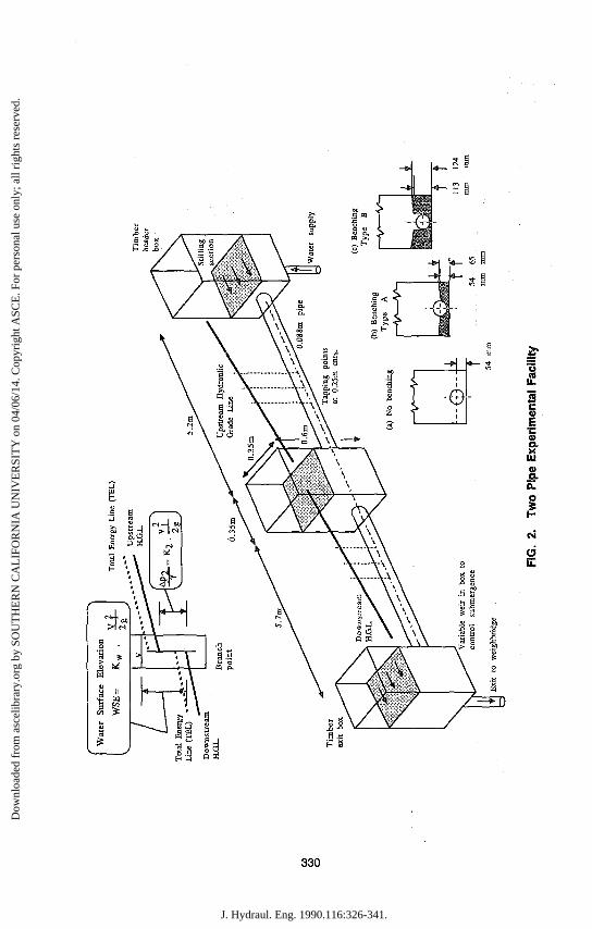
Fig. 1 illustrates the three-pipe experimental facility. Water pumped to the header boxes was supplied in a controlled and measurable manner through the use of valves and orifice plates. Reflecting typical prototype conditions, clear acrylic pipes of different diameter and length with equally spaced pi-ezometric tapping points were utilized. The square junction box (0.16 X 0.16 X 0.55-m deep) and the outlet control box were made from clear acrylic sheet. To investigate the head losses produced by streamlining the geometric conditions at the base of the junction box, clear acrylic deflectors were made and incorporated as shown in Fig. 1.

Although the initial runs were completed with length/diameter ratios of greater than 35.0, consistent with those used by Sangster et al. (1958), these ratios were increased to 68.0 to improve the quality of the HGL determi­nation. At the same time as this upgrade, other refinements were made; namely, the spacing between piezometric tapping points was reduced from 0.4 to 0.2 m and the entries of the pipes from the header boxes were bell-mouthed. Each of the configurations was tested at four flow rates and for each flow rate the losses were measured at six nominal ratios; i.e., Q3 (lateral flow rateVe, (outlet flow rate) = 0.0, 0.2, 0.4, 0.6, 0.8, and 1.0. To quantify the general influence of water depth in the junction box (submergence) on losses, runs at each of these conditions were completed at two different junc­tion box depths.

The layout of the "straight-through" two-pipe laboratory system is shown

329

J. Hydraul. Eng. 1990.116:326-341.

Dow

nloa

ded

from

asc

elib

rary

.org

by

SOU

TH

ER

N C

AL

IFO

RN

IA U

NIV

ER

SIT

Y o

n 04

/06/

14. C

opyr

ight

ASC

E. F

or p

erso

nal u

se o

nly;

all

righ

ts r

eser

ved.

co

CO

o

r 54

m

m

T

65

mm

113

mm

12

4 m

m

Exi

t to

w

eigh

brid

ge

FIG

. 2.

Tw

o Pi

pe E

xper

imen

tal

Faci

lity

J. Hydraul. Eng. 1990.116:326-341.

Dow

nloa

ded

from

asc

elib

rary

.org

by

SOU

TH

ER

N C

AL

IFO

RN

IA U

NIV

ER

SIT

Y o

n 04

/06/

14. C

opyr

ight

ASC

E. F

or p

erso

nal u

se o

nly;

all

righ

ts r

eser

ved.

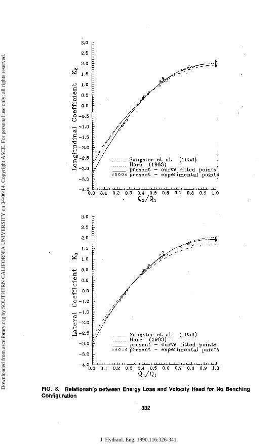
in Fig. 2. From the supply tank the water was fed to a timber header box then conveyed to and from the junction box by 0.088-m diameter clear acrylic pipes of lengths 5.2 m and 5.7 m, respectively. Piezometric tapping points were positioned at 0.25-m spacing in both pipes. The flow rate was mea­sured using a weighbridge system. The depth of surcharge in the box was controlled by a variable weir gate in the exit header box. The square junction box [0.35 X 0.35 X 0.60 m (height)] was made from timber with the front face from clear acrylic. The principal objectives of this second investigation were to study the effects of varying; benching arrangements at the base of the junction box, Froude number, and submergence. Fig. 2 illustrates the three configurations tested.

TREATMENT OF DATA

In both experimental facilities the HGL was determined from the water levels in the piezometric tubes. A linear least-squares-fit method was em­ployed to ensure consistency in measurement and analysis, the resulting cor­relation coefficients being 0.93, or better. In the two-pipe test program cor­relation coefficients of, on average, 0.95 were obtained at the lowest Froude number (0.04) while at Froude numbers above 0.13 the coefficients were all above 0.98. These high values were achieved even though the water surface fluctuations in the boxes were ±20 mm in some cases. There was evidence that in certain cases the pressures from tapping points in close proximity to the box were affected by local effects in the box but that their influence on the HGL fitted line was minimal due to the consideration of the many other experimental points along the pipe. This indicates that although the line-fitting procedure using all the tapping points seems consistent, there is some concern with the procedure that does not reflect the behavior of the pressure tappings close to the box, as these pressures would appear to be closely related to the actual energy loss mechanisms in the box. Further modifica­tions of the existing straight-line branch point method to reflect this localized behavior would seem appropriate.

Both junction box configurations have sharp edges; consequently it is be­lieved that Reynolds number effects will be of minor importance. This view is supported by Tuve and Sprenkle (1933), who concluded that for orifice-type flows the coefficient of contraction is virtually constant for flow situ­ations where Reynolds number is greater than 10,000. In the present tests the majority of flows satisfies this condition.

ANALYSIS OF RESULTS: THREE PIPE TESTS

Comparison with Previous Investigators In accordance with convention the results of the three-pipe study were

drawn in a graphical form (see Fig. 3) where the loss coefficients were plot­ted versus the lateral inlet to outlet flowrate ratio (23/<2i)- A nonlinear regression was performed using an International Mathematical and Statistics Library (1MSL) routine to determine least-squares-fitted equations of the form

M , o , * . = . + * ( ! ) + c ( ! ) 2+ D ( ! ) ' (8,

331

J. Hydraul. Eng. 1990.116:326-341.

Dow

nloa

ded

from

asc

elib

rary

.org

by

SOU

TH

ER

N C

AL

IFO

RN

IA U

NIV

ER

SIT

Y o

n 04

/06/

14. C

opyr

ight

ASC

E. F

or p

erso

nal u

se o

nly;

all

righ

ts r

eser

ved.

3.0

2.5

2.0 N

^ 1.5

-t-> 1,0 Pi .2 0.5 O

•r*

!£ °'° <D O -0.5 o _ -1.0 (S . a - i . 5 TS 3 -2.0

-i-> • F H

^ - 2 . 5

O ,_} -3.0

-3.5

-

; ': •

-•

-'. : -\ '-: : /, : // ~~Jf /

-_ /

'-

/ SA f'f

// ///

/,' /

a • n • a

-4.0

Sangs te r e t al . (1958) Hare (1983) p r e s e n t - curve f i t ted po in t s

annua p r e s e n t — e x p e r i m e n t a l po in t s

0.0 0.1 0.2 0.3 0.4 0.5 0.6 0.7 0.8 0.9 1.0 Q 3 / Q l

3.0

2.5

2.0

1.5

« l.o

*> 0.5 A £ o.o o

£ -0.5 <D O - 1 . 0 o

,-H -1.5

a!-2.0

2-2.5 -3.0 |

-3.5

-n.

i

r

r

r

t 0

//

/ /

a a a a

0.1 0.2

^rt^° — — ~" " a j ^ **

j v ^ ^

_ Sangs te r e t al . (1958) Hare (1983) p r e s e n t - curve f i t ted po in t s

a p r e s e n t - e x p e r i m e n t a l po in t s

' ' ' • 0.3 0.4 0.5 0.6 0.7 0.8 0.9 1.0

Q3/Qi

FIG. 3. Relationship between Energy Loss and Velocity Head for No Benching Configuration

332

J. Hydraul. Eng. 1990.116:326-341.

Dow

nloa

ded

from

asc

elib

rary

.org

by

SOU

TH

ER

N C

AL

IFO

RN

IA U

NIV

ER

SIT

Y o

n 04

/06/

14. C

opyr

ight

ASC

E. F

or p

erso

nal u

se o

nly;

all

righ

ts r

eser

ved.

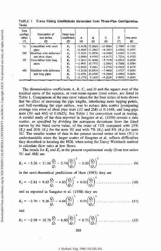
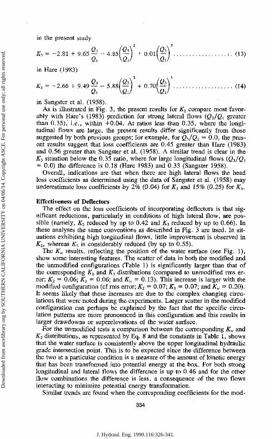
TABLE 1. Curve Fitting Coefficients Generated from Three-Pipe Configuration Tests

Test configu­ration

(1)

1U

2M

3U

4M

Description of test series

(2)

Unmodified with short pipes

Modified with deflectors and short pipes

Unmodified with long pipes

Modified with deflectors and long pipes

Head loss coefficient

(3)

K2

K,

K„

A

(4)

-3.4158 -2.4845 -3.3251 -2.0080 -3.2613 -2.9931 -2.8434 -3,2158 -2.4391 -2.1776

B

(5)

13.0963 11.2863 11.8078 9.9793

11.0096 10.7773 9.4861

10.8514 10.4500 9.1435

C

(6)

-10.4064 -9.1953 -8.9588 -8.4172 -5.7378 -6.5963 -3.2742 -7.4846 -9.2640 -6.2026

D

(7)

2.7080 2.4202 2.0383 1.7234

-0.0512 0.7088

-0.9463 1.4767 2.4906 0.9902

rms error

(8)

0.1222 0.1933 0.1118 0.1520 0.0596 0.0584 0.1274 0.0665 0.0656 0.2010

The dimensionless coefficients A, B, C, and D and the square root of the residual sums of the squares, or root-mean-square (rms) errors, are listed in Table 1. Comparison of the rms error values for the four series of tests shows that the effect of increasing the pipe lengths, introducing more tapping points, and bell-mouthing the pipe entries, was to reduce data scatter [comparing average rms error of short pipe tests (1U and 2M) of 0.1448, and long-pipe tests (3U and 4M) of 0.0625]. See Table 1 for convention used in testing. A careful study of the data reported in Sangster et al. (1958) reveals a data scatter, as specified by dividing the maximum deviations from the fitted curves by the fitted curve value, of the order of 12% compared with 15% (K2) and 20% (K3) for the tests 1U and with 7% (K2) and 8% (K3) for tests 3U. The smaller scatter of data in the present second series of tests (3U) is understandable since the larger scatter of Sangster et al. reflects difficulties they described in locating the HGL when using the Darcy Weisbach method to calculate flow rates at low flows.

The trends for K2 and K3 in the present experimental study (from test series 3U and 4M) are

K2 = -3.26 + 11.00 — - 5.74| —) - 0.05| — | (9)

in the semi-theoretical predictions of Hare (1983) they are

K2 = -2.81 + 9.65 — - 4.85( —) + 0.0l( —) (10)

and as reported in Sangster et al. (1958) they are

K2 = -2.70 + 9.26 — - 4.66( — ) + 0.0l( —) (11)

and

#3 = -2.99 + 10.78 — - 6.60| —J + 0.7l( — | (12)

333

• J. Hydraul. Eng. 1990.116:326-341.

Dow

nloa

ded

from

asc

elib

rary

.org

by

SOU

TH

ER

N C

AL

IFO

RN

IA U

NIV

ER

SIT

Y o

n 04

/06/

14. C

opyr

ight

ASC

E. F

or p

erso

nal u

se o

nly;

all

righ

ts r

eser

ved.

in the present study

K3 = -2.81 + 9.65 — - 4.851— ] + O.Olf — ) , . (13) (2i \QJ \QJ

in Hare (1983)

Z3 = -2.66 + 9.49 — - 5.881 —) + 0.70( —) (14)

in Sangster et al. (1958). As is illustrated in Fig. 3, the present results for K2 compare most favor­

ably with Hare's (1983) prediction for strong lateral flows (Q3/Qi greater than 0.35), i.e., within +0.04. At ratios less than 0.35, where the longi­tudinal flows are large, the present results differ significantly from those suggested by both previous groups; for example, for Q3/Q1 = 0.0, the pres­ent results suggest that loss coefficients are 0.45 greater than Hare (1983) and 0.56 greater than Sangster et al. (1958). A similar trend is clear in the K3 situation below the 0.35 ratio, where for large longitudinal flows (Q3/Q1 = 0.0) the difference is 0.18 (Hare 1983) and 0.33 (Sangster 1958).

Overall, indications are that when there are high lateral flows the head loss coefficients as determined using the data of Sangster et al. (1958) may underestimate loss coefficients by 2% (0.04) for K2 and 15% (0.25) for #3.

Effectiveness of Deflectors The effect on the loss coefficients of incorporating deflectors is that sig­

nificant reductions, particularly in conditions of high lateral flow, are pos­sible (namely, K2 reduced by up to 0.42 and K3 reduced by up to 0.66). In these analyses the same conventions as described in Fig. 3 are used. In sit­uations exhibiting high longitudinal flows, little improvement is observed in K2, whereas K3 is considerably reduced (by up to 0.55).

The Kw results, reflecting the position of the water surface (see Fig. 1), show some interesting features. The scatter of data in both the modified and the unmodified configurations (Table 1) is significantly larger than that of the corresponding K2 and K3 distributions (compared to unmodified rms er­ror; K2 = 0.06; K3 = 0.06; and Kw = 0.13). This increase is larger with the modified configuration (cf rms error; K2 = 0.07; K3 = 0.07; and K„ = 0.20). It seems likely that these increases are due to the complex changing circu­lations that were noted during the experiments. Larger scatter in the modified configuration can perhaps be explained by the fact that the specific circu­lation patterns are more pronounced in this configuration and this results in larger drawdowns or superelevations of the water surface.

For the unmodified tests a comparison between the corresponding Kw and K2 distributions, as represented by Eq. 8 and the constants in Table 1, shows that the water surface is consistently above the upper longitudinal hydraulic grade intersection point. This is to be expected since the difference between the two at a particular condition is a measure of the amount of kinetic energy that has been transformed into potential energy at the box. For both strong longitudinal and lateral flows the difference is up to 0.46 and for the other flow combinations the difference is less, a consequence of the two flows interacting to minimize potential energy transformation.

Similar trends are found when the corresponding coefficients for the mod-

334

J. Hydraul. Eng. 1990.116:326-341.

Dow

nloa

ded

from

asc

elib

rary

.org

by

SOU

TH

ER

N C

AL

IFO

RN

IA U

NIV

ER

SIT

Y o

n 04

/06/

14. C

opyr

ight

ASC

E. F

or p

erso

nal u

se o

nly;

all

righ

ts r

eser

ved.

ified box are compared. In the case of K2 the difference between the K? and the Kw values appears to be almost indirectly dependent on the Q3/Qt ratio as it increases from 0.13 at Q3/Qi = 1.0 to 1.04 at Q3/Qi = 0.0. In contrast, the difference between K3 and Kw changes in the opposite direction with a difference of 0.52 at Q3/Ql = 1.0 and 0.26 at G3/G1 = 0.0. Comparing the corresponding modified and the unmodified K„ values a trend similar to that of the K2 and K3 patterns emerges, i.e., the loss values are considerably reduced by using deflector plates.

Effects of Submergence For various submergence ratios the results for both the unmodified and

modified configurations were determined using the aforementioned proce­dure. In this analysis four submergence ratios (depth of water in the box/ outlet pipe diameter) were selected for comparison, i.e., (1.0-2.0), (2.0-3.0), (3.0-4.0) and (4.0-5.6). The three head loss coefficients in these ranges were then least-squares-curve-fitted using a third-order polynomial and the representative coefficients at Q3/Qi ratios of: 0.0, 0.2, 0.4, 0.6, 0.8, and 1.0 were compared. In both K2 cases (unmodified and modified) with large longitudinal flows there is a relatively small change in value (up to ~0.08) with large changes in submergence. With large lateral flows there is a con­siderable decrease in their value (—0.25) with increase in submergence. The trend with K3 for both box configurations is different; at high longitudinal flows with the unmodified case there is a higher variation in values (0.16) than with the modified case (0.02). These values seem to increase and then decrease with submergence. With stronger lateral flows the maximum dif­ferences recorded for both configurations are considerably greater (unmodi­fied 0.24, modified 0.19) compared with those for the larger longitudinal flows. There is again a tendency for the K3 values to decrease as submer­gence is increased.

Effects of Froude Number To investigate the influence of Froude number, the results were sorted

into three nominal groups, i.e., Froude number = 0.22, 0.44, and 0.63. Least-squares-fitted curves were then established and representative results compared.

Differences in K2 for large longitudinal flows are relatively small (e.g., 0.07) compared to the strong lateral flows (e.g., 0.20); however, at these large lateral flows the unmodified coefficients decrease with increase in Froude number while with modified configuration there is no clear trend. K3 losses with both the unmodified and modified configurations increase marginally with Froude number for both large longitudinal and large lateral flows. This pattern is also apparent in the K„ case for all these four situations with the changes being greater than for K3 (compared to K3, 0.11; K„, 0.28, where these values represent averages of maximum differences).

ANALYSIS OF RESULTS: TWO PIPE TESTS

General From the three pipe test program it was clear that submergence and Froude

number (F) were important parameters. Recent research has investigated some of the aspects of junction box hydraulics when the floor of the box is benched

335

J. Hydraul. Eng. 1990.116:326-341.

Dow

nloa

ded

from

asc

elib

rary

.org

by

SOU

TH

ER

N C

AL

IFO

RN

IA U

NIV

ER

SIT

Y o

n 04

/06/

14. C

opyr

ight

ASC

E. F

or p

erso

nal u

se o

nly;

all

righ

ts r

eser

ved.

(or molded) but a detailed understanding of the fluid interactions produced by different types of benching under these conditions is not available.

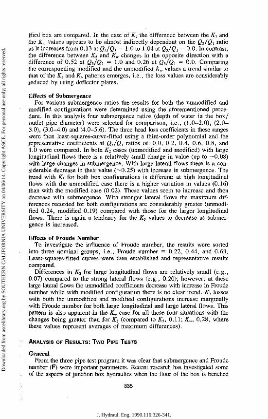
A study was completed for three typical junction bottom benching con­figurations (including no benching), six Froude numbers, and up to six sub­mergence depths. In addition to pressure tapping measurements along the pipes, a careful observation of the different circulation patterns for the dif­ferent flow conditions was recorded. Some of the results are presented in Table 2, which describes a number of interesting features. The head loss K2

appeared to vary with submergence, Froude number, and the type of bench­ing used. At some of the lower Froude numbers there was evidence to sug­gest that a pattern exists where initially the losses are small but increase until submergence is close to 1.5, then reduce again with submergence in­crease.

For all the submergences, an increase in Froude number generally pro­duces a decrease in losses and this may be illustrated by comparing the losses for the no-benching configuration at submergences greater than 3.5, e.g., F = 0.04 K2 = 1.78; F = 0.18 K2 = 0.81; F = 0.31 K2 = 0.49; F = 0.78 K2 = 0.38.

Benching The effect of benching also has a pronounced effect on the losses, e.g.,

when F = 0.04 no benching, Ki = 1.78; benching type A, K2 = 1.64; benching type B, K2 = 1.04. When F = 0.75 no benching, K2 = 0.38; benching type A, K2 = 0.26; benching type B, K2 = 0.24.

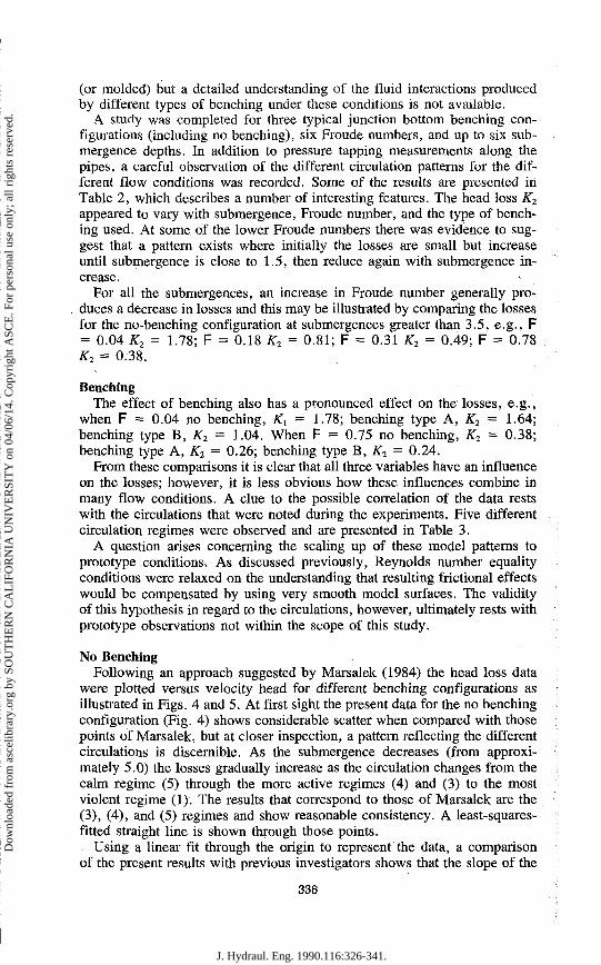
From these comparisons it is clear that all three variables have an influence on the losses; however, it is less obvious how these influences combine in many flow conditions. A clue to the possible correlation of the data rests with the circulations that were noted during the experiments. Five different circulation regimes were observed and are presented in Table 3.

A question arises concerning the scaling up of these model patterns to prototype conditions. As discussed previously, Reynolds number equality conditions were relaxed on the understanding that resulting frictional effects would be compensated by using very smooth model surfaces. The validity of this hypothesis in regard to the circulations, however, ultimately rests with prototype observations not within the scope of this study.

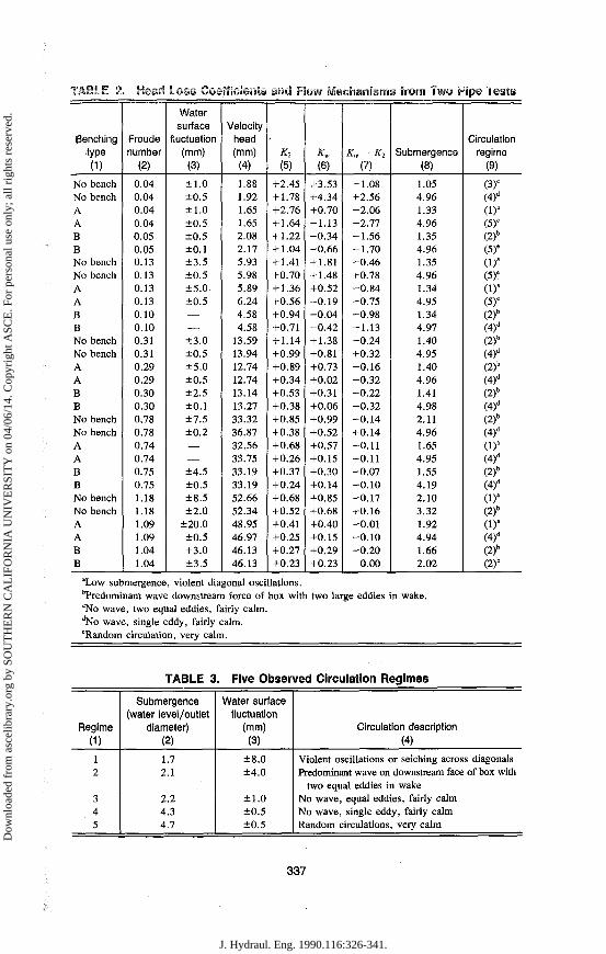
No Benching Following an approach suggested by Marsalek (1984) the head loss data

were plotted versus velocity head for different benching configurations as illustrated in Figs. 4 and 5. At first sight the present data for the no benching configuration (Fig. 4) shows considerable scatter when compared with those points of Marsalek, but at closer inspection, a pattern reflecting the different circulations is discernible. As the submergence decreases (from approxi­mately 5.0) the losses gradually increase as the circulation changes from the calm regime (5) through the more active regimes (4) and (3) to the most violent regime (1). The results that correspond to those of Marsalek are the (3), (4), and (5) regimes and show reasonable consistency. A least-squares-fitted straight line is shown through those points.

Using a linear fit through the origin to represent the data, a comparison of the present results with previous investigators shows that the slope of the

336

J. Hydraul. Eng. 1990.116:326-341.

Dow

nloa

ded

from

asc

elib

rary

.org

by

SOU

TH

ER

N C

AL

IFO

RN

IA U

NIV

ER

SIT

Y o

n 04

/06/

14. C

opyr

ight

ASC

E. F

or p

erso

nal u

se o

nly;

all

righ

ts r

eser

ved.

TASLE 2. Head Loss Coefficients and Fiow Mechanisms from Two Pipe 'fests

Benching type

(1)

No bench No bench A A B B No bench No bench A A B B No bench No bench A A B B No bench No bench A A B B No bench No bench A A B B

Froude number

(2)

0.04 0.04 0.04 0.04 0.05 0.05 0.13 0.13 0.13 0.13 0.10 0.10 0.31 0.31 0.29 0.29 0.30 0.30 0.78 0.78 0.74 0.74 0.75 0.75 1.18 1.18 1.09 1.09 1.04 1.04

Water surface

fluctuation (mm)

(3)

±1.0 ±0.5 ±1.0 ±0.5 ±0.5 ±0.1 ±3.5 ±0.5 ±5.0 ±0.5

— — ±3.0 ±0.5 ±5.0 ±0.5 ±2.5 ±0.1 ±7.5 ±0.2

— — ±4.5 ±0.5 ±8.5 ±2.0

±20,0 ±0,5 +3.0 ±3,5

Velocity head (mm)

(4)

1.88 1.92 1.65 1.65 2.08 2.17 5.93 5.98 5.89 6.24 4.58 4.58

13.59 13.94 12.74 12.74 13.14 13.27 33.32 36.87 32.56 33.75 33.19 33.19 52.66 52.34 48.95 46.97 46.13 46.13

K2

(5)

+2.45 + 1.78 +2.76 + 1.64 + 1.22 + 1.04 + 1.41 +0.70 + 1.36 +0.56 +0.94 +0.71 + 1.14 +0.99 +0.89 +0.34 +0.53 +0.38 +0.85 +0.38 +0.68 +0.26 +0.37 +0.24 +0.68 +0.52 +0.41 +0.25 +0.27 +0.23

Kw

(6)

+3,53 +4.34 +0.70 -1 .13 -0 .34 - 0 . 6 6 + 1.81 + 1.48 +0.52 - 0 . 1 9 -0 .04 - 0 . 4 2 + 1.38 +0.81 +0.73 +0.02 +0.31 +0.06 +0.99 +0.52 +0.57 +0.15 +0.30 +0.14 +0.85 +0.68 +0.40 +0.15 +0.29 +0.23

K„ - K2

(7)

+ 1.08 +2.56 -2 .06 -2 .77 -1 .56 -1 .70 +0.46 +0.78 -0 .84 -0 .75 -0 .98 -1 .13 +0.24 +0.32 -0 .16 -0 .32 -0 .22 -0 .32 +0.14 +0.14 -0 .11 -0 .11 -0 .07 -0 .10 +0.17 +0.16 -0 .01 -0 .10 +0.20

0.00

Submergence

(8)

1.05 4.96 1.33 4.96 1.35 4.96 1.35 4.96 1.34 4.95 1.34 4.97 1.40 4.95 1.40 4.96 1.41 4.98 2.11 4.96 1.65 4.95 1.55 4.19 2.10 3.32 1.92 4.94 1.66 2.02

Circulation regime

(9)

(3)c

(4)" (1)" (5)s

(2)b

(5)e

(Da

(5)' (1)" (5)e

(2)b

(4)d

(2)b

(4)" (2)b

(4)d

(2)b

(4)" (2)b

(4)" (1)'

(4)d

(2)b

(4)d

(1)' (2)b

(1)" (4)d

(2)b

(2)b

"Low submergence, violent diagonal oscillations. bPredominant wave downstream force of box with two large eddies in wake. 'No wave, two equal eddies, fairly calm. dNo wave, single eddy, fairly calm. 'Random circulation, very calm.

TABLE 3. Five Observed Circulation Regimes

Regime

(1)

1 2

3 4 5

Submergence (water level/outlet

diameter)

(2)

1.7 2.1

2.2 4.3 4.7

Water surface fluctuation

(mm)

(3)

±8.0 ±4.0

±1.0 ±0.5 ±0.5

Circulation description

(4)

Violent oscillations or seiching across diagonals Predominant wave on downstream face of box with

two equal eddies in wake No wave, equal eddies, fairly calm No wave, single eddy, fairly calm Random circulations, very calm

337

J. Hydraul. Eng. 1990.116:326-341.

Dow

nloa

ded

from

asc

elib

rary

.org

by

SOU

TH

ER

N C

AL

IFO

RN

IA U

NIV

ER

SIT

Y o

n 04

/06/

14. C

opyr

ight

ASC

E. F

or p

erso

nal u

se o

nly;

all

righ

ts r

eser

ved.

Regimes (1) and (2)

Regimes (3),(4) and (5)

0 10 20 30 40 50 60 [0] [0.22] [0.45] [0.67] [0.90] [1.12] [1.35]

Veloc i ty Head , V^ / 2g (mm)

[Froude Number ]

Key

(1) Violent oscillations, very turbulent

(2) Wave on downstream face, two eddies, fairly turbulent

(3) No wave, two eddies, fairly turbulent

(4) No wave, one eddy, fairly calm

(5) Random circulations, very calm

FIG. 4. Head Loss Data versus Velocity Head for No Bending Configuration

line is approximately dependent on the size of the box, as shown in Ta­ble 4.

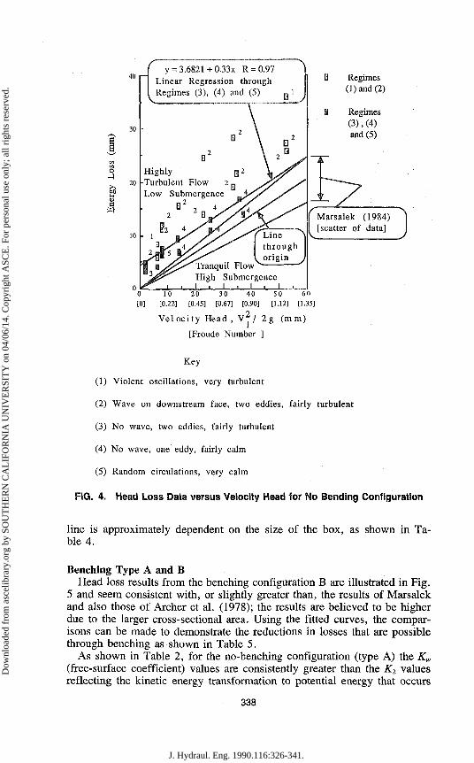
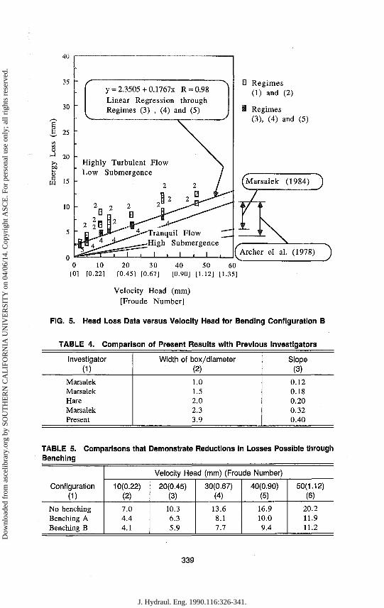
Benching Type A and B Head loss results from the benching configuration B are illustrated in Fig.

5 and seem consistent with, or slightly greater than, the results of Marsalek and also those of Archer et al. (1978); the results are believed to be higher due to the larger cross-sectional area. Using the fitted curves, the compar­isons can be made to demonstrate the reductions in losses that are possible through benching as shown in Table 5.

As shown in Table 2, for the no-benching configuration (type A) the K„ (free-surface coefficient) values are consistently greater than the K2 values reflecting the kinetic energy transformation to potential energy that occurs

338

J. Hydraul. Eng. 1990.116:326-341.

Dow

nloa

ded

from

asc

elib

rary

.org

by

SOU

TH

ER

N C

AL

IFO

RN

IA U

NIV

ER

SIT

Y o

n 04

/06/

14. C

opyr

ight

ASC

E. F

or p

erso

nal u

se o

nly;

all

righ

ts r

eser

ved.

0 Regimes (1) and (2)

i Regimes (3), (4) and (5)

10 20 30 40 50 60 [0.22] [0.45] [0.67] [0.90] [1.12] [1.35]

Velocity Head (mm)

[Froude Number]

fArcher el al. (1978) )

FIG. 5. Head Loss Data versus Velocity Head for Bending Configuration B

TABLE 4. Comparison of Present Results with Previous Investigators

Investigator

(1)

Marsalek Marsalek Hare Marsalek Present

Width of box/diameter (2)

1.0 1.5 2.0 2.3 3.9

Slope (3)

0.12 0.18 0.20 0.32 0.40

TABLE 5. Comparisons that Demonstrate Reductions in Losses Possible through Benching

Configuration

0) No benching Benching A Benching B

Velocity Head (mm) (Froude Number)

10(0.22) (2)

7.0 4.4 4.1

20(0.45) (3)

10.3 6.3 5.9

30(0.67) (4)

13.6 8.1 7.7

40(0.90) (5)

16.9 10.0 9.4

50(1.12) (6)

20.2 11.9 11.2

339

J. Hydraul. Eng. 1990.116:326-341.

Dow

nloa

ded

from

asc

elib

rary

.org

by

SOU

TH

ER

N C

AL

IFO

RN

IA U

NIV

ER

SIT

Y o

n 04

/06/

14. C

opyr

ight

ASC

E. F

or p

erso

nal u

se o

nly;

all

righ

ts r

eser

ved.

as the water passes through the box. The magnitude of this varies, on av­erage, from 1.5 at a low Froude number (F) of 0.04 down to —0.13 at F 1.18. The conversion of kinetic to potential energy is greatest when the fluid in the box is tranquil, while when the water is mixing violently this con­version rate is decreased and the water level drops.

CONCLUSION

Results from an experimental three-pipe junction box facility confirm that a proposed empirically based model can be used to represent both the lateral and longitudinal loss coefficients for a variety of flow conditions.

Results also suggest that significant improvements to the hydraulic effi­ciency of such boxes can be realized if deflector (or baffle) plates are in­corporated in the box. Although the influences of box submergence and Froude number are not major they are nevertheless important in some flow situa­tions.

Experimental evidence from a two pipe junction box investigation suggests that benching of the box floor leads to a general reduction of losses and promotes improved hydraulic efficiency. It is also suggested that the cir­culating mechanisms, or regimes, in these boxes are strongly related to the corresponding head losses in the boxes.

ACKNOWLEDGMENTS

These experiments were undertaken in the Department of Civil and Sys­tems Engineering at James Cook University and the Department of Civil Engineering at Manchester University. Partial support was provided by the Special Research Grants programs of James Cook University and of Wol-longong University.

APPENDIX I. REFERENCES

Archer, B., Bettess, F., and Colyer, P. J. (1978). "Head loss and air entrainment at sewer manholes." Report IT 185, Hydraulics Research Station, Wallingford, England.

Blaisdell, F. W., and Manson, P. W. (1967). "Energy losses at pipe junctions." J. Hydr. Div., ASCE, 76(3), 57-78.

Hare, C. M. (1983). "Magnitude of hydraulic losses at junctions in piped drainage systems." Civil Engineering Trans., Institution of Engineers, 25(1), 71-77.

Howarth, D. A., and Saul, A. J. (1984). "Energy loss coefficients at manholes." Proc. 3rd Int. Conf. on Urban Storm Drainage, 1, 127-136.

Jacobsen, P., and Harremoes, P. (1984). "The significance of head loss parameters in surcharged sewer simulations." Proc. 3rd Int. Conf. on Urban Drainage, 1, 167-176.

Johnston, A. J., Pettigrew, M. R., and Volker, R. E. (1987). "Energy losses in a surcharged three pipe stormwater pit." Proc. Conf. on Hydr. in Civ. Engrg., In­stitution of Engineers, 100-104.

Lindval, G. (1984). "Head losses at surcharged manholes with a main pipe and a 90° lateral." Proc. 3rd Int. Conf. on Urban Drainage, 1, 137-146.

Marsalek, J. (1984). "Head losses at sewer junction manholes." J. Hydr. Engrg., ASCE, 110(8), 1150-1154.

Roesner, L. A., Shubinski, R. P., and Aldrich, J. A. (1981). "Stormwater man­agement model users' manual—version HI, addendum I—EXTRAN." Report No. EPA-600/2, U.S. Environmental Protection Agency, Washington, D.C., 84-109.

340

J. Hydraul. Eng. 1990.116:326-341.

Dow

nloa

ded

from

asc

elib

rary

.org

by

SOU

TH

ER

N C

AL

IFO

RN

IA U

NIV

ER

SIT

Y o

n 04

/06/

14. C

opyr

ight

ASC

E. F

or p

erso

nal u

se o

nly;

all

righ

ts r

eser

ved.

Sangster, W. M., et al. (1958). "Pressure changes at storm drain junctions. Bulletin No. 41, Engineering Experimental Station, Univ. of Missouri, Columbia, Mo.

Terstriep, M. C , and Stall, J. B. (1974). "The Illinois urban drainage area simulator ILLUDAS." Bulletin 58, Illinois State Water Survey, Urbana, 111.

Townsend, R. D., and Prins, J. R. (1978). "Performance of model stormsewer junc­tions." J. Hydr. Div., ASCE, 104(1), 99-104.

Tuve, G. L., and Sprenkle, R. E. (1933). "Orifice discharge coefficients for viscous liquids." Instruments, 6, 201.

APPENDIX II. NOTATION

The following symbols are used in this paper:

A = coefficient used in curve-fitting procedure; Ar = area of pipe; B = coefficient used in curve-fitting procedure; C = coefficient used in curve-fitting procedure; D = coefficient used in curve-fitting procedure; d = diameter of pipe; F = Froude number = Vi/Q^ii g = gravitational acceleration; K = head-loss coefficient = Ap • 2g/yVi; K = head-loss coefficient with all flow through lateral pipe;

Ap = pressure change; Q = flow rate; V = mean velocity in pipe;

WSE = water surface elevation; 7 = specific weight of water; and 8 = angle between upstream and downstream pipes.

Subscripts 1 = 2 = 3 =

outlet pipe; inlet longitudinal pipe; inlet lateral pipe; and water surface.

341

J. Hydraul. Eng. 1990.116:326-341.

Dow

nloa

ded

from

asc

elib

rary

.org

by

SOU

TH

ER

N C

AL

IFO

RN

IA U

NIV

ER

SIT

Y o

n 04

/06/

14. C

opyr

ight

ASC

E. F

or p

erso

nal u

se o

nly;

all

righ

ts r

eser

ved.