hanford sludge simulant selection for soil mechanics ... · hanford sludge simulant selection for...
TRANSCRIPT

PNNL-19250
Prepared for the U.S. Department of Energy under Contract DE-AC05-76RL01830
Hanford Sludge Simulant Selection for Soil Mechanics Property Measurement BE Wells GN Brown EC Golovich RL Russell DE Rinehart JV Crum LA Mahoney WC Buchmiller March 2010
DISCLAIMER This report was prepared as an account of work sponsored by an agency of the United States Government. Neither the United States Government nor any agency thereof, nor Battelle Memorial Institute, nor any of their employees, makes any warranty, express or implied, or assumes any legal liability or responsibility for the accuracy, completeness, or usefulness of any information, apparatus, product, or process disclosed, or represents that its use would not infringe privately owned rights. Reference herein to any specific commercial product, process, or service by trade name, trademark, manufacturer, or otherwise does not necessarily constitute or imply its endorsement, recommendation, or favoring by the United States Government or any agency thereof, or Battelle Memorial Institute. The views and opinions of authors expressed herein do not necessarily state or reflect those of the United States Government or any agency thereof. PACIFIC NORTHWEST NATIONAL LABORATORY operated by BATTELLE for the UNITED STATES DEPARTMENT OF ENERGY under Contract DE-ACO5-76RL01830
Printed in the United States of America
Available to DOE and DOE contractors from the Office of Scientific and Technical Information,
P.O. Box 62, Oak Ridge, TN 37831-0062; ph: (865) 576-8401 fax: (865) 576 5728
email: [email protected]
Available to the public from the National Technical Information Service, U.S. Department of Commerce, 5285 Port Royal Rd., Springfield, VA 22161
ph: (800) 553-6847 fax: (703) 605-6900
email: [email protected] online ordering: http://www.ntis.gov/ordering.htm
PNNL-19250
Hanford Sludge Simulant Selection for Soil Mechanics Property Measurement BE Wells GN Brown EC Golovich RL Russell DE Rinehart JV Crum LA Mahoney WC Buchmiller March 2010 Prepared for the U.S. Department of Energy under Contract DE-AC05-76RL01830 Pacific Northwest National Laboratory Richland, Washington

iii
Summary
This report describes current work to select or develop two chemical sludge simulants for testing relative to problems of hydrogen gas retention and release encountered in the double shell tanks at the Hanford Site near Richland, Washington. Wastes from single shell tanks are being transferred to double shell tanks for safety reasons (some single shell tanks are leaking or are in danger of leaking), but the available double-shell tank space is limited.
The current System Plan for the Hanford Tank Farms (Rev. 4, Certa and Wells 2009) uses relaxed buoyant displacement gas release event (BDGRE) controls for deep sludge (i.e., high level waste [HLW]) tanks, which allows the tank farms to use more storage space, i.e., increase the sediment depth, in some of the double-shell tanks (DSTs). The relaxed BDGRE controls are based on preliminary analysis of a gas release model from van Kessel and van Kesteren (2002). Application of the van Kessel and van Kesteren model requires parametric information for the sediment, including the lateral earth pressure at rest and shear modulus. No lateral earth pressure at rest and shear modulus in situ measurements for Hanford sludge are currently available.
The two chemical sludge simulants will be used in follow-on work to experimentally measure the van Kessel and van Kesteren (2002) model parameters, lateral earth pressure at rest, and shear modulus. The simulants are selected via similarity to measured Hanford sludge chemical and physical properties, including liquid density, viscosity, and pH, undissolved particle size and density, and slurry rheology to maximize the likelihood that the simulants will have similar lateral earth pressure at rest and shear modulus as Hanford sludge. Simulant 1 is selected from those Hanford sludge simulants that have previously been produced and characterized, and Simulant 2 is developed based upon the chemistry of a specific retrieval SST scenario. In Section 2, pertinent Hanford sludge properties are summarized, Simulant 1 is selected, and the chemistry for Simulant 2 is developed and presented. Simulant production is described in Section 3, and simulant property measurements are presented in Section 4. A summary is provided in Section 5.
Simulants 1 and 2 are shown to have chemical and physical properties that match well with all of the Hanford sludge parameters considered. The uniqueness of the simulants with respect to each other for some of the parameters considered is a beneficial outcome given the broad variation of Hanford waste.

v
Acronyms and Abbreviations
BBI Best Basis Inventory
BDGRE buoyant displacement gas release event
DST double-shell tank
EQL estimated quantification limit
ESP Environmental Simulation Program
HLW high-level waste
KOH potassium hydroxide
MDL method detection limit
PEP Pretreatment Engineering Platform
PNNL Pacific Northwest National Laboratory
PSD particle-size distribution
PSDD particle size and density distribution
REDOX reduction oxidation
RPP River Protection Project
SEM scanning electron microscopy
SST single-shell tank
TOC total organic carbon
UDS undissolved solids
WTP Hanford Tank Waste Treatment and Immobilization Plant
XRD X-ray diffraction

vii
Contents
Summary ............................................................................................................................................... iii
Acronyms and Abbreviations ............................................................................................................... v
1.0 Introduction .................................................................................................................................. 1.1
2.0 Simulant Selection ....................................................................................................................... 2.1
2.1 Hanford Sludge Properties .................................................................................................. 2.1
2.1.1 Liquid Properties ..................................................................................................... 2.1
2.1.2 Slurry Properties ..................................................................................................... 2.2
2.1.3 Hanford Sludge Waste Physical Property Summary .............................................. 2.11
2.2 Simulant 1 Selection ........................................................................................................... 2.12
2.3 Simulant 2 Selection: Sludge-of-Interest Chemistry .......................................................... 2.15
2.3.1 Use of ESP Model Predictions ................................................................................ 2.15
2.3.2 Combination of Inventories for the Four Tanks of Interest .................................... 2.17
3.0 Simulant Preparation .................................................................................................................... 3.1
3.1 Simulant 1 Preparation ....................................................................................................... 3.1
3.2 Simulant 2 Preparation ....................................................................................................... 3.3
4.0 Simulant Properties ...................................................................................................................... 4.1
4.1 Chemical Composition ....................................................................................................... 4.1
4.2 Liquid Properties ................................................................................................................ 4.11
4.3 Particle-Size Distribution .................................................................................................... 4.12
4.4 Rheology ............................................................................................................................. 4.13
4.5 Shear Modulus .................................................................................................................... 4.17
4.6 Settling ................................................................................................................................ 4.19
4.7 Particulate Imaging ............................................................................................................. 4.21
5.0 Summary ...................................................................................................................................... 5.1
6.0 References .................................................................................................................................... 6.1
Appendix A: Recipe for Simulant 1 Iron-Bearing and Supernatant Simulant Component Preparation ................................................................................................................................... A.1
Appendix B: Simulant 1 Preparation .................................................................................................... B.1
Appendix C: Recipe for Simulant 2 Preparation .................................................................................. C.1
Appendix D: Simulant 2 Liquid Viscosity Flow Curves ...................................................................... D.1
Appendix E: Simulant PSD Data .......................................................................................................... E.1
Appendix F: Simulant Slurry Rheology Flow Curves .......................................................................... F.1
viii
Figures
2.1. Hanford Liquid Density, all 177 Tanks ...................................................................................... 2.2
2.2. Hanford Liquid Density, all 81 Sludge Tanks ............................................................................ 2.3
2.3. Hanford Liquid Viscosity ........................................................................................................... 2.3
2.4. Hanford Sludge Tanks: Sediment UDS Volume and Mass Fractions ........................................ 2.5
2.5. Bingham Rheological Model Data for Slurries from 18 Hanford Sludge Tanks, Volume Fraction UDS .............................................................................................................................. 2.7
2.6. Bingham Rheological Model Data for Slurries from 18 Hanford Sludge Tanks, Mass Fraction UDS .............................................................................................................................. 2.8
2.7. Probabilities for Bingham Consistency for Slurries from 18 Hanford Sludge Tanks, Mass Fraction UDS .............................................................................................................................. 2.9
2.8. Probabilities for Bingham Yield Stress for Slurries from 18 Hanford Sludge Tanks, Mass Fraction UDS .............................................................................................................................. 2.9
2.9. Sediment Shear Strength Data for 16 Hanford Sludge Tanks, Volume Fraction UDS .............. 2.10
2.10. Sediment Shear Strength Data for 15 Hanford Sludge Tanks, Mass Fraction UDS .................. 2.10
2.11. Probabilities for Sediment Shear Strength Data for 15 Hanford Sludge Tanks, Mass Fraction UDS .............................................................................................................................. 2.11
4.1. Simulant 1 XRD Results with Peak Identification ..................................................................... 4.8
4.2. Simulant 2 XRD Results with Peak Identification ..................................................................... 4.9
4.3. Simulant 2 SEM EDS Elemental Analysis with Peak Identification.......................................... 4.10
4.4. Location of SEM Elemental Analysis for Simulant 2 ................................................................ 4.11
4.5. Simulant Bingham Parameters as Functions of Mass Fraction UDS ......................................... 4.14
4.6. Shear Strength as a Function of UDS Concentration ................................................................. 4.16
4.7. Shear Strength and Shear Modulus as a Function of UDS Concentration ................................ . 4.19
4.8. Simulant Settling Test Results .................................................................................................... 4.20
4.9. Calculated Simulant Settled Layer Shear Strength as a Function of Settling Time, Settling Data from 4.3 .............................................................................................................................. 4.21
4.10. SEM Micrographs, Simulant 1 (Geeting et al. 2009). Magnification—A: 1,000×, B: 2,500×, C: 5,000×, and D: 10,000×. ...................................................................................... 4.22
4.11. a) Gibbsite/Al(OH)3 from Tank AY-102,() b) Gibbsite/Al(OH)3 from Tank AZ-102 ................ 4.23
4.12. Boehmite/AlOOH Particles from Tank S-104 ............................................................................ 4.23
4.13. a) Fe2O3 from Tank C-101(); b) Fe2O3 from Tank AN-107 ........................................................ 4.24
4.14. SEM Micrographs, Simulant 2; a) Location 1, Magnification 1500×, b) Location 1, Magnification 5000×, c) Location 2, Magnification 1000× ....................................................... 4.25
4.15. a) ZrO2 from Tank AY-102(); b) ZrO2, from Tank SY-102 ........................................................ 4.26
ix
Tables
2.1. Case 3 PSDD (Wells et al. 2007) ............................................................................................... 2.6
2.2. Hanford Sludge Waste Properties Summary .............................................................................. 2.11
2.3. Simulant and Hanford Sludge Waste Properties Comparison .................................................... 2.13
2.4. ESP-Predicted Bulk Compositions for the Four Tanks .............................................................. 2.19
2.5. ESP-Predicted Liquid-Phase Compositions for the Four Tanks ................................................. 2.20
2.6. Four-Tank Waste Mixture Composition, from Summing ESP Predictions ................................ 2.21
2.7. Four-Tank Waste Primary (Mass Fraction >0.5) Solid Phase Compound Composition, from Summing ESP Predictions .......................................................................................................... 2.22
3.1. Postulated Composition of Iron-Rich Sludge ............................................................................. 3.2
3.2. Chemical Components Used to Produce Supernate Simulant .................................................... 3.2
4.1. Liquid Phase Composition, Simulant 1 ...................................................................................... 4.3
4.2. Liquid Phase Composition, Simulant 2 ...................................................................................... 4.4
4.3. Slurry Phase Composition, Simulant 1 ....................................................................................... 4.5
4.4. Slurry Phase Composition, Simulant 2 ....................................................................................... 4.6
4.5. Selected Postulated Primary UDS Solid Phase Compounds ...................................................... 4.7
4.6. Simulant 2 SEM EDS Elemental Analysis with Peak Quantification ........................................ 4.10
4.7. Liquid Properties ........................................................................................................................ 4.12
4.8. Volume-Based PSD Percentiles (m) ........................................................................................ 4.12
4.9. Bingham Rheological Parameters .............................................................................................. 4.14
4.10. Shear Strength ............................................................................................................................ 4.15
4.11. Bingham Yield Stress and Shear-Strength Comparison ............................................................. 4.17
4.12. Shear Modulus ............................................................................................................................ 4.19

1.1
1.0 Introduction
Radioactive wastes composed of liquid (water and dissolved solids) and settled undissolved solids (UDS) are stored in 177 large underground storage tanks on the Hanford Site. The 177 storage tanks include 149 single shell tanks (SSTs) and 28 double shell tanks (DSTs). Waste will be retrieved from the SSTs to interim storage in the DSTs. Certa and Wells (2009) (System Plan [Rev. 4]) report that the
Baseline Case, which, in part, describes how the River Protection Project (RPP) mission(a) could be achieved given an underlying set of assumptions, shows that there is adequate DST space to meet the near-term success criteria for specific SST retrieval. Subsequently, however, there will be minimal DST space available to proceed with additional SST retrievals. Management of DST space is thus a key issue.
The UDS management strategy in the previous System Plan (Rev. 3) followed the existing buoyant displacement gas release event (BDGRE) controls (Weber 2008). The depth of settled UDS or sediment accumulated in a DST, and therefore the inventory of UDS that may be stored in a DST, is limited by these controls.
Hanford radioactive wastes generate flammable gases (Weber 2008). Hydrogen is the primary flammable component of the generated gas (Meyer and Stewart 2001). Flammable gas generation by itself is not a hazard if the generated gas is released continuously as fast as it is generated. In some DST wastes, however, specifically those with deep layers of supernatant liquid and sediment (sediment - settled UDS and interstitial liquid), the generated gas can accumulate in the sediment until a portion of the sediment accumulates gas such that it becomes sufficiently buoyant to overcome its weight and the strength of the surrounding material restraining it. The sufficiently buoyant portion then rises through the supernate, and the resultant expansion of the retained gas yields the retaining material such that a fraction of the retained gas is released, and the remaining non-buoyant material sinks back to the sediment (e.g., Wells et al. 2002, Meyer and Stewart 2001, Hedengren et al. 2000). This gas release process defines a BDGRE.
The current System Plan (Rev. 4, Certa and Wells 2009) uses relaxed BDGRE controls for deep sludge (i.e., high level waste [HLW]) tanks, which allow the tank farms to use more storage space, i.e., increase the sediment depth, in some of the DSTs. The relaxed BDGRE controls are based on preliminary analysis of a gas release model from van Kessel and van Kesteren (2002). Applying the van Kessel and van Kesteren model requires parametric information for the sediment, including the undrained shear strength, void ratio, UDS and liquid density, lateral earth pressure at rest, shear modulus, average floc size, and the undisturbed channel radius. Some of these parameters are known for Hanford sludge sediment. The objective of the current work is to select or develop two chemical sludge simulants to be used in follow-on work to experimentally measure the van Kessel and van Kesteren model parameters lateral earth pressure at rest and shear modulus, for which no Hanford sludge measurements are currently available.
(a) The RPP mission is to retrieve and treat Hanford’s tank waste and close the tank farms to protect the Columbia River.
1.2
The van Kessel and van Kesteren model sediment parameters undrained shear strength,(a) UDS and liquid density, lateral earth pressure at rest, shear modulus, and average floc (particle) size have interdependence. A material's shear strength is a function of the UDS loading (e.g., Gauglitz et al. 2009, Poloski et al. 2007, Shatzmann et al. 2003, Turian et al. 2002, Ancey and Jorrot 2001, Zhou et al. 1999, Channell and Zukoski 1997, and Buscal et al. 1987), which in turn can be expressed as a function of the UDS and liquid density. The shear strength is also a function of the particle size and distribution (e.g., Shatzmann et al. 2003, Turian et al. 2002, Naeini and Baziar 2004, Ancey and Jorrot 2001, Zhou et al. 1999, and Buscal et al. 1987).
Other sediment parameters that affect its shear strength include pH and particle shape. The pH of the Hanford waste is intentionally kept basic to inhibit corrosion in the carbon steel vessels. The pH of a liquid and UDS system has been shown to affect the material's shear strength by Ancey and Jorrot (2001) and Zhou et al. (1999). Ancey and Jorrot (2001) found that the more irregular the particle shape of the larger particles, the higher the yield stress. The retained gas content also affects a material’s measured shear strength (Gauglitz et al. 1995); the effect of gas content will not be addressed further in this report.
The shear modulus is the slope of the initial linear portion of a shear stress-shear strain curve and is a measure of the material’s stiffness in shear. The shear modulus of a material may thus be expected to be dependent on the same properties as the shear strength. Alderman et al. (1991) and Buscal et al. (1987) show increased shear modulus with increasing UDS concentration, and Alderman et al. report on the dependence of the shear modulus with gelation time (quiescent time of the sample).
The lateral earth pressure at rest is the ratio of the lateral (horizontal) pressure to the vertical pressure when the lateral strain is zero (Craig 2004). It is thus reasonable that the material properties affecting pressure (stress) influence the lateral earth pressure. For example, the lateral earth pressure at rest is shown in the literature to vary by a factor of approximately two from loose sand to clay soils. A common indirect methodology to determine the lateral earth pressure at rest uses the empirical relation of Jaky (1948), which uses the friction angle, itself affected by the material properties that affect stress.
As noted, there are no in situ data for the lateral earth pressure at rest or shear modulus for Hanford sediment. Although these soil mechanics properties can be measured in situ (e.g., dilatometer test or borehole pressuremeter test for lateral earth pressure and ultrasonic techniques for the shear modulus), the Hanford waste environment is such that application of in situ methodologies is challenging. Methodologies do exist to determine the shear modulus from shear vane data (Alderman et al. 1991, Barnes and Nguyen 2001), and shear vane testing had been done on waste from 22 Hanford tanks (16 of which are sludge tanks, Gauglitz et al. 2009).
As previously stated, the objective of the current work is to select or develop two chemical sludge simulants to be used in follow-on work to experimentally measure lateral earth pressure at rest and shear modulus representative of Hanford sludge sediment. The simulants are selected via similarity to measured Hanford sludge chemical and physical properties, including liquid density, viscosity, and pH, UDS particle size and density, and slurry rheology to maximize the likelihood that the simulants will have similar lateral earth pressure at rest and shear modulus as Hanford sludge. Simulant 1 is selected from
(a) The shear vane technique is a common methodology in the literature used to directly measure a materials yield stress in shear or shear strength. Since a shear vane test is conducted relatively rapidly, it may be expected that a shear strength determined via a shear vane is undrained.

1.3
those Hanford sludge simulants that have previously been produced and characterized, and Simulant 2 is developed based upon the chemistry of a specific retrieval SST scenario. In Section 2, pertinent Hanford sludge properties are summarized, Simulant 1 is selected, and the chemistry for Simulant 2 is developed and presented. Simulant production is described in Section 3, and simulant property measurements are presented in Section 4. A summary is provided in Section 5.

2.1
2.0 Simulant Selection
As described in Section 1, the sludge parameters of interest to be measured in the follow-on work, lateral earth pressure at rest and shear modulus, may be expected to be influenced by the chemical and physical properties of the sludge material. Two chemical simulants, representing the Hanford sludge as a whole and a specific SST retrieval scenario, are considered.
The first simulant, Simulant 1, is chosen from Hanford sludge simulants that have previously been produced and characterized. The selection is based on comparison to actual Hanford sludge chemical and physical properties, including liquid density, viscosity, and pH, UDS particle size and density, and slurry rheology. Simulant 2 is developed based upon the chemistry of the specific SST retrieval scenario with comparison of the resultant physical properties of the simulant to those of the Hanford sludge as for Simulant 1.
With the exception of particle shape, the sediment parameters expected to affect the lateral earth pressure at rest and shear modulus discussed in Section 1 are addressed in the actual Hanford sludge chemical and physical properties. Quantification of the particle shape of Hanford sludge has not been made per se. However, images of Hanford waste particles for the primary sludge solid phase compounds are shown in Wells et al. (2007). Particle shape may be observed to be unique and varied with the solid phase compound. Thus, the simulants are selected and developed such that the chemical solid phase compositions are similar to Hanford sludge.
In Section 2.1, measured Hanford sludge properties are summarized. Significant figures and uncertainties were not tracked nor reported. The selection of Simulant 1 is presented in Section 2.2, and the sludge-of-interest chemistry for Simulant 2 is provided in Section 2.3.
2.1 Hanford Sludge Properties
Characterization of the liquid (water and dissolved solids), UDS, slurry, and settled UDS sediment of the Hanford high level waste (HLW; i.e., sludge) is made to establish expected property ranges.
2.1.1 Liquid Properties
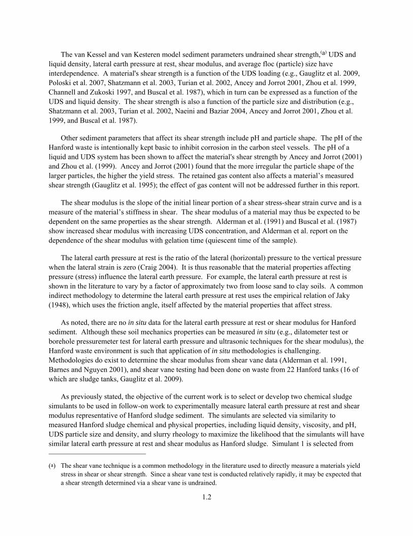
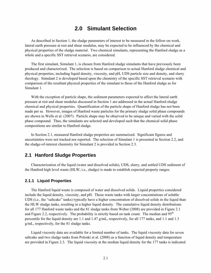
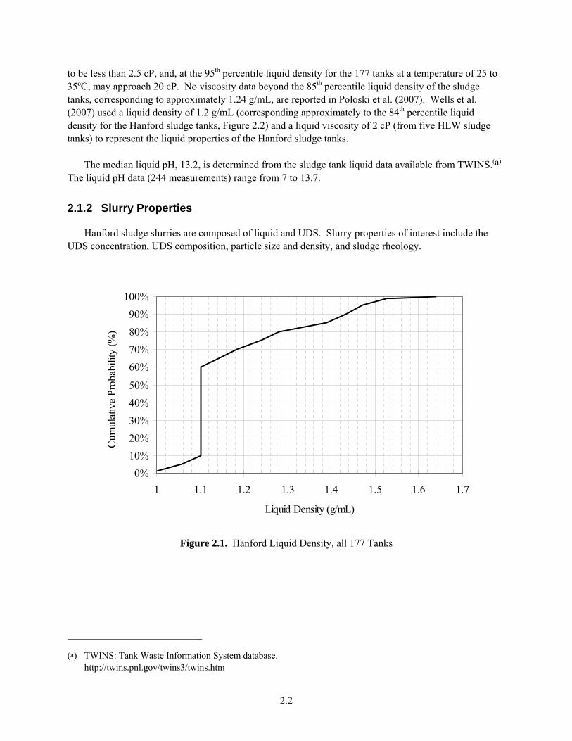
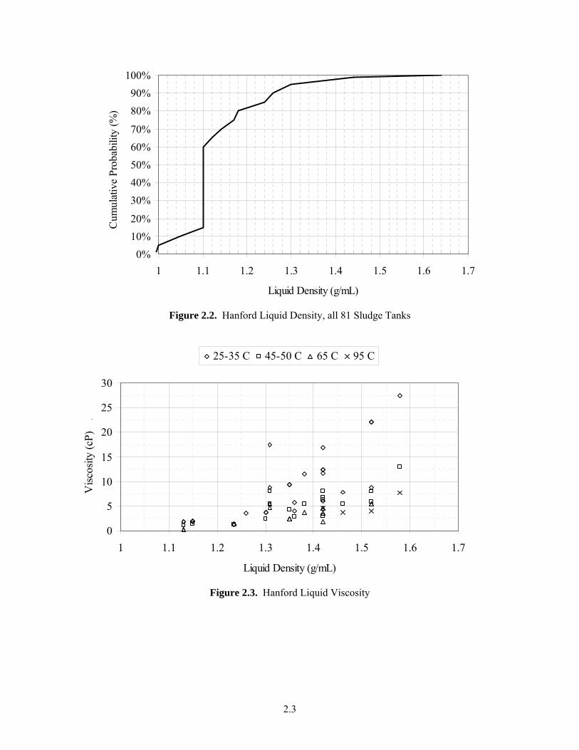
The Hanford liquid waste is composed of water and dissolved solids. Liquid properties considered include the liquid density, viscosity, and pH. Those waste tanks with larger concentrations of soluble UDS (i.e., the “saltcake” tanks) typically have a higher concentration of dissolved solids in the liquid than the HLW sludge tanks, resulting in a higher liquid density. The cumulative liquid density distributions for all 177 Hanford waste tanks and the 81 sludge tanks from Weber (2008) are provided in Figure 2.1 and Figure 2.2, respectively. The probability is strictly based on tank count. The median and 95th percentile for the liquid density are 1.1 and 1.47 g/mL, respectively, for all 177 tanks, and 1.1 and 1.3 g/mL, respectively, for the 81 sludge tanks.
Liquid viscosity data are available for a limited number of tanks. The liquid viscosity data for seven saltcake and two sludge tanks from Poloski et al. (2008) as a function of liquid density and temperature are provided in Figure 2.3. The liquid viscosity at the median liquid density for the 177 tanks is indicated
2.2
to be less than 2.5 cP, and, at the 95th percentile liquid density for the 177 tanks at a temperature of 25 to 35ºC, may approach 20 cP. No viscosity data beyond the 85th percentile liquid density of the sludge tanks, corresponding to approximately 1.24 g/mL, are reported in Poloski et al. (2007). Wells et al. (2007) used a liquid density of 1.2 g/mL (corresponding approximately to the 84th percentile liquid density for the Hanford sludge tanks, Figure 2.2) and a liquid viscosity of 2 cP (from five HLW sludge tanks) to represent the liquid properties of the Hanford sludge tanks.
The median liquid pH, 13.2, is determined from the sludge tank liquid data available from TWINS.(a) The liquid pH data (244 measurements) range from 7 to 13.7.
2.1.2 Slurry Properties
Hanford sludge slurries are composed of liquid and UDS. Slurry properties of interest include the UDS concentration, UDS composition, particle size and density, and sludge rheology.
0%
10%
20%
30%
40%
50%
60%
70%
80%
90%
100%
1 1.1 1.2 1.3 1.4 1.5 1.6 1.7
Liquid Density (g/mL)
Cum
ulat
ive
Pro
babi
lity
(%)
Figure 2.1. Hanford Liquid Density, all 177 Tanks
(a) TWINS: Tank Waste Information System database. http://twins.pnl.gov/twins3/twins.htm
2.3
0%
10%
20%
30%
40%
50%
60%
70%
80%
90%
100%
1 1.1 1.2 1.3 1.4 1.5 1.6 1.7
Liquid Density (g/mL)
Cum
ulat
ive
Pro
babi
lity
(%)
Figure 2.2. Hanford Liquid Density, all 81 Sludge Tanks
0
5
10
15
20
25
30
1 1.1 1.2 1.3 1.4 1.5 1.6 1.7
Liquid Density (g/mL)
Vis
cosi
ty (
cP)
.
25-35 C 45-50 C 65 C 95 C
Figure 2.3. Hanford Liquid Viscosity
2.4
2.1.2.1 Slurry UDS Concentration
The UDS concentration in settled sludge sediment may be expressed on a volume basis, and can be determined from
LS
LBS
(2.1)
where B is the bulk sediment density, S is the UDS density, and L is the liquid density. The UDS mass fraction can be computed from the volume fraction as
B
SSSw
(2.2)
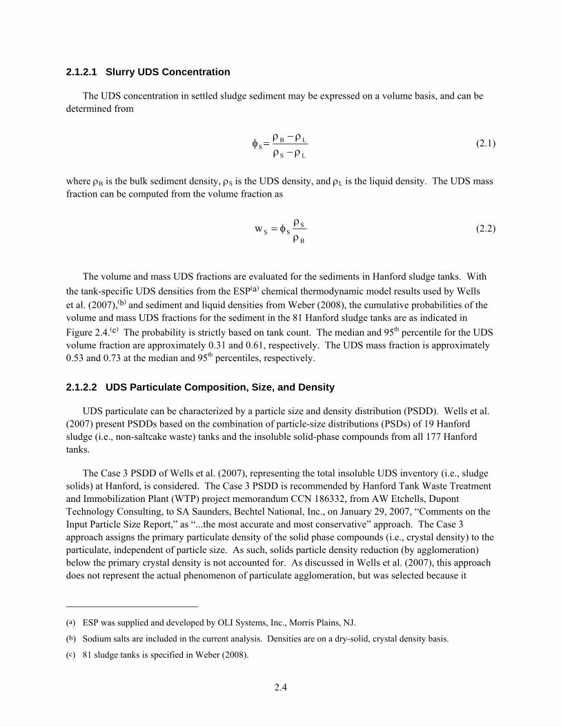
The volume and mass UDS fractions are evaluated for the sediments in Hanford sludge tanks. With
the tank-specific UDS densities from the ESP(a) chemical thermodynamic model results used by Wells et al. (2007),(b) and sediment and liquid densities from Weber (2008), the cumulative probabilities of the volume and mass UDS fractions for the sediment in the 81 Hanford sludge tanks are as indicated in
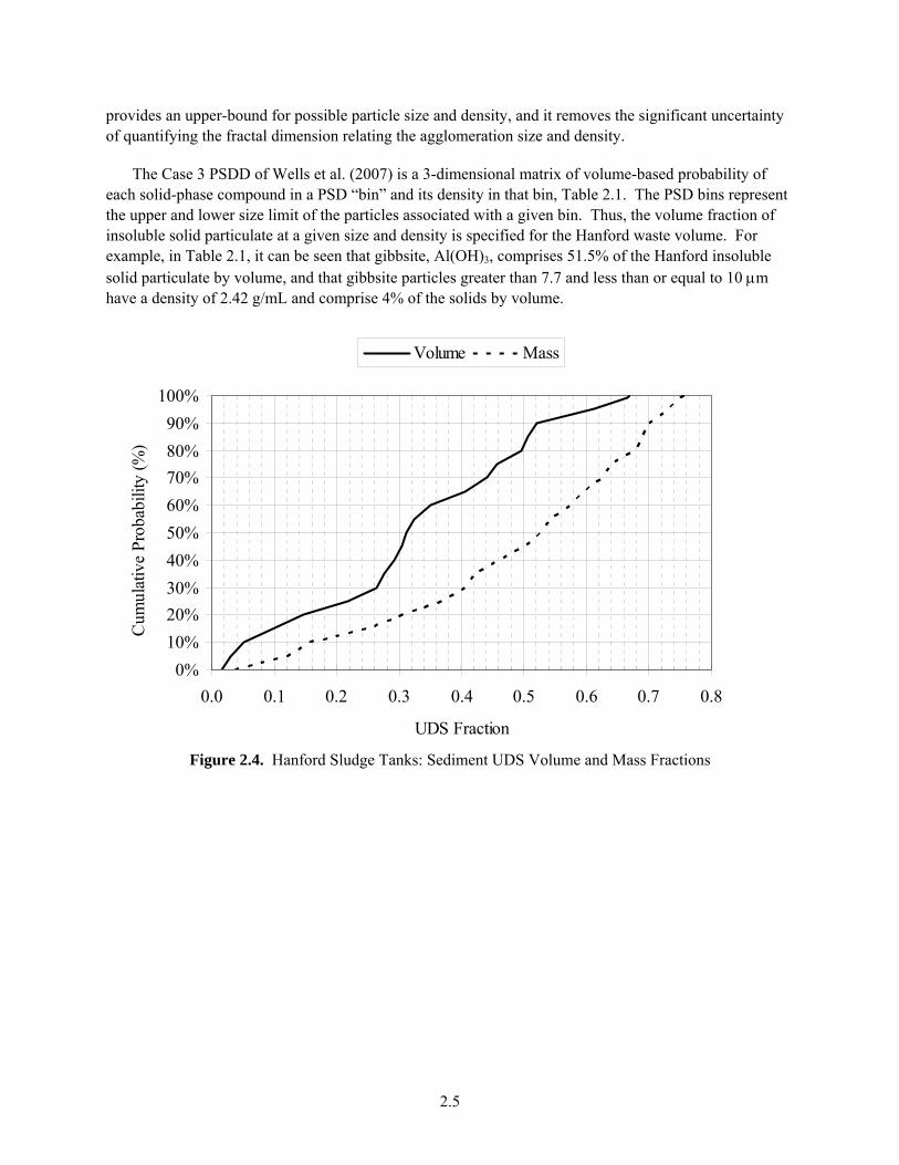
Figure 2.4.(c) The probability is strictly based on tank count. The median and 95th percentile for the UDS volume fraction are approximately 0.31 and 0.61, respectively. The UDS mass fraction is approximately 0.53 and 0.73 at the median and 95th percentiles, respectively.
2.1.2.2 UDS Particulate Composition, Size, and Density
UDS particulate can be characterized by a particle size and density distribution (PSDD). Wells et al. (2007) present PSDDs based on the combination of particle-size distributions (PSDs) of 19 Hanford sludge (i.e., non-saltcake waste) tanks and the insoluble solid-phase compounds from all 177 Hanford tanks.
The Case 3 PSDD of Wells et al. (2007), representing the total insoluble UDS inventory (i.e., sludge solids) at Hanford, is considered. The Case 3 PSDD is recommended by Hanford Tank Waste Treatment and Immobilization Plant (WTP) project memorandum CCN 186332, from AW Etchells, Dupont Technology Consulting, to SA Saunders, Bechtel National, Inc., on January 29, 2007, “Comments on the Input Particle Size Report,” as “...the most accurate and most conservative” approach. The Case 3 approach assigns the primary particulate density of the solid phase compounds (i.e., crystal density) to the particulate, independent of particle size. As such, solids particle density reduction (by agglomeration) below the primary crystal density is not accounted for. As discussed in Wells et al. (2007), this approach does not represent the actual phenomenon of particulate agglomeration, but was selected because it
(a) ESP was supplied and developed by OLI Systems, Inc., Morris Plains, NJ.
(b) Sodium salts are included in the current analysis. Densities are on a dry-solid, crystal density basis.
(c) 81 sludge tanks is specified in Weber (2008).
2.5
provides an upper-bound for possible particle size and density, and it removes the significant uncertainty of quantifying the fractal dimension relating the agglomeration size and density.
The Case 3 PSDD of Wells et al. (2007) is a 3-dimensional matrix of volume-based probability of each solid-phase compound in a PSD “bin” and its density in that bin, Table 2.1. The PSD bins represent the upper and lower size limit of the particles associated with a given bin. Thus, the volume fraction of insoluble solid particulate at a given size and density is specified for the Hanford waste volume. For example, in Table 2.1, it can be seen that gibbsite, Al(OH)3, comprises 51.5% of the Hanford insoluble solid particulate by volume, and that gibbsite particles greater than 7.7 and less than or equal to 10 m have a density of 2.42 g/mL and comprise 4% of the solids by volume.
0%
10%
20%
30%
40%
50%
60%
70%
80%
90%
100%
0.0 0.1 0.2 0.3 0.4 0.5 0.6 0.7 0.8
UDS Fraction
Cum
ulat
ive
Pro
babi
lity
(%)
Volume Mass
Figure 2.4. Hanford Sludge Tanks: Sediment UDS Volume and Mass Fractions

2.6
Table 2.1. Case 3 PSDD (Wells et al. 2007)
Particle Size (m)
Solid-Phase Compounds and Density (g/mL)
Total Volume Fraction
Al(OH)3
(NaAlSiO4)6• (NaNO3)1.6•
2H2O AlOOH NaAlCO3
(OH)2 Fe2O3 Ca5OH (PO4)3 Na2U2O7 ZrO2 Bi2O3 SiO2 Ni(OH)2 MnO2 CaF2
LaPO4• 2H2O Ag2CO3 PuO2
2.42 2.365 3.01 2.42 5.24 3.14 5.617 5.68 8.9 2.6 4.1 5.026 3.18 6.51 6.077 11.43
Solid Volume Fraction 0.22 1E-04 5E-05 3E-05 3E-05 1E-05 6E-06 5E-06 3E-06 2E-06 2E-06 2E-06 2E-06 7E-07 4E-07 3E-08 4E-09 2E-04 0.28 3E-04 1E-04 6E-05 6E-05 2E-05 1E-05 9E-06 6E-06 5E-06 4E-06 3E-06 3E-06 1E-06 8E-07 5E-08 8E-09 6E-04 0.36 6E-04 2E-04 1E-04 1E-04 5E-05 2E-05 2E-05 1E-05 1E-05 8E-06 7E-06 7E-06 3E-06 2E-06 1E-07 2E-08 1E-03 0.46 5E-05 2E-05 1E-05 1E-05 4E-06 2E-06 2E-06 1E-06 9E-07 7E-07 6E-07 6E-07 2E-07 1E-07 1E-08 1E-09 1E-04 0.60 2E-03 5E-04 3E-04 3E-04 1E-04 6E-05 5E-05 3E-05 2E-05 2E-05 2E-05 2E-05 7E-06 4E-06 3E-07 4E-08 3E-03 0.77 8E-03 3E-03 2E-03 1E-03 6E-04 3E-04 2E-04 2E-04 1E-04 1E-04 8E-05 8E-05 3E-05 2E-05 1E-06 2E-07 2E-02 1.0 2E-02 5E-03 3E-03 3E-03 1E-03 6E-04 5E-04 3E-04 2E-04 2E-04 2E-04 2E-04 7E-05 4E-05 3E-06 4E-07 3E-02 1.3 2E-02 6E-03 4E-03 4E-03 2E-03 8E-04 6E-04 4E-04 3E-04 3E-04 2E-04 2E-04 9E-05 5E-05 4E-06 5E-07 4E-02 1.7 3E-02 1E-02 7E-03 6E-03 3E-03 1E-03 1E-03 7E-04 5E-04 4E-04 4E-04 3E-04 1E-04 8E-05 6E-06 8E-07 6E-02 2.2 1E-02 5E-03 3E-03 3E-03 1E-03 5E-04 4E-04 3E-04 2E-04 2E-04 1E-04 1E-04 6E-05 4E-05 3E-06 4E-07 2E-02 2.8 4E-02 1E-02 7E-03 6E-03 3E-03 1E-03 1E-03 7E-04 6E-04 5E-04 4E-04 4E-04 2E-04 9E-05 6E-06 9E-07 7E-02 3.6 5E-02 2E-02 1E-02 9E-03 4E-03 2E-03 1E-03 1E-03 7E-04 6E-04 5E-04 5E-04 2E-04 1E-04 9E-06 1E-06 1E-01 4.6 3E-02 1E-02 6E-03 6E-03 3E-03 1E-03 1E-03 7E-04 5E-04 4E-04 3E-04 3E-04 1E-04 8E-05 6E-06 8E-07 6E-02 6.0 4E-02 1E-02 9E-03 8E-03 3E-03 2E-03 1E-03 9E-04 7E-04 6E-04 5E-04 4E-04 2E-04 1E-04 8E-06 1E-06 8E-02 7.7 5E-02 2E-02 1E-02 9E-03 4E-03 2E-03 2E-03 1E-03 8E-04 7E-04 5E-04 5E-04 2E-04 1E-04 9E-06 1E-06 1E-01 10 4E-02 1E-02 8E-03 7E-03 3E-03 2E-03 1E-03 9E-04 6E-04 5E-04 4E-04 4E-04 2E-04 1E-04 7E-06 1E-06 7E-02 13 4E-02 1E-02 8E-03 7E-03 3E-03 1E-03 1E-03 8E-04 6E-04 5E-04 4E-04 4E-04 2E-04 9E-05 7E-06 9E-07 7E-02 17 4E-02 1E-02 8E-03 7E-03 3E-03 2E-03 1E-03 8E-04 6E-04 5E-04 4E-04 4E-04 2E-04 1E-04 7E-06 1E-06 7E-02 22 3E-02 1E-02 6E-03 6E-03 2E-03 1E-03 9E-04 6E-04 5E-04 4E-04 3E-04 3E-04 1E-04 8E-05 5E-06 8E-07 6E-02 28 1E-02 5E-03 3E-03 3E-03 1E-03 6E-04 4E-04 3E-04 2E-04 2E-04 2E-04 2E-04 6E-05 4E-05 3E-06 4E-07 2E-02 36 2E-02 6E-03 4E-03 4E-03 2E-03 8E-04 6E-04 4E-04 3E-04 3E-04 2E-04 2E-04 9E-05 5E-05 4E-06 5E-07 4E-02 46 7E-03 2E-03 1E-03 1E-03 6E-04 3E-04 2E-04 1E-04 1E-04 9E-05 7E-05 7E-05 3E-05 2E-05 1E-06 2E-07 1E-02 60 5E-03 1E-03 9E-04 8E-04 4E-04 2E-04 1E-04 1E-04 7E-05 6E-05 5E-05 5E-05 2E-05 1E-05 8E-07 1E-07 9E-03 77 4E-03 1E-03 9E-04 8E-04 3E-04 2E-04 1E-04 9E-05 7E-05 6E-05 5E-05 4E-05 2E-05 1E-05 8E-07 1E-07 8E-03 100 3E-03 9E-04 5E-04 5E-04 2E-04 1E-04 8E-05 6E-05 4E-05 4E-05 3E-05 3E-05 1E-05 7E-06 5E-07 7E-08 5E-03 129 2E-03 6E-04 4E-04 3E-04 1E-04 7E-05 5E-05 4E-05 3E-05 2E-05 2E-05 2E-05 8E-06 4E-06 3E-07 4E-08 4E-03 167 7E-03 2E-03 1E-03 1E-03 5E-04 3E-04 2E-04 1E-04 1E-04 9E-05 7E-05 7E-05 3E-05 2E-05 1E-06 2E-07 1E-02 215 4E-03 1E-03 7E-04 7E-04 3E-04 1E-04 1E-04 8E-05 6E-05 5E-05 4E-05 4E-05 2E-05 9E-06 7E-07 9E-08 7E-03 278 2E-03 7E-04 4E-04 4E-04 2E-04 8E-05 6E-05 4E-05 3E-05 3E-05 2E-05 2E-05 9E-06 5E-06 4E-07 5E-08 4E-03 359 3E-03 1E-03 6E-04 5E-04 2E-04 1E-04 9E-05 6E-05 5E-05 4E-05 3E-05 3E-05 1E-05 7E-06 5E-07 8E-08 6E-03 464 6E-04 2E-04 1E-04 1E-04 5E-05 2E-05 2E-05 1E-05 1E-05 9E-06 7E-06 7E-06 3E-06 2E-06 1E-07 2E-08 1E-03 599 4E-04 1E-04 8E-05 7E-05 3E-05 1E-05 1E-05 8E-06 6E-06 5E-06 4E-06 4E-06 2E-06 1E-06 7E-08 1E-08 7E-04 774 4E-04 1E-04 9E-05 8E-05 3E-05 2E-05 1E-05 9E-06 7E-06 6E-06 4E-06 4E-06 2E-06 1E-06 8E-08 1E-08 8E-04 1000 3E-05 9E-06 6E-06 5E-06 2E-06 1E-06 8E-07 6E-07 4E-07 4E-07 3E-07 3E-07 1E-07 7E-08 5E-09 7E-10 6E-05
Total Volume Fraction
0.515 0.166 0.106 0.095 0.041 0.02 0.016 0.011 0.0081 0.0069 0.0055 0.0054 0.0023 0.0013 0.000094 0.000013 1.0
2.7
2.1.2.3 Rheology
Rheology data are available for a limited number of sludge tanks. Bingham model parameters for slurries and sediment shear strength are considered.
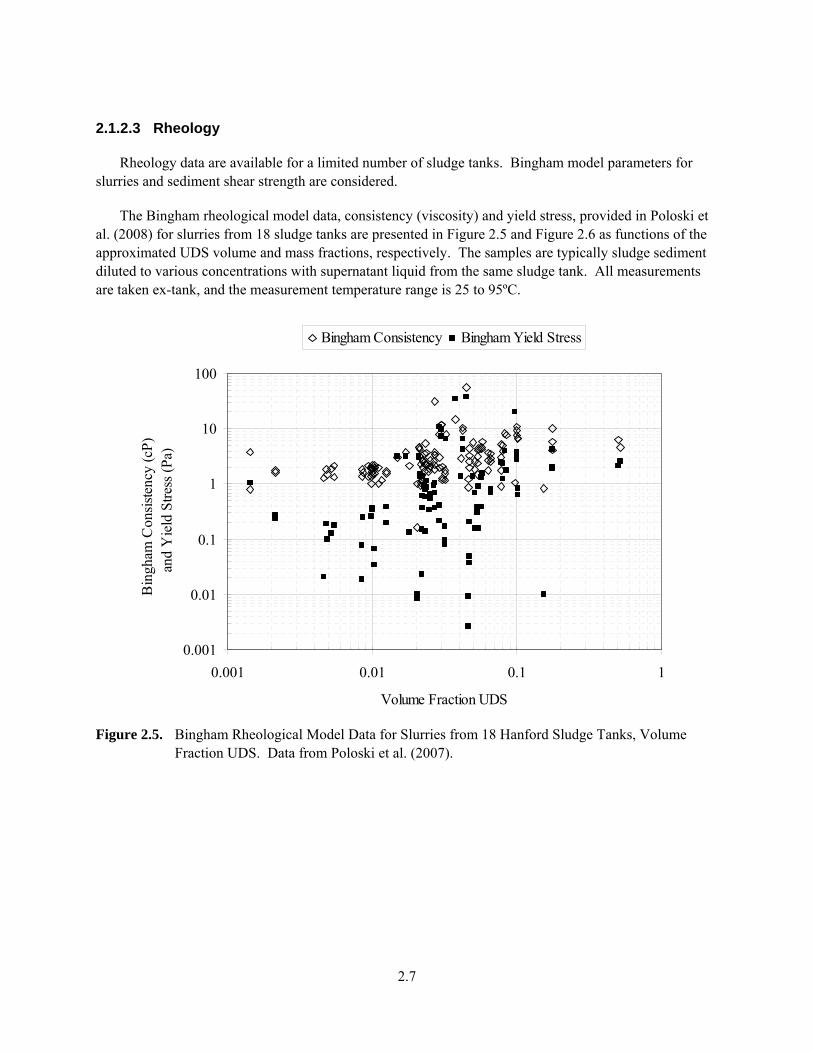
The Bingham rheological model data, consistency (viscosity) and yield stress, provided in Poloski et al. (2008) for slurries from 18 sludge tanks are presented in Figure 2.5 and Figure 2.6 as functions of the approximated UDS volume and mass fractions, respectively. The samples are typically sludge sediment diluted to various concentrations with supernatant liquid from the same sludge tank. All measurements are taken ex-tank, and the measurement temperature range is 25 to 95ºC.
0.001
0.01
0.1
1
10
100
0.001 0.01 0.1 1
Volume Fraction UDS
Bin
gham
Con
sist
ency
(cP
)
and
Yie
ld S
tres
s (P
a)
Bingham Consistency Bingham Yield Stress
Figure 2.5. Bingham Rheological Model Data for Slurries from 18 Hanford Sludge Tanks, Volume Fraction UDS. Data from Poloski et al. (2007).

2.8
0.001
0.01
0.1
1
10
100
0.001 0.01 0.1 1
Mass Fraction UDS
Bin
gham
Con
sist
ency
(cP
)
and
Yie
ld S
tres
s (P
a)
Bingham Consistency Bingham Yield Stress
Figure 2.6. Bingham Rheological Model Data for Slurries from 18 Hanford Sludge Tanks, Mass Fraction UDS. Data from Poloski et al. (2007).
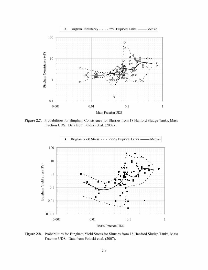
A 95% empirical limit for the Bingham rheological model data of Figure 2.6 is provided for the consistency and yield stress in Figure 2.7 and Figure 2.8. Partitions in the UDS mass fraction are taken, and the 2.5%, 50% (median), and 97.5 % probabilities of the partitions are determined. The resultant 95% empirical limit and median are represented in Figure 2.7 and Figure 2.8 at the average mass fraction UDS of the partitions. The lack of clear functionality of the Bingham model parameters with the UDS concentration may be expected because of the varied waste and sample conditions represented. The general expected trend (see references listed in Section 1) of increased rheology with increased UDS concentration is observable for the medians.
2.9
0.1
1
10
100
0.001 0.01 0.1 1
Mass Fraction UDS
Bin
gham
Con
sist
ency
(cP
)
Bingham Consistency 95% Empirical Limits Median
Figure 2.7. Probabilities for Bingham Consistency for Slurries from 18 Hanford Sludge Tanks, Mass Fraction UDS. Data from Poloski et al. (2007).
0.001
0.01
0.1
1
10
100
0.001 0.01 0.1 1
Mass Fraction UDS
Bin
gham
Yie
ld S
tres
s (P
a)
Bingham Yield Stress 95% Empirical Limits Median
Figure 2.8. Probabilities for Bingham Yield Stress for Slurries from 18 Hanford Sludge Tanks, Mass Fraction UDS. Data from Poloski et al. (2007).
2.10
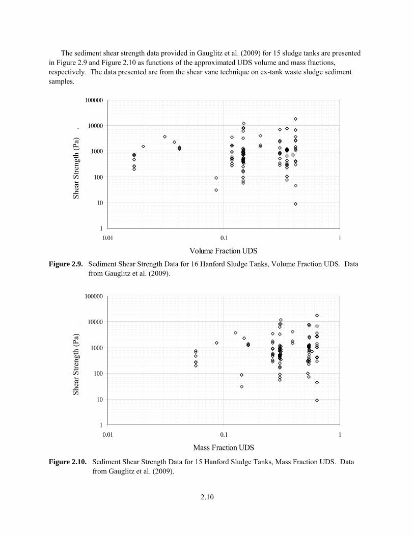
The sediment shear strength data provided in Gauglitz et al. (2009) for 15 sludge tanks are presented in Figure 2.9 and Figure 2.10 as functions of the approximated UDS volume and mass fractions, respectively. The data presented are from the shear vane technique on ex-tank waste sludge sediment samples.
1
10
100
1000
10000
100000
0.01 0.1 1
Volume Fraction UDS
She
ar S
tren
gth
(Pa)
.
Figure 2.9. Sediment Shear Strength Data for 16 Hanford Sludge Tanks, Volume Fraction UDS. Data from Gauglitz et al. (2009).
1
10
100
1000
10000
100000
0.01 0.1 1
Mass Fraction UDS
She
ar S
tren
gth
(Pa)
.
Figure 2.10. Sediment Shear Strength Data for 15 Hanford Sludge Tanks, Mass Fraction UDS. Data from Gauglitz et al. (2009).
2.11
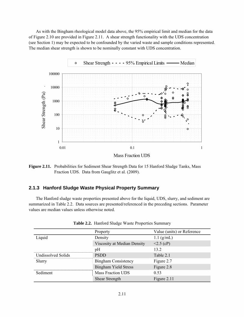
As with the Bingham rheological model data above, the 95% empirical limit and median for the data of Figure 2.10 are provided in Figure 2.11. A shear strength functionality with the UDS concentration (see Section 1) may be expected to be confounded by the varied waste and sample conditions represented. The median shear strength is shown to be nominally constant with UDS concentration.
1
10
100
1000
10000
100000
0.01 0.1 1
Mass Fraction UDS
She
ar S
tren
gth
(Pa)
.
Shear Strength 95% Empirical Limits Median
Figure 2.11. Probabilities for Sediment Shear Strength Data for 15 Hanford Sludge Tanks, Mass Fraction UDS. Data from Gauglitz et al. (2009).
2.1.3 Hanford Sludge Waste Physical Property Summary
The Hanford sludge waste properties presented above for the liquid, UDS, slurry, and sediment are summarized in Table 2.2. Data sources are presented/referenced in the preceding sections. Parameter values are median values unless otherwise noted.
Table 2.2. Hanford Sludge Waste Properties Summary
Property Value (units) or Reference Liquid Density 1.1 (g/mL)
Viscosity at Median Density <2.5 (cP) pH 13.2
Undissolved Solids PSDD Table 2.1 Slurry Bingham Consistency Figure 2.7
Bingham Yield Stress Figure 2.8 Sediment Mass Fraction UDS 0.53
Shear Strength Figure 2.11
2.12
2.2 Simulant 1 Selection
Simulants previously produced by Pacific Northwest National Laboratory (PNNL) with a level of complete characterization (some simulants were intended only as chemical simulants; therefore, rheology was not measured, etc.) include pretreated waste simulants AZ-101 (Stewart et al. 2007), AZ-101 (Golcar et al. 2000), AY-102 (Zamecnik et al. 2004), AZ-102 (Hansen et al. 2001), and the WTP crossflow ultrafiltration blended matrix simulant three (CBM-3) (Russell et al. 2009a).
The UDS portion of the AZ-101 of Stewart et al. (2007), AY-102, and AZ-102 referenced simulants was produced primarily by hydroxide precipitation (see Section 3). The hydroxide precipitation methodology is representative of the processes of UDS and supernate formation in the HLW tanks. The UDS of the AZ-101 simulant of Golcar et al. (2000) was provided via dry-powder solid-phase compounds, and the CBM-3 simulant was produced using a combination of the approaches. The CBM-3 simulant differs from the Pretreatment Engineering Platform (PEP) simulant (Kurath et al. 2009, Scheele et al. 2009) solely in minor trace metals of the precipitated hydroxide portion of the simulant. Subsequently, some of the reported characterizations for CBM-3 are taken from characterizations of the PEP simulant.
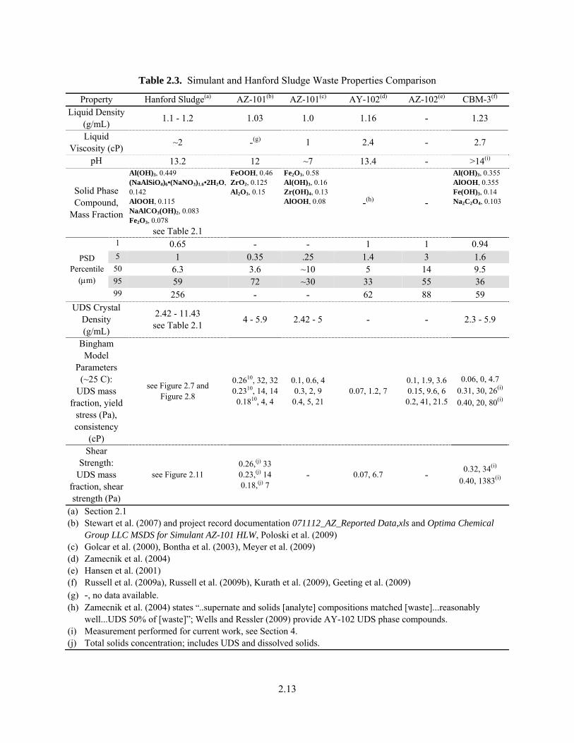
CBM-3 is selected as Simulant 1 because of its level of characterization and favorable comparison to Hanford sludge. A tabular comparison of the properties of the listed simulants to those of Hanford sludge is provided in Table 2.3. The AZ-102 simulant is discarded from further consideration as its characterization is incomplete relative to the other simulants. The AY-102 simulant also has a reduced level of characterization and is not considered further as those characterizations made are not substantively more comparative to Hanford sludge than those of the remaining three simulants. The AZ-101 simulant of Golcar et al. (2000) has its UDS fraction, as specified above, composed entirely of dry-powder solid-phase compounds. The UDS is composed primarily of an iron compound, while the Hanford sludge as a whole is predominantly aluminum. Further, its liquid phase is water, so the supernate density, viscosity, and pH are dissimilar to Hanford waste, and this simulant is thus not considered further.
The two remaining simulants for consideration include the precipitated hydroxide AZ-101 simulant (Stewart et al. 2007) and the CBM-3 simulant, which uses a combination of precipitated hydroxide and solid-phase compound powders. The liquid phase and predominant UDS phase compound of the Stewart et al. AZ-101 simulant are similar to the Golcar et al. AZ-101 simulant and do not represent the aggregate Hanford sludge as well as CBM-3.
2.13
Table 2.3. Simulant and Hanford Sludge Waste Properties Comparison
Property Hanford Sludge(a) AZ-101(b) AZ-101(c) AY-102(d) AZ-102(e) CBM-3(f) Liquid Density
(g/mL) 1.1 - 1.2 1.03 1.0 1.16 - 1.23
Liquid Viscosity (cP)
~2 -(g) 1 2.4 - 2.7
pH 13.2 12 ~7 13.4 - >14(i)
Solid Phase Compound,
Mass Fraction
Al(OH)3, 0.449 (NaAlSiO4)6•(NaNO3)1.6•2H2O, 0.142 AlOOH, 0.115 NaAlCO3(OH)2, 0.083 Fe2O3, 0.078
see Table 2.1
FeOOH, 0.46 ZrO2, 0.125 Al2O3, 0.15
Fe2O3, 0.58 Al(OH)3, 0.16 Zr(OH)4, 0.13 AlOOH, 0.08 -(h) -
Al(OH)3, 0.355 AlOOH, 0.355 Fe(OH)3, 0.14 Na2C2O4, 0.103
PSD Percentile
(m)
1 0.65 - - 1 1 0.94 5 1 0.35 .25 1.4 3 1.6 50 6.3 3.6 ~10 5 14 9.5 95 59 72 ~30 33 55 36 99 256 - - 62 88 59
UDS Crystal Density (g/mL)
2.42 - 11.43 see Table 2.1
4 - 5.9 2.42 - 5 - - 2.3 - 5.9
Bingham Model
Parameters (~25 C):
UDS mass fraction, yield
stress (Pa), consistency
(cP)
see Figure 2.7 and Figure 2.8
0.2610, 32, 32 0.2310, 14, 14 0.1810, 4, 4
0.1, 0.6, 4 0.3, 2, 9
0.4, 5, 21 0.07, 1.2, 7
0.1, 1.9, 3.6 0.15, 9.6, 6 0.2, 41, 21.5
0.06, 0, 4.7 0.31, 30, 26(i)
0.40, 20, 80(i)
Shear Strength:
UDS mass fraction, shear strength (Pa)
see Figure 2.11 0.26,(j) 33 0.23,(j) 14 0.18,(j) 7
- 0.07, 6.7 - 0.32, 34(i)
0.40, 1383(i)
(a) Section 2.1 (b) Stewart et al. (2007) and project record documentation 071112_AZ_Reported Data,xls and Optima Chemical
Group LLC MSDS for Simulant AZ-101 HLW, Poloski et al. (2009) (c) Golcar et al. (2000), Bontha et al. (2003), Meyer et al. (2009) (d) Zamecnik et al. (2004) (e) Hansen et al. (2001) (f) Russell et al. (2009a), Russell et al. (2009b), Kurath et al. (2009), Geeting et al. (2009) (g) -, no data available. (h) Zamecnik et al. (2004) states “..supernate and solids [analyte] compositions matched [waste]...reasonably
well...UDS 50% of [waste]”; Wells and Ressler (2009) provide AY-102 UDS phase compounds. (i) Measurement performed for current work, see Section 4. (j) Total solids concentration; includes UDS and dissolved solids.

2.14
An interesting distinction of the precipitated hydroxide simulants and those using solid-phase compound powders is their gravity-settling behavior. For actual Hanford waste, laboratory experiments (summary provided in Poloski et al. 2007) and in situ data (Gauglitz et al. 2009) indicate rapid UDS settling. The rapid Hanford UDS gravity settling rate is more closely represented by those simulants with the entire or portion of the UDS component from dry-powder solid-phase compounds. The AZ-101 simulant of Golcar et al. (2000) was observed to settle from a well-mixed condition to a settled solids
layer of approximately 30% by volume in less than approximately 4 to 5 days.(a) Laboratory settling of the CBM-3 simulant from a well-mixed condition to a settled solids layer of approximately 30% by volume in less than 10 hours is documented in Russell et al. (2009b).
Conversely, those simulants in which the UDS component was produced primarily by hydroxide precipitation are essentially non-settling. Following mixing and a nominally 3-day shut-down period, the AZ-101 simulant of Stewart et al. (2007) at nominally 18 wt% total solids was observed to have approximately 1% clear liquid by volume. At higher solid concentrations, settling was reduced.(b)
It is important to note that there are differences in laboratory and in situ settling data for actual Hanford waste. Per Gauglitz et al. (2009), the laboratory settling data evaluated by Poloski et al. (2007) suggest that in situ settling in the Hanford tanks would require about 50 times as long to settle as the laboratory tests. In fact, both the laboratory and in situ data show, summarized approximately here, the volume percent of slurry in a vessel (i.e., the portion of the vessel with a UDS fraction) as opposed to UDS-free liquid, from a well-mixed initial state at 100%, reduces to approximately 30% in less than 24 hours. Gauglitz et al. (2009) noted this inconsistency by stating:
“Scaling behavior, including the role of vessel size, of the settling dynamics and the buildup of strength in the settled layer, with a particular emphasis on shorter settling times and strength increase with depth into a layer is not well quantified with existing data and analysis. The best current estimates are presented in this report, but these estimates have uncertainty. Accurate predictions of the settling behavior and strength formation are needed, so the mixing system is designed to prevent settled layers that will exceed remobilization capabilities. Tank-farm studies of full-scale settling have shown substantially faster settling than expected based on laboratory tests. This inconsistency needs to be understood.”
The settling behavior of the CBM-3 simulant is more representative of the actual waste behavior than the AZ-101 (Stewart et al. 2007) simulant. The liquid phase parameters, PSD, UDS parameters, and rheology of the CBM-3 simulant reasonably represent Hanford sludge (as defined in Section 2.1) in comparison to the other simulants listed in Table 2.3. Thus, the CBM-3 simulant is selected as Simulant 1. Specific comparison of the Simulant 1 parameters to the Hanford sludge is made in Section 4.
(a) Behavior noted in laboratory record book for Bontha et al. (2000). Following mixing, the test (nominally 10-foot simulant depth in a 12.75-foot-diameter vessel, approximately 18 wt% total solids loading) was left in a shut-down condition and unattended for approximately 4 to 5 days. The settled condition was observed at the end of this time period.
(b) Behavior noted in laboratory record book for Stewart et al. (2007). Simulant depth approximately 52 inches; test vessel 70-inch diameter.

2.15
2.3 Simulant 2 Selection: Sludge-of-Interest Chemistry
As of 2009, it is planned to retrieve wastes from Tanks 241-C-104, C-111, and C-112 and relocate them into Tank AN-101. The sludge of interest, from the point of view of gas retention, is therefore a mixture of the four wastes. The constitutive properties of the mixture, and hence the potential for gas retention and release, cannot be predicted a priori. For this reason, characterization tests are to be performed on Simulant 2, which is a chemical simulant of the four-tank waste mixture.
The following procedure was used to develop the four-tank simulant chemical composition:
1) Obtain the average composition of the waste in each of the four tanks from predictions made by the
Environmental Simulation Program (ESP)(a) chemical thermodynamic model. The predictions were based on Best Basis Inventory (BBI) data. These predicted compositions are expressed in terms of compounds, not analytes, and provide distinct solid-phase and liquid-phase compositions.
2) Add the four inventories together, using the model-predicted volume fractions of liquid and dry solid, compositions of solid and liquid, and densities of solid and liquid, and the BBI estimates of total volume.
3) Assume that when the four tanks’ wastes are mixed, there is no reaction leading to precipitation or dissolution so that the liquid- and solid-phase compositions are preserved.
4) Calculate the concentrations of significant analytes in the bulk mixture and use these as the basis for the recipe. The simulant is produced by adding hydroxide to a mixture of metal nitrates to precipitate hydroxides and oxyhydroxides and then adding a slurry of the sodium salts and adding other metals as powders.
More details of the simulant development procedure are given in the following subsections.
2.3.1 Use of ESP Model Predictions
The BBIs for all 177 tanks, as of May 2002, were used to provide whole-tank-average composition inputs to the ESP model, which uses thermodynamic data to calculate the liquid and solid phase compositions at equilibrium. This modeling effort (Cowley et al. 2003) was carried out to support the development of a tank-by-tank toxic source term for use in tank farm safety analyses.
The ESP predictions constitute the only phase composition information that was available for Tanks AN-101, C-104, C-111, and C-112. Because the contents of the four tanks have not been changed by retrieval or transfer since 2002, the 2002 BBI information and the ESP predictions based on it are considered an appropriate basis for Simulant 2.
This application of ESP had certain characteristics that should be noted:
(a) ESP was supplied and developed by OLI Systems, Inc., Morris Plains, New Jersey.
2.16
Compositions were calculated on a whole-tank basis as if all the different layers of waste had been mixed and allowed to come to equilibrium.
ESP is an equilibrium model and is not expected to predict the correct concentration of any compounds that have not yet come to equilibrium with an in-tank chemical environment different from those in which they formed (e.g., different temperature, pH, etc.).
In the ESP runs carried out for Cowley et al. (2003), certain compounds were excluded from precipitating to reflect kinetic limitations or sometimes to reduce computational time or avoid nonconvergence of the solution algorithm.
Because of computational time constraints, reduction oxidation (REDOX) equilibrium was not calculated on a tank-by-tank basis in the 2003 study; rather, expert judgment and generic-composition runs of ESP were used to fix the metal oxidation states in all tanks. Iron was fixed as Fe+3, manganese as Mn+2, chromium as Cr+3 or Cr+6, U as U+6, and so forth. Thus, the ESP predictions did not include compounds formed by metals in any other oxidation states.
Because the 2003 study was aimed at toxicity assessment, and because the toxicity of organic compounds was calculated outside of ESP, the only organic species used in ESP inputs were oxalate and acetate ions. The former represented all the low-solubility carbon, the latter all the soluble carbon. Other organic species, including complexants, do not appear in the ESP results.
The study assigned compounds to the trace analytes (including thorium, cadmium, copper, tin, and many others) without employing the ESP model; thus, these metals are not present in the ESP-predictions database.
Thermodynamic data were not available for all the compounds that could potentially form in the tank waste, which led to the omission of some compounds.
The ESP model, as used, predicted the normalized concentration of each compound in the waste. In other words, the model predicted the relative masses of different compounds and the relative volumes and masses of total liquid and total solid, but not the absolute masses or volumes in a tank. The absolute volume of the dry-solid phase in a tank was calculated for the present study by combining the ESP results with BBI volumes, using the following equation:
ESPS VV (2.3)
where VS is the dry-solid volume in the tank, ESP is the ESP-predicted dry-solid fraction, average of all waste in the tank, and V is the total waste volume in the tank as defined by the BBI.
The solid-phase volume calculated by the above equation contains some uncertainty because of uncertainty in the parameters and because the potential retained gas volume is not accounted for.
2.17
2.3.2 Combination of Inventories for the Four Tanks of Interest
The contents of the four tanks of interest were described by the 2002 BBI as
AN-101: 956 kL of supernatant with no solids. The BBI did not identify a waste type.
C-104: 980 kL of sludge. Aluminum-clad fuel waste from the PUREX process (waste types CWP1 and CWP2), unidentified sludge, organic wash waste from PUREX (OWW3), Zircaloy-clad fuel waste from the PUREX and Zirflex processes (CWZr1), and thorium fuel waste from PUREX (TH2) were listed as contributors, in decreasing order of volume.
C-111: 217 kL of sludge. Waste from ferrocyanide scavenging of supernatants (TFeCN), CWP1, waste from the BiPO4 fuel-recovery process (1C), and waste from the hot semiworks pilot plant (HS) were listed as contributors, in decreasing order of volume.
C-112: 393 kL of sludge. Waste types TFeCN, CWP1, and1C were listed as contributors, in decreasing order of volume.
The interstitial liquid composition was not given in the BBIs for any of the three C tanks. The ESP prediction was therefore taken as guidance to the liquid composition.
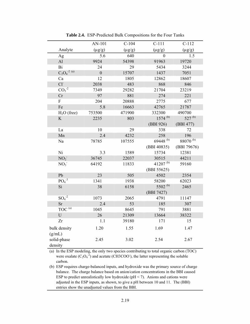
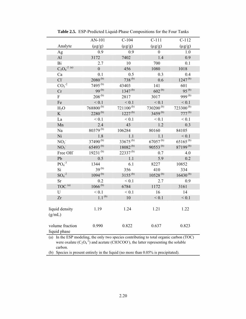
Table 2.4 gives the bulk compositions that were derived from ESP modeling results for the four tanks. Table 2.5 gives the liquid-phase compositions predicted by ESP and indicates which species were present only in liquid form.
As is shown in Table 2.4, the calculated bulk compositions for Tanks C-111 and C-112 differ from the average tank waste composition in the BBI. This is the result of intentional changes that were made to adapt the BBI average bulk concentrations to the input requirements of ESP. The ESP model requires charge-balanced composition input, and the charge balance of the unadjusted BBI bulk compositions for C-111 and C-112 led to an unreasonably low hydroxide concentration, giving a pH of less than 7. The BBI composition was therefore adjusted to contain higher cation concentrations (Na+ and K+), and, in the case of C-111, lower anion concentrations (NO3
- and SiO4-4). The adjustment allowed for higher
concentrations of free hydroxide, which made up the charge balance.
Another difference from the BBI can be seen in the solids predicted in AN-101. Only liquid was present in AN-101, according to the 2002 BBI. The ESP-predicted solids, which are 2.0 wt% of the inventory, include Al(OH)3 and small contributions from a range of compounds of other metals. The Al solubility implied by the dissolved Al concentration in the BBI was about triple the ESP prediction: 9914 g/g (0.44 M), rather than the predicted 3172 g/g (0.14 M).
It is not clear that the Al concentrations given in the BBI came from direct measurements that were made at the BBI’s free hydroxide concentration of 16838 g/g (1.18 M). The BBI was based partly on measurements made in 1998 and partly on additions of water and AX-farm liquid between 1998 and 2002. For comparison, two liquid grab samples taken in 1998 (1AN-98-2 and 1AN-98-3) contained 9430 to 9990 g/mL of Al (0.35 to 0.37 M) in combination with 26700 to 33100 g/mL of hydroxide (1.57 to 1.95 M). The measurements show that about the same concentration of Al as in the BBI was produced by a considerably higher hydroxide concentration. This suggests that the BBI calculations may have made assumptions that overestimated the concentration of Al that could be supported by the BBI-calculated
2.18
hydroxide concentration. On the other hand, the dissolved Al concentrations predicted by ESP seem low; the ratio of Al/free OH is less for the ESP predictions than for the grab samples.
The total liquid-phase and solid-phase masses in each tank were calculated by multiplying the BBI total volume by the liquid-phase and solid-phase volume fractions and densities calculated by ESP. The mass inventory of each ESP-predicted compound in each phase was then calculated by multiplying the phase mass by the ESP-predicted compound concentration in the phase. Finally, the analyte inventories in each phase were calculated from the inventories of compounds and summed over all four tanks.
No attempt was made to account for any dissolution or precipitation that might have resulted from mixing the wastes. Hence, the liquid-phase concentrations should not be considered to be specific predictions. Aluminum would be the likeliest candidate for a phase change that would lead to different phase concentrations than those given by a simple summation; fluoride and phosphate are other possibilities. Note, however, that the bulk composition, which is unaffected by precipitation and dissolution, is the information that is relevant to simulant development. As Section 3.2 shows, the simulant makeup process does not depend on the speciation or phase distribution predicted by ESP.
2.19
Table 2.4. ESP-Predicted Bulk Compositions for the Four Tanks
Analyte AN-101 (g/g)
C-104 (g/g)
C-111 (g/g)
C-112 (g/g)
Ag 5.6 640 0 1.5 Al 9924 54398 91963 19720 Bi 24 29 5434 3244 C2O4
-2 (a) 0 15707 1437 7051 Ca 12 1805 12862 18607 Cl- 2038 483 868 846 CO3
-2 7349 29282 21704 23219 Cr 97 881 274 221 F 204 20888 2775 677 Fe 5.8 16663 42765 21787 H2O (free) 753500 471900 332300 490700 K 2235 803 1574 (b)
(BBI 926) 527 (b)
(BBI 477) La 10 29 338 72 Mn 2.4 4232 258 196 Na 78785 107555 69448 (b)
(BBI 40835) 88070 (b)
(BBI 79676) Ni 3.3 1589 15734 12381 NO2
- 36745 22037 30515 44211 NO3
- 64192 11833 41207 (b)
(BBI 55625) 59160
Pb 23 505 4502 2354 PO4
-3 1341 1938 58200 62023 Si 38 6158 5502 (b)
(BBI 7427) 2465
SO4-2 1073 2065 4791 11147
Sr 2.4 53 185 307 TOC (a) 1045 8645 791 3881 U 26 21309 13664 38322 Zr 1.1 39180 171 15
bulk density (g/mL)
1.20 1.55 1.69 1.47
solid-phase density
2.45 3.02 2.54 2.67
(a) In the ESP modeling, the only two species contributing to total organic carbon (TOC) were oxalate (C2O4
-2) and acetate (CH3COO-), the latter representing the soluble carbon.
(b) ESP requires charge-balanced inputs, and hydroxide was the primary source of charge balance. The charge balance based on anion/cation concentrations in the BBI caused ESP to predict unrealistically low hydroxide (pH < 7). Anions and cations were adjusted in the ESP inputs, as shown, to give a pH between 10 and 11. The (BBI) entries show the unadjusted values from the BBI.
2.20
Table 2.5. ESP-Predicted Liquid-Phase Compositions for the Four Tanks
Analyte AN-101 (g/g)
C-104 (g/g)
C-111 (g/g)
C-112 (g/g)
Ag 0.9 0.9 0 1.0 Al 3172 7402 1.4 0.9 Bi 2.7 10 700 0.1 C2O4
-2 (a) 0 456 1080 1018 Ca 0.1 0.5 0.3 0.4 Cl- 2080 (b) 738 (b) 0.6 1247 (b) CO3
-2 7495 (b) 43403 141 601 Cr 99 (b) 1347 (b) 602 (b) 95 (b) F 208 (b) 2817 3017 999 (b) Fe < 0.1 < 0.1 < 0.1 < 0.1 H2O 768800 (b) 721100 (b) 730200 (b) 723300 (b) K 2280 (b) 1227 (b) 3459 (b) 777 (b) La < 0.1 < 0.1 < 0.1 < 0.1 Mn 2.4 43 1.2 0.3 Na 80379 (b) 106284 80160 84105 Ni 1.8 1.1 1.1 < 0.1 NO2
- 37490 (b) 33675 (b) 67057 (b) 65165 (b) NO3
- 65493 (b) 18082 (b) 90553 (b) 87199 (b) Free OH- 19231 (b) 22337 (b) 0.7 4.0 Pb 0.5 1.1 5.9 0.2 PO4
-3 1344 6.1 8227 10852 Si 39 (b) 356 410 334 SO4
-2 1094 (b) 3155 (b) 10528 (b) 16430 (b) Sr 0.2 < 0.1 2.7 0.9 TOC (a) 1066 (b) 6784 1172 3161 U < 0.1 < 0.1 16 14 Zr 1.1 (b) 10 < 0.1 < 0.1
liquid density (g/mL)
1.19 1.24 1.21 1.22
volume fraction liquid phase
0.990 0.822 0.637 0.823
(a) In the ESP modeling, the only two species contributing to total organic carbon (TOC) were oxalate (C2O4
-2) and acetate (CH3COO-), the latter representing the soluble carbon.
(b) Species is present entirely in the liquid (no more than 0.05% is precipitated).

2.21
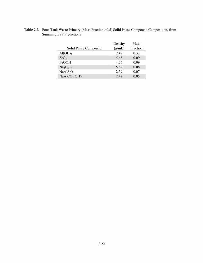
Table 2.6 shows the bulk and liquid-phase analyte concentrations that were calculated for the four-tank mixed waste. The predominant solid compound (more than 30 wt% of the solid phase) was calculated to be Al(OH)3, Table 2.7.
Table 2.6. Four-Tank Waste Mixture Composition, from Summing ESP Predictions
Analyte Concentration in Bulk
(g/g) Concentration in Liquid
(g/g) Ag 271 0.9 Al 38522 4080 Bi 1091 48 C2O4
-2 (a) 7881 386 Ca 5048 0.3 Cl- 1074 1330 CO3
-2 20571 19354 Cr 465 593 F 9240 1467 Fe 14839 < 0.1 H2O 550210 741989 (b) K 1292 1742 La 61 < 0.1 Mn 1838 17 Na 91422 90523 Ni 4249 1 NO2
- 31121 41969 (b) NO3
- 39031 52635 (b) Free OH- --- 16369 (b) Pb 1054 1 PO4
-3 17079 2669 Si 3555 223 SO4
-2 3480 4694 (b) Sr 91 0.4 TOC (a) 4670 3502 U 16494 3 Zr 16499 4
density (g/mL)
1.42 1.21
volume fraction --- 0.74 (a) In the ESP modeling, the only two species contributing to TOC were oxalate
(C2O4-2) and acetate (CH3COO-), the latter representing the soluble carbon.
(b) Species is present entirely in the liquid (no more than 0.05% is precipitated).
2.22
Table 2.7. Four-Tank Waste Primary (Mass Fraction >0.5) Solid Phase Compound Composition, from Summing ESP Predictions
Solid Phase Compound Density (g/mL)
Mass Fraction
Al(OH)3 2.42 0.33 ZrO2 5.68 0.09 FeOOH 4.26 0.09 Na2U2O7 5.62 0.08 NaAlSiO4 2.59 0.07 NaAlCO3(OH)2 2.42 0.05
3.1
3.0 Simulant Preparation
Specific preparation is documented for the two sludge simulants. The preparation of Simulant 1 is described in Section 3.1, and that of Simulant 2 in Section 3.2.
3.1 Simulant 1 Preparation
Previous work developed a simulant used in the WTP PEP ultra-filtration testing and is known as the CBM-3 simulant (Russell et al. 2009a). The CBM-3 simulant was selected as Simulant 1 for the current work as described in Section 2 and consists of a complex hydroxide precipitation methodology to produce the iron-bearing portion of the simulant, which is representative of the method by which this phase was formed in the HLW tanks, along with an anion-bearing supernate. Simulant 1 also contains a blend of commercially available materials, including sodium oxalate, boehmite, and gibbsite.
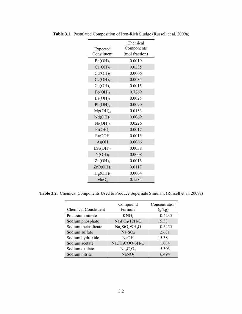
The iron-bearing portion of Simulant 1 represents the hydroxide waste phases that formed in the tank waste when metal nitrate solutions (mainly iron) were treated with caustic to minimize corrosion (Gephart and Lundgren 2005). The composition of this portion of the simulant was simplified by removing minor elements that were also toxic. No aging of the iron-bearing portion, such as the heat treatment performed by Stewart et al. (2007), was conducted. The iron-bearing portion of the simulant was based on the composition of the AY-102/C-106 tank waste sludge, minus the gibbsite, boehmite, chromium, and minor metals, and was prepared as described by Zamecnik et al. (2004), having the components listed in Table 3.1 and Table 3.2.
Table 3.1 shows the postulated UDS chemical components of the iron-bearing sludge portion of the simulant, which consists primarily of iron. The insoluble hydroxide solids are produced when NaOH is added to a metal nitrate solution, increasing the pH to between 10 and 11. The KMnO4 and Mn(NO3)2 are pre-reacted to produce insoluble MnO2 before the nitrate salts are added by mixing them together in deionized water. The excess nitrate is then washed from the slurry using the simple supernate described in Appendix A. Table 3.2 shows the chemical components used to produce the final supernate simulant and includes both the nitrate and non-nitrate anions present in the waste. The recipe used to make the iron-bearing and supernate simulant portions of Simulant 1 is provided as Appendix A.
Gibbsite, boehmite, and sodium oxalate were added to the iron-bearing and supernatant simulants. Sodium oxalate is included in the solids phase of the simulant for several reasons. It is one of the principal organic salts in the Hanford wastes. In general, oxalates have a low solubility and are temperature sensitive compared to other salts in the waste and oxalate complexes with ferric iron to form a soluble iron complex. In the simulant, it is used to also represent all of the minor water-soluble constituents of the solids phase such as the carbonates, sulfates, phosphates, oxalates, and fluoride-phosphates (Smith et al. 2009). The component masses to produce nominally 5 L of Simulant 1 at approximately 40 wt% UDS are provided in Appendix B. Also provided in Appendix B are the manufacturer characterizations of the primary solid-phase compounds gibbsite and boehmite.
3.2
Table 3.1. Postulated Composition of Iron-Rich Sludge (Russell et al. 2009a)
Expected Constituent
Chemical Components
(mol fraction)
Ba(OH)2 0.0019
Ca(OH)2 0.0235
Cd(OH)2 0.0006
Ce(OH)3 0.0034
Cu(OH)2 0.0015
Fe(OH)3 0.7269
La(OH)3 0.0025
Pb(OH)2 0.0090
Mg(OH)2 0.0153
Nd(OH)3 0.0069
Ni(OH)2 0.0226
Pr(OH)3 0.0017
RuOOH 0.0013
AgOH 0.0066
kSr(OH)2 0.0038
Y(OH)3 0.0008
Zn(OH)2 0.0013
ZrO(OH)2 0.0117
Hg(OH)2 0.0004
MnO2 0.1584
Table 3.2. Chemical Components Used to Produce Supernate Simulant (Russell et al. 2009a)
Chemical Constituent Compound
Formula Concentration
(g/kg)
Potassium nitrate KNO3 0.4235 Sodium phosphate Na3PO4•12H2O 15.38 Sodium metasilicate Na2SiO3•9H2O 0.5455 Sodium sulfate Na2SO4 2.671 Sodium hydroxide NaOH 15.38 Sodium acetate NaCH3COO•3H2O 1.034 Sodium oxalate Na2C2O4 5.303 Sodium nitrite NaNO2 6.494
3.3
3.2 Simulant 2 Preparation
Simulant 2, whose composition is based on the four-tank waste mixture described by Table 2.4, was produced via a four-step procedure:
1) Create a simulant of the sodium salts present in the four-tank mixed waste. This salt slurry is made up from water and sodium acetate, oxalate, chloride, carbonate, fluoride, nitrite, nitrate, phosphate, and sulfate. The recipe for this salt slurry is calculated from the bulk concentrations of TOC, C2O4
-2, Cl-, CO3
-2, F-, NO2-, NO3
-, PO4-3, and SO4
-2.
2) Add hydroxide to a mixture of acid nitrates of the metals Ni, Fe, Nd, Mn, and Ca. Neodymium is used as a surrogate for uranium. The recipe for this slurry of metal hydroxides and oxides is calculated from the bulk concentrations of Ni, Fe, U, Mn, and Ca. Manganese is added in the Mn(II) oxidation state.
3) Combine the slurries produced by Steps (1) and (2).
4) Add Al(OH)3, ZrO2, and SiO2 as powders; some portion of these powders is expected to dissolve as with Simulant 1. The amounts of powders added are based on the bulk concentrations of Al, Zr, and Si.
This approach was used to produce some of the solids in the same general manner in which they formed in the tanks through precipitation when hydroxide was added to a solution of nitrates. The recipe used to prepare Simulant 2 is provided as Appendix C. The component masses to produce nominally 15 L of Simulant 2 at approximately 23 wt% UDS are provided the Appendix as well.


4.1
4.0 Simulant Properties
Material properties for Simulants 1 and 2 are listed together with, where applicable, the comparative Hanford sludge properties. The material properties considered include the chemical composition, liquid density, viscosity, and pH, UDS particle size and density, and slurry rheology. The shear modulus of the simulants is estimated. Settling data are also presented, and particle images are shown. The influence of these properties on the lateral earth pressure at rest and shear modulus is discussed in Section 1. Unless otherwise referenced, Simulant 1 and Hanford sludge data are from Section 2, and Simulant 2 data are from the current analysis. Where pertinent, the instrumentation used to perform the measurements is listed together with the operational procedure. Significant figures and uncertainties were not tracked nor reported.
4.1 Chemical Composition
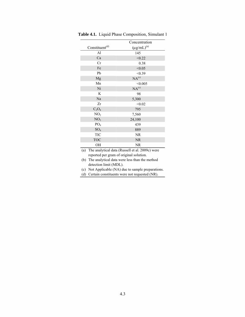
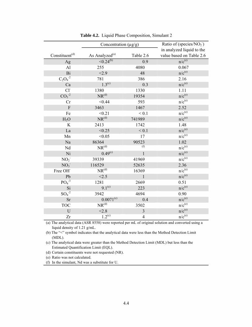
The analyte concentrations for the liquid phase of Simulants 1 and 2 are provided in Table 4.1 and Table 4.2, respectively. The Simulant 2 liquid composition for the SST retrieval scenario (Section 2.3, Table 2.6) is included for comparison. The slurry phase composition of Simulant 1 is provided in Table 4.3, and the slurry phase composition of Simulant 2 together with the SST retrieval scenario slurry composition (Section 2.3, Table 2.6) are provided in Table 4.4. The composition of Simulant 2 is shown to compare well with the SST retrieval scenario considered in Section 2.3.
Table 4.2 and Table 4.4 each contain a column that shows how each species concentration, when normalized using one of the other major constituents, compares to expectations. The normalization makes up for any variation caused by having more, or less, water present in the simulant than in the Table 2.6 compositions.
In the case of liquid-phase concentrations (Table 4.2), nitrite is used to normalize the other dissolved species. Nitrite is expected to be completely soluble. The dissolved concentrations of sodium, chloride, and sulfate all match the expectations within about 10%. The somewhat high potassium in the liquid (48% high) may have come from trace contamination of reagents with potassium. Oxalate, aluminum, fluoride, and phosphate all apparently have different solubilities than the Table 2.6 estimates (data included in Table 4.2), which were based on taking a weighted sum of the ESP-predicted dissolved concentrations for the four sludge tanks (giving the values in Table 2.6). This difference from the Table 2.6 results is not surprising since the solubility of a species in a mixture of liquids can be non-linearly different than the solubility in each liquid. Finally, the nitrate in the liquid is more than double the expected concentration. This is the result not of a solubility difference, but of unavoidable excess nitrate from the metal nitrates used as reagents to produce the simulant.
In the case of slurry concentrations (Table 4.4), iron is used to normalize the other species. Iron is expected to be effectively insoluble. The normalized concentrations of all the analyzed species in the simulant are within about 10% of the values based on Table 2.6 (data included in Table 4.4), except in the case of potassium. As already stated, the increase in potassium may have come from trace contaminants in the reagents.
4.2
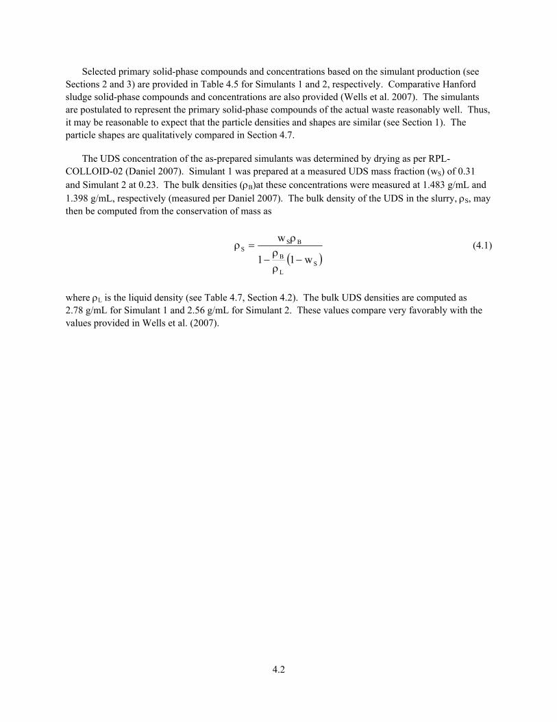
Selected primary solid-phase compounds and concentrations based on the simulant production (see Sections 2 and 3) are provided in Table 4.5 for Simulants 1 and 2, respectively. Comparative Hanford sludge solid-phase compounds and concentrations are also provided (Wells et al. 2007). The simulants are postulated to represent the primary solid-phase compounds of the actual waste reasonably well. Thus, it may be reasonable to expect that the particle densities and shapes are similar (see Section 1). The particle shapes are qualitatively compared in Section 4.7.
The UDS concentration of the as-prepared simulants was determined by drying as per RPL-COLLOID-02 (Daniel 2007). Simulant 1 was prepared at a measured UDS mass fraction (wS) of 0.31 and Simulant 2 at 0.23. The bulk densities (B)at these concentrations were measured at 1.483 g/mL and 1.398 g/mL, respectively (measured per Daniel 2007). The bulk density of the UDS in the slurry, S, may then be computed from the conservation of mass as
SL
B
BSS
w11
w
(4.1)
where L is the liquid density (see Table 4.7, Section 4.2). The bulk UDS densities are computed as 2.78 g/mL for Simulant 1 and 2.56 g/mL for Simulant 2. These values compare very favorably with the values provided in Wells et al. (2007).
4.3
Table 4.1. Liquid Phase Composition, Simulant 1
Constituent(d) Concentration
(g/mL)(a) Al 145 Ca <0.22 Cr 0.38 Fe <0.05 Pb <0.39
Mg NA(c) Mn <0.005 Ni NA(c) K 98
Na 5,300 Zr <0.02
C2O4 795 NO2 7,560 NO3 24,100 PO4 439 SO4 889 TIC NR
TOC NR OH NR
(a) The analytical data (Russell et al. 2009c) were reported per gram of original solution.
(b) The analytical data were less than the method detection limit (MDL).
(c) Not Applicable (NA) due to sample preparations.(d) Certain constituents were not requested (NR).
4.4
Table 4.2. Liquid Phase Composition, Simulant 2
Constituent(d)
Concentration (g/g) Ratio of (species/NO2-)
in analyzed liquid to the value based on Table 2.6 As Analyzed(a) Table 2.6
Ag <0.24(b) 0.9 n/c(e) Al 255 4080 0.067 Bi <2.9 48 n/c(e)
C2O4-2 781 386 2.16
Ca 1.3(c) 0.3 n/c(e) Cl- 1380 1330 1.11
CO3-2 NR(d) 19354 n/c(e)
Cr <0.44 593 n/c(e) F 3463 1467 2.52
Fe <0.21 < 0.1 n/c(e) H2O NR(d) 741989 n/c(e)
K 2413 1742 1.48 La <0.25 < 0.1 n/c(e)
Mn <0.05 17 n/c(e) Na 86364 90523 1.02 Nd NR(d) (f) n/c(e) Ni 0.49(c) 1 n/c(e)
NO2- 39339 41969 n/c(e)
NO3- 116529 52635 2.36
Free OH- NR(d) 16369 n/c(e) Pb <2.5 1 n/c(e)
PO4-3 1281 2669 0.51
Si 9.1(c) 223 n/c(e) SO4
-2 3942 4694 0.90 Sr 0.0071(c) 0.4 n/c(e)
TOC NR(d) 3502 n/c(e) U <2.8 3 n/c(e) Zr 1.2(c) 4 n/c(e)
(a) The analytical data (ASR 8558) were reported per mL of original solution and converted using a liquid density of 1.21 g/mL.
(b) The “<” symbol indicates that the analytical data were less than the Method Detection Limit (MDL).
(c) The analytical data were greater than the Method Detection Limit (MDL) but less than the Estimated Quantification Limit (EQL).
(d) Certain constituents were not requested (NR). (e) Ratio was not calculated. (f) In the simulant, Nd was a substitute for U.

4.5
Table 4.3. Slurry Phase Composition, Simulant 1
Constituent Concentration
(g/g)(a) Ag 107 Al 33,400 Ba 343(b) Ca <4660 Ce 61(b) Cd <12.3 Cr 136 Cu 43(b) Fe 6,900(b) K NA(c)
La 48(b) Mg 83(b) Mn 1,490 Na 304,000 Ni NA(c) Nd 120(b)
P 1,300(b) Pb 460(b) S 1,500(b)
Sr 54.3 Zn 56(b) Zr 61(b)
C2O4 NR(d) NO2 NR(d) NO3 NR(d) PO4 NR(d) SO4 NR(d) TIC NR(d)
TOC NR(d) OH NR(d)
(a) The analytical data are reported per gram of original slurry. Project records for Russell et al. (2009c).
(b) The analytical results are greater than the MDL but less than the estimated quantification limit (EQL).
(c) Not Applicable due to potassium hydroxide (KOH) fusion.
(d) Not Reported.
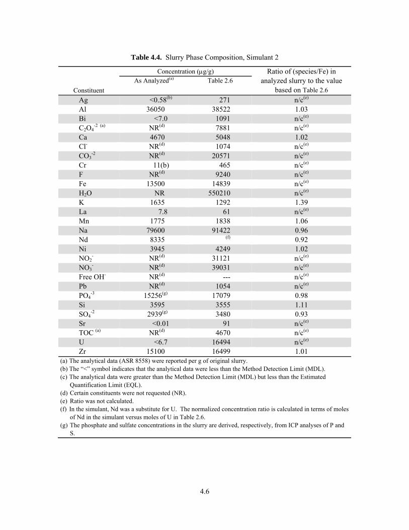
4.6
Table 4.4. Slurry Phase Composition, Simulant 2
Constituent
Concentration (g/g) Ratio of (species/Fe) in analyzed slurry to the value
based on Table 2.6
As Analyzed(a) Table 2.6
Ag <0.58(b) 271 n/c(e) Al 36050 38522 1.03 Bi <7.0 1091 n/c(e) C2O4
-2 (a) NR(d) 7881 n/c(e) Ca 4670 5048 1.02 Cl- NR(d) 1074 n/c(e) CO3
-2 NR(d) 20571 n/c(e) Cr 11(b) 465 n/c(e) F NR(d) 9240 n/c(e) Fe 13500 14839 n/c(e) H2O NR 550210 n/c(e) K 1635 1292 1.39 La 7.8 61 n/c(e) Mn 1775 1838 1.06 Na 79600 91422 0.96 Nd 8335 (f) 0.92 Ni 3945 4249 1.02 NO2
- NR(d) 31121 n/c(e) NO3
- NR(d) 39031 n/c(e) Free OH- NR(d) --- n/c(e) Pb NR(d) 1054 n/c(e) PO4
-3 15256(g) 17079 0.98 Si 3595 3555 1.11 SO4
-2 2939(g) 3480 0.93 Sr <0.01 91 n/c(e) TOC (a) NR(d) 4670 n/c(e) U <6.7 16494 n/c(e) Zr 15100 16499 1.01
(a) The analytical data (ASR 8558) were reported per g of original slurry. (b) The “<” symbol indicates that the analytical data were less than the Method Detection Limit (MDL). (c) The analytical data were greater than the Method Detection Limit (MDL) but less than the Estimated
Quantification Limit (EQL). (d) Certain constituents were not requested (NR). (e) Ratio was not calculated. (f) In the simulant, Nd was a substitute for U. The normalized concentration ratio is calculated in terms of moles
of Nd in the simulant versus moles of U in Table 2.6. (g) The phosphate and sulfate concentrations in the slurry are derived, respectively, from ICP analyses of P and
S.
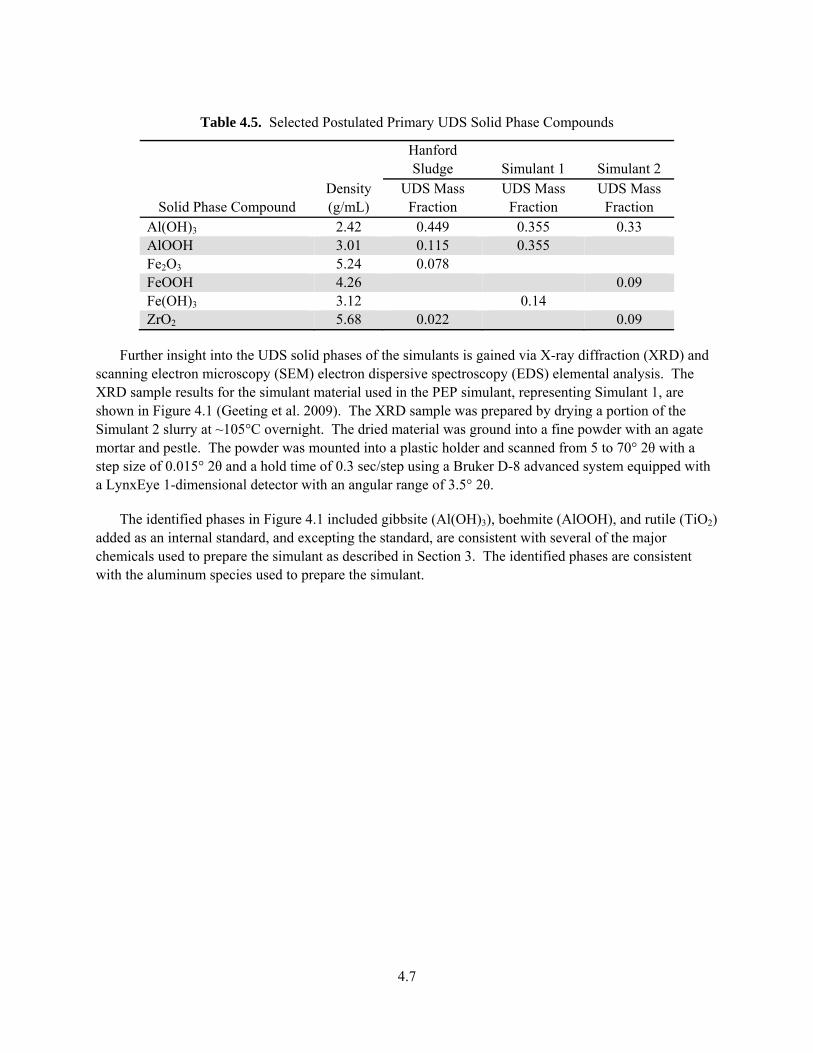
4.7
Table 4.5. Selected Postulated Primary UDS Solid Phase Compounds
Solid Phase Compound Density (g/mL)
Hanford Sludge Simulant 1 Simulant 2
UDS Mass Fraction
UDS Mass Fraction
UDS Mass Fraction
Al(OH)3 2.42 0.449 0.355 0.33 AlOOH 3.01 0.115 0.355 Fe2O3 5.24 0.078 FeOOH 4.26 0.09 Fe(OH)3 3.12 0.14 ZrO2 5.68 0.022 0.09
Further insight into the UDS solid phases of the simulants is gained via X-ray diffraction (XRD) and scanning electron microscopy (SEM) electron dispersive spectroscopy (EDS) elemental analysis. The XRD sample results for the simulant material used in the PEP simulant, representing Simulant 1, are shown in Figure 4.1 (Geeting et al. 2009). The XRD sample was prepared by drying a portion of the Simulant 2 slurry at ~105°C overnight. The dried material was ground into a fine powder with an agate mortar and pestle. The powder was mounted into a plastic holder and scanned from 5 to 70° 2θ with a step size of 0.015° 2θ and a hold time of 0.3 sec/step using a Bruker D-8 advanced system equipped with a LynxEye 1-dimensional detector with an angular range of 3.5° 2θ.
The identified phases in Figure 4.1 included gibbsite (Al(OH)3), boehmite (AlOOH), and rutile (TiO2) added as an internal standard, and excepting the standard, are consistent with several of the major chemicals used to prepare the simulant as described in Section 3. The identified phases are consistent with the aluminum species used to prepare the simulant.
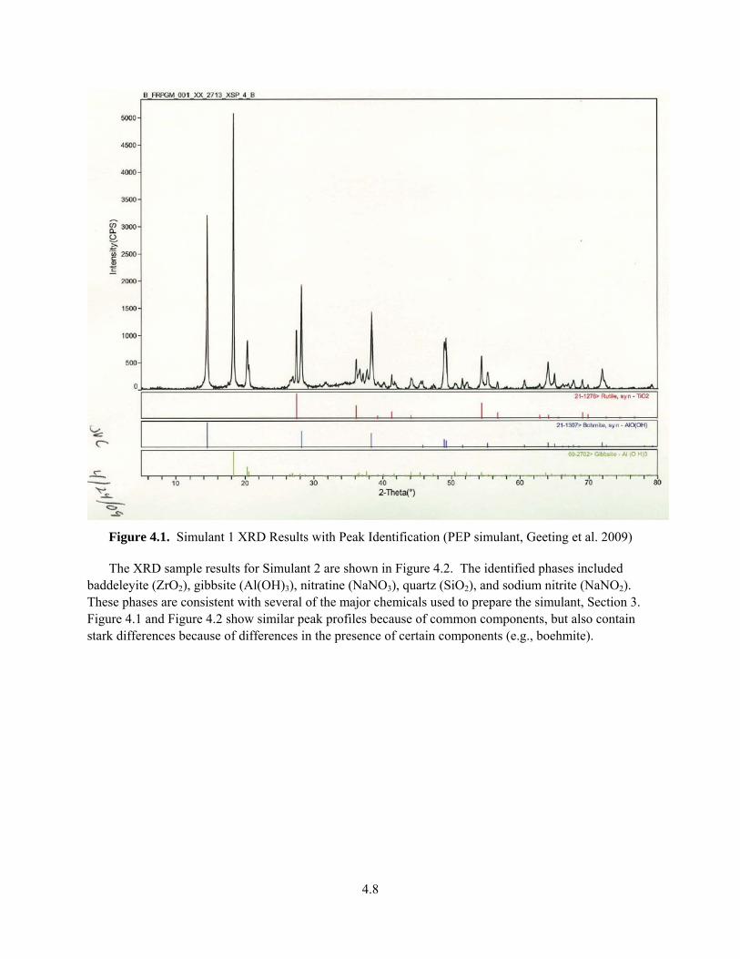
4.8
Figure 4.1. Simulant 1 XRD Results with Peak Identification (PEP simulant, Geeting et al. 2009)
The XRD sample results for Simulant 2 are shown in Figure 4.2. The identified phases included baddeleyite (ZrO2), gibbsite (Al(OH)3), nitratine (NaNO3), quartz (SiO2), and sodium nitrite (NaNO2). These phases are consistent with several of the major chemicals used to prepare the simulant, Section 3. Figure 4.1 and Figure 4.2 show similar peak profiles because of common components, but also contain stark differences because of differences in the presence of certain components (e.g., boehmite).

4.9
x10 3̂
5.0
10.0
15.0In
tens
ity(C
ount
s)
37-1484> Baddeleyite, syn - ZrO2
61-2558> Gibbsite - Al (O H)3
63-3353> Nitratine - Na (N O3)
64-7812> Quartz low - Si O2
06-0392> NaNO2 - Sodium Nitrite
10 20 30 40 50 602-Theta(°)
Figure 4.2. Simulant 2 XRD Results with Peak Identification
The SEM elemental analysis results for Simulant 2 are shown graphically in Figure 4.3 and numerically in Table 4.6. Figure 4.3 shows the SEM image of the sample location from where the elemental analysis data were collected. The numeric data indicate that a substantial majority of the sample contains oxygen and sodium followed by lesser amounts of aluminum and iron and significantly smaller amounts of other simulant components. The data are consistent with the simulant composition (e.g., significant amounts of NaNO3, NaNO2, Al(OH)3, and FeOOH). It is interesting that ZrO2 was identified in the XRD results (Figure 4.2) but was not found during the SEM elemental analysis (Figure 4.4, Table 4.6).
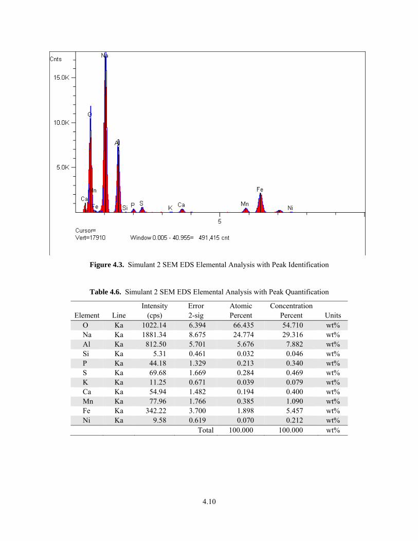
4.10
Figure 4.3. Simulant 2 SEM EDS Elemental Analysis with Peak Identification
Table 4.6. Simulant 2 SEM EDS Elemental Analysis with Peak Quantification
Element Line Intensity
(cps) Error 2-sig
Atomic Percent
Concentration Percent Units
O Ka 1022.14 6.394 66.435 54.710 wt% Na Ka 1881.34 8.675 24.774 29.316 wt% Al Ka 812.50 5.701 5.676 7.882 wt% Si Ka 5.31 0.461 0.032 0.046 wt% P Ka 44.18 1.329 0.213 0.340 wt% S Ka 69.68 1.669 0.284 0.469 wt% K Ka 11.25 0.671 0.039 0.079 wt% Ca Ka 54.94 1.482 0.194 0.400 wt% Mn Ka 77.96 1.766 0.385 1.090 wt% Fe Ka 342.22 3.700 1.898 5.457 wt% Ni Ka 9.58 0.619 0.070 0.212 wt%
Total 100.000 100.000 wt%
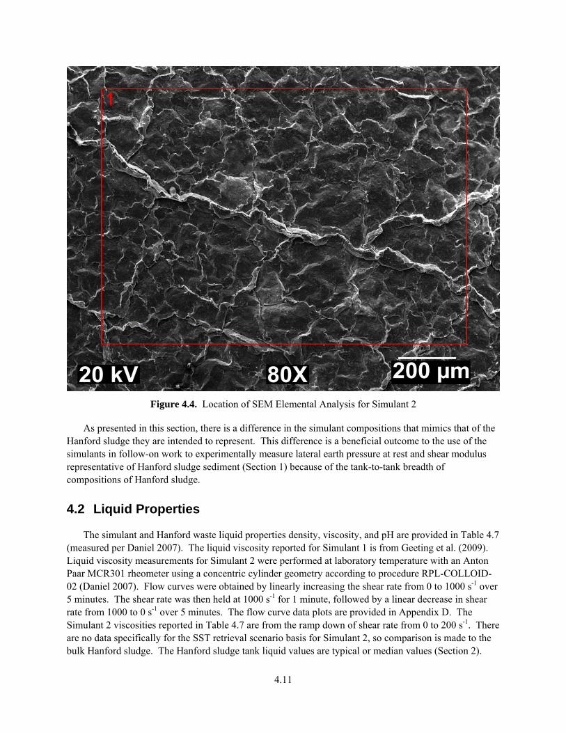
4.11
Figure 4.4. Location of SEM Elemental Analysis for Simulant 2
As presented in this section, there is a difference in the simulant compositions that mimics that of the Hanford sludge they are intended to represent. This difference is a beneficial outcome to the use of the simulants in follow-on work to experimentally measure lateral earth pressure at rest and shear modulus representative of Hanford sludge sediment (Section 1) because of the tank-to-tank breadth of compositions of Hanford sludge.
4.2 Liquid Properties
The simulant and Hanford waste liquid properties density, viscosity, and pH are provided in Table 4.7 (measured per Daniel 2007). The liquid viscosity reported for Simulant 1 is from Geeting et al. (2009). Liquid viscosity measurements for Simulant 2 were performed at laboratory temperature with an Anton Paar MCR301 rheometer using a concentric cylinder geometry according to procedure RPL-COLLOID-02 (Daniel 2007). Flow curves were obtained by linearly increasing the shear rate from 0 to 1000 s-1 over 5 minutes. The shear rate was then held at 1000 s-1 for 1 minute, followed by a linear decrease in shear rate from 1000 to 0 s-1 over 5 minutes. The flow curve data plots are provided in Appendix D. The Simulant 2 viscosities reported in Table 4.7 are from the ramp down of shear rate from 0 to 200 s-1. There are no data specifically for the SST retrieval scenario basis for Simulant 2, so comparison is made to the bulk Hanford sludge. The Hanford sludge tank liquid values are typical or median values (Section 2).
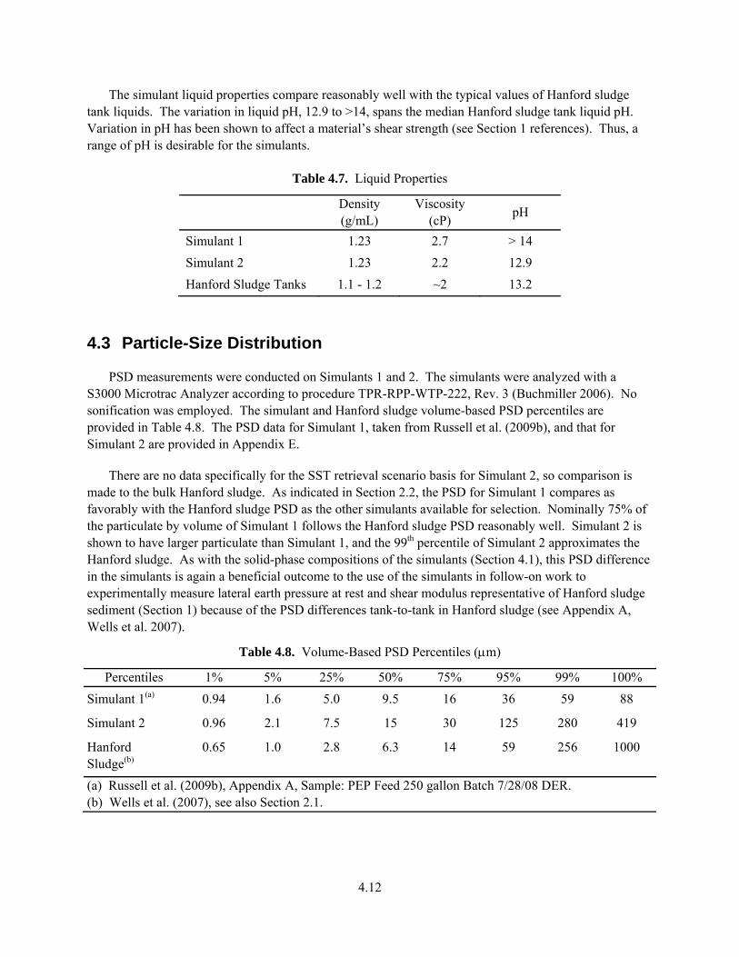
4.12
The simulant liquid properties compare reasonably well with the typical values of Hanford sludge tank liquids. The variation in liquid pH, 12.9 to >14, spans the median Hanford sludge tank liquid pH. Variation in pH has been shown to affect a material’s shear strength (see Section 1 references). Thus, a range of pH is desirable for the simulants.
Table 4.7. Liquid Properties
Density (g/mL)
Viscosity (cP)
pH
Simulant 1 1.23 2.7 > 14
Simulant 2 1.23 2.2 12.9
Hanford Sludge Tanks 1.1 - 1.2 ~2 13.2
4.3 Particle-Size Distribution
PSD measurements were conducted on Simulants 1 and 2. The simulants were analyzed with a S3000 Microtrac Analyzer according to procedure TPR-RPP-WTP-222, Rev. 3 (Buchmiller 2006). No sonification was employed. The simulant and Hanford sludge volume-based PSD percentiles are provided in Table 4.8. The PSD data for Simulant 1, taken from Russell et al. (2009b), and that for Simulant 2 are provided in Appendix E.
There are no data specifically for the SST retrieval scenario basis for Simulant 2, so comparison is made to the bulk Hanford sludge. As indicated in Section 2.2, the PSD for Simulant 1 compares as favorably with the Hanford sludge PSD as the other simulants available for selection. Nominally 75% of the particulate by volume of Simulant 1 follows the Hanford sludge PSD reasonably well. Simulant 2 is shown to have larger particulate than Simulant 1, and the 99th percentile of Simulant 2 approximates the Hanford sludge. As with the solid-phase compositions of the simulants (Section 4.1), this PSD difference in the simulants is again a beneficial outcome to the use of the simulants in follow-on work to experimentally measure lateral earth pressure at rest and shear modulus representative of Hanford sludge sediment (Section 1) because of the PSD differences tank-to-tank in Hanford sludge (see Appendix A, Wells et al. 2007).
Table 4.8. Volume-Based PSD Percentiles (m)
Percentiles 1% 5% 25% 50% 75% 95% 99% 100%
Simulant 1(a) 0.94 1.6 5.0 9.5 16 36 59 88
Simulant 2 0.96 2.1 7.5 15 30 125 280 419
Hanford Sludge(b)
0.65 1.0 2.8 6.3 14 59 256 1000
(a) Russell et al. (2009b), Appendix A, Sample: PEP Feed 250 gallon Batch 7/28/08 DER. (b) Wells et al. (2007), see also Section 2.1.
4.13
4.4 Rheology
The rheology of the simulants is characterized by the Bingham yield stress and consistency, and the shear strength. The Bingham yield stress and consistency were obtained at laboratory temperatures with an Anton Paar MCR301 rheometer using a concentric cylinder geometry under procedure RPL-COLLOID-02 (Daniel 2007). The samples were fully mixed before being introduced into the rheometer. The rheometer was operated in the controlled-rate mode. Flow curves were obtained by linearly increasing the shear rate from 0 to 1000 s-1 over 5 minutes. The shear rate was then held at 1000 s-1 for 1 minute, followed by a linear decrease in shear rate from 1000 to 0 s-1 over 5 minutes. Higher UDS concentrations than the as-prepared (Section 4.1) were achieved via centrifugation (10 minutes at 4500 rpm concentrated Simulant 2 from 0.23 to 0.35 mass fraction UDS).
The Bingham parameters from the shear rate down-curve are provided in Table 4.9 together with the mass fraction of UDS of the analyzed sample. Hanford slurry Bingham parameters at equivalent UDS concentrations are the approximate 95% empirical limits provided in Section 2.1, Figure 2.7 and Figure 2.8. Both simulants exhibited thixotropic and, at the higher UDS concentrations, overshoot behavior as illustrated by the slurry flow curves in Appendix F. Thixotropic behavior is commonly observed in Hanford slurries (e.g., Poloski et al. 2007, Onishi et al. 2003). Overshoot behavior describes the elevated shear stress on the up-curve of the shear rate and will be discussed further in relation to the shear vane measurements presented below.
The lower UDS concentration simulant samples are shown to have Bingham parameters that fall within the 95% empirical limits of the Hanford sludge slurry. The results for the higher UDS concentration simulant samples apparently exceed those of Hanford sludge slurry. However, as noted in Section 2.1, varied waste and sample conditions are represented in the Hanford data, and a trend of increased rheology with increased UDS concentration is expected (see references in Section 1 and the following shear strength discussion). Thus it is expected that the lower Bingham parameters for higher UDS concentrations shown in Figure 2.7 and Figure 2.8 for the Hanford waste are solely a result of the disparate data set. The increasing Bingham parameter trends up to 0.1 mass fraction UDS of Figure 2.7 and Figure 2.8 support the elevated simulant results.
The typical trend of increased simulant rheology with increased UDS concentration is shown in Figure 4.5. Also illustrated in Figure 4.5 is the difference in the simulants’ Bingham parameters for a given UDS concentration. A range of simulant rheology at a given UDS concentration is desirable given the broad Hanford waste variation, Figure 2.7 and Figure 2.8.
The shear strength measurements were obtained using the vane method with a Haake M5 rheometer under procedure RPL-COLLOID-02 (Daniel 2007). Simulant shear-strength measurements are provided in Table 4.10 together with the mass fraction of UDS of the analyzed sample.
It has been shown for a given concentration that the shear strength of clay slurries and other cohesive materials can be a transient property that changes with the time the material remains quiescent. Poloski et al. (2007) summarizes shear strength as a function of quiescent or “gel” time for various gels, soils, chemical slurries, clay slurries, and actual pretreated Hanford waste, and shear strength is shown to increase with quiescent time to an eventual equilibrium shear strength. Equilibrium shear strengths are achieved after quiescent times from hours to weeks depending on the material considered. A clay slurry consisting of 80% kaolin, 20% bentonite by mass in water had a gel time of approximately 4 days. The
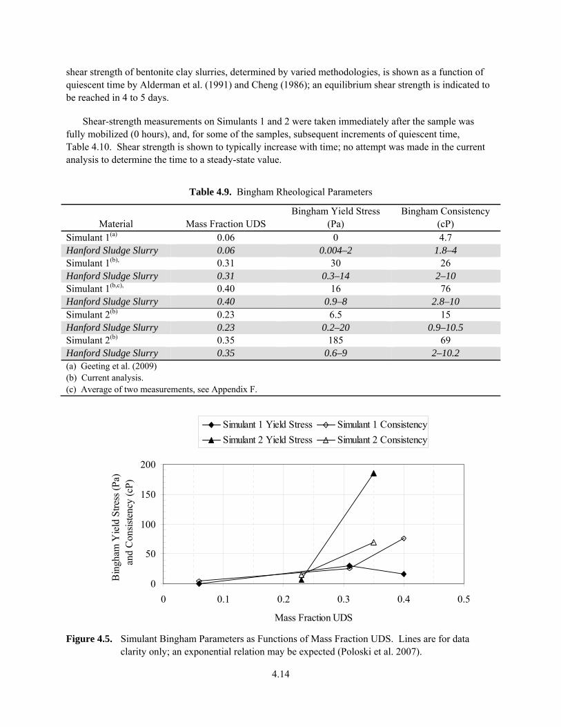
4.14
shear strength of bentonite clay slurries, determined by varied methodologies, is shown as a function of quiescent time by Alderman et al. (1991) and Cheng (1986); an equilibrium shear strength is indicated to be reached in 4 to 5 days.
Shear-strength measurements on Simulants 1 and 2 were taken immediately after the sample was fully mobilized (0 hours), and, for some of the samples, subsequent increments of quiescent time, Table 4.10. Shear strength is shown to typically increase with time; no attempt was made in the current analysis to determine the time to a steady-state value.
Table 4.9. Bingham Rheological Parameters
Material Mass Fraction UDS Bingham Yield Stress
(Pa) Bingham Consistency
(cP) Simulant 1(a) 0.06 0 4.7 Hanford Sludge Slurry 0.06 0.004–2 1.8–4 Simulant 1(b), 0.31 30 26 Hanford Sludge Slurry 0.31 0.3–14 2–10 Simulant 1(b,c), 0.40 16 76 Hanford Sludge Slurry 0.40 0.9–8 2.8–10 Simulant 2(b) 0.23 6.5 15 Hanford Sludge Slurry 0.23 0.2–20 0.9–10.5 Simulant 2(b) 0.35 185 69 Hanford Sludge Slurry 0.35 0.6–9 2–10.2 (a) Geeting et al. (2009) (b) Current analysis. (c) Average of two measurements, see Appendix F.
0
50
100
150
200
0 0.1 0.2 0.3 0.4 0.5
Mass Fraction UDS
Bin
gham
Yie
ld S
tres
s (P
a)
an
d C
onsi
sten
cy (
cP)
Simulant 1 Yield Stress Simulant 1 Consistency
Simulant 2 Yield Stress Simulant 2 Consistency
Figure 4.5. Simulant Bingham Parameters as Functions of Mass Fraction UDS. Lines are for data clarity only; an exponential relation may be expected (Poloski et al. 2007).
4.15
Table 4.10. Shear Strength
Material Mass Fraction UDS Shear Strength (Pa), Quiescent Time Simulant 1 0.31 34.3, 0 hours Hanford Sludge Slurry 0.31 160–6000, <50 years Simulant 1 0.40 921, 0 hours
1088, 1 hour 1383, 24 hours
Hanford Sludge Slurry 0.40 70–9000, <50 years Simulant 2 0.23 8.7, 0 hours
21.6, 24 hours Hanford Sludge Slurry 0.23 300–3100, <50 years Simulant 2 0.35 775, 0 hours
752, 1 hour 1133, 24 hours
Hanford Sludge Slurry 0.35 70–9000, <50 years
The Hanford sludge sediment shear strengths at equivalent UDS concentrations provided in Table 4.10 are the approximate 95% empirical limits provided in Section 2.1, Figure 2.11. Even with the significant quiescent time differences, the simulants fall within the broad shear-strength range of the Hanford sludge sediment. As with the Bingham rheological parameters, varied waste and sample conditions are represented by the Hanford data.
The trend of increased shear strength with increased UDS concentration for the simulants is shown in Figure 4.6 for the 0-hours measurements. Actual waste shear-strength and UDS-concentration relations for T-204, B-203, and AZ-101 from Gauglitz et al. (2009) are included.
Numerous experimental studies related to the storage and retrieval of waste from the large underground Hanford storage tanks have employed clay slurries as simulants to represent the waste of interest. These studies have included investigations of gas retention and release (Gauglitz et al. 1994, Gauglitz et al. 1995, Gauglitz et al. 1996, Stewart et al. 1996, etc.), sediment mobilization (Powell et al. 1995, Enderlin et al. 2003, Bontha et al. 2005, Kurath et al. 2007, etc.), and slurry transport (Poloski et al. 2009). Gauglitz and Aiken (1997) developed a method to obtain shear-strength estimates for Hanford sediment via visual observation of waste core extrusion behavior. To do so, they employed bentonite slurry to mimic ductile waste behavior and Kaolin/Ludox slurry to mimic brittle waste behavior. The correlations for kaolin and kaolin/bentonite from (Rassat et al. 2003) are presented in Figure 4.2 together with bentonite data (16 hour quiescent time) from Alderman et al (1991).
Simulants 1 and 2 are shown to have slopes (note log plot) like the B-203 and T-204 data and are bounded by the previously employed clay simulants. The shear strength-UDS mass fraction relation for Simulant 1 is
Sw559.36e0004.0 (4.2) and
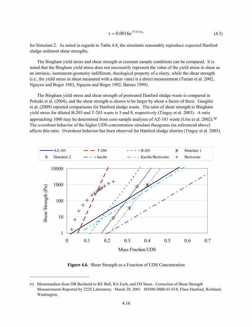
4.16
Sw413.37e0016.0 (4.3) for Simulant 2. As noted in regards to Table 4.8, the simulants reasonably reproduce expected Hanford sludge sediment shear strengths.
The Bingham yield stress and shear strength at constant sample conditions can be compared. It is noted that the Bingham yield stress does not necessarily represent the value of the yield stress in shear as an intrinsic, instrument-geometry indifferent, rheological property of a slurry, while the shear strength (i.e., the yield stress in shear measured with a shear vane) is a direct measurement (Turian et al. 2002, Nguyen and Boger 1983, Nguyen and Boger 1992, Barnes 1999).
The Bingham yield stress and shear strength of pretreated Hanford sludge waste is compared in Poloski et al. (2004), and the shear strength is shown to be larger by about a factor of three. Gauglitz et al. (2009) reported comparisons for Hanford sludge waste. The ratio of shear strength to Bingham yield stress for diluted B-203 and T-203 waste is 5 and 8, respectively (Tingey et al. 2003). A ratio
approaching 1000 may be determined from core-sample analyses of AZ-101 waste (Urie et al. 2002).(a) The overshoot behavior of the higher UDS concentration simulant rheograms (as referenced above) affects this ratio. Overshoot behavior has been observed for Hanford sludge slurries (Tingey et al. 2003).
1
10
100
1000
10000
0 0.1 0.2 0.3 0.4 0.5 0.6 0.7
Mass Fraction UDS
She
ar S
tren
gth
(Pa)
.
AZ-101 T-204 B-203 Simulant 1
Simulant 2 kaolin Kaolin/Bentonite Bentonite
Figure 4.6. Shear Strength as a Function of UDS Concentration
(a) Memorandum from DB Bechtold to KE Bell, RA Esch, and FH Steen. Correction of Shear Strength Measurements Reported by 222S Laboratory. March 28, 2001. 8D500-DBB-01-018, Fluor Hanford, Richland, Washington.
4.17
Speers et al. (1987) refer to “gel strength” as “the shear strength overshoot which occurs in a previously resting fluid which is suddenly sheared.” For the current analysis, the simulant material was completely mobilized immediately before being introduced into the rheometer, and the measurements were immediately taken once the sample was in the rheometer. Baudez (2006) concluded that the initial stress overshoot is highly dependent on the shear-rate increment profile and the data sampling.
The Bingham yield stress (low UDS concentrations) or approximate peak shear stress (high UDS concentrations) from the simulant ramp-up flow curves of Appendix F is provided in Table 4.11 together with the Bingham yield stress and shear strength at 0 hours from Table 4.9 and Table 4.10, respectively. Good agreement (Bingham yield stress to shear strength ratio is ~ 1) is shown for the lower UDS concentration conditions. These comparisons potentially show that at the lower UDS concentrations, the simulants behave as a Bingham plastic as both the indirect and direct measures of the yield stress in shear are in close agreement.
The peak shear stress (flow curve ramp-up) is shown to compare much more favorably with the shear strength than the Bingham yield stress (flow curve ramp-down) for the higher UDS concentrations. The rheogram peak shear-stress to shear-strength ratios for Simulants 1 and 2 are in remarkable agreement at 1.25 and 1.35, respectively. This comparison may suggest that the overshoot behavior from the rheograms is not solely an artifact of the indirect measurement method.
The different rheological behavior (i.e., Table 4.9 through Table 4.11) of the simulants is appropriate given the differences of Hanford sludge and the use of these simulants in follow-on work to experimentally measure lateral earth pressure at rest and shear modulus representative of Hanford sludge sediment (see Section 1).
Table 4.11. Bingham Yield Stress and Shear-Strength Comparison
Material Mass Fraction UDS Bingham Yield
Stress (Pa) Ramp-up Shear
Stress (Pa)(a) Shear Strength
(Pa)
Simulant 1 0.31 30 31.5 34.3
Simulant 1 0.40 16(b) 735(b) 921
Simulant 2 0.23 6.5 7.4 8.7
Simulant 2 0.35 185 575 775
(a) Approximate values from flow curve ramp-ups, Appendix F. Simulant 1 and 2 low UDS concentrations, Bingham yield stress, Simulant 1 and 2 high UDS concentrations, peak shear stress.
(b) Average of two measurements, see Appendix F.
4.5 Shear Modulus
The shear modulus is the slope of the initial linear portion of a shear stress-shear strain curve and is a measure of the material’s stiffness in shear. Alderman et al. (1991) provide an extension of the vane technique to determine the shear modulus, G, as
4.18
2C
2 R
1
R
1
dt
dT
H4
1G (4.4)
where = angular velocity of the vane H = vane height dT/dt = slope of the linear portion of the torque-time curve resulting from the Hookean
elastic response of the sample R = vane radius RC radius of the sample container. Alderman et al. demonstrated good agreement between the shear modulus determined via the vane technique and Equation (4.4) and low-strain oscillation measurements using a Bohlin VOR rheometer in a 9.99 wt% bentonite clay suspension.
Equation (4.4) is applied to the shear-vane measurement data of Table 4.10. In addition to the vane dimension and placement in sample requirements synonymous with RPL-COLLOID-02 (Daniel 2007), Equation (4.4) requires that the vane be placed near the center of the sample container radially, and the container diameter should be about three times larger than the vane diameter. These conditions were met in the current analysis. The vane rotational speed was 0.03 revolutions per second for all measurements, a 1.6-cm × 1.6-cm (diameter × height) vane was used for the lower UDS concentration samples, and a 0.6-cm × 0.6-cm vane for the higher UDS concentration samples. Simulant 1 was measured in a 5-cm-diameter container, and Simulant 2 was in a 5-cm-diameter container for the lower UDS concentration measurements, 6 cm for the higher.
The shear modulus is shown to increase (Simulant 1, 1 hour to 24 hours does not follow trend) with both the UDS concentration and quiescent time as expected (Alderman et al. 1991), Table 4.12. Comparison of shear strength and shear modulus as functions of the UDS concentration is made in Figure 4.7. As noted in Section 1, there are no in situ shear modulus data for the Hanford sediment. Thus, the bentonite clay shear strength (see Figure 4.6) and shear modulus of Alderman et al. (1991) are used for comparison.
The simulant data presented in Figure 4.7 are for the 0 hours measurements, and the bentonite clay data are from the fit to 16-hour quiescent time measurements. At a given UDS concentration, the shear modulus for the simulants is shown to exceed the shear strength by a factor of approximately 2 or greater. The shear modulus of the bentonite clay increasingly exceeds the shear strength starting at UDS mass fractions greater than approximately 0.1.
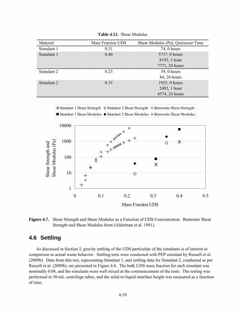
4.19
Table 4.12. Shear Modulus
Material Mass Fraction UDS Shear Modulus (Pa), Quiescent Time Simulant 1 0.31 74, 0 hours Simulant 1 0.40 5737, 0 hours
8193, 1 hour 7771, 24 hours
Simulant 2 0.23 39, 0 hours 84, 24 hours
Simulant 2 0.35 1925, 0 hours 2492, 1 hour
4574, 24 hours
1
10
100
1000
10000
0 0.1 0.2 0.3 0.4 0.5
Mass Fraction UDS
She
ar S
tren
gth
and
S
hear
Mod
ulus
(P
a) .
Simulant 1 Shear Strength Simulant 2 Shear Strength Bentonite Shear Strength
Simulant 1 Shear Modulus Simulant 2 Shear Modulus Bentonite Shear Modulus
Figure 4.7. Shear Strength and Shear Modulus as a Function of UDS Concentration. Bentonite Shear Strength and Shear Modulus from (Alderman et al. 1991).
4.6 Settling
As discussed in Section 2, gravity settling of the UDS particulate of the simulants is of interest in comparison to actual waste behavior. Settling tests were conducted with PEP simulant by Russell et al. (2009b). Data from this test, representing Simulant 1, and settling data for Simulant 2, conducted as per Russell et al. (2009b), are presented in Figure 4.8. The bulk UDS mass fraction for each simulant was nominally 0.04, and the simulants were well mixed at the commencement of the tests. The testing was performed in 50-mL centrifuge tubes, and the solid-to-liquid interface height was measured as a function of time.
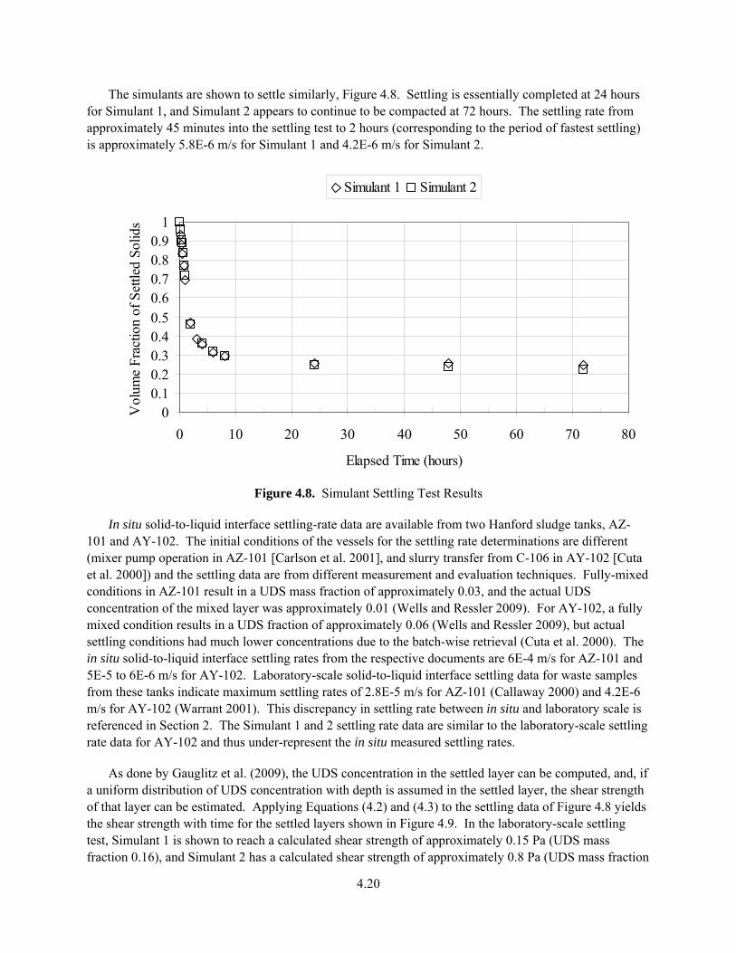
4.20
The simulants are shown to settle similarly, Figure 4.8. Settling is essentially completed at 24 hours for Simulant 1, and Simulant 2 appears to continue to be compacted at 72 hours. The settling rate from approximately 45 minutes into the settling test to 2 hours (corresponding to the period of fastest settling) is approximately 5.8E-6 m/s for Simulant 1 and 4.2E-6 m/s for Simulant 2.
00.10.20.30.40.50.60.70.80.9
1
0 10 20 30 40 50 60 70 80
Elapsed Time (hours)
Vol
ume
Fra
ctio
n of
Set
tled
Sol
ids
Simulant 1 Simulant 2
Figure 4.8. Simulant Settling Test Results
In situ solid-to-liquid interface settling-rate data are available from two Hanford sludge tanks, AZ-101 and AY-102. The initial conditions of the vessels for the settling rate determinations are different (mixer pump operation in AZ-101 [Carlson et al. 2001], and slurry transfer from C-106 in AY-102 [Cuta et al. 2000]) and the settling data are from different measurement and evaluation techniques. Fully-mixed conditions in AZ-101 result in a UDS mass fraction of approximately 0.03, and the actual UDS concentration of the mixed layer was approximately 0.01 (Wells and Ressler 2009). For AY-102, a fully mixed condition results in a UDS fraction of approximately 0.06 (Wells and Ressler 2009), but actual settling conditions had much lower concentrations due to the batch-wise retrieval (Cuta et al. 2000). The in situ solid-to-liquid interface settling rates from the respective documents are 6E-4 m/s for AZ-101 and 5E-5 to 6E-6 m/s for AY-102. Laboratory-scale solid-to-liquid interface settling data for waste samples from these tanks indicate maximum settling rates of 2.8E-5 m/s for AZ-101 (Callaway 2000) and 4.2E-6 m/s for AY-102 (Warrant 2001). This discrepancy in settling rate between in situ and laboratory scale is referenced in Section 2. The Simulant 1 and 2 settling rate data are similar to the laboratory-scale settling rate data for AY-102 and thus under-represent the in situ measured settling rates.
As done by Gauglitz et al. (2009), the UDS concentration in the settled layer can be computed, and, if a uniform distribution of UDS concentration with depth is assumed in the settled layer, the shear strength of that layer can be estimated. Applying Equations (4.2) and (4.3) to the settling data of Figure 4.8 yields the shear strength with time for the settled layers shown in Figure 4.9. In the laboratory-scale settling test, Simulant 1 is shown to reach a calculated shear strength of approximately 0.15 Pa (UDS mass fraction 0.16), and Simulant 2 has a calculated shear strength of approximately 0.8 Pa (UDS mass fraction
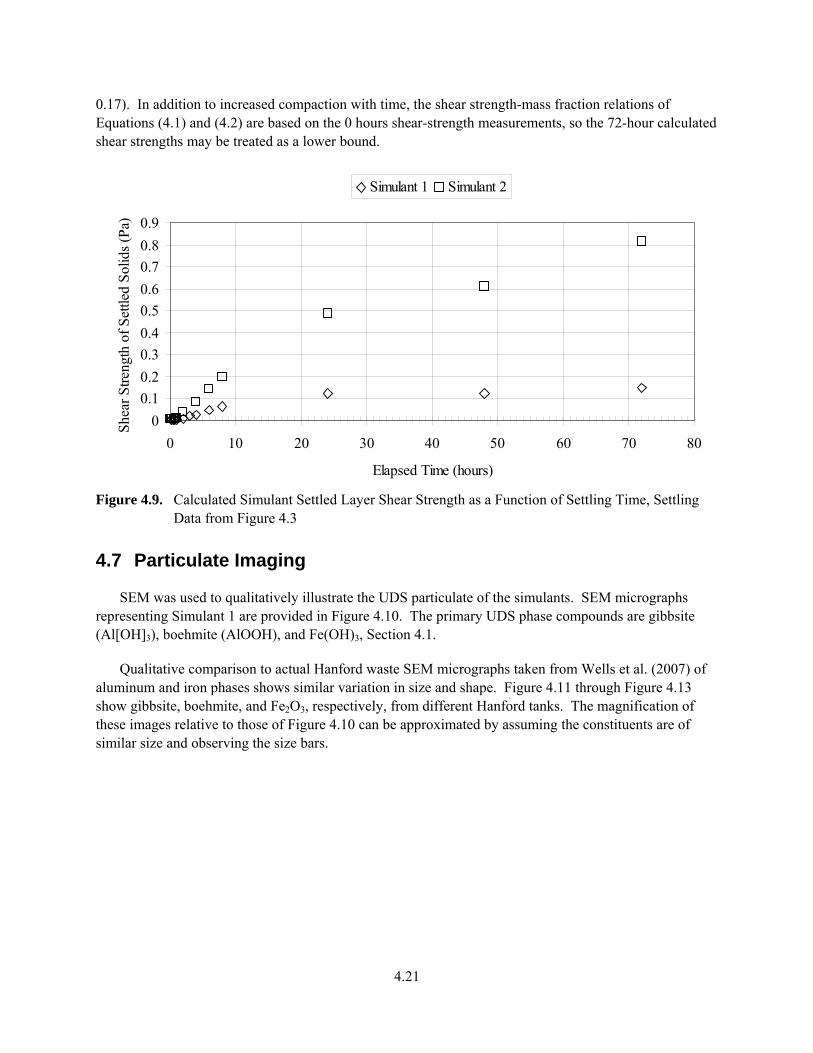
4.21
0.17). In addition to increased compaction with time, the shear strength-mass fraction relations of Equations (4.1) and (4.2) are based on the 0 hours shear-strength measurements, so the 72-hour calculated shear strengths may be treated as a lower bound.
0
0.1
0.2
0.3
0.4
0.5
0.6
0.7
0.8
0.9
0 10 20 30 40 50 60 70 80
Elapsed Time (hours)
She
ar S
tren
gth
of S
ettle
d S
olid
s (P
a)
Simulant 1 Simulant 2
Figure 4.9. Calculated Simulant Settled Layer Shear Strength as a Function of Settling Time, Settling Data from Figure 4.3
4.7 Particulate Imaging
SEM was used to qualitatively illustrate the UDS particulate of the simulants. SEM micrographs representing Simulant 1 are provided in Figure 4.10. The primary UDS phase compounds are gibbsite (Al[OH]3), boehmite (AlOOH), and Fe(OH)3, Section 4.1.
Qualitative comparison to actual Hanford waste SEM micrographs taken from Wells et al. (2007) of aluminum and iron phases shows similar variation in size and shape. Figure 4.11 through Figure 4.13 show gibbsite, boehmite, and Fe2O3, respectively, from different Hanford tanks. The magnification of these images relative to those of Figure 4.10 can be approximated by assuming the constituents are of similar size and observing the size bars.
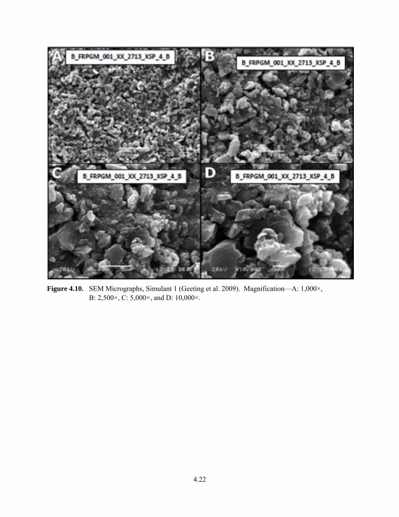
4.22
Figure 4.10. SEM Micrographs, Simulant 1 (Geeting et al. 2009). Magnification—A: 1,000×, B: 2,500×, C: 5,000×, and D: 10,000×.
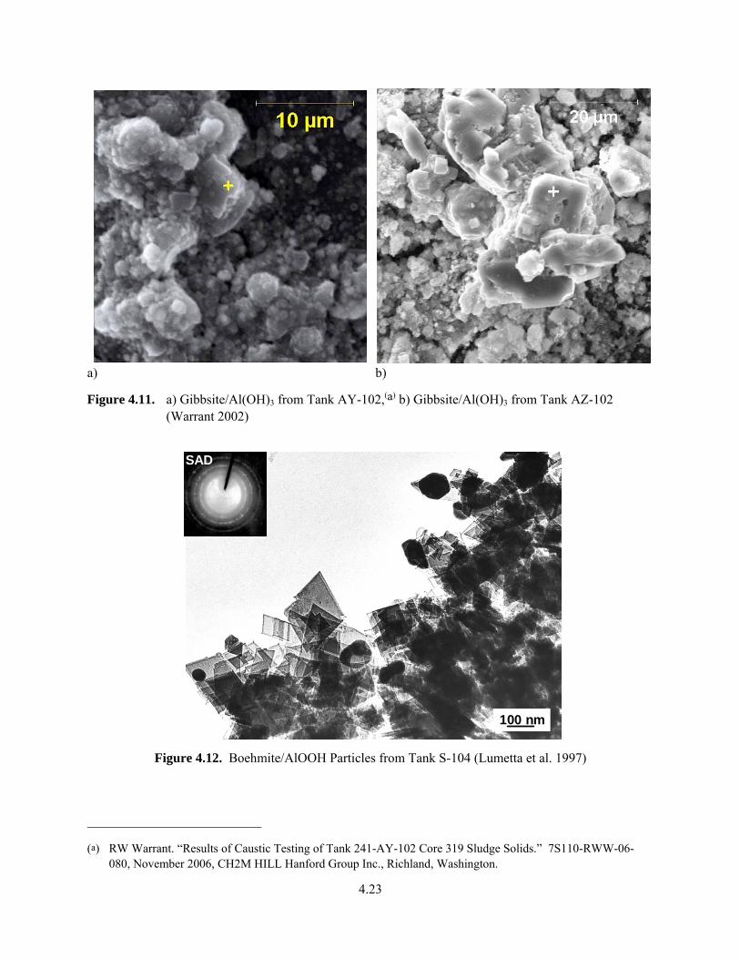
4.23
a) b)
Figure 4.11. a) Gibbsite/Al(OH)3 from Tank AY-102,(a) b) Gibbsite/Al(OH)3 from Tank AZ-102 (Warrant 2002)
SAD
100 nm
Figure 4.12. Boehmite/AlOOH Particles from Tank S-104 (Lumetta et al. 1997)
(a) RW Warrant. “Results of Caustic Testing of Tank 241-AY-102 Core 319 Sludge Solids.” 7S110-RWW-06-080, November 2006, CH2M HILL Hanford Group Inc., Richland, Washington.
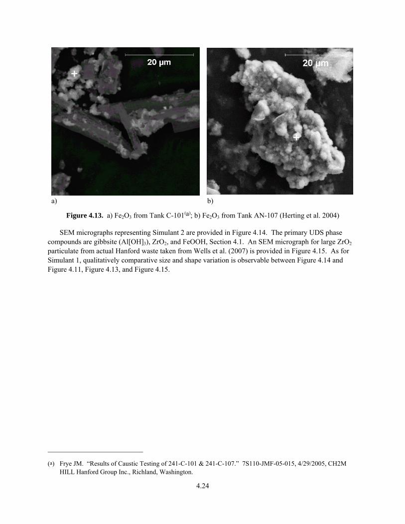
4.24
a) b)
Figure 4.13. a) Fe2O3 from Tank C-101(a); b) Fe2O3 from Tank AN-107 (Herting et al. 2004)
SEM micrographs representing Simulant 2 are provided in Figure 4.14. The primary UDS phase compounds are gibbsite (Al[OH]3), ZrO2, and FeOOH, Section 4.1. An SEM micrograph for large ZrO2 particulate from actual Hanford waste taken from Wells et al. (2007) is provided in Figure 4.15. As for Simulant 1, qualitatively comparative size and shape variation is observable between Figure 4.14 and Figure 4.11, Figure 4.13, and Figure 4.15.
(a) Frye JM. “Results of Caustic Testing of 241-C-101 & 241-C-107.” 7S110-JMF-05-015, 4/29/2005, CH2M HILL Hanford Group Inc., Richland, Washington.
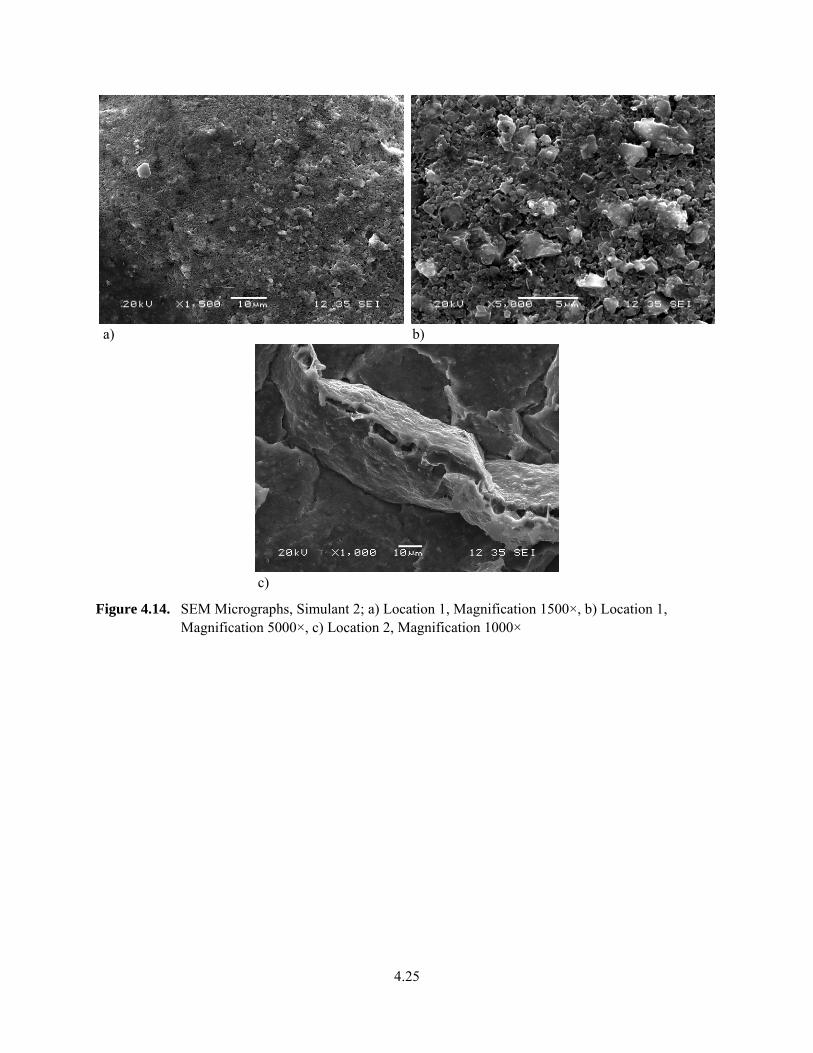
4.25
a) b)
c)
Figure 4.14. SEM Micrographs, Simulant 2; a) Location 1, Magnification 1500×, b) Location 1, Magnification 5000×, c) Location 2, Magnification 1000×
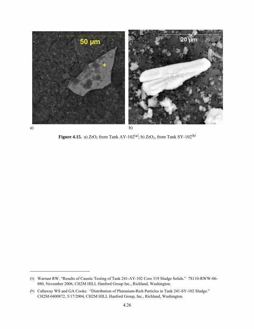
4.26
a) b)
Figure 4.15. a) ZrO2 from Tank AY-102(a); b) ZrO2, from Tank SY-102(b)
(a) Warrant RW. “Results of Caustic Testing of Tank 241-AY-102 Core 319 Sludge Solids.” 7S110-RWW-06-080, November 2006, CH2M HILL Hanford Group Inc., Richland, Washington.
(b) Callaway WS and GA Cooke. “Distribution of Plutonium-Rich Particles in Tank 241-SY-102 Sludge.” CH2M-0400872, 5/17/2004, CH2M HILL Hanford Group, Inc., Richland, Washington.
5.1
5.0 Summary
The objective of this work was to select or develop two chemical sludge simulants to be used in follow-on work to experimentally measure lateral earth pressure at rest and shear modulus representative of Hanford sludge sediment. Two chemical simulants, one representing the Hanford sludge as a whole and the other a specific SST retrieval scenario (C-104, C-111, and C-112 retrieval into AN-101) have been selected to meet this objective.
Simulant 1 is chosen from Hanford sludge simulants that have previously been produced and characterized. The selection is based on comparison to actual Hanford sludge chemical and physical properties. Simulant 2 is developed based upon the chemistry of the specific SST retrieval scenario.
The sludge parameters to be measured in follow-on work, lateral earth pressure at rest, and shear modulus are expected to be influenced by the chemical and physical properties of the sludge material. Simulants 1 and 2 are shown to have chemical and physical properties that match well with all of the Hanford sludge parameters considered. The uniqueness of the simulants with respect to each other for some of the parameters considered is a beneficial outcome given the broad variation of Hanford waste.

6.1
6.0 References
Alderman NJ, GH Meeten, and JD Sherwood. 1991. “Vane Rheometry of Bentonite Gels.” Journal of Non-Newtonian Fluid Mechanics 39:291–310.
Ancey C and H Jorrot. 2001. “Yield Stress for Particle Suspensions Within a Clay Dispersion.” Journal of Rheology 45(2):297–319.
Barnes HA and QD Nguyen. 2001. “Rotating Vane Rheometry - A Review.” Journal of Non-Newtonian Fluid Mechanics 989:1–14.
Barnes HA. 1999. “The Yield Stress—A Review or ‘’—Everything Flows?” Journal of Non-Newtonian Fluid Mechanics 81: 133–178.
Baudez J-C. 2006. “About Peak and Loop in Sludge Rheograms.” Journal of Environmental Management 78:232-239.
Bontha JR, GR Golcar, and N Hammigan. 2000. Demonstration and Optimization of BNFL's Pulsed Jet Mixing and RFD Sampling Systems Performance Using NCAW Simulant. PNWD-3054 (BNFL-RPT-048 Rev. 0), Battelle—Pacific Northwest Division, Richland, Washington.
Bontha JR, TE Michener, DS Trent, JM Bates, and MD Johnson. 2003. Development and Assessment of the TEMPEST CFD Model of the Pulsed Jet Mixing Systems. PNWD-3261 (WTP-RPT-061 Rev. 0), Battelle—Pacific Northwest Division, Richland, Washington.
Bontha JR, CW Stewart, DE Kurath, PA Meyer, ST Arm, CE Guzman-Leong, MS Fountain, M Friedrich, SA Hartley, LK Jagoda, CD Johnson, KS Koschik, DL Lessor, F Nigl, RL Russell, GL Smith, W Yantasee, and ST Yokuda. 2005. Technical Basis for Predicting Mixing and Flammable Gas Behavior in the Ultrafiltration Feed Process and High-Level Waste Lag Storage Vessels with Non-Newtonian Slurries. PNWD-3676 (WTP-RPT-132, Rev. 0), Pacific Northwest National Laboratory, Richland, Washington.
Buchmiller WC. 2006. S3000 Microtrac Particle Size Analyzer. TPR-RPP-WTP-222, Rev. 3, Pacific Northwest National Laboratory, Richland, Washington.
Buscall R, IJ McGowan, PDA Mills, RF Stewart, D Sutton, LR White, and GE Yates. 1987. “The Rheology of Strongly Flocculated Suspensions.” Journal of Non-Newtonian Fluid Mechanics 24:183–202.
Callaway WS. 2000. Results of Retrieval Testing of Sludge from Tank 241-AZ-101. HNF-7078, Rev. 0, Fluor Hanford, Richland, Washington.
Carlson AB, PJ Certa, TM Hohl, JR Bellomy III, TW Crawford, DC Hedengren, AM Templeton, HS Fisher, SJ Greenwood, DG Douglas, and WJ Ulbright Jr. 2001. Test Report, 241-AZ-101 Mixer Pump Test. RPP-6548, Rev. 1, Numatec Hanford Corporation, Richland, Washington.
6.2
Certa PJ and MN Wells. 2009. River Protection Project System Plan. ORP-11242 Rev. 4. Office of River Protection, Richland, Washington.
Channell GM and CF Zukoski. 1997. “Shear and Compressive Rheology of Aggregated Alumina Suspensions.” AIChE Journal 43(7):1700–1708.
Cheng D C-H. 1986. “Yield Stress: A Time Dependent Property and How to Measure It.” Rheological Acta 25:542–554.
Cowley WL, JL Huckaby, LA Mahoney, GR Golcar, KM Krupka, DS Sklarew, and DJ Geniesse. 2003. Chemical Source Terms for Tank Farms Safety Analyses. RPP-8369 Rev. 2, CH2M HILL Hanford Group, Inc., Richland, Washington.
Craig RF. 2004. “Craig's Soil Mechanics.” ISBN 0-415-32702-4. Spon Press, New York, New York.
Cuta JM, KG Carothers, DW Damschen, WL Kuhn, JA Lechelt, K Sathyanarayana, and LA Stauffer. 2000. Review of Waste Retrieval Sluicing System Operations and Data for Tanks 241-C-016 and 241-AY-102. PNNL-13319, Pacific Northwest National Laboratory, Richland, Washington.
Daniel RC. 2007. PNNL Technical Procedure, "Measurement of Physical and Rheological Properties of Solutions, Slurries and Sludges." RPL-COLLOID-02 Rev. 1, Pacific Northwest National Laboratory, Richland, Washington.
Enderlin CW, G Terrones, CJ Bates, BK Hatchell, B Adkins. 2003. Recommendations for Advanced Design Mixer Pump Operation in Savannah River Site Tank 18F. PNNL-14443, Pacific Northwest National Laboratory, Richland, Washington.
Gauglitz PA, and JT Aikin. 1997. Waste Behavior During Horizontal Extrusion: Effect of Waste Strength for Bentonite and Kaolin/Ludox Simulants and Strength Estimates for Wastes from Hanford Tanks 241-SY-103, AW-101, AN-103, and S-102. PNNL-11706, Pacific Northwest National Laboratory, Richland, Washington.
Gauglitz PA, LA Mahoney, DP Mendoza, and MC Miller. 1994. Mechanisms of Gas Bubble Retention. PNL-10120, Pacific Northwest Laboratory, Richland, Washington.
Gauglitz PA, RR Shah, SD Rassat, LA Mahoney, and MR Powell. 1995. Gas Bubble Retention and Its Effects on Waste Properties: Retention Mechanisms, Viscosity, and Tensile and Shear Strengths. PNL-10740, Pacific Northwest Laboratory, Richland, Washington.
Gauglitz PA, SD Rassat, PR Bredt, JH Konynenbelt, SM Tingey, and DP Mendoza. 1996. Mechanisms of Gas Bubble Retention and Release: Results for Hanford Waste Tanks 241 S 102 and 241 SY 103 and Single Shell Tank Simulants. PNNL 11298, Pacific Northwest National Laboratory, Richland, Washington.
Gauglitz PA, BE Wells, JA Fort, and PA Meyer. 2009. An Approach to Understanding Cohesive Slurry Settling, Mobilization, and Hydrogen Gas Retention in Pulsed Jet Mixed Vessels. PNNL-17707, WTP-RPT-177, Rev. 0, Pacific Northwest National Laboratory, Richland, Washington.
6.3
Geeting JGH, EC Golovich, DE Kurath, OP Bredt, CE Guzman-Leong, GJ Sevigny, CA Burns, GB Josephson, and RL Aaberg. 2009. Pretreatment Engineering Platform (PEP) Integrated Test B Run Report - Caustic and Oxidative Leaching in UFP-VSL-T02A. PNNL-18723, WTP-RPT-192, Rev. 0, Pacific Northwest National Laboratory, Richland, Washington.
Gephart RE and RE Lundgren. 2005. Hanford Tank Cleanup: A guide to Understanding the Technical Issues. PNL-10773. Pacific Northwest Laboratory, Richland, Washington.
Golcar GR, KP Brooks, JG Darab, JM Davis, and LK Jagoda. 2000. Development of Inactive High Level Waste Envelope D Simulants for Sealed Crossflow Filtration Testing. PNWD-3042, BNFL-RPT-033 Rev. 0, Battelle—Pacific Northwest Division, Richland, Washington.
Hansen EK, RE Eibling, and TB Calloway, Jr. 2001. Mixing Envelope D Sludge with LAW Intermediate Products with and without Glass Formers. WSRC-TR-2001-00203, Rev. 0, SRT-RPP-2001-00051, Rev. 0. Westinghouse Savannah River Company, Aiken, South Carolina.
Hedengren DC, KM Hodgson, WB Barton, CW Stewart, JM Cuta, and BE Wells. 2000. Data Observations on Double-Shell Flammable Gas Watch List Tank Behavior. RPP-6655, CH2MHILL Hanford Group, Inc., Richland, Washington.
Herting DL, GA Cooke, and RW Warrant. 2004. Hanford Tank 241-AN-107 Solid Phase Characterization. RPP-20018, CH2M HILL Hanford Group, Inc., Richland, Washington.
Jaky J. 1948. “Pressure in Soils.” In: The Second International Conference on Soil Mechanics and Foundation Engineering, London, Vol. 1, 103–107.
Kurath DE, PA Meyer, JR Bontha, AP Poloski, JA Fort, WH Combs, WC Buchmiller, ID Welch, and MD Bleich. 2007. Assessment of Pulse Tube Mixing for Vessels Containing Non-Newtonian Slurries. PNWD-3827 (WTP-RPT-155, Rev. 0), Pacific Northwest National Laboratory, Richland, Washington.
Kurath DE, PW Eslinger, SM Barnes, RL Aaberg, BD Hanson, JL Huckaby, EC Golovich, PM Aker, MJ Minette, JM Billing, SD Rassat, CE Guzman-Leong, DL Baldwin, PS Sundar, CF Brown, ML Kimura, BM Rapko, GJ Josephson, JGH Geeting, SK Sundaram, LA Mahoney, JJ Toth, GJ Sevigny, RP Pires, PP Schonewill, ST Yokuda, AJ Casella, BE Wells, RC Daniel, EBK Baer, JR Bontha, and OP Bredt. 2009. Pretreatment Engineering Platform Phase 1 Final Test Report. PNNL-18894, WTP-RPT-197 Rev. 0, Pacific Northwest National Laboratory, Richland, Washington.
Lumetta GJ, IE Burgeson, MJ Wagner, J Liu, and YL Chen. 1997. Washing and Caustic Leaching of Hanford Tank Sludge: Results of FY1997 Studies. PNNL-11636, Pacific Northwest National Laboratory, Richland, Washington.
Meyer PA and CW Stewart. 2001. Preventing Buoyant Displacement Gas Release Events in Hanford Double-Shell Waste Tanks. PNNL-13337, Pacific Northwest National Laboratory, Richland, Washington.
6.4
Meyer PA, JA Bamberger, CW Enderlin, JA Fort, BE Wells, SK Sundaram, PA Scott, MJ Minette, GL Smith, CA Burns, MS Greenwood, GP Morgen, EBK Baer, SF Snyder, M White, GF Piepel, BG Amidan, A Heredia-Langner. 2009. Pulse Jet Mixing tests with Noncohesive Solids. PNNL-18098, WTP-RPT-182, Rev. 0, Pacific Northwest National Laboratory, Richland, Washington.
Naeini SA and MH Baziar. 2004. “Effect of Fines Content on Steady-State Strength of Mixed and Layered Samples of Sand.” Soil Dynamics and Earthquake Engineering 24:181–187.
Nquyen QD and DV Boger. 1983. “Yield Stress Measurement for Concentrated Suspensions.” Journal of Rheology 27(4):321–349.
Nguyen QD and DV Boger. 1992. “Measuring the Flow Properties of Yield Stress Fluids.” Annual Review of Fluid Mechanics 24:47–88.
Onishi Y, BE Wells, ST Yokuda, and G Terrones. 2003. Feasibility Study on Using a Single Mixer Pump for Tank 241-AN-101 Waste Retrieval. PNNL-14105, Pacific Northwest National Laboratory, Richland, Washington.
Poloski AP, PA Meyer, LK Jagoda, and PR Hrma. 2004. Non-Newtonian Slurry Development and Selection for Pulse Jet Mixer Testing. PNWD-3495, WTP-RPT-111, Rev. 0, Battelle—Pacific Northwest Division, Richland, Washington.
Poloski AP, JM Tingey, BE Wells, LA Mahoney, MN Hall, GL Smith, SL Thomson, ME Johnson, MA Knight, JE Meacham, MJ Thien, JJ Davis, and Y Onishi. 2007. Estimate of Hanford Waste Rheology and Settling Behavior. PNNL-16857, WTP-RPT-154, Rev. 0, Pacific Northwest National Laboratory, Richland, Washington.
Poloski AP, ML Bonebrake, AM Casella, MD Johnson, JJ Toth, HE Adkins, Jr, J Chun, KM Denslow, M Luna, and JM Tingey. 2009. Deposition Velocities of Non-Newtonian Slurries in Pipelines: Complex Simulant Testing. PNNL-18316, WTP-RPT-189 Rev. 0, Pacific Northwest National Laboratory, Richland, Washington.
Powell MR, CM Gates, CR Hymas, MA Sprecher, and NJ Morter. 1995. Fiscal Year 1994 1/25th-Scale Sludge Mobilization Testing. PNL-10582, Pacific Northwest National Laboratory, Richland, Washington.
Rassat SD, LM Bagaasen, LA Mahoney, RL Russell, DD Caldwell, and DP Mendoza. 2003. Physical and Liquid Chemical Simulant Formulations for Transuranic Wastes in Hanford Single-Shell Tanks. PNNL-14333, Pacific Northwest National Laboratory, Richland, Washington.
Russell RL, DE Rinehart, JM Billing, HD Smith, and RA Peterson. 2009a. Development and Demonstration of Ultrafiltration Simulants. PNNL-18090, WTP-RPT-183, Rev. 0, Pacific Northwest National Laboratory, Richland, Washington.
Russell RL, RA Peterson, WC Buchmiller, DE Rinehart, and KJ Cantrell. 2009b. Results of Aging Tests of Vendor-Produced Blended Feed Simulant. WTP-RPT-198, Rev. 0, Pacific Northwest National Laboratory, Richland, Washington.
6.5
Russell RL, DE Rinehart, RA Peterson, PM Aker, HD Smith, and EC Buck. 2009c. Development and Characterization of Boehmite Component Simulant. PNNL-18176 Rev. 1, WTP-RPT-184, Rev. 1, Pacific Northwest National Laboratory, Richland, Washington.
Schatzmann M, P Ficher, and GR Bezzola. 2003. “Rheological Behavior of Fine and Large Particle Suspensions.” Journal of Hydraulic Engineering, ASCE Vol. 129, No. 10:796–803.
Scheele RD, GN Brown, and DE Kurath. 2009. Scale-up, Production, and Procurement of PEP Simulant. PNNL-18678, WTP-RPT-204, Rev. 0, Pacific Northwest National Laboratory, Richland, Washington.
Smith HD, RL Russell, and RA Peterson. 2009. Simulated Waste for Leaching and Filtration Studies—Laboratory Preparation Procedure. PNNL-18701, WTP-RPT-201, Rev. 0, Pacific Northwest National Laboratory, Richland, Washington.
Spears RA, KR Holme, MA Tung, and WT Williamson. 1987. “Drilling Fluid Shear Stress Overshoot Behavior.” Rheologica Acta 26:447–452.
Stewart CW, LA Mahoney, CE Guzman-Leong, JM Alzheimer, ST Arm, JA Bailey, MG Butcher, SK Cooley, EC Golovich, DE Hurley, LK Jagoda, CD Johnson, WR Park, LD Reid, RW Slaugh, HD Smith, Y Su, BE Wells, C Wend, and ST Yokuda. 2007. Results from Large-Scale Testing on Effects of Anti-Foam Agent on Gas Retention and Release. WTP-RPT-156 Rev 0, Pacific Northwest National Laboratory, Richland, Washington.
Stewart CW, PA Meyer, ME Brewster, KP Recknagle, PA Gauglitz, HC Reid, and LA Mahoney. 1996. Gas Retention and Release Behavior in Hanford Single-Shell Waste Tanks. PNNL-11391, Pacific Northwest National Laboratory, Richland, Washington.
Tingey JM, J Gao, LM Bagaasen, and BE Wells. 2003. Physical Property and Rheological Testing of Actual Transuranic Waste from Hanford Single-Shell Tanks. ST03.016, Pacific Northwest National Laboratory, Richland, Washington.
Turian RM, JF Attal, DJ Sung, and LE Wedgewood. 2002. “Properties and Rheology of Coal-Water Mixtures Using Different Coals.” Fuel 81:2019–2033.
Urie MW, GM Mong, PR Bredt, AP Poloski, JA Campbell, RD Scheele, OT Farmer, CZ Soderquist, SK Fiskum, RG Swoboda, LR Greenwood, MP Thomas, EW Hoppe, JJ Wagner, and LK Jagoda. 2002. Chemical Analysis and Physical Property Testing of 241-AZ-101 Tank Waste—Supernatant and Centrifuged Solids. PNWD-3215, Rev 1 (WTP-RPT-048, Rev 1), Pacific Northwest National Laboratory, Richland, Washington.
van Kessel T and WGM van Kesteren. 2002. “Gas Production and Transport in Artificial Sludge Depots.” Waste Management 22:19–28.
Warrant RW. 2001. Results of Retrieval Testing of Sludge from Tank 241-AY-102. RPP-8909 Rev. 0, Fluor Hanford Inc., Richland, Washington.
Warrant RW. 2002. Results of Retrieval Testing of Sludge from Tank 241-AZ-102. RPP-9806 Rev. 0, Fluor Hanford Inc., Richland, Washington.
6.6
Weber RA. 2008. Methodology and Calculations for the Assignment of Waste Groups for the Large Underground Waste Storage Tanks at the Hanford Site. RPP-10006, Rev. 8, CH2M HILL Hanford Group, Inc., Richland, Washington.
Wells BE and JJ Ressler. 2009. Estimate of the Distribution of Solids Within Mixed Hanford Double-Shell Tank AZ-101: Implications for AY-102. PNNL-18327, Pacific Northwest National Laboratory, Richland, Washington.
Wells BE, JM Cuta, SA Hartley, LA Mahoney, PA Meyer, and CW Stewart. 2002. Analysis of Induced Gas Releases During Retrieval of Hanford Double-Shell Tank Waste. PNNL-13782, Pacific Northwest National Laboratory, Richland, Washington.
Wells BE, MA Knight, EC Buck, SK Cooley, RC Daniel, LA Mahoney, PA Meyer, AP Poloski, JM Tingey, WS Callaway III, GA Cooke, ME Johnson, MG Thien, DJ Washenfelder, JJ Davis, MN Hall, GL Smith, SL Thomson, and Y Onishi. 2007. Estimate of Hanford Waste Insoluble Solid Particle Size and Density Distribution. PNWD-3824, WTP-RPT-153, Rev. 0, Battelle—Pacific Northwest Division, Richland, Washington.
Zamecnik JR, PR Burket, RE Eibling, and MR Poirier. 2004. Tank 241-AY-102 Simulant Development, Ultrafiltration, and Washing. WSRC-TR-2003-00547, Rev. 0, SRT-RPP-2003-00240, Rev. 0, Westinghouse Savannah River Company, Aiken, South Carolina.
Zhou Z, MJ Solomon, PJ Scales, and DV Boger. 1999. “The Yield Stress of Concentrated Flocculated Suspensions of Size Distributed Particles.” Journal of Rheology 43(3):651–671.
Appendix A
Recipe for Simulant 1 Iron-Bearing and Supernatant Simulant Component Preparation

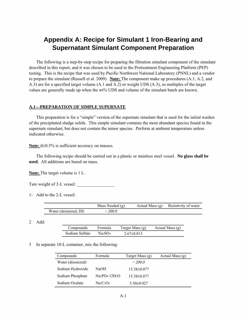
A.1
Appendix A: Recipe for Simulant 1 Iron-Bearing and Supernatant Simulant Component Preparation
The following is a step-by-step recipe for preparing the filtration simulant component of the simulant described in this report, and it was chosen to be used in the Pretreatment Engineering Platform (PEP) testing. This is the recipe that was used by Pacific Northwest National Laboratory (PNNL) and a vendor to prepare the simulant (Russell et al. 2009). Note: The component make up procedures (A.1, A.2, and A.3) are for a specified target volume (A.1 and A.2) or weight UDS (A.3), so multiples of the target values are generally made up when the wt% UDS and volume of the simulant batch are known. A.1—PREPARATION OF SIMPLE SUPERNATE
This preparation is for a “simple” version of the supernate simulant that is used for the initial washes of the precipitated sludge solids. This simple simulant contains the most abundant species found in the supernate simulant, but does not contain the minor species. Perform at ambient temperature unless indicated otherwise. Note: ≤0.5% is sufficient accuracy on masses.
The following recipe should be carried out in a plastic or stainless steel vessel. No glass shall be used. All additions are based on mass. Note: The target volume is 1 L. Tare weight of 2-L vessel: _________________ 1- Add to the 2-L vessel:
Mass Needed (g) Actual Mass (g) Resistivity of water
Water (deionized, DI) ~ 200.0 2 Add:
Compounds Formula Target Mass (g) Actual Mass (g) Sodium Sulfate Na2SO4 2.670.013
3 In separate 10-L container, mix the following:
Compounds Formula Target Mass (g) Actual Mass (g)
Water (deionized) ~ 200.0
Sodium Hydroxide NaOH 15.380.077
Sodium Phosphate Na3PO4·12H2O 15.380.077
Sodium Oxalate Na2C2O4 5.300.027

A.2
4 Mix vigorously for ~15 minutes. Then add the above solution to the 2-L vessel. 5 Add to the 2-L vessel:
Compounds Formula Target Mass (g) Actual Mass (g) Sodium Carbonate Na2CO3 102.30.51
6 Mix vigorously for ~15 minutes. 7 In separate 250-mL container, mix the following:
Compounds Formula Target Mass (g) Actual Mass (g)
Sodium Nitrite NaNO2 6.490.032
Water (deionized) ~ 100
8 Add to the 2-L vessel and mix vigorously for ~15 minutes. 9 Add to the 2-L vessel: Total Mass Target (g) Added Mass of Water to Add (g) DI Water to a total mass of: 1000 ~350 Record Final Mass of Vessel + solution: _________________ Record Final Mass of solution: _________________
A.2—PREPARATION OF SUPERNATE SIMULANT
This simulant is used for final washing of the Precipitated Sludge Solids and for makeup of the final overall simulant. Note: ≤0.5% is sufficient accuracy on masses.
The following recipe should be carried out in a plastic or stainless steel vessel. No glass shall be used. All additions are based on mass. Note: The target volume is 1 L. Tare weight of 2-L vessel: _________________ 1- To a 2-L vessel, add:
Target Mass (g) Actual Mass (g) Resistivity of water
Water (deionized, DI) ~ 200.0
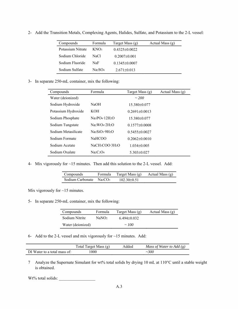
A.3
2- Add the Transition Metals, Complexing Agents, Halides, Sulfate, and Potassium to the 2-L vessel:
Compounds Formula Target Mass (g) Actual Mass (g)
Potassium Nitrate KNO3 0.43250.0022
Sodium Chloride NaCl 0.20070.001
Sodium Fluoride NaF 0.13450.0007
Sodium Sulfate Na2SO4 2.6710.013
3- In separate 250-mL container, mix the following:
Compounds Formula Target Mass (g) Actual Mass (g)
Water (deionized) ~ 200
Sodium Hydroxide NaOH 15.3800.077
Potassium Hydroxide KOH 0.26910.0013
Sodium Phosphate Na3PO4·12H2O 15.3800.077
Sodium Tungstate Na2WO4·2H2O 0.15770.0008
Sodium Metasilicate Na2SiO3·9H2O 0.54550.0027
Sodium Formate NaHCOO 0.20620.0010
Sodium Acetate NaCH3COO·3H2O 1.0340.005
Sodium Oxalate Na2C2O4 5.3030.027
4- Mix vigorously for ~15 minutes. Then add this solution to the 2-L vessel. Add:
Compounds Formula Target Mass (g) Actual Mass (g) Sodium Carbonate Na2CO3 102.300.51
Mix vigorously for ~15 minutes. 5- In separate 250-mL container, mix the following:
Compounds Formula Target Mass (g) Actual Mass (g)
Sodium Nitrite NaNO2 6.4940.032
Water (deionized) ~ 100
6- Add to the 2-L vessel and mix vigorously for ~15 minutes. Add:
Total Target Mass (g) Added Mass of Water to Add (g) DI Water to a total mass of: 1000 ~300 7 Analyze the Supernate Simulant for wt% total solids by drying 10 mL at 110°C until a stable weight
is obtained. Wt% total solids: _________________
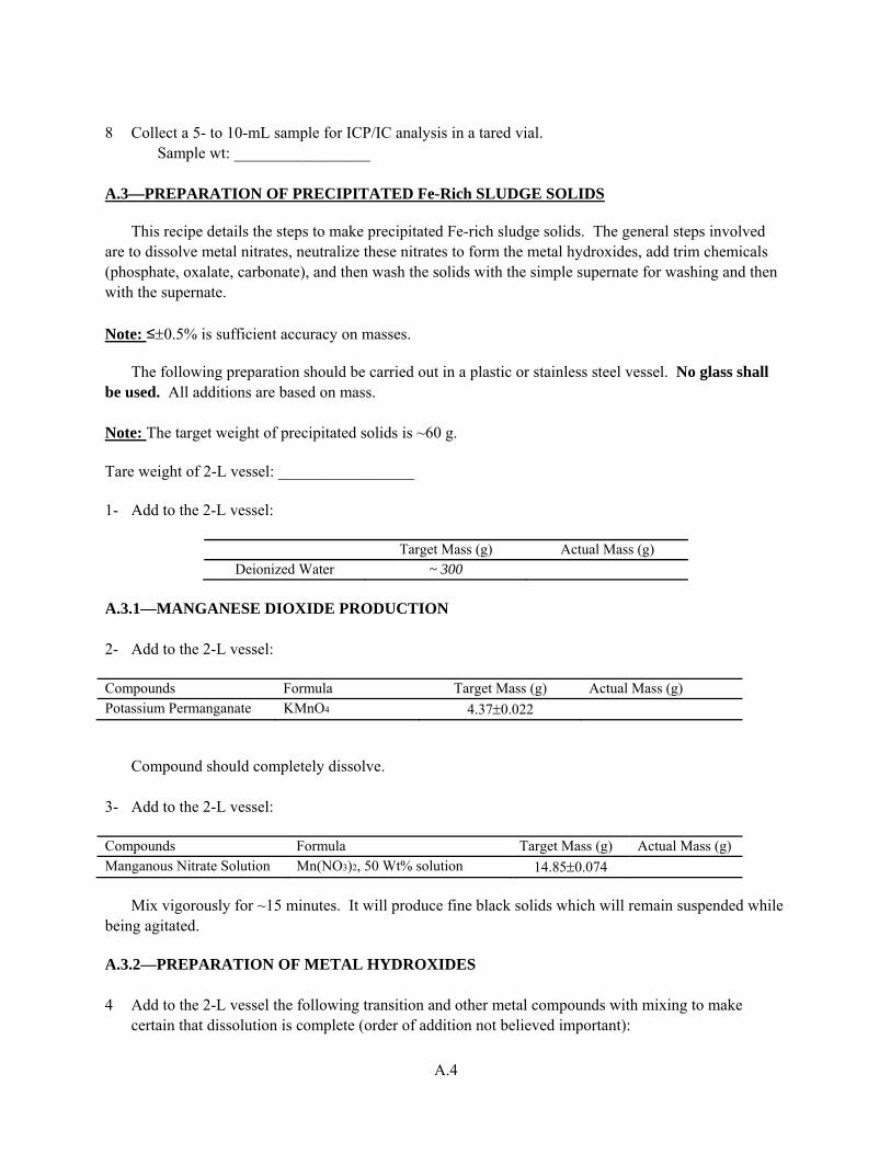
A.4
8 Collect a 5- to 10-mL sample for ICP/IC analysis in a tared vial. Sample wt: _________________ A.3—PREPARATION OF PRECIPITATED Fe-Rich SLUDGE SOLIDS
This recipe details the steps to make precipitated Fe-rich sludge solids. The general steps involved are to dissolve metal nitrates, neutralize these nitrates to form the metal hydroxides, add trim chemicals (phosphate, oxalate, carbonate), and then wash the solids with the simple supernate for washing and then with the supernate. Note: ≤0.5% is sufficient accuracy on masses.
The following preparation should be carried out in a plastic or stainless steel vessel. No glass shall be used. All additions are based on mass. Note: The target weight of precipitated solids is ~60 g. Tare weight of 2-L vessel: _________________ 1- Add to the 2-L vessel:
Target Mass (g) Actual Mass (g)
Deionized Water ~ 300 A.3.1—MANGANESE DIOXIDE PRODUCTION 2- Add to the 2-L vessel:
Compounds Formula Target Mass (g) Actual Mass (g) Potassium Permanganate KMnO4 4.370.022
Compound should completely dissolve. 3- Add to the 2-L vessel:
Compounds Formula Target Mass (g) Actual Mass (g) Manganous Nitrate Solution Mn(NO3)2, 50 Wt% solution 14.850.074
Mix vigorously for ~15 minutes. It will produce fine black solids which will remain suspended while being agitated. A.3.2—PREPARATION OF METAL HYDROXIDES 4 Add to the 2-L vessel the following transition and other metal compounds with mixing to make
certain that dissolution is complete (order of addition not believed important):
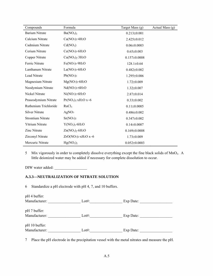
A.5
Compounds Formula Target Mass (g) Actual Mass (g)
Barium Nitrate Ba(NO3)2 0.2130.001
Calcium Nitrate Ca(NO3)2·4H2O 2.4250.012
Cadmium Nitrate Cd(NO3) 0.060.0003
Cerium Nitrate Ce(NO3)3·6H2O 0.650.003
Copper Nitrate Cu(NO3)2·3H2O 0.1570.0008
Ferric Nitrate Fe(NO3)3·9H2O 128.10.64
Lanthanum Nitrate La(NO3)3·6H2O 0.4820.002
Lead Nitrate Pb(NO3)2 1.2950.006
Magnesium Nitrate Mg(NO3)2·6H2O 1.720.009
Neodymium Nitrate Nd(NO3)3·6H2O 1.320.007
Nickel Nitrate Ni(NO3)2·6H2O 2.870.014
Praseodymium Nitrate Pr(NO3)3·xH2O x~6 0.330.002
Ruthenium Trichloride RuCl3 0.110.0005
Silver Nitrate AgNO3 0.4860.002
Strontium Nitrate Sr(NO3)2 0.3470.002
Yttrium Nitrate Y(NO3)3·6H2O 0.140.0007
Zinc Nitrate Zn(NO3)2·6H2O 0.1690.0008
Zirconyl Nitrate ZrO(NO3)2·xH2O x~6 1.730.009
Mercuric Nitrate Hg(NO3)2 0.0520.0003
5 Mix vigorously in order to completely dissolve everything except the fine black solids of MnO2. A
little deionized water may be added if necessary for complete dissolution to occur. DIW water added: _________________ A.3.3—NEUTRALIZATION OF NITRATE SOLUTION 6 Standardize a pH electrode with pH 4, 7, and 10 buffers. pH 4 buffer: Manufacturer: _________________ Lot#:_________________ Exp Date: _________________ pH 7 buffer: Manufacturer: _________________ Lot#:_________________ Exp Date: _________________ pH 10 buffer: Manufacturer: _________________ Lot#:_________________ Exp Date: _________________ 7 Place the pH electrode in the precipitation vessel with the metal nitrates and measure the pH.
A.6
pH: _________________ Note: pH should be <1.
With the nitrate solution agitating, slowly add 8-M NaOH until the pH reaches 10 to 11. Estimated amount of 8-M NaOH needed is 190 g. 8 Measure the pH. pH: _________________ 9 Continue mixing for 1 hour and then recheck pH. pH: _________________ 10 Add additional 8 M NaOH to return the pH to 10 if it is lower. Total 8M NaOH added: _________________ Final pH: _________________ A.3.4—ADDITION OF ADDITIONAL REAGENTS 11 Add to the 2-L vessel: Compounds Formula Target Mass (g) Actual Mass (g)
Calcium Fluoride CaF2 0.2050.001
Sodium Phosphate Na3PO4·12H2O 5.050.03
12 Combine the following in a separate 250-mL container while stirring: Compound Formula Target Mass (g) Actual Mass (g)
Water (deionized) ~ 100
Sodium Oxalate Na2C2O4 6.70.03
Add this sodium oxalate solution to the 2-L vessel while stirring. 13 Combine the following in a separate 250-mL container while stirring: Compound Formula Target Mass (g) Actual Mass (g)
Water (deionized) ~100
Sodium Carbonate Na2CO3 9.500.05
Add this sodium carbonate solution to the 2-L vessel with stirring. Approximate volume at this point should be about 0.9 L. 14 Mix (vigorously) the slurry to ensure good mixing. Mix the slurry for at least 1 hour.
A.7
A.3.5—WASH PRECIPITATED SLUDGE SOLIDS TO REMOVE NITRATE
Four washes are performed to reduce the nitrate concentration to below about 500 mg/kg. The slurry is centrifuged between each wash. The total solids content of the centrifuged solids needs to be at least 25 wt% for sufficient washing to be completed in four washes. If less wash solution is removed during centrifuging, additional washing steps must be added. However, excessive washing is to be avoided so that the nitrate and trace compounds are not reduced in concentration too far.
The amount of wash solution required per wash is approximately 3 times the mass of the centrifuged solids. Three washes with the “simple supernate for washing” are used, followed by a wash with the actual “supernate simulant.” Use this information to calculate the amount of wash and supernate simulant needed. 15 Centrifuge the slurry for 30 minutes at ~4500 G. Time started: _________________ Time finished: _________________ Centrifuge speed: _________________ 16 Decant the supernate. (The supernate is waste.) Amount of supernate decanted: _________________ 17 Combine all centrifuged slurry fractions. Weight of centrifuged solids: _________________ 18 Measure the nitrate concentration of the slurry using the nitrate probe for indication. NO3
- concentration: _________________ 19 Add “AY-102 simple simulant for washing” at approximately 3 times the mass of the slurry and mix
thoroughly (for ~1 hour). Amount of wash solution added: _________________ 20 Centrifuge the slurry for 30 minutes at ~4500 G. Time started: _________________ Time finished: _________________ Centrifuge speed: _________________ 21 Decant the supernate. (The supernate is waste.) End of Wash 1 Amount of supernate decanted: _________________ 22 Combine all centrifuged slurry fractions.
A.8
Weight of centrifuged solids: _________________ 23 Measure the nitrate concentration of the slurry using the nitrate probe for indication. NO3
- concentration: _________________ 24 Add “AY-102 simple simulant for washing” at approximately 3 times the mass of the slurry and mix
thoroughly (for ~1 hour). Amount of wash solution added: _________________ 25 Centrifuge the slurry for 30 minutes at ~4500 G. Time started: _________________ Time finished: _________________ Centrifuge speed: _________________ 26 Decant the supernate. (The supernate is waste.) End of Wash 2 Amount of supernate decanted: _________________ 27 Combine all centrifuged slurry fractions.
Weight of centrifuged solids: _________________ 28 Measure the nitrate concentration of the slurry using the nitrate probe for indication. NO3
- concentration: _________________ 29 Add “AY-102 simple simulant for washing” at approximately 3 times the mass of the slurry and mix
thoroughly (for ~1 hour). Amount of wash solution added: _________________ 30 Centrifuge the slurry for 30 minutes at ~4500 G. Time started: _________________ Time finished: _________________ Centrifuge speed: _________________ 31 Decant the supernate. (The supernate is waste.) End of Wash 3 Amount of supernate decanted: _________________ 32 Combine all centrifuged slurry fractions.
Weight of centrifuged solids: _________________

A.9
33 Measure the nitrate concentration of the slurry using the nitrate probe for indication. NO3
- concentration: _________________ 34 Add ACTUAL supernate simulant (the batch to be used for the final combined simulant) at
approximately 3 times the mass of the slurry and mix thoroughly (for ~1 hour). Amount of wash solution added: _________________ 35 Centrifuge the slurry for 30 minutes at ~4500 G. Time started: _________________ Time finished: _________________ Centrifuge speed: _________________ 36 Decant the supernate. (The supernate is waste.) End of Wash 4 Amount of supernate decanted: _________________ 37 Combine all centrifuged slurry fractions. Weight of centrifuged solids: _________________ 38 Measure the nitrate concentration of the slurry using the nitrate probe for indication. NO3
- concentration: _________________ 39 Add ACTUAL supernate simulant (the batch to be used for the final combined simulant) at
approximately 3 times the mass of the slurry and mix thoroughly (for ~1 hour). Amount of wash solution added: _________________ 40 Add to the 2-L vessel with agitation: Compounds Formula Target Mass (g) Actual Mass (g) Sodium Carbonate Na2CO3 156.00.78
41 Centrifuge the slurry for 30 minutes at ~4500 G. Time started: _________________ Time finished: _________________ Centrifuge speed: _________________ 42 Decant the supernate. (The supernate is waste.) End of Wash 5 Amount of supernate decanted: _________________
A.10
43 Measure the nitrate concentration of the slurry using the nitrate probe for indication. If <500 mg/kg, continue to next step. If not, then perform another washing step.
NO3
- concentration: _________________ 44 Analyze the slurry for wt% total solids and wt% supernate solids (wt% solids of supernate separated
from the slurry) by drying at 110°C. Wt% total solids: _________________ Wt% supernate solids: _________________ Acceptance Criteria
The acceptance criteria below apply to the PEP simulant. This is a good example of the criteria that might be required of a simulant vendor. These criteria are chosen to control the important features of the simulant, which are based on the application of the simulant. Hence, for another simulant, there could be an adjusted set of criteria that reflects another application.
Specific Supernate (i.e., Step 7 of Section A.2)
Shall be 5.0 0.5 M sodium, e.g., 5.0 10% (0.5M Na)
Anion concentrations in final supernate shall be 10% of target calculated from amounts added and final volume.
Fe-rich Solids Slurry (Step 14 of Section A.3)
Concentrations in the liquid phase of the slurry shall match the specific supernate acceptance criteria within 10% in all categories or as determined by the technical administrator.
The mass ratio of iron to other elements in the UDS shall be as given in Table A.1 within 10% for the elements whose mass ratio to iron is greater than 0.01 and within 20% for the elements whose mass ratio to iron is less than 0.01 or as determined by the technical administrator. Because of the very, very low solubility of zirconium, phosphate analysis of Zr is difficult in this high-phosphate medium, and it might not be observed without sophisticated analytical methods; we have successfully observed 80% of added Zr for this material.
Simulant (as shipped, not including the specific supernate set aside for rinsing)
Shall contain ≥ 5.8 wt% UDS.
Liquid phase shall be 5.00.5 M Na.
Concentrations in the liquid phase of the slurry (as defined at the beginning of Section 4) shall match the specific supernate acceptance criteria within 10% in all categories.
The mass ratio of iron to other elements in the simulant slurry shall be as given in Table A.1 within 10% for the elements whose mass ratio to iron is greater than 0.01 and within 20% for the elements whose mass ratio to iron is less than 0.01. Because of the very, very low solubility of zirconium, phosphate analysis of Zr is difficult in this high-phosphate medium, and it might not be observed without sophisticated analytical methods; we have successfully observed 80% of added Zr for this material.
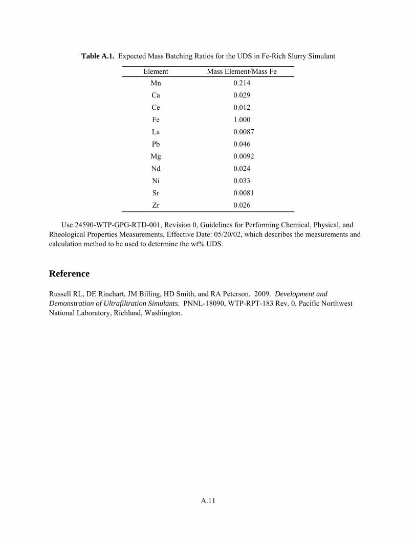
A.11
Table A.1. Expected Mass Batching Ratios for the UDS in Fe-Rich Slurry Simulant
Element Mass Element/Mass Fe
Mn 0.214
Ca 0.029
Ce 0.012
Fe 1.000
La 0.0087
Pb 0.046
Mg 0.0092
Nd 0.024
Ni 0.033
Sr 0.0081
Zr 0.026
Use 24590-WTP-GPG-RTD-001, Revision 0, Guidelines for Performing Chemical, Physical, and Rheological Properties Measurements, Effective Date: 05/20/02, which describes the measurements and calculation method to be used to determine the wt% UDS.
Reference Russell RL, DE Rinehart, JM Billing, HD Smith, and RA Peterson. 2009. Development and Demonstration of Ultrafiltration Simulants. PNNL-18090, WTP-RPT-183 Rev. 0, Pacific Northwest National Laboratory, Richland, Washington.

Appendix B
Simulant 1 Preparation

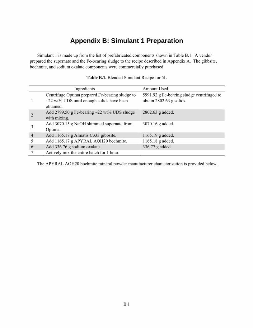
B.1
Appendix B: Simulant 1 Preparation
Simulant 1 is made up from the list of prefabricated components shown in Table B.1. A vendor prepared the supernate and the Fe-bearing sludge to the recipe described in Appendix A. The gibbsite, boehmite, and sodium oxalate components were commercially purchased.
Table B.1. Blended Simulant Recipe for 5L
Ingredients Amount Used
1 Centrifuge Optima prepared Fe-bearing sludge to ~22 wt% UDS until enough solids have been obtained.
5991.92 g Fe-bearing sludge centrifuged to obtain 2802.63 g solids.
2 Add 2799.50 g Fe-bearing ~22 wt% UDS sludge with mixing.
2802.63 g added.
3 Add 3070.15 g NaOH shimmed supernate from Optima.
3070.16 g added.
4 Add 1165.17 g Almatis C333 gibbsite. 1165.19 g added. 5 Add 1165.17 g APYRAL AOH20 boehmite. 1165.18 g added. 6 Add 336.76 g sodium oxalate. 336.77 g added. 7 Actively mix the entire batch for 1 hour.
The APYRAL AOH20 boehmite mineral powder manufacturer characterization is provided below.

B.2
The Almatis C333 gibbsite mineral powder manufacturer characterization is provided below.
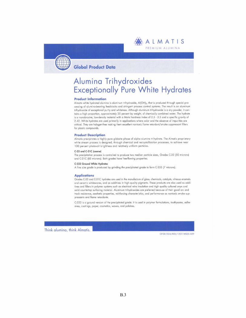
B.3
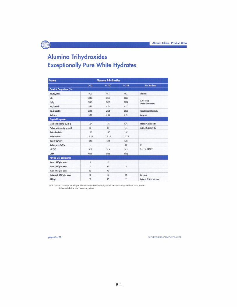
B.4
Appendix C
Recipe for Simulant 2 Preparation


C.1
Appendix C: Recipe for Simulant 2 Preparation
The following is a step-by-step recipe for preparing the simulant for the tank combination of tanks AN-101, C-104, C-111, and C-112. Note: The component make-up procedures are for a specified target volume or weight UDS, so multiples of the target values are generally made up when the wt% UDS and the volume of the simulant batch are known. The simulant had many of the minor waste components left out to lower the toxicity of the resultant simulant and make it easier to dispose of. C.1—PREPARATION OF PRECIPITATED SLUDGE SOLIDS
This recipe details the steps to make the precipitated sludge solids portion of the simulant. The general steps involved are to dissolve metal nitrates, neutralize these nitrates to form the metal hydroxides, add trim chemicals (phosphate, oxalate, carbonate), and then wash the solids with the simple supernate for washing and then with the supernate.
An accuracy of 0.5% on masses and volumes is sufficient.
The following preparation should be carried out in a plastic or stainless steel vessel. No glass shall be used. All additions are based on mass. Tare weight of 20-L vessel: _________________ 4- Add to the 20-L vessel:
Mass Needed (g) Actual Mass (g)
Deionized Water ~ 6000 5- Add to the 20-L vessel:
Compounds Formula Mass Needed (g) Actual Mass (g) Manganous Nitrate Solution Mn(NO3)2, 50 Wt % solution 255.33
Mix thoroughly. C.1.1—PREPARATION OF METAL HYDROXIDES 3- Add to the 20-L vessel the following transition and other metal compounds with mixing to make certain that dissolution is complete:
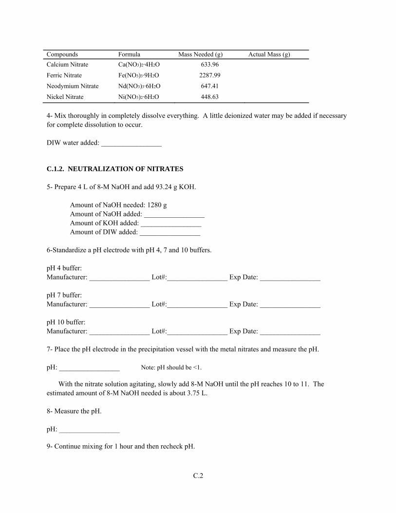
C.2
Compounds Formula Mass Needed (g) Actual Mass (g)
Calcium Nitrate Ca(NO3)2·4H2O 633.96
Ferric Nitrate Fe(NO3)3·9H2O 2287.99
Neodymium Nitrate Nd(NO3)3·6H2O 647.41
Nickel Nitrate Ni(NO3)2·6H2O 448.63
4- Mix thoroughly in completely dissolve everything. A little deionized water may be added if necessary for complete dissolution to occur. DIW water added: _________________ C.1.2. NEUTRALIZATION OF NITRATES 5- Prepare 4 L of 8-M NaOH and add 93.24 g KOH. Amount of NaOH needed: 1280 g
Amount of NaOH added: _________________ Amount of KOH added: _________________ Amount of DIW added: _________________ 6-Standardize a pH electrode with pH 4, 7 and 10 buffers. pH 4 buffer: Manufacturer: _________________ Lot#:_________________ Exp Date: _________________ pH 7 buffer: Manufacturer: _________________ Lot#:_________________ Exp Date: _________________ pH 10 buffer: Manufacturer: _________________ Lot#:_________________ Exp Date: _________________ 7- Place the pH electrode in the precipitation vessel with the metal nitrates and measure the pH. pH: _________________ Note: pH should be <1.
With the nitrate solution agitating, slowly add 8-M NaOH until the pH reaches 10 to 11. The estimated amount of 8-M NaOH needed is about 3.75 L. 8- Measure the pH. pH: _________________ 9- Continue mixing for 1 hour and then recheck pH.
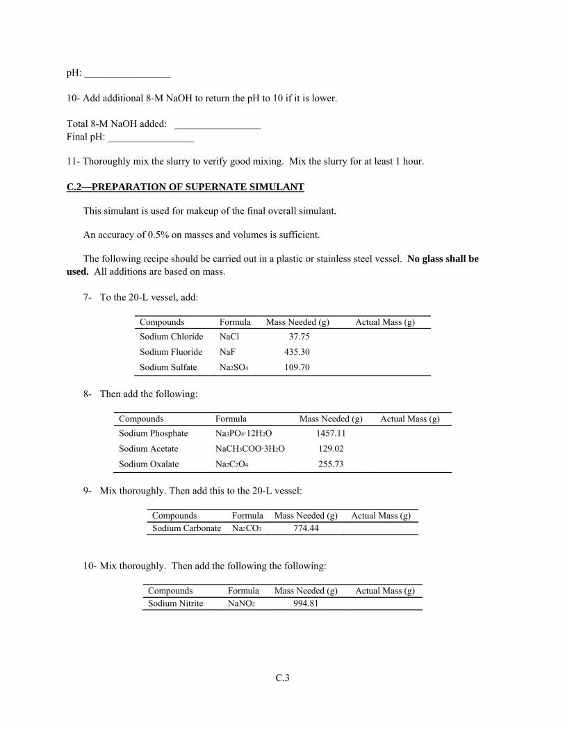
C.3
pH: _________________ 10- Add additional 8-M NaOH to return the pH to 10 if it is lower. Total 8-M NaOH added: _________________ Final pH: _________________ 11- Thoroughly mix the slurry to verify good mixing. Mix the slurry for at least 1 hour. C.2—PREPARATION OF SUPERNATE SIMULANT
This simulant is used for makeup of the final overall simulant.
An accuracy of 0.5% on masses and volumes is sufficient.
The following recipe should be carried out in a plastic or stainless steel vessel. No glass shall be used. All additions are based on mass.
7- To the 20-L vessel, add:
Compounds Formula Mass Needed (g) Actual Mass (g)
Sodium Chloride NaCl 37.75
Sodium Fluoride NaF 435.30
Sodium Sulfate Na2SO4 109.70
8- Then add the following:
Compounds Formula Mass Needed (g) Actual Mass (g)
Sodium Phosphate Na3PO4·12H2O 1457.11
Sodium Acetate NaCH3COO·3H2O 129.02
Sodium Oxalate Na2C2O4 255.73
9- Mix thoroughly. Then add this to the 20-L vessel:
Compounds Formula Mass Needed (g) Actual Mass (g) Sodium Carbonate Na2CO3 774.44
10- Mix thoroughly. Then add the following the following:
Compounds Formula Mass Needed (g) Actual Mass (g) Sodium Nitrite NaNO2 994.81
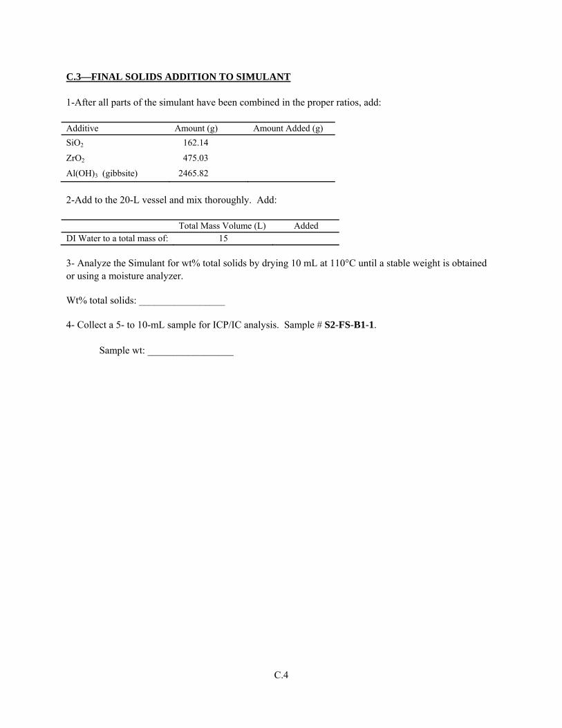
C.4
C.3—FINAL SOLIDS ADDITION TO SIMULANT 1-After all parts of the simulant have been combined in the proper ratios, add: Additive Amount (g) Amount Added (g)
SiO2 162.14
ZrO2 475.03
Al(OH)3 (gibbsite) 2465.82
2-Add to the 20-L vessel and mix thoroughly. Add:
Total Mass Volume (L) Added DI Water to a total mass of: 15 3- Analyze the Simulant for wt% total solids by drying 10 mL at 110°C until a stable weight is obtained or using a moisture analyzer. Wt% total solids: _________________ 4- Collect a 5- to 10-mL sample for ICP/IC analysis. Sample # S2-FS-B1-1. Sample wt: _________________
Appendix D
Simulant 2 Liquid Viscosity Flow Curves

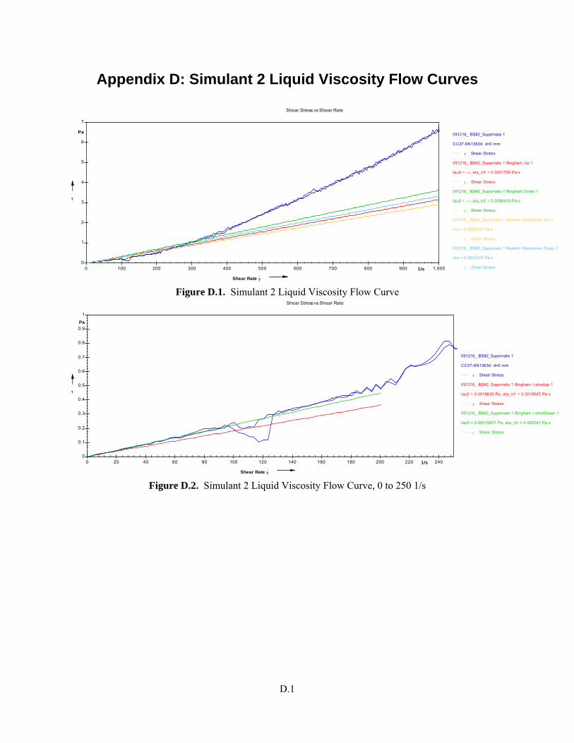
D.1
Appendix D: Simulant 2 Liquid Viscosity Flow Curves
0
1
2
3
4
5
6
7
Pa
0 100 200 300 400 500 600 700 800 900 1,0001/s
Shear Rate .
Shear Stress vs Shear Rate
091216_ BS#2_Supernate 1
CC27-SN13634; d=0 mm
Shear Stress
091216_ BS#2_Supernate 1 Bingham Up 1
tau0 = ---; eta_inf = 0.0031756 Pa·s
Shear Stress
091216_ BS#2_Supernate 1 Bingham Down 1
tau0 = ---; eta_inf = 0.0036415 Pa·s
Shear Stress
091216_ BS#2_Supernate 1 Newton INewtonian Up 1
eta = 0.0029142 Pa·s
Shear Stress
091216_ BS#2_Supernate 1 Newton INewtonian Down 1
eta = 0.0033219 Pa·s
Shear Stress
Figure D.1. Simulant 2 Liquid Viscosity Flow Curve
0
0.1
0.2
0.3
0.4
0.5
0.6
0.7
0.8
0.9
1
Pa
0 20 40 60 80 100 120 140 160 180 200 220 2401/s
Shear Rate .
Shear Stress vs Shear Rate
091216_ BS#2_Supernate 1
CC27-SN13634; d=0 mm
Shear Stress
091216_ BS#2_Supernate 1 Bingham I-shortup 1
tau0 = 0.0018639 Pa; eta_inf = 0.0018045 Pa·s
Shear Stress
091216_ BS#2_Supernate 1 Bingham I-shortDown 1
tau0 = 0.00015021 Pa; eta_inf = 0.002241 Pa·s
Shear Stress
Figure D.2. Simulant 2 Liquid Viscosity Flow Curve, 0 to 250 1/s

Appendix E
Simulant PSD Data

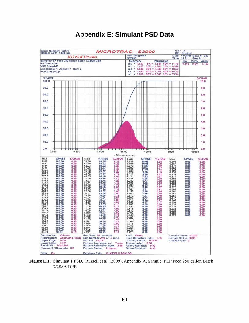
E.1
Appendix E: Simulant PSD Data
Figure E.1. Simulant 1 PSD. Russell et al. (2009), Appendix A, Sample: PEP Feed 250 gallon Batch
7/28/08 DER
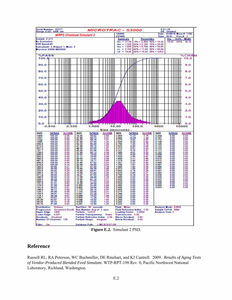
E.2
Figure E.2. Simulant 2 PSD.
Reference Russell RL, RA Peterson, WC Buchmiller, DE Rinehart, and KJ Cantrell. 2009. Results of Aging Tests of Vendor-Produced Blended Feed Simulant. WTP-RPT-198 Rev. 0, Pacific Northwest National Laboratory, Richland, Washington.
Appendix F
Simulant Slurry Rheology Flow Curves

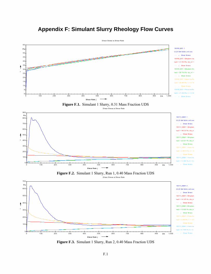
F.1
Appendix F: Simulant Slurry Rheology Flow Curves
0
5
1 0
1 5
2 0
2 5
3 0
3 5
4 0
4 5
5 0
6 0
P a
0 10 0 2 00 30 0 40 0 5 00 60 0 7 00 80 0 90 0 1,00 01 /s
Shea r Rate .
S he ar Stress vs Sh ea r Rate
100108_BS1 1
C C27-SN 13634; d=0 mm
Shear St res s
100108_BS1 1 B ingham Up
tau0 = 31.512 Pa; eta_in f =
Shear St res s
100108_BS1 1 B ingham Do
tau0 = 29.733 Pa; eta_in f =
Shear St res s
100108_BS1 1 Hersc hel-Bu
tau0 = 28.966 Pa; b = 0.158
Shear St res s
100108_BS1 1 Hersc hel-Bu
tau0 = 27.204 Pa; b = 0.156
Shear St res s
Figure F.1. Simulant 1 Slurry, 0.31 Mass Fraction UDS
0
10 0
20 0
30 0
40 0
50 0
60 0
70 0
80 0
90 0
P a
0 1 00 20 0 3 00 40 0 5 00 60 0 7 00 800 9 00 1,0 001 /s
S he ar Rate .
S hea r S tre ss vs She ar Ra te
100113_BS #1 1
CC 27-SN13634; d=0 mm
S hear St res s
100113_BS #1 1 Bingham
tau0 = 140.23 Pa; e ta_in f
S hear St res s
100113_BS #1 1 Bingham
tau0 = 20.431 Pa; e ta_in f
S hear St res s
100113_BS #1 1 Hers c he
tau0 = 4 ,823.5 P a; b = -4
S hear St res s
100113_BS #1 1 Hers c he
tau0 = 13.465 Pa; b = 0.6
S hear St res s
Figure F.2. Simulant 1 Slurry, Run 1, 0.40 Mass Fraction UDS
0
10 0
20 0
30 0
40 0
50 0
60 0
70 0
P a
0 1 00 20 0 3 00 40 0 5 00 60 0 7 00 800 9 00 1,0 001 /s
S he ar Rate .
S hea r S tre ss vs She ar Ra te
100113_BS #1 2
CC 27-SN13634; d=0 mm
S hear St res s
100113_BS #1 2 Bingham
tau0 = 141.87 Pa; e ta_in f
S hear St res s
100113_BS #1 2 Bingham
tau0 = 10.845 Pa; e ta_in f
S hear St res s
100113_BS #1 2 Hers c he
tau0 = 4 ,839 Pa; b = -4,4
S hear St res s
100113_BS #1 2 Hers c he
tau0 = 9 .1196 Pa; b = 0.1
S hear St res s
Figure F.3. Simulant 1 Slurry, Run 2, 0.40 Mass Fraction UDS
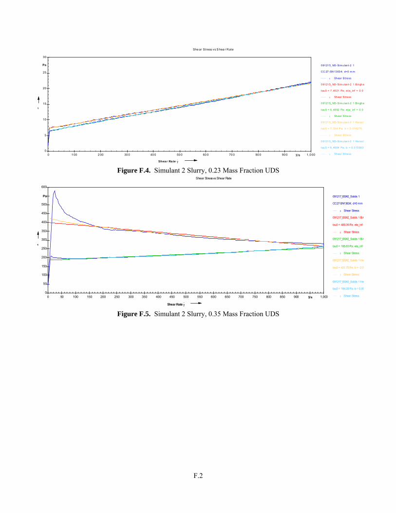
F.2
0
5
10
15
20
25
30
Pa
0 1 00 2 00 30 0 40 0 50 0 60 0 70 0 80 0 90 0 1,0 001/s
Shea r Ra te .
She ar Stress vs S hea r Rate
091215_M3-Simu lan t-2 1
CC 27-SN 13634; d=0 m m
Shear S tress
091215_M3-Simu lan t-2 1 Bingha
tau0 = 7 .4021 Pa; e ta_ inf = 0.01
Shear S tress
091215_M3-Simu lan t-2 1 Bingha
tau0 = 6 .4892 Pa; e ta_ inf = 0.01
Shear S tress
091215_M3-Simu lan t-2 1 Hersc h
tau0 = 7 .334 P a; b = 0 .016275; p
Shear S tress
091215_M3-Simu lan t-2 1 Hersc h
tau0 = 6 .4664 Pa; b = 0.015993 ;
Shear S tress
Figure F.4. Simulant 2 Slurry, 0.23 Mass Fraction UDS
0
50
100
150
200
250
300
350
400
450
500
600
Pa
0 50 100 150 200 250 300 350 400 450 500 550 600 650 700 750 800 850 900 1,0001/s
Shear Rate .
Shear Stress vs Shear Rate
091217_BS#2_Solids 1
CC27-SN13634; d=0 mm
Shear Stress
091217_BS#2_Solids 1 Bin
tau0 = 400.39 Pa; eta_inf =
Shear Stress
091217_BS#2_Solids 1 Bin
tau0 = 185.83 Pa; eta_inf =
Shear Stress
091217_BS#2_Solids 1 Her
tau0 = 431.75 Pa; b = -2.07
Shear Stress
091217_BS#2_Solids 1 Her
tau0 = 194.28 Pa; b = 0.00
Shear Stress
Figure F.5. Simulant 2 Slurry, 0.35 Mass Fraction UDS
PNNL-19250
Distr. 1
Distribution No. of Copies OFFSITE
No. of Copies ONSITE
13 Pacific Northwest National Laboratory G. N. Brown P7-25 W. C. Buchmiller K6-24 J. V. Crum K6-24 P. A. Gauglitz K7-15 E. C. Golovich K5-25 L. A. Mahoney K7-15 D. E. Rinehart K6-24 R. L. Russell K6-24 R. D. Scheele P7-25 B. E. Wells K7-15 Information Release (pdf)
3 WRPS N. W. Kirch R2-58 J. E. Meacham R2-58 D. J. Washenfelder R2-58


