handbook of financial markets: dynamics and evolution || complex evolutionary systems in behavioral...

CHAPTER 4

Complex Evolutionary Systemsin Behavioral Finance

Cars Hommes and Florian WagenerCeNDEF, School of Economics, University of Amsterdam

4.1. Introduction 2184.2. An Asset-Pricing Model with Heterogeneous Beliefs 221

4.2.1. The Fundamental Benchmark with Rational Agents 2224.2.2. Heterogeneous Beliefs 2234.2.3. Evolutionary Dynamics 2244.2.4. Forecasting Rules 225

4.3. Simple Examples 2264.3.1. Costly Fundamentalists vs. Trend Followers 2274.3.2. Fundamentalists vs. Opposite Biases 2294.3.3. Fundamentalists vs. Trend and Bias 2304.3.4. Efficiency 2304.3.5. Wealth Accumulation 2324.3.6. Extensions 236

4.4. Many Trader Types 2364.5. Empirical Validation 241

4.5.1. The Model in Price-to-Cash Flows 2424.5.2. Estimation of a Simple Two-Type Example 2464.5.3. Empirical Implications 251

4.6. Laboratory Experiments 2534.6.1. Learning to Forecast Experiments 2554.6.2. The Price-Generating Mechanism 2564.6.3. Benchmark Expectations Rules 2574.6.4. Aggregate Behavior 2594.6.5. Individual Prediction Strategies 2594.6.6. Profitability 262

4.7. Conclusion 264

Note: We would like to thank two anonymous references and the editor Klaus Reiner Schenk-Hoppe fordetailed comments on an earlier draft, which led to significant improvements. This research was supportedby the Netherlands Organization for Scientific Research (NWO) and by an EU STREP-grant “ComplexMarkets.”

HANDBOOK OF FINANCIAL MARKETS: DYNAMICS AND EVOLUTIONCopyright c© 2009, North-Holland, Elsevier, Inc. All rights reserved. 217

218 Chapter 4 • Complex Evolutionary Systems in Behavioral Finance

Appendix 4.1: Bifurcation Theory 266Appendix 4.2: Bifurcation Scenarios 268References 271

Abstract

Traditional finance is built on the rationality paradigm. This chapter discusses simplemodels from an alternative approach in which financial markets are viewed as complexevolutionary systems. Agents are boundedly rational and base their investment decisionson market-forecasting heuristics. Prices and beliefs about future prices co-evolve overtime with mutual feedback. Strategy choice is driven by evolutionary selection so thatagents tend to adopt strategies that were successful in the past. Calibration of “simplecomplexity models” with heterogeneous expectations to real financial market data andlaboratory experiments with human subjects are also discussed.

Keywords: stylized facts, power laws, agent-based models, interacting agents

4.1. INTRODUCTION

Finance is witnessing important changes, according to some even a paradigmatic shift,from the traditional, neoclassical mathematical modeling approach based on a rep-resentative, fully rational agent and perfectly efficient markets (Muth, 1961; Lucas,1971; Fama, 1970) to a behavioral approach based on computational models wheremarkets are viewed as complex evolving systems with many interacting, “boundedlyrational” agents using simple “rule of thumb” trading strategies (e.g., Anderson et al.,1988; Brock, 1993; Arthur, 1995; Arthur et al., 1997a; Tesfatsion and Judd, 2006).Investor’s psychology plays a key role in behavioral finance, and different types ofpsychology-based trading and behavioral modes have been identified in the literature,such as positive feedback or momentum trading, trend extrapolation, noise trading, over-confidence, overreaction, optimistic or pessimistic traders, upward- or downward-biasedtraders, correlated imperfect rational trades, overshooting, contrarian strategies, and soon. Some key references dealing with various aspects of investor psychology include,for example, Cutler et al. (1989), DeBondt and Thaler (1985), DeLong et al. (1990a,b),Brock and Hommes (1997, 1998), Gervais and Odean (2001), and Hong and Stein(1999, 2003), among others—see, for example, Shleifer (2000), Hirschleifer (2001),and Barberis and Thaler (2003) for extensive surveys and many more references onbehavioral finance.

An important problem of a behavioral approach is that it leaves “many degrees offreedom.” There are many ways individual agents can deviate from full rationality. Evo-lutionary selection based on relative performance is one plausible way to disciplinethe “wilderness of bounded rationality.” Milton Friedman (1953) argued that

Cars Hommes and Florian Wagener 219

nonrational agents will not survive evolutionary competition and will therefore be drivenout of the market, thus providing support to a representative rational agent frameworkas a (long run) description of the economy. In the same spirit, Alchian (1950) arguedthat biological evolution and natural selection driven by realized profits may elimi-nate nonrational, nonoptimizing firms and lead to a market in which rational, profitmaximizing firms dominate. Blume and Easley (1992, 2006) have, however, shownthat the market selection hypothesis does not always hold and that nonrational agentsmay survive in the market. Brock (1993, 1997), Arthur et al. (1997b), LeBaron et al.(1999), and Farmer (2002), among others, introduced artificial stock markets, describedby agent-based models with evolutionary selection between many different interactingtrading strategies. They showed that the market does not generally select for the ratio-nal, fundamental strategy and that simple technical trading strategies may survive inartificial markets. Computationally oriented agent-based simulation models have beenreviewed in LeBaron (2006); see also the special issue of the Journal of Mathemati-cal Economics (Hens and Schenk-Hoppe, 2005) and the survey chapter of Evstigneev,Hens, and Schenk-Hoppe (2009) in this book for an overview of evolutionaryfinance.1

Stimulated by work on artificial markets, in the last decade quite a number of “simplecomplexity models” have been introduced. Markets are viewed as evolutionary adaptivesystems with boundedly rational interacting agents, but the models are simple enough tobe at least partly analytically tractable. The study of simple complexity models typicallyrequires a well-balanced mixture of analytical and computational tools. This literatureis surveyed in Hommes (2006) and Chiarella et al. (2009); see also Lux (2009), whodiscusses in detail how well models with interacting agents match important stylizedfacts such as fat tails in the returns distribution and long memory. Without repeatingan extensive survey, this chapter focuses on a number of simple examples, in particularthe adaptive belief systems (ABSs) of Brock and Hommes (1997, 1998). These modelsserve as didactic examples of nonlinear dynamic asset-pricing models with evolutionarystrategy switching, and they illustrate some of the key features present in the interactingagents literature. The model also has been used to test the relevance of the theory of het-erogeneous expectations empirically as well as in laboratory experiments with humansubjects. Simple complexity models may also be used by practitioners or policy makers.To illustrate this point, we present an example showing how such a model can be usedto evaluate how likely it is that a stock market bubble will resume.

Two important features of the ABS are that agents are boundedly rational and thatthey have heterogeneous expectations. An ABS is in fact a standard discounted valueasset-pricing model derived from mean-variance maximization, extended to the caseof heterogeneous beliefs. Two classes of investors that are also observed in financialpractice can be distinguished: fundamentalists and technical analysts. Fundamentalistsbase their forecasts of future prices and returns on economic fundamentals, such asdividends, interest rates, price-earning ratios, and so on. In contrast, technical analystsare looking for patterns in past prices and base their forecasts upon extrapolation of

1Some other recent references are Amir et al. (2005) and Evstigneev et al. (2002, 2008).


these patterns. Fractions of these two types of traders are time varying and depend onrelative performance. Strategy choice is thus based on evolutionary selection or rein-forcement learning, with agents switching to more successful (i.e., profitable) rules.Asset price fluctuations are characterized by irregular switching between a stable phasewhen fundamentalists dominate the market and an unstable phase when trend followersdominate and asset prices deviate from benchmark fundamentals. Price deviations fromthe rational expectations fundamental benchmark and excess volatility are triggered bynews about economic fundamentals but may be amplified by evolutionary selection,based on recent performance, of trend-following strategies.

There is empirical evidence that experience-based reinforcement learning plays animportant role in investment decisions in real markets. For example, Ippolito (1992),Chevalier and Ellison (1997), Sirri and Tufano (1998), Rockinger (1996), and Karceski(2002) show for mutual funds data that money flows into past good performers whileflowing out of past poor performers and that performance persists on a short-term basis.Pension funds are less extreme in picking good performance but are tougher on badperformers (Del Guercio and Tkac, 2002). Benartzi and Thaler (2007) have shown thatheuristics and biases play a significant role in retirement savings decisions. For example,using data from Vanguard, they show that the equity allocation of new participants rosefrom 58% in 1992 to 74% in 2000, following a strong rise in stock prices in the late1990s; however, it dropped back to 54% in 2002, following the extreme fall in stockprices.

Laboratory experiments with human subjects have shown that individuals often donot behave fully rationally but tend to use heuristics, possibly biased, in making eco-nomic decisions under uncertainty (Kahneman and Tversky, 1973). In a similar vein,Smith et al. (1998) have shown the occurrence of bubbles and the ease with whichmarkets deviate from full rationality in asset-pricing laboratory experiments. Thesebubbles occur despite the fact that participants had sufficient information to computethe fundamental value of the asset. Laboratory experiments with human subjects pro-vide an important tool to investigate which behavioral rules play a significant role indeviations from the rational benchmark, and they can thus help discipline the class ofbehavioral modes. Duffy (2008) gives a stimulating recent overview concerning the roleof laboratory experiments to explain macro phenomena.

Heterogeneity in forecasting future asset prices is supported by evidence from sur-vey data. For example, Vissing-Jorgensen (2003) reports that at the beginning of 2000,50% of individual investors considered the stock market to be overvalued, approxi-mately 25% believed that it was fairly valued, about 15% were unsure, and less than10% believed that it was undervalued. This is an indication of heterogeneous beliefsamong individual investors about the prospect of the stock market. Similarly, Shiller(2000) finds evidence that investors’ sentiment varies over time. Both institutional andindividual investors become more optimistic in response to significant increases in therecent performance of the stock market.

This chapter is organized as follows. Section 4.2 introduces the main features ofadaptive belief systems, and Section 4.3 discusses a number of simple examples withtwo, three, and four different trader types. In Section 4.4 an analytical framework with


many different trader types is presented. Section 4.5 discusses the empirical relevanceof behavioral heterogeneity. The estimation of a simple model with fundamentalistsand chartists on yearly S&P 500 data shows how the worldwide stock market bubblein the late 1990s, triggered by good news about fundamentals (a new Internet tech-nology), may have been strongly amplified by trend-following strategies. Section 4.6reviews some learning to forecast laboratory experiments with human subjects, investi-gating which individual forecasting rules agents may use, how these rules interact, andwhich aggregate outcome they cocreate. Section 4.7 concludes the chapter, sketchingsome challenges for future research and potential applications for financial practitionersand policy makers. An appendix contains a short mathematical overview of bifurcationtheory, which plays a role in the transition to complicated price fluctuations in the simplecomplexity models discussed in this chapter.

4.2. AN ASSET-PRICING MODEL WITH HETEROGENEOUSBELIEFS

This section discusses the asset-pricing model with heterogeneous beliefs as introducedin Brock and Hommes (1998), using evolutionary selection of expectations as in Brockand Hommes (1997a). This simple modeling framework has been inspired by compu-tational work at the Santa Fe Institute (SFI) and may be viewed as a simple, partlyanalytically tractable version of the more complicated SFI artificial stock market ofArthur et al. (1997b).

Agents can invest in either a risk-free asset or a risky asset. The risk-free asset is inperfect elastic supply and pays a fixed rate of return r; the risky asset pays an uncer-tain dividend. Let pt be the price per share (ex-dividend) of the risky asset at time t,and let yt be the stochastic dividend process of the risky asset. Wealth dynamics isgiven by

Wt+1 = RWt + (pt+1 + yt+1 − Rpt)zt (4.1)

where R = 1 + r is the gross rate of risk-free return and zt denotes the number of sharesof the risky asset purchased at date t. Let Eht and Vht denote the “beliefs” or forecastsof trader type h about conditional expectation and conditional variance.

Agents are assumed to be myopic mean-variance maximizers so that the demand zhtof type h for the risky asset solves

Maxzt{Eht[Wt+1] − a

2Vht[Wt+1]} (4.2)

where a is the risk-aversion parameter. The demand zht for risky assets by trader type his then

zht =Eht[pt+1 + yt+1 − Rpt]aVht[pt+1 + yt+1 − Rpt]

=Eht[pt+1 + yt+1 − Rpt]

aσ2(4.3)


where the conditional variance Vht = σ2 is assumed to be constant and equal for alltypes.2 Let zs denote the supply of outside risky shares per investor, also assumed to beconstant, and let nht denote the fraction of type h at date t. Equilibrium of demand andsupply yields

H∑h=1

nhtEht[pt+1 + yt+1 − Rpt]

aσ2= zs (4.4)

where H is the number of different trader types.The forecasts Eht[pt+1 + yt+1] of tomorrow’s prices and dividends are made before

the equilibrium price pt has been revealed by the market and therefore will depend on apublically available information set It−1 = {pt−1, pt−2, . . .; yt−1, yt−2, . . .} of past pricesand dividends. Solving the heterogeneous market-clearing equation for the equilibriumprice gives

Rpt =H∑h= 1

nhtEht[pt+1 + yt+1] − aσ2zs (4.5)

The quantity aσ2zs may be interpreted as a risk premium for traders to hold risky assets.

4.2.1. The Fundamental Benchmark with Rational Agents

When all agents are identical and expectations are homogeneous, the equilibrium pricingEq. 4.5 reduces to

Rpt = Et[pt+1 + yt+1] − aσ2zs (4.6)

where Et is the common conditional expectation in the beginning of period t. It is wellknown that, assuming that a transversality condition limt→∞(Et[pt+k])/Rk = 0 holds,the price of the risky asset is given by the discounted sum of expected future dividendsminus the risk premium:

p∗t =∞∑k=1

Et[yt+k] − aσ2zs

Rk(4.7)

The price p∗t in Eq. 4.7 is called the fundamental rational expectations price, or thefundamental price for short. It is completely determined by economic fundamentals,which are here given by the stochastic dividend process yt. In this section we focus onthe case of an independently identically distributed (IID) dividend process yt, but theestimation of the simple two-type model discussed in Section 4.5 uses a nonstationarydividend process.3 For the special case of an IID dividend process yt, with constant

2Gaunersdorfer (2000) investigates the case with time-varying beliefs about variances and shows that the assetprice dynamics are quite similar. Chiarella and He (2002, 2003) investigate the model with heterogeneousrisk-aversion coefficients.3Brock and Hommes (1997b) also discuss a nonstationary example, in which the dividend process follows ageometric random walk.


mean E[yt] = y, the fundamental price is constant:

p∗ =∞∑k=1

y − aσ2zs

Rk=y − aσ2zs

r(4.8)

Recall that, in addition to the rational expectations fundamental solution in Eq. 4.7,so-called rational bubble solutions of the form pt = p∗t + (1 + r)t(p0 − p∗0) also satisfythe pricing Eq. 4.6. Along these bubble solutions, traders have rational expectations(perfect foresight), but they are ruled out by the transversality condition. In a perfectlyrational world, traders realize that such bubbles cannot last forever, and therefore alltraders believe that the value of a risky asset is always equal to its fundamental price.Changes in asset prices are then only driven by unexpected changes in dividends andrandom “news” about economic fundamentals. In a heterogeneous world the situationwill be quite different.

4.2.2. Heterogeneous Beliefs

It will be convenient to work with the deviation from the fundamental price

xt = pt − p∗t (4.9)

We make the following assumptions about the beliefs of trader type h:

B1 Vht[pt+1 + yt+1 − Rpt] = Vt[pt+1 + yt+1 − Rpt] = σ2, for all h, t.

B2 Eht[yt+1] = Et[yt+1] = y, for all h, t.

B3 All beliefs Eht[pt+1] are of the form

Eht[pt+1] = Et[p∗t+1] + Eht[xt+1] = p∗ + fh(xt−1, . . ., xt−L) (4.10)

for all h, t.According to B1, beliefs about conditional variance are equal and constant for all

types, as discussed already. Assumption B2 states that all types have correct expecta-tions about future dividends yt+1 given by the conditional expectation, which is y in thecase of IID dividends. According to B3, beliefs about future prices consist of two parts:a common belief about the fundamental plus a heterogeneous part fht.4 Each forecast-ing rule fh represents a model of the market (e.g., a technical trading rule) according towhich type h believes that prices will deviate from the fundamental price.

An important and convenient consequence of the assumptions B1–B3 about traders’beliefs is that the heterogeneous agent market equilibrium Eq. 4.5 can be reformulated indeviations from the benchmark fundamental. In particular, substituting the price forecast

4The assumption that all types know the fundamental price is without loss of generality, because any forecast-ing rule not using the fundamental price can be reparameterized or reformulated for mathematical conveniencein deviations from an (unknown) fundamental price p∗.


(Eq. 4.10) in the market equilibrium Eq. 4.5 and using Rp∗t = Et[p∗t+1 + yt+1] − aσ2zs

yields the equilibrium equation in deviations from the fundamental:

Rxt =H∑h=1

nhtEht[xt+1] ≡H∑h=1

nhtfht (4.11)

with fht = fh(xt−1, . . ., xt−L). Note that the benchmark fundamental is nested as a spe-cial case within this general setup, with all forecasting strategies fh ≡ 0. Hence, theadaptive belief systems can be used in empirical and experimental testing where assetprices deviate significantly from some benchmark fundamental.

4.2.3. Evolutionary Dynamics

The evolutionary part of the model describes how beliefs are updated over time, thatis, how the fractions nht of trader types evolve over time. These fractions are updatedaccording to an evolutionary fitness or performance measure. The fitness measures ofall trading strategies are publically available but subject to noise. Fitness is derived froma random utility model and given by

Uht = Uht + εiht (4.12)

where Uht is the deterministic part of the fitness measure and εiht represents anindividual agent’s IID error when perceiving the fitness of strategy h = 1, . . .H .

To obtain analytical expressions for the probabilities or fractions, the noise termεiht is assumed to be drawn from a double exponential distribution. As the number ofagents goes to infinity, the probability that an agent chooses strategy h is given by themultinomial logit model (or “Gibbs” probabilities):5

nht =eβUh,t−1∑Hh=1 e

βUh,t−1(4.13)

Note that the fractions nht add up to 1.A key feature of Eq. 4.13 is that the higher the fitness of trading strategy h, the

more traders will select strategy h. Hence, Eq. 4.13 represents a form of reinforcementlearning: Agents tend to switch to strategies that have performed well in the (recent)past. The parameter β in Eq. 4.13 is called the intensity of choice; it measures the sen-sitivity of the mass of traders to selecting the optimal prediction strategy. The intensityof choice β is inversely related to the variance of the noise terms εiht. The extreme caseβ = 0 corresponds to noise of infinite variance so that differences in fitness cannot beobserved and all fractions (4.13) will be fixed over time and equal to 1/H .

The other extreme case β = +∞ corresponds to the case without noise so that thedeterministic part of the fitness can be observed perfectly, and in each period, all traders

5See Manski and McFadden (1981) and Anderson, de Palma, and Thisse (1993) for extensive discussion ofdiscrete choice models and their applications in economics.


choose the optimal forecast. An increase in the intensity of choice β represents anincrease in the degree of rationality with respect to evolutionary selection of tradingstrategies. The timing of the coupling between the market equilibrium Eq. 4.5 or 4.11and the evolutionary selection of strategies (Eq. 4.13) is important. The market equilib-rium price pt in Eq. 4.5 depends on the fractions nht. The notation in Eq. 4.13 stressesthe fact that these fractions nht depend on most recently observed past fitnesses Uh,t−1,which in turn depend on past prices pt−1 and dividends yt−1 in periods t − 1 further inthe past, as shown next. After the equilibrium price pt has been revealed by the market,it will be used in evolutionary updating of beliefs and determining the new fractionsnh,t+1. These new fractions will then determine a new equilibrium price pt+1, and so on.In an adaptive belief system, market equilibrium prices and fractions of different tradingstrategies thus coevolve over time.

A natural candidate for evolutionary fitness is (a weighted average of) realizedprofits, given by6

Uht = (pt + yt − Rpt−1)Eh,t−1[pt + yt − Rpt−1]

aσ2+ wUh,t−1 (4.14)

where 0 ≤ w ≤ 1 is a memory parameter measuring how fast past realized fitness isdiscounted for strategy selection.

Fitness can be rewritten in terms of deviations from the fundamental as

Uht = (xt − Rxt−1 + aσ2zs + δt)(fh,t−1 − Rxt−1 + aσ2zs

aσ2

)+ wUh,t−1 (4.15)

where δt ≡ p∗t + yt − Et−1[p∗t + yt] is a martingale difference sequence.

4.2.4. Forecasting Rules

To complete the model, we have to specify the class of forecasting rules. Brock andHommes (1998) have investigated evolutionary competition between simple linearforecasting rules with only one lag, that is,

fht = ghxt−1 + bh (4.16)

It can be argued that, for a forecasting rule to have any impact in real markets, ithas to be simple, because it seems unlikely that enough traders will coordinate on a

6Note that this fitness measure does not take into account the risk taken at the moment of the investmentdecision. In fact, one could argue that the fitness measure (Eq. 4.14) does not take into account the varianceterm in (Eq. 4.2) capturing the investors’ risk taken before obtaining that profit. On the other hand, in realmarkets, realized net profits or accumulated wealth may be what investors care about most, and the non-risk adjusted fitness measure (Eq. 4.14) may thus be of relevance in practice. See also DeLong et al. (1990)for a discussion of this point. Given that investors are risk averse, mean-variance maximizers maximizingtheir expected utility from wealth (Eq. 4.2), an alternative natural candidate for fitness, the risk-adjustedprofit given by πht = Rtzh,t−1 − a

2σ2z2h,t−1, where Rt = pt + yt −Rpt−1 and zh,t−1 = Eh,t−1[Rt]/(aσ2) is

the demand by trader type h. Hommes (2001) shows that the risk-adjusted fitness measure is, up to atype-independent level, equivalent to minus-squared prediction errors.


complicated rule. The simple linear rule (Eq. 4.16) includes a number of importantspecial cases. For example, when both the trend and the bias parameters gh = bh = 0,the rule reduces to the fundamentalists forecast, that is,

fht ≡ 0 (4.17)

predicting that the deviation x from the fundamental will be 0, or equivalently, thatthe price will be at its fundamental value. Other important cases covered by the linearforecasting rule (Eq. 4.16) are the pure trend followers:

fht = ghxt−1 gh > 0 (4.18)

and the pure biased belief

fht = bh (4.19)

Notice that the simple pure bias forecast (Eq. 4.19) represents any positively ornegatively biased forecast of next period’s price that traders might have. Instead ofthese extremely simple habitual rule-of-thumb forecasting rules, some might prefer therational, perfect foresight forecasting rule:

fht = xt+1 (4.20)

We emphasize, however, that the perfect foresight forecasting rule (Eq. 4.20)assumes perfect knowledge of the heterogeneous market equilibrium Eq. 4.5, and inparticular perfect knowledge about the beliefs of all other traders. Although the casewith perfect foresight has much theoretical appeal, its practical relevance in a complexheterogeneous world should not be overstated, since this underlying assumption seemsrather strong.7

4.3. SIMPLE EXAMPLES

This section presents simple but typical examples of adaptive belief systems (ABSs),with two, three, or four competing linear forecasting rules (Eq. 4.16), where theparameter gh represents a perceived trend in prices and the parameter bh represents aperceived upward or downward bias. The ABS with H types is given by (in deviations

7Brock and Hommes (1997) analyze the cobweb model with costly rational versus cheap naıve expectationsand find irregular price fluctuations due to endogenous switching between free riding and costly rationalforecasting. In general, however, a temporary equilibrium model with heterogeneous beliefs, such as theasset-pricing model, is difficult to analyze if one of the types has perfect foresight. Brock et al. (2008) discusshow a perfect foresight trader may affect the dynamics in an asset-pricing model with heterogeneous beliefs.


from the fundamental benchmark):

(1 + r)xt =H∑h=1

nht(ghxt−1 + bh) + εt (4.21)

nh,t =eβUh,t−1∑Hh=1 e

βUh,t−1(4.22)

Uh,t−1 = (xt−1 − Rxt−2)(ghxt−3 + bh − Rxt−2

aσ2

)+ wUh,t−2 − Ch (4.23)

where εt is a small noise term representing, for example, a small fraction of noise tradersand/or random outside supply of the risky asset.

To keep the analysis of the dynamical behavior tractable, Brock and Hommes (1998)focused on the case where the memory parameter w = 0, so that evolutionary fitness isgiven by last period’s realized profit. A common feature of all examples is that, as theintensity of choice to switch prediction or trading strategies increases, the fundamentalsteady state becomes locally unstable and nonfundamental steady states, cycles, or evenchaos arise. In the examples that follow, we encounter different bifurcation routes (i.e.,transitions) to complicated dynamics. A mathematical appendix summarizes the mostimportant bifurcations, that is, qualitative changes in the dynamics (e.g., when a steadystate loses stability or a new cycle is created) when a model parameter changes.

4.3.1. Costly Fundamentalists vs. Trend Followers

The simplest example of an ABS only has two trader types, with forecasting rules

f1t = 0 fundamentalists (4.24)f2t = gxt−1 g > 0 trend followers (4.25)

The first type are fundamentalists predicting that the price will equal its fundamentalvalue (or equivalently that the deviation will be zero) and the second type are pure trendfollowers predicting that prices will rise (or fall) by a constant rate. In this example, thefundamentalists have to pay a fixed per-period positive cost C1 for information gather-ing; in all other examples discussed later, information costs are set to zero for all tradertypes.

For small values of the trend parameter 0 ≤ g < 1 + r, the fundamental steadystate is always stable. Only for sufficiently high trend parameters, g > 1 + r, trendfollowers can destabilize the system. For trend parameters 1 + r < g < (1 + r)2, thedynamic behavior of the evolutionary system depends on the intensity of choice toswitch between the two trading strategies.8 For low values of the intensity of choice,

8For g > (1 + r)2 the system may become globally unstable and prices may diverge to infinity. Imposing astabilizing force—for example, by assuming that trend followers condition their rule on deviations from thefundamental, as in Gaunersdorfer, Hommes, and Wagener (2008)—leads to a bounded system again, possiblywith cycles or even chaotic fluctuations.


2221.5

2120.5

00.5

11.5

22.5

0 50 100 150 2000

0.2

0.4

0.6

0.8

1

0 50 100 150 200

0

0.2

0.4

0.6

0.8

1

22 21 0 1 2

(a) (b)

(c)

FIGURE 4.1 Time series of price deviations from fundamental (a) and fractions of fundamentalists (b)and attractor (c) in the (xt, n1t)-phase space for two-type model with costly fundamentalist versus trendfollowers buffeted with small noise (SD = 0.1). Price dynamics are characterized by temporary bubbles whentrend followers dominate the market, interrupted by sudden crashes, when fundamentalists dominate. In thepresence of (small) noise, the system switches back and forth between two coexisting quasiperiodic attractorsof the underlying deterministic skeleton, one with prices above and one with prices below its fundamentalvalue. Parameters are β = 3.6, g = 1.2, R = 1.1, and C = 1.

the fundamental steady state will be stable. As the intensity of choice increases, thefundamental steady state becomes unstable due to a pitchfork bifurcation in which twoadditional nonfundamental steady states −x∗ < 0 < x∗ are created.

As the intensity of choice increases further, the two nonfundamental steady statesalso become unstable due to a Hopf bifurcation, and limit cycles or even strangeattractors can arise around each of the (unstable) nonfundamental steady states.9 Theevolutionary ABS may cycle around the positive nonfundamental steady state, cyclearound the negative nonfundamental steady state, or, driven by the noise, switch backand forth between cycles around the high and the low steady states, as illustrated inFigure 4.1. The simulations use the E&F Chaos software as discussed in Diks et al.(2008).

This example shows that, in the presence of information costs and with zero memory,when the intensity of choice in evolutionary switching is high, fundamentalists cannot

9See Appendix 4.2 for a more detailed discussion of the pitchfork bifurcation and the Hopf bifurcation.


21.522

2120.5

00.5

11.5

2

2 2.5 3 3.5 4

(a) (b)

20.1

20.08

20.06

20.04

20.02

0

0.02

0.04

2 2.5 3 3.5 4

FIGURE 4.2 Bifurcation diagram (a) and largest Lyapunov exponent plot (b) as a function of the inten-sity of choice β for two-type model with costly fundamentalist versus trend followers. In both plots the modelis buffeted with very small noise (SD = 10−6) for the noise term εt in Eq. 4.21; to avoid that for largeβ values the system gets stuck in the locally unstable steady state. Parameters are g = 1.2, R = 1.1, C = 1,and 2 ≤ β ≤ 4. A pitchfork bifurcation of the fundamental steady state, in which two stable nonfundamentalsteady states are created, occurs for β ≈ 2.37. The nonfundamental steady states become unstable due to aHopf bifurcation for β ≈ 3.33, and (quasi-)periodic dynamics arise. For large values of β the largest Lyapunovexponent becomes positive, indicating chaotic price dynamics.

drive out pure trend followers and persistent deviations from the fundamental price mayoccur.10

Figure 4.2 illustrates that the asset-pricing model with costly fundamentalists versuscheap trend-following exhibits a rational route to randomness, that is, a bifurcationroute to chaos occurs as the intensity of choice to switch strategies increases.

4.3.2. Fundamentalists vs. Opposite Biases

The second example of an ABS is an example with three trader types without anyinformation costs. The forecasting rules are

f1t = 0 fundamentalists (4.26)f2t = b b > 0, positive bias (optimists) (4.27)f3t = −b − b < 0 negative bias (pessimists) (4.28)

The first type are fundamentalists as before, but there are no information costs for funda-mentalists. The second and third types have a purely biased belief, expecting a constantprice above and below, respectively, the fundamental price.

For low values of the intensity of choice, the fundamental steady state is stable. Asthe intensity of choice increases the fundamental steady becomes unstable due to aHopf bifurcation and the dynamics of the ABS is characterized by cycles around the

10Brock and Hommes (1999) show that this result also holds when the memory in the fitness measureincreases. In fact, an increase in the memory of the evolutionary fitness leads to bifurcation routes very similarto bifurcation routes that are due to an increase in the intensity of choice.


unstable steady state. This example shows that, even when there are no informationcosts for fundamentalists, they cannot drive out other trader types with opposite biasedbeliefs. In the evolutionary ABS with high intensity of choice, fundamentalists andbiased traders coexist with fractions varying over time and prices fluctuating aroundthe unstable fundamental steady state.

Moreover, Brock and Hommes (1998, p. 1259, Lemma 9) show that as the intensityof choice tends to infinity the ABS converges to a (globally) stable cycle of Period 4.Average profits along this four-cycle are equal for all three trader types. Hence, ifthe initial wealth is equal for all three types, in this evolutionary system in the longrun, accumulated wealth will be equal for all three types. This example shows thatthe Friedman argument that smart fundamental traders will always drive out simplerule-of-thumb speculative traders is in general not valid.11

4.3.3. Fundamentalists vs. Trend and Bias

The third example of an ABS is an example with four trader types, with linear fore-casting rules (Eq. 4.16) with parameters g1 = 0, b1 = 0; g2 = 0.9, b2 = 0.2; g3 = 0.9,b3 = −0.2; and g4 = 1 + r = 1.01, b4 = 0. The first type are fundamentalists again,without information costs, and the other three types follow a simple linear forecastingrule with one lag. The dynamical behavior is illustrated in Figures 4.3 and 4.4.

For low values of the intensity of choice, the fundamental steady state is stable. Asthe intensity of choice increases, as in the previous three-type example, the fundamentalsteady becomes unstable due to a Hopf bifurcation and a stable invariant circle aroundthe unstable fundamental steady state arises, with periodic or quasi-periodic fluctua-tions. As the intensity of choice further increases, the invariant circle breaks into astrange attractor with chaotic fluctuations. In the evolutionary ABS, fundamentalistsand chartists coexist with time-varying fractions and prices moving chaotically aroundthe unstable fundamental steady state. Figure 4.4 shows that in this four-type exam-ple with fundamentalists versus trend followers and biased beliefs a rational route torandomness occurs, with positive largest Lyapunov exponents for large values of β.

This four-type example shows that, even when there are no information costs for fun-damentalists, they cannot drive out other simple trader types and fail to stabilize pricefluctuations toward its fundamental value. As in the three-type case, the opposite biasescreate cyclic behavior and trend extrapolation turns these cycles into unpredictablechaotic fluctuations.

4.3.4. Efficiency

What can be said about market efficiency in an ABS? The (noisy) chaotic pricefluctuations are characterized by an irregular switching between phases of close-to-the-fundamental-price fluctuations, phases of “optimism” with prices following an upward

11This result is related to DeLong et al. (1990a,b), who show that a constant fraction of noise traders cansurvive in the market in the presence of fully rational traders. The ABS, however, are evolutionary modelswith time-varying fractions, driven by strategy performance.


20.25 20.5

20.75

0.75

20.5 20.5

0.5

21

1

0

0.05

0.05

20.05

20.05

0.1

0.1

0

00.2520.750.75 0.5 0.750

0.5

20.25

0.25

0

20.75

0.75

20.5

0.5

20.25

0.25

0

100 200 300

(a)

400 500 100 200 300

(b)

(c) (d)

400 500

FIGURE 4.3 Chaotic (a) and noisy chaotic (b) time series of asset prices in an adaptive belief systemwith four trader types. Strange attractor (c) and enlargement of strange attractor (d). Belief parameters areg1 = 0, b1 = 0; g2 = 0.9, b2 = 0.2; g3 = 0.9, b3 = −0.2; and g4 = 1 + r = 1.01, b4 = 0. Other parameters arer = 0.01, β = 90.5, w = 0, and Ch = 0 for all 1 ≤ h ≤ 4.

20.8

20.6

20.4

20.2

0

0.2

0.4

0.6

0.8

20.1

20.05

0

0.05

0.1

40 50 60 70

(a) (b)

80 90 100 40 50 60 70 80 90 100

FIGURE 4.4 Bifurcation diagram (a) and largest Lyapunov exponent plot (b) for the four-type model,buffeted with very small noise (SD = 10−6 for noise term εt in Eq. 4.21) to avoid that for large β-values thesystem gets stuck in the locally unstable steady state. Belief parameters are g1 = 0, b1 = 0; g2 = 0.9, b2 = 0.2;g3 = 0.9, b3 = −0.2; and g4 = 1 + r = 1.01, b4 = 0. Other parameters are r = 0.01, β = 90.5, w = 0, andCh = 0 for all 1 ≤ h ≤ 4. The four-type model with fundamentalists versus trend followers and biased beliefsexhibits a Hopf bifurcation at β = 50. A rational route to randomness (i.e., a bifurcation route to chaos)occurs, with positive largest Lyapunov exponents, when the intensity of choice becomes large.


trend, and phases of “pessimism,” with (small) sudden market crashes, as illustratedin Figure 4.3. In fact, in the ABS, prices are characterized by evolutionary switchingbetween the fundamental value and temporary speculative bubbles. Prices deviate per-sistently from their fundamental value; therefore it can be said that prices are excessivelyvolatile. In this sense the market is inefficient. But are these deviations easy to predict?Even in the simple, stylized four-type example in the purely deterministic chaotic case,the timing and direction of the temporary bubbles seem hard to predict, but once a bub-ble has started, the collapse of the bubble seems predictable. In the presence of (small)noise, however, the situation is quite different, as illustrated in Figure 4.3 (top right):The timing, the direction and the collapse of the bubble all seem hard to predict.

To stress this point further, we investigate this (un)predictability by employing aso-called nearest neighbor forecasting method to predict the returns, at lags 1 to 20for the purely chaotic as well as for several noisy chaotic time series, as illustrated inFigure 4.5.12 Nearest-neighbor forecasting looks for patterns in the past that are close tothe most recent pattern and then predicts the average value following all nearby past pat-terns. According to Takens’ embedding theorem, this method yields good forecasts fordeterministic chaotic systems.13 Figure 4.5 shows that as the noise level increases, theforecasting performance of the nearest-neighbor method quickly deteriorates. There-fore, in our simple nonlinear evolutionary ABS with noise, it is hard to make goodforecasts of future returns and to predict when prices will return to fundamental value.Our simple nonlinear ABS with small noise thus captures some of the intrinsic unpre-dictability of asset returns also present in real markets, and in terms of predictability themarket is close to being efficient.

4.3.5. Wealth Accumulation

The evolutionary dynamics in an ABS are driven by realized short-run profits, andchartists strategies survive in a world driven by short-run profit opportunities. Inthis subsection, we briefly look at the accumulated wealth in an ABS. Recall thataccumulated wealth for strategy type h is given by

Wh,t+1 = RWht + (pt+1 + yt+1 − Rpt)zht (4.29)

The first term represents wealth growth due to the risk-free asset, while the last termrepresents wealth growth (or decay) due to investments in the risky asset. Because ofmarket clearing, the average net inflow of wealth due to investment in the risky asset isgiven by ∑

h

nhtzht(pt+1 + yt+1 − Rpt) = zs(pt+1 + yt+1 − Rpt) (4.30)

12We would like to thank Sebastiano Manzan for providing this figure.13See Kantz and Schreiber (1997) for an extensive treatment of nonlinear time-series analysis and forecastingtechniques.


0 2 4 6 8 10 12 14 16 18 200

0.2

0.4

0.6

0.8

1

Pre

dict

ion

erro

r

Prediction horizon

Chaos5% noise10%30%40%

FIGURE 4.5 Forecasting errors for nearest-neighbor method applied to chaotic and noisy chaotic returnsseries for different noise levels in the four-type adaptive belief system. All returns series have close to 0autocorrelations at all lags. The benchmark case of prediction by the mean 0 is represented by the horizontalline at the normalized prediction error 1. Nearest-neighbor forecasting applied to the purely deterministicchaotic series leads to much smaller forecasting errors at all prediction horizons, 1–20 (bottom graph). A noiselevel of, say, 10% means that the ratio of the variance of the noise εt and the variance of the deterministicprice series is 1/10. As the noise level increases, the graphs shift upward, indicating that prediction errorsincrease. Small dynamic noise thus quickly deteriorates forecasting performance.

This is the average risk premium required by the population of investors to hold therisky asset. In the special case zs = 0 the risk premium is 0 and on average wealth ofeach strategy grows at the risk-free rate.

Figure 4.6 shows the development of prices and wealth of each strategy in the three-type and four-type examples of Subsections 4.3.2 and 4.3.3. Prices fluctuate aroundthe fundamental price. For the three-type example, the wealth accumulated by each ofthe three strategies—fundamentalists, optimistic biased, and pessimistic biased—growsover time, at an equal rate. Recall that in the three-type example, for an infinite intensityof choice β, the system converges to a stable four-cycle with average profits equal forall three strategies. At each time t, profits of fundamentalists are always between prof-its of optimists and pessimists, but on average all profits are (almost) equal, and thusaccumulated wealth grows at the same rate.14

14For finite intensity of choice, for example, β = 3000 as in Figure 4.6, wealth of the three-types growsat almost the same rate. For initial states chosen, as in Figure 4.6, wealth of the optimistic types slightlydominates the other two types.


9.759.8

9.859.9

9.9510

10.0510.1

10.1510.2

0 10 20 30 40 500

0.5

1

1.5

2

0 5 10 15 20

8.5

9

9.5

10

10.5

11

11.5

12

0 50 100 150 200

9

9.5

10

10.5

11

0 50 100

(a)

150 200

22

0

2

4

6

8

10

12

0 20 40 60 80 100

(b)

2221

0 1 2 3 4 5 6 7

0 20 40 60 80 100

FIGURE 4.6 Time series of prices (a) and accumulated wealth (b) in three-type ABS (top), four-typeABS (middle), and five-type ABS (bottom). Belief parameters are b = 0.2 for the three-type ABS (see sub-section 4.3.2) and as in Figure 4.3 in the four-type case. Other parameters are β = 3000 and σε = 0.025(three-type ABS); g4 = (1 + r)2 = 1.0201, β = 180, y = 0.1, R = 1.01, σε = 0.2 (four-type ABS), andσε = 0.1; and threshold parameter ϑ = 0.5 for switching strategy (five-type ABS).

In the four-type example, trend-following strategies are profitable during temporarybubbles. Fundamentalists suffer losses during temporary bubbles, but these losses arelimited. When the bubble bursts, fundamentalists make large profits while trend fol-lowers suffer from huge losses. On average, accumulated wealth of fundamentalistsincreases while wealth of chartists decreases, as illustrated in Figure 4.6.


The wealth in Eq. 4.29 corresponds to the accumulated wealth of a trader who alwaysuses strategy h. How would a switching strategy perform in a heterogeneous market?Figure 4.6 (bottom panel) illustrates an example of an ABS with five strategies, wherea switching strategy has been added to the four-type ABS. The fifth switching strategyis endogenous in the five-type ABS and thus affects the realized market price in thesame way as the other four strategies. The switching strategy always picks the bestof the other four strategies, according to last period’s realized profits, conditional onhow far the price deviates from the fundamental benchmark. In the simulation, whenthe price deviation becomes larger than a threshold parameter (ϑ = 0.5), the switchingstrategy switches back to the fundamental strategy to avoid losses when the bubblecollapses.

Figure 4.6 (bottom row) illustrates two features of the five-type ABS. First, dueto the presence of the switching strategy, the amplitude of price fluctuations (bottomrow, left plot) is somewhat smaller than in the four-type ABS. This is caused by theswitching strategy switching back to the fundamental strategy when the price devia-tion exceeds the threshold. Second, the accumulated wealth of the switching strategyoutperforms all other strategies, including the fundamental strategy—see Figure 4.6,bottom row, right plot. Notice that the two best strategies, the switching strategy and thefundamental strategy, also require the most information. The trend-following strategiesonly use publically available information on past prices.15 The fundamental strategyuses fundamental information, whereas the switching strategy uses fundamental infor-mation as well as information about competing strategies in the market and theirperformance.

In the ABS evolutionary framework, agents switch strategies based on short-run real-ized profits. In the long run, a fundamental strategy often accumulates more wealth thantrend-following rules. However, fundamental strategies suffer from losses during tem-porary bubbles when prices persistently deviate from fundamentals and may thereforesuffer from “limits of arbitrage” (Shleifer and Vishny, 1997). Fundamentalists can sta-bilize price fluctuations but only if they are not limited by borrowing constraints orlimits of arbitrage. In the long run, a simple switching strategy may accumulate morewealth than a fundamental or technical trading strategy. The fact that a simple switch-ing strategy performs better in a heterogeneous market shows that the ABS model isbehaviorally consistent. Agents have an incentive to keep switching strategies.

The switching strategy is very risky, however, because it requires good knowledgeof the underlying fundamental and good market timing to “get off the bubble beforeit bursts.” Interestingly, Zwart et al. (2007) provided empirical evidence, analyzing 15emerging market currencies over the period from 1995 to 2006, that a combined strat-egy with time-varying weights may generate economically and statistically significantreturns, after accounting for transaction costs. Their strategy is based on a combinationof fundamental information on the deviation from purchasing power parity and the realinterest rate differential and chartist information from moving average trading rules,with time-varying weights determined by relative performance over the past year.

15Recall that these strategies can be formulated without knowledge of the fundamental price; see Footnote 4.


4.3.6. Extensions

Several modifications and extensions of ABSs have been studied. In Brock and Hommes(1998) the demand for the risky asset is derived from a constant absolute risk aver-sion (CARA) utility function. Chiarella and He (2001) consider the case with constantrelative risk aversion (CRRA) utility. This is complicated because under CARA util-ity, investors’ relative wealth affects asset demand and realized asset price, and onehas to keep track of the wealth distribution among the population of agents.16 Anufrievand Bottazzi (2006) and Anufriev (2008) study wealth and asset price dynamics in aheterogeneous agents framework and are able to characterize the type of equilibria andtheir stability under fairly general behavioral assumptions. Chiarella, Dieci, and Gardini(2002, 2006) use the CRRA utility in an ABS with a market-maker price-setting rule.Chiarella and He (2003) and Hommes et al. (2005) investigate an ABS with a market-maker price-setting rule and find quite similar dynamical behavior as in the case of aWalrasian market-clearing price. De Fontnouvelle (2000) and Goldbaum (2005) applystrategy switching to an asset-pricing model with heterogeneous information. Chang(2007) studies how social interactions affect the dynamics of asset prices in an ABSwith a Walrasian market-clearing price. DeGrauwe and Grimaldi (2005, 2006) appliedthe ABS framework to exchange rate modeling. Chiarella et al. (2009) discusses someof these extensions in more detail.17

4.4. MANY TRADER TYPES

In most heterogeneous agent models (HAMs) in the literature, the number of tradertypes is small—usually only two, three, or four types are considered that use simple fun-damentalist or chartist strategies. Generally, analytical tractability can only be obtainedat the cost of restricting a HAM to just a few types. However, Brock, Hommes, andWagener (2005) have developed a theoretical framework to study evolutionary mar-kets with many different trader types. In this subsection, we discuss their notion of largetype limit (LTL), a simple, low-dimensional approximation of an evolutionary ABS withmany trader types. The LTL can be developed in a fairly general market-clearing set-ting, but here we focus on its application to the asset-pricing model with heterogeneousbeliefs.

Recall from Eq. 4.1 that in the asset market with H different trader types, theequilibrium price (in deviations xt from the fundamental benchmark) is given by

xt =1

1 + r

H∑h=1

nhtfht (4.31)

16In the artifical market of Levy et al. (1994), asset demand is also derived from CRRA utility.17Another related stochastic model with heterogeneous agents and endogenous strategy switching similar tothe ABS has been introduced in Follmer et al. (2005). Scheinkman and Xiong (2004) review related stochasticfinancial models with heterogeneous beliefs and short-sale constraints. Macro models with heterogeneousexpectations have been studied, for instance, in Branch and Evans (2006) and Branch and McGough (2008).


Using the multinomial logit probabilities (Eq. 4.13) for the fractions nht, we get

xt =1

1 + r

∑Hh=1 e

βUh,t−1fht∑Hh=1 e

βUh,t−1(4.32)

It is assumed that prediction and fitness functions take the form fht = f (x, λ, ϑh)and Uht = U (x, λ, ϑh) respectively, where x = (xt−1, xt−2, . . .) is a vector of lagged devi-ations from the fundamental, λ is a structural parameter vector (e.g., containing therisk-free interest rate r, the risk-aversion parameter a, the intensity of choice β, etc.),and ϑh is a multidimensional variable that characterizes the belief type h.

The equilibrium Eq. 4.32 determines the evolution of the system withH trader types;this information is coded in the evolution map ϕH (x, λ, ϑ):

ϕH (x, λ, ϑ) =1

1 + r

∑Hh=1 e

βU (x,λ,ϑh)f (x, λ, ϑh)∑Hh=1 e

βU (x,λ,ϑh)(4.33)

where ϑ = (ϑ1, . . ., ϑH ). At the beginning of the market, a large number H of beliefs ϑhis sampled from a general distribution of initial beliefs. For example, all forecastingrules may be drawn from a linear class of rules with L lags,

ft(ϑ0) = ϑ00 + ϑ01xt−1 + ϑ02xt−2 + · · · + ϑ0Lxt−L (4.34)

with ϑ0h, h = 0, . . .,L, drawn from a multivariate normal distribution.The evolution map ϕH in Eq. 4.33 determines the dynamical system correspond-

ing to an asset market with H different belief types. When the number of trader typesH is large, this dynamical system contains a large number of stochastic variablesϑ = (ϑ1, . . ., ϑH ), where the ϑh are IID, with distribution function Fμ. At the beginningof the market, H belief types are drawn from this distribution, and they then competeagainst each other. The distribution function of the stochastic belief variable ϑh dependson a multidimensional parameter μ, called the belief parameter. This setup allows us tovary the population out of which the individual beliefs are sampled at the beginning ofthe market.

Observe that both the denominator and the numerator of the evolution map ϕH inEq. 4.33 may be divided by the number of trader types H and thus may be seen assample means. The evolution map ψ of the LTL is then obtained by replacing samplemeans in the evolution map ϕH by population means:

ψ (x, λ,μ) =1

1 + r

Eμ[eβU (x,λ,ϑ0)f (x, λ, ϑ0)

]Eμ

[eβU (x,λ,ϑ0)

](4.35)

=1

1 + r

∫eβU (x,λ,ϑ0)f (x, λ, ϑ0)dνμ∫

eβU (x,λ,ϑ0)dνμ

where ϑ0 is a stochastic variable, distributed in the same way as the ϑh, with density νμ.The structural parameter vector λ of the evolution map ϕH and of the LTL evolution


map ψ coincide. However, whereas the evolution map ϕH in Eq. 4.33 of the heteroge-neous agent system contains H randomly drawn multidimensional stochastic variablesϑh, the LTL evolution map ψ in Eq. 4.35 only contains the belief parameter vectorμ describing the joint probability distribution. Taking an LTL thus leads to a hugereduction in stochastic belief variables.

According to the LTL theorem of Brock et al. (2005), as the number H of tradertypes tends to infinity, theH-type evolution map ϕH converges almost surely to the LTLmap ψ . This implies that the corresponding LTL dynamical system is a good approxi-mation of the dynamical behavior in a heterogeneous asset market when the number ofbelief types H is large. In particular, all generic and persistent dynamic properties willbe preserved with high probability. For example, if the LTL map exhibits a bifurcationroute to chaos for one of the structural parameters, then, if the number of trader typesH is large, the H-type system also exhibits such a bifurcation route to chaos with highprobability.

A straightforward computation using moment-generating functions shows that, forexample, in the case of linear forecasting rules (Eq. 4.34) with three lags (L = 3), thecorresponding LTL becomes a 5-D nonlinear system given by

(1 + r)xt = μ0 + μ1xt−1 + μ2xt−2 + μ3xt−3

+ η(xt−1 − Rxt−2 + aσ2zs) (4.36)

(σ20 + σ

21xt−1xt−3 + σ

22xt−2xt−4 + σ

23xt−3xt−5)

where η = β/(aσ2). The simplest special case of Eq. 4.36 that still leads to interestingdynamics is obtained when all ϑ0k = 0, 1 ≤ k ≤ d, that is, when the forecasting function(Eq. 4.34) is purely biased: ft(ϑ0) = ϑ00. The LTL then simplifies to the linear system

Rxt = μ0 + ησ20

(xt−1 − Rxt−2 + aσ2zs

)(4.37)

This simplest case already provides insight into the (in)stability of the (fundamen-tal) steady state in an evolutionary system with many trader types. When there is nointrinsic mean bias (i.e., when the mean of the biases ϑ00 equals 0 (i.e., μ0 = 0) andthe risk premium is zero (zs = 0)), the steady state of the LTL (Eq. 4.37) coincideswith the fundamental: x∗ = 0. When the mean bias and risk premium are both positive(negative), the steady-state deviation x∗ will be positive (negative) so that the steadystate will be above (below) the fundamental. The natural bifurcation parameter tuningthe (in)stability of the system is ησ2

0 = βσ20/aσ

2. We see that instability occurs if andonly if η is increased beyond the bifurcation point ηc = 1/σ2

0. Therefore this simple casealready suggests mechanisms that may destabilize the evolutionary system: an increasein choice intensity β for evolutionary selection, a decrease in risk aversion a, a decreasein conditional variance of excess returns σ2, or an increase in the diversity of purelybiased beliefs σ2

0. All these forces can push η beyond ηc, thereby triggering instabilityof the (fundamental) steady state.

For the LTL in Eq. 4.36, in the case of linear forecasting rules with three lags,a bifurcation route to chaos, with asset prices fluctuating around the unstable funda-mental steady state, occurs when η is increased. This shows that a rational route torandomness can occur in an asset market with many different trader types, when traders


0 0.2 0.4 0.6 0.8 1 1.2 1.424

23

22

21

0

1

2

�

�, �

1

SN

PF

Hopf

PD

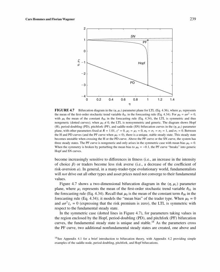
FIGURE 4.7 Bifurcation diagram in the (η,μ1) parameter plane for LTL (Eq. 4.36), where μ1 representsthe mean of the first-order stochastic trend variable ϑ01 in the forecasting rule (Eq. 4.34). For μ0 = aσ2 = 0,with μ0 the mean of the constant ϑ00 in the forecasting rule (Eq. 4.34), the LTL is symmetric and thusnongeneric (dotted curves); when μ0 = 0, the LTL is nonsymmetric and generic. The diagram shows Hopf(H), period-doubling (PD), pitchfork (PF), and saddle-node (SN) bifurcation curves in the (η,μ1) parameterplane, with other parameters fixed at R = 1.01, zs = 0, μ2 = μ3 = 0, σ0 = σ1 = σ2 = 1, and σ3 = 0. Betweenthe H and PD curves (and the PF curve when μ0 = 0), there is a unique, stable steady state. This steady statebecomes unstable when crossing the H or the PD curve. Above the PF curve or the SN curve, the system hasthree steady states. The PF curve is nongeneric and only arises in the symmetric case with mean bias μ0 = 0.When the symmetry is broken by perturbing the mean bias to μ0 = −0.1, the PF curve “breaks” into genericHopf and SN curves.

become increasingly sensitive to differences in fitness (i.e., an increase in the intensityof choice β) or traders become less risk averse (i.e., a decrease of the coefficient ofrisk-aversion a). In general, in a many-trader-type evolutionary world, fundamentalistswill not drive out all other types and asset prices need not converge to their fundamentalvalues.

Figure 4.7 shows a two-dimensional bifurcation diagram in the (η,μ1) parameterplane, where μ1 represents the mean of the first-order stochastic trend variable ϑ01 inthe forecasting rule (Eq. 4.34). Recall that μ0 is the mean of the constant term ϑ00 in theforecasting rule (Eq. 4.34); it models the “mean bias” of the trader type. When μ0 = 0and aσ2zs = 0 (expressing that the risk premium is zero), the LTL is symmetric withrespect to the fundamental steady state.

In the symmetric case (dotted lines in Figure 4.7), for parameters taking values inthe region enclosed by the Hopf, period-doubling (PD), and pitchfork (PF) bifurcationcurves, the fundamental steady state is unique and stable.18 As the parameters crossthe PF curve, two additional nonfundamental steady states are created, one above and

18See Appendix 4.1 for a brief introduction to bifurcation theory, with Appendix 4.2 providing simpleexamples of the saddle-node, period doubling, pitchfork, and Hopf bifurcations.


one below the fundamental. Another route to instability occurs when crossing the Hopfcurve, where the fundamental steady state becomes unstable and a (stable) invariantcircle with periodic or quasi-periodic dynamics is created. The pitchfork bifurcationcurve is nongeneric and occurs only in the symmetric case. When the symmetry isbroken by a nonzero mean bias μ0 = 0, as illustrated in Figure 4.7 (bold curves) for μ0 =−0.1, the PF curve disappears and “breaks” into two generic codimension bifurcationcurves: a Hopf and a saddle-node (SN) bifurcation curve. When crossing the SN curvefrom below, two additional steady states are created, one stable and one unstable. Noticethat, as illustrated in Figure 4.7, when the perturbation is small (in the figure, μ0 =−0.1), the SN and the Hopf curves are close to the PF and the Hopf curves (dotted lines)in the symmetric case. In this sense the bifurcation diagram depends continuously onthe parameters, and it is useful to consider the symmetric LTL as an “organizing” centerto study bifurcation phenomena in the generic, nonsymmetric LTL.

The most relevant case from an economic viewpoint arises when the mean μ1 of thefirst-order coefficient ϑ01 in the forecasting rule (Eq. 4.34) satisfies 0 ≤ μ1 ≤ 1. In thatcase, the (fundamental) steady state loses stability in a Hopf bifurcation as η increases.Figure 4.8 illustrates the dynamical behavior of the LTL as the parameter η further

(a) � 5 1.4 (b) � 5 1.51 (c) � 5 1.52

(d) � 5 1.57 (e) � 5 1.59 (f) � 5 1.6

FIGURE 4.8 Attractors in the phase space for the 5-D LTL with parameters R = 1.01, zs = 0, μ0 = 0,μ1 = 0, μ2 = μ3 = 0, and σ0 = σ1 = σ2 = σ3 = 1: (a) immediately after the Hopf bifurcation (quasi-)periodicdynamics on a stable invariant circle occurs; (b–c) after a Hopf bifurcation (quasi-)periodic dynamics on astable invariant torus occurs; and (d–f) breaking up of the invariant torus into a strange attractor.


increases. After the Hopf bifurcation periodic and quasi-periodic dynamics on a stableinvariant circle occur, and for increasing values of η, a bifurcation route to strange attrac-tors occurs. Figure 4.8 thus presents numerical evidence of the occurrence of a rationalroute to randomness, that is, a bifurcation route to strange attractors as the intensity ofchoice to switch forecasting strategies increases. If such rational routes to randomnessoccur for the LTL, the LTL convergence theorem implies that in evolutionary systemswith many trader types, rational routes to randomness occur with high probability.

Diks and van der Weide (2003, 2005) have generalized the notion of LTL andintroduced so-called continuous belief systems (CBS), where the beliefs of traders aredistributed according to a continuous density function. The beliefs distribution func-tion and the equilibrium prices coevolve over time. The LTL theory discussed here aswell as its extensions can be used to form a bridge between an analytical approach andthe literature on evolutionary artificial market simulation models reviewed in LeBaron(2000, 2006). See also Anufriev et al. (2008) for a recent application of a LTL in amacroeconomic model with heterogeneous expectations.

4.5. EMPIRICAL VALIDATION

In this section we discuss the empirical validity of the asset pricing model with het-erogeneous beliefs. There is already a large literature on heterogeneous agent modelsreplicating many of the important stylized facts of financial time series on short timescales (say, daily or higher frequency), such as fat tails and long memory in the returnsdistribution and clustered volatility. Examples of HAMs able to replicate stylized factsof financial markets include, for example, Brock and LeBaron (1996), Arthur et al.(1997), Brock and Hommes (1997b), Youssefmir and Huberman (1997), LeBaronet al. (1999), Lux and Marchesi (1999, 2000), Farmer and Joshi (2002), Kirmanand Teyssiere (2002), Hommes (2002), Iori (2002), Cont and Bouchaud (2000), andGaunersdorfer and Hommes (2007). The recent survey by Lux (2009) contains anextensive look at behavioral interacting agent models mimicking the stylized facts ofasset returns. We have already seen examples of simple heterogeneous agent mod-els mimicking temporary bubbles and crashes. In this section we discuss how thesequalitative features match observed bubbles and crashes in real markets.

Empirical validation and estimation of HAMs on economic or financial data arestill in their infancy. An early attempt has already been made by Shiller (1984) whopresented a HAM with smart money traders having rational expectations versus ordi-nary investors (whose behavior is in fact not modeled at all). Shiller estimated thefraction of smart money investors over the period 1900 to 1983 and found consider-able fluctuations of the fraction over a range between 0% and 50%. Baak (1999) andChavas (2000) estimated HAMs on hog and beef market data and found evidence forheterogeneity of expectations. Winker and Gilli (2001) and Gilli and Winker (2003)estimated the model of Kirman (1991, 1993) with fundamentalists and chartists, usingthe daily DM-US$ exchange rates from 1991 to 2000. Their estimated parameter val-ues correspond to a bimodal distribution of agents. Westerhoff and Reitz (2003) also


estimated an HAM with fundamentalists and chartists to exchange rates and found con-siderable fluctuations of the market impact of fundamentalists. Alfarno et al. (2005)estimated an agent-based herding model where agents switch between fundamentalistand chartist strategies. Branch (2004) estimated a model with heterogeneous beliefsand time-varying fractions, using survey data on inflation expectations. In this section,we discuss the estimation of a simple two-type asset-pricing model with heterogeneousbeliefs, as discussed in Section 4.2, on yearly S&P 500 data, 1871 to 2003, as done inBoswijk et al. (2007). As we will see, this simple two-type model can, for example,explain the dot-com bubble in the late 1990s and the subsequent crash starting at theend of 2000.19

4.5.1. The Model in Price-to-Cash Flows

In the previous sections, the dividend process of the risky asset has been assumed to bestationary. To estimate the model using yearly data of more than a century, the dividendprocess has to be taken growing over time and thus nonstationary. To estimate a simpletwo-type model, Boswijk et al. (2007) therefore reformulated the model in terms ofprice-to-cash flows. Recall from Eq. 4.5 that, under the assumption of zero net supplyof the risky asset, the equilibrium pricing equation is

pt =1

1 + r

H∑h=1

nh,tEh,t(pt+1 + yt+1) (4.38)

or equivalently

r =H∑h=1

nh,tEh,t[pt+1 + yt+1 − pt]

pt(4.39)

In equilibrium the average required rate of return for investors to hold the risky assetequals the discount rate r. In the estimation of the model, the discount rate r has been setequal to the sum of the (risk-free) interest rate and the required risk premium on stocks.A simple, nonstationary process that fits cash flow data (dividends or earnings) well isa stochastic process with a constant growth rate. More precisely, assume that log yt is aGaussian random walk with drift; that is,

log yt+1 = μ + log yt + υt+1 υt+1 ∼ i.i.d. N (0, σ2υ ) (4.40)

which impliesyt+1

yt= eμ+υt+1 = eμ+

12 σ

2υ eυt+1− 1

2 σ2υ = (1 + g)εt+1 (4.41)

19Van Norden and Schaller (1999) estimate a nonlinear time-series switching model with two regimes, anexplosive and a collapsing bubble regime, with the probability of being in the explosive regime dependingnegatively on the relative absolute deviation of the bubble from the fundamental. Brooks and Katsaris (2005)extend this model to three regimes, adding a third dormant bubble regime where the bubble grows at therequired rate of return without explosive expectations.


where g = eμ+12 σ

2υ − 1 and εt+1 = eυt+1+ 1

2 σ2υ , so that Et(εt+1) = 1. As before, we assume

that all types have correct beliefs on the cash flow; that is,

Eh,t[yt+1] = Et[yt+1] = (1 + g)ytEt[εt+1] = (1 + g)yt (4.42)

Since the cash flow is an exogenously given stochastic process, it seems natural toassume that agents have learned the correct beliefs on next period’s cash flow yt+1.In particular, boundedly rational agents can learn about the constant growth rate by, forexample, running a simple regression of log(yt/yt−1) on a constant.

In contrast, prices are determined endogenously and are affected by expectationsabout next period’s price. In a heterogeneous world, agreement about future pricestherefore seems more unlikely than agreement about future cash flows. Therefore weassume homogeneous beliefs about future cash flow but heterogeneous beliefs aboutfuture prices.20 The pricing Eq. 4.38 can be reformulated in terms of a price-to-cash-flow (P/Y) ratio, δt = pt/yt, as21

δt =1R∗

{1 +

H∑h=1

nh,tEh,t[δt+1]

}R∗ =

1 + r1 + g

(4.43)

In the special case, when all agents have rational expectations, the equilibrium pric-ing Eq. 4.38 simplifies to pt = (1/(1 + r))Et(pt+1 + yt+1). It is well known that, in thecase of a constant discount rate r and a constant growth rate g for dividends, according tothe static Gordon growth model (Gordon, 1962), the rational expectations fundamentalprice, p∗t , of the risky asset is given by

p∗t =1 + gr − g yt r > g (4.44)

Equivalently, in terms of price-to-cash-flow ratios, the fundamental is

δ∗t =p∗tyt

=1 + gr − g ≡ m (4.45)

We refer to p∗t as the fundamental price and to δ∗t as the fundamental P/Y ratio. Whenall agents are rational, the pricing Eq. 4.43 in terms of the P/Y ratio, δt = pt/yt, becomes

δt =1R∗

{1 + Et[δt+1]} (4.46)

20Barberis et al. (1998) consider a model in which agents are affected by psychological biases in formingexpectations about future cash flows. In particular, agents may overreact to good news about economic fun-damentals because they believe that cash flows have moved into another regime with higher growth. Theirmodel is able to explain continuation and reversal of stock returns.21In what follows we use either price-to-dividend (P/D) or price-to-earnings (P/E) ratios and use the generalnotation P/Y for price-to-cash flows.


In terms of the deviation from the fundamental ratio, xt = δt − δ∗t = δt − m, thissimplifies to

xt =1R∗Et[xt+1] (4.47)

Under heterogeneity in expectations, the pricing Eq. 4.43 is expressed in terms of xt as

xt =1R∗

H∑h=1

nh,tEh,t[xt+1] (4.48)

Heterogeneous Beliefs

The expectation of belief type h about next period P/Y ratio is expressed as

Eh,t[δt+1] = Et[δ∗t+1] + fh(xt−1, . . ., xt−L) = m + fh(xt−1, . . ., xt−L) (4.49)

where δ∗t represents the fundamental price-to-cash-flow ratio P/Y, Et(δ∗t+1) = m is therational expectation of the P/Y ratio available to all agents, xt is the deviation of theP/Y ratio from its fundamental value, and fh(·) represents the expected transitory devi-ation of the P/Y ratio from the fundamental value, depending on L past deviations. Theinformation available to investors at time t includes present and past cash flows and pastprices. In terms of deviations from the fundamental P/Y ratio, xt, we get

Eh,t[xt+1] = fh(xt−1, . . ., xt−L) (4.50)

Note again that the rational expectations fundamental benchmark is nested in theheterogeneous agent model as a special case when fh ≡ 0 for all types h. We can expressEq. 4.48 as

R∗xt =H∑h=1

nh,tfh(xt−1, . . ., xt−L) (4.51)

From this equilibrium equation it is clear that the adjustment toward the fundamentalP/Y ratio will be slow if a majority of investors has persistent beliefs about it.

Evolutionary Selection of Expectations

In addition to the empirical evidence of persistent deviations from fundamentals thereis also significant evidence of time variation in the sentiment of investors. This hasbeen documented, for example, by Shiller (1987, 2000) using survey data. In the modelconsidered here, agents are boundedly rational and switch between different forecastingstrategies according to recently realized profits. We denote by πh,t−1 the realized profits


of type h at the end of period t − 1, given by (see Eq. 4.14):

πh,t−1 = Rt−1zh,t−2 = Rt−1Eh,t−2[Rt−1]aVt−2[Rt−1]

(4.52)

where Rt−1 = pt−1 + yt−1 − (1 + r)pt−2 is the realized excess return at time t − 1 andzh,t−2 is the demand of the risky asset by belief type h, as given in Eq. 4.3, formed inperiod t − 2.

As before, we assume that the beliefs about the conditional variance of excessreturns are the same for all types and equal to fundamentalists beliefs about conditionalvariance, that is,

Vh,t−2[Rt−1] = Vt−2[P ∗t−1 + yt−1 − (1 + r)P ∗t−2] = y2t−2η

2 (4.53)

where η2 = (1 + m)2(1 + g)2Vt−2[εt−1], with εt IID noise driving the cash flow. Thefitness measure can be rewritten in terms of the deviation xt = δt − m of the P/Y ratiofrom its fundamental value, with m = (1 + g)/(r − g), as

πh,t−1 =(1 + g)2

aη2

(xt−1 − R∗xt−2

) (Eh,t−2[xt−1] −R∗xt−2

)(4.54)

This fitness measure has a simple, intuitive explanation in terms of forecasting per-formance for next period’s deviation from the fundamental. A positive demand zh,t−2

may be seen as a bet that xt−1 would go up more than what was expected on aver-age from R∗xt−2. (Note that R∗ is the growth rate of rational bubble solutions.) Therealized fitness πh,t−1 of strategy h is the realized profit from that bet and it will bepositive if both the realized deviation xt−1 > R

∗xt−2 and the forecast of the deviationEh,t−2[xt−1] > R∗xt−2. More generally, if both the realized absolute deviation |xt−1|and the absolute predicted deviation |Eh,t−2[xt−1]| to the fundamental value are largerthan R∗ times the absolute deviation |xt−2|, strategy h generates positive realized fit-ness. In contrast, a strategy that wrongly predicts whether the asset price mean revertsback toward the fundamental value or moves away from it generates a negative realizedfitness.

At the beginning of period t, investors compare the realized relative performances ofthe various strategies and withdraw capital from those that performed poorly and moveit to better strategies. The fractions nh,t evolve according to a discrete choice model withmultinomial logit probabilities, that is (see Eq. 4.13),

nh,t =exp[βπh,t−1]∑Hk=1 exp[βπk,t−1]

=1

1 +∑k =h exp[−βΔπh,k

t−1](4.55)

where β > 0 is the intensity of choice as before, and Δπh,kt−1 = πh,t−1 − πk,t−1 denotes the

difference in realized profits of belief type h compared to type k.


4.5.2. Estimation of a Simple Two-Type Example

Consider the case of two types, both predicting next period’s deviation by extrapolatingpast realizations in a linear fashion, that is,22

Eh,t[xt+1] = fh(xt−1) = ϕhxt−1 (4.56)

The dynamic asset-pricing model with two types can then be written as

R∗xt = ntϕ1xt−1 + (1 − nt)ϕ2xt−1 + εt (4.57)

where ϕ1 and ϕ2 denote the coefficients of the two belief types, nt represents the fractionof investors that belong to the first type of traders and εt represents a disturbance term.The value of the parameter ϕh can be interpreted as follows: If it is positive and smallerthan 1, investors expect the stock price to mean-revert toward the fundamental value.This type of agent represents fundamentalists because they expect the asset price tomove back toward its fundamental value in the long run. The closer ϕh is to 1, the morepersistent are the expected deviations. If the beliefs parameter ϕh is larger than 1, itimplies that investors believe the deviation of the stock prices will grow over time at aconstant speed. We will refer to this type of agent as a trend follower. Note in particularthat when one group of investors believes in a strong trend, that is, ϕh > R∗, this maycause asset prices to deviate further from their fundamental value. In the case with twotypes with linear beliefs (Eq. 4.56), the fraction of Type 1 investors is

nt =1

1 + exp{−β∗ [(ϕ1 − ϕ2)xt−3(xt−1 − R∗xt−2)]} (4.58)

where β∗ = β(1 + g)2/(aη2).The two-type model (Eqs. 4.57 and 4.58) has been estimated using an updated ver-

sion of the dataset described in Shiller (1989), consisting of annual observations of theS&P 500 index from 1871 to 2003. Here we present the estimation results with earn-ings as cash flows, but using dividends as cash flows gives similar results. The valuationratios are then the P/E ratios.23

Recall that according to the static Gordon growth model, the fundamental price isgiven by

p∗t = myt m =1 + gr − g (4.59)

The fundamental value of the asset is a multiple m of its cash flow, where m dependson the discount rate r and the cash-flow growth rate g. The multiple m can also be

22In the estimation of the model, higher-order lags turned out to be insignificant, so we focus on the simplestcase with only one lag in the function fh(·), with ϕh the parameter characterizing the strategy of type h.23Since earnings data are noisy, to determine the fundamental valuation we follow the practice of Campbelland Shiller (2005) to smooth earnings by a 10-year moving average.


interpreted as the P/D or the P/E ratios implied by the present value model. Figure 4.9shows the (log) of yearly S&P 500 data together with the fundamental benchmark aswell as their P/E ratios. The figure shows a clear long-term comovement of the stockprice and the fundamental value. However, the P/E ratio takes persistent swings awayfrom the constant value predicted by the present-value model. This suggests that thefundamental value does not account completely for the dynamics of stock prices, aswas suggested in the early debate on mean reversion by Summers (1986). A survey ofthe ongoing debate is given in Campbell and Shiller (2005). Here we use the simple

1880 1900 1920 1940

(a)

(b)

1960 1980 2000

4.0

4.5

5.0

5.5

6.0

6.5

7.0

7.5S&P 500Fund. value

PY ratioFund. ratio

1880 1900 1920 1940 1960 1980 2000

10

20

30

40

50

FIGURE 4.9 Yearly S&P 500, 1871–2003, and benchmark fundamental p∗t = myt, with m = (1 + g)/(1 + r). (a) shows logs of S&P 500 and the log of the fundamental p∗t ; (b) shows the P/E-ratio of the S&P500 around the constant fundamental benchmark p∗t /yt = m.


constant-growth Gordon model for the fundamental price and estimate the two-typemodel on deviations from this benchmark.24

Recall that R∗ = (1 + r)/(1 + g), where g is the constant growth rate of the cashflow and r is the discount rate equal to the risk-free interest rate plus a risk premium.We use an estimate of the risk premium—the difference between the expected return onthe market portfolio of common stocks and the risk-free interest rate—to obtain R∗, asin Fama and French (2002). The risk premium safisfies

RP = g + y/p − i (4.60)

where g is the growth rate of dividends, y/p denotes the average dividend yield yt/pt−1

and i is the risk-free interest rate. For annual data from 1871 to 2003 of the S&P 500,the estimates are i = 2.57% andRP = 6.56% so that r = 9.13% andR∗ = 1.074.25 Thecorresponding average P/E ratio is 13.4, as illustrated in Figure 4.9.

Using yearly data of the S&P 500 index from 1871 to 2003, the parameters(ϕ′1,ϕ′2, β∗) in the two-type model (Eqs. 4.57 and 4.58) can be estimated by nonlinearleast squares. The estimation results are as follows:

R∗xt = nt{0.80 xt−1}(0.074)

+ (1 − nt){1.097 xt−1} + εt(0.052)

(4.61)

nt = {1 + exp[−7.54(−0.29xt−3 )(4.93)

(xt−1 − R∗xt−2)]}−1

R2 = 0.77, AIC = 2.23, AICAR(1) = 2.29, ϕAR(1) = 0.983,

QLB (4) = 0.94, F boot(p-value) = 10.15 (0.011)

The belief coefficients are highly significant and different from each other. On theother hand, the intensity of choice β∗ is not significantly different from zero. Thisis a common result in nonlinear switching-type regression models, where the param-eter β∗ in the transition function is difficult to estimate and has a large standarddeviation because relatively large changes in β∗ cause only a small variation of thefraction nt.

Terasvirta (1994) argues that this should not be worrying as long as there is signifi-cant heterogeneity in the estimated regimes. The nonlinear switching model achievesa lower value for the AIC selection criterion compared to a linear AR(1) model. Thissuggests that the model is capturing nonlinearity in the data. This is also confirmed bythe bootstrap F-test for linearity, which strongly rejects the null hypothesis of linearity

24The same approach can be used for more general, time-varying fundamental processes. Manzan (2003)shows that a dynamic Gordon model for the fundamental price, where the discount rate r and/or the growthrate g are time varying, does not explain the large fluctuations in price-to-cash-flow ratios and in fact yieldsa fundamental price pattern close to that for the static Gordon model. Boswijk et al. (2007) also estimate aversion of the model allowing for time variation in the growth rate of the cash flow and obtain similar results.25These estimates are slightly different from Fama and French (2002) because, as in Shiller (1989), we usethe CPI index to deflate nominal values.


in favor of the heterogeneous agent model. The residuals of the regression do not showsignificant evidence of autocorrelation at the 5% significance level.

The estimated coefficient of the first regime is 0.80, corresponding to a half-lifeof about three years. The first regime can be characterized as fundamentalist beliefs,expecting the asset price to move back toward its fundamental value. In contrast, thesecond regime has an estimated coefficient close to 1.1, implying that in this regimeagents are trend followers, believing the deviation of the stock price to grow over timeat a constant speed larger than R∗ ≈ 1.074. At times when the fraction of investorsusing this belief is equal or close to 1, we have explosive behavior in the P/E ratio.The sentiment of investors switches between a stable fundamentalists regime and atrend-following regime. In normal periods agents consider the deviation a temporaryphenomenon and expect it to quickly revert to fundamentals. In other periods, a rapidincrease in stock prices not paralleled by improvements in the fundamentals causeslosses for fundamentalists and profits for trend followers. Evolutionary pressure willthen cause more fundamentalists to become trend followers, thus reinforcing the trendin prices.

Figure 4.10 shows the time series of the fraction of fundamentalists and the averagemarket sentiment, defined as

ϕt =ntϕ1 + (1 − nt)ϕ2

R∗(4.62)

It is clear that the fraction of fundamentalists varies considerably over time, with peri-ods in which it is close to 0.5 and other periods in which it is close to either of theextremes 0 or 1. The series of the average market sentiment shows that there is sig-nificant time variation between periods of strong mean reversion when the market isdominated by fundamentalist and other periods in which ϕt is close to or exceeds 1and the market is dominated by trend followers. These plots also offer an explanationof the events of the late 1990s: For six consecutive years the trend-following strategyoutperformed the fundamentalist strategy and a majority of agents switched to the trend-following strategy, driving the average market sentiment beyond 1 and thus reinforcingthe strong price trend. However, at the turn of the market in 2000, the fraction of funda-mentalists increased again, approaching 1 and thus contributing to the reversal towardthe fundamental value in subsequent years.

The estimation results show that there are two different belief strategies: one inwhich agents expect continuation of returns and the other in which they expect reversal.We also find that there are some years in which one type of expectation dominatesthe market. It is clear that the expectation of continuation of positive returns domi-nated the market in the late 1990s, with the average market sentiment coefficient ϕt inEq. 4.62 larger than 1 in the late 1990s. Despite the awareness of the mispricing, in thisperiod investors were aggressively extrapolating the continuation of the extraordinaryperformances realized in the previous years. Our approach endogenizes the switchingof agents among beliefs. The evolutionary mechanism that relates predictor choice totheir past performance is supported by the data. It also confirms previous evidence thatpointed in this direction.


1880 1900 1920 1940

(a)

(b)

1960 1980 2000

0.0

0.2

0.4

0.6

0.8

1.0

n t

1880 1900 1920 1940 1960 1980 2000

0.7

0.8

0.9

1.0

1.1

�t

FIGURE 4.10 Estimated fraction nt of fundamentalists (a) and market sentiment factor ϕt (b) in(Eq. 4.62) in two-type model.

Based on answers to a survey, Shiller (2000) constructed indices of “bubble expec-tations” and “investor confidence.” In both cases, he found that the time variation inthe indices is well explained by the lagged change in stock prices. Based on a differ-ent survey, Fisher and Statman (2002) found that in the late 1990s individual investorshad expectations of continuation of recent stock returns while institutional investorswere expecting reversals. This is an interesting approach to identifying heterogeneity ofbeliefs based on the type of investors rather than the type of beliefs. In the view of ourmodel, the bubble in the 1990s was triggered by good news about economic fundamen-tals (a new Internet technology) and strongly reinforced by trend extrapolating behavior.The bubble was reversed by bad news about economic fundamentals (excessive growthcannot last forever and is not supported by earnings), and the crash was accelerated byswitching of beliefs back to fundamentals.


4.5.3. Empirical Implications

In this subsection we discuss some empirical implications of the estimation of ournonlinear evolutionary switching model with heterogeneous beliefs. First, we investi-gate the response to a positive shock to fundamentals when the asset is overvalued.Second, we address the question concerning the probability that a bubble may resumeby considering the evolution of the valuation ratios conditional on data until the end of2003. These simulation experiments both show the importance of considering nonlineareffects in the dynamics of stock prices.

Response to a Fundamental Shock

We use the estimated parameters to investigate the response of the market valuation togood news. Assume that at the beginning of period t the cash flow increases due toa permanent increase in its growth rate. This implies that the asset has a higher fun-damental valuation ratio, but what is the effect on the market valuation? We addressthis question both for the nonlinear switching model and a linear benchmark. The lin-ear model may be interpreted as a model with a representative agent believing in anaverage mean reversion toward the fundamental.26 Assume that at t − 1 the funda-mental valuation ratio was 15 and the good news at time t drives it to 17. Assumealso that the equilibrium price at t − 1 was 16. Figure 4.11 shows the valuation ratiodynamics in response to the good news for both the linear and the nonlinear switchingmodels.

The figure shows the average price path over 2000 simulations of the estimatedmodels. There is a clear difference between the linear and the nonlinear models. In thelinear case, the positive shock to the fundamental value leads to an immediate increaseof the price followed by mean-reversion thereafter. In contrast, for the nonlinear het-erogeneous agent model, the pattern that emerges is consistent with the evidence ofshort-run continuation of positive returns and long-term reversal. After good news, theagents incorporate the news into their expectations and they expect that part of the previ-ous period overvaluation will persist. One group—the trend followers—overreacts andexpects a further increase of the price, while the other group—the fundamentalists—expects the price to diminish over time. The equilibrium price at time t overshoots andalmost reaches 18. In the following two periods trend followers continue to buy thestock and drive its price and its valuation ratio even higher. Finally, the reversal startsand drives the ratio back to its long-run fundamental value. Initially, the aggressiveinvestors interpret the positive news as a confirmation that the stock overvaluation wasjustified by forthcoming news. However, the lack of further good news convinces mostinvestors to switch back to the mean-reverting expectations and the stock price is drivenback toward its fundamental value.

26The linear benchmark is, for example, obtained for β = 0 or equivalently when both fractions nt = 1 − nt =0.5 in Eq. 4.57. Hence, in the linear model there is no strategy switching between different types but rather arepresentative agent with a linear forecasting rule.


0 5 10 15 20 25 30

15

16

17

18

19

20

FIGURE 4.11 Average response (over 2000 simulations) to a shock to the fundamental for the linear rep-resentative agent model (dashed line) and the nonlinear two-type switching model (dotted line with circles).At period 0 there is a permanent shock to the fundamental price from 15 to 17. The simulation uses the esti-mated parameter values for the P/D ratio, with a representative agent average belief parameter ϕ = 0.968 andheterogeneous agent parameters ϕ1 = 0.762 and ϕ2 = 1.135 for the two types. The nonlinear heterogeneousagent model exhibits short-run continuation of positive returns and long-term reversal.

Will the Bubble Resume?

As a model forecasting exercise, we simulate the evolution of the valuation ratios usingthe estimated heterogeneous agent model. We then obtain the predicted evolution ofthe valuation ratio conditional on the value realized at the end of 2003. Innovations areobtained by reshuffling the estimated residuals. Instead of focusing our attention onlyon the mean or the median of the distribution, we consider the quantiles correspondingto 10%, 30%, 50%, 70%, and 90% probability over 2000 replications of the estimatedmodel in Eq. 4.61 for the P/E ratio. In addition to the quantiles predicted by our non-linear model, we also plot those predicted by the linear representative agent model.Figure 4.12 shows the 1- to 5-year periods ahead quantiles of the estimated model’spredictive distribution.

The linear model—Figure 4.12(a)—predicts that the valuation ratio reverts towardthe mean at all quantiles considered. In contrast, the nonlinear switching model predictsthat there is a significant probability that the ratio may increase again as a result of theactivation of the trend-following regime. The 70% and 90% quantiles clearly show thatthe PD ratio may increase again to levels close to 35. Stated differently, our heteroge-neous agent model predicts that with probability over 30% the PD ratio may increase tomore than 30. Note, however, that the median predicts that the ratio should decrease asimplied by the linear mean-reverting model.

Another implication of our model is that if the first (mean-reverting) regime domi-nates the beliefs of investors, it will enforce a much faster adjustment than predictedby the linear model. This is clear from the bottom quantiles of the distributions. These


(b)1985 1987 1989 1991 1993 1995 1997 1999 2001 2003 2005 2007

10

15

20

25

30

35

40

45

50

90% 70% Median

(a)

1985 1987 1989 1991 1993 1995 1997 1999 2001 2003 2005 2007

10

15

20

25

30

35

40

45

50

90% 70% Median

FIGURE 4.12 Prediction of P/E ratios five years ahead, based on linear representative agent model (a) and nonlinear two-typeswitching model (b). The estimated belief parameters are ϕ = 0.983 for the representative agent and ϕ1 = 0.80 and ϕ2 = 1.097 forthe two-type switching model. The quantiles corresponding to 10, 30, 50, 70, and 90% probability over 2000 replications are shown.The realized P/E ratios, 2004–2006, are also indicated and show that the realized P/E ratio for 2006 falls outside the 10% quantileof the linear model.

simulations show that predictions from a linear, representative agent model versus anonlinear, heterogeneous agent model are quite different. In particular, extreme eventswith large deviations from the benchmark fundamental valuation are much more likelyin a nonlinear world.

4.6. LABORATORY EXPERIMENTS

Asset-pricing models with heterogeneous beliefs exhibit interesting dynamics char-acterized by temporary bubbles and crashes, triggered by news about fundamentalsand reinforced by self-fulfilling expectations and trend-following investment strategies.The previous section focused on the empirical relevance of such models; this sec-tion confronts the model with data from laboratory experiments with human subjects.Laboratory experiments are well suited to discipline the class of behavioral modes


(or heuristics) boundedly rational subjects may use in economic decision making. Here,we discuss a number of “learning to forecast experiments” in which subjects mustforecast the price of an asset for which the realized market price is an aggregation ofindividual expectations.

In real markets, it is hard to obtain detailed information about investors’ individualexpectations. One approach is to collect survey data on individual expectations, as donefor example by Turnovsky (1970) on expectations about the Consumer Price Index andthe unemployment rate during the post-Korean War period. Frankel and Froot (1987a,b,1990a,b), Allen and Taylor (1990), Ito (1990), and Taylor and Allen (1992) use a surveyon exchange rate expectations and conclude that financial practitioners use differentforecasting and trading strategies. A consistent finding from survey data is that at shorthorizons, investors tend to use extrapolative chartists’ trading rules, whereas at longerhorizons investors tend to use mean-reverting fundamentalists’ trading rules. Shiller(1987, 1990, 2000) analyzes surveys on expectations about stock market prices andreal estate prices and finds evidence for time variation in investors’ sentiment; see alsoVissing-Jorgensen (2003).

Laboratory experiments with human subjects provide an alternative, complementaryapproach to study the interaction of individual expectations and the resulting aggregateoutcomes. An important advantage of the experimental approach is that the experi-menter has full control over the underlying economic fundamentals. Surprisingly littleexperimental work has focused on expectation formation in markets. Williams (1987)considers expectation formation in an experimental double auction market that variesfrom period to period by small shifts in the market-clearing price. Participants predictthe mean contract price for four or five consecutive periods. The participant with thelowest forecast error earns $1.00.

In Smith, Suchanek, and Williams (1998), expectations and the occurrence of spec-ulative bubbles are studied in an experimental asset market. In a series of papers,Marimon, Spear, and Sunder (1993) and Marimon and Sunder (1993, 1994, 1995)studied expectation formation in inflationary overlapping generations’ economies.Marimon, Spear, and Sunder (1993) find experimental evidence for expectationallydriven cycles and coordination of beliefs on a sunspot two-cycle equilibrium but onlyafter agents have been exposed to exogenous shocks of a similar kind. Marimon andSunder (1995) present experimental evidence that a “simple” rule, such as a constantgrowth of the money supply, can help coordinate agents’ beliefs and help stabilize theeconomy. Duffy (2006, 2008) gives stimulating surveys of laboratory experiments invarious macro settings and how individual and aggregate behavior could be explainedby agent-based models.

However, most of these papers cannot be viewed as pure experimental testing ofthe expectations hypothesis, everything else being constant, because in the experimentsdynamic market equilibrium is affected not only by expectations feedback but alsoby other types of human decisions, such as trading behavior. A number of laboratoryexperiments have focused on expectation formation exclusively. Schmalensee (1976)presented subjects with historical data on wheat prices and asked them to predict the


mean wheat price for the next five periods. In Dwyer et al. (1993) and Hey (1994),subjects had to predict a time series generated by a stochastic process such as a randomwalk or a simple linear first-order autoregressive process; in the last two papers noeconomic context was given. Kelley and Friedman (2002) considered learning in anorange juice futures price-forecasting experiment, where prices were driven by a lin-ear stochastic process with two exogenous variables (weather and competing supply).A drawback common to these papers is that the historical or stochastic price series areexogenous and there is no feedback from subjects’ forecasting behavior.

4.6.1. Learning to Forecast Experiments

In the remaining part of this section we mainly focus on the learning-to-forecast exper-iments in Hommes et al. (2005). In these experiments, subjects forecast the price ofa risky asset, which is determined by market clearing with feedback from individ-ual expectations. Similar experiments have been performed by van de Velden (2001),Gerber et al. (2002), Sutan and Willinger (2005), Adam (2007), Hommes et al. (2007),and Heemeijer (2007); see also the recent survey in Duffy (2008). We are particularlyinterested in the following questions:

• How do boundedly rational agents form individual expectations, and how do theylearn in a heterogeneous world?

• How do individual forecasting rules interact, and what is the aggregate outcome ofthese interactions?

• Will coordination occur, even when there is limited market information?• Does learning enforce convergence to rational expectations equilibrium?

In real financial markets, traders are involved in two related activities: prediction andtrade. Traders make a prediction concerning the future price of an asset, and given thisprediction, they make a trading decision. In the experiments discussed here, the onlytask of the subjects is to forecast prices; asset trading is computerized and derived fromoptimal demand (from mean-variance maximization), given the individual forecast. Theexperiments can therefore be seen as learning to forecast experiments (Marimon andSunder 1994, p. 134), in contrast to learning to solve intertemporal optimization prob-lems or, more concisely, learning to optimize experiments (Duffy 2006, p. 4), whereparticipants are asked to submit their decisions (e.g., trading or consumption quantities)while their private beliefs about future developments remain implicit. Learning to fore-cast experiments provide us with “clean” data on expectations, which can be used totest various expectations hypotheses.

In the experiments, each participant is told that he or she is an advisor to a pensionfund, with the only task to predict next period’s price of a risky asset. Earnings are givenby a (truncated) quadratic scoring rule:

eht = max{

1300 − 130049

(pt − peht

)2, 0}

(4.63)


where 1300 points is equivalent to 0.5 euros, and earnings are 0 in period t when∣∣pt − peht∣∣ ≥ 7. Subjects are informed that their pension fund needs to decide how muchto invest in a risk-free asset paying a risk-free gross rate of return R = 1 + r, where r isthe real interest rate, and how much to invest in shares of an infinitely lived risky asset.The risky asset pays uncertain IID dividends yt with mean y. The mean dividend y andthe interest rate r are common knowledge, so that the subjects could compute the (con-stant) fundamental p∗ = y/r = 3/0.05 = 60. Subjects know that the price of the asset isdetermined by market clearing. Although they do not know the exact underlying market-clearing equation, they have qualitative information about the market and are informedthat the higher their forecast, the larger will be the fraction of money of their pensionfund invested in the risky asset and the larger will be the demand for stocks. They do notknow the exact investment strategy of their pension fund and the investment strategiesof the other pension funds. They also do not know the number of pension funds (whichis six) or the identity of the other members of the group.

The experiment lasts for 51 periods. In every period t the participants have to predictthe price pt+1 of the risky asset in period t + 1, given the available information consist-ing of past prices pt−1, pt−2, . . ., p1 and the participants’ own past individual predictionspeht, p

eh,t−1, . . ., peh1. Notice that the participants have to make a two-period-ahead forecast

for pt+1, since pt−1 is the latest available price observation. Subjects are told that theirprice forecast has to be between 0 and 100 for every period. In periods 1 and 2, noinformation about past prices is available. At the end of period t, when all predictionsfor period t + 1 have been submitted, the participants are informed about the price inperiod t and earnings for that period are revealed. On their computer screens, the sub-jects are informed about their earnings in the previous period, total earnings, a table ofthe last 20 prices, and their corresponding predictions and time series of the prices andtheir predictions. Subjects have no information about earnings and predictions of others.

4.6.2. The Price-Generating Mechanism

The asset market is populated by six pension funds and a small fraction of fundamen-talist robot traders. Each pension fund h is matched with a participant and makes aninvestment decision at time t based on this participant’s prediction peh,t+1 of the assetprice. The fundamentalist trader always predicts the fundamental price pf and tradesbased on this prediction.

The realized asset price in the experiment is determined by market clearing, withthe pension fund’s asset demand derived from mean-variance maximization, given theiradvisor’s forecast, as in the standard asset-pricing model with heterogeneous beliefs(e.g., Campbell, Lo, and MacKinlay, 1997; Brock and Hommes, 1998; see Section 4.2).The market-clearing price is given by Eq. 4.5:

pt =1

1 + r[(1 − nt) pt] (4.64)

where pet+1 = 16

∑6h=1 p

eh,t+1 is the average forecast for period t + 1 of the six partici-

pants, nt is the time-varying weight of the fundamentalist traders, and εt is a noise term,


representing (small) stochastic demand and supply shocks. Note that the realized assetprice pt at time t is determined by the individual price predictions ph,t+1 for time t + 1.Therefore, when traders have to make a prediction for the price in period t + 1, they donot know the price in period t yet, and they can only use information on prices up totime t − 1.

The weight nt of the fundamental traders in the market is endogenous and dependspositively on the absolute distance between the asset price and the fundamental valueaccording to:

nt = 1 − exp(− 1

200

∣∣pt−1 − pf∣∣) (4.65)

The greater this distance, the more the fundamentalist trader will buy or short the asset.The fundamentalist trader therefore acts as a “stabilizing force” pushing prices in thedirection of the fundamental price. Their presence excludes the possibility of everlastingspeculative bubbles in asset prices.27 Also note that nt = 0, if pt−1 = pf.

An important feature of the asset-pricing model is its self-confirming nature or posi-tive feedback: If all traders make a high (low) prediction, the realized price will also behigh (low). This feature is characteristic for speculative asset markets: If traders expecta high price, the demand for the risky asset will be high, and as a consequence therealized market price will be high, assuming that the supply is fixed.

4.6.3. Benchmark Expectations Rules

Figure 4.13 shows the price dynamics under three benchmark expectation rules: rationalexpectations, naıve expectations, and a trend extrapolation rule. In the rational expec-tations’ benchmarks, all agents forecast the price to be equal to its fundamental valuepf = 60.28 Realized prices are then given by

pt = pf +1

1 + rεt (4.66)

Therefore, under rational expectations, prices exhibit small random fluctuations aroundthe fundamental price pf = 60. This outcome of the experiment should probably notbe expected right from the start, but perhaps subjects can learn to coordinate on therational, fundamental forecast.

27DeGrauwe et al. (1993) discuss a similar stabilizing force in an exchange rate model with fundamental-ists and chartists. In the same spirit, Kyle and Xiong (2001) introduce a long-term investor who holds arisky asset in an amount proportional to the spread between the asset price and its fundamental value. Sincein the experiments the fundamental value is pf = 60, the weight of the fundamentalist traders is boundedabove by n = 1 − exp

(− 310

) ≈ 0.26. The weight of the other traders is the same for each trader and equal to(1 − nt) /6 ≤ 0.17.28Recall that participants know the values of y and r and therefore have enough information to compute thefundamental value and predict it for any period.


(b) (c)

0 25Time Time

Pric

e

Pric

e

5145

50

55

60

65

70NaÏve expectations

0 25 5145

50

55

60

65

70AR-2 expectations

40

45

50

55

60

65

70

0 10 20 30 40 50

Pric

e

Time

(a)

Fundamental pricePrice under rational expectations

FIGURE 4.13 Realized prices under some benchmark expectation rules. (a) Under rational expecta-tions, prices remain very close to the fundamental price 60; (b) under naıve expectations, prices convergemonotonically, but slowly, toward the fundamental price; (c) under a simple linear AR-2 rule, pet+1 =(pt−1 + 60)/2 + (pt−1 − pt−2), which may be interpreted as an anchor and adjustment rule, prices exhibitpersistent oscillations.

Under naıve expectations all participants use the last observed price as their forecast,that is, peh,t+1 = pt−1. The asset price then converges (almost) monotonically toward thefundamental price, as illustrated in Figure 4.13. Finally, the figure also illustrates whathappens when all subjects use the simple trend extrapolation rule:

peh,t+1 =(60 + pt−1)

2+ pt−1 − pt−2 (4.67)

If all subjects use the forecasting rule (Eq. 4.67), realized market prices will fluctuatefor 50 periods. This simple rule may be viewed as an anchor and adjustment heuristic,following the terminology of Tversky and Kahneman (1974), since it uses an anchor(the average of the fundamental price and the last observed price) and extrapolates thelast price change from there. One may wonder how subjects would arrive at this anchor


if they do not know the fundamental, but quite surprisingly a number of subjects used arule very similar to Eq. 4.67.

4.6.4. Aggregate Behavior

Figure 4.14 shows time series of the realized asset prices and individual predictionsin the experiments for five different groups. The first three groups illustrate the threetypical qualitatively different outcomes in the treatment with robot traders:

• Monotonic convergence. The price converges (atmost) monotonically to the funda-mental price from below.

• Persistent oscillations. The price oscillates with more or less constant amplitude;there is no convergence of the price to its fundamental value.

• Dampened oscillations. The price oscillates around the fundamental price withlarge amplitude initially, but the amplitude decreases over time, indicating (slow)convergence to the fundamental price.

The last two groups in Figure 4.14 illustrate what happens in a different treatmentof the experiments without fundamental robot traders. When there are no fundamentalrobot traders present in the market, persistent price oscillations with large amplitudetypically occur. The difference between these last two groups lies in the upper boundfor price predictions, set to 100 (as in the case with robot traders) and 1000, respectively.Hommes et al. (2008) ran experiments without robot traders and a high upper bound of1000 (maintaining the same fundamental price pf = 60) and in six out of their sevenmarkets long-lasting price bubbles (almost) reaching the upper bound were observed,with price levels up to 15 times the fundamental value.

Comparing the experimental results in Figure 4.14 with the simulated benchmarks inFigure 4.13 one observes that realized prices under naıve expectations resemble real-ized prices in the case with monotonic convergence remarkably well. On the otherhand, the case of persistent oscillatory behavior in the experiment is qualitatively simi-lar to the asset price behavior when participants use a simple AR (2) prediction strategy.Clearly, naıve and AR (2) prediction strategies give a qualitatively much better descrip-tion of aggregate asset price fluctuations in the experiment than does the benchmarkcase of rational expectations. Recall from Subsection 4.6.3 that an AR (2) rule has asimple behavioral interpretation as an anchor and adjustment trend-following forecast-ing strategy.

4.6.5. Individual Prediction Strategies

In this subsection we discuss some characteristics and estimation of individualprediction strategies. Some participants try to extrapolate observed trends and by doingso overreact and predict too high or too low. Other participants are more cautiouswhen submitting predictions and use adaptive expectations, that is, an average of theirlast forecast and the last observed price. An individual degree of overreaction can be


40

45

50

55

60

65

70

40

45

50

55

60

65

70P

rice

Group 2

Fundamental price Experimental price

Pre

dict

ion

Group 2

Fundamental price Experimental price

40

45

50

55

60

65

70

40

45

50

55

60

65

70

Pric

e

Pre

dict

ion

Group 1 Group 1

Fundamental price Experimental price908070605040302010 0

20

40

60

80

100

Pric

e

Pre

dict

ion

0 10 20 30 40 50

Group 4

0 10 20 30 40 50

Group 4

Pric

e

Pre

dict

ion

0

20

40

60

80

100

2 4 6 8 10 12 14 16 18 20 22 24 26 28 30 32 34 36 38 40 42 44 46 48 50

Group 11, no robot

0

20

40

60

80

100

2 4 6 8 10 12 14 16 18 20 22 24 26 28 30 32 34 36 38 40 42 44 46 48 50

Group 11, no robot

Pric

e

Pre

dict

ion

0

200

400

600

800

1000

2 4 6 8 10 12 14 16 18 20 22 24 26 28 30 32 34 36 38 40 42 44 46 48 500

200

400

600

800

1000

2 4 6 8 10 12 14 16 18 20 22 24 26 28 30 32 34 36 38 40 42 44 46 48 50

Group 4, no robot, upper bound 1000 Group 4, no robot, upper bound 1000

FIGURE 4.14 Realized prices (a) and individual predictions (b) in five typical asset-pricing experiments. The fundamentalprice pf = 60 is indicated by a horizontal line. The first three examples show three different outcomes in the experiments withrobot traders: monotonic convergence, persistent oscillations, and dampened oscillations. The last two examples show experimentswithout robot traders for upper bounds of 100 and 1000, respectively. The right panels show a striking coordination of individualforecasts.

quantified as the average absolute (one-period) change in predictions of participant h:

eh =

141

51∑t=11

∣∣peht − peh,t−1

∣∣ (4.68)

The average absolute change in the price is given by = 141

∑51t=11 |pt − pt−1|. We

will say that individual h overreacts if eh > and we will say that individual h is


0

2

4

6

8

10

12

14

16

18

1 2 3 4 5 6 7 8 9 10

FIGURE 4.15 Individual degrees of overreactions for 10 different groups, all with a robot trader: the firstseven with a fundamental pf = 60 and the last three with a fundamental pf = 40. The line segments representthe average absolute price change; the dots represent the average absolute changes in individual forecasts.Dots above the line segments correspond to individual overreaction.

cautious if eh ≤ . Figure 4.15 illustrates the individual degree of overreaction for the

different groups. In the case of monotonic convergence (groups 2 and 5), there is nooverreaction; in the case of permanent oscillations (groups 1, 6, 8, and 9) a majorityof subjects shows some overreaction, but it is relatively small. In the case of dampenedoscillations (groups 4, 7, and 10), with large temporary bubbles in the initial phases ofthe experiment, a majority of participants strongly overreacts. Oscillatory behavior andtemporary bubbles are thus caused by overreaction of a majority of agents.

Individual prediction strategies have been estimated using a simple linear model:

peh,t+1 = αh +4∑i=1

βhipt−i +3∑j=0

γhjpeht−j + νt (4.69)

where νt is an IID noise term. This general setup includes several important specialcases: (1) naıve expectations (βh1 = 1, all other coefficients equal to 0); (2) adap-tive expectations (βh1 + γh0 = 1, all other coefficients equal to 0), and (3) AR (L)processes (all coefficients equal to 0, except αh, βh1, . . ., βhL). The estimation resultsfor 60 participants (using observations t = 11 to t = 51) can be summarized as follows:

• For more than 90% of the individuals, the simple linear rule (Eq. 4.69) describesforecasting behavior well.

• In the monotonically converging markets, a majority of subjects uses a naıve, anadaptive, or an AR(1) forecasting rule.

• In the dampened and persistently oscillating markets, a majority of subjects usessimple AR(2) or AR(3) forecasting rules; in particular, a number of subjects use asimple trend-following rule of the form:

peh,t+1 = pt−1 + δh (pt−1 − pt−2) δh > 0 (4.70)

This forecasting rule corresponds to positive feedback of momentum traders.


Within each group, participants learn to coordinate on a simple forecasting rule,which becomes self-fulfilling. If participants coordinate on an adaptive or AR(1) fore-casting rule, the asset price monotonically converges to the fundamental price. Incontrast, if the participants coordinate on a trend-following rule, transitory or evenpermanent price oscillations may arise, with persistent deviations from fundamentalprice. Anufriev and Hommes (2008) extended the adaptive belief systems in Section 4.2and developed an evolutionary heuristics-switching model, matching all three differentobserved patterns in the learning to forecasting experiments remarkably well.

4.6.6. Profitability

In the learning-to-forecast experiments, subjects have been rewarded by their forecast-ing performance. As discussed in Hommes (2001), the fitness measure of (minus)squared forecasting errors is equivalent to risk-adjusted profits, and therefore it maybe a relevant measure in real markets (see Footnote 6). But it is interesting to inves-tigate the corresponding realized profits of the pension funds. In this section thereforewe briefly discuss the profitability, that is, the (nonrisk-adjusted) realized profits, of theinvestment strategies. Realized profits of a mean-variance investment strategy based ona price forecast peh,t+1 are given by:

πht = (pt+1 + yt+1 − Rpt)(peh,t+1 + y −Rpt) (4.71)

As a typical example, Figure 4.16 shows the realized profits and the realized accu-mulated profits in group 4, that is, a group with a robot trader and upperbound 100exhibiting dampened price oscillations (the third panel in Figure 4.14). Figure 4.16shows the realized profits corresponding to the six individual forecasts, the realizedprofits of the fundamental robot trader, and the realized profits of a hypotheticalswitching strategy, together with the realized price series (scaled by a factor of 3).

Clearly there are large fluctuations in the realized profits and all strategies occasion-ally suffer from large losses. The fundamental strategy starts with positive profits inperiods 1 to 6 as the asset price rises from below the fundamental. When the asset pricerises above its fundamental value and the bubble starts, the fundamental strategy makeslarge losses in periods 7 to 13. At the peak of the first bubble, at period 13, the fun-damental strategy has performed second to last on average, with the second to lowestaccumulated realized profits. During the crash, however, the fundamentalists make hugeprofits because they have built a large short position in the risky asset. At the same time,most other (trend-following) strategies suffer large losses because they hold long posi-tions. As the crash continues and the asset price falls below its fundamental value, thefundamental strategy starts making losses again. At the bottom of the market in period19, fundamentalists make a large loss. Over the full sample of 50 periods, however, onaverage the fundamental strategy performs very well and accumulates more profits thanthe other six forecasting strategies. Figure 4.16 also shows that the fundamental strategyis beaten by a switching strategy, always selecting the best (according to last period’s


2400

0

400

800

5 10 15 20 25 30 35 40 45 50

PROFROBOT

PROFPREDMAX

PROF1

PROF2

PROF3

PROF4

PROF5

PROF6

PRICE3TIMES

ACPROFROBOT

ACPROFPREDMAX

ACPROF1

ACPROF2

ACPROF3

ACPROF4

ACPROF5

ACPROF6

2400

2200

0

200

400

600

800

2 4 6 8 10 12 14 16 18 20 22 24

24000

22000

0

2000

4000

6000

5 10 15 20 25

(a) (b)

30 35 40 45 5022000

21000

0

1000

2000

3000

2 4 6 8 10 12 14 16 18 20 22 24

FIGURE 4.16 Realized (nonrisk adjusted) profits (top panel) and accumulated profits (bottom panel) for group 4 (see Figure4.14) with a robot trader and price upper bound 100. The graphs in (a) show periods 1–50; (b) graphs zoom in to periods 1–25;the realized price series (scaled by a factor of 3) is also shown. The top graphs show the realized profits corresponding to the sixindividual forecasting strategies, the fundamental robot trader, and a hypothetical switching strategy using the best (according tolast period’s realized profits) of the other seven strategies. The bottom graphs show the accumulated profits of these eight strategies.Realized profits exhibit large fluctuations over time, and all strategies at times suffer from large losses. On average and in terms ofaccumulated profits, the fundamental strategy performs very well but is beaten by the switching strategy.

realized profit) out of the seven other strategies. Stated differently, the switching strat-egy always uses the forecast of the advisor whose pension fund generated the highestrealized profit in the previous period. Such a switching strategy beats the fundamentalrobot strategy.


4.7. CONCLUSION

This chapter has reviewed some behavioral finance models with evolutionary selec-tion of heterogeneous trading strategies and discussed their empirical and experimentalvalidity. When strategy selection is driven by short-run realized profits, trend-followingstrategies may destabilize asset markets. Asset price fluctuations are characterized byphases in which fundamentalists dominate and prices are close to fundamentals, sud-denly interrupted by possibly long-lasting phases of price bubbles when trend-followingstrategies dominate the market and prices deviate persistently from fundamentals. Evenin simple heterogeneous belief models, asset prices are difficult to predict and markettiming based on the prediction of the start or the collapse of a bubble is extremely diffi-cult and highly sensitive to noise. Estimation of simple versions of heterogeneous agentmodels on yearly S&P 500 data suggests that stock prices are characterized by behav-ioral heterogeneity. Simple evolutionary models therefore could provide an explanationof, for example, the dot-com bubble as being triggered by good news about economicfundamentals and subsequently strongly amplified by trend-following trading strate-gies. Laboratory experiments using human subjects confirm that coordination on simpletrend-following strategies may arise in asset markets and cause persistent deviationsfrom fundamentals.

In a heterogeneous beliefs asset-pricing model, as long as prices fluctuate aroundtheir fundamental values, fundamentalist strategies do quite well in terms of accumu-lated profits. If there are no limits to arbitrage and fundamentalists can survive possiblylong-lasting bubbles during which they suffer large losses, their strategy performs verywell in the long run and may help stabilize markets. However, fundamentalists canbe beaten by a switching strategy based on recent realized profits, thus providing anincentive for investors to keep switching strategies. It should be noted that the modelsdiscussed here are very stylized, with a well-defined fundamental price. In real markets,there may be a lot of disagreement about the “correct” fundamental price, and it maythen not be so clear what the fundamental strategy would be. Limits to arbitrage mayalso prevent fundamentalists from holding long-lasting positions opposite to the trendas more and more traders go with the trend based on their recent success.

Most behavioral asset pricing models focus on a single risky asset. Only a fewextensions to a multiasset setting have been made until now. Westerhoff (2004) andChiarella et al. (2007) considered multi-asset markets, where chartists can switch theirinvestments between different markets for risky assets. The interaction between the dif-ferent markets causes complex asset price dynamics, with different markets exhibitingcomovements as well as clustered volatility and fat tails of asset returns. Bohm andWenzelburger (2005) apply random dynamical systems to investigate the performanceof efficient portfolios in a multi-asset market with heterogeneous investors.

Work on complex evolutionary systems in finance is rapidly growing, but little workhas been done on policy implications. The most important difference with a repre-sentative rational agent framework is probably that, in a heterogeneous, boundedlyrational world, asset price fluctuations exhibit excess volatility. If this is indeed the case,it has important implications concerning, for example, the debates on whether a Tobin


tax on financial transactions is desirable or whether financial regulation is desirable.Westerhoff and Dieci (2006) use a complex evolutionary system to investigate the effec-tiveness of a Tobin tax. Investors can invest in two different speculative asset markets.If a Tobin tax is imposed on one market, it is stabilized, while the other market isdestabilized; if a tax is imposed on both markets, price fluctuations in both marketsdecrease.

Brock, Hommes, and Wagener (2008) study the effects of financial innovation onprice volatility and welfare. They extend the asset-pricing model with heterogeneousbeliefs in Section 4.2 by introducing hedging instruments in the form of Arrow secu-rities, that is, state contingent claims to uncertain future events. They show that morehedging instruments may destabilize markets and decrease welfare when agents areboundedly rational and choose investment strategies based on reinforcement learning.The intuition of this result is simple: Optimistic and/or pessimistic traders take largerpositions when they can hedge more risk, and those who happen to be on the right sideof the market will be reinforced more. In a world of bounded rationality and learningfrom past success, more hedging instruments may thus lead to more persistent devia-tions from market fundamentals. Developing a theory of complex multi-asset marketmodels with heterogeneous interacting trading strategies and empirical and experimen-tal testing will be an important area of research for years to come. From a practitionerviewpoint, this kind of research seems highly relevant to gain more insight into thecauses of financial crises, such as the current credit crisis, in order to hopefully avoidsuch crises in the future.


APPENDIX 4.1: BIFURCATION THEORY

The purpose of this appendix is to show how stability loss of a stable steady stateis necessarily connected to one of a small number of standard bifurcations. For this,the first section sketched how a system at stability loss can be reduced to a one- ortwo-dimensional system. The second section presents the most common bifurcationscenarios: saddle node, period doubling, Hopf, and pitchfork. See Kuznetsov (1995) fora detailed mathematical treatment of bifurcation theory.

A4.1.1. Basic Concepts from Dynamical Systems

Instead of directly dealing with evolution equations of the form:

xt = ϕ(xt−1, . . ., xt−n) (4.72)

dynamical system theory usually considers first-order vector dynamics:

yt = Φ(yt−1) (4.73)

where yt = (xt, . . ., xt−(n−1)) and where the system map Φ : Rn → R

n is given as:

Φ(yt) =

⎛⎜⎜⎜⎝ϕ(xt−1, . . ., xt−n)

xt−1...

xt−(n−1)

⎞⎟⎟⎟⎠ (4.74)

Given an initial state y0, the orbit of Φ through y0 is the sequence {yt}∞t=0, satisfyingEq. 4.73 for every t. For instance, a steady state x of the evolution equation, whichsatisfies x = ϕ(x, . . ., x), corresponds to the constant orbit yt = (x, . . ., x) for all t of Φ.Such an orbit is called a fixed point of the dynamical system Φ.

In this appendix we discuss only stability changes of fixed points (but stabilitychanges of periodic points can be handled similarly). By definition, a fixed point yis asymptotically stable if for all y0 sufficiently close to y, the orbit of Φ through y0

tends to y as t → ∞. A fixed point y is unstable if arbitrarily close to it there are initialpoints y0, the orbits of which do not tend to y as t → ∞.

Let us assume, for simplicity, that y = 0 is a fixed point of Φ. The linearization ofthe dynamics of Eq. 4.73 at y = 0 is given as:

yt = Lyt−1 (4.75)

where L = DΦ(0) is the n × n Jacobi matrix of Φ at y = 0. We have this theorem.


Theorem 4.1. If all eigenvalues λj , j = 1, . . ., n, of L satisfy |λj| < 1, then the fixedpoint y = 0 is asymptotically stable. If there is at least one eigenvalue such that |λj| > 1,then y = 0 is unstable.

In general, a fixed point y is called hyperbolic if no eigenvalue λ of L is on thecomplex unit circle, that is, |λ| = 1. Note that the stability of a hyperbolic fixed pointcan be determined just by looking at the eigenvalues.

A bifurcation of a system is a qualitative change in the orbit structure as a systemparameter is changed. In this appendix, we focus on the simplest kind of bifurcations:the possibilities of a fixed point to lose stability as a one-dimensional parameter isvaried.

That is, we consider the case that the system map Φμ : Rn → R

n depends on a para-meter μ ∈ [μ1,μ2]. Let us assume that y1 is an attracting hyperbolic fixed point of themap Φμ1 . Note that the fixed point equation:

Φμ(y) − y = 0 (4.76)

can be solved for y as a function of μ whenever det(DΦμ(y) − I) = 0, that is, when-ever λ = 1 is not an eigenvalue of DΦμ(y). Consequently, we can find a parametrizedfamily of fixed points yμ such that yμ1 = y1, and we can investigate the stability of yμas μ varies.

The eigenvalues λ1, . . ., λn of Lμ = DΦμ(yμ) are continuous functions of μ; byassumption |λj(μ1)| < 1 for all j. Theorem 4.1 implies that stability changes can occuronly if for some μ0 ∈ (μ1,μ2) the fixed point fails to be hyperbolic; that is, if one of theeigenvalues, say λ1(μ0), has absolute value 1.

There are three main mechanisms via which a fixed point can fail to be hyperbolic:the saddle-node bifurcation λ1(μ0) = 1; the period-doubling bifurcation λ1(μ0) = −1;and the Hopf bifurcation λ1(μ0) = eiα with 0 < α < π. In the last case, there are twoeigenvalues of absolute value equal to 1, since the complex conjugate e−iα is necessarilyan eigenvalue as well. Of course, it could happen that several eigenvalues have absolutevalue equal to 1 simultaneously in configurations other than those listed, but it can beshown that these cases are atypical for one-parameter systems.29

Here we analyze these three bifurcations one by one. The first step in each analysisis to simplify the system by restricting it to an invariant center manifold. Recall that aset W is invariant under Φ if Φ(W ) = W .

Theorem 4.2. (center manifold theorem). Let yμ be a fixed point of Φμ that isnonhyperbolic if μ = μ0. For μ sufficiently close to μ0, there is a family of invariantmanifoldsW c

μ , depending differentially on μ, such thatW cμ0

is tangent to the eigenspaceassociated to the nonhyperbolic eigenvalues at μ = μ0.

The complete complexity of a bifurcation is retained if the map Φμ is resticted to thecenter manifold W c

μ .

29These configurations are nonpersistent: They can be removed by making an arbitrarily small change to thesystem Φμ.


APPENDIX 4.2: BIFURCATION SCENARIOS

A4.2.1. The Saddle-Node Bifurcation

At this bifurcation, two fixed points are created or disappear, depending on the directionof the parameter change.

A saddle-node bifurcation occurs in the case that λ1(μ0) = 1 and a one-dimensionalassociated eigenspace. After introducing suitable new variables, the restriction of Φμ tothe associated one-dimensional center manifold takes the form:

Φμ(x) = x + μ − x2 + x3g(x,μ) (4.77)

where g is some differentiable function. In fact, it is sufficient to consider the normalform:

ΦNFμ (x) = x + μ − x2 (4.78)

This has to be justified afterward by arguing that the full family Φμ has qualitativelythe same dynamics. This latter step is not hard but rather technical and is thereforeomitted.

Let us analyze the normal form. Note that for μ = 0, the system has a single fixedpoint x = 0 and L = DΦNF

0 (0) = 1, so we are indeed in the saddle-node case. For gen-eral μ, fixed points are the solutions of the equation x = ΦNF

μ (x); for μ ≥ 0 they aregiven as:

x1 =√μ x2 = −√μ (4.79)

whereas for μ < 0 no fixed points exist.The linearizations Lj = DΦNF(xj) = 1 − 2xj read as:

L1 = 1 + 2√μ L2 = 1 − 2

√μ (4.80)

We conclude that x1 is attracting and that x2 is repelling.All this information can be summarized in a bifurcation diagram; see Figure A4.2.1.

In the diagram, the location of the fixed points is plotted as a function of the parameter μ;the branch of stable fixed points is indicated by the solid curve, whereas the dashedcurve indicates the location of unstable fixed points. At μ = 0, the two branches meetand there is exactly one fixed point; for μ < 0, there are no fixed points.

A4.2.2. The Period-Doubling Bifurcation

In this bifurcation, an attracting fixed point loses stability, and a period-two orbit isgenerated.

A period-doubling bifurcation occurs if λ1(μ0) = −1. The eigenspace and the cor-responding center manifold are again one-dimensional. The normal form reads in this


�

x

(a)

�

x

(b)

FIGURE A4.2.1 Saddle-node (a) and period-doubling/pitchfork (b) bifurcation diagrams.

case as:

ΦNFμ (x) = −x − μx + ax3 (4.81)

with a = ±1. We only consider the supercritical case a = 1, which occurs if the fixedpoint is globally attracting under Φμ for μ < 0. Note that x = 0 is now a fixed point forall values of μ; moreover,

L = DΦNFμ (0) = −1 − μ (4.82)

We conclude that x is attracting for −2 < μ < 0 and repelling for μ > 0 or μ < −2,implying in particular that the fixed point loses its stability at μ = 0. Moreover, notethat:

|ΦNF(|x|)| = (1 + μ − |x|2)|x| = |x| (4.83)

if |x| = √μ. This implies that the set P = {√μ,−√μ} is invariant. As the points in thisset are not fixed points, necessarily one is mapped to the other by the map ΦNF.

The set P is a so-called periodic orbit, and its elements are period-2 points. In gen-eral, a period-m point is a point that is mapped to itself after m iterations of the systemmap. It can be verified that nearby orbits are attracted to the period-2 orbit P as t → ∞;the period-2 orbit P is asymptotically stable.

A4.2.3. The Hopf Bifurcation

In a Hopf (or Neimark-Sacker) bifurcation (Figure A4.2.2), a fixed point loses stabilityand an invariant circle is generated. The bifurcation occurs if λ1(μ0) = eiα and λ2(μ0) =e−iα , α ∈ (0,π)\{ π3 , π2 , 2π

3 }; the associated center manifold is two-dimensional. Againrestricting to the supercritical case, the normal form can be expressed as:

ΦNF(x1, x2) = (1 + μ − x21 − x2

2)(

cos ϑ(x) − sin ϑ(x)sin ϑ(x) cos ϑ(x)

)(x1

x2

)(4.84)


x2

x1

�

FIGURE A4.2.2 Hopf bifurcation diagram.

where ϑ(x) = α + β(x21 + x

22). By introducing polar coordinates x1 = r cosψ , x2 =

r sinψ , the map takes the form:

ΦNF(r,ψ) =(

(1 + μ)r − r3

ψ + α + βr2

)(4.85)

As in the case of the period-doubling bifurcation, the origin r = 0 is stable if −2 < μ <0 and unstable if μ > 0 (or μ < −2). Moreover, for μ > 0 there is a stable invariantcircle:

C = {(r,ψ) : r =√μ} (4.86)

That is, as the stable fixed point r = 0 loses stability, a stable invariant circle branchesoff. The dynamics on the circle are given as:

ψ �→ ψ + α + βμ mod 2π (4.87)

In the case of the Hopf bifurcation, investigating which properties of the normal formcarry over to the full normal form is a nontrivial problem.

A4.2.4. The Pitchfork Bifurcation

We have described the three simplest typical bifurcations of general systems. Some-times a system has a special symmetry, like a reflection symmetry: Φ(−x) = −Φ(x).In the space of such systems, bifurcations that are nontypical for general systems maybecome typical. An example is the pitchfork bifurcation, which is typical for systemswith reflection symmetry.

The normal form for a (supercritical) pitchfork bifurcation reads as:

Φ(x) = (1 + μ)x − x3 (4.88)

Note that Φ(−x) = −Φ(x) and that as a consequence the point x = 0 is a fixed pointfor all μ, stable if −2 < μ < 0, unstable otherwise. Moreover, for μ > 0, the points x =±√μ are stable fixed points, branching off the fixed point x = 0 as that point losesstability.


Note also that the bifurcation diagram of the pitchfork bifurcation is identical to thatof the period-doubling bifurcation but that the interpretation of the branches is different.In a (supercritical) pitchfork bifurcation one steady state changes stability while twonew (stable) steady states are created.

References

Adam, K., Experimental evidence on the persistence of output and inflation, Economic Journal, 2007, 117,603–636.

Alchian, A. A., Uncertainty, evolution, and economic theory, Journal of Political Economy, 1950, 58,211–221.

Alfarno, S., T. Lux, and F. Wagner, Estimation of agent-based models: the case of an asymmetric herdingmodel, Computational Economics, 2005, 26, 19–49.

Allen, H., and M. P. Taylor, Charts, noise and fundamentals in the London foreign exchange market, EconomicJournal, 1990, 100, No. 400, Conference Papers, 49–59.

Amir, R., I. V. Evstigneev, T. Hens, and K. R. Schenk-Hoppe, Market selection and survival of investmentstrategies, Journal of Mathematical Economics, 2005, 41, 105–122.

Anderson, P. W., K. J. Arrow, and D. Pines (eds.), The Economy as an Evolving Complex System II, Addison-Wesley, 1988.

Anderson, S., A. de Palma, and J. Thisse, Discrete choice theory of product differentiation, MIT Press, 1993.Anufriev, M., Wealth-driven competition in a speculative financial market: Examples with maximizing agents,

Quantitative Finance, 2008, 8, 363–380.Anufriev, M., T. Assenza, C. H. Hommes, and D. Massaro, Interest rate rules with heterogeneous,

expectations, CeNDEF Working Paper, August 2008.Anufriev, M., G. Bottazzi, and F. Pancotto, Equilibria, stability and asymptotic dominace in a speculative

market with heterogeneous agents, Journal of Economic Dynamics and Control, 2006, 30, 1787–1835.Anufriev, M., and C. H. Hommes, Evolution of market heuristics, Knowledge Engineering Review, 2008,

forthcoming.Arthur, W. B., Complexity in economic and financial markets, Complexity, 1995, 1, 20–25.Arthur, W. B., S. N. Durlauf, and D. A. Lane (eds.), The Economy as an Evolving Complex System II, Addison-

Wesley, 1997a.Arthur, W. B., J. H. Holland, B. LeBaron, R. Palmer, and P. Tayler, Asset pricing under endogenous expec-

tations in an artificial stock market, in W. Arthur, D. Lane, and S. Durlauf (eds.), The Economy as anEvolving Complex System II, Addison-Wesley, pp. 15–44, 1997b.

Baak, S. J., Tests for bounded rationality with a linear dynamic model distorted by heterogeneous expecta-tions, Journal of Economic Dynamics and Control, 1999, 23, 1517–1543.

Barberis, N., and R. Thaler, A survey of behavioral finance, in G. M. Constantinidis, M. Harris, and R. Stulz(eds.), Handbook of the Economics of Finance, Elsevier, pp. 1051–1121, 2003.

Barberis, N., A. Shleifer, and R. Vishny, A model of investor sentiment, Journal of Financial Economics,1998, 49, 307–343.

Benartzi, S., and R. H. Thaler, Heuristics and biases in retirement savings behavior, Journal of EconomicPerspectives, 2007, 21, 81–104.

Blume, L., and D. Easley, Evolution and market behavior, Journal of Economic Theory, 1992, 58, 9–40.Blume, L., and D. Easley, If you’re so smart, why aren’t you rich?: Belief selection in complete and incomplete

markets, Econometrica, 2006, 74, 929–966.Bohm, V., and J. Wenzelburger, On the performance of efficient portfolios, Journal of Economic Dynamics

and Control, 2005, 29, 721–740.Boswijk, H. P., C. H. Hommes, and S. Manzan, Behavioral heterogeneity in stock prices, Journal of Economic

Dynamics and Control, 2007, 31, 1938–1970.Branch, W. A., The theory of rationally heterogeneous expectations: Evidence from survey data on inflation

expectations, Economic Journal, 2004, 114, 592–621.


Branch, W. A., and G. W. Evans, Intrinsic heterogeneity in expectation formation, Journal of EconomicTheory, 2006, 127, 264–295.

Branch, W. A., and McGough, A new Keynesian model with heterogeneous expectations, working paper,University of California, Irvine, 2008.

Brock, W. A., Pathways to randomness in the economy: Emergent nonlinearity and chaos in economics andfinance, Estudios Economicos, 1993, 8, 3–55.

Brock, W. A., Asset price behavior in complex environments, in W. B. Arthur, S. N. Durlauf, and D. A. Lane(eds.), The Economy as an Evolving Complex System II, Addison-Wesley, 385–423, 1997.

Brock, W. A., and C. H. Hommes, A rational route to randomness, Econometrica, 1997a, 65, 1059–1095.Brock, W. A., and C. H. Hommes, Models of complexity in economics and finance, in C. Hey, et al. (eds.),

System Dynamics in Economic and Financial Models, Wiley, pp. 3–41, 1997b.Brock, W. A., and C. H. Hommes, Heterogeneous beliefs and routes to chaos in a simple asset pricing model,

Journal of Economic Dynamics and Control, 1998, 22, 1235–1274.Brock, W. A., and C. H. Hommes, Rational animal spirits, in P. J. J. Herings, G. van der Laan, and A. J. J.

Talman (eds.), The Theory of Markets, North-Holland, 109–137, 1999.Brock, W. A., C. H. Hommes, and F. O. O. Wagener, Evolutionary dynamics in markets with many trader

types, Journal of Mathematical Economics, 2005, 41, 7–42.Brock, W. A., C. H. Hommes, and F. O. O. Wagener, More hedging instruments may destabilize markets,

CeNDEF working paper, University of Amsterdam, 2008.Brock, W. A., and B. LeBaron, A structural model for stock return volatility and trading volume, Review of

Economics and Statistics, 1996, 78, 94–110.Brooks, C., and A. Katsaris, A three-regime model of speculative behaviour: Modeling the evolution of the

S&P 500 Composite Index, Economic Journal, 2005, 115, 767–797.Campbell, J. Y., A. W. Lo, and A. C. MacKinlay, The Econometrics of Financial Markets, Princeton

University Press, 1997.Campbell, J. Y., and R. J. Shiller, Valuation ratios and the long-run stock market outlook: An update, in R. H.

Thaler (ed.), Advances in Behavioural Finance, Vol. 2, pp. 173–201, Princeton University Press, 2005.Chang, S. K., A simple asset pricing model with social interactions and heterogeneous beliefs, Journal of

Economic Dynamics and Control, 2007, 31, 1300–1325.Chavas, J. P., On information and market dynamics: The case of the U.S. beef market, Journal of Economic

Dynamics and Control, 2000, 24, 833–853.Chevalier, J., and G. Ellison, Risk-taking by mutual funds as a response to incentives, Journal of Political

Economy, 1997, 105, 1167–1200.Chiarella, C., R. Dieci, and X. He, Heterogeneity, market mechanisms, and asset price dynamics, Handbook

of Financial Markets: Dynamics and Evolution, 2009.Chiarella, C., and X. He, Asset price and wealth dynamics under heterogeneous expectations, Quantitative

Finance, 2001, 1, 509–526.Chiarella, C., and X. He, Heterogeneous beliefs, risk and learning in a simple asset pricing model,

Computational Economics, 2002, 19, 95–132.Chiarella, C., and X. He, Heterogeneous beliefs, risk and learning in a simple asset pricing model with a

market maker, Macroeconomic Dynamics, 2003, 7, 503–536.Chiarella, C., R. Dieci, and L. Gardini, Speculative behaviour and complex asset price dynamics: A global

analysis, Journal of Economic Behavior and Organization, 2002, 49, 173–197.Chiarella, C., R. Dieci, and L. Gardini, Asset price and wealth dynamics in a financial market with

heterogeneous agents, Journal of Economic Dynamics and Control, 2006, 30, 1755–1786.Chiarella, C., R. Dieci, and X.-Z. He, Heterogeneous expectations and speculative behavior in a dynamic

multi-asset framework, Journal of Economic Behavior and Organization, 2007, 62, 408–427.Cont, R., and J.-P. Bouchaud, Herd behavior and aggregate fluctuations in financial markets, Macroeconomic,

Dynamics 2000, 4, 170–196.Cutler, D. M., J. M. Poterba, and L. H. Summers, What moves stock prices?, Journal of Portfolio Management,

1989, 15, 4–12.DeBondt, W. F. M., and R. H. Thaler, Does the stock market overreact? Journal of Finance, 1985, 40,

793–805.


DeGrauwe, P., H. Dewachter, and M. Embrechts, Exchange Rate Theory: Chaotic Models of ForeignExchange Markets, Blackwell, 1993.

DeGrauwe, P., and M. Grimaldi, Heterogeneity of agents, transaction costs and the exchange rate, Journal ofEconomic Dynamics and Control, 2005, 29, 691–719.

DeGrauwe, P., and M. Grimaldi, Exchange rate puzzles: A tale of switching attractors, European EconomicReview, 2006, 50, 1–33.

Del Guercio, D. D., and P. A. Tkac, The determinants of the flow of funds of managed portfolios: Mutualfunds vs. pension funds, Journal of Financial and Quantitative Analysis, 2002, 37, 523–557.

DeLong, J. B., A. Shleifer, L. H. Summers, and R. J. Waldmann, Noise trader risk in financial markets, Journalof Political Economy, 1990a, 98, 703–738.

DeLong, J. B., A. Shleifer, L. H. Summers, and R. J. Waldmann, Positive feedback investment strategies anddestabilizing rational speculation, Journal of Finance, 1990b, 45, 379–395.

Diks, C. G. H., C. H. Hommes, V. Panchenko, and R. van der Weide, E&F Chaos: A user friendly softwarepackage for nonlinear economic dynamics, Computational Economics, 2008, 32, 221–244.

Diks, C. G. H., and R. van der Weide, Heterogeneity as a natural source of randomness, CeNDEF workingpaper 03-05, University of Amsterdam, 2003.

Diks, C. G. H., and R. van der Weide, Herding, a-synchronous updating and heterogeneity in memory in aCBS, Journal of Economic Dynamics and Control, 2005, 29, 741–763.

Duffy, J., Agent-based models and human subject experiments, in L. Tesfatsion and K. L. Judd (eds.), Hand-book of Computational Economics, Volume 2: Agent-Based Computational Economics, Handbooks inEconomics Series, Elsevier, 949–1011, 2006.

Duffy, J., Experimental macroeconomics, in L. Blume, S. Durlauf (eds.), New Palgrave Dictionary ofEconomics, Macmillan, 2008.

Dwyer, G. P., A. W. Williams, R. C. Battalio, T. I. Mason, Tests of rational expectations in a stark setting,Economic Journal, 1993, 103, 586–601.

Evstigneev, I., T. Hens, K. R. Schenk-Hoppe, Market selection of financial trading strategies: global stability,Mathematical Finance, 2002, 12, 329–339.

Evstigneev, I., T. Hens, K. R. Schenk-Hoppe, Globally evolutionary stable portfolio rules, Journal ofEconomic Theory, 2008.

Evstigneev, I., T. Hens, K. R. Schenk-Hoppe, Evolutionary finance, Handbook of Financial Markets:Dynamics and Evolution, 2009.

Fama, E. F., Efficient capital markets: A review of theory and empirical work, Journal of Finance, 1970, 25,383–423.

Fama, E. F., and K. R. French, The equity premium, Journal of Finance, 2002, 57, 637–659.Farmer, J. D., Market force, ecology, and evolution, Industrial and Corporate Change, 2002, 11, 895–953.Farmer, J. D., and S. Joshi, The price dynamics of common trading strategies, Journal of Economic Behavior

and Organization, 2002, 49, 149–171.Fisher, K. L., and M. Statman, Blowing bubbles, Journal of Psychology and Financial Markets, 2002, 3,

53–65.Follmer, H., U. Horst, and A. Kirman, Equilibria in financial markets with heterogeneous agents: A

probabilistic perspective, Journal of Mathematical Economics, 2005, 41, 123–155.de Fontnouvelle, P., Information dynamics in financial markets, Macroeconomic Dynamics, 2000, 4,

139–169.Frankel, J. A., and K. A. Froot, Using survey data to test standard propositions regarding exchange rate

expectations, American Economic Review, 1987a, 77, 133–153.Frankel, J. A., and K. A. Froot, Short-term and long-term expectations of the yen/dollar exchange rate: Evi-

dence from survey data, Journal of the Japanese and International Economies, 1987b, 1, 249–274; alsopublished as NBER working paper 2216, April 1987.

Frankel, J. A., and K. A. Froot, Chartists, fundamentalists and the demand for dollars, in A. S. Courakis, andM. P. Taylor (eds.), Private Behaviour and Government Policy in Interdependent Economies, OxfordUniversity Press, pp. 73–126 (also published as NBER working paper no. r1655, October 1991), 1990a.

Frankel, J. A., and K. A. Froot, The rationality of the foreign exchange rate: Chartists, fundamentalists andtrading in the foreign exchange market, American Economic Review, 1990b, 80, no. 2, AEA Papers andProceedings, 181–185.


Friedman, M., The case of flexible exchange rates, in Essays in Positive Economics, University of ChicagoPress, 1953.

Gaunersdorfer, A., Endogenous fluctuations in a simple asset-pricing model with heterogeneous beliefs,Journal of Economic Dynamics and Control, 2000, 24, 799–831.

Gaunersdorfer, A., and C. H. Hommes, A nonlinear structural model for volatility clustering, forthcoming inA. Kirman, and G. Teyssiere (eds.), Microeconomic Models for Long Memory in Economics, Springer-Verlag, pp. 265–288, 2007.

Gaunersdorfer, A., C. H. Hommes, F. O. O. Wagener, Bifurcation routes to volatility clustering underevolutionary learning, Journal of Economic Behavior and Organization, 2008, 67, 27–47.

Gerber, A., T. Hens, B. Vogt, Rational investor sentiment, working paper 126, Institute for Empirical Researchin Economics, University of Zurich, 2002.

Gervais, S., and T. Odean, Learning to be overconfident, Review of Financial Studies, 2001, 14, 1–27.Gilli, M., and P. Winker, A global optimization heuristic for estimating agent-based models, Computational

Statistics and Data Analysis, 2003, 42, 299–312.Goldbaum, D., Market efficiency and learning in an endogenously unstable environment, Journal of Economic

Dynamics and Control, 2005, 29, 953–978.Gordon, M., The investment financing and valuation of the corporation, Irwin, 1962.Heemeijer, P., Expectation formation in dynamic market models, Ph-D thesis, Tinbergen Institute Research

Series, University of Amsterdam.Hens, T., and K. R. Schenk-Hoppe, Evolutionary stability of portfolio rules in incomplete markets, Journal of

Mathematical Economics, 2005, 41, 43–66.Hey, J. D., Expectations formation: Rational or adaptive or . . . ?, Journal of Economic Behavior and

Organization, 1994, 25, 329–349.Hirschleifer, D., Investor psychology and asset pricing, Journal of Finance, 2001, 56, 1533–1597.Hommes, C. H., Financial markets as nonlinear adaptive evolutionary systems, Quantitative Finance, 2001, 1

149–167.Hommes, C. H., Modeling the stylized facts in finance through simple nonlinear adaptive systems,

Proceedings of the National Academy of Sciences, 2002, 99, 7221–7228.Hommes, C. H., Heterogeneous agent models in economics and finance, in L. Tesfatsion, and K. J. Judd

(eds.), Handbook of Computational Economics, Vol. 2: Agent-Based Computational Economics, Elsevier,pp. 1109–1186, 2006.

Hommes, C. H., H. Huang, and D. Wang, A robust rational route to randomness in a simple asset pricingmodel. Journal of Economic Dynamics and Control, 2005, 29, 1043–1072.

Hommes, C. H., J. Sonnemans, J. Tuinstra, and H. van de Velden, Coordination of expectations in asset-pricing experiments, Review of Financial Studies, 2005, 18, 955–980.

Hommes, C. H., J. Sonnemans, J. Tuinstra, and H. van de Velden, Expectations and bubbles in asset-pricingexperiments, Journal of Economic Behavior and Organization, 2008, 67, 116–133.

Hong, H., and J. Stein, A unified theory of underreaction, momentum trading and overreaction in assetmarkets, Journal of Finance, 1999, 55, 265–295.

Hong, H., and J. Stein, Differences of opinion, short-sales constraints, and market crashes, Review of FinancialStudies, 2003, 16, 487–525.

Iori, G., A microsimulation of traders activity in the stock market: the role of heterogeneity, agents’interactions and trade frictions, Journal of Economic Behavior and Organization, 2002, 49, 269–285.

Ippolito, R. A., Consumer reaction to measures of poor quality: Evidence from the mutual fund industry,Journal of Law and Economics, 1992, 35, 45–70.

Ito, K., Foreign exchange rate expectations, American Economic Review, 1990, 80, 434–449.Kahneman, D., Maps of bounded rationality: Psychology for behavioral economics, American Economic

Review, 2003, 93, 1449–1475.Kahneman, D., and A. Tversky, On the psychology of prediction, Psychological Review, 1973, 80, 237–251.Kantz, H., and T. Schreiber, Nonlinear Time Series Analysis, Cambridge University Press, 1997.Karceski, J., Returns-chasing behavior, mutual funds and beta’s death, Journal of Financial and Quantitative

Analysis, 2002, 37, 559–594.Kelley, H., and D. Friedman, Learning to forecast price, Economic Enquiry, 2002, 40, 556–573.


Kirman, A., Epidemics of opinion and speculative bubbles in Financial Markets, in M. Taylor (ed.), Moneyand Financial Markets, Macmillan, 1991.

Kirman, A., Ants, rationality and recruitment, Quarterly Journal of Economics, 1993, 108, 137–156.Kirman, A., and G. Teyssiere, Microeconomic models for long memory in the volatility of financial time

series, Studies in Nonlinear Dynamics and Econometrics, 2002, 5, 281–302.Kuznetsov, Y., Elements of Applied Bifurcation Theory, Springer Verlag, 1995.Kyle, A., and W. Xiong, Contagion as a wealth effect, Journal of Finance, 2001, 56, 1401–1440.LeBaron, B., Agent-based computational finance: suggested readings and early research, Journal of Economic

Dynamics and Control, 2000, 24, 679–702.LeBaron, B., Agent-based computational finance, in L. Tesfatsion, and K. J. Judd (eds.), Handbook of

Computational Economics, Vol. 2: Agent-Based Computational Economics, Elsevier, pp. 1187–1232,2006.

LeBaron, B., W. B. Arthur, and R. Palmer, Time series properties of an artificial stock market, Journal ofEconomic Dynamics and Control, 1999, 23, 1487–1516.

Levy, M., H. Levy, and S. Solomon, A microscopic model of the stock market, Economics Letters, 1994, 45,103–111.

Lucas, R. E., Econometric testing of the natural rate hypothesis, in O. Eckstein (ed.), The Econometrics ofPrice Determination, conference. Board of Governors of the Federal Reserve System and Social ScienceResearch Council, 1971.

Lux, T., Stochastic behavioral asset-pricing models, and the stylized facts, Handbook of Financial Markets:Dynamics and Evolution, 2009.

Lux, T., and M. Marchesi, Scaling and criticality in a stochastic multi-agent model of a financial market,Nature, Vol. 397, February 1999, 498–500.

Lux, T., and M. Marchesi, Volatility clustering in financial markets: a micro-simulation of interacting agents,International Journal of Theoretical and Applied Finance, 2000, 3, 675–702.

Manski, C., and D. McFadden (eds.), Structural analysis of discrete data with econometric applications, MITPress, 1981.

Manzan, S., Essays in nonlinear economic dynamics, Tinbergen Institute Research Series 317, University ofAmsterdam, 2003.

Marimon, R., S. E. Spear, and S. Sunder, Expectationally driven market volatility: an experimental study,Journal of Economic Theory, 1993, 61, 74–103.

Marimon, R., and S. Sunder, Indeterminacy of equilibria in a hyperinflationary world: experimental evidence,Econometrica, 1993, 61, 1073–1107.

Marimon, R., and S. Sunder, Expectations and learning under alternative monetary regimes: an experimentalapproach, Economic Theory, 1994, 4, 131–162.

Marimon, R., and S. Sunder, Does a constant money growth rule help stabilize inflation?, Carnegie-RochesterConference Series on Public Policy, 1995, 43, 111–156.

Muth, J. F., Rational expectations and the theory of price movements, Econometrica, 1961, 29, 315–335.Rockinger, M., Determinants of capital flows to mutual funds, working paper, HEC School of Management,

1996.Scheinkman, J. A., and W. Xiong, Heterogeneous beliefs, speculation and trading in financial markets, in

R. A. Carmona, et al. (eds.), Paris–Princeton Lectures in Mathematical Finance 2003, Lecture Notes inMathematics, 2004, 1847, Springer Verlag, pp. 217–250.

Schmalensee, R., An experimental study of expectation formation, Econometrica, 1976, 44, 17–41.Shiller, R. J., Stock prices and social dynamics, Brookings Papers in Economic Activity, 1984, 2, 457–510.Shiller, R. J., Investor behavior in the October 1987 stock market crash: survey evidence, NBER working

paper no. 2446, November 1987, in R. J. Shiller, Market Volatility, MIT Press, 1989, Chapter 23.Shiller, R. J., Market Volatility, MIT Press, 1989.Shiller, R. J., Speculative prices and popular models, Journal of Economic Perspectives, 1990, 4, 55–65.Shiller, R. J., Measuring bubble expectations and invester confidence, Journal of Psychology and Financial

Markets, 2000, 1, 49–60.Shleifer, A., Inefficient Markets, Oxford University Press, 2000.


Shleifer, A., and R. W. Vishny, The limits of arbitrage, Journal of Finance, 1997, 52, 35–55.Sirri, E. R., and P. Tufano, Costly search and mutual fund flows, Journal of Finance, 1998, 53, 1589–1622.Smith, V., G. L. Suchanek, and A. W. Williams, Bubbles, crashes and endogenous expectations in

experimental spot asset markets, Econometrica, 1998, 56, 1119–1151.Summers, L. H., Does the stock market rationally reflect fundamental values?, Journal of Finance, 1986, 41,

591–602.Sutan, A., and M. Willinger, Why do we guess better in negative feedback situations? An experiment of beauty

contest games with negative feedback and interior equilibria, working paper, University of Montpellier,December 2005.

Taylor, M. P., and H. Allen, The use of technical analysis in the foreign exchange market, Journal ofInternational Money and Finance, 1992, 11, 304–314.

Terasvirta, T., Specification, estimation, and evaluation of smooth transition autoregressive models, Journalof the American Statistical Association, 1994, 89, 208–218.

Tesfatsion, L., and K. J. Judd, Handbook of Computational Economics, Volume 2: Agent-Based Computa-tional Economics, Elsevier, 2006.

Turnovsky, S. J., Empirical evidence on the formation of price expectations, Journal of the AmericanStatistical Association, 1970, 65, 1441–1154.

Tversky, A., and D. Kahneman, Judgment under uncertainty: heuristics and biases, Science, 1974, 185,1124–1131.

van de Velden, H., An experimental approach to expectation formation in dynamic economic systems, Ph.D.thesis, Tinbergen Institute Research Series 268, University of Amsterdam, 2001.

van Norden, S., and H. Schaller, Speculative behavior, regime switching, and stock market crashes, in P.Rothman, (ed.), Nonlinear Time Series Analysis of Economic and Financial Data, Kluwer, pp. 321–356,1999.

Vissing-Jorgensen, A., Perspective on behavioral finance: does ‘irrationality’ disappear with wealth? Evidencefrom expectations and actions, in M. Gertler, and K. Rogoff (eds.), NBER Macroeconomics Annual, MITPress, 2003.

Westerhoff, F. H., Multiasset market dynamics, Macroeconomic Dynamics, 2004, 8, 596–616.Westerhoff, F. H., and R. Dieci, The effectiveness of Keynes-Tobin transaction taxes when heterogeneous

agents can trade in different markets: a behavioral finance approach, Journal of Economic Dynamics andControl, 2006, 30, 293–322.

Westerhoff, F. H., and S. Reitz, Nonlinearities and cyclical behavior: the role of chartists and fundamentalists,Studies in Nonlinear Dynamics and Econometrics, 2003, Vol. 7, Issue 4, article 3.

Williams, A. W., The formation of price forecasts in experimental markets, Journal of Money, Credit andBanking, 1987, 19, 1–18.

Winker, P., and M. Gilli, Indirect estimation of the parameters of agent based models of financial markets,FAME Research Paper no. 38, University of Geneva, November 2001.

Youssefmir, M., and B. A. Huberman, Clustered volatility in multi agent dynamics, Journal of EconomicBehavior and Organization, 1997, 32, 101–118.

Zwart, G. J., T. Markwat, L. A. P. Swinkels, and D. van Dijk, Chartists and fundamentalists in emergingmarkets, working paper, Erasmus School of Economics, 2007.

handbook of financial markets: dynamics and evolution || complex evolutionary systems in behavioral...

Documents