handbook of credit derivatives and structured credit ... · credit derivatives with the interest...
TRANSCRIPT

Credit Derivatives Insights
FIFTH EDITION 2011
Handbook of Credit Derivatives and Structured Credit Strategies
R E S E A R C H
Sivan MahadevanAshley MusfeldtPhanikiran Naraparaju

CREDIT DERIVATIVES INSIGHTS FIFTH EDITION— A FRESH APPROACH
We published the first edition of our credit derivatives and structured credit handbooks in 2004 under separate covers, with the goal of covering these markets both functionally and strategically. Our handbooks evolved over the years as the markets changed, innovation succeeded or failed and standardization progressed. The past three years have witnessed an enormous amount of all three experiences, and this fifth edition of the handbook takes a fresh look at a new market, combining both single-name and portfolio forms of credit derivatives in one place.
What is different? It is what we call the Credit Derivatives 2.0 culture, and in this fifth edition, we cover several topics over 6 sections and 28 chapters, in a simplified form compared to previous editions. The first section provides market primers for credit default swaps, CDS and bond options, tranches, baskets, and concepts like recovery risk and forward credit spreads. Next, we provide thoughts on valuation and performance including connecting credit derivatives with the interest rates world and attributing the performance of tranches to various credit risk factors over a seven year period. In the third section, we focus specifically on credit derivatives usage by bank loan hedgers, the market’s original and most important buyers of protection, covering many Basel regulation related themes that drive these flows. In the fourth section, we discuss the legacy market for tranches, including how the market evolved prior to the financial crisis, and how it has performed since then in a world of healing credit risk. In the fifth section, we focus on newer areas of credit risk within the credit derivatives markets including developed market sovereigns and U.S. municipalities. Finally, the glossary provides definitions for over 200 terms used in the credit derivatives markets.
We hope Morgan Stanley clients find this handbook useful, and we welcome any feedback so that we can improve future editions.

FIFTH EDITION 2011
CreditDerivativesInsightsHandbook of Credit Derivatives and Structured Credit Strategies
Morgan Stanley & Co. Incorporated
Sivan Mahadevan Ashley Musfeldt
Morgan Stanley & Co. International plc+
Phanikiran Naraparaju
Morgan Stanley does and seeks to do business with companies covered in Morgan Stanley Research. As a result, investors should be aware that the firm may have a conflict of interest that could affect the objectivity of Morgan Stanley Research. Investors should consider Morgan Stanley Research as only a single factor in making their investment decision. For analyst certification and other important disclosures, refer to the Disclosure Section, located at the end of this report. += Analysts employed by non-U.S. affiliates are not registered with FINRA, may not be associated persons of the member and may not be subject to NASD/NYSE restrictions on communications with a subject company, public appearances and trading securities held by a research analyst account.
Morgan Stanley & Co. Incorporated March 2011

Morgan Stanley Credit Derivatives Insights Handbook
INTRODUCTION 1
SECTION A. GETTING STARTED: INSTRUMENTS AND PRIMERS 1 THE CDS LIFECYCLE – A MARKET PRIMER 6
2 THE CREDIT VOLATILITY CULTURE – AN OPTIONS PRIMER 20
3 TRANCHE PRIMER – A TALE OF TWO MARKETS 32
4 BASKETS GO BACK TO THE FUTURE 48
5 BASIS BASICS IN A NORMALIZED WORLD 52
6 TRADING RECOVERY RISK – THE MISSING LINK 57
7 FLOATING A NEW IDEA – CMCDS 60
8 UNDERSTANDING CORPORATE BOND OPTIONS – VALUATION ISSUES AND PORTFOLIO APPLICATIONS
63
SECTION B. VALUATION AND PERFORMANCE 9 LIBOR METRICS 74
10 RATES AND THE CREDIT CULTURE 76
11 COLLATERAL – FULL FAITH OR CREDIT? 79
12 A CREDIT-RATES BOOSTER SHOT 82
13 LEARNING CURVES 86
14 TRACKING THE CREDIT CYCLE – A HISTORY OF TRANCHE RETURNS 93
SECTION C. CREDIT PORTFOLIO MANAGEMENT 15 BANK LOAN HEDGING TODAY – CPM PART I 104
16 BASEL II BASED HEDGING – CPM PART II 109
17 SECURITIZATION AS A SOLUTION – CPM PART IV 113
18 BANK LOAN HEDGING DYNAMICS – CPM UPDATE 117
19 BASEL UPDATE AND STRUCTURED CREDIT IMPLICATIONS 120
SECTION D. THE LEGACY CSO MARKET 20 DISTRESS, IN AN UNLIKELY PLACE 126
21 GETTING A HANDLE ON DISTRESSED MEZZ 130
22 RESTRUCTURING RENAISSANCE 134
23 FROM DISTRESSED TO JUST STRESSED 137
24 DISTRESSED CSOS DECOUPLE AND STABILIZE 141
SECTION E. SOVEREIGNS AND MUNIS 25 MUNI MANIA 146
26 MCDX: CREDIT RISK OR RISK PREMIUM? 150
27 MUNIS VS. CORPORATES IN RECESSION: CDS CONSIDERATIONS 154
28 SOVEREIGN CDS MARKETS – A CORPORATE PERSPECTIVE 157
SECTION F. GLOSSARY 164

1
Introduction
Credit derivatives and structured credit instruments significantly reshaped the corporate credit markets over the past dozen years, and these derivatives markets have gone through their own cultural revolution over the past two years. The natural question to ask, and one that we are frequently asked to opine on, concerns the future direction of derivatives within the world of credit. We have given the topic a lot of thought both during and post the financial crisis, having shared those thoughts quite often via our research publications. Much has changed in the credit derivatives market in both 2009 and 2010, and we expect 2011 and beyond to be important years of moving forward and reshaping the market.
Credit derivatives referencing corporate credit, a vast and fast growing market for much of the decade preceding the financial crisis, was exposed to daunting challenges during the crisis, including the lowest valuations on record for investment grade credit, unprecedented market volatility, counterparty risk stemming from the failure of financial institutions, and a default cycle that matched the peaks of previous cycles. Corporate credit derivatives were in the center of the storm for the same reasons that investment grade credit was; contagion from the housing and mortgage crisis that resulted in the worst US recession since the 1930s, with particular pain inflicted on financials.
Credit derivatives markets were in their teen years prior to the crisis: important to the market, serving a useful purpose and too big to ignore, but rapid physical growth did not imply that adulthood was around the corner. Trading processes, counterparty and margin standards, central clearing, and some form of automated trading are natural next steps, and courtesy of a variety of regulatory and legislative reforms, we are now early in this transition process.
Two years ago, credit derivatives markets were indeed at a crossroads, beaten up quite a bit by the media and regulators, but ultimately the process of reform has resulted in a world where credit derivatives are indeed a necessary part of the solution rather than being the source of the problem. This is a significant change, and to borrow a term from the venerable world of the Internet that emerged about a decade ago, we are calling this next stage of the market Credit Derivatives 2.0. We expect that, much like the business of using the Internet, the business of using credit derivatives will grow stronger with this transformation, as we learn lessons from the past and build better standards and infrastructure for the future. Valuations have healed, a good amount of flow has returned, and much high-level regulation has been written (Basel 3 and Dodd-Frank), which, in our view sets the stage quite nicely for the rite of passage into adulthood.
exhibit�1�
Credit�Derivatives�2.0�
Reducing and Monetizing
Market Volatility
Credit Derivatives
2.0
Synthetic Securitization
Tranches = Long-dated
“Options” on Credit
Credit Risk without Interest
Rate Risk
Creating Callable Credit
Bank Loan Hedging = Alternative
Equity
Reducing and Monetizing
Market Volatility
Credit Derivatives
2.0
Synthetic Securitization
Tranches = Long-dated
“Options” on Credit
Credit Risk without Interest
Rate Risk
Creating Callable Credit
Bank Loan Hedging = Alternative
Equity
Reducing and Monetizing
Market Volatility
Reducing and Monetizing
Market Volatility
Credit Derivatives
2.0
Synthetic Securitization
Tranches = Long-dated
“Options” on Credit
Credit Risk without Interest
Rate Risk
Credit Risk without Interest
Rate Risk
Creating Callable Credit
Creating Callable Credit
Bank Loan Hedging = Alternative
Equity
Source: Morgan Stanley Research
IS INNOVATION OR REFORM A GOOD THING? Credit derivatives were created to help protect lenders (mainly banks) from the credit risk of the corporations and sovereigns to whom they lent. But a market with only buyers (of protection) is by definition not a market, so the other side of the trade needed to be developed via those willing to take credit risk synthetically. A good balance between buyers and sellers as well as an equal playing field will be best for credit markets going forward as well.
The market requires innovators as well, without whom we will be stuck trying to implement tomorrow’s ideas using yesterday’s technology. In most industries, innovation is welcomed as a driver of growth, product improvement and even secular changes in products and services. Innovation is not guaranteed to succeed, and not all ideas are good ones, with the technology sector giving us distinct examples of both. And just because innovation has not had a 100% success rate is not a reason to dismiss it, as spinning the proverbial wheels is a necessary part of the process. Within credit, some forms of innovation have essentially been convenient forms of leverage and regulatory arbitrage, which clearly got punished during the credit cycle, and the market can learn from that experience. But there are other ideas out there which are important to pursue, as an industry too comfortable with the status quo will not advance.

Morgan Stanley Credit Derivatives Insights Handbook
2
In 2009, the credit derivatives markets moved quickly to standardize the operational aspects of CDS, creating a world of fungible contracts and facilities to deal with credit events on a mass scale. This system has been tested and has been largely successful. In 2010, financial regulation in the form of Basel based capital rules and Dodd-Frank reform effectively legislated trading practices that formalize the regulation of counterparties, clearing and eventual electronic trading. Bank capital guidelines have been adjusted as well. Next, regulators will release detailed rules and the market will move into implementation stage. This is a big step forward and investors will need to get operationally up to speed.
Once we have much of this in place, we expect fertile ground for new credit opportunities given the benefits of standardization. Equities have always benefited from standardization in the form of exchange trading of massively liquid, fungible securities. There is nothing new here, but the explosion of portfolio trading within equities is something that has changed the structure of the market over the past decade, particularly in the US.
WHAT ARE THE ELEMENTS OF CREDIT DERIVATIVES 2.0? There are, of course, many challenges ahead for credit derivatives. Much of the long-credit flow in structured credit prior to the financial crisis was with financial institutions themselves. Credit ratings and regulatory capital treatment were clearly motivators, to a point where they dominated the demand more than actual valuations. Given much more conservative approaches going forward, we do not expect financial institutions to be as large a percentage of even a smaller market as before. However, we do see the usage scale being tipped more toward hedge funds and traditional asset managers. Hedge funds have always been active in the market, looking for relative value in index tranches, and convex type opportunities from both the long and short side within bespokes.
However, what is new is interest among more traditional asset managers in using tranches for convexity and tail plays. To some degree, this complements asset managers’ interest in credit options. In terms of other challenges, we see potential roadblocks from legislation as investors attempt to get set up to trade derivatives in the new world.
Despite these challenges, we see a number of key areas for growth and opportunity, the best of which are those that serve some purpose in the market, and for which there is organic demand. We highlight these credit derivatives 2.0 themes as follows:
Protecting against or monetizing market volatility: We have for two years now focused on the potential for growth in credit options, and market volumes and liquidity have blossomed recently, thanks in part to high levels of market
volatility. We believe the credit options markets have reached critical mass now, and we expect options usage, from hedging to yield generation and upside plays to be part of the culture of Credit Derivatives 2.0. With many investors living in a mark-to-market world within credit, protecting against or monetizing mark-to-market volatility is an essential task, much like it is in nearly every other asset class.
Callable credit: Related to the topic of monetizing market volatility, liquidity in the credit options markets will likely make it easier for investors to create callable forms of credit risk, in either corporate bond or synthetic form. We see growth here given the general acceptance of call-away risk in many investment mandates within fixed income and equities (analogous to buy-writing or overwriting in equities). This becomes another avenue for yield generation that does not necessarily involve leverage.
Tranches are long-dated “options” on credit: As the market for “traditional” structured credit goes through its restructuring, we see tranches as long-dated “options” on both spreads and defaults. In a world where long-dated options in equities lack liquidity and are incredibly expensive, and where they do not yet exist in credit options space, tranches are the natural solution. They are unfortunately more complex than simple calls and puts on spreads, since it is harder to predict exactly how much tranche spreads will widen or tighten relative to underlying markets than it is to predict how they will behave if there are defaults. But tranches remain attractively priced in many cases for market hedges, upside plays and yield generation opportunities.
Credit risk without interest rate risk: While interest rates in the developed world could certainly stay low for a while, the risks that they rise significantly owing to either positive news on growth (and the associated reduction in monetary and fiscal stimulus) or negative news on debt burdens is not to be ignored. Total returns on corporate bonds clearly suffer in this scenario, even though credit risk itself may not change much, or even fall. In those scenarios, we believe investors will seek out credit risk with reduced levels of interest rate risk, and synthetic credit through CDS and portfolios fits this bill quite elegantly. We also expect to see credit/interest rate hybrid products proliferate in a rising rate environment.
Synthetic securitization: While securitization suffered the most during the credit crisis, and markets have yet to fully recover, it is clear that regulators and legislators expect securitization markets to function and be part of the banking system going forward. For markets like consumer finance and commercial real estate, securitization is essential as the market for “whole loans” will not be robust enough to transfer enough credit risk in the system. We expect that any significant return of issuance in funded

3
synthetic CSOs will follow the lead set by the broader securitization markets, with much focus on shorter-dated and thicker tranches than before. We expect high yield to be part of this world as well, perhaps more actively than in the last cycle, as securitization technology is well suited for asset classes that have high degrees of default risk through the cycle.
Bank loan hedging – the equity alternatives trade: As banks think about ways to raise additional capital or extend their lending books, regulatory-capital based hedging solutions will be an area where flows will occur. This is nothing new, as much Basel I based hedging occurred prior to the financial crisis. But the Basel II/III trade for most banks is to buy first-loss or junior mezzanine protection, forms of credit risk that are generally not efficient to hold on balance sheets. This “alternative equity” needs to find a home, and we expect to see much activity around this risk transfer trade.
THE FIFTH EDITION – A FRESH APPROACH We published the first edition of our credit derivatives and structured credit handbooks in 2004 under separate covers, with the goal of covering these markets both functionally and strategically. Our handbooks evolved over the years as the markets changed, innovation succeeded or failed and standardization progressed. The past three years have witnessed an enormous amount of all three experiences, and this fifth edition of the handbook takes a fresh look at a new market, combining both single-name and portfolio forms of credit derivatives in one place.
What is different? It is what we call the Credit Derivatives 2.0 culture, and in this fifth edition, we cover several topics over 6 sections and 28 chapters, in a simplified form compared to previous editions. The first section provides market primers for credit default swaps, CDS and bond options, tranches, baskets, and concepts like recovery risk and forward credit spreads. Next, we provide thoughts on valuation and performance including connecting credit derivatives with the interest rates world and attributing the performance of tranches to various credit risk factors over a seven year period. In the third section, we focus specifically on credit derivatives usage by bank loan hedgers, the market’s original and most important buyers of protection, covering many Basel regulation related themes that drive these flows. In the fourth section, we discuss the legacy market for tranches, including how the market evolved prior to the financial crisis, and how it has performed since then in a world of healing credit risk. In the fifth section, we focus on newer areas of credit risk within the credit derivatives markets including developed market sovereigns and US municipalities. Finally, the glossary provides definitions for over 200 terms used in the credit derivatives markets.
We hope Morgan Stanley clients find this handbook useful, and we welcome any feedback so that we can improve future editions.
We acknowledge the contributions of Vishwas Patkar to this report.

Morgan Stanley Credit Derivatives Insights Handbook
4

Section A
Getting Started: Instruments and Primers

Morgan Stanley Credit Derivatives Insights Handbook
6
Chapter 1
The CDS Lifecycle – A Market Primer April 23, 2010
Sivan Mahadevan Ashley Musfeldt Phanikiran Naraparaju
The credit default swap (CDS) markets have entered their third decade of life, moving from non-standardized bi-lateral contracts in the late 1990s to instruments with standardized terms and trading and default settlement conventions today. Going forward, much of the focus and development will most likely be on clearing and potentially exchange trading. While both the contract and trading conventions have evolved several times over this nearly 15 year process, 2009 was a watershed year for the CDS market: We saw a number of changes aimed at standardizing CDS around the world starting with the Big Bang, which was a global protocol standardizing CDS around the world, with some US-specific changes, followed by the Small Bang in Europe and then some changes in Asia as well.
exhibit�1�
The�CDS�Lifecycle�
Source: Morgan Stanley
The changes in 2009, while varied, all related to contract and trading standardization. The push toward centralized clearing and trading over the medium term are the most significant events of late, and as of the writing of this document, the clearing end of the process moves forward. The objective of all these changes is to create greater fungibility of contracts traded at different points in time with different counterparties, thereby facilitating the netting of contracts in addition to improving market transparency and risk management.
We have written much material about the CDS markets over the years, and in this primer we attempt to provide a comprehensive overview of the credit derivatives market, from single name corporate, municipal and sovereign CDS to the standardized indices in these markets. The approach we take follows the lifecycle of a CDS trade, from contract definition to trade inception to valuation during the trade to ultimately credit event and trade termination. These stages are summarized as follows:
Understanding credit events and deliverables. We summarize credit events and deliverables for various types of CDS contracts across continents.
Initiating the trade. In these sections we summarize trading conventions and how these can impact pricing and valuation. We also look at the important role that different coupons have on CDS trades, and how fixed coupons are affected by CDS curve shape. We also provide an update on the clearinghouse, one of the more important developments in the CDS market today.
During the trade. Here we discuss mark-to-market concerns and the impact of succession events on the CDS contract.
Default or termination. We address the most frequently asked questions about the auction settlement process, which is the standard in CDS contracts today.
We highlight that while this piece is comprehensive from a CDS lifecycle perspective, there are some CDS topics that we don’t delve into as deeply, such as recovery swaps, and some of the finer nuances of the municipal and sovereign markets. In these cases we have written much more comprehensive publications on these topics, which should serve as additional references for the CDS markets (see Chapters 6, 25, and 28).
WHAT IS A CREDIT DEFAULT SWAP? Before we can delve too deeply into the life cycle stages, we first must define a credit default swap (CDS). A single name CDS is an OTC contract between the seller and the buyer of protection against the risk of default on a set of debt obligations issued by a specified reference entity. The protection buyer pays a periodic premium (typically quarterly) over the life of the contract and is, in turn, covered for the period. A CDS is triggered if, during the term of protection, an event that materially affects the cash flows of the reference debt obligation takes place. For example, the reference entity files for bankruptcy, is dissolved or becomes insolvent. Other credit events can include failure to pay, restructuring, obligation acceleration, repudiation, and moratorium, all of which we cover in greater detail in this piece.
A CDS contract specifies the precise name of the legal entity on which it provides default protection. Given the possibility of existence of several legal entities associated with a company, a default by one of them may not be tantamount to a default on the specific CDS. Therefore, it is important to know the exact name of the legal entity and the seniority of the capital structure covered by the CDS. On a related topic, changes in ownership of the reference entity’s bonds or loans
Section A, Chapter 1 The CDS Lifecycle – A Market Primer
7
can also result in a change in the reference entity covered by the CDS contract. This can be influenced by a succession event, a topic we will cover in greater detail later in the piece.
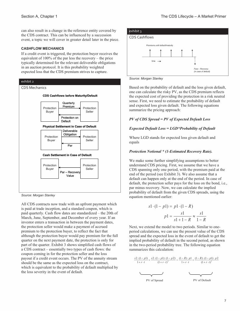
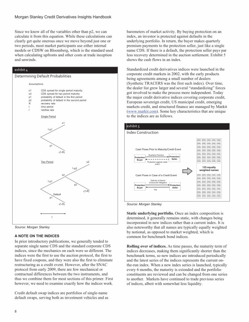
CASHFLOW MECHANICS If a credit event is triggered, the protection buyer receives the equivalent of 100% of the par less the recovery – the price typically determined for the relevant deliverable obligations in an auction protocol. It is this probability weighted expected loss that the CDS premium strives to capture.
exhibit�2�
CDS�Mechanics
Protection Buyer
Protection Seller
Quarterly Premium
Protection on Default
CDS Cashflows before Maturity/Default
Protection Buyer
Protection Seller
DeliverableObligation
Par
Physical Settlement in Case of Default
Protection Buyer
Protection Seller
Par – RecoveryValue
Cash Settlement in Case of Default
Protection Buyer
Protection Seller
Quarterly Premium
Protection on Default
CDS Cashflows before Maturity/Default
Protection Buyer
Protection Seller
DeliverableObligation
Par
Physical Settlement in Case of Default
Protection Buyer
Protection Seller
Par – RecoveryValue
Cash Settlement in Case of Default
Source: Morgan Stanley
All CDS contracts now trade with an upfront payment which is paid at trade inception, and a standard coupon, which is paid quarterly. Cash flow dates are standardized – the 20th of March, June, September, and December of every year. If an investor enters a transaction in between the payment dates, the protection seller would make a payment of accrued premium to the protection buyer, to reflect the fact that although the protection buyer would pay premium for the full quarter on the next payment date, the protection is only for part of the quarter. Exhibit 3 shows simplified cash flows of a CDS contract – essentially two types of cash flows: the coupon coming in for the protection seller and the loss payout if a credit event occurs. The PV of the annuity stream should be the same as the expected loss on the contract, which is equivalent to the probability of default multiplied by the loss severity in the event of default.
exhibit 3
CDS Cashflows
Premiums until default/maturity
time
Face - Recovery(in case of default)
Source: Morgan Stanley
Based on the probability of default and the loss given default, one can calculate the risky PV, as the CDS premium reflects the expected cost of providing the protection in a risk neutral sense. First, we need to estimate the probability of default and expected loss given default. The following equations summarize the pricing approach:
PV of CDS Spread = PV of Expected Default Loss
Expected Default Loss = LGD*Probability of Default
Where LGD stands for expected loss given default and equals
Protection Notional * (1-Estimated Recovery Rate).
We make some further simplifying assumptions to better understand CDS pricing. First, we assume that we have a CDS spanning only one period, with the premium paid at the end of the period (see Exhibit 3). We also assume that a default can happen only at the end of the period. In case of default, the protection seller pays for the loss on the bond, i.e., par minus recovery. Now, we can calculate the implied probability of default from the given CDS spreads, using the equation mentioned earlier:
Rs
Rssp
Rpps
��
���
�����
11
1111
)1(1)11(1
Next, we extend the model to two periods. Similar to one-period calculations, we can use the present value of the CDS spread and the expected loss in the event of default to get the implied probability of default in the second period, as shown in the two-period probability tree. The following equation summarizes this calculation:
22 )1(2)11()1(
11)1(
)1()21()11(2
1)11(2
trppR
trpR
trpps
trps
������
�����
���
�����
����
PV of Spread PV of Default
Morgan Stanley Credit Derivatives Insights Handbook
8
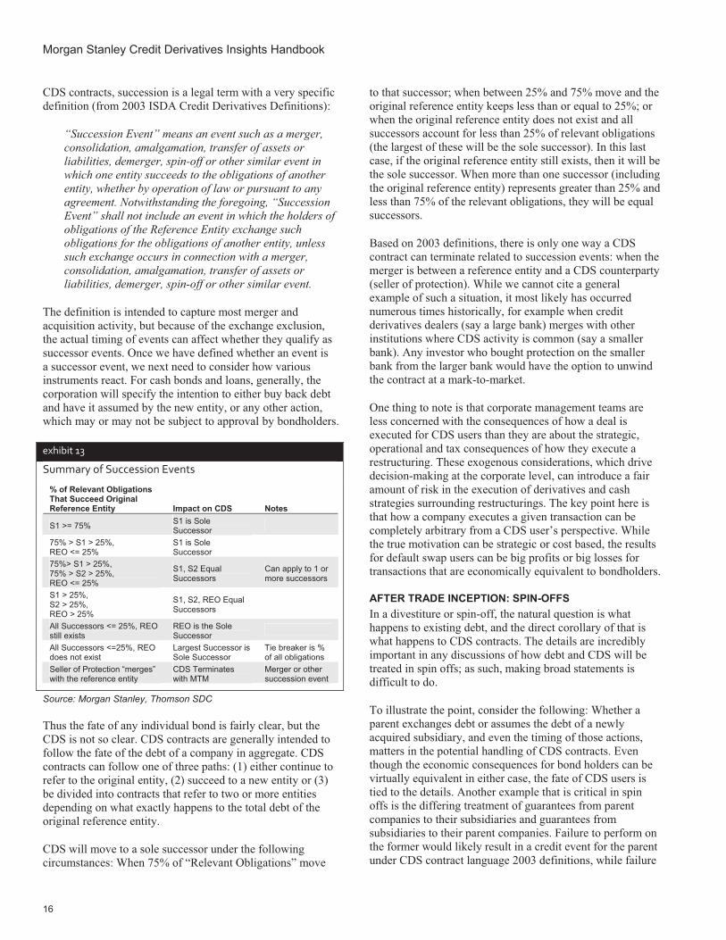
Since we know all of the variables other than p2, we can calculate it from this equation. While these calculations can clearly get quite onerous once we move beyond just one or two periods, most market participants use either internal models or CDSW on Bloomberg, which is the standard used when calculating upfronts and other costs at trade inception and unwinds.
exhibit 4
Determining Default Probabilities Assumptions
s1 CDS spread for single period maturitys2 CDS spread for two period maturityp1 probability of default in the first periodp2 probability of default in the second periodR recovery ratet time periodr riskfree rate
Single Period
s1
1-p1
p1
-(1-R)
Two Period s2
1-p2
s2
1-p1p2
-(1-R)Default
p1
-(1-R)
t
Source: Morgan Stanley
A NOTE ON THE INDICES In prior introductory publications, we generally tended to separate single name CDS and the standard corporate CDS indices, since the mechanics on each were so different. The indices were the first to use the auction protocol, the first to have fixed coupons, and they were also the first to eliminate restructuring as a credit event. However, after the SNAC protocol from early 2009, there are few mechanical or contractual differences between the two instruments, and thus we combine them for most sections of this primer. First however, we need to examine exactly how the indices work.
Credit default swap indices are portfolios of single-name default swaps, serving both as investment vehicles and as
barometers of market activity. By buying protection on an index, an investor is protected against defaults in the underlying portfolio. In return, the buyer makes quarterly premium payments to the protection seller, just like a single name CDS. If there is a default, the protection seller pays par less recovery determined in the auction settlement. Exhibit 5 shows the cash flows in an index.
Standardized credit derivatives indices were launched in the corporate credit markets in 2002, with the early products being agreements among a small number of dealers (Synthetic TRACERS was the first such index). Over time, the dealer list grew larger and several “standardizing” forces got involved to make the process more independent. Today the major credit derivative indices covering corporate credit, European sovereign credit, US municipal credit, emerging markets credit, and structured finance are managed by Markit (www.markit.com). Some key characteristics that are unique to the indices are as follows.
exhibit 5
Index Construction
Delivery of Senior Unsecured Obligation
Par
Cash Flows in Case of a Credit Event
Protection Seller
Quarterly Premium
Protection against credit event
CDS CDS CDS CDS CDS
CDS CDS CDS CDS CDS
CDS CDS CDS CDS CDS
CDS CDS CDS CDS CDS
CDS CDS CDS CDS CDS
CDS CDS CDS CDS CDS
CDS CDS CDS CDS CDS
CDS CDS CDS CDS CDS
CDS CDS CDS CDS CDS
CDS CDS CDS CDS CDS
CDS CDS CDS CDS CDS
CDS CDS CDS CDS CDS
CDS CDS CDS CDS CDS
CDS CDS CDS CDS CDS
125 equally weighted names
Protection Buyer
Protection Buyer
Protection Seller
Cash Flows Prior to Maturity/Credit Event
Source: Morgan Stanley
Static underlying portfolio. Once an index composition is determined, it generally remains static, with changes being incorporated in new indices rather than a current index. It is also noteworthy that all names are typically equally weighted by notional, as opposed to market weighted, which is common for benchmark bond indices.
Rolling over of indices. As time passes, the maturity term of indices decreases, making them significantly shorter than the benchmark terms, so new indices are introduced periodically and the latest series of the indices represents the current on-the-run index. When a new index series is launched, typically every 6 months, the maturity is extended and the portfolio constituents are reviewed and can be changed from one series to another. Markets have continued to trade previous series of indices, albeit with somewhat less liquidity.

Section A, Chapter 1 The CDS Lifecycle – A Market Primer
9
Quoting convention. One thing to note is that in standard quotation, HY, LCDX, Lev-X and HY indices are quoted on a price basis whereas CDX IG, iTraxx Main and XOver, SovX and MCDX are quoted on a spread basis, even though all trade with the upfront plus coupon format.
exhibit 6
Impact of Default on an Index
CDS
CDS CDS CDS CDS
CDS CDS CDS CDS CDS
CDS CDS CDS CDS CDS
CDS CDS CDS CDS CDS
CDS CDS CDS CDS CDS
CDS CDS CDS CDS CDS
CDS CDS CDS CDS CDS
CDS CDS CDS CDS CDS
CDS CDS CDS CDS CDS
CDS CDS CDS CDS CDS
CDS CDS CDS CDS CDS
CDS CDS CDS CDS CDS
CDS CDS CDS CDS CDS
CDS CDS CDS CDS CDS
124 equally weighted names
CDS CDS CDS CDS CDS
CDS CDS CDS CDS CDS
CDS CDS CDS CDS CDS
CDS CDS CDS CDS CDS
CDS CDS CDS CDS CDS
CDS CDS CDS CDS CDS
CDS CDS CDS CDS CDS
CDS CDS CDS CDS CDS
CDS CDS CDS CDS CDS
CDS CDS CDS CDS CDS
CDS CDS CDS CDS CDS
CDS CDS CDS CDS CDS
CDS CDS CDS CDS CDS
CDS CDS CDS CDS CDS
125 equally weighted names
Defaulted name settled
separately
Source: Morgan Stanley
Cash flows upon default. When an underlying single name defaults, it is removed from the index and settled separately. For example, if one of the 125 underlying names in CDX IG were to default, the remaining index would have 124 names and the same deal spread. The 1/125th of the notional would be separated and the protection seller would pay par to the protection buyer in exchange for a deliverable obligation. After a default, the premium payments for the index would be (124/125)*index coupon*original notional. It is important to note that an equal-weighted portfolio of underlying names could now have a different spread, given that each of the underlying names has its own spread level and that, depending on which of the 125 names defaults, the average spread for the remaining 124 names could be different from 124/125 of the original spread.
For the remainder of the primer we will continue to reference single name CDS; however, the mechanics and execution are the same for both the indices and single names.
CONTRACT DEFINITION: CREDIT EVENT TRIGGERS The ultimate value of a CDS contract is derived from the credit events that can trigger it, the bonds and loans that are deliverable upon this event, and their expected recovery. Market sentiment and technicals can greatly influence CDS spreads, but it is important to consider contract language to determine value. CDS contracts have to trigger under a specific type of credit event. Broadly speaking, the most common credit events are bankruptcy, failure-to-pay and restructuring. Other triggers include repudiation/moratorium and obligation acceleration, but these are much less frequent and highly specific to certain types of credit risk.
Based on asset type and geography, a CDS contract may have a combination of the above mentioned types (see Exhibit 7 for the various triggers and classes of debt required to trigger a credit event). The legal and regulatory backdrop in each region, along with differences in the investor base can greatly influence contract language. The vast majority of credit events in the corporate world are bankruptcies, and the CDS contract is now well tested for such events, though the absence of a well-oiled bankruptcy framework makes restructurings more common in Europe and Asia than in the US. One thing to note is that banks do not achieve full capital relief when restructuring is not included in the CDS as a credit event (though this is being discussed with regulators currently and may change). As bank investors are a significant investor base in Europe and Asia, CDS includes restructuring as a credit event in those regions, whereas in North America, corporate CDS contracts do not include restructuring.
Aside from those credit events listed, there are also a few rare instances that can trigger a CDS contract, such as Fannie Mae and Freddie Mac, which triggered the CDS in 2008 after being put into a conservatorship. Though rare, this is relevant for corporates with strong governmental linkages.
For sovereign CDS, bankruptcy does not apply, and instead the credit events are failure to pay, restructuring and repudiation / moratorium, though restructuring is the primary trigger event that predominantly drives valuation. Russia and Ukraine in 1998 would probably have triggered under the repudiation / moratorium clause. There are also several important differences between European EM and Western European sovereigns. First, credit event tests are applicable only to bonds for European EM sovereigns, whereas they are applicable to any borrowed money (including bi-lateral lending agreements) for Western European Sovereigns. Additionally, sovereign lender debt is not applicable in Asia but it is applicable in Europe. Finally, only non-domestic law and non-domestic currency bonds are applicable for European EM sovereigns whereas domestic bonds are also relevant for Western European Sovereigns. See Exhibit 7.
In the municipal market failure-to-pay and restructuring are the only credit events, with the notable omission of bankruptcy. Though some municipalities can file for bankruptcy under U.S. law, they can only file for Chapter 9, and not all municipalities are able to do this according to their individual state constitutions. While the details of this are better left to another report, the important thing to note here is that most bankruptcies would likely include either a failure to pay, a restructuring, or both, and thus would eventually trigger the CDS contract anyway. Municipal restructuring is “old style”, which is different from the restructuring type used in the corporate world (see the following section).

Morgan Stanley Credit Derivatives Insights Handbook
10
CONTRACT DEFINITIONS: CANCELLABILITY IN LCDS There have been some contract changes in the LCDS market in the US recently, bringing some much needed clarity to the market. The first change is that the single name and index markets will now trade with a standard 250bps coupon, with 100bp and 500bp available if needed. The second change is regarding cancellation risk in LCDS. The key concern with the prior LCDS contract was pricing and valuation uncertainty, given the cancellability or early termination feature of underlying loans, which is akin to a credit defaulting with a recovery of 100%.
The old LCDS contract stated that a simple loan refinancing (with another loan) would not lead to a cancellation/early termination event and the contract would still remain outstanding. However, when a company chooses to replace its existing secured debt by bonds, the loan actually gets paid down, which can happen when a company has access to cheaper unsecured financing, often due to a ratings upgrade. In this case, there is no appropriate reference obligation outstanding in the market to be delivered into the LCDS contract, and under the old contract, the LCDS contract could be terminated. Now, the new LCDS contract does not include optional early termination rights, and in the absence of a credit event, if a valid deliverable obligation does not exist, the “orphaned” LCDS will continue to remain outstanding, similar to the unsecured CDS market.
Additionally, there was some confusion in the LCDS contract regarding succession and refinancing events. The concern was that it was sometimes unclear whether new entities first assumed or became liable for the original loans prior to them being repaid, which could cause some LCDS contracts to be orphaned. To avoid this, the definition of succession and refinancing events have been expanded to include the following, according to Markit (www.markit.com):
� Repayment of Relevant Obligations from the proceeds of new loans or bonds from a new entity
� Repayment of Relevant Obligations where the assets securing them have been acquired by proceeds of new loans or bonds from a new entity
� Repayment of Relevant Obligations where the assets securing them subsequently secure new loans or bonds of a new entity
� Amendment or Restructuring where the Relevant Obligations cease to be obligations of the original Reference Entity and another entity becomes a borrower or provides a qualifying affiliate guarantee
� Any other event that has substantially the same effect as the above.
CONTRACT DEFINITION: RESTRUCTURING The most common source of credit event ambiguity stems from restructuring credit events. The ISDA 2003 credit derivatives definitions characterize restructuring credit events
as a reduction in coupon or principal, a deferral of an interest or principal payment, a change in the ranking of priority of payments, or changes to the currency of the interest and principal payments. The currency criteria state that a redenomination of debt into G7 currencies is permitted, OR redenomination into any OECD currency as long as the local-currency long-term debt rating is AAA or higher by S&P, Moody’s, or Fitch. This latter point is important for EMU members with sub-AAA ratings as an event where they leave the EMU and re-denominate their debt into a new local currency would trigger a CDS credit event via restructuring.
There are also additional burdens to prove a restructuring event. Restructuring must be coercive to trigger the CDS – i.e., it must be agreed upon a by a sufficient number of holders before it becomes binding on all the holders. Unless Multiple Holder Obligation is specified as not applicable, the obligation has to be held by at least two-thirds of the investors. Furthermore, restructuring is not applicable if any of the above events has not been the result of deterioration in credit quality. Finally, there are variations to deliverable obligations depending on the type of restructuring clauses. In the case of the corporate restructuring, there are limitations on the maturity of the bond that can be delivered into the contract.
As a result of all these requirements, examples of triggering CDS under the restructuring clause have been few and far between. Xerox was a notable example, and Thomson recently experienced a restructuring, which turned out to be a painful learning experience for market participants. Another recent restructuring example is Aiful, which triggered a restructuring credit event (old R) leading to the first CDS auction in Japan.
Post SNAC, restructuring credit events will now be much rarer, as restructuring was eliminated as a credit event in new corporate contracts in the US. Nonetheless, it is important to understand the various restructuring types and the implications therein for the large legacy market, as well as the specific corners of the market where restructuring is still a credit event. It is conceivable for a CDS credit event to trigger from a restructuring where all the bonds of the reference entity remain outstanding and continue trading based on their interest rate risk.
Old Restructuring. This was the original form of restructuring. Old style restructuring implies that, in the event of a restructuring, bonds of any maturity less than 30 years can be delivered, which can introduce a significant amount of interest rate risk into a CDS contract upon a restructuring credit event (i.e., a 30 year fixed-rate bond could trade at a significant discount to par in a high interest rate environment). This is particularly important given that the municipal market tends to be long in duration.
Modified Restructuring and ModMod Restructuring. In 2002 the restructuring of a Xerox obligation brought to light long duration interest rate risk, driving the introduction of

Section A, Chapter 1 The CDS Lifecycle – A Market Primer
11
modR for the US and modmodR for Europe to the 2003 ISDA definitions for corporate CDS. As a result of this, many CDS contracts introduced maturity limitations for restructuring credit events.
We have tried to provide a brief overview of the various elements of the contract, but there is a wealth of material on ISDA and Mark-it that we recommend.
exhibit 7
Overview of Standard Credit Events for Various CDS Contracts
Bankruptcy Failure to Pay
Failure to Pay
(Grace Period Appl.)
Obligation Acceleration
Repudiation/ Moratorium
Restructuring (Old R)
Restructuring Maturity
Limitation and Fully Transferable
Obligation (Mod R)
Modified Restructuring
Maturity Limit and Conditionally Transferable Obligation
(Mod Mod R)
Multiple Holder Obligation Required?
(If Restructuring) Asia Sovereign N Y N N Y Y N N Y Singapore Sovereign N Y N N Y Y N N Y Latin America Sovereign N N Y Y Y Y N N N Emerging European & Middle Eastern Sovereign N N Y Y Y Y N N N Western European Sovereign N Y N N Y Y N N Y Japan Sovereign N Y N N Y Y N N N Australia Sovereign N Y N N Y N Y N Y New Zealand Sovereign N Y N N Y N Y N Y U.S. Municipal Full Faith And Credit N Y N N N Y N N N U.S. Municipal General Fund N Y N N N Y N N N U.S. Municipal Revenue N Y N N N Y N N N North American Corporate Y Y N N N N N N Y European Corporate Y Y N N N N N Y Y Australia Corporate Y Y N N N N Y N Y New Zealand Corporate Y Y N N N N Y N Y Japan Corporate Y Y N N N Y N N N Singapore Corporate Y Y N N N Y N N Y Asia Corporate Y Y N N N Y N N Y Subordinated European Insurance Corporate Y Y N N N Y N N Y Emerging European Corporate LPN Y N Y N Y Y N N Y/N Emerging European Corporate Y N Y N Y Y N N Y/N "Latin America Corporate B" Y N Y Y Y Y N N N "Latin America Corporate BL" Y N Y Y Y Y N N Y
Overview of Obligation Characteristics* to Trigger a Credit Event
Obligation Category
Not Subordinated
Not Sovereign
Lender
Not Domestic Currency
Not Domestic
Law
Not Domestic Issuance
Standard Specified Curr. & Domest
Currency
Full Faith & Credit Oblig.
Liab.
General Fund Oblig.
Liab. Revenue
Oblig. Liab.Asia Sovereign Bond /Loan Y Y Y Y Y N N N N Singapore Sovereign Bond /Loan Y Y N N N Y N N N Latin America Sovereign Bond Y N Y Y Y N N N N Emerging European & Middle Eastern
Sov. Bond Y N Y Y Y N N N N
Western European Sovereign BM N N N N N N N N N Japan Sovereign BM N N N N N N N N N Australia Sovereign BM N N N N N N N N N New Zealand Sovereign BM N N N N N N N N N U.S. Municipal Full Faith And Credit BM Y N N N N N Y N N U.S. Municipal General Fund BM Y N N N N N N Y N U.S. Municipal Revenue BM Y N N N N N N N Y North American Corporate BM N N N N N N N N N European Corporate BM N N N N N N N N N Australia Corporate BM N N N N N N N N N New Zealand Corporate BM N N N N N N N N N Japan Corporate BM Y N N N N N N N N Singapore Corporate Bond /Loan Y Y N N N Y N N N Asia Corporate Bond /Loan Y Y Y Y Y N N N N Subordinated European Insurance Corp. BM N N N N N N N N N Emerging European Corporate LPN Bond /Loan Y N Y Y Y N N N N Emerging European Corporate Bond /Loan Y N Y Y Y N N N N "Latin America Corporate B" Bond Y N Y Y Y N N N N "Latin America Corporate BL" Bond /Loan Y Y Y Y Y N N N N
Note: BM – Borrowed Money. Obligation characteristics* refers to the obligations on which credit event tests are applicable. Source: ISDA, Morgan Stanley Research

Morgan Stanley Credit Derivatives Insights Handbook
12
exhibit 8
Overview of Deliverable Obligations for Various CDS Contracts
Obligation Category
Not Subordinated
Not Sov. Lender
Not Dom-estic Law
Not Domestic Issuance
Max Maturity 30 yrs
Assign-able Loan
Consent Required
Loan
Speci-fied
Curr-ency
Std Specified Curr. &
Domestic Curr.
Specified Curr. &
Domestic Curr.
Std Speci-
fied Curr-
encies Latin America Sovereign Bond Y N Y Y N N N Y N N N Emerging European & Middle Eastern Sov. Bond Y N Y Y N N N Y N N N Western European Sovereign Bond /Loan N N N N Y Y Y Y N N N
Japan Sovereign Bond /Loan N N N N Y Y Y Y N N N
Australia Sovereign Bond /Loan Y N N N Y Y Y N Y N N
New Zealand Sovereign Bond /Loan Y N N N Y Y Y N Y N N
Asia Sovereign Bond /Loan Y Y Y Y Y Y N Y N N N
Singapore Sovereign Bond /Loan Y Y N N Y Y N N N Y N
U.S. Municipal Full Faith And Credit Bond /Loan Y N N N Y Y Y N N N Y
U.S. Municipal General Fund Bond /Loan Y N N N Y Y Y N N N Y
U.S. Municipal Revenue Bond /Loan Y N N N Y Y Y N N N Y
North American Corporate Bond /Loan Y N N N Y Y Y Y N N N
European Corporate Bond /Loan Y N N N Y Y Y Y N N N
Australia Corporate Bond /Loan Y N N N Y Y Y N Y N N
New Zealand Corporate Bond /Loan Y N N N Y Y Y N Y N N
Japan Corporate Bond /Loan Y N N N Y Y Y Y N N N
Singapore Corporate Bond /Loan Y Y N N Y Y N N Y N N
Asia Corporate Bond /Loan Y Y Y Y Y Y N Y N N N Subordinated European Insurance
Corp. Bond /Loan Y N N N Y Y Y Y N N N
Emerging European Corporate LPN Bond /Loan Y N Y Y N Y Y Y N N N
Emerging European Corporate Bond /Loan Y N Y Y N Y Y Y N N N
"Latin America Corporate B" Bond Y N Y Y N N N Y N N N
"Latin America Corporate BL" Bond /Loan Y Y Y Y N Y Y Y N N N Note: BM – Borrowed Money. Source: ISDA, Morgan Stanley Research
CONTRACT DEFINITION: DELIVERABLE OBLIGATIONS Another important factor in determining CDS valuation is deliverable obligations. Common considerations for determining deliverability are the currency, maturity, subordination, governing law and market of issuance.
First we address maturity. Corporate CDS in Japan and Asia, most OECD sovereigns, and municipal CDS (as we mentioned above) in the US use “Old R” restructuring, under which maturities of up to 30 years are deliverable if a restructuring credit event occurs, allowing interest rate levels to determine the cheapest-to-deliver bond if bonds do not accelerate (i.e., become due immediately as they would in a corporate bankruptcy).
Type of debt is another interesting point to note when discussing deliverability. For instance, in Europe, only non-domestic debt is deliverable for EM sovereigns unlike Western European sovereigns. Additionally, only bonds are deliverable in European EM and Latin American sovereigns, whereas both bonds and loans are deliverable for Western European and Asian sovereigns. These are all things to keep in mind when evaluating the cheapest to deliver option, which ultimately impacts the value of the CDS.
An important point to consider is the language of the underlying bonds. Bonds issued over different periods tend to
have variation in the clauses as well – this is particularly true in the sovereign space. For example the absence of cross-default provisions in the bond language makes a significant difference to the way bonds across the curve trade relative to the CDS in times of distress.
TRADE INITIATION: FIXED COUPONS REDUCE RISKS Prior to SNAC in 2009, most CDS contracts traded on an all running basis, with the exception of a few very distressed names. Thus if an investor were to buy protection on a name that was quoted at 110bp, the trade would simply have a coupon of 110bp. During times of credit distress, however, this became an issue as unwinding a CDS contract is complicated when the strike price is very far out of the money, a theme we have highlighted in numerous pieces (see Credit Volatility – the Unintended Consequences from April 1, 2005 and LCDS, After the Trade from June 1, 2007). Investors who wanted to unwind a trade done without a fixed coupon often found large penalties associated with the unwind due to the mismatched coupon streams. With a fixed coupon this legacy annuity risk is significantly reduced, as any difference in risk premium is paid in the form of an upfront payment. To illustrate this concept, we offer the following example.
Consider an example, where an investor purchased 5-year protection on credit “X” at 100bp in January 2008 and then

Section A, Chapter 1 The CDS Lifecycle – A Market Primer
13
subsequently elected to monetize the trade in March 2009 when spreads to the same maturity widened to 1,000bp. To monetize this widening, the investor could do one of two things. The first would be to sell protection at a strike of 1,000bp, and then hold two offsetting trades, one that is paying 100bps and another that is receiving 1,000bps. In this scenario, the investor would be hedged from a default risk perspective, however, now has IO risk in this credit in the event of default.
Why? The key here is the uncertainty of the total cash flows and P&L for the investor depending on the whether or not a credit event is triggered. The investor now receives 900bp (the difference between these two coupon streams) until maturity or a credit event. If a credit event were to occur, both contracts would trigger, the default loss settlement of the two contracts would offset each other, and both coupon streams would stop. Thus the 900bps the investor had been receiving on a default “riskless” basis is now gone. Thus while the default settlement is hedged, the coupon stream is still exposed to default risk. In this example, if the default occurs one year later, the investor would have received $0.9mm on a $10mm position (900bp * 10mm). If the default is in four years, the investor would have received $3.6mm in total cash flow from the coupons.
To eliminate this risk, the investor can instead unwind the original 100bp swap and receive the PV of the 900bps difference between the 100bps coupon and the 1,000bps of credit risk the swap is now worth to monetize the P&L immediately. The investor unwinds the original swap struck at 100bp and receives an upfront amount of $2.9mm, which is the PV of the 900bp stream assuming a remaining duration of 3.2. In addition to having hedged the default risk on the reference entity, the investor has now eliminated the credit risk inherent in the risky coupon (as well as counterparty exposure, which is a separate issue). From the investor’s perspective, the trade is completely closed and monetized.
However the uncertainty in cash flows is not eliminated, but instead transferred to the dealer. Why? Because the dealer now has to hedge the position with the market standard contract. In this example, where floating coupons are market standard, the dealer would have paid out $2.9mm today to buy protection at 100bp running from the investor, but can only sell protection to another investor on the now current running coupon – in this case 1,000bp. If there is an immediate default, the dealer loses the $2.9mm paid to the investor but has not received any of the 1,000bp coupon from the protection sold. The dealer has effectively become exposed to the jump risk that the investor just got rid of. In the past, the dealer could buy short dated protection (say 1-year protection) to hedge these early default scenarios, but would most likely pass this additional cost, or at least some fraction of it, on to the investor who was unwinding the trade. This resulted in different spreads shown depending on
whether the investor was unwinding an off-market coupon or putting on a new trade.
Thus prior to the advent of standardized fixed coupons the dealer incurred additional risk and costs when using a non-standard fixed strike CDS arising from a) the cost of funding the upfront payment to be paid to the investor and b) hedging the annuity risk from an early default by buying jump protection. With the fixed strike contracts, each of these legs becomes more fungible and can be hedged immediately with offsetting contracts that have the same coupon and maturity and would involve the transfer of the same upfront amount. This is also important in light of the development of a central clearinghouse, as a clearinghouse would face the same issues when presented with different floating strike contracts from different counterparties.
TRADE INITIATION: FIXED COUPON SENSITIVITY Following SNAC standardization in 2009, most CDS contracts now trade with a fixed coupon, with the exception of municipal CDS in the US, though that may change in the future. The implication of using fixed coupons is that instead of paying the full CDS premium each year, an upfront payment will be exchanged based on the difference between the coupon and the ‘spread’ or ‘premium’.
The most common coupon strikes are 100bps and 500bps for most CDS contracts around the world. The exact coupon for a name will be a function of the current spread level, the historic spread range and legacy exposures. Three exceptions are a) some European corporates which also have 25bp and 1,000bp available, although the latter is unlikely to be used much; b) Japan corporate and sovereign CDS which have 25bp also available; c) Western European sovereign CDS which has only 25 and 100bp as a choice (and not 500bp) and d) US LCDS contracts that as of 2010 will trade with a standard fixed coupon of 250bp (though 100bp and 500bp will also be available for tight and wide credits, respectively).
exhibit 9
Coupon Standards around the World
CDS 25 100 250 500 1000 Asia Sovereign & Corporate Y Y Latin America Corporate & Sovereign Y Y Emerging European & Middle Eastern Sovereign Y Y Western European Sovereign Y Y Japan Corporate & Sovereign Y Y Y Australia, New Zealand Corporate & Sovereign Y Y North America LCDS Y North American Corporate & Sovereign CDS Y Y European Corporate Y Y Y Y
Source: Morgan Stanley
As we highlighted before, the coupons were standardized to reduce jump-to-default risk inherent in having extremely out-of-the-money coupons when trying to unwind that resulted in legacy annuity risk. However, other considerations remain,

Morgan Stanley Credit Derivatives Insights Handbook
14
even in light of making all coupons conform to one of 4 strikes. One of the bigger issues we are seeing today even with standardized coupons is the impact of CDS curve structure on upfront pricing at different coupon strike levels.
To illustrate, say we have a 5-year CDS with a par spread of 250bps. The convention is to use Bloomberg CDSW with a flat curve. With coupon of 100bp, the upfront payment on this will be 6.7%. However, since many market participants do not use a flat curve in their internal risk systems, the par spread will be slightly different when used with a full maturity curve to achieve the same upfront levels. In our example the equivalent level is 244bp. If we then change the coupon to, for instance, 500bps using the same upward sloping curve shape as before, we get an upfront level of 11.9%. Finally, we use this upfront to get an equivalent flat curve par spread, and we see that to get this same 11.9% using a flat curve, we have a par spread of 237bps, a difference of 13bp from where we began.
How is this possible? We have several different par spreads for what should be equivalent risk. The answer lies in the default risk implied by the curve shape. It is intuitive that a positively sloped curve is less risky than a flat curve with the same 5-year point, so an upward sloping curve structure will imply lower default probabilities and thus a higher probability of the fixed coupon actually being paid. When we change the coupon to be higher, i.e., from 100 to 500bp, more of the premium paid to the seller of protection is at risk. So to have equivalently risky contracts, a lower “par spread” is used to compensate for the higher running coupon. Consequently, we are seeing that different strike contracts and different curve shapes produce different par spreads, even when the fixed coupon and upfront remain the same.
Another way to look at this is instead to look at the way upfronts change when curve shape changes. In Exhibit 10, we show that given a CDS with a par spread of 250 basis points, the upfront amounts will change pretty significantly based on the type of curve shape used – even though all are using the same 5-year spread of 250bps.
exhibit 10
Curve Shape Affects Upfront Pricing
Curve Shape 5-year CDS
Spread Fixed Coupon
of 100bps Fixed Coupon
of 500bp Upward Sloping 250bp 7.0% -11.7%Flat 250bp 6.7% -11.2% Inverted 250bp 6.6% -11.0%
Source: Morgan Stanley
TRADE INITIATION: COMMON METRICS AND MODELS When trading CDS, an investor goes long risk (sells protection) and earns a “spread” to compensate for the probability of default of the underlying entity in a risk neutral framework. As a result, the present value of all these
incremental cash flows should equal the present value of expected losses. The probability of default of an entity is determined using market CDS spreads across the maturity spectrum.
exhibit 11
Bloomberg CDSW
Spread DeltaFixed Coupon
Par Spread
Upfront Payment
Source: Bloomberg, Morgan Stanley
The PV01 of a CDS contract (referred to as risky duration) is simply the present value of 1bp of the cash flow at every coupon payment date. It can also be interpreted as the mark-to market sensitivity of expected losses in a CDS contract to a 1bp parallel shift in the spread term structure of the underlying entity. In contrast to the calculation for the duration of a bond or risk-free interest rate swap, the discount factors for CDS duration are higher, as they have a survival probability term associated with them. This additional discount factor reduces the present value of cash flows, and consequently the risky duration for similar cash flows in CDS vs. less risky assets.
The duration of a CDS contract depends on the shape of the maturity structure as it directly impacts survival probability. For example, given two CDS contracts with the same term structure from 0 to 5 years, the duration would be lower for the contract with a flatter curve beyond the 5-year point, since it implies a higher default probability and thus a lower PV.
Spread delta or DV01 is a more pertinent metric to look at today, given the advent of fixed coupons. Unlike duration, which is the sensitivity of the contract to a change in expected loss assumptions, the spread delta captures just the mark-to-market sensitivity of the contract to a 1bp parallel shift in the credit curve. Thus we get this equation:
Upfront payment = (Par spread – Fixed Coupon)*PV01
DV01 is essentially the first derivative of the upfront payment with respect to par spread. The above equation

Section A, Chapter 1 The CDS Lifecycle – A Market Primer
15
shows that when a contract trades at par, the spread delta is the same as duration. However, as the coupon differs from the par spread, the change in upfront payment also depends on the change in PV01 with respect to spread (i.e., convexity).
TRADE INITIATION: CLEARINGHOUSES Mandatory clearing might be a major component of the regulatory reform, at least as far as the credit markets are concerned, with a primary objective of maximizing clearing of derivatives trades in the market. Today, the clearinghouse is legging in on certain types of transactions, starting with dealer to dealer trades on the most liquid products and expanding from there. These trades will eventually include all liquid index products and most single names. As of publication we are already clearing indices and some single names, and the list of eligible trades for the clearinghouse continues to grow.
While the counterparty type will be an important factor in whether or not a trade needs to be cleared or exchange-traded, the trade type may also be considered. For instance, some highly bespoke trades may not be required (or able) to go through a clearing house or derivative exchange. If these trades, or others, do not go through a clearing house, there will likely be reporting requirements imposed. Furthermore, who determines what is required to be cleared is being discussed and right now the CFTC (and SEC when appropriate) are most likely to have the authority to determine what is clearable.
exhibit 12
Central Counterparty Mechanics
Bank
Bank
Bank
Bank
Bank
Bank
Bank
Bank
Bank
Bank
CCP
Bank
Bank
Bank
Bank
Bank
Bank
Bank
Bank
Bank
Bank
Bank
Bank
CCP
Bank
Bank
Source: Morgan Stanley
AFTER THE TRADE: DEALING WITH SUCCESSION EVENTS A number of corporate and financing structure decisions also have an influence on CDS. Event risks to keep in mind are corporate refinancings, business restructurings, asset sales,
divestitures, M&A and LBOs. While most of what we focus on in this section deals with the 2003 ISDA definitions, we highlight that succession events were one of the many topics covered by SNAC provisions of 2009, specifically regarding look-back dates for determining credit events and succession events. Prior to SNAC, the effective and succession event dates were fixed dates (at the time of trade date plus one), meaning that, in theory, a credit event could be declared anytime between the effective date and the maturity of the CDS contract. One of the issues surrounding the prior standard is that offsetting trades or hedges could have different windows for succession event determination, introducing a certain amount of incremental basis risk. Under the new contract, this long period of potential succession event declaration is reduced to no more than 90 days prior.
While there are numerous corporate situations where the timing of debt exchanges and the ultimate par value of debt that moves between entities determines successor behavior in CDS, we endeavor to provide some basic rules of thumb regarding the impact of succession events (or the lack thereof) on CDS contracts, based on the 2003 ISDA definitions. Here are some of the broader themes:
� When there are corporate successions, CDS contracts follow the debt of a company, rather than equity value, revenues or corporate structure. A corporate succession must result in a “Succession Event,” under the 2003 ISDA definitions, for CDS to change, although CDS can be implicitly affected without such an event.
� The key difference between bonds and CDS in the event of succession is that CDS can be formulaically split, while bonds, by definition, have to go one direction or another (or get taken out).
� It is rare for CDS to be terminated as a result of corporate succession. The only situation where it can happen is where the party to the corporate action is also the protection seller, in which case a “Termination Event” occurs. Even then, it results in a mark-to-market unwind at the option of the protection buyer.
� A debt exchange that is not in connection with a merger (or other terms of a “Succession Event”) will not qualify as a “Succession Event.” As such, there could be situations where no obligations are left to be deliverable into the CDS, although debt issued in the future could be.
� One company guaranteeing the debt of another company (say, after buying its stock) does not qualify as a “Succession Event.” If the debt is assumed by the parent company and released by the original obligor, then it is a “Succession Event.”
For bond purposes, succession really has more to do with making the credit risk of the instruments of one issuer economically similar to the instruments of another issuer. For
Morgan Stanley Credit Derivatives Insights Handbook
16
CDS contracts, succession is a legal term with a very specific definition (from 2003 ISDA Credit Derivatives Definitions):
“Succession Event” means an event such as a merger, consolidation, amalgamation, transfer of assets or liabilities, demerger, spin-off or other similar event in which one entity succeeds to the obligations of another entity, whether by operation of law or pursuant to any agreement. Notwithstanding the foregoing, “Succession Event” shall not include an event in which the holders of obligations of the Reference Entity exchange such obligations for the obligations of another entity, unless such exchange occurs in connection with a merger, consolidation, amalgamation, transfer of assets or liabilities, demerger, spin-off or other similar event.
The definition is intended to capture most merger and acquisition activity, but because of the exchange exclusion, the actual timing of events can affect whether they qualify as successor events. Once we have defined whether an event is a successor event, we next need to consider how various instruments react. For cash bonds and loans, generally, the corporation will specify the intention to either buy back debt and have it assumed by the new entity, or any other action, which may or may not be subject to approval by bondholders.
exhibit 13
Summary of Succession Events
% of Relevant Obligations That Succeed Original Reference Entity Impact on CDS Notes
S1 >= 75% S1 is Sole Successor
75% > S1 > 25%, REO <= 25%
S1 is Sole Successor
75%> S1 > 25%, 75% > S2 > 25%, REO <= 25%
S1, S2 Equal Successors
Can apply to 1 or more successors
S1 > 25%, S2 > 25%, REO > 25%
S1, S2, REO Equal Successors
All Successors <= 25%, REO still exists
REO is the Sole Successor
All Successors <=25%, REO does not exist
Largest Successor is Sole Successor
Tie breaker is % of all obligations
Seller of Protection “merges” with the reference entity
CDS Terminates with MTM
Merger or other succession event
Source: Morgan Stanley, Thomson SDC
Thus the fate of any individual bond is fairly clear, but the CDS is not so clear. CDS contracts are generally intended to follow the fate of the debt of a company in aggregate. CDS contracts can follow one of three paths: (1) either continue to refer to the original entity, (2) succeed to a new entity or (3) be divided into contracts that refer to two or more entities depending on what exactly happens to the total debt of the original reference entity.
CDS will move to a sole successor under the following circumstances: When 75% of “Relevant Obligations” move
to that successor; when between 25% and 75% move and the original reference entity keeps less than or equal to 25%; or when the original reference entity does not exist and all successors account for less than 25% of relevant obligations (the largest of these will be the sole successor). In this last case, if the original reference entity still exists, then it will be the sole successor. When more than one successor (including the original reference entity) represents greater than 25% and less than 75% of the relevant obligations, they will be equal successors.
Based on 2003 definitions, there is only one way a CDS contract can terminate related to succession events: when the merger is between a reference entity and a CDS counterparty (seller of protection). While we cannot cite a general example of such a situation, it most likely has occurred numerous times historically, for example when credit derivatives dealers (say a large bank) merges with other institutions where CDS activity is common (say a smaller bank). Any investor who bought protection on the smaller bank from the larger bank would have the option to unwind the contract at a mark-to-market.
One thing to note is that corporate management teams are less concerned with the consequences of how a deal is executed for CDS users than they are about the strategic, operational and tax consequences of how they execute a restructuring. These exogenous considerations, which drive decision-making at the corporate level, can introduce a fair amount of risk in the execution of derivatives and cash strategies surrounding restructurings. The key point here is that how a company executes a given transaction can be completely arbitrary from a CDS user’s perspective. While the true motivation can be strategic or cost based, the results for default swap users can be big profits or big losses for transactions that are economically equivalent to bondholders.
AFTER TRADE INCEPTION: SPIN-OFFS In a divestiture or spin-off, the natural question is what happens to existing debt, and the direct corollary of that is what happens to CDS contracts. The details are incredibly important in any discussions of how debt and CDS will be treated in spin offs; as such, making broad statements is difficult to do.
To illustrate the point, consider the following: Whether a parent exchanges debt or assumes the debt of a newly acquired subsidiary, and even the timing of those actions, matters in the potential handling of CDS contracts. Even though the economic consequences for bond holders can be virtually equivalent in either case, the fate of CDS users is tied to the details. Another example that is critical in spin offs is the differing treatment of guarantees from parent companies to their subsidiaries and guarantees from subsidiaries to their parent companies. Failure to perform on the former would likely result in a credit event for the parent under CDS contract language 2003 definitions, while failure

Section A, Chapter 1 The CDS Lifecycle – A Market Primer
17
to perform on the latter would likely not result in a credit event for the subsidiary (it is likely that only downstream guarantees matter; we note that this behavior could be different in Europe).
DEFAULT SETTLEMENT: THE AUCTION PROCESS In the past, credit events on single name CDS were settled either entirely in cash or entirely physically (with bonds or loans) and the standardized index tranches had a hybrid cash/physical settlement mechanism. Both the sheer volume of outstanding CDS contracts on the indices and the demand for index tranches to be fungible after a credit event created huge demand in the marketplace for a standardized settlement process, which is now the standard for all CDS settlement today, on assets from single name CDS to indices to tranches on indices. Starting in 2005 with the Collins & Aikman default, numerous investors have participated in industry-wide settlements. The benefits of an auction are manifold, but the primary benefit is that it is operationally efficient to use a common recovery for all trades to eliminate basis risk between products.
As of April 23, 2010, the International Swaps and Derivatives Association (ISDA) had published CDS protocols for over 70 defaulted entities (see Exhibit 14), and the resulting auctions (including both senior and subordinated debt) were administered by Markit Partners and CreditEx. The protocols are available on the ISDA website, www.isda.org, and details of the auctions are available on www.creditfixings.com. Just as in succession events, the SNAC protocol added look-back provisions for determining a credit event, and today, the credit event has to have happened within the last 60 days to be eligible for settlement.
The objective of the auction is to concentrate trading in the bond(s) during a short window of time to arrive at a recovery. To initiate this process, market participants submit a request to the Determination Committee (DC) with information on a potential credit event. After the SNAC Big Bang protocol, this must be within two months of the credit event, as now all contracts have a fixed 60-day lookback period in which to declare a credit event, similar to the succession event requirements. The DC then decides whether the credit event has occurred and what type. It also decides whether an auction will be conducted (in case the outstanding CDS in a name is very small, no auction may be conducted). There are some additional complexities for trades with restructuring, in which case an auction may need to be conducted for different maturity buckets to take into account maturity limitations under restructuring. Now that the market standard is to use contracts without restructuring triggers, this will be less common going forward, however there are still a number of legacy trades with restructuring on them (see http://www.isda.org/companies/thomson/docs/Restructuring-CE-FAQs.pdf).
There are some additional provisions that are specific to the “Small Bang” protocol in Europe:
� The DC publishes an auction protocol which outlines the maturity buckets for which an auction will be conducted, and the deliverables for the same.
� Unlike other Credit Events, where a DC resolves that a Restructuring Credit Event has occurred, this does not automatically trigger the CDS. Both counterparties have the right to trigger their transaction but this remains a manual process and not automatic.
� Both the buyer and the seller have the option, but not the obligation to trigger the CDS. When the final list of deliverable obligations is published, depending on the notifying party, the seller of protection has 2 business days and the buyer of protection has 5 business days to trigger the transaction.
The process determines one recovery rate (or one for each maturity bucket in the case of a restructuring event), which is used to cash settle the credit event in all single name CDS contracts, index transactions and determine losses (for equity tranches) and subordination levels (for non-equity tranches) for tranches in all covered indices. We encourage readers to visit the ISDA website (www.isda.org) to get current information on the methodology, as our summary should in no way be considered a complete or accurate description of either past or future protocols.
To illustrate the auction methodology, we take the example of Masonite from December 2008 for a relatively simple bankruptcy auction. The auction involves a two-stage process. In stage 1, the dealers establish indicative markets by quoting both a bid and offer for the bonds in a pre-defined size as well as physical settlement requests – i.e., requests for buying or selling bonds through the auction. In the case of Masonite, dealers submitted a bid-offer in 2.5MM size. We also see that there is a demand to buy bonds through the auction (18MM notional of bonds).

Morgan Stanley Credit Derivatives Insights Handbook
18
exhibit 14
Selected ISDA Auctions
Recovery (%)
Credit Event Credit
Event Date Auction
Date SnrSec Senior Unsec Sub
Collins and Aikman 5/17/2005 6/14/2005 43.625 6.375Northwest Airlines 9/14/2005 10/11/2005 28.000 Delta Airlines 9/14/2005 10/11/2005 18.000 Delphi 10/10/2005 11/4/2005 63.375 Calpine 12/20/2005 1/17/2006 19.125 Dana 3/3/2006 3/31/2006 75.000 Dura 10/30/2006 11/28/2006 24.125 3.500 Movie Gallery 9/15/2007 10/23/2007 91.500 Quebecor 1/21/2008 2/19/2008 41.250 Tembec 9/4/2008 10/2/2008 83.000 Fannie Mae 9/7/2008 10/6/2008 91.510 99.90 Freddie Mac 9/7/2008 10/6/2008 94.000 98.00 Lehman Brothers 9/15/2008 10/10/2008 8.625 Washington Mutual 9/27/2008 10/23/2008 57.000 Landsbanki 10/8/2008 11/4/2008 1.250 0.125 Glitnir 10/8/2008 11/5/2008 3.000 0.125 Kaupthing Bank 10/9/2008 11/6/2008 6.625 2.375 Masonite 11/14/2008 12/9/2008 52.500 Hawaiian Telecom 12/1/2008 12/17/2008 40.125 Tribune 12/8/2008 1/6/2009 23.750 1.500 Ecuador 12/18/2008 1/14/2009 31.375 Lyondell 1/7/2009 2/3/2009 20.750 15.500 Millenium 1/7/2009 2/3/2009 7.125 Equistar 1/7/2009 2/3/2009 27.500 Nortel Ltd 1/14/2009 2/10/2009 6.500 Nortel Corp 1/14/2009 2/10/2009 12.000 Smurfit-Stone 1/26/2009 2/19/2009 65.375 8.875 Aleris 2/13/2009 3/9/2009 8.000 Station Casinos 3/4/2009 3/31/2009 32.000 Chemtura 3/19/2009 4/14/2009 15.000 Great Lakes 3/20/2009 4/14/2009 18.250 Rouse 3/20/2009 4/15/2009 29.250 LyondellBasell 3/23/2009 4/16/2009 2.000 Charter 3/27/2009 4/21/2009 78.000 2.375 Abitibi 3/27/2009 4/17/2009 3.250 Capmark 3/30/2009 4/22/2009 23.375 Idearc 3/31/2009 4/23/2009 38.500 1.750 Bowater 4/16/2009 5/12/2009 15.000 Syncora 5/1/2009 5/27/2009 15.000 JSC BTA Bank 5/1/2009 6/10/2009 10.250 HLI Operating Co. 5/13/2009 6/9/2009 9.500 Dex Media East 5/18/2009 6/24/2009 77.250 R.H. Donnelley Inc. 5/18/2009 6/24/2009 78.125 Dex Media West 5/18/2009 6/24/2009 82.875 R.H. Donnelley 5/18/2009 6/11/2009 4.875 Georgia Gulf 5/19/2009 6/10/2009 83.000 JSC Alliance Bank 5/19/2009 6/18/2009 16.750 Visteon 5/28/2009 6/23/2009 39.000 3.000 General Motors 6/1/2009 6/12/2009 97.500 12.500 Six Flags 6/13/2009 7/9/2009 96.125 14.000 Lear 7/6/2009 7/21/2009 66.000 38.500 Bradford & Bingley 7/9/2009 7/30/2009 94.625 5.000 Thomson 8/12/2009 10/22/2009 65.125 NJSC Naftogaz 10/14/2009 12/16/2009 83.500 Metro-Goldwyn- 10/19/2009 11/10/2009 58.500 CIT 11/2/2009 11/20/2009 68.125 Hellas II 11/19/2009 12/15/2009 1.375 Thomson 12/1/2009 12/10/2009 77.750 FGIC 12/3/2009 1/7/2010 26.000 Cemex 12/14/2009 2/18/2010 97.000 Aiful 12/30/2009 3/2/2010 33.875 Japan Airlines Corp 1/21/2010 4/22/2010 20.000 Ambac Assurance 3/26/2010 TBD TBD
Source: Morgan Stanley. As of April 23, 2010
From the bid-offers we arrive at the market mid-points. In Exhibit 15 we sort the bids in descending order and offers in ascending order separately and eliminate tradable markets.
exhibit 15
Masonite Auction Stage 1- Dealer Inside Markets and Physical Settlement Requests
Inside Markets Physical Settlement Requests Dealer Bid Offer Bid/Offer Size Merrill Lynch 47.5 50.5 Offer 0.0 Goldman Sachs 48.0 51.0 Bid 0.0 Barclays Bank 48.5 51.5 Offer 10.0 Citigroup 48.6 51.6 Offer 2.5 JP Morgan Chase 49.5 52.5 Offer 0.0 Credit Suisse 50.0 53.0 Bid 5.5 UBS 50.0 53.0 Offer 0.0 Bank of America 51.0 54.0 Offer 0.0 Deutsche Bank 52.0 55.0 Bid 5.0 Morgan Stanley 52.0 55.0 Bid 20.0 Total Bid 18.0MM
Source: Markit
Of the remaining 8 bids/offers, we take an average of the best half (rounded up) of the bids and offers ending up with 50.125 as our inside bid and 52.156 as our inside offer. The inside market mid-point (IMM) is the average of the above two rounded to the nearest 1/8th, ending up at 51.125 for Masonite. There is a penalty amount that dealers have to pay for being offside on the market – in this case, the ML and GS offers are below, considering there is open interest of 18MM to buy bonds. The dealers have to pay the quotation times the difference between the IMM and the offer, so in this particular case this would be $15,625 and $ 3,125 (2.5MM * (offer – IMM)), as penalty, respectively.
exhibit 16
Masonite Auction – Arriving at Market Mid-Point
Dealer Bid Offer Dealer Deutsche Bank 52.000 50.500 Merrill Lynch Morgan Stanley 52.000 51.000 Goldman Sachs Bank of America 51.000 51.500 Barclays Bank Credit Suisse 50.000 51.625 Citigroup UBS 50.000 52.500 JP Morgan Chase JP Morgan Chase 49.500 53.000 Credit Suisse Citigroup 48.625 53.000 UBS Barclays Bank 48.500 54.000 Bank of America Goldman Sachs 48.000 55.000 Deutsche Bank Merrill Lynch 47.500 55.000 Morgan Stanley Average 50.125 52.156
Source: Markit
After stage 1 of the auction, market participants get a few hours to evaluate the information from stage 1 and put in bids or offers to close the open interest. In this example, investors put in their offers of the bonds to close the net 18MM bid for bonds. The bids/offers for the pre-defined size (in this case the offers) from the stage1 is carried forward to stage 2.
So, in the case of Masonite, the dealers are deemed to have offered 2.5MM of bonds at the offer levels in stage 1. Then, the administrator will determine the final price from the auction by matching market orders until the open interest is

Section A, Chapter 1 The CDS Lifecycle – A Market Primer
19
cleared. In the case of Masonite, 52.5 was the clearing price (Ex 17).
In the case of a mod R or mod mod R restructuring event, the auction is conducted by collapsing bonds and outstanding CDS into several buckets ensuring that the maturity limitation restriction we highlighted earlier is not violated. From a protection buyer perspective, the "Limitation Date" means the first of March 20, June 20, September 20 or December 20 in any year to occur on or immediately following the date that is one of the following numbers of years after the restructuring date: 2.5 years (the "2.5-year Limitation Date"), 5 years (the "5-year Limitation Date"), 7.5 years, 10 years, 12.5 years, 15 years, 20 years or 30 years, as applicable. For each bucket, the restructuring maturity limitation we discussed earlier applies. An auction is conducted for buckets with sufficient CDS outstanding. In the Thomson restructuring event in August 2009, the auction was conducted for three different buckets 2.5-year, 5-year and 7.5-year, reflecting the predominance of CDS trading in the maturities less than 10-years, as well as the deliverables available.
exhibit 17
Masonite Auction – Arriving at Market Mid-Point
Dealer Offer Size Barclays 50.125* 5 Merrill Lynch ** 51.125* 2.5 Goldman Sachs ** 51.125* 2.5 Barclays ** 51.5* 2.5 Citigroup ** 51.625* 2.5 Goldman Sachs 52* 2.5 JP Morgan Chase** 52.5^ 2.5 JP Morgan Chase 52.5^ 5 Credit Suisse 52.625 4 Credit Suisse ** 53 2.5 UBS ** 53 2.5 Bank of America 53.5 2.5 Bank of America** 54 2.5 Bank of America 54 2.5 Credit Suisse 54 4 Merrill Lynch 54.75 2.5 Deutsche Bank AG** 55 2.5 Morgan Stanley ** 55 2.5 Credit Suisse 55 3.5 Bank of America 55 2.5 JP Morgan Chase 55.5 5 JP Morgan Chase 56 5 JP Morgan Chase 57 3 Barclays 65 5
Note: ** Limit Orders that were derived from inside markets. * Limit Orders that were filled. ^ Limit Orders that were partially filled.
Source: Markit

Morgan Stanley Credit Derivatives Insights Handbook
20
Chapter 2
The Credit Volatility Culture – An Options Primer May 7, 2010
Sivan Mahadevan Phanikiran Naraparaju Ashley Musfeldt
From an investment and portfolio management perspective, credit as an asset class has evolved quite a bit over the past few years. Prior to the financial crisis, much of the risk management effort in credit was focused on default risk, but not necessarily market risk, which is why the CDS market developed quite rapidly while a corresponding options market did not. Since about 2003, there has been some demand for hedging credit market risk as well, and this demand accelerated at the peak of the credit crisis, leaving us a market today that is broader and deeper with much room for growth.
Many core credit investors are able to hold healthy credit instruments on an accrual basis, and as such are more concerned about default risk than market risk. But the investor base and credit culture have changed dramatically over the past few years, as many non-financial institutions have entered the market as buyers of credit risk. For this community, credit is no different than equity in that market volatility is something to be concerned about. Furthermore, CDS usage among both financial and non-financial institutions is generally on a mark-to-market basis, so investors who may use CDS to hedge default risk in corporate bonds and loans (held on an accrual basis) may still introduce credit volatility into their portfolios. As such, credit volatility has become important for a large group of investors, and the credit crisis underscored that premise.
A credit options (also known as credit swaptions) market started as early as 2003, when options on the then-standard US corporate CDS indices began. Pre-crisis, popularity was larger in Europe where liquidity focused on the iTraxx XOver index first (high yield) and eventually iTraxx Main (investment grade) as the crisis intensified. But the market’s largest growth began in 2008, in the depths of the credit and financial crisis. Today, the credit options market is fairly active on index products, with options trading on iTraxx XOver, iTraxx Main, CDX IG and HY indices with good liquidity, and SOVX, iTraxx Senior financials and options on the Asian indices also trading in periods of stress.
We have a few years of experience now in credit options, encompassing credit markets before, during and after the credit crisis. Although credit has normalized relative to the crisis, we expect to see continued development of an options culture in credit as the lessons learned from the crisis are secular in our view. Typical investment strategies can be bullish or bearish directionally, and long or short market volatility as well.
Much like equities, we expect to see credit investors lean toward two classes of strategies: downside hedging and income generation. As such, we think the equity market options culture is a good framework for credit investors to understand, keeping in mind that the underlying return potential of credit can differ significantly from that of equities. Credit, especially investment grade credit, is more skewed to the downside at normal spread levels. As such, we would expect the option skew to follow a similar pattern in that there should be more demand for OTM puts or payers than OTM calls or receivers. But despite a more normal distribution of returns in equities, we still see this style of skew in option pricing, owing to the market’s demand for hedging and overwriting.
In contrast to considerable hedging flows, a culture of overwriting and generating yield through credit options strategies is less developed – mainly because most credit investors are naturally long risk assets anyway and standalone returns had been attractive coming out of the crisis. This may change if we see risk premiums compress further and indices start trading in a range-bound environment. Many investors look at different ways to monetize a lower volatility environment, and we remind investors that the culture of callable bonds is quite well established in credit; hence, there is precedent for option-related income generation strategies.
In this primer, we trace the evolution of the credit options market through the crisis, examine lessons learned and discuss how this market might develop. We also include a basic primer, describe options nomenclature and common option strategies, and conclude with a discussion of option sensitivities (i.e., the Greeks) and pricing models. We note that all options discussed in this primer trade OTC.
CREDIT VOLATILITY IN CONTEXT Volatility is a measure of market uncertainty, and data and analysis of the path of volatility in the equity markets demonstrates that the level of uncertainty has a strong cyclical component, rising during periods of weak growth or recession while staying low during periods of normal growth. This is of course intuitive: uncertainty should be higher when we are “outside” the normal market periods and lower when “inside.” And since periods of positive economic growth generally occur more frequently than do recessions, we can justify higher levels of uncertainty and market volatility in cyclically weak periods (see Volatility in a Recovery – Views for a Turning Cycle, September 16, 2009).
Given this cyclical link, volatility across markets has a tendency to be well correlated over long periods of time, especially when considering broad market measures of such

Section A, Chapter 2 The Credit Volatility Culture – An Options Primer
21
volatility (see Exhibit 1). And given that this volatility can be negatively correlated to the returns of risky assets, many market participants consider volatility to be an asset class unto itself, with important diversification properties.
Indeed through the crisis, we have seen equity investors fishing for credit hedges and credit investors chasing equity hedges, in an attempt to source cheaper or more effective hedges. There are certainly many things the credit options market can learn from the far more mature equity options market. However, there are also many elements that are quite unique to credit options.
Given that much valuation in credit is done with spreads instead of prices, credit options for IG and iTraxx Main are quoted as spread options, which is similar to the rates markets. Spread options are calculated as the annualized average daily log changes in spreads. Price options, on the other hand, are used for CDX HY, and this type of option quotation is more analogous to the equities and FX markets. For most of our purposes here, we have used price volatility for ease of understanding and comparison.
Most of the activity in the credit options market is relatively short-dated compared to the other markets. Credit index options have standard expiries that correspond to the quarterly CDS payment months, with other expiries gaining liquidity intermittently. For instance, in May of a particular year, the June, September, and potentially even December expiries should trade, with potential liquidity in some May and July expiries as well, and the expiry date is the third Wednesday of the month for credit options. The options that are traded in the market today tend to have expiries that are generally less than one year (3m and 6m options tend to be the most liquid). Credit options investors and dealers prefer options on the OTR index for better liquidity in the underlying and ease of risk management, though occasionally the legacy series will trade, particularly around roll dates.
In Exhibit 1, we illustrate credit volatility compared to FX, and highlight that XOver and HY volatility has traded in ranges that are similar to FX volatility (EURUSD or JPYUSD), though the range of volatility in HY has been wider than FX. Part of the reason for the more frequent and higher spikes in HY vol is the asymmetric nature of the credit asset class.
exhibit 1
Price Volatility Across Asset Classes
3M Volatility (%)
0%
5%
10%
15%
20%
25%
30%
Sep-06 Mar-07 Sep-07 Mar-08 Sep-08 Mar-09 Sep-09 Mar-100%
10%
20%
30%
40%
50%
60%
EURUSD 3M10Y Xover SPX (RHS)
3M Volatility (%)
0%
5%
10%
15%
20%
25%
Sep-06 Mar-07 Sep-07 Mar-08 Sep-08 Mar-09 Sep-09 Mar-10
iTraxx Main 3M5Y 3M10Y EURUSD
Source: Morgan Stanley Research, Bloomberg
For IG vol (we use iTraxx Main for the longer history on the European side), the closest comparable volatility metric is 5yr swaption vol. As seen in Exhibit 1, during the crisis IG vol reached a peak similar to that of swaption vol (around 10%), but also healed quite dramatically relative to swaption vol.
The other aspect that is different for credit is the carry, which is quite high for credit relative to the yield. HY credit, with a 5% coupon, has the largest “dividend” among the assets, compared to dividend yields of 2% or less for US equities and less than 4% for European equities or carry differentials in currency. Much of the return at tighter spread levels for credit is generated through carry and hence overwriting strategies make a lot of sense in credit.

Morgan Stanley Credit Derivatives Insights Handbook
22
exhibit 2
State of the Credit Options Market
Coupon/ 3M Implied Vol 3M Realized Vol 3m Vol 6m Implied
Vol
Dividend Current High Jun-07 Current High Jun-07 Carry Current Credit iTraxx Main 1.0% 4.9% 10.1% 0.6% 2.7% 6.3% 0.4% 2.2% 4.5% CDX IG 1.0% 4.6% 11.2% n/a 2.8% 8.9% 0.6% 1.8% 4.5% iTraxx XOver 5.0% 14.6% 24.6% 2.6% 9.0% 16.5% 4.6% 5.6% n/a CDX HY 5.0% 18.1% n/a n/a 12.0% 28.4% 6.3% 6.1% n/a Equities S&P 500 2.1% 26.7% 63.1% 12.8% 14.2% 72.3% 9.8% 12.5% 26.8% Russell 2000 1.3% 32.8% 68.9% 18.0% 17.3% 79.3% 13.6% 15.5% 33.6% Eurostoxx 4.2% 30.3% 61.8% 15.0% 18.4% 65.9% 13.7% 11.9% 29.2% DAX 3.4% 25.2% 61.1% 16.2% 15.8% 63.7% 14.3% 9.4% 25.2% FTSE 3.9% 23.4% 60.7% 13.0% 13.0% 62.9% 11.1% 10.4% 23.8% FX EURUSD 0.3% 15.2% 15.2% 24.5% 10.0% 10.0% 22.2% 5.2% 15.1% GBPUSD 0.3% 14.8% 14.8% 25.5% 10.9% 10.9% 22.7% 3.9% 14.5% USDJPY 0.3% 15.3% 15.3% 33.5% 13.8% 13.8% 20.4% 1.5% 15.3% Rates USD 5yr Swap 2.4% 6.1% 10.8% 2.7% 4.3% 10.8% 2.9% 1.8% 6.2% USD 10yr Swap 3.4% 10.8% 18.7% 4.6% 7.8% 18.6% 4.1% 3.0% 11.0%
Note: All Vols are Price Vols. For credit and rates, it is the spread vol * spot * duration. Source: Morgan Stanley Research, Bloomberg.
CREDIT VOLATILITY INTUITION As we discussed above, credit spread volatility (implied by index option pricing) is a much different concept than the price volatility that most investors are used to observing in the equity and FX markets, and is instead similar to the lognormal volatility in the rates market. Here, to compare volatility over time or across different markets, investors look at normalized volatility, which is calculated as the lognormal vol multiplied by the level of rates. We must also consider duration, an additional factor in the credit market used to convert normalized volatility into price volatility.
To illustrate, we offer the following example. Say implied volatility on a particular index with a spread of 200bp is 60%. This means that annualized volatility on the index is 60%, which would be equivalent to a daily implied volatility of about 3.72% (60% divided by square root of 260 business days in a year). This is equivalent to a daily spread move of 7.4bp (3.72% times the index spread of 200bp). This, in turn, translates into a standard deviation of daily price moves of about 0.33% (7.4bp times an approximate duration of 4.5). This is equivalent to an annualized price volatility of 5.3% (0.33% times the square root of 260 business days). In Exhibit 2, we show price volatility of a variety of asset classes.
Credit is unique among asset classes in that the upside/downside is very skewed: there is a very high likelihood of a small upside and a very small likelihood of a large downside. This has implications for the volatility carry, skew and the term structure of credit. The out-of-the-money (OTM) and asymmetric nature of credit compared to the equity or FX markets makes it prone to volatility spikes in periods of stress, superimposed over long periods of exceptionally low volatility. Credit spreads have been quite volatile and fat tailed, with IG realized spread volatility ranging from 10–100% over the last several years.
Due to this asymmetric nature, the volatility carry (i.e., the gap between implied and realized volatility) can be substantial in credit. Implied volatility has been consistently higher than realized volatility for the credit indices historically, as investors are willing to pay a premium, keeping in mind these volatility spikes. This is particularly true for IG options – the low absolute cost attracts options buyers. Conversely, sellers of volatility generally need a higher premium over realized in IG options. HY volatility is likely to appeal to sellers of vol to a larger extent due to better absolute premiums.

Section A, Chapter 2 The Credit Volatility Culture – An Options Primer
23
exhibit 3
Volatility Carry
0%
5%
10%
15%
20%
25%
30%
Feb-07 Aug-07 Feb-08 Aug-08 Feb-09 Aug-09 Feb-10-8%
-4%
0%
4%
8%
12%
16%
20%
Vol Carry (RH)3M Realized3M Implied
Source: Morgan Stanley
exhibit 4
iTraxx Term Structure
50%
60%
70%
80%
90%
100%
110%
120%
130%
Jan-08 Jul-08 Jan-09 Jul-09 Jan-10-40%
-30%
-20%
-10%
0%
10%
20%
30%
40%
3m-6m Curve 3 M Vol
Source: Morgan Stanley
Another implication of the asymmetric nature of credit is that shorter-dated volatility tends to price in a premium to longer-dated volatility in calmer markets, reflecting the risk of periods of very high volatility. The gap between one-month and three-month volatility tends to widen significantly in periods of stress. Whenever this term discount for volatility disappears, it represents a period of relatively low risk premiums embedded in the options market, and in these markets we think that a strategy of buying short-dated options could perform well.
Not only do shorter-dated options trade at a volatility premium, there is also a significant element of skew embedded in OTM options. In particular, there is a strong technical demand for options to buy protection at the OTM strikes. Volatility tends to spike substantially when spreads widen, because even investors who are long credit risk use these OTM options as disaster insurance. Option skews have generally ranged between 10–15% for various options.
exhibit 5
Option Skew for XOver Options
6%8%
10%12%14%16%18%
83% 101% 113% 131% 155%
Strike (as a % of Spot)
Impl
ied
Vola
tility
today 1 week back 1 month back
Source: Morgan Stanley
HEDGING STRATEGIES WITH CREDIT OPTIONS Even before the crisis, hedging was the dominant source of flows in the options market. Loan books, counterparty desks, and structured credit books were the predominant users of options for hedging. The most common strategy was buying OTM payers (puts). Post crisis, setting up a systematic hedging strategy has been one of the most common topics of discussion among investors. The ideal hedging strategies vary based on the scenario being hedged for, the level of volatility and skew, the term structure and the hedging budget.
One strategy is to hedge for smaller tail scenarios, which we define as 30bp wider on IG credit and 150bp wider on HY. In an environment in which realized volatility has been declining, term structures and skew are both steep. One common strategy to hedge for this type of scenario is to buy out-of-the-money puts outright. Put spreads are another effective way to position for such a move, and we have seen investors implement this strategy as well.
To hedge for larger tail scenarios, in which IG credit is 60bp+ wider and HY credit 300bp+ wider, longer-dated strategies might offer better value. Buying long-dated OTM puts is an effective strategy when the indices are trading at tight levels and volatility is relatively low.
To hedge for a market widening (either small or large tail) in periods when implied volatility is fairly high, investors try to reduce the cost of buying puts or put spreads by selling a call to monetize the high implied volatility. The resulting strategies – risk reversals (buy OTM put, sell OTM call) or put spread collars (buy put spread and sell OTM call) – have relatively low exposure to changes in implied volatility (or even short volatility in some scenarios) while retaining a directionally bearish exposure.
To compare the different type of strategies, we calculate the max downside and upside for each strategy based on the bear and bull case for the index. See an illustrative example in

Morgan Stanley Credit Derivatives Insights Handbook
24
showing the risk/reward of various strategies to hedge a small-tail scenario. Historically a reward to risk ratio higher than 2.5x is desirable and a ratio in 4-5x context for a realistic tail scenario could be considered very good.
YIELD GENERATION STRATEGIES WITH OPTIONS The use of the options market for yield generation has been a relatively recent development. In environments where carry takes on a stronger role in driving credit returns, but volatility remains elevated, overwriting – i.e., selling call options against long positions as a way to enhance yield – should appeal to investors. Such strategies are common in equities, but less common in credit. In Exhibit 6, we show how much of an impact overwriting can have on realized yields in HY options as an illustration. For example, say an investor can sell a 4-month OTM call on CDX HY that earns an annualized premium of 270bp when CDX HY is at 550bp. Thus the premium is almost half the carry of the CDX HY in this particular example. This is effectively like buying a
callable bond with a “call price” of 100.8 (the breakeven level) which is nearly a 3-point premium to the price of 97.9.
exhibit 6
Overwriting in CDX HY and XOver CDX HY
Expiry Spread Yield Breakeven Yield Breakeven Yield Breakeven1m 5.6% 8.8% 99.4 3.4% 100.1 2m 5.6% 6.1% 99.8 3.8% 100.5 2.1% 101.3 4m 5.6% 3.9% 100.2 2.7% 100.8 1.7% 101.5 6m 5.6% 2.5% 100.4 1.8% 101.0 1.3% 101.7
XoverExpiry Spread Yield Breakeven Yield Breakeven Yield Breakeven1m 4.4% 7.8% 103.2 1.7% 104.04m 4.4% 3.9% 104.0 2.7% 104.8 1.7% 105.5
Call @ 101
Call @ 102.9 Call @ 104.0 Call @ 105.0
Call @ 99 Call @ 100
Assuming CDX HY Index Price is 97.9. XOver Index Price is 102.3. Breakeven level is effectively the “call price” of the package. Prices are indicative. Source: Morgan Stanley Research
exhibit 7
Bloomberg CDS Option Pricer
CDS option specifications include:
� The underlying CDS contract, usually 5-year maturity.
� Strike level specified for the spread (typical range 90–130% of current spread).
� Typical option expiry (liquid maturities extend from one month up to six months).
� The options are European and exercisable only on expiry date and into underlying CDS (physical or cash settlement).
� Options are quoted in bp upfront, i.e., the price of the option is paid upfront. No other cash flows are exchanged until the expiry.
Source: Morgan Stanley
PRICING MODELS AND INDEX OPTIONS CDS options can in theory be on any CDS instrument, although in practice the focus in the market is on CDS indices. A simple model based on Black’s formula typically suffices for the pricing of a European option on a single-name CDS. However, index options and single-name options have a key difference in the case of credit events. The option buyer in an index contract continues to retain the option to buy or sell protection on all the remaining names in the event of a default of one of the names. The convention for single-name CDS options is to trade with knock-out, i.e., the single-name option
extinguishes upon a credit event. Thus, adjustments may be necessary when applying the same model to index options. The market generally uses various adaptations of the Black model. A simple model is publicly available on Bloomberg (type <CDSO>) for basic pricing and analyzing sensitivities. See Exhibit 7 for more on CDSO.
The convention in the market is for CDS index options to trade “without knock-out” which means that even if a credit does default, the performance of the rest of the index constituents is also important when determining whether or not to exercise

Section A, Chapter 2 The Credit Volatility Culture – An Options Primer
25
the option. To illustrate, assume an investor has bought deep OTM payers with a strike of 325bp on a 100-name index trading at 200bp. In a scenario where a default occurs with a 40% recovery, the defaulted name is worth 0.6% in P&L (or approximately 15bp in spread terms) for the index, and spreads on the remaining names widen 100bp on average. In this scenario, the net P&L is not enough to make the exercise attractive. Post exercise, the buyer of protection can monetize the default by settling the credit event.
The spread dispersion and number of credits within the index also matter. The pricing of single-name vs. index options has a significant difference, particularly for the OTM payers. In the case of a XOver credit (which has 45 names), single-name OTM payers can be 10-20% more valuable than an identical index option, depending on the strike and the volatility levels due to the default P&L. However, beyond a point, increasing the size of the index does not have a large impact on the pricing of options — for example, increasing the size of the XOver index beyond 50 names has little effect on the price.
Bottom line, the buyer of an index payer option benefits from the implicit protection that is in the option. As such, the cost of a payer option will include the cost of protection for the term of the option. This cost of protection will actually vary depending on the strike, as the protection is less valuable the more out-of-the-money the strike is. Receiver options will not include this implicit cost of protection as recoveries are generally expected to be below par, so there will always be a difference between the full cost of a receiver option and a payer option (over and above what put-call parity would imply).
OPTION CHARACTERISTICS AND GREEKS Some of the common metrics used to measure and manage risk of an option position are:
Delta: Delta is the ratio of the change in the price of the option to that of the market value of the underlying index. This varies from 60% for in-the-money payers to 30% for the more OTM payers, although it depends on the spread level of the underlying index. Delta (of OTM options) is higher for longer maturities compared to shorter maturities.
Gamma: Gamma, or spread convexity, is the change in delta for a 1bp change in the CDS curve. In a higher volatility environment, option gamma falls and eventually becomes unattractive vis-à-vis simple delta exposures. Shorter-dated at-the-money options have the highest gamma.
Vega: Vega is the change in the value of the option for a 1% change in volatility. The vega of an option increases as volatility levels rise. The vega of longer-dated options is higher than shorter-dated options. The vega of the option can contribute significantly to the P&L of the option.
Theta: Theta, or time decay, is the change in value of the option one day closer to expiry. An option with higher
convexity and sensitivity characteristics tends to have higher theta. While the theta of the longer-dated ATM and OTM options is largely similar, that of shorter-dated options drops dramatically as the option goes out of the money.
A typical trader run specifies the maturity, strike, vol and index level used for exchange of deltas. In Exhibit 8, we show the sensitivities for a typical HY run on 3-month and 6-month options.
exhibit 8
Payer Option Greeks Expiry Strike (%) Vol Mid Delta Gamma Theta Vega3m 375 85% 69% 343 2,995 7 (2,030) 1,6783m 400 91% 71% 284 2,710 9 (2,245) 2,0413m 450 102% 75% 192 2,113 11 (2,448) 2,4293m 500 113% 79% 130 1,590 11 (2,385) 2,4263m 550 125% 83% 91 1,185 9 (2,177) 2,2103m 600 136% 85% 61 865 8 (1,852) 1,895 6m 375 85% 62% 468 2,928 5 (1,442) 2,8086m 400 91% 62% 411 2,755 6 (1,485) 3,2066m 450 102% 64% 321 2,375 7 (1,538) 3,7956m 500 113% 66% 252 2,011 7 (1,527) 4,0726m 550 125% 66% 192 1,673 7 (1,437) 4,0986m 600 136% 68% 153 1,396 7 (1,350) 3,954 Note: Greeks calculated on 10MM notional position in the option. Source: Morgan Stanley
exhibit 9
Option Greeks
-
10
20
30
40
50
60
70
80
50 58 65 73 80 88 95 103 110 118 125
Option Strike
Gam
m
3m, Vol @ 70%
3m, Vol @ 90%
6m, Vol @ 70%
6m, Vol @ 90%
-
100
200
300
400
500
600
700
800
900
50 58 65 73 80 88 95 103 110 118 125
Option Strike
Vega
3m, Vol @ 70%
3m, Vol @ 90%
6m, Vol @ 70%
6m, Vol @ 90%
Source: Morgan Stanley

Morgan Stanley Credit Derivatives Insights Handbook
26
OPTION BUILDING BLOCKS Credit options are fairly simple instruments, and even though credit and equity volatility have stronger, more direct fundamental linkages, the lingo is probably more analogous to rates options. At the most fundamental level, credit options give the holder the right to enter into a certain credit default swap at a certain time in the future. We discuss the basic option types and strategies in specific detail in this section (all exhibits show P&L of option strategies for changes in underlying spread, assuming a 10MM notional). As in equities, two basic option types form the building blocks for more complex strategies:
Payer (Put): An investor can buy (or sell) a ‘payer’ option, which is simply an option to buy protection at a fixed spread level on a certain notional at a fixed point in the future. Credit payer options are similar to payer options in interest rates wherein the investor hopes to benefit from wider spreads. They are analogous to equity put options in that the investor is buying (or selling) the right to short risk in the market, in this case by buying (or selling) the right to buy protection.
exhibit 10
Payer Option
Trade P&L
55 60 65 70 75 80 85 90 95 100 105 110 115
Index Spread Level (bp)
Buy Payer
Source: Morgan Stanley
A payer option whose strike level is wider than the index level is referred to as an out-of-the-money (OTM) payer. A payer option whose strike level is the same as the index level is referred to as an at-the-money (ATM) payer. A payer option whose strike level is lower than the index spread level is referred to as an in-the-money (ITM) payer.
Receiver (Call): An investor can also buy (or sell) a ‘receiver’ option, which is an option to sell protection at a fixed spread level on a certain notional at a fixed point in the future. Credit receiver options are similar to receiver options in interest rates wherein the investor hopes to benefit from tighter spreads. They are analogous to equity call options in that the investor is buying (or selling) the right to go long risk in the market, in this case by buying (or selling) the right to sell protection.
exhibit 11
Receiver Option
Trade P&L
50 55 60 65 70 75 80 85 90 95 100 105 110
Index Spread Level (bp)
Buy Receiver
Source: Morgan Stanley
A receiver option whose strike level is lower than the index level is referred to as an out-of-the-money (OTM) payer. A receiver option whose strike level is the same as the index level is referred to as an at-the-money (ATM) payer. A receiver option whose strike level is wider than the index spread level is referred to as an in-the-money (ITM) payer.
Using these two basic option types, we review some of the standard option combinations used to express different views on directionality and volatility of spreads. We have classified these strategies into:
� expressing directionally bullish views
� expressing directionally bearish views
� expressing long volatility views (typically negative carry trades)
� expressing short volatility views (typically income generating)

Section A, Chapter 2 The Credit Volatility Culture – An Options Primer
27
exhibit 12
Directional Option Strategies
Market View (Delta)
Volatility (Vega)
Convexity (Gamma)
Time Decay (Theta) Upside Downside
Buy Payer Bearish Long Long Hurts Position No cap Capped Payer Spread Bearish Neutral Neutral Neutral Capped Capped Sell Receiver Bearish Short Short Helps Position Capped No cap Covered Short Bearish Short Short Helps Position Capped No cap Bear Risk Reversal Bearish Neutral Neutral Neutral No cap No cap Buy Receiver Bullish Long Long Hurts Position No cap Capped Bull Spread Bullish Neutral Neutral Neutral Capped Capped Buy Write Bullish Short Short Helps Position Capped No cap Sell Payer Bullish Short Short Helps Position Capped No cap Bull Risk Reversal Bullish Neutral Neutral Neutral No cap No cap
Volatility Strategies
Market View (Delta)
Volatility (Vega)
Convexity (Gamma)
Time Decay (Theta) Upside Downside
Buy ATM Straddle Neutral Long Long Hurts Position No cap Capped Buy Strangle Neutral Long Long Hurts Position No cap Capped Short Butterfly Neutral Long Long Hurts Position Capped Capped Short Condor Neutral Long Long Hurts Position Capped Capped Cost-neutral Spreads Neutral/Bearish Long Long Hurts Position No cap Capped Long Butterfly Neutral Short Short Helps Position Capped Capped Sell ATM Straddle Neutral Short Short Helps Position Capped No cap Sell Strangle Neutral Short Short Helps Position Capped No cap Long Condor Neutral Short Short Helps Position Capped Capped Ladder Neutral/Bearish Short Short Helps Position Capped No cap
Source: Morgan Stanley
DIRECTIONALLY BULLISH STRATEGIES The primary issue that options veterans have with buying receivers outright to express a bullish view is that volatility generally declines when markets rally. As a result, a buyer of receivers does not get to monetize the full impact of making the right call on the direction of the index (gamma and vega working at cross-purposes). Thus investors look for strategies that take the sting out of a potential decline in volatility or even aim to benefit from a drop. Common strategies investors use to express a directionally bullish view include (1) buying receivers (calls) outright; (2) buying receiver spreads (call spreads); (3) buying 1x2 receiver spreads (buy 1 ATM receiver and sell two further OTM receiver spreads); and (4) bullish risk reversals (buy OTM call and sell OTM put).
Bull Spreads (Receiver Spreads): Spread trades are constructed by buying and selling the receivers but at different strike levels. A receiver spread is constructed by buying a receiver and selling a more OTM receiver. Receiver spreads (RS) express a bullish directional view but cap both the upside and downside relative to being long the index. Receiver spreads have relatively small exposure to changes in implied volatility, as the option positions are offsetting. Consequently, RS can be considered a more defensive trade compared to buying receivers outright.
exhibit 13
Receiver Spread
Trade P&L
60 65 70 75 80 85 90 100
Index Spread Level (bp)
Buy ATM Receiver Sell OTM Receiver Receiver Spread
Source: Morgan Stanley
Buy a 1x2 Receiver Spread: 1x2 receiver spread trades involve buying an ATM receiver and selling twice the notional on an OTM receiver. In this trade, the investor is betting on a modest tightening of spreads but is exposed if indices tighten too far. The benefit to this trade is that the downside is reduced compared to the receivers or receiver spreads if spreads actually end up widening. 1x2 receiver spreads are short volatility and short gamma if there is considerable time to maturity. So the value on the 1x2 RS accretes over time and benefits from time decay. As a tighter spread environment in credit is generally accompanied by a

Morgan Stanley Credit Derivatives Insights Handbook
28
lower volatility environment, some of the short gamma position is offset by positive P&L from a decline in volatility.
exhibit 14
Buy 1x2 Receiver Spread
Trade P&L
55 60 65 70 75 80 85 90 95 100
Index Spread Level (bp)
Buy ATM Receiver Sell 2x OTM Receiver 1x2 Receiver Spread
Source: Morgan Stanley
Buy Bullish Risk Reversals: Bullish risk reversals involve buying an OTM receiver and selling a deep OTM payer to finance. Although the opposite trade (bearish risk reversal) is the more popular counterpart, the bullish RR could be one way of getting around the problem of declining volatility in a rallying market. This trade is better suited for an environment with elevated spreads, limited downside for credit but an uncertain upside.
exhibit 15
Bullish Risk Reversal
Trade P&L
55 60 65 70 75 80 85 90 95 100 105 110
Index Spread Level (bp)
Buy ATM Receiver Sell OTM Payer Bullish Risk Reversal
Source: Morgan Stanley
DIRECTIONALLY BEARISH STRATEGIES Due to the tendency of vol to spike in periods of market stress, the combined impact of the index move and the increase in volatility makes payers very popular, as gamma and vega work in tandem. Nevertheless, other strategies are useful in reducing volatility exposure and/or reducing cost, especially if the timing of sell-off is uncertain and the intensity of a sell-off is expected to be modest. Also in some
cases, volatility spikes may be expected to be unsustainable. Some of the common strategies investors use to express a directionally bearish view include (1) buying payers (puts) outright both with or without delta; (2) buying payer spreads (put spreads); (3) selling 1x2 receiver spreads (sell 1 ATM payer and buy two further OTM payer spreads); (4) bearish risk reversals (sell OTM call and buy OTM put); and (5) put spread collars (sell OTM call and buy OTM put spread).
Bear Spreads (payer spreads): Spread trades are constructed by buying and selling the same type of option but at different strike levels. A payer spread (PS) is constructed by buying a payer and selling a more OTM payer. PS express a bearish directional view but cap both the upside and downside relative to being outright short and are amongst the most common trades in the credit options world. They are particularly useful when volatility levels are high and outright payers are expensive. They are also popular if there is uncertainty regarding the timing of a widening or the expectation of a more modest widening.
exhibit 16
Payer Spread
Trade P&L
65 70 75 80 85 90 95 100 105 110 115 120
Index Spread Level (bp)
Buy ATM Payer Sell OTM Payer Payer Spread
Source: Morgan Stanley
Bearish risk reversal: Bearish risk reversals involve buying an OTM payer and selling an OTM receiver to finance it. Bearish RR are also quite popular as they play to the theme of declining volatility in a rallying market and vice versa, which cushions the MTM if spreads rally. Bearish RR are long gamma in a sell-off and short gamma in a rally and have relatively muted volatility exposure.

Section A, Chapter 2 The Credit Volatility Culture – An Options Primer
29
exhibit 17
Bearish Risk Reversal
Trade P&L
55 60 65 70 75 80 85 90 95 100 105 110
Index Spread Level (bp)
Buy ATM Receiver Sell OTM Payer Bearish Risk Reversal
Source: Morgan Stanley
Payer spread collar: A payer spread collar (PSC) is constructed by buying a payer spread and selling an OTM receiver to further reduce the cost of playing a sell-off in spreads. PSC are less expensive than outright payer spreads but are short gamma and volatility if spreads tighten substantially. If spreads remain range-bound, this is a much cheaper trade than buying payers or payer spreads outright.
exhibit 18
Payer Spread Collar
Trade P&L
60 65 70 75 80 85 90 95 100 105 110 115 120
Index Spread Level (bp)
Buy Payer Spread Sell OTM Receiver Payer Spread
Source: Morgan Stanley
1x2 payer spreads: 1x2 payer spread trades involve selling an ATM payer and buying twice the notional on an OTM payer. Selling 1x2 PS was the ideal trade coming into the crisis when spreads were tight, remained range-bound for a long-period, and implied volatility was very low. This trade is long volatility and convexity, which loses potency over time. The long gamma and convexity in a sell-off and minimal downside in a rally makes 1x2 PS attractive as a MTM hedge, but investors holding this strategy to expiry are really betting on an extreme sell-off if things do go bad and in fact suffer the most downside if spreads widen only modestly.
exhibit 19
Sell 1x2 Payer Spread
Trade P&L
70 75 80 85 90 95 100 105 110 115
Index Spread Level (bp)
Sell ATM Payer Buy 2x OTM Payer 1x2 Payer Spread
Source: Morgan Stanley
LONG VOLATILITY STRATEGIES Long volatility strategies are typically negative carry trades – as implied volatility typically trades at a premium to realized volatility. These strategies therefore suffer with the passage of time to varying degree. Some common strategies used to express a bullish view on volatility (or big out of the range moves) include (1) buying a payer or receiver with delta; (2) buying straddles (buy put and call with the same strike); (3) buying strangles (buying OTM payers and OTM receivers); (4) selling 1x2 payer spreads (sell 1 ATM payer and buy 2x OTM payers); and (5) bearish risk reversals (sell an OTM receiver and buy an OTM payer).
Straddle: A straddle payoff is created by buying a payer and a receiver with the same strike price and expiry. Depending on the strike levels, straddles can be a play on volatility or bets on both the direction of any future price change and its magnitude. While at-the-money straddles struck around the futures price have low deltas, making those more of a volatility play, far-from-the-money straddles have high deltas and represent bets on the level of the underlying spread as well.
exhibit 20
Straddle
Trade P&L
50 55 60 65 70 75 80 85 90 95 100 105 110
Index Spread Level (bp)
Buy ATM Payer Buy ATM Receiver Straddle
Source: Morgan Stanley

Morgan Stanley Credit Derivatives Insights Handbook
30
Strangle: A strangle payoff is similar in construction to the straddle, except that the payer option is struck at a wider spread than the receiver option with the same expiry. Again, at-the-money strangles struck around the futures price have low deltas, making them pure volatility plays; far-from-the-money straddles and strangles represent bets on the level of the underlying spreads as well.
exhibit 21
Buy Strangle
Trade P&L
50 55 60 65 70 75 80 85 90 95 100 105 110
Index Spread Level (bp)
Buy OTM Payer Buy OTM Receiver Strangle
Source: Morgan Stanley
Sell 1x2 payer spreads: 1x2 payer spreads are a popular way of expressing a long volatility view. Unlike the straddles or strangles which benefit from a large move wider in either direction, the 1x2 PS benefit only from a large move wider in spreads and volatility. The worst case scenario for the seller of the 1x2 PS is a modest widening into the option expiry.
exhibit 22
Sell 1x2 Receiver Spread
Trade P&L
70 75 80 85 90 95 100 105 110 115
Index Spread Level (bp)
Sell ATM Payer Buy 2x OTM Payer 1x2 Payer Spread
Source: Morgan Stanley
SHORT VOLATILITY STRATEGIES Some of the common strategies investors use to express a bearish view on volatility and/or range-bound markets include (1) selling a payer or a receiver with delta; (2) selling straddles i.e., sell put and call with the same strike; in addition investors may hedge the widening tail with a further OTM put; (3) selling strangles, i.e., selling OTM payer and OTM receiver; (4) buying 1x2 receiver spreads (buy 1 ATM receiver and sell two further OTM receivers); and (5) payer ladder (buy 1 ATM payer, sell 1x OTM payer and 1x deep OTM payer).
We differentiate between two types of trades: one which express a view that the implied volatility is too high (irrespective of views on the underlying) and the second that the underlying will be range-bound. The challenge with short volatility trades is that they are also short gamma – some of the trades below seek to achieve short vega exposure but remain relatively less short/neutral on gamma.
Sell Straddles (with OTM payer as a hedge): Selling straddles but with a deep OTM payer as a hedge is a strategy for monetizing the high level of ATM implied volatility. The trade is short volatility and would also be significantly short gamma generally but for the OTM payer hedge.
exhibit 23
Sell Straddles with OTM Payer Hedge
Trade P&L
50 55 60 65 70 75 80 85 90 95 100 105 110 115
Index Spread Level (bp)
Sell Straddle Buy OTM Payer Net Position
Source: Morgan Stanley
Butterfly: A long butterfly position is similar to a short straddle, but involves an additional hedging of the extremes by buying an OTM payer and OTM receiver. Butterflies express a view that spreads are likely to remain in a range, although they imply a willingness to pay some premiums to hedge the extreme outcomes. Butterflies are often used to bet the index will stay in a specific range rather than a bet on volatility.

Section A, Chapter 2 The Credit Volatility Culture – An Options Primer
31
exhibit 24
Butterfly
Trade P&L
50 55 60 65 70 75 80 85 90 95 100 105 110
Index Spread Level (bp)
Buy Strangle Sell Straddle Butterfly
Source: Morgan Stanley
Buy 1x2 Receiver Spread: 1x2 receiver spread trades involve buying an ATM receiver and selling 2x of an OTM receiver. In this trade the investor is betting on a modest tightening of spreads but is exposed if indices tighten too far. 1x2 receiver spreads are short volatility and short gamma if there is considerable time to maturity. So the value on the 1x2 RS accretes over time and benefits from time decay. As a tighter spread environment in credit is generally accompanied by a lower volatility environment, some of the short gamma position is offset by positive P&L from a decline in volatility.
exhibit 25
Buy 1x2 Receiver Spread
Trade P&L
55 60 65 70 75 80 85 90 95 100
Index Spread Level (bp)
Buy ATM Receiver Sell 2x OTM Receiver 1x2 Receiver Spread
Source: Morgan Stanley
Buy Payer Ladders: Payer ladders (buy ATM payer, sell 1x each of an OTM payer and 1x deep OTM payer) are a more popular way of expressing a short volatility view than
1x2 payer spreads due to lower short-gamma exposure thanks to spreading one of the strikes further out. Similar to buying 1x2 receiver spreads, the value in this trade accretes over time. The risk is a sharp and extreme widening in spreads rather than a gradual drift wider.
exhibit 26
Buy Payer Ladder
Trade P&L
75 80 85 90 95 100 105 110 115 120 125 130 135 140 145
Index Spread Level (bp)
Buy ATM Payer Sell OTM Payer Sell Deep OTM Payer Net Position
Source: Morgan Stanley
Calendar Spreads: Another popular way to express a view on volatility declining but not taking short gamma exposure is through calendar spreads. This would typically involve selling longer-expiry options (typically payers) and buying excess shorter-dated options (again payers) to be relatively flat on convexity and short volatility.
exhibit 27
Calendar Spreads MTM
-2
0
2
4
6
8
10
12
-20 -10 0 10 20 30 40 50Spread Change
Flat Vol Curve 10% Steep Vol Curve 10% Inverted Vol CurveCalendar Spread P&L (bp)
Source: Morgan Stanley

Morgan Stanley Credit Derivatives Insights Handbook
32
Chapter 3
Tranche Primer – A Tale of Two Markets July 22, 2010
Sivan Mahadevan Ashley Musfeldt Phanikiran Naraparaju
The credit crisis will have a lasting impact on the corporate credit markets, from the experience of hitting the historical wides in spreads and highs in credit volatility, to the lessons learned from housing and consumer credit contagion, to the significant changes we will continue to see with respect to market trading standards and financial regulation. While derivatives in general should continue to see much change, the corner of the corporate credit markets most affected by all of this has been tranches.
The tranche market is known by many names, ranging from the term itself (which means “slice” in French, as in tranche de pain, or slice of bread), to CSOs, synthetic CDOs, bespokes, or simply structured credit. Part of the reason for this complexity is that tranches live in two markets, namely the world of derivatives, where they act like long-dated options on defaults, and the world of securitization, where they represent an investment in a pool of credit with enhancement in the form of subordination to protect against defaults. To understand tranches, we must follow both of these perspectives, and in this updated market primer, we attempt to juxtapose both markets.
Before we dig into the tranche market, it is worth asking what direction this market may take given the significant fallout from the credit crisis. The future of tranches is in some sense a tale of these two markets, derivatives and securitization. Unlike Dickens’ novel, we do not necessarily see a stark contrast in the two sides of the market, as both face headwinds and tailwinds.
The securitized form of tranches (bespokes) was a large and influential market pre-credit-crisis, while the derivatives form was important (but probably less so). These roles reversed during the credit crisis, as market volatility introduced many trading opportunities, but depressed valuations on the largely mezzanine tranches on the securitization side. Today, that theme continues with much more activity on the derivatives side, and a growing stressed opportunity on the securitization side. We do not expect to see the securitization side of the tranche market become as big as it once was; however, more balance between both markets could make the whole space big enough to matter, depending a variety of outside factors, including the rules behind derivatives regulation and the general health of the securitization market away from corporate credit (mortgages, commercial real estate, consumer credit).
exhibit 1
Tranches and a Tale of Two Markets
Source: Morgan Stanley Research
In the remainder of this primer, we provide a market primer on tranches, taking both a derivatives approach and a securitization approach.
Derivatives Approach. In this approach the main sources of uncertainty are the impact of financial regulation and Basel III, although the latter is turning positive. Topics relating to this approach include:
� Index tranches
� Valuation: risk-neutral models/correlation
� Pricing types and variations
� Tranche sensitivity
Securitization Approach. Here, the main source of uncertainty is whether the appetite for securitization will be there going forward. Topics included under this approach are:
� A history of the bespoke new issue market
� Ratings models
� The legacy CSO market
� Basel and CPM themes
DERIVATIVES APPROACH: RATIONALE AND UNCERTAINTY In the derivatives world, the rationale for using tranches is quite simple. They are long-dated options on defaults in an asset class (corporate credit) that has historically had significant risk premium embedded in credit spreads relative to actual defaults in the market. Interest is clearly two-way as investors both lean against market implied defaults (to earn yield), or position for defaults with potentially large payoffs

Section A, Chapter 3 Tranche Primer – A Tale of Two Markets
33
on thinner subordinate tranches. Bespoke activity is quite common, especially within subordinate tranches, and this is one part of the “new issue” tranche market that has been somewhat active since the credit crisis.
The index tranche market provides the most liquid point in tranches, and it is here where much relative value and correlation trading takes place. Much standardization progress has been made in the index tranche market in 2009, coinciding with the CDS trading standards that emerged at the same time. These standards have made netting of risks much easier, and the eventual clearing and exchange trading of such trades much more feasible.
DERIVATIVES APPROACH: STANDARDIZED INDEX TRANCHES The emergence of standardized, tradable, and relatively diverse default swap indices in 2003 provided the opportunity for an on-the-run market for tranches to develop shortly thereafter. Today, the tranched index instruments are by far the largest liquidity point in the structured credit market and serve as an entry point for many investors. We covered the underlying indices on which the tranches are based more thoroughly in our single-name primer in Chapter 1. Some key characteristics of both the indices and index tranches are as follows:
Static underlying portfolio. Once an index composition is fixed, no names can be added or deleted from the portfolio and all names are equally weighted, unlike common benchmark bond indices.
Standardized payment and maturity dates. Just like the single name CDS, the cash flow dates of indices and tranches are also standardized – the 20th of March, June, September, and December of every year with standardized maturity dates of the indices and tranches on the June and December dates.
Payment of accrued premiums. If an investor enters an index or tranche transaction in between the payment dates, the protection seller would make a payment of accrued premium to the protection buyer, to reflect the fact that the protection buyer would pay premium for the full quarter on the next payment date but the protection is in effect only for part of the quarter.
exhibit 2
CDX IG Tranches
IG CDX NA Index Tranched CDX
CDS CDS CDS CDSCDS CDS CDS CDSCDS CDS CDS CDSCDS CDS CDS CDSCDS CDS CDS CDSCDS CDS CDS CDSCDS CDS CDS CDSCDS CDS CDS CDS Super Senior 30-100%
CDS CDS CDS CDSCDS CDS CDS CDSCDS CDS CDS CDS Junior Super Senior 15-30%CDS CDS CDS CDSCDS CDS CDS CDS Senior 10-15%CDS CDS CDS CDSCDS CDS CDS CDS Senior Mezz 7-10%CDS CDS CDS CDS Junior Mezz 3--7%
125 equally wtd names
Equity or First Loss 0-3%
Source: Morgan Stanley Research
Standard coupon. The indices have a predetermined “Deal Spread”, which is paid on a quarterly basis. Consequently, if the index is currently trading away from the deal spread, an upfront payment is required to reflect the difference between the current market spread level and the deal spread, equal to the present value of the difference between the two, adjusted for default probabilities. Tranches also have a standard coupon. Prior to the implementation of SNAC (Standard North American Contract, including small bang in Europe and big bang in the US), only the equity tranches and occasionally the junior mezzanine tranches traded with an upfront plus running coupon structure. Post-SNAC however, all tranches now trade with a standard coupon. See Exhibit 3 for a list of standard coupons on the various tranches.
exhibit 3
Standard Tranches and Coupons Across Indices CDX IG CDX HY iTraxx Main
Tranche Coupon Tranche Coupon Tranche Coupon
0-3% 500 0-10% All Upfront 0-3% 5003-7% 500 10-15% All Upfront 3-6% 5007-10% 500 15-25% 500 6-9% 30010-15% 100 25-35% 500 9-12% 10015-30% 100 35-100% 500 12-22% 10030-100% 100 22-100% 25 Source: Morgan Stanley
Index rolls vs. tranche rolls. New indices are introduced every six months and the latest series of the index represents the current on-the-run index. Initially, tranches referencing the indices were rolled as well, up until IG9 for CDX IG, S9 for iTraxx Main, and HY10 for CDX HY. While tranches were introduced on new series of these indices, for one reason or another specific to each index, the new tranches never gained much liquidity, and thus the main liquidity point at the time of this publication is in those series mentioned above. Liquidity in outright index trading as well as trading on options continues to be on the on-the-run index

Morgan Stanley Credit Derivatives Insights Handbook
34
series in each of these markets, however. Going forward, tranches will only roll once a year on odd numbered indices in the US.
Attachment and detachment points. The attachment point determines the subordination of a tranche. The first tranche, also referred to as the “equity” tranche, takes the first X% of the losses on the portfolio. When the portfolio has accumulated large enough losses to exceed X% of notional, the next tranche, X-Y%, will incur losses from any additional defaults up to Y% of losses, and so on. The detachment point determines the point beyond which the tranche has lost its complete notional. It is important to note that we are discussing total losses, not defaults – losses incorporate recovery value. The difference between the attachment and detachment points is referred to as “thickness” of tranche.
Restructuring definitions. US indices and thus tranches trade with no restructuring, whereas European indices and tranches trade with Mod Mod R.
Default settlement. Indices are settled via the standardized auction process, which we discuss in great detail in Chapter 1.
These are the standard terms regarding the mechanics of the index tranches. Pricing and valuation terminology are covered in the next two sections.
WHAT IS CORRELATION? Before we address what correlation is, it is worth a few words to address why correlation is of interest to credit investors. Portfolio structured credit products are generally based on portfolios of assets whose performance is interrelated. For example, default rates are economically cyclical and entire sectors can suffer from downturns, resulting in higher-than-expected default experiences. These baskets of correlated assets behave differently from identical baskets of independent assets in several significant ways. Markets have long recognized these differences and prices have reflected the differing risks. Correlation is the missing link necessary to go from today’s standard derivative pricing models to the prices we observe in credit markets, or vice versa.
In financial markets, correlation is best understood using a statistical definition. Most often, correlation in financial markets describes the relationship of the price changes (or returns) of two different assets. This is the type of correlation many investors and asset allocators are most accustomed to, and it has long been discussed in financial literature.
Another example of this type of correlation is in the world of equity index options where we can examine the correlation between securities, rather than the correlation between a security and the market. Consider the market for options on the S&P 500 and all of the components. Traded option markets tell us that the weighted average 6 month implied
volatility for the portfolio is roughly 32% while the observed implied volatility for options on the actual index was roughly 26%. The difference is explained by the correlation among the components.
exhibit 4
Portfolio Volatility Affected by Correlation Correlation Index Volatility0% 3%50% 23%100% 32%68% (Index Option Implied) 26% Source: Morgan Stanley
In Exhibit 4, we summarize the implied index volatility as calculated under several correlation assumptions, as well as the observed index volatility from the options market. If the credits are 100% correlated then there are no diversification benefits and the volatility of the portfolio is simply the weighted average of the components, which is 32%. If the components are independent of one another, there are significant diversification benefits, with an implied index volatility of 3%. The reality is somewhere in between, and in our example, the correlation implied by market pricing was approximately 68%.
In order to simplify the analysis above, we have used one common correlation variable for each pair of components and varied that number. In reality, this assumption of a single correlation between these assets is probably inadequate and the market pricing likely reflects the varying levels of correlation among the assets in the portfolio. While historical correlations among the returns of the index components are observable (because we have active equity markets for all the components), these are backward-looking estimates, like realized volatility.
CORRELATION IN STRUCTURED MARKETS Correlation in tranches has a different meaning than in most financial markets. We highlight the key differences below:
Correlation as a model output. First, the correlation quoted in structured credit markets is generally implied from the market price of a tranche, under a certain set of assumptions using a given model. Therefore it is usually an output, rather than an input, and it is generally forward-looking rather than historical.
Timing of defaults, not mark to market. Second, and probably most important, the correlation we are actually measuring is not the correlation of the change in prices (or spreads) but rather it is most closely related to the correlation of the timing of default events within the portfolio. In contrast to equity derivative models, structured credit models generate values based on default probabilities derived from today’s market prices of the underlying instruments rather than the expected value based on the future market prices of

Section A, Chapter 3 Tranche Primer – A Tale of Two Markets
35
the underlying instruments. This is a fundamental difference in the way credit derivatives are valued as compared to derivatives in other asset classes.
Correlation between names. Third, the quoted correlation is a single number that represents the relationship between all the pairs of names in a given portfolio. Correlation is generally a concept that measures the relationship between any two assets. In standard credit correlation models, the same number is used to represent the relationship between every pair in the portfolio. When we say the price of the tranche has an implied correlation of 30%, we are essentially saying that the correlation for each distinct credit pair is implied by the market price to be 30%. While this definition does not allow us to vary correlation for each pair, it does provide a measure of the aggregate correlation in the portfolio.
For all but the most junior tranches, the aggregate correlation of a portfolio is a more important driver of pricing than the correlation between any two credits. For the most subordinate tranches, the correlation between a single pair of credits can be an important driver as well, given their exposure to idiosyncratic risk. For example, if the two widest trading names in a basket announced a merger for which the financing plan indicated increased leverage (and by implication, higher levels of default risk) for the joint entity, this would be doubly bad for the most junior tranches, while having only a marginal impact on the senior tranches due to the idiosyncratic nature of the risk. Default propensity increased only for the two names and not for the broader universe. Correlation jumped between only these two entities, but their correlation to the rest of the portfolio likely dropped.
Consider how muted the benefit would be to the same tranche if two of the most high-quality credits announced a credit-enhancing merger. Situations like this help, in part, explain the difference in implied correlations for actively traded tranches of the same portfolio.
VALUATION IN STRUCTURED MARKETS Valuation models for tranches can vary, but they generally follow an approach to what we describe here. As with single-name credit derivatives, pricing for tranches or N-th to default baskets is a function of the single-name par spread levels, the spread at which the contract is struck, the risk-free interest rate and a recovery assumption, but we need to also add the following variables for tranches: attachment and detachment points (either in losses or in number of defaults) and the correlation of default events.
As with the single-name models, the spreads are converted into risk-neutral default probabilities, which is effectively the same as generating a loss distribution for the single-name credit. We can think of the single-name default probabilities as being represented by a very simple Bernoulli probability
distribution, where default for a given single name is distributed in the following way:
1 if default with probability p
0 if no default with probability 1-p
Therefore, losses are distributed as follows, using a fixed recovery assumption:
(1-recovery rate)*notional amount if default with probability p
0 if no default with probability 1-p
The key to valuing tranches of a given portfolio is the ability to generate a distribution for the number of defaults in the entire portfolio over a given time horizon. This, in turn, gives us the ability to calculate the probability that losses in the portfolio exceed given thresholds (like the attachment and detachment points of tranches). Once we have these probabilities of various levels of default for the portfolio, we can generate expected losses, cash flows and value tranches accordingly.
CORRELATION AS A RELATIVE VALUE METRIC The language of implied correlation has evolved to provide a useful relative value metric in the form of the often quoted base correlation. The first time we heard the term “implied correlation,” it was used to refer to what we now call “compound correlation” – that is, the correlation implied by the price of a tranche, given all the other market inputs. The problem with compound correlation is that it fails to give meaningful results in some of the mezzanine parts of the capital structure. Additionally, the idea of using compound correlation as a relative value metric is even further complicated by the fact that rising correlation is good for some tranches and bad for others.
Base correlation, which uses the implied correlations from a series of first loss tranches with detachment points equal to the detachment points of the actual tranches, does not suffer from either of the two issues above. It does not have tranches for which there are multiple solutions because the correlations are implied from first loss tranches. Base correlation provides a good relative value benchmark because it is fairly uniform in its meaning (i.e., rising base correlation means tighter spreads on that tranche, all else being equal), and it provides a unique price for a given base correlation. Additionally, it provides price sensitivities that are more in line with what we have observed in the market when compared to compound correlation, which can imply unreasonable price sensitivity values for very high or very low implied correlation values.

Morgan Stanley Credit Derivatives Insights Handbook
36
exhibit 5
Tranche Equivalence – Long / Short Combinations Benchmark Tranche
First Loss Tranche Tranche Position
Implied Benchmark Tranche Delta
0-3% Short 3-7% 0-7% Long 8.8x
0-7% Short 7-10% 0-10% Long 5.2x
0-10% Short 10-15%
0-15% Long 1.9x
Source: Morgan Stanley Research
WHAT IS CORRELATION MISSING? In structured credit markets, it has never been the case (at least to our knowledge) that all the tranches of a given index/portfolio traded to the same correlation. There are several likely explanations for this (aside from liquidity), but most relate to assumptions in today’s standard models. The use of a single correlation number fails to capture the fact that there are stronger relationships between specific companies and even entire sectors. These subtleties are more important for the more subordinate parts of capital structures and can move prices in ways that force our single implied correlation metric to move away from the correlation in other parts of the capital structure.
Today’s models are risk-neutral in nature and therefore assume that investors are indifferent when faced with a choice between risky assets that can be hedged and risk-free assets. Lower correlation for more subordinate portions of the capital structure can reflect the increasingly levered exposure to (and subsequent risk premium charged for) jumps in single-name prices or exposure to idiosyncratic risk. Another factor in the relative pricing of tranches simply represents the different supply and demand dynamics for instruments with differing risk levels. Ratings may add an institutionalized component, exacerbating these supply/demand dynamics and increasing the skew in correlation. Finally, most of today’s standard models use the normal distribution (or the Student T) to generate correlated defaults. It is very possible that the assumed distribution introduces error into the models simply because the distribution is not the best approximation of the real world.
What happened during the credit crisis in 2007-2008? Correlation models indeed had problems during the credit crisis, driven mainly by extremely high market implied default rates and extreme underperformance of senior tranches as correlation rose owing to a systemic crisis. At one level, the directional change in market implied correlation was absolutely correct given the nature of systemic crises, and such market data was very telling at the time. However, many standard models broke as implied correlation levels rose above levels that made intuitive sense.
Have there been improvements in models to address these issues? First, there is no guarantee that any solution will work in all market environments, as market technicals can have an
upper hand. For example, in the weeks following the Lehman bankruptcy in 2008, put-call parity, perhaps one of the most basic properties in options pricing models, failed in the US equity options markets given a ban on short-selling of financials shares.
In credit correlation models, we see development along two paths, one much simpler than the other. On the simpler side, we note that market-implied prices for credit can give us expected losses, but most models must then break that down into a default rate, and a recovery rate, given that losses are not continuous but triggered by a credit event. But both of these rates are actually assumptions, as many different default and recovery rate combinations can lead to the same expected loss. Furthermore, history tells us that recovery rates tend to fall in high default rate environments, and vice versa, owing to shifts in actual asset values the bondholders have claim to. More advanced correlation pricing models are able to address these shifts in default and recovery rates and come up with better solutions in extreme environments such as systemic crises or severe recessions.
On the more complex side, we note that risk-neutral correlation pricing models tend to assume that expected losses are fixed based on the current underlying CDS market spreads. But we know that such spreads change continuously in the market, so modeling the “volatility” of these credit spreads could also be an improvement in credit correlation pricing, addressing some of the issues we brought up in the beginning of this section. Computational complexity increases dramatically in this context, but the rapid development of the credit options markets recently can provide the market with some valuable volatility information for correlation models that attempt to go down this path.
DERIVATIVES APPROACH: TRANCHE PRICING TYPES There are 4 primary formats in which to trade tranches – all running, all upfront, PO, IO, and a fifth, upfront plus running, is a combination of two. While one should, in theory, be indifferent between them when priced accordingly, they are affected differently by default timing, and thus investors might have a preference for one over the other given default expectations.
To illustrate, we consider a mezzanine tranche trading at 400 bp, with a maturity of 7 years, and a corresponding duration of 6 and assume an investor goes long risk, or sells protection, on $10mm notional. Additionally, we assume there are a certain number of defaults such that the tranche is written down by 10% of its original principal amount, a loss of $1mm on the trade.
All running. This is the most simplistic form. To sell protection, the investor receives the fair value spread on a running basis, generally paid in quarterly installments. So in our example, the 400 bp is paid in 100 bp increments 4 times throughout the year, and no upfront costs are exchanged at

Section A, Chapter 3 Tranche Primer – A Tale of Two Markets
37
trade inception. Timing of default is very important here – the seller of protection would prefer defaults to be as late as possible, as the seller of protection loses income from the coupon stream with each default and also has to pay out losses to the buyer of protection each time there is a default.
All upfront. Also simplistic, the seller of protection receives the present value of the coupon stream all at trade inception. The calculation for the upfront amount is simply the fair value running spread times the duration, in this case 400 bp * 6 = 24pts. This calculation is less sensitive to timing of defaults than its all running counterpart, though the seller of protection would still prefer that they are later, given the loss amount that needs to be paid out. No coupon amount is at risk however, as this is exchanged entirely at trade inception.
Upfront plus running coupon. This pricing type is a hybrid of all upfront and all running in that the seller of protection receives a fixed coupon (100 bp and 500 bp are common) and the PV of the difference is exchanged at trade inception. The counterparty who pays the upfront amount is determined by whether the coupon is struck above or below the fair value spread. In our example where the credit is trading at 400 bp, the seller of protection would receive the upfront premium if the coupon were struck at 100 bp, and the seller of protection would pay the upfront if the coupon were struck at 500 bp. This type varies in sensitivity to timing of default between all upfront and all running, depending on what percentage of the risk is paid upfront.
PO value. Here, there is also an upfront payment; however, it is the seller of protection who pays, and then receives par minus losses at maturity. Upfront value should equal par minus the all upfront value minus the PV of the interest rate component, so in this case we have 100 – 24pts = 76pts. Assuming the interest rate component is worth 4pts, the seller of protection would pay 72pts upfront. At maturity, the seller of protection would receive par minus losses, in our example losses are 10%, so the seller of protection would receive 90% of par. The PO investor is entirely indifferent to timing of default, as the timing of the payments are fixed: one at trade inception, the other at maturity.
IO value. Somewhat more complicated, in this type of pricing, the seller of protection pays par upfront and receives a very large coupon each year equivalent to the future value of the par premium plus the running fair value spread. So in our example, the investor would pay $10mm upfront, and receive an annual coupon of 22%, which would compensate the investor for the original upfront in addition to the 400 bp of risky spread. This type of pricing is highly sensitive to the timing of default because the coupon is so large and the seller of protection has made an upfront payment in the amount of the total potential losses on the trade.
DERIVATIVES APPROACH: TRANCHE SENSITIVITY We now attempt to put some math behind the intuition of how different tranches should behave in various scenarios and review some of the measurable parameters for this. Some of the basic concepts should be fairly familiar for investors from the world of equity/FX/rate derivatives, where option sensitivities are well-documented and understood. So concepts like delta (sensitivity to market move) and theta (impact of passage of time) are very similar. However, the tranches of credit portfolios have one additional dimension in terms of sensitivity measures – distribution of spreads in the index. In credit, it matters whether a 10% move in the index is achieved because of a uniform 10% widening of all names or, say, a 50% widening of select names or just a single name going to default. A fattening of tails in the portfolio will have a different impact on the various tranches. Exhibit 6 shows the basic definitions of various sensitivities for structured credit.
Using these metrics, we demonstrate how one could separate default risk from spread risk, and to take credit positions that become long when spreads are falling and short when spreads are rising. This performance emanates directly from differences in sensitivities of tranches. Also, the structure of the tranche, i.e., how much of the tranche value is paid as a coupon stream and how much is paid as an upfront payment (which we discussed previously in this primer), influences the tranche sensitivity This is particularly relevant for junior tranches and we will address this separately.
exhibit 6
Tranche Sensitivity Metrics
Year (Index) Key Events Delta (�) Tranche price sensitivity to changes in underlying
portfolio spreads, measured as a ratio of tranche PV01 to index PV01 (PV10% is also used sometimes)
M-Gamma (m-�) Tranche price sensitivity of a delta-neutral position to parallel shifts in spreads of underlying names. It represents a form of convexity (M = Market)
I-Gamma (i-�)
Tranche price sensitivity of a delta-neutral position to jump-to-default risk or changes in spread distribution of the underlying portfolio. It represents a form of convexity to moves in a single credit while all others remain constant (I = Idiosyncratic risk)
Rho (�) Change in tranche value due to changes in default correlation
Theta (�) Change in tranche value due to the passage of time
Source: Morgan Stanley Research
One way of thinking about tranches is to view them as options on losses from default in the underlying portfolio, which helps us develop a feel for the sensitivity of tranches to different variables, such as time decay, spread changes, default exposure, etc. We can easily estimate expected losses for a portfolio from its market spread level by simply taking the present value of the running spread level. So if a 5-year index is trading at 125 bp and the duration is 4.5, the all upfront equivalent is 5.6%. This can also be interpreted as the market implied expected loss on the index in a risk-neutral sense.

Morgan Stanley Credit Derivatives Insights Handbook
38
The tranche attachment and detachment relative to the index expected losses is a measure of the “moneyness” of the tranche and indicator of the tranche behavior. For example, 0-3% can be viewed as a deeply “in-the-money” tranche with respect to losses, as it detaches well below the index expected loss of 5.6% in our example. The 3-6% tranche would be considered “at-the-money” since it attaches below and detaches above the market implied expected loss. The more senior tranches would be considered “out-of-the-money” as they attach above the expected loss point.
As the index spread widens, index expected losses increase and senior tranches could expect greater risk of notional losses. Consequently, the subordination level that separates in-the-money and out-of-the-money tranches can and does change. Thus, junior tranches that trade near the expected loss can change character – behaving like senior tranches at low spread levels and equity tranches as spreads widen significantly. Additionally, different indices and even maturities within one index series can have different expected loss levels, causing the subordination level that separates the in-the-money and out-of-the-money tranches to be different in different maturities of the same index.
exhibit 7
Tranches Are Options on Default
-80%
-60%
-40%
-20%
0%
20%
40%
60%
80%
0 1 2 3 4 5 6 7 8 9 10 11 12 13 14 15 16 17 18 19 20Number of Defaults
Net P&L
-8%
-6%
-4%
-2%
0%
2%
4%
6%
8%0-3%3-6%Index (RHS)
-12%
-10%
-8%
-6%
-4%
-2%
0%
2%
4%
0 4 8 12 16 20 24 28 32 36 40 44 48 52 56 60Number of Defaults
Net P&L
-30%
-25%
-20%
-15%
-10%
-5%
0%
5%
10%
22-100%
Index (RHS)
Source: Morgan Stanley Research
For example, 10-15% tranches in CDX HY detach below the expected loss and are thus in-the-money, implying that they behave more like equity tranches, while the 15-25% tranche
behaves more like the investment grade mezzanine tranche. Similarly, in 5-year CDX IG, the 7-10% tranche is out-of-the-money, while it is in-the-money in the 10-year maturity, causing markedly distinct sensitivities. For this reason, as time passes and spreads roll down the credit curve, tranches can move from in-the-money to out-of-the-money and their sensitivities would also change.
SENSITIVITY TO SPREAD CHANGES OR “DELTA” As the spread of the underlying index changes, the impact on different tranches varies. Overall, it is consistent with the index directionally, i.e., as index spreads widen, so do tranche spreads. For small spread movements, one can estimate the impact using tranche delta, which is defined as the ratio of change in the tranche value to change in the index for a given spread change. While it is usually calculated as the ratio of PV01s, it is increasingly common to use PV10%. (PV01 is the change in the mark-to-market for a 1 bp move in each of the underlying credits in the portfolio. PV10% is the change in mark-to-market for a 10% increase in spreads). However, for bigger moves in spreads, the delta-based calculation is only approximate, as the impact of tranche convexity becomes more meaningful, which we will discuss later.
Broadly speaking, junior tranches have higher deltas than senior tranches which makes sense, given that junior tranches take losses before senior tranches, and thus wider spreads should make them proportionally more likely to be affected by the increased likelihood of defaults implied by wider spreads. In other words, the “default PV” (present value of expected losses from default) rises faster than the index for junior tranches, but slower than the index for senior tranches, bringing the average default PV for tranches in-line with the index default PV. Junior tranches with their low cushions against losses are riskier tranches and would generally move more than the index or the senior tranches. Thus, junior tranches would typically have a delta >1, while the senior-most tranches have a delta less than 1.
The exception to the phenomenon of the tranche delta decreasing with seniority arises when spreads widen so much that the junior-most tranches become risk saturated and start pricing in a high likelihood of being fully written down. Therefore, the next tranche in line starts to absorb the impact of any incremental widening in spreads and has higher delta than the tranche below it.
A corollary to this phenomenon of risk-saturated junior tranches in wider spread environments is that this can happen as we move out in maturity in an index as well. Due to the longer duration and often the higher spread of the index as we move out in maturity, the expected loss point is higher in the longer maturities, causing the equity and junior mezz tranches to become saturated as we move out the maturity spectrum. Consequently, we often see the delta of the equity tranches fall as we move out in maturity while the deltas of the senior tranches rise. Expressed differently, the delta for tranches that

Section A, Chapter 3 Tranche Primer – A Tale of Two Markets
39
are in-the-money rises as time passes, whereas deltas for out-of-the-money tranches decline over time. A delta-neutral position on an equity tranche may not be neutral a year later, as the equity tranche delta could have risen during that time and vice versa for senior tranches.
The same logic can help explain delta behavior in different spread environments. When spreads widen, the delta on junior tranches can fall as they become more in-the-money. The equity tranche gets saturated and the tranche delta eventually drops below that of junior mezzanine. Similarly, more senior tranches start becoming at-the-money as the level of spread increases and the tranche delta keeps rising as a result.
exhibit 8
Tranche Delta in Different Spread Environments
0.0
1.0
2.0
3.0
4.0
5.0
6.0
7.0
8.0
Jun-08 Oct-08 Feb-09 Jun-09 Oct-09 Feb-10 Jun-10-
50
100
150
200
250
Index Spread (RHS) Equity Delta Mezz Delta
Equity tranche delta declines rapidly below the mezz delta as spreads widen, and equity tranche gets saturated
Equity tranche delta rises above mezz delta as spreads reach tightest levels, and equity tranche goes from being deep In-The-Money to At-The-Money
Source: Morgan Stanley Research
Understanding these sensitivities can help us fine-tune investment strategies to achieve desired deltas under different spread scenarios. For example, it is possible to construct trades that become delta positive when spreads tighten and delta negative when spreads widen, resulting in a more tailored payoff. Suppose an investor believes that spreads are currently too tight and will widen in the near future, but start tightening down the road, say next year. It is possible to implement a tranche combination that starts out delta negative but becomes more delta positive as time passes or spreads widen.
“M-GAMMA” OR CONVEXITY As we discussed earlier, for wide spread moves, the relationship between tranche value and index value does not remain linear. This difference between linear approximation (using deltas) and the actual movement in market value is a tranche’s convexity or gamma. We typically measure it as a ratio of PV100 to 100 x PV01, i.e., the ratio of tranche mark-to-market for a 100 bp move in underlying spreads to 100 times PV01 of the tranche.
The easiest way to observe convexity is to plot the P&L of a delta-neutral transaction of tranches, as we have done for the 5-year iTraxx S9 tranches in Exhibit 9. Tranches that are in-the-money are positively convex, while out-of-the-money tranches are typically negatively convex (from the perspective of the protection seller). In other words, a delta neutral seller of protection in five-year equity tranche risk would have a positive mark-to-market for large changes in spreads, while a delta neutral 6-9% or 9-12% tranche of the same index would have negative mark-to-market.
exhibit 9
iTraxx S9 5-Year Tranche Convexity (Delta Neutral)
-0.5%
0.0%
0.5%
1.0%
1.5%
2.0%
2.5%
60%
65%
70%
75%
80%
85%
90%
95%
100%
105%
110%
115%
120%
125%
130%
135%
140%
145%
150%
0-3%3-6%6-9%9-12%12-22%22-100%
Source: Morgan Stanley Research
exhibit 10
iTraxx S9 10-Year Tranche Convexity (Delta Neutral)
-1.0%
0.0%
1.0%
2.0%
3.0%
4.0%
5.0%
6.0%
60%
65%
70%
75%
80%
85%
90%
95%
100%
105%
110%
115%
120%
125%
130%
135%
140%
145%
150%
0-3%3-6%6-9%9-12%12-22%22-100%
Source: Morgan Stanley Research
Exhibit 10 shows the convexity characteristics of 10-year IG tranches, where 0-3%, 3-6% and 6-9% tranches are all positively convex, as they are already underwater. To further illustrate this point, in Exhibit 11, we show the convexity of the 6-9% tranche in both the 5-year and 10-year maturities. Clearly, the 6-9% tranche is negatively convex (and out-of-the-money in this example) for 5-year, but it is positively convex (and in-the-money) for the 10-year maturity.
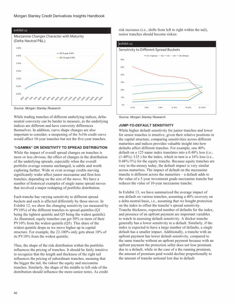
Morgan Stanley Credit Derivatives Insights Handbook
40
exhibit 11
Mezzanine Changes Character with Maturity (Delta-Neutral P&L)
-0.4%
-0.2%
0.0%
0.2%
0.4%
0.6%
0.8%
60%
65%
70%
75%
80%
85%
90%
95%
100%
105%
110%
115%
120%
125%
130%
135%
140%
145%
150%
S9 5-year 6-9%
S9 10-year 6-9%
Source: Morgan Stanley Research
While trading tranches of different underlying indices, delta-neutral convexity can be harder to measure, as the underlying indices are different and have convexity differences themselves. In addition, curve shape changes are also important to consider; a steepening of the 5s10s credit curve would affect 10-year tranches but not the five-year tranches.
“I-GAMMA” OR SENSITIVITY TO SPREAD DISTRIBUTION While the impact of overall spread changes on tranches is more or less obvious, the effect of changes in the distribution of the underlying spreads, especially when the overall portfolio average remains unchanged, is subtle and worth exploring further. Wide or even average credits moving significantly wider affect junior mezzanine and first-loss tranches, depending on the size of the move. We have a number of historical examples of single name spread moves that involved a major reshaping of portfolio distribution.
Each tranche has varying sensitivity to different spread buckets and each is affected differently by these moves. In Exhibit 12, we show the changing sensitivity (as measured by PV10%) of the different tranches to spread quintiles (Q1 being the tightest quintile and Q5 being the widest quintile). As illustrated, equity tranches can get 50% or more of their PV10% from the widest quintile (Q5). This share of the widest quintile drops as we move higher up in capital structure. For example, the 22-100% only gets about 18% of its PV10% from the widest quintile.
Thus, the shape of the risk distribution within the portfolio influences the pricing of tranches. It should be fairly intuitive to recognize that the length and thickness of the right tail influences the pricing of subordinate tranches, meaning that the bigger the tail, the riskier the equity and mezzanine tranches. Similarly, the shape of the middle to left side of the distribution should influence the more-senior notes. As credit
risk increases (i.e., shifts from left to right within the tail), senior tranches should become riskier.
exhibit 12
Sensitivity to Different Spread Buckets
0%
10%
20%
30%
40%
50%
60%
0-3% 3-6% 6-9% 9-12% 12-22% 22-100%
Q1 (Tightest) Q2 Q3 Q4 Q5 (Widest)
Source: Morgan Stanley Research
JUMP-TO-DEFAULT SENSITIVITY While higher default sensitivity for junior tranches and lower for senior tranches is intuitive, given their relative positions in the capital structure, comparing sensitivities across different maturities and indices provides valuable insight into how defaults affect different tranches. For example, one 40% default on a 125 name index translates into a 0.48% loss (i.e., (1-40%) /125 ) for the index, which in turn is a 16% loss (i.e., 0.48%/3%) for the equity tranche. Because equity tranches are very in-the-money today, the default impact is very similar across maturities. The impact of default on the mezzanine tranche is different across the maturities – a default adds to the value of a 5-year investment grade mezzanine tranche but reduces the value of 10-year mezzanine tranche.
In Exhibit 13, we have summarized the average impact of one default on various tranches, assuming a 40% recovery on a delta neutral basis, i.e., assuming that we bought protection on the index to offset the tranche’s spread sensitivity. Tranche thickness, expected number of defaults for the index, and presence of an upfront payment are important variables to watch in assessing default sensitivity. A thicker tranche generally has a lower sensitivity to a default. Similarly, if the index is expected to have a large number of defaults, a single default has a smaller impact. Additionally, a tranche with an upfront payment has lower default sensitivity, compared to the same tranche without an upfront payment because with an upfront payment the protection seller does not lose premium due to a default, while in the case of a the running premium, the amount of premium paid would decline proportionally to the amount of tranche notional lost due to default.

Section A, Chapter 3 Tranche Primer – A Tale of Two Markets
41
exhibit 13
P&L Across the Capital Structure from One Default (Delta-Adjusted)
-10%
-8%
-6%
-4%
-2%
0%
2%
0-3%
3-6%
6-9%
9-12
%
12-2
2%
22-1
00%
0-3%
3-6%
6-9%
9-12
%
12-2
2%
22-1
00%
0-3%
3-6%
6-9%
9-12
%
12-2
2%
22-1
00%
5yr 5yr 5yr 5yr 5yr 5yr 7yr 7yr 7yr 7yr 7yr 7yr 10yr 10yr 10yr 10yr 10yr 10yr
Note: Assuming 40% recovery for IG. Source: Morgan Stanley Research
How do we determine if a tranche has more default risk or spread risk? Delta-neutral default sensitivity, as shown in Exhibit 13, helps us determine the subordination level in the capital structure where tranches transition from being net default sensitive to net spread sensitive. For example, the mezzanine tranche (3-6%) of five-year investment grade is net spread sensitive (i.e., the delta-neutral protection writer will have a positive mark-to-market in case of a default), while the 10-year mezzanine tranche is net default sensitive.
Using the distinction between net default and spread sensitivities of tranches, we can construct trades that are more efficient in expressing our credit views. For example, a combination of long equity and short mezzanine in a delta neutral ratio effectively expresses a credit view that is constructive on default risk but not on spread levels.
“THETA” OR TIME DECAY As a credit default swap approaches maturity, the spread is bound to converge to zero, since credit protection provided by a CDS eventually becomes worthless if a default does not occur. As with any credit/rate product, the passage of time generates return or “time decay”. The “theta” or time decay in tranches is a function of three elements: a) the slope of the credit curve b) reduced time to maturity and therefore reduced riskiness as measured by duration, and c) changes in risk allocation in the index capital structure in different maturities.
exhibit 14
Time Decay for 5yr Tranches Tranche P&L
-6%
-4%
-2%
0%
2%
4%
6%
8%
10%
12%
14%
- 1 2 3 4 5 6 7
Years
0-3%3-6%6-9%9-12%12-22%22-100%
Source: Morgan Stanley Research
The first two factors are fairly simple to understand. In general credit curves are upward sloping, although not always, and even if curves are inverted, the portfolio with the shorter maturity will have a lower duration, which means the index will generate a positive return in a year’s time (assuming no defaults, of course, and that spreads remain unchanged).
exhibit 15
Time Decay as % of Total Return Over 8 Years Share of Total Return in Each Year
0%
5%
10%
15%
20%
25%
1 2 3 4 5 6 7 8
Years
0-3%3-6%6-9%9-12%12-22%22-100%
Source: Morgan Stanley Research
The last factor – risk allocation change due to reduced maturity – is slightly more complicated. Since junior tranches are levered investments on defaults, their value changes faster than the index. Another way to think about this is that as the index gets closer and closer to maturity, the risk tends to flow down the capital structure into the more junior tranches. Exhibit 14 shows the total return of iTraxx S9 five-year tranches for different time horizons, from the perspective of the protection seller. The value of protection declines precipitously initially and decelerates toward the maturity. On an absolute basis, tranches with higher than 1x delta lose value faster than the index, while senior tranches with deltas of less than one lose value more slowly than the index.

Morgan Stanley Credit Derivatives Insights Handbook
42
However, when we analyze a tranche’s time decay relative to itself over time (i.e., how much of the total value is realized every year), we find that equity tranche value decays slower than the index while all other tranches decay faster than the index, in the case of investment grade tranches. For example, equity realizes less than 10% of its cumulative value in each of the early years. Senior tranches such as 12-22% get a higher than average share of the value in early years (see Exhibit 15).
“RHO” OR SENSITIVITY TO CORRELATION As we discussed earlier, junior tranches are long correlation, senior tranches are short correlation and mezzanine tranches are relatively insensitive to correlation. In other words, higher correlation is better for junior tranches and worse for senior tranches (from the perspective of protection sellers). Exhibit 16 shows the sensitivity of 5-year investment grade tranches to parallel shifts in the base correlation curve. For example, for the +5% scenario, we assumed that the equity tranche’s correlation increases 5% and the base correlation skew curve remains unchanged. Thus, for all tranches, the attachment and detachment point correlations change by the same amount. As seen in the Exhibit, the junior tranches generate a positive P&L as correlations rise, whereas super senior tranches are short correlation.
To isolate the impact of correlation changes, we have assumed that the base correlation skew remains unchanged. In practice, skew can and does change. Since base correlation considers all tranches as a portfolio of two equity tranches, as the skew (i.e., the difference between the implied correlations for attachment and detachment points) increases, the par spread decreases, just like the equity tranche. It is important to note that correlation sensitivity of tranches changes as the underlying index spread moves. The more in-the-money the tranche is with respect to index expected losses, the more equity-like the tranche is and therefore the longer the correlation. So as seen in Exhibit 17, the 3-7% tranche will be less sensitive to correlation if spreads tighten a lot as it becomes more at-the-money.
In Exhibit 17, we analyze the mark-to-market impact of a 1% increase in correlation for 5-year investment grade tranches at different spread levels for the index. As shown in the exhibit, senior tranches are relatively correlation insensitive for small changes in spread but become significantly more sensitive as the index widens materially. The converse is true for the equity tranche, i.e., it is rather sensitive for small changes to the index, but beyond a certain point of widening, correlation sensitivity starts to decline.
exhibit 16
Correlation Sensitivity of Tranches (iTraxx S9 7-Year) Tranche P&L
-20%
-15%
-10%
-5%
0%
5%
10%
15%
20%
-20% -15% -10% -5% 0% 5% 10% 15% 20% 25%
Parallel Shift in Correlation Curve
0-3%3-6%6-9%9-12%12-22%22-100%
Source: Morgan Stanley Research
exhibit 17
Correlation Sensitivity vs. Spreads – CDX IG 5-Year
Mark-to-Market Impact of 1% Change in Correlation
-0.2%
0.0%
0.2%
0.4%
0.6%
0.8%
1.0%
0 25 50 75 100 125 150 175 200Index Spread Level (bps)
0-3%3-7%7-10%10-15%15-30%
Source: Morgan Stanley Research
IMPACT OF TRANCHE STRUCTURE ON SENSITIVITY Last but not the least, the pricing structure of the tranche influences the sensitivities meaningfully – a tranche with an upfront payment tends to have a lower delta compared to the same tranche without an upfront payment. Why does an upfront payment lower the delta of a tranche? The answer lies in understanding how rising spreads affect the present value of expected premiums (premium PV) and default PV. An upfront payment with no running coupon implies that as spreads widen, the tranche value is affected only by higher expected defaults, and not lower expected premiums, since the protection seller has already collected the entire premium. On the other hand, an all-running contract will have both negative impacts – higher expected defaults and lower expected premiums due to more defaults making it more sensitive.

Section A, Chapter 3 Tranche Primer – A Tale of Two Markets
43
SECURITIZATION APPROACH: RATIONALE AND UNCERTAINTY In the securitization world, the rationale for using tranches is two-fold. At one level, it allows investors to make portfolio investments in corporate credit with credit enhancement (i.e., protection from some amount of defaults). The rationale here is very similar to what we see in the broader securitization world where the underlying credit risk is a bit more esoteric, including non-agency mortgages, consumer credit like autos and credit cards, and commercial real estate. The second is to be part of the so-called “shadow” banking system itself. Regulators are clearly supportive of the existence of a shadow banking system, where credit is provided through capital market solutions that include securitization.
SECURITIZATION APPROACH: BESPOKE NEW ISSUE Synthetic CDOs, or CSOs, first started appearing in the previous cycle during the rapid growth in popularity and usage of single-name CDS in the default-intensive cycle of 2001-2002. The development of index tranches and correlation technology led to a move away from the fully distributed approach favored by the cash CDO market and more toward the single-tranche CSO model, as dealers were able to more efficiently hedge individual tranche exposure using single-name deltas and correlation hedges in the liquid tranche market. Relative to their cash CDO counterparts in the securitization world, CSOs provided increased flexibility, as synthetic technology made it possible to customize risk exposures with respect to currency, cash flow, tenor, portfolio, maturity, subordination and size of exposure. Since there is no need to identify and acquire a specific asset, the maturity of the transaction is not constrained by the maturity of the pool of assets and furthermore, there is a significantly lower ramp-up period and therefore lower carry costs. Finally, bespoke structures allowed investors to customize an asset according to rating preference and desired yield, something neither the cash CDO market nor the single-name market had been able to do with so much flexibility.
From a mechanics perspective, bespoke mezzanine tranches look less like fully funded cash CDOs and instead better resemble index tranches on the swap side, with a funding component. An SPV is set up, and the investor pays par to the SPV, which in turn purchases eligible collateral to earn a LIBOR based coupon, and then enters into a swap agreement with a dealer (see Exhibit 18). We have covered the various types of collateral in elsewhere (see Chapter 21).
Early transactions had capital structures that were fully placed, usually with a 5-year maturity, mezzanine attachment points ranging from 2% to 10% and thicker tranches on portfolios that were predominantly IG, though it wasn’t until the ratings model changes of late 2005 when HY credits were almost completely eradicated from structures. The bulk of mezzanine issuance that fueled the structured credit machine occurred between 2004 and 2007. The portfolios for these transactions were bespoke in nature, with thin mezzanine tranches and collateral that was either managed by third-party managers,
managed by the investors themselves, or simply static. These transactions were more varied from a performance perspective than their early-cycle counterparts, and we cover the distressed opportunity that arose from these mid-to-later cycle deals later on in this primer.
exhibit 18
Typical Bespoke Mezzanine Funded Structure
Investor pays dollar value for
CLN
Investor receives proceeds from collateral and
unfunded tranche
INVESTOR SPV
EligibleCollateral
SPV buys collateral
Collateral pays coupon
Dealer
SPV sells unfunded
protection on tranche to dealer
SPV receives spread from
dealer
Investor pays dollar value for
CLN
Investor receives proceeds from collateral and
unfunded tranche
INVESTOR SPV
EligibleCollateral
SPV buys collateral
Collateral pays coupon
Dealer
SPV sells unfunded
protection on tranche to dealer
SPV receives spread from
dealer
Source: Morgan Stanley
One question we hear repeatedly is whether structured credit activity will return to the corporate credit market. Whether or not one intends to use synthetic forms of structured credit, flows here had a tremendous impact on investment grade markets in the last cycle, so the question is certainly an important one. From a derivatives perspective, structured credit activity never really died in the cycle as both increased volatility and pronounced amounts of credit risk created unprecedented trading opportunities, mainly in the liquid index tranche markets, and more recently in unfunded bespoke transactions (i.e., in swap form).
From a securitization perspective, however, new issue bespoke volumes came to a standstill, with many investors focused on restructuring their existing, or legacy, bespoke positions to meet ratings and capital guidelines. With the healing of the credit markets, securitization has been deemed vital to the credit system, mainly because it offers lending institutions an efficient alternative to unsecured borrowings (hence the motivation for the government programs). The source of this efficiency comes from the secured nature of the borrowing, the economies of scale associated with pooling assets into portfolios, and the cheaper costs of taking first loss exposure and borrowing against tail risks. Given that securitization is most prevalent in cash securities, issuers (mainly banks) benefit most directly.
SECURITIZATION APPROACH: DISTRESSED MEZZANINE In early 2009 we first identified the enormous opportunity that the legacy bespoke mezzanine market was offering in the wake of the downgrade and default of many corporate issuers (see Chapter 20), causing traditional bespoke mezzanine investors to liquidate their holdings for a variety of reasons, including ratings downgrades, changes in internal investing rules from risk managers, and others who were spooked by the markets in

Morgan Stanley Credit Derivatives Insights Handbook
44
general and were fleeing to higher quality assets. Most of these assets were bespoke transactions from the 2004-2007 vintages and were trading at highly distressed levels. For anyone willing to put into place the necessary tools to evaluate these structures, there were plenty of opportunities to be had. We categorized the distressed assets as follows:
IO-Value. These are the low dollar price instruments (below $10), which are priced like IOs – typically equal to about 2-3 years of coupon. It is expected that the principal value will be little to nothing at maturity; the valuation is based on the expectations for how many coupons the structure will pay out before the notional goes to zero. The yield to maturity of these structures could be in the 60%+ range.
Option-Value. These are mid-priced structures ($5–30) that capture the interest component plus the small potential likelihood of principal recovery as well. Yields for these deals are likely in the 30-60% range.
Potentially Money-Good. These structures can have any or all of the following: shorter maturities, cleaner portfolios, higher subordination, greater thickness – and consequently they have higher prices associated with them ($20–80). These are categorized as potentially money-good because while nowhere near a certainty, the likelihood that there will be at least a partial principal repayment is higher. Yields here are much lower (25–50%) but still fairly attractive compared to the high single-digit and low-to-mid-teen risk-adjusted returns for plain vanilla IG/loans or HY credit.
The primary driver of value in the legacy mezzanine bespoke market was tail risk. Exhibit 19 illustrates just how much wider the tail names that were common constituents in many CSOs were than the CDX IG index at the peak of 2008. The distressed mezzanine opportunity is and was primarily a levered play on spread compression and healing in this part of the portfolio.
exhibit 19
Top 100 CSO Names vs. CDX
0
100
200
300
400
500
600
Mar-06 Sep-06 Apr-07 Nov-07 May-08 Dec-081.0
1.2
1.4
1.6
1.8
2.0
2.2
2.4
2.6
Top 100 CDO Credits IndexCDX IG ROTRRatio of CDO basket spread/CDX
Source: Morgan Stanley Research
Taking advantage of this dislocation required some background knowledge of the market, though we highlighted when we first identified this opportunity that correlation models aren’t as necessary here as they were earlier. Instead, we argued that investors should focus on the following characteristics to determine value:
Subordination. Many of the financials defaults were common names in bespoke CLNs and thus many of these assets had at least some loss of subordination.
Thickness. Thin tranches were the dominant theme when these assets were originally structured, to increase structural leverage and thus spread. This matters because if the tranche were touched at all, it could potentially require only one additional default for full write-down. This is very different from the index tranches, which are all at least 3% thick and can withstand a greater number of defaults once breached.
Portfolio composition. This is clearly important, particularly if there is little subordination left in the structure. Tail risk in particular is a primary concern. To combat some of the extreme dispersion present in these portfolios, we indicated a preference for paying for risk management and recommended using some amount of the coupon income to pay for a manager and/or buying protection on tail names.
Recovery. The majority of these structures are floating recovery, and recovery can be much lower than expected at times. Some, however, are fixed recovery, generally 40%, and this added certainty regarding number of defaults needed to impact the tranche can be very valuable.
Managed or static. Some CLNs are managed synthetics, and the added presence of a manager can be valuable, depending on the manager.
Maturity. Earlier vintage deals had much shorter maturities while transactions done in the 2006-2007 time period were typically 7-10yrs. We argue that maturity is far less important than the first five components listed above, though still worth noting, particularly in the very short end.
Coupon. While we argue that the deeply discounted dollar price is the more eye-catching price component, for those bespokes we consider to fall under the category of “IO opportunity”, coupon is important.
SECURITIZATION APPROACH: RATINGS METHODOLOGY Rating agencies have been an important part of the tranche market since inception. Because ratings are closely linked to the capital held against CSO tranches, we expect the agencies to wield considerable influence on the trajectory of the CSO market in the future, especially in the post-Basel II environment. While the synthetic CSO market has evolved considerably since its introduction ten years ago, the core of

Section A, Chapter 3 Tranche Primer – A Tale of Two Markets
45
the rating agency approach has remained relatively constant. (See “CDO Evaluator Applies Correlation and Monte Carlo Simulation to Determine Portfolio Quality” by S&P, November 13, 2001; “Moody’s Approach to Rating Corporate Collateralized Synthetic Obligations” by Moody’s, September 14, 2009; and “Update to Global Methodologies and Assumptions for Corporate Cash Flow and Synthetic CDOs” by S&P, September 17, 2009). Both S&P and Moody’s use a Gaussian copula model as the basis for inferring portfolio default distributions from a set of individual default assumptions and correlations amongst various assets in the portfolio. Both S&P and Moody’s methodologies specify for each credit a) some kind of default rate trajectory based on ratings of the underlying portfolio names and b) recovery assumptions based on the domicile, sector and nature of the credit in the portfolio.
Although the methodology remains same, the threshold levels for the default rates, recoveries and asset correlations have undergone various changes over time. One of the important shifts was the change in default rate inputs by S&P in 2005, which benefitted IG corporates and penalized HY corporates. A positive outcome of this was that much of the CSO portfolios from 2006 did not have much high yield exposure, though they had heavy concentrations of financials and insurers instead. The heavy presence of banks (including the Icelandic banks, Washington Mutual, Lehman) and the insurers proved to be the weakest link for CSOs in the 2008-09 default cycle and distressed financials continue to dominate the tails of legacy CSOs.
exhibit 20
Ratings Distribution of Sample CSO Tranches
3% 5%
36%43% 46% 49% 52% 57% 58% 60% 61%
81% 81% 80% 80%
10%15%
18%
18% 16%15%
14%12% 12% 13% 13%
7% 7% 7% 7%
12%
14%
8%7% 7% 6% 6% 6% 7% 6% 6%
6% 6% 6% 6%
32%30%
15%13% 13% 12% 11% 10% 9% 9% 8%
3% 3% 4% 4%
43%37%
23% 19% 18% 18% 17% 15% 15% 13% 13%3% 3% 3% 3%
0%
10%
20%
30%
40%
50%
60%
70%
80%
90%
100%
Nov-07
Aug-08
Nov-08
Dec-08
Jan-0
9
Feb-09
Mar-09
Apr-09
May-09
Jun-0
9Ju
l-09
Nov-09
Jan-1
0
Apr-10
May-10
AAAAAABBBSub-IG
Source: S&P, Morgan Stanley Research
Post-crisis, the rating agencies have once again altered the CSO landscape by making ratings criteria more stringent. The experience with sub-prime CDOs caused rating agencies to scale up default assumptions and correlations while also
lowering assumed recoveries and introducing additional stress tests and safeguards. These include, among others, applying additional stresses to base default rates and introducing concentration tests for sector and geographic location and are particularly stringent for tranches that will be rated AAA. All these changes have made achieving AAA/AA ratings with a viable yield difficult to achieve for any new potential CSOs.
The changes to methodologies have also contributed to turning the ratings distributions of legacy CSOs upside down – from just 3% of the universe below investment grade in 2007, to more than 80% today. As seen in Exhibit 20, the CSO universe suffered two shocks – one in late 2008 due to the default of the financials and the second in the second half of 2009 due to the ratings criteria change.
As we mentioned earlier, both S&P and Moody’s have broadly similar approaches in terms of arriving at portfolio default rates. The key difference between the two agencies is that while S&P focuses on the probability of default of the tranche, Moody’s focuses on the expected losses from the tranche. The result is that Moody’s assigns different ratings to tranches of same attachment but different thicknesses, whereas S&P would give the same rating for tranches of same attachment point, regardless of tranche thickness. Both agencies emphasize additional overrides to the model suggested ratings in changes to methodologies made after the crisis.
Both agencies have a similar approach to specifying correlations. Moody’s correlation assumptions are based on a) the inter-industry correlation, which applies to two corporates in different sectors, and b) the intra-industry correlation, which applies to two corporates within a same sector. Moody’s also classifies industries as “global”, “semi-local”, or “local” to describe the extent to which credits within a single industry, but in different regions, are correlated. In a similar vein, S&P specifies correlation parameters for a) firms in the same corporate industry and b) firms in different corporate industries. In addition, S&P assigns a correlation factor between assets from different industries in different geographic regions.
With respect to recovery assumptions, both agencies now use recovery assumptions that are correlated to the default levels in the simulations. Both agencies link the mean and volatility of the recovery for each credit in the portfolio based on the type of credit (bond vs. loan) or priority/seniority (secured or unsecured) and jurisdiction of the entity.
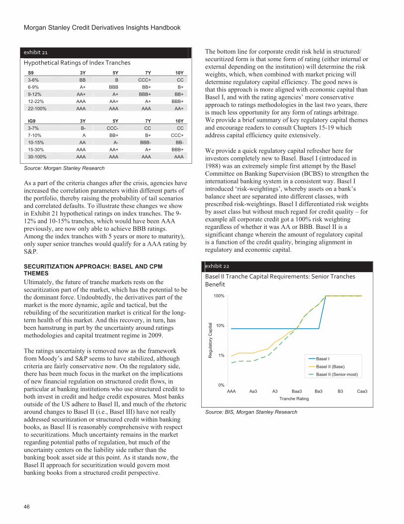
Morgan Stanley Credit Derivatives Insights Handbook
46
exhibit 21
Hypothetical Ratings of Index Tranches S9 3Y 5Y 7Y 10Y 3-6% BB B CCC+ CC 6-9% A+ BBB BB+ B+ 9-12% AA+ A+ BBB+ BB+ 12-22% AAA AA+ A+ BBB+ 22-100% AAA AAA AAA AA+ IG9 3Y 5Y 7Y 10Y 3-7% B- CCC- CC CC 7-10% A BB+ B+ CCC+ 10-15% AA A- BBB- BB- 15-30% AAA AA+ A+ BBB+ 30-100% AAA AAA AAA AAA
Source: Morgan Stanley Research
As a part of the criteria changes after the crisis, agencies have increased the correlation parameters within different parts of the portfolio, thereby raising the probability of tail scenarios and correlated defaults. To illustrate these changes we show in Exhibit 21 hypothetical ratings on index tranches. The 9-12% and 10-15% tranches, which would have been AAA previously, are now only able to achieve BBB ratings. Among the index tranches with 5 years or more to maturity), only super senior tranches would qualify for a AAA rating by S&P.
SECURITIZATION APPROACH: BASEL AND CPM THEMES Ultimately, the future of tranche markets rests on the securitization part of the market, which has the potential to be the dominant force. Undoubtedly, the derivatives part of the market is the more dynamic, agile and tactical, but the rebuilding of the securitization market is critical for the long-term health of this market. And this recovery, in turn, has been hamstrung in part by the uncertainty around ratings methodologies and capital treatment regime in 2009.
The ratings uncertainty is removed now as the framework from Moody’s and S&P seems to have stabilized, although criteria are fairly conservative now. On the regulatory side, there has been much focus in the market on the implications of new financial regulation on structured credit flows, in particular at banking institutions who use structured credit to both invest in credit and hedge credit exposures. Most banks outside of the US adhere to Basel II, and much of the rhetoric around changes to Basel II (i.e., Basel III) have not really addressed securitization or structured credit within banking books, as Basel II is reasonably comprehensive with respect to securitizations. Much uncertainty remains in the market regarding potential paths of regulation, but much of the uncertainty centers on the liability side rather than the banking book asset side at this point. As it stands now, the Basel II approach for securitization would govern most banking books from a structured credit perspective.
The bottom line for corporate credit risk held in structured/ securitized form is that some form of rating (either internal or external depending on the institution) will determine the risk weights, which, when combined with market pricing will determine regulatory capital efficiency. The good news is that this approach is more aligned with economic capital than Basel I, and with the rating agencies’ more conservative approach to ratings methodologies in the last two years, there is much less opportunity for any form of ratings arbitrage. We provide a brief summary of key regulatory capital themes and encourage readers to consult Chapters 15-19 which address capital efficiency quite extensively.
We provide a quick regulatory capital refresher here for investors completely new to Basel. Basel I (introduced in 1988) was an extremely simple first attempt by the Basel Committee on Banking Supervision (BCBS) to strengthen the international banking system in a consistent way. Basel I introduced ‘risk-weightings’, whereby assets on a bank’s balance sheet are separated into different classes, with prescribed risk-weightings. Basel I differentiated risk weights by asset class but without much regard for credit quality – for example all corporate credit got a 100% risk weighting regardless of whether it was AA or BBB. Basel II is a significant change wherein the amount of regulatory capital is a function of the credit quality, bringing alignment in regulatory and economic capital.
exhibit 22
Basel II Tranche Capital Requirements: Senior Tranches Benefit
0%
1%
10%
100%
AAA Aa3 A3 Baa3 Ba3 B3 Caa3
Tranche Rating
Reg
ulat
ory
Cap
ital
Basel I
Basel II (Base)
Basel II (Senior-most)
Source: BIS, Morgan Stanley Research

Section A, Chapter 3 Tranche Primer – A Tale of Two Markets
47
While Basel II is new to the US, European banks have already adhered to Basel II since 2008. As is clear from the discussion above, banks with a greater proportion of IG assets may actually end up reducing their risk-weighted assets. In a world where banks err towards more liquid and higher quality credit and have greater amount of buffers, Basel II could end up being more favorable from an asset perspective. If the European Banks’ experience is any indicator, most large banks will ultimately seek approval from regulators to use the Advanced Internal Ratings Based Approach (AIRB). AIRB specifies methods to calculate the risk weighting based on internal estimates of the Probability of Default (PD), Exposure at Default (EAD) and Loss Given Default (LGD).
Because Basel II regulatory capital is closely aligned with economic capital, changes in market pricing can influence strategies to a greater extent than did Basel I. While senior tranches generally benefit relative to junior tranches, relative value perceptions – for example, between junior mezzanine and senior mezzanine or between senior and super senior – can change based on the pricing.
exhibit 23
Basel II Corporate Risk Capital Requirements: High Quality Credit Benefits
0%
2%
4%
6%
8%
10%
12%
14%
16%
AAA Aa3 A3 Baa3 Ba3 B3Rating
Reg
ulat
ory
Cap
ital
Basel IFoundation IRBAdvanced IRB
Note: IRB – Internal Ratings Based Approach. Source: BIS, Morgan Stanley Research
Impact on CSO market. As far as bespoke CSOs from the last cycle are concerned, they are deeply underwater from a ratings perspective, as we have highlighted previously. Clearly, these mostly mezzanine CSOs look unfavorable under Basel II. Despite the ratings issue that has existed for some time now, unappetizingly low valuations were a key impediment for sellers early in 2009, as were lacks of both an organized buyer base and adequate depth. However, a maturing ratings-insensitive buyer base has developed in 2010 and has largely been able to absorb these sales as they occur. Orderly CSO BWICs were a regular occurrence in 1H 2010 and appetite for secondary CSO paper remained fairly strong.
Securitization and Capital Relief Strategies. Last but not least, securitization and capital relief strategies have experienced a complete U-turn from Basel I to Basel II. The most common Basel I strategy involved retaining the yieldiest part of the capital structure, i.e., the equity tranche, and buying protection on 3-100% part of the capital structure. Under Basel II, the optimal strategies for Europe proved to be the exact opposite – the focus is on what part of the capital structure is most efficient to retain, and as we discussed above, it is now the senior, higher quality tranches that are the most attractive risk to retain. Investors have a number of types of hedging choices (see Exhibit 24).
exhibit 24
Thinking About Structured Hedging Alternatives
Long Index
5-100% tranche risk retained
Equity tranche (0-5%) hedged
9-100% tranche risk hedged
Equity tranche (0-5%) hedged
5-9% retained
9-12% hedged
Equity tranche (0-5%) hedged
12-100% tranche risk retained
5-9% retained
2T – H-L
3T – H-L-H
4T – H-L-H-L
Sell Protection on 5-100% tranche risk
Equity tranche (0-5%) No position
2T – N-L
Source: Morgan Stanley Research

Morgan Stanley Credit Derivatives Insights Handbook
48
Chapter 4
Baskets Go Back to the Future February 26, 2010
Sivan Mahadevan Ashley Musfeldt Phanikiran Naraparaju
First-to-default, or more generally, nth-to-default, baskets were one of the credit derivatives market’s earliest instruments, dating back to the beginnings of the CDS contract itself in the late 1990s. Such baskets (which typically have exposures to less than 10 corporate or sovereign credits) have much in common with the broader world of tranches on larger portfolios in that they have “correlation” risk. However, the smaller basket market tends to fall in the middle of the large worlds of single-name CDS and portfolio tranches, and it has even been ignored by market participants for extended periods as investors instead focused on the larger flows in CDS and portfolio tranches.
exhibit 1
Basket Pricing Depends on Correlation
050
100150
200250300
350400
450500
10% 20% 30% 40% 50% 60% 70% 80% 90%
FTD2TD2-LTD
Source: Morgan Stanley Research
As structured credit heals from the fall-out of the credit crisis, there is certainly a “back to simplicity” bid in the market, and as such, we see increased flows in simple baskets from investors, both as buyers and sellers of protection. The motivation includes still wide credit spreads in many corporate sectors, reasonably high correlation, and stress in the sovereign and US municipal sectors, both of which have burgeoning single-name CDS markets. Given our fair value to constructive views on corporate credit along with our belief that default correlation has room to continue to fall, we in general like buying FTD protection and selling 2nd-to-Nth to default protection in today’s market environment, but details certainly matter. In the remainder of this chapter, we provide some recent history and updates on the FTD/NTD basket market, some examples of investment and hedging strategies that we favor today, and an updated primer on the market.
NOTIONAL BASKET HISTORY FTDs began trading, as we mentioned earlier, very early on in the CDS market. Initially they were simple tools to get additional structural leverage on a basket of names. While they were and are a correlation product, they behave differently from tranches in that when a name in the basket is triggered, they behave more like single-name CDS contracts than tranches because the “loss” doesn’t erode subordination, but rather the entire name is removed and settled separately like a single-name contract. In the case of FTDs, after this one default, the contract is over then, regardless of recovery. This structural simplicity makes them easier to deal with than tranches, and this is why many investors then found them to be a good introduction to the correlation market. As the CDS and structured credit market matured in 2003-2006, FTDs fell in popularity as bespoke tranches on much larger “baskets” (more appropriately deemed portfolios) of 100+ names became the bread-and-butter product of most structured credit market participants.
exhibit 2
Investor Motivation for Basket Trading
Basket Protection Seller Protection Buyer
FTD � Receive higher yield for same notional by taking more levered exposure to basket
� Express credit views in levered form
� Position for rising correlation
� Avoid idiosyncratic risk on a basket
� Buy cheaper protection vs. individual swaps on all underlying names, but retain tail risk
� Express views of falling correlation between individual names or industries
2nd-through-Nth
� Express positive views on a basket, while avoiding idiosyncratic risk, but taking tail risk
� Receive possibly higher yield than some of the low yielding names in the underlying basket
� Position for falling correlation
� Buy cheaper protection against the tail risk vs. buying protection on all underlying names
� Manage risk for extreme scenarios
Source: Morgan Stanley, Moody’s
In late 2006 we saw a brief resurgence of interest in FTDs, though bespoke tranches still ruled the day, but this time we saw greater two-way flows and more interest in other default baskets, such as second-to-defaults (2TDs), second-through-last-to-defaults (2-LTDs), higher Nth-to defaults (NTDs) and even some Nth-through-last-to-defaults (N-LTDs). Investors this time around were interested in using these products for sector plays, to get either long or short 5-10 names in a sector, as de-levered hedges with low carry,

Section A, Chapter 4 Baskets Go Back to the Future
49
such as 2-LTDs, or as a levered way to play a small basket of high conviction longs.
Now, after another dry spell brought on understandably by the credit crisis, we are again seeing a resurgent interest in these products. Again we are seeing interest in both FTDs and their unlevered senior cousins 2-LTDs. We are seeing interest in these in both swap and CLN form based on investor type. Some new additions this time around, however, are the constituent base; namely European sovereign and US muni CDS are now being put into baskets
STRUCTURAL OVERVIEW An Nth-to-default basket is a product in which the investor gains either long or short exposure to a relatively small basket of credits. The typical size of baskets ranges from 4 to 10 credits. The investor is either selling or buying protection on the Nth credit to default in the basket, as with a plain vanilla credit default swap, except that the reference credit is a basket instead of a single name. Five-name baskets are most common, and protection is typically bought or sold on either First-to-Default (FTD) or 2nd-through-last-to-default (2-LTD).
Suppose an investor sells FTD protection on a five-name basket of reference credits. The investor will receive a periodic payment (the “premium”) in exchange for taking on the credit risk of the basket. If no credit events occur during the term of the basket default swap, the swap expires. If a credit event occurs during the term of the basket, the swap is terminated and the seller of protection in the basket loses par minus the recovery value of the defaulted asset, and the single-name contract is settled via the ISDA auction process. This process is analogous to a single-name credit default swap. Exhibit A1 shows an FTD swap with an underlying basket of five names:
exhibit A1
Nth-to-Default Structure
Source: Morgan Stanley Research
We also note that FTD and NTD baskets have “cousins” in other markets, most notably equities and currencies, where option flows in “best of” and “worst of” baskets are quite common. Taking equities as an example, it is common for investors to, for example, buy a call option on the “worst performing” name in a small basket of stocks, as a way of cheapening the premium vs. the alternatives (buying call options on each of the individual stocks, or buying a call option on the whole basket). Such a strategy is long correlation.
exhibit A2
FTDs’ Cousins in the Equity Markets
Credit Strategy
Equity Strategy
Correlation Exposure
Rationale
Buy FTD Protection
Buy Worst of Put
Short Correlation
Buy put or default protection on “worst” name, so you have first-loss hedging without buying puts or protection on full portfolio (smaller notional exposure)
Sell FTD Protection
Sell Worst of Put
Long Correlation
Take a bullish view on defaults or equity price performance and position for the scenario that all assets do well or avoid default.
Source: Morgan Stanley
In comparing these equity strategies to FTD baskets, it is probably best to focus on puts. In Exhibit A2 we highlight common strategies. Buying a worst of put in equities would be similar to buying first-to-default protection, in that one has “protection” from the worst name (but not the others), and it is a short correlation strategy.
FTD MECHANICS AND CORRELATION Although basket default swaps resemble single-name credit default swaps mechanically, particularly in the event of default, their risk/return and valuation profiles are more akin to bespoke tranches. FTD baskets are thus analogous to equity tranches, 2TDs would be mezz-like, and 2-LTDs are similar to senior or super senior tranches. Even if fully funded, the default swap basket can be thought of as a levered investment on a basket of credits, with non-recourse leverage provided by the counterparty. The seller of protection in an FTD, however, is only exposed to the first credit event, and the principal loss is directly related to the recovery value of the defaulted asset. This aspect is unlike equity tranches, where the trade can still remain after the first loss and will remain until it matures or experiences enough losses to wipe out the tranche.
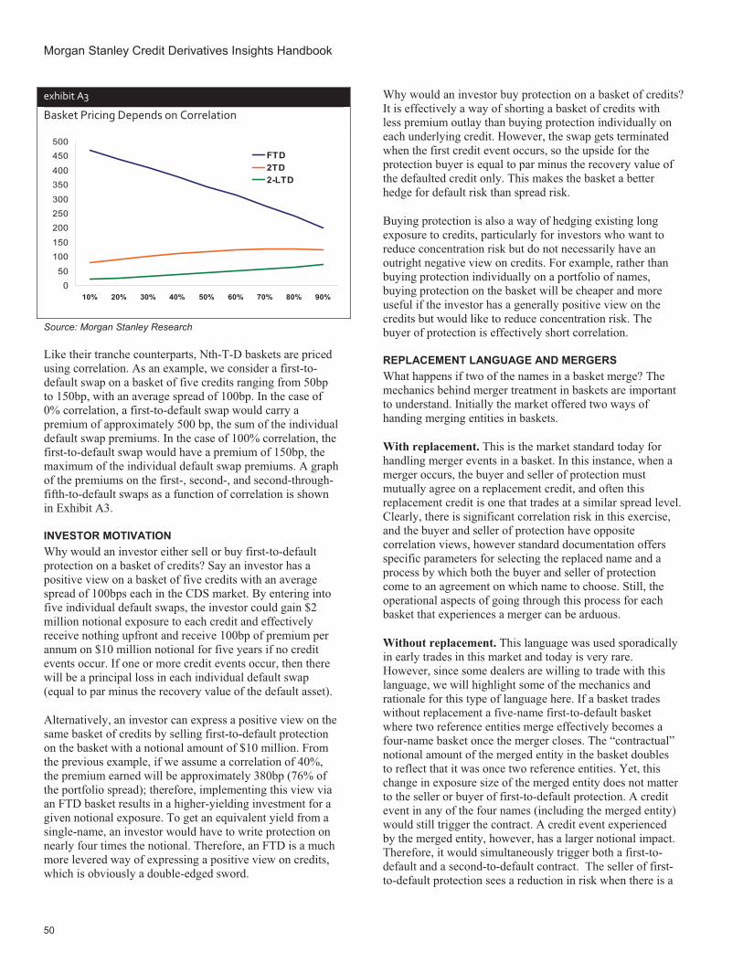
Morgan Stanley Credit Derivatives Insights Handbook
50
exhibit A3
Basket Pricing Depends on Correlation
050
100150
200250300
350400
450500
10% 20% 30% 40% 50% 60% 70% 80% 90%
FTD2TD2-LTD
Source: Morgan Stanley Research
Like their tranche counterparts, Nth-T-D baskets are priced using correlation. As an example, we consider a first-to-default swap on a basket of five credits ranging from 50bp to 150bp, with an average spread of 100bp. In the case of 0% correlation, a first-to-default swap would carry a premium of approximately 500 bp, the sum of the individual default swap premiums. In the case of 100% correlation, the first-to-default swap would have a premium of 150bp, the maximum of the individual default swap premiums. A graph of the premiums on the first-, second-, and second-through-fifth-to-default swaps as a function of correlation is shown in Exhibit A3.
INVESTOR MOTIVATION Why would an investor either sell or buy first-to-default protection on a basket of credits? Say an investor has a positive view on a basket of five credits with an average spread of 100bps each in the CDS market. By entering into five individual default swaps, the investor could gain $2 million notional exposure to each credit and effectively receive nothing upfront and receive 100bp of premium per annum on $10 million notional for five years if no credit events occur. If one or more credit events occur, then there will be a principal loss in each individual default swap (equal to par minus the recovery value of the default asset).
Alternatively, an investor can express a positive view on the same basket of credits by selling first-to-default protection on the basket with a notional amount of $10 million. From the previous example, if we assume a correlation of 40%, the premium earned will be approximately 380bp (76% of the portfolio spread); therefore, implementing this view via an FTD basket results in a higher-yielding investment for a given notional exposure. To get an equivalent yield from a single-name, an investor would have to write protection on nearly four times the notional. Therefore, an FTD is a much more levered way of expressing a positive view on credits, which is obviously a double-edged sword.
Why would an investor buy protection on a basket of credits? It is effectively a way of shorting a basket of credits with less premium outlay than buying protection individually on each underlying credit. However, the swap gets terminated when the first credit event occurs, so the upside for the protection buyer is equal to par minus the recovery value of the defaulted credit only. This makes the basket a better hedge for default risk than spread risk.
Buying protection is also a way of hedging existing long exposure to credits, particularly for investors who want to reduce concentration risk but do not necessarily have an outright negative view on credits. For example, rather than buying protection individually on a portfolio of names, buying protection on the basket will be cheaper and more useful if the investor has a generally positive view on the credits but would like to reduce concentration risk. The buyer of protection is effectively short correlation.
REPLACEMENT LANGUAGE AND MERGERS What happens if two of the names in a basket merge? The mechanics behind merger treatment in baskets are important to understand. Initially the market offered two ways of handing merging entities in baskets.
With replacement. This is the market standard today for handling merger events in a basket. In this instance, when a merger occurs, the buyer and seller of protection must mutually agree on a replacement credit, and often this replacement credit is one that trades at a similar spread level. Clearly, there is significant correlation risk in this exercise, and the buyer and seller of protection have opposite correlation views, however standard documentation offers specific parameters for selecting the replaced name and a process by which both the buyer and seller of protection come to an agreement on which name to choose. Still, the operational aspects of going through this process for each basket that experiences a merger can be arduous.
Without replacement. This language was used sporadically in early trades in this market and today is very rare. However, since some dealers are willing to trade with this language, we will highlight some of the mechanics and rationale for this type of language here. If a basket trades without replacement a five-name first-to-default basket where two reference entities merge effectively becomes a four-name basket once the merger closes. The “contractual” notional amount of the merged entity in the basket doubles to reflect that it was once two reference entities. Yet, this change in exposure size of the merged entity does not matter to the seller or buyer of first-to-default protection. A credit event in any of the four names (including the merged entity) would still trigger the contract. A credit event experienced by the merged entity, however, has a larger notional impact. Therefore, it would simultaneously trigger both a first-to-default and a second-to-default contract. The seller of first-to-default protection sees a reduction in risk when there is a

Section A, Chapter 4 Baskets Go Back to the Future
51
merger, so the seller of second-to-default protection must see an increase in risk, for which he or she must be compensated. We would argue that the merger option is one factor that keeps implied correlation in small baskets higher than in large baskets.
exhibit A4
Replacement Mechanics
Source: Morgan Stanley Research
SECOND-THROUGH-NTH-TO-DEFAULTS A second-through-Nth default basket is similar to a senior tranche, and any credit events after the first default trigger the contract. Unlike FTD baskets, the swap remains in effect until maturity or until all the covered credits default. The risk/return profile is similar to that of a senior tranche in that a protection seller is protected from idiosyncratic risk, but exposed to severe loss scenarios where multiple credits default (also known as “tail risk”). However, a key
difference is that the return profile of the protection seller in a second-through-fifth default basket is independent of the severity of the first loss.
Why would an investor sell protection on a second-through-fifth default basis? As with senior versus equity tranches, selling protection in a second-through-fifth default basket is potentially a safer or less volatile way to gain long exposure to a basket of credits. In exchange for a smaller premium, the protection seller has direct exposure to any defaults after the first credit event, but is protected from the first credit event. An investor with a positive view on the underlying credits can sell protection in this swap and potentially earn more premium than selling protection on some of the individual names. In contrast to first-to-default baskets, the seller of protection is short correlation (i.e., an increase in correlation among the underlying names would have a negative impact).
Why would an investor buy protection on a second-through-fifth default basket? In general, it can be a significantly cheaper way of hedging existing long credit exposure when the investor is willing to take the risk of some losses on the first credit event, but wants to hedge against more severe default scenarios.
FUNDED BASKETS Most basket default swaps are structured and executed in “unfunded” form and are not assigned credit ratings. However, it is possible to combine an FTD basket with a deposit to create a funded product. In that case, the protection writer would buy a note with spread over Libor coming from an FTD position. In case of a default in the underlying portfolio, the note holder would incur a loss of principal on the note, reflecting the payment of par minus recovery on the FTD basket.

Morgan Stanley Credit Derivatives Insights Handbook
52
Chapter 5
Basis Basics in a Normalized World March 19, 2010
Sivan Mahadevan Ashley Musfeldt Phanikiran Naraparaju
From the beginnings of the corporate CDS markets, one of the most basic valuation measures has involved comparing a corporate bond with a CDS contract. While it is simple in concept, this basis relationship is quite complicated, as one instrument is not necessarily an easy substitute for the other. That complexity led many to treat basis trades as an investment strategy with an opportunity to arbitrage pricing and earn carry for taking on specific “basis” risks. Consequently, large basis books were built up across the financial markets.
However, the basis opportunity was perhaps oversimplified, and many basis trades suffered from the actual differences between the instruments during the financial crisis. Differences range from “bond math” type things like coupons, duration, price, yield, and convexity to much broader market themes like liquidity, deliverability/fungibility and of course funding costs. In fact the last point is one that is lost on most pricing models as the dearness of capital at the peak of the crisis pushed the basis to levels that were more negative (cash trading wider than CDS) than the market had ever seen in the history of the CDS market.
The negative basis trade post-Lehman was a significant market opportunity (along with many others), and one that we argued required a long holding period to realize value (see The Basis Moves from a Trade to an Asset, October 31, 2008). Today, the corporate basis relationship has nearly completely healed from the systemic woes that began with the Lehman bankruptcy, as liquidity has returned to the market. While the basis remains negative in the US, it is and has actually been positive in Europe for some time.
So in a more normalized world of funding, liquidity, and risk premiums, we see a return to more normalized basis relationships, and market themes can push the basis to one extreme or the other. Trading the basis is a notion that feels like it is back in markets today; however, as we highlighted above, basis trades do have a funding/liquidity component to them that we are not willing to ignore even if it remains difficult to model. In a sense, the market should demand a premium for taking on this risk, and can look to funding markets as a guide. In this chapter, we use our pre-crisis, crisis, and post-crisis experience with the corporate basis relationship to provide our thoughts on basis relationships generally. Summaries of the themes are below.
Over a decade of history. From the early days of CDS, the corporate basis relationship has moved through several cycles.
It started out as positive owing to the “youth” of the then CDS contract and high default risk in the 2001/2002 credit cycle. The basis then moved to being consistently negative in the midst of the demand for synthetic credit during the structured credit bid during 2004-2007. Extreme negative basis levels appeared during the peak of financial crisis as funding became dear, but today we have moved to a more normalized environment.
Basis metrics: Over the years, we have developed three approaches to measuring the relative value of CDS vs. corporate bonds. We review our simple raw basis measure, more elaborate adjusted basis measure, and our fair value CAPS basis model to gain some insight into valuation.
Interest rate impact. Rates too can have an impact on basis pricing, as rates impact both bond pricing and discounts on CDS upfronts, as well as play a role in determining the steepness of CDS curves. We examine the impact of potentially rising rates on the basis.
High yield as a special case. The high yield basis has always been a different animal than the investment grade one, owing to a variety of factors including higher default probabilities, dollar price differences, the structure of cash flows and of course the callable nature of much of the market (a meaningful portion of the HY universe is callable). The high yield basis still trades at more negative levels than investment grade in both the US and Europe.
A BIT OF HISTORY OF CORPORATE CDS FLOWS Corporate CDS markets were established in the mid-1990s, mainly as a way for banks to hedge their loan exposures, and much of the initial shape of the contract (restructuring risk, shorter maturities) was influenced by this community. But a one-way trade never makes markets, so it was critically important for the market to embrace CDS from an investment perspective as well. As such, in the late 1990s and early 2000s, CDS took a form that was more “bond-like” and subsequently the contract became more investor friendly.
As the CDS market development progressed, we began to see large investment flows through the sale of protection in corporate CDS contracts, mainly in portfolio form through structured credit and market indices. This natural seller of protection was an important factor in market growth by providing a balance in the market. Eventually this flow became a dominant force for CDS market performance, at least until the systemic risk period of the recent crisis, although even during the crisis cash products suffered more from their inherent funding disadvantage. The most recent changes to the corporate CDS market – the big and small bang protocols – have made the contract more fungible by

Section A, Chapter 5 Basis Basics in a Normalized World
53
standardizing coupons, requiring adherence with ISDA protocols, and addressing the concerns surrounding restructuring risk.
exhibit 1
Evolution of Corporate CDS-Cash Basis (2004-07)
CDS - Cash Basis (bp)
-50
-40
-30
-20
-10
0
10
20
30
Sep-04 Mar-05 Sep-05 Mar-06 Sep-06 Mar-07 Sep-07
A positive basis encourages development of a long investor base in CDS.
Funding advantages of CDS and structured credit activity helps CDS outperform and pushes the basis into negative Credit crisis and funding
squeeze hurts bonds relative to the CDS pushing basis to extreme negative levels
CDS underperforms on super-senior concerns but cash remains supported
Source: Morgan Stanley Research
Throughout the history of the development of the CDS market, the basis between CDS and cash bonds has been an important relationship to monitor. Cash bonds once helped price CDS contracts, as cash bond spreads over Libor were the starting point to evaluate credit risk in CDS, after which they were adjusted for restructuring credit events and cheapest-to-deliver optionality. In the early days, CDS generally traded wide to cash instruments as the newness and nuances of the contract motivated protection sellers to demand a premium. Indeed the positive basis was a marketing point for market-makers wishing to promote liquidity in the derivatives contracts. As CDS markets matured, differences became more granular, and market participants built more sophisticated models. In these early days funding costs of cash instruments were largely ignored and liquidity on both sides of the basis remained robust.
exhibit 2
Evolution of Corporate CDS-Cash Basis (2007-10)
Source: Morgan Stanley Research
The corporate negative basis trade – positive carry long bond vs. buy protection through CDS – that emerged circa 2004 was essentially a balance sheet usage allowance for those investors who were able to fund at attractive levels and use this balance sheet to earn a small carry for taking on some amount of counterparty risk, but no actual credit default risk. Regulatory capital charges (for banks) for perfectly matched bond and CDS positions were and continue to be minimal for basis trades. There was also the added benefit of optionality through covenanted basis packages. Investors bought bonds with covenants (poison puts, rating step-ups) which outperform in LBO/M&A scenarios and with ratings deterioration, and buy CDS protection. The basis trade played a part in absorbing protection sold by investors in structured credit and at the same time provided the investment community with a way to retain illiquid secondary market cash positions.
Around 2005 the cash-CDS basis turned negative, and has remained largely negative ever since, save for a short period when super senior concerns drove it into positive territory (see Exhibit 2). From 2005 to 2007, the basis traded primarily in the negative 15 to 20bp range. In an environment where AAA/AA assets traded under 10bp, 15-20bp seemed reasonable compensation for basis trades at that time.
In 2008 the basis started dipping to new lows in the negative 50bps range and hovered there until the Lehman bankruptcy triggered a larger credit squeeze. Conventional wisdom would suggest that CDS should underperform cash bonds in a high default environment, given the fact that CDS is a pure play on credit risk, whereas cash bonds are a combination of interest rate and credit risk and are short cheapest-to-deliver optionality. However, during the credit crisis, liquidity issues trumped default spreads, with balance sheet usage becoming a bigger concern for investors and the market than default risk. The basis re-priced to unseen levels, reflecting the additional premium charged by the market on fully funded assets. Unsurprisingly, financials were the worst performers during this time period. With the basis approaching negative 300 bp at the height of the crisis, we opined in our report from October 31, 2008 The Basis Moves from a Trade to an Asset that the basis had become an asset unto itself, which could offer fully funded investors high unlevered returns for no credit risk and little counterparty risk. Abundant liquidity, accommodative policy and deleveraging meant that the basis began on the long road to recovery in the second half of 2009.
MEASURING THE BASIS: FACTORS TO CONSIDER The simplest measure of the basis (raw basis) is the difference between the 5 yr CDS spread and the actual cash spread of the bond. This basis can be considered as an “actionable” metric based on bond Z spreads and CDS spreads quoted widely in the market. For bonds trading close to par and roughly 5 years to maturity, the raw basis is a pretty good estimate of the yield pickup an investor can gain by exploiting the arbitrage opportunities between the cash
CDS - Cash Basis (bp)
-300
-250
-200
-150
-100
-50
0
50
Jan-08 Jul-08 Jan-09 Jul-09 Jan-10
Lehman and subsequent funding squeeze hurts bonds relative to the CDS pushing basis to extreme negative
Basis begins on the long road to convergence with CDS on tremendous bid for cash assets arising from fund inflows.

Morgan Stanley Credit Derivatives Insights Handbook
54
and CDS spread. However, apart from the potential maturity mismatch between the bond and CDS, this metric does not take into account the effect of credit curve shape and bond dollar price, which greatly affect the fair value of the basis.
Credit curve shape. Extremely negative basis packages are often driven by flat to inverted credit curves as seen during the credit crisis of 2008-09. Inverted credit curves in theory imply a lot of near-term risk to bond coupons, which in turn makes bonds less attractive in a fair value sense. The raw basis calculation uses a simple Z spread measure, which assumes a flat credit curve and does not assign survival probabilities to bond coupon cash flows, even if it is implied in the CDS market.
Bond dollar price. For bonds trading at a discount (or premium), buying CDS protection on par notional could mean that an investor is buying too much (or too little) protection. For bonds trading at a significant discount or premium, this tends to distort the fair value of the basis.
BASIS METRICS: ADJUSTED AND CAPS BASIS The adjusted basis uses the simple raw basis as a building block, and then makes an adjustment based on the dollar price of the cash bond. To compensate for the deviation of bond dollar price from par, we purchase (or sell) additional protection for a premium (discount) bond, based on the average forward price of the bond for each year until maturity and calculate an adjusted Z spread metric. The maturity mismatch of the cash bond and CDS contract is also adjusted for by interpolating the CDS contract along the CDS curve.
exhibit 3
US IG Fair Value versus Raw Basis (2009)
-300
-250
-200
-150
-100
-50
0
Jan-09 Mar-09 May-09 Jul-09 Sep-09 Nov-09
CAPS BasisAdjusted BasisRaw Basis
CAPS less negative compared to Raw basis, given extremely inverted credit curves
Source: Morgan Stanley Research
The curve adjusted par spread (CAPS) basis uses the adjusted basis and takes it one step further by adjusting for the risk implied by the CDS curve. CDS curves can be interpreted as indicators of default risk over time, given that they are par
instruments, unlike corporate bonds. The fair value measure (alternatively the curve adjusted par spread or CAPS) is based on a curve adjusted Z spread, which is more accurate than the simple Z spread, given that it takes into account how default risk varies over time. It also takes into account that losses from default are a function of dollar price and assumes a certain recovery, whereas the conventional Z spread assumes zero recovery. Inverted credit curves mean that near term bond coupons are more risky than implied by flat or steep curves.
Exhibit 3 compares the three metrics (raw, adjusted and CAPS) through 2009. The first half of the year was characterized by inverted credit curves and low dollar prices never seen before. The difference between the CAPS and raw basis was nearly 70 bp around April 09, when spreads were at their widest and curves at their most inverted. Normalization of credit markets was accompanied by curve steepening, which meant that the basis began tightening. Naturally, we saw a convergence between the raw basis and the fair value basis through the second half of the year.
WHAT OUR BASIS METRICS DO NOT CAPTURE The most important shortcoming of the basis metrics we discussed above is the inability to capture shifts in funding environment. Being long the basis is ultimately a funding trade – something investors took for granted pre-crisis. As the cost of funding rises and falls, it is natural for the basis to move as well. A rise in funding costs was the key driver of a negative basis in 2008-09. With hindsight, swap spreads (or AA cash spreads in Europe) were a good leading indicator in terms of signaling a regime shift in the basis both going into and coming out of the crisis (Exhibit 4). With swap spreads at historic lows post crisis, it seems that the basis should be driven by the factors and technicals we discussed earlier and funding should be a less important driver of basis.
exhibit 4
US Swap Spreads Highlight Basis Funding Risks
(300)
(250)
(200)
(150)
(100)
(50)
-
50
Sep-04 Sep-05 Sep-06 Sep-07 Sep-08 Sep-09(140)
(120)
(100)
(80)
(60)
(40)
(20)
-
US IG Basis (LHS)
Negative of Swap Spreads (RHS)
Source: Morgan Stanley Research
Another omission is differentiation of funding costs – for example, of IG (which get better funding) vs. HY bonds, or

Section A, Chapter 5 Basis Basics in a Normalized World
55
as has come under focus recently, bonds of different sovereigns within Europe. Many investors look at the spread to government bonds as a measure of value and the significant divergence between bonds of core and peripheral Europe made it difficult to assess value. Because the basis metrics we discuss above are based on value relative to the swap curve, it totally circumvents the choice of benchmark issue. As long as the swap curve is not differentiated across investors across sovereigns and largely representative of the cost of funding for high quality counterparties, the basis is unaffected by this divergence in government bond performances.
Finally, we advocate using greater caution when analyzing basis trades in the HY space, particularly for those with a high probability of default, as these credits can trade with a significant difference in the structure and timing of cash flows between the bond and the CDS. We discuss this in greater detail in the HY basis section later in the chapter.
INVESTMENT GRADE BASIS: EUROPEAN VS. US The US basis hit more extreme negative levels relative to Europe given credit events in actual investment grade names (Lehman, FRE, FNM, WaMu), the significant presence of non-bank financials, and a generally lower quality and wider trading universe of credits in US. Unsurprisingly, financial cash bonds were the worst hit and the sector basis touched an all-time low of -350 bp and at the time traded almost 150 bp tighter than the rest of the universe. The financials basis remained negative through the first half of 2009, even as non-financial cash credit began the long road to recovery. In fact, the basis in financials credits touched all-time wides in April 2009, when the non-financials basis had already tightened more than 50 bp from its wides seen in Oct 08 following the Lehman bankruptcy.
exhibit 5
Financials’ Basis Was Much More Stressed
-400
-350
-300
-250
-200
-150
-100
-50
0
50
100
150
Nov-07 Feb-08 Jun-08 Sep-08 Dec-08 Mar-09 Jul-09 Oct-09 Jan-10
US Non-Financials
US Financials
Euro Non-Financials
Euro Sen. Financials
Note: Our IG universe includes over 250 issuers, with 700+ bonds across maturities. The European universe includes over 100 issuers, with 400+ bonds across maturities. The aggregate cash spreads, CDS and basis numbers are calculated as median values for the set of bonds belonging to a specific maturity bucket. Source: Morgan Stanley Research
Post crisis, the European basis has normalized and sectors are trading with a positive basis today. In contrast the US basis is modestly negative and negative basis trades are still available albeit in the riskier end of the credit spectrum. Overall, there is more two-way flow in the basis now. We see positive basis ideas in Europe, where taking risk through CDS in credit linked note format can generate more yield than in corporate bonds with potential for lowering dollar prices. We also see negative basis opportunities in HY and US IG and the first signs of a return of M&A/Buyout risk, which should encourage buying of covenanted basis packages.
RATES AND THE BASIS We first addressed the impact of rising rates on the cash bond – CDS basis in Chapter 10. In this publication, we advocated selling the basis, or more accurately, unwinding negative basis positions that were close to flat or already positive, because of the advantages of selling protection vs. buying bonds. We also advocated going long floating rate CLNs as opposed to fixed rate bonds to take advantage of potentially rising rates, something that led to several trades marketed as “positive basis” trades, whereby an investor would sell a bond to the dealer and buy a CLN in one package, thus swapping out the fixed rate cash exposure for floating rate funded CDS exposure.
On the bond side, a key factor for the IG corporate bond universe is dollar prices. Higher dollar prices are likely to be an impediment to the performance of bonds and also make the basis look less attractive, as the higher initial cash outlay would require more CDS hedges, all things being equal.
On the CDS side, curve steepness can be affected by rates as well. Shorter-maturity CDS generally trade with a negative upfront (pay an upfront amount and then receive 100bp when selling protection), whereas the longer-maturity CDS contract is likely to trade with a positive upfront, making it more attractive for protection sellers from a funding perspective. Bottom line, from both a CDS and bond perspective, the longer-maturity bond holders are likely to find selling CDS interesting.
Furthermore, the structure of the upfront contract after the SNAC protocol was implemented has rates implications as well. If the upfront value is positive, which we define as a situation in which the seller of protection receives the upfront payment in addition to the running coupon, the benefit is to the seller of protection, or the investor going long the credit risk. The opposite is true of the buyer of protection, who should prefer to receive the upfront as well.
In addition to the standard funding reasons we’ve discussed in the past, the benefit of receiving an upfront prior to a rise in rates is that as rates rise, the discount factor applied to PV the running coupon increases as well, thus lowering the present value of the remaining coupon. To illustrate, if a CDS were trading at 600bp and had a 500bp coupon and a duration

Morgan Stanley Credit Derivatives Insights Handbook
56
of 4, the upfront would be 4% (100bp x 4). Even if credit risk on the single name stayed the same, the 500bp coupon would be subject to MTM fluctuations as rates changed. Alternatively, if the coupon had been 100bp, the upfront would be much greater and the coupon at risk would be much lower.
THE HIGH YIELD BASIS: A DIFFERENT ANIMAL The high yield basis has always been a much harder relationship to analyze for a plethora of reasons as we discuss below.
High default probabilities: The basis metrics we capture are a probability weighted measure of fair value vs. CDS. For IG names, the probability of survival to maturity is quite high and is the more likely outcome. In the case of HY many outcomes are more probable than survival to maturity (default in year 1 or year 2, etc.), and the payoffs for each of these scenarios are different.
exhibit 6
Impact of Time to Default on HY Basis Package IRR
0%
20%
40%
60%
80%
100%
120%
140%
160%
180%
0 0.5 1 1.5 2 2.5 3 3.5Time to default (yrs)
IRR of Long HY basis package
Source: Morgan Stanley Research
Dollar prices and structure of cashflows: HY bonds have a greater tendency for $ prices to trade away from par due to higher coupons and volatility of spreads. HY CDS also traded on an upfront basis even before the shift to fixed coupon convention creating substantial mismatch in timing of cashflows in the CDS vs. bonds. High default probabilities and mismatch in cash flows result in very different P&Ls depending on timing of a default. Consider a hypothetical bond trading at a dollar price of 50 and coupon of 500 bp, and assume CDS protection on the name trades at 30pts upfront plus coupon of 500 bp. The basis package is now similar to a zero coupon bond (price of 80pts), except that the entire principal may be redeemed before bond maturity, if the name defaults. Depending on when the credit defaults we end up with different IRRs (See Exhibit 6).
Call features: Since many HY bonds have issuer calls, unlike CDS which is a bullet instrument, calculating the basis becomes more complicated, as these features introduce significant duration mismatches into the equation. We adjust for this by calculating a basis to the worst date of the bond – i.e., buy the bond and buy protection to the worst date rather than the maturity as is the case with IG bonds. While this approach is also not perfect as the worst date can move around and there is still duration mismatch risk, this is one way of assessing relative value between HY bonds and CDS.

57
Chapter 6
Trading Recovery Risk – The Missing Link September 16, 2005
Sivan Mahadevan
The advent of credit default swap instruments has helped both seasoned and new credit market participants more rigorously analyze default risk over the past several years. We now have very important tools to determine default probabilities, which helps in the pricing of both single-name and structured credit instruments. As credits become stressed, these default probabilities are particularly meaningful in many contexts, from forming fundamental views to debt capital structure arbitrage and even the pricing of CDO tranches.
However, this process works best only when we have a good sense of what recovery value might be, in the event of a default or a bankruptcy filing. Some of our early work in the airline space (see The Airline Triangle from November 7, 2003) was indeed feasible because we could make an assumption about the recovery value of unsecured airline debt (single digits %) without much debate, which, in turn, made the pricing of many other relationships in the debt capital structure much easier. Yet, in most cases, the process of determining recovery values is itself complicated; thus, recovery values are the missing link in any type of stressed credit analysis, with the market providing us little information.
There is a tiny and perhaps budding market for trading recovery risk through conceptually simple instruments like recovery locks, a specific form of a recovery swap, which are actually the net position of a more complicated trade. Most of the trading activity we have seen in the recovery space is in stressed fallen angel credits. Trading recovery risk adds a whole new dimension to the credit puzzle, and it may take a turn in the credit cycle to become more mainstream in usage. Yet, there are indeed motivating factors today, including the rise of idiosyncratic risk in select sectors and the proliferation of synthetic bespoke tranches issued with some form of fixed recovery protection.
exhibit 1
Very Volatile – Senior Unsecured Bond Recovery Rates
Year Mean Median Min Max StDev Observations2003 41.2% 34.0% 0.1% 99.5% 24.7% 342004 50.1% 47.0% 15.0% 95.8% 22.3% 33 Source: Morgan Stanley, Moody’s
HOW RISKY IS RECOVERY? Before we delve into both the motivation behind trading recovery risk and the instruments used, it is worth at least mentioning how large the topic of recovery analysis really is. Ironically, recovery valuation is not always about
determining the value of a firm’s unencumbered assets. Most US companies that file for bankruptcy protection do so under Chapter 11 with the idea that they will restructure instead of liquidate (which would be Chapter 7). In these cases, recovery value is something that is negotiated through bankruptcy court, which is easy to lose sight of.
One can and should think about recovery risk almost independently of default risk, and then put the two together to make valuation decisions. Some recent examples can highlight this point. Northwest Airlines’ decision to file for bankruptcy protection was a bit of a surprise, and one could argue that most of the movement in unsecured instruments was related to the probability of this event, not recovery once it happened, as unsecured debt recoveries in the airline sector have generally been low. Also, much further away from the mainstream, an Australian court recently ruled that unsecured creditors’ claims on an Australian-domiciled entity would be pari passu to those of equity shareholders, which demonstrates the independence of recovery risk with respect to default risk, at least in this example.
The question of how uncertain recovery risk is remains difficult to answer, but, anecdotally, we can use aggregate rating agency data to get a sense for the distribution of recovery rates on defaulted issuers (derived from data in “Moody’s Default and Recovery Rates of Corporate Bond Issuers, 1920-2004”). The results are summarized in Exhibit 1 and offer some interesting insight. There is a significant amount of uncertainty around recovery rates, which is not surprising (the standard deviations quoted by Moody’s are 25% and 22% for 2003 and 2004, respectively).
exhibit 2
Fitted Recovery Rate Distributions
0%
5%
10%
15%
20%
25%
0 - 10 10 - 20 20 - 30 30 - 40 40 - 50 50 - 60 60 - 70 70 - 80 80 - 90 90 - 100
Recovery Rate (%)
Probability2004
2003
Source: Morgan Stanley
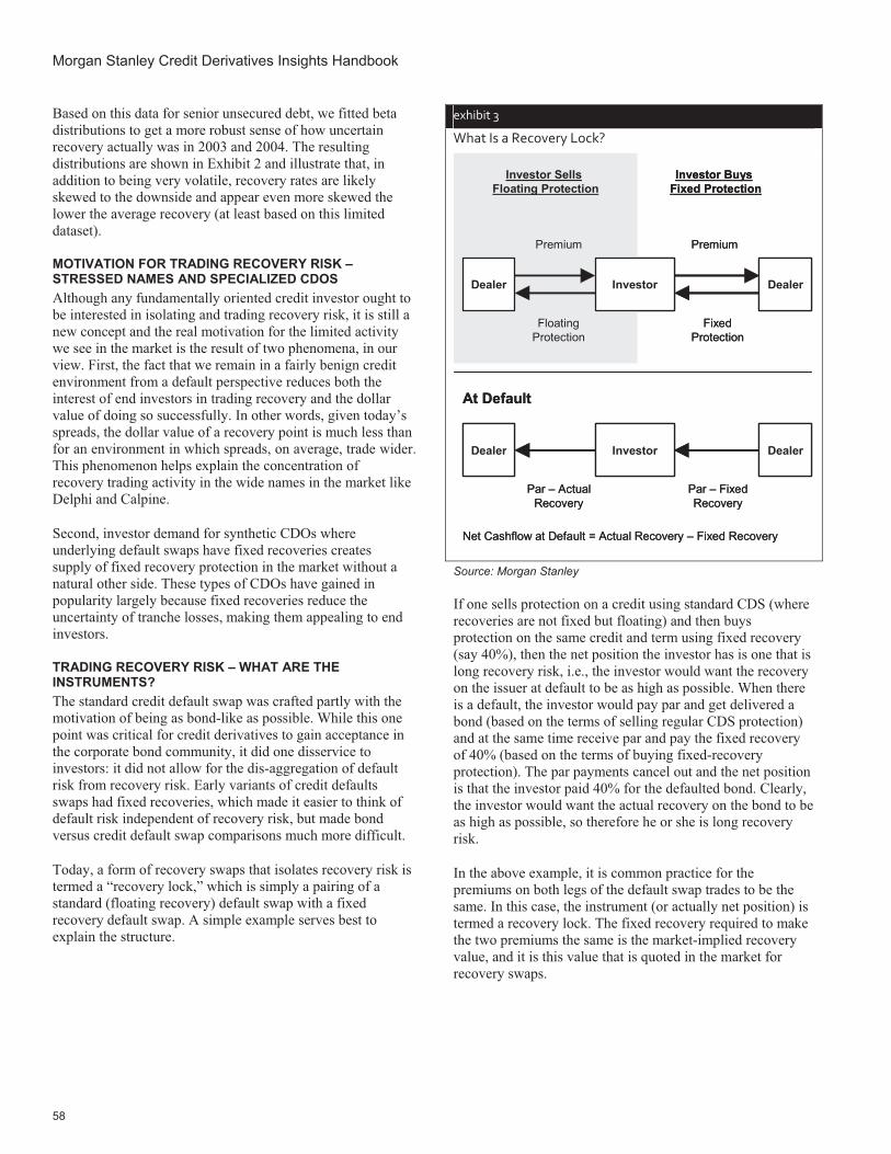
Morgan Stanley Credit Derivatives Insights Handbook
58
Based on this data for senior unsecured debt, we fitted beta distributions to get a more robust sense of how uncertain recovery actually was in 2003 and 2004. The resulting distributions are shown in Exhibit 2 and illustrate that, in addition to being very volatile, recovery rates are likely skewed to the downside and appear even more skewed the lower the average recovery (at least based on this limited dataset).
MOTIVATION FOR TRADING RECOVERY RISK – STRESSED NAMES AND SPECIALIZED CDOS Although any fundamentally oriented credit investor ought to be interested in isolating and trading recovery risk, it is still a new concept and the real motivation for the limited activity we see in the market is the result of two phenomena, in our view. First, the fact that we remain in a fairly benign credit environment from a default perspective reduces both the interest of end investors in trading recovery and the dollar value of doing so successfully. In other words, given today’s spreads, the dollar value of a recovery point is much less than for an environment in which spreads, on average, trade wider. This phenomenon helps explain the concentration of recovery trading activity in the wide names in the market like Delphi and Calpine.
Second, investor demand for synthetic CDOs where underlying default swaps have fixed recoveries creates supply of fixed recovery protection in the market without a natural other side. These types of CDOs have gained in popularity largely because fixed recoveries reduce the uncertainty of tranche losses, making them appealing to end investors.
TRADING RECOVERY RISK – WHAT ARE THE INSTRUMENTS? The standard credit default swap was crafted partly with the motivation of being as bond-like as possible. While this one point was critical for credit derivatives to gain acceptance in the corporate bond community, it did one disservice to investors: it did not allow for the dis-aggregation of default risk from recovery risk. Early variants of credit defaults swaps had fixed recoveries, which made it easier to think of default risk independent of recovery risk, but made bond versus credit default swap comparisons much more difficult.
Today, a form of recovery swaps that isolates recovery risk is termed a “recovery lock,” which is simply a pairing of a standard (floating recovery) default swap with a fixed recovery default swap. A simple example serves best to explain the structure.
exhibit 3
What Is a Recovery Lock?
Investor Sells
Floating ProtectionInvestor Buys
Fixed Protection
Premium Premium
FloatingProtection
FixedProtection
At Default
Par – ActualRecovery
Par – FixedRecovery
Net Cashflow at Default = Actual Recovery – Fixed Recovery
InvestorDealer Dealer
InvestorDealer Dealer
Investor Sells Floating Protection
Investor Buys Fixed Protection
Premium Premium
FloatingProtection
FixedProtection
At Default
Par – ActualRecovery
Par – FixedRecovery
Net Cashflow at Default = Actual Recovery – Fixed Recovery
InvestorDealer Dealer
InvestorDealer Dealer
Source: Morgan Stanley
If one sells protection on a credit using standard CDS (where recoveries are not fixed but floating) and then buys protection on the same credit and term using fixed recovery (say 40%), then the net position the investor has is one that is long recovery risk, i.e., the investor would want the recovery on the issuer at default to be as high as possible. When there is a default, the investor would pay par and get delivered a bond (based on the terms of selling regular CDS protection) and at the same time receive par and pay the fixed recovery of 40% (based on the terms of buying fixed-recovery protection). The par payments cancel out and the net position is that the investor paid 40% for the defaulted bond. Clearly, the investor would want the actual recovery on the bond to be as high as possible, so therefore he or she is long recovery risk.
In the above example, it is common practice for the premiums on both legs of the default swap trades to be the same. In this case, the instrument (or actually net position) is termed a recovery lock. The fixed recovery required to make the two premiums the same is the market-implied recovery value, and it is this value that is quoted in the market for recovery swaps.

Section A, Chapter 6 Trading Recovery Risk – The Missing Link
59
exhibit 4
Fitted Recovery Distribution (Calpine and GM Co.)
0%
10%
20%
30%
40%
50%
60%
0 - 5 5 - 15 15 - 25 25 - 35 35 - 45 45 - 55 55 - 65 65 - 75 75 - 85 85 - 95 95 - 100Recovery Rate (%)
ProbabilityCalpine
GM Co.
Source: Morgan Stanley
THINKING INSIDE THE RECOVERY BOX While the ability to trade and hedge recovery risk is indeed one step in the direction of solving the missing link in credit analysis, recovery risk ultimately needs to be modeled just like default risk. If we combine the notion that recovery values are volatile (Exhibits 1 and 2) with recovery values that we observe in recovery swaps, we can measure the uncertainty of recovery values in a given credit.
When we consider fixed versus floating instruments, one concept that jumps out at us is the idea that taking default risk with fixed recovery should generate less premium than
taking the same risk with uncertain recovery, assuming the fixed recovery is set at the correct level. What the current market for recovery locks gives us is that correct level, since the strike spread and maturity on both the fixed and floating leg are generally the same.
This happenstance gives us the ability to compare the risk associated with floating CDS (with their uncertain cashflows in default) and fixed CDS (with their certain cashflows in default). Conceptually, if we can come up a way to weight the various floating recovery scenarios, then we can isolate the default component of the risk and gain some insight into how investors think about recovery risk. In Exhibit 4, we demonstrate this uncertainty associated with recovery for two credits, combining market pricing on standard CDS, recovery locks and our results for the distribution of Moody’s recovery rates.
RECOVERY ANALYSIS IS THE MISSING LINK While the current overall credit environment is not necessarily ripe for the development of a robust recovery swap market, there is potential for this space to expand in the more stressed corners of the credit markets, as we are beginning to witness now. Despite the simplicity of recovery locks, recovery risk itself is a whole dimension in the credit analysis puzzle that today is meshed with default risk in market standard instruments, like bonds and traditional default swaps. Recovery instruments will help to isolate these risks, but the market is still in need of development.

Morgan Stanley Credit Derivatives Insights Handbook
60
Chapter 7
Floating a New Idea – CMCDS January 21, 2005
Sivan Mahadevan
Much of the development that resulted in today’s standard credit default swap contract was driven by definitions of credit events, sparked, in turn, by the many bankruptcies, defaults and restructurings that the investment grade market experienced during the past credit cycle.
The development of and liquidity injection into the credit curves is still a relatively recent phenomenon (over the past 15 months or so). Active credit curves are important inputs into pricing instruments like credit options and constant maturity credit default swaps. Additionally, from an investor’s perspective, there is little dispersion in the market place today, particularly in investment grade, where spread compression is even higher than it was in 1997 (see “Couch Potato Prognosticating,” January 14, 2005). Tight spreads and a lack of differentiation create a natural reach for yield phenomenon, but also causes concern among those who must be fully invested and don’t feel great about the upside potential.
We rarely discuss very new credit derivatives instruments in our research, partly because until we see some indication of liquidity potential, it is difficult to determine strategic opportunities. However, many market participants have recently asked about one new variant in particular – constant maturity credit default swaps (CMCDS).
As a result, we focus this chapter on ideas involving CMCDS, an instrument that provides investors with a convenient way to string together a series of forward credit curve trades. We feel that varying risk premiums along the credit curve, combined with the potential for spread regime shifts, can result in impractical forward spreads. We can therefore think of CMCDS as a convenient (and positive carry) means to lean against the forwards.
CMCDS MECHANICS A constant maturity credit default swap is a default swap where the premium is reset (on a quarterly basis) to equal a fixed percentage (called the participation rate) of the then-prevailing premium of a plain-vanilla default swap for a certain term. While this is very much a developing market, a typical CMCDS trade today has a 5-year term and references a fresh 5-year default swap every quarter during that 5-year term. Assuming a 50% participation rate, the seller of CMCDS protection would receive 50% of the prevailing premium on a 5-year default swap every quarter, until the
CMCDS expires (in five years) or until a credit event occurs (see Exhibit 1). Consequently, if spreads widen, the quarterly payment would also increase and the concomitant mark-to-market impact could be significantly lower than a regular default swap. The premium on a 5-year default swap is inferred from the market, generally by some type of a fixing process on the reset date by a calculation agent. There can also be a cap on the premium, usually at stressed premium levels.
exhibit 1
CMCDS – Sample Quarterly Premium Calculation
Notional $10,000,000Participation Rate 50%
Quarter 5 Yr CDS
Spread (bp)CMCDS
Spread (bp) Quarterly
Payment ($)1 100 50 12,5002 125 62.5 15,6253 150 75 18,7504 120 60 15,0005 100 50 12,500 Source: Morgan Stanley
PRICING – DETERMINING THE PARTICIPATION RATE Since the protection provided by a CDS and a CMCDS is essentially identical in case of a default, the pricing of the two instruments should be directly linked, as well. Said differently, buyers of protection in either instrument should expect to spend the same amount for the protection at the inception of the contracts. This linkage is enforced through the concept of a participation rate.
We start by using an analogy from the world of interest rate swaps. The fair fixed rate on a swap is the one that equates the present value of floating leg cash flows to the present value of fixed leg cash flows. Employing the same heuristic, the fair participation rate is the rate that equates the present value of payments of a regular CDS to the present value of CMCDS payments.
To determine the expected payments of a CMCDS, we need the implied forward CDS rates, just as we need forward Libor rates to calculate the fixed rate in the case of interest rate swaps. Once we have forward rates, we can determine the participation rate that generates cash flows with a present value matching a plain-vanilla CDS.

Section A, Chapter 7 Floating a New Idea – CMCDS
61
exhibit 2
IG CDX Spot and Forward Curves
(bp)
0
20
40
60
80
100
120
1 2 3 4 5CDS Term (years)
Current 1 Yr Fwd3 Yr Fwd 5 Yr Fwd
Source: Morgan Stanley
INTUITIVE FEEL There are effectively two ways one can think of CMCDS. First, as we mentioned above, CMCDS is a convenient way to string together a series of forwards. If the curve shape and spread levels implied by forwards are realized over the term, the CMCDS and CDS should have the same return at maturity, and this is the basis for pricing. Thus, a position in CMCDS (versus one in CDS) is a way of expressing the view that the forwards will not be realized. Second, ignoring forwards for the moment, CMCDS is really just a floating rate instrument, but the credit premium is what actually floats, as there is no interest rate. A floating premium can have more muted mark-to-market volatility than a fixed premium instrument.
STRATEGIES AND HORIZON ANALYSIS From a strategic perspective, the most interesting aspect of CMCDS is that it separates default risk from spread risk; these are packaged together in more traditional instruments, such as bullet bonds and CDS. This characteristic allows takers of risk to be paid a premium for exposure to default risk, while avoiding exposure to the market risk associated with spread movements. Given the pricing techniques we discussed above, we thought it would be worthwhile to examine how a CMCDS would perform against a bullet CDS under a variety of scenarios.
While the CMCDS does not have any direct exposure to spreads, the realized and implied spreads in the future can have an impact on the price of the swap. We highlight the performance of both a bullet 5-year CDS and a 5-year CMCDS for several scenarios 1 year forward (see Exhibit 3, where pricing is model-based). The first point to note is that price movements are less muted in CMCDS (compared to CDS) across all of the scenarios, but there is still some price volatility. Second, of the scenarios we chose, CMCDS outperforms CDS only in the case where spreads move wider than implied by the forwards. Part of the underperformance
can be attributed to the fact that the floating premium on the CMCDS starts out lower than the CDS level. It should be noted that the floating premium is also expected to increase well above the initial CDS level as time passes.
exhibit 3
Muted Price Movements – CMCDS vs. CDS (One Year Forward)
-2.0%
-1.5%
-1.0%
-0.5%
0.0%
0.5%
1.0%
1.5%
Forwards Realized Curve Unchanged Wider thanForwards
Tighter thanForwards
Bullet CDS
CMCDS
Source: Morgan Stanley
To explain this sensitivity, consider the simple example of a world with perfectly flat credit curves. In this world, the participation rate on a CMCDS would be 100%. As the curve gets steeper, the “fair” participation rate will decline. A CMCDS struck in a flat curve environment should thus appreciate slightly if a steeper curve environment ensues.
PLAYING CREDIT CURVE SHAPE This sensitivity to credit curve shape leads to interesting implications for price sensitivity. Given a credit curve, we can distinguish between a parallel shift and a steepening or flattening to the same 10-year level. In Exhibit 4, we show the price sensitivity of a 5-year CDS to spread moves and a 5-year CMCDS to parallel shifts in the credit curve, as well as to flattening/steepening. Under some scenarios, these moves can offset one another to a large extent. For example, the negative impact of increased spread levels, which imply increased default risk, makes the CMCDS marginally less valuable. This can be offset if the shift is accompanied by a steeper curve, implying larger floating coupon payments as the instrument reaches maturity, which increases the value. Which one dominates will depend largely on the magnitude of the relative changes.

Morgan Stanley Credit Derivatives Insights Handbook
62
exhibit 4
CDS and CMCDS Spread and Curve Exposures (Price Sensitivity of $10MM 5 Year Positions)
-6,000 -5,000 -4,000 -3,000 -2,000 -1,000 0 1,000 2,000 3,000
5 Year Bullet DV01 (Wider)
PV of Parallel 01 Shift (Wider)
PV of 01 of Curve Steepness
PV of Wider Spread with Steepening
Bullet CDS
CMCDS
Source: Morgan Stanley
WHO ARE THE NATURAL BUYERS AND SELLERS? Right now, there are not many of either, and there may never be. Yet, as we saw above, the risk and return implications of CMCDS are significantly different from CDS in many scenarios (except when the forwards are realized) so it is indeed worth considering who might benefit from buying or selling CMCDS protection. In the current credit curve environment, the seller of protection gives up quite a bit of current premium, but could have less mark-to-market volatility and will outperform CDS when spreads go wider than implied by the forwards. For those who must be invested, but have a negative view on credit (over and above what is implied by forwards), selling CMCDS protection would be beneficial. It is also a simple way of implementing the view that default risk is benign, but spread levels are not very exciting (which fits our view, see “Breaking Down the Barriers,” December 17, 2004). Long/short strategies in tranches can also implement this view, but can be more complicated in nature.
The natural buyer of CMCDS protection is perhaps more straightforward, given that lower current premiums might seem appealing. For any protection buyer who feels that the forwards overstate spread widening over the term, buying CMCDS protection on its own would be more attractive than CDS protection itself. In either case (buyer or seller), lower potential mark-to-market volatility of CMCDS may be appealing to investors who value the lower volatility, or who must treat cash and derivative instruments differently.
SOME PRACTICAL ISSUES For investors who are excited about the convenience of packaging forwards into a single instrument, and the resulting different risk and return characteristics (compared to traditional CDS), we caution that these instruments are still relatively nascent. Transaction costs and the potential that market prices can drift away from model-based valuations are important practical implications (consider how correlation skew has moved with spread levels). Also, while the cap in CMCDS is generally deep out of the money at inception, the pricing of this cap as stress enters a particular credit can be somewhat subjective, as well.
What little activity we have seen in the market for CMCDS has been centered around the benchmark indices, rather than individual credits. One debate in the market has focused on how to treat the index roll. From a risk-management perspective, we find it simpler to think of a CMCDS on an index to always be based on today’s composition of the index; however, as indices roll and become off-the-run, it may prove difficult to apply a fixing process to levels on an off-the-run index. As a result, some market participants have proposed that, as the index rolls, the CMCDS should refer to the new index, which leaves the CMCDS users exposed to changes in index constituents. In any event, what we find interesting about this instrument is its vastly different risk and return profile, which can encourage investors to think outside of the box.

63
Chapter 8
Understanding Corporate Bond Options – Valuation Issues and Portfolio Applications June 11, 2003
Sivan Mahadevan
INTRODUCTION Options on corporate bonds, the right to buy or sell a bond at the strike price during a specific period, were among the earliest credit derivative instruments in the credit markets. Most outstanding corporate bond options are embedded in corporate bonds and are thus implicitly held by either bond issuers (for call options) or bond investors (for put options). As the market for separately traded corporate bond options develops, we focus our research efforts on understanding their investment characteristics, application in credit portfolios and valuation.
The corporate bond options that trade in the secondary market are typically sourced from simple structured credit transactions in which investors, issuers or underwriters write options on bonds to create desired investment characteristics or additional yield. The options are then redistributed and traded in the secondary market. Examples of structured credit transactions that result in new options written include:
� Repackagings of corporate bonds into trusts, in which end investors write call options for additional yield and reductions in average life
� Repackagings of putable corporate bonds into bullet securities, in which the investor would sell a call option with an exercise date equal to the exercise date of the embedded put option
� Writing of at-the-money options by investors who want to protect gains made in bullet securities prior to a rising rate environment (writing covered calls)
It is important to note a few points with respect to outstanding options. First, while corporate issuers are the largest holders of call options on corporate bonds, they typically do not redistribute this risk, although in theory they could. Issuers who hold call options may not exercise them whenever it makes economic sense (i.e., they may not act as rational market participants in the academic sense). The reasons for this behavior may include corporate capital structure issues, funding costs and liquidity in the primary markets. End investors who hold options will likely act more rationally, in the academic sense.
In this chapter we first explore the investment characteristics of corporate bond options, discussing both portfolio applications and trading strategies. We then propose a valuation framework based on traditional swaption market practices but taking into consideration differences in volatility and the likelihood of default. We conclude with some discussion of practical issues for investors that may affect how investors can incorporate these instruments into portfolios to help achieve investment objectives.
Investment�Characteristics,�Portfolio�Applications�and Trading Strategies Since callable corporate bonds are a common instrument in the credit markets (5% of index-eligible investment grade corporate bonds are callable, representing $55 billion of debt), we begin our discussion of corporate bond options with a comparison of the price sensitivity of a bullet bond with that of a callable bond with the same terms. In Exhibit 1 we show the price changes relative to yield changes for a bullet bond with a 30-year maturity, along with those of a similar instrument that is callable after three years. The holder of a callable bond (who has written a call to the issuer) effectively gives up the positive performance of the highlighted region when compared to the performance of the bullet security.
exhibit 1
The Call Option Region
Price
60
80
100
120
140
160
180
200
1.75
2.25
2.75
3.25
3.75
4.25
4.75
5.25
5.75
5.95
6.15
6.35
6.55
6.75
6.95
7.15
7.35
7.55
7.75
7.95
Yield
30 Yr Bullet 30 Yr NC 3
Option Value
Source: Morgan Stanley

Morgan Stanley Credit Derivatives Insights Handbook
64
This highlighted region is the option payout diagram (shown in isolation in Exhibit 2) for the owner of the call option, which is an extremely convex instrument. The option is also very sensitive to changes in rates, implying that it has both a long interest rate and spread duration.
exhibit 2
Call Option Isolated: Convexity and Duration
Price
-10
0
10
20
30
40
50
60
70
80
1.75
2.25
2.75
3.25
3.75
4.25
4.75
5.25
5.75
5.95
6.15
6.35
6.55
6.75
6.95
7.15
7.35
7.55
7.75
7.95
Yield
Option Value
Source: Morgan Stanley
PORTFOLIO APPLICATIONS: DURATION AND CONVEXITY At a time when traditional corporate bond portfolio managers are beginning to explore the application of nontraditional instruments such as credit default swaps, baskets and CDO tranches in portfolios, we suggest adding corporate bond options to this list of novel tools. In fact, corporate bond options are likely more “traditional” than the others, given that nearly every asset-liability or total return portfolio already has short exposure to call options through callable bonds.
In a nutshell, call options are instruments that are much more sensitive to interest rate (and spread) changes than bonds. As such, their high duration and convexity characteristics can be beneficial to investors seeking to adjust interest rate and spread sensitivity in portfolios. Investors can view corporate bond options as a tool with duration and convexity “leverage” to help achieve portfolio goals. We discuss the application of both below.
DURATION EXTENSION Portfolio managers may choose to increase the duration of their portfolios to match benchmarks or implement active views. At the asset allocation level, our Global Pension Group has done extensive research showing that a significant increase in the dollar duration of fixed income portfolios is necessary to optimally fund defined benefit pensions.1 Since this seminal work, many public and private pension funds have reworked their asset allocation schemas in an asset-liability framework (as opposed to an asset-only framework), which has generally resulted in extending the duration of their fixed income portfolios. To implement these duration extension programs, portfolio managers have considered a variety of long-duration interest rate products (e.g., zero coupon bonds or Treasury futures overlays), and we believe that corporate bond options can be used for similar reasons.
WHY CONVEXITY? PROTECTING PORTFOLIOS AT THE TAILS Why is convexity a good attribute to have in a portfolio? Simply put, a positively convex instrument benefits portfolios during extreme movements in interest rates or spreads. When portfolios are interest rate hedged versus their liabilities or benchmarks, convexity (or excess convexity) can provide a substantial return cushion at the tails of the interest rate or spread distributions. We view this as being a natural use of positively convex instruments in corporate bond portfolios; but adding convexity generally comes at a cost (less yield for a given duration).
Furthermore, it is important to note that many fixed income portfolios have negatively convex instruments (e.g., mortgages) or instruments that are only slightly positively convex (e.g., callable corporate bonds), which can result in significant underperformance versus benchmarks or mismatches versus liabilities at the tails of the distributions. We are living in one such tail environment today (see Exhibit 3): the options written by many callable bond investors are significantly in-the-money to issuers, resulting in a large cost to many portfolios. Positively convex instruments can be used to offset some of this risk.
A bullet bond has positive convexity, something most fixed income investors learned their first day on the job. As the graph in Exhibit 2 illustrates, on a relative basis the positive convexity of a call option is significantly greater than that of the long-dated bullet bond in a falling interest rate environment. However, the bullet bond’s price sensitivity is positively convex at the other extreme as well, whereas the option’s value is flat (zero convexity) at that extreme. How can investors use call options to create truly convex instruments in all interest rate and spread environments?
1“Asset Liability Management Within A Corporate Finance Framework,” Morgan Stanley Global Pension Quarterly, July 1998.

Section A, Chapter 8 Understanding Corporate Bond Options – Valuation Issues and Portfolio Applications
65
exhibit 3
The Tails of Interest Rates (40-Year History)
Frequency
0
5
10
15
20
25
30
35
40
1.0 2.0 3.0 4.0 5.0 6.0 7.0 8.0 9.0 10.0 11.0 12.0 13.0 14.0 15.0Yield
2 Year Yields
Current Environment
Frequency
0
10
20
30
40
50
60
1.0 2.0 3.0 4.0 5.0 6.0 7.0 8.0 9.0 10.0 11.0 12.0 13.0 14.0 15.0Yield
5 Year Yields
CurrentEnvironment
Frequency
0 10 20 30 40 50 60
1.0 2.0 3.0 4.0 5.0 6.0 7.0 8.0 9.0 10.0 11.0 12.0 13.0 14.0 15.0Yield
10 Year Yields
Current Environment
Source: Morgan Stanley
PORTFOLIO APPLICATION I: THE CONVEXITY BARBELL In Exhibits 4-7 we show an example that is very applicable in today’s interest rate environment. The fundamental premise is that a premium bond is more convex than a duration equivalent par bond (all else being equal) in a rallying interest rate environment but less convex in a rising interest rate environment (Exhibit 4). Investors can combine a par bond with a call option and create an instrument that has equivalent duration but is truly more convex than the premium bond alone.
exhibit 4
Convexity Comparison: Equal Duration Premium and Par Bonds
P/L ($MM)
-4
-2
0
2
4
6
8
10
1% 2% 3% 4% 5% 6% 7% 8% 9% 10%Yield
Premium Bond Par Bond
Source: Morgan Stanley
In Exhibit 5 we show two hypothetical examples in which the investor sells a premium bond to buy a par bond and an in-the-money option on the premium bond.
The first trade is structured to be both duration and proceeds neutral, but has a give-up in yield of 72 bp in exchange for the pickup in convexity based on our fair value approximation for the option. This trade structure is effectively a convexity barbell. Note, however, that anomalies can exist, given the relatively nascent market for traded corporate bond options, that may make a transaction like this more attractive from a yield perspective.

Morgan Stanley Credit Derivatives Insights Handbook
66
exhibit 5
The Convexity Barbell: Two Hypothetical Trades
Size ($MM) Security Coupon Price Yield to Mat Eff Dur Eff Convx
Proceeds ($MM)
Sell 10.0 23-Year Premium Bond 6.00% 112.15 5.11% 13.2 244.8 11.5Buy 10.4 13-Year Par Bond 4.75% 100.71 4.68% 9.6 114.7 10.8Buy 5.7 Call Option: 3.5-Yr Exp, 100 Strike on 23-Year Bond -- 12.62 -- 65.8 3988.1 0.7Diff -- -0.72% 0.0 357.3 0.0 Sell 10.0 23-Year Premium Bond 6.00% 112.15 5.11% 13.2 244.8 11.5Buy 10.0 13-Year Par Bond 4.75% 100.71 4.68% 9.6 114.7 10.3Buy 5.5 Call Option: 3-Yr Exp, 100 Strike on 23-Year Bond 12.62 65.8 3988.1 0.7Diff -0.86% 0.0 357.3 0.5 Source: Morgan Stanley
As structured, the trade’s convexity advantage is illustrated in Exhibit 6 (which shows total return at option maturity for changes in yield). The yield give-up results in underperformance over a wide range of yield distributions (approximately 250 bp), which investors could view as a large price to pay for convexity.
exhibit 6
The Convexity Barbell: Sell Premium Bond, Buy Par Bond/Options Package (Duration and Proceeds Neutral)
P/L ($MM)
-3
-2
-1
0
1
2
3
4
5
6
7
8
2% 3% 4% 5% 6% 7% 8% 9% 10%Yield
Premium Bond Par Bond/Option Pkg (Dur,Proceeds Neutral)
Underperformance from Yield Give Up
Source: Morgan Stanley
A second alternative is to take cash out of the transaction. In Exhibit 5, we show a second example trade, in which we fix the par amount of the par bond to be equal to that of the premium bond and adjust the option notional amount until the trade is duration equivalent. This structure results in a sharper barbell without any underperformance region, assuming the option is valued at our fair value approximation (see Exhibit 7).
exhibit 7
The Convexity Barbell: Sell Premium Bond, Buy Par Bond/Options Package (Duration Neutral, Take Out Cash)
P/L ($MM)
-3
-2
-1
0
1
2
3
4
5
6
7
8
2% 3% 4% 5% 6% 7% 8% 9% 10%
Yield
Premium Bond Par Bond/Option Pkg (Dur Neutral, Cash Out)
Source: Morgan Stanley
Note that while the example trades are duration neutral, they do express a yield curve view, which is not depicted in the P/L graphs above, as yield changes are assumed to be parallel. In particular, given the sale of a long-dated bond to buy a shorter-dated bond, curve flattening would hurt the trade while curve steepening would benefit the trade. The option’s value is independent of curve shape.

Section A, Chapter 8 Understanding Corporate Bond Options – Valuation Issues and Portfolio Applications
67
PORTFOLIO APPLICATION II: WRITING COVERED CALLS Another application of bond options that is relevant in today’s environment is the idea of writing covered calls on premium priced bullet bonds. This structure can be a means to monetize the intrinsic value generated in a long-duration instrument after a rally in rates as well as any value attributable to the volatility of rates in the future. The structure can be used to express a view that rates will be relatively unchanged to higher in the future. The structure is equivalent to selling a premium bond to buy a callable bond of the same issuer and term and realizing the difference in price as a gain.
Consider the situation of the 23-year premium bond in Exhibit 5. Because of its long duration and convexity, this bond will depreciate quickly in an environment of rising rates. One way to protect the value in this instrument without giving up current yield is to sell a call option on the bond struck at the at-the-money yield.
Exhibit 8 illustrates the advantage of this structure (a combination of the premium bond and written call option) over holding the long-dated premium bond alone. For widening of rates up to approximately 6%, the covered call strategy effectively immunizes the position from interest rate movements and hence performs better than the bond alone. For a widening of rates in excess of 6%, the strategy continues to outperform by a fixed amount driven by the option premium received at inception of the trade. The covered call strategy clearly underperforms if the yield on the bond falls below this, much like the performance of a callable bond.
exhibit 8
Covered Calls – Monetizing Volatility
-6
-4
-2
0
2
4
6
8
10
12
1% 3% 5% 7% 9% 11% 13% 15%Bond Yield At Option Maturity
Premium Bond TR Package TR
Source: Morgan Stanley
The above examples are two of numerous applications whereby investors can use the duration and convexity of corporate bond options to alter the interest rate and spread sensitivity of fixed income portfolios to meet investment objectives.
TRADING STRATEGIES – ISOLATING THE COMPONENTS OF RISK While many investors will find value in long or short option positions within their credit portfolios, other investors may wish to isolate certain aspects of corporate bond option risks to express particular views. We break the factors that drive the pricing of corporate bond options into five components, namely credit volatility, credit risk, interest rate volatility, interest rate risk, and interest rate and credit spread correlation (see Exhibit 9, left side).
While asset-liability and total return-oriented investors may desire all five risks, given the goal of matching or outperforming benchmarks or liability schedules, other investors may wish to isolate and/or mitigate one or more of these risks to achieve investment objectives.
In Exhibit 9 (right side) we show the instruments that can be used to hedge these risks, from which we can derive trading strategies as shown in Exhibit 10. Investors can use these strategies to express views on a company without being forced to implement an explicit view on interest rates (or volatility of rates) or credit risk.
exhibit 9
Components of Risk and Hedging Instruments
NoneInterest Rate and Credit Spread Correlation
Credit Spread OptionCredit Volatility
SwaptionInterest Rate Volatility
Default SwapCredit Risk
Corporate Bond
Interest Rate Swap
Interest Rate Risk
Hedging InstrumentsComponents of Risk
NoneInterest Rate and Credit Spread Correlation
Credit Spread OptionCredit Volatility
SwaptionInterest Rate Volatility
Default SwapCredit Risk
Corporate Bond
Interest Rate Swap
Interest Rate Risk
Hedging InstrumentsComponents of Risk
Source: Morgan Stanley

Morgan Stanley Credit Derivatives Insights Handbook
68
exhibit 10
Corporate Bond Option Trading Strategies Trading Strategy Package Rationale Long credit volatility Long option, long credit protection, short
swaption, pay fixed in swap Pure long credit volatility play; expresses a view that
company’s valuation becomes markedly less certain
Long credit volatility and credit risk Long option, short swaption, pay fixed in swap
A levered long credit position; implements a view that company rallies strongly
Long credit and interest rate volatility, credit risk
Long option, pay fixed in swap Option position without interest rate risk; expresses view that company does well independent of economic cycle
Long credit and interest rate volatility Long option, long credit protection, pay fixed in swap
Pure long credit and interest rate volatility play; implements an “uncertain” economic view on a cyclical or interest rate sensitive company
Long credit and interest rate volatility, interest rate risk
Long option, long credit protection Option position without credit risk; expresses an increasingly uncertain credit view combined with a view on rates
Long credit volatility and interest rate risk Long option, long protection, short swaption Expresses a weak-economy view combined with increased credit uncertainty
Long credit and interest rate risk, credit and interest rate volatility
Long option Original option position with duration and convexity applications
Source: Morgan Stanley

Section A, Chapter 8 Understanding Corporate Bond Options – Valuation Issues and Portfolio Applications
69
Valuing Corporate Bond Options There are several variants to traditional option pricing models that are used to price fixed income options. The most liquid market by far is the swaption market, which we suggest using as both a frame of reference and a source of implied volatility in corporate bond option valuations. The holder of a swaption has the right to enter into an interest rate swap on a specified date (European option) or a range of dates (American or Bermudan option).
There are two components of the valuation process for a call option on a corporate bond that differ from the valuation of options on a credit risk-free instrument like an interest rate swap. First, the volatility input must take into consideration the volatility of the credit risk (in addition to the interest rate risk), and second, a scenario in which the issuer defaults prior to option maturity must be factored in as well. We address both issues in this section, building on a swaption valuation framework, and provide some pricing examples as well. While much research has been published on understanding the valuation of options related to fixed income instruments, research discussing options on credit risky instruments has been more recent. We refer readers to Duffie and Singleton 2003 for a more detailed analysis.2
THE RELATIONSHIP OF INTEREST RATES AND CREDIT SPREADS Given that the secondary market for corporate bond options is still developing, it is difficult to observe implied volatility; therefore, appropriate volatility inputs to option pricing models must be derived by other means. An approach we suggest is to observe implied volatility in the swaption market and then “add in” volatility from credit markets based both on historical spread volatility and the correlation of spreads with swap rates. Given an adjustment for correlation, we assume that these two volatility measures are indeed additive. Default is modeled separately below.
To get a better sense of the relationship of interest rates and credit spreads, we observed the historical correlation of credit spreads (over Libor) and swap rates over a 14-year period. In Exhibit 11, we show the results by credit quality, with overall correlation ranging from –31.6% to –38.7%. On a three-year rolling basis, the correlation values are always negative for all three credit quality sectors, and have fallen to as low as –70%.
The overall values are intuitive, given the general sensitivity of corporate credit risk to economic cycles. Both periods of highly negative correlation occur during coinciding periods of stress in both the interest rate and credit spread markets.
2Credit Risk, Duffie, D., and Singleton, K., Princeton University Press, 2003.
exhibit 11
Always Negative – Rolling Correlation of Swap Rates with Credit Spreads
-80%
-70%
-60%
-50%
-40%
-30%
-20%
-10%
0%
Jan-92 Jun-93 Nov-94 Apr-96 Sep-97 Feb-99 Jul-00 Dec-01 May-03
AA A BBB
BBBs – Full Period Corr = -36.7%
As – Full Period Corr = -38.7%
AAs – Full Period Corr = -31.6%
Source: Morgan Stanley, Salomon Analytics
In addition to this correlation, it is useful to observe historical credit spread volatility in formulating an appropriate volatility input into an option pricing model. In Exhibit 12 we show historical volatility over the same period for AA, A, and BBB rated corporate debt. On an absolute basis, the volatility rises with credit quality risk (as we would expect). On a three-year rolling basis, AA and A credits were relatively stable, while the BBB rolling volatility was much more volatile itself, rising to a current level of over 90.
exhibit 12
Rolling Volatility (in bp) of Credit Quality Sectors
0.0
10.0
20.0
30.0
40.0
50.0
60.0
70.0
80.0
90.0
100.0
Jan-
92
Jan-
93
Jan-
94
Jan-
95
Jan-
96
Jan-
97
Jan-
98
Jan-
99
Jan-
00
Jan-
01
Jan-
02
Jan-
03
AA A BBB
BBBs - Full Vol = 53.9
AAs - Full Vol = 23.9
As - Full Vol = 28.5
Source: Morgan Stanley, Salomon Analytics

Morgan Stanley Credit Derivatives Insights Handbook
70
VALUING THE OPTION With this background, we discuss below one method for valuing corporate bond options struck near par, based on the standard Black swaption framework. Given the inherent complexities in valuing American/Bermudan options on bonds, we have concentrated on the issues related to valuing European options here. This valuation could therefore be viewed as a floor on Bermudan or American options. In particular, we focus on three points:
� Determining an expected forward risky rate (or price) at option expiry
� Calculating an appropriate volatility given implied swaption volatility and assumptions for credit spread volatility and correlation
� Modeling the likelihood of default
EXPECTED FORWARD CREDIT RISKY RATE AT OPTION EXPIRATION The prevailing risky rate applicable to a corporate bond at the time of option expiration can be divided into the future prevailing swap rate and the Libor credit spread for the appropriate maturity.
The current forward swap rate can be observed directly from the prevailing swap curve today. We use this forward rate as an approximation of the expected future swap rate.
The expected future credit spread can potentially be derived in a manner similar to that of the swap rate if the credit has instruments with a variety of maturities. Alternatively, one can use current credit spreads to approximate the forward credit spread in a variety of ways. The methodology used and level of rigor with which the future credit spread is derived should weigh the absolute level of spreads and the impact on option valuation. Generally, the wider the credit spread, the greater the impact of the spread assumption on the option valuation.
The expected future credit risky rate can then be computed and utilized in the option valuation.
DETERMINING VOLATILITY Moving from volatility of swap rates to volatility of risky rates within the framework of the Black model is a challenge. In order to make use of the forward looking swap rate volatility data available from the swaption market, we rely on the assumption of lognormal swap rates. However, in order to use the Black framework to value the option on a default risky bond, we rely on the assumption that risky rates are also lognormal.
The method we employ allows us to approximate the expected value and variance of forward credit spreads and to calculate the expected value and volatility for the risky rate. We rely on the assumption that credit spreads are distributed in such a way that when added to a lognormal distribution, the result is once again lognormal.
The variance of the risky rate is derived using the following basic formulation:
adCreditSpreSwapadCreditSpreSwapRiskyRate VVVVV �2���
Where:
)1(22 �� SwapeFV SwapSwap
Swap = swaption implied volatility (generally at the money; can be adjusted for skew)
� = correlation between the level of the swap rate and the level of credit spread
SwapF = Forward swap rate from option expiration through
bond maturity
Finally, the RiskyRate parameter is calculated based on inverting the formula above:
�
� �
��� 12
RiskyRate
RiskyRateRiskyRate F
VLn
Exhibit 13 illustrates the sensitivity of the risky rate volatility (the RiskyRate parameter) for various credit spread and credit spread volatility assumptions for a given swap rate, swap volatility and correlation. We find that for reasonable combinations of credit spread and credit spread volatility, the impact of varying correlation within the range from –10% to –40% results in relatively small changes in volatility for typical investment grade spread levels. Exhibit 14 illustrates the sensitivity of the risky rate volatility across a broad range of correlation for a credit with a spread of 100 bp.

Section A, Chapter 8 Understanding Corporate Bond Options – Valuation Issues and Portfolio Applications
71
exhibit 13
Risky Rate Volatility
(Swap = 5%, Swap� = 15%, ��= -30%) Credit Spread (bp) Credit Spread Standard Deviation (bp) 10 50 100 150 20010 14.3% 13.2% 12.1% 11.2% 10.4%30 14.1% 13.1% 12.0% 11.1% 10.3%50 15.0% 13.9% 12.8% 11.8% 11.0%70 16.8% 15.6% 14.3% 13.2% 12.3%90 19.2% 17.8% 16.3% 15.1% 14.0%110 21.9% 20.4% 18.7% 17.3% 16.1%130 24.9% 23.2% 21.3% 19.7% 18.3%150 28.1% 26.1% 24.0% 22.2% 20.7%170 31.4% 29.2% 26.8% 24.8% 23.1%190 34.7% 32.3% 29.7% 27.5% 25.6%210 37.9% 35.4% 32.6% 30.2% 28.1% Source: Morgan Stanley
exhibit 14
Risky Rate Volatility
(Swap = 5%, Swap� = 15%, Spread = 100)
0%
5%
10%
15%
20%
25%
30%
35%
40%
-90% -80% -70% -60% -50% -40% -30% -20% -10% 0%Correlation
50 bps Spread Volatility 100 bps Spread Volatility 200 bps Spread Volatility
Source: Morgan Stanley
DEALING WITH DEFAULT In order to deal with default risk within this framework, we have made the assumption that the distribution of forward rates at option maturity is conditional on no default occurrence before option expiry.
The probability of default is explicitly incorporated through a default hazard rate, which is built into the discount factors used in the valuation. The hazard rate can be derived from credit default swap or bond spreads using a risk neutral framework or can be readily approximated with the following formulation:
Ht = CDSt /(1- Recovery Rate)
Ht is defined as the annualized default hazard rate applicable throughout the period before option expiry and CDSt is the credit default swap spread for a swap maturing at option expiry. The hazard rate is incorporated into the
our model by modifying the definition of the discount factor PV(0,t) to be e –(r+Ht)*t. The implication of this approach is that the value of the option is zero in default scenarios. For call options with strike prices significantly below par as well as put options, further adjustment to the valuation may be required to reflect the possibility of a positive return on the option in a default scenario.
Conceptually, one can think of the complete distribution of forward risky rates as being comprised of two components, which our approach assumes are independent of one another:
1. The distribution of rates given default does not occur before option expiry and
2. The portion of the distribution due to default occurrence before option expiry
Exhibit 15 illustrates this conceptual framework in the context of bond total returns in 2002.
exhibit 15
The Performance Skew in Investment Grade Credit (2002) Frequency
0
50
100
150
200
250
-30% -26% -22% -18% -14% -10% -6% -2% 2% 6% 10% 14% 18% 22% 26% 30%2002 Total Return Buckets
AddressedthroughDefaultHazard Rate
Addressed through Volatility
Source: Morgan Stanley
The result of this approach is to effectively “discount” the payoff of the option for default occurrence. Therefore, valuations are generally lower than for equivalent default risk-free options. This effect of this discount is minor for short-dated options but can be dramatic for long-dated options.
OPTIONS WITH MORE COMPLEX STRUCTURES Some bond options have additional structural features that make them much more complex to value than standard European options. Characteristics such as multiple exercise dates and varying exercise prices, combined with the nature of bond price dynamics relative to changes in rates, make such features extremely complex to evaluate without moving to a framework in which we generate a complete distribution for the full maturity range of forward rates.

Morgan Stanley Credit Derivatives Insights Handbook
72
While lattice-pricing structures can address some of these issues, an approximate floor can readily be found for complex option values using multiple applications of the methodology presented above. We take advantage of the fact that the value of a complex option with multiple exercise dates must be at least that of a European option exercisable on one of those dates. We construct a portfolio of European options expiring at various points in the exercise period. We value these options based on the methodology above and approximate a floor valuation of the more complex option as the maximum of these.
Through the adjustment of the input parameters we are able to reflect the varying relationship between yield and price volatility at different points in time and the “pull to par nature” of bonds and varying exercise terms through time.
A CLOSED FORM APPROXIMATION While the standard Black swaption model allows for a closed form solution, we use the framework to simulate forward rates and calculate bond prices to derive an option valuation. Relaxing the theoretical framework we have used above, one can derive a closed form approximation by modeling the risky bond forward price directly in a forward price option model (with adjustment for default). The expected yield can be mapped into an expected price and the volatility calculated above can be used to approximate the forward price volatility using an adjustment based on duration of the bond at option expiry. We find that this approximation generally understates value under equivalent assumptions.
Exhibit 16 shows a comparison of the option valuation for the option described in Exhibit 5 based on the forward rate simulation methodology and the forward price closed form approximation. We find that for near at-the-money options (expected forward rates between 4.25% and 6.00% in this case) the closed form underestimates the value of options by 10-12%, with error declining in percentage terms for options heavily in or out of the money.
exhibit 16
Closed Form Approximation
$0
$10
$20
$30
$40
$50
$60
$70
$80
$90
1% 2% 3% 4% 5% 6% 7% 8% 9% 10%
Rate Option Value Forward Option Value
Source: Morgan Stanley
Conclusion – Practical Issues In this chapter we have described attributes of corporate bond options and their application to credit portfolios and presented several trading strategies that investors may find useful to implement views on the market and individual credits. We have also discussed valuation issues in a swaption framework, taking credit-specific risk into consideration. We conclude with a brief summary of some of the practical issues that market participants must address to value and invest in these instruments.
On the valuation front, we have based our proposed valuation framework on a standard European swaption model (Black) with adjustments for credit volatility and default scenarios. However, corporate bond options can be Bermudan- or American-style, which will make options more valuable but also complicates the computation process. European-style option analysis can be used as a “floor” on the valuation for American and Bermudan options. Other bond-level issues can complicate the process as well, as we touched upon in the previous section.
On the topic of determining credit volatility, we believe our approach is theoretically sound; but, in our experience, very few investors who are valuing options today are using this type of approach in practice. As the still-nascent market for corporate bond options develops, we expect valuation techniques to evolve as well.
On the topic of portfolio applications, there may be significant accounting issues for investors hoping to incorporate corporate bond options in portfolios. An institution’s accounting regime will determine how options are treated. Derivative accounting regulations could force mark-to-market for these options (in portfolios that are otherwise not marked to market). The fact that options have no income stream may be an issue as well. Hedge accounting rules may be applicable in situations where short call option positions act as covered calls or where long call option positions are considered hedges against callable bonds. We urge investors to consult their accountants to gain more insight into these accounting issues.

Section B
Valuation and Performance

Morgan Stanley Credit Derivatives Insights Handbook
74
Chapter 9
Libor Metrics June 27, 2003
Sivan Mahadevan Rizwan Hussain Anisha Ambardar
A combination of low spreads, high dollar prices and a steep yield curve has made relative value analyses difficult today, both within the universe of corporate bonds and between bonds and default swaps. Looking at bonds on a Libor basis is supposed to be the common denominator approach, but confusion persists. Using Libor spreads is a bit like the Metric System: everyone agrees that it is better, but it is hard to develop intuition for the measures when the market trades on Treasury spread and dollar price.
We focus on describing the various Libor spread measures in simple terms, recommend using the intuitive Z-Spread approach for relative value purposes (for both cash investors and derivatives users), and show some practical examples to illustrate relative value in an environment where a handful of basis points really matter.
FOUR LIBOR MEASURES There are four Libor spread measures commonly used by market participants. Par and market value asset swaps are meant to be used by those doing real asset swaps (i.e., converting a fixed rate bond to a floating rate instrument), while interpolated swap curve spreads and Z-Spreads are relative value measures used by those who are focusing on fixed rate assets.
exhibit�1�
Par�Asset�Swap�–�8%�10-Year Bond Priced at $110
0 3 6 120Months
110
4
F F F
4
10
4
104
Investor
Bond
Swap Counterparty
Notional Amount = 100
Note: The floating payment F equals Notional Amount*(LIBOR +
Spread) / 4. Source: Morgan Stanley
ASSET SWAPS A par asset swap is the most common type of fixed-for-floating swap used by credit investors. If a bond trades at par, then the swap simply involves an exchange of coupon
payments for floating rate Libor plus a fixed spread. When a bond trades at a premium, the swap becomes off-market, and there is typically an upfront payment from the swap counterparty to the investor to make up for the premium (see Exhibit 1).
A market value asset swap is less common and involves converting the fixed-rate bond into a floating-rate note with par equal to the original bond’s dollar price.
MAKING UP FOR UNACCOUNTED CREDIT RISK While asset swaps are practical vehicles for converting fixed-rate bonds to floating-rate, the “spread” over Libor paid out by the swap counterparty is not necessarily an accurate measure of the bond’s credit risk, particularly when there are upfront or residual payments.
In a par asset swap, the present value of all the periodic cash flows is equal to the premium or discount on the bond. This present value is calculated using the Libor term structure, while the premium on the bond is a result of cash flows, which are discounted using a credit-risky rate. As a result, asset swap spreads reflect the shape of the Libor yield curve but fail to fully incorporate the impact of the credit-risky nature of the bond cash flows. This mismatch in discount rates introduces a bias in the asset swap spreads, which is particularly acute for bonds with significant premiums or discounts and bonds with wide credit spreads. One point we want to make clear is that asset swaps are not incorrectly measuring credit risk. Indeed, the swap itself has no credit exposure (to the bond issuer) because all of the payments on the swap are due whether or not the bond defaults prior to maturity.
GOING BACK TO BASICS For investors who are simply using Libor measures to make relative value decisions between bonds and/or default swaps, we consider two other measures more relevant. Both measures involve a common and intuitive practice, namely comparing a bond’s yield or cash flows to a benchmark. An interpolated swap spread is one measure and is simply the yield to maturity of a bond minus the interpolated yield on the swap curve. This spread is termed I-Spread (or yield-on-yield spread by asset swappers).
I-Spread ignores the shape of both the Libor yield curve and the credit curve, and thus does not reflect any impact for the actual timing of payments. Two bonds with the same maturity and yield but different coupons (and thus different duration) would get the same I-Spread. The second measure involves an OAS model. If we take a step back and think about bond basics, what investors require is a method to compare a series of risky cash flows to a risk-free yield curve

Section B, Chapter 9 Libor Metrics
75
that is not biased by dollar prices and coupons. An OAS model, using a zero Libor curve can solve this problem. However, OAS models build a tree of paths, adding unnecessary complexity to a relatively simple problem.
CONVERGING ON Z-SPREAD An OAS model with a zero volatility input can reduce the tree to a simple yield curve, which results in an intuitive price/yield type of calculation. Under this method, we calculate a fixed spread over a series of zero-coupon Libor rates that equates the price of the bond with the present value of the cash flows. We call this spread the Z-Spread, which one can think of as zero-volatility Libor OAS. Z-Spread may be easier to explain as an equation than in words. The general price/yield relationship of a credit-risky bond is as follows:
�� �
�n
ii
iYieldtsBondPaymenP
1 )1(
We can then decompose the yield into a Libor component and a spread component:
ZSpreadZeroLiborYield ii ��
Solving for Z-Spread in the previous equation will give us the desired measure. This method has the advantage of not being biased by premium or discount bonds. It takes the shape of the Libor curve into consideration, but it assumes a fixed spread over all the Libor zero rates. More elaborate models that consider credit spread curves can be used, but they can confuse the issue when an investor’s goal is relative value.
exhibit 2
Measuring Spread Sensitivity to Price Changes
Spread
60
80
100
120
117 109 101 94 86 78Dollar Price
I-Spread Par Asset Swap Spread Z-Spread
Source: Morgan Stanley
MEASURING SENSITIVITY In Exhibit 2, we use a hypothetical example of a 10-year bond with a fixed yield of 10-year Libor + 100 bp. As we vary the coupon of the bond, we can observe the sensitivity of the Libor measures to changes in the bond’s price. The Libor curve does not change in this example, so the I-Spread
curve is (by definition) flat. The par asset swap spread curve is steep, implying that it is very sensitive to bond prices, while the Z-Spread is flatter (but not completely flat), demonstrating a more muted sensitivity to price changes.
We highlight three points. First, at a par price, the asset swap spread and I-Spread are roughly equivalent. Second, the Z-Spread has an intuitive slope; however, it has “shifted” higher because of an upward sloping yield curve. The basis point “shift” increases with Libor curve steepness, absolute credit spread and maturity. Third, in today’s high dollar price and steep yield curve environment, the spread measure with the largest “error” is the I-Spread metric.
REAL RELATIVE VALUE A practical example of a relative value trade where the attractiveness of a transaction depends on the spread metric used comes from a Morgan Stanley Fixed Income Research June 17, 2003, report “Consuming Ideas.” The report suggests selling May Department Stores’ 2011 issue and swapping into Federated Department Stores’ 2011 bonds. As rationale for the trade, the report cites Federated’s lower leverage (Debt/LTM EBITDA of 1.8x versus 2.3x for May), as well as the fact that it has paid down debt and generates four times as much cashflow as May. This is a classic “up-in-quality” trade of the type we suggest investors should pursue in an environment of relatively undifferentiated, tight valuations.
exhibit 3
Comparing Valuations in a Trade Idea
Treasury
Spread Asset Swap
Spread I-Spread Z-SpreadBuy FD 6.625 2011 T+80 96 84 93Sell MAY 7.45 2011 T+105 118 100 111Difference -25 -22 -16 -18 Source: Morgan Stanley
The pricing details of the trade are shown in Exhibit 3. The trade is a 25 bp give-up on a spread to Treasuries basis, but a less onerous 18 bp give-up on a Z-Spread basis (the par asset swap give-up is 22 bp). While the numbers may not be that striking on the surface, we believe that, in a world where “nips for blips” is making a comeback, market participants should take note.
CONCLUSION We recommend using the Z-Spread measure as a relative value tool, given its simplicity, intuitive feel and accuracy. A flat credit spread curve assumption is a shortcoming, but solving this problem may introduce more complexity than value. Finally, there are approaches to valuing bonds that are built on a risk-neutral framework, where premium bonds would suffer when recovery rate assumptions are fixed. While such an approach may be useful in an absolute return framework (such as in a synthetic CDO), they are less applicable to the day-to-day relative value world that many credit investors live in.

Morgan Stanley Credit Derivatives Insights Handbook
76
Chapter 10
Rates and the Credit Culture November 13, 2009
Sivan Mahadevan Phanikiran Naraparaju Ashley Musfeldt
For much of 2009, investment grade corporate bonds were the clear credit investment of choice. Spreads were wide, yields were high, and the fallout of the financial crisis favored an investing style of simplicity over complexity. While credit is still attractive as an excess-return play over Treasuries, the risk of rising rates has changed the total-return equation dramatically. Our credit and equities teams have addressed rising rate risk on risky assets, and we believe it is prudent for credit investors to seek some shelter from the rising-rate storm. Within the equity world, we recently highlighted both hedging and upside plays based on interest rate scenarios (see Equities in the Bond Bear Camp, November 11, 2009). Our investment grade strategy team discussed a variety of ways to play a rising-rate environment in credit in the Credit Basis Report from October 23, 2009, Rate Relief.
Among other things, they highlighted the likelihood of floating-rate issuance and recommended investors create similar products using asset swaps on fixed-rate corporates as well as hedging interest rates generally through interest rate cap structures. From a bond perspective, converting fixed-rate products to floating-rate makes sense. However, the pool of floating-rate notes available to investment grade investors is smaller than fixed-rate, and asset swapping bond by bond can be difficult to do at the portfolio level. Furthermore, there are contingent risks in an environment where single-name credits can widen and/or default while interest rates rally. Here, the value of the rate swap would fall while the riskiness of the fixed coupon from the corporate bond would rise dramatically.
Another consideration in a rising-rate environment is the impact on the cash / CDS basis. While the large negative basis (cash bonds trading wider than CDS on a Libor basis) was an obvious healing trade a year ago, what was not so obvious was whether markets were actually going to heal. Today, the negative basis in non-financials continues to compress, and we think that flat-to-positive basis situations are worth looking at more closely. Furthermore, unfunded CDS as well as funded notes can address the interest rate risk problem quite elegantly. In the derivatives world, we see three important investment themes related to rising rates, which we summarize below. We provide more detail in the remainder of this chapter.
exhibit 1
Yields Below Historical Average; Spreads Are Not
0
200
400
600
800
1000
1200
Jan-95 Jan-98 Jan-01 Jan-04 Jan-07
OAS (bp)
400
500
600
700
800
900
1000
1100
1200
Yield (bp)
BBB OAS BBB YTM
Source: Morgan Stanley Research
Sell protection. First, selling protection has many advantages over buying fixed-rate bonds in a rising-rate environment, owing to a lack of interest rate duration, the benefits of receiving upfront payments when short rates can rise (vs. dollar prices on bonds that will fall with rising rates), and importantly the ease of execution relative to the alternatives in the cash world (buying floaters or asset swapping bonds).
Sell the basis. Second, because of the above advantages of selling protection vs. buying bonds, we advocate selling the basis, or more accurately, unwinding negative basis positions that are close to flat or already positive, as we do not see reasons for CDS to trade significantly wider than bonds in a positive credit environment.
CLN exposure. Third, as the basis normalizes (and it has in Europe and select sectors of the US market), credit-linked notes (where investors sell protection in a funded format akin to a floating-rate bond) become easy methods to gain exposure to credit without interest rate risk and to take advantage of CDS trading wider than bonds. We extend our CLN view to portfolios of credit, and of course tranches, which are the most popular instruments within CLN structures.
BASIS VALUATION AND DRIVERS The negative basis observed in 2008 was clearly a function of higher premiums attached to funded cash instruments, fueled by global liquidity concerns. With credit unavailable and banks unwilling to lend to each other, the yield for assets requiring large cash outlays went up. We have previously outlined the basis tightening (less negative) as a systemic healing trade, which would play out as entire fiscal and monetary stimulus measures kicked in. Indeed this has

Section B, Chapter 10 Rates and the Credit Culture
77
progressed in the last year or so, and consequently we think it is time to take the negative basis trade off in some parts of the market.
exhibit 2
Cash/CDS Basis: Finding Some Stability
-28-5
-300
-250
-200
-150
-100
-50
0
50
100
Nov-07 Feb-08 Jun-08 Sep-08 Dec-08 Mar-09 Jul-09 Oct-09
US Non-Fin
Euro Non-Fin
Source: Morgan Stanley Research
What has changed? Valuations for one are expensive – especially on the European side. The European IG basis is now close to flat (see Exhibit 2). In North America, the negative basis opportunities are more attractive towards the shorter end of the curve and in HY/XOver credits. In both Europe and the US, we actually see credits where the basis is now positive. A year ago, these were very rare, but today there are quite a few, as we highlight in Exhibit 3. Financials are the one exception where bonds are still substantially wider than CDS due to the overhang of legacy cash positions.
exhibit 3
European Positive Basis Situations
Company Cpn Maturity Price CDS
Spread Z-SprdAdj.
Basis CAPSBasis
Bertelsmann 4.75 Sep-16 100 227 187 37 24
Carrefour 4.375 Nov-16 103 86 69 19 9
Tesco Plc 5.875 Sep-16 113 101 84 25 9
Siemens 5.625 Jun-18 112 82 63 21 2
Telecom Italia 4.75 May-14 105 132 110 16 20
France Telecom 3.625 Oct-15 101 54 54 4 0
Enel 4.75 Jun-18 105 120 65 55 39
Iberdrola 7.5 Nov-15 120 96 74 32 15 Source: Morgan Stanley Research
On the bond side, a key factor for the IG corporate bond universe compared to last year is dollar prices. With many of the bonds issued at much higher absolute yield levels, the average IG bond today is trading above par (average prices of 106) compared to an average price of 93 just at the start of the year. Today’s higher dollar prices are likely to be an impediment to the performance of bonds and also make the basis look less attractive, as the higher initial cash outlay would require more CDS hedges, all things being equal. Much of the decline in rates occurred in the last quarter of 2008. As
we see in Exhibit 4, a 100bp rate hike makes a significant difference to the dollar prices on the longer-maturity bonds.
exhibit 4
Bond Prices – Rate Decline Driving Dollar Prices
Ticker Cpn Maturity Jan-09 Today Rate +100bpTITIM 4.5 Jan-11 96.5 103.0 101.8
TITIM 7.5 Apr-11 101.8 107.5 106.0
TITIM 6.25 Feb-12 99.6 107.4 105.2
TITIM 7.25 Apr-12 100.9 110.1 107.6
TITIM 6.875 Jan-13 99.4 110.8 107.7
TITIM 4.75 May-14 88.6 104.4 100.3
TITIM 5.375 Jan-19 82.0 105.6 98.3
Source: Morgan Stanley Research, iBoxx, Bloomberg
On the CDS side, two important factors are at play. First, CDS curves are much steeper than they were at the start of the year, which is clearly a contributing factor to the basis being a bit more negative at the shorter maturities than at the longer maturities. Second, CDS structure has changed following the adoption of the fixed-coupon contracts. Shorter-maturity CDS generally trade with a negative upfront (pay an upfront amount and then receive 100bp when selling protection), whereas the longer-maturity CDS contract is likely to trade with a positive upfront, making it more attractive for protection sellers from a funding perspective. Bottom line, from both a CDS and bond perspective, the longer-maturity bondholders are likely to find selling CDS interesting.
exhibit 5
CDS Structure Has Changed (TITIM CDS Curve)
Spread Levels Today Jan-09 Today Chg Coupon Upfront
6M 415 45 -89% 100 -0.3%
1Y 415 45 -89% 100 -0.6%
2Y 415 70 -83% 100 -0.6%
3Y 410 90 -78% 100 -0.3%
4Y 400 108 -73% 100 0.3%
5Y 390 125 -68% 100 1.2%
7Y 378 140 -63% 100 2.5%
10Y 365 154 -58% 100 4.3%
Source: Morgan Stanley Research
To illustrate the positive basis, we take the specific example of Telecom Italia (Exhibit 6), which is characteristic of the rest of the universe generally. The CDS yield here is represented by CDS spread + swap rate to the particular maturity. The basis at the short end is more negative (short-end cash is more attractive), whereas the CDS is more attractive at longer maturities. This is partly a consequence of an easing of default concerns leading to short-dated protection finding limited takers. A positive basis of 30-40bp on a 7-10yr bond can add as much as 3-4 points in upfront terms.

Morgan Stanley Credit Derivatives Insights Handbook
78
exhibit 6
Telecom Italia – Basis Across the Curve
1.0
1.5
2.0
2.5
3.0
3.5
4.0
4.5
5.0
5.5
Jun-10 Jun-11 Jun-12 Jun-13 Jun-14 Jun-15 Jun-16 Jun-17 Jun-18 Jun-19(30)
(20)
(10)
-
10
20
30
40
50
CD
S FR
N v
s C
ash
FRN vs Fixed BasisFixed Rate Cash YieldFloating Rate CDS Yield
Source: Morgan Stanley Research
THE CREDIT-LINKED NOTE CULTURE Many investors like today’s spread levels but are grappling with the problem of low absolute yields. It is tempting to lock in to historically wide credit spreads and add a lot of credit duration, but this comes with rate exposure as well. A possible solution would be to diversify credit portfolios away from fixed-rate bonds into longer-dated FRNs (see Rate Relief, October 23, 2009). However, historically, the opportunity set for FRN investors has been rather limited, either in terms of availability of specific credits or the maturities. Moreover, corporates will be highly motivated to lock in yields at today’s historically low levels and are more likely to issue fixed-rate debt. We think the answer lies in CDS 101 – take synthetic exposure to credit via vanilla credit-linked notes, in names and maturities customized to an individual investor’s appetite. We’ve recently started hearing more discussion of single-name CLN products being issued.
A credit-linked note is simply a synthetic way of creating exposure to credit, but in funded form much like a bond. However, the culture of CLNs involves creating exposures that are difficult to find in the cash bond market, and the vast majority of CLNs issued in the corporate credit space are linked to tranches of CDS portfolios, motivated both by scale of a portfolio approach and the leverage of mezzanine-type exposures in the structured credit capital structure. But the market did not start this way, as early in this decade, it was common to create CLNs that referenced single issuers. The rationale was to gain exposure to a credit that had limited bond availability, attractive pricing in CDS relative to cash bonds, or a different interest rate exposure (floating rate instead of fixed). There is, however, an additional risk factor as funding collateral generally has credit risk as well, so both the risk of that collateral and the additional yield of it must be taken into consideration.
In today’s market, we do see the rationale for the creation of single-name CLNs motivated by all three factors above, although the positive basis and the floating-rate nature of a
CLN might be the most attractive elements, given the potential interest rate environment. Indeed, in a return to an old culture, we have seen a reasonable flow in single-name CLNs this year, particularly in Europe, where the flat-to-positive basis opportunity is bigger than in the US.
Away from single names, the rationale for investing in CLNs of CDS portfolios makes sense, although it will be hard to source a credit portfolio of names where the basis on average is flat to positive, so the real motivation needs to be scale of portfolio construction and potential floating-rate exposure in an environment of rising rates. The bottom line is that we believe that the CLN culture makes a lot of sense in today’s market environment of a more compressed basis and floating-rate exposures, not to mention the relative value of tranching in the key mezzanine part of the structured credit capital structure.
CDS UPFRONTS AND RATE BENEFITS Earlier this year, the CDS market made dramatic changes to trading conventions with the SNAC protocol. We’ve written extensively about these changes and their effect (see CDS Sea Change and CDS SNAC – A Large Market Reinventing Itself, March 6, 2009 and April 17, 2009). In these pieces along with Chapter 1, we’ve highlighted the impact of changing the running spread on single-name CDS to an upfront-plus-standard-coupon structure.
In the past, an all-running coupon was the standard CDS structure, so if an investor were to go long risk in a single-name credit by selling protection, there would be no upfront payment. Post-SNAC, there is still a running coupon of either 100 or 500bp, but there is an upfront component as well. In the US market today, about half the names trade where the seller pays the upfront, and the other half where the buyer pays the upfront.
We have not yet discussed the implications of these changes in a rising-rate environment. If the upfront value is positive, which we define as a situation in which the seller of protection receives the upfront payment in addition to the running coupon, the benefit is to the seller of protection, or the investor going long the credit risk. The opposite is true of the buyer of protection, who should prefer to receive the upfront as well.
In addition to the standard funding reasons we’ve discussed in the past, the benefit of receiving an upfront prior to a rise in rates is that as rates rise, the discount factor applied to PV the running coupon increases as well, thus lowering the present value of the remaining coupon. To illustrate, if a CDS were trading at 600bp and had a 500bp coupon and a duration of 4, the upfront would be 4% (100bp x 4). Even if credit risk on the single name stayed the same, the 500bp coupon would be subject to MTM fluctuations as rates changed. Alternatively, if the coupon had been 100bp, the upfront would be much greater and the coupon at risk would be much lower.

79
Chapter 11
Collateral – Full Faith or Credit? November 20, 2009
Ashley Musfeldt Sivan Mahadevan Phanikiran Naraparaju
Of the many unexpected side effects of the credit crisis, one was the impact of both mark-to-market volatility and correlation of synthetic credit assets with the funding collateral used to create credit-linked notes (CLNs). The hybrid nature of CLNs, or more broadly structured notes, exposes investors to both the underlying market risk of the instrument being securitized and the funding collateral used to provide the “Libor” component of the yield. The increased correlation and MTM volatility of the funding collateral with respect to the underlying risk was felt not just in credit markets, but equities and commodities as well.
If we focus specifically on credit-linked notes in the corporate credit markets, much of what was issued was bespoke mezzanine tranches, in funded form. In the 2005-2007 heyday of bespoke mezzanine issuance, much attention was paid to tranche thickness, structural leverage, rating agency model inputs, portfolio selection and tranche maturity. The primary goal was to achieve a reasonable yield for underlying market risk, and with much of CLN funding assets trading at Libor flat and little to no historical volatility, much more attention was paid to the credit risk in the synthetic portion of the CLN than to the collateral.
exhibit 1
Collateral History – Spread to Swaps
-200
-100
0
100
200
300
400
500
600
700
Jan-06 Jul-06 Jan-07 Jul-07 Jan-08 Jul-08 Jan-09 Jul-09
TSY 5yrAAA CorpAA CorpAAA Credit CardsEUR Covered Bonds
Source: Morgan Stanley Research
The credit crisis brought about much change to these previously staid assets, and consequently many types of collateral experienced MTM stress during this period, though certainly some more than others. In Exhibit 1, we illustrate many common sources of CLN funding and their relative performance throughout the credit crisis. Immediately several themes emerge. First, bonds with less or no credit risk fared
the best, including US treasuries, and covered bonds in Europe. On the other end of the spectrum, securitized products fared the worst. While some of the MTM experience in these assets was and is attributable to a genuine repricing of fundamental risk in such assets, many of these suffered from contagion as the market as a whole suffered.
We devote the first part of this chapter to discussing several types of collateral in existing CLNs. These include:
AAA credit cards. These were popular in the 2005-2007 issuance period, and while they widened considerably during the peak of the crisis, we think some of this was due more to regulatory uncertainty than an actual increase in default risk. This asset class is more important for existing CLN holders, as we think other types of collateral will be more likely in new issue CLNs.
Covered bonds. These were popular in European CLNs, and as far as collateral types go generally, these have held up pretty well throughout the crisis.
Corporate bonds. As these were required to have a rating equal to or higher than the synthetic tranche in the CLN, AAA corporate bonds were highly coveted.
GICs. These guaranteed investment contracts were also used to fund many CLNs. With recent monoline stress, many of these have been unwound in the last year or so, though some remain.
The good news is, in today’s market, there are options for funding CLNs that retain the positive qualities of these earlier funding vehicles while further mitigating some of the risk factors that came up during the crisis, such as concentration risk, correlation to the credit swap in the CLN, and risk to the issuing dealer. In the remainder of the chapter we discuss our favored approaches to funding collateral, including the following.
MMFs and Treasuries. Depending on the geographic region, we think these lower-risk, higher-liquidity instruments would mitigate some of the funding concerns that arose in 2008-2009, as they have dramatically less MTM volatility than their corporate and securitized counterparts. Specifically, Treasuries offer greater relative safety and money market funds (MMFs) offer greater market diversification.
Repos. While these were used sporadically before the crisis, we expect repos to be even more common, as they are more effective at mitigating default risk of the issuing dealer.

Morgan Stanley Credit Derivatives Insights Handbook
80
CURRENT COLLATERAL – CORRELATION AND CONTAGION? The recent focus on SPV collateral has shined a spotlight on the funding assets used during the structured credit issuance heyday. There were several assets that were used, though the majority were one of four types, depending on the geographic region of the SPV and the issuing dealer.
Credit card securitizations were one popular asset used as collateral, and they have been much discussed recently, owing primarily to the regulatory ambiguity surrounding credit card securitizations throughout 2009. Traditionally, these assets were protected in the event of a bankruptcy by the credit card issuer via the FDIC safe harbor provision – see Moody’s report: Safe Harbor Uncertainty Leads to Uncharted Waters for Card ABS, September 25, 2009 for a full explanation. Originally, there were concerns that Moody’s might downgrade some of these AAA assets (as virtually all of the credit card securitizations used to collateralize structured credit CLNs were AAA) based on the senior unsecured rating of the issuing bank.
A second popular funding source was covered bonds, particularly in Europe. These had additional credit protection for the holder, as they were secured by the on balance sheet assets of the issuer and effectively have second-to-default risk to both the secured assets and the issuing institution.
We use these two first examples to highlight an important point when considering and comparing collateral types – that of correlation to the underlying swap. In Exhibit 2, we illustrate this point by comparing credit cards to the CDX index, and covered bonds to iTraxx. While both of the funding assets widened in the systemic crisis, covered bond spread movement was much more muted, and only briefly broke wider than the general market. Credit cards, on the other hand, were not only much more correlated with CDX, but also, at the peak, traded multiples above the credit index.
exhibit 2
Collateral Correlation
-100
0
100
200
300
400
500
600
700
1/12/06 7/12/06 1/12/07 7/12/07 1/12/08 7/12/08 1/12/09 7/12/09
AAA Credit CardsCDX 5y
-50
0
50
100
150
200
250
1/12/06 7/12/06 1/12/07 7/12/07 1/12/08 7/12/08 1/12/09 7/12/09
EUR Covered BondsiTraxx 5y
Source: Morgan Stanley Research
Corporate bonds were also used as a relatively simple and straightforward funding vehicle, and the primary concern was that the bonds had a higher rating than the tranche in the swap portion of the CLN. This made GECC and Berkshire Hathaway bonds two very popular corporate bonds used in SPVs. During the credit crisis however, these widened dramatically, and in Exhibit 1, we show that AAA corporate bonds reached wides around 600bps.
Finally, guaranteed investment contracts, or GICs, were used frequently as collateral in CLNs. We highlighted these earlier in the year during our distressed bespoke mezzanine discussions (see Chapter 21). These have the benefit of additional margin requirements when the monoline or other issuer breaches certain ratings thresholds, but they are somewhat opaque and more difficult to price. Many of these have already been unwound, though there are still a fair number of these in existence with the more stable monolines.

Section B, Chapter 11 Collateral – Full Faith or Credit?
81
THE FUTURE OF COLLATERAL While many of these collateral types in existing CLNs have tightened in from the wides at the peak of the credit crisis, we still expect that different types of collateral will be more popular than some of those used in the past.
First, we think that the safe havens of Treasuries and money market funds (MMFs) will be used with more regularity. Both have been used in CLNs in the past, but due to their sub-Libor funding and less focus on collateral MTM issues prior to the credit crisis, they weren’t as popular as some of their securitized and corporate bond brethren. Today we’re seeing existing SPVs as well as new SPVs taking a closer look at these safer havens, for varying reasons. Both are stable and exhibited remarkably low volatility throughout the crisis. Additionally they are far less correlated to the swap portion of the CLN, whether that is a tranche or a single name. Finally, MMFs offer a greater degree of diversification than using a corporate bond referencing a single entity, or a securitized product referencing a specific set of cash flows.
Repurchase agreements present another alternative investors are using to fund CLNs. In repos, the SPV that will issue the CLN will buy securities from a sponsor, usually a dealer, and in return will have the right to sell them back on a certain date at a pre-set price. In the specific instance of CLN collateral, these repos will be sold back at par a few days before the CLN matures. These securities used to fund the repo can be anything from Treasuries to corporate bonds to securitized products, but the difference here is that the dealer is on the hook for any MTM fluctuations and credit risk in the securities, instead of the CLN noteholder.
If there are MTM changes on the securities, the dealer is required to post additional collateral to the SPV as margin. Additionally, if the securities experience any losses, the dealer is responsible for those as well. At end of trade, the SPV sells back the securities, receives the predetermined price, and pays off the CLN notes with the proceeds.
Besides MTM protection, another major reason for using this type of agreement is that the CLN holder has additional credit protection against the dealer who issued the notes. If the sponsoring dealer were to go into bankruptcy, the repurchase agreement would terminate; however, the SPV would own the securities, which would not be available to the creditors of the issuing bank. Furthermore, theoretically any current MTM fluctuations in the price of the securities should have had margin posted against them, and thus the SPV could theoretically be unwound with collateral at par.
exhibit 3
Repurchase Agreement Mechanics at Inception
Source: Morgan Stanley Research
While the possibility of bankruptcy would have seemed extremely remote just two years ago, the stress and failure of many large financial institutions have shown this is not impossible. Thus the motivation for using this type of agreement as collateral is very clear: in effect, the investor has “second-to-default” risk to the collateral AND the dealer – both have to experience losses before the CLN holder would.

Morgan Stanley Credit Derivatives Insights Handbook
82
Chapter 12
A Credit-Rates Booster Shot September 10, 2010
Sivan Mahadevan Phanikiran Naraparaju Ashley Musfeldt
What happens in the interest rate markets is inherently important to credit investors and today’s low-rate environment is of particular importance. Traditionally, most investors in investment grade corporate bonds have not been directly responsible for managing interest rate risk, even though much of the time the interest rate risk of a high-grade bond can dominate the credit risk. In funds managed to fixed income market benchmarks, interest rate duration is generally set and adjusted by the interest rate teams, and in insurance companies, liabilities are effectively the hedge for interest rate risk. The corporate credit risk is essentially an overlay strategy that adds yield and an alternative source of alpha (credit selection).
However, over the past decade, a new type of investment grade investor has entered the market, one not tied to fixed income indices but instead looking for absolute returns (53% of our recent global survey participants cited absolute returns as their target). Prior to the credit crisis, this investor primarily used CDS contracts and related structured instruments, such as indices and tranches, owing to their better liquidity and ability to isolate credit risk. Higher levels of short-term rates made Libor-funded structures attractive from an all-in yield perspective. Just after the credit crisis, this community turned away from CDS and focused simply on corporate bonds, as both the credit and funding crises made capital dear and bonds significantly cheaper than CDS.
Using cash instruments worked like a charm in 2009 as the credit component of the total return dominated the interest rate component, despite the fact that 10-year Treasury yields rose over 160bp. In 2010 to date, the total-return party has continued, but for exactly the opposite reasons. Credit spreads have been volatile yet largely range-bound while the 10-year Treasury yield has returned to within 40bp of early 2009 levels.
The recent strong contribution of rates poses challenges for future performance of corporate bonds. If rates were to rise, negative total returns driven by higher rates could well create a negative overhang for the absolute-return investor in credit. The sky-high dollar prices in the cash market (average prices of IG non-financials bond in EUR, USD and GBP are 112.4, 115.2 and 116.6 respectively) are also likely to prove a deterrent.
While potential deflation risks, monetary policy and double-dip debates, combined with strong fixed income fund flows can keep interest rates low for a while, seeking absolute
returns in corporate bonds at such high dollar prices requires having at least a neutral if not positive view on Treasuries and higher quality Euro government bonds.
For absolute-return investors, the question is how one can position a positive view on credit without a strong view on benchmark government bonds. The obvious answer is to take credit risk without interest rate risk, and both floating rate corporates and CDS are the easiest solutions. However, simply buying floaters today is a strategy that would underperform fixed rate bonds in a scenario of benign moves in interest rates, as the extremely steep government yield curves provide a significant yield boost. We devote the remainder of this chapter to credit and interest rate hybrid solutions that can use the current level of rates, forward expectations for rates, and rates volatility to position absolute-return-oriented credit investments in today’s low-rate world. Our key themes are as follows:
� Steep Libor curves imply higher short-term rates over time. However, the rise is gradual and buying vanilla FRNs is only part of the answer.
� To counteract low short-term rates, we favor CLN structures where yields are boosted through a simple combination of a rate floor and cap strategy that would effectively position investors for the short-term rates that are implied by forwards today, but avoid most interest rate duration exposure unless short-term rates rise above cap levels (using only a floor would avoid this risk).
� The cost of such a “collared” interest rate strategy today ranges from 30 to 100 bp per annum, and we believe that credit selection through single names or structured solutions can more than pay for this premium quite easily.
� We provide a variety of single-name CLN solutions today where a positive cash-CDS basis is a motivator and which can be used to fund the interest rate yield boost. These structures’ expected yield is at least as much as the equivalent fixed-rate bond yield of the same issuer today.
CREDIT LINKED NOTES VS. CASH BONDS Credit linked notes (CLNs) form the backbone of most credit and interest rate hybrid structures, and we briefly summarize them here. CLNs involve a CDS and a funding component. An SPV is set up, and the investor pays par to the SPV, which in turn purchases eligible collateral to earn a LIBOR-based coupon. The SPV enters into a swap agreement with a dealer. The collateral can also be substituted by an issuer (i.e., the funding amount is retained by the issuer) and the investor is exposed to the risk of the issuer as well as the underlying CDS in this case.

Section B, Chapter 12 A Credit-Rates Booster Shot
83
exhibit 1
Typical (SPV) Credit Linked Note Structure Investor pays dollar
value for CLN
Investor receives floating coupon from collateral, plus CDS spread and principal
at maturity
Investor SPV
EligibleCollateral
SPV buys collateral using initial proceeds
Collateral pays liborcoupon (and a small spread)
Dealer
SPV sells CDS protection on reference credit to
dealer
SPV receives spread from dealer
Investor pays dollar value for CLN
Investor receives floating coupon from collateral, plus CDS spread and principal
at maturity
Investor SPV
EligibleCollateral
SPV buys collateral using initial proceeds
Collateral pays liborcoupon (and a small spread)
Dealer
SPV sells CDS protection on reference credit to
dealer
SPV receives spread from dealer
Source: Morgan Stanley
These SPV structures can be used to convert synthetic forms of credit into funded structures, and are exposed to the credit risk of both the funding collateral (or issuer) and the CDS. Yield on such structures can be boosted through structural leverage as well, for example by fixing recovery assumptions on the CDS (at 0% for example). This is similar to a corporate hybrid security (where issuance is high today). These hybrids are subordinated to traditional senior unsecured debt and are effectively ways to improve yield by accepting the risk of a lower recovery in a default.
Apart from the fundamental case for managing rate risk, a positive basis (CDS trading wider than bonds) supports taking risk through CDS-based structures. The basis is near flat now in the US and positive on average in Europe, driven by strong bond flows. The premium part of the bond price is not factored into a recovery, and thus this portion of the price assumes “zero recovery,” which can further positively skew the basis. Hedging flows on the CDS side and liquidity support on the cash side have resulted in CDS trading wider than cash bonds in several cases. Notably, the sector with the best positive basis opportunities is Western European sovereigns, followed by financials and peripheral utilities.
exhibit 2
Basis Is Positive in Europe, Near Flat in the US
-300
-250
-200
-150
-100
-50
0
50
100
Jan-07 Jul-07 Jan-08 Jul-08 Jan-09 Jul-09 Jan-10 Jul-10
USD
EUR
Source: Mark-It, Bloomberg, Morgan Stanley Research
WHAT ARE INTEREST RATE MARKETS TELLING US? Before exploring different types of rate exposure that the CLNs can be used to achieve, we put current rates and expectations in context. In Exhibit 3, we show the implied forward rates and a simulated scenario of rate hikes relative to historical rates. The red line shows the forwards implied by the market (USD 3-month rates), which are similar in path to the simulated rate hikes. It is pricing in just about 300bp cumulative rate hikes by 2015 (about a 25bp hike every six months). That is conservative, both in terms of pace and magnitude compared to previous rate cycles, in which we saw rates rise as much as 400bp in a shorter span than is being priced into the forwards today. In Exhibit 4, we show the expected forward rates in EUR, USD and GBP. This context is important in terms of evaluating the coupon caps and floors in rate hybrids as we discuss later.
exhibit 3
Historical Context 3M Rates
0
2
4
6
8
10
12
14
16
18
Sep-55
Sep-60
Sep-65
Sep-70
Sep-75
Sep-80
Sep-85
Sep-90
Sep-95
Sep-00
Sep-05
Sep-10
Sep-15
3m Tsy3m LiborImplied ForwardsSimulated
Source: Federal Reserve, Bloomberg, Morgan Stanley Research
exhibit 4
Implied 3M Forwards – A Gradual Rise Forward Rates (3m)
USD EUR GBP
Sep-10 0.3% 0.9% 0.7% Dec-10 0.5% 1.0% 0.8% Dec-11 0.8% 1.2% 1.6% Dec-12 1.5% 2.2% 2.1% Dec-13 2.2% 2.2% 2.7% Dec-14 2.8% 2.6% 3.2% Dec-15 3.3% 2.9% 3.6% Dec-17 3.8% 3.3% 4.3% Mar-20 3.9% 3.5% 4.5%
Source: Federal Reserve, Bloomberg, Morgan Stanley Research

Morgan Stanley Credit Derivatives Insights Handbook
84
The other relevant factor in looking at hybrids is rate volatility, which is currently in the middle of historical ranges (Exhibit 5). That said, realized volatility in interest rates is as high as implied volatility and is currently less expensive than credit and equities, where options-implied volatility is well above realized volatility.
Also noteworthy is that volatility has tended to be the highest when rates are relatively low (see 2002 and 2009) and vice versa, which implies that when buying options on rates, buying receiver options generally work because volatility and rate directionality work in tandem. Conversely, in a rising-rate environment, implied volatility tends to ease, reducing MTM pain for the option seller.
exhibit 5
Rate Volatility in the Middle of Historical Ranges
1Y Implied Normalized Volatility (10yr Swap Rate)
50
70
90
110
130
150
170
190
Jun-00 Jun-02 Jun-04 Jun-06 Jun-08 Jun-10
Current
Source: Bloomberg, Morgan Stanley
If we combine both forward expectations for short-term rates and volatility levels, we can see what the costs are for introducing Libor floors and caps in various markets. Exhibit 7 summarizes indicative spreads for floors and caps set at different coupon levels and expressed as an annual spread. For example, if we were to create a USD Libor floater in which 3M Libor was capped at 2.5% over five years, we would earn 34 bp annually for selling this option. Conversely, if we were to floor Libor at 2.0% (compared to the current level of 0.30%) for five years, it would cost 89 bp annually. If we combined both, we could create a collared Libor floater (with coupon ranging from 2% to 2.5%) for a net cost of 55 bp annually.
exhibit 6
Interest Rate Floors and Caps
-4.0%
-3.0%
-2.0%
-1.0%
0.0%
1.0%
2.0%
3.0%
4.0%
0.0% 0.5% 1.0% 1.5% 2.0% 2.5% 3.0% 3.5% 4.0% 4.5% 5.0% 5.5%
Interest Rate
Floor @ 2.0%
-4.0%
-3.0%
-2.0%
-1.0%
0.0%
1.0%
2.0%
3.0%
4.0%
0.0% 0.5% 1.0% 1.5% 2.0% 2.5% 3.0% 3.5% 4.0% 4.5% 5.0% 5.5%
Interest Rate
Cap @ 2.0%
Source: Morgan Stanley
exhibit 7
Running Cost (bp) of Floors and Caps on 3M Libor
Floors CapsStrike EUR GBP USD EUR GBP USD1.0% 16 - 29 94 - 1091.5% 42 - 53 66 - 782.0% 80 75 89 46 65 512.5% 122 112 127 33 49 343.0% 168 155 169 25 37 223.5% 217 200 215 19 29 134.0% 268 248 264 15 24 84.5% 320 298 316 12 19 45.0% 373 349 368 10 16 2
Note: Illustrative only. Source: Bloomberg, Morgan Stanley

Section B, Chapter 12 A Credit-Rates Booster Shot
85
CREDIT-RATE HYBRIDS REFERENCING SHORT-END RATES So this quick tour through interest rate forwards and volatility provides a bit of background to help us solve our original problem, namely the risk that rising rates can negatively skew corporate bond total returns substantially. As we mentioned in the outset, we favor CLN structures that limit interest rate risk. The issues are that pure floaters will yield less today than fixed-rate assets if rates remain low or even rise modestly. So what is the solution? To counteract the low level of short-term rates today, we go back to our previous example in which we introduce a Libor floor and a cap into a CLN, with a combined cost of 55 bp. What we have created is essentially a CLN in which the interest rate portion of the structure would fluctuate between 2% and 2.5% over the life of the structure, for a net cost of about 55 bp.
So now the question is, can we find credit opportunities that are cheap enough (by 55 bp) to the bonds to fund such an interest rate structure? In some sense, we are using CDS cheapness relative to bonds to pay for interest rate hedges, thereby locking in rates in a range that often surpasses longer-term yields on bonds, but with less interest rate duration risk.
CONCLUSION We note that such CLN structures that limit interest rate risk are similar to some of the floating rate opportunities we see in the corporate markets, though these are less common for core investment grade and sovereign credits. For example, leveraged loans often incorporate Libor floors, a feature that paid investors well as monetary policy pushed rates to current levels. In the financial sector, there is a considerable universe of floating rate instruments, including banks senior FRNs and LT2 FRNs. There is also a large Tier 1 asset class with fixed-to-floating coupons. In addition, there is a smaller set of bonds linked to the 10-year swap rate (CMS) or government bond yields, as well as bonds linked to the shape of the swap curve. While not very common, some bonds also embed floor and cap features. The bottom line is that there is precedent for such interest rate structures in vanilla bonds and loans, so we find structured solutions with the same goal to be appealing.

Morgan Stanley Credit Derivatives Insights Handbook
86
Chapter 13
Learning Curves November 2, 2010
Sivan Mahadevan Phanikiran Naraparaju Ashley Musfeldt
The yield compression on the back of strong global liquidity is contributing to a resurgence of a variety of carry trades, curve trades being one of them. While we have been through a tumultuous credit cycle and have some good CDS curve experience under our belt, credit curve relationships are arguably less mature than in the rates world. The existence of liquid curves where investors can go long and short to different dates implies that investors can position for “forward” credit risk, a concept that is still relatively nascent compared to the interest rate world, where curves are in fact monitored closely as indicators of market activity and trends.
Fortunately, we can borrow quite a bit of math and market experience from the interest rate world in determining forward credit spreads, but there are key differences as well. Most importantly, credit instruments are “risky” assets, and thus, any calculation of implied forward rates must take into account the probability of default. As credits become more risky from a default perspective, the “pari passu” claim of all bonds (regardless of maturity) in default is a powerful force that will push credit curves flatter and eventually inverted, a trend that lasted for over two years during the credit crisis. Furthermore, while the credit markets have matured in the last several years, we still have nowhere near the granularity and liquidity of the rates markets regarding term structures.
Given this background, it is clear that the drivers of credit term structures are significantly different from what we observe in interest rate markets, even though some of the math is similar. In early- to mid-cycle periods, like we are experiencing now in both the US and Europe, it is common for credit curves to be steep and remain steep, as early deleveraging and the “cleaning up” of weaker companies from a default risk perspective tend to point to low levels of near-term default risk while investors still demand default-risk premium and term premium for longer maturities. As such, it is common for investors to focus on curve steepener trades, given their appeal of being both positive carry and long near-term default risk. Later in the cycle, a reach-for-yield phenomenon can cause a bull flattening of the credit curve as investors look to longer maturities to meet yield bogeys.
In this report, we review credit fundamental and technical drivers of credit curves, incorporate what we have learned from the credit crisis, take into account the economics and motivation of curve trades and highlight current market ideas. We see the following themes:
Investment grade credit. Historically the incremental default risk of the last five years of a 10-year investment grade credit is about 59% higher than the default risk in the first five years. This implies a naturally steep curve in these less risky credits. IG curves reflect this today, with the 3s5s curve in US already quite steep, although 5s10s steepeners in both US and Europe still make sense.
High yield curves. Refinancing and liquidity risk are important for HY curves, and are somewhat different in the US and Europe. While both cash and free-cashflow levels are close to cycle highs in both regions, the European HY universe faces a refinancing profile that is front-ended relative to the US. So far, a strong liquidity profile is trumping refinancing concerns and driving the steepening trend. We expect curves to remain steep across both regions but have greater fundamental conviction in the US than in Europe.
Technicals. Demand for risk managing notional exposure from loan syndicates and trading books keeps short-dated spreads elevated when there is anticipated issuance. Structured credit flows also have important implications for curve shape, particularly in the IG market, and given the continued importance of credit ratings, we expect to see a steepening bias here as well.
Regulation and risk management. Independent of the default arguments, investors may demand more risk premium for longer duration assets versus shorter duration assets to account for greater mark-to-market volatility, a trend we see in new regulatory frameworks (e.g., Solvency II).
Economics of curve trading. Carry and rolldown on curve trades can actually drive curve relationships as much as some of the debt distribution and historical default risk relationships. We show different styles of curve trading. Although curves have steepened recently, attractive steepener economics kept curves consistently much steeper between 2003 and 2007.

Section B, Chapter 13 Learning Curves
87
exhibit 1
CDX IG and iTraxx XOver 3s5s and 5s10s History
-60
-40
-20
0
20
40
Jul-04 Jul-05 Jul-06 Jul-07 Jul-08 Jul-09 Jul-10
CDX IG 3s-5s
CDX IG 5s-10s
-250
-200
-150
-100
-50
0
50
100
150
Jul-04 Jul-05 Jul-06 Jul-07 Jul-08 Jul-09 Jul-10
iTraxx XOver 3s-5siTraxx XOver 5s-10s
Source: Morgan Stanley Research
WHAT CAN WE LEARN FROM RATES? In a nutshell, a forward interest rate is simply the break-even rate that makes all investments on the curve equally rewarding. If the forwards are realized, an investor should be indifferent about which point to invest in on the curve. As such, forward curves are important inputs into risk-neutral interest rate derivatives pricing models, which assume, among other things, that there is no relative value among various opportunities, given market pricing. The following equation shows the calculation of one-year implied forward rate starting at the end of year 1, F1-2, given the one-year spot rate S1 and the two-year spot rate S2:
F1-2=(1+S2)2/(1+S1) - 1
The first step toward calculating implied forward rates is to calculate default probabilities for each payment period. To simplify, let us assume that we have two default swap contracts, CDS1 and CDS2, maturing at the end of year 1 and year 2, respectively, with annual spread payments. Now we can determine the implied probability of default at the end of year 1 from CDS1, given a recovery rate. Similarly, given the probability of default in year 1 and CDS2 spread level, we can calculate the probability of default in year 2, given the reference entity does not default in year 1. Thus, we can impute default probabilities for each period from a whole
credit curve. The combination of CDS1 and a forward default swap, which starts at the end of year 1, replicates CDS2. Therefore, by equating the two cash flow streams, we can determine the implied forward default swap level.
Although calculating implied forwards from a spot curve involves little more than basic algebra, it is relevant because it represents a ‘no arbitrage’ relationship between instruments that are tradable in the market. We would argue that if the implied forward rates from a swap curve deviate widely from realized rates, one should not be surprised if credit spreads also ultimately diverge from what ‘forwards’ have implied, although we have less experience with the latter. After all, rate forwards have a number of inherent advantages that should make them a ‘cleaner’ calculation. A lack of default risk is a big one, but better liquidity throughout the swap curve, especially at 1Y and 2Y points, should not be overlooked. However, the unique nature of a credit forward relative to these other assets is important to consider. The underlying idea of a forward is the same in credit, FX, or rates: what is the level one is willing to receive in the future that makes one indifferent to what can be locked in today. But while the ideas are the same, credit forwards contain unique properties that need to be considered.
Default risk. A credit forward trade involves a risk of default that would cancel the forward, a risk that does not exist in FX or rates. Let’s consider two ways an investor can take 10-year credit risk: Selling 10-year protection today, or selling 5-year protection today and 5-year protection, 5 years forward. If the curve is upward-sloping, in a default the investor was better off doing the former (selling the 10-year protection), as they pocketed more carry for the same loss. The greater the default risk on the first leg (5-year spot) of the trade, the higher the spread that should be demanded for the second leg (5-year, 5 years forward) in order to keep an investor indifferent, assuming an upward sloping curve.
In this way, we caution that “forwards” in the credit market are less expectations of future spreads than they are a measure of indifference between the two types of trades mentioned above. It is the spread an investor is indifferent to receiving assuming that the credit survives to that point and, as such, it must compensate an investor for all the scenarios in which it might not survive. It will therefore overstate the spread we would expect to see if we, say, held an option to invest 5 years forward, and could therefore check for survival. This overstatement will be very small at tighter spreads, but it increases with default risk and curve steepness.
Liquidity. Another factor affecting the ‘efficiency’ of forward trades is that liquidity issues can make the forwards harder to monetize. Going long 7-year CDX 15 and short 5-year CDX 15 is a long 2-year position, 5 years forward, constructed from two of the most liquid points on today’s curve. But 5 years forward, the market will trade CDX 25, and the market for 2-year CDX 15 risk could be diminished.

Morgan Stanley Credit Derivatives Insights Handbook
88
exhibit 2
CDX IG Forward Curves Are Wider and Flatter
50
60
70
80
90
100
110
120
130
140
150
02 03 04 05 06 07
CDS Maturity
Spread (bp)
Current
1y Later
2y Later
3y Later
Source: Bloomberg, Morgan Stanley Research
Ratings migration risk. When thinking about forward spreads in corporate credit, we note that any company can look different several years down the road. A steep curve in an investment grade name could simply represent an expectation that the entity will be lower rated in five years time, rather than a mispricing.
DEFAULT TERM STRUCTURE AND CURVES In theory, credit curve shapes ought to be dictated by fundamental drivers of default risk along the curve. Credit migration and evolution of default risk over time are an important factor. We only have history as a guide, but when we look at incremental default risk from a ratings perspective, we find a striking difference. On average, considering 40 years of default history, the incremental default risk for an IG credit is higher in the last five years rather than the first five years. In fact, five-year default risk five years forward is 59% higher than default risk of the first five years (see Exhibit 3). From AAAs to CCCs, the forward increment falls steadily, so AAAs are the riskiest by this measure (should have the steepest relative curves) and CCCs are the least risky (should have the most inverted curves). The BB point is flat (0%), while BBBs are very positive (45%). But averages can be misleading, and given the cyclical nature of default risk, if we look over time (cohorts), we find that BBs have periods of negative forward default risk (see Exhibit 4).
exhibit 3
Incremental Default Risk in IG and HY 3s/5s 5s/10s
3-Yr 5-Yr 10-Yr 3s/5s 5s/10s to 3yr to 5yrIG 0.14% 0.19% 0.24% 0.27% 0.30% 96% 59%Aaa 0.00% 0.02% 0.06% 0.05% 0.09% n/a 314%Aa 0.02% 0.05% 0.08% 0.09% 0.11% 277% 113%A 0.09% 0.12% 0.17% 0.18% 0.22% 110% 93%Baa 0.30% 0.40% 0.50% 0.54% 0.58% 84% 45%
HY 3.7% 3.6% 3.3% 3.2% 2.5% -15% -31%Ba 1.7% 2.0% 2.2% 2.3% 2.0% 34% 0%B 5.3% 5.1% 5.1% 4.1% 3.6% -23% -30%Caa-C 15.3% 12.5% 12.4% 4.6% 5.5% -70% -56%
Annualized Default Rate
Source: Morgan Stanley, Moody’s
In HY, the incremental default risk between years five and ten is lower than years zero to five for high yield credits (by 31%), suggesting that 5s10s credit curves ought to be inverted. This makes intuitive sense, given that higher levels of leverage imply near-term default risk for most speculative grade companies.
exhibit 4
5s10s Incremental Default Risk – Very Cyclical
-5.0%
-4.0%
-3.0%
-2.0%
-1.0%
0.0%
1.0%
2.0%
3.0%
4.0%
5.0%
1970 1975 1980 1985 1990 1995 2000
Cohort
5s/10s Anuualized5s/10s/Incremental Annualized
Source: Morgan Stanley, Moody’s
REFINANCING AND LIQUIDITY PROFILES Near-term default risk for high yield companies is driven by refinancing cycles and maturity walls, and we have seen numerous examples of credits where large and concentrated debt maturities influence curve shape. Today, we see a meaningfully different profile between the US and Europe.
In Europe, the rash of LBO financings pre-crisis meant that the maturity wall was back-ended, with peak maturities at the 5- and 7-year points (see Exhibit 5). With the passage of time, that maturity wall is now closer with the peak falling between 2012 and 2014. The average iTraxx XOver credit today has more than 70% of its total debt due by year five. The US maturity profile, on the other hand, is more back-ended, with the peak maturities in years 4 and 5. This argues

Section B, Chapter 13 Learning Curves
89
for a more benign view on near-term default risk and thus steeper curves in the US relative to Europe.
exhibit 5
CDX HY and iTraxx Over Maturity Profiles
% of Total Debt Due in a Year
0%
5%
10%
15%
20%
25%
Y0 Y1 Y2 Y3 Y4 Y5 Y6 Y7 Y7+
iTraxx Xover
US HY
Source: Bloomberg, Morgan Stanley Research
The mixed refinancing picture in Europe should be examined in conjunction with the liquidity profile, including cash flows and liquidity buffers. In contrast to the different maturity profiles in the US and Europe, the liquidity picture is fairly strong in both regions. Names with negative net cash flows (often due to CAPEX requirements) or poor liquidity buffers tend to have flatter curves, which reflect the increased near-term default risk. In 2010, corporate liquidity and free cash flow trends have been extremely strong. In the HY space, a cash to total debt ratio of 14% is well above the peaks we saw in the recovery phase of the previous cycle. In addition, steep CAPEX cuts have also helped keep FCF close to the peaks of the last ten years (see Exhibit 6). The bottom line is, despite refinancing risks, the strong liquidity profile has pushed curves steeper in the US and Europe.
A clear expression of this tension between liquidity and leverage was the use of curve steepeners in names with LBO risk. Putting on IG shorts in anticipation of an LBO was a challenging trade, as the risk of not picking the right name is quite high. And even then, if the investor did pick the right name, the timing uncertainty regarding when the LBO would materialize made these tough negative carry shorts in an environment where structured credit flows steadily pushed IG spreads to tight levels. Instead, investors often used curve steepeners under the rationale that freshly LBO’d capital structures typically had stronger near-term liquidity but higher long-term leverage after sponsors refinanced all existing debt with 5-7yr maturities and often held or were willing to inject cash to support the buyout in the near term. We have a number of examples of curve steepeners that were successful in names where an LBO did materialize.
exhibit 6
Free Cashflow and Cash/Total Debt for US HY
0%
2%
4%
6%
8%
10%
12%
14%
16%
Dec-90
Jun-92
Dec-93
Jun-95
Dec-96
Jun-98
Dec-99
Jun-01
Dec-02
Jun-04
Dec-05
Jun-07
Dec-08
Jun-10
-2%
0%
2%
4%
6%
8%
10%
Cash/Debt
FCF/Debt (RHS)
Source: Bloomberg, Morgan Stanley Research
REGULATORY BACKDROP AND CREDIT CURVES Another important factor that comes into play over the medium term is the regulatory backdrop. The credit crisis has had a profound impact on attitudes toward risk management and capital buffers. There is a clear shift in the mindset of market participants and regulators – from a ratings-focused, hold-to-maturity (HTM) centric world to a volatility-focused, mark-to-market (MTM) centric world. One expression of this can be found in Solvency II proposals.
The incorporation of spread shocks implies that longer-maturity bonds suffer bigger P&L moves and require greater capital than shorter-maturity bonds, whereas credit curves are relatively flat. Credit curves may be compensating for incremental default risk with time, but may not be paying a lot for the increase in volatility that comes with extension. As per our insurance equity research team, the expected return on SCR for a short-maturity credit (3yr bucket) can be 50% higher than that on a longer-maturity credit (10yr bucket – see Exhibit 7). Even if the volatility and duration focus is not enshrined in all regulatory regimes, there is a clear focus from management on MTM risk and implications for economic capital held. All this should favor shorter-maturity bonds.

Morgan Stanley Credit Derivatives Insights Handbook
90
exhibit 7
Solvency II Incentivizes Buying Shorter-Dated Credit on a Risk-Adjusted Return on Capital Basis
All of these fundamental factors are important, but over the last several years, ‘technicals’ have also influenced the performance of curves as we discuss below.
DEFAULT AND JUMP RISK HEDGING Hedging flows generated from anticipated or underwritten issuance is also a factor from time to time in curve shapes. Syndicates and underwriters have tended to use short-dated CDS to hedge execution risk in loan deals. In essence these underwriters have a curve flattener on, as they are long 5yr risk on the underlying loan and hedged with 1yr CDS. The advantage (or disadvantage depending on one’s perspective) of using short-dated CDS is that it has little duration risk, and consequently is often used to hedge jump-to-default risk.
At the peak of the credit crisis, pressure on trading books to reduce notional exposures (i.e., default exposure) caused the purchase of short-end protection, contributing to both the curve inversion as well as a perceived increase in default risk.
Today, we are in a completely opposite environment – central banks’ aggressive provision of liquidity, record levels of cash and high free cashflow in corporates, and the disintermediation of banks by loan reduction in favor of bond issuance are all factors making jump hedging less popular today. These are all factors in our conviction that short-end curves can remain steep in this environment.
STRUCTURED CREDIT FLOWS AND IMPACT ON CURVES Structured credit activity, which was one of the important factors driving credit spreads between 2005 and 2007, was
also influential in terms of the shape of the credit curves. In the early stages of the cycle, much of the issuance was at the 5yr point due to the visibility on default cycles and still attractive yields. Thus, the early flows in structured credit activity caused 5s/10s curves to steepen. As 5yr spreads tightened under the weight of structured CDS BWICs, investors increasingly extended maturities to the 7yr point in a hunt for yield. As a result, the later phase of structured credit activity had a curve flattening effect, particularly the 5s7s curve.
Today, structured credit activity is but a fraction of peak volumes. Most activity is concentrated in the shorter dated 3yr and 5yr maturities as we are still very early in the product cycle. This is also reflected in the index tranche market where the 3yr and 5yr points in IG15 are most active.
exhibit 8
IG9 Curves Impacted by Structured Credit Activity
-
2
4
6
8
10
12
14
16
18
20
Jan-10 Mar-10 May-10 Jul-10 Sep-10 Nov-10
iTraxx OTR 5s/7s
IG9 7s/10s
Source: Bloomberg, Morgan Stanley Research
MOTIVATIONS FOR CURVE TRADES The inherent appeal of curve trades is the ability to trade one type of risk (default risk) for another (spread risk). Curve positions can minimize spread risk and retain default risk or vice versa, whereas outright long or short positions in a credit carry both default and spread risk. Short-dated CDS has the same default risk as long-end CDS but carries less spread duration.
Carry was a primary motivation for curve trades in the heydey of curve trading, and curve steepeners were popular for this reason. The carry in the curve steepener was compensation for taking purely default risk, and in 2006 and 2007, faith in central banks’ ability to provide liquidity and stave off default cycles was strong. However, like many carry trades, curve steepeners did not work well during the credit crisis. Most obviously, the sharp increase in defaults and concurrent rise is systemic risk caused curves across many assets to flatten and invert. In credit, this was exacerbated by the fact that curve steepeners had been a crowded trade going into the crisis. Intense pressure on trading desks to reduce notional exposures and counterparty

Section B, Chapter 13 Learning Curves
91
risk also contributed to curve trade unwinding, similar to the unwinding of many other notional intensive trades such as index arbitrage.
While we are in an environment where demand for carry and yield remains strong – an argument for steeper curves today –lessons from the crisis suggest that this strategy will be highly correlated to the broader liquidity environment as well as performance of traditional carry trades.
THE ECONOMICS OF TRADING CURVES One point we would like to stress is that curve economics (i.e., carry and rolldown on curve trades) can actually drive curve relationships as much as some of the debt distribution and historical default risk relationships that we described.
In Exhibit 9, we show three different ways to execute 5s/10s steepener trade in CDX IG: (1) Notional-weighted steepener, (2) Duration-weighted steepener; and (3) Duration-weighted steepener with jump risk hedge.
(1) Equal notional curve trades – take spread risk instead of default risk. A notional-weighted steepener (in this case sell 5-year protection, buy 10-year protection of same notional in CDX IG) has no default risk until the shorter-leg (5yr) matures. But it does carry duration risk as the 10yr leg has a higher duration than the 5yr; in this case the steepener is net short duration (of about 3.6) and is exposed to market direction – it loses money for a parallel tightening of spreads and vice versa. The trade has no running coupon (as both legs have the same coupon) but has net positive rolldown (0.28%) as the 5yr point benefits from disproportionately steep short-end curves. Despite some directional exposure in the trade, notional-weighted steepeners are popular due to easy execution and liquidity.
(2) Duration-weighted curve trades – take default risk instead of spread risk. To further reduce the directional exposure, an investor can buy the steepener on a duration-
weighted basis (sell protection on 10MM of 5yr CDS, and buy protection on only 5.8MM of 10yr CDS, given the higher duration). This makes the position much less sensitive to parallel shifts in spreads, but there is exposure to curve reshapings. The trade-off is default risk during the life of the trade. The duration weighted steepener pays better (0.81%) than the notional weighted steepener (0.28%) as the investor is buying less protection on the long end and taking on default risk in the process. The duration-neutral steepener is popular in the market today because of the higher carry and rolldown and investors’ comfort taking near-term default risk.
(3) Duration-weighted curve trades with hedging/ monetization of jump. One way to manage this default exposure in duration-weighted trades is to buy/sell short-dated protection to the residual notional (for example, buy 4.2MM 1-year protection for the duration-weighted steepener). Buying short-dated protection helps reduce the default risk in the duration weighted steepener at the cost of reduced yield (of 0.67% compared to 0.81% on the unhedged steepener).
The use of 1yr CDS to manage jump exposures in curve trades is more prevalent in flattener trades. Duration-weighted flatteners are generally negative carry trades that benefit in a default scenario. One way to “monetize” this positive jump-to-default exposure is by selling 1-year protection and earning some premium to offset the negative carry in flatteners.
In all these cases, we are assuming that the curves remain unchanged to calculate carry and rolldown. We remind investors that durations can clearly drift over time. The steepener is duration-neutral initially, but gradually gets short the market because the 5-year duration drops at a faster rate than 10-year duration. Conversely, the duration-neutral flattener gradually becomes long the market.
exhibit 9
Different Ways to Play a Steepener (CDX IG 5s10s) Notional Current 1yr Later Total Default
Maturity Sold (MM) Coupon Spread Duration Upfront Spread Duration Upfront Carry Rolldown P&L P&L
(1) Notional Weighted 5s/10s Steepener 5y 10.0 100 92 4.9 -0.39% 76 4.0 -0.94% 1.00% 0.56% 1.56% (6.0) 10y -10.0 100 108 8.4 0.67% 105 7.8 0.39% 1.00% 0.28% 1.28% 6.0 Net 0 - (16) (3.6) -1.06% (3.8) -1.33% 0.00% 0.28% 0.28% -
(2) Duration Weighted 5s/10s Steepener 5y 10.0 100 92 4.9 -0.39% 76 4.0 -0.94% 1.00% 0.56% 1.56% (6.0) 10y -5.8 100 108 8.4 0.67% 105 7.8 0.39% 1.00% 0.28% 1.28% 3.5 Net 4.2 42 30 (0.0) -0.78% (0.5) -1.17% 0.42% 0.39% 0.81% (2.5)
(3) Duration Weighted 5s/10s Steepener (With hedging of jump exposure) 5y 10.0 100 92 4.9 -0.39% 76 4.0 -0.94% 1.00% 0.56% 1.56% (6.0) 10y -5.8 100 108 8.4 0.67% 105 7.8 0.39% 1.00% 0.28% 1.28% 3.5 1y -4.2 100 42 1.2 -0.67% 1.00% -0.67% 0.33% 2.5
Net 0.00 - 12 (0.5) -0.50% (0.5) -1.17% 0.00% 0.67% 0.67% - Source: Morgan Stanley

Morgan Stanley Credit Derivatives Insights Handbook
92
One important factor to consider when putting on steepeners is the impact of fixed coupons, especially in the case of shorter-dated steepeners across IG indices. At a fixed coupon of 100 bp, the indices can be compared to bonds trading at a premium. For such bonds, as the time to maturity decreases, the price can be impacted significantly by the duration change (i.e., pull to par). This applies specifically to the 3-
year point across IG indices, where the scope for absolute rolldown is much lower, given how tight they are trading. Overall, the impact of the 100bp fixed coupon on the trade is to make it more expensive from an initial outlay perspective, but also to increase potential gains from the higher coupon carry.

93
Chapter 14
Tracking the Credit Cycle – A History of Tranche Returns January 13, 2011
Sivan Mahadevan Ashley Musfeldt Phanikiran Naraparaju
Structured credit markets comprise many different types of instruments that touch various underlying credit assets. Within corporate credit, structured credit has focused on high yield, loans and investment grade over the past dozen years through two economic cycles. Beginning in 2003, the market for liquid standard tranches tied to the various corporate CDS indices has provided an enormous amount of valuable market data on performance through a historic credit cycle including the financial crisis of 2008. During this period, we witnessed the extremes of a full cycle, including the historic wide in credit spreads, a default cycle matching the peaks of previous cycles, and significant systemic risks. Every part of the tranche capital structure has been tested, providing both important lessons learned and investment insight.
In short, it has been an interesting period in which to examine credit performance, and we believe that the tranche market has highlighted, sometimes in extreme ways, the performance characteristics and credit fundamentals of the underlying market, as it should. Ultimately, the rationale for the existence of the tranche market is to be able to manage the different credit environments, and the brief history of tranche trading has many lessons to offer. Furthermore, the long/short nature of both the index and the bespoke market means that investors are not forced to make do with just the best long opportunity, but instead can focus on the attributes of long or short positions that are most appealing for a particular period of the credit cycle, from carry themes to systemic risks and default concerns. The derivative nature of tranches implies that their performance should be “derived” from the underlying asset, and that is the experience we had through the cycle.
The reason the tranche market has witnessed “rational” performance has a lot to do with the nature and simplicity of the structures. Given that losses (from defaults) are assigned to the various tranches using a simple bottom-up system, the derivatives approach used to value tranches provides fairly good tools in translating underlying credit performance to tranche performance. We can use these tools to ascertain how much performance a given tranche has experienced owing to various market factors like changes in spread, portfolio dispersion, defaults, and the passage of time (with no defaults). The plug factor is correlation, or the relative change in tranche pricing that cannot be explained by the other measures. This is similar to implied volatility in an options pricing model. We know that concepts like implied
volatility and skew move with markets, and we see this in tranche implied correlation too; moving significantly higher in systemic/macro dominated environments, and falling substantially in idiosyncratic environments.
exhibit 1
CDX Junior Mezzanine Performance 2004-2010
-30%
-20%
-10%
0%
10%
20%
30%
1Q04 3Q04 1Q05 3Q05 1Q06 3Q06 1Q07 3Q07 1Q08 3Q08 1Q09 3Q09 1Q10 3Q10-
50
100
150
200
250
Average Spread Change Correlation Shift Correlation Skew ChangeSpread Dispersion Roll-down Index
Mezzanine tranche earns very little in a carry environment
Mezzanine underperforms a lot once the default cycle turns
Mezzanine benefits from healing in the tails in recovery phase
Mezzanine tranche performs well in early stage of recovery
Mezzanine tranche benefits from correlation in the absence of defaults
Source: Morgan Stanley Research
In this chapter we use market data over the past nearly eight years to detail the performance characteristics of standardized tranches with respect to the underlying corporate credit markets. For example, equity tranches underperformed during the auto-sector woes in 2005, while super senior tranches underperformed during the beginnings of the systemic crisis in the summer of 2007. As the credit crisis gained momentum in 2008, systemic risks pushed senior trades wider initially while significant amounts of corporate default risk pushed mezzanine tranches wider, resulting in these tranches underperforming the market later in the year. As recovery started in 2009, super senior tranches initially outperformed as systemic risks fell, and then mezzanine tranches outperformed as idiosyncratic risks healed as well.
We organize the remainder of this chapter by focusing on each part of the capital structure, providing a detailed look at the performance characteristics of the underlying credit market, and how particular tranches reacted to them.

Morgan Stanley Credit Derivatives Insights Handbook
94
exhibit 2
Key Milestones in the Index Tranche Market
Year (Index) Key Events
2003 Standardized index tranches begin trading on the US and European CDS indices (then called Trac-X)
2003 Parmalat is the first default for the newly launched CDS indices and tranche market. A low recovery (20%) and isolated nature of the default hurt equity tranches and to a lesser extent 3-6% tranches. In a sense this set the stage for the correlation crisis in 2005.
2005 Auto sector got downgraded to sub-investment grade sparking fear of losses and considerable dislocation for equity tranches.
2005 Auto names removed from the on-the-run IG indices and IG5 is a considerably cleaner portfolio than IG4. Both IG4 and IG5 tranches continue to trade due to significant portfolio differences.
2006 Perception of lack of default risk and flows from structured credit risk-taking helped credit spreads reach cycle lows. Levered super senior flows help compress super senior spreads to single digits.
2007 Super senior sells off in late 2007, owing to early stages of subprime crisis and rising correlation. Junior tranches remain supported due to lack of defaults.
2008 The financial crisis causes several financial credit events globally with mezzanine tranches being the biggest underperformers. Market focuses on legacy mezzanine risk and tranche rolls stop.
2009 Recovery starts, but defaults remain high in the early part of the year. Tail credits still an issue in the first quarter.
2010 Energy sector moves (Anadarko and Transocean) along with widening in the distressed financials in US and cyclical fears in Europe cause junior mezzanine tranches to underperform.
Source: Morgan Stanley Research
LOOKING FORWARD – INVESTMENT IMPLICATIONS In the US, we see a lower probability of severe systemic risks given that the growth debate is less about growth and perhaps more about inflation. We do not see much default risk in either investment grade or high yield markets, as is typical in early- to mid-cycle recoveries, particularly those where the weaker companies have already defaulted (during the recession). We do see some rising idiosyncratic risks that are more related to corporate actions (LBOs and the like) that are more equity friendly than bondholder friendly. As such, in the US, we are constructive both on equity and mezzanine forms of risk generally, although rising LBO risks bias us to be long near-dated equity tranches (where default risk is low). With mezzanine risk we are happy to move further out the
maturity spectrum (time decay is good). We prefer short positions as hedges in more senior parts of the capital structure owing to their low cost. We caution that these are large tail risk hedges, for the most part.
For Europe, we believe the fate of credit is linked to the trajectory of the European sovereigns. So far the strong liquidity and balance sheet trends for corporates have kept the index and tranche spreads relatively reined in. Most of the risk premium has been absorbed by the senior tranches as the market perceives the risk of corporate defaults to be relatively low. A few surprise credit events, mainly in the financials sector, would hurt junior tranches. In fact, short-dated junior tranches make for good hedges against a very bearish tail scenario involving groups of credits moving wider. Otherwise, for a systemic crisis, we have been recommending senior tranches as low-cost hedges to insure against generic IG spread widening.
OUR PERFORMANCE ATTRIBUTION APPROACH Many factors ultimately influence the performance of a credit portfolio. In Exhibit 3, we highlight the nine factors we use in our performance attribution model for the standardized index tranches in the US and Europe. Taken together, we think these factors are relatively comprehensive when evaluating tranche performance.
exhibit 3
Factors Used in Tranche Performance Attribution
Factor Description
Average 5yr spread change
Spreads at all maturities for the individual names change by same percentage as the index 5yr spread change
Average credit curve change
Spreads at each maturity for the individual names change by same percentage as the index spreads change at the respective maturity
Correlation curve shift
Entire correlation curve shifts by the same amount as change in equity correlation
Correlation skew Correlation skew changes for all maturities
Spread dispersion
Spread changes that deviate/not explained by index moves alone
Time decay Impact of reduced time to maturity
Rates shifts Impact of shift in interest rate changes
Carry Coupon paid during the period
Defaults Losses paid out due to defaults in the underlying portfolio
Source: Morgan Stanley Research

Section B, Chapter 14 Tracking the Credit Cycle – A History of Tranche Returns
95
Equity�Tranche�Performance�Themes�Equity tranches, or first-loss tranches, are levered investments on the index and are most sensitive to defaults, by definition. Because equity tranches are high delta instruments (deltas range from 3x to as high as 25x in tight spread environments), a big component of the absolute return of equity tranches will be the sensitivity to index moves. Indeed, that levered exposure is one of the primary attractions of equity tranches. Correlation and dispersion are driven by expectations of defaults, and time decay and carry represent the compensation for this risk. In general, time decay and carry are quite substantial for equity tranches and junior tranches. We review some key historical performance themes.
exhibit 4
Equity Tranche Performance Attribution (CDX)
-30%
-20%
-10%
0%
10%
20%
30%
1Q04 3Q04 1Q05 3Q05 1Q06 3Q06 1Q07 3Q07 1Q08 3Q08 1Q09 3Q09 1Q10 3Q10-
50
100
150
200
250
Average Spread Change Correlation Shift Spread Dispersion Roll-down Index
Auto downgrades causes correlation declines
Systemic concerns cause correlation spike in the absence of defaults
Defaults and dispersion hurt equity tranches
Dispersion remains a negative in early stages of recovery
Correlation declines slowly in recovery except in 2Q10 (european sovereign volatility)
Low default, carry environmentEarly recovery
phase
Equity Tranche Performance Attribution (iTraxx)
-30%
-20%
-10%
0%
10%
20%
30%
1Q04 3Q04 1Q05 3Q05 1Q06 3Q06 1Q07 3Q07 1Q08 3Q08 1Q09 3Q09 1Q10 3Q10-
30
60
90
120
150
180
Average Spread Change Correlation Shift Spread Dispersion Roll-down Index
Parmalat impact
Low default, carry environment
US Auto driven correlation declines
Systemic concerns cause correlation spike in the absence of defaults
Dispersion makes a smaller impact than in CDX
Correlation declines slowly in recovery phase
Sovereign volatility has bigger impact on iTraxx
Source: Morgan Stanley Research
Parmalat default (late 2003). Parmalat was the first default for the newly launched CDS indices and the tranche market (see Leverage and Long Lasting Milk, January 16, 2004). The Parmalat default is probably the closest example the tranche market has of a purely idiosyncratic event (a European credit event arising out of accounting issues), and
one that was a “jump-to-default” event as well. A low recovery (20%) and the isolated nature of the default hurt equity tranches, mainly in Europe and to a slightly lesser extent 3-6% tranches as well. The 0-3% tranche posted an overall loss of 28.7pts, much of it from the default payout for Parmalat. The 3-6% tranche widened out 100bp, i.e., about 4.3pts, whereas the 9-12% tranche widened just 6bp. In a sense, the Parmalat default provided some important lessons on the risk to junior tranches. Unsurprisingly, the idiosyncratic nature of the event meant that it did not have a big enough impact on market psychology, and market participants were still caught off-sides by the tail risks created by the auto crisis in 2005.
exhibit 5
iTraxx Equity Tranche Performance (2004-1H05)
-20%
-15%
-10%
-5%
0%
5%
10%
15%
20%
Jan-04
Feb-04
Mar-04
Apr-04
May-04
Jun-04
Jul-04
Aug-04
Sep-04
Oct-04
Nov-04
Dec-04
Jan-05
Feb-05
Mar-05
Apr-05
May-05
20
25
30
35
40
45
50
55
Average Spread Change Correlation Shift Spread Dispersion Roll-down Index
Parmalat credit event impacts equity Auto downgrades
spark correlation crisis
Recovery phase supports equity tranches
Source: Morgan Stanley Research
US auto sector crisis (2005). Even though Parmalat was the first credit event for the tranche market, the auto sector driven correlation crisis was the first major test of the index tranche market and specifically equity tranches (see Correlation – Don’t Throw Opportunity Out with the Model, May 13, 2005). Despite Parmalat and the auto repricing and eventual downgrades that triggered the sell-off, the overall spread, default and volatility environment was fairly benign as the economic recovery took hold. Equity tranches performed extremely well in 2004 and Q1 of 2005. Perhaps this engendered complacency, and many investors were drawn into variations of a long equity tranche risk trade, leveraging on the low default environment. In particular, long equity, short mezzanine was a popular trade in early 2005. Another was holding long equity tranches and using the carry to buy protection on single names and managing single-name default risk.
Stress in the US auto sector served as a trigger for many equity tranche investors who under-hedged spread and/or default risk in the autos. In addition, single-name credit markets and convertible arbitrage communities may have forced levered investors to reallocate risk and rebalance portfolios, resulting in the unwinding of equity tranche trades.

Morgan Stanley Credit Derivatives Insights Handbook
96
exhibit 6
CDX Equity Performance During Auto Crisis and the Subsequent Low Default Environment (2005-07)
-20%
-15%
-10%
-5%
0%
5%
10%
15%
20%
Apr-05 Jul-05 Oct-05 Jan-06 Apr-06 Jul-06 Oct-06 Jan-07 Apr-0720
25
30
35
40
45
50
55
60
65
Average Spread Change Correlation Shift Spread Dispersion Roll-down Index
Steady compression of spreads, lack of defaults, benefits equity as the tranche with the highest roll-down
Auto sector crisis sparked a significant decline in correlation hurting equity. LBO events also were a small headwind as well
Source: Morgan Stanley Research
Low default, carry environment (2H05 to 1H07). For almost two years following the auto sector upheaval, credit enjoyed a low default, low volatility environment with credit spreads declining to cycle tights. Tranche performance was dominated by tighter spreads and spread compression – generally positive for equity tranches due to their levered exposure. Roll-down (time decay and carry) was a strong and consistent positive every month, as there were no IG defaults. Structured credit activity was an important driver – partly helping push risk out of mezzanine tranches into equity and sometimes senior tranches to a small extent. We see this in the small negative impact of correlation on equity tranche returns in this period.
exhibit 7
CDX Equity Tranche During the Credit Crisis
-30%
-20%
-10%
0%
10%
20%
30%
Jun-07 Sep-07 Dec-07 Mar-08 Jun-08 Sep-08 Dec-08 Mar-0920
70
120
170
220
270
320
Average Spread Change Correlation Shift Spread Dispersion Roll-down Index
Correlation spikes as defaults remain muted but risk premiums rise
Dispersion and defaults start impacting equity tranche in second half of 2008
However, equity tranches are saturated due to high upfrontsand benefit from correlation rises as risk goes higher up in the capital structure
Source: Morgan Stanley Research
Rising risk premiums, systemic crisis (2H07-1H08). Although May 2007 marked the tights for spread levels, it took almost a year for defaults to pick up. And even then the on-the-run indices had only a couple of defaults (FNM, FRE,
WAMU) in the US and none in Europe. So the early stage of the credit crisis was characterized by rising risk premiums associated with large correlation rises which mitigated the impact of the spread widening. In absolute terms, wider spreads did push equity lower, but the relatively strong performance on a delta hedged basis proved to be justified in the absence of defaults.
exhibit 8
iTraxx Equity Tranches During the Credit Crisis
-30%
-20%
-10%
0%
10%
20%
30%
Jun-07 Sep-07 Dec-07 Mar-08 Jun-08 Sep-08 Dec-08 Mar-0920
40
60
80
100
120
140
160
180
200
Average Spread Change Correlation Shift Spread Dispersion Roll-down Index
Dispersion had a relatively small impact for iTraxx due to its cleaner portfolios
Correlation Keeps rising in the absence of defaults and widening of spreads
Source: Morgan Stanley Research
Default cycle turns, hurting equity (2H08-1Q09). In the second phase of the credit crisis, correlation continued to rise modestly, but default concerns rose and the associated rise in dispersion as well as actual defaults dominated performance. Time decay was only a small contributor to returns. There was a big difference between the performance of equity tranches in CDX and iTraxx due to the differences in the portfolio quality. While CDX suffered actual defaults and a tail of distressed financials, iTraxx performed relatively well.
Recovery and beyond (2Q09 to today). In the post-crisis period, we have seen all the different environments on a small scale: a considerable spread rally and normalization of correlation, healing in tails and reduced dispersion, shades of a systemic crisis from European sovereigns and even a potential repeat of a correlation crisis in the energy sector following the Gulf of Mexico events. Time decay is becoming more important in terms of contribution as volatility declines. In Europe, the magnitude of spread moves has dominated equity tranche performance, although correlation is rising to offset some of the spread impact. Dispersion has been only a modest negative in iTraxx so far. In CDX, healing in the tails is causing a positive contribution from dispersion.
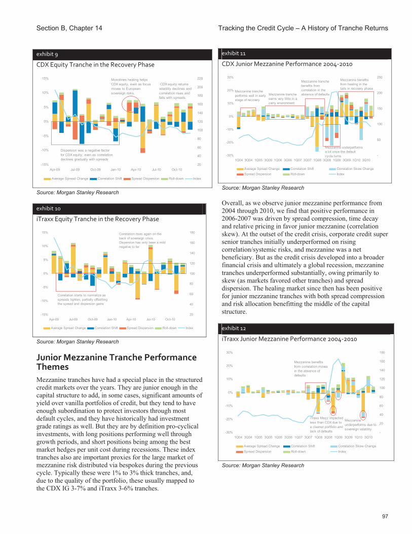
Section B, Chapter 14 Tracking the Credit Cycle – A History of Tranche Returns
97
exhibit 9
CDX Equity Tranche in the Recovery Phase
-15%
-10%
-5%
0%
5%
10%
15%
Apr-09 Jul-09 Oct-09 Jan-10 Apr-10 Jul-10 Oct-1020
40
60
80
100
120
140
160
180
200
220
Average Spread Change Correlation Shift Spread Dispersion Roll-down Index
Dispersion was a negative factor for CDX equity, even as correlation declines gradually with spreads
Monolines healing helps CDX equity, even as focus moves to European sovereign risks.
CDX equity returns volatility declines and correlation rises and falls with spreads.
Source: Morgan Stanley Research
exhibit 10
iTraxx Equity Tranche in the Recovery Phase
-15%
-10%
-5%
0%
5%
10%
15%
Apr-09 Jul-09 Oct-09 Jan-10 Apr-10 Jul-10 Oct-1020
40
60
80
100
120
140
160
180
Average Spread Change Correlation Shift Spread Dispersion Roll-down Index
Correlation rises again on the back of sovereign crisis. Dispersion has only been a mild negative to far
Correlation starts to normalize as spreads tighten, partially offsetting the spread and dispersion gains
Source: Morgan Stanley Research
Junior�Mezzanine Tranche Performance Themes Mezzanine tranches have had a special place in the structured credit markets over the years. They are junior enough in the capital structure to add, in some cases, significant amounts of yield over vanilla portfolios of credit, but they tend to have enough subordination to protect investors through most default cycles, and they have historically had investment grade ratings as well. But they are by definition pro-cyclical investments, with long positions performing well through growth periods, and short positions being among the best market hedges per unit cost during recessions. These index tranches also are important proxies for the large market of mezzanine risk distributed via bespokes during the previous cycle. Typically these were 1% to 3% thick tranches, and, due to the quality of the portfolio, these usually mapped to the CDX IG 3-7% and iTraxx 3-6% tranches.
exhibit 11
CDX Junior Mezzanine Performance 2004-2010
-30%
-20%
-10%
0%
10%
20%
30%
1Q04 3Q04 1Q05 3Q05 1Q06 3Q06 1Q07 3Q07 1Q08 3Q08 1Q09 3Q09 1Q10 3Q10-
50
100
150
200
250
Average Spread Change Correlation Shift Correlation Skew ChangeSpread Dispersion Roll-down Index
Mezzanine tranche earns very little in a carry environment
Mezzanine underperforms a lot once the default cycle turns
Mezzanine benefits from healing in the tails in recovery phase
Mezzanine tranche performs well in early stage of recovery
Mezzanine tranche benefits from correlation in the absence of defaults
Source: Morgan Stanley Research
Overall, as we observe junior mezzanine performance from 2004 through 2010, we find that positive performance in 2006-2007 was driven by spread compression, time decay and relative pricing in favor junior mezzanine (correlation skew). At the outset of the credit crisis, corporate credit super senior tranches initially underperformed on rising correlation/systemic risks, and mezzanine was a net beneficiary. But as the credit crisis developed into a broader financial crisis and ultimately a global recession, mezzanine tranches underperformed substantially, owing primarily to skew (as markets favored other tranches) and spread dispersion. The healing market since then has been positive for junior mezzanine tranches with both spread compression and risk allocation benefitting the middle of the capital structure.
exhibit 12
iTraxx Junior Mezzanine Performance 2004-2010
-30%
-20%
-10%
0%
10%
20%
30%
1Q04 3Q04 1Q05 3Q05 1Q06 3Q06 1Q07 3Q07 1Q08 3Q08 1Q09 3Q09 1Q10 3Q10-
20
40
60
80
100
120
140
160
180
Average Spread Change Correlation Shift Correlation Skew ChangeSpread Dispersion Roll-down Index
iTraxx Mezz impacted less than CDX due to a cleaner portfolio and lack of defaults
Mezzanine benefits from correlation moves in the absence of defaults
Mezzanine underperforms due to sovereign volatility
Source: Morgan Stanley Research

Morgan Stanley Credit Derivatives Insights Handbook
98
Time decay has generally been a positive factor as defaults have been lower than what is implied by single-name spreads. We note that skew and dispersion seem to work together, so when dispersion is rising, investors tend to avoid junior mezzanine risk, and such tranches are driven lower both by market spreads and mezzanine risk aversion. We also note that skew is directional and tends to fall when markets are selling off, which exhibits the beta nature of junior mezzanine tranches. We look below at more detailed performance of junior mezzanine risk per calendar year, highlighting key credit market themes.
exhibit 13
2006: CDX Junior Mezzanine Returns Are Low
-2.5%
-2.0%
-1.5%
-1.0%
-0.5%
0.0%
0.5%
1.0%
1.5%
2.0%
2.5%
Jan-06 Mar-06 May-06 Jul-06 Sep-06 Nov-0630
32
34
36
38
40
42
44
46
48
50
Average Spread Change Correlation Shift Correlation Skew ChangeSpread Dispersion Roll-down Index
Source: Morgan Stanley Research
2006. Credit risk was stable during the year, with bespoke mezzanine issuance driving spreads to extremely tight levels. LBO activity was the primary driver of idiosyncratic risk through the year. Regarding junior mezzanine risk specifically, skew performance was mixed as bespoke mezzanine flows were quite substantial in the market, but not necessarily evenly distributed. Time decay was a steady positive in a zero default environment, and compression was a mild positive, but LBO risk at times hurt mezzanine tranche performance.
2007. The first half of the year was very supportive for corporate credit risk. After the first whispers of trouble from the collapsing Bear Stearns funds, the summer brought the initial contagion from the subprime crisis and along with it, the first significant re-pricings in corporate credit. Much of the returns in junior mezzanine came from time decay and dispersion in the first half of the year. The outperformance owing to skew in the second half of the year was related to correlation rising and strong underperformance of super senior and senior tranches. Dispersion started to be negative in the second half of the year.
exhibit 14
2007: CDX Junior Mezzanine Outperforms Somewhat on Rising Correlation
-10.0%
-8.0%
-6.0%
-4.0%
-2.0%
0.0%
2.0%
4.0%
6.0%
8.0%
Jan-07 Mar-07 May-07 Jul-07 Sep-07 Nov-0730
40
50
60
70
80
90
Average Spread Change Correlation Shift Correlation Skew ChangeSpread Dispersion Roll-down Index
Source: Morgan Stanley Research
2008. Volatility in the credit markets was elevated throughout the year, with the Bear Stearns’ rescue in March serving as an introduction for the extreme events that would ensue in September. Credit spreads reached historic highs in the last several weeks of the year. As credit risk grew more negative, dispersion began to rise, weighing negatively on junior mezzanine performance for most of the year. This was partially offset by skew in the first 8 months of the year; however, even skew turned significantly negative in the risk-off environment following the Lehman bankruptcy. Time decay returns fell significantly, rising only in December.
exhibit 15
2008: CDX Junior Mezzanine Underperforms Substantially on Dispersion and Skew Changes
-30%
-20%
-10%
0%
10%
20%
30%
Jan-08 Mar-08 May-08 Jul-08 Sep-08 Nov-0850
100
150
200
250
300
Average Spread Change Correlation Shift Correlation Skew ChangeSpread Dispersion Roll-down Index
Source: Morgan Stanley Research

Section B, Chapter 14 Tracking the Credit Cycle – A History of Tranche Returns
99
2009. The market got off to a weak start in the first quarter, but many dislocated relationships healed. Credit had a strong rally in the remainder of the year, with more dislocation healing, and most new risk taking was in corporate bonds rather than CDS, healing the basis. Skew was a strong positive for junior mezzanine for most of the year as 2008 dislocations began to heal, causing mezzanine to outperform. Dispersion was high early in the year as default levels remained elevated, but as recovery gained momentum and defaults fell, spread compression generated positive performance for junior mezzanine. Time decay was positive throughout the year.
exhibit 16
2009: CDX Junior Mezzanine Heals Eventually with Spread Compression Aiding
-15%
-10%
-5%
0%
5%
10%
15%
Jan-09 Mar-09 May-09 Jul-09 Sep-09 Nov-0950
100
150
200
250
Average Spread Change Correlation Shift Correlation Skew ChangeSpread Dispersion Roll-down Index
Source: Morgan Stanley Research
2010. Credit markets rallied early in the year, which was ultimately tempered by significant European sovereign volatility in May/June. The summer brought on a slow healing, followed by a strong year-end rally. Spread compression was a positive for junior mezzanine performance throughout the year. Skew was driven by a risk-on / risk-off environment given huge moves in underlying spreads. Time decay was a solid positive through the year as default risk was low.
exhibit 17
2010: CDX Junior Mezzanine Performs Well Outside of Sovereign Crisis on Compression and Skew
-20%
-15%
-10%
-5%
0%
5%
10%
15%
Jan-10 Mar-10 May-10 Jul-10 Sep-10 Nov-1050
75
100
125
150
Average Spread Change Correlation Shift Correlation Skew ChangeSpread Dispersion Roll-down Index
Source: Morgan Stanley Research
Senior Mezzanine Tranche Performance Themes Senior mezzanine tranches during much of the last credit cycle were considered “orphaned” credit risk. Too senior to generate enough yield for those with strong appetites, yet too junior for those investors who required extremely remote risk, these tranches (CDX IG 7-10% and iTraxx 6-9%) were often an afterthought, at least until the credit crisis drove risk allocations up the capital structure and ratings models and increased defaults served to differentiate them from their senior tranche brethren. In this section we examine the ways this more subordinated yet still “mezzanine” risk behaved throughout the cycle.
exhibit 18
CDX Senior Mezzanine Performance 2004-2010
-20%
-15%
-10%
-5%
0%
5%
10%
15%
20%
1Q04 3Q04 1Q05 3Q05 1Q06 3Q06 1Q07 3Q07 1Q08 3Q08 1Q09 3Q09 1Q10 3Q10-
50
100
150
200
250
Average Spread Change Correlation Shift Correlation Skew ChangeSpread Dispersion Roll-down Index
Mezzanine underperforms a lot once the default cycle turns
Senior mezz benefits in Auto Crisis
Mezzanine benefits from dispersion in recovery phase
Mezzanine tranche performs well in early stage of recovery
Tight spreads, low return environment for senior mezzanine
Source: Morgan Stanley Research

Morgan Stanley Credit Derivatives Insights Handbook
100
2006. This was a rather uneventful year for senior mezzanine risk, as market flows and attention were dedicated to the enormous wave of bespoke flows which had an outsized impact on the tranches just below senior mezzanine. Time decay provided a steady, if small, positive performance, while dispersion was flat for the entire year. Skew was positive at the beginning of the year, with a brief, small negative period in the third quarter, ending the year relatively flat.
exhibit 19
2006: CDX Senior Mezzanine Largely Uneventful
-0.6%
-0.4%
-0.2%
0.0%
0.2%
0.4%
0.6%
Jan-06 Mar-06 May-06 Jul-06 Sep-06 Nov-0630
35
40
45
50
Average Spread Change Correlation Shift Correlation Skew ChangeSpread Dispersion Roll-down Index
Source: Morgan Stanley Research
2007. While the bottom of the capital structure was digesting the first hints of the impending crisis, senior mezzanine risk performance began to get more interesting. Time decay picked up steadily throughout the year, while dispersion began to factor into tranche performance, though still small. Skew was overall flat the first half of the year, and became a much bigger contributor to positive returns over the summer given the underperformance of more senior tranches.
exhibit 20
2007: CDX Senior Mezzanine Benefits from Super Senior Issues, But Turns Weaker Later
-4%
-3%
-2%
-1%
0%
1%
2%
3%
Jan-07 Mar-07 May-07 Jul-07 Sep-07 Nov-0730
40
50
60
70
80
90
Average Spread Change Correlation Shift Correlation Skew ChangeSpread Dispersion Roll-down Index
Source: Morgan Stanley Research
2008. The impact of rolldown (time decay) became more pronounced as the expected loss on the underlying index rose substantially, up through 3-7% and into the senior mezzanine tranche, substantially changing the fundamental nature of this risk. Whereas before this tranche tended to behave more like its more senior relatives, elevated overall credit risk made this now solid mezzanine risk. Dispersion started to have a positive impact in the second quarter and really drove performance during the peak of the crisis. Skew, however, had increasingly negative momentum and more than offset any gains made by dispersion and time decay.
exhibit 21
2008: CDX Senior Mezzanine Suffers with Other Mezzanine Risk
-20%
-15%
-10%
-5%
0%
5%
10%
15%
20%
Jan-08 Mar-08 May-08 Jul-08 Sep-08 Nov-0850
100
150
200
250
300
Average Spread Change Correlation Shift Correlation Skew ChangeSpread Dispersion Roll-down Index
Source: Morgan Stanley Research
2009. The market got off to a weak start, but credit had a strong rally in the back half of the year. In senior mezzanine risk, rolldown generated positive performance, peaking in the first quarter of 2009 and remaining elevated throughout the rest of the year. Performance due to dispersion was volatile; in the beginning of the year it contributed negatively, like the junior mezzanine tranches, but soon turned positive in the spring as spreads came down slightly, and remained positive for the rest of the year. Skew remained negative, though to a lesser degree than 2008.
2010. As credit markets continued to heal, time decay remained a major positive factor in senior mezzanine risk. In the first quarter, this was offset by spread dispersion, though between spring and fall spread dispersion was a positive contributor to returns. Skew performance was mixed and somewhat volatile, ending the year flat.

Section B, Chapter 14 Tracking the Credit Cycle – A History of Tranche Returns
101
exhibit 22
2009: CDX Senior Mezzanine Recovers More Quickly than Other Mezzanine
-15%
-10%
-5%
0%
5%
10%
15%
Jan-09 Mar-09 May-09 Jul-09 Sep-09 Nov-0950
100
150
200
250
Average Spread Change Correlation Shift Correlation Skew ChangeSpread Dispersion Roll-down Index
Source: Morgan Stanley Research
exhibit 23
2010: CDX Senior Mezzanine More Mixed with Sovereign Volatility
-10%
-8%
-6%
-4%
-2%
0%
2%
4%
6%
8%
10%
Jan-10 Mar-10 May-10 Jul-10 Sep-10 Nov-1050
75
100
125
150
Average Spread Change Correlation Shift Correlation Skew ChangeSpread Dispersion Roll-down Index
Source: Morgan Stanley Research
Senior Tranche Performance Themes As equity and junior mezzanine tranches jostled for the spotlight in the 2005, super senior tranches with spreads in the teens that rarely moved were the less interesting part of the market, until the advent of levered super senior (LSS) flows. In an environment where central banks were considered to have mastered the control of tail scenarios, super senior was considered dead money and any level of super senior spread would be considered worth selling into. LSS flow pushed super senior spreads into single digits. The combination of the extremely low volatility environment, high leverage, long duration, the presence of unwind triggers (both spread and ratings driven), and in hindsight, poor entry points proved to be the undoing of super senior structures.
Many of these structures were being unwound quite early in the crisis (late 2007 and early 2008).
exhibit 24
Super Senior vs Index Spread (iTraxx)
0
50
100
150
200
250
Jul-0
6
Oct
-06
Jan-
07
Apr
-07
Jul-0
7
Oct
-07
Jan-
08
Apr
-08
Jul-0
8
Oct
-08
Jan-
09
Apr
-09
Jul-0
9
Oct
-09
Jan-
10
Apr
-10
0
20
40
60
80
100
Index (LHS) 22-100% (RHS)
Era of single digit super senior spreads. Low volatility encourages 10x leveraged SS, initially 5yr but later to 7yr and 10yr
LSS unwinds on spread and ratings triggers, Monoline fears. No corporate defaults yet
Systemic crisis, monoline/Insurer fears. No Corporate defaults yet.
Index spikes to wides even as super senior starts healing. Financial defaults cause loss of subordination and hurt Junior Mezzanine. Crisis has moved from systemic to cyclical.
Super senior has outperformed the capital structure recently but remains wide by pre-crisis standards.
Source: Morgan Stanley Research
Junior super senior risk, represented by the 15-30% tranche in CDX IG and the 12-22% in iTraxx, has been a relatively less active part of the tranche market, with pricing primarily driven by equity and mezzanine below and levered super senior flows above. A key difference in analyzing the importance of underlying factors in driving tranche performance for senior risk is that with their lower deltas and subordination, roll-down has a smaller role to play relative to the higher delta junior tranches. Relative to the index, (delta-adjusted), these tranches have a “negative” roll-down.
2H07 – 1H08. Unlike equity or mezzanine, the impact of correlation (parallel or skew) is not as straightforward to analyze. In general we have found that correlation moves tend to have a largely directional impact for junior tranches, i.e., large moves wider in spreads tend to be accompanied by a move higher in correlation for equity (lower in skew for mezzanine), which then has an offsetting effect for equity and exacerbates the impact of spreads for mezzanine.
In Exhibit 25 we show that correlation skew is a cyclical indicator rather than just a reflection of spread directionality for the more senior tranches. Through the summer of 2007 and early 2008, senior tranches underperformed junior tranches as developing subprime concerns sparked fears of a credit crisis. This period also witnessed leveraged super senior unwinds driven by spread and rating fears. Through this period, risk flowed into senior tranches, which can be seen by the significant negative contribution provided by the skew component.

Morgan Stanley Credit Derivatives Insights Handbook
102
exhibit 25
2007: Senior Underperforms in the Rising Systemic Risk Environment
-1.0%
-0.8%
-0.6%
-0.4%
-0.2%
0.0%
0.2%
0.4%
0.6%
0.8%
Jan-07 Mar-07 May-07 Jul-07 Sep-07 Nov-0730
40
50
60
70
80
90
Average Spread Change Correlation Shift Correlation Skew ChangeSpread Dispersion Roll-down Index
Source: Morgan Stanley Research
2H08. As the credit crisis morphed into a full-blown economic recession accompanied by significant corporate defaults, senior risk outperformed equity and mezzanine risk through the second half of 2008. A combination of policy action aimed at reducing systemic stresses and idiosyncratic default concerns on the back of defaults in the IG index led to risk flowing down the capital structure. Exhibit 26 captures the positive impact of moves in correlation skew for the 15-30% tranche even as spreads continued to widen through the second half of 2008. This was in stark contrast to the market moves seen from July 2007 – May 2008, when spread changes and correlation skew both contributed negatively to tranche performance.
exhibit 26
2008: Senior Underperforms Early on Systemic Risk, but Outperforms During the Recession
-8%
-6%
-4%
-2%
0%
2%
4%
6%
Jan-08 Mar-08 May-08 Jul-08 Sep-08 Nov-0850
100
150
200
250
300
Average Spread Change Correlation Shift Correlation Skew ChangeSpread Dispersion Roll-down Index
Source: Morgan Stanley Research
2009. Dispersion played a more significant role in senior tranche performance in early 2009. Even as credit spreads
started tightening from elevated levels, tails risks persisted (largely in the form of distressed financials), as did defaults, which meant that idiosyncratic risk still existed. This dispersion worked favorably for senior risk, which was now increasingly OTM from a default breakeven perspective, because fat portfolio tail risks were being disproportionately allocated to the junior tranches. This trend subsided towards the end of the year as the economic backdrop improved and defaults started subsiding.
2010. Spread compression occurred at a portfolio level in 2010 and as such tail names tightened significantly, leading to outperformance of junior tranches. Exhibit 28 shows the negative impact that spread dispersion had on 15-30% performance through most of the year.
exhibit 27
2009: Senior Benefits from Dispersion
-4%
-3%
-2%
-1%
0%
1%
2%
3%
4%
Jan-09 Mar-09 May-09 Jul-09 Sep-09 Nov-0950
100
150
200
250
Average Spread Change Correlation Shift Correlation Skew ChangeSpread Dispersion Roll-down Index
Source: Morgan Stanley Research
exhibit 28
2010: Senior Underperforms on Sovereign Risks and Improving Credit Quality
-2.0%
-1.5%
-1.0%
-0.5%
0.0%
0.5%
1.0%
1.5%
Jan-10 Mar-10 May-10 Jul-10 Sep-10 Nov-1050
75
100
125
150
Average Spread Change Correlation Shift Correlation Skew ChangeSpread Dispersion Roll-down Index
Source: Morgan Stanley Research

Section C
Credit Portfolio Management

Morgan Stanley Credit Derivatives Insights Handbook
104
Chapter 15
Bank Loan Hedging Today – CPM Part I May 30, 2008
Sivan Mahadevan Vishwanath Tirupattur Ashley Musfeldt Andrew Sheets Phanikiran Naraparaju
As much as credit derivatives flows over the past year have been dominated by a wide range of institutions trading, hedging and speculating on credit risk, bank loan hedgers are both the market’s original and natural buyers of protection. Corporate CDS contracts were designed for this community more so than any other, and many of the nuances investors deal with in CDS contracts relate to the idiosyncrasies of loan risk that is on the books of banks.
Credit portfolio management (CPM) is the industry term used to describe the practice of managing credit exposures in corporate lending institutions, mainly large banks but also the lending businesses within dealers and insurance institutions to some degree. Every major bank lending institution has a significant effort devoted to it. While this is not a new art by any means, CPM practitioners face both a very interesting and challenging environment going forward, a function of the current credit environment, a significant repricing in corporate and structured credit, market liquidity issues and the secular regulatory changes related to the transition from Basel I to II, accounting shifts and general local jurisdiction oversight.
For those within the CPM world, there is a lot to consider, and in this chapter we attempt to outline ten themes to set the stage for further research and strategies. For the majority of market participants who will watch CPM activity from the sidelines, it is difficult to say whether the resulting credit flows are bullish or bearish, but structurally speaking, as banks move from a Basel I to Basel II framework, economic capital and regulatory capital will become more closely aligned. For many banking institutions, full implementation of Basel II is only 18 months away, with parallel processing going on now, and some amount of Basel II implementation starting at the beginning of 2009.
WHY IS CPM IMPORTANT? For many, bank loan hedging vernacular is a foreign tongue. For those who are willing to learn a bit (and we encourage it), we recommend a few resources. Credit exposure management by banks and other financial institutions involves both long and short credit investments, employs credit derivatives technology, and creates flows that are driven both by economic and regulatory capital needs. The International Association for Credit Portfolio Managers (IACPM) is a professional organization that brings CPM practitioners together globally to address issues and
opportunities. There are currently 88 financial institutions that are members of the IACPM, from 16 countries (for a general description of CPM activities and links to many of the relevant public documents, see www.iacpm.org).
exhibit�1�
Capital�Requirements:�Basel�I vs. Basel II
0%
1%
10%
100%
AAA Aa3 A3 Baa3 Ba3 B3 Caa3
Tranche Rating
Reg
ulat
ory
Cap
ital
Basel I
Basel II (Base)
Basel II (Senior-most)
Source: Morgan Stanley
A lot of CPM work involves interpreting Basel I and Basel II regulatory capital regimes, and mixing it with local jurisdiction regulatory environments, accounting practices and other factors to create efficient exposures to retained credit risk while meeting economic capital goals.
CHALLENGES FACING BANK LOAN HEDGERS We have spent a considerable amount of time recently with the CPM community, both to understand their challenges and to discuss strategies for resolving them. In this market and regulatory environment, the CPM community faces many challenges and has a lot of work to do. The good news is that economic and regulatory capital will be more closely aligned when they are done, and this will make the financial system more sound, as at least some of the problems of this systemic crisis can be blamed on disconnected regulatory and economic capital regimes. We list and briefly describe below some of the challenges and potential solutions for a number of topics that we believe are relevant, and caution that the list is by no means all-encompassing.
1. BASEL I TO BASEL II TRANSITION Perhaps Basel I/II regulatory capital regimes are the most commonly associated term with CPM, and a lot of what banks need to do over the next several quarters is related the transition from Basel I and II.

Section C, Chapter 15 Bank Loan Hedging Today – CPM Part I
105
In simple terms, one of the big differences between Basel I and II is the regulatory capital treatment for retained credit risk. Owning the junior portion of credit risk versus owning only the senior exposure of credit risk in many cases is not treated differently under Basel I, so bank loan hedgers can efficiently gain regulatory capital relief by buying protection on senior parts of a portfolio (i.e., 3-100%), because senior parts trade at tighter spreads. One does not have to be a market expert to realize that such a regulatory capital approach stands in contrast to economic capital, where junior tranches have more MTM and default risk than senior tranches, for a given notional amount.
Under Basel II, the risk weightings are high for junior tranches and fall off dramatically as one goes up the capital structure, which is very much in line with economic capital, in our view (see Exhibit 1). This is also true for low rated assets compared to highly rated assets. We offer the caveat that local jurisdictions can treat risk rated below investment grade differently (full deduction in some cases for BB- and below), but the general theme is consistent. For investment grade portfolios, it is possible to release more capital at the portfolio level simply by transitioning from Basel I to Basel II – risk weights move to 50% to 75% for BBB portfolio depending on the approach used relative to a 100% under Basel I. The implication is that, generally speaking, holding securitized risk of investment credit portfolios is more attractive under Basel II, although there are important implications based on the tranche rating itself (see Exhibit 2).
exhibit 2
Retained Credit Efficiency Shifts Radically from Basel I to II
0%
100%
200%
300%
400%
500%
600%
0% 5% 10% 15%Tranche Attachment Point
Cur
rent
Spr
ead/
Reg
ulat
ory
Cap
ital
5% thick tranche (Basel I)
5% thick tranche (Basel II)
Sweet Spot From LongPerspective Under Basel II
0%
20%
40%
60%
80%
100%
120%
0% 5% 10% 15%Tranche Attachment Point
Cur
rent
Spr
ead/
Reg
ulat
ory
Cap
ital
x-100% (Basel I)
x-100% (Basel II)
Sweet Spot From LongPerspective Under Basel II
Source: Morgan Stanley
For below investment grade portfolios, the outcome is a bit more complex – depending on the assumptions/approach, the risk weight for such portfolios could be higher under Basel II, although the higher quality securitized tranche benefits under Basel II. This actually creates opportunities for significant differentiation in capital management in the below investment grade space – partially hedging a loan portfolio has a lot of scope under Basel II. We provide a flavor of impact on investment grade securitized risk here and will follow up in detail on the impact on both investment grade and below investment grade securitizations.
In Exhibit 2, we show the efficiency of retaining certain parts of credit risk in a portfolio of corporate credit with a similar ratings and risk profile to the 5-year CDX IG (tranche attachment vs. the spread of this risk divided by the product of risk weights and an 8% capital regime). The top chart illustrates that the sweet spot for retained credit risk moves from a very junior attachment under Basel I to a more senior attachment (say around 4% or 5%) under Basel II. This

Morgan Stanley Credit Derivatives Insights Handbook
106
example assumes tranches that are 5% thick. Very junior tranches have the most to lose under Basel II.
However, since many bank loan hedgers are used to thinking about X-100% hedges given their efficiency under Basel I, in the second chart in Exhibit 2, we show the poor efficiency of such hedges under Basel II (or said differently, they actually can look attractive from a long perspective today given the market repricing).
As a caveat, we note that this is a very simplified example, and the details of any portfolio and hedging scheme can result in different outcomes, although we expect the general themes to be consistent with this analysis.
One of the key challenges for CPM practitioners today is efficiently moving from Basel I type hedges to Basel II. In our simple view of the world, the two capital regimes stand in stark contrast to one another, and as such there is no “magic” way of hedging efficiently under both regimes, although there are partial solutions that, in our view, would involve owning protection on tranches with junior mezzanine type attachment points.
2. DYNAMIC MANAGEMENT UNDER BASEL II One of the key benefits to operating under a Basel II world, in our view, is that there is scope for dynamically managing portfolio hedges, as market pricing changes. Given the non-constant nature of risk weightings for retained risk, CPM practitioners will have an opportunity to make adjustments to their hedges based on market movements in structured credit pricing, single-name dispersion, etc.
The flat risk weight structure under Basel I implies that ratings migration of the underlying portfolio has little impact. Even cataclysmic shifts in pricing across the structured credit capital structure like the one we recently went through do not alter the hedging framework much – even though economically the risk environment has changed dramatically. Stability of regulatory capital strategies under Basel II is a function of both pricing and ratings. Under Basel II, given the repricing from last year, senior mezzanine risk is significantly more attractive today – and while X-100% hedges with low attachments might have made sense in 2007, there is more incentive to be long senior mezzanine type of risk today rather than using it in a hedge (see Exhibit 3). On the other hand negative ratings migrations in today’s environment will compel investors to add subordination to make it regulatory capital efficient under Basel II – consistent with economic logic.
exhibit 3
Basel II Retained Credit Risk – Repricing Matters
0%
100%
200%
300%
400%
500%
600%
0% 5% 10% 15%Tranche Attachment Point
Spr
ead/
Reg
ulat
ory
Cap
ital
5% thick tranche 1yr back (Basel II)
5% thick tranche (Basel II)
x-100% 1yr back (Basel II)
x-100% (Basel II)
Source: Morgan Stanley
3. LOAN OPTIONALITY Most bank loans have variable maturities, potentially variable coupons, and even their utilization can vary (i.e., untapped or partially tapped revolvers). Simply put, loan portfolios have short convexity exposures, given the options that the lenders have sold to the issuers. While the pricing of the loan instruments might compensate banks for some amount of negative convexity, in general most CPM specialists need other tools to hedge convexity exposure.
As credit investors have begun to dominate the momentum of credit derivatives markets over the past many years, CDS contracts have been trending toward bullet type contracts as most investors prefer simple fixed maturity credit risk. Restructuring is not a standard credit event in some forms of LCDS today, and while non-standard CDS is always a possibility, the illiquidity of such instruments is generally an issue.
In the mortgage world, hedgers tend to use swaptions as a way to hedge the negative convexity exposure of being short prepayment options. In many ways, their problems are analogous to bank loan hedgers, and we would argue that credit option instruments might present an interesting solution to convexity issues. Index options are a natural solution to hedge overall portfolio convexity, and we expect activity to increase here. There are solutions at the single-name level that will be necessary as well, either through cancellable forms of CDS/LCDS contracts (more likely) or options on single-names (less likely).
4. ILLIQUID CREDITS Many CPM specialists we meet cite illiquid credits as being a top challenge for hedging. Illiquidity can have many faces too, including both smaller companies (from a debt market capitalization perspective) and loans that are linked to (or secured by) hard to value assets, cashflow streams and the

Section C, Chapter 15 Bank Loan Hedging Today – CPM Part I
107
like. There is no single solution to this problem, but perhaps some creative ones. The growth of loan indices (LevX and LCDX) is certainly improving liquidity for quite a number of secured credits in both the US and Europe, and such recent liquidity boosts might help CPM practitioners in this regard. There are also overlay strategies including the indices themselves or credit proxies. But for more illiquid direct exposures, in this market environment, the dealer community is unlikely to want to take on highly illiquid credit risks, so any transfer of such credit risks by CPM specialists will likely need to involve linking the credit risk to a product that could be offered to an end investor, or employing hedges on the real assets (e.g., commodities) being referenced by the credit, or both.
5. LIQUIDITY/FUNDING Liquidity risk from a funding perspective (i.e., using short-term funding to finance the purchase of long-term assets in SIV-like structures) was one of the most painful lessons learned in this credit cycle, both for those who lent and borrowed in this framework. Liquidity and funding costs have driven performance of AAA assets and the CDS-bond basis, among other relationships. Funding has also affected product securitization strategies. Banks might also consider more efficient mechanisms for funding, given the current state of their balance sheets, and some of the options might include securitizing credit risk into CDOs whose senior tranches can be posted to the Fed/ECB as collateral, or using more elaborate CPPI type structures to create funding efficiencies.
6. COUNTERPARTY RISK Clearly a topic with a lot of market focus today, counterparty risks on CDS trades (long or short) are a key focus point for CPM practitioners. It is certainly good news that Basel II considers the impact of counterparty risk in its accord, but the approach might be overly simple. There are generally two methods to account for counterparty risk, the substitution approach and the double-default approach. Double-default provisions are meant to reduce risk weights cognizant of the lower probability of joint default of the exposure and protection bought. However, double-default provisions are not applicable to multiple name credit derivatives or index-based products, synthetic securitization – so substitution is the fallback.
Under substitution, protection purchased on a credit will only reduce risk weightings on the credit to the level of the protection provider (i.e., buying protection on a BBB credit from a AA entity would result in a net risk weighting of AA). Selling protection on a single tranche say 5-7% results in different capital requirement from selling protection on the index and buying protection on 0-5% and 7-100% parts of the capital structure due to the difference in the way counterparty exposures are accounted. For example, 5-100% protection purchased against 0-100% exposure (rated Baa1) would result in a capital requirement of $6.02MM, which is
higher (because of counterparty charges) than from simply being long $5MM of 0-5% (rated B2) which requires a full deduction, i.e., capital of $5MM.
But there is one potential problem here. The vast majority of CDS trades today are fully collateralized to their market value, with certain thresholds for daily moves depending on the quality of the counterparty. This effectively reduces counterparty risk in the system to the “gap risk” of not having enough collateral (see “Stress Testing the CDS Market,” January 18, 2008). We do not believe that the Basel II Accord addresses this collateral posting, which is a shortcoming in our view.
7. RATINGS One of the criticisms of Basel II is its reliance on ratings within structured forms of credit including securitizations (for the rest, banks will rely on internal credit assessments). Ratings are clearly an issue today with the credibility of rating agencies being questioned in the market. Generally, when a public rating is available, banks must use them under the standard or RBA approaches to calculate risk weightings on retained credit risk. The supervisory formula is available when public ratings are not available, and the calculation is similar in scope to rating agency models in that subordination, tranche thickness, number of credits in the pool, and loss given default of the underlying portfolio is taken into consideration.
Nevertheless, there is a general reliance on ratings under Basel II for structured credit risk, and as such the Financial Stability Forum (FSF) is addressing rating agency operating issues including the quality of the ratings process, potential conflicts of interest, more information on risk characteristics, data quality, due diligence by ratings users, and the role of ratings by regulators1. We do not see a lot of direct changes to ratings of retained corporate credit risk as a result of the FSF efforts, except for re-securitizations like CDO-squared transactions. The ratings process might be better vetted as a result of FSF, but whether or not it is successful, we believe that bank regulatory capital will continue to be heavily dependant on external ratings.
8. FAIR VALUE OPTION, ACCOUNTING, CASH VS. CDS Among the most complicated aspects of the CPM world is related to accounting, especially in the world of fair value. Separation of risks from the banking and trading books is a central issue, and the differing accounting treatment of cash assets and synthetic hedges continues to be problematic for many banking institutions from an income statement perspective. It has been common in the past and will likely be in the future to add in macro forms of long credit exposure
1 See Report of the Financial Stability Forum on Enhancing Market and Institutional Resilience, April 7, 2008.

Morgan Stanley Credit Derivatives Insights Handbook
108
(without much idiosyncratic exposure) to trading books offset MTM volatility of credit hedges.
9. MODEL RISK The systemic nature of the current credit crisis was atypical in the sense that there is a disconnect between mark-to-market losses and investor perception of the real losses (outside the obvious troubled sectors). This disconnect is so extreme as to force rethinking of models including correlation calculations, recovery modeling and the like. While events of such magnitude may not be an annual
occurrence, it has stirred up a debate on fair value accounting and the use of models with and without market inputs.
10. INSURANCE COMPANY ISSUES While much of the focus in CPM is related to banks and their corporate credit assets, insurance companies practice CPM as well, and Solvency II is the set of regulatory requirements that apply to European insurance companies. Similar in theme to Basel II, Solvency II will move regulatory and economic capital closer together.

109
Chapter 16
Basel II Based Hedging – CPM Part II June 13, 2008
Sivan Mahadevan Phanikiran Naraparaju Vishwanath Tirupattur Ashley Musfeldt Andrew Sheets
We continue with our focus on the secular changes that are afoot in the bank loan hedging community, the market’s natural and original buyers of protection. In Chapter 15, we described the landscape today and the challenges and opportunities facing credit portfolio managers (or CPM, the industry term used for bank loan hedging). In this chapter, we focus on a specific theme, namely capital efficiency under Basel II for those institutions that use tranched portfolio protection programs as a means of hedging (which is quite common). The market implications of these hedging programs are quite significant in our view.
Under the Basel I regime, much investment grade rated credit risk is treated equally, and as such, banks who operate under Basel I have not had much motivation to either invest directly or indirectly (through retained credit risk after hedges) in senior forms of credit risk, given their lower yields. In fact, one could argue that the steady trend of the WACC curve moving to the lower rungs of the investment grade world has something to do with the lack of motivation among banks (under Basel I) to finance high quality corporations.
Under Basel I, from the perspective of a bank with exposure to investment grade rated loans and revolvers, deciding which part of the portfolio to retain becomes more a function of spread rather than expected losses, ratings, default-risk remoteness, seniority and the like. This is one of the reasons why buying 3-100% protection (i.e., banks retaining the 0-3% part of the loan portfolio) has been a reasonably good Basel I strategy, given the much lower cost. But as we discussed in Chapter 15, under Basel II, we move to a regime where economic and regulatory capital become more closely aligned, and as such, what is efficient to retain is a function of risk remoteness, expected losses and market prices.
We focus this chapter on assessing the efficiency of retained credit risk for portfolios of investment grade loan exposure under Basel II, using a host of tranched portfolio hedging alternatives. Details and assumptions clearly matter, and we caution that our approach should be considered a general one. We also note that investment grade portfolios benefit from regulatory capital relief simply by moving from Basel I to Basel II, and that a repriced credit and structured credit market will alter portfolio efficiency quite significantly as well.
exhibit 1
Sample of Basel II Efficient Solutions CDX 5yr Bespoke CDX 10yrPortfolio Spread (%) 1.1% 1.7% 1.1%Portfolio Rating Baa2 Baa1 Baa2Spread per unit of RC 26% 40% 27% Efficient Solutions and SRC (Spread per unit Reg
Capital) Type CDX 5yr Bespoke CDX 10yrTwo Tranche Retain 2.5-100%
(SRC 115%) Retain 2-100%
(SRC 192%)Retain 3.5-100%
(SRC 117%)Two Tranche Retain 4-100%
(SRC 110%) Retain 3-100%
(SRC 189%)Retain 4.5-100%
(SRC 108%)Three Tranche Retain 0%-0.5%
and 2.5%-100% (SRC 109%)
Retain 0%-0.5% and 1.5%-100%
(SRC 173%)
Retain 0%-0.5% and 3.5%-100%
(SRC 105%)Four Tranche Retain 3%-9%
and 10%-100% (SRC 108%)
Retain 2.5%-7%and 8.5%-100%
(SRC 190%)
Retain 4.5%-10%and 11%-100%
(SRC 109%) Source: Morgan Stanley
exhibit 2
Tranching Alternatives and Nomenclature
Long Index
5-100% tranche risk retained
Equity tranche (0-5%) hedged
9-100% tranche risk hedged
Equity tranche (0-5%) hedged
5-9% retained
9-12% hedged
Equity tranche (0-5%) hedged
12-100% tranche risk retained
5-9% retained
2T – H-L
3T – H-L-H
4T – H-L-H-L
Sell Protection on 5-100% tranche risk
Equity tranche (0-5%) No position
2T – N-L
Source: Morgan Stanley
OUR METHODOLOGY Basel II does not provide a framework for regulatory capital relief from a hedging perspective specifically. Instead, for the analysis included in this chapter, we focus on a bank’s long credit exposure, net of hedges (and the associated counterparty costs of those hedges), using the following framework:
� We assume that a bank is long the credit risk of a loan portfolio and considers tranche protection as a way of isolating and selling off the “expensive” parts of this risk (from a capital perspective) so that this bank can retain the more efficient parts of the credit risk of the portfolio.
� We assume two portfolios, one mirroring CDX and the other a global bespoke portfolio that represents a wider

Morgan Stanley Credit Derivatives Insights Handbook
110
spread universe of investment grade names, but marginally higher in quality with more sector concentration. Clearly, results are very dependent on the actual portfolios, and any specific solution may differ materially from what we present here. Solutions involving non-investment grade portfolios will be considerably different.
� We calculate the return on capital by translating the retained credit risk into a rating(s), using the Moody’s synthetic CDO rating approach for corporate credit, which is closest to Basel II’s internal approach, given the focus on expected losses instead of first dollar losses (the latter being the S&P approach).
� We note that banks may use their internal frameworks or the ratings of any agency, so our approach may not exactly match the approach of any one CPM practitioner, but we believe it is generally useful.
� There is a counterparty-related regulatory capital cost for hedging credit risk, based on the actual counterparty rating (internal or external). We assume a counterparty rating of A1 and assume the substitution approach attracts a capital of 1.2%.
� There are an infinite number of ways that a portfolio of loans could be sliced into tranches. For simplicity’s sake, we limit our approach to solutions that incorporate two, three and four tranches and make thickness assumptions as well (see Exhibit 2 for the nomenclature we use).
� For each tranche, we estimate an implied rating using the Moody’s approach, and we also imply tranche pricing from CDX/iTraxx and bespoke correlation surfaces.
� We calculate spread on capital as the spread earned on the notional amount, divided by the product of the risk weight of the retained credit risk and 8% (representing our assumption for the amount of capital a bank will hold for a non-deducted asset). We subtract the regulatory capital charge for hedging.
� This approach is very simple, and we fully realize that any one bank’s approach can be an evolving process given that interpretation of guidelines is still not certain across different jurisdictions.
� The minimum amount of risk transfer and type of risk transfer required to be eligible for regulatory capital relief also varies across different jurisdictions.
exhibit 3
Two Tranches – X-100% Attractive to Retain Today
0%
20%
40%
60%
80%
100%
120%
140%
0% 2% 4% 6% 8% 10% 12% 14% 16% 18% 20%
Equity Tranche Detachment (2-Tranche Solution)
Spr
ead/
Reg
ulat
ory
Cap
ital 2T-L-H
2T-H-LIndex
Source: Morgan Stanley
exhibit 4
Two Tranches – Closer Call a Year Ago
0%
2%
4%
6%
8%
10%
12%
14%
16%
0% 2% 4% 6% 8% 10% 12% 14% 16% 18% 20%
Equity Tranche Detachment (2-Tranche Solution)
Spr
ead/
Reg
ulat
ory
Cap
ital
2T-L-H2T-H-LIndex
Source: Morgan Stanley
TWO-TRANCHE SOLUTIONS In Exhibit 3, we show the results of a two tranche solution for the 5-year CDX index, graphing the spread/required capital (which is a measure of return on capital) on the Y-axis. On the x-axis we graph various detachment points between the equity tranche and senior tranche. The flat line represents the return on capital for simply holding the CDX portfolio with no hedges, so it is the return-on-capital bogey to beat. The two curves in the graph represent: a) retaining the equity tranche and hedging with the senior tranche (the lower curve), and b) retaining the senior tranche and hedging with the equity tranche (the higher curve). We make a few observations.
� In general, retaining the senior risk and hedging the equity risk is far more efficient than the other way around, with the optimal points of efficiency achieved by retaining tranches between 2-100% to 5-100%.

Section C, Chapter 16 Basel II Based Hedging – CPM Part II
111
� The same analysis using market pricing from one year ago shows quite a different picture. Retained equity solutions could have competed reasonably well with retained X-100% solutions a year ago even under Basel II assumptions, given the very tight pricing of senior and super senior risk. Today retained equity solutions are considerably poorer value (see Exhibit 4).
� Today any retained X-100% type strategy attaching anywhere up to 20% is more efficient than plain vanilla portfolio exposure.
� The moral of course is that big shifts in pricing can alter the efficiency of specific solutions, and strategies are likely to be more dynamic under Basel II.
THREE-TRANCHE SOLUTIONS The world does not necessarily have to be limited to 2-tranche solutions, so we extend the analysis to three tranches, and hence show a 3-dimensional graph (Exhibit 5, where the Z-axis is the detachment of the equity tranche, and the X-axis is the detachment of the middle mezzanine tranche). We add two more solution types: a) Hedging mezzanine risk and retaining equity and super senior risk; b) hedging equity and super senior risk while retaining mezzanine risk.
� Retaining senior mezzanine risk (say 3-9%) is among the most efficient of the pure three-tranche solutions.
� Retaining thin equity tranches plus super senior tranches that include senior mezzanine risk is also efficient (i.e., buying 1-2% protection and retaining 2-100% and 0-1% risk).
� At higher attachments, say greater than 3%, retaining 3-10% risk is more efficient than retaining 0-3% and 10-100% risk. Overall, retaining senior mezzanine still provides the most stable solution, in our opinion.
� However, two-tranche X-100% strategies outperform either of the three-tranche strategies described above, as the cost of buying super senior protection is high.
exhibit 5
Three Tranches – Senior Mezz Attractive to Retain
1% 3% 4% 6% 7% 9% 10% 12% 13% 15% 16% 18% 19%
1%
4%
6%0%
5%
10%
15%
20%
25%
30%
35%
40%
45%
Mezzanine Tranche Detachment
Equi
ty
Tran
che
Det
achm
ent
1.00%1.50%2.00%2.50%3.00%3.50%4.00%4.50%5.00%5.50%6.00%6.50%7.00%7.50%
Source: Morgan Stanley
FOUR-TRANCHE SOLUTIONS Extending the same analysis to four tranches, we find there is additional capital that could be released by hedging out thin tranches. There are senior tranches that rate poorly due to their thin size (and hence provide an opportunity to hedge and achieve capital relief) but still may not cost as much since they are fairly far from the loss thresholds. Solutions that involve retaining X-100% with X ranging from 2.5% to 4% and hedging out a 1% thick tranche attaching around 6.5% to 8% offer the best regulatory capital yield (better than the equivalent retained X-100% strategy).
exhibit 6
Four Tranches – Hedging Thin Middle Tranches is Efficient
1% 3% 5% 7% 9% 11% 13% 15% 17% 19%
1%
4%
6%9%0%
20%
40%
60%
80%
100%
120%
Mezzanine Tranche Detachment
Equ
ity
Tran
che
Det
achm
ent
1.00%1.50%2.00%2.50%3.00%3.50%4.00%4.50%5.00%5.50%6.00%6.50%7.00%7.50%8.00%8.50%9.00%
Source: Morgan Stanley
LONGER MATURITIES Applying the same analysis to the 7-year and 10-year parts of the curve, we find that the broad conclusions do not change (see Exhibit 7). Solutions involving being long senior mezzanine risk remain attractive, although the optimal equity detachments move higher (3% at the 7-year point and 4% at the 10-year point), reflecting the higher expected losses for longer maturities.

Morgan Stanley Credit Derivatives Insights Handbook
112
BESPOKE PORTFOLIOS The diversity of portfolios for a bank loan hedging program can be quite significant, so it is difficult to draw conclusions from any one analysis. We extended the work done for CDX to a bespoke portfolio that is riskier in terms of spread, slightly higher quality in terms of rating, and more concentrated than the index. Naturally, pricing for such a portfolio would reflect the higher correlation expectations. Here we find that X-100% type of solutions dominate even further compared to CDX (see Exhibit 7). The dispersion of spreads as well as the correlation differences make going long senior tranches very attractive.
exhibit 7
Bespoke, Longer Maturity Index
0%
50%
100%
150%
200%
250%
0% 2% 4% 6% 8% 10% 12% 14% 16% 18% 20%
Equity Tranche Detachment
Spr
ead/
Reg
ulat
ory
Cap
ital
Bespoke 2T-H-LCDX 5yr 2T-H-LCDX 10yr 2T-H-LIndex PortfolioBespoke Portfolio
Source: Morgan Stanley

113
Chapter 17
Securitization as a Solution – CPM Part IV September 5, 2008
Sivan Mahadevan Vishwanath Tirupattur Ashley Musfeldt Andy Day Andrew Sheets Phanikiran Naraparaju
We continue with our focus on the secular trends and market challenges that encompass the bank loan hedging world, owing to a variety of factors including current credit market conditions, the tremendous repricing in credit markets over the past 1+ year, and the shift toward the Basel II regulatory regime. In Chapter 15, we highlighted ten challenges that CPM practitioners face in today’s markets as they move toward improving banks’ capital positions through investment, hedging and funding activities. We have focused much effort on bank loan portfolio hedging techniques using synthetic CDS and tranche technology in both investment grade and leveraged loan portfolios (see Chapters 15 and 16).
While such hedging techniques are quite useful to CPM practitioners, they do not meet all of a given bank’s hedging and funding needs. Synthetic solutions are part of a broader world of securitization approaches to managing credit risk in the CPM world. Many portfolios are either too illiquid or too complex structurally to fit neatly into simple hedges built from standardized unsecured and secured CDS, and tranched portfolios of such CDS contracts. There are also true sale issues that are supportive of a transfer of actual cash assets.
The traditional solution to the above challenges for many banks has been issuance of balance sheet CDOs, where illiquid assets are pooled together and securitized and structural complexities at the loan level are dealt with using waterfall structures within the securitization structure. The CLO market was originally designed for such transactions, as balance sheet deals dominated the early flow in the 1990s.
Although the loan securitization process remains difficult today given a variety of factors, we believe that balance sheet style securitization transactions will be an important regulatory and economic capital solution for banks as we move forward, especially in the less liquid corners of the corporate credit markets and in commercial real estate loans. The motivation will range from regulatory capital relief under Basel II (where efficient solutions involve retaining senior risk and selling junior risk) to improving funding for loans and loan commitments (which involves posting super senior risk as collateral in secured central bank borrowing programs such as those sponsored by both the ECB and the Fed).
In a nutshell, we see traditional securitization techniques as being an important tool for CPM practitioners as we move forward, focused on the less liquid and more structurally complex parts of their loan portfolios. Old ideas are not necessarily irrelevant ideas, and in this case, one of the oldest corners of the structured credit markets (balance sheet transactions) should prove quite useful in the coming quarters. We focus this chapter on highlighting the usefulness of securitization technology for less liquid parts of both corporate and commercial real estate loan portfolios to improve regulatory capital efficiency and funding.
exhibit 1
Balance Sheet Transactions Are a Solution bp
0
14,000
28,000
42,000
56,000
70,000
84,000
2000 2001 2002 2003 2004 2005 2006 2007 2008YTD
EU US Other
Annual Issuance ($MM)
Source: Morgan Stanley
BALANCE SHEET DEALS REMAIN ROBUST Since the late 1990s, the CDO market has moved from one dominated by balance sheet transactions to one dominated by arbitrage deals, as the market found enough appetite for all tranches of CDOs to make the process of arranging and/or managing them to be attractive. Within the CLO market today, arbitrage issuance activity has slowed considerably owing to very expensive senior liability costs relative to the price of the underlying assets. But despite the mega-slowdown in arbitrage activity, we have witnessed $47 billion of issuance in balance sheet deals this year, which matches the full year 2005 total balance sheet issuance and is on pace to match the 2006 total of $66 billion (2007 totals were $80 billion). While collateral varies, many of the deals are “Middle Market” in nature, otherwise known as SME loans in Europe. The European dominance in issuance is partly because many middle-market CLOs in the US are actually arbitrage transactions.

Morgan Stanley Credit Derivatives Insights Handbook
114
What is the motivation for these balance sheet deals? While it is not always crystal clear, we believe there are two: namely regulatory capital relief and funding. Since 2003, Europe has dominated in issuance of balance sheet transactions, and we believe that recent transactions support both goals. Many deals are in Spain, where government supported programs are in place to create efficient financing frameworks for SME loans.
We note only a handful of synthetic deals in the 2008 totals ($3.5 billion, or about 7%, but in synthetic deals the full notional amount is generally not considered). We believe that the synthetic deals are likely purely related to regulatory capital, given that the ECB will not accept synthetic deals (or CLNs) as collateral. While there are many arguments for transacting synthetic securitizations, including flexibility and scale, cash securitization in this context has the advantage of true sales, no P/L volatility associated with derivatives hedges, and no counterparty charges.
SECURITIZATION CAPITAL EFFICIENCY – EXAMPLE Capital efficiency is a key reason behind the use of securitizations over direct loan exposure; we provide two illustrative examples in Exhibit 2 based on Basel II risk weightings. We use two generic examples of a full capital structure CLO as well as a two-tranche securitization that is in vogue today and show the impact of doing/not doing securitization as well as the kind of risk being divested. In the first example (full capital structure CLO), one can clearly see that today’s pricing makes holding most kinds of senior risk attractive (spread per unit of capital charge is high) and mezzanine risk very unattractive (equity is an IO trade). Even in the two-tranche securitizations (the second example), retaining the junior piece makes for poor economics. In the traditional balance sheet world (under Basel I or from a funding perspective), banks faced with overburdened balance sheets are doing the exact opposite of what rational securitization suggests under Basel II. The focus on lowest absolute $ amount of capital as opposed to the most capital-efficient strategy is creating lopsided pricing across the capital structure, with senior tranches trading very wide.
exhibit 2
Balance Sheet CLO Capital Efficiency (Basel II) Tranche
Thickness Spread CapitallCharge
Spread/Capitall
Full Capital Structure Securitization AAA 70% 220 0.6% 3.9AA 9% 450 0.6% 7.0A 5% 650 1.0% 6.8BBB 4% 900 4.8% 1.9BB 4% 1400 34.0% 0.4Equity 8% 3000 100.0% 0.3Portfolio 100% 559 11.5% 0.5 Two Tranche Securitizations A 84% 270 1.0% 2.8D 16% 2075 100.0% 0.2Portfolio 100% 559 11.5% 0.5 Source: Morgan Stanley
SECURITIZATION FOR FUNDING PURPOSES Balance sheet securitizations have also been motivated by funding needs through secured borrowings from central banks. There was much concern in the market about changes the ECB would make with respect to eligible asset-backed securities as collateral in money market operations. The ECB did announce several changes, including effectively raising haircuts, stressing the importance of outside ratings, and leaving the door open for any specific exclusion of collateral. While these measures certainly tighten liquidity using securitized collateral, they do not eliminate the practice, as some in the market feared. As currently defined, the assets in the securitization must be a true sale and the tranche in question must not be subordinated to other tranches in the same deal. This means that only cash super senior tranches would be eligible for use as collateral.
CRE SECURITIZATION FOR CPM CPM activity to date has been very limited in scope within the commercial real estate world, for a variety of reasons. Before the credit crisis, many banks were essentially intermediaries in the CRE debt world, focusing on warehousing whole loans for purposes of creating and distributing securitizations (CMBS and CRE CDOs generally). As such, unlike the corporate credit markets, there was not much need to either hedge such exposure or transform it into capital-efficient assets to retain on balance sheets.
But the credit crisis has indeed re-written the script within commercial real estate finance, and with CMBS issuance at a standstill, banks clearly are motivated to manage current real estate loan exposures and perhaps even create a new business model for the future underwriting of commercial real estate loans, where direct loan investments by banks could be pooled together in securitizations with certain tranches being retained in banking books.

Section C, Chapter 17 Securitization as a Solution – CPM Part IV
115
As with corporate credit, there are two CPM motivations, regulatory capital and funding. There has been one publicly disclosed European CRE CDO issued for funding purposes this year, but beyond this transaction, we do not believe there has been much in the way of CPM activity, although one-off synthetic securitizations for regulatory capital relief purposes would not necessarily be publicly disclosed. Nevertheless, we believe that there is sufficient scope for CPM activity in the CRE loan space. The challenge for the market will be to digest the risk, especially regulatory capital motivated transactions that, in today’s market, would require the sale of equity and mezzanine tranches of CRE loan portfolios.
exhibit 3
Capital Efficiency for Securitized CRE Portfolios (Basel II) Tranche
Thickness Spread CapitalCharge
Spread/Capital
AAA-SS 70% 290 1.6% 1.81AAA-M 10% 390 1.6% 2.44AAA-J 8% 625 1.6% 3.91AA 3% 850 2.0% 4.25A 2% 1300 2.8% 4.64BBB 4% 2100 6.0% 3.50BB 1% 2630 34.0% 0.77B 1% 2830 100.0% 0.28NR 2% 3000 100.0% 0.30 Source: Morgan Stanley
In Exhibit 3 we show the impact of CRE securitization under the standardized approach and yet again divesting junior tranches stands out as the optimal strategy. We are a bit ahead of the market here, but make the hypothetical assumption that a bank manages its CRE loan exposures in a manner similar to corporate loans, using tranches as hedges for inefficient parts of the portfolio, thereby creating long exposure to efficient parts of the portfolio. We describe this methodology in detail in Chapter 16. The conclusions are very similar to what we see in corporate credit portfolios, which should be no surprise since the dislocations in the market that cause senior risks to be cheap are common to both markets. Our point is to highlight efficiency in CRE portfolios, even though the practice of such hedging or securitization strategies is far less common in the CRE world than in the corporate credit world.
BASEL II – SECURITIZATION IS NOT ALWAYS BETTER While the argument for using securitization as a tool to create more efficient exposures to credit from a regulatory capital perspective under Basel II is quite strong, it is by no means a truism. When we consider the impact of significant credit deterioration, as in subprime, “de-securitization” of second order securitizations like ABS CDOs might actually provide regulatory capital relief. This is in contrast to first order securitizations such as corporate CDOs and CLOs where securitization is capital enhancing.
Several super senior tranches of ABS CDOs have been downgraded multiple times and by multiple notches – some from as high as AAA at trade inception to BB and below currently. Downgrades below BB carry a full capital charge of 100% (i.e., full deduction) under Basel II external ratings approaches. There are many instances where a significant portion of bonds in the underlying CDO portfolio (especially RMBS securitized by prime/alt-A loans as well as CMBS bonds) have not experienced a similar magnitude of downgrades as the super senior tranches of the ABS CDOs (particularly in high grade ABS CDOs). It is worth noting that in most cases, the deals are already in EOD status and only the super senior tranches have any positive market value remaining. Under such circumstances, decomposing super senior tranches into their underlying collateral components has the potential to be more optimal from a regulatory capital perspective. This can be accomplished either synthetically or through a cash unwind process as the controlling class of a CDO.
IS THERE CAPACITY IN THE MARKET? To the degree that CPM activity motivates the creation of balance sheet CLOs, and the sale of at least some part of it into the market, the question of market capacity is certainly a logical one. Traditional balance sheet CLOs have involved retaining junior risk while selling the bulk of the notional exposure via senior tranches, but under Basel II, such strategies will not provide much regulatory capital relief, and we expect the opposite flow to occur.
In our view, the problem with securitization/CDO appetite today is really at the senior level, since funding costs for financial institutions in general are too high to justify deployment of high-quality assets, even though they are likely the cheapest parts of the market. The difference between where unfunded super senior and funded super senior trade in the market (quite a large basis) demonstrates how important capital is to financial institutions. Equity tranches are perhaps a bit easier to distribute in this market environment, as long as the underlying collateral is transparent, since there is generally a clearing price given the convex characteristics and implicit leverage (as opposed to financing type of leverage). But this flow is very dependent on a healthy levered investment community.
CONCLUSION – SECURITIZATION AS A SOLUTION A confluence of factors – Basel II’s fairer treatment for senior risk, today’s attractive pricing on senior tranches relative to junior tranches, and a recessionary backdrop that hurts junior tranches – should encourage investors to start retaining/buying senior tranches. This should restore the balance in senior tranches over time, which is the key to the securitization market.
We expect a sea change in banks’ approach to securitization. Much of securitization today is viewed as a funding source due to balance sheet constraints – which is fair since that is

Morgan Stanley Credit Derivatives Insights Handbook
116
the need of the hour. But we expect securitization to be increasingly approached from a regulatory capital and economic risk management perspective. This should make the pricing of risk across the capital structure more rational and viable.
One of the criticisms of Basel II is that it is pro-cyclical and reinforces financial cycles. However, Basel II is actually a good middle ground between capital based on MTM accounting (as is in effect happening today – losses dictate capital raising efforts) and the other extreme such as Basel I (which barely differentiates credit quality at all). Basel II penalizes banks holding inferior assets by reflecting higher capital, driven by lower ratings (either internal or external) of
assets, without holding it hostage to significant market disruptions. Basel II strategies are valuation sensitive (unlike Basel I) and therefore anti-cyclical to some extent as they can identify relatively overvalued assets. For instance, Basel II would have clearly highlighted the richness of super senior in 2007 ahead of the credit crisis.
Much to the chagrin of many market doomsayers, securitization technology is in fact an important tool to repair the markets going forward, even though it was a central part of what went wrong as well. Securitization is part and parcel of the Basel II regime (the term appears 263 times in the 347 page accord), and as the regulatory capital environment shifts, securitization-based solutions can take a center stage.

117
Chapter 18
Bank Loan Hedging Dynamics – CPM Update June 19, 2009
Sivan Mahadevan Phanikiran Naraparaju Ashley Musfeldt
Bank loan hedgers are the natural buyers of protection in the market, and as the Basel II clock continues to tick, we note that the significant re-pricing of portfolio hedging opportunities, along with the changing regulatory environment, leave CPM practitioners with many choices and challenges. CPM (or credit portfolio management) is the industry term used to describe the practice of managing credit exposures in corporate lending institutions.
We initiated our research work on CPM about a year ago, in anticipation of the transition to Basel II over the then ensuing 18 months. Although we started our process a few months after Bear Stearns was rescued (and systemic risks felt like they were transforming to idiosyncratic ones), the Lehman collapse in September sent this issue to the back burner at banks for obvious reasons (see Chapters 15-17). However, the full implementation of Basel II is now under way in Japan and is only six months away in Europe, and despite other capital-related issues in the global banking industry, banks are indeed focused on efficient management of credit exposures under Basel II. One of the biggest challenges, though, is thinking about potential changes to regulatory capital frameworks given the expectation of significant financial regulation overhaul.
Indeed in the US, the Obama administration is proposing the biggest changes to financial regulation since the 1930s. We have some sense of the scope of these based on the published white paper, but it is impossible to predict specifics given all that now needs to happen, including debate and approval in Congress. But we take comfort from two points. First, securitization appears to be part of the solution (even though it might be rated significantly differently than today), and there is acknowledgement of systemic risks within senior tranches, something the rating agencies are already addressing. Second, the proposal states that any securitization solutions that reduce regulatory capital requirements must see a commensurate reduction in economic risk as well. This latter point fits in well with some of the Basel II efficient hedges that we see in the market and stands in contrast to the non-economically motivated Basel I hedges that are slowing fading into history.
In this chapter we review opportunities in the market to hedge or re-hedge portfolios under a Basel II framework, taking into consideration both the significant re-pricing of the investment-grade structured credit capital structure this year and the expected changes in ratings methodologies. In a nutshell, we now find that the hedging “sweet spot” in
investment grade has moved from mezzanine tranches down to equity, and more complicated solutions can be made even more efficient by combining equity hedges with some forms of senior-mezzanine protection.
exhibit 1
Risk Allocation – Efficient Hedges Will Shift with Market Pricing
81.0%
55.3%
37.3%
22.0%34.0%
11.4%
12.5%
14.9%
20.9%
24.4%
1.9%
4.7%
6.5%
9.5%
9.3%
1.5%
3.9%
5.8%11.3%
1.5%
8.1%
9.1% 11.6%
7.3%
2.7%
15.6%26.3% 24.7%
18.4%
6.5%
0%
10%
20%
30%
40%
50%
60%
70%
80%
90%
100%
2yr back 18m back 1yr back 6m back today
CDX IG 5yr 30-100%CDX IG 5yr 15-30%CDX IG 5yr 10-15%CDX IG 5yr 7-10%CDX IG 5yr 3-7%CDX IG 5yr 0-3%
Source: Morgan Stanley
PRICING SHIFTS – LESS LOPSIDED TODAY Changes in rating agency methodologies have been important, but in the year since we started thinking about Basel II and hedging strategies, pricing has also changed dramatically. By this we mean both across assets (IG vs. HY) as well as within the capital structure – senior risk vs. junior risk. A year ago, a relatively obvious conclusion of our analysis was that the senior parts of the capital structure were less efficient as hedges than junior tranches (see Exhibit 1). With 30-100% accounting for 26% of the index risk, there was little incentive to hedge this senior risk (unlike Basel I). But as seen in Exhibit 1, this pricing has normalized somewhat during the year, with 3-7% absorbing a much higher proportion of risk to the benefit of the senior tranches and even equity. As a result, it is less obvious where the optimal hedging strategies lie today from a valuation perspective, and we dig into the details later on. Apart from valuation, risk transfer considerations also come into play, so efficient strategies would still require hedging some amount of junior risk (either equity or mezzanine risk).
RATINGS IN FLUX – STEP CHANGE The direct impact of the financial crisis in terms of defaults and rating migrations is certainly being felt with changing subordinations and portfolio quality. But perhaps the most important factor that has changed in the last year or so is that the rating agencies are recalibrating ratings thresholds across asset classes. The recalibration is clearly necessary in some

Morgan Stanley Credit Derivatives Insights Handbook
118
areas, but in others they are more precautionary and conservative. For example, the minimum subordination levels for a bespoke CDO portfolio and CMBS pre- and post ratings changes are up from the 12% context to the 18% context (see Exhibit 2). This sea-change in ratings thresholds is forcing the market to reevaluate hedging strategies, as the capital relief obtainable has changed dramatically. In Chapter 16 we discussed in detail the optimal hedging strategies involved in hedging junior mezzanine risk and retaining senior risk. For anyone following the standardized approach, the ratings shifts will at a minimum alter the optimal hedging strategy but may also influence the choice of approach in some cases.
exhibit 2
Estimated Subordination Requirements Before and After Criteria Changes
25%
12% 12%
21%
11% 10%
17%
10%
7%
40%
18% 18%
35%
14% 15%
30%
12% 11%
0%
5%
10%
15%
20%
25%
30%
35%
40%
45%
CLO AAA SyntheticCDO AAA
CMBSAAA
CLO AA SyntheticCDO AA
CMBS AA CLO A SyntheticCDO A
CMBS A
Jun-07
Jun-09
Note: These are expectations of generic levels and not based on actual deals.
Source: Morgan Stanley, Moody’s, S&P
THE LEVERAGED LOAN PROBLEM REMAINS In the IG space the better liquidity in single-name CDS as well as an active index tranche market makes hedging solutions easier to implement. It is tougher to find solutions for leveraged loans, which are affected quite adversely by the unfavourable treatment of lower-quality assets under Basel II. Two-tranche securitizations focused on achieving funding through central bank programs are often seen, but as we highlighted earlier the ratings barrier is likely to get onerous. Ratings were already more punitive than the IRB approach for leveraged loans, and this gulf will only increase with the revisions of the past year (Exhibit 3). As such we see banks leaning toward the IRB approach.
exhibit 3
Leveraged Loans – Supervisory Formula More Efficient Generally
0%
10%
20%
30%
40%
50%
60%
70%
80%
90%
100%
0% 20% 40% 60% 80% 100%
Ratings Based Capital ChargeS
uper
viso
ry F
orm
ula
Bas
ed
SF based capital requirement high. SF less efficient
Ratings based capital requirement high. Ratings less efficient
Note: Compares capital charge for different tranche solutions under the standardized and IRB approach.
Source: Morgan Stanley, BIS, Moody’s
The relative preference for different approaches will be a function of how banks rework their loss assumptions after the crisis and where the gulf between the bank assumptions and rating agency assumptions narrows. We suspect rating agencies will generally err on the conservative side for most assets, and hence more banks will find it attractive to move to an IRB approach as opposed to the standardized approach, wherever possible. While the smaller banks may still find the standardized approach resource-efficient, IRB is likely to be the target for most banks with scale.
Another popular strategy is simply using LCDS to hedge – but this is feasible only for the larger liquid names. There is an additional factor that comes into play: Loans are not necessarily held in mark-to-market books, so hedging with an MTM instrument is an issue. Solutions to surmount this are being explored.
OPTIMAL IG HEDGING CHOICES TODAY As noted above, Basel II strategies are likely to be more dynamic as shifts in pricing can alter the efficiency of specific solutions. In Exhibit 4, we show how the results of a two-tranche Basel II solution for the 5-year CDX IG index have changed over the past two years. We graph the spread/required capital (which is a measure of return on capital) on the Y-axis. On the X-axis we graph various detachment points between the equity tranche and senior tranche. The flat line represents the return on capital for simply holding the CDX portfolio with no hedges, so it is the return-on-capital bogey to beat. The two curves in the graph represent: a) retaining the equity tranche and hedging with

Section C, Chapter 18 Bank Loan Hedging Dynamics – CPM Update
119
the senior tranche (the lower curve), (L-H) and b) retaining the senior tranche and hedging with the equity tranche (H-L) (the higher curve). See Chapter 16 for more details on the methodology.
What has changed? Retaining the senior risk and hedging the equity risk was and continues to be the most efficient strategy, rather than the other way around. Within this there are other themes as well – equity tranche risk is less attractive today relative to the index for this portfolio, and there is no solution under which retaining equity is an improvement over retaining the portfolio. We think a significant theme is mezzanine cheapness and equity richness (from a seller of protection perspective).
Within the subset of solutions possible, there were few alternatives last year which improved the spread per capital over the index but did not involve retaining 3-100% type of risk. Today, there is more scope for divergent strategies, as mezz is pricing in a lot more risk and a number of solutions which involve retaining a part of the mezz slice show a significant improvement in spread per capital over just retaining the index portfolio. The point here is that while two-tranche strategies optimize the spread per capital, they may also reduce the absolute level of capital deployed. As
such, some CPM practitioners may prefer alternate three-tranche solutions which still earn above the index spread per capital. While not shown in the exhibit, three-tranche solutions which involve buying equity protection and retaining some amount of the mezzanine tranche risk while hedging senior mezzanine risk can also be viable.
exhibit 4
2009 vs. 2008: Equity Tranche Hedges Optimal
0%
20%
40%
60%
80%
100%
120%
140%
160%
180%
200%
0% 2% 4% 6% 8% 10% 12%
Equity Tranche Detachment S
prea
d/R
egul
ator
y C
apita
l
2T-L-H (2009)2T-H-L (2009)Index (2009)2T-L-H (2008)2T-H-L (2008)Index (2008)
Source: Morgan Stanley
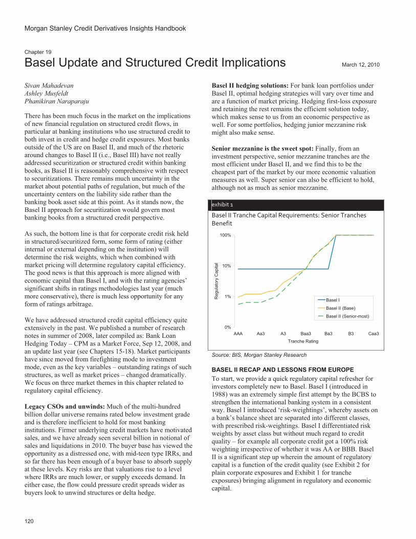
Morgan Stanley Credit Derivatives Insights Handbook
120
Chapter 19
Basel Update and Structured Credit Implications March 12, 2010
Sivan Mahadevan Ashley Musfeldt Phanikiran Naraparaju
There has been much focus in the market on the implications of new financial regulation on structured credit flows, in particular at banking institutions who use structured credit to both invest in credit and hedge credit exposures. Most banks outside of the US are on Basel II, and much of the rhetoric around changes to Basel II (i.e., Basel III) have not really addressed securitization or structured credit within banking books, as Basel II is reasonably comprehensive with respect to securitizations. There remains much uncertainty in the market about potential paths of regulation, but much of the uncertainty centers on the liability side rather than the banking book asset side at this point. As it stands now, the Basel II approach for securitization would govern most banking books from a structured credit perspective.
As such, the bottom line is that for corporate credit risk held in structured/securitized form, some form of rating (either internal or external depending on the institution) will determine the risk weights, which when combined with market pricing will determine regulatory capital efficiency. The good news is that this approach is more aligned with economic capital than Basel I, and with the rating agencies’ significant shifts in ratings methodologies last year (much more conservative), there is much less opportunity for any form of ratings arbitrage.
We have addressed structured credit capital efficiency quite extensively in the past. We published a number of research notes in summer of 2008, later compiled as: Bank Loan Hedging Today – CPM as a Market Force, Sep 12, 2008, and an update last year (see Chapters 15-18). Market participants have since moved from firefighting mode to investment mode, even as the key variables – outstanding ratings of such structures, as well as market prices – changed dramatically. We focus on three market themes in this chapter related to regulatory capital efficiency.
Legacy CSOs and unwinds: Much of the multi-hundred billion dollar universe remains rated below investment grade and is therefore inefficient to hold for most banking institutions. Firmer underlying credit markets have motivated sales, and we have already seen several billion in notional of sales and liquidations in 2010. The buyer base has viewed the opportunity as a distressed one, with mid-teen type IRRs, and so far there has been enough of a buyer base to absorb supply at these levels. Key risks are that valuations rise to a level where IRRs are much lower, or supply exceeds demand. In either case, the flow could pressure credit spreads wider as buyers look to unwind structures or delta hedge.
Basel II hedging solutions: For bank loan portfolios under Basel II, optimal hedging strategies will vary over time and are a function of market pricing. Hedging first-loss exposure and retaining the rest remains the efficient solution today, which makes sense to us from an economic perspective as well. For some portfolios, hedging junior mezzanine risk might also make sense.
Senior mezzanine is the sweet spot: Finally, from an investment perspective, senior mezzanine tranches are the most efficient under Basel II, and we find this to be the cheapest part of the market by our more economic valuation measures as well. Super senior can also be efficient to hold, although not as much as senior mezzanine.
exhibit 1
Basel II Tranche Capital Requirements: Senior Tranches Benefit
0%
1%
10%
100%
AAA Aa3 A3 Baa3 Ba3 B3 Caa3
Tranche Rating
Reg
ulat
ory
Cap
ital
Basel I
Basel II (Base)
Basel II (Senior-most)
Source: BIS, Morgan Stanley Research
BASEL II RECAP AND LESSONS FROM EUROPE To start, we provide a quick regulatory capital refresher for investors completely new to Basel. Basel I (introduced in 1988) was an extremely simple first attempt by the BCBS to strengthen the international banking system in a consistent way. Basel I introduced ‘risk-weightings’, whereby assets on a bank’s balance sheet are separated into different classes, with prescribed risk-weightings. Basel I differentiated risk weights by asset class but without much regard to credit quality – for example all corporate credit got a 100% risk weighting irrespective of whether it was AA or BBB. Basel II is a significant step up wherein the amount of regulatory capital is a function of the credit quality (see Exhibit 2 for plain corporate exposures and Exhibit 1 for tranche exposures) bringing alignment in regulatory and economic capital.

Section C, Chapter 19 Basel Update and Structured Credit Implications
121
exhibit 2
Basel II Corporate Risk Capital Requirements: Aligning Regulatory and Economic Capital
0%
2%
4%
6%
8%
10%
12%
14%
16%
AAA Aa3 A3 Baa3 Ba3 B3Rating
Reg
ulat
ory
Cap
ital
Basel IFoundation IRBAdvanced IRB
Note: IRB – Internal Ratings Based Approach. Source: BIS, Morgan Stanley
While Basel II is new to US, Europe banks have already been under implementation of Basel II since 2008. As is clear from the discussion above, banks with a greater proportion of IG assets may actually end up reducing the risk-weighted assets. In a world where banks err towards more liquid and higher quality credit and have greater amount of buffers, Basel II could end up being more favorable from the asset perspective. There are also liability side implications (in terms of what constitutes capital) which we do not address here.
If the European Banks’ experience is any indicator, most large banks will ultimately seek approval from regulators to use the Advanced Internal Ratings Based Approach (AIRB). AIRB specifies methods to calculate the risk weighting based on internal estimates of the Probability of Default (PD), Exposure at Default (EAD) and Loss Given Default (LGD).
Because Basel II regulatory capital is closely aligned to the economic capital, changes in market pricing can influence strategies to a greater extent than under Basel I, as we will discuss later on. While senior tranches generically benefit relative to junior tranches, relative value perceptions – for example, between junior mezz and senior mezz or between senior and super senior – can change based on the pricing.
STRUCTURED CREDIT SWEET SPOT From an investment perspective, we update our analyses of the attractiveness of index tranches as measured by the spread per regulatory capital, keeping in mind the more stringent rating criteria (see Exhibit 3). For example IG13 10%-15% could potentially be a single ‘A’ rated tranche which attracts a risk weighting of 20%, implying regulatory capital of 1.6% of the notional (i.e., risk weight * capital ratio) of 8%. With current spread in the 100bp context, that translates into a spread per capital of 64%.
exhibit 3
Spread per Regulatory Capital for Index Tranches
S9 S9 3Y S9 5Y S9 7Y S9 10Y3-6% 4% 4% 5% 6%6-9% 26% 29% 15% 4%9-12% 21% 69% 38% 11%12-22% 17% 30% 47% 22%22-100% 8% 25% 46% 53%
IG13 IG13 3Y IG13 5Y 3-7% 4% 5% 7-10% 55% 30% 10-15% 32% 64% 15-30% 16% 26% 30-100% 9% 24%
IG9 IG9 3Y IG9 5Y IG9 7Y IG9 10Y3-7% 3% 8% 10% 11%7-10% 50% 14% 4% 6%10-15% 16% 35% 21% 5%15-30% 7% 21% 34% 19%30-100% 8% 22% 44% 59%
Bespokes*
Rating Tranche Portfolio1~ Tranche Portfolio2¬BB 4.5 - 6.5% 22% 4.2% - 6.2% 18%BBB 6.5 - 8.5% 92% 6.2% - 8.2% 77%A 8.5 - 11.0% 269% 8.2% - 10.5% 175%AA 11.0 - 15.0% 217% 10.5% - 14.5% 92%AAA 15.0 - 20.0% 125% 14.5% -17.5% 52% Note: * 100% IG portfolios 5yr maturity. ~ 80% US Name Portfolio. ¬
80% European name portfolio. Source: S&P, Morgan Stanley Research
Since we last published a similar table, we have had a continuation of a recovery in the belly of the capital structure – earlier the most attractive tranches from a long perspective. Given today’s changed pricing, the 9-100% part of the capital structure in iTraxx S9 7yr and 22-100% tranche in iTraxx S9 10yr seem to be the most attractive longs. iTraxx S9 7yr and 10yr 3-9% seem the least attractive tranches from a Basel II perspective. CDX IG13 5yr 7-15% seems to be the most attractive from a long perspective whereas 3-7% seems to be the least attractive part of the capital structure.
Across CDX IG9 7yr and 10yr, the 15-100% part of the capital structure seems to be most attractive from a long perspective, whereas 7-10% seems to be the least attractive part of the capital structure. We exclude equity tranches from this analysis given their full deductions under the capital model.
Finally, we run the same analysis on two examples of a potential new issue bespoke transaction with 5yr maturity. Both these portfolios are 100% IG underlying, one with a Euro centric portfolio and the other with a US centric portfolio. As seen in Exhibit 2, A/AA tranches are the new

122
sweet spot from a long perspective. Between the super senior (AAAs) and junior mezz (BBBs), relative value is less obvious and is likely to be sensitive to changes in market pricing.
LEGACY BESPOKE CSO MARKET As far as the bespoke CSOs from the last cycle are concerned, they are deeply underwater from a ratings perspective, as we have highlighted previously (see Exhibit 4). The sub-IG share jumped from under 5% at start of 2008, to 45% at the start of 2009 (post Lehman and Icelandics) and now stands at 81% (after the ratings methodology changes implemented in the second half of 2009). Clearly, these mostly mezzanine CSOs look unfavorable under Basel II. Despite their having the poor ratings problem for sometime now, unappetizingly low valuations were a key impediment for sellers early in 2009, as was a lack of an organized buyer base and lack of adequate depth.
exhibit 4
Legacy Bespoke CSOs – Largely Below IG Now
3% 5%
36%43% 46% 49% 52% 57% 58% 60% 61%
81% 81%
10%15%
18%
18% 16%15%
14%12% 12% 13% 13%
7% 7%
12%
14%
8%
7% 7% 6% 6%6% 7% 6% 6%
6% 6%
32%
30%
15%13% 13% 12% 11% 10% 9% 9% 8%
3% 3%
43%37%
23% 19% 18% 18% 17% 15% 15% 13% 13%3% 3%
0%
10%
20%
30%
40%
50%
60%
70%
80%
90%
100%
Nov-07
Aug-08
Nov-08
Dec-08
Jan-0
9
Feb-09
Mar-09
Apr-09
May-09
Jun-0
9Ju
l-09
Nov-09
Jan-1
0
AAAAAABBBSub-IG
Source: S&P, Morgan Stanley Research
A year ago, there was perhaps more imperative for restructuring (to improve portfolios and subordination in a still wide spread environment with less stringent rating criteria), but with stronger markets today, selling is now the more relevant theme. As we approach the tightest spread levels since the crisis, there seems to be greater willingness by sellers to ‘take profits’ after hanging on through the crisis.
It is hard to estimate how much will eventually be sold, as data in this part of the market is weak and unreliable, but we do believe that the stronger the underlying credit performance (particularly with many of the distressed financials that are in these portfolios), the more sellers will emerge. All that said, we would not completely write off restructuring as a solution for investors. Certainly, retracing the ratings slide back to AAA/AA through restructuring is a
herculean task with the new stringent ratings criteria. Nevertheless, restructuring is a viable alternative as long as the goals are not too ambitious. Just targeting a move of few notches from B to BB- or from BB to BBB- makes a material difference to the amount of capital held in absolute terms under Basel II, but would not cost that much in today’s tighter spread environment.
The predominant nature of this risk was originally mezz like but is more equity/junior mezz like today. We expect to see widening pressure on the junior parts of the capital structure as a result of potential unwinds, but a maturing ratings-insensitive buyer base has developed in 2009 and should be able to absorb these sales as they occur. Orderly CSO BWICs are a regular occurrence today and appetite for secondary CSO paper remains fairly strong for now.
SECURITIZATION AND CAPITAL RELIEF STRATEGIES Last but not least, securitization and capital relief strategies have experienced a complete U-turn from Basel I to Basel II. The most common Basel I strategy involved retaining the yieldiest part of the capital structure, i.e., the equity tranche, and buying protection on 3-100% part of the capital structure. Under Basel II, the optimal strategies for Europe proved to be the exact opposite – the focus is on what part of the capital structure is most efficient to retain, and as we discussed above, it is really the senior, higher quality tranches that were the most attractive risk to retain. Investors have a number of types of hedging choices (see Exhibit 5).
Based on simulation of various hedging alternatives (see Chapter 16 for a detailed discussion of our methodology), we identified the following as the most optimal hedging strategies for CDX IG13 type portfolio (see Exhibit 6):
� Retaining senior risk (x-100%) is good, where the attachment is 4% based on today’s market pricing for CDX IG type portfolios. The optimal attachment has drifted up from 2% since we last discussed this (see Chapter 18).
� This analysis is based on the relatively cleaner IG13 portfolio. As the quality of the portfolio becomes lower, the higher the optimal attachment moves. For example, when we first ran this analysis in 2008, retaining X-100% was optimal for both IG and LCDX portfolios. Whereas ‘X’ was around 2% to 4% for IG portfolios, it was 9% to 12% for leveraged loan portfolios.
� For the wider spread portfolios, both equity and junior mezz look good to hedge today. It seems the key hedging decision for many investors is whether to hedge equity tranches or mezzanine or even both. This decision will be a function of the portfolio, yield targets, and hedging capacity of investors.

Section C, Chapter 19 Basel Update and Structured Credit Implications
123
CONCLUSION As valuations reach the tightest levels we have seen in two years now, we see renewed focus and debate on longer term drivers and what will influence the fair value of credit. Given that banks and financial institutions are amongst the primary investors for credit, the regulatory regime and capital requirements across various types of assets will be an important driver of pricing of credit in both an absolute and relative sense within the tranche capital structure.
exhibit 5
Thinking about Structured Hedging Alternatives
Long Index
5-100% tranche risk retained
Equity tranche (0-5%) hedged
9-100% tranche risk hedged
Equity tranche (0-5%) hedged
5-9% retained
9-12% hedged
Equity tranche (0-5%) hedged
12-100% tranche risk retained
5-9% retained
2T – H-L
3T – H-L-H
4T – H-L-H-L
Sell Protection on 5-100% tranche risk
Equity tranche (0-5%) No position
2T – N-L
Source: Morgan Stanley Research
exhibit 6
Hedging Equity Risk More Optimal Than Outright Longs or Hedging Senior Risk
0%
20%
40%
60%
80%
100%
120%
140%
0% 2% 4% 6% 8% 10% 12%
Equity Tranche Detachment
Spre
ad/R
egul
ator
y C
apita
l
Index (2008)2T-L-H (2008)2T-H-L (2008)Index (2010)2T-L-H (2010)2T-H-L (2010)
Note: 2T L-H means split portfolio in two parts and retaining equity (0-x%) and hedging x-100%. (See Exhibit 5).
Source: S&P, Morgan Stanley Research

124

Section D
The Legacy CSO Market
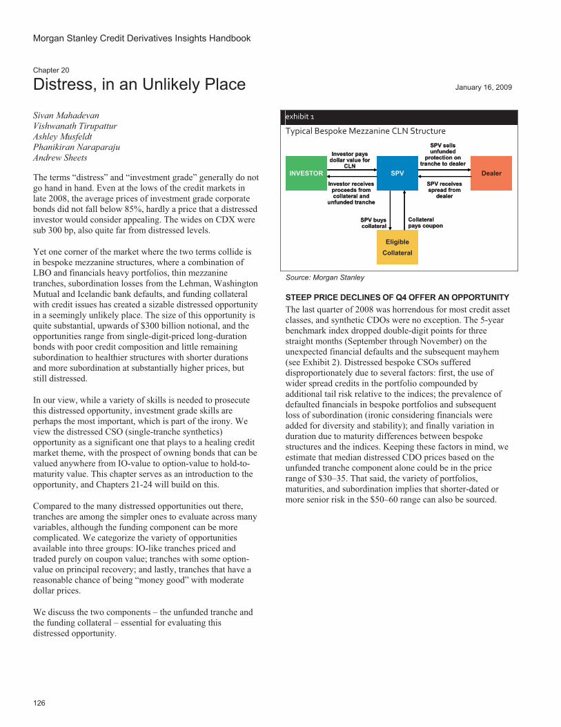
Morgan Stanley Credit Derivatives Insights Handbook
126
Chapter 20
Distress, in an Unlikely Place January 16, 2009
Sivan Mahadevan Vishwanath TirupatturAshley Musfeldt Phanikiran Naraparaju Andrew Sheets
The terms “distress” and “investment grade” generally do not go hand in hand. Even at the lows of the credit markets in late 2008, the average prices of investment grade corporate bonds did not fall below 85%, hardly a price that a distressed investor would consider appealing. The wides on CDX were sub 300 bp, also quite far from distressed levels.
Yet one corner of the market where the two terms collide is in bespoke mezzanine structures, where a combination of LBO and financials heavy portfolios, thin mezzanine tranches, subordination losses from the Lehman, Washington Mutual and Icelandic bank defaults, and funding collateral with credit issues has created a sizable distressed opportunity in a seemingly unlikely place. The size of this opportunity is quite substantial, upwards of $300 billion notional, and the opportunities range from single-digit-priced long-duration bonds with poor credit composition and little remaining subordination to healthier structures with shorter durations and more subordination at substantially higher prices, but still distressed.
In our view, while a variety of skills is needed to prosecute this distressed opportunity, investment grade skills are perhaps the most important, which is part of the irony. We view the distressed CSO (single-tranche synthetics) opportunity as a significant one that plays to a healing credit market theme, with the prospect of owning bonds that can be valued anywhere from IO-value to option-value to hold-to-maturity value. This chapter serves as an introduction to the opportunity, and Chapters 21-24 will build on this.
Compared to the many distressed opportunities out there, tranches are among the simpler ones to evaluate across many variables, although the funding component can be more complicated. We categorize the variety of opportunities available into three groups: IO-like tranches priced and traded purely on coupon value; tranches with some option-value on principal recovery; and lastly, tranches that have a reasonable chance of being “money good” with moderate dollar prices.
We discuss the two components – the unfunded tranche and the funding collateral – essential for evaluating this distressed opportunity.
exhibit�1�
Typical�Bespoke�Mezzanine�CLN�Structure�
Investor pays dollar value for
CLN
Investor receives proceeds from collateral and
unfunded tranche
INVESTOR SPV
EligibleCollateral
SPV buys collateral
Collateral pays coupon
Dealer
SPV sells unfunded
protection on tranche to dealer
SPV receives spread from
dealer
Investor pays dollar value for
CLN
Investor receives proceeds from collateral and
unfunded tranche
INVESTOR SPV
EligibleCollateral
SPV buys collateral
Collateral pays coupon
Dealer
SPV sells unfunded
protection on tranche to dealer
SPV receives spread from
dealer
Source: Morgan Stanley
STEEP PRICE DECLINES OF Q4 OFFER AN OPPORTUNITY The last quarter of 2008 was horrendous for most credit asset classes, and synthetic CDOs were no exception. The 5-year benchmark index dropped double-digit points for three straight months (September through November) on the unexpected financial defaults and the subsequent mayhem (see Exhibit 2). Distressed bespoke CSOs suffered disproportionately due to several factors: first, the use of wider spread credits in the portfolio compounded by additional tail risk relative to the indices; the prevalence of defaulted financials in bespoke portfolios and subsequent loss of subordination (ironic considering financials were added for diversity and stability); and finally variation in duration due to maturity differences between bespoke structures and the indices. Keeping these factors in mind, we estimate that median distressed CDO prices based on the unfunded tranche component alone could be in the price range of $30–35. That said, the variety of portfolios, maturities, and subordination implies that shorter-dated or more senior risk in the $50–60 range can also be sourced.

Section D, Chapter 20 Distress, in an Unlikely Place
127
exhibit�2�
5yr�Index�Junior�Mezz�Monthly�Performance�
-25%
-20%
-15%
-10%
-5%
0%
5%
10%
15%
20%
25%
May
-07
Jun-
07
Jul-0
7
Aug
-07
Sep
-07
Oct
-07
Nov
-07
Dec
-07
Jan-
08
Feb-
08
Mar
-08
Apr
-08
May
-08
Jun-
08
Jul-0
8
Aug
-08
Sep
-08
Oct
-08
Nov
-08
Dec
-08
Jan-
09Source: Morgan Stanley Research
We broadly divide distressed opportunities into three groups:
IO-Value. These are the really low-dollar-price instruments, (below $10), which are priced like IOs – typically equal to about 2-3 years of coupon. It is expected that the principal value will be little to nothing at maturity; the valuation is done based on expectations of how many coupons the structure will pay out before the notional goes to zero. The yield to maturity of these structures would be in the 60+ range.
Option-Value. These are mid-priced structures ($5–30) that capture the interest component plus the small chance of principal recovery. Yields for these deals are likely in the 30-60% range.
Money-Good. These structures can have any or all of the following: shorter maturities, cleaner portfolios, higher subordination, and greater thickness. Consequently they have higher associated prices ($20–60). These are categorized as money-good because while nowhere near a certainty, the likelihood that there will be at least a partial principal repayment is high. Yields here are much lower (25–50%) but still fairly attractive compared to the high-single-digit and low-to-mid-teen risk-adjusted returns for plain vanilla IG/loans or HY credit. There are obviously more risk remote tranches as well.
exhibit�3�
Synthetic�CDO�Market�Overview�
Nov-07 Aug-08 Nov-08Deal Type Synthetic CDO of CDO 642 639 618Synthetic CDO 2217 2,395 2072Total 2,859 3,034 2,690Management Type Managed 47.1% 49.9% 52.3%Static 43.8% 40.7% 38.4%Hybrid (lightly managed, etc.) 9.2% 9.4% 9.2%Original Rating Category AAA 44.8% 44.9% 45.1%AA 34.1% 33.2% 34.6%A 11.7% 11.9% 11.4%BBB 7.1% 7.6% 6.8%Sub-Investment Grade 2.2% 2.4% 2.0%Current Rating Category AAA 42.6% 37.1% 22.8%AA 32.0% 30.1% 15.1%A 12.5% 13.5% 8.1%BBB 10.0% 14.5% 18.3%Sub-Investment Grade 2.9% 4.8% 35.8%Geography Europe 52.7% 51.6% 55.1%Asia 11.9% 11.5% 12.6%North America 35.4% 36.9% 32.3%
Source: Morgan Stanley Research
RATINGS BECOMING LESS RELEVANT Tranche ratings, already under pressure from defaults and negative rating transitions in the underlying portfolios, are also being affected by more stringent ratings criteria announced in the last several weeks. However, ratings are becoming less relevant, given that the dollar prices have approached significantly distressed levels over the course of the last quarter. Furthermore, the credit universe has already transitioned dramatically from a median AA-rated universe in 2007 to a BBB/Sub-IG-heavy universe in the post-Lehman environment (see Exhibit 3). With the added impact of the rating criteria revisions, we expect the investor base to do one of three things: reconcile themselves to holding non-IG tranches given deeply distressed prices (most likely), restructure to enhance ratings (less likely) or attempt to liquidate at current prices (somewhat likely). Meanwhile, banks that were set up to inventory these products are faced with decreased risk-taking capacity of their own. We estimate at least $300 billion notional is still outstanding and from Exhibit 3, we can see that the number of deals outstanding has decreased about 10% since August 2008. Some of this risk may be owned by dealers now, but we believe the bulk of this risk is still in the hands of structured investors.
STRUCTURAL VALUATION OF THE UNDERLYING TRANCHE Taking advantage of this dislocation requires some background knowledge of the market, though we stress that sophisticated correlation models aren’t as necessary here as

Morgan Stanley Credit Derivatives Insights Handbook
128
they were earlier. We break down the tranche valuation aspect into several components.
Subordination. Many of the 2008 defaults were common names in bespoke CLNs, which tend to be entirely IG names. The GSEs, Lehman, Washington Mutual, and the Icelandic banks in particular were popular constituents of these structures, and thus many of the structures out there have had at least some write-down. What’s important is what’s left in the portfolio and how many additional losses can be sustained.
Thickness. Thin tranches were the dominant theme when these assets were originally structured, to increase structural leverage and thus spread. This matters because if the CLN is touched at all, it could require only one additional default to wipe out the entire tranche. This is very different from the index tranches, which are all at least 3% thick and can withstand a greater number of defaults once breached.
Portfolio composition. This is clearly important, particularly if there is little subordination left in the structure. We have written extensively about tails and portfolio dispersion in the past, usually concerning the various index series. It is no less important here when evaluating bespoke structures and indeed the valuation methodology is largely the same.
While it is hard to generalize the different portfolios out there, S&P recently published a list of the top 100 corporate obligors out of approximately 450 corporate obligors referenced in roughly 1,000 US synthetic CDOs, giving the market a very good sense of what a typical portfolio could look like (see Exhibit 4). These 100 names represent about half of the total corporate exposure in US deals. While the tail risk for different CDO portfolios would vary significantly, it is fair to say that the belly and the left tail have similarities across portfolios. Often the portfolios would be wider-spread portfolios than the index at inception and that continues today. A typical CDO portfolio spread currently could be in the 500-700bp range, i.e., almost 2x the spread of the CDX index, with the 10% tail contributing 40% or more of the index spread (though tight spread portfolios are common). The exact attachments vary but an original AAA tranche would likely attach in the high single digits and have a 1% thickness, with a price under 20%.
To combat some of the extreme dispersion present in these portfolios, we like paying for risk management and recommend using some amount of the coupon income to pay for a manager and/or buying protection on tail names.
exhibit�4�
What�Do�Typical�Portfolios�Look�Like?�
0%
5%
10%
15%
20%
25%
30%
100
200
300
400
500
600
700
800
900
1000
1100
1200
1300
1400
1500
>150
0
CDO 1 (Avg 715bp)CDO2 (Avg 514bp)All Credits (Avg 615bp)
Source: Morgan Stanley Research
Recovery. The majority of these structures are floating recovery, and as we’ve seen lately, particularly with respect to Tribune, recovery can be very low on certain names. Some, however, are fixed recovery, generally 40%, and this added certainty regarding number of defaults needed to impact the tranche can be very valuable.
Managed or static. Some CLNs are managed synthetics, and the added presence of a manager can be valuable, depending on the manager.
Maturity. The five-year maturity deals done in 2004/2005 have very short maturities and yet some are still trading at highly distressed levels. Alternatively, in 2006/2007 most CLNs were structured with 7- and 10-year maturities, as investors shunned the shorter maturities in a reach-for-yield environment characterized by steep spread curves. Today, with curves flat or inverted, we argue that maturity is far less important than the first five components listed above, though still worth noting, particularly in the very short end.
Coupon. While we argue that the deeply discounted dollar price is the more eye-catching price component, for those bespokes we consider to fall under the category of “IO opportunity,” coupon is important.

Section D, Chapter 20 Distress, in an Unlikely Place
129
exhibit�5�
Top�100�Names�vs.�CDX�
0
100
200
300
400
500
600
Mar-06 Sep-06 Apr-07 Nov-07 May-08 Dec-081.0
1.2
1.4
1.6
1.8
2.0
2.2
2.4
2.6
Top 100 CDO Credits IndexCDX IG ROTRRatio of CDO basket spread/CDX
Source: Morgan Stanley Research
COLLATERAL VALUATION While analyzing the underlying corporate portfolios is something that most investment grade investors ought to be comfortable with, the collateral component may be a little less familiar.
In these synthetic funded CDO structures, a wide variety of collateral has been used over time, ranging from money market instruments, to asset-backed paper (credit cards), to covered bonds and beyond. There is some discrepancy in collateral performance with some trading at a significant discount, while others are still trading at or near par. MMF
and covered bond collateral both score high in our view, as they have performed reasonably well so far, whereas we are wary of GICs or other structured products.
Credit card AAAs are common collateral (see “Playing Your Cards Right” from October 30, 2008 for an overview of our thoughts) and are structurally well protected, despite the stresses in this form of consumer credit today. We also note that there is a significant variation in the composition of different credit card ABS trusts and this creates significant performance variation. A strong positive factor for this asset class is the potential support from TALF. Fed chairman Ben Bernanke, in a recent speech, suggested the Fed will begin a program to bolster securitization markets for consumer credit. The Term Asset-Backed Securities Loan Facility will finance up to $200 billion in securities backed by loans to small businesses, students, credit-card holders and car buyers. We hope to discuss different collateral types and valuation implication in subsequent research.
CONCLUSIONWith our views on a healing investment grade credit market globally, we feel that there is a significant opportunity today to prosecute what is perhaps the most distressed corner of the investment grade market, the several hundred billion dollar market for distressed synthetic CDOs. The opportunity is less about structure and more about credit, both the corporate credit backing the tranche and the collateral backing the credit-linked notes, and it is ultimately this skill set that is necessary to evaluate deals. We will devote additional research to evaluating these components together to find the best value among the opportunities out there.

Morgan Stanley Credit Derivatives Insights Handbook
130
Chapter 21
Getting a Handle on Distressed Mezz January 30, 2009
Sivan Mahadevan Ashley Musfeldt Phanikiran Naraparaju
In Chapter 20, we began our discussion of the current opportunity for investing in distressed bespoke mezzanine structures. This opportunity is several hundred billion dollars in size, and a good amount of risk needs to change hands given price and ratings actions. Since most deals have predominantly investment grade credit as the primary building block, we have argued and continue to stress that fundamental IG corporate credit analysis capabilities are probably the most important skill required to take advantage of this opportunity. Here, understanding jump-to-default and liquidity risks can be useful in bucketing companies into high-, medium- and low-risk credits and then assessing the potential residual life of the unfunded tranche component, given subordination and other structural features.
The ultimate potential gains from this distressed opportunity can be quite significant, especially considering the notion that many structures may ultimately mature with no realized losses given subordination levels and high quality funding collateral. However, picking the winners from the losers is challenging, and the cost of being wrong can be high, given the thinness of some of these tranches.
In this chapter, we dig deeper into the fundamental analysis, and combine this with a closer look at the funding component. When evaluating these two components together, it can be helpful to think of the entire structure as a first-to-default on the collateral and tranche together. If we evaluate the two parts individually, it is possible to come up with a conservative estimate for the ultimate value of the asset, since the likelihood of survival of each is probably related. To evaluate these assets, we break down our analysis into four parts.
Collateral: The wide variety of collateral available for funding these structures makes this a difficult component to generalize, but we highlight some of the important factors in the most common types of collateral in the market today. We stress that deal-specific factors can vary.
exhibit�1�
Typical�Bespoke�Mezzanine�CLN�Structure�
Investor pays dollar value for
CLN
Investor receives proceeds from collateral and
unfunded tranche
INVESTOR SPV
EligibleCollateral
SPV buys collateral
Collateral pays coupon
Dealer
SPV sells unfunded
protection on tranche to dealer
SPV receives spread from
dealer
Investor pays dollar value for
CLN
Investor receives proceeds from collateral and
unfunded tranche
INVESTOR SPV
EligibleCollateral
SPV buys collateral
Collateral pays coupon
Dealer
SPV sells unfunded
protection on tranche to dealer
SPV receives spread from
dealer
Source: Morgan Stanley
IO structures: In these assets, timing of defaults in the underlying portfolio and longevity of the collateral are the most important considerations. We highlight some of the unique features of an asset that is expected to have a low to zero maturity value.
Potentially money-good assets: Here, collateral is of utmost importance, and the investor should be much more comfortable with the portfolio and/or subordination. Hedging strategies for protection against extreme scenarios should be much cheaper.
Option-value assets: These are somewhere in between the two extremes; since they are still trading at highly distressed levels, overall survival of both the collateral and unfunded tranche should be more likely than for IO structures, though default timing and probabilities are less certain. Coupons, too, can vary in this type of asset.
GOOD COLLATERAL, BAD COLLATERAL Recall that when a credit-linked note (CLN) is created, the proceeds from the sale of the note are used to set up a special purpose vehicle (SPV), which purchases high quality collateral for funding purposes. The SPV then sells protection on the reference entity (for our purposes, a tranche) in unfunded form to the swap counterparty (dealer or CP). When these structures were originally created, the collateral was generally AAA-rated, with ratings cushion, and priced at par with a Libor-flat-like coupon. However, as the market in general has suffered, so have the specific underlying assets that generally make up the funding component. These encompass a variety of assets, including but not limited to: covered bonds, money market funds (MMFs), credit card ABS, GICs, corporate bonds, sovereign bonds (Treasuries, JGBs), agencies, and dealer repos. While we stress deal-specific factors are important, these assets are currently

Section D, Chapter 21 Getting a Handle on Distressed Mezz
131
valued in varying degrees of distress (prices range anywhere from 60-100 cents). We offer our general views on these as follows:
Credit-card ABS. Credit-card ABS are one of the most common types of funding for bespoke structures. The main considerations here are the issuer, composition of the security, and structural features. For instance, since many of these have a certain percentage of sub-prime borrowers, knowing what percentage is the key to evaluating the quality of the overall collateral. We estimate this collateral could be trading from the mid-60s to the mid-80s.
Guaranteed investment contracts. GICs can vary widely in terms of quality and price, depending on a number of factors, including who the issuer is, what thresholds are required to be breached before additional collateral is posted, and what additional collateral is permitted. Typically there is a certain ratings threshold that must be breached before the posting requirement comes into effect, so for example a GIC backed by GE would not currently have anything additional posted, since GE has maintained its AAA-rating. A GIC backed by a monoline, on the other hand, would have already dropped below the ratings threshold. The main consideration here is jump risk – the risk that any issuer would be downgraded faster than they could post the additional collateral required. While these benefit from the additional collateral requirements and triggers, they are considerably more opaque and difficult to price.
Corporate bonds. These are theoretically the easiest and most transparent to evaluate, though they introduce an element of idiosyncratic risk to the structure. They would have had a rating greater than or equal to the tranche rating at inception, so the majority were AAA-rated corporate bonds, such as GECC, Berkshire Hathaway, or a monoline. We would argue that duration is a key consideration.
Covered bonds. Covered bonds are somewhere in between agencies and senior financials in terms of the risk profile. These assets continue to be rated well (AAA/AA) and we are generally constructive on this type of risk due to government support for financial institutions. Nevertheless, there is a fair amount of dispersion in prices (from above par to 75 cents) depending on the duration of the bond and issuer.
ONE ASSET, TWO VALUATIONS Because collateral default leads to liquidation of the collateral and distribution of proceeds to the swap counterparty and the investor in that order, the first step in the valuation of these structures involves assessing which of the two elements – the tranche or the collateral – will outlast the other. In many cases, such as covered, agency, or sovereign bonds, the comfortable answer is that the collateral is highly likely to make it to tranche maturity. Most assets, however, are less clear and are highly deal specific. If the tranche is the weaker link, the valuation focuses on tail risk
vs. remaining subordination in the tranche. If the collateral is the weaker link, the valuation focuses on average life of the collateral and potential liquidation value of the collateral vs. the MTM on the unfunded tranche.
exhibit�2�
Sample�Distressed�Bespoke�Mezzanine�Assets�
Type Tranche
Type Cpn Maturity Price
(%) Yield to Maturity
PriceCoupon
Ratio IO-Value Mezz L+250 2014 3.0% - 0.8IO-Value Mezz L+160 2017 4.6% 61% 2.0IO-Value Mezz L+65 2014 5.4% 70% 3.1IO-Value Mezz L+430 2017 7.5% 77% 1.3IO-Value Equity L+1200 2013 11.0% - 0.8IO-Value Equity L+1600 2011 25.0% - 1.4Option-Value Mezz L+150 2012 8.0% 84% 3.1 Option-Value Mezz L+210 2013 13.3% 63% 4.2 Option-Value Mezz L+100 2013 16.0% 53% 7.7 Money-Good Senior L+140 2009 59.0% 66% 23.7Money-Good Senior L+121 2011 61.2% 26% 16.7Money-Good Senior L+121 2010 62.0% 28% 31.9Money-Good Mezz L+30 2010 70.0% 28% 52.4
Source: Morgan Stanley Research
In Exhibit 2, we provide a sampling of distressed bespoke mezzanine tranches in the market today. These vary in portfolio and collateral on a broader level, and across several more specific structural features as well. For instance, there are a few that have an off-market fixed recovery, making them more attractive than they would initially appear, while others have third-party managers, making the portfolio risk harder to determine upfront. From this information alone, it is difficult to assess relative value, but it does highlight the variety and depth of the opportunity.
exhibit�3�
Ratings�Distribution�of�100�Popular�Names�in�CDOs�
2%
5%
35%
39%
10%
5% 4%
0%
5%
10%
15%
20%
25%
30%
35%
40%
45%
AAA AA A BBB BB B CCC or below
Source: Morgan Stanley
PORTFOLIOS, SUBORDINATION AND PRICING Along with collateral analysis, assessing the portfolio risk is another crucial step in evaluating this opportunity. While

Morgan Stanley Credit Derivatives Insights Handbook
132
each asset has its own unique underlying portfolio composition, we do get some clarity on the general makeup of these assets by looking at a list published by S&P of the 100 most common names in bespoke mezzanine CDOs. We analyzed the portfolio characteristics of these credits for clues about the expected default rates for these portfolios and hence subordination requirements. Almost a fifth of the portfolio of these 100 common names is now rated below investment grade (Exhibit 3). Furthermore, sector composition is skewed heavily towards financials (including Insurers [26%] and Consumer Discretionary [24%]) followed by Telecom (13%). Many of the non-financials were bull-market-era LBO names. We applied the historical default rate for similar corporate portfolios (in terms of ratings distribution) and found that the worst case 5-year cumulative default rates for a similarly rated portfolio would be in the 8-9% context (Exhibit 4), nearly double that for CDX/iTraxx type portfolios. This puts credit losses in the 5–6% range, if we assume a conservative recovery of 30%.
Clearly the experience of individual deals would vary, but deals with less than five years of residual maturity and subordination in excess of 6% could expect at least some recovery of principal. The timing of subordination erosion also matters. For the deals in Exhibit 2, we calculate risk-adjusted IRRs assuming the majority of the expected defaults in the 5-year period occur in 2009 and 2010. These conservative estimates give IRRs in the 20-50% range.
exhibit�4�
Historical�Default�Rates�for�a�Typical�CDO�Portfolio�
0%
1%
2%
3%
4%
5%
6%
7%
8%
9%
1970
1972
1974
1976
1978
1980
1982
1984
1986
1988
1990
1992
1994
1996
1998
2000
2002
0%
1%
2%
3%
4%
5%
6%
7%
8%
9%5yr Cumulative Default RateAverage
Source: Morgan Stanley
Further, we would divide portfolios into three stratifications: 1) wide-trading names that are difficult to hedge and very binary; 2) wide-trading names where the outcomes are more skewed toward survival; and 3) healthier names that are more default remote. We believe that credits in the first camp should be “written-off” in a worst-case analysis to determine how much subordination is left in the structure and that credits in the second camp are candidates for active hedging in any distressed mezzanine investment strategy. For the third camp, these are credits that should be left unhedged and
represent the “hope” of the investment strategy. Investors will find that some of the IO-value tranches are timing plays on the wide end of this tail, and the option-value plays are more a survival bet on the tail.
VALUING IO-LIKE TRANCHES IO-like tranches, to reiterate, are those that derive the majority of their value from the coupon stream, since they are highly unlikely to return any principal. We pick a sample trade from the list in Exhibit 2, priced at 3% and a coupon of L+250bps with the maturity at least 5 years away. The asset is clearly not expected to survive until maturity, and the extreme tail risk in this sample portfolio is quite high. Nonetheless, this asset will break even in a year and half, and thus any additional coupon payments or value at maturity is excess return for the investor. The main focus is to collect the coupon for as long as possible, on the highest notional possible.
exhibit�5�
Sample�IO�Value�Portfolio�Spread�Distribution�
0
5
10
15
20
25
30
35
0-100 100-200
200-500
500-750
750-1000
1000-1250
1250-1500
1500-2000
2000+
Source: Morgan Stanley
Clearly, given a certain amount of subordination, portfolio composition is a key factor here, followed by timing of defaults. It is already assumed that there will be several defaults in the portfolio, and for most IO-value tranches, it is assumed that the tranche will be wiped out. This is where the fundamental credit skills become paramount – a view on the tails is critical. Since yields here are in the 60%+ range, we only need one out of five deals to survive longer than the breakeven period to achieve mid-teen returns and compare favorably to single-digit returns on IG credit or mid-teen returns for the HY universe.
POTENTIALLY MONEY-GOOD TRANCHES At the other end of the spectrum are higher-dollar-price tranches that are expected to be money good in most reasonable scenarios. These are often thicker tranches with higher subordinations, and cleaner portfolios or shorter maturities. For these assets, coupon and price take a backseat to the ultimate survival of both the tranche and the collateral. This is not to say that price and coupon are unimportant;
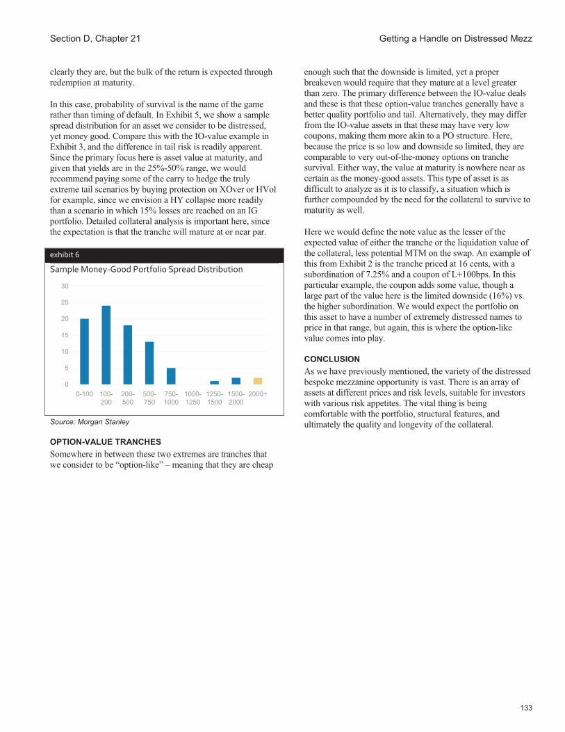
Section D, Chapter 21 Getting a Handle on Distressed Mezz
133
clearly they are, but the bulk of the return is expected through redemption at maturity.
In this case, probability of survival is the name of the game rather than timing of default. In Exhibit 5, we show a sample spread distribution for an asset we consider to be distressed, yet money good. Compare this with the IO-value example in Exhibit 3, and the difference in tail risk is readily apparent. Since the primary focus here is asset value at maturity, and given that yields are in the 25%-50% range, we would recommend paying some of the carry to hedge the truly extreme tail scenarios by buying protection on XOver or HVol for example, since we envision a HY collapse more readily than a scenario in which 15% losses are reached on an IG portfolio. Detailed collateral analysis is important here, since the expectation is that the tranche will mature at or near par.
exhibit�6�
Sample�Money�Good�Portfolio�Spread�Distribution�
0
5
10
15
20
25
30
0-100 100-200
200-500
500-750
750-1000
1000-1250
1250-1500
1500-2000
2000+
Source: Morgan Stanley
OPTION-VALUE TRANCHES Somewhere in between these two extremes are tranches that we consider to be “option-like” – meaning that they are cheap
enough such that the downside is limited, yet a proper breakeven would require that they mature at a level greater than zero. The primary difference between the IO-value deals and these is that these option-value tranches generally have a better quality portfolio and tail. Alternatively, they may differ from the IO-value assets in that these may have very low coupons, making them more akin to a PO structure. Here, because the price is so low and downside so limited, they are comparable to very out-of-the-money options on tranche survival. Either way, the value at maturity is nowhere near as certain as the money-good assets. This type of asset is as difficult to analyze as it is to classify, a situation which is further compounded by the need for the collateral to survive to maturity as well.
Here we would define the note value as the lesser of the expected value of either the tranche or the liquidation value of the collateral, less potential MTM on the swap. An example of this from Exhibit 2 is the tranche priced at 16 cents, with a subordination of 7.25% and a coupon of L+100bps. In this particular example, the coupon adds some value, though a large part of the value here is the limited downside (16%) vs. the higher subordination. We would expect the portfolio on this asset to have a number of extremely distressed names to price in that range, but again, this is where the option-like value comes into play.
CONCLUSIONAs we have previously mentioned, the variety of the distressed bespoke mezzanine opportunity is vast. There is an array of assets at different prices and risk levels, suitable for investors with various risk appetites. The vital thing is being comfortable with the portfolio, structural features, and ultimately the quality and longevity of the collateral.

Morgan Stanley Credit Derivatives Insights Handbook
134
Chapter 22
Restructuring Renaissance May 8, 2009
Sivan Mahadevan Phanikiran Naraparaju Ashley Musfeldt
The speed at which markets and psychology have turned recently should not be ignored, and many in the investment community are willing to look beyond near-term issues to an environment of slow economic growth and fundamental valuation opportunities. Investment grade credit will continue to measure up well by these metrics, and if companies have good business models and access to liquidity, then “large cap” default risk ought to shrink substantially as we move forward. The structured credit mezzanine machine of 2004-2007 was all about this theme, as investors bought levered tranches that could withstand a few defaults and safely return principal. This credit cycle has clearly thrown that investment thesis out the window, even though most of the several hundred billion dollars of mezzanine tranches in the market have yet to realize principal loss. So what should investors in this now-distressed part of the investment grade market do?
With the new CDS SNAC, we thought we’d gotten rid of the “Restructuring” lexicon from our vernacular, but restructuring of a different sort is back in vogue. In the last credit cycle (2001-2002), synthetic CDOs backed by combinations of IG and crossover credits were stressed, and while some investors sold, most ultimately hung on to their risks and restructured in many cases to ride out the storm. A high “fallen angel” default environment was responsible for triggering the stress, but post Sarbanes-Oxley, investment grade default risk fell materially, and a credit recovery ensued.
In this cycle, we have replaced stress with distress in bespoke mezzanine structures, and that difference has forced many to sell, along with other factors including a significantly weaker environment for financial institutions (the large buyers of synthetic CDOs) owing to systemic risk and capital needs. As such, we have been fairly vocal about our expectation of more selling this time around, which combined with valuations is one of the reasons we continue to believe that bespoke mezzanine is among the most interesting distressed opportunities in the market. However, we are also seeing motivation to restructure deals, as many investors turn more constructive on risk markets and feel that adding capital may result in a healthier total return rather than selling today.
We believe the market is big enough to make both opportunities (buying distressed and restructuring existing transactions) feasible and attractive. The opportunity to restructure is perhaps better in the current environment (with spreads and distressed tails still wide) than it would be in a
much healthier environment, so timing is important. We devote this chapter to better understanding how restructuring is less expensive than one would guess, and how increasing ratings from B-rated to BB or BBB is both attractive price-wise and valuable from a capital perspective (for banks and insurance companies). We caution that one potential downside of restructuring is that the portfolio could continue to deteriorate meaningfully from a ratings or default perspective, resulting in a loss not only of original principal, but additional restructuring capital as well. Thus, having a constructive view on a large part of the portfolio is important. Furthermore, we highlight that any capital spent on restructuring is effectively realizing a cost upfront that won’t be returned, even if the tranche matures at par.
WHY IS NOW A GOOD TIME TO RESTRUCTURE? Why is an environment of wide spreads and a still-wide tail of credits a good time to restructure? The answer is that market-implied losses on credit are still high, but an inflection in the cycle now gives us more confidence in stating that actual losses from default may be significantly lower than what is implied.
exhibit�1�
S&P�500�–�Deep�OTM�Calls�Have�Similar�Prices�
0
10
20
30
40
50
60
97510
0010
2510
5010
7511
0011
2511
5011
7512
0012
2512
5012
7513
0013
2513
5013
7514
0014
2514
5014
7515
0015
2515
5016
00
S&P 500 Strike
Cal
l Pric
e (D
ec 0
9 Ex
piry
)
Source: Morgan Stanley, S&P
We use a simple options example to illustrate. The S&P 500 index is at about 900 today, and the market peak was just above 1500. If an investor had purchased an ATM 1500 strike call option near the peak, it would have been very expensive. Today that option is very cheap, but more importantly, an option with a 1200 strike is also very cheap (assuming a Dec-09 expiry). So an investor with a bullish view who does not believe that 1500 is attainable could restructure the 1500 strike call to a 1200 strike for a relatively small cost and own an option that seems more valuable, even though a risk-neutral derivatives pricing

Section D, Chapter 22 Restructuring Renaissance
135
model would not agree. If the S&P 500 were to rally to 1100, the 1200 strike option would be very expensive even though the 1500 strike option would likely still be cheap.
RATINGS, REAL-WORLD LOSSES AND PRICING We cite pricing from the equity market’s most liquid options to illustrate a complex point. If a credit portfolio has a 22% expected loss (implied by CDS curves and spreads), a 5-6% tranche is very OTM from a survivability perspective. So is an 8-9% tranche, but one’s real-world view of probability of loss can be meaningfully different for an 8-9% tranche than a 5-6% tranche, and the cost of moving up to it is not that significant today. It will be significant if spreads rally, curves steepen, and tails compress and the expected loss falls from 20% to 10% (which is still wider than when the mezzanine tranche was likely purchased).
exhibit�2�
Required�Attachment�Points�for�Sample�Portfolios�
Maturity: Jun 2014 Maturity: Jun 2016
Rating New S&P
Model Attach Old S&P
Model Attach New S&P
Model AttachOld S&P
Model AttachAAA 17.5% 11.9% 20.2% 13.0%AA+ 15.0% 11.5% 17.5% 12.6%AA 14.0% 10.9% 16.4% 12.1%AA- 13.0% 10.7% 15.3% 11.8%A+ 12.3% 10.5% 14.6% 11.5%A 11.8% 10.3% 14.0% 11.3%A- 10.9% 10.0% 12.9% 10.9%BBB+ 10.3% 9.5% 12.1% 10.5%BBB 9.8% 9.0% 11.5% 9.9%BBB- 9.1% 8.2% 10.7% 9.1%BB+ 8.5% 7.9% 10.1% 8.8%BB 8.1% 7.5% 9.5% 8.3%BB- 7.5% 7.1% 8.9% 7.9%B+ 7.0% 6.8% 8.4% 7.5%B 6.6% 6.4% 7.9% 7.1%B- 6.0% 6.0% 7.3% 6.6%CCC+ 5.5% 5.1% 6.7% 5.7%CCC 5.0% 4.5% 6.1% 5.2%CCC- 4.7% 3.7% 5.8% 4.3%
Source: Morgan Stanley, S&P
We also note that the ratings of an 8-9% tranche can be much better than a 5-6% tranche, given that rating agencies consider real-world losses, not risk-neutral. Restructuring adds value due to the disconnect between ratings, capital charges, real-world loss expectations vis-à-vis the market models and pricing.
ADDING SUBORDINATION IS NOT AS EXPENSIVE TODAY At its most basic, adding subordination simply involves taking the PV of the original tranche, subtracting from it the PV of the tranche with higher subordination, and paying the difference. Taking the example of a portfolio with a high expected loss (say 20-25% range), we examine the mechanics of an actual restructuring. Say the investor had a
tranche that was originally 6.5-7.5% and AAA-rated at inception. After several defaults and downgrades on the portfolio, this tranche is now 5-6% and rated CCC- (see Exhibit 3). Clearly this tranche is substantially underwater, with an attachment point of less than a quarter of the expected loss on the portfolio. If the investor has a market view on overall losses, or even a view on the tail names, one solution is to add subordination – not to anywhere near the expected loss, but simply a few percentage points higher, where the investor sees a significantly reduced probability of impairment.
exhibit�3�
Cost�of�Adding�Subordination�
Cost of Adding Subordination
0.0%1.0%2.0%3.0%4.0%5.0%6.0%7.0%8.0%9.0%
10.0%
0% 4% 8% 12% 16% 20% 24% 28% 32% 36%
Tranche Attachment Point (%)
Source: Morgan Stanley Note: Change in PV of the tranche by adding 1% of additional
subordination, divided by the PV of the original tranche
In Exhibit 3, we illustrate that as subordination is added closer to the expected loss (around 20% attachment) the cost gets higher, but that further away from the expected loss (around 7% attachment), the cost is much more manageable. This is shown by calculating the PV difference of the original tranche and the new, higher tranche, as a percentage of the original tranche’s PV. One interesting thing to note is that the distribution is considerably less predictable at the very low part of the capital structure – this is due to the lumpy tail distribution that disproportionately affects the equity tranche. In this particular portfolio, approximately 10% of the names are wide enough to be considered tail names, and the effect of these names on the equity tranches is quite significant.
In fact, it is not until we get to around 11%, or half the expected loss, that we start to see the distribution even out meaningfully. In addition to shoring up additional protection from portfolio losses at a relatively low cost, there is an ancillary benefit to additional subordination: improved tranche ratings. Continuing with our previous sample portfolio with a 22% expected loss, the 5-6% tranche is now CCC- by the old S&P model, and using the new criteria, would not even hit the CCC- threshold (see Exhibit 3). If the investor chose to add, say, 3% subordination and make the tranche an 8-9% tranche instead, this would boost the rating

Morgan Stanley Credit Derivatives Insights Handbook
136
from nonexistent to B in the new model and from CCC- to a BB- in the old model. For some investors, this jump can have real economic implications in the form of reduced capital requirements.
exhibit�4�
Cost�vs.�Capital�Benefits�of�Adding�Subordination�(Basel�II)�
0%
10%
20%
30%
40%
50%
60%
70%
80%
90%
100%
AAA AA+ AA AA- A+ A A- BBB+ BBB BBB- BB+ BB BB-
Rating after restructuring
% o
f Tra
nche
Not
iona
l
Cost for BB+ Cost for BB Cost for BB- Cost for BBenefit for BB+ Benefit for BB Benefit for BB- Benefit for B
Source: Morgan Stanley
WEIGHING BENEFITS VS. COSTS UNDER BASEL II The benefits of the restructuring are two-fold, one being the reduced riskiness in a real-world sense for the investor (as we discussed earlier) and the second is reduction in actual capital requirement. In our example, we go from a 5-6% tranche, which is below CCC-, to an 8-9% tranche, which is B rated. This is valuable subordination in the investor’s eyes, although it does not result in reduction in capital under Basel II (see Exhibit 4). For this additional subordination and ratings jump, the investor would pay about 10% of the tranche notional, so $1mm for a $10mm tranche. Adding a bit more subordination (1-2%) to go from B/CCC to a BB- tranche, however, can significantly reduce the capital required to be held against such an asset, up to half the tranche notional (Exhibit 4). This would cost another 5% in tranche notional or $0.5MM for $10MM tranche. While these amounts seem large, they are dwarfed by the benefit of capital requirements and improved likelihood of the tranche’s survival.
While it does cost a bit more, the capital benefits of improving a BB- rated tranche to a BBB are quite valuable – as much as 44% of the tranche notional in additional capital relief. If the investor were improving a B-rated tranche to an investment grade BBB- (8% attachment to 11% in our scenario), the charge would be roughly equivalent (usually, it would be more except for the lumpy tail in our sample portfolio) – or $1mm to go from a B to a BBB-. To go from an 8% attachment to a 14% attachment, the charge would be about 16%, or $1.6mm on a $10mm portfolio. In all these cases, the benefit outweighs the cost.
SUBORDINATION VS. PORTFOLIO AND MATURITY CHANGES Aside from adding subordination, another way to improve the PV of a tranche along with its ratings is to eliminate some of the widest or most concerning tail names. In a way, this is similar to the ratings optimization exercises that may have taken place when these transactions were originally structured. The issue today is that depending on the spread of the name to be removed compared to its replacement, the cost is quite a bit higher today, given the extreme levels of some tail names. In our sample portfolio, removing one of the widest names and replacing it with a name on the tighter part of the spread distribution would cost a little under $150k for a $10MM notional tranche. Substituting two names would end up, in this very specific instance, costing roughly the same as buying 1% additional subordination, and the benefits of doing one type of restructuring over the other would be portfolio, tranche, and name specific. Furthermore, it is possible that there are some names that could be swapped for a higher-rated name for little cost, though we do see investors moving away from looking at ratings as the sole measure of portfolio riskiness. The important thing to highlight in this round of restructurings is that we no longer see investors relying as heavily on name substitutions as in the past.
Restructuring in most cases involves additional cost, which is usually plugged by adding cash but also by generating value though maturity extension. In today’s inverted curve environment, extension is less juicy. On the contrary, investors might explore adding cash to reduce the maturity of the transaction in line with the better sentiment/confidence for near-term default risk generally in this rally.

137
Chapter 23
From Distressed to Just Stressed January 22, 2010
Sivan Mahadevan Ashley Musfeldt Phanikiran Naraparaju
A year ago, we called it “Distress, in an Unlikely Place” (see Chapter 20). The legacy bespoke mezzanine portion of the structured credit market was the victim of a combination of LBOs and financials, thin tranches, losses from actual defaults, and funding collateral concerns. Deals structured with mostly investment grade credit risk had morphed into a $300 billion distressed opportunity, and few investors had the skills to dig through the wreckage to sort out risk and find value. Structures with coupons ranging from L+30bp to L+500bp and maturities from a few months out to about 8 years were trading at levels as low as 1% to as high as about 70%.
In the year hence, several things happened. More defaults forced additional losses of subordination in some mezzanine tranches with a handful experiencing a total loss. However, at the same time, the most powerful rally in credit market history along with an outperformance of mezzanine-type risk caused some assets to enjoy price jumps of 10 to 60 points, with some shorter-dated deals even maturing at par. A buyer base for distressed CSOs emerged as well, equipped with simple methodologies for identifying value and forming a view on the tail credits.
Today, the distressed opportunity has not disappeared as many sellers in the market remain, but pricing now has forced the opportunity up the valuation curve, to a point at which we might label the opportunity simply “stressed.” While some of the most obvious trades and opportunities were snatched up early on and today there is a healthier level of participation in auctions, we still see interesting value in the market. We continue to categorize the market into the following classifications:
Option-value. With very low prices, thin tranches and little subordination remaining relative to portfolio tail risk, we consider these structures as option-like for their reduced cost and low downside, as well as their somewhat binary maturity value.
IO structures. These also have little subordination left and at least a handful of stressed credits where the likelihood of further erosion is quite high. The key distinction between these structures and those that are more option-like is that more of the value in these assets is derived from the coupon, either because it is high, or because the price is so low that even if the structure is wiped out, the investor should have profited from the coupon payments.
Potentially money-good. These structures have good amounts of subordination for the remaining maturity and portfolios that, while they may still contain very risky names, are not a cause for concern given the healthy subordination. These deals tend to be priced in the 60-90% range, and still have very good returns to maturity, but they also have higher deltas to the market, so investors need to consider market-to-market fluctuations.
We continue to find value in the stressed legacy deals to be attractive on average, but every deal is different, and the opportunity requires more credit work today than it perhaps did a year ago. We expect a broader participation base as more sellers come to the market, motivated by both higher valuations and the turn in the calendar. We provide detail on performance of select deals in 2009, the drivers of this performance, ratings migration and tail risk analysis for those who are looking to value opportunities.
A LOOK BACK AT THE DISTRESSED MEZZANINE MARKET In early 2009, this opportunity first started gaining traction as more and more traditional bespoke mezzanine investors were forced to liquidate their holdings, for a variety of reasons. Some couldn’t hold assets that were rated below a certain threshold, and the rating agency model changes and portfolio deterioration caused their tranches to hit this threshold. Other investors had changes to their investing rules and were subject to risk managers who were growing increasingly wary of products with any amount of structuring in them. Still others were spooked by the markets in general and were fleeing to higher quality assets.
Whatever the reasons, we saw an unprecedented inventory of distressed assets at the beginning of last year presenting the perfect opportunity for anyone willing to sift through them. Initially, a majority of the deals available had very low dollar prices and were easily categorized as either option-value or IO-value. They were primarily static deals and some had fixed recovery, making evaluation more straightforward. Today, the inventory list has changed somewhat in terms of both pricing and structure. Many are now managed deals, and while some highly distressed option-like and IO-value assets remain, a majority of the deals we see today are in the higher-priced potentially money-good category.

Morgan Stanley Credit Derivatives Insights Handbook
138
exhibit�1�
Sample�Distressed�Bespoke�Mezzanine�Assets�
Type Subordination Coupon Maturity Jan 2009 Price (%)
CurrentPrice
IO-Value 2.50% L + 200 2017 13.0%IO-Value 1.25% L + 700 2017 13.0% 17.5%Option-Value 0.75% L + 120 2013 9.5%Option-Value 1.25% L + 75 2013 6.0% 13.0%Option-Value 2.75% L + 40 2013 27.0%Option-Value 2.00% L + 50 2013 21.5%Option-Value 3.50% L + 80 2016 20.0%Potentially Money-Good 20.00% L + 100 2014 72.0%Potentially Money-Good 6.75% L + 115 2013 16.0% 70.0%Potentially Money-Good 15.00% L + 121 2010 33.5% 94.5%Potentially Money-Good 1.75% L + 180 2013 19.0% 59.5%Potentially Money-Good 5.00% L + 210 2013 14.5% 63.5%Potentially Money-Good 12.25% L + 28 2013 91.0%Potentially Money-Good 2.50% L + 300 2013 29.0% 87.0%Potentially Money-Good 9.25% L + 45 2013 80.0%Potentially Money-Good 12.00% L + 50 2013 89.0%Potentially Money-Good 6.50% L + 500 2012 99.3%
Source: Morgan Stanley Research
A TAIL OF THREE ASSETS In examining the changes to the inventory of bespoke mezzanine assets available today, it is clear that there are far fewer very low dollar price instruments. There are several reasons for this shift in inventory. First and foremost, the credit rally in 2009 was enormous and, as the general credit markets healed, so did the bespoke structured markets. Second, the very low dollar prices on some option-value and IO-value trades were the “low-hanging fruit” trades for many investors looking for assets with reduced downside and high upside, thus those were the first assets to go. Additionally the risk re-pricing we saw in the tranched markets this year, with mezzanine-type risk outperforming at the expense of much of the rest of the capital structure, could have easily been worth a few points on some of these assets. Finally, some technical aspects to these structures may have played a role as well, including time decay and rolldown, which would have impacted the more short-dated assets, as well as an overall drop in portfolio dispersion, which would have affected those tranches with lower subordination.
To get a better sense of the performance drivers over the course of the last year, we took a closer look at three assets for which we have pricing in both January 2009 and today, and see that they had highly divergent experiences. Asset A was priced in the mid-teens just a year ago and today is offered in the low 70s. Asset B also increased in value, though we would still consider it to be option-like, as it went from single-digit pricing to mid-teens. Finally, Asset C was always an option-value- / IO-value-type tranche that went from a low-single-digit price to defaulting completely after 5 additional defaults in the underlying portfolio.
exhibit�2�
Portfolios�Behind�3�Deals,�With�3�Different�Outcomes�
Asset A (Option-Value to Money-Good)
0.0%
10.0%
20.0%
30.0%
40.0%
50.0%
0-10
0
100-
200
200-
300
300-
400
400-
500
500-
600
600-
700
700-
800
800-
900
900-
1000
1000
+
DEF
AU
LTED
Spread Bucket of Underlying Constituents
1/12/20091/20/2010
Asset B (Option-Value)
0.0%
10.0%
20.0%
30.0%
40.0%
50.0%
0-10
0
100-
200
200-
300
300-
400
400-
500
500-
600
600-
700
700-
800
800-
900
900-
1000
1000
+
DE
FAU
LTE
D
Spread Bucket of Underlying Constituents
1/12/20091/20/2010
Asset C (Option-Value to Defaulted)
0.0%
10.0%
20.0%
30.0%
40.0%
50.0%
0-10
0
100-
200
200-
300
300-
400
400-
500
500-
600
600-
700
700-
800
800-
900
900-
1000
1000
+
DE
FAU
LTE
D
Spread Bucket of Underlying Constituents
1/12/20091/20/2010
5 additional defaults
Source: Morgan Stanley Research
We begin by looking at the portfolio composition and see that the market rally, as well as a drop in dispersion, was significant (Exhibit 2). The first graph is Asset A, which went from being option-like to money-good, and the reduction in tail risk is pretty significant – from over 20%+ of the portfolio trading wider than 1000bp to only 10% trading wider than 800bps, and only one additional default. The second CLN had less tail risk to begin with, and though it was reduced, it was not reduced by as significant an amount. The final graph shows Asset C, and while there was a substantial reduction in tail risk and increase in the number of names that tightened to less than 100bps, the 5 additional defaults were the main (and really, only) driver of performance here.

Section D, Chapter 23 From Distressed to Just Stressed
139
Clearly, remaining subordination played an important role, as the higher tranches were able to withstand the high-loss environment. However, portfolio selection played a large role here as well, which brings us to another point – the default rate in 2009 was high and some deals suffered significant erosion in subordination. One-year default rates hit a peak late in 2009, although they are expected to decline in 2010.
exhibit�3�
1yr�Default�Rates�Hit�a�Peak�in�2009�
0%
2%
4%
6%
8%
10%
12%
14%
(20) (16) (12) (8) (4) Peak 4 8 12
Months from the default peak
Rol
ling
12m
Glo
bal D
efau
lt R
ate
1990 Cycle2001 CycleCurrent CyclePessimistic ForecastBaseline ForecastOptimistic Forecast
Source: Morgan Stanley Research, Moody’s
UNDERLYING DEFAULT AND SPREAD TRENDS While 2009 saw a number of low-recovery defaults early in the year, many of these had been sub-investment grade for a considerable period of time and thus unlikely to be popular in bespokes. Exhibit 4 highlights a list of credit events that settled via the ISDA auction protocol in 2009 and of these, only three were on the list of the 100 most popular names in synthetic CDOs (based on S&P’s report from December 2008). Recovery for these three was 53% – above market average for the year. In general, we see a trend of rising recoveries for two reasons: (1) the credits defaulting later in the cycle are arguably more resilient, having lasted this far into the crisis, and (2) we have had a secular improvement in asset prices over the course of the year. The bottom line is that the default and recovery environment has turned out to be less onerous than was originally feared when the crisis began, and now seems to be improving into 2010.
Nevertheless, tail risk is what makes the legacy mezzanine bespoke market. Looking at current spreads on the top 100 corporate obligors based on roughly 1000 US synthetic CDOs, we see that while the average spread for this basket of 100 names has tightened in line with the broader market, it is worth noting that there are still 8 names trading wider than 1,000bp and 11 wider than 500bp. This would suggest that many bespoke deals still contain at least some tail risk relative to the market, mostly in the form of financials and LBOs.
The point that value lies in the tail is also evident when looking at the performance of the 100 most popular names
over the course of 2009. The tail contributes such a large percentage of the index spread that the median spread is considerably lower than the average spread of the constituents. While tail credits tended to outperform in 2009, we still see further room to go and expect this theme of tail convergence to the rest of the portfolio to continue in 2010.
exhibit�4�
Portfolio�Spread�Performance:�Value�Lies�in�the�Tail�
0
500
1000
1500
2000
2500
Jan-09 Mar-09 May-09 Jun-09 Aug-09 Oct-09 Dec-09
90th Percentile
Average
Median
Source: Morgan Stanley Research
The distressed mezzanine opportunity will continue to be a levered play on spread compression and healing in this part of the portfolio, as we think these tail names are what give the legacy market its character and are the primary source of the stressed valuations. With above-market spreads in an improving default and recovery environment, these credits will likely be the source of value in the stressed legacy mezzanine deals of today. The focus of the new issue market (as and when it develops) is likely to be on improving portfolio quality from a sector and tail perspective, giving investors a different type of opportunity than those presented in the legacy market.
RATINGS AND VALUATIONS CATALYST FOR SALES While valuation for the current distressed mezzanine opportunity is largely a function of underlying constituents, remaining subordination and time left to maturity, we expect ratings changes to continue to influence this market as well. Following the implementation of the changes in ratings methodology and the effect of default rates through 2009, a whopping 80% of the legacy market (consisting of 1500+ CDOs and 330+ synthetic CDOs) is now rated sub-investment grade compared to just 43% at the start of 2009. Within a matter of 18 months, the ratings profile of this market has been turned completely upside down (see Exhibit 5). For ratings-based investors, this ratings deterioration theme will be central when deciding whether to restructure the transaction or exit the asset class altogether. If it is the latter that happens, the market will continue to have inventory from which to choose. Poor valuations were an impediment to selling these assets earlier in 2009, but today the market has a more robust list of participants waiting for

Morgan Stanley Credit Derivatives Insights Handbook
140
auctions to provide a reasonable exit strategy for those wanting to sell.
exhibit�5�
Distribution�of�Ratings�for�CDOs�
3% 5%
36%43% 46% 49% 52% 57% 58% 60% 61%
81%
10%15%
18%
18% 16%15%
14%12% 12% 13% 13%
7%
12%
14%
8%7% 7% 6% 6% 6% 7% 6% 6%
6%
32%30%
15%13% 13% 12% 11% 10% 9% 9% 8%
3%
43%37%
23% 19% 18% 18% 17% 15% 15% 13% 13%3%
0%
10%
20%
30%
40%
50%
60%
70%
80%
90%
100%
Nov-07
Aug-08
Nov-08
Dec-08
Jan-0
9
Feb-09
Mar-09
Apr-09
May-09
Jun-0
9Ju
l-09
Nov-09
AAAAAABBBSub-IG
Source: Morgan Stanley Research, S&P
We still think this asset class has yet to complete the transition from a ratings-focused investor base into one that is more distressed and high yield focused. While we still like synthetic mezzanine tranches as a viable investment platform for investors who use ratings, we think the needs of that investor base are probably better met from a new issue market that takes into account the radically altered ratings and valuation landscape.

141
Chapter 24
Distressed CSOs Decouple and Stabilize June 9, 2010
Sivan Mahadevan Ashley Musfeldt Phanikiran Naraparaju
Despite significantly higher levels of credit volatility and negative performance of investment grade in general this year, the legacy market for bespoke mezzanine tranches (referencing investment grade credit portfolios and totaling roughly $300 billion notional at the market peak) has witnessed both increased trading activity and somewhat higher price performance. Demand for such structures remains strong in the market as both buyers and sellers have their motivations, and while the core investment grade market remains weaker this year, the universe of more distressed investment grade and fallen angel credits that drives valuation of legacy CSOs has actually experienced more positive performance YTD.
While the increase in distressed CSO trading activity could be somewhat counterintuitive in an environment of poorer liquidity, it makes sense when we look at the development of these flows. The first wave of distressed CSO selling came in late 2008/early 2009, as downgrades and market fears in general and highly structured products specifically were dominant forces. When pricing on these distressed assets began to climb with overall market healing in early to mid-2009, some potential distressed sellers held back. Over this full period, a buyer base with the appropriate level of structural and credit skills has continued to develop to absorb supply.
exhibit�1�
Legacy�CSO�Market�Continues�to�Shrink�with�Unwinds�and�Maturities�
600
900
1200
1500
1800
2100
2400
Nov-07 Mar-08 Jul-08 Nov-08 Mar-09 Jul-09 Nov-09 Mar-10200
300
400
500
600
700
800
Synthetic CDO
Synthetic CDO of CDO (RHS)
Synthetic CDO Deals Outstanding Synthetic CDO of CDO Deals Outstanding
Source: Morgan Stanley Research, S&P
Outright unwinding of legacy CSOs has continued and even gained momentum in 2010, and indeed less than 40% of original CDO^2s remain outstanding as of April 2010, and
only two-thirds of the CSOs issued are still outstanding today (owing both to unwinds and maturities of many of the original 5-year deals). Admittedly, this still leaves a fair amount of CSO risk outstanding (about $170 billion notional). From a seller’s perspective, rising valuation is a key catalyst for pulling the trigger on sales, even though the pressure to sell from a regulatory capital perspective has been around for a considerable period. The transition of the product from having a predominantly investment grade ratings profile to one with 80% or more sub-investment grade and associated higher capital requirement weighs heavily on this still ratings-sensitive investor base.
The ongoing motivation for buyers continues to be a unique opportunity to take a levered long view of the tails of the CSO portfolios (which tend to be the previous cycle’s distressed financials and LBOs) as well as absolute valuation, which can be quite compelling compared to standard index tranches and the broader high yield market. In the remainder of this chapter, we focus on following themes:
CSO valuations decouple and diverge: This is largely due to the stressed fallen angel names that drive mezzanine tranche risk having had mixed to positive performance of late, compared to a weaker broader credit market. This has resulted in a CSO universe with positive YTD performance as a whole, despite negative credit market performance. We also see stronger relative performance in CSOs referencing US credits vs. European credits, owing to healing tail risks in the US and an increase in some European tail risks.
Credits stabilize: These same credits have stabilized from a credit-migration perspective (based on Moody’s analyses), and Moody’s metrics suggest that they have the potential to improve CSO portfolios from a credit perspective as well.
There remains a valuation premium for complexity: We see typical distressed US CSOs with 2 to 3 years remaining until maturity, at prices in the 60% range, offering no-default IRRs in the high teens. Comparable index tranches or high yield assets are yielding in the low teens and high single digits respectively. Distressed CSOs with European-focused portfolios tend to trade at higher prices (high 70s).
DIVERGING VALUATIONS TRENDS Despite the market volatility and even the underperformance of junior mezzanine tranches recently, distressed mezzanine deals have had a mixed performance. We are seeing considerable divergence between US and European deals in line with the underlying spread performance. Short-dated US CSOs with distressed financials and HY exposure have done quite well YTD as short-end spreads continue to normalize. For example, some of the 2.5-3.5yr US CSOs are up as much

Morgan Stanley Credit Derivatives Insights Handbook
142
as 10-15% YTD (see Exhibit 2), which is better than the equivalent IG9 5-year mezzanine PO, which is up just under 6%. In contrast, some European CSOs are flat or down 10% YTD, especially the slightly longer-dated ones. This is reflected in the performance of the iTraxx S9 5-year mezzanine PO, which would be down about 5% YTD. Much of this outperformance by US CSOs is due to the meaningful decline in spreads for the insurers that essentially make up the tail for several distressed mezzanine deals (see Exhibit 3). Although performance of HY generally has been mixed, financials, including iStar Financial, PMI Group, Radian Group and MGIC, have performed quite well during this period.
exhibit�2�
Price�Evolution�of�Index�Mezzanine�and�an�Illustrative�Bespoke�Mezzanine�Deal�($�prices)�
0%
10%
20%
30%
40%
50%
60%
70%
80%
90%
May-09 Sep-09 Jan-10 May-10
Bespoke Mezz
IG9 Mezz PO
S9 Mezz PO
Year End
Notes: Bespoke Mezz – illustrative short-dated deal with US distressed financials and HY exposure.
Source: Morgan Stanley Research
Moody’s recently launched a new index tracking the 100 most commonly referenced corporate entities in CSOs that Moody’s rates. The MCSO 100 Index (as it is called) has seen generally stabilized credit quality of late, after severely negative credit migration that began in early 2008. The credits in the index, which tend to be concentrated in the Financials, Telecom and Retail sectors, have also seen an improvement in Moody’s measure of market-implied ratings. These market-implied ratings, which are directly related to CDS levels, indicate signs of stabilization and potential improvement in these CSO portfolios, according to Moody’s.
PORTFOLIO TAIL DRIVING VALUATIONS AND PERFORMANCE As we highlighted in Chapter 23, the value in distressed mezzanine lies in the tail and that has played out in performance in 2010. We think the theme remains intact.
exhibit�3�
Portfolio�Spread�Performance:�Value�Lies�in�the�Tail�
0
500
1000
1500
2000
2500
Jan-09 Mar-09 May-09 Jun-09 Aug-09 Oct-09 Dec-09 Feb-10 Apr-10
90th Percentile
Average
Median
Source: Morgan Stanley Research, S&P.
Looking at current spreads on the top 100 corporate obligors based on roughly 1,000 US CSOs, we see that while the average spread for this basket of 100 names has tightened in line with the broader market, there are still 5 names trading wider than 1,000bp and 14 wider than 500bp (see Exhibit 3). This would suggest that many bespoke deals still contain at least some tail risk relative to the market, mostly in the form of financials and LBOs.
LEGACY CSO SELLER MOTIVATION Legacy CSO investors have had reasons to sell (ratings, regulatory capital requirements, etc.) for some time now. The constraint was low valuations and the ability of the market to absorb the supply. On both these counts, investors looking to exit long-held positions currently have a reasonably favorable environment in our view, despite wider market spreads. We already discussed the valuation picture, which we think is still reasonable for sellers. In terms of liquidity, the demand side of the market has developed rather well, with a large number of distressed investors set up to participate in potential sales and absorb the supply. The relative transparency of the underlying credits (typically the leading IG and HY credits) has helped grow the distressed investor base. As a result of the above factors, we are seeing considerable notional of risk changing hands even during what has been a volatile period for credit.
LEGACY CSO BUYER MOTIVATION From a buyer’s perspective, many distressed CSO opportunities still compare favorably with some of the alternatives in both the structured credit and high yield markets (see Exhibit 4). We estimate prices in the $60-$80 range for many 2- to 3-year CSO opportunities today, which can result in yields from high single digits to nearly 20%. By comparison, the US HY CCC-rated bond universe offers yields of about 12.3% with an average price of $86.8 today. And in the structured credit world, PO forms of index mezzanine tranches (with 3-year maturities) have yields in

Section D, Chapter 24 Distressed CSOs Decouple and Stabilize
143
the 10% range. The distressed mezzanine opportunity should continue to be a levered play on spread compression and healing in the portfolio tails, as we think these tail names are what give the legacy market its character and are the primary source of the stressed valuations. Thus an improving default and recovery environment, in conjunction with still wide differentials between the tails and the averages, supports this opportunity and the still very engaged buyer base.
exhibit�4�
Distressed�Mezzanine�CSOs�vs.�Alternatives�
Maturity (yrs) Price Yield (%)US HY CCC 4.5 86.8 12.3US HY B 5.7 96.5 9.3US HY BB 5.5 98.7 7.6IG9 5yr Mezz PO 2.5 76.2 11.5S9 5yr Mezz PO 3.0 77.0 9.1Distressed Mezzanine 2.8 61.0 19.3
Note: Mezzanine pricing is illustrative only Source: Morgan Stanley Research, Yield Book
CONCLUSIONWe continue to see the potential for flows and capital gain opportunities in the legacy market for CSOs. The key opportunities now are in deals that are more “potentially money-good” in nature, but these deals tend to be priced in the $60 range and higher with recent spread compression. As such, we remind investors that the credit market beta of such deals may in fact be higher going forward than in the recent past.


Section E
Sovereigns and Munis

Morgan Stanley Credit Derivatives Insights Handbook
146
Chapter 25
Muni Mania February 1, 2008
Ashley Musfeldt Sivan Mahadevan Vishwanath Tirupattur Andrew Sheets Phanikiran Naraparaju
One of the strongest themes that emerged in the latter half of 2007 was the significant pickup in systemic risk across the global financial system. The impact had and continues to have huge negative implications on risky credit assets, but it has also led to growth and participation in new credit market instruments. In Europe, there has been an explosion in the usage of sovereign CDS as a tool to hedge systemic risk, position for sovereign stress and capture the unprecedented wide spreads on sovereign entities in leveraged and structured products. CDS on European sovereign names now trade in the 10-40 bp range.
These same systemic market themes have played a role in the explosive recent growth of credit default swaps on US municipal issuers. US housing stress, state-specific economic conditions and the monoline debacle have clearly played a role as well. Up until last summer the over $2.2 trillion US municipal market was, despite its size, a quiet market. States, counties, cities, school districts and other entities that could borrow at tax-exempt rates would bring their issue to market, where much of it would be sold to individual investors and nearly all of it was purchased with the expectation that it would be held to maturity.
exhibit�1�
Current�Indicative�Levels�for Muni CDS (As of January 31, 2008)
Issuer State Moody’s S&P 10yr CDSCalifornia CA A1 A+ 58/65New York, NY NY Aa3 AA 46/53Florida FL Aa1 AAA 44/52Michigan MI Aa3 AA- 43/51Ohio OH Aa1 AA+ 37/43New Jersey NJ Aa3 AA 36/42New York State NY Aa3 AA 35/41Illinois IL Aa3 AA 25/31Massachusetts MA Aa2 AA 22/28Texas TX Aa1 AA 21/27 Source: Morgan Stanley Research
When the first signs of the impending housing issues began to surface in February, market participants began to connect the dots. If foreclosures and bankruptcies really were on the rise, this could lead to a dramatic reduction in tax revenues. The virtually non-existent municipal CDS market suddenly seemed like a good place to speculate on the state of the US
housing market. We estimate that the volume of muni CDS trading has gone from several hundred million total in the 5 years prior to July 2007 to over $50 billion in the 6 months since then.
exhibit 2
Historical Spreads on Muni CDS
0
10
20
30
40
50
60
70
Jun-07 Jul-07 Sep-07 Oct-07 Dec-07 Jan-08
California New York State New Jersey Florida
Source: Morgan Stanley Research
Further compounding the trouble in the municipal market is the uncertain monoline situation. Though the monolines have run into trouble insuring ABS CDO paper, their original business plan was insuring the municipal bond market (indeed, MBIA initially stood for Municipal Bond Insurance Association). With the monolines’ future ability to pay out claims or even write new business in question, the municipal market was threatened with the notion that hundreds of billions of dollars of insurance wraps are deemed much less valuable than just a few months ago. While most of the general obligation (GO) debt that is referenced in the CDS market isn’t wrapped by monolines, the deteriorating credit quality of the monolines was causing more uncertainty in an already shaken market. Many new issues were put on hold, while the market waited for some resolution.
Finally, many investors realized that municipalities’ expenses tend to be rather fixed, while tax revenues can vary widely year to year based on economic conditions and that municipalities can be reluctant to raise taxes prematurely.
Meanwhile, as the new issue market was coming under pressure, the CDS volumes were increasing. Buyers of protection further pushed the credit spreads wider as more non-traditional funds entered the market from the short side. Exhibit 2 shows that the CDS spreads, historically in the single digits, widened to 40-60 bps, and Exhibit 1 shows indicative levels on 10 liquid names as of January 31, 2008.

Section E, Chapter 25 Muni Mania
147
One reason the muni CDS market had been slow to develop up until summer 2007 is that munis have largely been thought of by traditional municipal bond investors as tax and interest rate products. Since most issuers had AA or AAA credit ratings, the interest rate environment or a potential change in the tax code was of much greater concern than the credit quality of the municipality. When the twin storms of poor monoline health and the collapse of the subprime mortgage market set in, the credit aspect of muni bonds began to take on more significance. Since the muni market was already familiar with a wide array of interest rate and tax derivatives, CDS was an easy next step in muni derivative products.
As the current US credit and real estate cycle plays out, we expect interest in the US municipal CDS market to continue to grow, with broader participation among investors and investor segments. This chapter represents our first thoughts on the municipal CDS market, and we provide some general considerations for trading muni CDS, as well as some of the fundamental and technical aspects of the market, including the following.
Ratings. Municipalities and other tax-exempt issuers are rated somewhat more conservatively than their corporate counterparts. We explain the mapping from one to the other.
CDS Contract. Municipalities have only two triggers; failure to pay and (old-style) restructuring. We explore the technical side of this largely untested contract and its specific terms.
Tax-exemption. Municipal bonds are exempt from state, local and federal taxes for residents of the municipality. This has important implications for basis trades.
Market Participants. Hedge funds as well as dealers, insurance companies and banks have been responsible for the early growth in the market. As more investors enter the market and some structured products develop, we expect liquidity and the number of traded entities to increase. We highlight some structured ideas.
RATINGS Of the 10-15 liquid muni CDS names, all of them reference state general obligation bonds and one city general obligation bond (NYC). Though the muni market as a whole has a range of credits, in this chapter we focus on the larger, more liquid and more highly rated general obligation debt and largely ignore the school district, housing finance, utility and revenue credits such as toll roads and stadium financings, as CDS on these entities is still not liquidly traded.
exhibit 3
Moody’s Municipal Scale Rating Distribution
0%
10%
20%
30%
40%
50%
60%
70%
80%
90%
100%
Aaa Aa A Baa Below Baa*State General Obligation Local General Obligation
Note: For obligors with multiple ratings on different security pledges (senior, subordinated, etc.), the percentages are based on the obligor's highest rating. * 0.003% of local government GO's are rated below Baa Source: The US Municipal Bond Rating Scale: Mapping to the Global Rating Scale and Assigning Global Scale Ratings to Municipal Obligations. Moody's Public Finance Credit Committee
Before we delve into some of the details of muni CDS, it’s important to review the rating agency approach to examining credit quality. One of the main reasons munis haven’t developed into credit instruments is their historically stable ratings and, at least in the GO category, almost total lack of defaults. In fact, when looking at general obligation debt, which is guaranteed by tax revenues of the issuing authority, since 1970, there has been only one “credit event”, Baldwin County, Alabama, and the bonds recovered at par 15 days later – an event that would not have triggered a CDS contract.
exhibit 4
Average 10-year Cumulative Issuer Weighted Default Rates, Moody’s-Rated Only, 1970-2006
0%
10%
20%
30%
40%
50%
60%
70%
80%
Aaa Aa A Baa Ba B Caa-CMunicipal Corporate
Source: The US Municipal Bond Rating Scale: Mapping to the Global Rating Scale and Assigning Global Scale Ratings to Municipal Obligations. Moody's Public Finance Credit Committee

Morgan Stanley Credit Derivatives Insights Handbook
148
So from a historical default perspective, much of this GO debt would be indistinguishable. To solve that, muni issuers and investors sought a separate municipal ratings scale to be able to differentiate the fine gradations of taxing ability from one credit to the next. For issues being marketed to non-traditional investors, an issuer can request a “global scale” rating, formerly called a corporate equivalent rating. We include in Exhibit 5 this global scale conversion mapping. The first column shows the muni rating and the next two columns show the global scale rating that corresponds to the muni rating for the specific issuer type. For example, a state GO credit with a muni rating of A1 would be comparable from an expected loss perspective to a global Aaa. Since municipal general obligation bonds both tend to default less often and recover higher, this mapping has some credits jumping several notches.
exhibit 5
Moody’s Global Scale Ratings
Municipal Scale Rating State GO
Local GO; Water / Sewer; State Revolving Fund;
State Lease Obligation and Special Tax
Aaa Aaa AaaAa1 Aaa AaaAa2 Aaa AaaAa3 Aaa AaaA1 Aaa Aa1A2 Aa1 Aa1A3 Aa1 Aa1Baa1 Aa1 Aa2Baa2 Aa2 Aa3Baa3 Aa2 Aa3Ba1 Aa3 A1Ba2 Aa3 A2Ba3 A1 A3B1 A2 Baa1B2 A3 Baa2B3 Baa1 Baa3Caa1 Baa2 Baa3Caa2 Baa3 Ba1Caa3 Baa3 Ba2 Note: The chart above is a conversion scale from the municipal rating awarded to an issuer in the far left column to the Global Scale Rating in the middle and right-hand column. For instance, if a State GO bond received a municipal rating of A1, it would have a Global Scale Rating of Aaa. Likewise, a Local GO bond that had a municipal rating of A1 would have a Global Scale Rating of Aa1. Source: The US Municipal Bond Rating Scale: Mapping to the Global Rating Scale and Assigning Global Scale Ratings to Municipal Obligations. Moody's Public Finance Credit Committee
THE MUNI CDS CONTRACT – IMPORTANT DETAILS While history tells us that default likelihood for the state GO municipal issuers that are commonly traded in the muni CDS market are effectively zero, there is some amount of uncertainty related to how features of muni CDS contracts
would behave when tested. This uncertainty should and does add some amount of risk premium to CDS contracts.
Generally, confirmations for US municipal CDS transactions are governed by both the 2003 ISDA Credit Derivatives Definitions and an ISDA supplement that covers US municipal reference entities. Failure to pay and restructuring are the two standard credit events, and it is important to note that restructuring is “old style”, i.e., not ModR that is used for corporate reference entities. Old-style restructuring implies that, in the event of a restructuring, bonds of any maturity less than 30 years can be delivered, which can introduce a significant amount of interest rate risk into a muni CDS contract upon a restructuring credit event (i.e., a 30-year fixed-rate bond could trade at a significant discount to par in a high interest rate environment). This is particularly important given that the muni market tends to be long in duration. In corporate credit, the restructuring of a Xerox obligation in 2002 brought interest rate risk to light, which was a key driver in the introduction of ModR to the 2003 ISDA definitions.
With effectively no default history on state GO’s, the CDS market needs to make other assumptions as well. As of now, 80% recovery appears to be a market standard, which will impact CDS unwinds as well as any fixed-recovery products, including first-to-default baskets (see later section).
With the explosion of CDS volumes over the past few months, there is a bit of segmentation among investor bases, based on our experiences. Many of the protection buyers are hedge funds who are motivated by the story we describe in the introduction, as well as a rising risk premium play (similar to sovereign CDS). Protection sellers tend to be insurance companies, banks and dealers, all of whom are attracted by the unfunded nature of derivative contract, despite the lack of any tax-exempt treatment for muni CDS. Standard CDS maturity in the market is ten years.
CASH / CDS BASIS We’ve written extensively about the cash / CDS basis in the corporate market (see Chapter 5). In munis, however, basis packages are much more complicated, stemming from their tax-exempt status. A basis package on a Florida GO bond will look most attractive to a Florida -ased investor, less so to a non-Florida-based US investor, and worst to a non-US domiciled investor. This is because a Florida bond is tax exempt on a state and federal level, while CDS does not benefit from any tax-exempt status. As such, there are really 3 basis packages for every bond. For this reason and others, there has been very little overlap between muni CDS users and muni bond holders. Nevertheless, basis packages represent interesting opportunities for those who can claim one or more tax-exemptions. The potential tax-exempt treatment of GO bonds (for a given investor) impacts the funding side of the trade as well, and the market uses different BMA and MMD curves instead of Libor for this reason.

Section E, Chapter 25 Muni Mania
149
STRUCTURED SOLUTIONS If muni CDS continues to trade at the wide levels, we see interesting ways of playing the market from a structured perspective. Prior to this year there have been just a handful of muni cash CDOs, and this has largely been the extent of munis in structured finance land.
To take a structured view on the muni market we prefer first-to-default (FTD) and more generally nth-to-default trades. Current market pricing suggests that implied correlation on these baskets is very high, reflecting the systemic nature of underlying risk. As such, from a correlation perspective, good long credit positions would be 2nd to default or 2nd-to-nth trades, while FTDs might look more attractive on a short credit basis. However, the biggest issue for these trades isn’t so much the correlation as the assumed recovery. With almost no historical loss data to draw from, recovery could easily be as high as 95% or even 100% (rating agency assumptions). Though if this market truly represents an unprecedented and highly correlated paradigm shift, recovery could be much lower. The market standard right now is to use 80% as the floating recovery amount, which makes pricing look very unusual for those used to playing in the corporate FTD space. Exhibit 6 shows pricing on a 5-name muni CDS basket with a 10-year maturity and a sum-of-spreads of approximately 220 bps. In this exhibit, we show the impact of fixed vs. floating recovery on FTD pricing.
exhibit 6
Sample Muni FTD Pricing (Pricing as of January 31, 2008)
Recovery Indicative FTD Level40% Fixed 22580% Floating 83 Note: Pricing assumes a 5-name basket with a 10yr maturity and a 220bps sum of spreads Source: Morgan Stanley Research
We’ve heard some investors explore the idea of using 40% fixed recovery to make pricing on muni FTDs more attractive. In our hypothetical basket, this would give an FTD price of roughly 225bps and would look much more like the corporate FTD pricing many investors are used to.
CONCLUSION – INVESTMENT STRATEGIES Thanks in part to regional economic stress, falling real estate prices, poor health in monolines and generally high systemic risk, the municipal market is now one that must consider the implications of credit risk. Muni CDS is a burgeoning but still niche sector of the credit derivatives markets, but it does offer important tools to position for higher or lower levels of credit risk, hedge existing portfolios of muni risk, or participate in the market through simple structured solutions. We expect greater two-way liquidity and a wider variety of reference entities to choose from, but we also caution that low levels of actual default risk may leave the finer details of the CDS contract untested.

Morgan Stanley Credit Derivatives Insights Handbook
150
Chapter 26
MCDX: Credit Risk or Risk Premium? May 21, 2008
Ashley Musfeldt Sivan Mahadevan Vishwanath Tirupattur Andrew Sheets Phanikiran Naraparaju
Following the global crisis led by the collapse of the securitization markets that began in the second half of 2007, events in the first half of 2008, particularly post-Bear Stearns, have been characterized by a paradigm shift in the market from systemic to cyclical risk. In the corporate credit space IG spreads have retreated from their recent highs, though they remain significantly elevated compared to pre-crisis levels.
Indeed a portion of the risk currently priced into the credit market in the corporate space is uncertainty and MTM pressures, as opposed to a pure default risk premium. The corporate credit market is adapting to this new environment, as we highlighted in Credit Calm or Credit Storm? May 16, 2008.
In the municipal market, the shift from a systemic to a cyclical market environment has different implications. In late 2007, when the muni CDS market began trading, initial concerns related to many technical aspects of the muni market, including the stress in the monoline sector and failed auctions in the short-term auction rate securities market. As a result, municipal issuers and investors alike have adapted to the monoline issue by becoming more familiar with municipal credit risk, and to the auction rate issue by issuing more long-term debt and moving away from ARN products.
Unlike in past recessions, the current economic vulnerabilities are characterized less by excess leverage in corporate sectors than by increased pressure on the American consumer and homeowner – known in muni-land as the American taxpayer, and the only source of revenue for municipalities.
It is in this environment that MCDX was launched. MCDX is a 50-name index referencing the credit risk from municipal debt. Initial trading volumes have been strong, indicating a willingness on the part of investors to view munis as a credit product, in addition to the tax and rate product it has long been considered. As the market continues to gain traction, we hope to see greater liquidity and transparency, and a broadening of the applications for single-name muni CDS, from extended use in FTD products to inclusion in corporate bespoke portfolios as they become more ratings efficient relative to corporates.
In this chapter we highlight some of our preliminary thoughts regarding opportunities in this market. Some are the same as one would expect when considering any credit index product, while others are unique to the municipal space.
exhibit 1
Moody’s Global Scale Ratings
Municipal Scale Rating State GO
Local GO; Water/Sewer; State Revolving Fund; State Lease
Obligation and Special TaxAaa Aaa AaaAa1 Aaa AaaAa2 Aaa AaaAa3 Aaa AaaA1 Aaa Aa1A2 Aa1 Aa1A3 Aa1 Aa1Baa1 Aa1 Aa2Baa2 Aa2 Aa3Baa3 Aa2 Aa3Ba1 Aa3 A1Ba2 Aa3 A2Ba3 A1 A3B1 A2 Baa1B2 A3 Baa2B3 Baa1 Baa3Caa1 Baa2 Baa3Caa2 Baa3 Ba1Caa3 Baa3 Ba2 Source: The US Municipal Bond Rating Scale: Mapping to the Global Rating Scale and Assigning Global Scale Ratings to Municipal Obligations. Moody's Public Finance Credit Committee
Index Mechanics. The mechanics of this market are largely the same as they are for the existing indices, including roll dates and settlement mechanics. We caution investors to pay close attention to deliverability and settlement issues pertaining to individual reference entities.
Index Composition. This index comprises 50 names, representing 23 of the 50 states in addition to Puerto Rico. Nearly half are general obligation issues, and the rest are backed by revenues. None are wrapped by the monolines, and all are IG rated on the Moody’s Municipal Ratings Scale and above A1 on Moody’s Global Scale Ratings (“GSR”). The main considerations in terms of composition are spread distribution and correlation of the reference entities, which we discuss further.
Market Participants. There is currently little overlap between traditional muni bond investors, most of whom are wealthy individuals and P&C insurance companies, and muni CDS investors, who tend to be hedge funds. This is primarily

Section E, Chapter 26 MCDX: Credit Risk or Risk Premium?
151
because traditional muni investors tend to view muni bonds as a tax product that has a certain degree of interest rate risk. CDS investors are isolating the credit component, something most cash investors aren’t yet considering. Basis trading is still a long way off, as tax implications prevent most basis packages from being attractive except to a small subset of in-state investors.
Trading Strategies. We compare MCDX to IG10, 30-100%, sovereigns, and the RPX index and highlight a few trade ideas we like in this environment.
INDEX MECHANICS AND TECHNICALS When considering any index trade, an investor must look at the mechanics and logistics of the index as a whole in addition to the specific underlying reference entities. In the case of MCDX, the index rolls biannually and pays quarterly, exactly like the corporate indices. While compositional changes at the next roll date are unclear, having the opportunity to change the names should only bolster liquidity as we learn what names are most representative and which names gain the most traction in the relatively new single name market. Other specifics when considering MCDX are:
Recovery Assumptions. Unlike the corporate market, which has robust historical default and recovery data, the muni market has had very few defaults historically, when looking exclusively at general obligation and revenue bonds. Recovery assumptions are therefore largely theoretical. Right now the assumption used for calculating the upfront payment exchanged when putting on an MCDX trade is 80%, but until we have more data, this number could vary widely in the event of an actual default.
Initial Liquidity. Unlike CDX IG and iTraxx Main, a large portion of MCDX constituents are still illiquid. If the index continues to gain momentum, single-name liquidity could pick up, but in the meantime, index arb trading is unlikely, much like we see in LCDX and CDX HY.
Tax Implications. Given the tax-exempt nature of the underlying cash asset vs. the taxable nature of the CDS and index products, basis trading is generally unfeasible for out-of-state investors (and of course offshore investors). See a report written by our colleagues in Interest Rates Strategy from May 16, 2008, titled Municipals: Muni Bond CDS Basis: MCDX, BMA/Libor Ratios and Muni Cash Bonds for further explanation on this concept.
Untested Credit Events. A credit event in the muni space is a largely untested occurrence, and since a municipality cannot file for bankruptcy, a credit event would be more analogous to a restructuring in the IG corporate space. Most municipal bonds are non-accelerating, meaning that if a coupon payment is missed, the municipality is only responsible for paying the bondholder the missing coupon, and par is still not due until final maturity. Therefore, a seller
of protection could be required to take delivery of a bond, and have to hold it to maturity to realize par.
Furthermore, unlike most corporate bonds, a bondholder has no claim to any of the municipality’s assets, only the payability of the taxpayers or future revenue streams from the entity.
Deliverability and Settlement. Market participants are looking to adopt an auction protocol as the standard credit event settlement mechanism, but the documents currently state that physical settlement will be used. This raises issues of deliverability and eligibility in the event of default. While a seller of protection would only be required to pay the accreted value if a zero-coupon bond were delivered, many muni bonds are issued at a discount, with lower coupons, creating some cheapest-to-deliver issues.
INDEX COMPOSITION AND FUNDAMENTALS MCDX comprises 50 municipal reference entities, each adhering to a stringent set of criteria:
� $250mm debt outstanding
� Credit events are failure to pay and restructuring
� IG rated on the municipal scale; equivalent to single-A and above on Moody’s Global Scale Ratings
� 3 obligation types: Revenue Obligation, Full Faith and Credit Obligation and General Fund Obligation
� No healthcare, tobacco or housing bonds
� All uninsured – no monoline wrapped bonds
exhibit 2
MCDX Spread Distribution
MCDX10 10yr Spread Distribution
0%
5%
10%
15%
20%
25%
30%
35%
0-10 10-20 20-30 30-40 40-50 50-60 60-70 70-80 80-90 90-100 100+ Source: Morgan Stanley
All of these criteria suggest that the index is highly representative of the largest municipalities and therefore a good proxy for the health of the municipal market as a whole.

Morgan Stanley Credit Derivatives Insights Handbook
152
The last three criteria in particular ensure that some of the technical factors that have weighed on the muni market in recent months, such as the monoline situation, will not cloud trading levels on MCDX.
Two other factors come into play when considering an index trade position: correlation of the underlying names and spread distribution.
exhibit 3
MCDX Ratings Distribution – Moody’s
MCDX Ratings Distribution - Moody's
0
5
10
15
20
25
30
35
40
45
Aaa Aa1 Aa2 Aa3 A1 A2 A3 Baa1 Baa2 Baa3Moody's Municipal Scale Moody's Global Scale
Source: Morgan Stanley, Moody’s
In the case of MCDX, there are two reference entities, both in Puerto Rico, trading above 100 bp, and the remaining are between 10 bp and 70 bp, with the bulk of the names in the 30-40 bp range, making this a fairly uniformly distributed index, in comparison to the more disparate CDX indices. In this respect, it is much more akin to iTraxx, both from an overall credit-quality perspective and from a tail perspective.
A point of differentiation on MCDX is the high degree of default correlation in the underlying names. Indeed, a municipal default is a highly remote occurrence. An economic downturn is the most likely reason for a precipitous decrease in tax revenues (aside from fraud). While economic distress can be regional in some circumstances, i.e., loss of manufacturing jobs in Detroit, natural disasters in the coastal regions, etc., economic downturns are often nationwide. Therefore regional or tax source diversification will do little to help in periods of a US recession, and there are no “countercyclical” municipalities with which to diversify a portfolio.
TRADE OPPORTUNITIES At the conclusion of the second week of trading on the MCDX index, we have already begun to see an increase in volumes traded. As this index gains traction, we see some potential trading strategies, especially when paired with the corporate indices or other asset classes.
Expected Loss Trade. This trade works in both 5yr and 10yr. The liquid point for single-name muni CDS is 10yrs, though MCDX has good liquidity in 5yrs as well. Currently, MCDX10 10yr is trading at 47 bp and CDX 10 is trading at 93 bp in 10yrs. The corresponding expected loss, assuming a duration of 7.7 for both, is 3.6% for MCDX and 7.2% for CDX IG. When you assume a standard recovery of 80% for munis and 40% for IG corporates, this implies an 18.1% default rate in the muni market and an 11.9% default rate in corporates!
exhibit 4
MCDX10 vs. CDX IG10
MCDX10 CDX IG10Spread 47 bp 93 bpRecovery 80% 40%10yr Expected Loss 3.6% 7.2%10yr Implied Default Rate 18.1% 11.9% Source: Morgan Stanley
In light of this, we like going long MCDX and shorting CDX against it, either by being carry neutral or slightly carry positive.
Risk Premium Trade. Another way we like thinking about MCDX is as a pure risk premium trade. Given that historical default data for municipal risk are nearly non-existent (once housing and hospital revenue bonds are removed), we consider much of the spread on MCDX to be compensation for spread volatility as opposed to actual default risk. In this way we consider MCDX to be somewhat analogous to the pure risk premium 30-100% tranche in CDX IG10. We like going long MCDX vs. shorting CDX IG10 30-100%, equal notional. Given the super senior tranches’ poor technicals, this tranche could widen dramatically again in a weakening environment. Assuming current market levels, an investor would receive $52k upfront to go long $10mm MCDX and pay nothing to get into a CDX IG10 30-100% tranche trade at 27 bp. Rolldown for MCDX is much steeper than the super senior tranche and this trade is carry positive.
Another way to trade MCDX as a pure risk premium play is to compare it to European sovereign CDS. Both muni CDS and sovereign CDS are a good way to express a view on the local economies of either the US or the EU region. EU sovereigns have never had a default, and munis have had relatively few since 1970, and the few that have occurred had extremely high recoveries, many at par.
Fundamental Credit Trade. Property taxes are an important contributor to the coffers of municipalities and are dependent on the level of home prices. We find that changes in the state revenues and local home prices are positively and significant correlated (Exhibit 5). Home prices are weak, and the emerging consensus is that they will weaken further for the next two years at the national level – as implied by the

Section E, Chapter 26 MCDX: Credit Risk or Risk Premium?
153
residential property derivatives market (See Property Derivatives Insights, “Shape of Things to Come,” April 11, 2008).
It is reasonable therefore to conjecture that MCDX spreads and measures of home prices such as the RPX index and others affected by the trajectory of home price appreciation such as the ABX index (particularly AAA ABX sub series) are likely to be correlated. This suggests that there is the potential for hedging between these alternative indices. We like going long RPX and shorting MCDX, given that RPX is pricing in significantly greater weakness in local housing markets, and thus by extension, property tax revenues.
CONCLUSION If it feels like we’ve covered a lot of ground in this chapter we have our reasons. In our view, the community of investors with significant experience in both credit derivatives indices and municipal bonds is small, and therefore there are learning curves that many need to climb.
Furthermore, credit derivatives tied to municipal bonds have unique issues that should result in some interesting tests of contract language over time. We are indeed excited about strategic opportunities in the muni credit space involving single-names and indices. However, we caution that we are in the early days of a market that will need time (and increased credit risk) to mature.
exhibit 5
MCDX10 vs CDX IG10
Portion of MCDX Correlation of Change in Taxes and Home Prices
Arizona 6.0% 52.9%California 12.0% 46.2%New York 16.0% 53.5%Texas 10.0% 42.0% Source: Morgan Stanley, OFHEO, U.S. Department of Commerce:
Census Bureau

Morgan Stanley Credit Derivatives Insights Handbook
154
Chapter 27
Munis vs. Corporates in Recession: CDS Considerations October 24, 2008
Sivan Mahadevan Vishwanath Tirupattur Ashley Musfeldt Andrew Sheets Phanikiran Naraparaju
Both municipalities and corporations are already seeing pain in this economic cycle, though structural differences indicate strengths and weaknesses for each. To start, a municipality has taxing authority and thus arguably has greater autonomy on the revenue side of the budget than does a corporation, since, in the end, a corporation cannot force the public to buy more widgets. On the other hand, corporations have an easier time on the expenditure portion of the budget, since often budgetary decision making lies with one person or a few people. A municipality by nature is a representative government of the people, and may have less ability to cut large expenditures without going through several lengthy approval processes by many people.
With this in mind, we take a fresh look at the municipal CDS market, taking into consideration the unprecedented events of September in the financials sector specifically and the credit markets more broadly.
Corporate credit has priced in a more severe default cycle and indeed many sectors are starting to look cheap. Our IG strategy team recently highlighted the opportunities in going long the financial sector in last week’s Credit Basis Report: Banking on the Government (Oct. 17, 2008).
Because the corporate credit and CDS markets are further into this economic cycle than their municipal counterparts, we expect to see certain sectors of the corporate market recover sooner. Indeed, even if the financials sector begins a slow recovery, there are a number of economic indicators that imply that the real economy could continue to be weak for the near future, and we acknowledge the possibility that some of these could prove to be leading indicators for the muni CDS market. We point out, however, that these are unprecedented times for many asset classes, and the very new muni CDS market is no exception.
We note that our thoughts and ideas illustrated in this piece relate to the muni CDS market only. On the cash side of the municipal bond market, the real risk of an actual default remains low, and credit risk is only one of many factors influencing bond prices. Interest rates and tax policy are also key components, and indeed the tax-exempt status offered on most municipal bonds can make some of these assets quite attractive.
exhibit 1
Munis, Sovereigns and Corporates
0
20
40
60
80
100
120
140
160
180
200
Aug-07 Nov-07 Feb-08 May-08 Aug-08
Cre
dit S
prea
d (b
p)
High Beta Euro Sovereigns
High Beta Munis
iTraxx Main
(Belgium,Ireland,Spain,Portugal,Italy,Greece)
(New York,Ohio,New Jersey,Florida,Michigan,City of New York,Nevada)
Source: Morgan Stanley
Throughout this chapter, we aim to highlight several considerations when thinking about muni CDS, and offer some updated thoughts on the market in light of recent economic events, including:
CDS Contract. CDS triggers, restructuring language, and non-acceleration of the debt during a credit event are our main focus here, particularly given lessons learned in the FRE and FNM recovery auction process.
Recovery. One can envision a variety of scenarios under which a CDS could trigger, and we highlight the fundamental, mechanical, and technical aspects that could ultimately impact the CDS recovery price.
Economic Cycle. We explore our view that many corporate sectors are well into the downturn, and offer our thoughts on how to execute this view with the CDX IG and MCDX indices.
Localization. We’ve primarily focused our attention on the muni market as a whole, but we see compelling reasons to drill down to the local and regional levels to examine how local industries could potentially impact the CDS on certain municipalities more than others.
THE MUNICIPAL CDS CONTRACT We first highlighted some of the unique technicals inherent in the muni CDS contract in our Muni Mania piece from earlier this year (see Chapter 25). We discussed then and reiterate now that the muni CDS contract has only two credit event triggers: failure-to-pay and restructuring. Restructuring here is not the same as corporate CDS today, which uses ModR restructuring, but rather muni CDS contracts can be triggered by OldR restructuring. The significance here is that

Section E, Chapter 27 Munis vs. Corporates in Recession: CDS Considerations
155
a 30-year bond could hypothetically be delivered if a credit event were triggered, introducing significant interest rate risk into the final recovery price.
Furthermore, municipal bonds are non-accelerating in the event of a default, meaning that if a credit event were triggered, the principal amount on the bond would not become due. This phenomenon can occur in the corporate market as well, and though it is rare, it was recently brought to light when Fannie Mae and Freddie Mac were placed under conservatorship by the U.S. government. This triggered the CDS contracts and resulted in some initial confusion as to deliverability and created some uncertainty surrounding recovery. While these issues were eventually resolved in the Fannie Mae/Freddie Mac auctions in an orderly fashion, they did highlight the unique issues that can arise when debt does not accelerate in a default scenario.
While restructuring language and non-acceleration are two unique issues to the municipal CDS market, another thing to consider is the economic circumstances under which the contract is triggered. We envision two very distinct scenarios:
exhibit 2
Moody’s Rated Municipal Defaults 1970-2006
Type of Obligation 1970-2000 2000-2006General Obligation 1 0Non-General Obligations of State and Local Governments 3 1Electric Power 2 0 Source: Moody’s
The first is a situation that is not so much a true default as a technical default – a restructuring or a failure to pay that is rectified in a short period of time, but not short enough to avoid triggering the CDS contract, i.e., a failure to pay that is resolved shortly thereafter. In this scenario, the bonds are essentially money good and recovery could be very high, up to par + interest. This happened in 1987 in Baldwin County, Alabama, where the county was unable to make a principal and interest payment. Recovery on this was 100% of principal and interest 15 days later. Had the county not been able to pay this debt back for 30 days, this would have been a scenario in which a credit event would have been triggered. In scenarios like these, the biggest concern here is not recovery, but non-acceleration of debt, as discussed above. This is an example of a scenario in which the CDS contract could trigger despite the fact that the cash bonds would have been a fundamentally sound investment.
The second scenario is one in which the municipality is truly distressed and more akin to an actual default. In this situation, the bonds would essentially be worth very little, since bondholders have no claim to a municipality’s assets. The biggest concern here is recovery risk.
RECOVERY VARIABLES AND CONSIDERATIONS One of the uncertain aspects of a hypothetical municipal default is recovery. Currently, the assumption used when pricing single-name CDS contracts, MCDX trades, FTDs on munis and any CDS unwinds is 80%. Moody’s indicates that the average loss given default on state and local government general obligation credits is between 5 and 10%, implying recoveries in the 90s, though they caution (as do we) that this is based on limited available data.
exhibit 3
Average Loss Given Default (LGD) Rates for Selected Municipal Sectors
Type of Obligation Loss Given
Default (LGD)State Government General Obligation 5%Local Government General Obligation (including Instrumentalities, Territories and Commonwealths) 10%Water / Sewer Enterprise 10%State Revolving Funds 10%State Lease Obligation and Special Tax 10%Local Government Lease Obligation and Special Tax (including Instrumentalities, Territories and Commonwealths) 15%Mass Transit 15%Toll Roads and Bridges – Established 15%Toll Roads and Bridges – Start Ups 55% Source: Moody’s
Again, we highlight the issue of non-acceleration. When the CDS contracts of Fannie Mae and Freddie Mac were triggered in September 2008, this issue introduced a degree of recovery uncertainty leading up to the auction settlement, since there were a number of longer-dated bonds in the market. If principal were accelerated and interest payments were to cease, as in the case in most defaults in the CDS market, recovery rightly tracks the expected amount recouped to the bondholder. In a situation in which the principal on the debt does not become due, duration takes on a larger role in final loss determination.
While an orderly recovery was eventually determined in the Fannie Mae and Freddie Mac auctions, we note that we are currently in a very low interest rate environment. If a similar situation were to arise and a CDS contract were triggered with non-accelerating debt in a high rate environment, especially in the longer duration municipal market, interest rates would play a much larger role in the recovery determination process.

Morgan Stanley Credit Derivatives Insights Handbook
156
exhibit 4
Recoveries in Selected Moody’s Rated Municipal Defaults 1970-2006
Obligor YearDefaulted
Debt RecoveryBaldwin County (AL) 1988 $6-$8mm Full P & IBelfield – Special Assessment Bonds (ND) 1987 $2.38mm ~55%Polk County – Sports Facility Rev Bonds (IA) 1991 $39mm Called @ parOrange County – Pension Ob (CA) 1994 $110mm Full P & ICicero Local Development Corp (NY) 2003 $15.3mm ~10.3%Washington Public Power Supply System (WA) 1983 $2.25bn
40% (after class action suit)
Vanceburg Electric System – Greenup Hydro Project (KY) 1987 $124.5mm
Principal plus accrued interest
Source: Moody’s, Bloomberg
CORPORATES AND MUNIS IN THE ECONOMIC CYCLE In Chapter 26 we highlighted a number of trade opportunities we saw in the municipal and corporate sectors via the CDS market. At that time we advocated going long 10yr MCDX 10 at 47bps and shorting 10yr CDX IG10 at 93bps by being carry neutral or slightly carry positive. Today we advocate closing out this pair trade.
Today we like going long (selling protection) CDX IG11 vs. shorting (buying protection) MCDX11, notional flat (or at a ratio of 1:1) for a variety of reasons. First, we believe that a lot of economic pain is already priced into the corporate market. We highlight that economic weakness is not limited to one asset class or another in this environment, and that the credit markets will have a negative impact on both corporations and municipalities alike; however, we do feel that corporates are further into this economic cycle than their municipal counterparts, and thus they have a greater degree of pain priced in already.
Further, we like the CDX IG11 portfolio, and think that a number of tail risk names that had plagued earlier series were removed at the roll, making this a more attractive portfolio. MCDX11 is compositionally the same as MCDX10, with a large percentage of revenue bonds that do not have the same taxing authority as their general obligation counterparts.
We like executing this trade in the 5yr maturity for the shorter duration. We acknowledge that there is still a great deal of uncertainty in the corporate CDS market that could cause this trade to underperform.
LOCALIZED MUNICIPALITIES VS. LOCAL INDUSTRY For the most part, we’ve focused our municipal CDS coverage on the technicals, mechanics and broad fundamentals both on an outright basis and as a vehicle for cross-asset comparison. Municipalities, and by extension muni CDS, taken individually can be an interesting way to look at and express a view on local economic strengths and weaknesses. We’ve started to see CDS market participants differentiate individual credits, whereas just months ago muni CDS traded largely within a small range of one another.
exhibit 5
Indicative Muni CDS Trading Levels Reference Entity 10yr CDS SpreadsCalifornia 175New Jersey 125New York State 135Florida 125Illinois 95Massachusetts 109Texas 85Ohio 95New York City 175Michigan 155 Source: Morgan Stanley
As of October 23, 2008
For instance, municipalities in the Northeast would be more affected by a Wall Street downturn or eventual recovery. Energy corporates could be more correlated with Texas municipalities, and certain retailers and industries could track the CDS spreads of other regions as well. In an interesting parallel, we’re starting to see some of this differentiation in the European sovereign market as well

157
Chapter 28
Sovereign CDS Markets – A Corporate Perspective January 29, 2010
Sivan Mahadevan Phanikiran Naraparaju Ashley Musfeldt
Excessive debt (relative to GDP), growing fiscal deficits (relating to the repair of the financial system), and fighting off a global recession have reduced the credit quality of and increased funding risks for many OECD member countries. As investors struggled with these risk factors during the past year, a sovereign CDS market for many of these countries has rapidly expanded and today, this market serves as an important way to implement hedges.
CDS spreads on European sovereigns have widened to the point where they are on par with, or even exceed corporate credit spreads in aggregate. While the market’s concerns over Greece certainly contribute to this pricing, we note that sovereigns are a high “correlation” market, which has forced spreads wider across many other OECD sovereigns. As such, today’s sovereign CDS market levels are now causing many investors to examine the likelihood of an OECD sovereign “default.” In our view, an actual OECD sovereign default seems a less likely credit event trigger than a “restructuring.” This stands in contrast to corporate CDS contracts where bankruptcy is the most common credit event.
Corporate CDS markets benefited from an evolution that started in the late 1990s, when both natural buyers and sellers of protection emerged to balance flows over time, and as such there is much useful history. In this report, we use this corporate CDS experience in an attempt to better understand how the sovereign CDS market might evolve over time as well as hypothesize on the impact a more active sovereign CDS market could have on the underlying cash markets. The presence of two disparate investor bases – one focused on rates and cash and the other on credit – creates a greater chance of dislocations in the sovereign CDS market, which can sometimes be a source of opportunities for those who know where to look. We summarize our key themes below and provide more detail in the remainder of this report.
What does “default” risk mean? “Default” risk is somewhat of a misnomer for OECD sovereign CDS, as both a “failure to pay” and “repudiation/moratorium” are unlikely (much less so than in emerging market sovereigns and also less likely than corporate bankruptcy). Restructuring as a credit event, and the deliverability of bonds and loans in this context, should be a bigger driver of OECD sovereign CDS valuation.
High correlation market. As credit quality in sovereigns and financials and systemic risks are all interconnected, we believe that sovereign CDS is a highly correlated market,
which can add a risk premium to CDS levels. While FTDs on sovereign-only baskets don’t trade often, the limited color we do have is that correlation on these products can be in the low-70s to mid-80s.
Who is the natural seller of protection? We believe that the sovereign CDS market lacks a natural seller of protection today, and without this community of investors, flows can be less balanced. We see evidence of this in both absolute spread levels and cash vs. CDS basis relationships. Sellers of protection in corporates generally come from portfolio flows (indices, baskets and structured credit), and the sovereign CDS market would stand to benefit from these flows as well. To do this, long investors must get comfortable with credit event and deliverability language and consider the value of selling protection (away from storied sovereigns) in the context of corporate credit risk. We think there are several interesting ways to play the OECD sovereign CDS space:
� Basis trades: Pair the long-maturity cheapest-to-deliver bonds with the shorter-dated CDS to position for extreme moves in either direction.
� Single-name credit-linked notes: We like these for their ability to de-link the rate and credit components of risk in a cleaner way, and take advantage of the positive basis.
� 2nd-nth-to-default baskets: Due to their inherent exposure to systemic risk, sovereigns are a high correlation market. However, high correlations are already priced into the sovereign CDS markets, which is a compelling reason to take a look at selling 2nd-nth-to-default protection.
� Adding sovereigns to corporate bespoke tranches: Including OECD sovereign risk in corporate portfolios can benefit bespoke tranche investors, due to the increased spread value and added diversity.
� Buy SovX receiver spreads: We like these as a play for both convergence and a market rally, as market differentiation is already in place in the index spread and implied volatility levels.
A BIT OF HISTORY OF CORPORATE CDS FLOWS Corporate CDS markets were established in the mid-1990s, mainly as a way for banks to hedge their loan exposures, and much of the initial shape of the contract (restructuring risk, shorter maturities) was influenced by this community. But a one-way trade never makes markets, so it was critically important for the market to embrace CDS from an investment perspective as well. As such, in the late 1990s and early 2000s, CDS took a form that was more “bond-like” and subsequently the contract became more investor friendly.

Morgan Stanley Credit Derivatives Insights Handbook
158
exhibit 1
Evolution of Corporate CDS-Cash Basis (2004-07)
CDS - Cash Basis (bp)
-50
-40
-30
-20
-10
0
10
20
30
Sep-04 Mar-05 Sep-05 Mar-06 Sep-06 Mar-07 Sep-07
A positive basis encourages development of a long investor base in CDS.
Funding advantages of CDS and structured credit activity helps CDS outperform and pushes the basis into negative Credit crisis and funding
squeeze hurts bonds relative to the CDS pushing basis to extreme negative levels
CDS underperforms on super-senior concerns but cash remains supported
Evolution of Corporate CDS-Cash Basis (2007-10)
CDS - Cash Basis (bp)
-300
-250
-200
-150
-100
-50
0
50
Jan-08 Jul-08 Jan-09 Jul-09 Jan-10
Lehman and subsequent funding squeeze hurts bonds relative to the CDS pushing basis to extreme negative
Basis begins on the long road to convergence with CDS on tremendous bid for cash assets arising from fund inflows.
Source: Morgan Stanley Company Research
What followed were large investment flows through the sale of protection in corporate CDS contracts, mainly in portfolio form through structured credit and market indices. This natural seller of protection was an important factor in market growth by providing a balance in the market. Eventually this flow became a dominant force for CDS market performance, at least until the systemic risk period of the recent crisis, though even during the systemic crisis the cash products suffered more from their inherent funding disadvantage. The most recent changes to the corporate CDS market – the SNAC protocol – made the contract more fungible by standardizing coupons, requiring adherence with ISDA protocols, and addressing the concerns surrounding restructuring risk.
As the sovereign CDS market develops, we argue that it needs to find the same balance. As with corporate CDS, the first phase of activity seems to have been skewed towards an investor base motivated by hedging. The launch of SovX (the European index of 15 equally weighted sovereign entities) has helped improve liquidity in the sovereign space by increasing synthetic risk-taking that had been lacking up until then.
exhibit 2
Market Volumes: SovX Overtaking Financials
Gross Notional Outstanding ($Bn)
0
10
20
30
40
50
60
Oct-09 Nov-09 Dec-09 Jan-10
SovX Sen. Fin. Series 12
Source: Morgan Stanley Research, DTCC
SovX has been seeing a steady pickup in activity relative to corporate CDS, and is now ahead of Financials (see Exhibit 3). Although volumes are still low compared to iTraxx Main and the sovereign cash bond market, we expect volumes and liquidity to grow throughout the year. Increased volumes and liquidity in the underlying index should bolster flows and risk taking in the SovX options product, providing yet another avenue for investors to express views on the sovereign market. Though CDS volumes are certainly increasing, the small size of the long investor base in sovereign CDS (relative to that in the cash market) is one reason why the basis between sovereign CDS and bonds is so positive (CDS trading wide to bonds) and perhaps will remain so. A positive basis was common to the corporate CDS market in the early days due to a similar imbalance between buyers and sellers of protection. The next step on the path to market maturity for sovereign CDS is to find the natural seller of protection, which we explore in detail further on. First, however, we address elements in the CDS contract that are unique to sovereigns.

Section E, Chapter 28 Sovereign CDS Markets – A Corporate Perspective
159
exhibit 3
Overview of Standard Credit Events for Various CDS Contracts
Bankruptcy Failure to Pay
Failure to Pay
(Grace Period Appl.)
Obligation Acceleration
Repudiation/ Moratorium
Restructuring (Old R)
Restructuring Maturity
Limitation and Fully Transferable
Obligation (Mod R)
Modified Restructuring
Maturity Limit and Conditionally Transferable Obligation
(Mod Mod R)
Multiple Holder Obligation Required?
(If Restructuring) Asia Sovereign N Y N N Y Y N N Y Singapore Sovereign N Y N N Y Y N N Y Latin America Sovereign N N Y Y Y Y N N N Emerging European & Middle Eastern Sovereign N N Y Y Y Y N N N Western European Sovereign N Y N N Y Y N N Y Japan Sovereign N Y N N Y Y N N N Australia Sovereign N Y N N Y N Y N Y New Zealand Sovereign N Y N N Y N Y N Y U.S. Municipal Full Faith And Credit N Y N N N Y N N N U.S. Municipal General Fund N Y N N N Y N N N U.S. Municipal Revenue N Y N N N Y N N N North American Corporate Y Y N N N N N N Y European Corporate Y Y N N N N N Y Y Australia Corporate Y Y N N N N Y N Y New Zealand Corporate Y Y N N N N Y N Y Japan Corporate Y Y N N N Y N N N Singapore Corporate Y Y N N N Y N N Y Asia Corporate Y Y N N N Y N N Y Subordinated European Insurance Corporate Y Y N N N Y N N Y Emerging European Corporate LPN Y N Y N Y Y N N Y/N Emerging European Corporate Y N Y N Y Y N N Y/N "Latin America Corporate B" Y N Y Y Y Y N N N "Latin America Corporate BL" Y N Y Y Y Y N N Y
Source: ISDA, Morgan Stanley Research
WHAT IS “DEFAULT” RISK FOR A SOVEREIGN? The ultimate value of a CDS contract is derived from the events that can trigger it, the bonds and loans that are deliverable upon this event, and their expected recovery. Market sentiment and technicals can greatly influence CDS spreads, but it is important to consider contract language to determine value. The vast majority of credit events in the corporate world are bankruptcies, and the CDS contract is now well tested for such events. For most OECD sovereigns, the credit events are failure to pay, repudiation/moratorium and restructuring. We think restructuring is the primary trigger event that should drive CDS valuation.
The ISDA 2003 credit derivatives definitions characterize restructuring credit events as a reduction in coupon or principal, a deferral of an interest or principal payment, a change in the ranking of priority of payments, or certain changes to the currency used to pay interest and principal. The currency criteria states that a redenomination of debt into G7 currencies is permitted, as is the redenomination into any OECD currency as long as the local-currency long-term debt rating is AAA or higher by S&P, Moody’s, or Fitch. This latter point is important for EMU members with sub-AAA ratings as an event where they leave the EMU and redenominate their debt into a new local currency would trigger a CDS credit event via restructuring. We note that for most OECD sovereigns, these credit event tests are permissible on all borrowed money (including bi-lateral lending agreements).
Beyond credit events, the other important factor is deliverable obligations. Most OECD sovereigns use “Old R” restructuring under which maturities of up to 30 years are deliverable if a restructuring credit event occurs, allowing interest rate levels to determine the cheapest-to-deliver bond if bonds do not accelerate (i.e., become due immediately as they would in a corporate bankruptcy). Thus it is conceivable for a CDS credit event to trigger from a restructuring where all the bonds of the sovereign remain outstanding and continue trading based on their interest rate risk. This issue is not new to the CDS market. In 2002 the restructuring of a Xerox obligation brought this type of interest rate risk to light, driving the introduction of ModR to the 2003 ISDA definitions. This is an issue for the US muni CDS market as well (Chapter 25).
WERE THE GSES A RELEVANT EXAMPLE? In September 2008, the US government put both Fannie Mae (FNM) and Freddie Mac (FRE) into conservatorship, triggering a bankruptcy credit event, as they were public corporations that traded with standard corporate CDS language. However, the bonds and loans neither defaulted nor accelerated, so the credit event acted more like a “benign” restructuring. As a result, there was considerable discussion in the market about bond deliverability afterwards, given that duration and coupon structure could determine the cheapest-to-deliver (zero-coupon instruments in particular). In the end, ISDA and the dealer community limited deliverables to prevent significant interest rate risk exposure

Morgan Stanley Credit Derivatives Insights Handbook
160
(recoveries were above 90%), and the event ultimately helped form the standardized ISDA determination committee that exists today for any credit event. For sovereign CDS, we note that the ISDA Determination Committee could also limit extreme cheapest-to-deliver opportunities in a credit event situation, but it is not possible to predict the potential outcome.
CORPORATE BASIS VS. SOVEREIGN BASIS With this background, we jump into the most basic measure of CDS value: the CDS-cash basis. The sovereign basis highlights the many subtle but important differences between the cash and CDS market in this asset class, as the completely disparate investor bases on each side have led to different market technicals. While the sovereign cash product is dominated by interest rate focused investors, the sovereign CDS product has an investor base that is much more credit focused. Unlike corporate bonds, which underperformed CDS due to the withdrawal of leverage from the system and lack of funding, sovereign debt has benefitted substantially from a flight to quality bid, even as sovereign CDS widened from historically tight levels. We don’t expect the sovereign CDS flows to challenge the domination of the cash-focused investor base, but from a corporate credit investor perspective, the positive basis highlights the attractiveness of Sovereign CDS as a credit product.
In the corporate world, an improvement in liquidity and funding conditions has helped the cash-CDS basis normalize from extreme negative levels. In contrast, the sovereign basis has been positive for much of the crisis and remains so. There are some complexities to be considered in calculating the sovereign basis stemming from the correlation between bond performance and the currencies of the bonds and/ or the currencies of the CDS contract – an issue one generally does not have to worry about in the corporate market. We note that a CDS contract is “specified” in a given currency, and all cash flows into and out of the contract are in that currency, even if bonds that are delivered are in a different currency (i.e., the face amount of bonds delivered into the contract must be exchanged at the then currency rate). As such there is little settlement risk with respect to currency fluctuations, but currency movements can help determine value for the holder of a basis package. A typical sovereign CDS could end up with three types of deliverables, though home currency bonds would constitute the bulk of the deliverable debt.
� Home currency bonds. There is a strong correlation between the currency and prices of deliverables. This is an issue for sovereigns with their own currencies but also for EMU countries. Deterioration in performance of bonds is also likely to be accompanied by an underperformance of the currencies. The CDS contract is usually in a different currency then the home currency; thus home currency bonds would likely be the cheapest-to-deliver in a credit event, all else being equal.
� Bonds with same currency of the CDS contract. A small portion of sovereign debt is sometimes in the currency of the contract (often the USD or EUR), which would still be deliverable. If the home currency bonds are cheapest-to-deliver and closely track CDS, bonds in the same currency as the CDS contract should trade at a premium, or at a more positive (or less negative) basis to the CDS than home currency bonds.
� Deliverables with currencies uncorrelated to the price of the bonds or the contract currency. These bonds likely trade with a basis that lies between the home currency bonds and the CDS contract basis.
Given most sovereign debt is denominated in the home currency, we adapt the CDS-cash basis model we use for corporates to take into account currency forwards to calculate a fair basis. We will discuss the sovereign basis in more detail in a future note.
GETTING LONG ASYMMETRY: MOVING FROM A YIELD MINDSET TO A PRICE MINDSET Although the basis is positive, there are situations in which an investor might prefer taking risk via the cash bond rather than the CDS. One of the earliest trades we recommended in the nascent corporate CDS world should appeal to sovereign investors today (see Getting Long Asymmetry, April 14, 2003). The trade involves a long-short package: we buy a low dollar-price, longer-maturity bond (often amongst the cheapest-to-deliver bonds) paired with shorter-dated protection.
exhibit 4
Hypothetical Long CTD Bond vs CDS Cpn Maturity Price Z-spread DurationBond 4.0 Dec-35 78.0 250 13.0CDS 1.0 Mar-15 89.3 350 3.9 Source: Morgan Stanley Research
We take a generic example of some of the cheapest priced bonds, which typically have a maturity of 15-30 years and are therefore deliverable into the CDS contract. The key is the transition of the investor from pricing bonds on a yield basis to a price basis, limiting downside in bear scenarios. In a rally, the duration difference between the bond and CDS would limit the downside. In an extreme widening/credit event the package pays ~11.5 points and there could be a convergence of the CDS upfront to the bond par discount. The impact of convergence of the CDS (350bp) to the Z-spreads (250bp) in a rally should be offset by the duration differences between the two instruments.

Section E, Chapter 28 Sovereign CDS Markets – A Corporate Perspective
161
exhibit 5
Hypothetical P&L Profile of the Asymmetry Trade
-6
-4
-2
0
2
4
6
8
10
12
14
-50% -40% -30% -20% -10% 0% 10% 20% 30% 40% 50% 60% 100%Spread chg (%)
P&
L P
oint
s
Source: Morgan Stanley Research
In this uncertain environment, where sharp spread tightening is just as likely and may immediately follow spread widening, the trade is a good way of positioning for upside in either extreme but is a negative carry trade with a negative P&L for small moves wider and exposed to rate moves in the scenario in which spreads rally considerably. Note that the bond (EUR) and the CDS (USD) are denominated in different currencies and as such run currency risk. We highlight that bonds have interest rate risk, which can be hedged.
CORRELATION LESSONS AND FTDS Apart from this, most of the ideas from here try to take advantage of today’s elevated sovereign spreads in the context of corporate credit portfolios. In the nascent phase of the corporate CDS market, one product that was popular was the first-to-default trade on small baskets (see Levering the Lightly Levered, April 14, 2003), the predecessors to today’s large basket synthetic CDOs.
Sovereign credit risk has both an idiosyncratic and systemic component to it, as does corporate credit, which we learned in the last cycle. We believe the systemic component is even greater in the sovereign market, as many investors use sovereign CDS as a systemic hedging instrument. As such, portfolios of sovereign credit risk can be perceived to be highly correlated, which can impact pricing by allocating more risk to the “senior” tranches. If this phenomenon is accurately reflected in market pricing for baskets, it is negative for the FTD protection seller, but positive for the seller of 2nd-nth-to-default protection, as higher correlations will put disproportionate risk in the non-first-loss part of the trade.
FINDING A BID IN CORPORATE BASKETS Beyond small basket structures, sovereign CDS could also enjoy a long base from a return of bespoke structured credit flows. Due to their formerly tight trading ranges, they were not very popular constituents of the 2005-2007 vintage bespoke deals, and in fact didn’t become very attractive until
late 2007, early 2008. While new structured credit flows have been fairly miniscule, if and when these flows recover, sovereigns could find a natural seller of protection. Exhibit 6 shows that sovereign CDS, following their recent underperformance, are now much more attractive for inclusion in new bespokes. We highlight that even if sovereigns faced a 2-notch downgrade from current levels they would still look attractive in a portfolio context, indicating how far sovereigns have widened in anticipation of credit deterioration.
exhibit 6
Sovereigns in a Portfolio Context
-
100
200
300
400
500
600
P&C Insu
rance
Conglo
merates
Financ
ial In
termed
iaries
Diversi
fied I
nsura
nce
Sovere
ignsDrug
s
Indus
trial e
quipm
ent
Oil & ga
s
Rail in
dustr
ies
Utilities
Publis
hing
Nonfer
rous m
etals/
min.
Automoti
ve
Forest
produ
cts
Lodg
ing &
casin
os
Teleco
mmunica
tions
Aerosp
ace &
Defe
nse
Retaile
rs (ex
. food
& dr
ug)
Buildin
g & D
evelo
pmen
t
Busine
ss eq
pmt &
serv.
Electro
nics/e
lectric
al
Cable
& satel
lite TV
Food p
roduc
ts
Health
care
Food/d
rug re
tailer
s
Chemica
ls & pl
astic
s
Bevera
ge & Tob
acco
0%
50%
100%
150%
200%
250%
300%SpreadSprd/Loss Rate
Source: Morgan Stanley Research
In Exhibit 7, we show a sample list of standard A / BBB credits in the iTraxx Main portfolio, and contrast these with sovereigns, indicating the pickup in spread and rating that can be achieved by including sovereign credit in a portfolio. While there are certainly other credits that may be more optimal than this, these are illustrative of credits that would be included to show that sovereigns are worthy of consideration.
exhibit 7
Sovereign vs. Corporates: Spreads and Ratings Sovereign Reference Entity Rating Spread
Corporate Reference Entity Rating Spread
Kingdom of Belgium AA+ 64 Carrefour A 64 United Kingdom AAA 82 E.On AG A 63 Republic of Austria AAA 88 Solvay A 60 Republic of Italy A+ 121 Publicis Groupe SA BBB+ 75 Kingdom of Spain AA+ 138 Sodexo BBB+ 62 Ireland AA 149 Linde AG BBB+ 59 Source: Morgan Stanley Research
Additionally there are further benefits of including sovereigns in bespoke portfolios as they can increase diversification and have lower correlation with corporates under the new S&P ratings criteria, though their sometimes lower recovery can be a detracting factor sometimes. To demonstrate, we looked at a standard new issue bespoke in the market today and swapped out one of the names for one

Morgan Stanley Credit Derivatives Insights Handbook
162
of the sovereigns listed in Exhibit 8. One name swap was worth around 0.05% in terms of subordination, which, while small, could be meaningful if done several times.
SOVX OPTIONS The uncertainty in sovereign valuation is also reflected in the options market, where the implied volatility for SovX is now at a 15pt premium to iTraxx Main vol, (although both indices trade largely in the same range). Given this backdrop of MTM risk in either direction, along with implied volatility levels that are still well above recent realized vols, we believe vol neutral directional strategies will have the most appeal for investors. In particular, we think that bullish capped downside strategies, like receiver spreads for instance, make the most sense. We like receiver spreads as a low cost way of taking long exposure with minimal volatility exposure in a whipsaw market. This strategy would be more cost effective than being outright long the index (or receivers) and would provide a good payoff in case of a modest move tighter in indices, capping downside at the same time.
exhibit 8
SOVX Implied: Premium to Implied and Realized Vol
Volatilty
35%
45%
55%
65%
75%
85%
Oct-09 Nov-09 Dec-09 Jan-10iTraxx Main Implied Vol SOVX Implied VoliTraxx Main Realized Vol SOVX Realized Vol
Source: Morgan Stanley Research

Section F
Glossary

Morgan Stanley Credit Derivatives Insights Handbook
164
Glossary
ADJUSTED BASIS Difference between the adjusted Z-Spread of a bond and a CDS premium. The Z-Spread is adjusted for bonds trading above or below par.
ALPHA Refers to the non-systematic return that an investor adds to a portfolio, relative to its benchmark.
AMERICAN-STYLE OPTION An option that can be exercised by the holder at any time from the date of purchase up to the expiry date. American-style option premiums are typically greater than European-style options due to the increased flexibility afforded to the option holder.
AMORTIZING TERM LOAN A term loan is a funded loan type where once borrowed funds are repaid, the funds cannot be borrowed again. Under an amortizing term loan agreement, the borrower pays back the principal over the life of the loan – amortization is usually back-ended.
ARBITRAGE CDO CDO designed to take advantage of the funding gap (i.e., earn the spread between the yield of the underlying assets and the cost of CDO liabilities).
ASSET SWAP SPREAD The spread to the swap curve on the floating-leg payments of an asset swap, in exchange for fixed cash flows.
ASSET SWAP A swap of the returns or cash flows of two assets. They are commonly used to convert fixed cash flows to floating.
ASSIGNMENTS A secondary trading convention in the loan market. When a loan is traded on an assignment basis, the assignee (buyer) becomes the direct signatory to the loan and receives payments directly from the administrative agent. In the event of default, assignees will have complete rights and access to private information. Assignments usually require the consent of the borrower and the agent on a not-to-be-unreasonably-withheld basis. See also “Participations”.
ATTACHMENT POINT Defines the amount of losses in the reference pool of assets that needs to occur before the tranche starts to experience losses. Can be expressed as a percentage or as an absolute value.
AT-THE-MONEY Refers to when the strike spread is equal to the market spread for both payer and receiver options.
AVAILABLE FUNDS CAP The interest on US home equity loan securitizations is capped at a certain pre-specified rate called the available funds cap rate. This feature introduces interest rate risk to such securitizations and credit default swaps where the reference obligation is a home equity loan.
BACK-END DEFAULT RISK The default risk of a portfolio that is weighted towards the maturity date of the tranche, rather than in the near future. Opposite of Near-Term Default Risk.
BALANCE SHEET CDO CDO created to allow the sponsor (typically a bank) to remove credit exposure from its balance sheet in order to achieve regulatory capital relief. Balance sheet CDOs are typically static.
BASE CORRELATION Base correlation methodology considers all non-equity tranches as a portfolio of long 0% to the detachment point tranche and short 0% to the attachment point tranche. The implied correlation figures calculated in this fashion from given tranche prices are referred to as base correlation.
BASIS (OR CDS-BOND BASIS) Difference between CDS premium and a selected spread measure of a bond. A positive basis implies that the prevailing default swap premium is greater than the spread on the bond.
BERMUDAN-STYLE OPTION An option that can be exercised by the holder only on a series of preset dates up to a final maturity date (similar to a hybrid of American- and European-style options).
BERNOULLI DISTRIBUTION A probability distribution of an event with two possible outcomes. Defaults can be represented by a Bernoulli distribution, where p equals the probability of default and 1-p equals the probability of a no-default scenario.
BESPOKETypically refers to a customized portfolio/collateral pool (may be customized by either the buyer or seller).
BETA Measures the price sensitivity of a security to movements in the broad market. If beta is greater than one, any change in the market will result in a magnified price move (multiplied by the beta) of the security.

Section F Glossary
165
BINOMIAL EXPANSION TECHNIQUE (BET) Valuation methodology used by Moody’s to rate cash CDOs. Reduces a given portfolio to a number of uncorrelated assets (see Diversity Score) and calculates the expected loss on each of the tranches by varying the number and probability of defaults. The expected loss values are then used to assign ratings to the various tranches.
BULLET BOND A bond where the repayment of principal occurs only at the maturity date. Also known as a Non-Callable Bond.
CALLABLE BOND A bond where the issuer holds the option to redeem the bond before its maturity date, typically at a preset price and at/after a preset date.
CANCELABLE CDS CDS in which the protection buyer is long the option to cancel protection, similar to a callable bond
CANCELABLE SWAP A CDS where the protection buyer has an option to cancel the CDS, usually after an initial period when the swap cannot be cancelled. For example, a five-year CDS that can be cancelled anytime after two years.
CARRY The differential between the yield on an investment and the cost of funding the position. Also the difference between buy and sell legs in a relative value relationship. Typically measured in basis points.
CASH CDO A stand-alone special purpose vehicle that invests in a diversified pool of assets in a funded fashion, as opposed to using credit derivatives (unfunded). Investments are funded through the issuance of multiple classes of securities.
CASH FLOW CDO A CDO whereby the principal and interest of the liabilities of the structure are paid using the cash flows generated by the underlying collateral.
CASH FLOW METHODOLOGY Values a CDO by discounting the scheduled cash flows of the various tranches over one or multiple paths. Also incorporates default, recovery and reinvestment assumptions as potential impacts on the expected cash flows.
CASH FLOW TRIGGERS Structural features of a cash CDO that can determine and change payouts to different tranches based on the performance of the underlying collateral.
CASH SETTLEMENT The settlement of a CDS contract whereby the protection buyer pays an amount equal to the market value of a deliverable obligation and receives par upon the occurrence of a credit event.
CDO EVALUATOR Proprietary S&P model used to rate various CDO tranches. Uses a Monte Carlo simulation to generate a probability distribution of defaults for each asset, taking individual credit ratings, number of assets, industry concentration and default correlation into consideration.
CDO SQUARED A CDO whose underlying collateral pool includes tranches of other CDO structures.
CDX HVOL INDEX A sub-index of CDX NA, comprising 30 of the highest-volatility credits in the index, as determined by a consortium of dealers.
CDX NA HY INDEX The synthetic index of 100 non investment grade entities domiciled in North America. Composition of the index is rules based and determined by a dealer liquidity poll. CDX HY index is rolled over every six months in March and September.
CDX NA IG INDEX The synthetic index of 125 investment grade credits in North America, as determined by a consortium of dealers. Rolls over on September 20 and March 20 of each calendar year.
CHEAPEST-TO-DELIVER OPTION The option held by the protection buyer to deliver the cheapest deliverable obligation available to the protection seller when a credit event occurs.
CMCDSConstant Maturity CDS is a default swap where the premium is reset to equal a fixed percentage of the prevailing plain vanilla default swap for a certain term.
COLLATERAL MANAGER Party responsible for making the investment and trading decisions in the reference portfolio. Decisions are typically made within pre-designated guidelines.
COLLATERALIZED BOND OBLIGATIONS (CBO) A securitized pool of assets comprised predominantly of bonds. Examples of collateral may include investment grade bonds, high yield bonds, convertible debt, mezzanine debt or emerging market debt.
COLLATERALIZED LOAN OBLIGATIONS (CLO) A securitized pool of assets comprised predominantly of loans, which may be investment grade, high yield or both.

Morgan Stanley Credit Derivatives Insights Handbook
166
COLLATERALIZED MORTGAGE OBLIGATIONS (CMO) A securitized pool of assets comprised predominantly of mortgages.
COMPOUND CORRELATION The implied correlation of a tranche, given its market price. Certain tranches may have more than one solution for a given price.
CONSTANT PROPORTION DEBT OBLIGATION (CPDO) A spread and market value based rated structure, where the proceeds from the note are leveraged and invested in risky assets (mainly credit default swaps) to generate par plus coupon. The structure unwinds when present value of all future cash payments is generated (i.e., the “cash-in” date) or at maturity. The entire CPDO portfolio can also be unwound if the net asset value falls below a predetermined trigger level.
CONVERTIBLE BOND A bond where the bondholder has the option to convert the bond into a preset number of a company’s shares.
CONVEXITYThe changes in delta given a change in underlying spreads. Typically measured as a ratio of the mark-to-market of a tranche, given a move of 100 bp in underlying spreads to the PV01 of a tranche multiplied by a factor of 100.
COPULA FUNCTION Function used to transform a given set of loss distributions for individual credits into a joint loss distribution for a portfolio of credits.
CORPORATE LEVERAGE A financial ratio that captures the amount of debt vs. the size of the company’s ability to pay, for example, a firm’s total debt divided by its EBITDA (earnings before interest, taxes, depreciation and amortization over the last 12 months). Typically, the higher the leverage ratio, the riskier the credit will be, given the insufficiency of the firm’s operating earnings to support its debt load.
CORRELATION SENSITIVITY See RHO.
CORRELATION SKEW When different tranches referencing the same underlying portfolio trade at different implied correlations. Also refers to the difference in correlation for attachment and detachment points of a tranche.
COVERED CALL A call option sold by an investor who is already long the underlying asset.
CPDOConstant Proportion Debt Obligation gives leveraged exposure to credit portfolios with a fixed coupon and no upsides and without offering principal protection. CPDO increases leverage when the strategy suffers losses and reduces leverage when the strategy has made gains.
CPPIConstant Proportion Portfolio Insurance is a technique for levering up investments and provides full or partial principal protection by investing in a combination of high-risk and low-risk products (zero coupon bond or cash deposit). CPPI reduces leverage when the strategy suffers losses and increases leverage when strategy has made gains.
CREDIT ENHANCEMENT Feature of a CDO designed to decrease the credit risk of the structure. Forms of credit enhancement may include overcollateralization, guarantees from insurers (see Wrapped Tranches) and letters of credit.
CREDIT EVENT An event that materially affects the reference entity and triggers the termination of the CDS. Examples of credit events can include bankruptcy, failure to pay, obligation acceleration, repudiation, moratorium and restructuring.
CREDIT I/O The residual default risk (in the form of credit risky residual coupon streams) resulting from an unwind of off-market credit default swap with a standard par default swap.
CREDIT-LINKED NOTE (CLN) When credit risk is embedded into a note that pays a fixed or floating coupon reflecting the riskiness of a credit. See Funded Form.
CROSS SUBORDINATION Provision of a CDO-Squared that allows the unused subordination of an inner tranche to be transferred to another inner tranche for the purpose of absorbing losses from the underlying inner CDO.
CURVE-ADJUSTED BASIS Basis calculation that considers the full CDS curve, as opposed to just the CDS corresponding to the bond’s maturity.
CURVE-ADJUSTED PAR SPREAD (CAPS) A spread measure that extends on curve-adjusted Z-Spread and adjusts for any discount/premium on the bond by making a specific recovery assumption.
CURVE-ADJUSTED Z-SPREAD An adjusted Z-spread measure that takes into consideration the shape of the credit curve over Libor, instead of assuming a flat credit curve (as per the generic Z-Spread metric).

Section F Glossary
167
DEFAULT PROBABILITY The probability that an issuer will default on its debt obligation. Default probabilities calculated using bond or CDS pricing are market implied or risk-neutral default probabilities, and are usually different from empirical probabilities.
DEFAULT PV The present value of all expected default losses to the maturity of a credit derivative contract.
DEFAULT THRESHOLD Used in structural models to signal the limit to which a firm’s assets can decline before defaulting. This limit is equal to the firm’s liabilities, and can be modeled to be static or dynamic over time.
DEFAULT-ADJUSTED CASH FLOWSThe expected cash flows of a CDO that are modified to reflect the likelihood of default. Multiply the probability of default by the expected cash flow and discount using LIBOR to derive a present value.
DELEVERINGIn a CDO structure, paying down of liabilities with excess spread.
DELIVERABLE DEBT OBLIGATION Bonds or loans that are eligible for delivery by the protection buyer when physical settlement is specified.
DELTA MIGRATION Refers to the instability of tranche deltas with respect to movements in index spreads, changes in correlation and the passage of time.
DELTA The resulting change in a derivative’s price given a change in the underlying security’s price. Also referred to as Hedge Ratio. Tranche sensitivity to changes in underlying portfolio spread, measured as a ratio of tranche PV01 to portfolio PV01. The delta of a tranche generally increases as the subordination of the tranche decreases.
DELTA-NEUTRAL When the value of a tranche is unaffected by small changes on underlying spreads in the underlying index because of an offsetting hedge using the index or other tranche.
DESIGNATED PRIORITY Designates the lien status of a loan, i.e., whether the loan is first lien or second lien. Claims on second liens rank behind those of the first-lien loans in an event of liquidation.
DETACHMENT POINT Defines the amount of losses in the reference pool of assets that need to occur for a complete loss of principal for the tranche. Can be expressed as a percentage or as an absolute value.
DISTANCE-TO-DEFAULT The difference between a firm’s asset value and its liabilities, measured in units of standard deviation of the asset value. Effectively represents the number of standard deviations that a firm is from default and can be used to compute the probability of default.
DIVERSITY SCORE (N) Moody’s-developed numerical statistic (N) reflecting the number of uncorrelated homogenous assets with identical default probabilities and equal par values, reduced from a given portfolio.
DIVIDEND-DISCOUNT MODEL An equity valuation model that compares the current stock price to the present value of all future expected dividends from a company, using a discount rate reflecting the risk-free rate and the appropriate risk premium for the company.
DOUBLE BINOMIAL METHOD Used to value CDOs comprised of two distinct pools of underlying assets. Each pool is assumed to be uncorrelated and each has a distinct default probability and diversity score.
DURATION-WEIGHTED The size of the offsetting positions of a trade determined by the duration of each position.
EQUITY IO Interest-only structures, taking exposure to equity tranches by receiving a coupon in exchange for an upfront payment (which is never paid pack). As the underlying incurs losses, the notional on which the large coupon is based gets written down, reducing the coupon.
EQUITY PO Principal Only structures where an investor pays an upfront price (say X% of notional) and receives 100% of notional less any principal losses (on an equity tranche) due to defaults at maturity. There are no interim cash flows.
EQUITYThe most subordinated tranche of a CDO. Also known as a first-loss piece, as any losses experienced by the underlying collateral pool will reduce the notional of the tranche before flowing upwards to the other tranches. Typically trades on a points upfront basis for synthetic indices.

Morgan Stanley Credit Derivatives Insights Handbook
168
EUROPEAN-STYLE OPTION An option that can be exercised by the holder only on the expiry date. European-style option premiums are typically lower than American-style options due to the reduced flexibility afforded to the option holder.
EXPECTED DEFAULT FREQUENCIES (EDFTM) A predictor of issuer default over a specific term, generated by Moody’s proprietary KMV Model. See Structural Model.
EXTENSION RISK The risk that a callable security’s duration is increased, due to the lack of prepayment by the issuer (typically driven by increased interest rates or spreads).
FACTOR MODEL A statistical model that uses regression to quantify the contribution of various characteristics of the issuer/bond to the total spread of the bond. Sample characteristics may include Debt/EBITDA, duration and stock volatility.
FALLEN ANGEL A bond that was originally issued an investment-grade rating but has since been downgraded to below investment-grade due to deteriorating credit quality. Opposite of a Rising Star.
FIRST-LOSS PIECE See Equity.
FIRST-TO-DEFAULT BASKET A levered investment on the default risk of a reference portfolio where the buyer of protection is protected against the first default of the basket, at which point the contract is settled and terminated. Basket size typically ranges from four to ten credits and can be funded or unfunded.
FUNDED FORM When credit risk is embedded into a note that pays a fixed or floating coupon reflecting the riskiness of a credit and the protection seller pays the full principal amount at the inception of the trade. If a credit event occurs, losses result in a writedown of the principal; otherwise known as a Credit-Linked Note.
FUNDING GAP The difference between the yield of the assets in the reference pool and the yield of the CDO's liabilities.
HAZARD RATE The forward probability of default over a specified time horizon. Can be inferred from CDS premiums or asset swap spreads.
HEDGE RATIO See Delta.
HOLDING COMPANY (HOLDCO) A company that holds a controlling interest (usually has voting control) of another company. Also referred to as the parent company. Typically has a lower recovery relative to the operating company (see OPCO).
IDIOSYNCRATIC RISK Risk that is specific to a security or issuer/company and unrelated to market risk. Such firm-specific risk can be diversified away. Opposite of Systemic Risk.
I-GAMMA Sensitivity of a tranche value to jump-to-default risk or changes in the spread distribution of the underlying portfolio.
IMPLIED EQUITY VOLATILITY The standard deviation of a stock’s return, as implied by its option premiums. Often calculated using the Black-Scholes model.
IMPLIED FORWARD CDS Default swap rates between two future dates implied by the current CDS curve.
IMPLIED OPTION VALUE The value of the embedded option in a bond, as implied by the bond’s price, a volatility assumption and the risky swap curve (thus reflecting the default risk inherent in the bond’s cash flows).
IMPLIED SPREAD VOLATILITY The standard deviation of a corporate security’s spread changes, as implied by its spread option premiums.
INDEX ARBITRAGE Difference between the traded index and the intrinsic index (calculated from single names). The intrinsic value of the index is calculated using a duration-weighted average, rather than a simple average of the underlying single-name spreads. A negative index basis implies that single names are trading cheaper than the index, and vice versa.
INNER CDO Refers to the CDO tranches comprising the reference portfolios in a CDO-Squared.
INSTITUTIONAL TERM LOAN A term loan is a funded loan type wherein once borrowed funds are repaid, the funds can not be borrowed again. Institutional term loans are usually taken out by leveraged borrowers (i.e., non-investment grade borrowers with debt/EBITDA greater than 2.0x) and repaid at maturity (there might be some minimal, back-ended principal repayments). They are normally longer dated compared to amortizing term loans (five to seven years) and may be prepaid at any time at par. Multiple tranches with varying maturities can co-exist within a facility.

Section F Glossary
169
INTEREST COVERAGE TEST Ratio of the expected interest generated by the underlying collateral pool to the interest due on the given tranche, plus the interest due on all tranches senior to it.
INTERPOLATED SWAP SPREAD (I-SPREAD) Also known as yield-on-yield spread. The spread of a security relative to the swap curve, calculated by taking the yield to maturity of a bond less the interpolated yield on the swap curve.
IN-THE-MONEY (OPTIONS) For payer (payor) options, it refers to when the strike spread is less than the market spread on an underlying reference entity. For receiver options, the strike spread is greater than the market spread on the entity. In either case, the option holder will be incentivized to exercise the option.
IN-THE-MONEY (TRANCHES) Refers to tranches where the expected loss on the index is above the tranche detachment point.
INVERTED CURVE When the short end of the curve is at a higher level than the long end of the curve, such that the curve has a negative slope. Typically signals near-term risks with positive expectations in the long-term.
ISDA The International Swaps and Derivatives Association is the trade association representing participants in the derivatives industry, covering swaps and options across all asset classes (interest rate, currency, commodity and energy, credit and equity). Its publications include credit derivatives definitions, which have improved standardization of CDS contracts.
ITRAXX EUROPE The synthetic index that consists of 125 equally weighted credit default swaps on European entities. Composition of the index is rules based and determined by a dealer liquidity poll. iTraxx Europe is rolled over every six months in March and September.
JUMP TO DEFAULT RISK The risk of a credit spread gapping significantly wider to imply a high probability of default in the near term, as opposed to a gradual spread widening.
JUNIOR TRANCHE Tranche that is subordinated to the senior tranche in terms of its claim on the underlying collateral pool. Ratings and spreads on junior tranches will reflect the increased credit risk of the securities. Junior tranche investors are typically long correlation.
KMV MODEL A Merton-based quantitative structural model proprietary to Moody’s rating agency. Analyzes Expected Default Frequencies (EDFTM) by comparing the value of a firm’s liabilities to its assets, using equity value and equity volatility as inputs. See Structural Model.
LEAPS Acronym for Long-term Equity AnticiPation Security. LEAPS are equity options with maturity dates of up to 36 months.
LEVERAGE With respect to CDOs and other securitized assets, leverage refers to the size of the equity tranche relative to the total size of the structure.
LEVERED SUPER SENIOR A strategy that gives exposure to super senior tranches through a non-recourse leveraging mechanism, often in unfunded form.
LIBORAn acronym for London InterBank Offered Rate. LIBOR is the interest rate at which banks borrow funds from other banks and is commonly used as a benchmark for short-term interest rates.
MAKE-WHOLE PREMIUMS When a security or debt tranche is called by either the issuer or the equity tranche holders, a premium payment (in addition to the par payment) may be required to compensate the debt holders for the early retirement of debt.
MANAGED When the reference portfolio may be traded by the collateral manager according to designated guidelines and restrictions.
MANAGEMENT OPTION The option held by management as to when and how to change a firm’s capital structure. The probability of this option being exercised is typically derived subjectively, via fundamental analysis.
MARKET VALUE ASSET SWAP An asset swap converting fixed cash flows to floating, with the original notional based on the original market value of the bond (not trading at par) and amortizing/accreting to par at maturity.
MARKET VALUE CDO Cash CDO in which the principal and interest of the structure are paid using the proceeds generated by the sale and trading of the underlying collateral.

Morgan Stanley Credit Derivatives Insights Handbook
170
MARKET VALUE METHODOLOGY Values a CDO by equating the market value of the assets (the underlying collateral) to the market value of the liabilities (comprised of the debt equity and management fees).
MARKET-IMPLIED DEFAULT RATE The likelihood that an issuer will default, as implied by the spread of the issuer. Can be approximated by dividing the spread by the expected loss (par less recovery value).
MARKET-IMPLIED RECOVERY RATE The expected value of the deliverable obligation (either market-value or its claim on the firm’s assets), as implied by the spread of the issuer.
MARK-TO-MARKET The current market value of a security or a position that reflects any unrealized gains or losses since inception.
MERTON-BASED MODEL A structural model premised on the concept that a firm’s equity is synonymous to a call option on the residual value of a firm’s assets, once all liabilities have paid off. From the value of this call option, we can calculate the firm’s distance to default, which reflects the likelihood of the firm defaulting.
MEZZANINE TRANCHE A Junior Tranche that has some subordination.
M-GAMMA Sensitivity of a default-neutral position to parallel shifts in spreads of underlying credits.
MM CLO CLOs that invest primarily in middle-market loans.
MODIFIED MODIFIED RESTRUCTURING (MOD-MOD-R) Under this definition, the main difference from Mod-R is that the protection buyer can deliver a deliverable obligation with maturity up to 60 months after restructuring (in the case of the restructured bond or loan) and 30 months in the case of all other deliverable obligations.
MODIFIED RESTRUCTURING (MOD-R) Prior to the SNAC process in 2009, most North American IG CDS contracts had restructuring as a credit event. In the case of a restructuring credit event, the protection buyer must deliver obligations with a maturity date prior to a) 30 months following the restructuring and b) the latest final maturity date of any restructured bond or loan, but not shorter than the CDS contract.
MONTE CARLO SIMULATIONTechnique that uses randomly generated values as inputs for given variables to construct a probability distribution of the resulting outcomes.
MULTISECTOR CDO CDO whose underlying collateral pool references a combination of bonds and loans from different credit market sectors (e.g., corporate credits, ABS, MBS, CMBS, Emerging Markets, etc.).
MULTIVARIATE GAUSSIAN COPULA The correlated multivariate normal distribution used to generate a portfolio loss distribution given single-name loss distributions.
NEAR-TERM DEFAULT RISK Risk that the underlying portfolio/tranche is expected experience defaults in the near future. Typical of equity tranches. Opposite of Back-End Default Risk.
NEGATIVE BASIS TRADE The purchase of bonds and protection on the same issuer in order to isolate the negative basis that exists between both securities (when the CDS premium is tighter than the spread of the bond).
NET COUPON The difference between the bond coupon received (adjusted for the interest rate hedge) less the CDS premium paid out, when an investor buys bonds and CDS simultaneously.
NO RESTRUCTURING (NO-R) Provision within a CDS contract which does not consider restructuring to be a valid credit event. No-R protection typically trades cheaper than Mod-R protection.
NON-CALLABLE BOND See Bullet Bond.
NOPSNotice of physical settlement – a required condition to settlement in transactions where physical settlement is applicable. Typically a NOPS should be delivered within 30 days of a credit event.
NOTIONAL-WEIGHTED When the size of the legs of a trade are determined by the notional amount of each leg.
NTH-TO-DEFAULT BASKET Similar to a First-to-Default basket, it is a levered investment on the default risk of a reference portfolio except it is the Nth credit event that triggers the contract. May be funded or unfunded.
OBLIGATION ACCELERATION Credit event whereby the default of the reference entity causes the reference obligation to be due and payable, in lieu of the reference obligation’s original maturity date.

Section F Glossary
171
OPERATING COMPANY (OPCO) A company that is majority-owned by another company (the holding company). OpCo debt is often considered to have a higher recovery value because it has a closer claim to operating assets, relative to holding company debt.
OPTION-ADJUSTED SPREAD (OAS) The spread of a corporate security relative to Treasuries or Libor, adjusted for embedded options.
OUTER CDO Refers to the CDO whose underlying portfolio references other CDO tranches in a CDO-Squared.
OUT-OF-THE-MONEY (OPTIONS) For payer (payor) options, it refers to when the strike spread is greater than the market spread on an underlying reference entity. For receiver options, the strike spread is less than the market spread on the entity. In either case, the option holder will likely let the option expire.
OUT-OF-THE-MONEY (TRANCHES) Refers to tranches where the likelihood of default losses penetrating the tranche notional is low, as the expected loss on the index is below the attachment point of the tranche.
OVERCOLLATERALIZATION TEST Valuation metric comparing the value of a CDO's underlying collateral to the structure's liabilities. A ratio greater than 1 represents an over-collateralization of the CDO's liabilities. See Par Coverage Test.
OVERLAP RATIO Ratio of bonds overlapping between a CDO's collateral portfolio and a standardized synthetic index's reference portfolio, assuming the CDO investor uses that synthetic index as a hedge.
OVER-THE-COUNTER (OTC) The market for securities that are not listed on one of the major exchanges.
PAIR TRADE A combination of a long protection position and a short protection position. If implemented on individual credits, this trade may mitigate market risk and isolate credit risk.
PAR ASSET SWAP An asset swap converting fixed cash flows to floating, with the notional of the swap based on par value.
PAR COVERAGE TEST An overcollateralization test used to measure the overcollateralization of senior and junior tranches. To calculate, divide the sum of the par value of performing assets and the expected recovery value of defaulted assets by the par amount of the tranche plus the par amount of any tranche senior to it.
PAR SPREAD The periodic, typically quarterly, premium that the protection buyer pays to the protection seller on a CDS contract so that the contract has a zero market value at inception.
PARI PASSU Latin term meaning at an equal pace or without partiality. In the event of a liquidation, creditors that rank pari passu would have equal entitlement to the assets and hence would be paid pro rata in accordance with the amount of their claim.
PARTICIPATION RATE In case of a CMCDS, the proportion of the current reference CDS index premium that a CMCDS protection buyer pays to the protection seller is referred to as the participation rate. The participation rate is fixed for the term of the CMCDS.
PAY-AS-YOU-GO In the context of structured finance CDS, the settlement mechanism that replicates the exact economics of the underlying cash instrument. The buyer and the seller of CDS make “floating payments” to account for features unique to the structured finance instruments, such as principal writedowns, interest caps (AFC risk), and payment-in-kind (PIK) option.
PAYER (PAYOR) OPTION The option to buy protection at a preset strike on an underlying reference entity. Also known as buyer options or puts.
PERFORMANCE ASYMMETRY When the risk/reward ratio of an asset is skewed, either towards the upside or downside.
PHYSICAL SETTLEMENT The settlement of a CDS contract whereby the protection buyer will deliver any deliverable debt obligation to the protection seller upon the occurrence of a credit event. After SNAC this is now non-standard.
PREMIUM PV The present value of all expected premiums to the maturity of the CDS contract.
PREPAYMENT When an issuer partially or completely pays down the debt ahead of the scheduled maturity date, thus shortening the weighted average maturity of the debt.
PROBABILITY-WEIGHTED BREAKEVEN RECOVERY VALUE The expected recovery value in the event of default, weighted using scenario analysis.

Morgan Stanley Credit Derivatives Insights Handbook
172
PRO-RATA PAYDOWN A structural feature (found most commonly in high-grade ABS CDOs) that allows all classes of debt in the capital structure to be paid down in proportion to their outstanding balances as long as there has not been any breach of a coverage test and a certain proportion of the collateral balance is still outstanding.
PROTECTION BUYER The counterparty of the CDS contract that pays premiums to the seller in exchange for protection against a credit event by the issuer. The buyer will either deliver a deliverable bond or make a payment equal to the market value of the bond to the seller and will receive par in exchange in case of a credit event.
PROTECTION SELLER The counterparty of the CDS contract that receives premiums in exchange for guaranteeing the payment of par to the buyer in the event of default by the issuer. The seller will receive the deliverable bond or a payment equivalent to market value of the bond from the buyer.
PULL-TO-PAR For a bond trading at either a discount or a premium, it is the tendency for the bond’s price to converge to par as it approaches maturity.
PV01The change in the price of a tranche given a 1 bp change in each of the underlying credits in the portfolio.
RAMP-UP PERIOD Period of time where the CDO collateral manager invests in assets using the proceeds from the issuance of debt tranches from the CDO.
RATED EQUITY A structure where excess spread from standard tranches is used to build subordination and may earn investment grade ratings in some cases.
RATINGS MIGRATION The shift of a security or a group of securities from one rating class to another.
RAW BASIS The difference between the 5-year CDS and the Z-spread of the bond.
RECEIVER OPTION The option to sell protection at a preset strike on an underlying reference entity. Also known as seller options or calls.
RECOVERY LOCK A form of recovery swap that isolates recovery risk by pairing a standard (floating recovery) default swap with a fixed recovery default swap. The recovery lock is quoted at a market-implied recovery value, i.e., the fixed recovery rate that is required to make the premiums of both legs the same.
RECOVERY RATE The value of the deliverable obligation received by the protection seller when a credit event occurs, calculated as a percentage of par.
RECOVERY SWAP A contract between two parties where the fixed recovery payer agrees to receive the difference between the predetermined recovery rate and the actual recovery rate on the reference obligation in case of a default.
REDUCED FORM MODEL A credit valuation tool that models a firm’s forward probability of default (hazard rate) over any time horizon, typically calibrated to a term structure of credit spreads.
REFERENCE OBLIGATION The bond or loan specified in a CDS contract, used to determine other deliverable obligations if the reference entity defaults.
REINVESTMENT PERIOD Length of time over which the CDO manager may reinvest the proceeds of matured or traded securities. When this period ends, the underlying portfolio will become a static one.
REPLACEMENT LANGUAGE Provision within a Nth-to-default basket where the buyer of protection has the right to replace a reference entity that merges with another entity in the basket. Replacement entities must typically meet certain guidelines, such as sector and spread.
REPUDIATION/MORATORIUM Credit event typically found in CDS contracts referencing sovereigns, whereby the government challenges the validity of one or more of its obligations or temporarily stops making payments on the reference obligation.
RE-RATING METHODOLOGY Values a CDO by inferring a rating for a CDO tranche by calculating its expected loss and considering its risk characteristics. The tranche is then compared to similar structures in the market to determine a comparable spread.
REVOLVER/REVOLVING CREDIT FACILITY The lender commits to make loans to a borrower up to a specified amount for a specified period. The borrower can draw down and repay at its discretion during this time. Revolvers are generally unfunded and mainly used by investment grade borrowers.

Section F Glossary
173
RHOChange in tranche value due to changes in correlation.
RISING STARA bond that was originally issued a below investment-grade rating, but has since been upgraded to investment-grade status due to improving credit quality. Opposite of a Fallen Angel.
RISK-NEUTRAL DEFAULT PROBABILITY Probability of default implied by CDS pricing for a given time period. Said differently, risk neutral default probability results in expected losses that match the present value of CDS premium. See Market-Implied Default Probability.
ROLL DOWNThe return generated solely due to the passage of time for a seller of protection on an upward-sloping curve, assuming no change in the curve. The steeper the curve, the higher the roll down return will be.
RUNNING PREMIUM The spread paid periodically (typically quarterly) by protection buyers in addition to points upfront. Commonly used in default swaps on issuers with high default probabilities.
SAMPLING RISK The risk that a sample does not reflect the true characteristics of the population. For example, a credit portfolio, while having the same expected losses as the entire universe of credits, might have a more fat-tailed distribution.
SELF-MANAGED SYNTHETICS A structure that allows investors to take exposure in tranche form to a portfolio that he or she manages. Typically, no other exposure in this portfolio would be distributed by the dealer.
SENIOR DEBT When the debt holder has a senior claim (relative to subordinate claims) on the firm’s assets, in the event of default. Can be secured or unsecured.
SENIOR TRANCHE Tranche bearing the least credit risk in the structure as it has a priority claim on all cash flows generated by the collateral pool. All other tranches are subordinated and their principal remains outstanding until the senior tranche is fully paid off. Generally carries the highest rating in the structure. In synthetic indices, senior tranche investors are typically short correlation.
SHARPE RATIO Excess return on an investment (i.e., return over the risk-free rate) per unit of risk (as measured by standard deviation of the returns).
SHORT SQUEEZE A situation where short sellers rush to cover their short positions by buying back the asset. The excess demand drives the price of the asset higher, making it more costly for other short sellers to close out their positions.
SINGLE TRANCHE SYNTHETIC CDO Form of arbitrage CDO that allows the investor to customize the reference pool of assets by selecting the credits, as well as the attachment and detachment points.
SLRScenario loss rates, used by S&P to arrive at tranche ratings, are a quantile (points taken at regular intervals from a cumulative distribution function) of the portfolio loss distribution consistent with a given rating and maturity.
SPECIAL PURPOSE VEHICLE (SPV) A stand-alone, bankruptcy-remote entity whose purpose is limited to the acquisition and financing of specific assets. Cash and synthetic CDOs, as well as other securitized asset pools, are typically issued from an SPV.
SPREAD DURATION Sensitivity of the price of a corporate security to changes in the underlying credit spread.
SPREAD DV01 The change in value of a corporate security for a 1 basis point change in its spread.
SPREAD PER UNIT LEVERAGE (SPL) A credit’s spread divided by its leverage (Debt/LTM EBITDA). A simple measure of risk compensation in corporate spread products.
STATIC When the reference portfolio is fixed at inception.
STEP-UP SUBORDINATION Step-up subordination has a fixed notional, but its attachment and detachment points increase over time. So instead of leaving subordination fixed throughout the trade, a step-up tranche will increase subordination over time, more closely resembling the path of expected losses in a portfolio.
STRADDLE A combination of options to buy and sell protection at the same strike spread. A long straddle is a view on rising volatility or wide moves in spread.
STRANGLE This option combination is similar to straddle, but involves out-of-the-money options to buy and sell protection. A long strangle benefits from wide moves in spread, while a short strangle benefits if spreads stay within a narrow range.

Morgan Stanley Credit Derivatives Insights Handbook
174
STRATEGIC DEBT SERVICE MODEL A modified structural model that incorporates the equity holders’ option to voluntarily default and renegotiate the terms of debt with debt holders to their benefit, if the costs of firm liquidation are high.
STRUCTURAL DELEVERING Refers to the decrease in overall leverage when two entities in a Nth-to-Default basket (without replacement language) merge.
STRUCTURAL MODEL A credit valuation model premised on the concept of default occurring when a corporation’s assets fall below its liabilities. Can be used to infer default probabilities and fair market spreads. See Merton-based Model.
SUBORDINATE DEBT When the debt holders’ claim on a firm’s assets in the event of default ranks below the senior claims. Can be secured or unsecured.
SUCCESSION EVENT According to 2003 ISDA Credit Derivatives Definitions, a succession event means an event in which one entity succeeds to the obligations of another entity, such as a merger, consolidation, transfer of assets or liabilities, spin-off or a similar event. However, if the exchange of obligations does not occur in connection with mergers and acquisitions activity as outlined above, that exchange does not represent a succession event.
SUCCESSORThe new legal entity that a CDS references in case of owner changes for the original reference entity of the CDS.
SUM OF SPREADS The sum of the premiums on the underlying credits in a basket. A buyer of protection on an Nth-to-Default basket will pay a percentage of that sum of spreads, based on the default correlation assumption.
SWAPTION An option to enter into a swap. See Payer Option and Receiver Option.
SYNTHETIC CDO A pool of credit default swaps that is tranched, creating synthetic exposure to multiple reference entities. Effectively, a CDO investor acts as a seller of protection to one or more counterparties.
SYNTHETIC RATED OVERCOLLATERALIZATION (SROC) A measure of the sensitivity of a tranche in a synthetic CDO to future rating action, expressed as a ratio. 100% SROC implies an exactly sufficient credit enhancement to maintain rating on a tranche. Very loosely, SROC can be defined as (1 - Scenario Credit Loss)/(1 - Credit Enhancement).
SYSTEMIC RISK The risk inherent in the entire market. Also known as market risk, it cannot be diversified away. Opposite of Idiosyncratic Risk.
TARGET LEVERAGE MODEL A modified structural model that considers that a firm’s capital structure can change over time, such that debt level changes in response to changes in the firm’s asset value. Empirical studies show that a firm tends to issue more debt as asset values rise.
TERM LOAN A term loan is a funded loan type wherein once borrowed funds are repaid, the funds cannot be borrowed again. Institutional term loans are usually taken out by leveraged borrowers (i.e., non-investment grade borrowers with debt/EBITDA greater than 2.0x) and repaid at maturity (there might be some minimal, back-ended principal repayments). They are normally longer dated compared to amortizing term loans (five to seven years) and may be prepaid at any time at par. Multiple tranches with varying maturities can co-exist within a facility.
THETA Change in tranche value due to the passage of time.
TIME DECAY Refer to Theta.
TRANCHE THICKNESS The difference between the attachment and detachment point for a given tranche. Defines the maximum amount of losses that the tranche can experience.
TRANCHE A portion of a securitized portfolio of assets. A group of assets are pooled together and then structured to create various securities (tranches) of different maturities and risks. In the credit derivatives market, index tranches are frequently traded. Losses are prioritized by the most-subordinated tranche up to the least-subordinated (most senior) tranche.
TREASURY SPREAD The spread of a corporate bond relative to its underlying benchmark government bond, calculated by taking the yield to maturity of the corporate bond and subtracting the yield to maturity of the government bond.
TRUE FORWARD STARTING TRANCHES Tranches where the notional amount of subordination is fixed until the forward starting date, independent of actual losses on the portfolio.

Section F Glossary
175
TRUSTEEParty responsible for ensuring compliance with pre-designated trading and structural guidelines within a CDO structure. Periodically provides reports to investors detailing the status of the structure’s assets and liabilities, as well as compliance updates.
UNFUNDED FORM When no upfront payment is made by the seller of protection at the inception of the trade and no principal payment is paid at maturity. Payments between the buyer and seller of protection are comprised of premium payments and a termination payment should a credit event occur. Typical form of a plain vanilla credit default swap.
UPFRONT PREMIUM The portion of the protection premium paid upfront, separate from the coupon. The present value of upfront and running payments is theoretically equal to the present value of par spread.
UPGRADE-DOWNGRADE RATIO Compares the number of ratings upgrades versus the number of downgrades in a class of CDO tranches to determine the direction and magnitude of ratings migration.
UPWARD-SLOPING CURVE When the short end of the curve is at a lower level than the long end of the curve, such that the curve has a positive slope. This shape reflects the increasing risk premium of the security over time.
VINTAGE The year that the CDO was originally issued.
VIXCBOE Volatility Index. A measure of equity volatility.
VOLATILITY SKEW When options on the same underlying security trade at different implied volatilities. Types of skew can include horizontal skew (when near-term options trade at different implied volatilities than longer-dated options) and vertical skew (when options with different strikes trade at different implied volatilities).
VOLATILITY SMILE A type of volatility skew where out-of-the-money options and in-the-money options trade at higher implied volatilities than at-the-money options, forming a “smile” shape.
WEIGHTED AVERAGE COST OF CAPITAL (WACC) The weighted average expected cost of funding from all the sources of a firm’s capital. Sources of capital typically include common equity, preferred equity and debt.
WEIGHTED AVERAGE LIFE (WAL) The weighted average period of time over which the principal of a tranche is expected to remain outstanding since the time of issuance.
WEIGHTED AVERAGE MATURITY (WAM) The weighted average period of time until the final principal payment of each tranche, weighted by the size of each tranche.
WEIGHTED AVERAGE RATING FACTOR (WARF) A numerical metric indicating the credit quality of a portfolio (which can vary across ratings agencies). Typically, the higher the WARF, the lower the credit quality of the portfolio. Most CDO structures will designate a maximum WARF value as guidelines.
WEIGHTED AVERAGE SPREAD (WAS) The weighted average spread of the underlying collateral/portfolio in a CDO structure.
YIELD-ON-YIELD SPREAD See Interpolated Swap Spread (I-Spread).
YIELD-TO-WORST The yield on a bond reflecting the most undesirable repayment schedule for a bondholder of a callable bond. Typically, will either be equal to the yield-to-call (to the earliest call date) if market yields are lower than the coupon rate, or equal to the yield-to-maturity if market yields are greater than the coupon rate (no prepayment).
ZERO COUPON EQUITY See Equity PO.
Z-SPREAD A constant spread over the Libor zero curve that equates the present value of a bond’s cash flows to its market price.
Z-SPREAD-TO-WORST A constant spread over the Libor zero curve that equates the present value of a bond’s cash flows to its market price, given the most undesirable repayment schedule from a yield perspective for a callable bond. Similar concept to Yield-to-Worst.

Morgan Stanley Credit Derivatives Insights Handbook
176

Disclosure Section The information and opinions in Morgan Stanley Research were prepared or are disseminated by Morgan Stanley & Co. Incorporated and/or Morgan Stanley C.T.V.M. S.A. and/or Morgan Stanley & Co. International plc and/or RMB Morgan Stanley (Proprietary) Limited and/or Morgan Stanley MUFG Securities Co., Ltd. and/or Morgan Stanley Asia Limited and/or Morgan Stanley Asia (Singapore) Pte. (Registration number 199206298Z) and/or Morgan Stanley Asia (Singapore) Securities Pte Ltd (Registration number 200008434H) and/or Morgan Stanley Taiwan Limited and/or Morgan Stanley & Co International plc, Seoul Branch, and/or Morgan Stanley Australia Limited (A.B.N. 67 003 734 576, holder of Australian financial services license No. 233742, which accepts responsibility for its contents), and/or Morgan Stanley Smith Barney Australia Pty Ltd (A.B.N. 19 009 145 555, holder ofAustralian financial services license No. 240813, which accepts responsibility for its contents), and/or Morgan Stanley India Company Private Limited and their affiliates (collectively, "Morgan Stanley").
For important disclosures, stock price charts and equity rating histories regarding companies that are the subject of this report,please see the Morgan Stanley Research Disclosure Website at www.morganstanley.com/researchdisclosures, or contact your investment representative or Morgan Stanley Research at 1585 Broadway, (Attention: Research Management), New York, NY, 10036 USA.
Analyst Certification The following analysts hereby certify that their views about the companies and their securities discussed in this report are accurately expressed and that they have not received and will not receive direct or indirect compensation in exchange for expressing specific recommendations or views in this report: Sivan Mahadevan, Ashley Musfeldt, Phanikiran Naraparaju.
Unless otherwise stated, the individuals listed on the cover page of this report are research analysts.
Global Research Conflict Management Policy Morgan Stanley Research has been published in accordance with our conflict management policy, which is available at www.morganstanley.com/institutional/research/conflictpolicies.
Important US Regulatory Disclosures on Subject Companies As of January 31, 2011, Morgan Stanley beneficially owned 1% or more of a class of common equity securities of the following companies covered in Morgan Stanley Research: Deutsche Telekom, KPN, SES, Telecom Italia.
Within the last 12 months, Morgan Stanley managed or co-managed a public offering (or 144A offering) of securities of Comcast Corporation, DIRECTV, PPL Corporation, Safeway Inc., Union Pacific Corp.
Within the last 12 months, Morgan Stanley has received compensation for investment banking services from BSkyB, Bunge Ltd., Casino, Comcast Corporation, Deutsche Telekom, DIRECTV, Freeport-McMoRan, International Paper, KPN, PPL Corporation, Safeway Inc., SES, Svenska Cellulosa AB, Telecom Italia, The Dow Chemical Company, Union Pacific Corp., Verizon Communications, Xerox Corp.
In the next 3 months, Morgan Stanley expects to receive or intends to seek compensation for investment banking services from Assa Abloy AB, BSkyB, Bunge Ltd., Casino, Comcast Corporation, Cytec Industries Inc., Deutsche Telekom, DIRECTV, Freeport-McMoRan, Johnson Controls, Inc., KPN, PPL Corporation, Safeway Inc., SES, Svenska Cellulosa AB, Telecom Italia, The Dow Chemical Company, Union Pacific Corp., Verizon Communications, Xerox Corp.
Within the last 12 months, Morgan Stanley has received compensation for products and services other than investment banking services from BSkyB, Bunge Ltd., Casino, Comcast Corporation, Deutsche Telekom, DIRECTV, Freeport-McMoRan, International Paper, PPL Corporation, Safeway Inc., SES, Telecom Italia, The Dow Chemical Company, Union Pacific Corp., Verizon Communications, Xerox Corp.
Within the last 12 months, Morgan Stanley has provided or is providing investment banking services to, or has an investment banking client relationship with, the following company: Assa Abloy AB, BSkyB, Bunge Ltd., Casino, Comcast Corporation, Cytec Industries Inc., Deutsche Telekom, DIRECTV, Freeport-McMoRan, International Paper, Johnson Controls, Inc., KPN, PPL Corporation, Safeway Inc., SES, Svenska Cellulosa AB, Telecom Italia, The Dow Chemical Company, Union Pacific Corp., Verizon Communications, Xerox Corp.
Within the last 12 months, Morgan Stanley has either provided or is providing non-investment banking, securities-related servicesto and/or in the past has entered into an agreement to provide services or has a client relationship with the following company:Assa Abloy AB, BSkyB, Bunge Ltd., Casino, Comcast Corporation, Deutsche Telekom, DIRECTV, Freeport-McMoRan, International Paper, Johnson Controls, Inc., PPL Corporation, Safeway Inc., SES, Telecom Italia, The Dow Chemical Company, Union Pacific Corp., Verizon Communications, Xerox Corp.
An employee, director or consultant of Morgan Stanley (not a research analyst or a member of a research analyst's household) is a director of Verizon Communications.
Morgan Stanley & Co. Incorporated makes a market in the securities of Bunge Ltd., Comcast Corporation, Cytec Industries Inc., DIRECTV, Freeport-McMoRan, International Paper, Johnson Controls, Inc., PPL Corporation, Safeway Inc., Telecom Italia, The Dow Chemical Company, Union Pacific Corp., Verizon Communications, Xerox Corp.
Morgan Stanley & Co. International plc is a corporate broker to BSkyB.
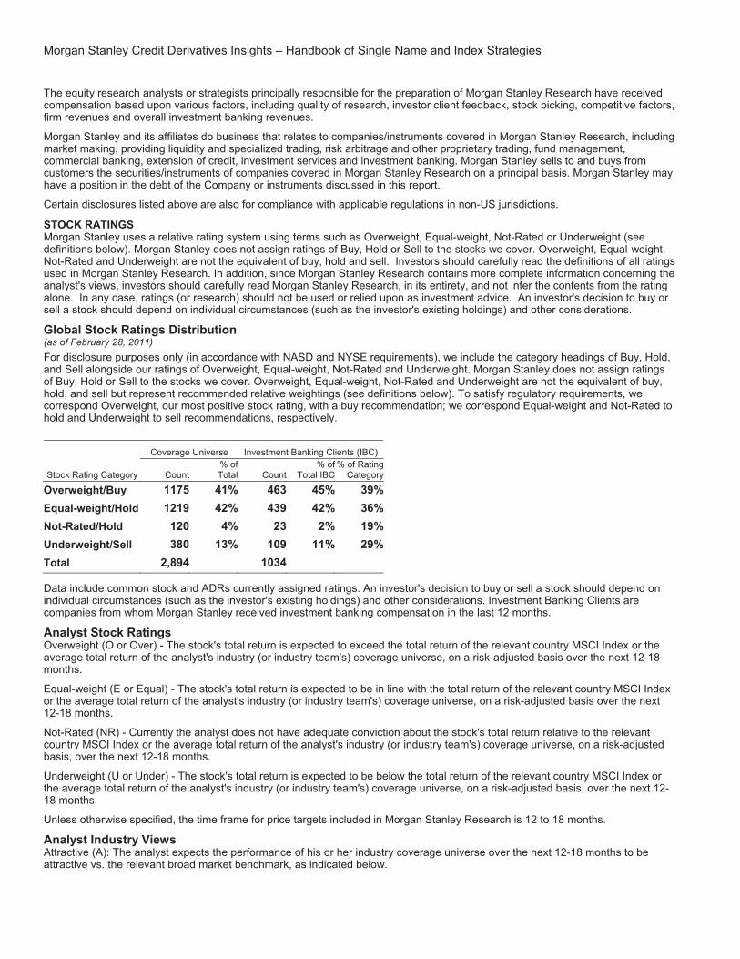
Morgan Stanley Credit Derivatives Insights – Handbook of Single Name and Index Strategies
The equity research analysts or strategists principally responsible for the preparation of Morgan Stanley Research have receivedcompensation based upon various factors, including quality of research, investor client feedback, stock picking, competitive factors,firm revenues and overall investment banking revenues.
Morgan Stanley and its affiliates do business that relates to companies/instruments covered in Morgan Stanley Research, including market making, providing liquidity and specialized trading, risk arbitrage and other proprietary trading, fund management, commercial banking, extension of credit, investment services and investment banking. Morgan Stanley sells to and buys from customers the securities/instruments of companies covered in Morgan Stanley Research on a principal basis. Morgan Stanley may have a position in the debt of the Company or instruments discussed in this report.
Certain disclosures listed above are also for compliance with applicable regulations in non-US jurisdictions.
STOCK RATINGS Morgan Stanley uses a relative rating system using terms such as Overweight, Equal-weight, Not-Rated or Underweight (see definitions below). Morgan Stanley does not assign ratings of Buy, Hold or Sell to the stocks we cover. Overweight, Equal-weight,Not-Rated and Underweight are not the equivalent of buy, hold and sell. Investors should carefully read the definitions of all ratings used in Morgan Stanley Research. In addition, since Morgan Stanley Research contains more complete information concerning the analyst's views, investors should carefully read Morgan Stanley Research, in its entirety, and not infer the contents from the ratingalone. In any case, ratings (or research) should not be used or relied upon as investment advice. An investor's decision to buy or sell a stock should depend on individual circumstances (such as the investor's existing holdings) and other considerations.
Global Stock Ratings Distribution (as of February 28, 2011) For disclosure purposes only (in accordance with NASD and NYSE requirements), we include the category headings of Buy, Hold, and Sell alongside our ratings of Overweight, Equal-weight, Not-Rated and Underweight. Morgan Stanley does not assign ratings of Buy, Hold or Sell to the stocks we cover. Overweight, Equal-weight, Not-Rated and Underweight are not the equivalent of buy,hold, and sell but represent recommended relative weightings (see definitions below). To satisfy regulatory requirements, we correspond Overweight, our most positive stock rating, with a buy recommendation; we correspond Equal-weight and Not-Rated to hold and Underweight to sell recommendations, respectively.
Coverage Universe Investment Banking Clients (IBC)
Stock Rating Category Count % ofTotal Count
% ofTotal IBC
% of Rating Category
Overweight/Buy 1175 41% 463 45% 39%Equal-weight/Hold 1219 42% 439 42% 36%Not-Rated/Hold 120 4% 23 2% 19%Underweight/Sell 380 13% 109 11% 29%Total 2,894 1034
Data include common stock and ADRs currently assigned ratings. An investor's decision to buy or sell a stock should depend on individual circumstances (such as the investor's existing holdings) and other considerations. Investment Banking Clients are companies from whom Morgan Stanley received investment banking compensation in the last 12 months.
Analyst Stock Ratings Overweight (O or Over) - The stock's total return is expected to exceed the total return of the relevant country MSCI Index or theaverage total return of the analyst's industry (or industry team's) coverage universe, on a risk-adjusted basis over the next 12-18months.
Equal-weight (E or Equal) - The stock's total return is expected to be in line with the total return of the relevant country MSCI Index or the average total return of the analyst's industry (or industry team's) coverage universe, on a risk-adjusted basis over the next 12-18 months.
Not-Rated (NR) - Currently the analyst does not have adequate conviction about the stock's total return relative to the relevantcountry MSCI Index or the average total return of the analyst's industry (or industry team's) coverage universe, on a risk-adjustedbasis, over the next 12-18 months.
Underweight (U or Under) - The stock's total return is expected to be below the total return of the relevant country MSCI Index or the average total return of the analyst's industry (or industry team's) coverage universe, on a risk-adjusted basis, over the next 12-18 months.
Unless otherwise specified, the time frame for price targets included in Morgan Stanley Research is 12 to 18 months.
Analyst Industry Views Attractive (A): The analyst expects the performance of his or her industry coverage universe over the next 12-18 months to be attractive vs. the relevant broad market benchmark, as indicated below.

In-Line (I): The analyst expects the performance of his or her industry coverage universe over the next 12-18 months to be in line with the relevant broad market benchmark, as indicated below.
Cautious (C): The analyst views the performance of his or her industry coverage universe over the next 12-18 months with cautionvs. the relevant broad market benchmark, as indicated below.
Benchmarks for each region are as follows: North America - S&P 500; Latin America - relevant MSCI country index or MSCI Latin America Index; Europe - MSCI Europe; Japan - TOPIX; Asia - relevant MSCI country index.
Important Disclosures for Morgan Stanley Smith Barney LLC Customers Citi Investment Research & Analysis (CIRA) research reports may be available about the companies or topics that are the subjectof Morgan Stanley Research. Ask your Financial Advisor or use Research Center to view any available CIRA research reports in addition to Morgan Stanley research reports.
Important disclosures regarding the relationship between the companies that are the subject of Morgan Stanley Research and Morgan Stanley Smith Barney LLC, Morgan Stanley and Citigroup Global Markets Inc. or any of their affiliates, are available on theMorgan Stanley Smith Barney disclosure website at www.morganstanleysmithbarney.com/researchdisclosures.
For Morgan Stanley and Citigroup Global Markets, Inc. specific disclosures, you may refer to www.morganstanley.com/researchdisclosures and https://www.citigroupgeo.com/geopublic/Disclosures/index_a.html.
Each Morgan Stanley Equity Research report is reviewed and approved on behalf of Morgan Stanley Smith Barney LLC. This review and approval is conducted by the same person who reviews the Equity Research report on behalf of Morgan Stanley. This could create a conflict of interest.
Other Important Disclosures Morgan Stanley & Co. International PLC and its affiliates have a significant financial interest in the debt securities of Assa Abloy AB, BSkyB, Bunge Ltd., Casino, Comcast Corporation, Cytec Industries Inc., Deutsche Telekom, DIRECTV, Freeport-McMoRan, International Paper, Johnson Controls, Inc., KPN, PPL Corporation, Safeway Inc., SES, Svenska Cellulosa AB, Telecom Italia, TheDow Chemical Company, Union Pacific Corp., Verizon Communications, Xerox Corp.
Morgan Stanley produces an equity research product called a "Tactical Idea." Views contained in a "Tactical Idea" on a particularstock may be contrary to the recommendations or views expressed in research on the same stock. This may be the result of differing time horizons, methodologies, market events, or other factors. For all research available on a particular stock, please contact your sales representative or go to Client Link at www.morganstanley.com.
Morgan Stanley Research does not provide individually tailored investment advice. Morgan Stanley Research has been prepared without regard to the individual financial circumstances and objectives of persons who receive it. Morgan Stanley recommends thatinvestors independently evaluate particular investments and strategies, and encourages investors to seek the advice of a financial adviser. The appropriateness of a particular investment or strategy will depend on an investor's individual circumstances and objectives. The securities, instruments, or strategies discussed in Morgan Stanley Research may not be suitable for all investors,and certain investors may not be eligible to purchase or participate in some or all of them.
The fixed income research analysts or strategists principally responsible for the preparation of Morgan Stanley Research have received compensation based upon various factors, including quality, accuracy and value of research, firm profitability or revenues (which include fixed income trading and capital markets profitability or revenues), client feedback and competitive factors. FixedIncome Research analysts' or strategists' compensation is not linked to investment banking or capital markets transactions performed by Morgan Stanley or the profitability or revenues of particular trading desks.
Morgan Stanley Research is not an offer to buy or sell or the solicitation of an offer to buy or sell any security/instrument or to participate in any particular trading strategy. The "Important US Regulatory Disclosures on Subject Companies" section in Morgan Stanley Research lists all companies mentioned where Morgan Stanley owns 1% or more of a class of common equity securities of the companies. For all other companies mentioned in Morgan Stanley Research, Morgan Stanley may have an investment of less than 1% in securities/instruments or derivatives of securities/instruments of companies and may trade them in ways different fromthose discussed in Morgan Stanley Research. Employees of Morgan Stanley not involved in the preparation of Morgan Stanley Research may have investments in securities/instruments or derivatives of securities/instruments of companies mentioned and may trade them in ways different from those discussed in Morgan Stanley Research. Derivatives may be issued by Morgan Stanley or associated persons.
With the exception of information regarding Morgan Stanley, Morgan Stanley Research is based on public information. Morgan Stanley makes every effort to use reliable, comprehensive information, but we make no representation that it is accurate or complete. We have no obligation to tell you when opinions or information in Morgan Stanley Research change apart from when we intend to discontinue equity research coverage of a subject company. Facts and views presented in Morgan Stanley Research have not been reviewed by, and may not reflect information known to, professionals in other Morgan Stanley business areas, including investment banking personnel.
Morgan Stanley Research personnel may participate in company events such as site visits and are generally prohibited from accepting payment by the company of associated expenses unless pre-approved by authorized members of Research management.

Morgan Stanley Credit Derivatives Insights – Handbook of Single Name and Index Strategies
The value of and income from your investments may vary because of changes in interest rates, foreign exchange rates, default rates, prepayment rates, securities/instruments prices, market indexes, operational or financial conditions of companies or otherfactors. There may be time limitations on the exercise of options or other rights in securities/instruments transactions. Past performance is not necessarily a guide to future performance. Estimates of future performance are based on assumptions that may not be realized. If provided, and unless otherwise stated, the closing price on the cover page is that of the primary exchange for the subject company's securities/instruments.
Morgan Stanley may make investment decisions or take proprietary positions that are inconsistent with the recommendations or views in this report.
To our readers in Taiwan: Information on securities/instruments that trade in Taiwan is distributed by Morgan Stanley Taiwan Limited ("MSTL"). Such information is for your reference only. Information on any securities/instruments issued by a company owned by the government of or incorporated in the PRC and listed in on the Stock Exchange of Hong Kong ("SEHK"), namely the H-shares, including the component company stocks of the Stock Exchange of Hong Kong ("SEHK")'s Hang Seng China Enterprise Index; or any securities/instruments issued by a company that is 30% or more directly- or indirectly-owned by the government of or a company incorporated in the PRC and traded on an exchange in Hong Kong or Macau, namely SEHK's Red Chip shares, including the component company of the SEHK's China-affiliated Corp Index is distributed only to Taiwan Securities Investment Trust Enterprises ("SITE"). The reader should independently evaluate the investment risks and is solely responsible for their investment decisions. Morgan Stanley Research may not be distributed to the public media or quoted or used by the public media without the express written consent of Morgan Stanley. Information on securities/instruments that do not trade in Taiwan is forinformational purposes only and is not to be construed as a recommendation or a solicitation to trade in such securities/instruments. MSTL may not execute transactions for clients in these securities/instruments.
To our readers in Hong Kong: Information is distributed in Hong Kong by and on behalf of, and is attributable to, Morgan StanleyAsia Limited as part of its regulated activities in Hong Kong. If you have any queries concerning Morgan Stanley Research, please contact our Hong Kong sales representatives.
Certain information in Morgan Stanley Research was sourced by employees of the Shanghai Representative Office of Morgan Stanley Asia Limited for the use of Morgan Stanley Asia Limited.
Morgan Stanley Research is disseminated in Japan by Morgan Stanley MUFG Securities Co., Ltd.; in Hong Kong by Morgan Stanley Asia Limited (which accepts responsibility for its contents); in Singapore by Morgan Stanley Asia (Singapore) Pte. (Registration number 199206298Z) and/or Morgan Stanley Asia (Singapore) Securities Pte Ltd (Registration number 200008434H), regulated by the Monetary Authority of Singapore, which accepts responsibility for its contents; in Australia to "wholesale clients" within the meaning of the Australian Corporations Act by Morgan Stanley Australia Limited A.B.N. 67 003 734576, holder of Australian financial services license No. 233742, which accepts responsibility for its contents; in Australia to"wholesale clients" and "retail clients" within the meaning of the Australian Corporations Act by Morgan Stanley Smith Barney Australia Pty Ltd (A.B.N. 19 009 145 555, holder of Australian financial services license No. 240813, which accepts responsibility for its contents; in Korea by Morgan Stanley & Co International plc, Seoul Branch; in India by Morgan Stanley India Company Private Limited; in Canada by Morgan Stanley Canada Limited, which has approved of, and has agreed to take responsibility for, the contents of Morgan Stanley Research in Canada; in Germany by Morgan Stanley Bank AG, Frankfurt am Main and Morgan Stanley Private Wealth Management Limited, Niederlassung Deutschland, regulated by Bundesanstalt fuer Finanzdienstleistungsaufsicht (BaFin); in Spain by Morgan Stanley, S.V., S.A., a Morgan Stanley group company, which is supervised by the Spanish Securities Markets Commission (CNMV) and states that Morgan Stanley Research has been written and distributed in accordance with the rules of conduct applicable to financial research as established under Spanish regulations;in the United States by Morgan Stanley & Co. Incorporated, which accepts responsibility for its contents. Morgan Stanley & Co.International plc, authorized and regulated by the Financial Services Authority, disseminates in the UK research that it has prepared, and approves solely for the purposes of section 21 of the Financial Services and Markets Act 2000, research which hasbeen prepared by any of its affiliates. Morgan Stanley Private Wealth Management Limited, authorized and regulated by the Financial Services Authority, also disseminates Morgan Stanley Research in the UK. Private U.K. investors should obtain the advice of their Morgan Stanley & Co. International plc or Morgan Stanley Private Wealth Management representative about the investments concerned. RMB Morgan Stanley (Proprietary) Limited is a member of the JSE Limited and regulated by the Financial Services Board in South Africa. RMB Morgan Stanley (Proprietary) Limited is a joint venture owned equally by Morgan Stanley International Holdings Inc. and RMB Investment Advisory (Proprietary) Limited, which is wholly owned by FirstRand Limited.
The information in Morgan Stanley Research is being communicated by Morgan Stanley & Co. International plc (DIFC Branch), regulated by the Dubai Financial Services Authority (the DFSA), and is directed at Professional Clients only, as defined by theDFSA. The financial products or financial services to which this research relates will only be made available to a customer who we are satisfied meets the regulatory criteria to be a Professional Client.
The information in Morgan Stanley Research is being communicated by Morgan Stanley & Co. International plc (QFC Branch), regulated by the Qatar Financial Centre Regulatory Authority (the QFCRA), and is directed at business customers and market counterparties only and is not intended for Retail Customers as defined by the QFCRA.
As required by the Capital Markets Board of Turkey, investment information, comments and recommendations stated here, are not within the scope of investment advisory activity. Investment advisory service is provided in accordance with a contract of engagement on investment advisory concluded between brokerage houses, portfolio management companies, non-deposit banks and clients. Comments and recommendations stated here rely on the individual opinions of the ones providing these comments

and recommendations. These opinions may not fit to your financial status, risk and return preferences. For this reason, to make an investment decision by relying solely to this information stated here may not bring about outcomes that fit your expectations.
The trademarks and service marks contained in Morgan Stanley Research are the property of their respective owners. Third-party data providers make no warranties or representations of any kind relating to the accuracy, completeness, or timeliness of the datathey provide and shall not have liability for any damages of any kind relating to such data. The Global Industry ClassificationStandard ("GICS") was developed by and is the exclusive property of MSCI and S&P.
Morgan Stanley has based its projections, opinions, forecasts and trading strategies regarding the MSCI Country Index Series solely on publicly available information. MSCI has not reviewed, approved or endorsed the projections, opinions, forecasts and trading strategies contained herein. Morgan Stanley has no influence on or control over MSCI's index compilation decisions.
Morgan Stanley Research, or any portion thereof may not be reprinted, sold or redistributed without the written consent of MorganStanley.
Morgan Stanley Research is disseminated and available primarily electronically, and, in some cases, in printed form. Additional information on recommended securities/instruments is available on request.

Morgan Stanley Credit Derivatives Insights – Handbook of Single Name and Index Strategies


www.morganstanley.com
NY C
S 66
26114 0
2/11
Sivan Mahadevan +1 (1) 212 761 1349 [email protected] Ashley Musfeldt +1 (1) 212 761 1727 [email protected] Phanikiran Naraparaju +44 (0) 207 677 5065 [email protected]
THE AMERICAS1585 Broadway New York, NY 10036-8293 United States Tel: +1 (1) 212 761 4000
EUROPE20 Bank Street, Canary Wharf London E14 4AD United Kingdom Tel: +44 (0) 20 7 425 8000
JAPAN4-20-3 Ebisu, Shibuya-ku Tokyo 150-6008 Japan Tel: +81 (0) 3 5424 -5000
ASIA /PACIFIC1 Austin Road West Kowloon Hong Kong Tel: +852 2848 5200
© 2011 Morgan Stanley