International Journal of Computer Vision 48(3), 215–231, 2002c© 2002 Kluwer Academic Publishers. Manufactured in The Netherlands.

Hamilton-Jacobi Skeletons

KALEEM SIDDIQI AND SYLVAIN BOUIXSchool of Computer Science & Center for Intelligent Machines, McGill University, Montreal,

QC H3A 2A7, Canadasiddiqi@cim.mcgill.ca

sbouix@cim.mcgill.ca

ALLEN TANNENBAUMDepartment of Electrical & Computer Engineering and Department of Biomedical Engineering,

Georgia Institute of Technology, Atlanta, GA 30082-0250, USAtannenba@ece.gatech.edu

STEVEN W. ZUCKERDepartments of Computer Science and Electrical Engineering and Center for Computational Vision & Control,

Yale University, New Haven, CT 06520-8285, USAzucker-steven@cs.yale.edu

Received June 30, 2000; Revised August 8, 2001; Accepted November 29, 2001

Abstract. The eikonal equation and variants of it are of significant interest for problems in computer vision andimage processing. It is the basis for continuous versions of mathematical morphology, stereo, shape-from-shadingand for recent dynamic theories of shape. Its numerical simulation can be delicate, owing to the formation ofsingularities in the evolving front and is typically based on level set methods. However, there are more classicalapproaches rooted in Hamiltonian physics which have yet to be widely used by the computer vision community. Inthis paper we review the Hamiltonian formulation, which offers specific advantages when it comes to the detectionof singularities or shocks. We specialize to the case of Blum’s grassfire flow and measure the average outwardflux of the vector field that underlies the Hamiltonian system. This measure has very different limiting behaviorsdepending upon whether the region over which it is computed shrinks to a singular point or a non-singular one.Hence, it is an effective way to distinguish between these two cases. We combine the flux measurement with ahomotopy preserving thinning process applied in a discrete lattice. This leads to a robust and accurate algorithmfor computing skeletons in 2D as well as 3D, which has low computational complexity. We illustrate the approachwith several computational examples.

Keywords: eikonal equation, Hamiltonian systems, flux and divergence, 2D and 3D skeletons, shape analysis

1. Introduction

Variational principles have emerged naturally fromconsiderations of energy minimization in mechanics(Lanczos, 1986). We consider these in the context of

the eikonal equation, which arises in geometrical opticsand has become of great interest for problems in com-puter vision (Bruss, 1989; Kimia et al., 1994). It isthe basis for continuous versions of mathematical mor-phology (Brockett and Maragos, 1992; Sapiro et al.,

216 Siddiqi et al.

1992; van den Boomgaard and Smeulders, 1994), aswell as for Blum’s grassfire transform (Blum, 1973)and dynamic theories of shape representation (Kimiaet al., 1995; Tari et al., 1997). It has also been usedfor applications in image processing and analysis(Sethian, 1996a; Caselles et al., 1998), shape-from-shading (Horn and Brooks, 1989; Rouy and Tourin,1992; Oliensis and Dupuis, 1994; Kimmel et al., 1995b)and stereo (Faugeras and Keriven, 1998).

As is well known, some care must be taken withthe numerical simulation of this equation, since it isa hyperbolic partial differential equation for which asmooth initial front may develop singularities or shocksas it propagates. At such points, classical concepts suchas the normal to a curve and its curvature are not de-fined. Nevertheless, it is precisely these points that areimportant for the above applications in computer vi-sion since, e.g., it is they which denote the skeleton(see Fig. 3.) To continue the evolution while preservingshocks, the technology of level set methods introducedby Osher and Sethian (1988) has proved to be extremelypowerful. The approach relies on the notion of a weaksolution, developed in viscosity theory (Crandall et al.,1992), and the introduction of an appropriate entropycondition to select it. The representation of the evolvingfront as a level set of a hypersurface allows topologicalchanges to be handled in a natural way and robust, ef-ficient implementations have recently been developed(Sethian, 1996b).

As pointed out by Osher and Sethian (1988), levelset methods are Eulerian in nature because compu-tations are restricted to grid points whose locationsare fixed. For such methods, the question of compu-ting the locus of shocks for dynamically changingsystems remains of crucial importance, i.e., the meth-ods are shock preserving but do not explicitly detectshocks. Shock detection methods which rely on inter-polation of the underlying hypersurface are compu-tationally very expensive. Numerical thresholds areintroduced, and high order accurate numerical schemesmust be used (Osher and Shu, 1991; Siddiqi et al.,1997).

On the other hand, there are more classical meth-ods rooted in Hamiltonian physics, which can alsobe used to study shock theory. Although such formu-lations have been applied to computer vision prob-lems (Horn and Brooks, 1989; Rouy and Tourin, 1992;Oliensis and Dupuis, 1994), the numerical methodshave yet to be widely used. In this paper we reviewthe Hamiltonian formalism for simulating the eikonal

equation which offers a number of conceptual advan-tages when it comes to shock tracking. Hamiltoniansystems are fundamental in classical physics and havea natural physical interpretation based on elementaryHamiltonian and Lagrangian mechanics. The existenceof such simple differential equations is also relevantto considering whether these models have any pos-sible biological implementations (Miller and Zucker,1999). We specialize to the case of Blum’s grassfireflow (Blum, 1973) and compute a measure of the av-erage outward flux of the vector field underlying theHamiltonian system. As the region over which thisflux is computed shrinks to a point, the measure canbe shown to have very different limiting behaviors de-pending upon whether or not that point is singular.Thus, it is a very effective way of distinguishing be-tween medial and non-medial points. We combine theaverage outward flux measure with a homotopy pre-serving thinning process applied in a discrete lattice.This leads to a robust and efficient algorithm for com-puting skeletons in 2D as well as 3D which has lowcomputational complexity. We illustrate the methodwith a number of examples of medial axes (2D) andmedial surfaces (3D) of synthetic objects as well ascomplex anatomical structures obtained from medicalimages.

To the best of our knowledge, the closest work incomputer vision is the formulation of Oliensis andDupuis of the shape-from-shading problem (Oliensisand Dupuis, 1994). Their method also uses Hamilton-Jacobi theory and has similar robust numerical prop-erties. In particular, a density function for markerparticles is propagated to obtain estimates of whereparticles accumulate. This strategy is used to distin-guish sources from sinks in order to reconstruct shapefrom intensity images. We now review some rele-vant background on skeletons, followed by a briefoverview of skeletonization approaches related to ourmethod.

1.1. 2D and 3D Skeletons

The 2D skeleton (medial axis) of a closed set A ⊂R2

is the locus of centers of maximal open discs containedwithin the complement of the set (Blum, 1973). Anopen disc is maximal if there exists no other opendisc contained in the complement of A that properlycontains the disc. The 3D skeleton (medial surface) of aclosed set A ⊂R3 is defined in an analogous fashion asthe locus of centers of maximal open spheres contained

Hamilton-Jacobi Skeletons 217

in the complement of the set. Both types of skeletonshave been widely used in bio-medicine for tasks in-volving object representation (Naf et al., 1996; Stettenand Pizer, 1999), registration (Liu et al., 1998a) andsegmentation (Sebastian et al., 1998). They have alsobeen used for graph-based object recognition in com-puter vision (Ogniewicz, 1993; Zhu and Yuille, 1996;Sharvit et al., 1998; Liu and Geiger, 1999; Siddiqi et al.,1999b), for animating objects in graphics (Teichmannand Teller, 1998; Pizer et al., 2001) and for manip-ulating them in computer-aided design. Despite theirpopularity, their numerical computation remains non-trivial. Most algorithms are not stable with respect tosmall perturbations of the boundary, and heuristic mea-sures for simplification are often introduced.

Interest in the skeleton as a representation for anobject stems from a number of interesting properties:(i) it is a thin set, i.e., it contains no interior points,(ii) it is homotopic to the original shape, (iii) it is in-variant under Euclidean transformations of the object(rotations and translations) and (iv) given the radiusof the maximal inscribed circle or sphere associatedwhich each skeletal point, the object can be recon-structed exactly. Hence, it provides a compact represen-tation while preserving the object’s genus and makingcertain useful properties explicit, such as its localwidth.

Approaches to computing skeletons can be broadlyorganized into three classes. First, methods based onthinning attempt to realize Blum’s grassfire formula-tion (Blum, 1973) by peeling away layers from an ob-ject while retaining special points (Arcelli and Sannitidi Baja, 1985; Lee and Kashyap, 1994; Borgefors et al.,1999; Manzanera et al., 1999). It is possible to defineerosion rules in a lattice such that the topology of theobject is preserved. However, these methods are quitesensitive to Euclidean transformations of the data andtypically fail to localize skeletal points accurately. Asa consequence, only a coarse approximation to the ob-ject is usually reconstructed (Manzanera et al., 1999;Bertrand, 1995; Lee and Kashyap, 1994).

Second, it has been shown that under appropriatesmoothness conditions the vertices of the Voronoi dia-gram of a set of boundary points converges to the exactskeleton as the sampling rate increases (Schmitt, 1989).This property has been exploited to develop skele-tonization algorithms in 2D (Ogniewicz, 1993), as wellas extensions to 3D (Sheehy et al., 1996; Sherbrookeet al., 1996). The dual of the Voronoi diagram, theDelaunay triangulation (or tetrahedralization in 3D)

has also been used extensively. Here the skeleton isdefined as the locus of centers of circumscribed cir-cles of each triangle (spheres of each tetrahedra in 3D)(Goldak et al., 1991; Naf et al., 1996). Both types ofmethods ensure homotopy between objects and theirskeletons and accurately localize skeletal points, pro-vided that the boundary is sampled densely. Unfortu-nately, the techniques used to prune elements of theVoronoi graph which correspond to small perturbationsof the boundary are typically based on heuristics. Inpractice, the results are not invariant under Euclideantransformations, and the optimization step, particularlyin 3D, can have a high computational complexity (Nafet al., 1996).

A third class of methods exploits the fact that thelocus of skeletal points coincides with the singulari-ties of a Euclidean distance function to the boundary.These approaches attempt to detect local maxima ofthe distance function, or the corresponding disconti-nuities in its derivatives (Arcelli and di Baja, 1992;Leymarie and Levine, 1992; Gomez and Faugeras,2000). The numerical detection of these singularities isitself a non-trivial problem; whereas it may be possibleto localize them, ensuring homotopy with the originalobject is difficult. The are also some recent approachesto computing 2D and 3D skeletons which combine as-pects of thinning, Voronoi diagrams and distance func-tions (Malandain and Fernandez-Vidal, 1998; Zhouet al., 1998; Borgefors et al., 1999; Tek and Kimia,1999).

1.2. Related Work

We now present a brief overview of selected approachesthat are related to the method we develop in this paper.We refrain from an exhaustive review of the large bodyof work in computer vision and computational geom-etry on computing 2D and 3D skeletons, since this isbeyond the scope of this paper.

Leymarie and Levine (1992) have simulated thegrassfire by utilizing the magnitude of the gradientvector field of a signed distance function to attract asnake moving in from the object’s boundary. In thistechnique the contour has to be first segmented at cur-vature extrema, which is itself a challenging problem.Kimmel et al. (1995a) have also proposed a methodwhere the contour is first segmented at locations ofpositive curvature maxima. Outward distance functionsto each segment are then computed and the skele-ton is obtained by interpolating the zero level set of

218 Siddiqi et al.

the distance map differences and removing spuriouspoints. Liu et al. (1998b) have introduced a varia-tional approach to computing symmetric axis trees,where portions of a curve are matched against others,incorporating constraints including co-circularity andparallelism. The approach leads to an abstraction that isrelated to the medial axis but is comprised by a differ-ent locus of points. Dynamic programming is used tomake the computation efficient. Tek and Kimia (1999)have proposed an approach for calculating symmetrymaps, which is based on the combination of a wave-front propagation technique with an exact (analytic)distance function. In this technique the representationmust be pruned in order to distinguish salient branchesfrom unwanted ones. Pudney (1998) has introduced adistance ordered homotopy preserving thinning proce-dure where points are removed in order of their distancefrom the boundary while anchoring end points and cen-ters of maximal balls identified from a chamfer distancefunction. Malandain and Fernandez-Vidal (1998) ob-tain two sets based on thresholding a function of twoheuristic measures, φ and d , to characterize the sin-gularities of the Euclidean distance function. The twosets are combined using a topological reconstructionprocess. Tari and Shah (1998) have proposed a charac-terization of the symmetries of n-dimensional shapesby looking at properties of the Hessian of a suitably de-fined scalar edge-strength functional. Furst and Pizer(1998) have introduced a notion of an optimal param-eter height ridge in arbitrary dimension by exploitinga sub-dimensional maximum property. Kalitzin et al.(1998) have considered index computations on vectorfields associated with scalar images in order to iden-tify their singularities. Vector fields rooted in magneto-statics have also been used for extracting symmetry andedge lines in greyscale images (Cross and Hancock,1997).

2. The Eikonal Equation

We begin by showing the connection between a mono-tonically advancing front and the well known eikonalequation. Consider the curve evolution equation

∂C∂t

= FN , (1)

where C is the vector of curve coordinates, N is theunit inward normal and F = F(x, y) is the speed ofthe front at each point in the plane, with F ≥ 0 (the

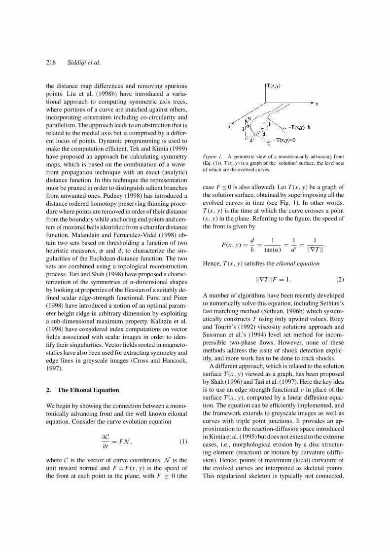
Figure 1. A geometric view of a monotonically advancing front(Eq. (1)). T (x, y) is a graph of the ‘solution’ surface, the level setsof which are the evolved curves.

case F ≤ 0 is also allowed). Let T (x, y) be a graph ofthe solution surface, obtained by superimposing all theevolved curves in time (see Fig. 1). In other words,T (x, y) is the time at which the curve crosses a point(x, y) in the plane. Referring to the figure, the speed ofthe front is given by

F(x, y) = d

h= 1

tan(α)= 1

d ′ = 1

‖∇T ‖ .

Hence, T (x, y) satisfies the eikonal equation

‖∇T ‖F = 1. (2)

A number of algorithms have been recently developedto numerically solve this equation, including Sethian’sfast marching method (Sethian, 1996b) which system-atically constructs T using only upwind values, Rouyand Tourin’s (1992) viscosity solutions approach andSussman et al.’s (1994) level set method for incom-pressible two-phase flows. However, none of thesemethods address the issue of shock detection explic-itly, and more work has to be done to track shocks.

A different approach, which is related to the solutionsurface T (x, y) viewed as a graph, has been proposedby Shah (1996) and Tari et al. (1997). Here the key ideais to use an edge strength functional v in place of thesurface T (x, y), computed by a linear diffusion equa-tion. The equation can be efficiently implemented, andthe framework extends to greyscale images as well ascurves with triple point junctions. It provides an ap-proximation to the reaction-diffusion space introducedin Kimia et al. (1995) but does not extend to the extremecases, i.e., morphological erosion by a disc structur-ing element (reaction) or motion by curvature (diffu-sion). Hence, points of maximum (local) curvature ofthe evolved curves are interpreted as skeletal points.This regularized skeleton is typically not connected,

Hamilton-Jacobi Skeletons 219

and its relation to the classical skeleton, obtained fromthe eikonal equation with F = 1, is as yet unclear.

In the next section, we shall consider an alternateframework for solving the eikonal equation, which isbased on the canonical equations of Hamilton. Thetechnique is widely used in classical mechanics andrests on the use of a Legendre transformation (seeArnold (1989) and Shankar (1994)), which takes asystem of n second-order differential equations to amathematically equivalent system of 2n first-order dif-ferential equations. We believe that the method offersspecific advantages over alternatives for a numberof vision problems that involve shock tracking andskeletonization.

3. Hamilton’s Canonical Equationsand the Hamilton-Jacobi Skeleton Flow

We begin this section with an overview of theHamiltonian formalism, taken from Arnold (1989) andShankar (1994). Although this is standard material inclassical mechanics, these techniques may be unfa-miliar to the general computer vision audience. In aLagrangian formulation the independent variables arethe coordinates q of particles and their velocities q.For example, in the context of the Eq. (1) these wouldbe the positions of points along the curve C and theirassociated velocities FN . Each particle follows thepath of least action in reaching a future location at afuture time. In mathematical terms, the action functionminimized, Sq0,t0 , is given by

Sq0,t0 (q, t) =∫

γ

L dt.

Here γ is an extremal curve connecting the points(q0, t0) and (q, t) and L(q, q) is the Lagrangian. Inother words, of all possible paths connecting (q0, t0)and (q, t), the trajectory γ followed by the particleis the one that minimizes the action function. Theassociated Euler-Lagrange equation is

d

dt

∂L∂q

− ∂L∂q

= 0 (3)

where the momenta are derived quantities given by

p = ∂L∂q

.

The key to the Hamiltonian formalism is to exchangethe roles of q and p by replacing the LagrangianL(q, q)with a HamiltonianH(q, p) such that the velocities nowbecome the derived quantities

q = ∂H∂p

.

This can be done by applying the following Legendretransformation:

H(q, p) = p · q − L(q, q) (4)

where the q′s are written as functions of q’s and p’s. Itis a simple exercise to verify that the above expressionfor the velocities q then holds. One can also take partialderivatives of the Hamiltonian with respect to the q’sand verify that

∂H∂q

= −∂L∂q

.

Using Eq. (3), ∂L∂q can be replaced with p to give

Hamilton’s canonical equations:

p = −∂H∂q

, q = ∂H∂p

. (5)

Thus, in the Hamiltonian formalism one starts withthe initial positions and momenta (q(0), p(0)) and in-tegrates Eq. (5) to obtain the phase space (q(t), p(t))of the system. A comparison of the Lagrangian andHamiltonian formalisms is presented in Table 1.

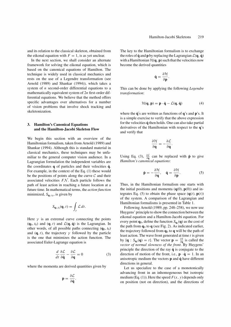
Following Arnold (1989, pp. 248–258), we now useHuygens’ principle to show the connection between theeikonal equation and a Hamilton-Jacobi equation. Forevery point q0, define the function Sq0 (q) as the cost ofthe path from q0 to q (see Fig. 2). As indicated earlier,the trajectory followed from q0 to q will be the path ofleast action. The wave front generated at time t is givenby {q : Sq0 (q) = t}. The vector p = ∂S

∂q is called thevector of normal slowness of the front. By Huygens’principle the direction of the ray q is conjugate to thedirection of motion of the front, i.e., p · q = 1. In ananisotropic medium the vectors p and q have differentdirections in general.

Let us specialize to the case of a monotonicallyadvancing front in an inhomogeneous but isotropicmedium (Eq. (1)). Here the speed F(x, y) depends onlyon position (not on direction), and the directions of

220 Siddiqi et al.

Table 1. A comparison of the Lagrangian and Hamiltonian formalisms, taken from Shankar (1994).

The Lagrangian formalism The Hamiltonian formalism

The state of the system is described by (q, q). The state of the system is described by (q, p).

The state may be represented by a point moving with avelocity in an n-dimensional configuration space.

The state may be represented by a point in a2n-dimensional phase space.

The n coordinates evolve according to n second-orderequations.

The 2n coordinates and momenta obey 2nfirst-order equations.

For a given L several trajectories may pass through agiven point in the configuration space.

For a given H only one trajectory passesthrough a given point in the phase space.

Figure 2. Direction of a ray q and the direction of motion of thewave front p. From Arnold (1989).

p and q coincide. The Lagrangian associated with theaction function minimized (Eq. (3)) is given by

L = 1

F(x, y)‖∂γ /∂t‖ = 1

F(x, y)‖q‖.

This can be interpreted as a conformal (infinitesimal)length element, and we have assumed that the extremalsemanating from the point (q0, t0) do not intersect else-where, i.e., they form a central field of extremals. For anisotropic medium the extremals turn out to be straightlines, and for the special case F(x, y) = −1 the actionfunction becomes Euclidean length.

It can be shown that the vector of normal slowness,p = ∂S

∂q , is not arbitrary but satisfies the Hamilton-Jacobi equation

∂S

∂t= −H

(q,

∂S

∂q

), (6)

where the Hamiltonian function H(q, p) is theLegendre transformation with respect to q of theLagrangian discussed earlier (Arnold, 1989). Ratherthan solve the nonlinear Hamilton-Jacobi equation forthe action function S (which will give the solution sur-face T (x, y) to Eq. (2)), it is much more convenient tolook at the evolution of the phase space (q(t), p(t))

under the equivalent Hamiltonian system given byEq. (5). This offers a number of advantages, the mostsignificant being that the equations become linear andhence trivial to simulate numerically. We shall now de-rive this system of equations for the special case of afront advancing with speed F(x, y) = 1. This case isof particular interest for shape analysis because the lo-cus of shocks which from coincides with the trace ofthe Blum skeleton (Blum, 1973; Brockett and Maragos,1992; Kimia et al., 1995).

For the case of a front moving with constant speed,recall that the action function being minimized isEuclidean length and hence S can be viewed as aEuclidean distance function from the initial curve C0.Furthermore, the magnitude of its gradient, ‖∇S‖, isidentical to 1 in its smooth regime, which is preciselywhere the assumption of a central field of extremals isvalid.

With q = (x, y), p = (Sx , Sy), ‖p‖ = 1, we asso-ciate to the evolving plane curve C ⊂ R2 the surfaceC ⊂ R4 given by

C : = {(x, y, Sx , Sy) : (x, y)

∈ C, S2x + S2

y = 1, p · q = 1}.

The Hamiltonian function obtained by applying theLegendre transformation (Eq. (4)) to the LagrangianL = −‖q‖ is given by

H = p · q − L = 1 + (S2

x + S2y

) 12 .

The associated Hamiltonian system is

p = −∂H∂q

= (0, 0), q = ∂H∂p

= (Sx , Sy).

(7)

C can be evolved under this system of equations, withC(t) ⊂ R4 denoting the resulting (contact) surface. The

Hamilton-Jacobi Skeletons 221

projection of C(t) onto R2 will then give the parallelevolution of C at time t, C(t).

We illustrate this flow by representing the initialcurve with a sequence of marker particles and thenevolving them according to Eq. (7). Further detailsare presented in Siddiqi et al. (1999a). With q =(x, y), p = (Sx , Sy) = ∇S, the system of equationsbecomes

{Sx = 0, Sy = 0; x = Sx , y = Sy},

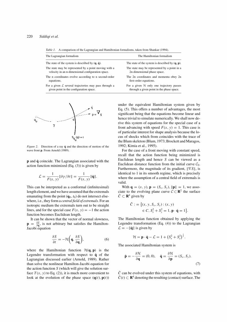
a gradient dynamical system. The second equation in-dicates that the trajectory of the marker particles willbe governed by the vector field obtained from the gra-dient of the Euclidean distance function S, and the firstindicates that this vector field does not change withtime and can be computed once at the beginning of thesimulation. Projecting this 4D system onto the (x, y)plane for each instance of time t will give the evolvedcurve C(t). The superposition of all the level curvesgives the solution surface T (x, y) in Fig. 1. Figure 3depicts the evolution of marker particles, with speedF = 1, for several different shapes.

Whereas a variety of methods can be used to simu-late the eikonal equation, including level set techniques

Figure 3. The evolution of marker particles under the Hamiltoniansystem. The initial particles are placed on the boundary and iterationsof the process are superimposed. These correspond to level sets ofthe solution surface T (x, y) in Fig. 1.

and their fast marching versions (Sethian, 1996b), theHamiltonian formalism offers the advantage that thecomputed flow is less sensitive to boundary details.Furthermore, the formation of shocks can be made ex-plicit. As shown in the following section the key ideais to exploit a measure of the average outward flux ofthe vector field q.

4. Flux and Divergence

We approach the discrimination of medial points,which coincide with the shocks of the grassfire flow,from non-medial ones, by computing the average out-ward flux of the vector field q about a point. The averageoutward flux is defined as the outward flux through theboundary of a region containing the point, normalizedby the length of the boundary

∫δR〈q,N 〉 ds

length(δR)(8)

Here ds is an element of the bounding contour δR ofthe region R and N is the outward normal at each pointof the contour. Via the divergence theorem

∫R

div(q)da ≡∫

δR〈q,N 〉 ds, (9)

where da is an area element. Thus the outward flux isrelated to the divergence in the following way

div(q) ≡ lim�a→0

∫δR〈q,N 〉 ds

�a. (10)

The outward flux, or equivalently the integral of thedivergence of q, measures the degree to which the flowgenerated by q is area preserving for the region overwhich it is computed. To elaborate, the outward flux(and hence also the average outward flux) is negativeif the area enclosed by the region δR is shrinking un-der the action of the Hamiltonian flow, positive if it isgrowing and zero otherwise. This quantity is clearlystrongly dependent on the shape of the region R. How-ever, it can be shown that in the limit as the region δRshrinks to a non-medial point, the average outward fluxapproaches zero independent of the shape of R.

When considering a region δR that contains a me-dial point, unfortunately the standard form of the di-vergence theorem does not apply since the vector fieldq becomes singular. Instead, the limiting behavior ofthe average outward flux as the region δR shrinks to a

222 Siddiqi et al.

medial point can be considered. Furthermore, it can beshown that there is a constant cR > 0 depending on theshape of the region R such that the average outward fluxappoaches a strictly negative number bounded aboveby cR × 〈q,N ′〉, where N ′ is now a one-sided normalto the medial axis or surface.1 This constant coversall the cases of a regular axis point, a branch point,or an end point. Thus, in the limit as δR shrinks to apoint the average outward flux calculation is an effec-tive way of detecting the singularities of the vector fieldq. Non-medial points give values that are close to zeroand medial points corresponding to strong singularitiesgive large negative values. Whereas thus far we havefocused on the case of a (2D) closed curve, the verysame analysis applies to a closed (3D) surface evolv-ing according to an eikonal equation. One simply has toreplace the initial closed curveC with the closed surfaceS in Eq. (1), add a third coordinate z to the phase spacein Eq. (7) and replace the area element with a volume el-ement and the contour integral with a surface integral inEqs. (8)–(10).

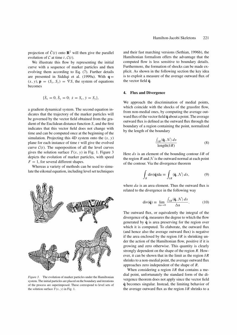
Figure 4 illustrates the average outward flux com-putation on the silhouette of a panther shape, wherevalues close to zero are shown in medium grey. Allcomputations are carried out on a rectangular lattice,although the bounding curve is shown in interpolatedform. Strictly speaking, the average outward flux is de-sired only in the limit as the region shrinks to a point.However, the average outward flux over a very smallneighborhood (a circle in 2D or a sphere in 3D) providesa sufficient approximation to the limiting values. Strongsingularities correspond either to high magnitude neg-ative (dark grey) or positive numbers (light grey), de-pending upon whether the vector field is collapsingat or emanating from a particular point. A thresholdon the average outward flux yields a close approxima-tion to the skeleton, as used in Siddiqi et al. (1999a).

Figure 4. The gradient vector field of a signed distance function tothe boundary of a panther shape (left), with the associated averageoutward flux (right). Whereas the smooth regime of the vector fieldgives zero flux (medium grey), strong singularities give either largenegative values (dark grey) in the interior or large positive values(light grey) in the exterior.

Figure 5. Thresholding the average outward flux map in Fig. 4. Ahigh threshold yields a connected set, but it is not thin and unwantedbranches are present (left). A low threshold yields a closer approxi-mation to the desired medial axis, but the result is now disconnected(right).

However, in general it is impossible to guarantee thatthe result obtained by simple thresholding is homo-topic to the original shape. A high threshold may yielda connected set, but it is not thin and unwanted branchesmay be present, Fig. 5 (left). A low threshold yields athin set, but it may be disconnected, Fig. 5 (right). Thesolution, as we shall now show, is to introduce addi-tional constraints to ensure that the resulting skeleton ishomotopic to the shape. The essential idea is to incor-porate a homotopy preserving thinning process, wherethe removal of points is guided by the average outwardflux values. In the context of the Hamilton-Jacobi skele-ton flow (Eq. (7)), this leads to a robust and efficientalgorithm for computing 2D and 3D skeletons.

5. Homotopy Preserving Skeletons

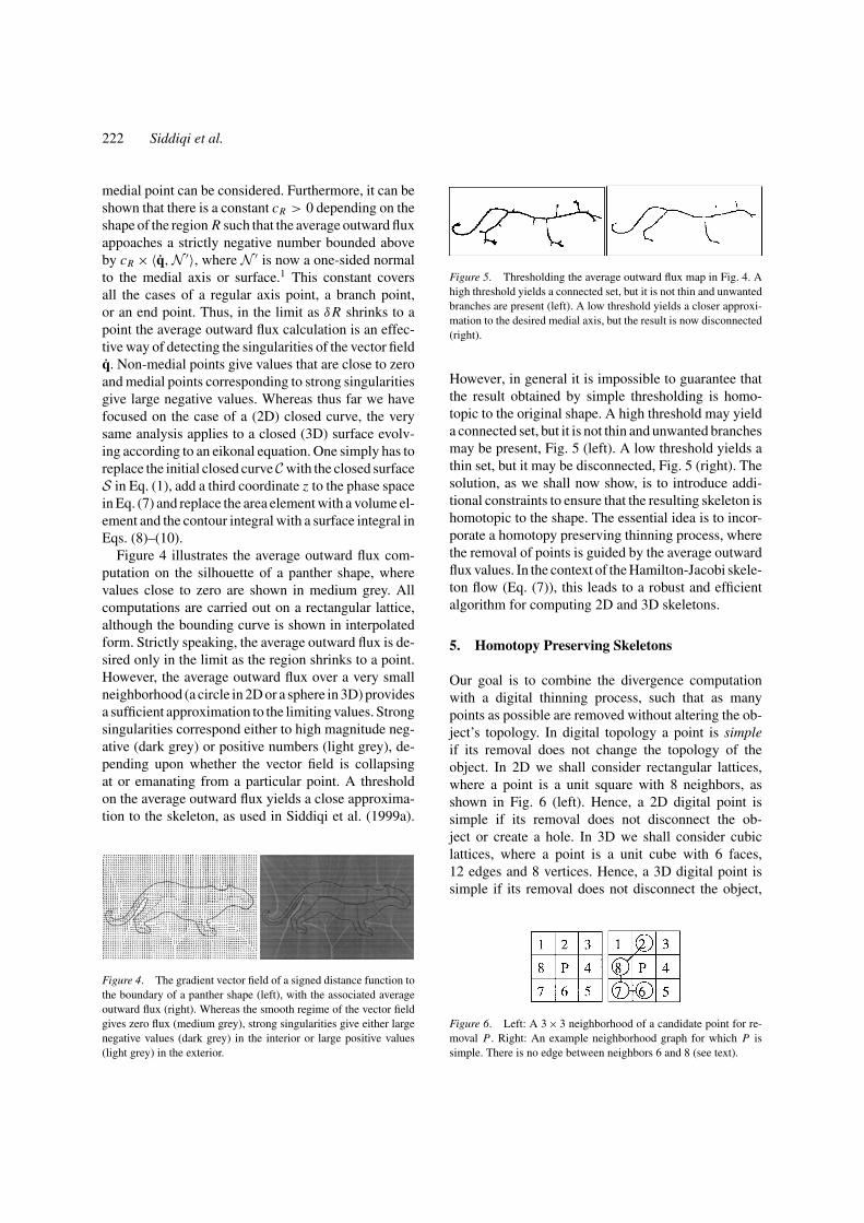
Our goal is to combine the divergence computationwith a digital thinning process, such that as manypoints as possible are removed without altering the ob-ject’s topology. In digital topology a point is simpleif its removal does not change the topology of theobject. In 2D we shall consider rectangular lattices,where a point is a unit square with 8 neighbors, asshown in Fig. 6 (left). Hence, a 2D digital point issimple if its removal does not disconnect the ob-ject or create a hole. In 3D we shall consider cubiclattices, where a point is a unit cube with 6 faces,12 edges and 8 vertices. Hence, a 3D digital point issimple if its removal does not disconnect the object,

Figure 6. Left: A 3 × 3 neighborhood of a candidate point for re-moval P . Right: An example neighborhood graph for which P issimple. There is no edge between neighbors 6 and 8 (see text).

Hamilton-Jacobi Skeletons 223

create a hole, or create a cavity (Kong and Rosenfeld,1989).

5.1. 2D Simple Points

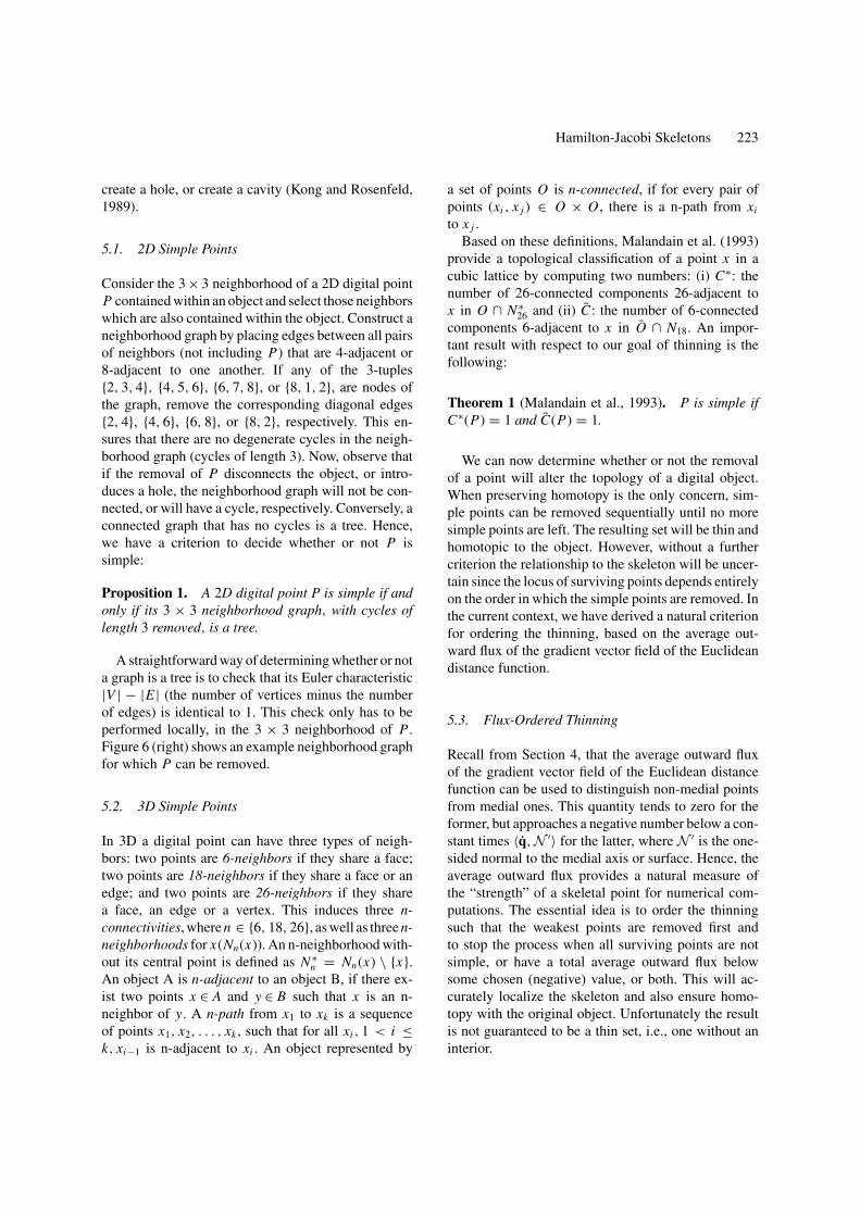
Consider the 3 × 3 neighborhood of a 2D digital pointP contained within an object and select those neighborswhich are also contained within the object. Construct aneighborhood graph by placing edges between all pairsof neighbors (not including P) that are 4-adjacent or8-adjacent to one another. If any of the 3-tuples{2, 3, 4}, {4, 5, 6}, {6, 7, 8}, or {8, 1, 2}, are nodes ofthe graph, remove the corresponding diagonal edges{2, 4}, {4, 6}, {6, 8}, or {8, 2}, respectively. This en-sures that there are no degenerate cycles in the neigh-borhood graph (cycles of length 3). Now, observe thatif the removal of P disconnects the object, or intro-duces a hole, the neighborhood graph will not be con-nected, or will have a cycle, respectively. Conversely, aconnected graph that has no cycles is a tree. Hence,we have a criterion to decide whether or not P issimple:

Proposition 1. A 2D digital point P is simple if andonly if its 3 × 3 neighborhood graph, with cycles oflength 3 removed, is a tree.

A straightforward way of determining whether or nota graph is a tree is to check that its Euler characteristic|V | − |E | (the number of vertices minus the numberof edges) is identical to 1. This check only has to beperformed locally, in the 3 × 3 neighborhood of P .Figure 6 (right) shows an example neighborhood graphfor which P can be removed.

5.2. 3D Simple Points

In 3D a digital point can have three types of neigh-bors: two points are 6-neighbors if they share a face;two points are 18-neighbors if they share a face or anedge; and two points are 26-neighbors if they sharea face, an edge or a vertex. This induces three n-connectivities, where n ∈ {6, 18, 26}, as well as three n-neighborhoods for x(Nn(x)). An n-neighborhood with-out its central point is defined as N ∗

n = Nn(x) \ {x}.An object A is n-adjacent to an object B, if there ex-ist two points x ∈ A and y ∈ B such that x is an n-neighbor of y. A n-path from x1 to xk is a sequenceof points x1, x2, . . . , xk , such that for all xi , 1 < i ≤k, xi−1 is n-adjacent to xi . An object represented by

a set of points O is n-connected, if for every pair ofpoints (xi , x j ) ∈ O × O , there is a n-path from xi

to x j .Based on these definitions, Malandain et al. (1993)

provide a topological classification of a point x in acubic lattice by computing two numbers: (i) C∗: thenumber of 26-connected components 26-adjacent tox in O ∩ N ∗

26 and (ii) C : the number of 6-connectedcomponents 6-adjacent to x in O ∩ N18. An impor-tant result with respect to our goal of thinning is thefollowing:

Theorem 1 (Malandain et al., 1993). P is simple ifC∗(P) = 1 and C(P) = 1.

We can now determine whether or not the removalof a point will alter the topology of a digital object.When preserving homotopy is the only concern, sim-ple points can be removed sequentially until no moresimple points are left. The resulting set will be thin andhomotopic to the object. However, without a furthercriterion the relationship to the skeleton will be uncer-tain since the locus of surviving points depends entirelyon the order in which the simple points are removed. Inthe current context, we have derived a natural criterionfor ordering the thinning, based on the average out-ward flux of the gradient vector field of the Euclideandistance function.

5.3. Flux-Ordered Thinning

Recall from Section 4, that the average outward fluxof the gradient vector field of the Euclidean distancefunction can be used to distinguish non-medial pointsfrom medial ones. This quantity tends to zero for theformer, but approaches a negative number below a con-stant times 〈q,N ′〉 for the latter, where N ′ is the one-sided normal to the medial axis or surface. Hence, theaverage outward flux provides a natural measure ofthe “strength” of a skeletal point for numerical com-putations. The essential idea is to order the thinningsuch that the weakest points are removed first andto stop the process when all surviving points are notsimple, or have a total average outward flux belowsome chosen (negative) value, or both. This will ac-curately localize the skeleton and also ensure homo-topy with the original object. Unfortunately the resultis not guaranteed to be a thin set, i.e., one without aninterior.

224 Siddiqi et al.

One way of satisfying this last constraint is to de-fine an appropriate notion of an end point. Such a pointwould correspond to the end point of a curve (in 2D or3D), or a point on the rim of a surface, in 3D. The thin-ning process would proceed as before, but the thresh-old criterion for removal would be applied only to endpoints. Hence, all surviving points which were not endpoints would not be simple and the result would be athin set.

In 2D, an end point will be viewed as any point thatcould be the end of a 4-connected or 8-connected digitalcurve. It is straightforward to see that such a point maybe characterized as follows:

Proposition 2. A 2D point P could be an endpoint of a 1 pixel thick digital curve if, in a 3 × 3neighborhood, it has a single neighbor, or it hastwo neighbors, both of which are 4-adjacent to oneanother.

In 3D, the characterization of an end point is moredifficult. An end point is either the end of a 26-connected curve, or a corner or point on the rim of a26-connected surface. In R3, if there exists a plane thatpasses through a point p such that the intersection ofthe plane with the object includes an open curve whichends at p, then p is an end point of a 3D curve, or ison the rim or corner of a 3D surface. This criterion canbe discretized easily to 26-connected digital objects byexamining 9 digital planes in the 26-neighborhood ofp as in Pudney (1998).

5.4. The Algorithm and its Complexity

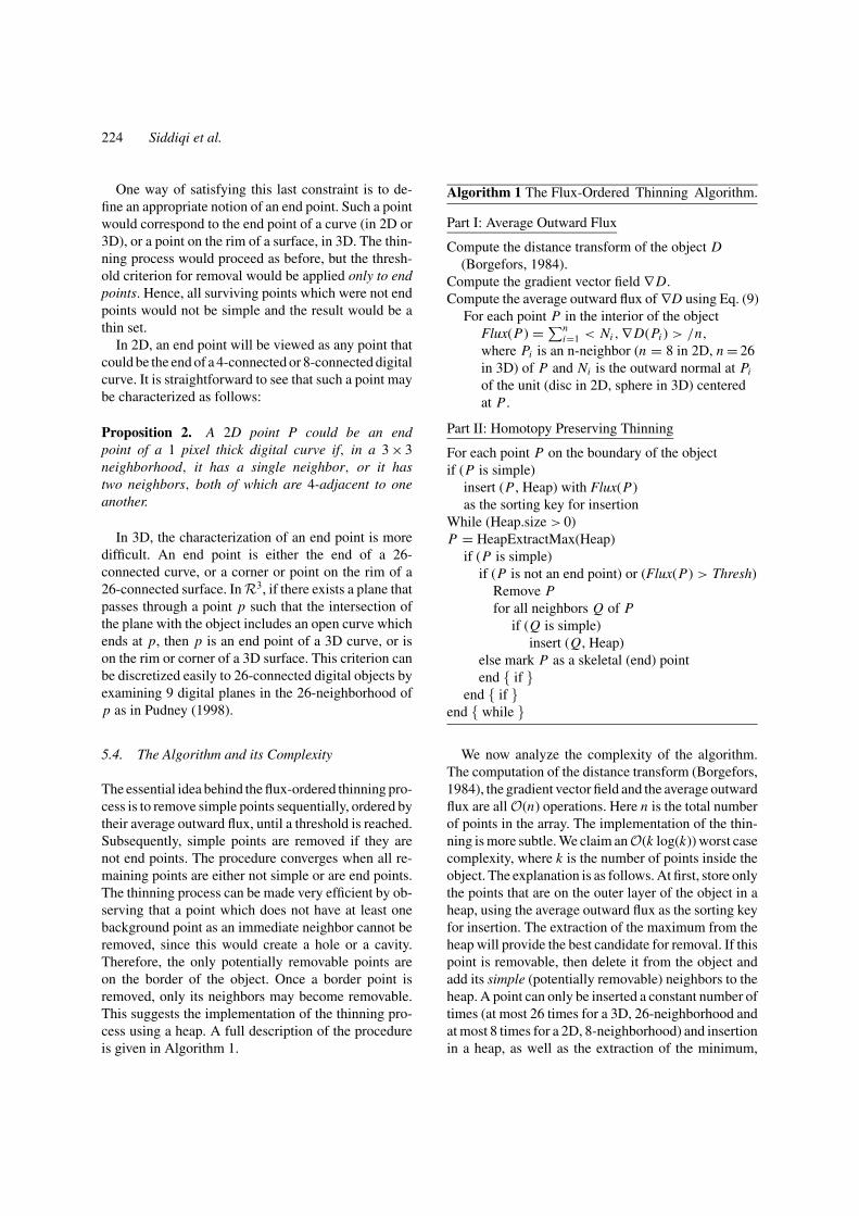
The essential idea behind the flux-ordered thinning pro-cess is to remove simple points sequentially, ordered bytheir average outward flux, until a threshold is reached.Subsequently, simple points are removed if they arenot end points. The procedure converges when all re-maining points are either not simple or are end points.The thinning process can be made very efficient by ob-serving that a point which does not have at least onebackground point as an immediate neighbor cannot beremoved, since this would create a hole or a cavity.Therefore, the only potentially removable points areon the border of the object. Once a border point isremoved, only its neighbors may become removable.This suggests the implementation of the thinning pro-cess using a heap. A full description of the procedureis given in Algorithm 1.

Algorithm 1 The Flux-Ordered Thinning Algorithm.

Part I: Average Outward Flux

Compute the distance transform of the object D(Borgefors, 1984).

Compute the gradient vector field ∇ D.Compute the average outward flux of ∇D using Eq. (9)

For each point P in the interior of the objectFlux(P) = ∑n

i=1 < Ni , ∇ D(Pi ) > /n,

where Pi is an n-neighbor (n = 8 in 2D, n = 26in 3D) of P and Ni is the outward normal at Pi

of the unit (disc in 2D, sphere in 3D) centeredat P .

Part II: Homotopy Preserving Thinning

For each point P on the boundary of the objectif (P is simple)

insert (P , Heap) with Flux(P)as the sorting key for insertion

While (Heap.size > 0)P = HeapExtractMax(Heap)

if (P is simple)if (P is not an end point) or (Flux(P) > Thresh)

Remove Pfor all neighbors Q of P

if (Q is simple)insert (Q, Heap)

else mark P as a skeletal (end) pointend { if }

end { if }end { while }

We now analyze the complexity of the algorithm.The computation of the distance transform (Borgefors,1984), the gradient vector field and the average outwardflux are all O(n) operations. Here n is the total numberof points in the array. The implementation of the thin-ning is more subtle. We claim anO(k log(k)) worst casecomplexity, where k is the number of points inside theobject. The explanation is as follows. At first, store onlythe points that are on the outer layer of the object in aheap, using the average outward flux as the sorting keyfor insertion. The extraction of the maximum from theheap will provide the best candidate for removal. If thispoint is removable, then delete it from the object andadd its simple (potentially removable) neighbors to theheap. A point can only be inserted a constant number oftimes (at most 26 times for a 3D, 26-neighborhood andat most 8 times for a 2D, 8-neighborhood) and insertionin a heap, as well as the extraction of the minimum,

Hamilton-Jacobi Skeletons 225

are both O(log(l)) operations, where l is the numberof elements in the heap. There cannot be more than kelements in the heap, because we only have a total of kpoints within the object. The worst case complexity forthinning is thereforeO(k log(k)). Hence, the worst casecomplexity of the algorithm is O(n)+ O(k log(k)). Weshould point out that this is a very loose upper bound.The heap only contains points from the object’s sur-face and therefore in practice the complexity is almostlinear in the number of digital points n.

6. Examples

6.1. Medial Axes

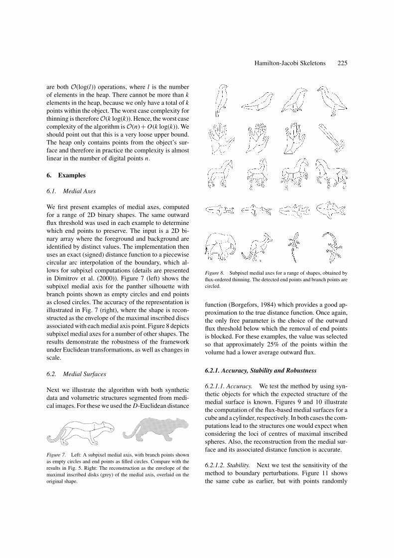
We first present examples of medial axes, computedfor a range of 2D binary shapes. The same outwardflux threshold was used in each example to determinewhich end points to preserve. The input is a 2D bi-nary array where the foreground and background areidentified by distinct values. The implementation thenuses an exact (signed) distance function to a piecewisecircular arc interpolation of the boundary, which al-lows for subpixel computations (details are presentedin Dimitrov et al. (2000)). Figure 7 (left) shows thesubpixel medial axis for the panther silhouette withbranch points shown as empty circles and end pointsas closed circles. The accuracy of the representation isillustrated in Fig. 7 (right), where the shape is recon-structed as the envelope of the maximal inscribed discsassociated with each medial axis point. Figure 8 depictssubpixel medial axes for a number of other shapes. Theresults demonstrate the robustness of the frameworkunder Euclidean transformations, as well as changes inscale.

6.2. Medial Surfaces

Next we illustrate the algorithm with both syntheticdata and volumetric structures segmented from medi-cal images. For these we used the D-Euclidean distance

Figure 7. Left: A subpixel medial axis, with branch points shownas empty circles and end points as filled circles. Compare with theresults in Fig. 5. Right: The reconstruction as the envelope of themaximal inscribed disks (grey) of the medial axis, overlaid on theoriginal shape.

Figure 8. Subpixel medial axes for a range of shapes, obtained byflux-ordered thinning. The detected end points and branch points arecircled.

function (Borgefors, 1984) which provides a good ap-proximation to the true distance function. Once again,the only free parameter is the choice of the outwardflux threshold below which the removal of end pointsis blocked. For these examples, the value was selectedso that approximately 25% of the points within thevolume had a lower average outward flux.

6.2.1. Accuracy, Stability and Robustness

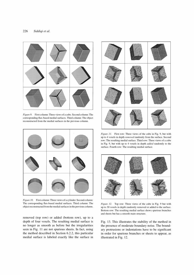
6.2.1.1. Accuracy. We test the method by using syn-thetic objects for which the expected structure of themedial surface is known. Figures 9 and 10 illustratethe computation of the flux-based medial surfaces for acube and a cylinder, respectively. In both cases the com-putations lead to the structures one would expect whenconsidering the loci of centres of maximal inscribedspheres. Also, the reconstruction from the medial sur-face and its associated distance function is accurate.

6.2.1.2. Stability. Next we test the sensitivity of themethod to boundary perturbations. Figure 11 showsthe same cube as earlier, but with points randomly

226 Siddiqi et al.

Figure 9. First column: Three views of a cube. Second column: Thecorresponding flux-based medial surfaces. Third column: The objectreconstructed from the medial surfaces in the previous column.

Figure 10. First column: Three views of a cylinder. Second column:The corresponding flux-based medial surfaces. Third column: Theobject reconstructed from the medial surfaces in the previous column.

removed (top row) or added (bottom row), up to adepth of four voxels. The resulting medial surface isno longer as smooth as before but the irregularitiesseen in Fig. 11 are not spurious sheets. In fact, usingthe method described in Section 6.2.2, this particularmedial surface is labeled exactly like the surface in

Figure 11. First row: Three views of the cube in Fig. 9, but withup to 4 voxels in depth removed randomly from the surface. Secondrow: The resulting medial surface. Third row: Three views of a cubein Fig. 9, but with up to 4 voxels in depth added randomly to thesurface. Fourth row: The resulting medial surface.

Figure 12. Top row: Three views of the cube in Fig. 9 but withup to 30 voxels in depth randomly removed or added to the surface.Bottom row: The resulting medial surface shows spurious branchesand sheets but has a smooth main structure.

Fig. 13. This illustrates the stability of the method inthe presence of moderate boundary noise. The bound-ary protrusions or indentations have to be significantin order for spurious branches or sheets to appear, asillustrated in Fig. 12.

Hamilton-Jacobi Skeletons 227

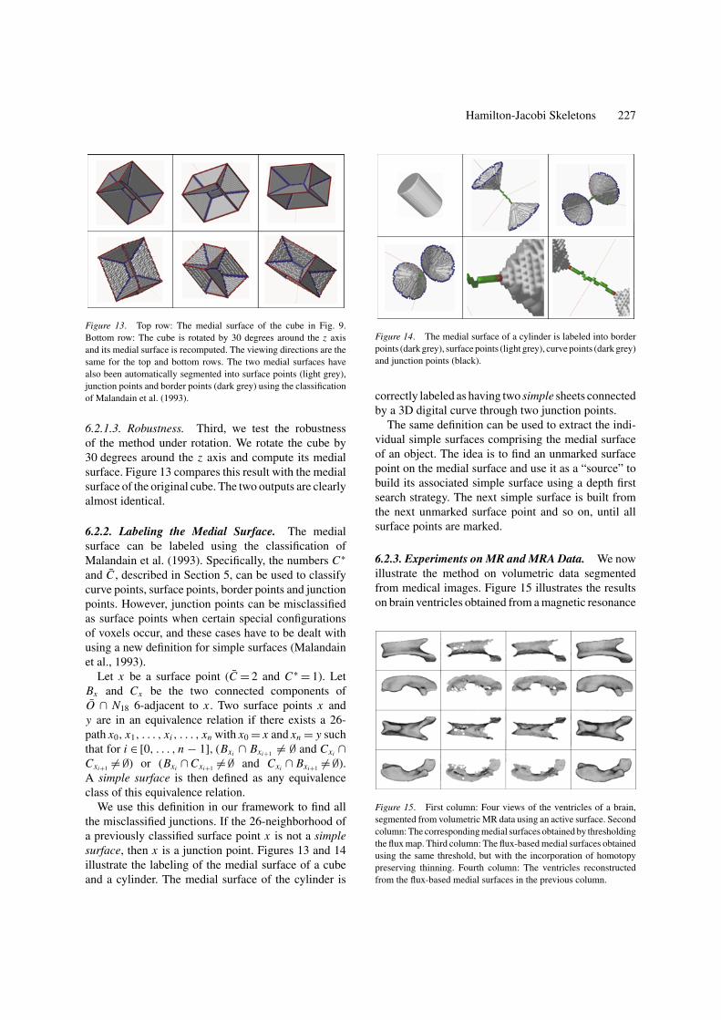
Figure 13. Top row: The medial surface of the cube in Fig. 9.Bottom row: The cube is rotated by 30 degrees around the z axisand its medial surface is recomputed. The viewing directions are thesame for the top and bottom rows. The two medial surfaces havealso been automatically segmented into surface points (light grey),junction points and border points (dark grey) using the classificationof Malandain et al. (1993).

6.2.1.3. Robustness. Third, we test the robustnessof the method under rotation. We rotate the cube by30 degrees around the z axis and compute its medialsurface. Figure 13 compares this result with the medialsurface of the original cube. The two outputs are clearlyalmost identical.

6.2.2. Labeling the Medial Surface. The medialsurface can be labeled using the classification ofMalandain et al. (1993). Specifically, the numbers C∗

and C , described in Section 5, can be used to classifycurve points, surface points, border points and junctionpoints. However, junction points can be misclassifiedas surface points when certain special configurationsof voxels occur, and these cases have to be dealt withusing a new definition for simple surfaces (Malandainet al., 1993).

Let x be a surface point (C = 2 and C∗ = 1). LetBx and Cx be the two connected components ofO ∩ N18 6-adjacent to x . Two surface points x andy are in an equivalence relation if there exists a 26-path x0, x1, . . . , xi , . . . , xn with x0 = x and xn = y suchthat for i ∈ [0, . . . , n − 1], (Bxi ∩ Bxi+1 �= ∅ and Cxi ∩Cxi+1 �= ∅) or (Bxi ∩ Cxi+1 �= ∅ and Cxi ∩ Bxi+1 �= ∅).A simple surface is then defined as any equivalenceclass of this equivalence relation.

We use this definition in our framework to find allthe misclassified junctions. If the 26-neighborhood ofa previously classified surface point x is not a simplesurface, then x is a junction point. Figures 13 and 14illustrate the labeling of the medial surface of a cubeand a cylinder. The medial surface of the cylinder is

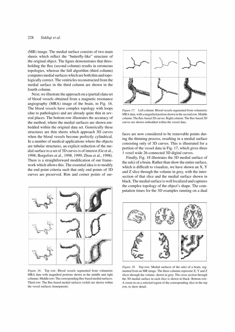
Figure 14. The medial surface of a cylinder is labeled into borderpoints (dark grey), surface points (light grey), curve points (dark grey)and junction points (black).

correctly labeled as having two simple sheets connectedby a 3D digital curve through two junction points.

The same definition can be used to extract the indi-vidual simple surfaces comprising the medial surfaceof an object. The idea is to find an unmarked surfacepoint on the medial surface and use it as a “source” tobuild its associated simple surface using a depth firstsearch strategy. The next simple surface is built fromthe next unmarked surface point and so on, until allsurface points are marked.

6.2.3. Experiments on MR and MRA Data. We nowillustrate the method on volumetric data segmentedfrom medical images. Figure 15 illustrates the resultson brain ventricles obtained from a magnetic resonance

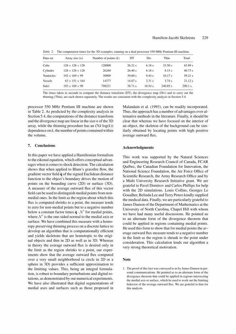
Figure 15. First column: Four views of the ventricles of a brain,segmented from volumetric MR data using an active surface. Secondcolumn: The corresponding medial surfaces obtained by thresholdingthe flux map. Third column: The flux-based medial surfaces obtainedusing the same threshold, but with the incorporation of homotopypreserving thinning. Fourth column: The ventricles reconstructedfrom the flux-based medial surfaces in the previous column.

228 Siddiqi et al.

(MR) image. The medial surface consists of two mainsheets which reflect the “butterfly-like” structure ofthe original object. The figure demonstrates that thres-holding the flux (second column) results in erroneoustopologies, whereas the full algorithm (third column)computes medial surfaces which are both thin and topo-logically correct. The ventricles reconstructed from themedial surface in the third column are shown in thefourth column.

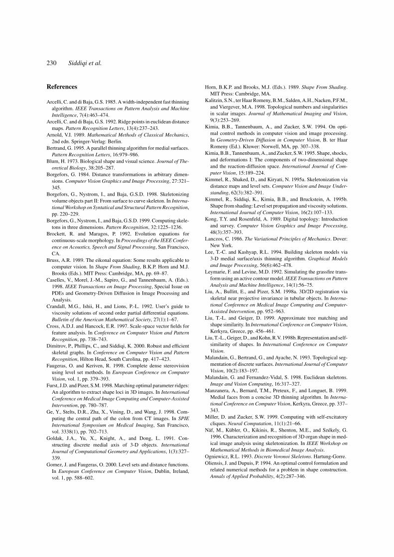
Next, we illustrate the approach on a (partial) data setof blood vessels obtained from a magnetic resonanceangiography (MRA) image of the brain, in Fig. 16.The blood vessels have complex topology with loops(due to pathologies) and are already quite thin in sev-eral places. The bottom row illustrates the accuracy ofthe method, where the medial surfaces are shown em-bedded within the original data set. Generically thesestructures are thin sheets which approach 3D curveswhen the blood vessels become perfectly cylindrical.In a number of medical applications where the objectsare tubular structures, an explicit reduction of the me-dial surface to a set of 3D curves is of interest (Ge et al.,1998; Borgefors et al., 1998, 1999; Zhou et al., 1998).There is a straightforward modification of our frame-work which allows this. The essential idea is to modifythe end point criteria such that only end points of 3Dcurves are preserved. Rim and corner points of sur-

Figure 16. Top row: Blood vessels segmented from volumetricMRA data with magnified portions shown in the middle and rightcolumns. Middle row: The corresponding flux-based medial surfaces.Third row: The flux-based medial surfaces (solid) are shown withinthe vessel surfaces (transparent).

Figure 17. Left column: Blood vessels segmented from volumetricMRA data, with a magnified portion shown in the second row. Middlecolumn: The flux-based 3D curves. Right column: The flux-based 3Dcurves are shown embedded within the vessel data.

faces are now considered to be removable points dur-ing the thinning process, resulting in a medial surfaceconsisting only of 3D curves. This is illustrated for aportion of the vessel data in Fig. 17, which gives three1 voxel wide 26-connected 3D digital curves.

Finally, Fig. 18 illustrates the 3D medial surface ofthe sulci of a brain. Rather than show the entire surface,which is difficult to visualize, we have shown an X, Yand Z slice through the volume in grey, with the inter-section of that slice and the medial surface shown inblack. The medial surface is well localized and capturesthe complex topology of the object’s shape. The com-putation times for the 3D examples running on a dual

Figure 18. Top row: Medial surfaces of the sulci of a brain, seg-mented from an MR image. The three columns represent X, Y and Zslices through the volume, shown in grey. The cross section throughthe 3D medial surface in each slice is shown in black. Bottom row:A zoom-in on a selected region of the corresponding slice in the toprow, to show detail.

Hamilton-Jacobi Skeletons 229

Table 2. The computation times for the 3D examples, running on a dual processor 550 MHz Pentium III machine.

Data set Array size (n) Number of points (k) DT Div Thin Total

Cube 128 × 128 × 128 120000 26.21 s 6.18 s 33.50 s 65.89 s

Cylinder 128 × 128 × 128 26260 26.40 s 6.18 s 8.15 s 40.73 s

Ventricles 192 × 169 × 99 30909 39.60 s 9.44 s 10.17 s 59.21 s

Vessels 63 × 151 × 164 14377 14.07 s 3.31 s 3.74 s 21.12 s

Sulci 192 × 169 × 99 798221 38.71 s 10.54 s 240.85 s 290.1 s

The times taken in seconds to compute the distance transform (DT), the divergence map (Div) and to carry out thethinning (Thin), are each shown separately. The results are consistent with the complexity analysis in Section 5.4.

processor 550 MHz Pentium III machine are shownin Table 2. As predicted by the complexity analysis inSection 5.4, the computations of the distance transformand the divergence map are linear in the size n of the 3Darray, while the thinning procedure has an O(k log(k))dependence on k, the number of points contained withinthe volume.

7. Conclusions

In this paper we have applied a Hamiltonian formalismto the eikonal equation, which offers conceptual advan-tages when it comes to shock detection. The calculationshows that when applied to Blum’s grassfire flow, thegradient vector field q of the signed Euclidean distancefunction to the object’s boundary drives the motion ofpoints on the bounding curve (2D) or surface (3D).A measure of the average outward flux of this vectorfield can be used to distinguish medial points from non-medial ones. In the limit as the region about which thisflux is computed shrinks to a point, the measure tendsto zero for non-medial points but to a negative numberbelow a constant factor times q ·N ′ for medial points,where N ′ is the one-sided normal to the medial axis orsurface. We have combined this measure with a homo-topy preserving thinning process on a discrete lattice todevelop an algorithm that is computationally efficientand yields skeletons that are homotopic to the origi-nal objects and thin in 2D as well as in 3D. Whereasin theory the average outward flux is desired only inthe limit as the region shrinks to a point, our exper-iments show that the average outward flux computedover a very small neighborhood (a circle in 2D or asphere in 3D) provides a sufficient approximation tothe limiting values. This, being an integral formula-tion, is robust to boundary perturbations and digital ro-tations, as demonstrated by our numerical experiments.We have also illustrated that digital segmentations ofmedial axes and surfaces such as those proposed in

Malandain et al. (1993), can be readily incorporated.Thus, the approach has a number of advantages over al-ternative methods in the literature. Finally, it should beclear that whereas we have focused on the interior ofan object, the skeleton of the background can be sim-ilarly obtained by locating points with high positiveaverage outward flux.

Acknowledgments

This work was supported by the Natural Sciencesand Engineering Research Council of Canada, FCARQuebec, the Canadian Foundation for Innovation, theNational Science Foundation, the Air Force Office ofScientific Research, the Army Research Office and bya Multi University Research Initiative grant. We aregrateful to Pavel Dimitrov and Carlos Phillips for helpwith the 2D simulations. Louis Collins, Georges LeGoualher, Belinda Lee and Terry Peters kindly suppliedthe medical data. Finally, we are particularly grateful toJames Damon of the Department of Mathematics at theUniversity of North Carolina, Chapel Hill with whomwe have had many useful discussions. He pointed usto an alternate form of the divergence theorem thatcould be applied in regions containing medial points.He used this form to show that for medial points the av-erage outward flux measure tends to a negative numberin the limit as the region is shrunk to the point underconsideration. This calculation lends our algorithm avery strong theoretical motivation.

Note

1. The proof of this fact was conveyed to us by James Damon in per-sonal communications. He pointed us to an alternate form of thedivergence theorem that could be applied in regions intersectingthe medial axis or surface, which he used to work out the limitingbehavior of the average outward flux. We are grateful to him forthis analysis.

230 Siddiqi et al.

References

Arcelli, C. and di Baja, G.S. 1985. A width-independent fast thinningalgorithm. IEEE Transactions on Pattern Analysis and MachineIntelligence, 7(4):463–474.

Arcelli, C. and di Baja, G.S. 1992. Ridge points in euclidean distancemaps. Pattern Recognition Letters, 13(4):237–243.

Arnold, V.I. 1989. Mathematical Methods of Classical Mechanics,2nd edn. Springer-Verlag: Berlin.

Bertrand, G. 1995. A parallel thinning algorithm for medial surfaces.Pattern Recognition Letters, 16:979–986.

Blum, H. 1973. Biological shape and visual science. Journal of The-oretical Biology, 38:205–287.

Borgefors, G. 1984. Distance transformations in arbitrary dimen-sions. Computer Vision Graphics and Image Processing, 27:321–345.

Borgefors, G., Nystrom, I., and Baja, G.S.D. 1998. Skeletonizingvolume objects part II: From surface to curve skeleton. In Interna-tional Workshop on Syntatical and Structural Pattern Recognition,pp. 220–229.

Borgefors, G., Nystrom, I., and Baja, G.S.D. 1999. Computing skele-tons in three dimensions. Pattern Recognition, 32:1225–1236.

Brockett, R. and Maragos, P. 1992. Evolution equations forcontinuous-scale morphology. In Proceedings of the IEEE Confer-ence on Acoustics, Speech and Signal Processing, San Francisco,CA.

Bruss, A.R. 1989. The eikonal equation: Some results applicable tocomputer vision. In Shape From Shading, B.K.P. Horn and M.J.Brooks (Eds.). MIT Press: Cambridge, MA, pp. 69–87.

Caselles, V., Morel, J.-M., Sapiro, G., and Tannenbaum, A. (Eds.).1998. IEEE Transactions on Image Processing, Special Issue onPDEs and Geometry-Driven Diffusion in Image Processing andAnalysis.

Crandall, M.G., Ishii, H., and Lions, P.-L. 1992. User’s guide toviscosity solutions of second order partial differential equations.Bulletin of the American Mathematical Society, 27(1):1–67.

Cross, A.D.J. and Hancock, E.R. 1997. Scale-space vector fields forfeature analysis. In Conference on Computer Vision and PatternRecognition, pp. 738–743.

Dimitrov, P., Phillips, C., and Siddiqi, K. 2000. Robust and efficientskeletal graphs. In Conference on Computer Vision and PatternRecognition, Hilton Head, South Carolina, pp. 417–423.

Faugeras, O. and Keriven, R. 1998. Complete dense stereovisionusing level set methods. In European Conference on ComputerVision, vol. 1, pp. 379–393.

Furst, J.D. and Pizer, S.M. 1998. Marching optimal parameter ridges:An algorithm to extract shape loci in 3D images. In InternationalConference on Medical Image Computing and Computer-AssistedIntervention, pp. 780–787.

Ge, Y., Stelts, D.R., Zha, X., Vining, D., and Wang, J. 1998. Com-puting the central path of the colon from CT images. In SPIEInternational Symposium on Medical Imaging, San Francisco,vol. 3338(1), pp. 702–713.

Goldak, J.A., Yu, X., Knight, A., and Dong, L. 1991. Con-structing discrete medial axis of 3-D objects. InternationalJournal of Computational Geometry and Applications, 1(3):327–339.

Gomez, J. and Faugeras, O. 2000. Level sets and distance functions.In European Conference on Computer Vision, Dublin, Ireland,vol. 1, pp. 588–602.

Horn, B.K.P. and Brooks, M.J. (Eds.). 1989. Shape From Shading.MIT Press: Cambridge, MA.

Kalitzin, S.N., ter Haar Romeny, B.M., Salden, A.H., Nacken, P.F.M.,and Viergever, M.A. 1998. Topological numbers and singularitiesin scalar images. Journal of Mathematical Imaging and Vision,9(3):253–269.

Kimia, B.B., Tannenbaum, A., and Zucker, S.W. 1994. On opti-mal control methods in computer vision and image processing.In Geometry-Driven Diffusion in Computer Vision, B. ter HaarRomeny (Ed.). Kluwer: Norwell, MA, pp. 307–338.

Kimia, B.B., Tannenbaum, A., and Zucker, S.W. 1995. Shape, shocks,and deformations I: The components of two-dimensional shapeand the reaction-diffusion space. International Journal of Com-puter Vision, 15:189–224.

Kimmel, R., Shaked, D., and Kiryati, N. 1995a. Skeletonization viadistance maps and level sets. Computer Vision and Image Under-standing, 62(3):382–391.

Kimmel, R., Siddiqi, K., Kimia, B.B., and Bruckstein, A. 1995b.Shape from shading: Level set propagation and viscosity solutions.International Journal of Computer Vision, 16(2):107–133.

Kong, T.Y. and Rosenfeld, A. 1989. Digital topology: Introductionand survey. Computer Vision Graphics and Image Processing,48(3):357–393.

Lanczos, C. 1986. The Variational Principles of Mechanics. Dover:New York.

Lee, T.-C. and Kashyap, R.L. 1994. Building skeleton models via3-D medial surface/axis thinning algorithm. Graphical Modelsand Image Processing, 56(6):462–478.

Leymarie, F. and Levine, M.D. 1992. Simulating the grassfire trans-form using an active contour model. IEEE Transactions on PatternAnalysis and Machine Intelligence, 14(1):56–75.

Liu, A., Bullitt, E., and Pizer, S.M. 1998a. 3D/2D registration viaskeletal near projective invariance in tubular objects. In Interna-tional Conference on Medical Image Computing and Computer-Assisted Intervention, pp. 952–963.

Liu, T.-L. and Geiger, D. 1999. Approximate tree matching andshape similarity. In International Conference on Computer Vision,Kerkyra, Greece, pp. 456–461.

Liu, T.-L., Geiger, D., and Kohn, R.V. 1998b. Representation and self-similarity of shapes. In International Conference on ComputerVision.

Malandain, G., Bertrand, G., and Ayache, N. 1993. Topological seg-mentation of discrete surfaces. International Journal of ComputerVision, 10(2):183–197.

Malandain, G. and Fernandez-Vidal, S. 1998. Euclidean skeletons.Image and Vision Computing, 16:317–327.

Manzanera, A., Bernard, T.M., Preteux, F., and Longuet, B. 1999.Medial faces from a concise 3D thinning algorithm. In Interna-tional Conference on Computer Vision, Kerkyra, Greece, pp. 337–343.

Miller, D. and Zucker, S.W. 1999. Computing with self-excitatorycliques. Neural Computation, 11(1):21–66.

Naf, M., Kubler, O., Kikinis, R., Shenton, M.E., and Szekely, G.1996. Characterization and recognition of 3D organ shape in med-ical image analysis using skeletonization. In IEEE Workshop onMathematical Methods in Biomedical Image Analysis.

Ogniewicz, R.L. 1993. Discrete Voronoi Skeletons. Hartung-Gorre.Oliensis, J. and Dupuis, P. 1994. An optimal control formulation and

related numerical methods for a problem in shape construction.Annals of Applied Probability, 4(2):287–346.

Hamilton-Jacobi Skeletons 231

Osher, S. and Shu, C.-W. 1991. High-order essentially non-oscillatory schemes for Hamilton-Jacobi equations. SIAM Journalof Numerical Analysis, 28:907–922.

Osher, S.J. and Sethian, J.A. 1988. Fronts propagating with cur-vature dependent speed: Algorithms based on Hamilton-Jacobiformulations. Journal of Computational Physics, 79:12–49.

Pizer, S.M., Joshi, S., Fletcher, P., Styner, M., Tracton, G., and Chen,Z. 2001. Segmentation of single-figure objects by deformableM-reps. In Medical Image Computing and Computer-Assisted In-tervention, W.J. Niessen and M.A. Viergever (Eds.). vol. 2208 ofLecture Notes in Computer Science. Springer: Berlin, pp. 862–871.

Pudney, C. 1998. Distance-ordered homotopic thinning: A skele-tonization algorithm for 3D digital images. Computer Vision andImage Understanding, 72(3):404–413.

Rouy, E. and Tourin, A. 1992. A viscosity solutions approachto shape-from-shading. SIAM Journal of Numerical Analysis,29(3):867–884.

Sapiro, G., Kimia, B.B., Kimmel, R., Shaked, D., and Bruckstein,A. 1992. Implementing continuous-scale morphology. PatternRecognition, 26(9).

Schmitt, M. 1989. Some examples of algorithms analysis in compu-tational geometry by means of mathematical morphology tech-niques. In Lecture Notes in Computer Science, Geometry andRobotics, vol. 391, J. Boissonnat and J. Laumond (Eds.). Springer-Verlag: Berlin, pp. 225–246.

Sebastian, T.B., Tek, H., Crisco, J.J., Wolfe, S.W., and Kimia, B.B.1998. Segmentation of carpal bones from 3D CT images usingskeletally coupled deformable models. In International Confer-ence on Medical Image Computing and Computer-Assisted Inter-vention, pp. 1184–1194.

Sethian, J. 1996a. Level Set Methods: Evolving Interfaces in Geom-etry, Fluid Mechanics, Computer Vision, and Materials Science.Cambridge University Press: Cambridge.

Sethian, J.A. 1996b. A fast marching level set method for monoton-ically advancing fronts. In Proceedings of the National Academyof Sciences, USA, 93:1591–1595.

Shah, J. 1996. A common framework for curve evolution, segmenta-tion and anisotropic diffusion. In Conference on Computer Visionand Pattern Recognition, pp. 136–142.

Shankar, R. 1994. Principles of Quantum Mechanics. Plenum Press:New York.

Sharvit, D., Chan, J., Tek, H., and Kimia, B.B. 1998. Symmetry-based indexing of image databases. In IEEE Workshop on Content-Based Access of Image and Video Libraries.

Sheehy, D.J., Armstrong, C.G., and Robinson, D.J. 1996. Shape

description by medial surface construction. IEEE Transactionson Visualization and Computer Graphics, 2(1):62–72.

Sherbrooke, E.C., Patrikalakis, N., and Brisson, E. 1996. An algo-rithm for the medial axis transform of 3D polyhedral solids. IEEETransactions on Visualization and Computer Graphics, 2(1):44–61.

Siddiqi, K., Bouix, S., Tannenbaum, A., and Zucker, S.W. 1999a.The Hamilton-Jacobi Skeleton. In International Conference onComputer Vision, Kerkyra, Greece, pp. 828–834.

Siddiqi, K., Kimia, B.B., and Shu, C. 1997. Geometric shock-capturing eno schemes for subpixel interpolation, computationand curve evolution. Graphical Models and Image Processing,59(5):278–301.

Siddiqi, K., Shokoufandeh, A., Dickinson, S.J., and Zucker, S.W.1999b. Shock graphs and shape matching. International Journalof Computer Vision, 35(1):13–32.

Stetten, G.D., and Pizer, S.M. 1999. Automated identification andmeasurement of objects via populations of medial primitives,with application to real time 3D echocardiography. In Interna-tional Conference on Information Processing in Medical Imaging,pp. 84–97.

Sussman, M., Smereka, P., and Osher, S. 1994. A level set approachfor computing solutions to incompressible two-phase flow. Journalof Computational Physics, 114:146–154.

Tari, S. and Shah, J. 1998. Local symmetries of shapes in arbi-trary dimension. In International Conference on Computer Vision,Bombay, India.

Tari, Z.S.G., Shah, J., and Pien, H. 1997. Extraction of shape skele-tons from grayscale images. Computer Vision and Image Under-standing, 66:133–146.

Teichmann, M. and Teller, S. 1998. Assisted articulation of closedpolygonal models. In 9th Eurographics Workshop on Animationand Simulation.

Tek, H. and Kimia, B.B. 1999. Symmetry maps of free-form curvesegments via wave propagation. In International Conference onComputer Vision, Kerkyra, Greece, pp. 362–369.

van den Boomgaard, R. and Smeulders, A. 1994. The morphologicalstructure of images: The differential equations of morphologicalscale-space. IEEE Transactions on Pattern Analysis and Machineintelligence, 16(11):1101–1113.

Zhou, Y., Kaufman, A., and Toga, A.W. 1998. 3D skeleton and center-line generation based on an approximate minimum distance field.International Journal of the Visual Computer, 14(7):303–314.

Zhu, S. and Yuille, A.L. 1996. FORMS: A flexible object recognitionand modeling system. International Journal of Computer Vision,20(3):187–212.