halocarbon ozone depletion and global warming potentials · chapter 4 n92-15434 halocarbon ozone...
TRANSCRIPT
chapter 4
N92-15434
HALOCARBON OZONEDEPLETION AND
GLOBAL WARMING POTENTIALS
Coordinators
R. A. Cox (UK) and D. Wuebbles (USA)
Principal Authors and Contributors
R. Atkinson (Australia)
P. Connell (USA)
R. A. Cox (UK)
H. P. Dorn (FRG)
A. De Rudder (Belgium)
R. G. Derwent (UK)
F. C. Fehsenfeld (USA)
D. Fisher (USA)
I. Isaksen (Norway)
M. Ko (USA)
R. Lesclaux (France)
S. C. Liu (USA)
S. A. Penkett (UK)
V. Ramaswamy (USA)
J. Rudolph (FRG)
H. B. Singh (USA)
W.-C. Wang (USA)
D. Wuebb|es (USA)
https://ntrs.nasa.gov/search.jsp?R=19920006216 2018-09-06T08:37:45+00:00Z

CHAPTER4
HALOCARBON OZONE DEPLETION AND GLOBAL WARMING POTENTIALS
TABLE OF CONTENTS
4.1 INTRODUCTION ..................................................................................... 401
4.2 HALOCARBON OXIDATION IN THE ATMOSPHERE .......................................... 401
4.2.1
4.2.2
4.2.3
4.2.4
4.2.5
Background .................................................................................... 401
Tropospheric Chemistry of Halocarbons ..................................................... 402
Hydroxyl Radical Chemistry in the Troposphere ............................................ 410
Tropospheric Chemistry Influencing OH and Ozone ........................................ 417
Model Evaluation of Trends in Tropospheric Ozone and OH ............................... 422
4.3 OZONE DEPLETION POTENTIALS .............................................................. 424
4.3.1
4.3.2
4.3.3
4.3.4
4.3.5
Background .................................................................................... 424
Definition of ODP .............................................................................. 424
Model-Calculated ODPs ....................................................................... 427
Uncertainties and Sensitivity Studies ........................................................ 431
Summary ....................................................................................... 450
4.4 HALOCARBON GLOBAL WARMING POTENTIALS ........................................... 451
4.4.1
4.4.2
4.4.3
4.4.4
4.4.5
Background .................................................................................... 451Definition of Halocarbon GWP ............................................................... 453
Model-Calculated Halocarbon GWPs ........................................................ 455
Uncertainties ................................................................................... 459
Summary ....................................................................................... 461
REFERENCES .............................................................................................. 462

OZONE DEPLETION POTENTIALS
4.1 INTRODUCTION
Concern over the global environmental consequences of fully halogenated chlorofluorocarbons (CFCs)
has created a need to determine the potential impacts of other halogenated organic compounds on strato-
spheric ozone and climate. The CFCs, which do not contain an H atom, are not oxidized or photolyzed in
the troposphere. These compounds are transported into the stratosphere where they decompose and can
lead to chlorine-catalyzed ozone depletion. The hydrochlorofluorocarbons or hydrofluorocarbons (HCFCs
or HFCs), in particular those proposed as substitutes for CFCs, contain at least one hydrogen atom in the
molecule, which confers on these compounds a much greater sensitivity toward oxidation by hydroxyl
radicals in the troposphere, resulting in much shorter atmospheric lifetimes than CFCs, and consequently
lower potential for depleting ozone.
The main objective of this chapter is to review the available information relating to the lifetime of
those compounds (HCFCs and HFCs) in the troposphere, and to report on up-to-date assessments of the
potential relative effects of CFCs, HCFCs, HFCs, and halons on stratospheric ozone and global climate
(through "greenhouse" global warming).
The lifetimes of the HCFCs and HFCs are determined by their rate of oxidation by hydroxyl (OH)
radicals in the troposphere. Therefore it was necessary to consider the components of tropospheric
chemistry affecting the OH radical concentration (i.e., tropospheric ozone, hydrocarbons, and nitrogen
oxides) as well as the kinetics and degradation mechanism of the halocarbons. Special attention is also
given to the nature of the products of the degradation of the HCFCs and HFCs being considered as possible
replacements for CFCs. In parallel with this assessment, an initiative with similar objectives--the Alter-
native Fluorocarbon Environment Acceptability Study (AFEAS)--was carried out. AFEAS was an in-
depth examination by over 50 scientists. The present evaluation has benefited from the availability of this
material and the conclusions drawn from it. The AFEAS report, Vol. 11, is an Appendix to this report.
The chapter is divided into three main sections. The first section concerns the oxidation of halocarbons
in the troposphere. The kinetics and degradation mechanisms of the halocarbons are reviewed and the
nature and fate of the degradation products are identified. Estimates of current global OH abundances in
the troposphere are discussed and consequent halocarbon lifetimes are provided. The current picture
concerning tropospheric ozone and its precursors, as they affect OH, is presented together with a summary
of recent model predictions of future changes in tropospheric ozone and OH. The second section concerns
the evaluation of potential effects on stratospheric ozone through the determination of relative (to CFC-
11) Ozone Depletion Potentials (ODPs), while the third section relates their effects to climate through
evaluation of relative halocarbon Global Warming Potentials (GWPs) for these compounds. Discussion in
these sections also emphasizes the uncertainties pertinent to calculations of ODPs and halocarbon GWPs.
4.2 HALOCARBON OXIDATION IN THE ATMOSPHERE
4.2.1 Background
The oxidation of atmospheric trace gases containing carbon, hydrogen, nitrogen, sulphur and halo-
gens, emitted by a variety of naturat and man-made sources, occurs by chemical reactions initiated directly
or indirectly by solar radiation. These chemical processes yield either non-reactive long-lived products
such as CO2 or water vapor, or acidic species such as HNO_, H__SO4, HF, or HCI which are removed from
401
OZONE DEPLETION POTENTIALS
the atmosphere by physical processes. The oxidation processes occur mainly in the troposphere, and they
prevent the build-up of excessive concentrations of these trace substances in the atmosphere. Moreover,
in the context of the topic of stratospheric ozone depletion, tropospheric oxidation acts as a filter preventing
the injection into the stratosphere of the source gases for radicals in the NO_, CIO_, and BrO_ families,
which can catalytically destroy ozone.
The chemical oxidation processes generally, but not exclusively, take place in the gas phase. For
volatile organic compounds including halogenated hydrocarbons, thc major oxidizing species is the hydroxyl
radical OH, which reacts to abstract hydrogen atoms or adds to unsaturated linkages, thus initiating a free
radical degradation mechanism. The fully halogenated chlorofluoroalkanes do not contain these reactive
sites and consequently cannot be degraded in this way.
The OH radicals are generated photochemically and are maintained at a steady-state concentration
in the sunlit atmosphere. The average concentration of OH, together with its rate coefficient for reaction
with a particular compound, determines the atmospheric lifetime of that compound. For a given emission
rate, the amount of any compound that can build up in the troposphere will be in proportion to its lifetime,
and it follows that the amount that reaches the stratosphere by transport from the troposphere will be
heavily influenced by its rate of tropospheric oxidation. Current and future changes in the oxidizing
efficiency of the troposphere, as measured by the average OH concentration, are clearly of high importance
in assessing the suitability of hydrochlorofluorocarbons as substitutes for the CFCs.
The oxidation mechanisms in the troposphere are caused by the presence of ozone, since photolysis
of ozone in the ultraviolet region leads to the formation of the hydroxyl radical. Moreover, approximately
10% of the total ozone column is present in the troposphere, and therefore, changes in ozone concentration
in this altitude range need to be considered as part of the assessment of overall column changes. Tropo-
spheric ozone also adds significantly to the total greenhouse warming by virtue of its pressure-broadened
infrared absorption in the atmospheric window, and also by its influence through chemistry on other
radiative active trace gases (e.g., CH4).
In recent years there has been a major initiative to understand the budgets and life cycle of tropospheric
ozone. It is now clear that earlier theories, advocating a purely dynamical description with injection of
ozone from the stratosphere and removal by surface deposition, are inadequate. In situ chemical production
and loss of ozone, first suggested in the mid 1970s, clearly plays a role in determining the global tropospheric
ozone budget and has probably led to increases in O, over large parts of the Northern Hemisphere. The
reactions controlling ozone production and loss in the troposphere are photochemically initiated and involve
a variety of trace species including nitrogen oxides, volatile organics, and free radicals in the HOx family(OH and HO2).
There are other oxidizing species present in the troposphere which help to maintain stable composition
in the atmosphere. These include peroxy radicals, nitrate radicals (NOd, halogen atoms, and ozone. These
species are generally much less important than OH for tropospheric oxidation. Other oxidizing reactions
can occur in the aqueous phase in cloud and rain, where hydrogen peroxide (H202) plays an important role.
These are not important for oxidation of halocarbons.
4.2.2 Tropospheric Chemistry of Halocarbons
As discussed in Section 4.2.1 above, most organic compounds including halocarbons are degraded in
the troposphere primarily by reaction with the OH radical. The chemical reactivity of halocarbons is
402
OZONE DEPLETION POTENTIALS
reviewed in this section, considering the dominant atmospheric removal pathways, i.e. gas phase reaction
with the OH radical and photolysis. Reactions with O, and with the NO, radical are of negligible importance
as an atmospheric removal pathway. In addition, the specific reaction pathways of the halocarbon degra-
dation processes prevailing in the troposphere are examined and the principal halogenated degradation
products are identified. The final fate of these degradation products in the troposphere is discussed by
considering both their homogeneous gas phase chemistry and their physical removal pathways. The
reactions of HCFCs and HFCs with O(_D) atoms are unimportant in the troposphere but may be important
in producing active chlorine or OH in the stratosphere.
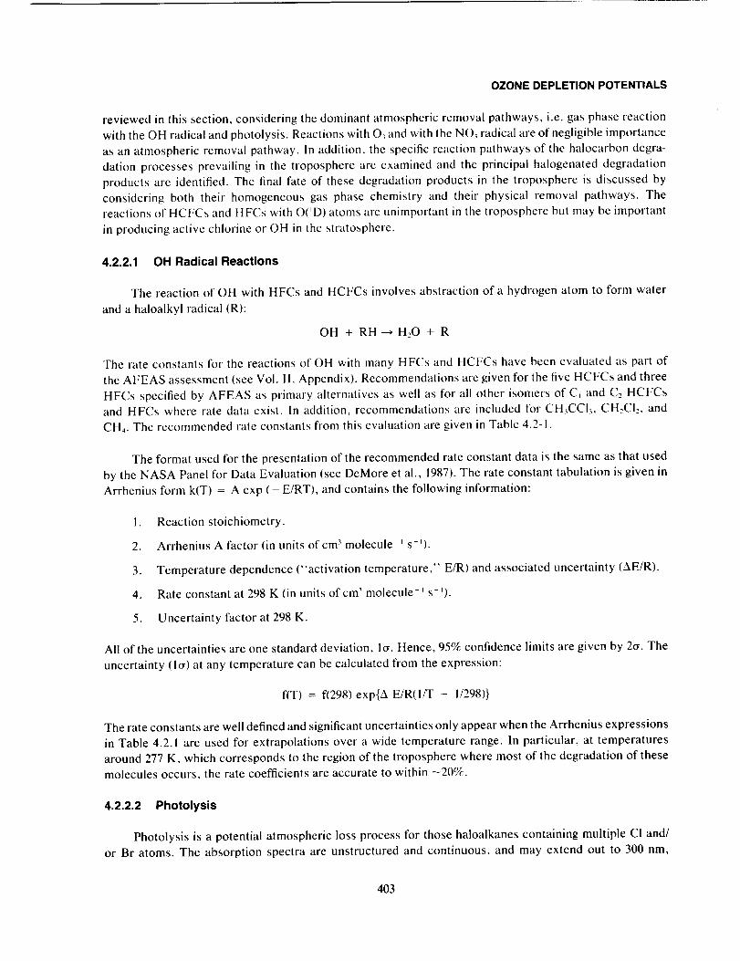
4.2.2.1 OH Radical Reactions
The reaction of OH with HFCs and HCFCs involves abstraction of a hydrogen atom to form water
and a haloalkyl radical (R):
OH + RH_ H20 + R
The rate constants for the reactions of OH with many HFCs and HCFCs have been evaluated as part of
the AFEAS assessment (see Vol. 11, Appendix). Recommendations are given for the five HCFCs and three
HFCs specified by AFEAS as primary alternatives as well as for all other isomers of C. and C2 HCFCs
and HFCs where rate data exist. In addition, recommendations are included for CH,CCI_, CH_CI_,, and
CH4. The recommended rate constants from this evaluation are given in Table 4.2-1.
The format used for the presentation of the recommended rate constant data is the same as that used
by the NASA Panel for Data Evaluation (see DeMore et al., 1987). The rate constant tabulation is given in
Arrhenius form k(T) = A exp ( - E/RT), and contains the following information:
I. Reaction stoichiometry.
2. Arrhenius A factor (in units ofcm 3 molecule ' s ').
3. Temperature dependence ("activation temperature," E/R) and associated uncertainty (AE/R).
4. Rate constant at 298 K (in units ofcm _ molecule _s-').
5. Uncertainty factor at 298 K.
All of the uncertainties are one standard deviation, 10.. Hence, 95% confidence limits are given by 20". The
uncertainty (I0") at any temperature can be calculated from the expression:
f(T) = f(298) exp{A E/R(I/T - 1/298)}
The rate constants are well defined and significant uncertainties only appear when the Arrhenius expressions
in Table 4.2.1 are used for extrapolations over a wide temperature range. In particular, at temperatures
around 277 K, which corresponds to the region of the troposphere where most of the degradation of these
molecules occurs, the rate coefficients are accurate to within -20%.
4.2.2.2 Photolysis
Photolysis is a potential atmospheric loss process for those haloalkanes containing multiple Cl and/
or Br atoms. The absorption spectra are unstructured and continuous, and may extend out to 300 nm,
403

OZONE DEPLETION POTENTIALS
Table 4.2-1. Recommended rate constants and uncertainties for reactions of OH withselected HFCs and HCFCs
Fluorocarbon
Reaction Number A ° E/R _ E/R b k_" f(298)
OH + CHFCI_, HCFC-2 I
OH + CHF2CI HCFC-22
OH + CHF3 HFC-23
OH + CH:CI_, 30
OH + CH.,FCI HCFC-31
OH + CHzF2 HFC-32OH + CHsF HFC-41
OH + Ell4 50
OH + CHCI2CF3 HCFC-123
OH + CHFCICF3 HCFC-124
OH + CHF:CFs HFC-125
OH + CH,CICF,CI HCFC- 132b
OH + CH2CICFs HCFC-133a
OH + CHF2CHF: HFC-134
OH + CH2FCFs HFC- 134aOH + CH3CCI3 140a
OH + CH3CFCI2 HCFC-141b
OH + CH3CFzCI HCFC-142b
OH + CH2FCHF2 HFC- 143
OH + CH3CF_ HFC- 143a
OH + CH2FCH2F HFC- 152
OH + CH3CHF., HFC-152aOH + CH3CH,F HFC-161
1.2d - 12)
i.2q - 12)
7.4_ - 13)
5.8_ - 12)
3.0q - 12)
2.5q - 12)
5.41 - 12)
2.3q - 12)
6.41 - 13)
6.6q - 13)
3.8q - 13)3.61 - 12)
5.21 - 13)
8.7(- 13)
1.7(- 12)
5.O(- 12)
2.7(- 13)
9.6( - 13)2.8(- 12)
2.6(- 13)
1.7(- l I)
1.5(- 12)
!.3(-I!)
1100_ 150 3.0(- 14) 1. I
1650___150 4.7(- 15) I.I
2350±400 2.1( - 16) 1.5
1100 ± 150 1.4( - 13) 1.2
1250± 150 4.5(- 14) 1.15
1650 +-200 1.0( - 14) 1.21700±300 1.8(- 14) 1.2
1700±200 7.7(- 15) 1.2
850_+ 150 3.7(- 14) 1.2
1250 ± 300 1.0( - 14) 1.2
1500+-500 2.5(- 15) 2.0
1600 ± 400 !.7( - 14) 2.0
1100 +-300 1.3( - 14) 1.3
1500 ± 500 5.7( - 15) 2.0
1750 ± 300 4.8( - 15) ! .21800±300 1.2(- 14) 1.3
1050± 200 7.5( - 15) 1.3
1650± 150 3.8(- 15) 1.2
1500 ± 500 1.8( - 14) 2.0
1500±500 !.7(- 15) 2.0
1500±500 I.I( - 13) 2.0
1100+-200 3.7( - 14) 1.1
1200±300 2.3(- 13) 2.0'_Units are cm 3 molecule _s '
bUnits are K
which could result in photodissociation in the troposphere. However, the cross sections are very low in
the long wavelength region, resulting in very low photolysis rates in the troposphere for fluorochloroalkanes
and brominated compounds such as CF_Br. Only for haloalkanes containing one Br and one or more CI
atoms (CF,CIBr, CHCI2Br, and CH,CIBr) or two or more Br atoms (CF2Br2, CH.,Brz, CHCIBr,, and CHBr,)
does photolysis in the troposphere become significant.
Solar photolysis is likely to contribute significantly to the stratospheric destruction of the alternative
fluorocarbons which have two or more chlorine atoms bonded to the same carbon atom.
The absorption cross sections for several HFCs and HCFCs have been reviewed as part of the AFEAS
assessment. Two of the eight HCFCs considered in the review, namely HCFC-123 and HCFC-141b, have
significant stratospheric photolysis. For these two species there is good agreement among the various
measurements of the ultraviolet cross sections in the wavelength region which is important for atmospheric
pholodissociation, that is, around 200 nm. There is also good agreement for HCFC-124, HCFC-22, and
HCFC-142b: these three species contain only one chlorine atom per molecule and OH reaction is the
dominant loss process in both the stratosphere and the troposphere.
404
OZONE DEPLETION POTENTIALS
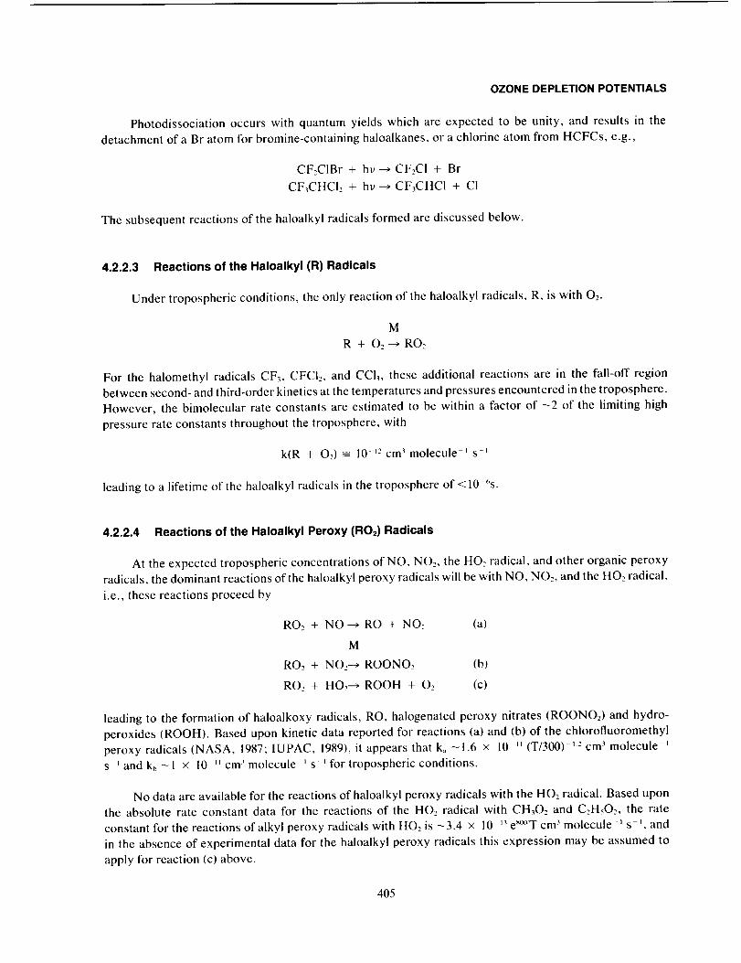
Photodissociation occurs with quantum yields which are expected to be unity, and results in the
detachment of a Br atom for bromine-containing haloalkanes, or a chlorine atom from HCFCs, e.g.,
CF2ClBr + hv--_ CF2CI + Br
CF_CHCI2 + hv--_ CF3CHC1 + Cl
The subsequent reactions of the haloalkyl radicals formed are discussed below.
4.2.2.3 Reactions of the Haloalkyl (R) Radicals
Under tropospheric conditions, the only reaction of the haloalkyl radicals, R, is with 02.
M
R + 02 _ RO2
For the halomethyl radicals CF3, CFCI2, and CC13, these additional reactions are in the fall-off region
between second- and third-order kinetics at the temperatures and pressures encountered in the troposphere.
However, the bimolecular rate constants are estimated to be within a factor of -2 of the limiting high
pressure rate constants throughout the troposphere, with
k(R + 09 _ 10 ,2cm _molecule ' s-'
leading to a lifetime of the haloalkyl radicals in the troposphere of < 10 %.
4.2.2.4 Reactions of the Haloalkyl Peroxy (RO2) Radicals
At the expected tropospheric concentrations of NO, NO:, the HO2 radical, and other organic peroxy
radicals, the dominant reactions of the haloalkyl peroxy radicals will be with NO, NO2, and the HO2 radical,
i.e., these reactions proceed by
RO2 + NO---* RO + NO: (a)
M
RO2 4- NO2---_ ROONO: (b)
RO2 + HO_,---* ROOH + 02 (c)
leading to the formation of haloalkoxy radicals, RO, halogenated peroxy nitrates (ROONO2) and hydro-
peroxides (ROOH). Based upon kinetic data reported for reactions (a) and (b) of the chlorofluoromethyl
peroxy radicals (NASA, 1987; IUPAC, 1989), it appears that k_, -1.6 × l0 _ (T/300) t2 cm 3 molecule-t
s _and kb --1 × 10 _ cm _ molecule ' s -_ for tropospheric conditions.
No data are available for the reactions of haloalkyl peroxy radicals with the HO2 radical. Based upon
the absolute rate constant data for the reactions of the HO2 radical with CH_O2 and C2H502, the rate
constant for the reactions of alkyl peroxy radicals with HO2 is -3.4 × 10 _ e"_"_'Tcm _molecule- _ s ', and
in the absence of experimental data for the haloalkyl peroxy radicals this expression may be assumed to
apply for reaction (c) above.
405
OZONE DEPLETION POTENTIALS
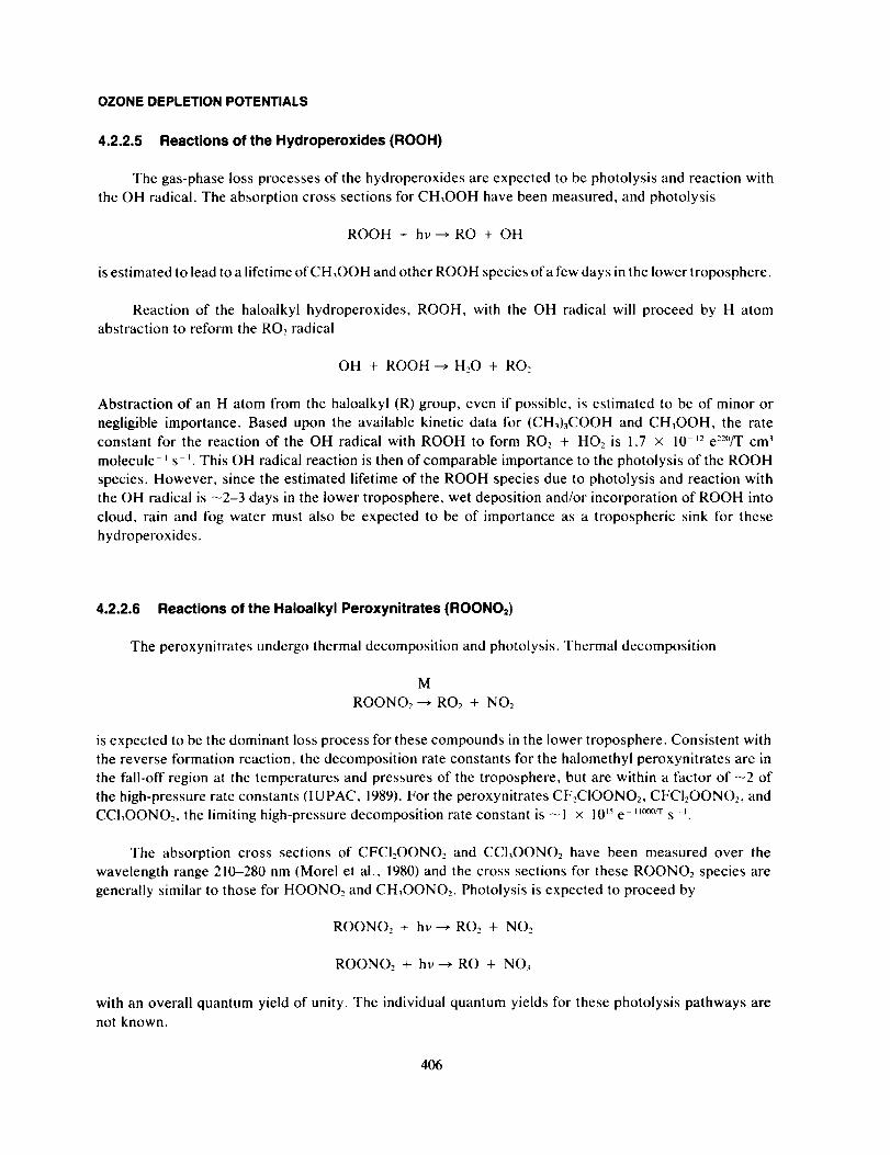
4.2.2.5 Reactions of the Hydroperoxides (ROOH)
The gas-phase loss processes of the hydroperoxides are expected to be photolysis and reaction with
the OH radical. The absorption cross sections for CH_OOH have been measured, and photolysis
ROOH + hv--_ RO + OH
is estimated to lead to a lifetime of CH3OOH and other ROOH species of a few days in the lower troposphere.
Reaction of the haloalkyi hydroperoxides, ROOH, with the OH radical will proceed by H atom
abstraction to reform the RO2 radical
OH + ROOH _ H20 + RO2
Abstraction of an H atom from the haloalkyl (R) group, even if possible, is estimated to be of minor or
negligible importance. Based upon the available kinetic data for (CH_)3COOH and CH3OOH, the rate
constant for the reaction of the OH radical with ROOH to form RO2 + HO2 is 1.7 x 10 -_2 e=°/T cm _
molecule-' s '. This OH radical reaction is then of comparable importance to the photolysis of the ROOH
species. However, since the estimated lifetime of the ROOH species due to photolysis and reaction with
the OH radical is -2-3 days in the lower troposphere, wet deposition and/or incorporation of ROOH into
cloud, rain and fog water must also be expected to be of importance as a tropospheric sink for these
hydroperoxides.
4.2.2.6 Reactions of the Haloalkyl Peroxynitrates (ROONO2)
The peroxynitrates undergo thermal decomposition and photolysis. Thermal decomposition
M
ROONO2---+ RO2 + NO2
is expected to be the dominant loss process for these compounds in the lower troposphere. Consistent with
the reverse formation reaction, the decomposition rate constants for the halomethyi peroxynitrates are in
the fall-off region at the temperatures and pressures of the troposphere, but are within a factor of -2 of
the high-pressure rate constants (IUPAC, 1989). For the peroxynitrates CF_C1OONO2, CFCI2OONO> and
CCI,OONO> the limiting high-pressure decomposition rate constant is -I x 10u e -_"X_':r s -_.
The absorption cross sections of CFCI2OONO2 and CCI3OONO2 have been measured over the
wavelength range 210-280 nm (Morel et al., 1980) and the cross sections for these ROONO2 species are
generally similar to those for HOONO2 and CH3OONO2. Photolysis is expected to proceed by
ROONO2 + hv---* RO: + NO__
ROONO2 + hv _ RO + NO_
with an overall quantum yield of unity. The individual quantum yields for these photolysis pathways are
not known.
406
OZONE DEPLETION POTENTIALS
The tropospheric reactions of the haloalkyl peroxy radicals lead ultimately to the corresponding
alkoxy radicals, RO.
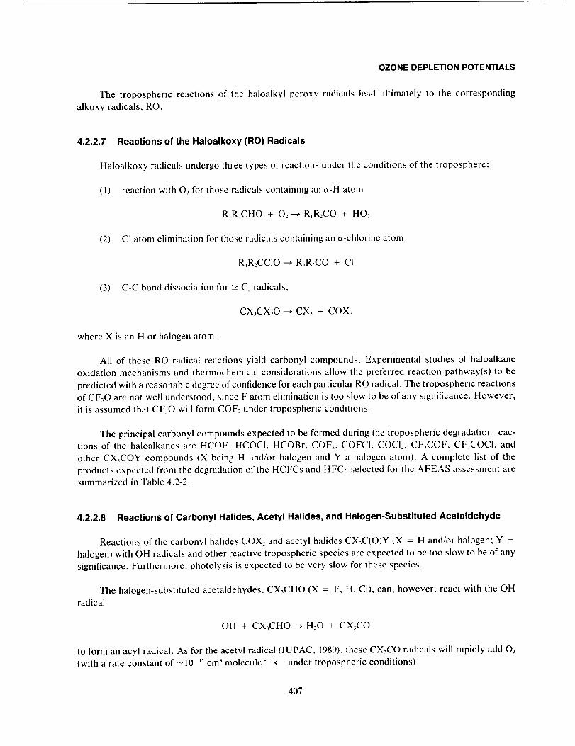
4.2.2.7 Reactions of the Haloalkoxy (RO) Radicals
Haloalkoxy radicals undergo three types of reactions under the conditions of the troposphere:
(I) reaction with O_ for those radicals containing an a-H atom
RIR2CHO + 02 _ RIR2CO + HO.,
(2) CI atom elimination for those radicals containing an a-chlorine atom
RIR_,CCIO---, RIR2CO + CI
(3) C-C bond dissociation for -> C2 radicals,
CX_CX_O--* CX_ + COX2
where X is an H or halogen atom.
All of these RO radical reactions yield carbonyl compounds. Experimental studies of haloalkane
oxidation mechanisms and thermochemical considerations allow the preferred reaction pathway(s) to be
predicted with a reasonable degree of confidence for each particular RO radical. The tropospheric reactions
of CF30 are not well understood, since F atom elimination is too slow to be of any significance. However,
it is assumed that CF30 will form COF2 under tropospheric conditions.
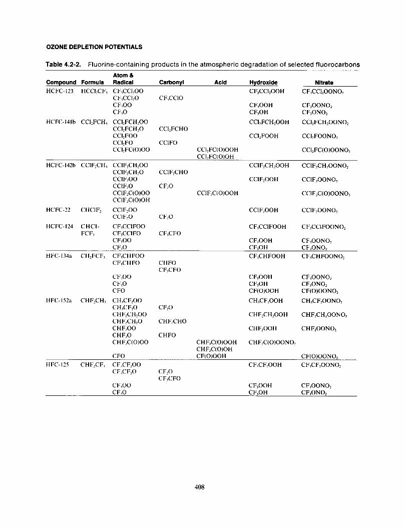
The principal carbonyl compounds expected to be formed during the tropospheric degradation reac-tions of the haloalkanes are HCOF, HCOCI, HCOBr, COF2, COFCI, COCI> CF,COF, CF,COCI, and
other CX,COY compounds (X being H and/or halogen and Y a halogen atom). A complete list of the
products expected from the degradation of the HCFCs and HFCs selected for the AFEAS assessment aresummarized in Table 4.2-2.
4.2.2.8 Reactions of Carbonyl Halides, Acetyl Halides, and Halogen-Substituted Acetaldehyde
Reactions of the carbonyl halides COX, and acetyl halides CX3C(O)Y (X = H and/or halogen; Y =
halogen) with OH radicals and other reactive tropospheric species are expected to be too slow to be of any
significance. Furthermore, photolysis is expected to be very slow for these species.
The halogen-substituted acetaldehydes, CX_CHO (X = F, H, CI), can, however, react with the OH
radical
OH + CX3CHO _ H20 + CX3CO
to form an acyl radical. As for the acetyl radical (IUPAC, 1989), these CX3CO radicals will rapidly add 02
(with a rate constant of-10-.2 cm , molecule _s _under tropospheric conditions)
407
OZONE DEPLETION POTENTIALS
Table 4.2-2. Fluorine-containing products in the atmospheric degradation of selected fluorocarbons
Atom &
Compound Formula Radical Carbonyl Acid Hydroxide Nitrate
HCFC-123 HCCI2CF3
HCFC-141b CCI2FCH_
CF3CCI2OO CF3CCI2OOH CFsCCI2OONOz
CF3CCI:O CF3CCIO
CF3OO CF3OOH CFsOONO2
CF30 CF3OH CF3ONO2
CCI2FCH2OO CCI2FCHzOOH CCI2FCH2OONO2
CCI.,FCH20 CCI2FCHO
CCI2FOO CCI2FOOH CCI2FOONO2
CCI2FO CCIFO
CCI2FC(O)OO CCI2FC(O)OOH CCI:FC(O)OONO2
CCI2FC(O)OH
HCFC-142b CC1F2CH3 CCIF2CH2OO CCIF2CH2OOH CCIF2CH2OONOz
CCIF2CHzO CCIFzCHO
CCIF2OO CCIF2OOH CCIF2OONO2
CCIF20 CF:O
CCIF2C(O)OO CCIF2C(O)OOH CCIF2C(O)OONO2
CCIF2C(O)OH
HCFC-22 CHCIF2 CCIF,OO CCIF2OOH CCIF2OONO2
CCIF20 CF20
HCFC-124 C HCI- CF3CCIFOO CF3CCIFOOH CF3CCIFOONO2
FCF, CF3CCIFO CF3CFO
CF3OO CF3OOH CF_OONO2
CF_O CF3OH CF3ONO2
HFC-134a CH2FCF3
HFC-152a CHF,CH_
CF_CHFOO CF3CHFOOH CF_CHFOONO2
CF_CHFO CHFOCF_CFO
CF_OO CF3OOH CF_OONO2
CF_O CFsOH CF3ONO2
CFO CF(O)OOH CF(O)OONO2
CH_CF2OO CH3CF2OOH CH3CFzOONO2
CH_CF.,O CF20
CHF,CH2OO CHF2CH2OOH CHFzCHzOONO2
CHF,CH20 CHF2CHO
CHF,OO CHF2OOH CHF2OONO2
CHF,O CHFO
CHF,C(O)OO CHF2C(O)OOH CHF2C(O)OONO2
CHF2C(O)OH
CFO CF(O)OOH CF(O)OONO2
HFC-125 CHF,CF_ CF_CF.,OO CF3CF2OOH CF3CF2OONO:
CF_CF20 CF20
CF,CFO
CF3OO CFsOOH CF3OONO2
CF30 CFsOH CF3ONO2
408
OZONE DEPLETION POTENTIALS
M
CX_CO + 02 _ CX_C(O)O:
to form acyl peroxy radicals. These radicals are expected to degrade ultimately to the carbonyl halides and
carbon dioxide. However, the CX_C(O)O: radicals are expected to form peroxynitrates by reaction with
NO_,:
CX,C(O)O: + NO:-_ CX_C(O)O2NO_
The peroxynitrate products are similar to the well-known peroxyacetyl nitrate (PAN) and are expected to
be thermally stable in the troposphere. In addition, photolysis of these halogenated peroxynitrates is
expected to be very slow and their residence time due to gas phase degradation could be long.
4.2.2.9 Physical Loss Processes
The low gas phase reactivity of many of the halogenated carbonyl compounds produced in the
degradation of HCFCs and HFCs leads to a potentially important role for physical loss process from the
atmosphere, i.e., incorporation into rain or clouds, or sea water, with subsequent hydrolysis. Although
handicapped by the total absence of Henry's law solubility data for any of the compounds of interest and
the limited availability of relevant kinetic data, an assessment of the rates and mechanisms of aqueous
phase removal of the gas phase degradation products has been carried out, as part of the AFEAS assessment.
The species X:CO, HXCO, CH3CXO, CF3OH, CX3OONO2, and ROOH (X = F or CI, R = halo-
substituted methyl or acetyl) are all expected to be removed from the atmosphere on time scales limited
by transport to cloudy regions or the marine boundary layer (i.e., about 1 month). Some support for this
comes from the recent measurements of COCI: by Wilson et al. (1988) in the troposphere and lower
stratosphere, which are consistent with a tropospheric physical loss process. Aqueous phase reactions of
these species result in the formation of chloride, fluoride, and carbon dioxide, as well as formic, acetic,
and oxalic acids. The species CX_CXO, CX_CX:OOH, CX_CXzOONO, CX,C(O)OONO2, and CXsC(O)OOH
are also expected to be removed from the atmosphere rapidly, and their aqueous phase reactions result in
the formation of halo-substituted acetates, CX,C(O)O.
The species CX3C(O)OH are very acidic and, as a result, are highly soluble in cloud water. These
acids are expected to be rapidly removed from the atmosphere by rainout. However, the aqueous phase
species CX3C(O)O are expected to be resistant to chemical degradation. Trichloroacetate can thermally
decompose on a time scale of2-l0 years to yield carbon dioxide and chloroform. In freshwater, the reaction
of CCI_C(O)O , CF3CIC(O)O may have very long aqueous phase lifetimes. The longest-lived species,
CF3C(O)O , could have a lifetime in natural waters as long as several hundred years. Processes which
could possibly degrade CF,CL ,,C/O)O on shorter time scales than suggested above, but whose rates
cannot be estimated with any degree of confidence at this time, include oxidation by photochemically
generated valence band holes in semiconductor particles and hydrolysis catalyzed by enzymes in micro-
organisms and plants: further research aimed at characterizing these processes is needed.
One possible gas phase degradation product about which very little is known is CF_ONO2. This
compound has never been observed, and may be thermally unstable. IfCF3ONO_ is thermally stable, then
it may have a long lifetime toward aqueous phase removal. Henry's law solubility data and hydrolysis
kinetics data for CF3ONO2 are needed before its aqueous phase removal rate can be assessed with any
degree of confidence.
409
OZONE DEPLETION POTENTIALS
4.2.2.10 Summary of Halocarbon Oxidation Chemistry
The following main conclusions concerning possible CFC substitutes can be drawn from the discussion
of halocarbon processes contained in this chapter and in the more detailed AFEAS assessment contained
in the Appendix to this report.
Tropospheric reaction with the OH radical is the major and rate determining loss process for the
HFCs and HCFCs in the atmosphere. The rate coefficients for the OH reactions are well defined at the
temperatures appropriate for tropospheric reaction. There are virtually no experimental data available
concerning the subsequent reactions occurring in the atmospheric degradation of these molecules. By
consideration of data for degradation of alkanes and chloroalkanes, it is possible to postulate the reaction
mechanism and products formed in the troposphere from HCFCs and HFCs. However, the results are
subject to large qualitative and quantitative uncertainty, and may even be incorrect.
A large variety of chlorine- and fluorine-containing intermediate products such as hydroperoxides,
peroxynitrates, carbonyl halides, aldehydes, and acids can be expected from the degradation of the
proposed CFC substitutes. Based on the available knowledge of gas phase chemistry, only four of these
products appear to be potentially significant carriers of chlorine to the stratosphere. These are CCIFO,
CF_CCIO, CCIF2CO_NO_, and CCI2FCO_NO2. However, physical removal processes may reduce this
potential. In addition, the possibility of pathways and products not predicted by the arguments-by-analogy
are a cause for concern.
A large part of the uncertainty of the mechanistic details of the HCFC oxidation arises from an
insufficient knowledge of the thermal stability and reactivity of halogenated alkoxy radicals. In particular,
the mechanism of oxidation of the CF_O radical, which is assumed to produce CF20, is not known for
atmospheric conditions and needs further study. Particular attention should also be paid to obtaining data
on the photochemistry, gas phase reactivity, and solubility of the carbonyl, acetyl, and formyl halides inorder to assess their removal rates and mechanisms.
Based on current knowledge, the products identified are unlikely to cause significant changes to the
effective greenhouse warming potential of the proposed CFC substitutes. This conclusion would be modified
if long-lived products such as CF_H were formed by unidentified pathways.
It would be prudent to carry out comprehensive laboratory tests and atmospheric measurements to
ascertain the validity of the proposed degradation mechanisms for HCFCs and HFCs, before large amountsof these substances are released to the environment.
4.2.3 Hydroxyl Radical Chemistry in the Troposphere
4.2.3.1 Processes Governing OH Concentration in the Troposphere
Following Weinstock's (1969) suggestion that reaction with OH radicals provides a major sink for
atmospheric CO and CH_, Levy (1971) was the first to propose that relatively high steady-state concentra-
tions of OH and other radicals might be present in the troposphere, as a result of photochemical reactions
involving ozone and other trace gases. Since that time, a comprehensive and relatively consistent theory
has been developed concerning the sources, chemical cycles, and sinks which control the OH concentration
in the troposphere.
410

OZONE DEPLETION POTENTIALS
The essential chemistry in the theory of tropospheric OH is illustrated in Figure 4.2-1. The steady-
state concentration of OH is determined by a balance between production and loss processes for free
radicals, and the fast interconversion reactions coupling OH with the hydroperoxy radical (HO2). The main
production route results from the photolysis of ozone at k < 320 nm to produce excited O('D) atoms. The
O(_D) atoms are mainly quenched to the ground state, but a significant fraction reacts with water vapor to
produce OH:
O3 + hv(_.< 320 nm)--, O('D) + O:
O(ID) + H20---, 2OH
It follows that the rate of OH production is proportional to the water vapor mixing ratio. In addition, the
photolysis of H202 organic hydroperoxides provide minor secondary sources of OH in the troposphere.
Because the hydroperoxyl radical, HOz, is rapidly converted to OH by reacting with NO and O_, photo-
chemical reactions leading to formation of HO2 provide a further, indirect source of OH. The most important
contribution of this type comes from the UV photolysis of formaldehyde, HCHO, which is present in the
troposphere as a result of the oxidation of CH4 and other volatile organic compounds:
HCHO + hv (_ < 330 nm)--_ H + HCO
HCO + O_---, HO2 + CO
H + O, + M---, HO: + M
Because CH4 oxidation is a chain reaction initiated by OH attack (see Figure 4.2-1), the organic oxidation
chemistry provides an amplification of the primary OH production resulting from ozone photolysis, as
emphasized by Warneck (1975).
Figure 4.2-1. Reactions governing concentrations of OH and H02
411
OZONE DEPLETION POTENTIALS
The loss processes involve combination reactions of the OH and HO2 radicals with each other and
also with NO, to form stable, non-radical products, e.g., H20, H202, HNO3, and HO2NO2. The more rapid
reactions of OH with CO and CH4 do not lead to overall loss of radicals since HO2 is formed, which is
cycled back to OH. Nevertheless, the steady-state concentration of OH is influenced by the concentrations
of reactive trace gases such as CH4, CO, Oa, and NO since these determine, through the fast interconversion
reactions, the partitioning of the total radical pool between OH and HO2.
The possible influence of cloud droplets and aerosol particles in providing heterogeneous loss mech-
anisms for HO_ free radicals has been considered by Warneck (1974). Aerosol loadings in the clean
troposphere are too low to provide significant sinks; but in the polluted boundary layer and in fogs and
clouds, heterogeneous loss of HO,, which has a longer chemical lifetime than OH, can be an important
factor in reducing the radical concentration. These factors combined with the dependence of OH on local
trace gas concentration lead to an expected large local variability in the concentrations of OH.
Since the dominant primary source of OH is the UV photolysis of ozone, a large seasonal, diurnal,
and latitudinal variation in the production rate is implied. Moreover, water vapor mixing ratio and cloudiness
will also influence OH production. These factors were discussed by Warneck (1975) and have subsequently
been investigated in detail in photochemical models of the troposphere, used to calculate globally averaged
tropospheric OH concentration (Crutzen and Fishman, 1977; Derwent and Curtis, 1977; Logan et al., 1981).
The models predict highest OH concentrations in the lower tropical troposphere with very low values in
polar regions.
At nighttime, there are no photochemical sources of OH. Nighttime free radical chemistry does occur,
however, as a result of initiation by attack of nitrate radicals on organic molecules, but OH steady-state
concentrations are much lower than in the sunlit atmosphere.
4.2.3.2 Validation of OH Photochemistry
In contrast to the well-developed theory of tropospheric OH, experimental measurements of OH
concentrations and verification of the theory have provided a challenge which has not yet been satisfactorilyovercome.
Three techniques for the time-resolved measurement of local OH concentrations have been developed
over a number of years, these being the '4C-tracer method, laser-induced fluorescence (LIF), and long-path
absorption spectroscopy (LPAS). Both the '4C-tracer method and the LIF technique are subject to a number
of potentially severe interferences, and the results of even the most recent measurements using these
techniques must be treated with caution. To date the UV LPAS technique appears to give the most reliable
measurements. The most recently developed high resolution instrument (Dorn et al., 1988; Platt et al.,
1988) overcomes interference problems by detecting a spectral range covering several OH absorption
features. This method gives absolute OH concentrations and does not require calibration. The only
information needed for data analysis is the oscillator strength for OH which is known to be better than 5%.
The daytime OH measurements published over the last four years using all three techniques vary
between approximately 0.4 and 9 x 10" OH radicals per cm _, which is broadly consistent with current
model predictions. Validation of a time-dependent model, however, requires not only the measurement of
OH itself, but also the simultaneous determination of all input parameters that control the local OH
chemistry. In the recent LPAS measurements, sufficient supporting data were obtained to allow full model
412
OZONE DEPLETION POTENTIALS
calculation of the expected local OH concentrations (Perner et al., 1987). Comparison of these recent
experimental results with the model calculations leads to the following conclusions:
I. In the presence of high NO_ concentrations (>2 ppbv), the steady-state OH concentration is
controlled only by the primary source term (ozone photolysis and subsequent reaction of O('D)
atoms with water vapor) and one main loss reaction (OH + NOz forming nitric acid). Thus the
calculation of OH concentrations needs only measurements of O_, J(O'D), H__O, and NO_, with
the most critical being the correct determination of J(O'D). In this case the measurements agree
with the calculated OH concentrations to within -50%.
2. In relatively clean air (NO_< 1 ppbv), the OH concentration calculated using a detailed model
with the supporting measurements as input parameters exceeded the measured concentrations
by about a factor of two. This implies an inadequate description of the HO_ losses in the model.
Further development of techniques for OH measurements are clearly necessary and confidence in
the measurements would be aided by a successful intercomparison of more than one system. Also, there
is a need for measurements at different characteristic locations, in particular at high altitudes remote from
local terrestrial sources of gases and particles.
4.2.3.3 Indirect Determination of Global Hydroxyl Radical
Indirect methods for determining the OH abundance from trace gas budget considerations have
provided the best test for global models of OH distribution. In principle, any molecule can be used provided
that the following conditions are satisfied.
• Its removal occurs by reaction with OH alone and the rate of this removal is accurately known
both as a function of temperature and pressure.
• Its atmospheric abundance is accurately known.
• The source strength and distribution in time and space is accurately known.
While many chemicals (e.g., CO, non-methane hydrocarbons [NMHC]) are nearly exclusively removed
by OH radicals, it has not been possible to use them because their sources are diverse and often unknown.
However, in two cases the above conditions are met to varying degrees: man-made halocarbons and
naturally occurring '4CO. In recent decades synthetic ha[ogenated chemicals have been injected into the
environment in such significant amounts that a measurable global background is present. Because of the
exclusive man-made source of halocarbons, the major uncertainties associated with the source term can,
in principle, be eliminated. A select group of these halocarbons are also removed from the atmosphere
nearly exclusively by reaction with OH. Similarly, '4CO has a well-defined cosmic ray source and its
atmospheric abundance can be related to OH. In the following paragraphs previous attempts to evaluate
OH abundance in this way are summarized and a recent assessment of the global OH concentrations and
resultant halocarbon lifetimes conducted within AFEAS is presented.
Methyl chloroform and the hydroxyl radical
A first demonstration of this technique was presented by Singh (1977a, b) and Lovelock (1977), who
selected methyl chloroform (CH3CCI0 as the currently most suitable OH-tracer fulfilling the above criteria.
413
OZONE DEPLETION POTENTIALS
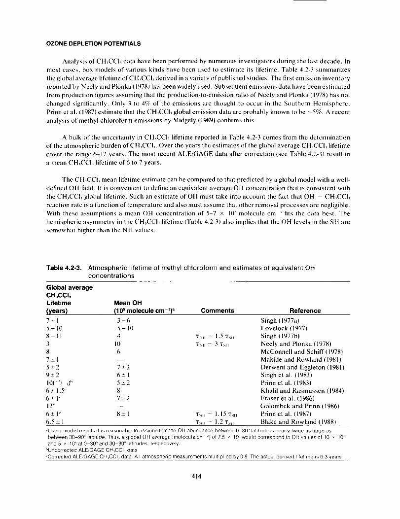
Analysis of CH,CCL data have been performed by numerous investigators during the last decade. In
most cases, box models of various kinds have been used to estimate its lifetime. Table 4.2-3 summarizes
the global average lifetime of CH,CCI, derived in a variety of published studies. The first emission inventory
reported by Neely and Plonka (1978) has been widely used. Subsequent emissions data have been estimated
from production figures assuming that the production-to-emission ratio of Neely and Plonka (1978) has not
changed significantly. Only 3 to 4% of the emissions are thought to occur in the Southern Hemisphere.
Prinn et al. (1987) estimate that the CH,CCL global emission data are probably known to be --5%. A recent
analysis of methyl chloroform emissions by Midgely (1989) confirms this.
A bulk of the uncertainty in CH_CC1, lifetime reported in Table 4.2-3 comes from the determination
of the atmospheric burden of CH,CCI,. Over the years the estimates of the global average CH,CCI, lifetime
cover the range 6-12 years. The most recent ALE/GAGE data after correction (see Table 4.2-3) result in
a mean CH,CCL lifetime of 6 to 7 years.
The CH,CCL mean lifetime estimate can be compared to that predicted by a global model with a well-
defined OH field. It is convenient to define an equivalent average OH concentration that is consistent with
the CH3CCI, global lifetime. Such an estimate of OH must take into account the fact that OH + CH_CCI3
reaction rate is a function of temperature and also must assume that other removal processes are negligible.
With these assumptions a mean OH concentration of 5-7 × 10 ' molecule cm ' fits the data best. The
hemispheric asymmetry in the CH3CCI, lifetime (Table 4.2-3) also implies that the OH levels in the SH are
somewhat higher than the NH values.
Table 4.2-3. Atmospheric lifetime of methyl chloroform and estimates of equivalent OHconcentrations
Global average
CH3CCI3Lifetime Mean OH
(years) (10 s molecule cm-_)" Comments Reference
7_+1 3-65- I0 5- 10
8 I1 4
3 10
8 6
7+_1
5_+2 7_+2
9+2 6_+1
10( "'/ d" 5 _+26_+ 1.5 _ 8
6+1 _ 7-+2
12b
6+1 _ 8_+1
6.5_+1TNH _ 1.15 "rs.
TN. _ 1.2"rs.
Singh (1977a)Lovelock (1977)
Singh (1977b)
Neely and Plonka (1978)
McConnell and Schiff (1978)
Makide and Rowland (1981)
Derwent and Eggleton (1981)
Singh et al. (1983)Prinn et al. (1983)
Khalil and Rasmussen (1984)
Fraser et al. (1986)
Golombek and Prinn (1986)Prinn et al. (1987)
Blake and Rowland (1988)
"Using model results it is reasonable to assume that the OH abundance between 0-30 ° latitude is nearly twice as large as
between 30-90 ° latitude. Thus, aglobaIOHaverage(moleculecm :_)of 75 x 10 _' would correspond to OH values of 10 x 10 s
and 5 x 10 _' at 0-30 ° and 30 90 ° latitudes, respeclively.
_'Uncorrected ALE/GAGE CH3CCI:_ data.
'Corrected ALE/GAGE CH:_CCI_ data All atmospheric measurements multiplied by 08 The actual derived lifetime is 6.3 years.
414
OZONE DEPLETION POTENTIALS
Other halocarbons have been used in a similar manner to estimate OH, for example, dichloromethane,
1,2 dichloroethane and tetrachloroethene (Singh et al., 1983). A two-box model shows that removal rates
of these molecules are consistent with average OH concentrations of 4 to 5 x 10' molecules cm _. Because
of their relatively short lifetimes (several months) compared to CH3CCI_, these chemicals could potentially
reveal OH latitudinal and seasonal gradients with greater sensitivity. However, their source strengths are
not as well defined as that of CH3CCI_. In addition, these analyses are sensitive to the seasonal variations
in emissions which are poorly known.
14CO and the hydroxyl radical
The first attempts to calculate the global mean tropospheric hydroxyl concentration from isotopic
distribution in atmospheric carbon monoxide were made by Weinstock (1969) and by Weinstock and Niki
(1972). They used the three available _4CO measurements by McKay et al. (1963), an estimate of the global
source strength for '4CO from the well-known cosmic ray bombardment of atmospheric nitrogen molecules,
and the OH + CO rate coefficient to derive an estimate for the atmospheric turnover time for _-'CO of the
order of 1 month. Furthermore, they suggested that OH radicals were responsible for the CO removal and
obtained an estimate of the global mean OH abundance.
The '4CO concentrations in the troposphere are extremely small with a winter maximum of 20 molecule
cm 3 and a summer minimum of about 10 molecule cm _. Volz et al. (1981) improved the methodology
based on four refinements, viz:
• additional measurements of '4CO in the lower troposphere,
• evaluated chemical kinetic data for the OH + CO reaction, and
• a global two-dimensional time-dependent model to investigate the coupled CH4-H,-CO-NO,-O3
life cycles, replacing the box model approach.
These analyses led Volz et al. (1981) to obtain a mean tropospheric OH concentration of 6.5 ÷3_2 x I0'
molecule cm -3. No additional data on '4CO have been collected in the intervening years and no Southern
Hemispheric data are available. Derwent and Volz-Thomas (1989) in a re-evaluation of this technique
conclude that the average OH derived by this method remains unchanged.
4.2.3.4 Recent Assessment of Tropospheric OH Abundance and Halocarbon Lifetimes
The above summary shows that an overall volume-averaged OH concentration of 6 {m2) x 10-_
molecule cm ' best represents all of the available information on the CH_CCI, and '4CO budgets. However,
the usefulness of a global mean OH concentration for determination of overall reaction rates and lifetimes
of HCFCs derived in this fashion is questionable. This arises because of the non-uniformity of the OH
abundance and of the distribution of the molecules with which it reacts, and also because of the different
temperature dependencies of the reaction rates in the troposphere. In the recent AFEAS assessment these
factors were considered at some depth. Prather (1989) used 3-dimensional tropospheric OH fields that were
calculated from a climatology of sunlight, temperature, and trace gas mixing ratios. These OH fields were
then used to study the methyl chloroform budget by calculating the integrated loss of this molecule in a 3-
D chemical transport model of the troposphere and to test the accuracy of scaling the HCFC lifetimes to
an assumed methyl chloroform lifetime.
415
OZONE DEPLETION POTENTIALS
In the AFEAS assessment, the lifetimes of HCFCs and HFCs were determined by three separate
approaches:
I. 2-D chemical transport model with semi-empirical fit to '4CO:
2. Photochemical calculation of 3-D OH fields and integrated loss;
3. Scaling of the interred CH_CCI, lifetime by rate coefficients.
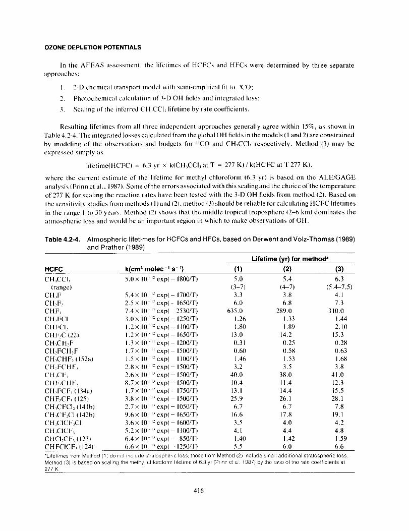
Resulting lifetimes from all three independent approaches generally agree within 15%, as shown in
Table 4.2-4. The integrated losses calculated from the global OH fields in the models ( 1 and 2) are constrained
by modeling of the observations and budgets for '4CO and CH,CCI, respectively. Method (3) may be
expressed simply as
lit'etime(HCFC) = 6.3 yr × k(CH_CCI_ at T = 277 K) / k(HCFC at T 277 K),
where lhe current estimate of the lifetime for methyl chloroform (6.3 yr) is based on the ALE/GAGE
analysis ( Prinn et al., 1987). Some of the errors associated with this scaling and the choice of the temperature
of 277 K for scaling the reaction rates have been tested with the 3-D OH fields from method (2). Based on
the sensitivity studies from methods (1) and (2), method (3) should be reliable for calculating HCFC lifetimes
in the range I to 311years. Method (2) shows that the middle tropical troposphere {2-6 km) dominates the
atmospheric loss and would be an important region in which to make observations of OH.
Table 4.2-4. Atmospheric lifetimes for HCFCs and HFCs, based on Derwent and Volz-Thomas (1989)
and Prather (1989)
Lifetime (yr) for method"
HCFC k(cm 3 molec -' s -') (1) (2) (3)
CH_CCI_ 5.0× 10 ,2 exp(- 1800/T) 5.0 5.4 6.3
(range) (3-7) (4-7) (5.4-7.5)
CHeF 5.4× 10 ': exp(- 1700/T) 3.3 3.8 4.1
CH,F2 2.5 × 10 '-_exp( - 1650/T) 6.0 6.8 7.3CHF_ 7.4 × 10 '_ exp( - 2530/T) 635.0 289.0 310.0
CH,FCI 3.0× l0 '-"exp(- 1250/T) 1.26 1.33 1.44
CHFCI, 1.2 × 10 '-"exp(- 1100/T) 1.80 1.89 2.10
CHFzC (22) 1.2× 10 ,2 exp( 1650/T) 13.0 14.2 15.3
CH_CHzF 1.3 × 10 " exp(- 1200/T) 0.31 0.25 0.28
CHzFCH:F 1.7 × 10 " exp(- 1500/T) 0.60 0.58 0.63
CH_CHF:(152a) 1.5×10 'eexp( 1100/T) 1.46 1.53 1.68
CH:FCHF, 2.8 × l0 '-"exp( - 1500/T) 3.2 3.5 3.8
CH,CF, 2.6×10 '_exp( 1500/T) 40.0 38.0 41.0CHF:CHF, 8.7 × 10 '_ exp( - 1500/T) 10.4 ! 1.4 12.3
CH:FCF, (134a) 1.7 × 10 '-"exp( - 1750/T) 13. I 14.4 15.5
CHF,CF, (125) 3.8 × l0 '_ exp( - 1500/T) 25.9 26.1 28.1
CH,CFCI, (141b) 2.7 × 10 '' exp(- 1050/T) 6.7 6.7 7.8
CH_CF:CI (142b) 9.6× 10 '_ exp( - 1650/T) 16.6 17.8 19.1
CH:CICFzCI 3.6 × 10 ,e exp( - 1600/T) 3.5 4.0 4.2
CH, CICF_ 5.2 × 10 '_ exp( - 1100/T) 4. I 4.4 4.8
CHCleCF_ (123) 6.4 × 10 '; exp(- 850/T) 1.40 1.42 1.59
CHFCICF_ (124) 6.6 × 10 '_ exp( - 1250/T) 5.5 6.0 6.6
*Lifetimes from Method (1) do not include stratospheric loss; those from Method (2)include small additional stratospheric loss.Method (3) is based on scaling the melhyl chloroform liletime of 63 yr (Prinn el al. 1987) by the ratio of the rate coefficients at277 K
416
OZONE DEPLETION POTENTIALS
Estimated uncertainties in the HCFC and HFC lifetimes between I and 30 years are + 50% for (1)
and _+ 40% for (3) and (2). These ranges include the uncertainty in the rate constants for the OH reactions.
Global OH values that give lifetimes outside of these ranges of uncertainty are inconsistent with detailed
analyses of the observed distributions for _4CO and CH_CCI_. The expected spatial and seasonal variations
in the global distribution of HCFCs with lifetimes of 1 to 30 years have been examined with methods (1)
and (2) and found to have insignificant effect on the calculated lifetimes. Larger uncertainties apply to gases
with lifetimes shorter than one year: however, for these species our concern is for destruction on a regional
scale rather than global accumulation.
Clearly any changes in the concentrations of ozone and other trace gases in the troposphere, which
affect OH abundance, will have an impact on HCFC lifetimes and in the following section we review the
relevant tropospheric chemistry and current perception of future atmospheric behavior in this context.
4.2.4 Tropospheric Chemistry Influencing OH and Ozone
4.2.4.1 Processes Controlling Tropospheric Ozone
Tropospheric ozone may be produced by in situ chemistry (Crutzen, 1973; Chameides and Walker,
1973; Fishman and Crutzen, 1978) or by transfer from the stratosphere, where 03 is generated by the
photodissociation of molecular oxygen at altitudes above 25 km, followed by combination of the ground
state oxygen atoms with 02:
O: + hv (h< 245 nm) ---, 2OOP)
O('P) + O: + M---, O, + M
The in situ source of tropospheric ozone is the reaction of HO-, or organic peroxy radicals with NO
followed by the photodissociation of the nitrogen dioxide produced and the O(3P) + O-, reaction.
HO: + NO_ NO, + OH
NO-, + hv (h < 400 nm)---, O(_P) + NO
Although NO and NOz concentrations are very low throughout most of the troposphere, the effect of
this reaction sequence can provide a significant O_ source.
Ozone is also consumed in the troposphere as a result of photodissociation in the ultraviolet region.
Most of the excited O(_D) atoms are quenched by N_, and 02 to the ground state, O('P), which reform
ozone, but that fraction which reacts with other trace molecules (e.g., with water to produce OH), represents
a net loss of ozone. Photolysis of ozone in the near UV (Huggins bands) and visible (Chappuis bands) does
not lead to net ozone loss. There is also an in situ loss of ozone through reaction with NO, (to give NO0,
HO2 and unsaturated hydrocarbons. Model calculations (e.g., Levy et al., 1985) point to an approximate
balance between in situ sources and sinks for tropospheric ozone, averaged over the globe. This is consistent
with estimates of the magnitude of the surface sink for ozone, which averaged over the globe, is approxi-
mately equal to the stratospheric injection. However, analysis of observations and regional budgets (Logan,
1985; Bojkov, 1986; Penkett, 1988) show a clear indication that Northern Hemisphere tropospheric ozone
is increasing. Changes in the seasonal modulation of ozone concentration, and in the man-made emissions
and concentration of trace gases which affect ozone, suggest that the increase is due to a shift in the balance
between in situ production and loss (Penkett, 1988). This balance essentially depends on the amount of
417
OZONE DEPLETION POTENTIALS
NO_ present in the background atmosphere together with the concentration of peroxy radicals derived
from oxidation of CO, CH4 and non-methane hydrocarbons, which controls the flux through the reactions
in which NO is oxidized to NO.,.
RO: + NO _ NO. + RO (R = H or organic radical)
The amount of tropospheric ozone is clearly central to the problem of the oxidizing efficiency of the
troposphere, since O_ photolysis is the primary source of OH radicals as well as being an oxidizing species
itself. It follows that the future trends of oxidizing capacity will be tied to the future tropospheric burden
of CO, CH4, non-methane hydrocarbons and other organics, as well as nitrogen oxides. We now summarize
the current picture of the distribution of ozone precursors in the troposphere. The distribution of ozone
itself in the troposphere is covered in the assessment of global ozone concentrations in Chapter 2.
4.2.4.2 Tropospheric Distribution of Reactive Nitrogen Species
The tropospheric lifetime of NO_ (NO + NO.,) is rather short and consequently it is not possible to
define an average, representative NO_ mixing ratio on a hemispheric or global scale.
The NO, levels in urban and industrial areas are determined largely by anthropogenic sources. This
leads to near surface NOx mixing ratios in rural areas of the eastern United States and Western Europe
typically in the range between 1 ppbv and I0 ppbv. In less populated and coastal regions, the NO_ levels
depend on the prevailing meteorology and the proximity and distribution of urban sources. In these locations
the NO_ mixing ratios typically range between 0. I and 1 ppbv.
Surface measurements at remote locations reflect the influence of natural sources, such as soil
emissions and lightning, which are principally terrestrial sources that are seasonal. These sources may
provide surface concentrations of NO_ that typically range between 0.02 ppbv and 0. I ppbv (Fehsenfeld et
al., 1988). It should be noled that at most locations on land, particularly in the mid-latitudes, the NO_ levels
in ambient air are influenced by anthropogenic activities. In remote maritime air and in the polar regions
that are not influenced by anthropogenic activities, the NO_ concentrations are exceedingly small, typically
0.001 ppbv to 0.01 ppbv, and are associated with the downward mixing of NO_ from NO_ reservoirs in the
upper troposphere.
The free tropospheric burden of NO_ is also strongly influenced by anthropogenic NO_, particularly
from combustion sources in the Northern Hemisphere. Variability in the atmospheric transport and pho-
tochemical lifetimes, together with the contribution of aircraft emissions of NOx and natural sources such
as lightning and stratospheric subsidence, increases the variability of N(L concentration in the free tro-
posphere. Here the NO, mixing ratios may vary from 0.02 ppbv in remote regions to 5 ppbv over populated
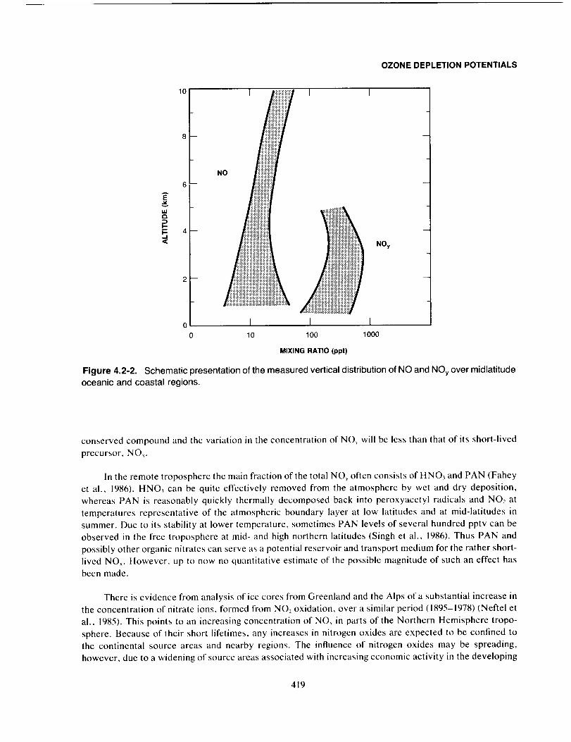
areas. In general, throughout the free troposphere the NOn mixing ratio increases with height, as illustrated
by the NO distribution shown in Figure 4.2-2.
The distribution of NOy (NO_: sum of all oxidized nitrogen species except N20 = NO + NO,,+
NO,+ 2 x N20_+ HNO,+ PAN + HO2NO_,+ organic nitrates) is very similar to that of the source
compound NO_. Near the sources the majority of NOy is in the form of NO,. However, the NO_ will be
rapidly converted to PAN, HNO3, or other NOy compounds. For example, during periods of maximum
insolation the photochemical lifetime of NO_ is less than one day. Thus, in the remote free troposphere
NO_ accounts for only a small fraction (approximately 10%) of the NOy . For this reason, NOy is a more
418
OZONE DEPLETION POTENTIALS
14.1a
i-I-,-I
lO 1 I I
NO
NOy
I I I10 100 1000
MIXING RATIO(ppt)
Figure 4.2-2. Schematic presentation of the measured vertical distribution of NO and NOy over midlatitude
oceanic and coastal regions.
conserved compound and the variation in the concentration of NO_ will be less than that of its short-lived
precursor, NO_.
In the remote troposphere the main fraction of the total NOy often consists of HNO_ and PAN (Fahey
et al., 1986). HNO3 can be quite effectively removed from the atmosphere by wet and dry deposition,
whereas PAN is reasonably quickly thermally decomposed back into peroxyacetyl radicals and NO, at
temperatures representative of the atmospheric boundary layer at low latitudes and at mid-latitudes in
summer. Due to its stability at lower temperature, sometimes PAN levels of several hundred pptv can be
observed in the free troposphere at mid- and high northern latitudes (Singh et al., 1986). Thus PAN and
possibly other organic nitrates can serve as a potential reservoir and transport medium for the rather short-
lived NOx. However, up to now no quantitative estimate of the possible magnitude of such an effect has
been made.
There is evidence from analysis of ice cores from Greenland and the Alps of a substantial increase in
the concentration of nitrate ions, formed from NO2 oxidation, over a similar period (1895-1978) (Neftel et
al., 1985). This points to an increasing concentration of NO_ in parts of the Northern Hemisphere tropo-
sphere. Because of their short lifetimes, any increases in nitrogen oxides are expected to be confined to
the continental source areas and nearby regions. The influence of nitrogen oxides may be spreading,
however, due to a widening of source areas associated with increasing economic activity in the developing
419
OZONE DEPLETION POTENTIALS
world and due to reservoir species such as peroxyacetyl nitrate (PAN), which are formed in NMHC-NO,
interactions and which have relatively long atmospheric lifetimes and can dissociate to produce NOz far
from source regions.
4.2.4.3 Tropospheric Distribution of Hydrocarbons and CO
The most important and abundant atmospheric hydrocarbon is methane. Its global distribution is well
established and it exhibits only a relatively small variability in the background troposphere. The Northern
Hemispheric CH4 mixing ratios are about 1.7 ppm, the Southern Hemispheric levels are slightly lower,
about 1.6 ppm.
CO has a considerably lower tropospheric abundance, but due to its higher reactivity towards OH
radicals it is very important for the oxidizing efficiency of the atmosphere. The tropospheric distribution
of CO is reasonably well known and there is a significant interhemispheric gradient. CO mixing ratios in
the Southern Hemisphere are around 50-70 ppbv, and roughly a factor 2-3 higher in the Northern Hemi-
sphere. A distinct seasonal variation in CO levels in both hemispheres has been identified. However, global
coverage of CO distribution is still inadequate.
The current picture of the distribution of non-methane hydrocarbons (NMHC) in the troposphere is
still far from complete due in part to the limited number of investigations, and there is large variability in
the background concentrations. This variability results from the relatively short average atmospheric
residence times, which range from a few hours to a few months. Also, the different NMHCs have various
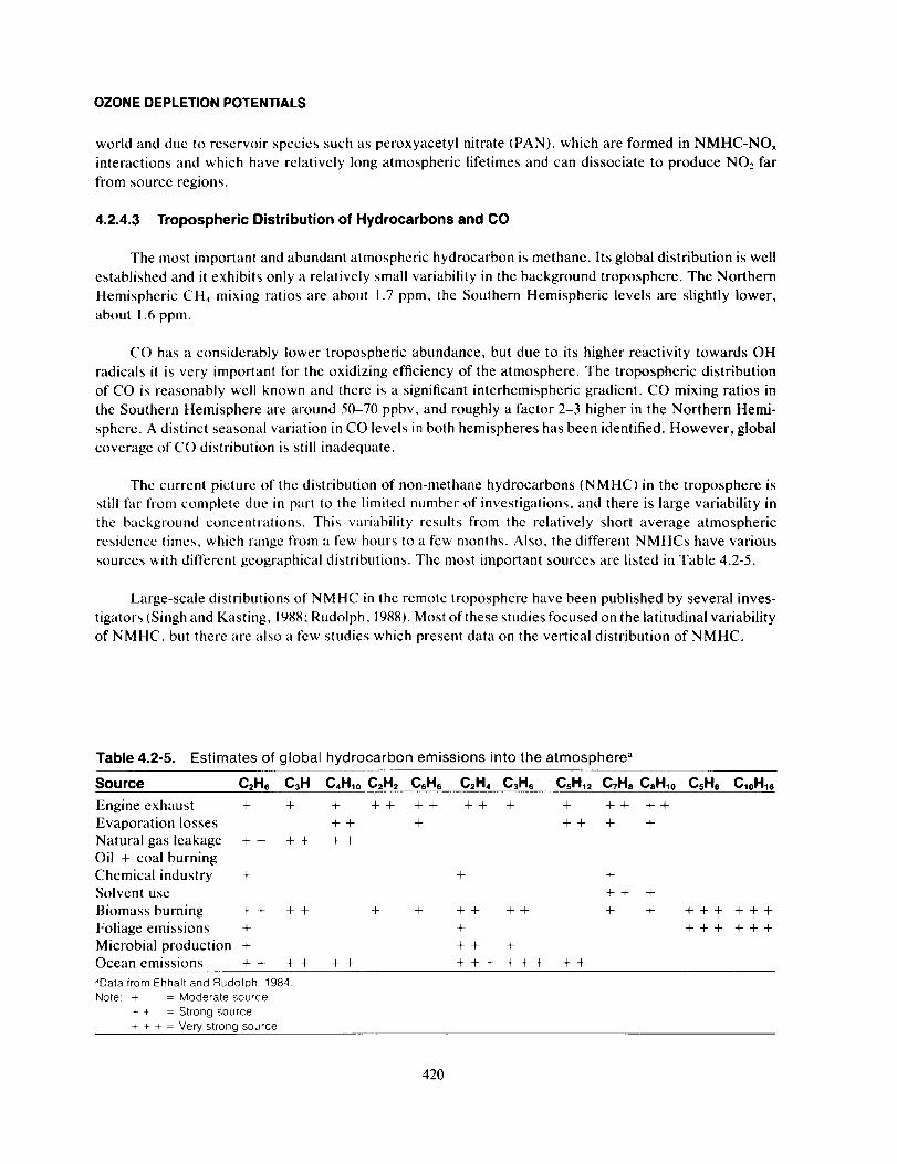
sources with different geographical distributions. The most important sources are listed in Table 4.2-5.
Large-scale distributions of NMHC in the remote troposphere have been published by several inves-
tigators (Singh and Kasting, 1988; Rudolph, 1988). Most of these studies focused on the latitudinal variability
of NMHC, but there are also a few studies which present data on the vertical distribution of NMHC.
Table 4.2-5. Estimates of global hydrocarbon emissions into the atmosphere a
Source C2He C3H C4H10 C2H2 C6He C2H4 C3He CsH12 CTHe C8Hlo CsH8 CloHle
Engine exhaust + + + + + ++ + + + + ++ ++
Evaporation losses + + + + + + +Natural gas leakage + + + + + +
Oil + coal burning
Chemical industry + + +Solvent use + + +
Biomass burning + + + + + + + + + + + +
Foliage emissions + +
Microbial production + + + +Ocean emissions ++ ++ ++ +++ +++ ++
+++ ++++++ +++
"Data from Ehhalt and Rudolph, 1984.
Nole: + - Moderate source
_, + - Strong source
+ + + Very strong source
420

OZONE DEPLETION POTENTIALS
The distribution of the longer-lived NMHC ('r > 1 week) show some systematic features which can
be ascribed to a representative latitudinal profile. On the average the highest mixing ratios are observed at
mid- to high northern latitudes, roughly 1-3 ppbv of ethane, 0.2-0.6 ppbv of propane and n-butane, 0.1-
0.5 ppbv of acetylene, 0.05-0.25 ppbv of benzene, and 0.02-0. ! ppbv of i-butane. In general, all these
species show a considerable decrease towards lower latitudes and this gradient is more pronounced for the
shorter-lived of these NMHC. This reflects both the source distribution with high emissions in the indus-
trialized zone of the Northern Hemisphere and the faster removal at low latitudes due to the higher OH
radical concentrations at tropical latitudes. Average Southern Hemisphere mixing ratios are roughly 0.15-
0.4 ppbv ethane, 0.03-0.1 ppbv propane, 0.01-0.05 ppbv n-butane, 0.01-0.05 ppbv acetylene, 0.01-0.03
ppbv benzene, and 0.005-0.03 ppbv i-butane. There is a clear seasonal cycle in the troposphere mixing
ratios of the light aliphatic hydrocarbons, with substantially higher values in the winter months. The cycle
is consistent with predominant removal of these hydrocarbons by reaction with OH.
There seems to be a slight but systematic decrease from low southern latitudes towards mid southern
latitudes. For ethane and probably the other hydrocarbons, there seems to be a significant and systematic
seasonal cycle. In both hemispheres the minima are in the respective late summer, maxima in late winter.
For more reactive NMHC with average atmospheric residence times of less than one week, it is no
longer justified to consider their distributions as being systematic with latitude. These atmospheric con-
centrations are determined by emissions, removal reactions, and transport on a local or regional scale (up
to several hundred km). The most important NMHC in this category (I week > "r > 0.5 days) are C2-C5
alkenes and, to a lesser extent, < C5 alkanes and alkylbenzenes. Since the sources of C_,-C_ alkenes include
biomass burning, emissions from vegetation, and emissions from oceans, substantial concentrations in the
range from 0.1 to a few ppbv ofethene and propane have been observed over nonindustrialized continental
regions and the oceans.
The extremely reactive terpenes and isoprene in general show a very strong decrease with increasing
altitude and can generally only be observed near their sources within the atmospheric boundary layer.
Over areas with dense vegetation, isoprene mixing ratios around 0.5-2 ppbv and monoterpene mixing
ratios approaching I ppbv are frequently observed (Rasmussen and Khalil, 1988; Zimmerman et al., 1988).
The emissions of many biogenic NMHC strongly depend on temperature, relative humidity, and light
intensity. The types of emitted compounds also depend on the type of vegetation, e.g., isoprene is primarily
emitted from deciduous plants whereas coniferous trees mainly act as terpene sources. The estimated
global emission rate of isoprene is about 480 x 1012 g yr ' (Rasmussen and Khalil. 1988). Comparable
emission rates have been estimated for the other terpenoid compounds.
The global source strength of all NMHCs, but not including isoprene and the terpenes, is estimated
to be about 100-130 × 10 _2g yr _.Since these NMHC emission estimates are highly uncertain and probably
underestimated, we cannot yet make any quantitative estimates on the contribution of NMHC to the
tropospheric O_ and OH concentrations. Also, the atmospheric oxidation of NMHC leads to the in situ
production of CO, which has a longer residence time than the NMHC and could extend their influence
over a wider spatial regime. A comparison with the global CH4 emission rate of about 400 x 10 t-_g yr-'
shows that the possible contribution of NMHC (not including isoprene and terpenes) can be quite substan-
tial. The influence of isoprene and the terpenes on 03 and OH may also be very substantial but, as yet, this
effect has not been quantified.
The available measurements of non-methane hydrocarbons in the troposphere do not allow a system-
atic long-term trend to be recognized. Moreover, the observed variability of NMHC will prevent easy
421
OZONE DEPLETION POTENTIALS
recognition of any global trend in the near future. It appears more promising to estimate future (and past)
changes of atmospheric NMHC concentrations from possible changes in their main sources. The fossil fuel
activities have led to large increases in the emissions of non-methane hydrocarbons (NMHCs), but as yet
these are on a smaller scale than methane itself and again the magnitude of the sources is in dispute. The
question of the influence of the breakdown of halogenated organic molecules such as the HCFCs and HFCs
on tropospheric ozone production has been reviewed in the AFEAS assessment (Niki, 1989). It is concluded
that these molecules are such a small fraction of the total budget of organic compounds oxidized that their
effect will be trivial.
4.2.5 Model Evaluation of Trends in Tropospheric Ozone and OH
As shown in Chapter 2, there is now observational evidence that changes are taking place in the
concentration of tropospheric ozone and its precursor gases such as CH4, CO, and possibly NO_. The
hydroxyl radical concentration is controlled by fast gas phase reactions. Simple model analysis of the
photochemistry (Cox and Derwent, 1981; Liu, 1988) shows that increases in CH4 and CO tend to decrease
OH concentration whereas increases in NO_ and 03 tend to increase OH. Changes in the solar UV due to
depletion of stratospheric ozone could potentially lead to an increase in the oxidizing efficiency through
direct effects on the ozone and OH photochemistry. Increases in water vapor concentration due to global
warming will also lead to an increase in OH production. Observational data are totally inadequate for
establishment of any changes in OH concentration and assessment of such changes must rely on model
calculations.
There have been a number of model evaluations of the impact of man's activities on tropospheric
ozone and OH concentrations through increased emissions of methane, CO, NOx, and non-methane
hydrocarbons. Initially, models with limited spatial resolution were employed, but increasingly one-, two-,
and three-dimensional models have been developed to study both the chemical and dynamical aspects of
tropospheric ozone (Crutzen, 1974; Fishman and Crutzen, 1978; Derwent and Curtis, 1977; lsaksen, 1981;
Levy, Mahlman and Moxim, 1980; Logan et al., 1981; Crutzen and Bruhl, 1989). Attention given to
tropospheric modeling in previous ozone layer depletion evaluations has not been as detailed as that given
to stratospheric modeling. Nevertheless, considerable progress has been made in theoretical studies towards
resolving many of the issues relevant to an understanding of tropospheric sinks for alternative halocarbons
and increased tropospheric ozone conccntrations.
The major conclusions of these studies can be summarized as follows:
• The increased availability of NO_ due to man's activities can change the Northern Hemisphere
photochemistry from a net sink for ozone into a net source.
• The Northern Hemisphere ozone budget is now dominated by man-made sources, particularly in
the lower troposphere.
• There may well have been a small decrease in the mean tropospheric OH concentration in the
Southern Hemisphere since the pre-industrial era. The magnitude and direction of any change in
the Northern Hemisphere is not clear.
The accuracy with which any of these statements based on tropospheric modeling reflect what has
actually happened in the real world depends on the adequacy and completeness of the model formulations
together with their input assumptions. Significant progress in basic understanding has been achieved
422
OZONE DEPLETION POTENTIALS
towards the goal of predicting the extent and direction of man's influence on the oxidizing capacity of the
troposphere.
However, significant problems still remain. Potential sources of error or uncertainty in current one-
and two-dimensional models arise principally through the following inadequacies of formulation:
• the non-linear relationship between ozone production and precursor molecule concentrations,
which creates difficulties in spatial averaging;
• the short lifetime of NO_ and its close coupling to a surface wet and dry deposition sink, which
creates difficulties with large-scale transport modeling;
• uncertainties in the latitudinal and seasonal distributions of the source strengths of methane, CO,
NO,, and non-methane hydrocarbons;
• uncertainties in the representation of tropospheric chemistry, including the representation of
peroxy radical reactions, photodissociation processes (including the representation of clouds and
aerosol scattering), nighttime chemistry and heterogeneous chemistry (including the removal of
peroxy radicals on clouds, droplets and aerosols); and
• inadequate observational data to test the models.
In particular, the consideration of the first two areas listed above suggests that current models may over-
estimate tropospheric ozone production from man-made sources. On the other hand, some modeling studies
have demonstrated an important role for convective lifting of NO_ from the boundary layer to the free
troposphere with increased O_ production. Despite these considerable uncertainties, current models are
able to account for the observed trends in tropospheric ozone concentrations in the Northern Hemisphere
from pre-industrial times through to the present day. This requires a simultaneous and consistent treatment
of man's influence on the life cycles of methane, CO, NO_, and the non-methane hydrocarbons. Many of
the relevant factors are poorly understood. However, there is no reason to anticipate that man's influence
on these trace gas life cycles will diminish over the next decade or so. It is pertinent to extrapolate current
trends of these trace gas concentrations into the near future and to explore with the current models the
influence of the changes on the oxidizing capacity of the troposphere in terms of OH and ozone.
As worldwide industrial development continues in mid-latitudes and spreads to lower latitudes of the
Northern Hemisphere, ozone concentrations are anticipated to grow throughout the Northern Hemisphere
as a result of increased emissions of the precursors (Crutzen, 1988). The magnitude of any change in OH
or ozone will be strongly scenario dependent and will be related directly to the pattern of change in the
methane, CO, NO_, and non-methane hydrocarbon source terms (Isaksen and Hov, 1987; Thompson et
al., 1989). Based on current perceptions of trends in trace gas concentrations, tropospheric ozone could
increase by as much as 50% and the tropospheric mean OH concentration could decrease by as much as
25% by the middle of the next century.
The evaluation of future changes in tropospheric ozone and OH with current one- and two-dimensional
models are subject to similar errors and uncertainties as those described above in the context of changes
from the pre-industrial to the present-day atmosphere. Again, the non-linearities involved in relating OH
and ozone to NO_ concentrations give rise to concern. Models incorporating a more realistic description
of the transport processes may indicate less sensitivity of tropospheric ozone and OH to changes in trace
gas concentrations.
423
OZONE DEPLETION POTENTIALS
So far attention has been given to the direct influences on the oxidizing capacity of the troposphere
and they can only be crudely represented in current one- and two-dimensional models. Several potentially
important indirect influences have been proposed. These include:
• increased UV-B penetration due to ozone depletion will increase tropospheric ozone photolysis
rates, and consequently increase the mean OH source term (Liu and Trainer, 1987);
• increased tropospheric temperatures may decompose methane clathrates and stimulate tundra
methane emissions and biogenic hydrocarbon emissions (Ehhalt, 1988); and
• increased water vapor mixing ratios may increase tropospheric OH concentrations.
Understanding is growing steadily such that it should be possible in the near future to generate some
consistent trace gas scenarios to aid in evaluating the influence of mankind on future tropospheric ozone
and OH concentrations.
4.3 OZONE DEPLETION POTENTIALS
4.3.1 Background
Recent consideration of international regulatory actions on the production of chlorofluorocarbons
(CFCs) and other halogenated species has prompted significant interest in determination of the relative
potential from such industrially produced compounds to affect stratospheric ozone and, more recently,
global climate. The concept of relative Ozone Depletion Potentials (ODPs), introduced by Wuebbles (1981),
has been adopted as a guideline or quick reference for estimating the relative potential for CFCs and other
halocarbons to destroy stratospheric ozone. Several past papers have determined ODPs for selected
chlorinated constituents (Wuebbles, 1983; Hammitt et al., 1987; Rognerud et al., 1989). This concept plays
an important role in the implementation of the regulatory policies for fully halogenated CFCs adopted in
the Montreal Protocol (UNEP, 1987).
Several atmospheric modeling groups have recently reevaluated the ODPs for the relevant CFCs, the
potential replacements (particularly several HCFCs and HFCs), and other industrially produced chlorinated
and brominated compounds of interest being considered. The 1-D and 2-D global atmospheric models used
in these evaluations incorporate the most recently available laboratory data on the chemical kinetics and
radiative parameters of the species being examined. The discussion that follows primarily focuses on the
recent studies by Fisher et al. (1989a, b), Connell and Wuebbles (1989), and Gillotay et al. (1989). Most of
the calculations presented here are also contained, generally in greater detail, in the Fisher et al. (1989b)
paper published in the AFEAS Report (Vol. I1 Appendix to this report). The Fisher et al. (1989a, b) papers
are the result of a cooperative study among four modeling groups: Atmospheric and Environmental
Research, Inc. (AER); E.I. du Pont de Nemours and Company (DuPont); Lawrence Livermore National
Laboratory (LLNL); and the University of Oslo. The Belgian Institute for Space Aeronomy (BISA) also
contributed some I-D model results to this report; these results were done separately and have not been
as carefully compared as were the results of the other four groups.
4.3.2 Definition of ODP
Ozone Depletion Potential (ODP) has traditionally been defined as the steady-state ozone reduction
calculated for each unit mass of a gas emitted per year (as a continuous release) into the atmosphere relative
424
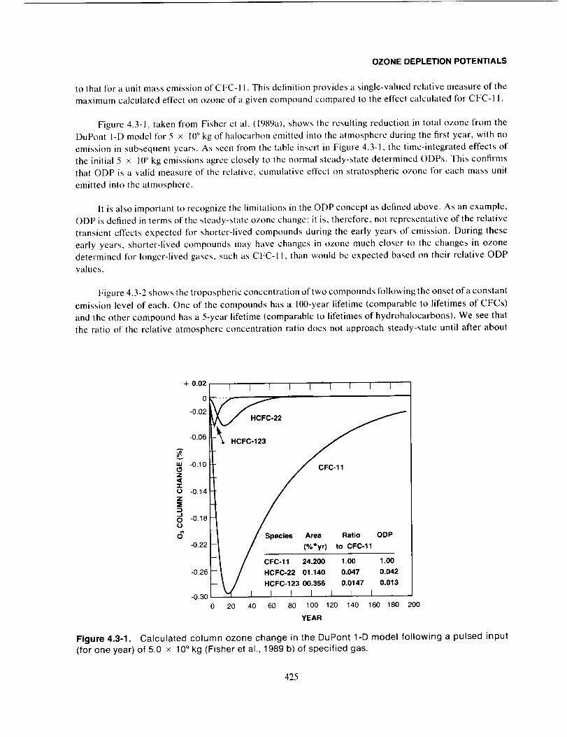
OZONE DEPLETION POTENTIALS
to that for a unit mass emission of CFC-11. This definition provides a single-valued relative measure of the
maximum calculated effect on ozone of a given compound compared to the effect calculated for CFC-I I.
Figure 4.3-1, taken from Fisher el al. (1989a), shows the resulting reduction in total ozone from the
DuPont I-D model for 5 × 10" kg of halocarbon emitted into the atmosphere during the first year, with no
emission in subsequent years. As seen from the table insert in Figure 4.3-1, the time-integrated effects of
the initial 5 x 10_ kg emissions agree closely to the normal steady-state determined ODPs. This confirms
that ODP is a valid measure of the relative, cumulative effect on stratospheric ozone for each mass unit
emitted into the atmosphere.
It is also important to recognize the limitations in the ODP concept as defined above. As an example,
ODP is defined in terms of the steady-state ozone change; it is, therefore, not representative of the relative
transient effects expected for shorter-lived compounds during the early years of emission. During these
early years, shorter-lived compounds may have changes in ozone much closer to the changes in ozone
determined for longer-lived gases, such as CFC-I I, than would be expected based on their relative ODP
values.
Figure 4.3-2 shows the tropospheric concentration of two compounds following the onset of a constant
emission level of each. One of the compounds has a 100-year lifetime (comparable to lifetimes of CFCs)
and the other compound has a 5-year lifetime (comparable to lifetimes of hydrohalocarbons). We see that
the ratio of the relative atmosphere concentration ratio does not approach steady-state until after about
4-0.0_ ... I I I I I I I 1
-0.02 _2
-0.06 II _, HCFC-123
-0.10 CFC-11
-0.14
/ .....I_ / Species Area Ratio OOP
II / 24.200 1.00 1.00--0.26 F _ / HCFC-22 01.140 0.047 0.0!2-
I- \ / .cFc-,=a00.as6 o.o147o.o,a-o.3o I _ I I I I I I I I
0 20 40 60 80 100 120 140 160 180 200
YEAR
Figure4.3-1. Calculated column ozone change in theDuPont 1-D model following a pulsed input
(for one year) of 5.0 × 10⁹ kg (Fisher et al., 1989 b) of specified gas.
425
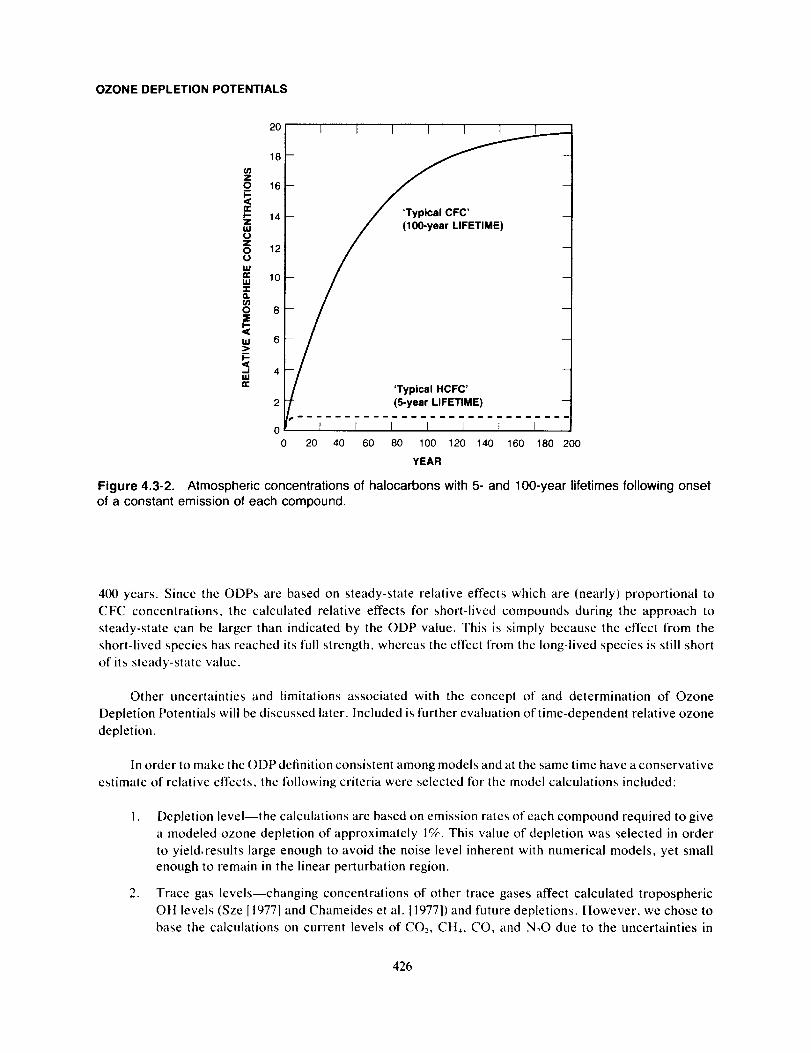
OZONE DEPLETION POTENTIALS
20
18tar)ZO 16I--<C
I-- 14ZU.ItJZO 12qJ
ILln- 10gJ-l-,.tOr)o 8=EI.--
,,, 6>_I-
IIWn,.
2
00
I I I I I I I
_
'Typical HCFC'
(5-year LIFETIME)................ m... ........
I I I l J f I
20 40 60 80 100 120 140 160 180 200
YEAR
Figure 4.3-2. Atmospheric concentrations of halocarbons with 5- and 100-year lifetimes following onset
of a constant emission of each compound.
400 years. Since the ODPs are based on steady-state relative effects which are (nearly) proportional to
CFC concentrations, the calculated relative effects for short-lived compounds during the approach to
steady-state can be larger than indicated by the ODP value. This is simply because the effect from the
short-lived species has reached its full strength, whereas the effect from the long-lived species is still short
of its steady-state value.
Other uncertainties and limitations associated with the concept of and determination of Ozone
Depletion Potentials will be discussed later. Included is further evaluation of time-dependent relative ozone
depletion.
In order to make the ODP definition consistent among models and at the same time have a conservative
estimate of relative effects, the following criteria were selected for the model calculations included:
1. Depletion level--the calculations are based on emission rates of each compound required to give
a modeled ozone depletion of approximately I%. This value of depletion was selected in order
to yield.results large enough to avoid the noise level inherent with numerical models, yet small
enough to remain in the linear perturbation region.
2. Trace gas levels--changing concentrations of other trace gases affect calculated tropospheric
OH levels (Sze [1977] and Chameides et al. [1977]) and future depletions. However, we chose to
base the calculations on current levels of CO2, CH4, CO, and N20 due to the uncertainties in
426
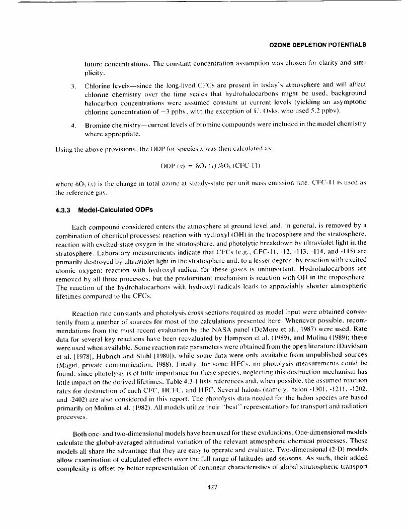
OZONE DEPLETION POTENTIALS
future concentrations. The constant concentration assumption was chosen for clarity and sim-
plicity.
3. Chlorine levels--since the long-lived CFCs are present in today's atmosphere and will affect
chlorine chemistry over the time scales that hydrohalocarbons might be used, background
halocarbon concentrations were assumed constant at current levels (yielding an asymptotic
chlorine concentration of -3 ppbv, with the exception of U. Oslo, who used 5.2 ppbv).
4. Bromine chemistry--current levels of bromine compounds were included in the model chemistry
where appropriate.
Using the above provisions, the ODP for species ._ was then calcul_ted as:
ODP (.r) = 8()_ f._)/80, (CFC-I I)
where 80_ (.v) is the change in total ozone at steady-state per unit mass emi_,sion rate. CFC-I I is used as
the reference gas.
4.3.3 Model-Calculated ODPs
Each compound considered enters the atmosphere at ground level and, in general, is removed by a
combination of chemical processes: reaction with hydroxyl (OH) in the troposphere and the stratosphere,
reaction with excited-state oxygen in the stratosphere, and photolytic breakdown by ultraviolet light in the
stratosphere. Laboratory measurements indicate that CFCs (e.g., CFC-I 1, -12, -I 13, -I 14, and -! 15) are
primarily destroyed by ultraviolet light in the stratosphere and, to a lesser degree, by reaction with excited
atomic oxygen; reaction with hydroxyl radical for these gases is unimportant. Hydrohalocarbons are
removed by all three processes, but the predominant mechanism is reaction with OH in the troposphere.
The reaction of the hydrohalocarbons with hydroxyl radicals leads to appreciably shorter atmospheric
lifetimes compared to the CFCs.
Reaction rate constants and photolysis cross sections required as model input were obtained consis-
tently from a number of sources for most of the calculations presented here. Whenever possible, recom-mendations from the most recent evaluation by the NASA panel (DeMore et al., 1987) were used. Rate
data for several key reactions have been reevaluated by Hampson et al. (1989), and Molina (1989); these
were used when available. Some reaction rate parameters were obtained from the open literature (Davidson
et al. [1978], Hubrich and Stuhl [19801), while some data were only available from unpublished sources
(Magid, private communication, 1988). Finally, for some HFCs, no photolysis measurements could be
found; since photolysis is of little importance for these species, neglecting this destruction mechanism has
little impact on the derived lifctimes. Table 4.3-1 lists references and, when possible, the assumed reaction
rates for destruction of each CFC, HCFC, and HFC. Several halons (namely, halon -1301, -121 I, -1202,
and -2402) are also considered in this report. The photolysis data needed tbr the halon species are based
primarily on Molina et al. (1982). All models utilize their "best" representations for transport and radiation
processes.
Both one- and two-dimensional models have been used for these evaluations. One-dimensional models
calculate the global-averaged altitudinal variation of the relevant atmospheric chemical processes. These
models all share the advantage that they are easy to operate and evaluate. Two-dimensional (2-D) models
allow examination of calculated effects over the full range of latitudes and seasons. As such, their added
complexity is offset by better representation of nonlinear characteristics of global stratospheric transport
427
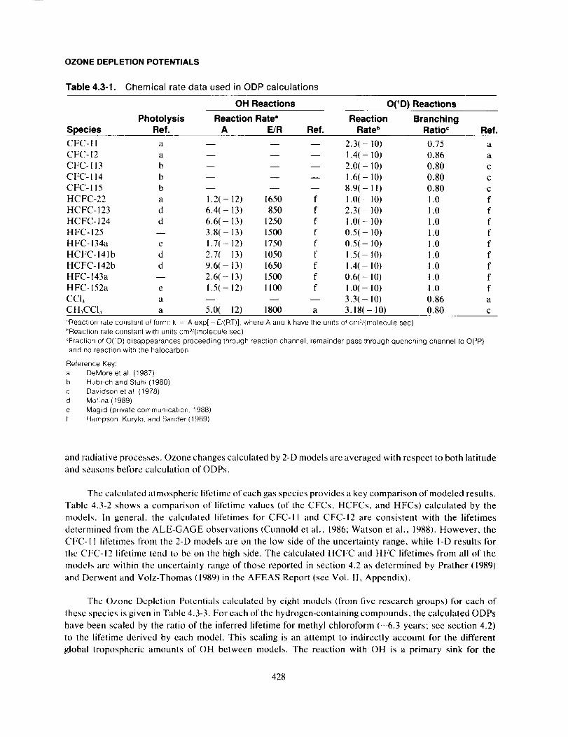
OZONE DEPLETION POTENTIALS
Table 4.3-1. Chemical rate data used in ODP calculations
OH Reactions
Photolysis Reaction Rate"
Species Ref. A E/R Ref.
O(1D) Reactions
Reaction
Rate bBranching
Ratio c Ref.
CFC-I I a -- -- -- 2.3( - !0)
CFC- 12 a -- -- -- 1.4(- 10)
CFC-113 b -- -- -- 2.0(- 10)
CFC-114 b -- -- -- 1.6( - 10)
CFC-115 b -- -- -- 8.9( - I !)
HCFC-22 a 1.2( - 12) 1650 f 1.0(- 10)
HCFC-123 d 6.4(- 13) 850 f 2.3(- 10)
HCFC-124 d 6.6(- 13) 1250 f 1.0(- 10)
HFC-125 -- 3.8(- 13) 1500 f 0.5(- 10)
HFC-134a e i.7(- 12) 1750 f 0.5(- 10)
HCFC-141b d 2.7(- 13) 1050 f 1.5(- 10)
HCFC-142b d 9.6(- 13) 1650 f 1.4(- I0)
HFC-I43a -- 2.6(- 13) 1500 f 0.6(- 10)HFC-152a e 1.5(-12) II00 f !.0(- 10)
CCI4 a -- -- -- 3.3(- 10)
CH,CCI_ a 5.0(- 12) 1800 a 3.18(- 10)
0.75
0.86
0.80
0.80
0.80
.0
.0
.0
.0
.0
.0
.0
.0
.0
0.86
0.80
JReaction rate constant of form: k = A exp[ - E/(RT)],where A and k have the units of cm3/(motecule sec).hReactionrate constant with units cm3/(molecute sec)':Fraction of O(_D)disappearances proceeding through reaction channel, remainder pass through quenching channel to O(3P)and no reaction with the halocarbon
Reference Key:a DeMore et al (1987)b Hubrich and Stuhl (1980)c Davidson et al (1978)d Motina (1989)e Magid (private communication, 1988)f Hampson, Kurylo, and Sander (1989)
and radiative processes. Ozone changes calculated by 2-D models are averaged with respect to both latitude
and seasons before calculation of ODPs.
The calculated atmospheric lifetime of each gas species provides a key comparison of modeled results.
Table 4.3-2 shows a comparison of lifetime values (of the CFCs, HCFCs, and HFCs) calculated by the
models. In general, the calcuhtted lifetimes for CFC-Ii and CFC-12 are consistent with the lifetimes
determined from the ALE-GAGE observations (Cunnold el al., 1986; Watson el al., 1988). However, the
CFC-II lifetimes from the 2-D models are on the low side of the uncertainty range, while I-D results for
the CFC-12 lifetime tend to be on the high side. The calculated HCFC and HFC lifetimes from all of the
models arc within the uncertainty range of those reported in section 4.2 as determined by Prather (1989)
and Derwent and Volz-Thomas (1989) in the AFEAS Report (see Vol. I1, Appendix).
The Ozone Depletion Potentials calculated by eight models (from five research groups) for each of
thesc specics is given in Table 4.3-3. For each of the hydrogen-containing compounds, the calculated ODPs
have been scaled by the ratio of the inferred lifetime for methyl chloroform (-6.3 years; see section 4.2)
to the lifetime derived by each model. This scaling is an attempt to indirectly account for the different
global tropospheric amounts of OH between models. The reaction with OH is a primary sink for the
428
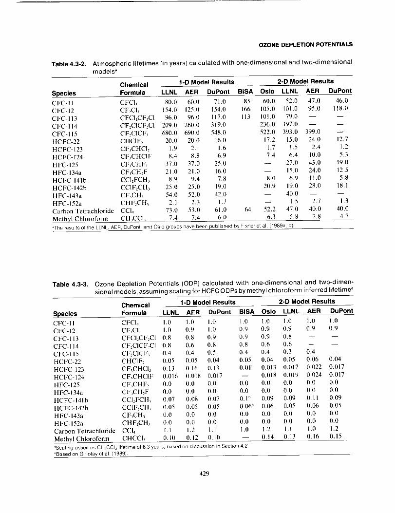
Table 4.3-2.
OZONE DEPLETION POTENTIALS
Atmospheric lifetimes (in years) calculated with one-dimensional and two-dimensionalmodels a
Chemical 1-D Model Results 2-D Model Results
Species Formula LLNL AER DuPont BISA Oslo LLNL AER DuPont
CFC-11 CFCL 80.0 60.0 71.0 85 60.0 52.0 47.0 46.0
CFC- 12 CF2CI,, 154.0 125.0 154.0 166 105.0 101.0 95.0 118.0
CFC-113 CFCI_CF2CI 96.0 96.0 117.0 113 101.0 79.0 -- --
CFC-114 CF2CICF2CI 209.0 260.0 319.0 236.0 197.0 -- --
CFC-Ii5 CF2CICF, 680.0 690.0 548.0 522.0 393.0 399.0 --
HCFC-22 CHCIF2 20.0 20.0 16.0 17.2 15.0 24.0 12.7
HCFC-123 CF3CHCI2 1.9 2.1 1.6 1.7 !.5 2.4 1.2HCFC-124 CF_CHCIF 8.4 8.8 6.9 7.4 6.4 10.0 5.3
HFC-125 CF_CHF2 37.0 37.0 25.0 -- 27.0 43.0 19.0
HFC-134a CF_CH,F 21.0 21.0 16.0 -- 15.0 24.0 12.5
HCFC-141b CCI2FCH_ 8.9 9.4 7.8 8.0 6.9 11.0 5.8
HCFC-142b CC1F,CH_ 25.0 25.0 19.0 20.9 19.0 28.0 18.1
HFC-143a CF3CH3 54.0 52.0 42.0 -- 40.0 -- --
HFC- 152a CH F2CH_ 2.1 2.3 1.7 -- 1.5 2.7 1.3
Carbon Tetrachloride CCI4 73.0 53.0 61.0 64 52.2 47.0 40.0 40.0
Methyl Chloroform CH3CCI_ 7.4 7.4 6.0 6.3 5.8 7.8 4.7
"The results of the LLNL, AER, DuPont, and Oslo groups have been published by Fisher et al. (1989a, b).
Table 4.3-3. Ozone Depletion Potentials (ODP) calculated with one-dimensional and two-dimen-
sional models, assuming scaling for HCFC ODPs by methyl chloroform inferred lifetime a
Chemical 1-D Model Results 2-D Model Results
Species Formula LLNL AER DuPont BISA Oslo LLNL AER DuPont
CFC-i I CFCI3 1.0 1.0 1.0 1.0 1.0 1.0 1.0 !.0
CFC-12 CF2C12 1.0 0.9 1.0 0.9 0.9 0.9 0.9 0.9
CFC-113 CFCI2CF2CI 0.8 0.8 0.9 0.9 0.9 0.8 -- --
CFC-114 CF:CICF2CI 0.8 0.6 0.8 0.8 0.6 0.6 -- --CFC-i 15 CF2CICF3 0.4 0.4 0.5 0.4 0.4 0.3 0.4 --
HCFC-22 CHC1F2 0.05 0.05 0.04 0.05 0.04 0.05 0.06 0.04
HCFC-123 CF3CHCI__ 0.13 0.16 0.13 0.01" 0.013 0.017 0.022 0.017
HCFC-124 CF3CHCIF 0.016 0.018 0.017 -- 0.018 0.019 0.024 0.017
HFC-125 CF_CHF_, 0.0 0.0 0.0 0.0 0.0 0.0 0.0 0.0
HFC-134a CF,CH_,F 0.0 0.0 0.0 0.0 0.0 0.0 0.0 0.0
HCFC-141 b CCI2FCH_ 0.07 0.08 0.07 0.1 h 0.09 0.09 0.11 0.09
HCFC-142b CCIF,CH_ 0.05 0.05 0.05 0.06 b 0.06 0.05 0.06 0.05
HFC-143a CF_CH3 0.0 0.0 0.0 0.0 0.0 0.0 0.0 0.0
HFC-152a CHF2CH3 0.0 0.0 0.0 0.0 0.0 0.0 0.0 0.0Carbon Tetrachloride CCI4 1.1 1.2 1.1 1.0 1.2 1.1 1.0 1.2
Methyl Chloroform CHCCL 0. I0 0.12 0.10 -- 0.14 0.13 0.16 0.15
aScaling assumes CH3CCI3 lifetime of 6.3 years, based on discussion in Section 42
bBased on Gillotay et al. (1989).
429

OZONE DEPLETION POTENTIALS
hydrogen-containing species; differences in calculated tropospheric OH concentrations account for much
of the model differences in chemical lifetimes for these gases. Therefore, amounts of OH account for much
of the variation in ODPs derived between models. However, as noted by Fisher et al. (1989a, b), using
globally averaged OH deduced from CH3CCI_ to calculate lifetimes for other HCFCs may not necessarily
be accurate, particularly for those HCFCs with lifetimes substantially different from methyl chloroform.
As seen in Table 4.3-3, the ODPs for each hydrogen-containing species, including the suggested
replacement compounds, are much smaller than those for the CFCs. This difference largely reflects the
reactivity of these species with OH, resulting in shorter chemical lifetime for the HCFCs compared to the
CFCs. Several compounds, such as HFC-134a and HCF-152a, have ODPs of zero because they do not
contain chlorine.
In general, the ODPs derived using the different models compare extremely well with each other.
However, significant differences between modeled ODPs still exist. The variation between models in the
ODP for CH_CCI3, for example, is likely related to differences in the calculated distribution of OH with
altitude and latitude between models. Although the two-dimensional models generally have a sounder
physical basis for their formulation than existing one-dimensional models, there are no significant differ-
ences between the I-D and 2-D model results.
Table 4.3-4 gives the ODPs determined by three groups (AER and LLNL I-D models and U. Oslo
2-D model) tk)r several brominated halocarbons. Although the ODPs for these compounds are shown
relative to CFC-I1 for historical reasons, the ODPs for bromine-containing compounds should in reality
be compared relative to each other because of the strong dependence to background chh)rine levels in
determining bromine effects on ozone. Therefore, in Table 4.3-4, Bromine Ozone Depletion Potentials
(BODPs) are used for relative comparisons with halon-1301, the compound with the longest lifetime and
largest ODP, as the reference. The major ozone destruction due to the halons comes from coupled chlorine-
bromine chemistry in the lower stratosphere. Because of interactions between chlorine and bromine
chemistry, the traditional ODPs are critically dependent on chlorine levels in the background atmosphere.
Also, because current models underestimate the CIO concentrations in the lower stratosphere at high
latitudes in early spring, the traditional ODP definition (relative to CFC-I I) may underestimate the true
ozone depletion potential for these compounds.
Table 4.3-4. Ozone depletions (ODPs) for brominated compounds as calculated in the AER andLLNL 1-D models and the U. Oslo 2-D model
Atmospheric Lifetime(yrs) ODP" BODP
Common Name AER LLNL Oslo AER LLNL Oslo AER LLNL Oslo
81 72
12 18halon-1301 107.0 16.0 13.2 7.8 1.0 1.0 1.0
halon-1211 15.0 3.5 2.2 3.0 0.22 0.17 0.38halon- 1202 1.5 0.3 0.02
halon-2402 28.0 23 6.2 5.0 0.5 0.64
"Relative to CFC-11, shown for historical purposes Values will be underestimates if they account for effects at polar latitudesAssumed upper stratospheric CI, mixing ratio is 3 ppbv in the LLNL and AER models and 45 ppbv in the Oslo model
"Bromine Ozone Depletion Potentials (BODPs)defined relative to halon-1301, lhe longest brominated gas.
430
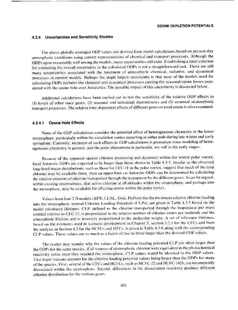
4.3.4 Uncertainties and Sensitivity Studies
OZONE DEPLETION POTENTIALS
The above globally averaged ODP values are derived from model calculations based on present-day
atmospheric conditions using current representations of chemical and transport processes. Although the
ODPs agree reasonably well among the models, many uncertainties still exist. Establishing a strict criterion
for estimating the overall uncertainty in the calculated ODPs is not a straightforward task. There are still
many uncertainties associated with the treatment of atmospheric chemical, radiative, and dynamical
processes in current models. Perhaps the single largest uncertainty is that none of the models used for
calculating ODPs includes the chemical and dynamical processes causing the seasonal ozone losses asso-
ciated with the ozone hole over Antarctica. The possible impact of this uncertainty is discussed below.
Additional calculations have been carried out to test the sensitivity of the relative ODP effects to
(I) levels of other trace gases, (2) seasonal and latitudinal dependencies and (3) assumed stratospheric
transport processes. The relative time-dependent effects of different gases on total ozone is also examined.
4.3.4.1 Ozone Hole Effects
None of the ODP calculations consider the potential effect of heterogeneous chemistry in the lower
stratosphere, particularly within the circulation vortex occurring at either pole during late winter and early
springtime. Currently, inclusion of such effects in ODP calculations is premature since modeling of heter-
ogeneous chemistry in general, and the polar phenomena in particular, are still in the early stages.
Because of the apparent special chlorine processing and dynamics within the winter polar vortex,
local Antarctic ODPs are expected to be larger than those shown in Table 4.3-3. Insofar as the observed
long-lived tracer distributions, such as those for CFC-I1 in thc polar vortex, suggcst that much of the total
chlorine may bc aw_ilable there, then an upper limit on Antarctic ODPs can be determined by calculating
the relative amounts of chlorine transported through the tropopause by the different gases. It can be argued,
within existing uncertainties, that active chlorine al all altitudes within the stratosphere, and perhaps into
the mesosphere, may be awfilable for affecting ozone within the polar vortex.
Values from four 2-D models (AER, LLNL, Oslo, DuPont) for the maximum relative chlorine loading
into the stratosphere, termed Chlorine I,oading Potentials (CLPs), are given in Table 4.3-5 based on the
model calculated lifetimes. CLP, defined as the chlorine transported through thc tropopause per mass
emitted relative to CFC-I1, is proportional to the relative number of chlorinc atoms per molecule and the
atmospheric lifetime and is inversely proportional to the molecular weight. A set of reference lifetimes,
based on the estimates used in scenario development in Chapter 3, section 3.2. I for the CFCs and from
the analysis in Section 4.2 for the HCFCs and HFCs, is given in Table 4.3-6 along with thc corresponding
CLP valucs. These values are as much as a factor of two to thrcc larger than the derived ODP wdues.
The reader may wonder why the values of the chlorine loading potential CLP are often larger than
the ODPs for the same species, lfall sources of stratospheric chlorine were equivalent in the photochemical
reactivity sense once they reached the stratospherc, CI,P values would be identical to the ODP values.
Two major reasons account for the chlorine loading potential values being larger than the ODPs for many
of the species. First, several of the CFCs and HCFCs, such as HCFC-22 and HCFC-142b, are incompletely
dissociated within the stratospherc. Second, differences in the dissociation reactivity produce different
chlorine distribution for the various gases.
431
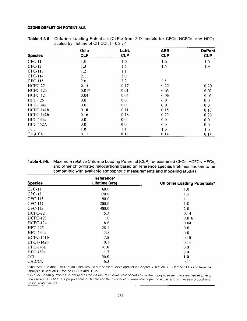
OZONE DEPLETION POTENTIALS
Table 4.3-5. Chlorine Loading Potentials (CLPs) from 2-D models for CFCs, HCFCs, and
scaled by lifetime of CH3CCI3 ( = 63 yr)
HFCs,
Oslo LLNL AER DuPont
Species CLP CLP CLP CLP
CFC- l I 1.0 1.0 ! .0 1.0CFC-12 1.3 1.5 !.5 1.9
CFC-113 1.2 l.l
CFC-114 2.1 2.0
CFC-115 2.6 2.2 2.5
HCFC-22 0.15 0.17 0.22 0.20
HCFC-123 0.017 0.01 0.03 0.02
HCFC- 124 0.04 0.04 0.06 0.05
HFC- 125 0.0 0.0 0.0 0.0
HFC-134a 0.0 0.0 0.0 0.0
HCFC-141b 0. I0 0.11 0.15 0.13
HCFC- 142b 0.16 0.18 0.22 0.20
H FC- 143a 0.0 0.0 0.0 0.0
HFC-152A 0.0 0.0 0.0 0.0
CC14 1.0 !.1 1.0 1.0CH_CCI_ 0.11 0.12 0.14 0.14
Table 4.3-6. Maximum relative Chlorine Loading Potential (CLP) for examined CFCs, HCFCs, HFCs,
and other chlorinated halocarbons based on reference species lifetimes chosen to be
compatible with available atmospheric measurements and modeling studies
Reference"
Species Lifetime (yrs) Chlorine Loading Potentials _
CFC-11 60.0 1.0
CFC-12 120.0 1.5
CFC-113 90.0 I.II
CFC-114 200.0 1.8
CFC- I 15 400.0 2.0
HCFC-22 15.3 0.14HCFC-123 1.6 0.016
HCFC- 124 6.6 0.04
H FC- 125 28.1 0.0
HFC-134a 15.5 0.0
HCFC-141b 7.8 0.10
HFCF-142b 19. I 0.14
HFC-143a 41.0 0.0
HFC-152a 1.7 0.0
CCI4 50.0 1.0
CH_CCI, 6.3 0.11
"Lifetimes (e-folding time) are on estimates used in scenario development in Chapter 3, section 3.2.1 for the CFCs and from the
analysis in Section 4.2 for the HCFCs and HFCs.
_Chlorine Loading Potential is defined as the maximum chlorine transported across the tropopause per mass emitted relative to
the same for CFC-11; it is proportional to lifetime and the number of chlorine atoms per molecule, and is inversely proportional
to molecular weight.
432
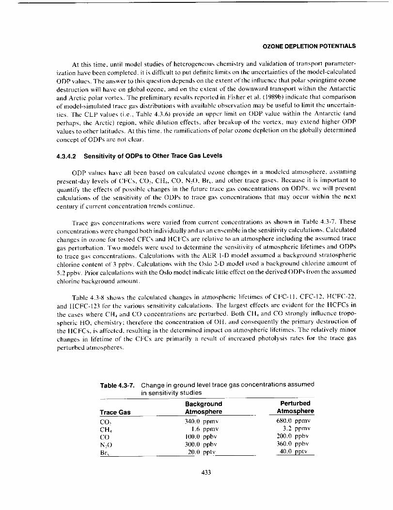
OZONE DEPLETION POTENTIALS
At this time, until model studies of heterogeneous chemistry and validation of transport parameter-
ization have been completed, it is difficult to put definite limits on the uncertainties of the model-calculated
ODP values. The answer to this question depends on the extent of the influence that polar springtime ozone
destruction will have on global ozone, and on the extent of the downward transport within the Antarctic
and Arctic polar vortex. The preliminary results reported in Fisher et al. (1989b) indicate that comparison
of model-simulated trace gas distributions with available observation may be useful to limit the uncertain-
ties. The CLP values (i.e., Table 4.3.6) provide an upper limit on ODP value within the Antarctic (and
perhaps, the Arctic) region, while dilution effects, after breakup of the vortex, may extend higher ODP
values to other latitudes. At this time, the ramifications of polar ozone depletion on the globally determined
concept of ODPs are not clear.
4.3.4.2 Sensitivity of ODPs to Other Trace Gas Levels
ODP values have all been based on calculated ozone changes in a modeled atmosphere, assuming
present-day levels of CFCs, CO2, CH+, CO, N_O, Br_, and other trace gases. Because it is important to
quantify the effects of possible changes in the future trace gas concentrations on ODPs, we will present
calculations of the sensitivity of the ODPs to trace gas concentrations that may occur within the next
century if current concentration trends continue.
Trace gas concentrations were varied from current concentrations as shown in Table 4.3-7. These
concentrations were changed both individually and as an ensemble in the sensitivity calculations. Calculated
changes in ozone for tested CFCs and HCFCs are relative to an atmosphere including the assumed trace
gas perturbation. Two models were used to determine the sensitivity of atmospheric lifetimes and ODPs
to trace gas concentrations. Calculations with the AER 1-D model assumed a background stratospheric
chlorine content of 3 ppbv. Calculations with the Oslo 2-D model used a background chlorine amount of
5.2 ppbv. Prior calculations with the Oslo model indicate little effect on the derived ODPs from the assumed
chlorine background amount.
Table 4.3-8 shows the calculated changes in atmospheric lifetimes of CFC-I 1, CFC-12, HCFC-22,
and HCFC-123 for the various sensitivity calculations. The largest effects are evident for the HCFCs in
the cases where CH+ and CO concentrations are perturbed. Both CH4 and CO strongly influence tropo-
spheric HO_ chemistry; therefore the concentration of OH, and consequently the primary destruction of
the HCFCs, is affected, resulting in the determined impact on atmospheric lifetimes. The relatively minor
changes in lifetime of the CFCs are primarily a result of increased photolysis rates for the trace gas
perturbed atmospheres.
Table 4.3-7. Change in ground level trace gas concentrations assumed
in sensitivity studies
Background Perturbed
Trace Gas Atmosphere Atmosphere
CO2 340.0 ppmv 680.0 ppmv
CH4 1.6 ppmv 3.2 ppmvCO 100.0 ppbv 200.0 ppbv
N20 300.0 ppbv 360.0 ppbv
Brx 20.0 pptv 40.0 pptv
433
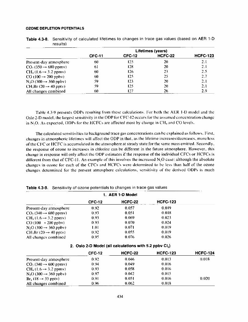
OZONE DEPLETION POTENTIALS
Table 4.3-8. Sensitivity of calculated lifetimes to changes in trace gas values (based on AER 1-D
results)
Lifetimes (years)CFC-11 CFC-12 HCFC-22 HCFC-123
Present-day atmosphere
CO, (350 _ 680 ppmv)
CH4 (I.6_ 3.2 ppmv)
CO ([00--* 200 ppbv)
N20 (300 _ 360 ppbv)
CH,Br (20 ---* 40 pptv)
All changes combined
60
61
60
60
5959
60
25 20 2. I28 20 2.1
26 23 2.5
25 25 2.723 20 2.1
25 20 2.1
27 26 2.9
Table 4.3-9 presents ODPs resulting from these calculations. For both the AER I-D model and the
Oslo 2-D model, the largest sensitivity in the ODP for CFC- 12 occurs for the assumed concentration change
in N20. As expected, ODPs for the HCFCs are affected most by change in CH4 and CO levels.
The calculated sensitivities to background trace gas concentrations can be explained as follows. First,
changes in atmospheric lifetimes will affect the ODP in that, as the lifetime increases/decreases, more/less
of the CFC or HCFC is accumulated in the atmosphere at steady state for the same mass emitted. Secondly,
the response of ozone to increases in chlorine can be different in the future atmosphere. However, this
change in response will only affect the ODP estimates if the response of the individual CFCs or HCFCs is
different from that of CFC-11. An example of this involves the increased N20 case: although the absolute
changes in ozone for each of the CFCs and HCFCs were determined to be less than half of the ozone
changes determined for the present atmosphere calculations, sensitivity of the derived ODPs is much
Table 4.3-9. Sensitivity of ozone potentials to changes in trace gas values
1. AER 1-D Model
CFC-12 HCFC-22 HCFC-123
Present-day atmosphere
CO, (340--* 680 ppmv)
CH, ( 1.6 _ 3.2 ppmv)
CO (100---* 200 ppbv)N.,O (300 _ 360 ppbv)
CH_Br (20 _ 40 pptv)
All changes combined
,
0.92 0.057 0.019
0.93 0.051 0.018
0.93 0.069 0.023
0.93 0.070 0.024
1.01 0.071 0.0190.92 0.055 0.019
0.95 0.076 0.026
Oslo 2-D Model (all calculations with 5.2 ppbv Cly)
CFC-12 HCFC-22 HCFC-123 HCFC-124
Present-day atmosphere
CO, (340 ---, 600 ppmv)CH, ( 1.6 ---, 3.2 ppmv)
N20 (300 _ 360 ppbv)
Brx (18 _ 33 pptv)
All changes combined
0.92 0.046 0.013 0.018
0.94 0.049 0.016
0.93 0.058 0.016
0.97 0.042 0.0150.91 0.051 0.016 0.020
0.96 0.062 0.018
434
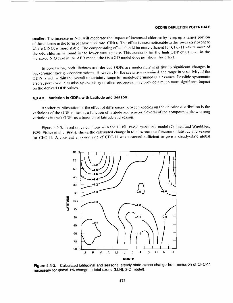
OZONE DEPLETION POTENTIALS
smaller. The increase in NOy will moderate the impact of increased chlorine by tying up a larger portion
of the chlorine in the form of chlorine nitrate, CINO,. This effect is most noticeable in the lower stratosphere
where CINO3 is more stable. The compensating effect should be more efficient for CFC-I I where more of
the odd chlorine is found in the lower stratosphere. This accounts for the high ODP of CFC-22 in the
increased N20 case in the AER model: the Oslo 2-D model does not show this effect.
In conclusion, both lifetimes and derived ODPs are moderately sensitive to significant changes in
background trace gas concentrations. However, for the scenarios examined, the range in sensitivity of the
ODPs is well within the overall uncertainty range for model-determined ODP values. Possible systematic
errors, perhaps due to missing chemistry or other processes, may provide a much more significant impact
on the derived ODP values.
4.3.4.3 Variation in ODPs with Latitude and Season
Another manifestation of the effect of differences between species on the chlorine distribution is the
variations of the ODP values as a function of latitude and season. Several of the compounds show strong
variations in their ODPs as a function of latitude and season.
Figure 4.3-3, based on calculations with the LLNI, two-dimensional model (Connell and Wuebbles,
1989: Fisher et al., 1989b), shows the calculated change in total ozone as a function of latitude and season
for CFC-11. A constant emission rate of CFC-11 was assumed sufficient to give a steady-state global
lid
I-
V-<.J
90 N[ l I I I1
75
30 -- -.
15
EQ
15
3O
45
6O
75
90 S
f--0.8
I I I 1F M A M
I I t 1 I
-1.0
-1.2 -0.8
t I I [ I IJ J A S 0 N D
MONTH
Figure 4.3-3. Calculated latitudinal and seasonal steady-state ozone change from emission of CFC-11
necessary for global 1% change in total ozone (LLNL 2-D model).
435
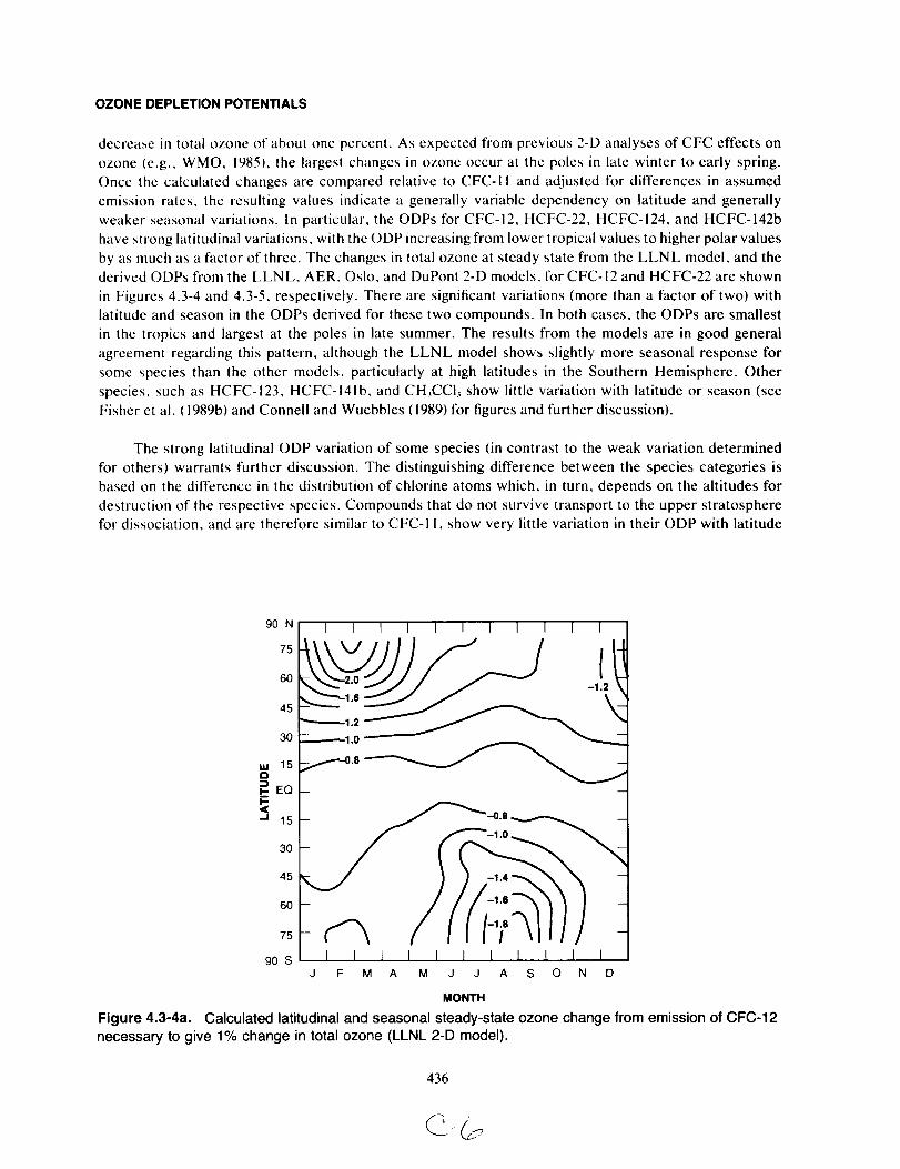
OZONE DEPLETION POTENTIALS
decrease in total ozone of about one percent. As expected from previous 2-D analyses of CFC effects on
ozone (e.g., WMO, 1985), the largest changes in ozone occur at the poles in late winter to early spring.
Once the calculated changes are compared relative to CFC-11 and adjusted for differences in assumed
emission rates, the resulting values indicate a generally variable dependency on latitude and generally
weaker seasonal variations. In particular, the ODPs for CFC-12, HCFC-22, HCFC-124, and HCFC-142b
have strong latitudinal variations, with the ODP increasing from lower tropical values to higher polar values
by as much as a factor of three. The changes in total ozone at steady state from the LLNL model, and the
derived ODPs from the LLNL, AER, Oslo, and DuPont 2-D models, for CFC-12 and HCFC-22 are shown
in Figures 4.3-4 and 4.3-5, respectively. There are significant variations (more than a factor of two) with
latitude and season in the ODPs derived for these two compounds. In both cases, the ODPs are smallest
in the tropics and largest at the poles in late summer. The results from the models are in good general
agreement regarding this pattern, although the LLNL model shows slightly more seasonal response for
some species than the other models, particularly at high latitudes in the Southern Hemisphere. Other
species, such as HCFC-123, HCFC-141b, and CH_CCI3 show little variation with latitude or season (see
Fisher et al. (1989b) and Connell and Wuebbles (1989) for figures and further discussion).
The strong latitudinal ODP variation of some species (in contrast to the weak variation determined
for others) warrants further discussion. The distinguishing difference between the species categories is
based on the difference in the distribution of chlorine atoms which, in turn, depends on the altitudes for
destruction of the respective species. Compounds that do not survive transport to the upper stratosphere
for dissociation, and are therefore similar to CFC-I I, show very little variation in their ODP with latitude
90 N| I t I I I I t I I I I
so I-1.2
30 _------1.0 -- _ _
_ EQ -
"J 15 -- -0.8 _
30
45
60
75
90 S I I I I I I I I I I IJ F M A M J J A S O N D
MONTH
Figure 4.3-4a. Calculated latitudinal and seasonal steady-state ozone change from emission of CFC-12
necessary to give 1% change in total ozone (LLNL 2-D model).
436
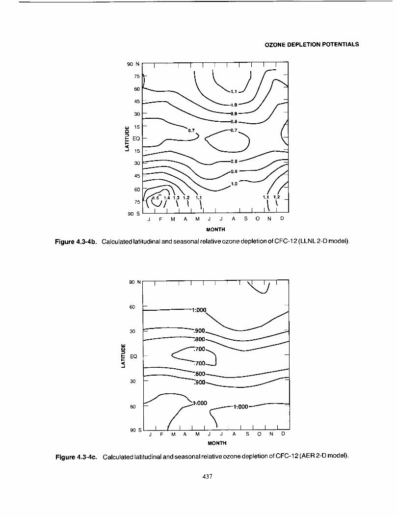
OZONE DEPLETION POTENTIALS
90 N
75
6O
45
30
m 15O,.ji- EQP
15
30
45
6O
75
9O SJ F M A M J J A S O N D
MONTH
Figure 4.3-4b. Calculated latitudinal and seasonal relative ozone depletion of CFC-1 2 (LLNL 2-D model).
90 N
60
3O
wQ
i- EQI-
.J
3O
6O
90 S
I I I I 1 I I I _ I
f
1:000_
=9oo
7oo.. _-':700..-...3
- _'_.800---..- /
_1_000 1:000_-- --f- c-"--I /I I I _ [ I 1 I I
F M A M J J A S O N D
MONTH
Figure 4.3-4¢. Calculated latitudinal and seasonal relative ozone depletion of CFC-12 (AER 2-D model).
437
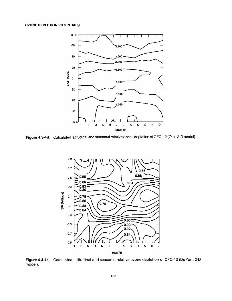
OZONE DEPLETION POTENTIALS
80 N
6O
Figure 4.3-4d.
,,iQ
P-_
J
20
2O
4O1.000
60
B0 S A S O N DJ F M A M J J
MONTH
Calculated latitudinal and seasonal relative ozone depletion of CFC-12 (Osto 2-D model).
o.9
Figure 4.3-4e.
model).
0.3
-0.5
-0.9 O N D JJ F M A M J J A S
MONTH
Calculated latitudinal and seasonal relative ozone depletion of CFC-12 (DuPont 2-D
438
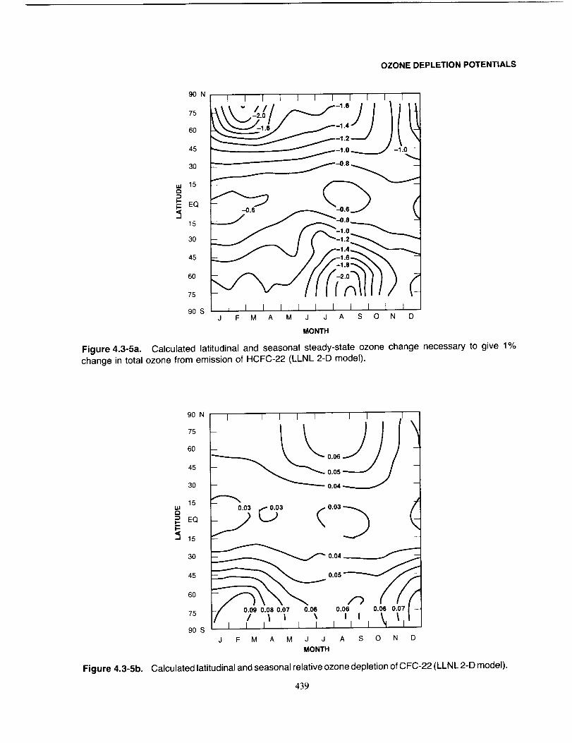
OZONE DEPLETION POTENTIALS
90 NI I I I I I i I I I I
75 -2.0
45 _ _....-.-1.0 •0
30 -- _,-.0.8
60
75
90 S [ I I I [ [ [ I I ] IJ F M A M J J A S O N D
MONTH
Figure 4.3-5a. Calculated latitudinal and seasonal steady-state ozone change necessary to give 1%change in total ozone from emission of HCFC-22 (LLNL 2-D model).
Figure 4.3-5b.
9O N
75
60
45
30
15I,LID
_ EQI-.-
30
45
60
75
90 S
1 1 I I I I I I 1 I I !
!
• /") ././@_
- , T7o?,o.o_,o.o,,,',o_o,oI.J F M A M J J A S O N D
MONTH
Calculated latitudinal and seasonal relative ozone depletion of CFC-22 (LLNL 2-D model)•
439
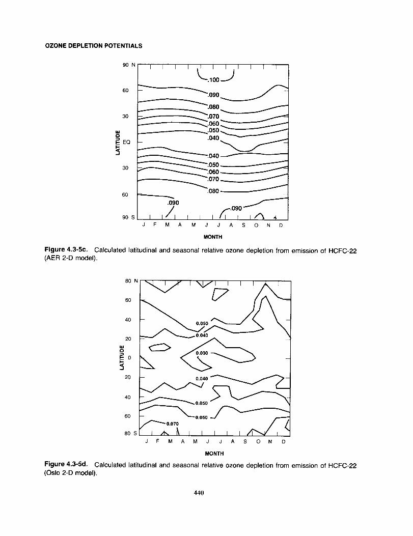
OZONE DEPLETION POTENTIALS
90 N
60
EQ
30
6O
90 S
1 I
o4o_050 -
_.o8o
.090
/ F, °J F M A M J J A S O N D
I .I 1 I I I 1 I I
L-lo0J_.090
_.080
_.o5o_-----_.040
MONTH
Figure 4.3-5c. Calculated latitudinal and seasonal relative ozone depletion from emission of HCFC-22
(AER 2-D model).
80 N
6O
4O
2O
F_°
20
40
60
80 S
r l-,q,,,,-i i I J
_ 0.050
J ,*- _ _ 1 I I 1J F M a M J J a s o N O
MONTH
Figure 4.3-5d. Calculated latitudinal and seasonal relative ozone depletion from emission of HCFC-22
(Oslo 2-D model).
440

OZONE DEPLETION POTENTIALS
0.9
0.7
0.5
0.3
'O-i
0.1
Z
-0.1
-0.3
-0.5
-0.7
-0.9J F M A M J J A S O N D J
MONTH
Figure 4.3-5e. Calculated latitudinal and seasonal relative ozone depletion from emission of HCFC-22
(DuPont 2-D model).
and season. HCFC-123 is an example of such a species. On the other hand, species that persist into the
upper stratosphere (even if the dominant removal is at lower altitudes) show strong latitudinal dependencies.
CFC-12 and HCFC-22 are two examples that show a significant latitudinal dependency. CFC-12 is primarily
dissociated at higher altitudes than CFC-il. HCFC-22, on the other hand, is primarily destroyed in the
troposphere and lower stratosphere by reaction with OH radical, yet models and observations indicate that
a significant fraction survives transport to the upper stratosphere.
The resulting strong variations of ODPs with latitude occur in response to latitudinal differences in
upper stratospheric chemistry on ozone destruction and the resultant effects of transport on both the ClOx
produced and on the ozone being destroyed. The extent of these variations depends on the treatment and
the strength of the modeled transport. It is not surprising, therefore, to find some differences in the ODP
variations with latitude and season between models. The effects of heterogeneous chemistry and polar
dynamical effects, not included in the calculations here, would lead to some modifications of these findings
but should not qualitatively change the response.
4.3.4.4 Sensitivity of ODP to Modeled Transport
The question can next be raised as to the sensitivity of ODP values to model parameters--primarily
transport processes. The treatment of transport processes is a source of significant uncertainty in 2-D
models. Changing the model transport parameters would affect the ODP directly in three ways. First, the
ODP values can change because of changes in lifetimes. The lifetime for CFC-11 is sensitive to the strength
of the circulation in the stratosphere while the lifetime of HCFC-22, which is dominated by removal in the
441
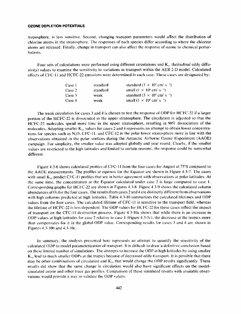
OZONE DEPLETION POTENTIALS
troposphere, is less sensitive. Second, changing transport parameters would affect the distribution of
chlorine atoms in the stratosphere. The responses of each species differ according to where the chlorine
atoms are released. Finally, change in transport can also affect the response of ozone to chemical pertur-
bations.
Four sets of calculations were performed using different circulations and Ky_ (latitudinal eddy diffu-
sivity) values to examine the sensitivity to variations in transport within the AER 2-D model. Calculated
effects of CFC-I 1 and HCFC-22 emissions were determined in each case. These cases are designated by:
Case 1 standard
Case 2 standard
Case 3 weak
Case 4 weak
standard (3 x 10 '_cm 2 s _)
small(I x 10_cm:s _)
standard (3 x 10'_cm 2 s ')
small(! x 10_cm2s -_)
The weak circulation for cases 3 and 4 is chosen to test the response of ODP for HCFC-22 if a larger
portion of the HCFC-22 is dissociated in the upper stratosphere. The circulation is adjusted so that the
HCFC-22 molecules spend more time in the upper stratosphere, resulting in 90% dissociation of the
molecules. Adopting smaller Kyy values for cases 2 and 4 represents an attempt to obtain lower concentra-
tions for species such as N20, CFC-I 1, and CFC-12 in the polar lower stratosphere more in line with the
observations obtained in the polar vortices during the Antarctic Airborne Ozone Experiment (AAOE)
campaign. For simplicity, the smaller value was adopted globally and year round. Clearly, if the smaller
values are restricted to the high latitudes and limited to certain seasons, the response could be somewhat
different.
Figure 4.3-6 shows calculated profiles of CFC- I I from the four cases for August at 75°S compared to
the AAOE measurements. The profiles at equinox for the Equator are shown in Figure 4.3-7. The cases
with small Ky_ predict CFC-I I profiles that are in better agreement with observations at polar latitudes. At
the same time, the concentration at the Equator calculated under case 2 is large compared to case I.
Corresponding graphs for HCFC-22 are shown in Figures 4.3-8. Figure 4.3-9 shows the calculated column
abundances of O, for the four cases. The results from cases 2 and 4 are distinctly different from observations
with high columns predicted at high latitudes. Table 4.3-10 summarizes the calculated lifetimes and ODP
values from the four cases. The calculated lifetime of CFC-II is sensitive to the transport field, whereas
the lifetime of HCFC-22 is less dependent. The ODP values for HCFC-22 lot these cases reflect the impact
of transport on the CFC-II destruction process. Figure 4.3-10a shows that while there is an increase in
ODP values at high latitudes for case 2 relative to case 1 (Figure 4.3-5c), the decrease at the tropics more
than compensates for it in the global ODP value. Corresponding results for cases 3 and 4 are shown in
Figures 4.3-10b and 4.3-10c.
In summary, the analysis presented here represents an attempt to quantify the sensitivity of the
calculated ODP to model parametcrization of transport. It is difficult to draw a definitive conclusion based
on these limited number of simulations. The attempts to increase the ODP at high latitudes by using smaller
K,y lead to much smaller ODPs at the tropics because of decreased eddy transport. It is possible that there
may be other combinations of circulation and K, that would change the ODP results significantly. These
results did show that the same change in circulation would also have significant effects on the model-
simulated ozone and other trace gas profiles. Comparison of these simulated results with available obser-
vations would provide a way to wdidate the ODP values.
442
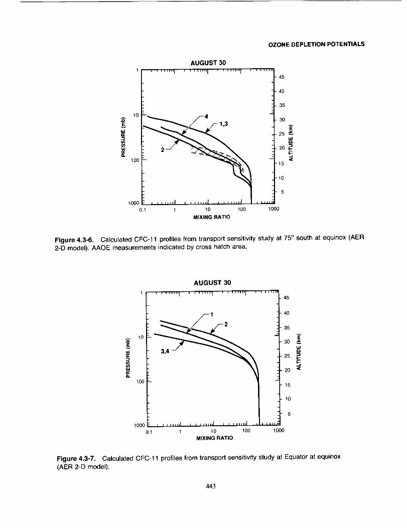
OZONE DEPLETION POTENTIALS
A 10
==,,=,==.
100
100o
AUGUST 30
........ I ........ I ........ I
o.1 1 10 lOO
MIXING RATIO
I I I IIII,
40
35
30
E25 _
Wa
_20 _F-.J
15
-10
5
I I I II
1000
Figure 4.3-6. Calculated CFC-11 profiles from transport sensitivity study at 75 ° south at equinox (AER
2-D model). AAOE measurements indicated by cross hatch area.
uJ
ct}
u.IIXa.
lO
10o
I I I IIIII I
AUGUST 30
, , ,,,,,, I l r ,l,,. I
1000 , , ,,,,,,I , , ,,,,,,I _ , ,.....I
0.1 1 10 100
MIXING RATIO
I I I I IIII
45
4O
ii i I lilt
10o0
35
A
E30
uJa
25 _F-,.J
20 '_
15
10
Figure 4.3-7. Calculated CFC-11 profiles from transport sensitivity study at Equator at equinox(AER 2-D model).
443
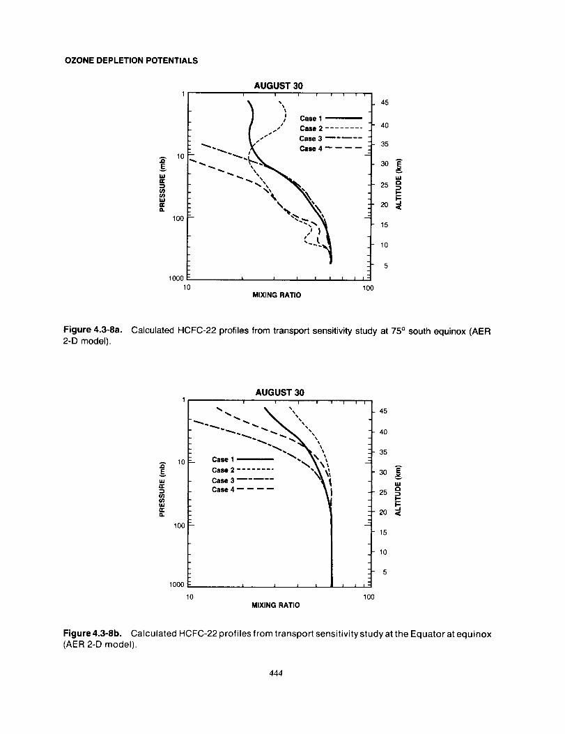
OZONE DEPLETION POTENTIALS
A 10
100
AUGUST 30
i i i i i ! i i
%%
%!t Case 1
/
,t Case 2 ........s
,f Case 3
_'_.._ _ Case 4
"\ "%
I000 I I I I I i i i
10 100MIXING RATIO
45
40
35
A30 E
Ill
25 _
eo ,_
15
10
5
Figure 4.3-8a. Calculated HCFC-22 profiles from transport sensitivity study at 75 ° south equinox (AER
2-D model).
AJ_
gILl
¢/}It}MJ
o.
10
100
1000
10
AUGUST 30
1 i i I 1
Case 1 _'.. _ \
Case 3 "_
Case 4
I l I I
MIXING RATIO
i i i
45
4O
35
25
20
15
10
5
I I I
100
30
IMa
--tl-P-.-I<
Figure 4.3-8b. Calculated HCFC-22 profiles from transport sensitivity study at the Equator at equinox
(AER 2-D model).
444
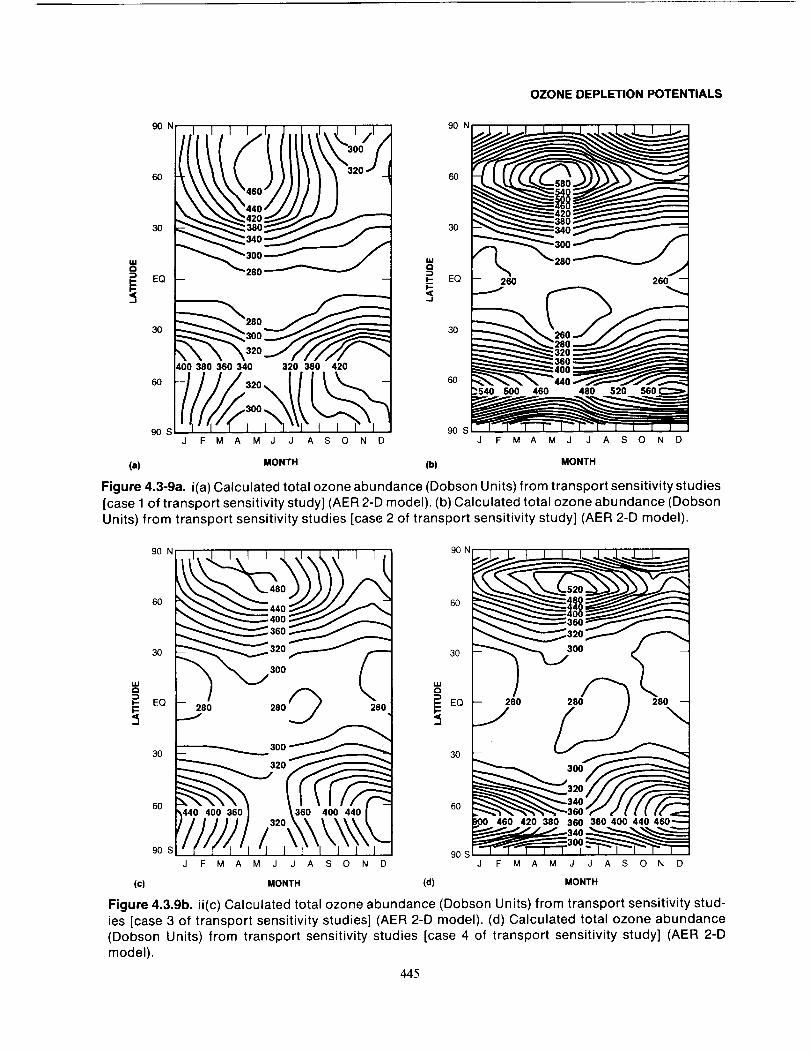
OZONE DEPLETION POTENTIALS
90N I I I I I t I X I/I 90N
_300
60 6O
3O 30
EQ -- _ EQ
30 0 _ 30
6O
9os I 9osJ F M A M J J A S O N D J F M A M J J A S O N D
(a) MONTH (b) MONTH
Figure 4.3-9a. i(a) Calculated total ozone abundance (Dobson Units) from transport sensitivity studies
[case 1 of transport sensitivity study] (AER 2-D model). (b) Calculated total ozone abundance (Dobson
Units) from transport sensitivity studies [case 2 of transport sensitivity study] (AER 2-D model).
90 NI I I I I I l -I- t ,I I 1 ,I 90N
60 _80_ 60
!iO'i'i' _ EQ
30
6090 S I 90 S
J F M A M J J A S O N D J F M A M J J A S O N D
(c) MONTH (d) MONTH
Figure 4.3,9b. ii(c) Calculated total ozone abundance (Dobson Units) from transport sensitivity stud-
ies [case 3 of transport sensitivity studies] (AER 2-D model) (d) Calculated total ozone abundance
(Dobson Units) from transport sensitivity studies [case 4 of transport sensitivity study] (AER 2-D
model)
445

OZONEDEPLETIONPOTENTIALS
Table4.3-10. Results of transport sensitivity study (AER 2-D Model) on ODP
and CLP for HCFC-22 a
Case I Case 2 Case 3 Case 4
CFC- 11 lifetime 47 years 34 years 51 years 44 years
HCFC-22 lifetime 24 years 22 years 24 years 23 years
ODP 0.07 0.035 0.055 0.034
CLP 0.27 0.35 0.25 0.28
ffhese calculations do not include the CH:_CCt3 lifetime scaling included in Table 4.3-3.
90NI I I I I.'
oo•
30 fO.02
uJa
EQ -<,.I
3O
60
90S
(a)
O.13
J F M A M J J A S O N D
MONTH
Figure 4.3-10a. Calculated latitudinal and seasonal relative ozone depletion from emission of HCFC-22 [case
2 of transport sensitivity study] (AER 2-D model).
446
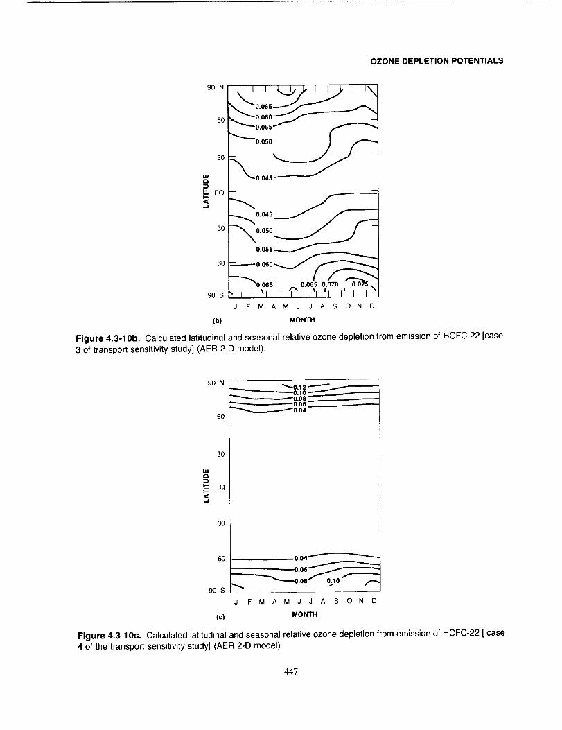
OZONE DEPLETION POTENTIALS
90 N
6O
3O
W
I-.- EQI,,-
,,-I
30
6O
90 S
_..0'045 _
,,-_o,o_,'_o,,op,,;o,_,IF M A M J J A S O N D
(b) MONTH
Figure 4.3-10b. Calculated latitudinal and seasonal relative ozone depletion from emission of HCFC-22 [case
3 of transport sensitivity study] (AER 2-D model).
90 N
60
30
UJ
i.- EQI-
,-I
•......__ _0.12 _ '
__.______o:_o__---.-----0.06 -- ""
_o.o4
90 S
30 ______60 0.04
__ ,0.06
J F M A M J J A S O N D
(c) MONTH
Figure 4.3-10c. Calculated latitudinal and seasonal relative ozone depletion from emission of HCFC-22 [ case4 of the transportsensitivitystudy] (AER 2-D model).
447
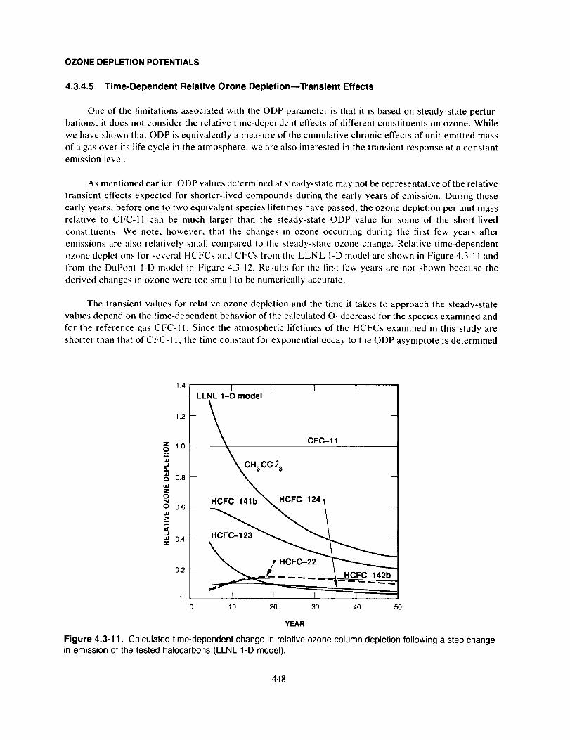
OZONE DEPLETION POTENTIALS
4.3.4.5 Time-Dependent Relative Ozone Depletion--Transient Effects
One of the limitations associated with the ODP parameter is that it is based on steady-state pertur-
bations: it does not consider the relative time-dependent effects of different constituents on ozone. While
we have shown that ODP is equivalently a measure of the cumulative chronic effects of unit-emitted mass
of a gas over its life cycle in the atmosphere, we are also interested in the transient response at a constant
emission level.
As mentioned earlier, ODP values determined at steady-state may not be representative of the relative
transient effects expected for shorter-lived compounds during the early years of emission. During these
early years, before one to two equivalent species lifetimes have passed, the ozone depletion per unit mass
relative to CFC-II can be much larger than the steady-state ODP value for some of the short-lived
constituents. We note, however, that the changes in ozone occurring during the first few years after
emissions are also relatively small compared to the steady-state ozone change. Relative time-dependent
ozone depletions for several HCFCs and CFCs from the LLNL I-D model are shown in Figure 4.3-11 and
from the DuPont I-D model in Figure 4.3-12. Results for the first few years are not shown because the
derived changes in ozone were too small to be numerically accurate.
The transient values for relative ozone depletion and the time it takes to approach the steady-state
values depend on the time-dependent behavior of the calculated Ot decrease for the species examined and
for the reference gas CFC-I I. Since the atmospheric lifetimes of the HCFCs examined in this study are
shorter than that of CFC-11, the time constant for exponential decay to the ODP asymptote is determined
p-_J.Ja.
ZoN
o
I--
W
0,i0.2
0
0 10 20 30 40 50
YEAR
Figure 4.3-11. Calculated time-dependent change in relative ozone column depletion following a step change
in emission of the tested halocarbons (LLNL 1-D model).
448
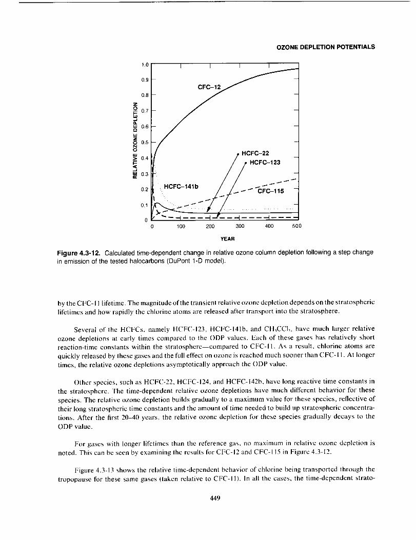
OZONE DEPLETION POTENTIALS
Z
ouJ-IQ.u.Ia
IJJZONOuJ>
,-II.Un,-
1.0
0.9
0.8
0.7
0.6
0.5
0,4
0.3
0.2
0.1
0
0
CFC-12
HCFC-22
HCFC-123
.... t -- -'( --
100 200 300 400 500
YEAR
Figure 4.3-12. Calculated time-dependent change in relative ozone column depletion following a step changein emission of the tested halocarbons (DuPont 1-D model).
by the CFC-I I lifetime. The magnitude of the transient relative ozone depletion depends on the stratospheric
lifetimes and how rapidly the chlorine atoms are released after transport into the stratosphere.
Several of the HCFCs, namely HCFC-123, HCFC-141b, and CH_CCI,, have much larger relative
ozone depletions at early times compared to the ODP values. Each of these gases has relatively short
reaction-time constants within the stratosphere--compared to CFC-I 1. As a result, chlorine atoms are
quickly released by these gases and the full effect on ozone is reached much sooner than CFC-I 1. At longer
times, the relative ozone depletions asymptotically approach the ODP value.
Other species, such as HCFC-22, HCFC-124, and HCFC-142b, have long reactive time constants in
the stratosphere. The time-dependent relative ozone depletions have much different behavior for these
species. The relative ozone depletion builds gradually to a maximum value for these species, reflective of
their long stratospheric time constants and the amount of time needed to build up stratospheric concentra-
tions. After the first 20-40 years, the relative ozone depletion for these species gradually decays to the
ODP value.
For gases with longer lifetimes than the reference gas, no maximum in relative ozone depletion is
noted. This can be seen by examining the results for CFC-12 and CFC-115 in Figure 4.3-12.
Figure 4.3-13 shows the relative time-dependent behavior of chlorine being transported through the
tropopause for these same gases (taken relative to CFC-II). In all the cases, the time-dependent strato-
449
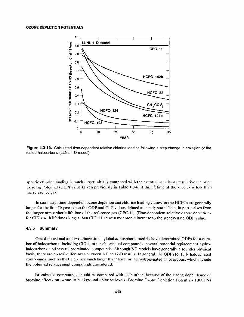
OZONE DEPLETION POTENTIALS
0.9m
08
0.7
06
05
0.4
03
02
01
I I I ILLNL 1-D model
CFC-11
-_
HCFC-141 b
- HCF P-_'"''__v,.v -___ -
I I I 1
0 10 20 30 40 50
YEAR
Figure 4.3-13. Calculated time-dependent relative chlorine loading following a step change in emission of the
tested halocarbons (LLNL 1-D model).
spheric chlorine loading is much larger initially compared with the eventual steady-state relative Chlorine
Loading Potential (CLP) value (given previously in Table 4.3-6) if the lifetime of the species is less than
the reference gas.
In summary, time-dependent ozone depletion and chlorine loading values for the HCFCs are generally
larger for the first 50 years than the ODP and CLP values defined at steady state. This, in part, arises from
the longer atmospheric lifetime of the reference gas (CFC-11). Time-dependent relative ozone depletions
for CFCs with lifetimes longer than CFC-I I show a monotonic increase to the steady-state ODP value.
4.3.5 Summary
One-dimensionaJ and two-dimensional global atmospheric models have determined ODPs for a num-
ber of halocarbons, including CFCs, other chlorinated compounds, several potential replacement hydro-
halocarbons, and several brominated compounds. Although 2-D models have generally a sounder physical
basis, there are no real differences between I-D and 2-D results. In general, the ODPs for fully halogenated
compounds, such as the CFCs, are much larger than those for the hydrogenated halocarbons, which include
the potential replacement compounds considered.
Brominated compounds should be compared with each other, because of the strong dependence of
bromine effects on ozone to background chlorine levels. Bromine Ozone Depletion Potentials (BODPs)
450

OZONE DEPLETION POTENTIALS
are used for relative comparisons with Halon-1301, which has the longest lifetime and largest ODP, as the
reference.
Although the calculated ODPs agree reasonably well among models, many uncertainties still exist.
None of the models used for calculating ODPs include the chemical and dynamical processes causing the
seasonal ozone losses over Antarctica. Another uncertainty lies in the model-calculated OH, which is a
major source of uncertainty for both lifetimes and ODPs of the HCFCs.
Because of the apparent special chlorine processing and dynamics within the winter polar vortex,
local Antarctic ODPs are expected to be larger than those derived. Insofar as the observed long-lived tracer
distributions, such as CFC- I I in the polar vortex, suggest that much of the total chlorine may be available
there, then an upper limit on Antarctic ODPs can be determined by calculating the relative amounts of
chlorine transported through the tropopause by the different gases. These CLPs determined using assumed
reference lifetimes (which generally agree with those in the models used here) can be as large as a factor
of two to three times the derived ODP values. The ramifications of polar ozone depletion for global ODPs
are not currently clear.
The time-dependent relative ozone depletion values differ from the steady-state ODP values. The
time-dependent values depend on the atmospheric lifetime and the transport time to the region of destruction
of the gas. The shorter the stratospheric lifetime, the sooner the gas will impact stratospheric ozone and
hence the higher the transient relative ozone depletion. For example, HCFC-123 has a shorter lifetime than
CFC-11; its relative ozone depletion is largest soon after emission. Other gases in this category include
HCFC-141b and CH3CCI3. Species such as HCFC-22, HCFC-124, and HCFC-142b have somewhat longer
time constants in the stratosphere. Their relative ozone depletions build slowly to values (based on their
time constants) as large as 0.2 and then decay slowly with time to the derived steady-state ODP value.
Relative ozone depletion values for HCFCs are greater than ODP values even after 30 to 50 years. Time-
dependent relative ozone depletions for CFCs with lifetimes longer than CFC- I I show a monotonic increase
to the ODP value. The ODP is the cumulative response; as discussed above, the transient response of
relative ozone depletion may be larger than the ODP value at early times after emission.
Several of the halocarbons indicate a strong latitude dependence in their ODP values and a generally
weaker seasonal variation. In particular, ODPs for species such as CFC-12, HCFC-22, HCFC-124, and
HCFC-142b, which have stratospheric loss patterns very different from CFC-11, produce strong latitudinal
gradients in ODPs, with the largest ODPs near summer poles and smallest values in the tropics. The effects
of heterogeneous chemistry and polar dynamical effects could modify these findings.
Sensitivity analyses indicate that ODPs are affected to only a minor degree (-< 20%) by assumed
variations in background levels of N,O, CH4, CO_,, CO, total stratospheric chlorine, and total stratospheric
bromine.
4.4 HALOCARBON GLOBAL WARMING POTENTIALS
4.4.1 Background
The radiative perturbations and potential climatic effects due to the infrared absorption properties of
chlorofluorocarbons (CFC-11 and CFC-12) have been assessed in WMO (1985). That assessment and those
from accompanying studies (Wang and Molnar, 1985; Owens et al., 1985; Ramanathan et al., 1985, 1987;
451
OZONE DEPLETION POTENTIALS
Fisher et al., 1989c) demonstrated that the direct radiative forcing (i.e., one in which all parameters are
held fixed while the concentration of any CFCs is increased from 0 to 1 ppbv), consists of an increase in
the downward longwave flux at the surface (surface radiative forcing) and a decrease in the net upward
flux at the tropopause (surface-troposphere net radiative forcing). This imbalance results in a net increase
in the amount of Iongwave radiation trapped within the Earth's atmosphere system, thereby potentially
enhancing the greenhouse effect.
Since the 1985 reports, infrared spectral absorption data of several halogenated compounds have
become available (Magid, private communication, 1988 and Gehring, private communication, 1988) which
not only include CFCs, but also include HFCs and HCFCs. Interest in the latter two classes of compounds
stems from their role as potential replacement compounds for CFCs. Laboratory measurements show that
all the halogenated compounds possess significant absorption in the 500-1400 cm-' ('_window") region.
The absorption spectrum for any of these species typically is one of individual lines spaced very closely
together in an arbitrary frequency interval giving the appearance of a continuum structure. The absorption
cross sections of the HFCs and HCFCs also occur at similar frequencies in the "window" region and are
comparable in magnitude to those for CFCs.
Because the absorption bands of all replacement halogenated compounds fall in the infrared "window"
region, the potential greenhouse effects need to be assessed. This need is emphasized by the fact that the
clear portions of the Earth's atmosphere have virtually no other constituents (excepting aerosols) with
major absorption bands in the "window" region. In overcast conditions, clouds also have absorption bands
in this region. Furthermore, the Earth's outward-going radiation is at a maximum near the "window"
region for the Earth's surface temperatures. Therefore, the presence of halogenated compounds could play
an important part in determining the radiation balance in the clear portion of the atmosphere and a non-
negligible role in the overcast portions.
Besides the influence on the infrared radiative fluxes, there is yet another aspect of the perturbations
by the halogenated compounds, as pointed out in WMO (1985). This is the heating perturbations induced
in the upper troposphere and lower stratosphere which, owing to the large radiative time constant of those
regions of the atmosphere, have the potential to increase the temperatures there. Any change in the
temperatures near the tropopause region is of potential significance for the tropospheric-stratospheric
exchange of water vapor.
The effectiveness of greenhouse gases is accentuated by their lifetimes and in large part by their
corresponding atmospheric abundances.
In this report, we consider the most recently available laboratory spectral data of the halogenated
compounds and assess the following:
• the direct radiative forcing due to the halogenated compounds, as evaluated by both line-by-line
(GFDL) and band models (AER, DuPont),
• the changes in the surface temperature, as evaluated by the one-dimensional radiative-convective
models (AER, DuPont), and
• the relative changes in the surface temperatures taking into account the chemical lifetimes of the
compounds expressed as Greenhouse Warming Potentials.
452
OZONE DEPLETION POTENTIALS
The GFDL line-by-line radiative transfer model has been developed from that described in Schwarz-
kopf and Fels (1989). The band models employed in the AER and DuPont algorithms have been described
earlier (Wang and Molnar, 1985; Owens et al., 1985). The absorption cross sections of the halogenated
compounds are incorporated in a manner similar to the water vapor continuum. It should be noted that in
the absence of a temperature-dependent dataset, none of these algorithms incorporate temperature depen-
dence in calculated radiative effects.
No attempt is made to calculate Greenhouse Warming Potentials for non-halocarbon gases such as
carbon dioxide and methane. Due to their current atmospheric concentrations and the spectral locations
of their infrared absorption bands, calculated global warming is not proportional to atmospheric concen-
tration changes of these gases. In contrast, calculated warmings are linearly proportional to halocarbon
concentrations.
4.4.2 Definition of Halocarbon GWP
Halocarbon Global Warming Potential (Halocarbon GWP) is defined parallel to the Ozone Depletion
Potential. It is defined as the ratio of steady-state calculated warming for each unit mass of a gas emitted
into the atmosphere (as indicated by the change in infrared flux at the tropopause) relative to the calculated
warming for a mass unit of reference gas CFC-I 1. This definition was chosen as a representative measure
of the potential of a compound to effect global warming, since:
1. It provides a measure of the cumulative effect on the radiative balance over its chemical lifetime
for each unit released into the atmosphere (see below).
2. The Halocarbon GWP yields a single value for each compound rather than a time-varying
multitude of values.
3. It provides a measure of the maximum calculated effect of a compound compared to the maximum
calculated effect ofCFC-I 1 on an equal mass basis.
The first reason is perhaps the most important in that it estimates the cumulative effect on potential
global warming of each unit released. An illustrative test was performed which quantified the chronic effect
from a single pulsed release of test gas into the atmosphere. This particular test used the DuPont model to
calculate cumulative global warmings over a 500-year time period following emissions of HCFC- 123, HCFC-
22, and CFC-t I.
The calculated cumulative warmings are shown in Figure 4.4- I. For each case, the modeled warming
is maximum very soon after the release and exponentially decays with a time constant equal to the
atmospheric lifetime of the species. As seen in the insert table, the time-integrated warmings echo the
relative values of the Halocarbon GWP calculated from steady-state figures.
In order to make the definition of Halocarbon GWP consistent between models as well as a conser-
vative estimate of relative effects, the following criteria have been selected:
I, Trace gas levels--Changing the concentration of other trace gases could affect the calculated
future equilibrium temperature rise from gases under evaluation here for two reasons. First, if
there is overlap of absorption spectra, certain frequency bands would have less effect. Secondly,
chemistry and therefore lifetime can be affected by perturbation of these chemicals. Current
levels of CO2, CH4, N20, 03, and stratospheric H20 were used in model calculations.
453
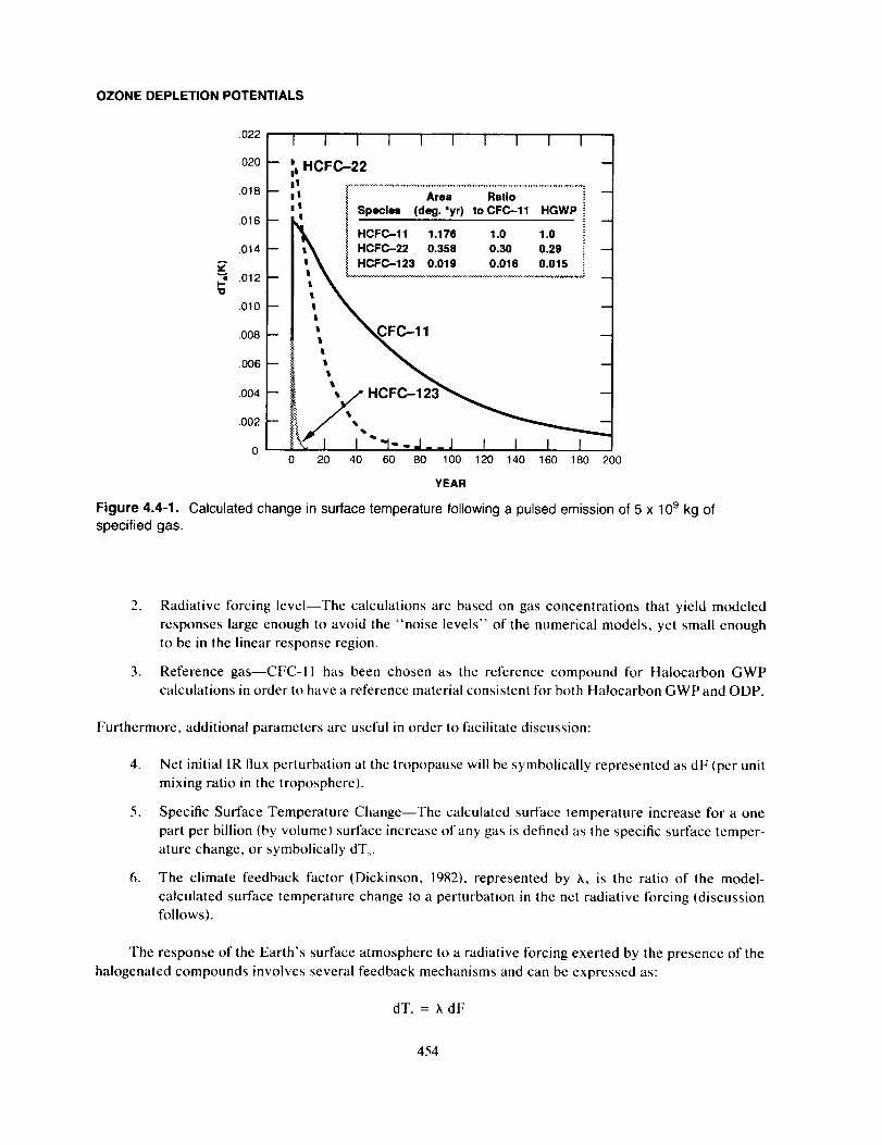
OZONE DEPLETION POTENTIALS
A
iiI--'O
.022
.020
.018
.016 --
.014 --
.012 --
.010 --
.008 --
.006 --
.004 t.002
0
I I I
-- _1 HCFC-22
I I I I I 1 I
I !
1 Area Ratio --
I Speclea (d,_eg.'yr_._))IoCFC.- HGW.___P
I HCFC-11 1.176 1.0 1.0 --
I_ { HCFC-22 0.358 0.30 0.29 --I _, _ HCFC-123 O 019 0016 0 015
II HCFHCFC-123
0 20 40 60 80 100 t20 140 160 180 200
YEAR
Figure 4.4-1. Calculated change in surface temperature following a pulsed emission of 5 x 10 9 kg of
specified gas.
,
.
Radiative forcing level--The calculations are based on gas concentrations that yield modeled
responses large enough to avoid the "noise levels" of the numerical models, yet small enough
to be in the linear response region.
Reference gas--CFC-II has been chosen as the reference compound for Halocarbon GWP
calculations in order to have a reference material consistent for both Halocarbon GWP and ODP.
Furthermore, additional parameters are useful in order to facilitate discussion:
4. Net initial IR flux perturbation at the tropopause will be symbolically represented as dF (per unit
mixing ratio in the troposphere).
5. Specific Surface Temperature Change--The calculated surface temperature increase for a one
part per billion (by volume) surface increase of any gas is defined as the specific surface temper-
ature change, or symbolically dT,.
6. The climate feedback factor (Dickinson, 1982), represented by k, is the ratio of the model-
calculated surface temperature change to a perturbation in the net radiative forcing (discussion
follows).
The response of the Earth's surface atmosphere to a radiative forcing exerted by the presence of the
halogenated compounds involves several feedback mechanisms and can be expressed as:
dT_ = hdF
454
OZONE DEPLETION POTENTIALS
where dT_ is a measure of the climate response. The factor h depends on mechanisms not all of which are
quantitatively understood. Nevertheless, as stated in WMO (1985), h can be expected to be in the range of
0.25-1 K/W m 2. Studies surveyed by Ramanathan et al. (1985) have two values ranging from 0.47-0.53,
while the DuPont and AER models have a h of 0.64, and 0.81, respectively. It must be realized that the
range in h stated above is not a rigid bracketing. Two important aspects of climate modeling severely
restrict our present ability to better quantify h precisely. One is the lack of understanding of the response
of the ocean circulation and the ensuing effects on the atmosphere. The second is the lack of knowledge
of the changes in the cloud amounts and cloud properties due to changes in the halocarbon radiative forcing.
Our knowledge in both the areas needs to improve substantially in order to better quantify h.
The Halocarbon GWP definition resembles the ODP definition. For any gas, the general definition is:
Halocarbon GWP =
Calculated IR forcing due to compound X/
Emission rate (steady state) of compound X
Calculated IR forcing due to CFC-I I/
Emission rate (steady state) of CFC-11
Note, since lifetimes are proportional to the ratio of atmospheric abundance to (molecular weight *
emission rate), an equivalent form of this definition is:
Halocarbon GWP =[dF(x) * Lifetime(x) / Molecular weight(x)]
[dF(CFC- 1 I) * Lifetime(CFC- I I ) / Molecular weight(CFC- 11)]
(This formula has been used to calculate Halocarbon GWP from the line-by-line radiative model results.)
Since radiative-convective models calculate a change in surface temperature, it is useful to express
an equivalent form of the Halocarbon GWP, assuming the same value of h for all gases, as:
Halocarbon GWP =[dTs(x) * Lifetime(x) / Molecular weight(x)]
[dTs(CFC-11 ) * Lifetime(CFC- I 1) / Molecular weight(CFC- ! I)]
Note also, many of these gases have the potential of affecting heating rates indirectly as well, since they
can chemically influence the distribution of ozone. Examination of model results indicates that this is a
second order effect, at least two orders of magnitude below the 1R effect and well below the sensitivity of
these calculations (Wang et al., 1989).
4.4.3 Model-Calculated Halocarbon GWPs
A primary input to these radiative calculations are the altitudinal steady-state concentration profiles
which are calculated using appropriate chemistry models.
After the concentration profile is determined, the effect of each gas is calculated using a radiative
model. This calculation accounts for the amount of energy absorbed by each IR gas over the radiation
spectrum and accounts for the spectral overlap with other IR active gases. Quantitative infrared data for
this input are available (see Fisher et al., 1989c).
Table 4.4-1 shows the net IR radiative flux at the tropopause (=12 km) for a 1 ppbv tropospheric
mixing ratio, as calculated by each of the three models. Note that each of the model's calculations was
455
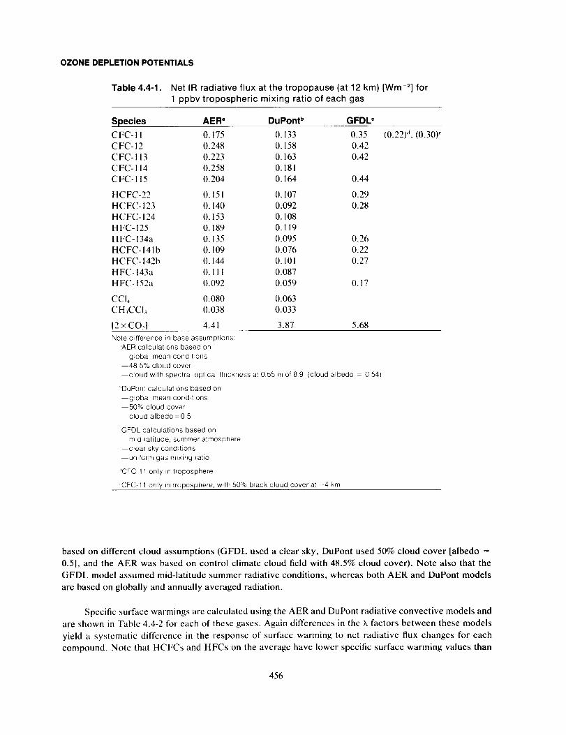
OZONE DEPLETION POTENTIALS
Table 4.4-1. Net IR radiative flux at the tropopause (at 12 km) [Wm 2] for
1 ppbv tropospheric mixing ratio of each gas
Species AER ° DuPont b GFDL c
CFC-I 1 0.175 0.133 0.35 (0.22) d, (0.30) _
CFC-12 0.248 0.158 0.42
CFC- 113 0.223 0.163 0.42
CFC-114 0.258 0.181
CFC-115 0.204 0.164 0.44
HCFC-22 0.151 0.107 0.29
HCFC- 123 0.140 0.092 0.28
HCFC-124 0.153 0.108
HFC-125 0.189 0.119
HFC- 134a 0.135 0.095 0.26
HCFC-141b 0.109 0.076 0.22
HCFC- 142b 0.144 0.101 0.27
HFC-143a 0. I 11 0.087
HFC- 152a 0.092 0.059 0.17
CCL 0.080 0.063
CH_CCI_ 0.038 0.033
12 × CO_,] 4.41 3.87 5.68
Note difference in base assumptions:'AER calculations based on
--global mean conditions--485% cloud cover
cloud with spectral optical thickness at 055 m of 89 (cloud albedo 054)
_'DuPont calculations based on
--global mean conditions--50% cloud cover
cloud albedo 0.5
' GFDL calculations based on
mid-latitude, summer atmosphere--clear sky conditions--uniform gas mixing ratio
'_CFC-t 1 only in troposphere
"CFC-11 only in troposphere, with 50% black cloud cover at _--4km
based on different cloud assumptions (GFDL used a clear sky, DuPont used 50% cloud cover [albedo =
0.51, and the AER was based on control climate cloud field with 48.5% cloud cover). Note also that the
GFDL model assumed mid-latitude summer radiative conditions, whereas both AER and DuPont models
are based on globally and annually averaged radiation.
Specific surface warmings are calculated using the AER and DuPont radiative convective models and
are shown in Table 4.4-2 tbr each of these gases. Again differences in the h factors between these models
yield a systematic difference in the response of surface warming to net radiative flux changes for each
compound. Note that HCFCs and HFCs on the average have lower specific surface warming values than
456
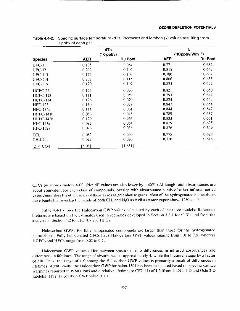
Table 4.4-2.
OZONE DEPLETION POTENTIALS
Specific surface temperature (dTs) increases and lambda (,k) values resulting from
1 ppbv of each gas
Species
dTs h
(°K/ppbv) (°K/ppbv/Wm- =)AER Du Pont AER Du Pont
CFC-I I 0. 135 0.084 0.771 0.632
CFC-12 0.202 0.102 0.815 0.647
CFC-113 0.174 0.103 0.780 0.632
CFC-114 0.208 0.115 0.806 0.635
CFC-115 0.170 0.107 0.833 0.652
HCFC-22 0.124 0.070 0.821 0.650
HCFC-123 0. I I I 0.059 0.793 0.644
HCFC- 124 0.126 0.070 0.824 0.645
HFC- 125 0.160 0.078 0.847 0.654
HFC- 134a 0. 114 0.061 0.844 0.647
HCFC- 141 b 0.086 0.048 0.789 0.637
HCFC- 142b 0.120 0.066 0.833 0.651
HFC- 143a 0.092 0.054 0.829 0.625
HFC- ! 52a 0.076 0.038 0.826 0.649
CCI4 0.062 0.040 0.775 0.628
C H_CCI_ 0.027 0.020 0.710 0.618
12 x CO2] [3.08] ll.6511
CFCs by approximately 40%. (Net dF values are also lower by -40%.) Although total absorptances are
about equivalent for each class of compounds, overlap with absorptance bands of other infrared active
gases diminishes the efficiencies of these gases as greenhouse gases. Most of the hydrogenated halocarbons
have bands that overlap the bands of both CH4 and N20 as well as water vapor above 1250 cm-_.
Table 4.4-3 shows the Halocarbon GWP values calculated by each of the three models. Reference
lifetimes are based on the estimates used in scenarios developed in Section 3.3.1 for CFCs and from the
analysis in Section 4.2 for HCFCs and HFCs.
Halocarbon GWPs for fully halogenated compounds are larger than those for the hydrogenated
halocarbons. Fully halogenated CFCs have Halocarbon GWP values ranging from 1.0 to 7.5, whereas
HCFCs and HFCs range from 0.02 to 0.7.
Halocarbon GWP values differ between species due to differences in infrared absorbances and
differences in lifetimes. The range of absorbances is approximately 4, while the lifetimes range by a factor
of 250. Thus, the range of 400 among the Halocarbon GWP values is primarily a result of differences in
lifetimes. Additionally, the Halocarbon GWP for halon-1301 has been calculated based on specific surface
warmings reported in WMO 1985 and a relative lifetime (to CFC-I 1) of 1.3 (from LLNL I-D and Oslo 2-D
models). This Halocarbon GWP value is 1.4.
457
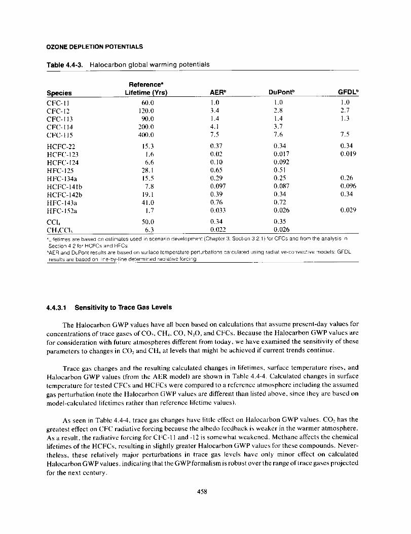
OZONE DEPLETION POTENTIALS
Table 4.4°3. Halocarbon global warming potentials
Reference"
Species Lifetime (Yrs) AER b DuPonP GFDL b
CFC- I 1 60.0 1.0 1.0 1.0
CFC-12 120.0 3.4 2.8 2.7
CFC-113 90.0 1.4 1.4 1.3
CFC-114 200.0 4. I 3.7
CFC- 115 400.0 7.5 7.6 7.5
HCFC-22 15.3 0.37 0.34 0.34
HCFC-123 1.6 0.02 0.017 0.019
HCFC- 124 6.6 0. I0 0.092
HFC- 125 28.1 0.65 0.5 IHFC-134a 15.5 0.29 0.25 0.26
HCFC- 141 b 7.8 0.097 0.087 0.096
HCFC- ! 42b 19.1 0.39 0.34 0.34
HFC-143a 41.0 0.76 0.72
HFC-152a 1.7 0.033 0.026 0.029
CCIa 50.0 0.34 0.35CH3CCIs 6.3 0.022 0.026
"Lifetimes are based on estimates used in scenario development (Chapter 3, Section 3.2 1) for CFCs and from the analysis inSection 4.2 for HCFCs and HFCs,
t_AERand DuPont results are based on surface temperature perturbations calculated using radiative-convective models; GFDLresults are based on line-by-line determined radiative forcing.
4.4.3.1 Sensitivity to Trace Gas Levels
The Halocarbon GWP values have all been based on calculations that assume present-day values for
concentrations of trace gases of CO__, CH4, CO, N20, and CFCs. Because the Halocarbon GWP values are
for consideration with future atmospheres different from today, we have examined the sensitivity of these
parameters to changes in CO., and CH4 at levels that might be achieved if current trends continue.
Trace gas changes and the resulting calculated changes in lifetimes, surface temperature rises, and
Halocarbon GWP values (from the AER model) are shown in Table 4.4-4. Calculated changes in surface
temperature for tested CFCs and HCFCs were compared to a reference atmosphere including the assumed
gas perturbation (note the Halocarbon GWP values are different than listed above, since they are based on
model-calculated lifetimes rather than reference lifetime values).
As seen in Table 4.4-4, trace gas changes have little effect on Halocarbon GWP values. CO_, has the
greatest effect on CFC radiative forcing because the albedo feedback is weaker in the warmer atmosphere.
As a result, the radiative forcing for CFC-I l and -12 is somewhat weakened. Methane affects the chemical
lifetimes of the HCFCs, resulting in slightly greater Halocarbon GWP values for these compounds. Never-
theless, these relatively major perturbations in trace gas levels have only minor effect on calculated
Halocarbon GWP values, indicating that the GWP formalism is robust over the range of trace gases projected
for the next century.
458
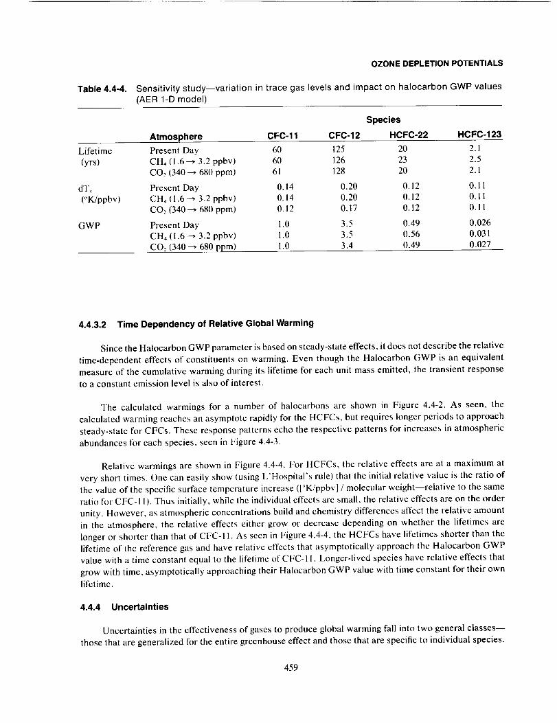
Table 4.4-4.
OZONE DEPLETION POTENTIALS
Sensitivity study--variation in trace gas levels and impact on halocarbon GWP values
(AER 1-D model)
Species
Atmosphere CFC-11 CFC-12 HCFC-22 HCFC-123
Lifetime Present Day 60 125 20 2. I
(yrs) CH4 (1.6 _ 3.2 ppbv) 60 126 23 2.5
CO, (340 _ 680 ppm) 61 128 20 2.1
dT_ Present Day 0.14 0.20 0.12 0.11
(°K/ppbv) CH4 (1.6---_ 3.2 ppbv) 0.14 0.20 0.12 0.11CO,, (340 _ 680 ppm) 0. ! 2 0.17 0.12 0.11
GWP Present Day 1.0 3.5 0.49 0.026
CH4 (i .6---_ 3.2 ppbv) 1.0 3.5 0.56 0.031
CO2 (340 _ 680 ppm) 1.0 3.4 0.49 0.027
4.4.3.2 Time Dependency of Relative Global Warming
Since the Halocarbon GWP parameter is based on steady-state effects, it does not describe the relative
time-dependent effects of constituents on warming. Even though the Halocarbon GWP is an equivalent
measure of the cumulative warming during its lifetime for each unit mass emitted, the transient response
to a constant emission level is also of interest.
The calculated warmings for a number of halocarbons are shown in Figure 4.4-2. As seen, the
calculated warming reaches an asymptote rapidly for the HCFCs, but requires longer periods to approach
steady-state for CFCs. These response patterns echo the respective patterns for increases in atmospheric
abundances for each species, seen in Figure 4.4-3.
Relative warmings are shown in Figure 4.4-4. For HCFCs, the relative effects are at a maximum at
very short times. One can easily show (using L'Hospital's rule) that the initial relative value is the ratio of
the value of the specific surface temperature increase (l°K/ppbv] / molecular weight--relative to the same
ratio for CFC-I I). Thus initially, while the individual effects are small, the relative effects are on the order
unity. However, as atmospheric concentrations build and chemistry differences affect the relative amount
in the atmosphere, the relative effects either grow or decrease depending on whether the lifetimes are
longer or shorter than that of CFC-1 I. As seen in Figure 4.4-4, the HCFCs have lifetimes shorter than the
lifetime of the reference gas and have relative effects that asymptotically approach the Halocarbon GWP
value with a time constant equal to the lifetime of CFC-I 1. Longer-lived species have relative effects that
grow with time, asymptotically approaching their Halocarbon GWP value with time constant for their own
lifetime.
4.4.4 Uncertainties
Uncertainties in the effectiveness of gases to produce global warming fall into two general classes--
those that are generalized for the entire greenhouse effect and those that are specific to individual species.
459
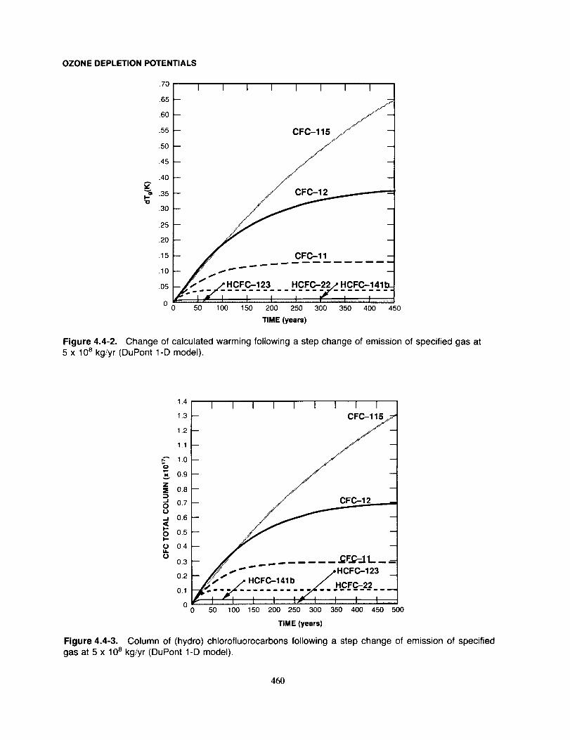
OZONE DEPLETION POTENTIALS
.70
.65
.60
.55
.50
.45
.40
.35
.30
.25
.20
.15
.10
.05
0
I I I I I 1 I I
-- CFC-115 /f" -
- jJ -
----- .o.J_ CFC-12 _._-
0 50 100 150 200 250 300 350 400 450
TIME (years)
Figure 4.4-2. Change of calculated warming following a step change of emission of specified gas at
5 x 10⁸ kg/yr (DuPont 1-D model).
1.4 I I I I I I I I I
1.3 -- CF_j_
1_1 J
0
_ 0.9
Z
•J 0.70
,,I 0.6<I,-0 0.5
o 0.4I,I.
0.1 ' "',_= ........ . _,(_' " " _' " 'o _ I r I I ___1...........1_ ; l I I .........
0 50 100 150 200 250 300 350 400 450 500
TIME (years)
Figure 4,4-3, Column of (hydro) chlorofluorocarbons following a step change of emission of specified
gas at 5 x 10⁸ kg/yr (DuPont 1-D model).
46O
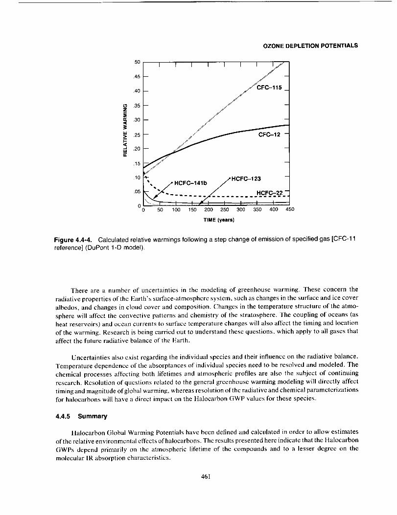
Oz
I.IJ
>V---I
ne
OZONE DEPLETION POTENTIALS
5O
,45
.40
.35
.30
.25
.20
.15
.10
.05
00
I I I I I I I _"f
-- f_" --
_ .J_CFC-115 _
-- /_ ,/./,J_'_
'"".._ .... I I _ I 1 I .......... I ', I50 100 150 200 250 300 350 400 450
TIME (years)
Figure 4.4-4. Calculated relative warmings following a step change of emission of specified gas [CFC-11
reference] (DuPont 1-D model).
There are a number of uncertainties in the modeling of greenhouse warming. These concern the
radiative properties of the Earth's surface-atmosphere system, such as changes in the surface and ice cover
albedos, and changes in cloud cover and composition. Changes in the temperature structure of the atmo-
sphere will affect the convective patterns and chemistry of the stratosphere. The coupling of oceans (as
heat reservoirs) and ocean currents to surface temperature changes will also affect the timing and location
of the warming. Research is being carried out to understand these questions, which apply to all gases that
affect the future radiative balance of the Earth.
Uncertainties also exist regarding the individual species and their influence on the radiative balance.
Temperature dependence of the absorptances of individual species need to be resolved and modeled. The
chemical processes affecting both lifetimes and atmospheric profiles are also the subject of continuing
research. Resolution of questions related to the general greenhouse warming modeling will directly affect
timing and magnitude of global warming, whereas resolution of the radiative and chemical parameterizations
for halocarbons will have a direct impact on the Halocarbon GWP values for these species.
4.4.5 Summary
Halocarbon Global Warming Potentials have been defined and calculated in order to allow estimates
of the relative environmental effects ofhalocarbons. The results presented here indicate that the Halocarbon
GWPs depend primarily on the atmospheric lifetime of the compounds and to a lesser degree on the
molecular IR absorption characteristics.
461
OZONE DEPLETION POTENTIALS
The reduction in Halocarbon GWP that might be expected due to use replacement of a CFC by a
hydrohalocarbon can be estimated by taking the ratio of the Halocarbon GWP of the hydrohalocarbon to
the Halocarbon GWP of the CFC it would replace. For example, the reduction in Halocarbon GWP in
replacing uses of CFC-12 by HCFC-134a is (0.26 _ 0.030)/(3.07) = 0.085 _+ 0.01. Of course, the relative
quantities of the compound required in the use application must also be taken into account.
Although the Halocarbon GWP values reported here agree reasonably well among models, uncer-
tainties in the values still exist because of the uncertainties in modeled chemistry and dynamics and their
direct effect on the chemical lifetimes of these compounds.
Halocarbon GWP values appear to be reasonably robust parameters since their calculated values are
nearly insensitive to assumed concentrations of other radiative gases. The minor shifting of the Halocarbon
GWP values is primarily influenced by the changes in calculated lifetimes and therefore the abundance in
the atmosphere.
Calculated time-dependent relative global warmings for Halocarbons are initially on order unity but
decrease or increase depending on whether their lifetimes are shorter or longer than that of the reference
gas. At longer times, the relative global warmings asymptotically approach the Halocarbon GWP values.
REFERENCES
Blake, D. R., and F. S. Rowland, Continuing worldwide increase in tropospheric methane, 1978 to 1987,
Science, 239, 1129-1131, 1988.
Bojkov, R. D., Surface ozone during the second half of the nineteenth century, J. Climate and Appl.
Meteor., 25,343-352, 1986.
Chameides, W. L., and J. C. G. Walker, A photochemical theory of tropospheric ozone, J. Geophys.
Res., 78, 8751-8760, 1973.
Chameides, W. L., S. C. Liu, and R. C. Cicerone, Possible variations in atmospheric methane, J. Geophys.
Res., 82, 1795-1798, 1977.
Connell, P. S., and D. J Wuebbles, _'Evaluating CFC Alternatives From the Atmospheric Viewpoint, "Air
and Waste Management Association paper 89-5.7, 1989; also Lawrence Livermore National Labo-
ratory report UCRL-99927 Rev. 1, 1989.
Cox, R. A., and R. G. Derwent, Gas phase chemistry of the minor constituents of the troposphere, in
Specialist Periodic" Report Gas Kinetics and Energy Transfer, Vol. 4, The Royal Society of Chemistry,
London, pp. 189-232, 1981.
Crutzen, P. J., A discussion of the chemistry of some minor constituents of the stratosphere and tropo-
sphere, Pure and Applied Geophys, 106-108, 1385-1399, 1973.
Crutzen, P. J., Photochemical reactions initiated by and influencing ozone in unpolluted tropospheric air,
Tellus, 26, 47-57, 1974.
Crutzen, P. J., Tropospheric ozone: An overview, in Tropospheric Ozone: Regional and Global Scale
Interactions, edited by 1. S. A. lsaksen, NATO ASI Series C, D. Reidel, Dordrecht, 1988.
Crutzen, P. J., and C. Bruhl, The impact of observed changes in atmospheric chemistry and climate, in
The Environmental Record in Glaciers and h'e Sheets, edited by H. Oeschger and C. C. Langway,
Jr., Wiley, New York, pp. 249-266, 1989.
Crutzen, P. J., and J. Fishman, Average concentrations of OH in the troposphere, and the budgets of CH4,
CO, CH 3CCi3, Geophys. Res. Lett., 4, 321-324, 1977.
462
OZONE DEPLETION POTENTIALS
Cunnold, D. M., R. G. Prinn, R. A. Rasmussen, P. G. Simmonds, F. N. Alyea, C. A. Cardelino, A. J.
Crawford, P. J. Fraser, and R. D. Rosen, Atmospheric lifetime and annual release estimates for CCi3F
and CCI2F2 from five years for ALE data, J. Geophys. Res., 91, 10797-10817, 1986.
Davidson, J. A., H. 1. Schiff, T. J. Brown, and C. J. Howard, Temperature dependence of the rate constants
for reactions of O(JD) atoms with a number of halocarbons, J. Chem. Phys., 69, 4277-4279, 1978.
DeMore, W. B., M. J. Molina, S. P. Sander, D. M. Golden, R. F. Hampson, M. J. Kurylo, C. J. Howard,
and A. R. Ravishankara, Chemical Kinetics and Photochemical Data.['or Use in Stratospheric
Modeling, JPL Publication 87-41, pp. 196, Jet Propulsion Laboratory, Pasadena, CA, 1987.
Derwent, R. G., and A. R. Curtis, "Two-Dimensional Model Studies of Some Trace Gases and Free
Radicals in the Troposphere," AERE report R8853, H.M. Stationery Office, London, 1977.
Derwent, R. G., and A. E. J. Eggleton, Two-dimensional model studies of methyl chloroform in the
troposphere, Quart. J. Roy. Met. Soc., 107, 231-242, 1981.
Derwent, R., and A. Volz-Thomas, The tropospheric lifetime of halocarbons and their reactions with OH
radicals: an assessment based on the concentration of _4CO, in Alternative Fluorocarbons Environ-
mental Acceptability Study (AFEAS), Vol. II, Appendix, this report (1990), 1989.
Dickinson, R. E., Modeling climatic changes due to carbon dioxide increases, in Carbon Dioxide Review,
edited by W.C. Clark, pp. 101-133, Clarendon Press, New York, 1982.
Dorn, H. P., J. Callies, U. Platt, and D. H. Ehhalt, Measurement of tropospheric OH concentrations by
laser long-path absorption spectroscopy, Tellus, 40B, 437-445, 1988.
Ehhalt, D. H., How has the atmospheric concentration of CH4 changed? in The Changing Atmosphere,
edited by F. S. Rowland and I. S. A. Isaksen, Wiley-Interscience, New York, pp. 25-32, 1988.
Ehhalt, D. H., and J. Rudolph, On the importance of light hydrocarbons in multiphase atmospheric systems,
Ber. Kernforschungsanlage, Julich, West Germany, JUL-1942, pp. 1-43, 1984.
Fahey, D. W., G. Hubler, D. D. Parrish, E. J. Williams, R. B. Norton, B. A. Ridley, H. C. Singh, S. C.
Liu, and F. C. Fehsenfeld, Reactive nitrogen species in the troposphere: Measurements of NO, NOz,
HNO3, particulate nitrate, peroxyacetyl nitrate (PAN), O3, and total reactive odd nitrogen (NOy) at
Niwot Ridge, Colorado, J. Geophys. Res., 91, 9781-9793, 1986.
Fehsenfeld, F. C., D. D. Parrish, and D. W. Fahey, The measurement of NO_ in the non-urban troposphere,
in Tropospheric Ozone: Regional and Global Scale Interactions, edited by. I. S. A. Isaksen, NATO
AS1 Series C, D. Reidel, Dordrecht, 1988.
Fisher, D. A., C. H. Hales, D. L. Filkin, M. K. W. Ko, D. N. Sze, P. S. Connell, D. J. Wuebbles, I. S.
A. Isaksen, and F. Stordal, Ozone depletion potentials for CFCs and possible replacements, submitted
to Nature, 1989a.
Fisher, D. A., C. H. Hales, D. L. Filkin, M. K. W. Ko, N. D. Sze, P. S. Connell, D. J. Wuebbles, I. S.
A. Isaksen, and F. Stordal, Relative effects on stratospheric ozone of halogenated methanes and
ethanes of social and industrial interest, in Alternative Fluoroearbons Environmental Acceptability
Study (AFEAS), Vol. II, Appendix, this report (1990), 1989b.
Fisher, D. A., C. H. Hales, W. C. Wang, K. W. Ko, and N. D. Sze, Relative effects of global warming of
halogenated methanes and ethanes of social and industrial interest, in Alternative Fluorocarbons
Environmental Acceptability Study (AFEAS), Vol. II, Appendix, this report (1990), 1989c.
Fishman, J., and P. J. Crutzen, The origin of ozone in the troposphere, Nature, 274,855-858, 1978.
Fraser, P. J., P. Hyson, R. A. Rasmussen, A. J. Crawford, and M. A. K. Khalil, Methane, carbon monoxide
and methyl chloroform in the southern hemisphere, J. Atmos. Chem., 4, 3-42, 1986.
Gillotay, G., P. C. Simon, and G. Brasseur, Absorption cross section of alternative chlorofluoroethanes
and potential effects on the ozone layer, Plant Space Sci., in press 1989.
Golombek, A., and R. G. Prinn, A global three-dimensional model of the circulation and chemistry of
CFCI3, CF3CI._, CH3CCI_, CC14 and NzO, J. Geophys. Res., 91, 3985-4001, 1986.
463
OZONE DEPLETION POTENTIALS
Hampson, R. F., Kurylo, M. J., and Sander, S. P., Evaluated rate constants for selected HCFC's and
HFC's with OH and O(JD), in Alternative Fluorocarbons Environmental Acceptability Study (AFEAS),
Vol. 1I, Appendix, this report (1990), 1989.
Hammitt, J. K., F. Camm, P. S. Connell, W. E. Mooz, K. A. Wolf, D. J. Wuebbles, and A. Bemazai,
Future emission scenarios for chemicals that may deplete stratospheric ozone, Nature, 330, 711-716,
1987.
Hubrich, C., and F. Stuhl, The ultraviolet absorption of some halogenated methanes and ethanes for
atmospheric interest, J. Photochem., 12, 93-107, 1980.
lsaksen, I. S. A., Tropospheric ozone budget and possible man-made effects, in Quadrennial International
Ozone Symposium, Vol. I1, edited by. J. London, pp. 845-852, IAMAP, NCAR, Boulder, Colorado,1981.
lsaksen, 1. S. A., and O. Hov, Calculation of trends in the tropospheric concentrations of O3, OH, CO,
CH4 and NO, Tellus, 39B, 271-285, 1987.
IUPAC:R. Atkinson, D. L. Baulch, R. A. Cox, R. F. Hampson Jr., J. A. Kerr, and J. Troe, Evaluated
kinetic and photochemical data for atmospheric chemistry, Suppl. II1, J. Phys. Chem. Ref. Data,1989.
Khalil, M. A. K., and R. A. Rasmussen, The atmospheric lifetime of methyl chloroform, Tellus, 36B, 317-
332, 1984.
Levy 11, H., Normal atmosphere: Large radical and formaldehyde concentrations predicted, Science, 173,
141-143, 1971.
Levy I1, H., J. D. Mahlman, and W. J. Moxim, A stratospheric source of reactive nitrogen in the unpolluted
troposphere, Geophys. Res. Lett., 7, 441-444, 1980.
Levy 11, H., J. D. Mahlman, W. J. Moxim, and S. C. Liu, Tropospheric ozone: The role of transport., J.
Geophys. Res., 90, 3753-3772, 1985.
Liu, S. C., Group report on oxidizing capacity of the atmosphere, in The Changing Atmosphere, edited
by. F. S. Rowland and I. S. A. Isaksen, Wiley lnterscience, New York, pp. 219-232, 1988.
Liu, S. C., and M. Trainer, Tropospheric ozone response to column ozone change, J. Atmos. Chem., 6,
221-223, 1987.
Logan, J. A., Tropospheric ozone: Seasonal behavior, trends and anthropogenic influence. J. Geophys.Res., 90. 10463-10482, 1985.
Logan, J. A., M. J. Prather, S. C. Wofsy, and M. B. McElroy, Tropospheric chemistry: A global perspec-
tive, J. Geophys. Res., 86, 7210-7254, 1981.
Lovelock, J. E., Methyl chloroform in the troposphere as an indicator of OH radical abundance, Nature,
267, 32-33, 1977.
Makide, Y., and F. S. Rowland, Tropospheric concentrations of methyl chloroform, CH3CCi_, in January
1978 and estimates of atmospheric residence times for hydrocarbons, Proc. Natl. Acad. Sei., USA,
5933-5937, 1981.
McConnell, J. C., and H. 1. Schiff, Methyl chloroform: Impact on stratospheric ozone, Science, 199, 174-
177, 1978.
McKay, C., M. Pandow, and R. Wolfgang, On the chemistry of natural radio-carbon, J. Geophys. Res.,
68, 3829-3931, 1963.
Midgeley, P. N., The production and release to the atmosphere of I,l,l-trichloroethane (methyl chloro-
form), Atm. Env., in press, 1989.
Molina, M. J., Review of ultraviolet absorption cross sections of a series of alternative fluorocarbons, in
Alternative Fluorocarbons Environmental Acceptability Study (AFEAS), Vol. II, Appendix, this
report (1990), 1989.
Molina, L. T., M. J. Molina, and F. S. Rowland, Ultraviolet absorption cross sections of several brominated
methanes and ethanes of atmospheric interest, J. Phys. Chem., 86, 2672-2675, 1982.
464
OZONE DEPLETION POTENTIALS
Morel, O., R. Simonaitis, and J. Heicklen, Ultraviolet absorption spectra of HOzNO2, CC1302NO_,, CCI2FO2NO2
and CH302NO2, Chem. Phys. Lett., 73, 38-42, 1980.
NASA:W. B. DeMore, S. P. Sander, M. J. Molina, D. M. Golden, R. F. Hampson, M. J. Kurylo, C. J.
Howard, and A. R. Ravishankara, Chemical Kinetics and and Photochemical Data for Use in
Stratospheric Modeling, NASA Panel for Data Evaluation, Evaluation No. 8, JPL, Publication 87-
41, Jet Propulsion Laboratory, Pasadena, CA, 1987.
Neely, W., and J. Plonka, Estimation of time-averaged hydroxyl radical concentrations in the troposphere,
Environ. Sci. Tech., 12, 317-321, 1978.
Neftel, A., J. Beer, H. Oeschger, and F. Zurcher, Sulphate and nitrate concentrations in snow from south
Greenland, Nature, 314, 611-613, 1985.
Niki, H., An assessment of potential impact of alternative fluorocarbons on tropospheric ozone, in Alter-
native Fluorocarbons Environmental Acceptability Study (AFEAS), Vol. II, Appendix, this report
(1990), 1989.
Owens, A. J., C. H. Hales, D. L. Filkin, C. Miller, J. M. Steed, and J. P. Jesson, A coupled one-dimensional
radiative-convective, chemistry transport model of the atmosphere, J. Geophys. Res., 90, 2283-2311,
! 985.
Perner, D., U. Platt, M. Trainer, G. Huebler, J. W. Drummond, W. Junkermann, J. Rudolph, B. Schubert,
A. Volz, D. H. Ehhalt, K. J. Rumpel, and G. Helas, Tropospheric OH concentrations: A comparison
of field data with model predictions, J. Atmos. Chem., 5, 185-216, 1987.
Platt, U., M. Rateike, W. Junkermann, J. Rudolph, and D. H. Ehhalt, New tropospheric OH measurements,
J. Geophys. Res., 93, 5159-5166, 1988.
Prather, M. J., Tropospheric hydroxyl concentrations and the lifetimes of hydrochlorofluorocarbons (HCFCs),
in Alternative Fluorocarbons Environmental Acceptability Study (AFEAS), Vol. II, Appendix, this
report (1990), 1989.
Prinn, R. G., R. A. Rasmussen, P. G. Simmonds, F. N. Alyea, D. M. Cunnold, B. C. Lane, C. A. Cardelino,
and A. J. Crawford, The atmospheric lifetime experiments, 5, results for CH3CCI3 based on three
years of data, J. Geophys. Res., 88, 8415-8426, 1983.
Prinn, R. G., D. Cunnold, R. A. Rasmussen, P. Simmonds, F. Alyea, A. J. Crawford, P. Fraser, and R.
Rosen, Atmospheric trends in methyl chloroform and the global average for the hydroxyl radical,
Science, 238, 945-950, 1987.
Ramanathan, V., R. J. Cicerone, H. B. Singh, and J. T. Kiehl, Trace gas trends and their potential role in
climate change, J. Geophys. Res., 90, 5547-5566, 1985.
Ramanathan, V., L. Callis, R. Cess, J. Hansen, I. Isaksen, W. Huhn, A. Lacis, F. Luther, J. Mahlman,
R. Reck, and M. Schlesinger, Climate-chemical interactions and effects of changing atmospheric
trace gases, Rev. Geophys., 25, 1441-1482, 1987.
Rasmussen, R. A., and M. A. K. Khalil, Isoprene over the Amazon basin, J. Geophys. Res., 93, 1417-
1421, 1988.
Rognerud, B., I. S. A. lsaksen, and F. Stordal, Model studies of stratospheric ozone depletion, Proceedings
of the Quadrennial Ozone Symposium, Gottingen, F.R.G., edited by R. D. Bojkov and P. Fabian,
Deepak Publications, Hampton, VA., 1988.
Rudolph, J., Two-dimensional distribution of light hydrocarbons:Results from the STRATOZ lII experi-
ment, J. Geophys. Res., 93, 8367-8377, 1988.
Schwarzkopf, M. D., and S. B. Fels, The simplified exchange method revised: An accurate rapid method
for computation of IR cooling rates, J. Geophys. Res., in press, 1989.
Singh, H. B., Atmospheric halocarbons: Evidence in favour of reducing average hydroxyl radical concen-
tration in the troposphere, Geophys. Res. Lett., 4, 101-104, [977a.
Singh, H. B., Preliminary estimates of average tropospheric OH concentrations in the northern and southern
hemispheres, Geophys. Res. Lett., 4,453-456, 1977b.
465
OZONE DEPLETION POTENTIALS
Singh, H. B., and J. F. Kasting, Chlorine-hydrocarbon photochemistry in the marine troposphere and
lower stratosphere, J. Atmos. Chem., 7, 261-285, 1988.
Singh, H. B., L. J. Salas, and R. E. Stiles, Selected man-made halogenated chemicals in the air and oceanic
environment, J. Geophys. Res., 88, 3675-3683, 1983.
Singh, H. B., L. J. Salas, and W. Viezee, The global distribution of peroxyacetyl nitrate, Nature, 321,
588-591, 1986.
Sze, N. D., Anthropogenic CO emissions: Implications for the atmospheric CO-OH-CH4 cycle, Science,
195, 673, 1977.
Thompson A. M., R. W. Stewart, M. A. Owens, and J. A. Heruche, Sensitivity of tropospheric oxidants
to global chemical and climate change, Atmos. Environ., 23,519-532, 1989.
United Nations Environment Programme., Montreal Protocol on Substances that Deplete the Ozone
Layer--Final Act., UNEP, Nairobi, Kenya, 1987.
Volz, A., D. H. Ehhalt, and R. G. Derwent, Seasonal and latitudinal variation in _4CO and the tropospheric
concentration of hydroxyl radicals, J. Geophys. Res., 86, 5163-517 I, 1981.
Wang, W.-C., and G. Molnar, A model study of the greenhouse effects due to increasing CH4 N20, CFECIE
and CFCI3, J. Geophys. Res., 90, 12971-12980, 1985.
Wang, W.-C., G. Molnar, M. K. W. Ko, S. Goldenberg, and N. D. Sze, Atmospheric trace gas and global
climate: A seasonal study, Tellus, in press, 1989.
Warneck, P., On the role of OH and HO2 radicals in the troposphere, Tellus, 26, 39-46, 1974.
Warneck, P., Production rates of OH in the troposphere, Planet. Space Sci., 23, 1507-1518, 1975.
Watson, R. T. and Ozone Trends Panel, Prather, M. J. and Ad Hoc Theory Panel, and Kurylo, M. J. and
NASA Panel for Data Evaluation, Present State of Knowledge of the Upper Atmosphere 1988: An
Assessment Report, NASA Reference Publication 1208, U.S. Govt. Print. Off., Washington D.C.,
1988.
Weinstock, B. The residence time of carbon monoxide in the atmosphere, Science, 166,224-225, 1969.
Weinstock, B., and H. Niki, Carbon monoxide balance in nature, Science, 176,290-292, 1972.
Wilson, S. R., P. J. Crutzen, G. Schuster, D. W. T. Griffith, and G. Helas, Phosgene measurements in the
upper troposphere and lower stratosphere, Nature, 334,689-691, 1988.
WMO, Atmospheric Ozone 1985, WMO Global Ozone Research and Monitoring Project, WMO Report
No. 16, Sponsored by WMO, NASA, NOAA, FAA, UNEP, CEC, and BMFT, Washington, D.C.,
1986.
Wuebbles, D. J., "The Relative Efficiency of a Number of Halocarbons for Destroying Stratospheric
Ozone," Rep. UCID-18924, Lawrence Livermore National Laboratory, Livermore, CA, 1981.
Wuebbles, D. J., Chlorocarbon emission scenarios: Potential impact on stratospheric ozone, J. Geophys.,
Res., 88, 1433-1443, 1983.
Zimmerman, P. R., J. P. Greenberg, and C. E. Westberg, Measurements of atmospheric hydrocarbons
and biogenic emissions fluxes in the Amazon boundary layer, J. Geophys. Res. 93, 1407-1416, 1988.
466
Appendix AContributors and Reviewers
Appendix BList of Figures and Tables

APPENDIX A
CONTRIBUTORS AND REVIEWERS
R.T. Watson
D.L. Albritton
STEERING COMMITTEE
Chairmen
NASA Headquarters
NOAA Aeronomy Laboratory
USA
USA
F. Arnold
R.D. BojkovD. Ehhalt
P. Fraser
1. lsaksen
V. Khattatov
C. Mateer
T. Matsuno
M. Prendez
J.A. Pyle
B.H. Subbaraya
P. Usher
Members
Max-Planck-lnstitut fur Kernphysik
World Meteorological Organization
Kernforschungsanlage Julich
CSIRO
University of Oslo
State Committee for Hydrometeorology
Atmospheric Environment Service (Retired)
University of Tokyo
Universidad de Chile
University of Cambridge
Physical Research Laboratory
United Nations Environment Programme
FRG
Switzerland
FRG
Australia
Norway
USSR
Canada
JapanChile
UK
India
Kenya
S. Solomon
AUTHORS
Chapter 1. Polar Ozone
Coordinator
NOAA Aeronomy Laboratory USA
W.L. Grose
R.L. Jones
M.P. McCormick
M.J. Molina*
A. O'Neill
L.R. Poole
K.P. Shine
S. Solomon
*Dr. Molina has been at
Principal Authors
NASA Langley Research Center
Meteorological Office
NASA Langley Research Center
Jet Propulsion Laboratory
Meteorological Office
NASA Langley Research Center
University of Reading
NOAA Aeronomy Laboratory
MIT since Fall 1989.
USA
UK
USA
USA
UK
USA
UK
USA
467
CONTRIBUTORS
R.A. Plumb
U. Schmidt
V. Pope
Other Contributors
Massachusetts Institute of Technology
Kernforschungsanlage Julich
Meteorological Office
USA
FRG
UK
Chapter 2. Global Trends
Coordinator
G. Megie Service d'Aeronomie du CNRS
Principal Authors
M.-L. Chanin
D. Ehhalt
P. Fraser
J.F. Frederick
J.C. Gille
M.P. McCormick
G. Megie
M. Schoeberl
L. Bishop
R.D. Bojkov
W. Chu
J.J. DeLuisi
J.F. Frederick
M. Geller*
S. Godin
N.R.P. Harris
W.J. Hill
R.D. Hudson
J.B. Kerr
W.D. Komhyr
K. Kunzi
K. Labitzke
C. Mateer
R.D. McPeters
A.J. Miller
R.M. NagataniG.C. Reinsel
G.C. Tiao
Service d'Aeronomie du CNRS
Kernforschungsanlage JulichCSIRO
University of Chicago
National Center for Atmospheric Research
NASA Langley Research Center
Service d'Aeronomie du CNRS
NASA Goddard Space Flight Center
Other Contributors
Allied-Signal, Inc.
World Meteorological Organization
NASA Langley Research Center
NOAA Air Resources Laboratory
University of Chicago
NASA Goddard Space Flight CenterService d'Aeronomie du CNRS
University of California, Irvine
Allied-Signal, Inc.
NASA Goddard Space Flight Center
Atmospheric Environment Service
NOAA Air Resources Laboratory
University of Bremen
Freie Universitat, Berlin
Atmospheric Environment Service (Retired)
NASA Goddard Space Flight Center
NOAA Climate Analysis Center
NOAA Climate Analysis Center
University of Wisconsin, Madison
University of Chicago
*Dr. Geller is now with SUNY Stoney Brook.
France
France
FRG
Australia
USA
USA
USA
France
USA
USA
Switzerland
USA
USA
USA
USA
France
USA
USA
USA
Canada
USA
FRG
FRG
Canada
USA
USA
USA
USA
USA
468
Chapter 3. Theoretical Predictions
CONTRIBUTORS
G. Brasseur
Coordinator
National Center for Atmospheric Research Belgium
B.A. Boville
G. Brasseur
C. Bruhi
M. Caldwell
P. Connell
A. De Rudder
A. Douglass
I. Dyominov
D. Fisher
J.F. Frederick
R. Garcia
C. Granier
R. Hennig
M. Hitchman
I. Isaksen
C. Jackman
M. Ko
S. Madronich
M. Prather
R. Rood
S. Solomon
F. Stordal
T. Sasaki
G. Visconti
S. Walters
D. Wuebbles
A. Zadarozhny
E. Zhadin
Principal Authors and Contributors
National Center for Atmospheric Research
National Center for Atmospheric Research
Max-Planck-Institut fur Chemie
Utah State University
Lawrence Livermore National Laboratory
Belgium Institute for Space Aeronomy
NASA Goddard Space Flight Center
Novosibirsk State University
E.I. DuPont de Nemours and Co., Inc.
University of Chicago
National Center for Atmospheric ResearchService d'Aeronomie du CNRS
Max-Planck-lnstitut fur Chemie
University of Wisconsin
University of Oslo
NASA Goddard Space Flight Center
Atmospheric and Environmental Research, Inc.
National Center for Atmospheric Research
NASA Goddard Institute for Space Studies
NASA Goddard Space Flight Center
NOAA Aeronomy Laboratory
University of Oslo
Meteorological Research Institute
University de l'Aquila
National Center for Atmospheric Research
Lawrence Livermore National Laboratory
Novosibirsk State University
Central Aerological Observatory
USA
Belgium
FRG
USA
USA
BelgiumUSA
USSR
USA
USA
USA
France
FRG
USA
Norway
USA
USA
USA
USA
USA
USA
Norway
Japan
Italy
USA
USA
USSR
USSR
Chapter 4. Halocarbon Ozone Depletion and Global Warming Potentials
R.A. Cox
D.J. Wuebbles
Coordinators
Harwell Laboratory
Lawrence Livermore National Laboratory
UK
USA
469
CONTRIBUTORS
R. Atkinson
P. Connell
H.P. Dorn
A. De Rudder
R.G. Derwent
F.C. Fehsenfeld
D. Fisher
I. lsaksen
M. Ko
R. Lesclaux
S.C. Liu
S.A. Penkett
V. Ramaswamy
J. Rudolph
H.B. Singh
W.-C. Wang
Principal Authors and Contributors
California Statewide Air Pollution Center
Lawrence Livermore National Laboratory
Kernforschungsanlage Julich
Belgium Institute for Space Aeronomy
Harwell Laboratory
NOAA Aeronomy Laboratory
E. I. DuPont de Nemours and Co., Inc.
University of Oslo
Atmospheric and Environmental Research, Inc.Universite de Bordeaux
NOAA Aeronomy Laboratory
University of East Anglia
NOAA Geophysical Fluid Dynamics Laboratory
Kernforschungsanlage Julich
NASA Ames Research Center
Atmospheric and Environmental Research, Inc.
USA
USA
FRG
Belgium
UK
USA
USA
Norway
USA
France
USA
UK
USA
FRG
USA
USA
Reviewers
Attendees: Review Meeting, 10-14 July 1989,
Les Diablerets, Switzerland
D.L. Aibritton
R.D. BojkovG. Brasseur
D. Cariolle
G.D. Cartwright
M.-L. Chanin
A. Charnikov
R.A. Cox
D.H. Ehhalt
J.C. Farman
D. Fisher
P.J. Fraser
J.F. Frederick
J.C. Gille
W.J. Hill
M. Hitchman
A.M.A. lbrahim
M. llyas
J.B. Kerr
M.J. Kurylo
C. Mateer
T. Matsuno
NOAA Aeronomy Laboratory
World Meteorological Organization
National Center for Atmospheric Research
Meteorologie Nationale EERM/CNRM
NOAA National Weather Service/WMO
Service d'Aeronomie du CNRS
Central Aerological Observatory
Harwell Laboratory
Kernforschungsanlage Julich
British Antarctic Survey
E.I. DuPont de Nemours and Co., Inc.
CSIRO
University of Chicago
National Center for Atmospheric Research
Allied-Signal, Inc.
University of Wisconsin
Egyptian Meteorological Authority
University of Science of Malaysia
Atmospheric Environment Service
NASA Headquarters
Atmospheric Environment Service (Retired)
University of Tokyo
USA
Switzerland
Belgium
France
USA
France
USSR
UK
FRG
UK
USA
Australia
USA
USA
USA
USA
Egypt
MalaysiaCanada
USA
Canada
Japan
470
CONTRIBUTORS
M.P. McCormick
M. McFarland
G. MegieM.J. Molina
A. O'Neill
A. Owino
S.A. Penkett
M. Prather
M. Prendez
J.A. Pyle
V. Ramaswamy
J.M. Rodriguez
J.M. Russell
S. Solomon
R. Stolarski
B.H. Subbaraya
A.F. Tuck
P. Usher
R.T. Watson
D.J. Wuebbles
NASA Langley Research Center
E. 1. DuPont de Nemours and Co., Inc.
Service d'Aeronomie du CNRS
Jet Propulsion Laboratory
Meteorological Office
Kenya Meteorological Department
University of East Anglia
NASA Goddard Institute for Space Studies
Universidad de Chile
University of Cambridge
NOAA Geophysical Fluid Dynamics Laboratory
Atmospheric and Environment Research, Inc.
NASA Langley Research Center
NOAA Aeronomy Laboratory
NASA Goddard Space Flight Center
Physical Research Laboratory
NOAA Aeronomy Laboratory
United Nations Environment Programme
NASA Headquarters
Lawrence Livermore National Laboratory
USA
USA
France
USA
UK
Kenya
UK
USA
Chile
UK
USA
USA
USA
USA
USA
India
USA
Kenya
USA
USA
Mail Reviewers
J.G. Anderson
J.K. Angell
R. Atkinson
G. Beneridge
J.P. Burrows
B. Carli
S. Chubachi
T.S. Clarkson
P. Crutzen
D.W. Fahey
G. Fiocco
A. Ghazi
L. GrayJ.S. Hoffman
Y. Iwasaka
P. Johnson
P. S. Jovanovic
J.G. Keys
V. Kirchoff
D. Kley
Y.-P. Lee
W.A. Matthews
R. McKenzie
A.P. Mitra
Harvard University
NOAA Air Resources Laboratory
Bureau of Meteorology
Physics and Engineering Laboratory, DSIR
Max-Planck-lnstitut fur Chemic
IROF-CNR
Meteorological Research Laboratory
Meteorological ServiceMax-Planck-lnstitut fur Chemic
NOAA Aeronomy Laboratory
University la Sapieuza
Commission of the European Communities
Rutherford - Appleton Laboratories
Environmental Protection Agency
Nagoya University
Physics and Engineering Laboratory, DSIRAssociation of Scientific Unions
Physics and Engineering Laboratory, DSIR
INPE
Kernforschungsanlage Julich
National Tsing Hua University
Physics and Engineering Laboratory, DSIR
Physics and Engineering Laboratory, DSIR
Department of Science and Industrial Research
USA
USA
Australia
New Zealand
FRG
Italy
JapanNew Zealand
FRG
USA
Italy
Belgium
UK
USA
JapanNew Zealand
Yugoslavia
New Zealand
Brazil
FRG
Taiwan
New Zealand
New Zealand
India
471

CONTRIBUTORS
J. L. MoyersL.P. Prahm
M. H. Proffitt
L. X. Qui
F. S. Rowland
P. C. Simon
Y. Sasano
J. SwagerD.W. Wei
R. Zellner
C.S. Zerefos
Logistical Support
R. D. Bojkov
M. -C. Charrierts
F. M. Ormond
J. Waters
National Science Foundation
Danish Meteorological Institute
NOAA Aeronomy Laboratory
Academia Sinica
University of California, Irvine
lnstitut d'Aeronomie Spatiale
National Institute for Environmental Studies
Air Directorate
Institute of Atmospheric Physics, NEPA
University of Gottingen
University of Thessaloniki
World Meteorological Organization
World Meteorological Organization
ARC Professional Services Group
NOAA Aeronomy Laboratory
USA
Denmark
USA
PRC
USA
Belgium
Japan
Netherlands
PRC
FRG
Greece
Switzerland
Switzerland
USA
USA
472
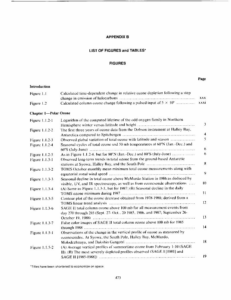
APPENDIX B
LIST OF FIGURES and TABLES*
FIGURES
Introduction
Figure 1. !
Figure 1.2
Chapter I--Polar
Figure 1.1.2-1
Figure 1.1.2-2
Figure 1.1.2-3
Figure 1.1.2-4
Figure I. 1.2-5
Figure I. 1.3- I
Figure I. 1.3-2
Figure 1.1.3-3
Figure 1. 1.3-4
Figure 1.1.3-5
Figure 1.1.3-6
Figure I. 1.3-7
Figure 1.1.5-I
Figure I.t.5-2
Calculated time-dependent change in relative ozone depletion following a step
change in emission of halocarbons ..................................................
Calculated column ozone change following a pulsed input of 5 x 10" ............
Ozone
Logarithm of the computed lifetime of the odd oxygen family in Northern
Hemisphere winter versus latitude and height ......................................
The first three years of ozone data from the Dobson instrument at Halley Bay,
Antarctica compared to Spitzbergen ................................................
Observed global variation of total ozone with latitude and season ................
Seasonal cycles of total ozone and 50 mb temperatures at 60°N (Jam-Dec.) and
60°S (July-June) ......................................................................
As in Figure 1.1.2-4, but for 80°N (Jan.-Dec.) and 80°S (July-June) ...............
Observed long-term trends in total ozone from the ground-based Antarctic
stations at Syowa, Halley Bay, and the South Pole ................................
TOMS October monthly mean minimum total ozone measurements along with
equatorial zonal wind speed .........................................................Seasonal decline in total ozone above McMurdo Station in 1986 as deduced by
visible, UV, and IR spectroscopy, as well as from ozonesonde observations ....
(A) Same as Figure 1.1.3-3, but tbr 1987; (B) Seasonal decline in the daily
TOMS ozone minimum during 1987 .................................................
Contour plot of the ozone decrease obtained from 1978-1988; derived from a
TOMS linear trend analysis .........................................................
SAGE !I total column ozone above 100 mb ['or all measurement events from
day 270 through 293 (Sept. 27- Oct., 20 1985, 1986, and 1987; September 26-
October 19, 1988) ....................................................................
False color images of SAGE Ii total column ozot_e above 100 mb for 1985
through 1988 ..........................................................................
Observations of the change in the vertical profile of ozone as measured by
ozonesondes. At Syowa, the South Pole, Halley Bay, McMurdo,
Molodezhnaya, and Dakshin Gangotri ..............................................
(A) Average vertical profiles of summertime ozone from February I-10 (SAGE
1I). (B) The most severely depleted profiles observed (SAGE I [1981] and
SAGE 11 ll985-1988[) ................................................................
*Titles have been shortened to economize on space.
Page
xxx
xxxi
3
4
5
6
6
8
9
10
11
12
13
14
18
19
473
FIGURES
Figure I. 1.5-3
Figure I. 2. I- 1
Figure 1.2.2-1
Figure 1.2.2-2
Figure 1.2.2-3
Figure 1.2.2-4
Figure 1.2.2-5
Figure 1.2.2-6
Figure 1.2.2-7
Figure 1.2.2-8
Figure 1.2.3-1
Figure 1.2.3-2
Figure 1.2.3-3
Figure 1.2.4-1
Figure 1.3.2-1
Figure 1.3.2-2
Figure 1.5.1-1
Figure 1.5.1-2
Figure .5.2- I
Figure .5.2-2
Figure .5.2-3
Figure .6.1-1
Figure .6.1-2
Figure .6.1-3
Figure .6.1-4
Figure .6. I-5
Figure .6. !-6
Figure .6.1-7
Trend in total ozone at 18 km observed from ozonesondes at McMurdo Station
in 1986 and 1987 ......................................................................
(Left) Vertical profiles of cloud particles observed during balloon soundings at
McMurdo Station in September, 1988. (Right) Particle size distributions at
various altitudes ......................................................................
Observations of PSC sightings (per week) from SAM II during 1979, 1980, 1981,
1982, and 1984 for May through October in the Southern Hemisphere vortex ...
As inFigure 1.2.2-1, but for 20, 22, and 24 km ......................................
As in Figure 1.2.2-1, but for 1985 through 1988 ....................................
As in Figure !.2.2-3, but for 20, 22, and 24 km .....................................
As in Figure 1.2.2-1, but for November through April in the Northern
Hemisphere vortex for the 1978-1979 through 1983-1984 winter seasons .........
As in Figure 1.2.2-5, but for 20, 22, and 24 km .....................................
As in Figure 1.2.2-5, but for 1984-1985 through 1988-1989 .........................
As in Figure 1.2.2-7, but for 20, 22, and 24 km .....................................
SAM II optical depth integrated from 2 km above the tropopause to 30 km, for
the Northern and Southern Hemispheres ...........................................
Observations of SAM 11 PSC sightings for Antarctica from 1979 through 1988 at
14, 16, and 18 kin, during the month of October ...................................
As in Figure 1.2.3-2, but for September ............................................
Changes in net heating caused by mountain PSCs with and without cirrus .......
Plot of the flight track data for the encounter with a PSC event on August 17,
1987 ...................................................................................
Observations of the percent of total observed nitrate in the particulate phase as
a function of time for September 4, 1987 ...........................................
CIO dimer thermal decomposition and photolysis rates ...........................
Calculated time behavior of CIO and CIONO2 during Arctic spring for three
different cases ........................................................................
Absorption cross sections of CIOOCI ...............................................
Rate constants for the CIO + CIO + M _ CI,O__ + M reaction, with N2
as the third body M ..................................................................
Photolysis rates for CI_,O> HOCI, CI> HNO_, and 02 at 70°S at noon as a
function of day, at the 50 mb level ..................................................
Observed CIO mixing ratio latitude gradients on the 425 and 450 K potential
temperature surfaces averaged over the AAOE mission period ...................
The vertical profile of CIO mixing ratio within the southern polar vortex, from
ground-based microwave measurements and in situ measurements ...............Diurnal variation of the column abundance of CIO below about 25 km at
McMurdo Station, Antarctica .......................................................
Diurnal variation of the column abundance of OCIO above McMurdo Station
September 18-19, 1986 ...............................................................
Daily measurements of the sunset OCIO column abundances above McMurdo
Station in 1986 and 1987 .............................................................
Observed distribution of the CIONO: column abundance, a function of latitude
relative to the edge of the vortex in August and September, 1987 .................
Observed latitude gradients of HCi and HF on the 24th of September and
2nd of October, 1987 .................................................................
Page
20
25
28
29
29
30
31
31
32
32
33
34
35
38
41
42
47
5O
51
52
53
56
56
57
58
59
60
61
474
Figure
Figure
Figure
Figure
Figure
Figure
Figure
Figure
Figure
Figure
Figure
Figure
Figure
Figure
Figure
Figure
Figure
Figure
Figure
Figure
Figure
Figure
Figure
Figure
Figure
Figure
Figure
1.6.2-1
1.6.2-2
1.6.2-3
1.6.2-4
1.6.2-5
1.6.2-6
1.6.2-7
1.6.2-8
1.6.3-1
1.6.3-2
1.6.3-3
1.6.3-4
!.6.3-5
1.6.4-1
1.6.4-2
1.6.4-3
1.6.4-4
1.6.4-5
1.7.1-I
1.7.1-2
1.7.1-3
1.7.1-4
1.7.1-4
1.7.1-4
1.7.1-5
1.7.1-6
1.7.1-7
FIGURES
Page
Observations of the latitude gradient of column NO_ in the Southern
Hemisphere ........................................................................... 63
Observations of the seasonal trend in morning and evening twilight slant
column NO2 abundances from three Antarctic sites ............................... 64
Total NO2 (a), total O, (b), and 50 mb temperature (c) at Molodezhnaya in 1987
and Mirny in 1988 .................................................................... 65
Cross section of NO2 vs. latitude and pressure for the period September 27 to
October 7, 1987, from SAGE 1I observations ...................................... 66
Observed column of HNO3 plotted as a function of latitude relative to the edge
of the polar vortex in August and September, 1987 ................................ 66
Measurements of total reactive nitrogen (NO_) versus N20 obtained from
aircraft observations ................................................................. 67
Observed total reactive nitrogen profile as a function of potential temperature .. 69
Observed NO mixing ratios versus latitude relative to the chemically
perturbed region ...................................................................... 70
Observed latitude gradient of H30 on September 22, 1987 near 450 K surface ... 70
Cross section of H20 vs. latitude and pressure for the period September 27 to
October 7, 1987, measured by SAGE II ............................................ 71
BrO mixing ratios versus latitude for nine flights from about 54 ° and 72°S, taken
between August 28 and September 22, 1987 ........................................ 72
Variation of the BrO mixing ratio with potential temperature ..................... 73
Diurnal variation of the BrO slant column at McMurdo Station ................... 74
Calculated and observed CIO mixing ratios on the 428 K surface, 4-12
September, 1987 ...................................................................... 76
Calculated and observed CIO mixing ratio profiles at 72°S, 4th/9th September,
1987 ................................................................................... 77
Observed NO and CIO mixing ratios from an aircraft flight on August 28, 1987 78
Observed and calculated rates of ozone decline for different CIO dimer
formation rates as a function of potential temperature ............................. 79
Observed October mean total ozone abundance over Halley Bay, Antarctica ... 81
The range, near 90 mb, of minimum brightness temperatures poleward of
latitude 20, computed daily for winter and spring from 1980 to 1988 .............. 83
Comparison of N20 vertical profiles during austral winter-spring, austral
summer, and austral winter .......................................................... 84
Vertical distributions of the total amount of chlorine bonded in the five most
abundant anthropogenic halocarbons ............................................... 85
(i) Monthly mean perspectives during June 1982 of the three-dimensional
structure of the westerly vortex in the Southern Hemisphere ..................... 86
(ii) As for Figure 1.7. I(i), but for September ....................................... 87
(iii) As for Figure i.7. I(i), but for October ......................................... 87
Time of the reversal of the zonal wind at latitude 60 ° , and of the temperature
difference between 60 ° and 85 ° for the Northern and Southern Hemispheres .... 88
Evolution of zonal-mean total ozone (Dobson units) derived from the TOMS
instruments, 1987 and 1988 .......................................................... 90
Minimum brightness temperature near 90 mb (Channel 24 of the MSU) in the
Southern Hemisphere during 1987 .................................................. 91
475
FIGURES
Figure 1.7. I-8
Figure 1.7.1-9
Figure 1.7.1-10
Figure 1.7. l- I I
Figure 1.7.1-12
Figure 1.7.1-13
Figure 1.7.1-14
Figure 1.7.1-15
Figure 1.7.1-16
Figure 1.7.1-17
Figure 1.7.1-18
Figure 1.7.1-19
Figure 1.7.1-20
Figure 1.7. I-2 I
Figure 1.7.1-22
Figure 1.7.1-23
Figure 1.7.2-1
Figure 1.7.2-2
Figure 1.7.2-2
Figure 1.7.2-3
Figure 1.7.4-1
Figure 1.7.4-2
Figure 1.7.4-3
Figure 1.7.4-4
Figure 1.7.4-5
Figure 1.7.4-6
Figure 1.7.4-7
Figure 1.8.1-1
Figure 1.8.2-1
Figure 1.8.2-2
Figure 1.8.2-3
Figure i.8.2-4
Page
The fractional area of the Southern Hemisphere over which minimum
temperatures near 90 mb in 1987 fell below t93 K ................................. 91
As for Figure 1.7.1-7 but for 1988 ................................................... 92
As for Figure 1.7.1-8 but for 1988 ................................................... 92
lsentropic maps of Ertel's potential vorticity and winds on the 500 K isentropic
surface in the Southern Hemisphere on 1 August 1987 ............................ 93
As for Figure 1.7. I-I 1, but for 31 October 1987 .................................... 94
As for Figure 1.7. I-1 I, but on I August 1988 ....................................... 94
As for Figure 1.7. I-1 I, but on 20 October 1988 .................................... 95
As for Figure 1.7. I-1 I, but for the Northern Hemisphere on 18 January 1989 .... 96
As for Figure 1.7. l-l I, but for the Northern Hemisphere on 20 February 1989 .. 97
Minimum brightness temperature derived from channel 24 of the MSU in the
Northern Hemisphere for December through May ................................. 98
The total ozone fields (in Dobson units) from November 1978 to October 1987
with annual cycle removed .......................................................... 99
As for Figure 1.7.1-18, but after application of a broad-band filter ................ 100
Variation in October mean total ozone and 70 mb temperature over the
South Pole ............................................................................ 101
As for Figure 1.7.1-20, but for the April mean in the Northern Hemisphere ..... 101
Correlation of August-September winds over Singapore at 30 mb with the total
ozone decline rate in September .................................................... 102
Ozone mixing ratio variation at the maximum of the I l-year solar cycle ......... 103
An example of a mini-hole over the Antarctic Peninsula on 5 September 1987 ... 105
(i) Longitude/pressure cross sections on 5 September 1987 at latitude 65°S from
90°W to 30°W, and from 250 to 30 mb ............................................... 106
(ii) As for Figure 1.7.2-2 (i) .......................................................... 107
A sequence of potential vorticity distributions on the 428 K surface of potential
temperature ........................................................................... 108
Ertel's potential vorticity on the 600 K isentropic surface ......................... I i !
TOMS total ozone. Monthly variation of difference between 1987-1988 average
and 1979-1980 average as a function of latitude .................................... 112
Percent change in the simulated steady-state seasonal and latitudinal
distribution of zonal-mean column Ozone ........................................... 113
Percent difference in zonal-mean column ozone for Antarctic ozone hole ....... 114
Percent difference in the integrated global and hemispheric column ozone for
Antarctic ozone hole ................................................................. 116
TOMS total ozone for the Southern Hemisphere .................................. 117
Difference between Ertel's potential vorticity (500 K isentropic surface) for8 December and 14 December 1987 ................................................. 118
Linear trends calculated from NMC data for the period 1979-1986, for August,
September, November, and December ............................................. 119
Deviations of temperatures 1958-1988 (°C) for Angell's (1988b) six south polar
stations ............................................................................... 120
Monthly mean temperatures at 100 mbar for Halley Bay, 1958-1988 .............. 121
Temperatures at 100 mbar as a function of month from Halley Bay .............. 122
Deviation of NMC zonal mean temperatures for 1987 from the 1979-1986 mean
for September to December ......................................................... 123
476
FIGURES
Figure 1.8.3-1
Figure 1.8.3-2
Figure 1.9-1
Figure 1.9-2
Figure 1.9-3
Figure 1.9-4
Figure 1. I0.1- I
Figure 1.10.1-2
Figure !. 10.1-3
Figure I. 10. I-4
Figure 1.10.1-5
Figure I. 10. I-6
Figure I. 10. I-7
Figure 1.10.2-1
Figure 1.10.2-2
Figure 1.10.2-3
Page
1252-D model temperatures at 39 mb and 76°S with and without an imposed ozone
hole ...................................................................................
Deviation of zonal mean temperature for a calculation with an imposed ozone
hole from a control run without the hole, using the NCAR Community Climate
Model ................................................................................. 126
Ratio of biologically effcctive downward radiation computed for a range ofozone values at McMurdo ........................................................... 127
Computed time history of erythemal irradiance for local noon and clear skiesover Palmer Station .................................................................. 129
Spectra of UV solar irradiance measured from Palmer Station at local noon ..... 130Ratio of noontime irradiance for 295-305 nm to that for 335-345 nm, for the
period 19 September and 21 December 1988 ....................................... 131
Observation of the Noxon cliff ...................................................... 131
The mean annual cycle ofNO_ at 71°N (Point Barrow, Alaska) ................... 132
Variation of total NO2 column abundance over Point Barrow, Alaska (7 I°N) in
three different winter-spring seasons ............................................... 133
NOx (NO + NO:) mixing ratio profiles observed on balloon flights using a
chemiluminescent detector .......................................................... 134
Zonally and monthly averaged HNO_ mixing ratio distributions for November,
December, and January from LIMS observations ................................. 136
Latitude gradients of HC1 and HF in the Northern Hemisphere .................. 137
Observations of the nighttime abundance of OCIO versus lunar zenith angle at
various locations ..................................................................... 138
Ozone partial pressure and mixing ratio profiles measured at Kiruna, Sweden,
on 23 January, 1989 .................................................................. 140
NMC temperatures at 30 mb for the 1988-1989 Northern Hemisphere winter-
spring season ......................................................................... 141
NMC temperatures at 30 mb tbr the 1975-1976 Northern Hemisphere winter-142spring season .........................................................................
Chapter 2--Global Trends
Figure 2.1-! Time-lines of measurements available for use in ozone trend analyses at the164present time ..........................................................................
Figure 2.1-2 Location of Dobson and M-83 stations ............................................. 166
Figure 2.1-3 Time-lines for ozone-measuring systems that are projected to be operating over175the next decade ......................................................................
Figure 2. l-4a Comparison between archived TOMS total ozone data and Dobson data ........ 182
Figure 2. I-4b Comparison between TOMS total ozone data where diffuser plate degradation
was corrected by the "pair justification" method and Dobson data ............... 183
Figure 2. I-5 Samples of profile pairs measured by ozonesondes and the SAGE I instrument
and the mean percentage difference between the ozonesondes and the SAGE 1186ozone .................................................................................
Figure 2.1-6 Samples of profile pairs measured by ozonesondes and the SAGE 1I instrument
and the mean percentage difference between the ozonesondes and the SAGE II187
ozone .................................................................................
Figure 2.1-7 Mean differences between SAGE I and ozonesondes and SAGE !1 andozonesondes .......................................................................... 188
477
FIGURES
Figure 2.2- I
Figure 2.2-2a
Figure 2.2-2b
Figure 2.2-2c
Figure 2.2-3
Figure 2.2-4
Figure 2.2-5
Figure 2.2-6
Figure 2.2-7
Figure 2.2-8
Figure 2.2-9a
Figure 2.2-9b
Figure 2.2-10
Figure 2.2-11
Figure 2.2-12
Figure 2.2-13
Figure 2.3-1
Figure 2.3-2
Figure 2.3-3
Figure 2.3-4
Figure 2.3-5
Figure 2.3-6
Figure 2.3-7
Figure 2.3-8
Figure 2.4-1a
Figure 2.4-1b
Figure 2.4-Ic
Figure 2.4- Id
Page
Monthly and zonally averaged Dobson total ozone values versus time alter
removal of seasonal, QBO, solar cycle, and nuclear test effects .................. 197
Regional plots of Dobson total ozone after removal of seasonal, solar, QBO,
and nuclear test effects for North America, Europe, and Japan ................... 198
Same as 2.2-2a for winter months (December-March) ............................. 199
Same as 2.2-2a for summer months (May-August) ................................. 200
Plots of Dobson total ozone monthly averages combined into time series for
each latitudinal zone ................................................................. 201
Individual trend estimates for the period 1970-1986 using the AS2 model ........ 203
Same as Figure 2.2-4 except trends are fitted only through October 1982 ........ 205
Same as Figure 2.2-4 except trends are fitted using updated data into 1988 ...... 208
Differences between estimated trends into 1988 versus trends through 1986 ..... 210
Solar coefficient computed for 25 Northern Hemisphere stations from the
AS2 model ............................................................................ 211
Geographic structure in total ozone changes based on TOMS .................... 212
Same as Figure 2.2-9a for Southern Hemisphere ................................... 213
Geographic pattern of change in total ozone derived from SBUV for the
Northern Hemisphere winter and summer ......................................... 215
Geographic pattern of change in total ozone derived from SBUV for the
Southern Hemisphere winter and summer .......................................... 215
Changes in total ozone based on eight-year data sets from the SBUV and
TOMS instruments ................................................................... 217
Changes in total ozone derived from Dobson data for the eight-year period over
which SBUV measurements are available .......................................... 218
Latitudes of the SAGE I and SAGE I1 sampling locations for sunset ............. 222
Zonal mean ozone number density at 30 km for SAGE 1 during the period 2/79-
! 1/81 and SAGE I1 during the period 10/84-I 1/87 for five latitude bands .......... 223
Daily mean ozone number density at 35 km for SAGE 11 for twelve latitude
bands ................................................................................. 224
Mean percentage difference between SAGE 11 and SAGE 1 versus altitude
computed from the intersection of SAGE 1 with SAGE II ......................... 225
Deseasonalized Umkehr data at Arosa for layers 4-9, unadjusted for aerosols,
for the period January 1977 through December 1987 ............................... 227
Stratospheric aerosol optical thickness derived from lidar data for the period
1977-1987 ............................................................................. 228
Umkehr data trend estimates from 10 individual Umkehr stations for layers 4-9,
for the period January 1977 through December 1987 ............................... 229
Trend estimates derived from ozonesondes measurements at 9 stations for 15
fractional Umkehr layers ............................................................ 233
Seasonal temperatures with the long-term seasonal averages removed and
smoothed 1-2-1 in time for Angell, Berlin, NMC, MSU, SSU ..................... 238
Seasonal temperatures with the long-term seasonal averages removed and
smoothed 1-2-1 in time: NMC; SSU Channels 25 and 26 × ....................... 239
Seasonal temperatures with the long-term seasonal averages removed and
smoothed I-2-1 in time: NMC; SSU Channel 26 ................................... 240
Seasonal temperatures with the long-term seasonal averages removed and
smoothed 1-2-1 in time: NMC 5-1 mb; SSU Channels 27 and 36 X ............... 241
478
FIGURES
Figure 2.4-2
Figure 2.4-3
Figure 2.4-4
Figure 2.4-5
Figure 2.4-6
Figure 2.5-1
Figure 2.5-2
Figure 2.5-3
Figure 2.5-4
Figure 2.5-5
Figure 2.5-6
Figure 2.5-7
Figure 2.5-8
Figure 2.5-9
Figure 2.5-10
Figure 2.6- I
Figure 2.7-1
Figure 2.7-2
Page
Lidar temperature and SSU channel 27 brightness temperature from 1981to 1987 ................................................................................ 242
Lidar and NMC temperature at 42 km .............................................. 242
Comparison of the 10.7 cm solar flux, in 10-:-"W/(m: Hz), and the 30-rob
temperature, in °C, at the North Pole ............................................... 243
Summary of global stratospheric temperature differences (1985 and 1986 minus
the average of 1979 and 1980) ....................................................... 244
As in Figure 2.4-4, except for Tropics and including rocket stations .............. 245
Halocarbon (pptv) and nitrous oxide (ppbv) observations at Cape Grim,
Tasmania, as part of the GAGE program ........................................... 248
CHCIF: (pptv) observations at Cape Grim. Tasmania, from the Oregon
Graduate Center flask sampling program ........................................... 249
CH,CI (pptv) observations at Cape Grim, Tasmania, from the Oregon Graduate
Center flask sampling program ...................................................... 249
CHCL (pptv) observations at Cape Grim, Tasmania, from the Oregon Graduate
Center flask sampling program ...................................................... 250
Long-term trends of N,O from the GMCC program, the SIO program, the
OGC-ALE program, the FIAER-CSlR program, and CSIRO-GAGE data ....... 252
Long-term trends of CH4 from the CSIRO global program and the FIAER-CSIR
program at Cape Point, South Africa ............................................... 254
The global distribution, seasonality, and trend of CH4 from the GMCCnetwork ............................................................................... 255
Long-term trends of CO from the CSIRO network and from Cape Point, SouthAfrica ................................................................................. 257
The temporal behavior of the CO, trends observed at the GMCC stations ....... 258
Surface ozone measurements at the GMCC stations, at Cape Point, South
Africa, and at Cape Grim, Tasmania ................................................ 260
Aerosol integrated backscatter coefficient over the period 1974-88 ............... 262
Solar spectral irradiance incident on the Earth's surface computer for January
and July at latitudes 34.5 °, 46.0 °, and 58.5°N ....................................... 264
Percent changes in solar spectral irradiance between 1970 and 1986 computed
tbr January, March, and July at latitudes 34.5 °, 46.0 °, and 58.5°N ................ 266
Chapter 3--Theoretical Predictions
Figure 3.1-1 Schematic diagram showing an algorithm for determining the coupled set of
transport parameters with prescribed T as input ................................... 287
Figure 3. i-2 Total ozone field on 28 February 1989 as measured by TOMS and as modeled
from a January I initial condition ................................................... 291
Figure 3. I-3 Two-dimensional distribution of tropospheric source gas X from nine models forthe month of December .............................................................. 295
Figure 3.1-4 Two-dimensional distribution of the CIO/HCI ratio from nine models ............ 298
Figure 3. I-5 Zonally and monthly averaged distribution of nitrous oxide observed in January
1979 by SAMS and calculated by GSFC model .................................... 301
Figure 3.1-6 Same as in Figure 3.1-5 but for methane ............................................ 302
Figure 3.1-7 Zonally and monthly averaged distribution of nighttime NO: observed in
January 1979 by LLMS .............................................................. 303
479
FIGURES
Figure 3.1-8
Figure 3.1-9
Figure 3.1-10
Figure 3. I- I I
Figure 3.2- I
Figure 3.2-2
Figure 3.2-3
Figure 3.2-4
Figure 3.2-5
Figure 3.2-6
Figure 3.2-7
Figure 3.2-8
Figure 3.2-9
Figure 3.2-10
Figure 3.2-1 !
Figure 3.2-12
Figure 3.2-13
Figure 3.2-14
Figure 3.2-15
Figure 3.2-16
Figure 3.2-17
Figure 3.2-18
Figure 3.2-19
Figure 3.2-20
Page
Same as in Figure 3. I-7 but for nitric acid .......................................... 304
Zonally and monthly averaged distribution of ozone for January based on data
obtained by SBUV and distribution by different two-dimensional models ....... 307
Latitudinal and seasonal variation of the ozone column abundance based on
satellite observations (TOMS) and different model calculations .................. 312
Comparison between one-dimensional mixing ratio profiles of chemically active
trace gases measured by ATMOS ................................................... 316
Time history, 1960-2060, of mean tropospheric concentrations of the trace gases
assumed for the different scenarios ................................................. 319
Time history, 1980-2060, of total atmospheric chlorine and total atmospheric
bromine from the different scenarios ............................................... 321
Dobson map of percent change in column ozone from 1960 to 1980 using the
specified trace-gas scenario .......................................................... 329
Latitude-by-altitude contour map of the percent change in local ozone
concentration from 1960 to 1980 for the specified trace-gas scenario ............. 333
Time-line of the percent change in column ozone as a function of latitude for
the months of March from 1980 through 2060 for scenario A! .................... 338
Dobson map of percent change in column ozone from 1980 to 2020 using
scenario A I ........................................................................... 340
Dobson map of percent change in column ozone from 1980 to 2060 usingscenario A 1 ........................................................................... 342
Latitude-by-altitude contour map of the percent change in local ozone
concentration from 1980 to 2060 for scenario A I ................................... 347
Time-line vs. latitude of the percent change in column ozone during March from
1980 to 2060 for scenario A2 ......................................................... 351
Dobson map of percent change in column ozone from 1980 to 2060 using
scenario A2 ........................................................................... 352
Latitude-by-altitude map of the percent change in local ozone concentration
from 1980 to 2060 for scenario A2 ................................................... 353
Temperature change (K) for December (scenario A I: 1980-2060) from the AER
and WisCAR models ................................................................. 354
Zonal wind and zonal wind change from December 1980 to December 2060 for
the WisCAR model (scenario AI) ................................................... 355
Net radiative heating (K/day) for December 1980 in the AER and WisCAR
models ................................................................................ 356
Change in net radiative heating (K/day) from December 1980 to December 2060
(scenario AI) in the AER and WisCAR models .................................... 357
Time-line vs. latitude of the percent change in column ozone during March from
1980 to 2060 for scenario AI ......................................................... 359
Dobson map of percent change in column ozone from 1980 to 2060 using
scenario B I ........................................................................... 360
Latitude-by-altitude map of the percent change in local ozone concentration
from 1980 to 2060 for scenario BI ................................................... 361
Time-line vs. latitude of the percent change in column ozone during March from
1980 to 2060 for scenario CI ......................................................... 363
Dobson map of percent change in column ozone from 1980 to 2060 using
scenario C 1 ........................................................................... 364
480

Figure3.2-21
Figure3.2-22
Figure3.2-23
Figure3.2-24
Figure3.2-25
Figure3.2-26
Figure3.2-27
Figure3.2-28
Figure3.2-29
Figure3.2-30
Figure3.2-31
Figure3.2-32
Figure3.2-33
Figure3.2-34
Figure3.2-35
Figure3.2-36
Figure3.2-37
Figure3.2-38
Figure3.2-39
Figure3.2-40
Figure3.2-41Figure3.2-42Figure3.2-43Figure3.2-44
FIGURES
Page
Latitude-by-altitude map of the percent change in local ozone concentration
from 1980 to 2060 for scenario CI ................................................... 364
Time-line vs. latitude of the percent change in column ozone during March from
1980 to 2060 for scenario DI ......................................................... 365
Dobson map of percent change in column ozone from 1980 to 2060 using
scenario D1 ........................................................................... 366
Latitude-by-altitude map of the percent change in local ozone concentration
from 1980 to 2060 for scenario DI ................................................... 368
Time-line vs. latitude of the percent change in column ozone during March from
1980 to 2060 for scenario D2 ......................................................... 371
Dobson map of percent change in column ozone from 1980 to 2060 using
scenario D2 ........................................................................... 371
Latitude-by-altitude map of the percent change in local ozone concentration
from 1980 to 2060 for scenario D2 ................................................... 372
Time-line vs. latitude of the percent change in column ozone during March from
1980 to 2060 for scenario D3 ......................................................... 372
Dobson map of percent change in column ozone from 1980 to 2060 using
scenario D3 ........................................................................... 373
Latitude-by-altitude map of the percent change in local ozone concentration
from 1980 to 2060 for scenario D3 ................................................... 373
Time-line vs. latitude of the percent change in column ozone during March from
1980 to 2060 for scenario D4 ......................................................... 374
Dobson map of percent change in column ozone from 1980 to 2060 using
scenario D4 ........................................................................... 375
Latitude-by-altitude map of the percent change in local ozone concentration
from 1980 to 2060 for scenario D4 ................................................... 375
Two-year sequence of percent change in column ozone from the Cambridge
model with PSC chemistry in the Northern Hemisphere .......................... 376
Dobson maps of percent change in column ozone from 1960 to 2060 from the
WisCAR model with and without heterogeneous chemistry on PSCs for
scenario A 1 ........................................................................... 377
Dobson maps of percent change in column ozone from 1960 to 1985 and from
1985 to 2060 from the AER model using scenario BI .............................. 378
Dobson maps of percent change in column ozone from 1985 to 2050 from the
Oslo model with and without heterogeneous chemistry on the natural sulfate380
layer ..................................................................................
Dobson maps of percent change in column ozone from 1985 to 2060 from the
AER model using scenario B1 ....................................................... 381
Action spectra used as weighting functions to calculate biologically effective381radiation ..............................................................................
Daily doses for 1979/80 based on ozone column from TOMS measurements386normalized to Dobson ...............................................................
Daily dose changes from 1960 to 1980, GSFC2 model ............................. 388
Daily dose changes from 1960 to 2060, GSFC2 model, scenario AI .............. 389
Daily dose changes from 1960 to 2060, GSFC2 model, scenario DI .............. 390
Daily DNA damage dose changes from 1980 to 2060, WisCAR model, scenarios391A l, A2, and D I .......................................................................
481
FIGURES
Figure 3.2-45
Figure 3.2-46
Page
Figure 4.2-1
Figure 4.2-2
Figure 4.3- I
Figure 4.3-2
Figure 4.3-3
Figure 4.3-4a
Figure 4.3-4b
Figure 4.3-4c
Figure 4.3-4d
Figure 4.3-4e
Figure 4.3-5a
Figure 4.3-5b
Figure 4.3-5c
Figure 4.3-5d
Figure 4.3-5e
Figure 4.3-6
Figure 4.3-7
Figure 4.3-8a
Figure 4.3-8b
Figure 4.3-9a
Transformed Eulerian mean vertical velocity for a 240-day average simulation
performed with the NCAR Community Climate Model ............................ 394
As in Figure 3.3-40 but for the ozone reduction scenario shown in Figure
3.3.41b; percentage change in ozone from the two-dimensional model of Ko
et al., 1985 ............................................................................ 394
Chapter 4---Halocarbon Ozone Depletion Potentials and Global Warming Potentials
Reactions governing concentrations of OH and HO__ .............................. 411
Schematic presentation of the measured vertical distribution of NO and NO_
over midlatitude oceanic and coastal regions ....................................... 419
Calculated column ozone change in the DuPont 1-D model following a pulsed
input of 5.0 x 10'_kgofspecified gas ............................................... 425
Atmospheric concentrations of halocarbons with 5- and 100-year lifetimes
following onset of a constant emission of each compound ......................... 426
Calculated latitudinal and seasonal steady-state ozone change from emission of
CFC-I ! necessary for global I% change in total ozone (LLNL 2-D model) ...... 435
Calculated latitudinal and seasonal steady-state ozone change from emission of
CFC-12 necessary to give I% change in total ozone (LLNL 2-D model) ......... 436
Calculated latitudinal and seasonal relative ozone depletion of CFC-12 (LLNL
2-D model) ............................................................................ 437
Calculated latitudinal and seasonal relative ozone depletion of CFC-12 (AER
2-D model) ............................................................................ 437
Calculated latitudinal and seasonal relative ozone depletion of CFC-12 (Oslo
2-D model) ............................................................................ 438
Calculated latitudinal and seasonal relative ozone depletion of CFC-12 (DuPont
2-D model) ............................................................................ 438
Calculated latitudinal and seasonal steady-state ozone change necessary to give
I% change in total ozone from emission of HCFC-22 (LLNL 2-D model) ....... 439
Calculated latitudinal and seasonal relative ozone depiction of CFC-22 (LLNL
2-D model) ............................................................................ 439
Calculated latitudinal and seasonal relative ozone depletion from emission ofHCFC-22 (AER 2-D model) ......................................................... 440
Calculated latitudinal and seasonal relative ozone depletion from emission of
HCFC-22 (Oslo 2-D model) .......................................................... 440
Calculated latitudinal and seasonal relative ozone depletion from emission of
HCFC-22 (DuPont 2-D model) ...................................................... 441
Calculated CFC-I l profiles from transport sensitivity study at 75°S at equinox
(AER 2-D model) ..................................................................... 443
Calculated CFC-11 profiles from transport sensitivity study at Equator at
equinox (AER 2-D model) ........................................................... 443
Calculated HCFC-22 profiles from transport sensitivity study at 75°S at equinox
(AER 2-D model) ..................................................................... 444
Calculated HCFC-22 profiles from transport sensitivity study at Equator at
equinox (AER 2-D model) ........................................................... 444
Calculated total ozone abundance (Dobson units) from transport sensitivity
studies (case I and case 2 ............................................................ 445
482
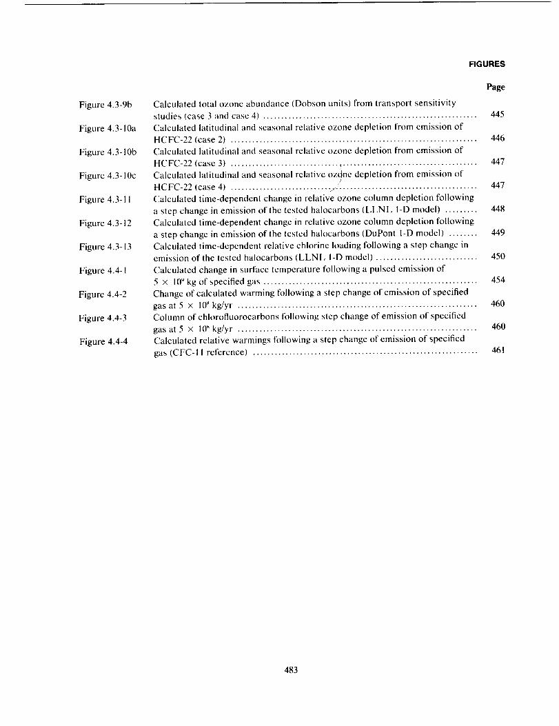
Figure4.3-9b
Figure4.3-10a
Figure4.3-10b
Figure4.3-10c
Figure4.3-11
Figure4.3-12
Figure4.3-13
Figure4.4-I
Figure4.4-2
Figure4.4-3
Figure4.4-4
FIGURES
Page
Calculated total ozone abundance (Dobson units) from transport sensitivity
studies (case 3 and case 4) ........................................................... 445
Calculated latitudinal and seasonal relative ozone depletion from emission of
HCFC-22 (case 2) .................................................................... 446
Calculated latitudinal and seasonal relative ozone depletion from emission of
HCFC-22 (case 3) .................................................................... 447
Calculated latitudinal and seasonal relative oztlne depletion from emission of
HCFC-22 (case 4) ............................ ,_(. ..................................... 447
Calculated time-dependent change in relative ozone column depletion following
a step change in emission of the tested halocarbons (LLNL 1-D model) ......... 448
Calculated time-dependent change in relative ozone column depletion following
a step change in emission of the tested halocarbons (DuPont 1-D model) ........ 449
Calculated time-dependent relative chlorine loading following a step change in
emission of the tested halocarbons (LLNL I-D model) ............................ 450
Calculated change in surface temperature following a pulsed emission of
5 × 10⁹ kg of specified gas ........................................................... 454
Change of calculated warming following a step change of emission of specified
gas at 5 × 10_kg/yr .................................................................. 460Column of chlorofluorocarbons following step change of emission of specified
gas at 5 × I0 _ kg/yr .................................................................. 460
Calculated relative warmings following a step change of emission of specified
gas (CFC-i I reference) .............................................................. 461
483
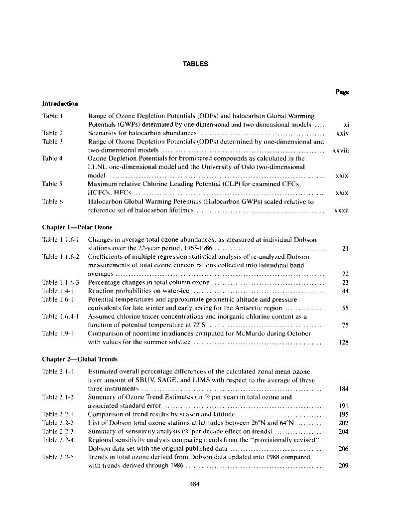
TABLES
Introduction
Table 1
Table 2
Table 3
Table 4
Table 5
Table 6
Page
Range of Ozone Depletion Potentials (ODPs) and halocarbon Global Warming
Potentials (GWPs) determined by one-dimensional and two-dimensional models .... xi
Scenarios for halocarbon abundances ................................................ xxiv
Range of ()zone Depletion Potentials (ODPs} determined by one-dimensional and
two-dimensional models .............................................................. xxviii
Ozone Depletion Potentials for brominated compounds as calculated in the
LLNL one-dimensional model and the University of Oslo two-dimensional
model .................................................................................. xxix
Maximum relative Chlorine Loading Potential (CLP) for examined CFCs,
HCFCs, HFCs ......................................................................... xxix
Halocarbon Global Warming Potentials (Halocarbon GWPs) scaled relative toreference set of halocarbon lifetimes ................................................. xxxii
Chapter I--Polar Ozone
Table I. 1.6-1 Changes in average total ozone abundances, as measured at individual Dobson
stations over the 22-year period, 1965-1986 .......................................... 21
Table I. 1.6-2 Coefficients of multiple regression statistical analysis of re-analyzed Dobsonmeasurements of total ozone concentrations collected into latitudinal band
averages ................................................................................ 22
Table 1.1.6-3 Percentage changes in total column ozone ........................................... 23
Table 1.4-1 Reaction probabilities on water-ice .................................................. 44
Table 1.6-1 Potential temperatures and approximate geometric altitude and pressure
equivalents for late winter and early spring for the Antarctic region ............... 55
Table 1.6.4-1 Assumed chlorine tracer concentrations and inorganic chlorine content as a
function of potential temperature at 72°S ............................................ 75
Table 1.9-I Comparison of noontime irradiances computed for McMurdo during Octoberwith values for the summer solstice .................................................. 128
Chapter 2--Global Trends
Table 2.1-1 Estimated overall percentage differences of the calculated zonal mean ozone
layer amount of SBUV, SAGE, and LIMS with respect to the average of these
three instruments ...................................................................... 184
Table 2. I-2 Summary of Ozone Trend Estimates (in % per year) in total ozone and
associated standard error ............................................................. 191
Table 2.2-1 Comparison of trend results by season and latitude ................................. 195Table 2.2-2 List of Dobson total ozone stations at latitudes between 26°N and 64°N .......... 202
Table 2.2-3 Summary of sensitivity analysis (% per decade effect on trends) ................... 204
Table 2.2-4 Regional sensitivity analysis comparing trends from the "provisionally revised"
Dobson data set with the original published data .................................... 206
Table 2.2-5 Trends in total ozone derived from Dobson data updated into t988 compared
with trends derived through 1986 ..................................................... 209
484
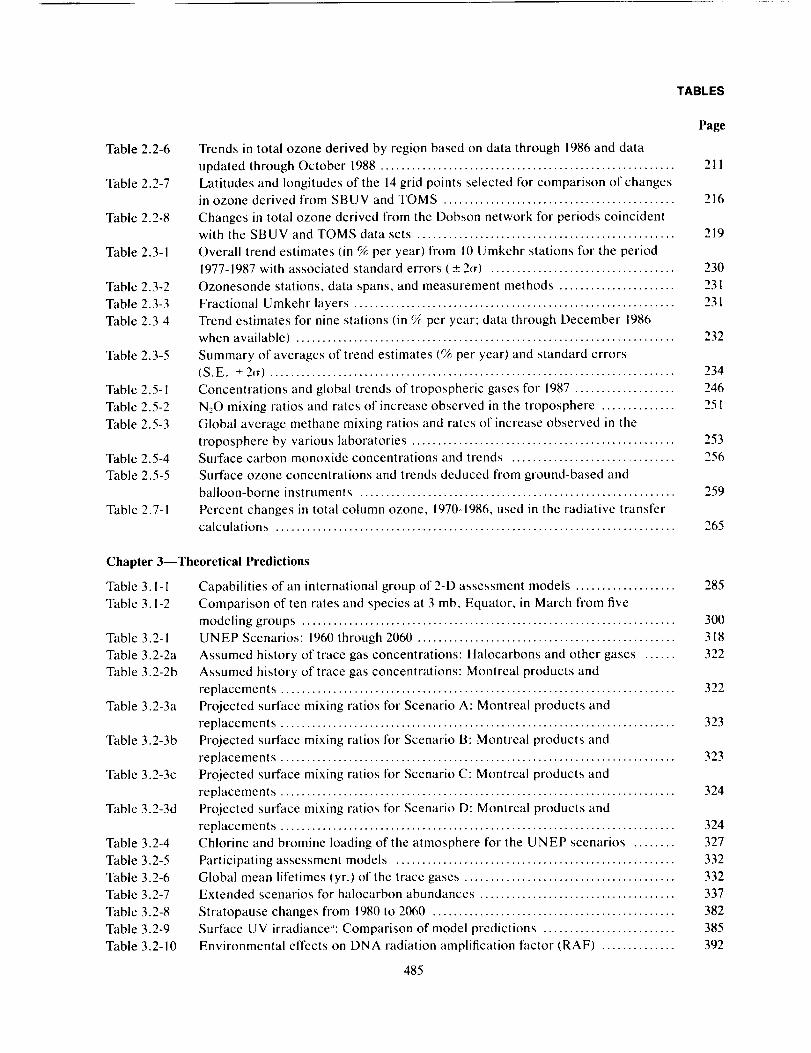
Table2.2-6
Table2.2-7
Table2.2-8
Table2.3-1
Table2.3-2Table2.3-3Table2.3-4
Table 2.3-5
Table 2.5-1
Table 2.5-2
Table 2.5-3
Table 2.5-4
Table 2.5-5
Table 2.7-1
TABLES
Page
Trends in total ozone derived by region based on data through 1986 and data
updated through October 1988 ........................................................ 211
Latitudes and longitudes of the 14 grid points selected for comparison of changes
in ozone derived from SBUV and TOMS ............................................ 216
Changes in total ozone derived from the Dobson network for periods coincident
with the SBUV and TOMS data sets ................................................. 219
Overall trend estimates (in % per year) from 10 Umkehr stations for the period
1977-1987 with associated standard errors (_ 2¢r) ................................... 230
Ozonesonde stations, data spans, and measurement methods ...................... 231
Fractional Umkehr layers ............................................................. 231
Trend estimates for nine stations (in % per year: data through December 1986
when available) ........................................................................ 232
Summary of averages of trend estimates (% per year) and standard errors
(S.E. _+2¢r) ............................................................................. 234
Concentrations and global trends of tropospheric gases for 1987 ................... 246
N20 mixing ratios and rates of increase observed in the troposphere .............. 251
Global average methane mixing ratios and rates of increase observed in the
troposphere by various laboratories .................................................. 253
Surface carbon monoxide concentrations and trends ............................... 256
Surface ozone concentrations and trends deduced from ground-based and
balloon-borne instruments ............................................................ 259
Percent changes in total column ozone, 1970-1986, used in the radiative transfer
calculations ............................................................................ 265
Chapter 3--Theoretical Predictions
Table 3. I- 1 Capabilities of an international group of 2-D assessment models ................... 285
Table 3. I-2 Comparison of ten rates and species at 3 mb, Equator, in March from five
modeling groups ....................................................................... 300
Table 3.2-1 UNEP Scenarios: 1960 through 2060 ................................................. 318
Table 3.2-2a Assumed history of trace gas concentrations: Halocarbons and other gases ...... 322
Table 3.2-2b Assumed history of trace gas concentrations: Montreal products and
replacements ........................................................................... 322
Table 3.2-3a Projected surface mixing ratios for Scenario A: Montreal products and
replacements ........................................................................... 323
Table 3.2-3b Projected surface mixing ratios for Scenario B: Montreal products and
replacements ........................................................................... 323
Table 3.2-3c Projected surface mixing ratios for Scenario C: Montreal products and
replacements ........................................................................... 324
Table 3.2-3d Projected surface mixing ratios for Scenario D: Montreal products and
replacements ........................................................................... 324
Table 3.2-4 Chlorine and bromine loading of the atmosphere for the UNEP scenarios ........ 327
Table 3.2-5 Participating assessment models ..................................................... 332
Table 3.2-6 Global mean lifetimes {yr.) of the trace gases ........................................ 332
Table 3.2-7 Extended scenarios for halocarbon abundances ..................................... 337
Table 3.2-8 Stratopause changes from 1980 to 2060 .............................................. 382
Table 3.2-9 Surface UV irradiance_': Comparison of model predictions ......................... 385
Table 3.2-10 Environmental effects on DNA radiation amplification factor (RAF) .............. 392
485
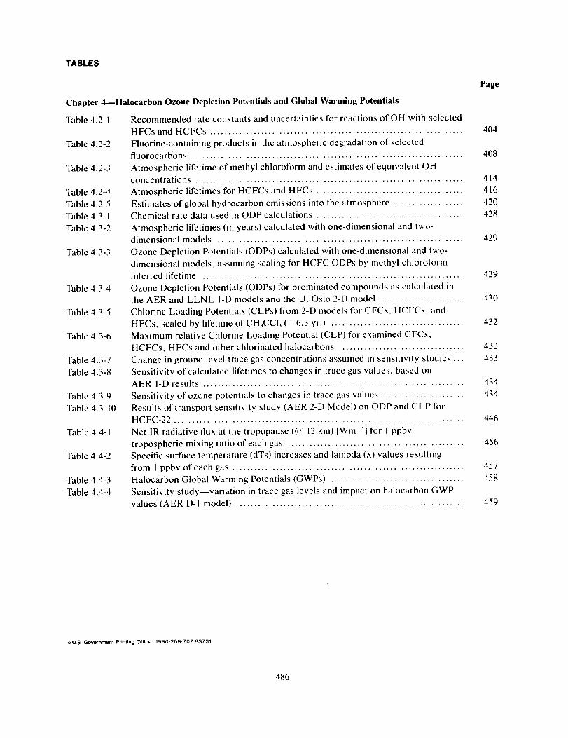
TABLES
Chapter 4---Halocarbon Ozone Depletion Potentials and Global Warming Potentials
Table 4.2-1 Recommended rate constants and uncertainties for reactions of OH with selected
HFCs and HCFCs .....................................................................
Table 4.2-2 Fluorine-containing products in the atmospheric degradation of selected
fluorocarbons ..........................................................................
Table 4.2-3 Atmospheric lifetime of methyl chloroform and estimates of equivalent OH
concentrations .........................................................................
Table 4.2-4 Atmospheric lifetimes for HCFCs and HFCs ........................................
Table 4.2-5 Estimates of global hydrocarbon emissions into the atmosphere ...................
Table 4.3-1 Chemical rate data used in ODP calculations ........................................
Table 4.3-2 Atmospheric lifetimes (in years) calculated with one-dimensional and two-
dimensional models ...................................................................
Table 4.3-3 Ozone Depletion Potentials (ODPs) calculated with one-dimensional and two-
dimensional models, assuming scaling for HCFC ODPs by methyl chloroform
inferred lifetime .......................................................................
Table 4.3-4 Ozone Depletion Potentials (ODPs) for brominated compounds as calculated in
the AER and LLNL 1-D models and the U. Oslo 2-D model .......................
Table 4.3-5 Chlorine Loading Potentials (CLPs) from 2-D models for CFCs, HCFCs, and
HFCs, scaled by lifetime of CH_CCI_ (=6.3 yr.) ....................................
Table 4.3-6 Maximum relative Chlorine Loading Potential (CLP) for examined CFCs,
HCFCs, HFCs and other chlorinated halocarbons ..................................
Table 4.3-7 Change in ground level trace gas concentrations assumed in sensitivity studies ...
Table 4.3-8 Sensitivity of calculated lifetimes to changes in trace gas values, based on
AER I-D results .......................................................................
Table 4.3-9 Sensitivity of ozone potentials to changes in trace gas values ......................
Table 4.3-10 Results of transport sensitivity study (AER 2-D Model) on ODP and CLP for
HCFC-22 ...............................................................................
Table 4.4-1 Net IR radiative flux at the tropopause (@ 12 km) [Wm 2] for 1 ppbv
tropospheric mixing ratio of each gas ................................................
Table 4.4-2 Specific surface temperature (dTs) increases and lambda ()_.) values resulting
from I ppbv of each gas ...............................................................
Table 4.4-3 Halocarbon Global Warming Potentials (GWPs) ....................................
Table 4.4-4 Sensitivity study--variation in trace gas levels and impact on halocarbon GWP
values (AER D-I model) ..............................................................
Page
404
408
414
416
420
428
429
429
43O
432
432
433
434
434
446
456
457
458
459
,#U.S. Government Pdnting Office: 1990-259-707:83731
486