growth prospects and fiscal requirements over …€¦ · 4. growth prospects and fiscal...
TRANSCRIPT

213
OECD Economic Outlook
Volume 2014/1
© OECD 2014
Chapter 4
GROWTH PROSPECTSAND FISCAL REQUIREMENTS
OVER THE LONG TERM

4. GROWTH PROSPECTS AND FISCAL REQUIREMENTS OVER THE LONG TERM
OECD ECONOMIC OUTLOOK, VOLUME 2014/1 © OECD 2014 – PRELIMINARY VERSION214
Summary● The composition of global output will continue to shift towards emerging economies as well as towards
Asia; the combined GDP of China and India was 33% of that of the OECD in 2010 (on a PPP basis), but is
expected to rise to 73% by 2060.
● Providing growth of the technology frontier continues at historical rates, average growth in OECD GDP
per capita over the period to 2060 is projected to be similar to the 1½ per cent per annum experienced in
the immediate pre-crisis period.
● With only a few major exceptions, the adverse effect of population ageing on labour utilisation in OECD
countries will be largely offset by rising labour force participation. Up until 2030, this is achieved in most
countries through already legislated increases in pensionable age, the positive effect of increased
education and trend increases in female participation. Beyond 2030 it will require additional reforms to
ensure that retirement ages are effectively indexed to life expectancy.
● The crisis is estimated to have reduced OECD-wide potential output per capita by about 3¼ per cent. For
some European, mainly euro area, countries, the effect has been much larger, with the reduction in
potential output in 2014 being more than 10% for the Czech Republic, Estonia, Finland, Greece, Hungary,
Iceland and Slovenia.
● For nearly all OECD countries, with the exception of Japan, the additional fiscal consolidation that would
be required to reduce government debt to 60% of GDP by 2030 is less, and mostly much less, than that
already expected to have been achieved between 2010 and 2015. Countries requiring average
consolidation beyond 2015 of between 1 and 3 percentage points of GDP are Canada, France, Hungary,
Iceland, Ireland, Italy, Poland and Portugal. Three countries – Spain, the United Kingdom and the United
States – require between 3 and 5 percentage points of additional average fiscal consolidation beyond
2015.
● For Japan, even a massive fiscal consolidation of nearly 11 percentage points of GDP beyond 2015 would
only stabilise the debt ratio by 2030, suggesting that a complementary and more ambitious package of
structural and macroeconomic policies is needed.
● Reducing government debt to 60% of GDP would, for the 10 OECD countries for which government debt
is currently highest, lower combined fiscal and net external debt risk premia by an average of 1½
percentage points, reduce government debt service by an average of 4 percentage points of GDP and
boost medium-term growth by 0.2 percentage points per year (all by 2030, relative to a counter-factual in
which current debt levels are maintained). Reducing government indebtedness would also promote
resilience and help to contain any resurgence in global imbalances.
● Average real long-term interest rates are projected to rise by around 1½ percentage points over the next
4-5 years as output gaps close and policy rates normalise. Beyond this, supported by fiscal consolidation
in OECD countries and a compositional shift in the share of world output towards high-saving non-OECD
countries, no strong upward pressures on interest rates are expected until well after 2030.
● A faster pace of improvement in product market regulations could boost GDP substantially; for non-
OECD countries by an average of 9% by 2030; and for the six OECD countries where regulation is currently
most restraining, by an average of 6% by 2030.

4. GROWTH PROSPECTS AND FISCAL REQUIREMENTS OVER THE LONG TERM
OECD ECONOMIC OUTLOOK, VOLUME 2014/1 © OECD 2014 – PRELIMINARY VERSION 215
● There would be substantial fiscal gains from reducing structural unemployment to 5% in many OECD
countries; for Belgium, Poland, France, Greece and the Slovak Republic there would be an improvement
in the primary balance of more than 2 percentage points of GDP and for Spain more than double that.
● In emerging market economies, there are major long-term gains to improving access to education,
which could raise GDP for China, India, Indonesia and South Africa by 10% or more, although such gains
would take time to materialise.

4. GROWTH PROSPECTS AND FISCAL REQUIREMENTS OVER THE LONG TERM
OECD ECONOMIC OUTLOOK, VOLUME 2014/1 © OECD 2014 – PRELIMINARY VERSION216
Long-term global growth projections
This chapter provides long-term projections for the
global economy
The global economy will undergo massive changes over coming
decades, which will include: a compositional shift in global output
towards non-OECD countries and Asia; a further reduction in inequality
across countries, although large gaps between the living standards of the
poorest and richest nations will remain; and demographic changes in the
form of slowing population growth, ageing populations and a narrowing
of the gender gap in labour force participation. This chapter attempts to
quantify such trends through a consistent set of long-term projections
that extend the short-term projections, presented in Chapters 1 to 3, out
to 2060 using the model described in Johansson et al. (2013).1 Bearing in
mind the substantial caveats that inevitably apply to this form of exercise,
these projections are then used as a back-drop for the analyses of fiscal
imbalances and consolidation needs and the impact of structural reforms.
The modelling framework and statistical issues
A growth-accountingframework underlies the
output projections
The backbone of the underlying model is a consistent set of long-run
projections for potential output (details in Box 4.1). By projecting each of
the trend input components (employment, human capital, labour
efficiency, and physical capital), potential output is projected out to 2060.
The country coverage for the projections is all OECD countries as well as
1. The cut-off date for data used in the projections for this chapter is 15th April 2014.This means that there may be some minor differences with the short-termprojections presented in Chapters 1 to 3. It also means that recent PPP updatesfor emerging economies are not incorporated in the projections, although theireffect is discussed in the text.
Box 4.1. The growth accounting framework.
Potential output (Y) is based on a Cobb-Douglas production function with constant returns to scalefeaturing physical capital (K), human capital (H) and potential employment (N) as production factors pluslabour-augmenting technological progress (E, hereafter referred to as “labour efficiency”) so that:
(1) y = (n+e+h) + (1-) k,
where lower case letters denote logarithms and is the wage share.
By projecting the trend input components, potential output is projected out to 2060. A convenientexpository decomposition (used in the tables discussed below) is to divide changes in GDP per capita, a crudemetric for living standards, into productivity and labour utilisation components (where P is population):
(2) (y-p) = (y-n) + (n-p)

4. GROWTH PROSPECTS AND FISCAL REQUIREMENTS OVER THE LONG TERM
OECD ECONOMIC OUTLOOK, VOLUME 2014/1 © OECD 2014 – PRELIMINARY VERSION 217
Box 4.1. The growth accounting framework. (cont.)
Three distinct components of changes in trend productivity can be distinguished, from re-arranging (1):
(3) (y-n) = e + h + {(1- )/} (k-y)
Each of these components are modelled and projected out to 2060 as follows (for further details seeJohansson et al., 2013):
● The growth of labour efficiency is determined according to a conditional convergence framework,¹ so thatthe growth rate will converge towards the growth rate of the technology frontier, but the absolute level oflabour efficiency may remain below the frontier even in the long-run because of particular countrycharacteristics, including structural policy settings. In the current framework, product market regulationsare an important determinant of the distance to the technology frontier. The degree of convergencedepends on the starting point, with countries further away from the technology frontier converging faster.Convergence is also influenced by trade openness and by historical inertia. The growth of the technologyfrontier is assumed to be 1.3 per cent per annum, consistent with the historical growth rate over the decadepreceding the crisis in the leading OECD countries, and this is the growth rate to which all countries willconverge to in the very long run. In countries where regulations are currently more restrictive, productmarket and trade regulations are assumed to converge gradually towards the average regulatory stanceobserved across the OECD, while for other countries regulations remains unchanged.
● Human capital is measured as a function of average years of schooling per worker (with a decreasing rateof return). Convergence in human capital towards the frontier (represented by Korea) is assumed tocontinue at the same rate as observed globally over the period 1960-2005, with educational attainmentin the current leader (Korea) continuing to rise gradually to 2060 (to 72% of persons aged 25-29 havingobtained tertiary education from 63% in 2009).
● Physical capital intensity is assumed to stabilise gradually, by applying an autoregressive rule to thecapital-output ratio (K/Y). This rule allows a gradual stabilisation of the capital-output ratio in countriessuch as Canada, Australia and China where capital intensity has been rising historically. Over theprojection period, capital intensity is further influenced by changes in interest rates.
Changes in labour utilisation, can be broken down into 3 components, where the labour force is denotedby LF and population of working age by PWA, with the latter taken to be the age group 15-74 given the longtime horizon for the projections:
(4) (n-p) = (n-lf) + (lf-pwa) + (pwa-p)
● The effect of changes in structural unemployment on labour utilisation are captured by the first term(n-lf). In OECD countries the structural unemployment rate gradually returns to the lowest valueestimated between 2007 and 2014. Unemployment in non-OECD countries in which the level is currentlyabove the OECD average is assumed to converge gradually to the OECD average, while it remainsunchanged in countries currently below the OECD average.
● For most countries changes in labour force participation, the second term (lf-pwa) in (4), are projectedusing a cohort model, separately distinguishing cohorts by 5-year age groups and by sex. For remainingcountries (including all non-OECD countries) a simplified approach is used to proxy the cohort model.The impact of policies differs between two stages of the projections. Recently-legislated pension reformsthat involve an increase in the normal retirement age by 2030 are assumed to be implemented asplanned, and the participation rates of older workers adjusted accordingly. In addition, retirementbehaviour is assumed to reflect effects coming from a rising education level. Beyond 2030, a morestylised assumption is adopted whereby the share of active life in life expectancy is assumed to remainconstant, hence the legal pensionable age is implicitly assumed to be indexed to longevity.
● A demographic effect on labour utilisation is captured by the third term in (4) as changes in the “activepopulation rate” defined as the population of working age relative to the total population.
1. The growth rate of multi-factor productivity in this framework is equal to the growth rate of labour efficiency multiplied by thewage share.

4. GROWTH PROSPECTS AND FISCAL REQUIREMENTS OVER THE LONG TERM
OECD ECONOMIC OUTLOOK, VOLUME 2014/1 © OECD 2014 – PRELIMINARY VERSION218
non-OECD G20 countries (Argentina, Brazil, China, India, Indonesia, the
Russian Federation, Saudi Arabia and South Africa), equivalent to just
under 90% of world GDP in 2010 at market exchange rates.2
Imbalances in saving andinvestment affect interest
rates and growth
A second defining feature of the model is that it projects national
saving and investment, with imbalances leading to changes in interest
rates which in turn provide feedback on potential output growth by
influencing the capital intensity of production (Box 4.2). At a global level,
saving and investment are balanced through an equal adjustment in
interest rates across all countries; so a tendency towards an ex ante “global
savings glut” will put downward pressure on interest rates everywhere.
For individual countries, excessive government debt or net external debt
will push up national interest rates. A range of structural and
macroeconomic factors drive national saving rates, but the most
important are: demographic, as ageing populations save less; fiscal, as
changes in public saving are only partially offset by lower private saving;
2. In the remainder of the chapter it should be borne in mind that statementsrelating to shares of global GDP or global country rankings relate to thisincomplete country coverage.
Box 4.2. Projecting saving, investment and interest rates
An important feature of the projection model is the determination of saving and investment and howimbalances are resolved or moderated through changes in interest rates, with consequences for growth.
Public saving for OECD countries is determined by fiscal closure rules acting on the underlying primarybalance, which ensure that the government-debt-to-GDP ratio is stable either at recent levels or at a specifiedtarget. For those countries with initial gross general government debt in excess of 60% of GDP, fiscal policy isdirected towards convergence on this debt level. Otherwise, for countries where debt is initially below the 60%threshold, fiscal policy is directed to stabilising the gross government debt ratio. To achieve these objectives,fiscal consolidation is assumed to take place through a gradual improvement in the underlying primarybalance, with a maximum cap on consolidation in any single year of ½ percentage point of GDP. Thisassumption may contradict current government plans and is not necessarily consistent with national orsupra-national fiscal objectives, targets or rules. No allowance is made for Keynesian effects of consolidationon demand. Effects on public budgets from population ageing and continued upward pressures on healthspending are not explicitly included, or, put differently, they are implicitly assumed to be alleviated throughreforms of relevant spending programmes or offset by other budgetary measures.
Private saving rates for OECD countries are determined according to OECD empirical work (Kerdrain et al.,2010) which suggests that demographic effects, captured by old-age and youth dependency ratios, aremajor drivers of long-term trends in saving, but with additional effects from the fiscal balance, the termsof trade, productivity growth, net oil balances and the availability of credit. Total saving in OECD countriesis determined as the sum of public and private saving, although there is a 40% offset of any improvementin public saving from reduced private saving due to partial Ricardian equivalence (in line with OECDestimates, for example Röhn, 2011).
For non-OECD countries, the total saving rate is determined according to an equation, which is close tobeing a total economy variant of the private saving equation for the OECD, with effects from the old-ageand youth dependency ratios, the terms of trade, the availability of credit, the level of public healthexpenditure (as a proxy for public social protection) and productivity growth.

4. GROWTH PROSPECTS AND FISCAL REQUIREMENTS OVER THE LONG TERM
OECD ECONOMIC OUTLOOK, VOLUME 2014/1 © OECD 2014 – PRELIMINARY VERSION 219
and, for non-OECD countries, the level of social welfare provision, which
reduces the need for precautionary saving. The capital intensity of
production, and hence investment, responds to interest rates and so
provides a partial equilibrating mechanism between saving and
investment and helps to prevent the build-up of excessive national debt
(and, equivalently, moderate sustained current account deficits).
Box 4.2. Projecting saving, investment and interest rates (cont.)
Non-housing investment is determined consistently with the capital stock and the share of housinginvestment in GDP is assumed to stabilise at long-run historical averages.
Current account balances are determined as the difference between projections of national investmentand savings. An exception is a group of non-OECD oil exporting countries, defined to include Saudi Arabia,Russia as well as 27 smaller non-OECD countries. For these countries, no individual projections of currentbalances are made. Rather, the combined current account balance of all non-OECD oil exporting countriesis calculated based on projections of their balance of trade in oil, assuming some continuation of theupward pressure on oil prices on which the short-term projections are based, mitigated over the medium-term by an assumed supply response.
Short-term interest rates are assumed to vary with the cycle, so that as output gaps close short-terminterest rates return to neutral levels which are determined consistently with nominal potential growth.Long-term interest rates are determined as a convolution of short-term rates plus a term premium.Additional effects on interest rates (described in the bullets below) come from: a country-specific fiscal riskpremium; a country-specific external debt premium; and a “world balancing premium”, which appliesequally to all countries and ensures ex post global savings and investment remain in balance.
● Higher government debt levels are assumed to entail higher country-specific fiscal risk premia,consistent with the findings of Égert (2010) and Laubach (2009). For every percentage point that the debtratio exceeds a threshold of 75% of GDP, the fiscal risk premium applied to long-term interest ratesincreases by 2 basis points, with an additional increase of 2 basis points for every percentage point thatthe debt ratio exceeds 125%. Japan is an exception to this rule, given the high proportion of governmentdebt which is financed domestically, so that the fiscal risk premium is computed at one quarter the ratefor other OECD countries.
● Current account imbalances are accumulated to provide a proxy for foreign asset positions – with higherlevels of external indebtedness leading to higher country-specific risk premiums that are reflected inmarket interest rates, consistent with the findings of Lane and Milesi-Ferreti (2001), Rose (2010) andTurner and Spinelli (2013). This is implemented as an increase of 2 basis points in interest rates for everypercentage point increase in the ratio of net external debt to GDP. For countries that are net creditors,there is no discount placed on their domestic interest rate, consistent with the findings of Turner andSpinelli (2013).
● Movements in global interest rates ensure that global saving and investment remain aligned. Hence ifthe ex ante sum of current account balances is more positive than previous periods, signifying an ex anteexcess of global savings, then there will be downward pressure on all interest rates from a “globalbalancing premium” which stimulates investment and so brings global savings and investment back intobalance.

4. GROWTH PROSPECTS AND FISCAL REQUIREMENTS OVER THE LONG TERM
OECD ECONOMIC OUTLOOK, VOLUME 2014/1 © OECD 2014 – PRELIMINARY VERSION220
Output is assumed toreturn smoothly to
potential over four to fiveyears
A further defining characteristic of the long-term growth projections is
that they are anchored on the short-term projections for 2015, beyond
which output gaps are assumed to close smoothly, typically over a period of
four to five years, depending on their initial size. This implies above-trend
growth for the first few years of the projections in countries with negative
output gaps in 2015.3 An alternative, whereby large negative output gaps
are more persistent, raises the downside risk that hysteresis-type effects
drag down the level of potential output further and on a more permanent
basis (De Long and Summers, 2012). Once the output gap is closed, it is
assumed that output grows in line with potential and that monetary policy
ensures that inflation returns to a country or region-specific target.
The crisis has reduced thelevel of potential output but
not the growth rate
Another optimistic assumption that underlies the projections is that
the crisis has reduced only the level of potential output and has had no
permanent adverse effect on its growth rate. Compared to a counter-
factual based on pre-crisis trends, the level of aggregate OECD potential
output has been reduced by about 3¼ per cent (Box 4.3), which
corresponds to the (temporary) decline in OECD potential growth of about
½ percentage point per annum over the period 2008-13 (Table 4.1). There
are, however, a number of smaller OECD countries, for which estimates
suggest that losses exceed 10%. Some of this loss in potential output is
assumed to be reversed over the medium term as hysteresis-induced
increases in the structural rate of unemployment are reversed and the
structural rate of unemployment gradually returns to pre-crisis levels.
Policies play an importantrole in the baseline scenario
Structural and fiscal policies play an important role in the
projections. The projection framework takes into account the impact of
labour market and ret irement pol ic ies on developments in
unemployment and labour force participation, the impact of product
market and trade regulations on innovation and technological diffusion,
3. For the current projections, countries with large output gaps in 2015 – includingthe Czech Republic, Ireland, Italy, the Netherlands, Portugal and Spain – willexperience average GDP growth about 1 percentage point per annum higher thanpotential growth to 2020, and for Greece the boost will be about double that.
Box 4.3. The effect of the crisis on potential output
For most OECD countries, the crisis has probably resulted in a permanent loss of potential output, so thateven with a continuing recovery, GDP may not catch-up to its pre-crisis trajectory. The extent of theselosses is uncertain, because of the inherent uncertainty surrounding estimates of potential output, thedifficulty of knowing what the counter-factual would be and because of the difficulties of disentangling theeffect of the crisis from other effects, including policy changes. Estimates of the impact of the crisis arederived from a comparison of the baseline potential output per capita to a counter-factual scenario inwhich: the trend participation and structural unemployment rates remain at their pre-crisis (2007) level;trend labour productivity is assumed to grow at the average rate observed in the pre-crisis period (2000-07);and demography remains the same as in the baseline. This method suggests a reduction in aggregateOECD-wide potential output of about 3¼ per cent in 2014 (see figure).

4. GROWTH PROSPECTS AND FISCAL REQUIREMENTS OVER THE LONG TERM
OECD ECONOMIC OUTLOOK, VOLUME 2014/1 © OECD 2014 – PRELIMINARY VERSION 221
Box 4.3. The effect of the crisis on potential output (cont.)
Estimated effects of the crisis on the potential output of OECD countriesPercentage reduction in potential output per capita relative to a pre-crisis counter-factual scenario
Note: Estimated effects of the crisis are measured relative to a counter-factual scenario in which trend productivity continues atits pre-crisis (2000-07) trend growth rate; the structural unemployment and trend participation rates remain at their pre-crisis(2007) levels.Source: OECD Economic Outlook 95 long-term database; and OECD calculations.
1 2 http://dx.doi.org/10.1787/888933050028
There is, however, wide variation in the estimated effect of the crisis on individual countries. Theestimated effect on the median OECD country is over 4% in 2014, reflecting that smaller countries havetypically been hit harder than larger ones. Indeed, the worst affected countries (those in the lower quartile)will have lost about 11% of potential by 2016. Conversely, for the least affected countries (upper quartile),the effect of the crisis gradually dissipates.
The estimated impact of the crisis on individual OECD countries is heterogeneous and, especially forthose most severely affected, is mostly explained by the loss of productivity growth (see second figurebelow). For the Czech Republic, Estonia, Finland, Greece, Hungary, Iceland and Slovenia, the estimatednegative impact of the crisis is above 10%, mostly reflecting lower trend productivity. The largest rise in thestructural unemployment rate occurs in Spain, but the effect is partly counterbalanced by higher trendproductivity, likely the consequence of a shift of production away from construction.
Conversely, for Israel, Turkey, Germany and Australia, the estimates of current potential output exceedthe counter-factual mainly due to higher participation or lower structural unemployment than suggestedby the immediate pre-crisis period. These latter results may be the consequence of previous labour marketreforms (especially Germany) or the continuation of social trends in participation (especially rising femaleparticipation in Turkey and Israel) largely unaffected by the crisis, and illustrate the difficulties ofconstructing a reliable counter-factual.
The negative effect on participation is estimated to be greatest in Denmark, Iceland, Japan, Slovenia andthe United States for which, judged relative to the immediate pre-crisis period, it could have subtractedbetween 3 to 4% from potential output. On the other hand, much of this fall may be explained bydemographic trends; holding age-specific participation rates at their pre-crisis levels would explain most (forDenmark, Japan and the United States) or more than half (Iceland and Slovenia) of the aggregate fall inparticipation. If the adverse effect on labour force participation is ignored, then the estimate of the effectof the crisis on potential output in 2014 falls: from 5 to 2½ per cent for the United States; from 2¾ to ¾ percent for Japan; and from 3¼ to 2¼ per cent for the aggregate OECD.
2007 2008 2009 2010 2011 2012 2013 2014 2015 2016 2017 2018-12
-10
-8
-6
-4
-2
0
2%
-12
-10
-8
-6
-4
-2
0
2%
OECD aggregateMedian OECD countryUpper/Lower quartile

4. GROWTH PROSPECTS AND FISCAL REQUIREMENTS OVER THE LONG TERM
OECD ECONOMIC OUTLOOK, VOLUME 2014/1 © OECD 2014 – PRELIMINARY VERSION222
as well as the impact of fiscal consolidation in advanced economies and
enhanced welfare policies in emerging economies on saving, global
imbalances, indebtedness and capital accumulation via changes in the
cost of capital. Over a time horizon covering several decades, these
structural conditions and policies are likely to evolve, and so the baseline
scenario incorporates a number of policy developments seen as probable
in several areas (i.e. it is deliberately not a baseline assuming “unchanged
policies”). While these policy changes are significant, there remains
considerable scope for further structural reforms to improve trend
growth, as explored in variant scenarios (see below).
Beware, cross-countrycomparisons are distorted
by statistical issues…
In the following sections, GDP and GDP per capita are compared
across countries. However, it is important to be aware that such
comparisons are distorted by two statistical issues, namely the patchy
switch to the new system of national accounts and recent updates to
Purchasing Power Parities (PPPs).
… due to changes tonational accounts…
● In those countries (Australia, Canada, Korea, Israel, Mexico and the
United States) that have already switched to the new system of national
accounts (SNA08),4 the level of nominal GDP has been boosted by
between 2½ and 8%. Moreover, as the switch has also raised historical
real GDP growth, it affects projected future potential growth. This raises
Box 4.3. The effect of the crisis on potential output (cont.)
Estimated effects of the crisis on the potential output per capita of individualOECD countries
Difference in 2014
Source: OECD Economic Outlook 95 long-term database; and OECD calculations.1 2 http://dx.doi.org/10.1787/888933050047
-25
-20
-15
-10
-5
0
5
10
15% pts
-25
-20
-15
-10
-5
0
5
10
15% pts
ISR
TU
R
DE
U
AU
S
AU
T
FR
A
PO
L
CA
N
NZ
L
CH
E
JPN
ME
X
BE
L
NLD
KO
R
NO
R
SW
E
ES
P
US
A
ITA
DN
K
GB
R
PR
T
SV
K
IRL
FIN
ES
T
CZ
E
HU
N
SV
N
ISL
GR
C
Productivity Participation Nairu Total
4. Among other methodological changes, SNA08 involves a new treatment ofexpenditures on research and development, military equipment and financialintermediation services.

4. GROWTH PROSPECTS AND FISCAL REQUIREMENTS OVER THE LONG TERM
OECD ECONOMIC OUTLOOK, VOLUME 2014/1 © OECD 2014 – PRELIMINARY VERSION 223
a problem that current and projected GDP of those countries that have
already made the switch will be boosted relative to those that have not.5
… as well as PPP revisions ● Comparisons of GDP across countries are made using PPPs rather than
market exchange rates. A major PPP revision for OECD countries (plus
Russia) that updates the benchmark year from 2005 to 2011 was
released earlier this year by the International Comparison Program (and
is incorporated in the projections reported here), but the update for the
rest of the world has only just been released (and so is not incorporated
here). The latter update, incorporating methodological changes to the
computations, results in a major upward revision in the relative size of
emerging market economies. Notably, the PPP revision for China implies
that GDP in 2011 was 18% larger than previously thought, which, scaling
up GDP in following years commensurately, implies that China’s GDP
would surpass that of the United States this year rather than in the
early 2020s as implied by the projections documented in this chapter.
Similar revisions are expected for other BRIICS countries, implying a
23% increase in their combined GDP measured in PPPs in 2010.
Changes in the composition of global GDP
Non-OECD growth isprojected to exceed that of
the OECD, but the differencediminishes
Aggregate potential growth for the non-OECD is projected to continue
to exceed that of the OECD, although the difference progressively narrows
(Table 4.1, first four columns). Trend growth of the non-OECD since 2000
has averaged about 7% per annum, compared to 2% per annum for the
OECD (but with a discernable dip since the crisis); in the projection, non-
OECD growth slows to an average of under 5% per annum over the period
2014-30 and 3% per annum over 2031-60, whereas OECD growth averages
just above and just under 2% per annum in the same periods. Only a small
fraction of these changes can be attributed to changing population growth;
non-OECD population growth slows from around 1% per annum recently to
about zero over 2031-60, whereas OECD population growth slows from
about ¾ per cent per annum recently to ¼ per cent per annum over 2031-60.
Growth in China is set toslow and be surpassed by
that in India and Indonesia
While the slowdown in trend GDP growth is a feature of all non-OECD
countries, it is most marked in the case of China; from averaging 9-10%
per annum since 2000, the average growth rate is set to roughly halve over
the period 2014-30 and halve again over 2031-60. India and Indonesia are
projected to surpass China to become the two fastest growing countries by
2020, maintaining these positions until the end of the projection horizon
in 2060.
There will be a massiveshift in global GDP towards
non-OECD and Asia
These growth patterns imply a massive shift in the composition of
global output towards the non-OECD. Based on comparisons at current
PPPs (see Box 4.4), the combined GDP of China and India was 33% of that
of the OECD in 2010, but is expected to rise to 73% by 2060 (Figure 4.1).
5. Most European countries are expected to make the switch to SNA08 during thecourse of 2014, with non-OECD countries to follow.

4. GROWTH PROSPECTS AND FISCAL REQUIREMENTS OVER THE LONG TERM
OECD ECONOMIC OUTLOOK, VOLUME 2014/1 © OECD 2014 – PRELIMINARY VERSION224
Table 4.1. Growth in total economy potential output and its components
1 2 http://dx.doi.org/10.1787/888933051700
Average annual percentage change
Potential GDP Potential GDP per capita Trend productivity Potential employment ratio
(1) = (2) + (3) (2) (3)
2000- 2008- 2014- 2031- 2000- 2008- 2014- 2031- 2000- 2008- 2014- 2031- 2000- 2008- 2014- 2031-
2007 2013 2030 2060 2007 2013 2030 2060 2007 2013 2030 2060 2007 2013 2030 2060
Australia 3.2 3.1 3.2 2.4 1.8 1.5 2.0 1.6 1.1 1.2 2.0 1.5 0.7 0.3 0.0 0.1 Austria 2.1 1.7 1.9 1.6 1.7 1.4 1.6 1.6 1.2 0.7 1.7 1.6 0.5 0.7 -0.1 0.0 Belgium 1.8 1.2 2.0 2.0 1.4 0.4 1.4 1.6 0.9 0.4 1.6 1.6 0.5 0.0 -0.2 0.1 Canada 2.7 1.8 2.1 1.9 1.6 0.7 1.2 1.4 0.9 0.6 1.5 1.4 0.7 0.1 -0.3 0.0 Chile 3.8 4.5 4.4 2.2 2.7 3.5 3.7 2.1 1.6 2.0 3.0 1.9 1.1 1.5 0.7 0.2 Czech Republic 3.5 1.9 2.9 1.7 3.5 1.3 2.8 1.8 3.4 1.4 2.9 2.1 0.2 -0.1 -0.1 -0.2 Denmark 1.5 0.7 1.6 2.0 1.2 0.2 1.3 1.9 1.0 0.6 1.5 1.8 0.2 -0.4 -0.1 0.1 Estonia 5.1 2.0 2.8 1.8 5.4 2.0 3.1 2.1 4.4 2.1 3.1 2.2 1.0 0.0 0.0 -0.1 Finland 2.8 0.7 2.0 1.5 2.5 0.3 1.7 1.5 1.6 0.2 2.1 1.4 0.8 0.0 -0.4 0.1 France 1.8 1.2 2.2 1.5 1.1 0.7 1.8 1.4 0.9 0.9 1.9 1.3 0.2 -0.2 -0.1 0.1 Germany 1.3 1.2 1.1 1.1 1.2 1.4 1.3 1.6 0.9 0.8 1.6 1.6 0.3 0.6 -0.3 0.0 Greece 3.0 -0.9 2.2 1.3 2.6 -1.2 2.1 1.4 1.8 -0.4 2.0 1.6 0.8 -0.7 0.1 -0.2 Hungary 2.8 0.4 1.7 1.9 3.1 0.5 1.9 2.2 3.0 0.4 1.5 2.4 0.0 0.2 0.3 -0.3 Iceland 3.7 1.4 1.8 1.9 2.5 0.1 0.9 1.6 2.3 0.8 1.2 1.6 0.2 -0.7 -0.2 0.0 Ireland 5.4 1.7 2.3 1.4 3.5 0.8 1.4 0.7 2.3 1.6 1.1 0.6 1.2 -0.8 0.3 0.0 Israel 3.6 3.9 3.2 2.6 1.6 2.0 1.9 1.6 1.0 1.0 1.3 1.4 0.6 1.0 0.6 0.2 Italy 1.2 0.0 1.5 1.7 0.7 -0.6 1.2 1.7 0.2 -0.1 1.2 1.7 0.5 -0.5 0.0 0.0 Japan 0.7 0.5 1.1 1.2 0.5 0.5 1.4 1.8 0.9 0.8 1.5 1.9 -0.4 -0.2 -0.1 -0.1 Luxembourg 4.0 2.3 2.1 1.6 2.6 0.6 1.1 1.1 0.4 -0.7 0.8 1.2 2.2 1.3 0.3 -0.1 Mexico 2.5 2.4 2.9 3.2 1.2 1.2 2.0 2.9 0.6 0.2 0.9 2.4 0.6 1.0 1.0 0.5 Netherlands 2.0 1.1 2.1 1.8 1.5 0.6 1.8 1.9 0.9 0.4 1.9 1.8 0.6 0.2 -0.1 0.0 New Zealand 3.2 1.8 2.6 2.2 1.9 0.7 1.7 1.7 0.8 0.7 1.7 1.6 1.1 0.1 0.1 0.1 Norway 3.0 2.4 2.1 1.6 2.3 1.2 1.3 1.2 1.7 0.9 1.4 1.2 0.6 0.2 -0.1 0.0 Poland 4.1 3.4 2.2 0.9 4.2 3.3 2.3 1.3 3.6 3.0 2.8 1.7 0.6 0.3 -0.5 -0.4 Portugal 1.8 0.3 1.4 2.0 1.2 0.2 1.3 2.2 1.3 1.0 1.1 2.3 -0.1 -0.8 0.2 -0.1 Korea 4.6 3.7 2.9 1.6 4.1 3.1 2.6 1.8 3.2 2.5 2.4 1.9 0.8 0.5 0.2 -0.1 Slovak Republic 4.7 3.2 2.6 1.1 4.7 2.9 2.5 1.4 4.1 2.8 3.0 1.9 0.5 0.1 -0.5 -0.4 Slovenia1 3.3 0.9 1.8 1.8 3.1 0.3 1.6 1.9 2.6 1.1 2.0 2.1 0.5 -0.8 -0.4 -0.1 Spain 3.3 0.6 1.5 1.6 1.8 -0.2 1.1 1.4 0.5 1.2 0.6 1.6 1.3 -1.4 0.5 -0.2 Sweden 2.6 2.1 2.6 1.6 2.2 1.3 2.0 1.3 2.1 1.1 2.1 1.3 0.2 0.1 -0.1 0.0 Switzerland 1.8 1.9 2.1 1.7 1.2 0.7 1.5 1.5 0.9 0.4 1.7 1.6 0.3 0.3 -0.2 -0.1 Turkey 3.9 4.9 4.2 2.3 2.5 3.6 3.3 1.9 2.6 2.1 2.4 1.6 -0.1 1.4 0.8 0.3 United Kingdom 2.6 1.0 2.6 1.9 2.1 0.3 2.0 1.6 1.7 0.2 2.0 1.5 0.4 0.1 0.0 0.1 United States 2.6 2.0 2.4 1.7 1.7 1.1 1.6 1.2 1.8 1.5 1.9 1.1 -0.1 -0.4 -0.3 0.1 Euro area1 1.7 0.9 1.7 1.5 1.1 0.5 1.5 1.5 0.8 0.7 1.5 1.6 0.4 -0.2 -0.1 0.0
OECD1 2.2 1.7 2.2 1.8 1.5 1.0 1.7 1.6 1.3 1.0 1.7 1.5 0.2 0.0 0.0 0.1 Argentina 3.4 4.8 3.4 2.3 2.5 3.9 2.6 2.0 0.5 2.6 2.1 2.0 2.0 1.3 0.5 -0.1 Brazil 2.9 3.3 2.6 2.1 1.6 2.4 2.0 2.1 0.6 1.4 1.6 2.4 1.0 1.0 0.3 -0.4 China 10.2 9.2 5.0 2.4 9.5 8.5 4.7 2.8 8.9 8.6 5.1 3.2 0.5 -0.1 -0.4 -0.5 India 7.0 7.0 5.8 4.3 5.3 5.7 4.8 3.9 5.3 5.3 4.0 3.8 0.1 0.4 0.8 0.1 Indonesia 3.9 5.8 5.5 3.7 2.5 4.4 4.5 3.4 2.1 3.3 4.0 3.6 0.4 1.0 0.5 -0.2 Russia 5.3 3.4 2.7 1.4 5.6 3.5 3.1 1.9 4.5 3.8 3.7 2.1 1.1 -0.3 -0.6 -0.2 South Africa1 3.0 3.6 4.5 2.6 1.6 2.5 3.9 2.2 1.9 2.3 2.9 2.0 -0.3 0.1 1.0 0.2 Non-OECD1 7.1 7.0 4.8 2.9 6.0 6.0 4.1 2.9 5.7 5.9 4.1 3.1 0.3 0.1 0.1 -0.2
Note: Contributions to growth in trend productivity and the potential employment ratio are decomposed in Tables 4.2 and 4.3, respectively. 1. Starting year for potential output is 2001 for Slovenia, South Africa and non-OECD total; and 2002 for Estonia, the euro area and OECD total.Source: OECD Economic Outlook 95 long-term database.

4. GROWTH PROSPECTS AND FISCAL REQUIREMENTS OVER THE LONG TERM
OECD ECONOMIC OUTLOOK, VOLUME 2014/1 © OECD 2014 – PRELIMINARY VERSION 225
Box 4.4. Comparing GDP across countries using Purchasing Power Parities
Comparisons of income across countries that do not share the same currency are usually made usingpurchasing power parity (PPP) rather than market exchange rates. PPPs denote the exchange rates that givepurchasing power equivalence; so that one dollar purchases the same quantity of goods and services in allcountries. Notwithstanding the major impending PPP revision for non-OECD countries previously referredto (which stems from methodological computational changes), PPP exchange rates will typically evolveslowly over time, as the purchasing power of incomes across countries evolves, and are subject to lessvolatility than market exchange rates. Since the prices of locally produced goods and services which are notsubject to competition from imports are generally lower in a country with lower income, a PPP-basedmeasure of income will typically show incomes in less developed economies to be higher than with amarket exchange rate-based measure.
The Balassa-Samuelson effect suggests that as incomes converge, PPPs will converge on marketexchange rates so that the difference between using market exchange rates and current PPPs to compareOECD and non-OECD economies will diminish over time. The Balassa-Samuelson effect arises because thegrowth of productivity differs among sectors, while wages tend to be less differentiated. Typically,productivity growth is faster in the traded goods sector than in the non-traded goods sector. To the extentthat the faster productivity growth in the traded goods sector pushes up wages in all sectors, the prices ofnon-traded goods relative to those of traded goods will rise, thus leading to a rise in the overall price index.The speed at which the PPP exchange rate changes in response to convergence in income per capita is givenby the empirical results of Frankel (2006).
Since incomes per head are typically lower in non-OECD countries compared to OECD countries, and sothe price of non-traded goods and services cheaper, the relative size of non-OECD economies vis-à-vis theOECD economies is typically greater when measured on a current PPP basis than at current marketexchange rates. This effect was observed long-ago in international comparisons using the Penn WorldTables and has become known as the Penn Effect. Its evolution over time is seen in Figure 4.1 where theglobal shares measured in current PPP get relatively closer to those measured with market exchange ratesas income per capita converges. The figure below shows this for the evolution of China’s GDP relative tothat of the United States under different exchange rate measures.
The ratio of China’s GDP to that of the United States
Source: OECD Economic Outlook 95 long-term database.1 2 http://dx.doi.org/10.1787/888933050066
1990 1995 2000 2005 2010 2015 2020 2025 2030 2035 2040 2045 2050 2055 20600.0
0.5
1.0
1.5
0.0
0.5
1.0
1.5Variable PPPFixed PPPMarket exchange rates

4. GROWTH PROSPECTS AND FISCAL REQUIREMENTS OVER THE LONG TERM
OECD ECONOMIC OUTLOOK, VOLUME 2014/1 © OECD 2014 – PRELIMINARY VERSION226
Moreover as previously emphasised, recent PPP revisions (not
incorporated here) exacerbate the shift to the emerging economies. At the
same time, there will be a shift in the share of world GDP accounted for by
Asia, at the expense of both North America and Europe. Having accounted
for about one-quarter of global GDP at the beginning of the century, Asia’s
share has already risen to over one-third and is expected to reach 40% by
2030 and stabilise at around 45% in the 2050s. This is reflected in the
ranking of the top five countries by GDP at the end of the projection:
China, United States, India, Japan and Indonesia.
Figure 4.1. The changing composition of global GDP to 2060Percentage of world GDP
Note: World is here defined as the sum of OECD countries plus Argentina, Brazil, China, Indonesia, India, the Russian Federation, SaudiArabia and South Africa.Source: OECD Economic Outlook 95 long-term database.
1 2 http://dx.doi.org/10.1787/888933050085
23%
United States
7% Japan
18%
Euro Area
19%
Other OECD
16%China
6% India 13%
Other non-OECD
A. GDP at current PPP in 2010
26%
United States
10%Japan
21%
Euro Area
20%Other OECD
10%China
3% India10%
Other non-OECD
B. GDP at market exchange rates in 2010
21%
United States
5% Japan
13%Euro Area
18%
Other OECD
22%China
9% India
13%Other non-OECD
C. GDP at current PPP in 2030
25%
United States
5% Japan
15%
Euro Area19%
Other OECD
19%China
6% India 11%
Other non-OECD
D. GDP at market exchange rates in 2030
19%
United States
3%Japan
11% Euro Area
17%
Other OECD
22%
China
15% India
13%
Other non-OECD
E. GDP at current PPP in 2060
22%
United States
4% Japan
12%Euro Area
19%
Other OECD
20%
China
12% India
12%Other non-OECD
F. GDP at market exchange rates in 2060

4. GROWTH PROSPECTS AND FISCAL REQUIREMENTS OVER THE LONG TERM
OECD ECONOMIC OUTLOOK, VOLUME 2014/1 © OECD 2014 – PRELIMINARY VERSION 227
Changes in GDP per capita living standards
OECD GDP per capita isprojected to recover to pre-
crisis growth rates
A different perspective on the projections can be provided by
examining growth in GDP per capita, a proxy for living standards and a
benchmark for assessing the performance of an economy. Growth in
aggregate OECD GDP per capita is projected to recover from the weakness
experienced since the crisis, to be marginally higher over the period to
2060 than the 1½ per cent per annum experienced over 2000-07. Growth in
non-OECD GDP per capita, which was seemingly little affected by the
crisis, is much higher but projected to decline to 4% per annum to 2030
and 3% per annum over 2030-60.
There will be a reduction ininequality across, but not
necessarily within,countries
Reflecting the conditional convergence properties of the modelling
framework as well as some convergence in structural policy settings,
there is a reduction in inequality across countries; for example, GDP per
capita of the richest five countries does not quite double between now and
2060, whereas for the poorest five countries it increases by a factor of
between 3½ and 7. However, the reduction in cross-country inequality
could, in the absence of policy action, be mirrored by a sharp increase in
within-country inequality driven by technological change which favours
skilled earnings (OECD, 2014a).
Countries with similarstarting positions can
experience different growthrates
Despite the conditional convergence properties of the modelling
framework, even countries starting from similar initial levels of GDP per
capita are sometimes projected to experience different growth rates,
implying changes in the ranking of countries over the projection (Box 4.5).
Such changes can be best understood in terms of its decomposition into
trend productivity and labour utilisation components, described in
Box 4.1 and enumerated in Tables 4.1, 4.2 and 4.3.
Growth in GDP per capita ismostly explained by trend
productivity
The main contribution to growth in GDP per capita for all countries
comes from trend productivity growth (Table 4.2), which in turn is mainly
explained by technical progress, measured in terms of “labour efficiency”
in the modelling framework (see Box 4.1). For the aggregate OECD, labour
efficiency is projected to grow at 1.4 and 1.3 % per annum over the periods
to 2030 and 2030-60, respectively, which is slightly above and close to the
assumed rate of growth of the technology frontier. However, most non-
OECD countries and a number of OECD countries (Chile, the Czech
Republic, Estonia, Korea, Poland and the Slovak Republic) have faster
projected growth in trend labour efficiency, reflecting a combination of
rapid historical growth and the still great distance to the frontier (all of
these countries currently have GDP per capita below the OECD median).
Conversely, a number of other OECD countries – including Ireland, Italy,
Luxembourg, Mexico, Portugal and Spain – have much slower projected
growth in trend labour efficiency, which reflects inertia from low
historical growth that is mostly not just confined to the post-crisis period.

4. GROWTH PROSPECTS AND FISCAL REQUIREMENTS OVER THE LONG TERM
OECD ECONOMIC OUTLOOK, VOLUME 2014/1 © OECD 2014 – PRELIMINARY VERSION228
Box 4.5. Changes in the country rankings of GDP per capita
This box highlights those countries for which improvements in GDP per capita are most striking, either inabsolute terms or in their relative position as regards country rankings. Cross-country comparisons of levelsof GDP per capita are made in terms of current purchasing power parities (PPPs). Using current PPP ratherthan fixed PPP means that the GDP of low-income countries like India and China rises somewhat less over theprojection, relative to high-income countries such as the United States. In interpreting the rankings thelimited country coverage should be borne in mind, as well as statistical issues relating to recent revisions toPPPs and national accounts for some countries (as discussed earlier in the main text). In particular, in relationto the table in this box, the recent revisions to PPP’s would raise historical GDP per capita in the BRIICs by anaverage of 5 percentage points relative to that of the United States.
Given the underlying framework of conditional convergence, absolute gains are larger for those countrieswhich initially have the lowest GDP per capita. Thus, the average gain in GDP per capita to 2060, measuredrelative to the United States, is less than one percentage point for the countries currently ranked in the topten, but averages 15 percentage points for the countries currently ranked in the bottom ten (see box table).However, the underlying conditional convergence assumption also suggests that changes in countryrankings are likely to be understated; as illustrated by comparing changes in rankings over the historicalperiod 1995-2012, which in absolute average terms are about 50% greater than over either of the projectionperiods 2012-30 or 2030-60. Or put another way, the model will not readily predict a repeat of historicalepisodes such as Japan’s “lost decade”, the effect of the financial crisis on Iceland or Ireland’s “Celtic Tiger”transformation.
Countries starting with similar levels of GDP per capita can, nevertheless, experience different degrees ofprojected catch-up (and so change rankings) for a variety of reasons, including momentum from initiallabour efficiency growth and because changes in GDP per capita also arise because of changes in theemployment rate, capital intensity or human capital. Differences in employment rate projections are inturn influenced by demographics as well as by assumptions about labour market policies, including thoserelating to retirement.
Korea is among the countries which gain most in terms of GDP per capita ranking over the period 2012-30, due to momentum from recent rapid labour efficiency growth which carries over into the medium termas well as a strong contribution from human capital. (Korea is also one of the countries which has beenboosted most by the recent SNA08 revision; the level of GDP was increased by about 8% and estimates ofrecent historical potential growth by about ¼ percentage point per annum.) Otherwise, China gains most interms of the absolute catch-up in GDP per capita (against the United States), which is a consequence ofmomentum from historically rapid labour efficiency growth as well as a further increase in capitalintensity. While labour efficiency growth for China is projected to decline relative to its average growth rateover the last decade, over the period to 2030 it will still be faster than for any other country and about threetimes the average growth rate of the technology frontier.
Among the countries which lose most in terms of GDP per capita ranking over the period 2012-30 areItaly, Portugal and Slovenia due to the inertia from a prolonged period of historically low labour efficiencygrowth compounded, in the cases of Portugal and Slovenia, by a decline in capital intensity which is alegacy of higher capital costs incurred during the euro area crisis.
Countries which gain most in terms of GDP per capita ranking over the period 2030-60 include Chile,Portugal and Slovenia. This is mostly due to faster labour efficiency growth (boosted in the case of Portugalby stronger catch-up in human capital) and a more favourable development of the employment raterelative to their immediate peers, due to less pronounced ageing. Conversely, among the countries whichlose most in terms of GDP per capita ranking over the period 2030-60 are Greece and the Slovak Republic(mainly because of unfavourable demographics) and Ireland (where labour efficiency levels are initiallyvery high compared to most other countries).

4. GROWTH PROSPECTS AND FISCAL REQUIREMENTS OVER THE LONG TERM
OECD ECONOMIC OUTLOOK, VOLUME 2014/1 © OECD 2014 – PRELIMINARY VERSION 229
Box 4.5. Changes in the country rankings of GDP per capita (cont.)
Ranking position of GDP per capita in PPP
1 2 http://dx.doi.org/10.1787/888933051814
as % of the United States (ranking in brackets)
Change in ranking
1995 2012 2030 2060
Luxembourg 137% (1) 168% (1) 159% (1) 155% (1)Norway 124% (2) 128% (2) 119% (2) 118% (2)Switzerland 94% (4) 101% (3) 95% (4) 102% (3)United States 100% (3) 100% (4) 100% (3) 100% (4)Ireland 63% (20) 87% (5) 86% (7) 76% (16)Austria 82% (5) 86% (6) 84% (9) 93% (8)Australia 76% (13) 86% (7) 89% (5) 97% (6)Netherlands 76% (14) 85% (8) 85% (8) 98% (5)Sweden 76% (12) 84% (9) 86% (6) 88% (9)Denmark 81% (9) 84% (10) 79% (10) 93% (7)Germany 79% (10) 82% (11) 77% (11) 84% (10)Canada 81% (6) 82% (12) 76% (12) 79% (14)Belgium 79% (11) 80% (13) 76% (13) 83% (12)Finland 66% (19) 77% (14) 75% (14) 80% (13)Iceland 81% (7) 75% (15) 69% (18) 75% (17)France 71% (17) 72% (16) 72% (17) 74% (19)United Kingdom 70% (18) 70% (17) 73% (16) 78% (15)Japan 81% (8) 70% (18) 66% (19) 75% (18)Italy 74% (15) 67% (19) 62% (22) 69% (23)Korea 48% (24) 65% (20) 73% (15) 84% (11)New Zealand 61% (21) 64% (21) 63% (21) 71% (20)Israel 72% (16) 63% (22) 63% (20) 69% (22)Spain 56% (22) 63% (23) 58% (24) 61% (27)Slovenia 45% (27) 55% (24) 54% (29) 63% (26)Czech Republic 47% (26) 53% (25) 61% (23) 70% (21)Portugal 47% (25) 50% (26) 48% (31) 61% (28)Slovak Republic 29% (29) 50% (27) 55% (26) 58% (30)Greece 51% (23) 50% (28) 54% (27) 56% (32)Estonia 22% (37) 47% (29) 56% (25) 68% (24)Poland 26% (33) 45% (30) 48% (32) 49% (34)Hungary 32% (28) 44% (31) 45% (34) 56% (31)Russian Federation 24% (35) 43% (32) 52% (30) 60% (29)Chile 26% (32) 42% (33) 54% (28) 66% (25)Turkey 25% (34) 36% (34) 45% (33) 53% (33)Argentina 27% (31) 35% (35) 38% (35) 45% (36)Mexico 28% (30) 32% (36) 33% (36) 48% (35)Brazil 22% (36) 23% (37) 23% (39) 28% (39)South Africa 20% (38) 22% (38) 29% (37) 36% (38)China 5% (40) 17% (39) 27% (38) 38% (37)Indonesia 9% (39) 10% (40) 14% (40) 23% (40)India 4% (41) 7% (41) 11% (41) 20% (41)
Source: OECD Economic Outlook 95 long-term database.
-15 15
2012-30
-15 15
1995-12
-15 15
2030-60

4. GROWTH PROSPECTS AND FISCAL REQUIREMENTS OVER THE LONG TERM
OECD ECONOMIC OUTLOOK, VOLUME 2014/1 © OECD 2014 – PRELIMINARY VERSION230
Table 4.2. Growth in trend productivity and its components
1 2 http://dx.doi.org/10.1787/888933051719
Average annual percentage change
Trend productivity Trend labour efficiency Human capital Capital output ratio1
(1) = (2) + (3) + (4) (2) (3) (4)
2000- 2008- 2014- 2031- 2000- 2008- 2014- 2031- 2000- 2008- 2014- 2031- 2000- 2008- 2014- 2031-
2007 2013 2030 2060 2007 2013 2030 2060 2007 2013 2030 2060 2007 2013 2030 2060
Australia 1.1 1.2 2.0 1.5 1.0 0.0 1.4 1.4 0.2 0.3 0.3 0.2 -0.1 1.0 0.3 0.0 Austria 1.2 0.7 1.7 1.6 1.0 0.8 1.5 1.5 0.3 0.2 0.2 0.2 -0.2 -0.3 0.0 -0.1 Belgium 0.9 0.4 1.6 1.6 0.1 -0.4 1.1 1.4 0.7 0.5 0.4 0.2 0.1 0.3 0.1 -0.1 Canada 0.9 0.6 1.5 1.4 0.2 -0.3 1.0 1.3 0.3 0.2 0.1 0.1 0.4 0.8 0.4 -0.1 Chile 1.6 2.0 3.0 1.9 -0.8 -0.7 1.8 1.7 0.8 0.7 0.6 0.3 1.6 2.1 0.6 -0.2 Czech Republic 3.4 1.4 2.9 2.1 2.9 0.4 2.6 1.9 0.7 0.4 0.3 0.2 -0.3 0.6 0.0 -0.1 Denmark 1.0 0.6 1.5 1.8 0.2 -0.1 1.0 1.7 0.3 0.2 0.2 0.2 0.5 0.5 0.1 -0.1 Estonia2 4.4 2.1 3.1 2.2 2.1 0.9 3.2 2.0 0.3 -0.1 -0.1 0.2 2.0 1.3 -0.2 0.0 Finland 1.6 0.2 2.1 1.4 1.5 -0.6 1.9 1.4 0.6 0.4 0.2 0.2 -0.5 0.5 0.0 -0.1 France 0.9 0.9 1.9 1.3 0.1 0.0 1.2 1.2 0.7 0.7 0.5 0.2 0.1 0.2 0.1 -0.1 Germany 0.9 0.8 1.6 1.6 1.0 1.0 1.5 1.5 0.1 0.0 0.0 0.2 -0.2 -0.3 0.1 -0.1 Greece 1.8 -0.4 2.0 1.6 0.1 -1.8 1.8 1.3 1.0 0.7 0.5 0.3 0.6 0.7 0.0 -0.1 Hungary 3.0 0.4 1.5 2.4 1.9 -1.1 1.5 2.1 0.6 0.4 0.3 0.3 0.5 1.1 -0.2 0.0 Iceland 2.3 0.8 1.2 1.6 0.5 0.2 0.8 1.4 0.7 0.7 0.6 0.3 1.1 -0.1 0.1 -0.1 Ireland 2.3 1.6 1.1 0.6 1.4 0.4 0.8 0.6 0.7 0.6 0.4 0.2 0.1 0.6 0.0 0.0 Israel 1.0 1.0 1.3 1.4 0.4 0.6 0.9 1.2 0.3 0.0 0.0 0.2 0.3 0.4 0.3 -0.1 Italy 0.2 -0.1 1.2 1.7 -1.1 -1.0 0.7 1.5 0.9 0.6 0.4 0.4 0.5 0.4 0.1 -0.2 Japan 0.9 0.8 1.5 1.9 0.2 0.5 1.2 1.7 0.6 0.5 0.3 0.1 0.2 -0.2 0.0 0.0 Luxembourg 0.4 -0.7 0.8 1.2 -0.4 -1.2 0.4 0.9 0.3 0.3 0.3 0.4 0.5 0.2 -0.1 -0.1 Mexico 0.6 0.2 0.9 2.4 -1.4 -1.4 0.7 1.9 1.0 0.7 0.6 0.5 1.1 0.9 -0.5 0.0 Netherlands 0.9 0.4 1.9 1.8 0.9 0.0 1.6 1.6 0.4 0.3 0.3 0.2 -0.3 0.1 0.0 -0.1 New Zealand 0.8 0.7 1.7 1.6 0.2 -0.1 1.1 1.4 0.5 0.3 0.3 0.2 0.0 0.4 0.2 -0.1 Norway 1.7 0.9 1.4 1.2 1.4 0.2 1.1 1.1 0.2 0.3 0.2 0.2 0.1 0.5 0.1 0.0 Poland 3.6 3.0 2.8 1.7 3.5 2.5 2.5 1.4 0.3 0.2 0.2 0.4 -0.1 0.3 0.1 -0.1 Portugal 1.3 1.0 1.1 2.3 -1.2 -0.9 0.9 1.7 1.0 0.8 0.8 0.6 1.6 1.2 -0.5 -0.1 Korea 3.2 2.5 2.4 1.9 1.6 1.5 1.7 1.8 1.0 0.7 0.5 0.1 1.2 0.6 0.4 -0.1 Slovak Republic 4.1 2.8 3.0 1.9 4.5 2.5 2.7 1.5 0.3 0.2 0.2 0.4 -0.6 0.1 -0.1 -0.1 Slovenia2 2.6 1.1 2.0 2.1 1.4 -0.1 2.0 1.5 0.4 0.4 0.4 0.5 0.7 0.9 -0.3 0.0 Spain 0.5 1.2 0.6 1.6 -1.2 -0.8 0.4 1.3 1.0 0.7 0.5 0.3 0.8 1.3 -0.4 0.0 Sweden 2.1 1.1 2.1 1.3 2.2 0.8 1.8 1.1 0.2 0.3 0.2 0.2 -0.3 0.0 0.1 -0.1 Switzerland 0.9 0.4 1.7 1.6 0.8 0.4 1.4 1.5 0.2 0.2 0.2 0.2 -0.1 -0.3 0.1 -0.1 Turkey 2.6 2.1 2.4 1.6 1.7 1.1 1.4 1.1 1.1 0.9 0.8 0.6 -0.2 0.1 0.1 -0.1 United Kingdom 1.7 0.2 2.0 1.5 0.8 -1.0 1.5 1.3 0.4 0.3 0.3 0.2 0.5 0.9 0.3 -0.1 United States 1.8 1.5 1.9 1.1 1.8 1.6 1.6 1.0 0.1 0.1 0.1 0.2 -0.1 -0.2 0.2 0.0 Euro area2 0.8 0.7 1.5 1.6 0.0 -0.1 1.2 1.4 0.5 0.4 0.3 0.3 0.2 0.3 0.0 -0.1 OECD2 1.4 1.1 1.8 1.5 0.9 0.7 1.4 1.3 0.4 0.3 0.3 0.2 0.2 0.2 0.1 -0.1 Argentina 0.5 2.6 2.1 2.0 1.2 2.0 1.3 1.6 0.7 0.6 0.5 0.5 -1.4 -0.1 0.1 -0.1 Brazil 0.6 1.4 1.6 2.4 0.0 0.0 0.6 2.1 1.0 0.9 0.7 0.4 -0.4 0.5 0.3 -0.1 China 8.9 8.6 5.1 3.2 8.1 6.8 3.7 2.6 0.8 0.8 0.7 0.6 -0.1 0.9 0.7 0.0 India 5.3 5.3 4.0 3.8 4.4 3.0 2.4 2.8 0.6 0.8 1.0 1.0 0.2 1.5 0.5 0.0 Indonesia 2.1 3.3 4.0 3.6 1.7 3.0 3.5 3.1 0.8 0.4 0.5 0.6 -0.4 -0.1 0.1 -0.1 Russia 4.5 3.8 3.7 2.1 4.6 2.1 3.0 1.7 0.2 0.0 0.1 0.5 -0.3 1.7 0.6 -0.1 South Africa2 1.9 2.3 2.9 2.0 1.6 1.5 1.9 1.4 0.8 0.7 0.8 0.6 -0.5 0.1 0.1 0.0 Non-OECD2 5.5 6.1 4.3 3.2 4.9 4.3 3.0 2.5 0.7 0.7 0.7 0.7 -0.2 1.0 0.5 0.0
1. Computed as the annual average growth divided by 2. 2. Starting year is 2001 for Slovenia, South Africa and non-OECD total; and 2002 for Estonia, the euro area and OECD total.Source: OECD Economic Outlook 95 long-term database.

4. GROWTH PROSPECTS AND FISCAL REQUIREMENTS OVER THE LONG TERM
OECD ECONOMIC OUTLOOK, VOLUME 2014/1 © OECD 2014 – PRELIMINARY VERSION 231
Table 4.3. Growth in the employment ratio and its components
1 2 http://dx.doi.org/10.1787/888933051738
Average annual percentage change
Potential employment ratio Participation rate1
Active population ratio2
NAIRU3
(1) = (2) + (3) + (4) (2) (3) (4)
2000- 2008- 2014- 2031- 2000- 2008- 2014- 2031- 2000- 2008- 2014- 2031- 2000- 2008- 2014- 2031-
2007 2013 2030 2060 2007 2013 2030 2060 2007 2013 2030 2060 2007 2013 2030 2060
Australia 0.7 0.3 0.0 0.1 0.3 0.3 0.2 0.2 0.1 0.0 -0.2 -0.1 0.2 0.0 0.0 0.0 Austria 0.5 0.7 -0.1 0.0 0.3 0.4 0.1 0.2 0.1 0.2 -0.2 -0.2 0.1 0.1 0.0 0.0 Belgium 0.5 0.0 -0.2 0.1 0.6 0.1 0.0 0.2 -0.1 -0.1 -0.1 -0.2 0.0 0.0 0.0 0.0 Canada 0.7 0.1 -0.3 0.0 0.3 0.1 0.0 0.2 0.2 0.1 -0.3 -0.2 0.1 0.0 0.0 0.0 Chile 1.1 1.5 0.7 0.2 0.5 1.0 0.7 0.4 0.7 0.5 0.0 -0.2 -0.1 0.0 0.0 0.0 Czech Republic 0.2 -0.1 -0.1 -0.2 0.0 -0.1 0.2 0.1 0.2 -0.1 -0.3 -0.3 0.0 0.2 0.0 0.0 Denmark 0.2 -0.4 -0.1 0.1 0.0 -0.6 0.1 0.2 -0.1 0.2 -0.3 -0.1 0.2 0.0 0.1 0.0 Estonia4 1.0 0.0 0.0 -0.1 0.7 0.9 0.1 0.1 0.3 -0.4 -0.2 -0.3 0.0 -0.4 0.0 0.0 Finland 0.8 0.0 -0.4 0.1 0.3 -0.3 0.0 0.2 0.0 0.0 -0.4 -0.1 0.6 0.3 0.0 0.0 France 0.2 -0.2 -0.1 0.1 0.2 0.2 0.0 0.2 -0.1 -0.2 -0.2 -0.1 0.1 -0.2 0.0 0.0 Germany 0.3 0.6 -0.3 0.0 0.3 0.8 0.0 0.2 0.1 -0.2 -0.2 -0.3 -0.1 -0.1 0.0 0.0 Greece 0.8 -0.7 0.1 -0.2 0.7 0.4 -0.1 0.1 -0.1 -0.4 0.0 -0.4 0.1 -0.7 0.2 0.1 Hungary 0.0 0.2 0.3 -0.3 0.5 0.8 0.5 0.0 0.1 0.0 -0.2 -0.3 -0.5 -0.6 0.0 0.0 Iceland 0.2 -0.7 -0.2 0.0 0.1 -0.6 -0.2 0.1 0.2 0.2 -0.1 -0.2 -0.1 -0.2 0.1 0.0 Ireland 1.2 -0.8 0.3 0.0 0.6 0.3 0.1 0.2 0.3 -0.5 0.0 -0.2 0.2 -0.6 0.2 0.0 Israel 0.6 1.0 0.6 0.2 0.6 0.6 0.4 0.2 0.0 -0.1 0.2 0.0 0.0 0.5 0.0 0.0 Italy 0.5 -0.5 0.0 0.0 0.2 0.1 0.0 0.3 -0.3 -0.2 -0.1 -0.3 0.5 -0.4 0.1 0.0 Japan -0.4 -0.2 -0.1 -0.1 0.0 0.2 0.4 0.2 -0.3 -0.4 -0.5 -0.3 -0.1 0.0 0.0 0.0 Luxembourg 2.2 1.3 0.3 -0.1 0.8 0.8 0.3 0.1 0.0 0.2 -0.1 -0.3 1.5 0.3 0.0 0.0 Mexico 0.6 1.0 1.0 0.5 0.0 0.0 0.5 0.6 0.5 0.6 0.4 -0.1 0.1 0.3 0.1 0.0 Netherlands 0.6 0.2 -0.1 0.0 0.5 0.1 0.2 0.2 0.0 0.1 -0.3 -0.2 0.2 0.0 0.0 0.0 New Zealand 1.1 0.1 0.1 0.1 0.4 0.2 0.1 0.2 0.2 0.1 -0.1 -0.1 0.5 -0.2 0.1 0.0 Norway 0.6 0.2 -0.1 0.0 0.3 -0.1 0.0 0.1 0.1 0.3 -0.2 -0.1 0.2 0.1 0.0 0.0 Poland 0.6 0.3 -0.5 -0.4 -0.2 0.4 -0.2 0.0 0.5 0.0 -0.2 -0.4 0.3 -0.1 -0.1 0.0 Portugal -0.1 -0.8 0.2 -0.1 0.3 0.0 0.0 0.3 -0.1 -0.2 0.0 -0.4 -0.3 -0.6 0.2 0.0 Korea 0.8 0.5 0.2 -0.1 0.3 0.2 0.4 0.5 0.4 0.3 -0.3 -0.6 0.1 0.0 0.0 0.0 Slovak Republic 0.5 0.1 -0.5 -0.4 0.0 -0.1 -0.3 -0.1 0.6 0.1 -0.2 -0.4 -0.1 0.1 0.0 0.0 Slovenia4 0.5 -0.8 -0.4 -0.1 0.6 -0.3 -0.3 0.2 0.1 -0.3 -0.2 -0.4 -0.1 -0.2 0.1 0.0 Spain 1.3 -1.4 0.5 -0.2 1.7 0.5 -0.1 0.2 -0.1 -0.3 0.0 -0.4 -0.3 -1.5 0.5 0.1 Sweden 0.2 0.1 -0.1 0.0 0.0 0.0 0.2 0.1 0.3 0.1 -0.3 -0.1 -0.1 0.0 0.0 0.0 Switzerland 0.3 0.3 -0.2 -0.1 0.1 0.0 0.0 0.2 0.2 0.1 -0.2 -0.3 0.0 0.1 0.0 0.0 Turkey -0.1 1.4 0.8 0.3 -0.4 1.0 0.5 0.5 0.5 0.4 0.3 -0.2 -0.1 0.0 0.0 0.0 United Kingdom 0.4 0.1 0.0 0.1 0.1 0.3 0.2 0.2 0.2 0.0 -0.2 -0.1 0.1 -0.2 0.1 0.0 United States -0.1 -0.4 -0.3 0.1 0.0 -0.4 -0.1 0.2 0.2 0.1 -0.2 -0.1 -0.3 -0.2 0.0 0.0 Euro area4 0.5 -0.2 -0.1 0.0 0.5 0.3 0.0 0.2 -0.1 -0.2 -0.1 -0.3 0.0 -0.4 0.1 0.0 OECD4 0.2 0.0 0.0 0.1 0.1 0.1 0.1 0.3 0.1 0.0 -0.1 -0.2 0.0 -0.1 0.0 0.0 Argentina 2.0 1.3 0.5 -0.1 .. .. .. .. 0.3 0.3 0.1 -0.1 .. .. .. ..Brazil 1.0 1.0 0.3 -0.4 .. .. .. .. 0.5 0.5 0.2 -0.2 .. .. .. ..China 0.5 -0.1 -0.4 -0.5 .. .. .. .. 1.1 0.2 0.0 -0.2 .. .. .. ..India 0.1 0.4 0.8 0.1 .. .. .. .. 0.6 0.5 0.4 0.1 .. .. .. ..Indonesia 0.4 1.0 0.5 -0.2 .. .. .. .. 0.2 0.2 0.5 0.0 .. .. .. ..Russia 1.1 -0.3 -0.6 -0.2 .. .. .. .. 0.5 -0.4 -0.1 -0.2 .. .. .. ..South Africa4 -0.3 0.1 1.0 0.2 .. .. .. .. 0.4 0.1 0.3 0.1 .. .. .. ..Non-OECD4 0.3 0.1 0.1 -0.2 .. .. .. .. 0.7 0.3 0.2 -0.1 .. .. .. ..
1. Participation rate of people age between 15 and 74. 2. Active population ratio is the population age between 15 and 74 divided by the total population. 3. Includes any divergence between labour force survey and national account measures of employment. 4. Starting year is 2001 for Slovenia, South Africa and non-OECD total; and 2002 for Estonia, the euro area and OECD total. Source: OECD Economic Outlook 95 long-term database.

4. GROWTH PROSPECTS AND FISCAL REQUIREMENTS OVER THE LONG TERM
OECD ECONOMIC OUTLOOK, VOLUME 2014/1 © OECD 2014 – PRELIMINARY VERSION232
Non-OECD trendproductivity is growingfaster but decelerating
There is much greater variation in labour efficiency growth among
non-OECD countries. China is projected to experience a halving in labour
efficiency growth to 2030 compared to the staggering 7-8% per annum
growth rate it experienced since 2000, but this will still be faster than for
any other country and three times the growth rate of the frontier. Labour
efficiency growth for Indonesia and India is expected to be more stable at
more than double the growth rate of the frontier over the entire period to
2060. In comparison, the growth rates of labour efficiency for other non-
OECD countries, while eventually picking up to growth rates above that of
the frontier, are less impressive, reflecting a weaker historical performance.
Changes in capital intensityhave little impact on
growth except in a fewcountries
The additional contribution to trend productivity growth from
changes in (physical) capital intensity is relatively modest for most
countries. However, for euro area countries (Estonia, Ireland, Greece,
Portugal, Slovenia and Spain), which have been most severely affected by
the crisis, the projected decline in capital intensity reduces potential
growth over the period to 2030 by between 0.1 to 0.5 percentage points per
annum. Conversely, rising capital intensity (implying some continuation of
recent trends) contributes to stronger productivity growth in Australia, Brazil,
Canada, Chile, China, India and Russia to 2030 by between 0.3 to
0.7 percentage points per annum. Beyond 2030, rising global interest rates
(discussed in a later section) reduce capital intensity in all countries, typically
subtracting 0.1 percentage points from annual trend productivity growth.
Human capital makes alarger contribution to non-
OECD growth
Among OECD countries, the further contribution to trend productivity
growth from human capital is typically stable at about 0.2 to 0.4 percentage
points per annum, although there are a few countries (notably Greece,
Portugal, Korea, Spain and Turkey), for which there is a pronounced
slowdown in the contribution, either because of demographics (smaller
younger cohorts) or as countries approach the educational attainment
frontier. Human capital makes a much stronger contribution to
productivity growth in most non-OECD countries, given the typically
greater scope for catch-up in schooling as well as more youthful
populations; for Brazil, China, India and South Africa it contributes between
¾ and 1 percentage points per annum over the entire projection horizon.
But convergence inproductivity levels is far
from complete
While growth is generally more rapid in low-income countries, a
complete catch-up in productivity levels does not occur. This is not only
because it would take longer for those countries which start furthest from
the productivity frontier, but also because differences in structural
policies and other structural factors matter and can prevent complete
catch-up. In the present modelling framework, important differences in
underlying productivity levels are attributed to differences in structural
policy settings as represented by the degree of competition-friendly
product market regulation. Furthermore, differences in GDP per capita
will persist because of differences in labour utilisation due to different
structural characteristics of the labour market, including structural policy
settings, as well as demographic differences.

4. GROWTH PROSPECTS AND FISCAL REQUIREMENTS OVER THE LONG TERM
OECD ECONOMIC OUTLOOK, VOLUME 2014/1 © OECD 2014 – PRELIMINARY VERSION 233
Labour utilisation trends donot subtract from OECD
growth despite ageing
For the OECD as whole, labour utilisation makes no contribution to
GDP per capita growth to 2030 and only a modest contribution of
0.1 percentage points per annum over the period 2030-60 (Table 4.3).6
However, this should be interpreted in the context of ageing populations,
represented by a decline in the ratio of the working age to total population,
which for the majority of OECD countries, might be expected to subtract
0.1-0.2 percentage point from the growth of labour utilisation over the
period to 2030 and 0.2-0.4 percentage point over the period 2030-60. This
demographic effect is, on average across all OECD countries, offset by rising
labour force participation mainly due to a continuation of rising
participation rates for women and older workers (Figure 4.2). Increasing
old-age participation rates reflect a combination of: the effect of a more
educated workforce; legislated retirement reforms to 2030 (Box 4.6); and,
beyond 2030, the assumption that the length of active life in the labour
market rises in proportion with increasing life expectancy (which would be
roughly similar to indexing retirement ages to life expectancy). Exceptions
to the OECD-aggregate trend, where changes in labour utilisation make a
more pronounced positive contribution to GDP per capita growth, are Chile,
Israel, Mexico and Turkey, for which there is a rise in the share of the
population of working-age to total population and for which participation
rates are rising more strongly, especially boosted by strongly increasing
female participation. Conversely, countries where there is a significant
decline in labour utilisation include Poland, Slovak Republic and Slovenia.
Fiscal sustainability and implications for interest rates andglobal imbalances
Government debt is reducedto 60% of GDP in the
baseline
In the baseline scenario, consistent with previous exercises of this
kind, it is assumed that for those countries with gross general
government debt in excess of 60% of GDP in 2015, fiscal policy is directed
towards achieving that level, although the choice of this particular level is
somewhat arbitrary. The target is specified in terms of gross government
debt partly because this may be more comparable across countries than
net debt,7 although differences in the treatment of public pension
liabilities mean that not even gross measures of government debt are fully
comparable (Box 4.7). This debt target is achieved through a gradual
6. It is, however, possible that the population projections over-estimate thecontribution that migration will give to offset the fall in the working agepopulation, as they do not factor in that income-related incentives for migrantsdecline as incomes per capita converge (OECD, 2014a).
7. The focus here is on the concept of gross government debt on a nationalaccounts basis (rather than Maastricht basis), but net debt (net of financialassets held by government) is arguably conceptually preferable whenconsidering long-run debt sustainability as it represents the amount of debtthat would remain if the government were to liquidate all the financial assets itholds. The gap between gross and net debt is particularly large for Norway,Japan, Sweden, Finland and Canada so that for these countries a gross debttarget of 60% may appear unduly stringent. Gross debt is, however, preferablewhen looking at the immediate borrowing needs of governments and has thepractical advantage of being more cross-country comparable because data onfinancial assets are of unequal quality across countries.

4. GROWTH PROSPECTS AND FISCAL REQUIREMENTS OVER THE LONG TERM
OECD ECONOMIC OUTLOOK, VOLUME 2014/1 © OECD 2014 – PRELIMINARY VERSION234
Figure 4.2. Evolution of the labour force participation rate in the OECD areaIn percentage of the respective population
Source: OECD Labour Force Statistics database; UN demographic projections; and OECD calculations.1 2 http://dx.doi.org/10.1787/888933050104
Box 4.6. The evolution of OECD pensionable ages
In the last decade, many OECD countries have passed pension reforms aimed at increasing the financialsustainability of their public pension systems or to adjust pension parameters to improvements in lifeexpectancy. As a result, in a clear majority of countries the retirement age that earns entitlement to fullpension benefits will increase over future decades.
The estimates presented here take account of the pension reforms legislated until January 2014. Anunweighted OECD average of the statutory age at which a full pension becomes eligible (hereafter referredto as the “pensionable age”) is expected to rise from just under 64 years for men and 62½ for women in2012, to just over 65 for men and just under 65 for women in 2030. In most OECD countries, a pensionableage of 65 applies already, especially for men. However, for a large number of OECD countries, a commontrend will be to move towards 67 years or over. Today only Norway and Iceland have retirement ages set at67 for both sexes, but in 2050 about 18 OECD countries will have reached or surpassed that retirement age.
The increase in retirement age will follow country-specific pathways (see table below). In Canada andGermany, for instance, the transition from 65 years to 67 will be gradual and completed by around 2030.Conversely, in Australia, Poland and the United States the adjustment will be accomplished by the first halfof the 2020s. Ireland and the United Kingdom have legislated increases in the pensionable age up to 68, tobe reached by 2028 and 2048, respectively.
1970 1990 2010 2030 20600
20
40
60
80
100%
Male Female
A. Population aged 15-24
1970 1990 2010 2030 2060
0
20
40
60
80
100%
B. Population aged 25-54
1970 1990 2010 2030 20600
20
40
60
80
100%
C. Population aged 55-64
1970 1990 2010 2030 2060
0
20
40
60
80
100%
D. Population aged above 65

4. GROWTH PROSPECTS AND FISCAL REQUIREMENTS OVER THE LONG TERM
OECD ECONOMIC OUTLOOK, VOLUME 2014/1 © OECD 2014 – PRELIMINARY VERSION 235
Box 4.6. The evolution of OECD pensionable ages (cont.)
Some major economies have linked the future evolution of their statutory retirement ages to trends inlife expectancy (Italy, Greece, Spain, the Netherlands and Denmark). The Czech Republic has implementeda quasi-indexed system by increasing the pension age for men by two months per birth cohort, without anyupper limit. In 2044, the pension age of women will catch up to that for men, after which a single retirementage will apply for all.
An important component of many recent reforms is the move towards gender parity in retirementconditions. While 14 OECD countries had different retirement ages across gender in 2012, by 2030 thisnumber will be halved and by 2050 only Israel, Chile and Switzerland are expected to have differentretirement ages between men and women.
The evolution of OECD pensionable ages: history and projections to 2030
1 2 http://dx.doi.org/10.1787/888933051833
Men's pensionable ages 1989-2030 Women's pensionable ages 1989-2030
1989 2002 2012 2020 2030 1989 2002 2012 2020 2030
Australia 65.0 65.0 65.0 66.2 67.0 60.0 62.0 64.0 66.2 67.0 Austria 65.0 65.0 65.0 65.0 65.0 60.0 60.0 60.0 60.0 63.5
Belgium 65.0 65.0 65.0 65.0 65.0 60.0 62.0 65.0 65.0 65.0 Canada 66.0 65.0 65.0 65.0 67.0 66.0 65.0 65.0 65.0 67.0 Switzerland 65.0 65.0 65.0 65.0 65.0 62.0 62.0 64.0 64.0 64.0
Chile 65.0 65.0 65.0 65.0 65.0 60.0 60.0 60.0 60.0 60.0
Czech Republic 60.0 60.5 62.3 63.5 65.0 57.0 58.0 61.0 63.2 65.0 Germany 63.0 63.5 65.1 65.8 67.0 60.0 60.5 65.1 65.8 67.0 Denmark 67.0 67.0 65.0 66.0 68.0 62.0 67.0 65.0 66.0 68.0 Spain 65.0 65.0 65.0 65.8 67.0 65.0 65.0 65.0 65.8 67.0 Estonia .. 63.0 63.0 63.8 65.0 .. 58.0 61.0 63.8 65.0 Finland 65.0 65.0 65.0 65.0 65.0 65.0 65.0 65.0 65.0 65.0 France1 60.0 60.0 62.0 62.0 63.3 60.0 60.0 62.0 62.0 63.3 United Kingdom 65.0 65.0 65.0 65.2 66.4 60.0 60.0 61.0 65.2 66.4 Greece2 57.0 57.0 60.0 62.0 63.8 57.0 57.0 60.0 62.0 63.8 Hungary 60.0 60.0 62.5 64.3 65.0 55.0 55.0 60.0 64.3 65.0 Iceland 67.0 67.0 67.0 67.0 67.0 67.0 67.0 67.0 67.0 67.0 Ireland 65.0 65.0 65.0 66.0 68.0 65.0 65.0 65.0 66.0 68.0 Israel 65.0 65.0 67.0 67.0 67.0 60.0 60.0 62.4 64.0 64.0
Italy3 55.0 57.0 66.0 67.0 68.1 55.0 57.0 62.0 67.0 68.1 Japan 60.0 61.0 64.6 65.0 65.0 56.0 60.0 62.8 65.0 65.0 Korea .. 60.0 60.0 62.0 64.0 .. 60.0 60.0 62.0 64.0 Luxembourg 65.0 60.0 60.0 60.0 60.0 65.0 60.0 60.0 60.0 60.0 Mexico 65.0 65.0 65.0 65.0 65.0 65.0 65.0 65.0 65.0 65.0 Netherlands 65.0 65.0 65.0 66.4 67.0 65.0 65.0 65.0 66.0 67.0 Norway 67.0 67.0 67.0 67.0 67.0 67.0 67.0 67.0 67.0 67.0 New Zealand 60.0 64.1 65.0 65.0 65.0 60.0 64.1 65.0 65.0 65.0 Poland 65.0 65.0 65.0 67.0 67.0 60.0 60.0 60.0 62.0 64.5
Portugal 65.0 65.0 65.0 65.0 65.0 62.0 65.0 65.0 65.0 65.0 Slovak Republic 60.0 60.0 62.0 62.5 63.8 57.0 57.0 59.8 62.5 63.8 Slovenia .. 63.0 63.0 63.0 65.0 .. 57.3 61.0 61.0 65.0 Sweden 65.0 65.0 65.0 65.0 65.0 65.0 65.0 65.0 65.0 65.0 Turkey4 45.0 44.0 45.5 48.6 53.1 45.0 40.0 42.1 45.2 50.4
United States 65.0 65.0 66.0 66.5 67.0 65.0 65.0 66.0 66.5 67.0 OECD 63.0 62.9 63.8 64.4 65.2 60.9 61.1 62.4 63.7 64.8
Note: Data for women are shown in bold face when they differ from men�s pensionable age. See OECD Pensions Outlook 2012, Tables A1 and A2 for country-specific footnotes.1.
2.
3.
4. The pension age will increase to 65 years by 2050.Source: updates from OECD (2012), OECD Pensions Outlook 2012 , OECD Publishing, Paris.
Based on the �âge légal de départ à la retraite� assuming the worker enters the labour force at age 20 and contributes regularly and that thecontribution parameter will grow according to the currently legislated evolution of the contribution requirement; namely, 3 months per age cohort.The pension age shown is based on a full-career worker starting at age 20 allowing for both the evolution of the minimum pension age and thecontribution requirement in line with longevity.Up to 2002, the pensionable age reflects the availability of the �seniority� pensions. From 2012 onward, the evolution of the pension age is based onthe normal old-age pension scheme.

4. GROWTH PROSPECTS AND FISCAL REQUIREMENTS OVER THE LONG TERM
OECD ECONOMIC OUTLOOK, VOLUME 2014/1 © OECD 2014 – PRELIMINARY VERSION236
Box 4.7. Pension systems and their impact on government debt measures
Differences in the institutional set-up and the recording of government sponsored pension schemes canhave a substantial impact on reported levels of government debt. Using a recent survey of pension plan assetsand liabilities, this box shows the impact of these differences and how they would affect the measure of grossdebt which is regularly published in the Economic Outlook (column 3 in the table below).
The way in which pension systems are organised varies significantly across countries. In some cases,pensions are based on a pay-as-you-go (PAYG) system, pension benefits being paid from currentcontributions. In other cases, (partially) funded systems are in place, in which contributions areaccumulated and invested, and from which future benefits will (partially) be paid. Ideally, all pensionliabilities, whether funded or unfunded, would be recorded. However, such estimates, especially thoseaffecting government debt levels, will only become available for all EU countries in the course of 2017. Forsome non-EU OECD countries it may take even longer.
Currently, the organisation and the recording of pension systems in national accounts have a directimpact on the comparability of reported government debt measures. This is especially true of the way inwhich governments have organised pension systems for civil servants. Generally, pension liabilities ofunfunded PAYG-systems are not counted as part of government debt. On the other hand, liabilities of(partially) funded schemes are usually counted, but not necessarily as part of government debt. If therelevant pension funds are operating autonomously, their assets and liabilities are recorded as part of thefinancial corporations’ sector and, therefore, do not impact government debt. However, if the pensionfunds are underfunded, countries have some flexibility in the recording of the unfunded part of theliabilities. Sometimes these are not recorded as a debt of the sponsor, in this case the government, and thusdo not feature as part of government debt.
One option for international comparisons is to use total liabilities of general government according to theSystem of National Accounts (first column of the table below). This measure includes, in some countries,unfunded liabilities associated with partially funded government employee pension plans (secondcolumn). Because countries that include such liabilities in their government accounts appear to haveinflated public debt levels relative to countries that do not or that have PAYG systems, the Economic Outlookreports only adjusted figures that leave out these liabilities from government gross debt statistics (column3). The adjustment has a considerable impact in some countries, lowering public debt estimates forAustralia, Canada, Iceland and the United States by some 15-25% of GDP.
But even after this adjustment, countries with (partially) funded government employee pension plans,classified in either the government sector or the financial corporations’ sector, are arguably still somewhatdisadvantaged in international comparisons, because accumulated assets in the relevant pension schemes(the funded part) are partly the product of previous government expenditures that in the past gave rise tohigher government deficits, and consequently higher debt levels, all else equal. Such assets may have beenaccumulated inside the general government sector, as in the case of Australia, Japan and Portugal (column4), or outside of it (column 5). Taking into account assets accumulated for the payment of future pensionbenefits can have a significant impact on international rankings of government indebtedness (column 6).Canada and the Netherlands have funds amounting to more than 40% of GDP, whereas Iceland, Switzerlandand the United States have accumulated assets worth around 30% of GDP.
In addition to pension plans for civil servants, governments also operate more generic, social security typeschemes for the population at large. These may provide a minimum pension benefit for the whole population,or they may relate to more extended arrangements. Presently, no country records the corresponding pensionliabilities as part of government debt, although some have made estimates in view of the mandatoryrequirement in the EU to provide this information in 2017. A few countries have established dedicated funds forthese future pension benefits (column 7). In Sweden, these funds amount to more than 25% of GDP. Lesssignificant funds, worth between 5% and 11% of GDP, exist in Canada, Portugal, Spain and Switzerland. Beyonddedicated funds for the payment of future pension benefits within the general government, the amount offinancial assets accumulated by governments more generally, also differs across countries. For example, socialsecurity funds in Finland have accumulated substantial assets equal to about 78 percentage points of GDP.

4. GROWTH PROSPECTS AND FISCAL REQUIREMENTS OVER THE LONG TERM
OECD ECONOMIC OUTLOOK, VOLUME 2014/1 © OECD 2014 – PRELIMINARY VERSION 237
Box 4.7. Pension systems and their impact on government debt measures (cont.)
The above analysis shows that, depending on the treatment of pension systems, gross governmentliabilities can vary by as much as 70 percentage points of GDP (comparing columns 1 and 8 in the case ofCanada), with variations of 40–50 percentage points for Iceland, Netherlands, Sweden and the UnitedStates. These findings call for care and transparency when presenting government debt figures, andespecially when making comparisons between countries.
Pension systems and their impact on government debt, 2012
1 2 http://dx.doi.org/10.1787/888933051852
Percentage of GDP
Total liabilities
(1)
Unfunded
pension
liabilities
(2)
Total
liabilities
excluding
unfunded
pension
liabilities
(3=1-2)
Accumulated
funds
related to
employment
related
pension
schemes,
inside GG
(4)
Accumulated
funds
related to
employment
related
pension
schemes,
outside GG
(5)
Total
liabilities,
after full
adjustment
for
employment
related funds
(6=3-4-5)
Accumulated
funds related
to social
security
pension
schemes,
inside GG
(7)
Total
liabilities,
after full
adjustment
for
employment
related and
social security
funds
(8=6-7)
Australia1 57.9 25.8 32.1 5.4 .. .. 0.0 .. Austria 86.0 0.0 86.0 0.0 0.0 86.0 0.0 86.0 Belgium 106.4 0.0 106.4 0.0 0.0 106.4 0.0 106.4 Canada 109.7 13.6 96.1 0.0 44.4 51.7 12.8 38.9 Chile 18.6 0.0 18.6 .. .. .. 2.2 .. Czech Republic 55.7 0.0 55.7 0.0 0.0 55.7 0.0 55.7 Denmark 59.3 0.0 59.3 0.0 0.0 59.3 0.0 59.3 Estonia 13.3 0.0 13.3 0.0 0.0 13.3 0.0 13.3 Finland 64.0 0.0 64.0 0.0 0.0 64.0 0.0 64.0 France 109.3 0.0 109.3 0.0 0.0 109.3 1.8 107.5 Germany 88.5 0.0 88.5 0.3 0.0 88.2 0.0 88.2 Greece 167.5 0.0 167.5 0.0 0.0 167.5 0.0 167.5 Hungary 90.0 0.0 90.0 0.0 .. .. 0.0 .. Iceland 129.5 25.8 103.7 0.0 31.9 71.8 0.0 71.8 Ireland 127.8 0.0 127.8 0.0 0.0 127.8 0.0 127.8 Israel 68.2 0.0 68.2 0.0 .. .. 0.0 .. Italy 142.2 0.0 142.2 0.0 0.0 142.2 0.0 142.2 Japan 216.5 0.0 216.5 9.8 .. .. 2.2 .. Korea 34.8 0.0 34.8 0.0 .. .. 0.0 .. Luxembourg 30.2 .. 30.2 .. .. .. .. .. Mexico .. 0.0 .. 0.0 0.0 .. 0.0 .. Netherlands 82.7 0.0 82.7 0.0 47.8 34.9 0.0 34.9 New Zealand 47.6 5.2 42.4 0.0 1.4 41.0 0.0 41.0 Norway 34.7 0.0 34.7 0.0 13.5 21.2 0.0 21.2 Poland 62.3 0.0 62.3 0.0 0.0 62.3 1.0 61.3 Portugal 134.6 0.0 134.6 3.3 0.1 131.2 6.5 124.7 Slovak Republic 56.9 0.0 56.9 0.0 0.0 56.9 0.0 56.9 Slovenia 61.6 0.0 61.6 0.0 0.0 61.6 0.0 61.6 Spain 92.6 0.0 92.6 0.0 0.0 92.6 6.1 86.5 Sweden 49.0 2.3 46.7 0.0 18.9 27.8 27.0 0.8 Switzerland2 46.3 0.0 46.3 0.0 31.1 15.2 5.4 9.9 Turkey .. 0.0 .. 0.0 0.0 .. 0.0 .. United Kingdom 101.6 0.0 101.6 0.0 13.7 87.9 0.0 87.9 United States 122.2 20.1 102.1 0.0 30.0 72.1 0.0 72.1
1. Based on Government Finance Statistics. Data not fully consistent with SNA but the difference in total liabilities excluding unfunded pension liabilities is less than 1% of GDP.
2. 2011 data for Switzerland.Source: National accounts and country answers to one-time survey.

4. GROWTH PROSPECTS AND FISCAL REQUIREMENTS OVER THE LONG TERM
OECD ECONOMIC OUTLOOK, VOLUME 2014/1 © OECD 2014 – PRELIMINARY VERSION238
improvement in the underlying primary balance (at a maximum of ½
percentage point of GDP each year), over and above the improvement in
the fiscal balance that results from the operation of the automatic
stabilisers as output gaps close.
Fiscal consolidation requirements
Public debt exceeds 60% ofGDP in around two-thirds
of OECD countries
Around one-third of OECD countries have maintained gross public
debt below 60% of GDP through the crisis and its aftermath. In the
remaining OECD countries, there is a range of further consolidation
requirements beyond 2013. Some of that required change includes
commitments made by governments to improve budget positions by 2015,
which are incorporated in the short-term projections described in
previous chapters. The remainder is measured here as the average
projected underlying primary balance after 2015 that is required to
stabilise debt at 60% of GDP (Table 4.4).8 The average consolidation
requirement is a robust measure of consolidation needs as it is little
affected by the timing of consolidation (see Box 4.5 of OECD (2013a)) and is
conceptually similar to, and empirically closely correlated with, measures
of the so-called “fiscal gap”, which measures the immediate increase in
the underlying primary balance, which if sustained, will ensure a
particular debt target is reached in a particular year.
Many countries need littlefurther consolidation to
reduce debt
For nearly all countries, with the most obvious exception of Japan, the
further consolidation that would be required to hit the 60% debt target is
less, and mostly much less, than that already projected to have been
achieved between 2010 and 2015 (Figure 4.3). This does rely on substantial
consolidation efforts in 2014 and 2015 of between 2 and 3½ percentage
points of GDP for Finland, Ireland, Japan, Portugal, Slovenia and Spain.
Beyond 2015, countries can be grouped according to further consolidation
requirements as follows.
Some only need a littleconsolidation to achieve a
60% debt ratio
● A large group of countries require little further average consolidation
(1 percentage point of GDP or less) beyond 2015 to achieve the 60%
target by 2030: Belgium, Finland, Germany, Greece, Israel, and Slovenia.
Austria and the Netherlands require no additional consolidation to
reduce debt to 60%. Most of these countries have debt ratios which are
already not far from 60%, or where this is not the case (Belgium), went
into the crisis already running an underlying primary surplus.
8. The measure of average consolidation is taken as the difference between theunderlying primary balance in the initial year (here 2015) and the average of theunderlying primary balance in each year up to 2030, except for those countrieswhere the debt target is reached after 2030 for which the average is taken to theyear in which government debt reaches the 60% target.

4. GROWTH PROSPECTS AND FISCAL REQUIREMENTS OVER THE LONG TERM
OECD ECONOMIC OUTLOOK, VOLUME 2014/1 © OECD 2014 – PRELIMINARY VERSION 239
Table 4.4. Fiscal trends in the projection targeting a debt ratio of 60% of GDP
1 2 http://dx.doi.org/10.1787/888933051757
s percentage of nominal GDP (unless otherwise specified)
Consoli-
dation1
Financial
balances3
Net financial
liabilities4
Gross financial
liabilities5
Long-term real
interest rates6
2010-
13
2014-
15
Average Peak 2013 2020 2030 2013 2020 2030 2013 2020 2030 2013 2020 2030
Australia 3.4 0.7 0.2 0.5 -1.4 -0.8 -0.8 12 15 14 33 36 36 1.7 4.3 4.1 Austria 2.9 0.5 -0.1 1.6 -1.5 2.4 -0.7 48 33 20 83 73 60 0.2 1.2 1.8 Belgium 2.0 1.3 0.2 2.4 -2.7 2.9 -1.4 84 59 37 107 82 59 0.6 1.4 1.8 Canada 0.2 1.5 1.5 3.0 -3.0 2.1 0.1 40 28 7 94 81 60 0.1 2.4 2.3 Czech Republic 6.9 -1.4 0.8 1.5 -1.5 -0.6 -0.7 13 18 16 57 62 60 1.4 3.6 4.2 Denmark 2.9 -1.6 -0.2 -0.1 -0.9 -0.3 -0.4 6 12 11 55 62 60 0.4 1.1 1.8 Estonia 2.1 0.7 -0.2 -0.1 -0.2 1.6 1.2 -31 -27 -28 13 14 13 -2.7 1.3 1.9 Finland 0.3 1.9 1.1 1.7 -2.5 4.2 2.5 -60 -58 -65 66 67 60 -0.7 1.4 2.2 France 3.9 1.6 2.5 4.6 -4.3 1.2 0.5 74 63 23 113 102 62 0.9 2.2 2.3 Germany 0.3 -0.4 0.4 1.3 0.0 1.3 -0.7 49 33 26 86 67 60 0.0 1.0 1.8 Greece 17.2 0.8 1.6 5.2 -12.7 3.7 3.5 123 88 5 186 148 65 10.4 6.9 3.2 Hungary 1.9 -1.0 1.7 3.5 -2.3 -0.1 -1.1 63 56 33 89 83 60 3.1 3.9 2.0 Iceland 9.1 -0.6 2.2 4.0 -2.1 1.0 0.7 31 25 0 98 85 60 3.1 6.6 4.4 Ireland 7.8 2.9 1.8 4.3 -7.0 2.5 0.3 90 71 22 135 110 60 3.2 3.1 1.8 Israel 0.5 0.7 0.9 1.4 -4.3 -2.0 -2.7 - - - 68 63 60 1.0 3.3 3.1 Italy 4.1 0.4 1.3 4.2 -2.8 3.2 0.6 116 93 32 146 122 61 2.9 3.1 2.3 Japan -0.9 2.4 10.7 19.5 -9.3 -5.5 -4.9 138 152 158 225 239 245 1.9 1.4 2.6 Korea 1.4 0.3 -0.3 -0.2 -0.4 2.1 1.7 -34 -31 -33 37 40 38 2.1 3.1 2.8 Luxembourg 2.3 -1.5 0.1 0.2 0.1 2.1 1.7 -47 -41 -44 30 36 34 -2.0 0.9 1.8 Netherlands 4.0 1.5 -0.2 1.4 -2.4 2.1 -0.8 44 31 20 86 71 60 0.7 1.4 1.8 New Zealand 2.5 0.6 -1.2 -0.9 -0.3 -0.7 -0.4 7 6 8 41 39 41 2.3 4.8 4.3 Poland 2.6 1.1 1.9 2.4 -4.3 -1.5 -1.2 37 33 32 64 60 59 1.8 4.5 3.0 Portugal 7.2 2.3 1.9 5.0 -5.0 2.4 1.9 92 77 17 139 123 63 5.8 5.4 2.4 Slovak Republic 4.5 0.2 1.1 1.6 -2.8 -1.3 -1.1 28 32 30 59 62 60 2.0 2.0 2.2 Slovenia 3.6 2.8 0.9 2.5 -14.7 3.1 0.3 19 17 -2 80 78 59 5.0 2.1 1.9 Spain 6.9 2.7 3.5 6.3 -7.1 -0.4 1.4 71 73 31 104 107 64 4.4 4.2 2.0 Sweden -2.2 0.2 0.7 1.4 -1.3 0.3 0.6 -24 -15 -15 47 53 54 1.1 2.3 2.6 Switzerland -0.6 -0.2 -0.7 -0.2 0.1 -0.4 -0.3 8 7 8 46 45 46 0.8 1.3 2.0 United Kingdom 3.9 2.1 4.2 6.9 -5.9 -2.0 2.0 65 67 38 99 101 72 0.6 3.7 3.7 United States 4.5 1.5 3.3 5.6 -6.4 -1.4 0.6 81 77 43 104 99 65 0.6 2.7 2.4 Euro Area 3.6 0.9 1.4 2.6 -3.0 1.7 0.2 69 54 23 107 92 61 1.6 2.2 2.1
OECD 3.2 1.3 2.1 3.8 -4.9 -0.6 0.1 69 64 39 109 103 77 1.1 2.6 2.5
Note: These fiscal projections are the consequence of applying a stylised fiscal consolidation path and should not be interpreted as a forecast.1 Consolidation is measured as the change in the underlying primary balance as a percentage of potential GDP.2.
3. General government fiscal surplus (+) or deficit (-) as a percentage of GDP.4.
5.
6. Nominal 10-year government bonds adjusted by the GDP deflator.Source: OECD Economic Outlook 95 long-term database.
Consolidation
over 2016-30 to
achieve debt
target:2
Over the projection period, countries with gross government debt ratios in excess of 60% of GDP are assumed to gradually reduce debt to this level, whereasother countries stabilise debt ratios at their current levels. Consolidation requirements from 2015 to achieve these objectives are measured as the differencebetween the underlying primary balance in 2015 and its average or its peak over the period to 2030 (or until the debt ratio stabilises).
Includes all financial liabilities minus financial assets as defined by the system of national accounts (where data availability permits) and covers the generalgovernment sector, which is a consolidation of central, state and local governments and the social security sector.Includes all financial liabilities as defined by the system of national accounts (where data availability permits) and covers the general government sector,which is a consolidation of central, state and local governments and the social security sector. The definition of gross debt differs from the Maastrichtdefinition used to assess EU fiscal positions.

4. GROWTH PROSPECTS AND FISCAL REQUIREMENTS OVER THE LONG TERM
OECD ECONOMIC OUTLOOK, VOLUME 2014/1 © OECD 2014 – PRELIMINARY VERSION240
Another group requiresmore consolidation butmuch has already been
front-loaded
● A second group of countries require average consolidation of between 1
and 3 percentage points of GDP: Canada, France, Hungary, Iceland,
Ireland, Italy, Poland and Portugal. Most of these countries (but not
Canada and Hungary) have also front-loaded consolidation so that this
average requirement beyond 2015 is less than one-third of what will
have already been achieved by then.
A few countries requiresubstantial further
consolidation
● A third group of countries all have debt ratios exceeding 100% of GDP
and require larger average consolidation of between 3 and 5 percentage
points of GDP: Spain, the United Kingdom and the United States. Of
these, the United Kingdom and United States will have completed
about two-thirds of the required post-crisis consolidation by 2015,
whereas Spain will have completed about three-quarters.
Japan is a special caserequiring a combination of
policies to reduce debt
● For Japan, a massive consolidation requirement of nearly 11 percentage
points of GDP is required beyond 2015 and even that barely stabilises
debt by 2030 and does not quite achieve the 60% target by 2060. This
latter result can be interpreted to mean that reducing Japan’s
government indebtedness more decisively will require a combination of
substantial fiscal consolidation (and probably at a more urgent pace
than in the stylized calculations presented here), structural measures
to raise potential growth and expansionary monetary policy that raises
inflation (Guillemette and Strasky, 2013).
A peak measure ofconsolidation requirements
exceeds the averagemeasure
The preceding calculations are likely to understate overall fiscal
consolidation requirements for a number of reasons. Firstly, because the
required profile of the underlying primary balance is likely to involve an
intermediate peak increase which is greater than the average increase
Figure 4.3. Consolidation requirements to reduce government debt to 60 per cent of GDPChange in the underlying primary balance, percentage points of GDP
Note: The average measure of consolidation is the difference between the underlying primary balance in 2015 and the average underlyingprimary balance between 2016 and 2030, except for those countries for which the debt target is only achieved after 2030, in which casethe average is calculated up until the year that debt target is achieved.Source: OECD Economic Outlook 95 long-term database.
1 2 http://dx.doi.org/10.1787/888933050123
-5
0
5
10
15
20% pts
-5
0
5
10
15
20% pts
NLD
AU
T
BE
L
DE
U
CZ
E
SV
N
ISR
FIN
SV
K
ITA
EA
15
CA
N
GR
C
HU
N
IRL
PR
T
OE
CD
ISL
FR
A
US
A
ES
P
GB
R
JPN
2010-13 2014-15 Average 2016-30

4. GROWTH PROSPECTS AND FISCAL REQUIREMENTS OVER THE LONG TERM
OECD ECONOMIC OUTLOOK, VOLUME 2014/1 © OECD 2014 – PRELIMINARY VERSION 241
referred to above (see Box 4.5 in OECD (2013a)). This is because of the need
to put debt on a declining path towards the target. Once on that path,
declining debt interest payments allow for some relaxation of effort while
achieving a gradual convergence to the target. Among the countries that
require most consolidation (but excluding Japan), the peak measure in
these projections is typically 2-3 percentage points of GDP higher than the
average measure of consolidation.9
Health spending addspressure to consolidation
requirements
Required fiscal efforts are also understated because increased
pressures on public spending from health and pensions are not explicitly
incorporated into the fiscal projections, but will need to be offset or
counteracted to contain government indebtedness.10 Recent OECD work
(Oliveira Martins and de la Maisonneuve, 2014) suggests that even under a
“cost containment scenario” (as in Table 4.5) in which future policies act
more strongly than in the past to rein in expenditure growth, average
OECD public expenditure on health and long-term care is expected to rise
by about 1½ percentage points of GDP between now and 2030. On top of
this, the average increase in public pension expenditures across OECD
countries is expected to be just over 1 percentage point of GDP to 2030,
although in some countries (Belgium, Finland and Luxembourg) the
increase is three to four times higher.
Slower closure of outputgaps would raise
consolidation needs
A further risk concerns those countries with large consolidation
requirements and a large initial output gap in 2015. If instead of closing
smoothly over the next 4-5 years, as assumed in the baseline scenario, the
closing of the output gap is delayed by a further three years, then
consolidation requirements would be exacerbated; the average
consolidation needed by Greece would rise by more than 1½ percentage
points of GDP, whereas for Portugal, Ireland and Italy the increase would
be about ¾ percentage points of GDP, and in all cases reaching the debt
target would be delayed by several years.
The effects of OECD-wide fiscal consolidation on interest rates
Interest rate premia willdecline as government and
external debt fall
Real long-term interest rates for the median OECD country are
projected to rise by about 1¾ percentage points over the next 4-5 years as
output gaps close and policy rates normalise (Table 4.4). Lower
government indebtedness is projected to dampen the rise in interest rates
through a number of channels at least until 2030. Firstly, lower
government indebtedness reduces fiscal risk premia, as the number of
OECD countries with government debt levels above the threshold of 75%
of GDP, at which fiscal risk premia are assumed to be incurred, falls from
9. The peak measure is, however, more dependent on the particular fiscaladjustment profile used to achieve the debt target, of which the baselinerepresents one specific case.
10. Additional fiscal pressures may come from education spending as governmentsstrive to ensure equal opportunities and support knowledge-based growth(OECD, 2014a).

4. GROWTH PROSPECTS AND FISCAL REQUIREMENTS OVER THE LONG TERM
OECD ECONOMIC OUTLOOK, VOLUME 2014/1 © OECD 2014 – PRELIMINARY VERSION242
17 now, to 13 by 2020 and only one (Japan) by 2030 (Figure 4.4). Among
these countries, consolidation is projected to reduce the fiscal risk
premium on average by about 1 percentage point to 2030. Secondly, to the
extent that higher public debt is often associated with higher external
debt and lower government debt reduces net external debt, it will also
reduce country-specific risk premia on domestic interest rates; the
(unweighted) average risk premium associated with net external debt
among all OECD countries is projected to halve by 2030 from its current
estimated level of ¾ of a percentage point now. Nevertheless, OECD
countries which are still expected to incur risk premia associated with
external debt of more than one percentage point in 2030 include Iceland,
Greece and New Zealand.
Table 4.5. Changes in public spending on health and pensionsfor selected OECD countries
1 2 http://dx.doi.org/10.1787/888933051776
Change 2015-30, percentage points of GDP
Health care1
Long-term care1
Pensions Total
Australia 1.2 0.2 0.7 2.1Austria 1.3 0.2 2.3 3.9Belgium 1.1 0.3 3.6 5.0Canada 1.4 0.2 1.2 2.9Chile 1.4 0.5 -0.7 1.2Czech Republic 1.1 0.2 0.3 1.7Denmark 1.3 0.2 0.3 1.8Estonia 0.9 0.2 0.4 1.5Finland 1.2 0.2 2.8 4.2France 1.2 0.2 0.5 1.9Germany 1.3 0.3 1.5 3.1Greece 1.2 0.3 0.0 1.5Hungary 0.9 0.3 -0.8 0.4Ireland 1.2 0.1 0.7 2.0Iceland 1.2 0.2 1.1 2.5Israel 1.3 0.3 0.5 2.1Italy 1.3 0.3 -0.4 1.2Japan 1.4 0.3 na 1.7Korea 1.7 0.4 1.4 3.5Luxembourg 1.4 0.3 4.1 5.8Mexico 1.3 0.4 0.4 2.1Netherlands 1.4 0.3 2.3 4.0Norway 1.3 0.2 2.0 3.5New Zealand 1.1 0.1 1.9 3.1Poland 1.1 0.2 0.2 1.6Portugal 1.3 0.2 -0.1 1.4Slovak Republic 1.2 0.3 1.4 2.9Slovenia 1.3 0.3 1.5 3.1Spain 1.3 0.4 0.2 1.8Sweden 1.0 0.1 0.4 1.6Switzerland 1.3 0.2 1.5 3.0Turkey 1.2 0.3 1.5 3.0United Kingdom 1.1 0.2 0.3 1.6United States 1.2 0.1 0.1 1.5OECD (unweighted) average 1.2 0.3 1.0 2.5
Note: Where projections are not available over the period 2015-30, linear interpolation has been applied.1. Based on "Cost-containment scenario", (Oliveira Martins and de la Maisonneuve, 2013). Source: European Commission (2012), OECD Pensions at a Glance (2011), Merola and Sutherland (2012), Bank of Israel.

4. GROWTH PROSPECTS AND FISCAL REQUIREMENTS OVER THE LONG TERM
OECD ECONOMIC OUTLOOK, VOLUME 2014/1 © OECD 2014 – PRELIMINARY VERSION 243
Figure 4.4. Interest risk premium from public and external debt for OECD countries
Note: There is no debt premium for Austria, Denmark, Germany, Israel, Korea, Luxembourg, the Netherlands, Slovenia, Sweden andSwitzerland for any of the three periods shown.Source: OECD Economic Outlook 95 long-term database.
1 2 http://dx.doi.org/10.1787/888933050142
0
1
2
3
4
5
6% pts
0
1
2
3
4
5
6% pts
FIN
BE
L
US
A
SV
K
CA
N
ES
T
CZ
E
FR
A
AU
S
PO
L
HU
N
IRL
ITA
GB
R
JPN
NZ
L
ES
P
PR
T
ISL
GR
C
External debt premium Government debt premium
A. 2020
0
1
2
3
4
5
6% pts
0
1
2
3
4
5
6% pts
FIN
BE
L
US
A
SV
K
CA
N
ES
T
CZ
E
FR
A
AU
S
PO
L
HU
N
IRL
ITA
GB
R
JPN
NZ
L
ES
P
PR
T
ISL
GR
C
B. 2030
0
1
2
3
4
5
6% pts
0
1
2
3
4
5
6% pts
FIN
BE
L
US
A
SV
K
CA
N
ES
T
CZ
E
FR
A
AU
S
PO
L
HU
N
IRL
ITA
GB
R
JPN
NZ
L
ES
P
PR
T
ISL
GR
C
C. 2060
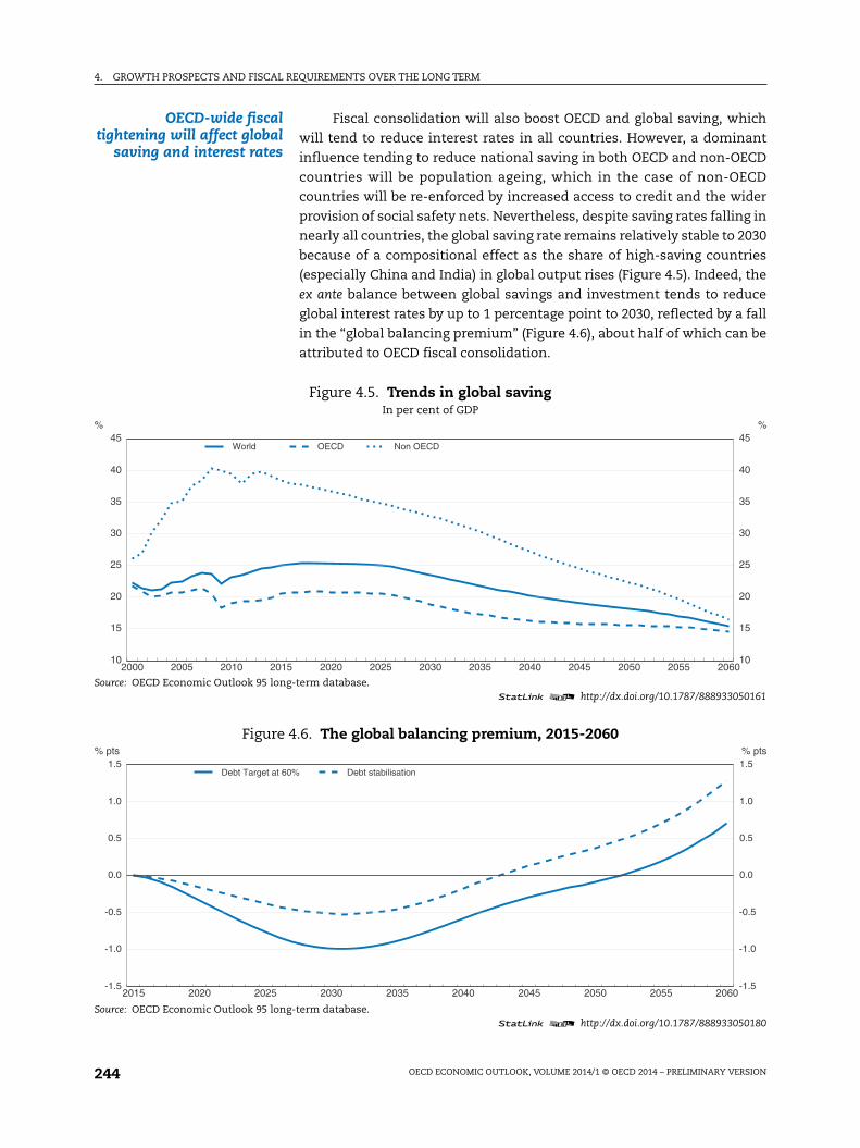
4. GROWTH PROSPECTS AND FISCAL REQUIREMENTS OVER THE LONG TERM
OECD ECONOMIC OUTLOOK, VOLUME 2014/1 © OECD 2014 – PRELIMINARY VERSION244
OECD-wide fiscaltightening will affect global
saving and interest rates
Fiscal consolidation will also boost OECD and global saving, which
will tend to reduce interest rates in all countries. However, a dominant
influence tending to reduce national saving in both OECD and non-OECD
countries will be population ageing, which in the case of non-OECD
countries will be re-enforced by increased access to credit and the wider
provision of social safety nets. Nevertheless, despite saving rates falling in
nearly all countries, the global saving rate remains relatively stable to 2030
because of a compositional effect as the share of high-saving countries
(especially China and India) in global output rises (Figure 4.5). Indeed, the
ex ante balance between global savings and investment tends to reduce
global interest rates by up to 1 percentage point to 2030, reflected by a fall
in the “global balancing premium” (Figure 4.6), about half of which can be
attributed to OECD fiscal consolidation.
Figure 4.5. Trends in global savingIn per cent of GDP
Source: OECD Economic Outlook 95 long-term database.1 2 http://dx.doi.org/10.1787/888933050161
Figure 4.6. The global balancing premium, 2015-2060
Source: OECD Economic Outlook 95 long-term database.1 2 http://dx.doi.org/10.1787/888933050180
2000 2005 2010 2015 2020 2025 2030 2035 2040 2045 2050 2055 206010
15
20
25
30
35
40
45%
10
15
20
25
30
35
40
45%
World OECD Non OECD
2015 2020 2025 2030 2035 2040 2045 2050 2055 2060-1.5
-1.0
-0.5
0.0
0.5
1.0
1.5% pts
-1.5
-1.0
-0.5
0.0
0.5
1.0
1.5% pts
Debt Target at 60% Debt stabilisation

4. GROWTH PROSPECTS AND FISCAL REQUIREMENTS OVER THE LONG TERM
OECD ECONOMIC OUTLOOK, VOLUME 2014/1 © OECD 2014 – PRELIMINARY VERSION 245
Demographic trends maydominate long-run global
saving and interest ratetrends
Beyond 2030, however, the country compositional effect is out-weighed
by the trend decline in saving rates in all countries, and there is a switch in
the direction of the premium. By the 2050s, it has moved from an anticipated
global ex ante saving glut towards a growing global saving shortage, which
puts progressively upward pressure on global interest rates, raising them by
about ¾ of a percentage point in 2060. This projection is, however,
particularly sensitive to developments in China and India (because together
they account for more than one-third of global saving) as well as to the
magnitude of the demographic influence on saving.11
Consolidation boostsmedium-term growth
Apart from improving resilience to cope with future shocks, OECD-
wide fiscal consolidation would boost saving and lower interest rates as
illustrated by comparison with an alternative variant in which OECD fiscal
policy is directed to stabilise government debt only at 2013 levels (Table 4.6).
11. In the model, demographic effects on saving are captured by fixed age-dependency rates, although this creates some tension where retirement agesare increasing, and particularly beyond 2030 when it is assumed thatretirement ages rise in line with life expectancy for all countries.
Table 4.6. The effects of lowering government debt to 60% of GDP
1 2 http://dx.doi.org/10.1787/888933051795
In 2030, or when debt target achieved if later
Public debt
premium
External debt
premium
Government
debt service
GDP growth
2016-30
% pts % pts % of GDP % pts
Austria -0.2 0.0 -1.2 0.1 Belgium -0.5 -0.2 -2.0 0.1 Canada -0.4 -0.2 -2.0 0.1 Czech Republic 0.0 0.0 -0.3 0.0 Denmark 0.0 0.0 -0.2 0.1 Estonia 0.0 0.1 0.0 0.0 Finland 0.0 0.0 -0.6 0.1 France -0.8 -0.3 -3.2 0.2 Germany -0.1 0.0 -0.9 0.1 Greece -3.8 -0.9 -12.8 0.6 Hungary -0.3 0.0 -1.8 0.1 Iceland -0.3 -0.2 -2.5 0.1 Ireland -1.1 -0.2 -3.6 0.2 Italy -1.9 -0.4 -5.7 0.3 Japan -1.3 -0.9 -10.8 0.1 Korea 0.0 0.0 -0.1 0.1 Luxembourg 0.0 0.0 0.0 0.0 Netherlands -0.3 0.0 -1.3 0.1 New Zealand 0.0 0.0 -0.1 0.0 Portugal -1.5 -0.3 -5.1 0.3 Slovak Republic 0.0 0.1 -0.1 0.1 Slovenia -0.2 0.0 -1.3 0.1 Spain -0.7 0.0 -2.5 0.2 Sweden 0.0 0.0 -0.1 0.1 Switzerland 0.0 0.0 -0.1 0.0 United Kingdom -0.7 -0.4 -3.7 0.1 United States -0.6 0.0 -2.6 0.1
Source: OECD Economic Outlook 95 long-term database.
Note: Table shows the effect of reducing government debt to 60% of GDP compared to an alternative counter- factual in which fiscal policy is directed towards stabilising government debt at 2013 levels.

4. GROWTH PROSPECTS AND FISCAL REQUIREMENTS OVER THE LONG TERM
OECD ECONOMIC OUTLOOK, VOLUME 2014/1 © OECD 2014 – PRELIMINARY VERSION246
Reducing government debt to 60% of GDP would, for the 10 OECD
countries for which government debt is currently highest, lower
combined fiscal and net external debt risk premia by an average of 1½
percentage points, reduce government debt service by an average of 4
percentage points of GDP and boost medium-term growth by 0.2
percentage points per year (all by 2030, relative to a counter-factual in
which current debt levels are maintained). This boost to GDP ignores the
Keynesian effects that further consolidation might have in delaying the
closure of output gaps with possible detrimental hysteresis effects on
potential output (De Long and Summers, 2012), although the pace of
further consolidation is assumed to be modest (a maximum of ½ per cent
of GDP per annum).
Global current account imbalances
Fiscal consolidation alsoreduces global imbalances
The overall scale of global current account imbalances, measured as
the absolute sum of all nominal current account balances normalised on
global GDP, is currently around one-third lower than pre-crisis peaks, but
is expected to rise to around 2020, before broadly stabilising to 2030
(Figure 4.7). Given that the majority of OECD countries with high
government debt are also projected to be running current account deficits,
OECD-wide fiscal consolidation will also relieve pressure on global
imbalances. Judged relative to a variant scenario in which OECD fiscal
policy only stabilises government debt at 2013 levels, fiscal consolidation
in the baseline projections reduces global imbalances by up to 15% over
the period to 2030.
Figure 4.7. Global current account imbalances will increase until 2020Sum of absolute current account balances, divided by 2, in per cent of world GDP
Note: 'Government debt stabilisation' is a scenario in which OECD countries target a stable government-debt-to-GDP ratio at currentlevels, rather than reduce it to 60% of GDP as in the baseline.Source: OECD Economic Outlook 95 long-term database.
1 2 http://dx.doi.org/10.1787/888933050199
2000 2005 2010 2015 2020 2025 2030 2035 2040 2045 2050 2055 20600.0
0.5
1.0
1.5
2.0
2.5
3.0
3.5
4.0%
0.0
0.5
1.0
1.5
2.0
2.5
3.0
3.5
4.0%
Baseline Government debt stabilisation
4. GROWTH PROSPECTS AND FISCAL REQUIREMENTS OVER THE LONG TERM
OECD ECONOMIC OUTLOOK, VOLUME 2014/1 © OECD 2014 – PRELIMINARY VERSION 247
The effect of structural reforms on employment, growthand fiscal positions
There is substantial scopefor further structural
improvements
A recent survey of structural performance of OECD and BRIICS
economies (OECD, 2014b) called for “ambitious and comprehensive
structural reform” to facilitate a return to healthy and sustainable growth.
Structural reforms, particularly if they boost employment, can also ease
fiscal constraints. While some structural reform is built into the current
projection baseline, there remains ample scope for further enhancement
as illustrated in a range of scenarios considered here: firstly, raising
potential employment, either by reducing structural unemployment or
promoting female labour force participation; secondly, improving product
market regulation to facilitate competition and so boost productivity; and
finally to promote human capital by better access to quality education.
The fiscal effects of higher potential employment
Lower structuralunemployment relieves
fiscal pressures
In a reform scenario, labour market reforms are assumed to reduce
structural unemployment to 5% in all OECD countries where it currently
exceeds this level.12 Higher potential employment increases tax revenue
and reduces unemployment-related welfare benefits. Furthermore, if the
additional employment is in the private sector, implying a rise in the tax
base relative to expenditure on public sector wages, then total
government expenditure will fall as a share of GDP.13 On this basis, the
scope for the largest falls in structural unemployment relative to the
baseline projection are for Spain (down by 10 percentage points), Greece
(7½ percentage points), the Slovak Republic (9 percentage points) and
Portugal (4 percentage points). The biggest permanent improvements in
the primary balance are for these countries as well as others, such as
France or Belgium, for which the fall in structural unemployment may be
less, but unemployment-related benefits are relatively high and public
sector employment is a relatively high share of total employment
(Figure 4.8). For these six countries, the reduction in structural
unemployment would permanently improve the primary balance by more
than 2 percentage points of GDP and for Spain the improvement would be
more than double that. To put the magnitude of these effects in context,
the pressures from increased public spending on health and pensions are
expected to amount to just under 3 percentage points of GDP for the
median OECD country to 2030. As well as reducing the extent of required
12. A structural unemployment rate of 5% was achieved by almost one-third ofOECD countries in the immediate pre-crisis period. In the baseline projection,structural unemployment is slowly converging to the level observed before thecrisis in each country.
13. Structural reforms are more likely to positively affect fiscal balances if theygenerate higher potential employment rather than result in higher trendproductivity. The total estimated improvement in the underlying primarybalance from an increase in potential employment by 1 percentage point rangesfrom between 0.3 and 0.8 per cent of GDP, with the effect largest in countrieswhere the initial ratio of public to private sector employment and the initialproportion of primary public expenditure to GDP are highest (OECD, 2010).

4. GROWTH PROSPECTS AND FISCAL REQUIREMENTS OVER THE LONG TERM
OECD ECONOMIC OUTLOOK, VOLUME 2014/1 © OECD 2014 – PRELIMINARY VERSION248
consolidation to achieve any given debt target, falling structural
unemployment would also enable that target to be achieved earlier;14 the
60% debt target in the baseline would be reached 5 years earlier for the
Slovak Republic, 4 years earlier for Greece and 3 years earlier for France
and Portugal.
Promoting femaleparticipation should be a
priority in manycountries…
Raising the participation of women should be a structural policy
priority, particularly for countries in which rapidly ageing populations are
most likely to be a drag on the employment rate (OECD, 2013b and 2014b).
While social trends have played a key role in the rise in female
participation, policies can also have an impact (Thévenon, 2013). This is
particularly true as regards the availability of reliable and affordable day-
care, which significantly increases the ability of either spouse to remain in
the workforce after child-birth – but most often impacts on women. A
related issue is whether parental leave that can be taken by either parent.
Other policies that have significant impacts on female participation
include facilitating part-time employment, which at present is still
subject to significant penalties relative to full-time employment in most
countries (OECD, 2010), including lack of basic levels of job security,
training and promotion, less access to unemployment benefits or re-
employment assistance.
Figure 4.8. The fiscal gains from a fall in structural unemploymentChange in the underlying primary balance compared to the baseline, percentage points of GDP
Note: The numbers represent the effect on the primary balance of a fall of the structural unemployment to 5 per cent. Countries whereunemployment is already below 5 per cent are not shown.Source: OECD Economic Outlook 95 long-term database; and OECD Calculations.
1 2 http://dx.doi.org/10.1787/888933050218
0.0
0.5
1.0
1.5
2.0
2.5
3.0
3.5
4.0
4.5
5.0% pts
0.0
0.5
1.0
1.5
2.0
2.5
3.0
3.5
4.0
4.5
5.0% pts
ES
P
SV
K
GR
C
FR
A
PO
L
BE
L
HU
N
PR
T
FIN IRL
SW
E
ITA
CA
N
DE
U
CZ
E
GB
R
US
A
AU
S
DN
K
14. Fiscal consolidation in the baseline takes place through a gradual improvementin the underlying primary balance with a maximum cap on consolidation inany single year of ½ percentage point of GDP, but the effect from the reductionin unemployment is assumed to come in addition to the cap as theimprovement is an indirect effect of labour market reforms.
4. GROWTH PROSPECTS AND FISCAL REQUIREMENTS OVER THE LONG TERM
OECD ECONOMIC OUTLOOK, VOLUME 2014/1 © OECD 2014 – PRELIMINARY VERSION 249
… and the gains could belarge for some countries
In a further variant scenario, the participation rate of women in 2030
is raised to that of the full-time equivalent currently prevailing in the
median OECD country (54%). For Turkey, Poland and Italy this results in
aggregate participation gains large enough to increase GDP by over 10% in
2030. Increases of 5% or more also result for Belgium, the Czech Republic,
France, Greece, Hungary and Japan. Given the likely boost to private
employment, this could also deliver substantial fiscal savings; estimated to
be about 6% of GDP for Italy and Poland; and 2-3% of GDP for Belgium, the
Czech Republic, France, Greece, Hungary, Japan and the Slovak Republic.15
The growth effects of product market reforms
A faster pace of productmarket reform would boost
GDP
There is a substantial body of evidence at the firm, industry and
macro-level, linking competition-friendly product market regulation (as
quantified by the OECD’s PMR index) with better productivity
performance, a link which is embodied in the modelling framework
underlying the current projections.16 In the baseline scenario, a gradual
improvement in product market regulations (as quantified by the PMR
index) is assumed so that all countries improve to at least the current
average across OECD countries at a speed which is consistent with the
average rate of improvement observed over recent history. This speed of
improvement has slowed over the past 5 years, although there are some
exceptions – notably Greece, Italy, Poland, Portugal and the Slovak
Republic – where there have been more substantial reforms (OECD, 2014b).
In a variant scenario, designed to reflect a faster pace of reform, the rate
of improvement in product market regulations in all countries is set equal
to the average pace of this fast-reforming group of countries. The faster
speed of product market reform boosts trend productivity most in those
countries where there is greatest scope to catch-up in terms of
competition-enhancing regulation (and not at all for those countries for
which the PMR indicator is already better than the current OECD average).
Thus, gains are typically larger for non-OECD economies, with GDP
increasing by an average of 9% by 2030, and for the six OECD countries in
which regulations are currently most stringent, where GDP is boosted by
an average of 6% by 2030 (Figure 4.9). In a further scenario, in which the
level of product market regulation is also assumed to improve to at least
the best quartile currently observed among OECD countries, rather than
just the current OECD average (as in the baseline and first scenario), the
15. The fiscal savings from higher female participation could be offset if there weresignificant fiscal costs from higher public support for child-care needed to bringthis about.
16. A link between firm, industry and macro-level growth performance andcompetition-enhancing product market regulation is found by Bourlès et al.(2010), Bouis et al. (2011), Conway, et al. (2006) and Griffith, et al. (2004). In theempir ica l work under ly ing the current model l ing framework(Johansson et al., 2013) more pro-competition product market regulation, asquantified by the OECD’s product market regulation index, was found to boostlong-term productivity and thus affect the pace at which countries convergetowards the international technological frontier.

4. GROWTH PROSPECTS AND FISCAL REQUIREMENTS OVER THE LONG TERM
OECD ECONOMIC OUTLOOK, VOLUME 2014/1 © OECD 2014 – PRELIMINARY VERSION250
GDP gains would be even larger and spread among a much wider group of
countries. Such a reform effort would also come close to meeting the G20’s
target to raise collective GDP by 2% within 5 years.
The gains from improving access to education in emerging market economies
Education reforms inemerging market economiescould boost human capital
Improving access to quality education is a priority recommendation
in many emerging economies, including the BRIICS, as well as Turkey,
Mexico and Chile (OECD, 2013b and 2014b). Education increases human
capital and so makes workers more productive and has been among the
most important drivers for increasing long-run living standards (Cohen
and Soto, 2007; Bouis et al, 2011). There is likely to be a larger benefit to
reforms where average years of schooling are initially low, as empirical
evidence suggests that the returns from boosting coverage and
performance in primary and secondary education are greater than for
tertiary education.17 In order to simulate the effect of ambitious education
reforms in emerging economies, a variant scenario with faster
improvement in educational attainment was constructed based on
historical episodes in low-income countries in which major reforms
enhanced primary and secondary coverage and performance. Brazil,
Chile, Indonesia, Korea, Mexico, and Russia all experienced periods of a
decade or more in which there was above average growth in educational
Figure 4.9. The effect of improved product market regulation on GDPIn 2030, per cent
Note: The 'Faster pace' shows the effect of an increase in the speed of product market reform which roughly matches the average rate ofimprovement in the PMR index observed over the period 2008-13 for Greece, Italy, Poland, Portugal and Slovak Republic. The 'Faster paceof reform to best practice' shows the effect of the same increased speed of product market reform, but to a level which matches thecurrent best quartile among OECD countries rather than the current OECD average as in the baseline and first scenario.Source: OECD Economic Outlook 95 long-term database; and OECD Calculations.
1 2 http://dx.doi.org/10.1787/888933050237
0
2
4
6
8
10
12
14
16
18
20
22%
0
2
4
6
8
10
12
14
16
18
20
22%
FIN
PR
T
HU
N
SV
K
ES
T
CA
N
CZ
E
FR
A
BE
L
ES
P
JPN
CH
L
ISL
NO
R
CH
E
IRL
ME
X
SW
E
GR
C
BR
A
LUX
KO
R
SV
N
ZA
F
TU
R
PO
L
ISR
IDN
IND
RU
S
CH
N
Faster paceFaster pace to best practice
17. This is reflected in the current modelling framework whereby human capitalimprovement is modelled as a decreasing function of additional years ofschooling

4. GROWTH PROSPECTS AND FISCAL REQUIREMENTS OVER THE LONG TERM
OECD ECONOMIC OUTLOOK, VOLUME 2014/1 © OECD 2014 – PRELIMINARY VERSION 251
attainment of the 25 to 29 year-old group. During these episodes, the
annual speed of convergence in educational levels was on average around
60% higher than assumed in the baseline. Applying a similar rate of
improvement, the variant scenario highlights the long-term gains in
productivity that faster improvements in educational attainment can
bring in emerging economies. There are likely to be long lags before there
are major GDP effects because the primary beneficiaries will be those who
are currently young, but over the long-term (to 2060) the GDP gains could
be around 10% or more for China, India, Indonesia and South Africa
(Figure 4.10).18
18. The Turkish government recently approved a reform programme aimed atincreasing the average schooling attainment of the cohort age 25 to 29 to about13 years by 2025, which is not incorporated in the baseline projection reportedhere, but the possible effects on GDP are considered in OECD (2012).
Figure 4.10. The effect of improving access to education on GDPPer cent
Note: The bars report the impact on GDP that increased access to quality-education will have through improvements in human capital.Source: OECD Economic Outlook 95 long-term database; and OECD calculations.
1 2 http://dx.doi.org/10.1787/888933050256
0
5
10
15%
0
5
10
15%
IND
CH
N
ZA
F
IDN
RU
S
TU
R
AR
G
BR
A
ME
X
CH
L
Change to 2030Change to 2060

4. GROWTH PROSPECTS AND FISCAL REQUIREMENTS OVER THE LONG TERM
OECD ECONOMIC OUTLOOK, VOLUME 2014/1 © OECD 2014 – PRELIMINARY VERSION252
Bibliography
Bouis, R., R. Duval and F. Murtin (2011), “The Policy and Institutional Drivers ofEconomic Growth Across OECD and Non-OECD Economies: New Evidence fromGrowth Regressions”, OECD Economics Department Working Papers, No. 843, OECDPublishing.
Bourlès, R., G. Cette, J. Lopez, J. Mairesse and G. Nicoletti (2010), “Do Product MarketRegulations in Upstream Sectors Curb Productivity Growth?: Panel DataEvidence for OECD Countries”, OECD Economics Department Working Papers,No. 791, OECD Publishing.
Cohen and Soto (2007), “Growth and Human Capital: Good Data, Good Results”,Journal of Economic Growth, Vol. 12.
Conway, P., D. De Rosa, G. Nicoletti and F. Steiner (2006), “Regulation, Competitionand Productivity Convergence”, OECD Economics Department Working Paper,No. 509, OECD Publishing.
DeLong, B. and L. Summers (2012), “Fiscal Policy in a Depressed Economy”, paperprepared for the Spring 2012 Brookings Panel on Economic Activity, 22-23March, Washington, D.C.
Égert, B. (2010), “Fiscal Policy Reaction to the Cycle in the OECD: Pro- or Counter-Cyclical?”, OECD Economics Department Working Papers, No. 763, OECD Publishing.
Frankel, J. (2006), “The Balassa-Samuelson Relationship and the Renminbi”, HarvardWorking Paper, December.
Griffith, R., S. Redding and J. van Reenen (2004), “Mapping the Two Faces of R&D:Productivity Growth in a Panel of OECD Countries”, Review of Economics andStatistics, Vol. 86.
Johansson, A., Y. Guillemette, F. Murtin, D. Turner, G. Nicoletti, C. de laMaisonneuve, P. Bagnoli, G. Bousquet and F. Spinelli (2013), “Long-Term GrowthScenarios”, OECD Economics Department Working Papers, No. 1000, OECDPublishing.
Guillemette, Y. and J. Strasky (2013), “Japan's Challenging Debt Dynamics”, OECDEconomics Department Working Papers, No. 1085, OECD Publishing.
Kerdrain, C., I. Koske and I. Wanner (2010), “The Impact of Structural Policies onSaving, Investment and Current Accounts”, OECD Economics Department WorkingPapers, No. 815, OECD Publishing.
Lane, P. R. and G.M. Milesi Ferreti (2001), “Long-Term Capital Movements”, Center forEconomic Policy Research, Discussion paper, No. 2873.
Laubach, T. (2009), “New Evidence on the Interest Rate Effects of Budget Deficits andDebt”, Journal of the European Economic Association, Vol. 7.
OECD (2010), Economic Outlook No. 88, “Fiscal Consolidation Requirements, Timing,Instruments and Institutional arrangements”, Chapter 4, OECD Publishing.
OECD (2012), OECD Economic Surveys: Turkey, OECD Publishing.
OECD (2013a), Economic Outlook No. 93, “Growth Prospects and Fiscal Requirementsover the Long Term”, Chapter 4, OECD Publishing.
OECD (2013b), Economic Policy Reforms, Going for Growth, OECD Publishing.
OECD (2014a), “OECD@100: Policies for a Shifting World”, OECD Economic PolicyPapers, forthcoming, OECD Publishing.
OECD (2014b), Economic Policy Reforms, Going For Growth, Interim Report, 2014, OECDPublishing.
Oliveira Martins, J. and C. de la Maisonneuve (2014, forthcoming), “The Future ofHealth and Long-Term Care Spending”, OECD Economic Studies, OECD Publishing.
Röhn, O. (2011), “New Evidence on the Private Saving Offset and RicardianEquivalence”, OECD Economics Department Working Paper, No. 762, OECD Publishing.
Rose, D. (2010), “The Influence of Foreign Assets and Liabilities on Real InterestRates”, Institute of Policy Studies Working Paper 10/09.

4. GROWTH PROSPECTS AND FISCAL REQUIREMENTS OVER THE LONG TERM
OECD ECONOMIC OUTLOOK, VOLUME 2014/1 © OECD 2014 – PRELIMINARY VERSION 253
Thévenon, O. (2013), “Drivers of Female Labour Force Participation in the OECD”,OECD Social, Employment and Migration Working Paper, No. 145, OECD Publishing.
Turner, D. and F. Spinelli (2013), “The effect of government debt, external debt andtheir interaction on OECD interest rates”, OECD Economics Department WorkingPaper, No. 1103, OECD Publishing.