1

GROUND WATER POLLUTION POTENTIAL ASHTABULA COUNTY, OHIO

BY

LINDA ALLER AND KAREN BALLOU

GEODYSSEY, INC.

1991

REVISED BY

KATHY SPROWLS

2012

GROUND WATER POLLUTION POTENTIAL REPORT NO. 10

OHIO DEPARTMENT OF NATURAL RESOURCES

DIVISION OF SOIL AND WATER RESOURCES

WATER RESOURCES SECTION

ii

ABSTRACT

A ground water pollution potential mapping program for Ohio has been developed under the direction of the Division of Water (now Soil and Water Resources), Ohio Department of Natural Resources, using the DRASTIC mapping process. The DRASTIC system consists of two major elements: the designation of mappable units, termed hydrogeologic settings, and the superposition of a relative rating system for pollution potential.

Hydrogeologic settings form the basis of the system and incorporate the major hydrogeologic factors that affect and control ground water movement and occurrence including depth to water, net recharge, aquifer media, soil media, topography, impact of the vadose zone media, and hydraulic conductivity of the aquifer. These factors, which form the acronym DRASTIC, are incorporated into a relative ranking scheme that uses a combination of weights and ratings to produce a numerical value called the ground water pollution potential index. Hydrogeologic settings are combined with the pollution potential indexes to create units that can be graphically displayed on a map.

Ashtabula County lies within the Glaciated Central Region. The county is covered by variable thicknesses of glacial lake deposits, tills and outwash. In the northern portion of the county, areas of glacial lake deposits have a moderate vulnerability to contamination. In areas of glacial till over bedrock, pollution potential indexes range from low to moderate. Buried valleys containing sand and gravel deposits, and areas of outwash have moderately high to high vulnerability to contamination. Beach ridges, swamps and areas of alluvium adjacent to rivers throughout the county exhibit a moderate to high pollution potential. Nine hydrogeologic settings were identified in Ashtabula County with computed ground water pollution potential indexes ranging from 90 to 207.

The ground water pollution potential mapping program optimizes the use of existing data to rank areas with respect to relative vulnerability to contamination. The ground water pollution potential map of Ashtabula County has been prepared to assist planners, managers, and local officials in evaluating the potential for contamination from various sources of pollution. This information can be used to help direct resources and land use activities to appropriate areas, or to assist in protection, monitoring and clean-up efforts.

iii

 TABLE  OF  CONTENTS  

       

ABSTRACT .................................................................................................................... ii  TABLE OF CONTENTS ............................................................................................... iii  LIST  OF  FIGURES ......................................................................................................... iv  LIST OF TABLES ........................................................................................................... v  ACKNOWLEDGEMENTS ........................................................................................... vi  INTRODUCTION ......................................................................................................... 1  APPLICATIONS OF POLLUTION POTENTIAL MAPS ........................................ 2  SUMMARY OF THE DRASTIC MAPPING PROCESS ........................................... 4  

Hydrogeologic Settings and Factors .............................................................. 4  Weighting and Rating System ......................................................................... 7  Pesticide DRASTIC ........................................................................................... 8  Integration of Hydrogeologic Settings and DRASTIC Factors .................. 11  

INTERPRETATION AND USE OF A GROUND WATER POLLUTION POTENTIAL MAP ........................................................................................... 11  

GENERAL INFORMATION ABOUT ASHTABULA COUNTY ........................... 14  Demographics .................................................................................................... 14  Physiography ..................................................................................................... 14  Glacial Geology ................................................................................................. 16  Buried Valleys ................................................................................................... 19  Bedrock Geology ............................................................................................... 19  Hydrogeology .................................................................................................... 21  

REFERENCES ................................................................................................................ 23  UNPUBLISHED  DATA ................................................................................................ 26  APPENDIX A Description of the Logic in Factor Selection .................................... 27  APPENDIX B Description of Hydrogeologic Settings and Charts ....................... 31  

iv

LIST  OF  FIGURES  

   

Figure  1.  Format  and  description  of  the  hydrogeologic  setting  -­‐‑  7Aa  Glacial  Till  Over  Bedded  Sedimentary  Rocks.  .................................................................................................  6  Figure  2.  Description  of  the  hydrogeologic  setting  7Aa1  Glacial  Till  Over  Bedded  Sedimentary  Rocks.  .............................................................................................................  13  Figure  3.  Location  map  of  Ashtabula  County.  .................................................................  15    

v

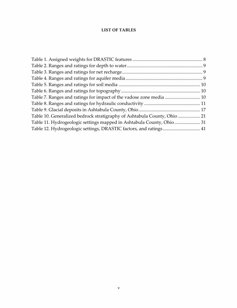
LIST OF TABLES

Table  1.  Assigned  weights  for  DRASTIC  features  ............................................................  8  Table  2.  Ranges  and  ratings  for  depth  to  water  .................................................................  9  Table  3.  Ranges  and  ratings  for  net  recharge  .....................................................................  9  Table  4.  Ranges  and  ratings  for  aquifer  media  ..................................................................  9  Table  5.  Ranges  and  ratings  for  soil  media  ......................................................................  10  Table  6.  Ranges  and  ratings  for  topography  ....................................................................  10  Table  7.  Ranges  and  ratings  for  impact  of  the  vadose  zone  media  ..............................  10  Table  8.  Ranges  and  ratings  for  hydraulic  conductivity  ................................................  11  Table  9.  Glacial  deposits  in  Ashtabula  County,  Ohio  .....................................................  17  Table  10.  Generalized  bedrock  stratigraphy  of  Ashtabula  County,  Ohio  ...................  21  Table  11.  Hydrogeologic  settings  mapped  in  Ashtabula  County,  Ohio  ......................  31  Table  12.  Hydrogeologic  settings,  DRASTIC  factors,  and  ratings  ................................  41  

vi

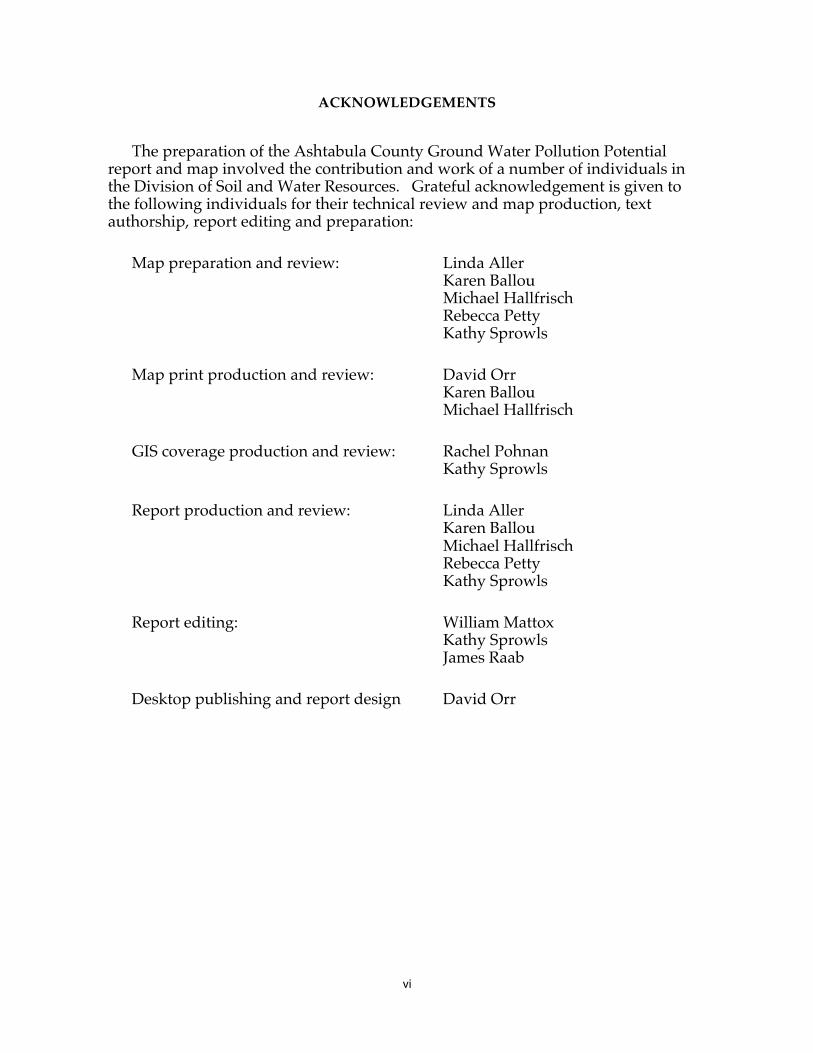
ACKNOWLEDGEMENTS

The preparation of the Ashtabula County Ground Water Pollution Potential report and map involved the contribution and work of a number of individuals in the Division of Soil and Water Resources. Grateful acknowledgement is given to the following individuals for their technical review and map production, text authorship, report editing and preparation:

Map preparation and review: Linda Aller Karen Ballou Michael Hallfrisch Rebecca Petty Kathy Sprowls

Map print production and review: David Orr Karen Ballou Michael Hallfrisch

GIS coverage production and review: Rachel Pohnan Kathy Sprowls

Report production and review: Linda Aller Karen Ballou Michael Hallfrisch Rebecca Petty Kathy Sprowls

Report editing: William Mattox Kathy Sprowls James Raab

Desktop publishing and report design David Orr

1

INTRODUCTION

The need for protection and management of ground water resources in Ohio has been clearly recognized. Approximately 42 per cent of Ohio citizens rely on ground water for their drinking and household uses from both municipal and private wells. Industry and agriculture also utilize significant quantities of ground water for processing and irrigation. In Ohio, over 750,000 rural households depend on private wells; approximately 11, 694 of these wells exist in Ashtabula County.

The characteristics of the many aquifer systems in the state make ground water highly vulnerable to contamination. Measures to protect ground water from contamination usually cost less and create less impact on ground water users than clean up of a polluted aquifer. Based on these concerns for protection of the resource, staff of the Division of Water (now Division of Soil and Water Resources) conducted a review of various mapping strategies useful for identifying vulnerable aquifer areas. They placed particular emphasis on reviewing mapping systems that would assist in state and local protection and management programs. Based on these factors and the quantity and quality of available data on ground water resources, the DRASTIC mapping process (Aller et al., 1987) was selected for application in the program.

Considerable interest in the mapping program followed successful production of a demonstration county map and led to the inclusion of the program as a recommended initiative in the Ohio Ground Water Protection and Management Strategy (Ohio EPA, 1986). Based on this recommendation, the Ohio General Assembly funded the mapping program. A dedicated mapping unit has been established in the Division of Soil and Water Resources, Water Resources Section to implement the ground water pollution potential mapping program on a county-wide basis in Ohio.

The purpose of this report and map is to aid in the protection of our ground water resources. This protection can be enhanced partly by understanding and implementing the results of this study which utilizes the DRASTIC system of evaluating an area's potential for ground-water pollution. The mapping program identifies areas that are more or less vulnerable to contamination and displays this information graphically on maps. The system was not designed or intended to replace site-specific investigations, but rather to be used as a planning and management tool. The results of the map and report can be combined with other information to assist in prioritizing local resources and in making land use decisions.

2

APPLICATIONS OF POLLUTION POTENTIAL MAPS

The pollution potential mapping program offers a wide variety of applications in many counties. The ground water pollution potential map of Ashtabula County was prepared to assist planners, managers, and state and local officials in evaluating the relative vulnerability of areas to ground-water contamination from various sources of pollution. This information can be used to help direct resources and land use activities to appropriate areas, or to assist in protection, monitoring and clean-up efforts.

An important application of the pollution potential maps for many areas will be to assist in county land use planning and resource expenditures related to solid waste disposal. A county may use the map to help identify areas that are more or less suitable for land disposal activities. Once these areas are identified, a county can collect more site-specific information and combine this with other local factors to determine site suitability.

A pollution potential map can also assist in developing ground-water protection strategies. By identifying areas more vulnerable to contamination, officials can direct resources to areas where special attention or protection efforts might be warranted. This information can be utilized effectively at the local level for integration into land use decisions and as an educational tool to promote public awareness of ground water resources. Pollution potential maps may also be used to prioritize ground water monitoring and/or contamination clean-up efforts. Areas that are identified as being vulnerable to contamination may benefit from increased ground water monitoring for pollutants or from additional efforts to clean up an aquifer.

Pollution potential maps may also be applied successfully where non-point source contamination is a concern. Non-point source contamination occurs where land use activities over large areas impact water quality. Maps providing information on relative vulnerability can be used to guide the selection and implementation of appropriate best management practices in different areas. Best management practices should be chosen based upon consideration of the chemical and physical processes that occur from the practice, and the effect these processes may have in areas of moderate to high vulnerability to contamination. For example, the use of agricultural best management practices that limit the infiltration of nitrates, or promote denitrification above the water table, would be beneficial to implement in areas of relatively high vulnerability to contamination.

Other beneficial uses of the pollution potential maps will be recognized by individuals in the county who are familiar with specific land use and management problems. Planning commissions and zoning boards can use these maps to help make informed decisions about the development of areas within their jurisdiction. Developments proposed to occur within ground-water sensitive areas may be required to show how ground water will be protected.

3

Regardless of the application, emphasis must be placed on the fact that the system is not designed to replace a site-specific investigation. The strength of the system lies in its ability to make a "first-cut approximation" by identifying areas that are vulnerable to contamination. Any potential applications of the system should also recognize the assumptions inherent in the system.

4

SUMMARY OF THE DRASTIC MAPPING PROCESS

The system chosen for implementation of a ground water pollution potential mapping program in Ohio, DRASTIC, was developed by the National Water Well Association (now National Ground Water Association) for the United States Environmental Protection Agency. A detailed discussion of this system can be found in Aller et al. (1987).

The DRASTIC mapping system allows the pollution potential of any area to be evaluated systematically using existing information. The vulnerability of an area to contamination is a combination of hydrogeologic factors, anthropogenic influences and sources of contamination in any given area. The DRASTIC system focuses only on those hydrogeologic factors which influence ground water pollution potential. The system consists of two major elements: the designation of mappable units, termed hydrogeologic settings, and the superposition of a relative rating system to determine pollution potential.

The application of DRASTIC to an area requires the recognition of a set of assumptions made in the development of the system. DRASTIC evaluates the pollution potential of an area assuming a contaminant with the mobility of water, introduced at the surface, and flushed into the ground water by precipitation. Most important, DRASTIC cannot be applied to areas smaller than one-hundred acres in size, and is not intended or designed to replace site-specific investigations.

Hydrogeologic Settings and Factors

To facilitate the designation of mappable units, the DRASTIC system used the framework of an existing classification system developed by Heath (1984), which divides the United States into fifteen ground water regions based on the factors in a ground water system that affect occurrence and availability.

Within each major hydrogeologic region, smaller units representing specific hydrogeologic settings are identified. Hydrogeologic settings form the basis of the system and represent a composite description of the major geologic and hydrogeologic factors that control ground water movement into, through and out of an area. A hydrogeologic setting represents a mappable unit with common hydrogeologic characteristics, and, as a consequence, common vulnerability to contamination (Aller et al., 1987).

5

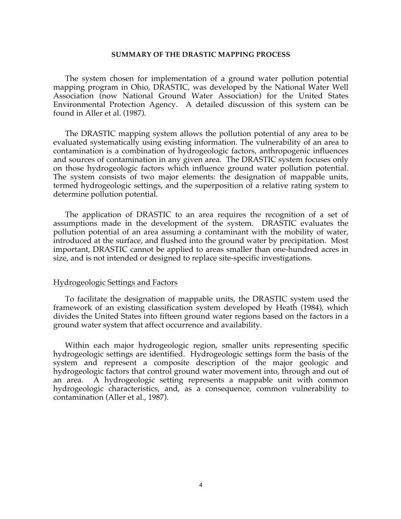
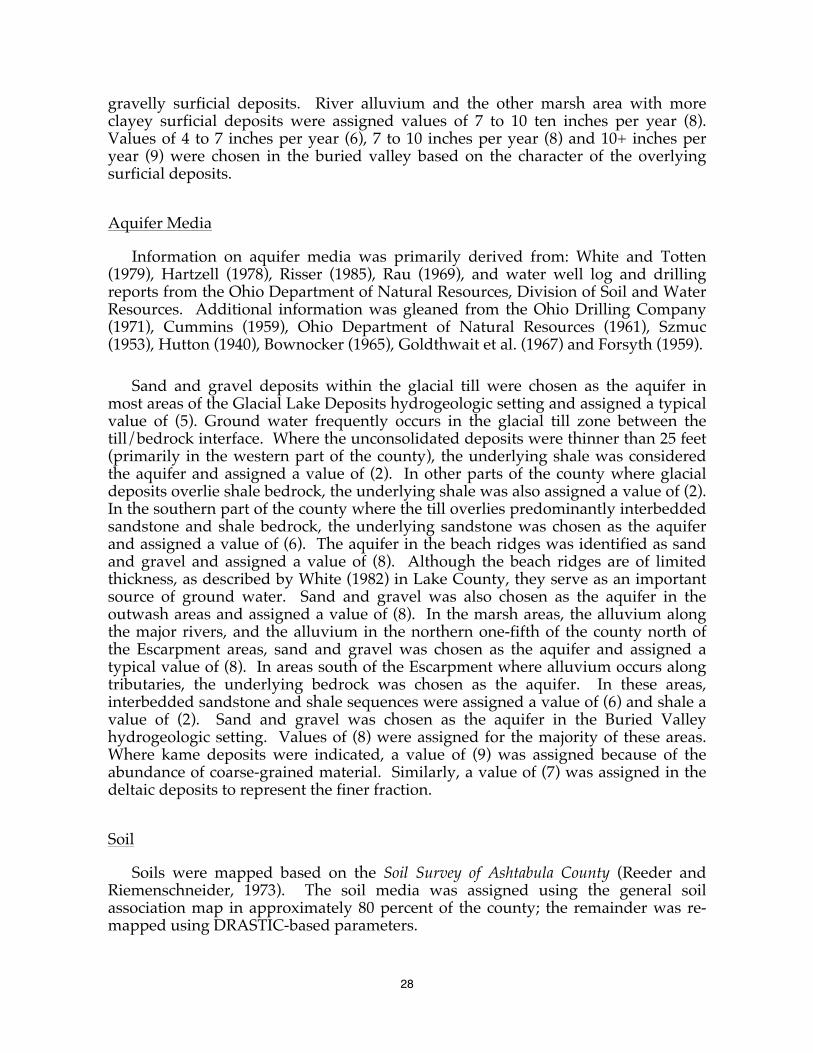
Figure 1 illustrates the format and description of a typical hydrogeologic setting found within Ashtabula County. Inherent within each hydrogeologic setting are the physical characteristics which affect the ground water pollution potential. These characteristics or factors identified during the development of the DRASTIC system include:

D - Depth to Water R - Net Recharge A - Aquifer Media S - Soil Media T - Topography I - Impact of the Vadose Zone Media C - Conductivity (Hydraulic) of the Aquifer These factors incorporate concepts and mechanisms such as attenuation,

retardation and time or distance of travel of a contaminant with respect to the physical characteristics of the hydrogeologic setting. Broad consideration of these factors and mechanisms coupled with existing conditions in a setting provide a basis for determination of the area's relative vulnerability to contamination.

Depth to water is considered to be the depth from the ground surface to the water table in unconfined aquifer conditions or the depth to the top of the aquifer under confined aquifer conditions. The depth to water determines the distance a contaminant would have to travel before reaching the aquifer. The greater the distance the contaminant has to travel the greater the opportunity for attenuation to occur or restriction of movement by relatively impermeable layers.

Net recharge is the total amount of water reaching the land surface that infiltrates into the aquifer measured in inches per year. Recharge water is available to transport a contaminant from the surface into the aquifer and also affects the quantity of water available for dilution and dispersion of a contaminant. Factors to be included in the determination of net recharge include contributions due to infiltration of precipitation, in addition to infiltration from rivers, streams and lakes, irrigation and artificial recharge.

Aquifer media represents consolidated or unconsolidated rock material capable of yielding sufficient quantities of water for use. Aquifer media accounts for the various physical characteristics of the rock that provide mechanisms of attenuation, retardation and flow pathways that affect a contaminant reaching and moving through an aquifer.

6

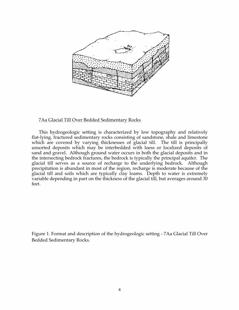
7Aa Glacial Till Over Bedded Sedimentary Rocks

This hydrogeologic setting is characterized by low topography and relatively flat-lying, fractured sedimentary rocks consisting of sandstone, shale and limestone which are covered by varying thicknesses of glacial till. The till is principally unsorted deposits which may be interbedded with loess or localized deposits of sand and gravel. Although ground water occurs in both the glacial deposits and in the intersecting bedrock fractures, the bedrock is typically the principal aquifer. The glacial till serves as a source of recharge to the underlying bedrock. Although precipitation is abundant in most of the region, recharge is moderate because of the glacial till and soils which are typically clay loams. Depth to water is extremely variable depending in part on the thickness of the glacial till, but averages around 30 feet.

Figure  1.  Format  and  description  of  the  hydrogeologic  setting  -­‐‑  7Aa  Glacial  Till  Over  Bedded  Sedimentary  Rocks.  

7

Soil media refers to the upper six feet of the unsaturated zone that is characterized by significant biological activity. The type of soil media can influence the amount of recharge that can move through the soil column due to variations in soil permeability. Various soil types also have the ability to attenuate or retard a contaminant as it moves throughout the soil profile. Soil media is based on textural classifications of soils and considers relative thicknesses and attenuation characteristics of each profile within the soil.

Topography refers to the slope of the land expressed as percent slope. The amount of slope in an area affects the likelihood that a contaminant will run off from an area or be ponded and ultimately infiltrate into the subsurface. Topography also affects soil development and often can be used to help determine the direction and gradient of ground water flow under water table conditions.

Impact of the vadose zone media refers to the attenuation and retardation processes that can occur as a contaminant moves through the unsaturated zone above the aquifer. The vadose zone represents that area below the soil horizon and above the aquifer that is unsaturated or discontinuously saturated. Various attenuation, travel time and distance mechanisms related to the types of geologic materials present can affect the movement of contaminants in the vadose zone. Where an aquifer is unconfined, the vadose zone media represents the materials below the soil horizon and above the water table. Under confined aquifer conditions, the vadose zone is simply referred to as a confining layer. The presence of the confining layer in the unsaturated zone significantly impacts the pollution potential of the ground water in an area.

Hydraulic conductivity of an aquifer is a measure of the ability of the aquifer to transmit water, and is also related to ground water velocity and gradient. Hydraulic conductivity is dependent upon the amount and interconnectivity of void spaces and fractures within a consolidated or unconsolidated rock unit. Higher hydraulic conductivity typically corresponds to higher vulnerability to contamination. Hydraulic conductivity considers the capability for a contaminant that reaches an aquifer to be transported throughout that aquifer over time.

Weighting and Rating System

DRASTIC uses a numerical weighting and rating system that is combined with the DRASTIC factors to calculate a ground water pollution potential index or relative measure of vulnerability to contamination. The DRASTIC factors are weighted from 1 to 5 according to their relative importance to each other with regard to contamination potential (Table 1). Each factor is then divided into ranges

8

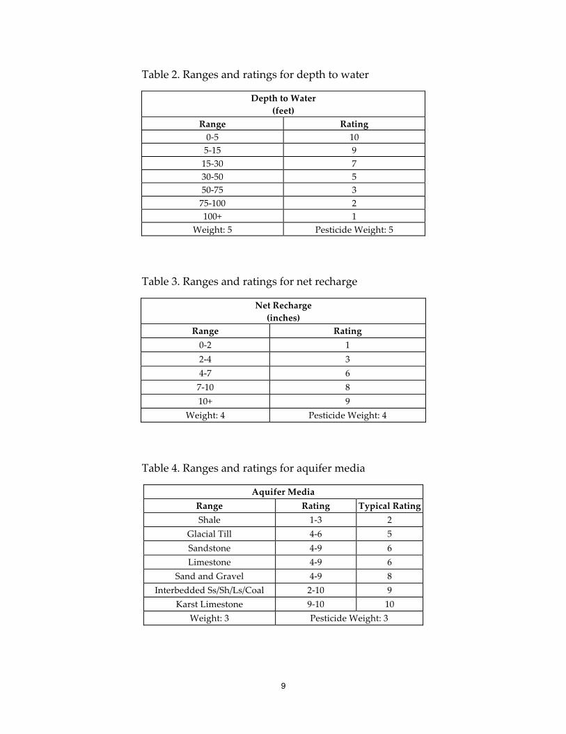
or media types and assigned a rating from 1 to 10 based on their significance to pollution potential (Tables 2-8). The rating for each factor is selected based on available information and professional judgment. The selected rating for each factor is multiplied by the assigned weight for each factor. These numbers are summed to calculate the DRASTIC or pollution potential index.

Once a DRASTIC index has been calculated, it is possible to identify areas that are more likely to be susceptible to ground water contamination relative to other areas. Greater   vulnerability   to   contamination   is   indicated   by   a   higher   DRASTIC  index. The index generated provides only a relative evaluation tool and is not designed to produce absolute answers or to represent units of vulnerability. Pollution potential indexes of various settings should be compared to each other only with consideration of the factors that were evaluated in determining the vulnerability of the area.

Pesticide DRASTIC

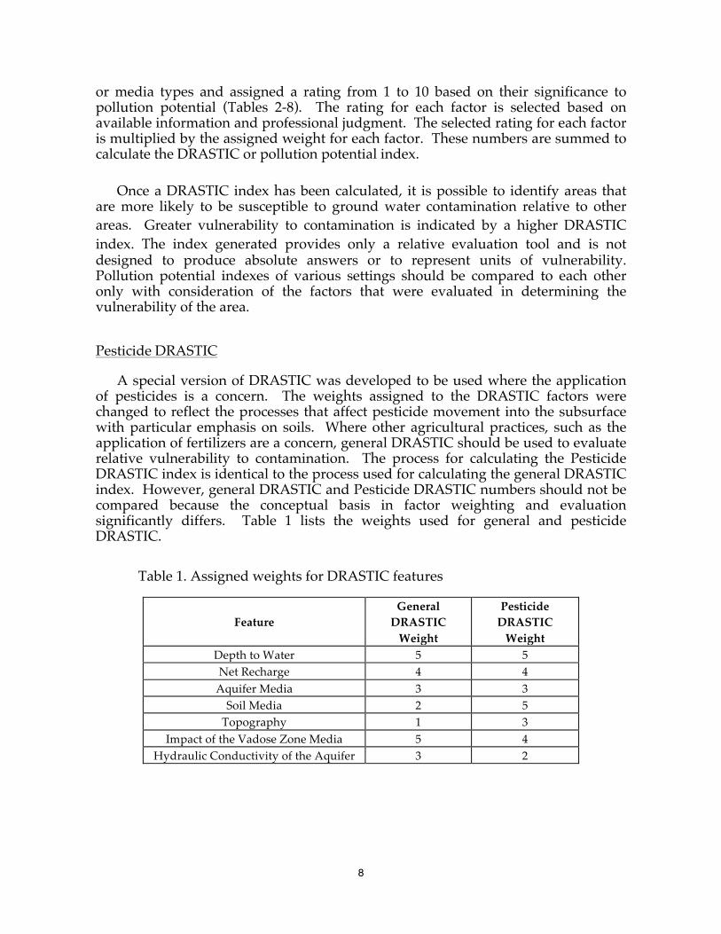
A special version of DRASTIC was developed to be used where the application of pesticides is a concern. The weights assigned to the DRASTIC factors were changed to reflect the processes that affect pesticide movement into the subsurface with particular emphasis on soils. Where other agricultural practices, such as the application of fertilizers are a concern, general DRASTIC should be used to evaluate relative vulnerability to contamination. The process for calculating the Pesticide DRASTIC index is identical to the process used for calculating the general DRASTIC index. However, general DRASTIC and Pesticide DRASTIC numbers should not be compared because the conceptual basis in factor weighting and evaluation significantly differs. Table 1 lists the weights used for general and pesticide DRASTIC.

Table  1.  Assigned  weights  for  DRASTIC  features  

 Feature  

General  DRASTIC  Weight  

Pesticide  DRASTIC  Weight  

Depth  to  Water   5   5  Net  Recharge   4   4  Aquifer  Media   3   3  Soil  Media   2   5  Topography   1   3  

Impact  of  the  Vadose  Zone  Media   5   4  Hydraulic  Conductivity  of  the  Aquifer   3   2  

     

9

Table  2.  Ranges  and  ratings  for  depth  to  water  

Depth  to  Water  (feet)  

Range   Rating  0-­‐‑5   10  5-­‐‑15   9  15-­‐‑30   7  30-­‐‑50   5  50-­‐‑75   3  75-­‐‑100   2  100+   1  

Weight:  5   Pesticide  Weight:  5        

Table  3.  Ranges  and  ratings  for  net  recharge  

Net  Recharge  (inches)  

Range   Rating  0-­‐‑2   1  2-­‐‑4   3  4-­‐‑7   6  7-­‐‑10   8  10+   9  

Weight:  4   Pesticide  Weight:  4        

Table  4.  Ranges  and  ratings  for  aquifer  media  

Aquifer  Media  Range   Rating   Typical  Rating  Shale   1-­‐‑3   2  

Glacial  Till   4-­‐‑6   5  Sandstone   4-­‐‑9   6  Limestone   4-­‐‑9   6  

Sand  and  Gravel   4-­‐‑9   8  Interbedded  Ss/Sh/Ls/Coal     2-­‐‑10   9  

Karst  Limestone   9-­‐‑10   10  Weight:  3   Pesticide  Weight:  3  

   

10

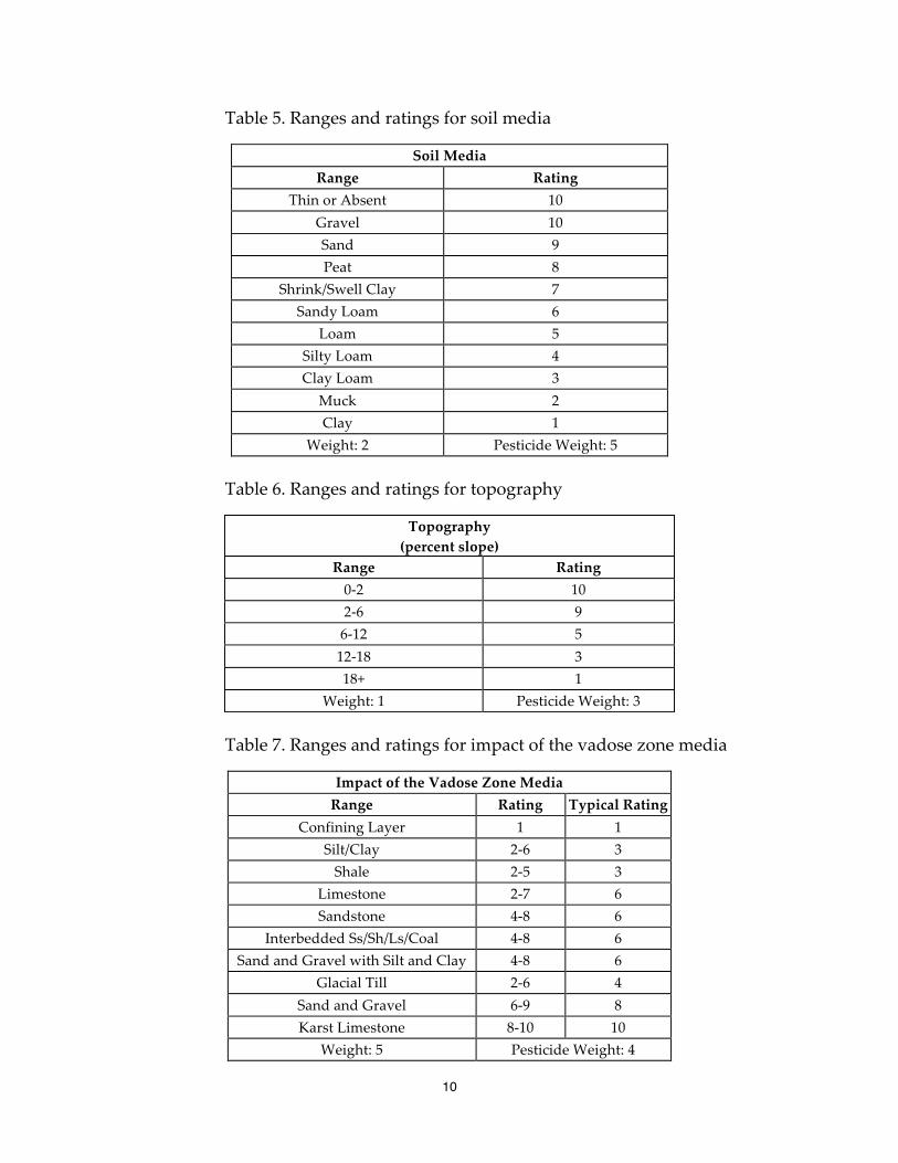
Table  5.  Ranges  and  ratings  for  soil  media  

Soil  Media  Range   Rating  

Thin  or  Absent   10  Gravel   10  Sand   9  Peat   8  

Shrink/Swell  Clay   7  Sandy  Loam   6  

Loam   5  Silty  Loam   4  Clay  Loam   3  

Muck   2  Clay   1  

Weight:  2   Pesticide  Weight:  5             Table  6.  Ranges  and  ratings  for  topography  

Topography  (percent  slope)  

Range   Rating  0-­‐‑2   10  2-­‐‑6   9  6-­‐‑12   5  12-­‐‑18   3  18+   1  

Weight:  1   Pesticide  Weight:  3        

Table  7.  Ranges  and  ratings  for  impact  of  the  vadose  zone  media  

Impact  of  the  Vadose  Zone  Media  Range   Rating   Typical  Rating  

Confining  Layer   1   1  Silt/Clay   2-­‐‑6   3  Shale   2-­‐‑5   3  

Limestone   2-­‐‑7   6  Sandstone   4-­‐‑8   6  

Interbedded  Ss/Sh/Ls/Coal   4-­‐‑8   6  Sand  and  Gravel  with  Silt  and  Clay   4-­‐‑8   6  

Glacial  Till   2-­‐‑6   4  Sand  and  Gravel   6-­‐‑9   8  Karst  Limestone   8-­‐‑10   10  

Weight:  5   Pesticide  Weight:  4    

11

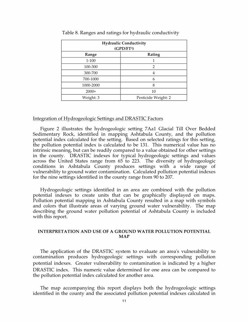
Table  8.  Ranges  and  ratings  for  hydraulic  conductivity  

Hydraulic  Conductivity  (GPD/FT2)  

Range   Rating  1-­‐‑100   1  100-­‐‑300   2  300-­‐‑700   4  700-­‐‑1000   6  1000-­‐‑2000   8  2000+   10  

Weight:  3   Pesticide  Weight:  2  

Integration of Hydrogeologic Settings and DRASTIC Factors

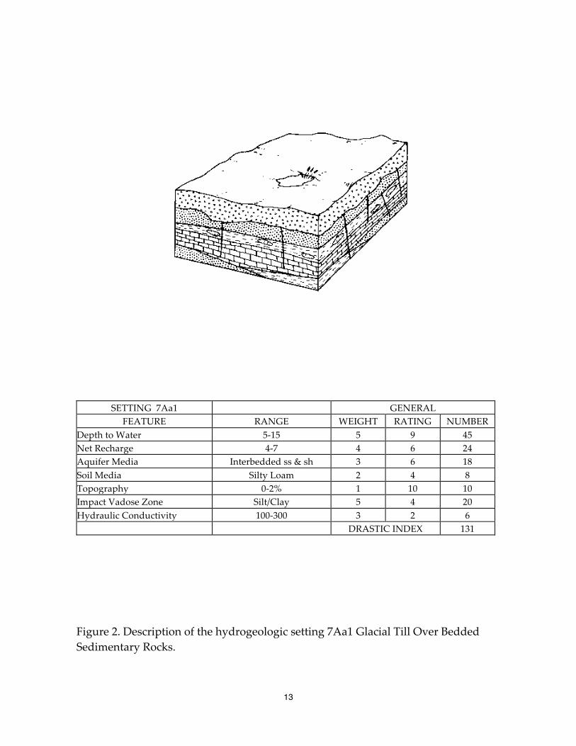
Figure 2 illustrates the hydrogeologic setting 7Aa1 Glacial Till Over Bedded Sedimentary Rock, identified in mapping Ashtabula County, and the pollution potential index calculated for the setting. Based on selected ratings for this setting, the pollution potential index is calculated to be 131. This numerical value has no intrinsic meaning, but can be readily compared to a value obtained for other settings in the county. DRASTIC indexes for typical hydrogeologic settings and values across the United States range from 65 to 223. The diversity of hydrogeologic conditions in Ashtabula County produces settings with a wide range of vulnerability to ground water contamination. Calculated pollution potential indexes for the nine settings identified in the county range from 90 to 207.

Hydrogeologic settings identified in an area are combined with the pollution potential indexes to create units that can be graphically displayed on maps. Pollution potential mapping in Ashtabula County resulted in a map with symbols and colors that illustrate areas of varying ground water vulnerability. The map describing the ground water pollution potential of Ashtabula County is included with this report.

INTERPRETATION AND USE OF A GROUND WATER POLLUTION POTENTIAL MAP

The application of the DRASTIC system to evaluate an area's vulnerability to contamination produces hydrogeologic settings with corresponding pollution potential indexes. Greater   vulnerability   to   contamination   is   indicated  by   a  higher  DRASTIC  index. This numeric value determined for one area can be compared to the pollution potential index calculated for another area.

The map accompanying this report displays both the hydrogeologic settings identified in the county and the associated pollution potential indexes calculated in

12

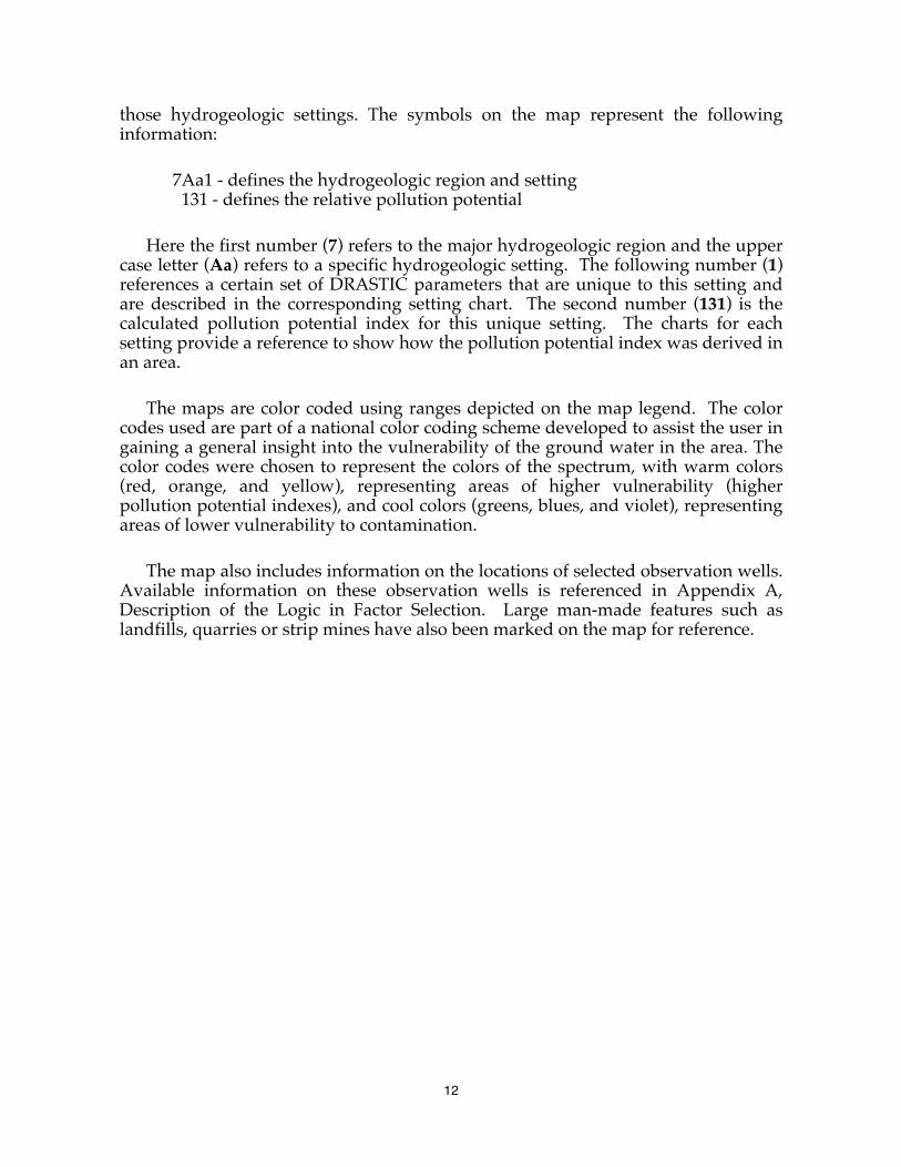
those hydrogeologic settings. The symbols on the map represent the following information:

7Aa1 - defines the hydrogeologic region and setting 131 - defines the relative pollution potential

Here the first number (7) refers to the major hydrogeologic region and the upper case letter (Aa) refers to a specific hydrogeologic setting. The following number (1) references a certain set of DRASTIC parameters that are unique to this setting and are described in the corresponding setting chart. The second number (131) is the calculated pollution potential index for this unique setting. The charts for each setting provide a reference to show how the pollution potential index was derived in an area.

The maps are color coded using ranges depicted on the map legend. The color codes used are part of a national color coding scheme developed to assist the user in gaining a general insight into the vulnerability of the ground water in the area. The color codes were chosen to represent the colors of the spectrum, with warm colors (red, orange, and yellow), representing areas of higher vulnerability (higher pollution potential indexes), and cool colors (greens, blues, and violet), representing areas of lower vulnerability to contamination.

The map also includes information on the locations of selected observation wells. Available information on these observation wells is referenced in Appendix A, Description of the Logic in Factor Selection. Large man-made features such as landfills, quarries or strip mines have also been marked on the map for reference.

13

SETTING    7Aa1     GENERAL  FEATURE   RANGE   WEIGHT   RATING   NUMBER  

Depth  to  Water   5-­‐‑15   5   9   45  Net  Recharge   4-­‐‑7   4   6   24  Aquifer  Media   Interbedded  ss  &  sh   3   6   18  Soil  Media   Silty  Loam   2   4   8  Topography   0-­‐‑2%   1   10   10  Impact  Vadose  Zone   Silt/Clay   5   4   20  Hydraulic  Conductivity   100-­‐‑300   3   2   6       DRASTIC  INDEX   131  

Figure  2.  Description  of  the  hydrogeologic  setting  7Aa1  Glacial  Till  Over  Bedded  Sedimentary  Rocks.  

14

GENERAL INFORMATION ABOUT ASHTABULA COUNTY

Demographics

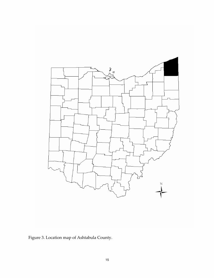
Ashtabula County occupies an area of approximately 705 square miles in the extreme northeast corner of Ohio (Figure 3). It is bounded on the north by Lake Erie, on the east by Pennsylvania, on the south by Trumbull County, and on the west by Lake and Geauga Counties.

The Ashtabula County seat is Jefferson, located near the center of the county, about 55 miles northeast of Cleveland. The 2010 census estimate of the population of Ashtabula County was 101,497 (Ohio Department of Development, 2012).

The average annual precipitation for the city of Ashtabula during the thirty year period starting in 1971 and ending in 2000 was 36.97 inches. The average annual temperature for the same period was 48.4 degrees Fahrenheit (U.S. Department of Commerce, 2002).

Physiography

Ashtabula County lies within two physiographic provinces: the Huron-Erie Lake Plains Section of the Central Lowland Province, and the Glaciated Allegheny Plateaus Section of the Appalachian Plateaus Province (Fenneman, 1938 and Brockman, 1998). The Central Lowland Province occupies a belt 3 to 5.5 miles wide roughly paralleling the lake shore (White and Totten, 1979). This physiographic region typically shows low topography with a gentle slope towards the lake. Ancient beach ridges, left behind by ancient lakes that stood at higher levels than present day Lake Erie, provide the most pronounced surface relief within this province.

The Portage Escarpment that parallels the lake shore separates the Central Lowland Province from the Appalachian Plateaus Province. In Ashtabula County, the Escarpment consists of a belt of bedrock cliffs and glacial end moraines that average 1.5 miles in width and are as wide as 3 miles (White and Totten, 1979).

South of the crest of the Escarpment belt, the topography drops off slightly, then rises gently to a final elevation near 1200 feet (M.S.L.) at the southeastern edge of the county. Relief south of the Escarpment is more pronounced than in the Central Lowland Province. This is particularly true where the major streams flow through steep-walled valleys that are cut deep into the bedrock (White and Totten, 1979).

15

Figure  3.  Location  map  of  Ashtabula  County.  

16

Ashtabula County lies entirely within the Lake Erie drainage basin. The principal streams flowing through the county include Conneaut Creek, the Ashtabula River and the Grand River. In addition, Pymatuning Creek, Rock Creek, and Mill Creek provide a significant portion of the drainage in the county.

Glacial Geology

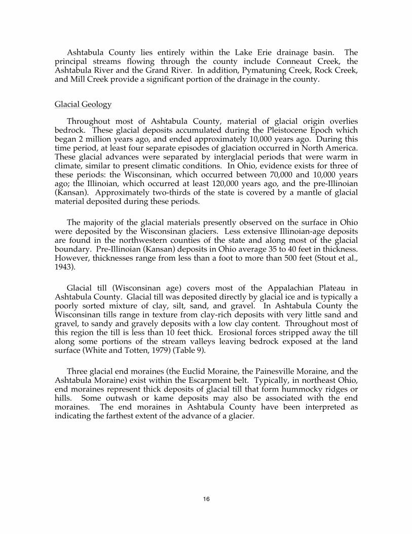
Throughout most of Ashtabula County, material of glacial origin overlies bedrock. These glacial deposits accumulated during the Pleistocene Epoch which began 2 million years ago, and ended approximately 10,000 years ago. During this time period, at least four separate episodes of glaciation occurred in North America. These glacial advances were separated by interglacial periods that were warm in climate, similar to present climatic conditions. In Ohio, evidence exists for three of these periods: the Wisconsinan, which occurred between 70,000 and 10,000 years ago; the Illinoian, which occurred at least 120,000 years ago, and the pre-Illinoian (Kansan). Approximately two-thirds of the state is covered by a mantle of glacial material deposited during these periods.

The majority of the glacial materials presently observed on the surface in Ohio were deposited by the Wisconsinan glaciers. Less extensive Illinoian-age deposits are found in the northwestern counties of the state and along most of the glacial boundary. Pre-Illinoian (Kansan) deposits in Ohio average 35 to 40 feet in thickness. However, thicknesses range from less than a foot to more than 500 feet (Stout et al., 1943).

Glacial till (Wisconsinan age) covers most of the Appalachian Plateau in Ashtabula County. Glacial till was deposited directly by glacial ice and is typically a poorly sorted mixture of clay, silt, sand, and gravel. In Ashtabula County the Wisconsinan tills range in texture from clay-rich deposits with very little sand and gravel, to sandy and gravely deposits with a low clay content. Throughout most of this region the till is less than 10 feet thick. Erosional forces stripped away the till along some portions of the stream valleys leaving bedrock exposed at the land surface (White and Totten, 1979) (Table 9).

Three glacial end moraines (the Euclid Moraine, the Painesville Moraine, and the Ashtabula Moraine) exist within the Escarpment belt. Typically, in northeast Ohio, end moraines represent thick deposits of glacial till that form hummocky ridges or hills. Some outwash or kame deposits may also be associated with the end moraines. The end moraines in Ashtabula County have been interpreted as indicating the farthest extent of the advance of a glacier.

17

Table  9.  Glacial  deposits  in  Ashtabula  County,  Ohio  (after  White  and  Totten,  1979)  

Stage Substage Unit Color

(oxidized)

Color

(unoxidized)

Texture

Wis

cons

inan

Till

Woodfordian

Ashtabula till

Hiram till

Lavery till

Kent till

Brown

Dark brown

Brown

Yellow brown

Gray

Gray

Gray

Gray

Silty, clayey

Clay, few pebbles

Silty, clayey, pebbles

Sandy, coarse

Paleosol

Altonian Titusville till Olive brown Gray Sandy, stony, very hard

? Early Altonian or Illinoian Keefus till Red to red

brown Red to brownish

red Silty, very hard

Pre-

Wis

cons

inan

Till

Unnamed till(s) ? Gray In deep subsurface in

Austinburg, rare elsewhere

18

The Euclid Moraine is the southernmost end moraine within the Escarpment belt. This moraine is a strip of land 1 to 2 miles wide beginning south of the Grand River in eastern Ashtabula County, and extending to south of the Ashtabula River in the western portion of the county. Glacial drift within the moraine ranges from less than 20 to as much as 50 feet in thickness (White and Totten, 1979).

The Painesville Moraine lies north of the Euclid Moraine. This feature extends across the county in a northeasterly direction from northern Harpersfield Township to the Pennsylvania state line. The Painesville Moraine ranges from 1.5 to 2.5 miles wide and exhibits pronounced hummocky topography. Drift thickness within the moraine varies from 30 feet to more than 100 feet, except where it crosses a buried valley in Austinburg Township. At this location the drift is as much as 250 feet thick (White and Totten, 1979).

The Ashtabula Moraine occupies a belt of land, north of the Euclid Moraine, extending from the City of Ashtabula eastward into Pennsylvania. Between the Ashtabula and Conneaut corporation limits, the Moraine has been eroded into individual fragments ranging from 0.25 to 1 mile long. Gaps between the moraine fragments may be as wide as 1.75 miles. East of the Conneaut corporation limit and extending to the Pennsylvania line, the moraine varies from 1.25 to 1.5 miles in width. The surface of the Ashtabula Moraine is hummocky, with some knolls up to 30 feet high (White and Totten, 1979).

South of the Escarpment a fourth end moraine crosses part of Ashtabula County. The Defiance Moraine enters the county in Wayne and Williamsfield Townships and continues almost due north to northwestern Andover Township. At this point the moraine trends northeast to the Pennsylvania state line. The Defiance Moraine varies in width from 4 miles, where it enters the county, to 1.5 miles in parts of Andover and Richmond Townships (White and Totten, 1979).

Outwash deposits, kames and kame terraces are relatively common in the Appalachian Plateau Province of Ashtabula County. These deposits are especially prevalent within the valleys currently occupied by the larger streams that flow through the county (White and Totten, 1979).

As glacial ice melts, a tremendous volume of water is released. This meltwater carries with it sand, gravel, silt and clay previously trapped within the glacial ice. The moving water sorts these materials by size, weight, and shape, depositing the coarse sand and gravel near the source of the meltwater and carrying away the silt and clay downstream. Outwash deposits are formed when sand and gravel is deposited directly on the land surface in front of glacial ice. A kame deposit forms when sand and gravel is deposited directly in holes or depressions on the ice, and subsequently accumulates on the land surface as the ice melts. In areas where ice remained in the valleys while the uplands were ice-free, meltwater deposited sand and gravel accumulated in bands along the margins between the ice and the uplands forming kame terraces.

19

North of the Escarpment, lacustrine (lake bottom) deposits cover most of the Central Lowland Province. Layers of silt and fine sand are the primary components of these deposits. Surface runoff washed these sediments into glacial lakes that covered parts of Ashtabula County prior to the existence of modern Lake Erie. Over a period of time the silt and sand settled to the bottom of the lakes and accumulated. Lacustrine deposits in the Central Lowland Province of Ashtabula County are relatively thin and are underlain in most areas by a layer of glacial till (White and Totten, 1979).

Also occurring within the Central Lowland Province are linear ridges of sand and gravel overlying glacial till. These ridges are the remnants of beaches deposited along the shores of ancient glacial lakes. Typically ranging from 10 to 30 feet in height, these ridges form topographic highs in the otherwise flat terrain (White and Totten, 1979).

Lacustrine deposits are also present in the Appalachian Plateau Province of Ashtabula County. These deposits are found primarily within the Grand River Valley from Windsor Township through Austinburg Township. Unlike the lake bottom materials north of the escarpment, these deposits are primarily composed of silty clay and clay (White and Totten, 1979).

Wind-blown dunes are found adjacent to the beach ridges in some parts of the Central Lowland Province. These deposits are composed primarily of well-sorted sand (White and Totten, 1979).

Buried Valleys

Inter- and pre-glacial streams had a profound effect on the bedrock topography of Ashtabula County. During the time in which they flowed through the county, these streams cut deep valleys into the surface of the bedrock. The largest and deepest of these ancient bedrock valleys in Ashtabula County underlies much of the present day Grand River Valley in Windsor, Orwell, Rome, Hartsgrove, Morgan and Austinburg Townships. Although the modern Grand River turns sharply to the west in central Austinburg Township, the ancient river valley continues north under the Portage Escarpment and the Central Lowland Province (White and Totten, 1979).

As glacial ice advanced through the county, flow in the streams ceased and the bedrock valleys were partially or totally filled with glacial drift. This glacial drift is primarily till but does contain some significant layers of outwash sand and gravel in many areas. The depth of glacial deposits in these buried valleys generally averages 100 feet, with thicknesses in the Grand River Valley exceeding 250 feet in some sections.

Bedrock Geology

Bedrock underlying Ashtabula County belong to the Devonian and Mississippian Systems, and were deposited 395 to 325 million years ago (Table 10).

20

With the exception of the southeast and southwest corners of the county, the predominant bedrock formation is the Ohio Shale of the Devonian System. This formation is typically a hard, dark colored, impermeable shale containing a few thin layers of hard, impermeable sandstone (Szmuc, 1953). The Ohio Shale in Ashtabula County consists of two members, the Chagrin and Cleveland Shale. These shales are believed to have formed in large continental seas that covered much of Ohio during this time. Flowing from the east and southeast, rivers and streams deposited fine silts and clays into these basins, subsequently forming a thick sequence of shales (Hoover, 1960). Joint and fracture patterns in the Ohio shales have been well documented and can be observed at nearly every exposure of the formation (Hoover, 1960). Most joints appear to extend a significant distance both vertically and laterally; however, the spacing between joints tends to vary by location.

In the southeast and southwest corners of the county, bedrock formations belong to the Devonian System. The principal formations include, from youngest to oldest, the Berea Sandstone, the Bedford Shale and the Cussewago Sandstone. Changes in the depositional environment resulted in a broad system of rivers flowing into northeastern Ohio. The rivers formed fan-like deltas, depositing varying thicknesses of well-sorted sands (Szmuc, 1953). These sands formed the Cussewago Sandstone, which ranges from 20 to 80 feet thick in Ashtabula County. The existence of the Bedford Shale indicates a return to a marine environment.

The Berea Sandstone was formed by a river system depositing sand and silt along a broad delta slowly building into a shallow sea. The sands were deposited in channels and deltas forming either stringers or thick masses of sandstone interbedded with shales. In Ashtabula County, the Berea is a fine-grained sandstone that becomes increasingly silty to the east (Rau, 1969). The return of marine conditions in Ohio marked the appearance of the Cuyahoga Formation. These formations are typically thin-to-thick bedded shales, siltstones, and sandstones. Two minor formations within the Cuyahoga Formation that were formerly known as the Meadville Shale and the Sharpsville Sandstone are found only in the southwest corner of Williamsfield Township (Szmuc, 1953).

21

Table  10.  Generalized  bedrock  stratigraphy  of  Ashtabula  County,  Ohio  (after  Szmuc,  1935;  Rau,  1969;  Slucher  et  al.,  2006)  

System   Group/Formation  (Symbol)  

Lithologic  Description  

       

Mississippian  

 Logan  and  Cuyahoga  Formations  

(Mlc)  

Only  the  Cuyahoga  Formation  is  present  in  Ashtabula  County.    Cuyahoga  Formation  consists  of  sandstone,  siltstone,  and  shale  in  shades  of  gray,  olive,  brown  and  yellow.  Sandstone  is  silty  to  conglomeratic  in  thin  to  thick  beds,  siltstone  and  shale  occur  in  thick  to  thin  beds,  shale  black  in  northern  portion  of  state.    

Sunbury  Shale  (Ms)  

Black  to  brownish-­‐‑black,  carbonaceous,  and  pyritic  shale.    

             

Devonian                

   

Berea  Sandstone  and  Bedford  Shale,  

undivided  (Dbb)  

Berea  is  gray  to  brown  sandstone,  medium-­‐‑grained  to  silty.  Sandstone  grades  into  siltstone  in  the  southwest  corner  of  the  county.  Bedford  is  shale  that  ranges  in  color  from  gray  to  red  to  brown,  is  silty  to  clayey,  and  locally  contains  abundant  siltstone  and  sandstone  interbeds.  Cussewago  Sandstone  also  present  in  Ashtabula  County;  brown,  pebbly,  massive  to  cross-­‐‑bedded,  quartzose,  contains  some  siltstone  beds.  

   

Ohio  Shale  (Doh)  

Consists  of  three  members:  Cleveland,  Chagrin,  and  Huron,  which  is  not  present  in  Ashtabula  County.  Cleveland  is  black  shale,  thickest  in  north-­‐‑central  portion  of  state.  Chagrin  consists  of  shale,  siltstone,  and  very  fine-­‐‑grained  sandstone,  gray  to  greenish-­‐‑gray.    

Hydrogeology

Ashtabula County lies within the Glaciated Central hydrogeologic region (Heath, 1984). The entire county is covered by variable thicknesses of glacial till and sporadic deposits of outwash sand and gravel. The thickest glacial deposits are found in a buried valley that roughly parallels and underlies the present-day Grand River. The coarse-grained deposits constitute the major ground water resources; yields from the till are variable but generally low. Recharge through the till is enhanced by the low topography and alluvium that finely dissects the county. The glacial deposits also serve as the source of recharge to the underlying bedrock aquifers.

Aquifers within Ashtabula County are divided into two general categories: unconsolidated glacial deposits and consolidated sandstone and shale formations within the bedrock. North of the Portage Escarpment the most pervasive glacial

22

aquifer occurs at the bedrock and till interface. The principal water-bearing unit within this formation is a layer of relatively coarse deposits near the bedrock surface. Wells are typically drilled through this zone and into the underlying shale to tap any additional ground water contained within the bedrock. This combination typically yields only meager ground water supplies, often barely adequate for domestic use. In areas where the glacial deposits are thin, the shale bedrock serves as the only available aquifer. Yields from this formation are typically less than three gallons per minute (Hartzell, 1978). Other, less widespread, aquifers north of the Escarpment include the beach ridge sand deposits, and alluvial sand and gravel deposits underlying portions of the flood plains of the larger streams.

South of and including the Portage Escarpment, water is obtained both from glacial deposits and from the underlying bedrock. In the buried valley underlying the Grand River the uppermost aquifer is outwash sand and gravel. Yields from these units may be as high as 10 gallons per minute (Hartzell, 1978). Outwash and kame terrace deposits are the principal aquifers along the course of Pymatuning and Mill Creeks in Wayne, Cherry Valley and Dorset Townships. Five to 10 gallons per minute are the typical yields from these formations.

The bedrock aquifer underlying most of the Appalachian Plateau region of Ashtabula County is the Ohio Shale. Ground water yields from this formation are meager, usually less than three gallons per minute. The upland areas in the southeast and southwest corner of the county are underlain by formations of the Devonian System. The most significant aquifers in these areas are the Berea Sandstone and the Cussewago Sandstone. Average yields from these formations range from 5 to 15 gallons per minute, and can reach up to 30 gallons per minute in wells penetrating the maximum thickness of these formations.

23

REFERENCES

Aller, L., T. Bennett, J. H. Lehr, R. J. Petty and G. Hackett, 1987. DRASTIC: a standardized system for evaluating ground-water pollution potential using hydrogeologic settings. United States Environmental Protection Agency, Publication Number 600/2-87-035, 622 pp.

Brockman,  C.S.,  1998.    Physiographic  regions  of  Ohio.  Ohio  Department  of  Natural  Resources,  Division  of  Geological  Survey,  map  with  text.  

Bownocker, J. A., 1965. Geologic map of Ohio. Ohio Department of Natural Resources, 1 map.

Cummins, J. W., 1959. Buried river valleys in Ohio. Ohio Department of Natural Resources, Division of Water, Ohio Water Plan Inventory Report No. 10, 3 pp., 2 plates.

Fenneman, N.M., 1938. Physiography of the eastern United States. McGraw-Hill Book Co., Inc., New York, New York, 714 pp.

Forsyth, J. L., 1959. Beach ridges of northern Ohio. Ohio Department of Natural Resources, Division of Geological Survey, Information Circular 25, 10 pp.

Freeze, R. A. and J. A. Cherry, 1979. Groundwater. Prentice-Hall, Inc. Englewood Cliffs, New Jersey, p. 29.

Goldthwait, R. P., G. W. White and J. L. Forsyth, 1967. Glacial map of Ohio. Ohio Department of Natural Resources, Division of Geological Survey, I-316, 1 map.

Hartzell, G. W., 1978. Ground water resources of Ashtabula County. Ohio Department of Natural Resources, Division of Water, 1 map.

Heath, R. C., 1984. Ground-water regions of the United States. U.S. Geological Survey, Water Supply Paper 2242, U.S. Department of the Interior, 78 pp.

Hoover, K.V., 1960. Devonian-Mississippian shale sequence in Ohio. Ohio Department of Natural Resources, Division of Geological Survey, Information Circular No. 27, 154 pp, 3 plates.

Hutton, Charles W., 1940. Geology of the Conneaut and Ashtabula quadrangles, Ohio. Ohio State University M.S. thesis, unpublished, 66 pp.

24

Moody and Associates, Inc., 1972. Ground-water development: Holiday Camplands, Andover, Ohio. Meadville, Pennsylvania, unpublished, 16 pp. plus attachments.

Moody and Associates, Inc., 1973. Addendum, Ground-Water Development: Holiday Camplands, Andover, Ohio. Meadville, Pennsylvania, unpublished, 9 pp. plus appendix.

Ohio  Department  of  Development.  Office  of  Policy,  Research,  and  Strategic  Planning,  Ohio  County  Profiles,  2012.  

Ohio Department of Natural Resources, 1961. Water inventory of the Mahoning and Grand River Basins. Ohio Department of Natural Resources, Division of Water, Ohio Water Plan Inventory No. 16, 90 pp., maps.

Ohio  Department  of  Natural  Resources,  Division  of  Geological  Survey,  Open  File,  Reconnaissance  Bedrock  Geology  Maps.  Available  on  a  U.S.G.S.  7-­‐‑1/2  minute  quadrangle  basis.  

Ohio  Department  of  Natural  Resources,  Division  of  Geological  Survey,  Open  File,  Bedrock  Topography  Maps.    Available  on  a  U.S.G.S.  7-­‐‑1/2  minute  quadrangle  basis.  

Ohio  Department  of  Natural  Resources,  Division  of  Soil  and  Water  Resources,  Open  File  Bedrock  State  Aquifer  Maps.    Available  on  a  U.S.G.S.  7-­‐‑1/2  minute  quadrangle  basis.  

Ohio  Department  of  Natural  Resources,  Division  of  Soil  and  Water  Resources,  Open  File  Glacial  State  Aquifer  Maps.    Available  on  a  U.S.G.S.  7-­‐‑1/2  minute  quadrangle  basis.  

Ohio Drilling Company, 1971. Ground-water potential of northeast Ohio. Massillon, Ohio, unpublished, 360 pp., 2 plates.

Ohio Environmental Protection Agency, 1986. Ground water protection and management strategy. 67 pp.

Pavey,  R.R.,  R.P.  Goldthwait,  C.  S.  Brockman,  D.N.  Hull,  E.M.  Swinford,  and  R.G.  Van  Horn,  1999.    Quaternary  geology  of  Ohio.  Ohio  Department  of  Natural  Resources,  Division  of  Geological  Survey,  Map  No.  2,  map  with  text.  

25

Rau, J. L., 1969. Hydrogeology of the Berea and Cussewago Sandstones in northeastern Ohio. U.S. Geological Survey Hydrologic Investigations Atlas HA-341, 2 maps with text.

Reeder, N. E. and V. L. Riemenschneider, 1973. Soil survey of Ashtabula County. United States Department of Agriculture, Soil Conservation Service, 114 pp., 84 maps.

Risser, M., 1985. Sand and gravel resources of Ashtabula County, Ohio. Ohio Department of Natural Resources, Division of Geological Survey, 1 map with text.

Slucher, E.R., (principal compiler), Swinford, E.M., Larsen, G.E., and others, with GIS production and cartography by Powers, D.M., 2006. Bedrock geologic map of Ohio. Ohio Division of Geological Survey Map BG-1, version 6.0, scale 1:500,000.

Stout, W. K. Ver Steeg, and G.F. Lamb, 1943. Geology of water in Ohio. Ohio Department of Natural Resources, Division of Geological Survey, Bulletin 44, 69 pp., 8 maps.

Szmuc, E. J., 1953. Stratigraphy of the post-Berea rocks in northeastern Trumbull and southeastern Ashtabula Counties, Ohio. Ohio State University Master’s Thesis, Unpublished, 149 pp.

U.S. Department of Commerce, 2002. Monthly normals of temperature, precipitation and heating and cooling degree days 1971-2000 Ohio. National Oceanic and Atmospheric Administration, National Climatic Data Center, Climatography of the United States No. 81, 30 pp.

White, G. W., 1982. Glacial geology of Lake County, Ohio. Ohio Department of Natural Resources, Report of Investigations No. 117, 20 pp., 1 plate.

White, G. W. and S. M. Totten, 1979. Glacial geology of Ashtabula County, Ohio. Ohio Department of Natural Resources, Division of Geological Survey, Report of Investigations No. 112, 48 pp., 1 plate.

26

UNPUBLISHED  DATA    

Ohio  Department  of  Development.  Office  of  Policy,  Research,  and  Strategic  Planning,  Ohio  County  Profiles,  2012.  

Ohio  Department  of  Natural  Resources,  Division  of  Soil  and  Water  Resources.    Well  log  and  drilling  reports  for  Ashtabula  County.  

27

APPENDIX A

DESCRIPTION OF THE LOGIC IN FACTOR SELECTION

Depth to Water

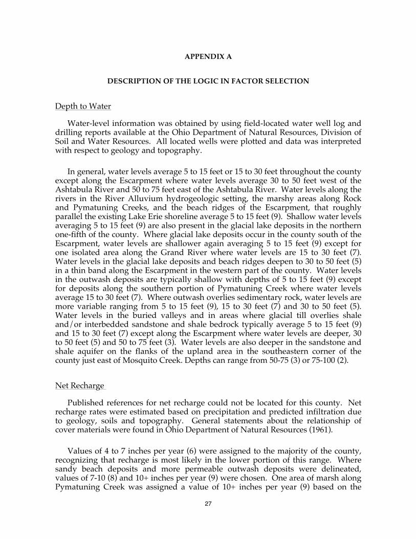
Water-level information was obtained by using field-located water well log and drilling reports available at the Ohio Department of Natural Resources, Division of Soil and Water Resources. All located wells were plotted and data was interpreted with respect to geology and topography.

In general, water levels average 5 to 15 feet or 15 to 30 feet throughout the county except along the Escarpment where water levels average 30 to 50 feet west of the Ashtabula River and 50 to 75 feet east of the Ashtabula River. Water levels along the rivers in the River Alluvium hydrogeologic setting, the marshy areas along Rock and Pymatuning Creeks, and the beach ridges of the Escarpment, that roughly parallel the existing Lake Erie shoreline average 5 to 15 feet (9). Shallow water levels averaging 5 to 15 feet (9) are also present in the glacial lake deposits in the northern one-fifth of the county. Where glacial lake deposits occur in the county south of the Escarpment, water levels are shallower again averaging 5 to 15 feet (9) except for one isolated area along the Grand River where water levels are 15 to 30 feet (7). Water levels in the glacial lake deposits and beach ridges deepen to 30 to 50 feet (5) in a thin band along the Escarpment in the western part of the county. Water levels in the outwash deposits are typically shallow with depths of 5 to 15 feet (9) except for deposits along the southern portion of Pymatuning Creek where water levels average 15 to 30 feet (7). Where outwash overlies sedimentary rock, water levels are more variable ranging from 5 to 15 feet (9), 15 to 30 feet (7) and 30 to 50 feet (5). Water levels in the buried valleys and in areas where glacial till overlies shale and/or interbedded sandstone and shale bedrock typically average 5 to 15 feet (9) and 15 to 30 feet (7) except along the Escarpment where water levels are deeper, 30 to 50 feet (5) and 50 to 75 feet (3). Water levels are also deeper in the sandstone and shale aquifer on the flanks of the upland area in the southeastern corner of the county just east of Mosquito Creek. Depths can range from 50-75 (3) or 75-100 (2).

Net Recharge

Published references for net recharge could not be located for this county. Net recharge rates were estimated based on precipitation and predicted infiltration due to geology, soils and topography. General statements about the relationship of cover materials were found in Ohio Department of Natural Resources (1961).

Values of 4 to 7 inches per year (6) were assigned to the majority of the county, recognizing that recharge is most likely in the lower portion of this range. Where sandy beach deposits and more permeable outwash deposits were delineated, values of 7-10 (8) and 10+ inches per year (9) were chosen. One area of marsh along Pymatuning Creek was assigned a value of 10+ inches per year (9) based on the

28

gravelly surficial deposits. River alluvium and the other marsh area with more clayey surficial deposits were assigned values of 7 to 10 ten inches per year (8). Values of 4 to 7 inches per year (6), 7 to 10 inches per year (8) and 10+ inches per year (9) were chosen in the buried valley based on the character of the overlying surficial deposits.

Aquifer Media

Information on aquifer media was primarily derived from: White and Totten (1979), Hartzell (1978), Risser (1985), Rau (1969), and water well log and drilling reports from the Ohio Department of Natural Resources, Division of Soil and Water Resources. Additional information was gleaned from the Ohio Drilling Company (1971), Cummins (1959), Ohio Department of Natural Resources (1961), Szmuc (1953), Hutton (1940), Bownocker (1965), Goldthwait et al. (1967) and Forsyth (1959).

Sand and gravel deposits within the glacial till were chosen as the aquifer in most areas of the Glacial Lake Deposits hydrogeologic setting and assigned a typical value of (5). Ground water frequently occurs in the glacial till zone between the till/bedrock interface. Where the unconsolidated deposits were thinner than 25 feet (primarily in the western part of the county), the underlying shale was considered the aquifer and assigned a value of (2). In other parts of the county where glacial deposits overlie shale bedrock, the underlying shale was also assigned a value of (2). In the southern part of the county where the till overlies predominantly interbedded sandstone and shale bedrock, the underlying sandstone was chosen as the aquifer and assigned a value of (6). The aquifer in the beach ridges was identified as sand and gravel and assigned a value of (8). Although the beach ridges are of limited thickness, as described by White (1982) in Lake County, they serve as an important source of ground water. Sand and gravel was also chosen as the aquifer in the outwash areas and assigned a value of (8). In the marsh areas, the alluvium along the major rivers, and the alluvium in the northern one-fifth of the county north of the Escarpment areas, sand and gravel was chosen as the aquifer and assigned a typical value of (8). In areas south of the Escarpment where alluvium occurs along tributaries, the underlying bedrock was chosen as the aquifer. In these areas, interbedded sandstone and shale sequences were assigned a value of (6) and shale a value of (2). Sand and gravel was chosen as the aquifer in the Buried Valley hydrogeologic setting. Values of (8) were assigned for the majority of these areas. Where kame deposits were indicated, a value of (9) was assigned because of the abundance of coarse-grained material. Similarly, a value of (7) was assigned in the deltaic deposits to represent the finer fraction.

Soil

Soils were mapped based on the Soil Survey of Ashtabula County (Reeder and Riemenschneider, 1973). The soil media was assigned using the general soil association map in approximately 80 percent of the county; the remainder was re-mapped using DRASTIC-based parameters.

29

Soils formed in the glacial till and glacial lake areas are predominantly silty loam (4). Silty loam is also present in parts of the outwash areas along the southern part of the Grand River and along Rock and Conneaut Creeks and in the tributaries to these and the other rivers and creeks in the county. Sand (9) or gravel (10) predominate in the beach ridges, the alluvium of the major rivers, the outwash areas and the marsh along Pymatuning Creek, but may also be found in other more isolated areas. Shrinking clay (7) is present in a major portion of the Buried Valley hydrogeologic setting coincident with the Grand River northeastward along Coffee Creek and along the southern section of Rock Creek, but also occurs in all other areas of the county except in the areas where glacial deposits overlie bedded sedimentary rock.

Topography

Percent slope was estimated by using 7 1/2 minute USGS topographic quadrangle maps. Contour intervals on the topographic maps were 10 feet on all quadrangles. Topography averages 0 to 2 percent (10) in the majority of the county. Slopes of 2 to 6 percent (9) are encountered only along the Escarpment and adjacent to major rivers.

Impact of the Vadose Zone Media

Information on the vadose zone media was primarily obtained from White and Totten (1979), Risser (1985) and water well log and drilling reports from the Ohio Department of Natural Resources, Division of Soil and Water Resources. Additional information was gleamed from Rau (1969), Hartzell (1978), Szmuc (1953), Bownocker (1965), Goldthwait et al. (1967) and Forsyth (1959).

Silt/clay was chosen as the vadose zone media in all of the Glacial Lake Deposits (7F). The silt/clay designation was assigned a value of (5) in the northern one-third of the county where the surficial deposits are designated Ashtabula Till. Deposits designated as Lavery Till in the southeastern part of the county were also assigned a silt/clay value of (5). A value of (4) was assigned in the majority of the county where the less coarse Hiram Till is the surficial deposit. Till was chosen as the vadose zone media in some areas of the Buried Valley, Glacial Till Over Bedded Sedimentary Rocks, and Glacial Till Over Shale hydrogeologic settings and assigned a value of (4) or (5) based on the presence or absence of sandy clays. Till with a value of (6) was assigned to areas of the Glacial Till Over Shale and Glacial Till Over Bedded Sedimentary Rocks settings where gravelly moraines were present in sufficiently large areas. Where glacial till is thin and/or water levels deeper in the Glacial Till Over Bedded Sedimentary Rocks setting, interbedded sandstone and shale sequences were chosen as the vadose zone media and assigned a typical value of (5). Vadose zone media in the beach ridges was chosen as sand and gravel and assigned a typical value of (8). Sand and gravel was also chosen as the vadose zone media in the outwash areas and assigned a value of (8). The sand and gravel vadose zone in the Buried Valley hydrogeologic setting was assigned values of (9) in kame areas, (8) in terrace areas and (7) in deltaic deposits. Sand and gravel with significant silt and clay was chosen as the vadose zone media in the River Alluvium

30

hydrogeologic setting and the portion of the Buried Valley hydrogeologic setting overlain by alluvial deposits. Values of (6) were assigned along the major rivers and creeks and values of (5) were assigned in the tributaries.

Hydraulic Conductivity of the Aquifer

Only limited published data on hydraulic conductivity of the sandstone bedrock were found for this county in Rau (1969). Values of hydraulic conductivity were primarily estimated by reading descriptions in Hartzell (1978), Ohio Department of Natural Resources (1961), Ohio Drilling Company (1971) and Moody and Associates (1972) and (1973), and referring to the appropriate values referenced by Freeze and Cherry (1979).

Values of 1 to 100 gallons per day per square foot (1) were assigned to the sand and gravel lenses within the glacial till and the shale bedrock based on cited low yields from these areas. Values of 100 to 300 gallons per day per square foot (2) were chosen for the bedded sandstone/shale areas based on information on Rau (1969) and anticipated yields in Hartzell (1978). Values of 300 to 700 gallons per day per square foot (4) were assigned to the sand and gravel aquifer in the buried valley based on anticipated yields in Hartzell (1978). River alluvium, marsh areas and beach ridges were estimated to have values of 700 to 1000 gallons per day per square foot (6). Outwash areas where kames are present were assigned values of 1000 to 2000 gallons per day per square foot (8). A value of 700 to 1000 gallons per day per square foot (6) was assigned to outwash in the terrace areas. Other sand and gravel areas in the buried valley were assigned 700 to 1000 gallons per day per square foot (6) when the aquifer was in the alluvial deposits.

31

APPENDIX B

DESCRIPTION OF HYDROGEOLOGIC SETTINGS AND CHARTS

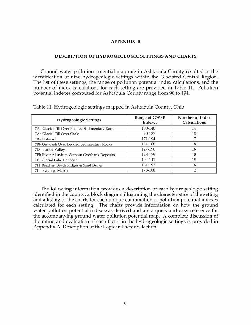
Ground water pollution potential mapping in Ashtabula County resulted in the identification of nine hydrogeologic settings within the Glaciated Central Region. The list of these settings, the range of pollution potential index calculations, and the number of index calculations for each setting are provided in Table 11. Pollution potential indexes computed for Ashtabula County range from 90 to 194.

Table  11.  Hydrogeologic  settings  mapped  in  Ashtabula  County,  Ohio  

Hydrogeologic Settings Range of GWPP Indexes

Number of Index Calculations

7Aa Glacial Till Over Bedded Sedimentary Rocks 100-140 14 7Ae Glacial Till Over Shale 90-137 18 7Ba Outwash 171-194 7 7Bb Outwash Over Bedded Sedimentary Rocks 151-188 8 7D Buried Valley 127-190 16 7Eb River Alluvium Without Overbank Deposits 128-179 10 7F Glacial Lake Deposits 104-141 15 7H Beaches, Beach Ridges & Sand Dunes 161-193 6 7I Swamp/Marsh 178-188 2

The following information provides a description of each hydrogeologic setting identified in the county, a block diagram illustrating the characteristics of the setting and a listing of the charts for each unique combination of pollution potential indexes calculated for each setting. The charts provide information on how the ground water pollution potential index was derived and are a quick and easy reference for the accompanying ground water pollution potential map. A complete discussion of the rating and evaluation of each factor in the hydrogeologic settings is provided in Appendix A, Description of the Logic in Factor Selection.

32

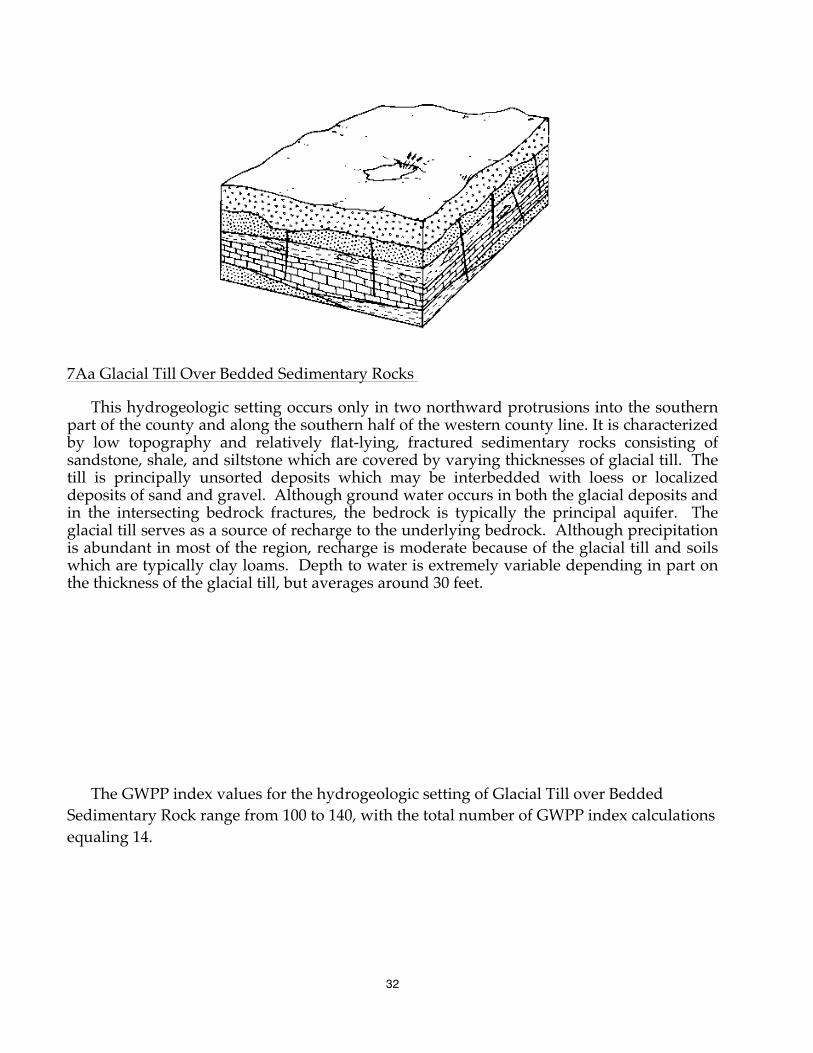
7Aa Glacial Till Over Bedded Sedimentary Rocks

This hydrogeologic setting occurs only in two northward protrusions into the southern part of the county and along the southern half of the western county line. It is characterized by low topography and relatively flat-lying, fractured sedimentary rocks consisting of sandstone, shale, and siltstone which are covered by varying thicknesses of glacial till. The till is principally unsorted deposits which may be interbedded with loess or localized deposits of sand and gravel. Although ground water occurs in both the glacial deposits and in the intersecting bedrock fractures, the bedrock is typically the principal aquifer. The glacial till serves as a source of recharge to the underlying bedrock. Although precipitation is abundant in most of the region, recharge is moderate because of the glacial till and soils which are typically clay loams. Depth to water is extremely variable depending in part on the thickness of the glacial till, but averages around 30 feet.

The  GWPP  index  values  for  the  hydrogeologic  setting  of  Glacial  Till  over  Bedded  Sedimentary  Rock  range  from  100  to  140,  with  the  total  number  of  GWPP  index  calculations  equaling  14.  

33

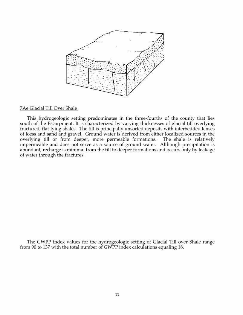
7Ae Glacial Till Over Shale

This hydrogeologic setting predominates in the three-fourths of the county that lies south of the Escarpment. It is characterized by varying thicknesses of glacial till overlying fractured, flat-lying shales. The till is principally unsorted deposits with interbedded lenses of loess and sand and gravel. Ground water is derived from either localized sources in the overlying till or from deeper, more permeable formations. The shale is relatively impermeable and does not serve as a source of ground water. Although precipitation is abundant, recharge is minimal from the till to deeper formations and occurs only by leakage of water through the fractures.

The GWPP index values for the hydrogeologic setting of Glacial Till over Shale range from 90 to 137 with the total number of GWPP index calculations equaling 18.

34

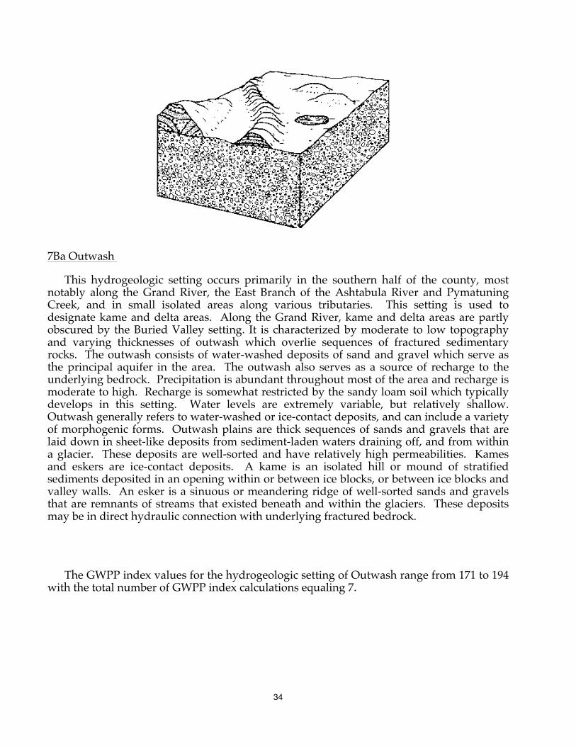
7Ba Outwash

This hydrogeologic setting occurs primarily in the southern half of the county, most notably along the Grand River, the East Branch of the Ashtabula River and Pymatuning Creek, and in small isolated areas along various tributaries. This setting is used to designate kame and delta areas. Along the Grand River, kame and delta areas are partly obscured by the Buried Valley setting. It is characterized by moderate to low topography and varying thicknesses of outwash which overlie sequences of fractured sedimentary rocks. The outwash consists of water-washed deposits of sand and gravel which serve as the principal aquifer in the area. The outwash also serves as a source of recharge to the underlying bedrock. Precipitation is abundant throughout most of the area and recharge is moderate to high. Recharge is somewhat restricted by the sandy loam soil which typically develops in this setting. Water levels are extremely variable, but relatively shallow. Outwash generally refers to water-washed or ice-contact deposits, and can include a variety of morphogenic forms. Outwash plains are thick sequences of sands and gravels that are laid down in sheet-like deposits from sediment-laden waters draining off, and from within a glacier. These deposits are well-sorted and have relatively high permeabilities. Kames and eskers are ice-contact deposits. A kame is an isolated hill or mound of stratified sediments deposited in an opening within or between ice blocks, or between ice blocks and valley walls. An esker is a sinuous or meandering ridge of well-sorted sands and gravels that are remnants of streams that existed beneath and within the glaciers. These deposits may be in direct hydraulic connection with underlying fractured bedrock.

The GWPP index values for the hydrogeologic setting of Outwash range from 171 to 194 with the total number of GWPP index calculations equaling 7.

35

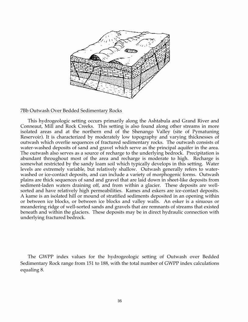
7Bb Outwash Over Bedded Sedimentary Rocks

This hydrogeologic setting occurs primarily along the Ashtabula and Grand River and Conneaut, Mill and Rock Creeks. This setting is also found along other streams in more isolated areas and at the northern end of the Shenango Valley (site of Pymatuning Reservoir). It is characterized by moderately low topography and varying thicknesses of outwash which overlie sequences of fractured sedimentary rocks. The outwash consists of water-washed deposits of sand and gravel which serve as the principal aquifer in the area. The outwash also serves as a source of recharge to the underlying bedrock. Precipitation is abundant throughout most of the area and recharge is moderate to high. Recharge is somewhat restricted by the sandy loam soil which typically develops in this setting. Water levels are extremely variable, but relatively shallow. Outwash generally refers to water-washed or ice-contact deposits, and can include a variety of morphogenic forms. Outwash plains are thick sequences of sand and gravel that are laid down in sheet-like deposits from sediment-laden waters draining off, and from within a glacier. These deposits are well-sorted and have relatively high permeabilities. Kames and eskers are ice-contact deposits. A kame is an isolated hill or mound of stratified sediments deposited in an opening within or between ice blocks, or between ice blocks and valley walls. An esker is a sinuous or meandering ridge of well-sorted sands and gravels that are remnants of streams that existed beneath and within the glaciers. These deposits may be in direct hydraulic connection with underlying fractured bedrock.

The   GWPP   index   values   for   the   hydrogeologic   setting   of   Outwash   over   Bedded  Sedimentary  Rock  range  from  151  to  188,  with  the  total  number  of  GWPP  index  calculations  equaling  8.  

36

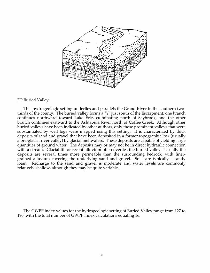
7D Buried Valley

This hydrogeologic setting underlies and parallels the Grand River in the southern two-thirds of the county. The buried valley forms a "Y" just south of the Escarpment; one branch continues northward toward Lake Erie, culminating north of Saybrook, and the other branch continues eastward to the Ashtabula River north of Coffee Creek. Although other buried valleys have been indicated by other authors, only those prominent valleys that were substantiated by well logs were mapped using this setting. It is characterized by thick deposits of sand and gravel that have been deposited in a former topographic low (usually a pre-glacial river valley) by glacial meltwaters. These deposits are capable of yielding large quantities of ground water. The deposits may or may not be in direct hydraulic connection with a stream. Glacial till or recent alluvium often overlies the buried valley. Usually the deposits are several times more permeable than the surrounding bedrock, with finer-grained alluvium covering the underlying sand and gravel. Soils are typically a sandy loam. Recharge to the sand and gravel is moderate and water levels are commonly relatively shallow, although they may be quite variable.

The GWPP index values for the hydrogeologic setting of Buried Valley range from 127 to 190, with the total number of GWPP index calculations equaling 16.

37

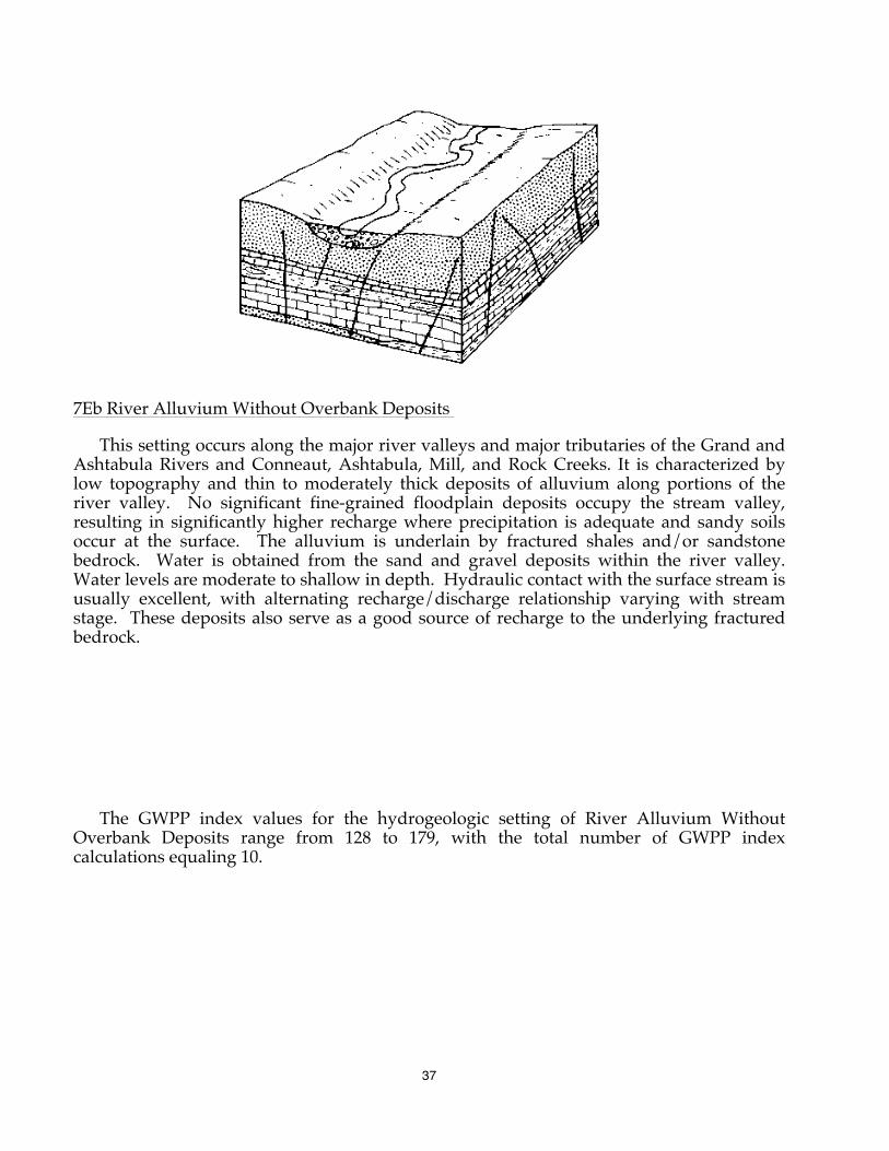
7Eb River Alluvium Without Overbank Deposits

This setting occurs along the major river valleys and major tributaries of the Grand and Ashtabula Rivers and Conneaut, Ashtabula, Mill, and Rock Creeks. It is characterized by low topography and thin to moderately thick deposits of alluvium along portions of the river valley. No significant fine-grained floodplain deposits occupy the stream valley, resulting in significantly higher recharge where precipitation is adequate and sandy soils occur at the surface. The alluvium is underlain by fractured shales and/or sandstone bedrock. Water is obtained from the sand and gravel deposits within the river valley. Water levels are moderate to shallow in depth. Hydraulic contact with the surface stream is usually excellent, with alternating recharge/discharge relationship varying with stream stage. These deposits also serve as a good source of recharge to the underlying fractured bedrock.

The GWPP index values for the hydrogeologic setting of River Alluvium Without Overbank Deposits range from 128 to 179, with the total number of GWPP index calculations equaling 10.

38

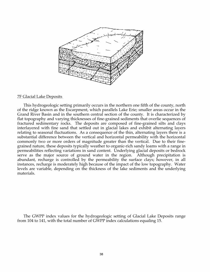
7F Glacial Lake Deposits

This hydrogeologic setting primarily occurs in the northern one fifth of the county, north of the ridge known as the Escarpment, which parallels Lake Erie; smaller areas occur in the Grand River Basin and in the southern central section of the county. It is characterized by flat topography and varying thicknesses of fine-grained sediments that overlie sequences of fractured sedimentary rocks. The deposits are composed of fine-grained silts and clays interlayered with fine sand that settled out in glacial lakes and exhibit alternating layers relating to seasonal fluctuations. As a consequence of the thin, alternating layers there is a substantial difference between the vertical and horizontal permeability with the horizontal commonly two or more orders of magnitude greater than the vertical. Due to their fine-grained nature, these deposits typically weather to organic-rich sandy loams with a range in permeabilities reflecting variations in sand content. Underlying glacial deposits or bedrock serve as the major source of ground water in the region. Although precipitation is abundant, recharge is controlled by the permeability the surface clays; however, in all instances, recharge is moderately high because of the impact of the low topography. Water levels are variable, depending on the thickness of the lake sediments and the underlying materials.

The GWPP index values for the hydrogeologic setting of Glacial Lake Deposits range from 104 to 141, with the total number of GWPP index calculations equaling 15.

39

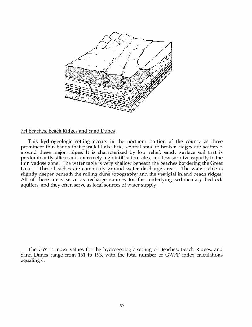
7H Beaches, Beach Ridges and Sand Dunes

This hydrogeologic setting occurs in the northern portion of the county as three prominent thin bands that parallel Lake Erie; several smaller broken ridges are scattered around these major ridges. It is characterized by low relief, sandy surface soil that is predominantly silica sand, extremely high infiltration rates, and low sorptive capacity in the thin vadose zone. The water table is very shallow beneath the beaches bordering the Great Lakes. These beaches are commonly ground water discharge areas. The water table is slightly deeper beneath the rolling dune topography and the vestigial inland beach ridges. All of these areas serve as recharge sources for the underlying sedimentary bedrock aquifers, and they often serve as local sources of water supply.

The GWPP index values for the hydrogeologic setting of Beaches, Beach Ridges, and Sand Dunes range from 161 to 193, with the total number of GWPP index calculations equaling 6.

40

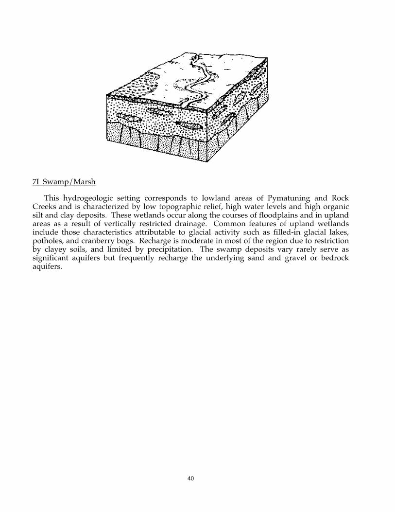
7I Swamp/Marsh

This hydrogeologic setting corresponds to lowland areas of Pymatuning and Rock Creeks and is characterized by low topographic relief, high water levels and high organic silt and clay deposits. These wetlands occur along the courses of floodplains and in upland areas as a result of vertically restricted drainage. Common features of upland wetlands include those characteristics attributable to glacial activity such as filled-in glacial lakes, potholes, and cranberry bogs. Recharge is moderate in most of the region due to restriction by clayey soils, and limited by precipitation. The swamp deposits vary rarely serve as significant aquifers but frequently recharge the underlying sand and gravel or bedrock aquifers.

41

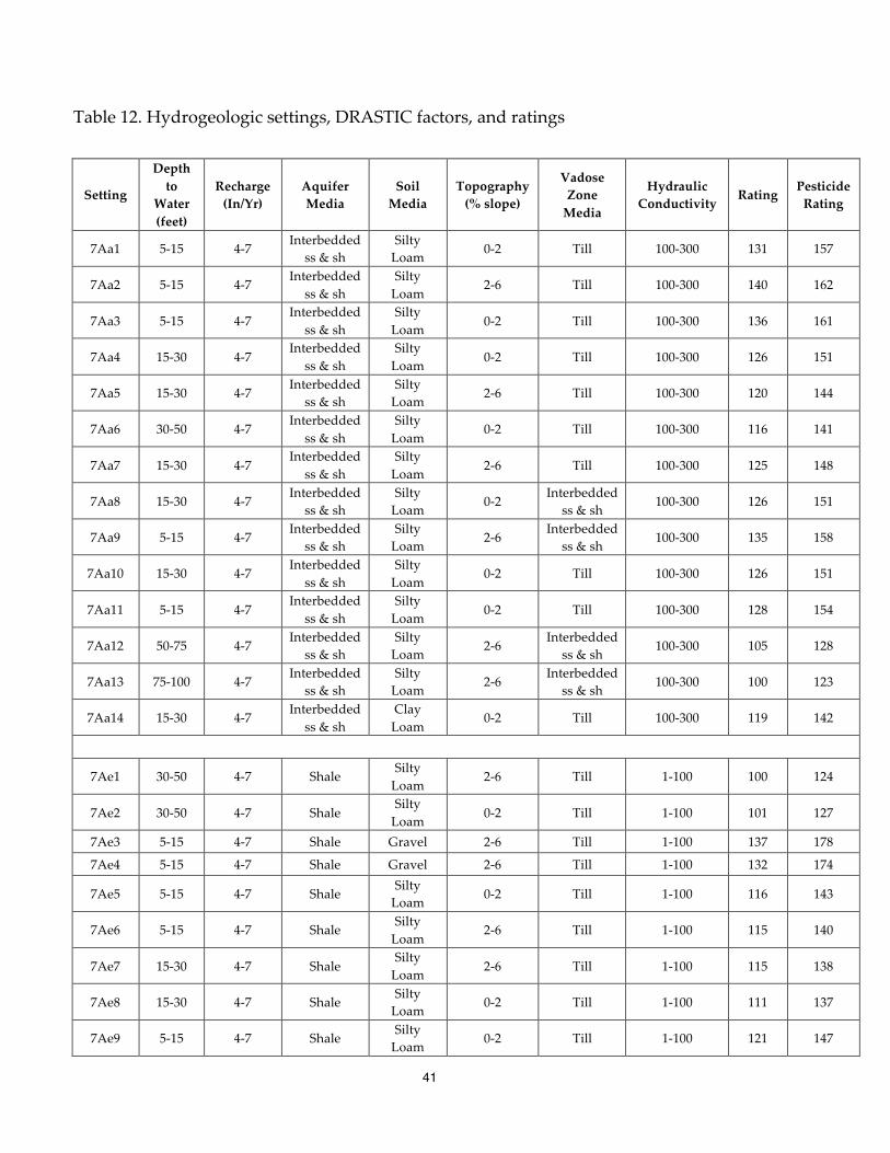
Table  12.  Hydrogeologic  settings,  DRASTIC  factors,  and  ratings  

Setting  

Depth  to  

Water  (feet)  

Recharge  (In/Yr)  

Aquifer  Media  

Soil  Media  

Topography  (%  slope)  

Vadose  Zone  Media  

Hydraulic  Conductivity  

Rating  Pesticide  Rating  

7Aa1   5-­‐‑15   4-­‐‑7  Interbedded  

ss  &  sh  Silty  Loam  

0-­‐‑2   Till   100-­‐‑300   131   157  

7Aa2   5-­‐‑15   4-­‐‑7  Interbedded  

ss  &  sh  Silty  Loam  

2-­‐‑6   Till   100-­‐‑300   140   162  

7Aa3   5-­‐‑15   4-­‐‑7  Interbedded  

ss  &  sh  Silty  Loam  

0-­‐‑2   Till   100-­‐‑300   136   161  

7Aa4   15-­‐‑30   4-­‐‑7  Interbedded  

ss  &  sh  Silty  Loam  

0-­‐‑2   Till   100-­‐‑300   126   151  

7Aa5   15-­‐‑30   4-­‐‑7  Interbedded  

ss  &  sh  Silty  Loam  

2-­‐‑6   Till   100-­‐‑300   120   144  

7Aa6   30-­‐‑50   4-­‐‑7  Interbedded  

ss  &  sh  Silty  Loam  

0-­‐‑2   Till   100-­‐‑300   116   141  

7Aa7   15-­‐‑30   4-­‐‑7  Interbedded  

ss  &  sh  Silty  Loam  

2-­‐‑6   Till   100-­‐‑300   125   148  

7Aa8   15-­‐‑30   4-­‐‑7  Interbedded  

ss  &  sh  Silty  Loam  

0-­‐‑2  Interbedded  

ss  &  sh  100-­‐‑300   126   151  

7Aa9   5-­‐‑15   4-­‐‑7  Interbedded  

ss  &  sh  Silty  Loam  

2-­‐‑6  Interbedded  

ss  &  sh  100-­‐‑300   135   158  

7Aa10   15-­‐‑30   4-­‐‑7  Interbedded  

ss  &  sh  Silty  Loam  

0-­‐‑2   Till   100-­‐‑300   126   151  

7Aa11   5-­‐‑15   4-­‐‑7  Interbedded  

ss  &  sh  Silty  Loam  

0-­‐‑2   Till   100-­‐‑300   128   154  

7Aa12   50-­‐‑75   4-­‐‑7  Interbedded  

ss  &  sh  Silty  Loam  

2-­‐‑6  Interbedded  

ss  &  sh  100-­‐‑300   105   128  

7Aa13   75-­‐‑100   4-­‐‑7  Interbedded  

ss  &  sh  Silty  Loam  

2-­‐‑6  Interbedded  

ss  &  sh  100-­‐‑300   100   123  

7Aa14   15-­‐‑30   4-­‐‑7  Interbedded  

ss  &  sh  Clay  Loam  

0-­‐‑2   Till   100-­‐‑300   119   142  

 

7Ae1   30-­‐‑50   4-­‐‑7   Shale  Silty  Loam  

2-­‐‑6   Till   1-­‐‑100   100   124  

7Ae2   30-­‐‑50   4-­‐‑7   Shale  Silty  Loam  

0-­‐‑2   Till   1-­‐‑100   101   127  

7Ae3   5-­‐‑15   4-­‐‑7   Shale   Gravel   2-­‐‑6   Till   1-­‐‑100   137   178  

7Ae4   5-­‐‑15   4-­‐‑7   Shale   Gravel   2-­‐‑6   Till   1-­‐‑100   132   174  

7Ae5   5-­‐‑15   4-­‐‑7   Shale  Silty  Loam  

0-­‐‑2   Till   1-­‐‑100   116   143  

7Ae6   5-­‐‑15   4-­‐‑7   Shale  Silty  Loam  

2-­‐‑6   Till   1-­‐‑100   115   140  

7Ae7   15-­‐‑30   4-­‐‑7   Shale  Silty  Loam  

2-­‐‑6   Till   1-­‐‑100   115   138  

7Ae8   15-­‐‑30   4-­‐‑7   Shale  Silty  Loam  

0-­‐‑2   Till   1-­‐‑100   111   137  

7Ae9   5-­‐‑15   4-­‐‑7   Shale  Silty  Loam  

0-­‐‑2   Till   1-­‐‑100   121   147  

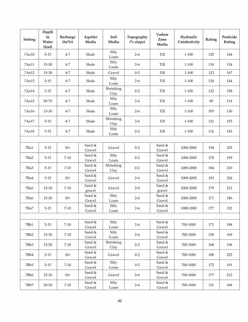
42

Setting  

Depth  to  

Water  (feet)  

Recharge  (In/Yr)  

Aquifer  Media  

Soil  Media  

Topography  (%  slope)  

Vadose  Zone  Media  

Hydraulic  Conductivity  

Rating  Pesticide  Rating  

7Ae10   5-­‐‑15   4-­‐‑7   Shale  Silty  Loam  

2-­‐‑6   Till   1-­‐‑100   120   144  

7Ae11   15-­‐‑30   4-­‐‑7   Shale  Silty  Loam  

2-­‐‑6   Till   1-­‐‑100   110   134  

7Ae12   15-­‐‑30   4-­‐‑7   Shale   Gravel   0-­‐‑2   Till   1-­‐‑100   123   167  

7Ae13   5-­‐‑15   4-­‐‑7   Shale  Silty  Loam  

2-­‐‑6   Till   1-­‐‑100   120   144  

7Ae14   5-­‐‑15   4-­‐‑7   Shale  Shrinking  

Clay  0-­‐‑2   Till   1-­‐‑100   122   158  

7Ae15   50-­‐‑75   4-­‐‑7   Shale  Silty  Loam  

2-­‐‑6   Till   1-­‐‑100   90   114  

7Ae16   15-­‐‑30   4-­‐‑7   Shale  Silty  Loam  

2-­‐‑6   Till   1-­‐‑100   105   130  

7Ae17   5-­‐‑15   4-­‐‑7   Shale  Shrinking  

Clay  2-­‐‑6   Till   1-­‐‑100   121   155  

7Ae18   5-­‐‑15   4-­‐‑7   Shale  Silty  Loam  

0-­‐‑2   Till   1-­‐‑100   116   143  

 

7Ba1   5-­‐‑15   10+  Sand  &  Gravel  

Gravel   0-­‐‑2  Sand  &  Gravel  

1000-­‐‑2000   194   229  

7Ba2   5-­‐‑15   7-­‐‑10  Sand  &  Gravel  

Silty  Loam  

0-­‐‑2  Sand  &  Gravel  

1000-­‐‑2000   178   195  

7Ba3   5-­‐‑15   7-­‐‑10  Sand  &  Gravel  

Shrinking  Clay  

0-­‐‑2  Sand  &  Gravel  

1000-­‐‑2000   184   210  

7Ba4   5-­‐‑15   10+  Sand  &  Gravel  

Gravel   2-­‐‑6  Sand  &  Gravel  

1000-­‐‑2000   193   226  

7Ba5   15-­‐‑30   7-­‐‑10  Sand  &  gravel  

Gravel   2-­‐‑6  Sand  &  gravel  

1000-­‐‑2000   179   212  

7Ba6   15-­‐‑30   10+  Sand  &  Gravel  

Silty  Loam  

2-­‐‑6  Sand  &  Gravel  

1000-­‐‑2000   171   186  

7Ba7   5-­‐‑15   7-­‐‑10  Sand  &  Gravel  

Silty  Loam  

2-­‐‑6  Sand  &  Gravel  

1000-­‐‑2000   177   192  

 

7Bb1   5-­‐‑15   7-­‐‑10  Sand  &  Gravel  

Silty  Loam  

2-­‐‑6  Sand  &  Gravel  

700-­‐‑1000   171   188  

7Bb2   15-­‐‑30   7-­‐‑10  Sand  &  Gravel  

Silty  Loam  

2-­‐‑6  Sand  &  Gravel  

700-­‐‑1000   158   169  

7Bb3   15-­‐‑30   7-­‐‑10  Sand  &  Gravel  

Shrinking  Clay  

0-­‐‑2  Sand  &  Gravel  

700-­‐‑1000   168   196  

7Bb4   5-­‐‑15   10+  Sand  &  Gravel  

Gravel   0-­‐‑2  Sand  &  Gravel  

700-­‐‑1000   188   225  

7Bb5   5-­‐‑15   7-­‐‑10  Sand  &  Gravel  

Silty  Loam  

0-­‐‑2  Sand  &  Gravel  

700-­‐‑1000   172   191  

7Bb6   15-­‐‑30   10+  Sand  &  Gravel  

Gravel   2-­‐‑6  Sand  &  Gravel  

700-­‐‑1000   177   212  

7Bb7   30-­‐‑50   7-­‐‑10  Sand  &  Gravel  

Silty  Loam  

2-­‐‑6  Sand  &  Gravel  

700-­‐‑1000   151   168  

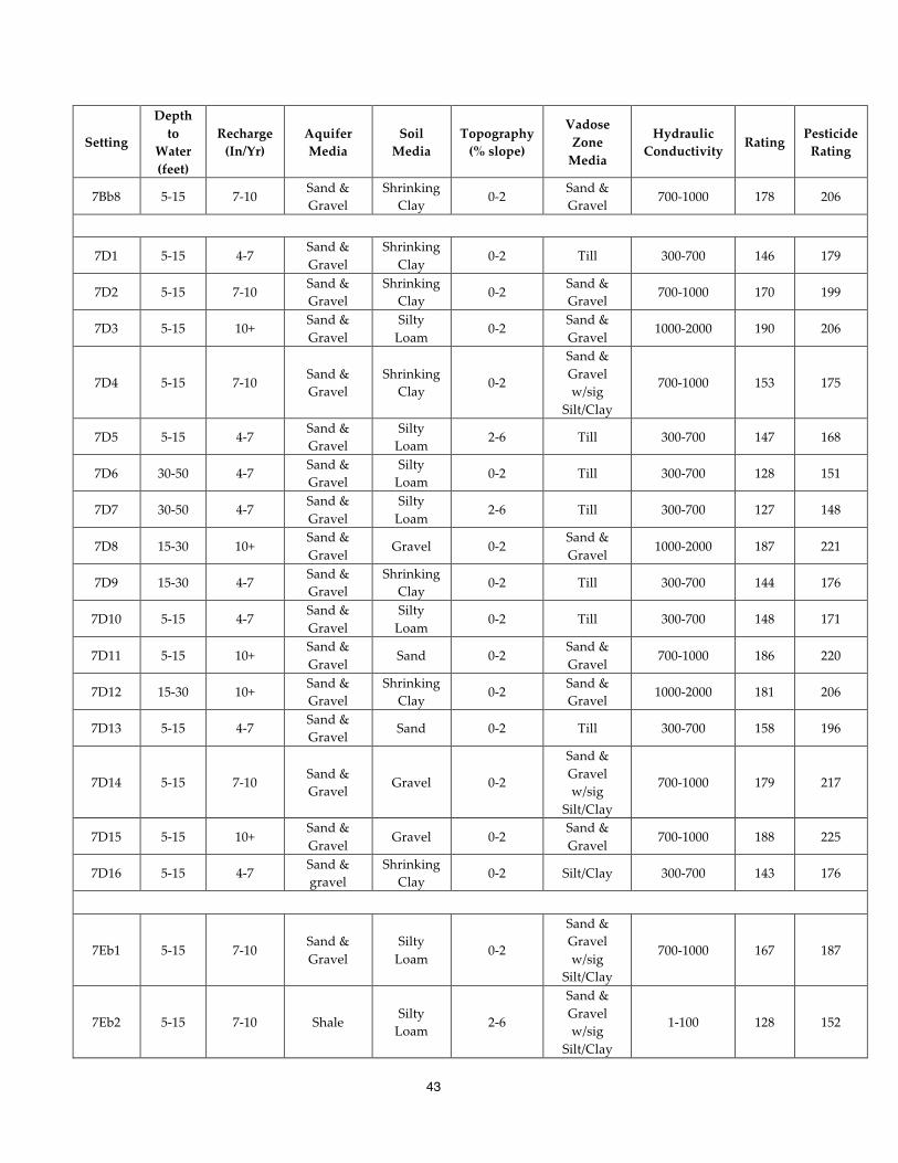
43

Setting  

Depth  to  

Water  (feet)  

Recharge  (In/Yr)  

Aquifer  Media  

Soil  Media  

Topography  (%  slope)  

Vadose  Zone  Media  

Hydraulic  Conductivity  

Rating  Pesticide  Rating  

7Bb8   5-­‐‑15   7-­‐‑10  Sand  &  Gravel  

Shrinking  Clay  

0-­‐‑2  Sand  &  Gravel  

700-­‐‑1000   178   206  

 

7D1   5-­‐‑15   4-­‐‑7  Sand  &  Gravel  

Shrinking  Clay  

0-­‐‑2   Till   300-­‐‑700   146   179  

7D2   5-­‐‑15   7-­‐‑10  Sand  &  Gravel  

Shrinking  Clay  

0-­‐‑2  Sand  &  Gravel  

700-­‐‑1000   170   199  

7D3   5-­‐‑15   10+  Sand  &  Gravel  

Silty  Loam  

0-­‐‑2  Sand  &  Gravel  

1000-­‐‑2000   190   206  

7D4   5-­‐‑15   7-­‐‑10  Sand  &  Gravel  

Shrinking  Clay  

0-­‐‑2  

Sand  &  Gravel  w/sig  

Silt/Clay  

700-­‐‑1000   153   175  

7D5   5-­‐‑15   4-­‐‑7  Sand  &  Gravel  

Silty  Loam  

2-­‐‑6   Till   300-­‐‑700   147   168  

7D6   30-­‐‑50   4-­‐‑7  Sand  &  Gravel  

Silty  Loam  

0-­‐‑2   Till   300-­‐‑700   128   151  

7D7   30-­‐‑50   4-­‐‑7  Sand  &  Gravel  

Silty  Loam  

2-­‐‑6   Till   300-­‐‑700   127   148  

7D8   15-­‐‑30   10+  Sand  &  Gravel  

Gravel   0-­‐‑2  Sand  &  Gravel  

1000-­‐‑2000   187   221  

7D9   15-­‐‑30   4-­‐‑7  Sand  &  Gravel  

Shrinking  Clay  

0-­‐‑2   Till   300-­‐‑700   144   176  

7D10   5-­‐‑15   4-­‐‑7  Sand  &  Gravel  

Silty  Loam  

0-­‐‑2   Till   300-­‐‑700   148   171  

7D11   5-­‐‑15   10+  Sand  &  Gravel  

Sand   0-­‐‑2  Sand  &  Gravel  

700-­‐‑1000   186   220  

7D12   15-­‐‑30   10+  Sand  &  Gravel  

Shrinking  Clay  

0-­‐‑2  Sand  &  Gravel  

1000-­‐‑2000   181   206  

7D13   5-­‐‑15   4-­‐‑7  Sand  &  Gravel  

Sand   0-­‐‑2   Till   300-­‐‑700   158   196  

7D14   5-­‐‑15   7-­‐‑10  Sand  &  Gravel  

Gravel   0-­‐‑2  

Sand  &  Gravel  w/sig  

Silt/Clay  

700-­‐‑1000   179   217  

7D15   5-­‐‑15   10+  Sand  &  Gravel  

Gravel   0-­‐‑2  Sand  &  Gravel  

700-­‐‑1000   188   225  

7D16   5-­‐‑15   4-­‐‑7  Sand  &  gravel  

Shrinking  Clay  

0-­‐‑2   Silt/Clay   300-­‐‑700   143   176  

 

7Eb1   5-­‐‑15   7-­‐‑10  Sand  &  Gravel  

Silty  Loam  

0-­‐‑2  

Sand  &  Gravel  w/sig  

Silt/Clay  

700-­‐‑1000   167   187  

7Eb2   5-­‐‑15   7-­‐‑10   Shale  Silty  Loam  

2-­‐‑6  

Sand  &  Gravel  w/sig  

Silt/Clay  

1-­‐‑100   128   152  

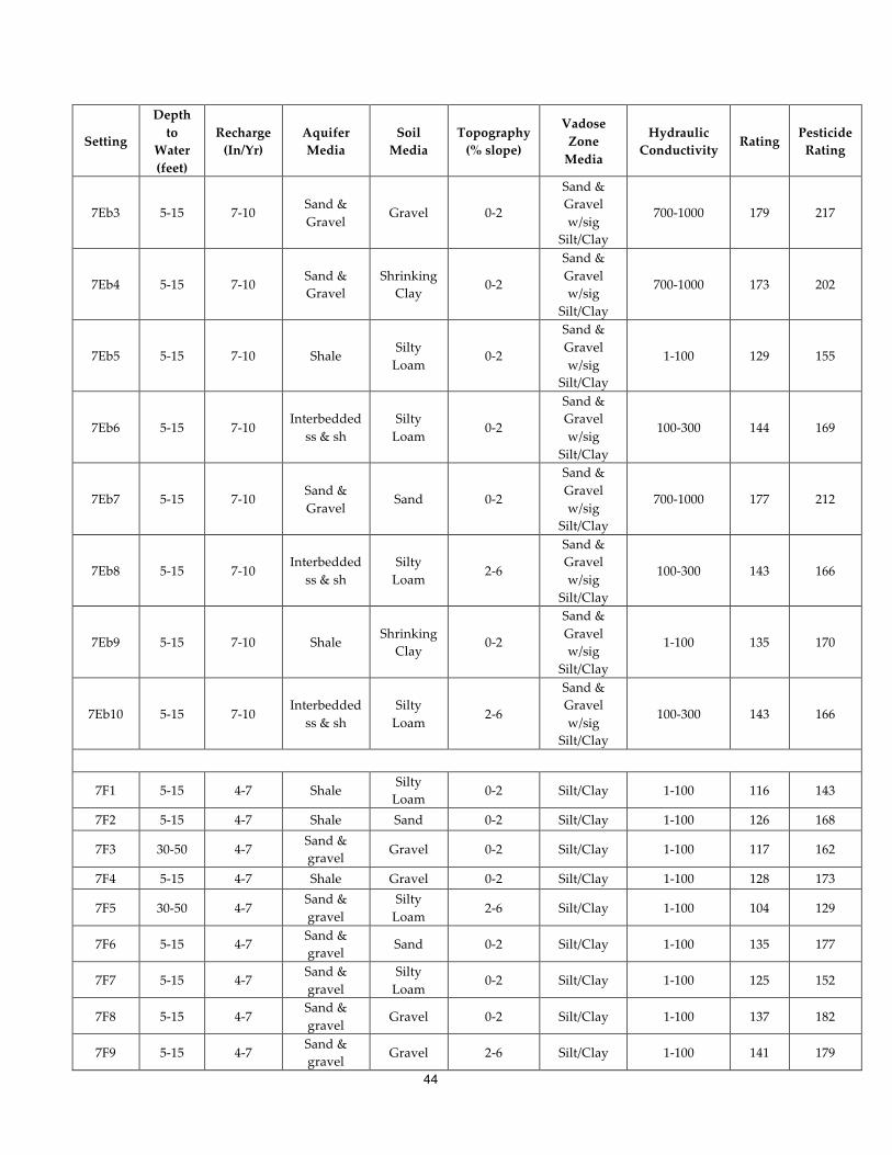
44

Setting  

Depth  to  

Water  (feet)  

Recharge  (In/Yr)  

Aquifer  Media  

Soil  Media  

Topography  (%  slope)  

Vadose  Zone  Media  

Hydraulic  Conductivity  

Rating  Pesticide  Rating  

7Eb3   5-­‐‑15   7-­‐‑10  Sand  &  Gravel  

Gravel   0-­‐‑2  

Sand  &  Gravel  w/sig  

Silt/Clay  

700-­‐‑1000   179   217  

7Eb4   5-­‐‑15   7-­‐‑10  Sand  &  Gravel  

Shrinking  Clay  

0-­‐‑2  

Sand  &  Gravel  w/sig  

Silt/Clay  

700-­‐‑1000   173   202  

7Eb5   5-­‐‑15   7-­‐‑10   Shale  Silty  Loam  

0-­‐‑2  

Sand  &  Gravel  w/sig  

Silt/Clay  

1-­‐‑100   129   155  

7Eb6   5-­‐‑15   7-­‐‑10  Interbedded  

ss  &  sh  Silty  Loam  

0-­‐‑2  

Sand  &  Gravel  w/sig  

Silt/Clay  

100-­‐‑300   144   169  

7Eb7   5-­‐‑15   7-­‐‑10  Sand  &  Gravel  

Sand   0-­‐‑2  

Sand  &  Gravel  w/sig  

Silt/Clay  

700-­‐‑1000   177   212  

7Eb8   5-­‐‑15   7-­‐‑10  Interbedded  

ss  &  sh  Silty  Loam  

2-­‐‑6  

Sand  &  Gravel  w/sig  

Silt/Clay  

100-­‐‑300   143   166  

7Eb9   5-­‐‑15   7-­‐‑10   Shale  Shrinking  

Clay  0-­‐‑2  

Sand  &  Gravel  w/sig  

Silt/Clay  

1-­‐‑100   135   170  

7Eb10   5-­‐‑15   7-­‐‑10  Interbedded  

ss  &  sh  Silty  Loam  

2-­‐‑6  

Sand  &  Gravel  w/sig  

Silt/Clay  

100-­‐‑300   143   166  

 

7F1   5-­‐‑15   4-­‐‑7   Shale  Silty  Loam  

0-­‐‑2   Silt/Clay   1-­‐‑100   116   143  

7F2   5-­‐‑15   4-­‐‑7   Shale   Sand   0-­‐‑2   Silt/Clay   1-­‐‑100   126   168  

7F3   30-­‐‑50   4-­‐‑7  Sand  &  gravel  

Gravel   0-­‐‑2   Silt/Clay   1-­‐‑100   117   162  

7F4   5-­‐‑15   4-­‐‑7   Shale   Gravel   0-­‐‑2   Silt/Clay   1-­‐‑100   128   173  

7F5   30-­‐‑50   4-­‐‑7  Sand  &  gravel  

Silty  Loam  

2-­‐‑6   Silt/Clay   1-­‐‑100   104   129  

7F6   5-­‐‑15   4-­‐‑7  Sand  &  gravel  

Sand   0-­‐‑2   Silt/Clay   1-­‐‑100   135   177  

7F7   5-­‐‑15   4-­‐‑7  Sand  &  gravel  

Silty  Loam  

0-­‐‑2   Silt/Clay   1-­‐‑100   125   152  

7F8   5-­‐‑15   4-­‐‑7  Sand  &  gravel  

Gravel   0-­‐‑2   Silt/Clay   1-­‐‑100   137   182  

7F9   5-­‐‑15   4-­‐‑7  Sand  &  gravel  

Gravel   2-­‐‑6   Silt/Clay   1-­‐‑100   141   179  

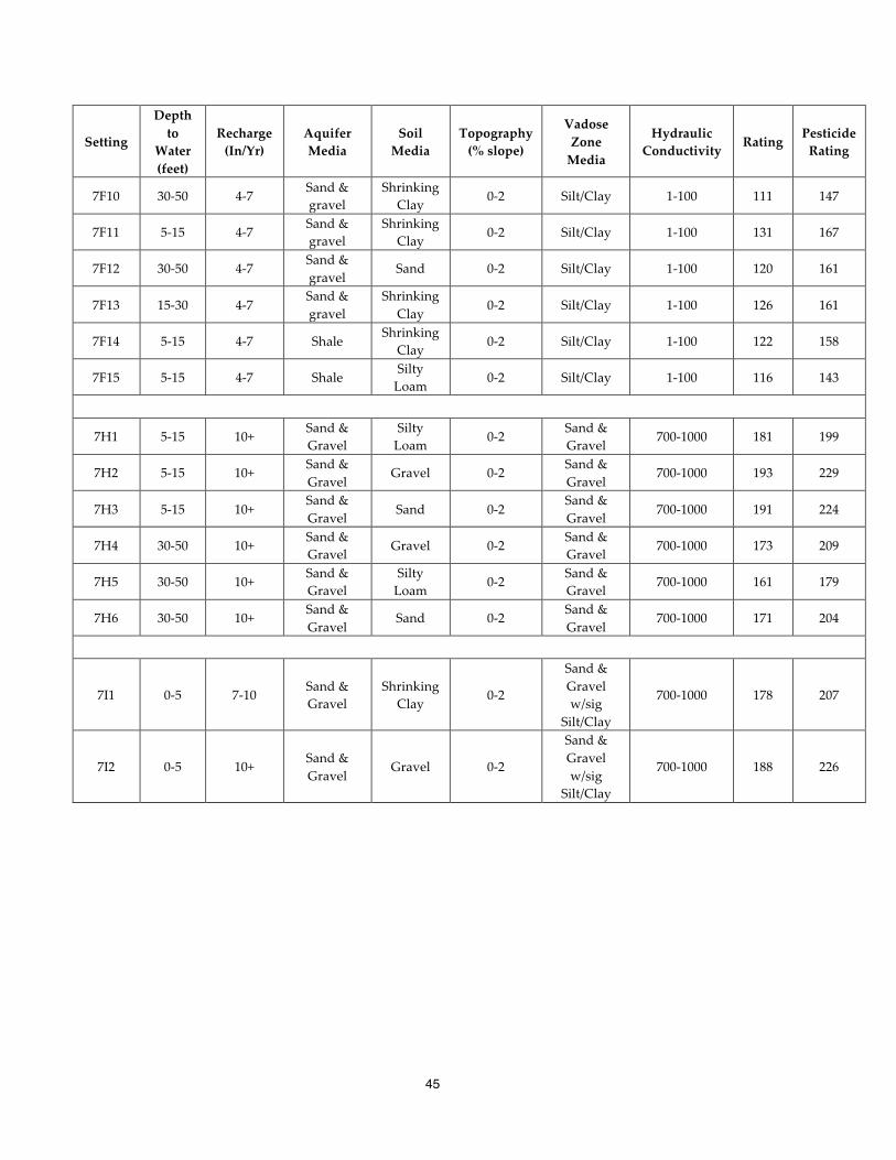
45

Setting  

Depth  to  

Water  (feet)  

Recharge  (In/Yr)  

Aquifer  Media  

Soil  Media  

Topography  (%  slope)  

Vadose  Zone  Media  

Hydraulic  Conductivity  

Rating  Pesticide  Rating  

7F10   30-­‐‑50   4-­‐‑7  Sand  &  gravel  

Shrinking  Clay  

0-­‐‑2   Silt/Clay   1-­‐‑100   111   147  

7F11   5-­‐‑15   4-­‐‑7  Sand  &  gravel  

Shrinking  Clay  

0-­‐‑2   Silt/Clay   1-­‐‑100   131   167  

7F12   30-­‐‑50   4-­‐‑7  Sand  &  gravel  

Sand   0-­‐‑2   Silt/Clay   1-­‐‑100   120   161  

7F13   15-­‐‑30   4-­‐‑7  Sand  &  gravel  

Shrinking  Clay  

0-­‐‑2   Silt/Clay   1-­‐‑100   126   161  

7F14   5-­‐‑15   4-­‐‑7   Shale  Shrinking  

Clay  0-­‐‑2   Silt/Clay   1-­‐‑100   122   158  

7F15   5-­‐‑15   4-­‐‑7   Shale  Silty  Loam  

0-­‐‑2   Silt/Clay   1-­‐‑100   116   143  

 

7H1   5-­‐‑15   10+  Sand  &  Gravel  

Silty  Loam  

0-­‐‑2  Sand  &  Gravel  

700-­‐‑1000   181   199  

7H2   5-­‐‑15   10+  Sand  &  Gravel  

Gravel   0-­‐‑2  Sand  &  Gravel  

700-­‐‑1000   193   229  

7H3   5-­‐‑15   10+  Sand  &  Gravel  

Sand   0-­‐‑2  Sand  &  Gravel  

700-­‐‑1000   191   224  

7H4   30-­‐‑50   10+  Sand  &  Gravel  

Gravel   0-­‐‑2  Sand  &  Gravel  

700-­‐‑1000   173   209  

7H5   30-­‐‑50   10+  Sand  &  Gravel  

Silty  Loam  

0-­‐‑2  Sand  &  Gravel  

700-­‐‑1000   161   179  

7H6   30-­‐‑50   10+  Sand  &  Gravel  

Sand   0-­‐‑2  Sand  &  Gravel  

700-­‐‑1000   171   204  

 

7I1   0-­‐‑5   7-­‐‑10  Sand  &  Gravel  

Shrinking  Clay  

0-­‐‑2  

Sand  &  Gravel  w/sig  

Silt/Clay  

700-­‐‑1000   178   207  

7I2   0-­‐‑5   10+  Sand  &  Gravel  

Gravel   0-­‐‑2  

Sand  &  Gravel  w/sig  

Silt/Clay  

700-­‐‑1000   188   226  

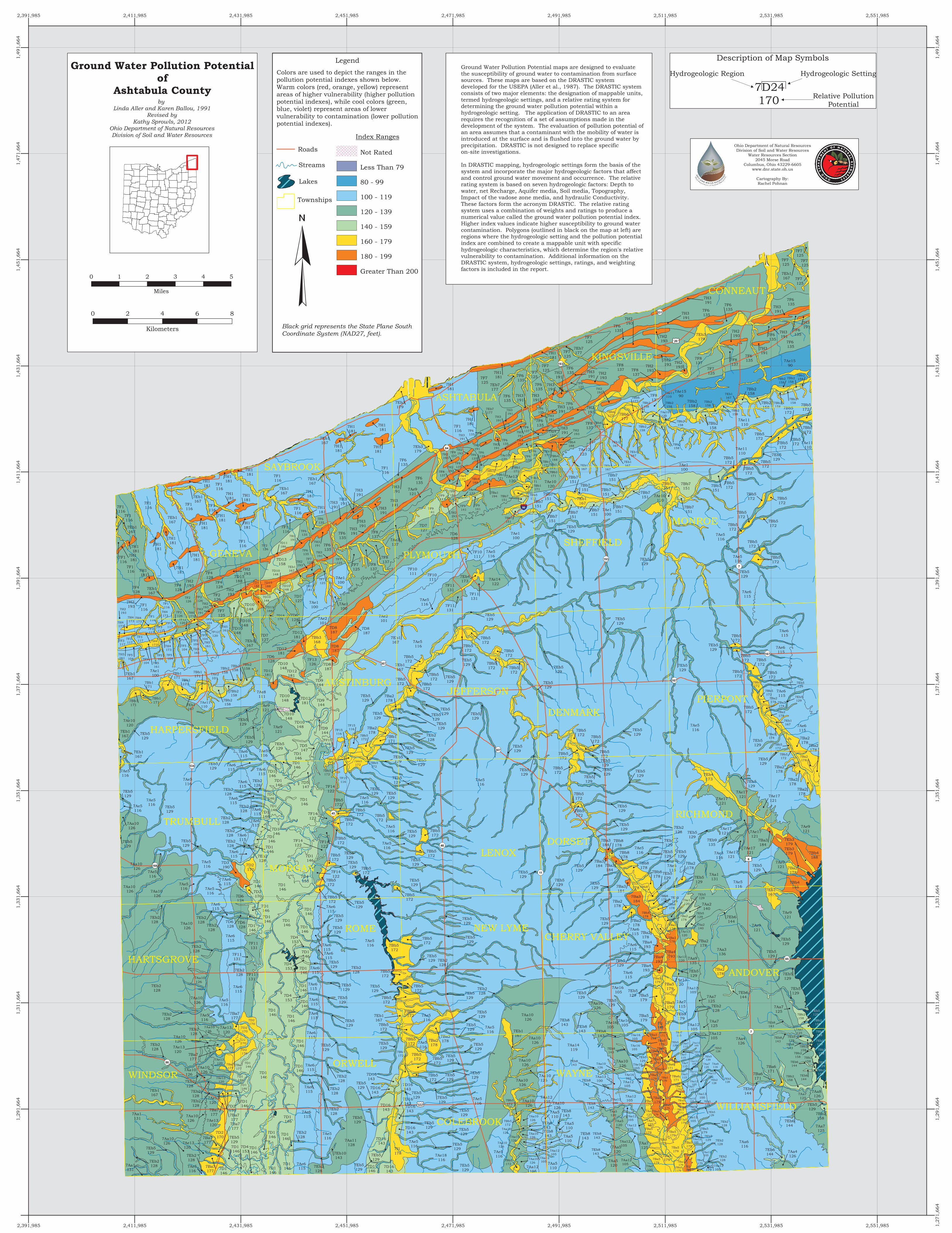
7Ae5 116

7Ae5 116

7Ae5 116

7Ae5 116

7Ae5 116

7Ae5 116

7Eb2 128

7Aa6 116

7Aa4 126

7D4 153

7Aa14 119

7Ae11 110

7F1 116

7F1 116

7F6 135

7Ae5 116

7F8 137

7D1 146

7F1 116

7Aa3 136

7Aa10 126

7F1 116

7Ae1 100

7D6 128

7D1 146

7Aa1 131

7Eb1 167

7D7 127

7F1 116

7Ae10 120

7Ae9 121

7Ae5 116

7Ae15 90

7Aa10 126

7Aa10 126

7I2 188

7F1 116

7Ae1 100

7Ae2 101

7D1 146

7F7 125

7D1 146

7Ae5 116

7F1 116

7Ae9 121

7D7 127

7D1 146

7F6 135

7Ae1 100

7Ae6 115

7D6 128

7F6 135

7Aa1 131

7Ae5 116

7Ae5 116

7Ae2 101

7D1 146

7Aa11 128

7Ae6 115

7Ae16 105

7D10 148

7F10 111

7Aa10 126

7Ae6 115

7Ae6 115

7F6 135

7F2 126

7Ae11 110

7Ae1 100

7Ae9 121

7Ae6 115

7D9 144

7Ae8 111

7Aa12 105

7Ae5 116

7D1 146

7F6 135

7D9 144

7F8 137

7F7 125

7F6 135

7Ae6 115

7F14 122

7F6 135

7Aa10 126

7Ae6 115

7F4 128

7Eb4 173

7F1 116

7Aa7 125

7D13 158

7Ae5 116 7Bb4

1887Ae5 116

7F8 137

7I1 178 7Ae18

116

7F1 116

7Ae1 100

7Ae5 116

7Ae15 90

7Ae10 120

7Ae9 121

7Ae5 116

7D1 146

7Aa10 126

7D8 187

7F7 125

7F6 135

7Ae6 115

7Ae6 115

7Ae17 121

7Ae6 115

7F4 128

7Ae6 115

7Ae11 110

7Aa10 126

7Aa5 110

7F11 131

7D7 127

7Bb7 151

7Ae11 110

7D10 148

7F7 125

7D16 143

7Ae7 115

7F4 128

7F6 135

7Aa9 135

7F6 135

7Aa5 120

7F6 135

7Bb3 168

7D6 128

7Aa10 126

7Ae17 121

7Ae1 100

7D1 146

7Ae6 115

7Ae5 116

7D2 170

7Ae5 116

7D1 146

7Ae14 122

7Bb4 188

7D1 146

7Ae5 116

7Ae13 120

7Bb5 172

7F9 141

7F6 135

7D1 146

7Aa7 125

7Ae6 115

7Ae7 115

7Aa5 120

7Ae5 116

7F2 126

7D10 148

7Ae13 120

7F6 135

7Aa10 126

7D16 143

7D1 146

7F7 125

7F2 126

7Ae9 121

7F6 135

7F11 131

7Ae6 115

7D1 146

7Aa6 116

7F1 116

7Ae6 115

7Aa5 110

7Aa12 105

7F7 125

7Aa10 126

7F2 126

7Aa12 105

7D1 146

7Ba2 178

7Ba5 179

7D16 143

7Ae6 115

7F13 126

7Ae16 105

7Bb6 177

7Ae6 115

7D1 146

7Ae6 115

7Eb1 167

7Eb1 167

7Eb3 179

7Eb3 179

7Eb1 167

7Eb5 129

7Eb1 167

7Eb1 167

7F8 137

7Eb3 179

7Eb5 1297F10

111

7Eb5 129

7Eb1 167

7F8 137

7Eb1 167

7Eb5 129

7Eb1 167

7H3 191

7Eb5 129

7I1 178

7Eb5 129

7D14 179

7Ae5 116

7Eb7 177

7Eb1 167

7H2 193

7Eb2 128

7Eb5 129

7Eb3 179

7F6 135

7F7 125

7Eb5 129

7Ae2 101

7Eb2 128

7Eb5 129

7F6 135

7F11 131

7Eb1 167

7Ae17 121

7Ba2 178

7Aa10 126

7Aa12 105

7Eb1 167

7Aa2 140

7Eb1 167

7D1 146

7Eb5 129

7F2 126

7Ae6 115

7H2 193

7Eb5 129

7Eb5 129

7Ba4 193

7Aa7 125

7F8 137

7Aa10 126

7Ae5 116

7H3 191

7Ba3 184

7D15 188

7Eb5 129

7Eb5 129

7Ae17 121

7F4 128

7Eb5 129

7Ae5 116

7H3 191

7F15 116

7Eb2 128

7D1 146

7Eb5 129

7F8 137

7D4 153

7Aa10 126

7Aa10 126

7H1 181

7Aa12 105

7Eb5 129

7Eb5 129

7Aa10 126

7Ae12 123

7Ba5 179

7Bb5 172

7Ae6 115

7Eb1 167

7F7 125

7Eb6 144

7Ae5 116

7Bb5 172

7Eb6 144

7Aa5 120

7D2 170

7Ae9 121

7Eb5 129

7Bb5 172

7Eb5 129

7Eb8 143

7Ae5 116

7F14 122

7Ba5 179

7F1 116

7Ae13 120

7F3 117

7Ae10 120

7Eb2 128

7F14 122

7Ae6 115

7H2 193

7Ba5 179

7H3 191

7Eb2 128

7Bb5 172

7Ae13 120

7Aa13 100

7Eb5 129

7Bb5 172

7D1 146

7Aa7 125

7H3 191

7Ae16 105

7Bb8 178

7D4 153

7D2 170

7Eb5 129

7Ae3 137

7F7 125

7Aa5 120

7D2 170

7D1 146

7Ba7 177

7D8 187

7H2 193

7Eb5 129

7D1 146

7Eb1 167

7F7 125

7F6 135

7Eb5 129

7H2 193

7Bb1 171

7F6 135

7F6 135

7Ae11 110

7Ba5 179

7Ba5 179

7Eb5 129

7Eb5 129

7D1 146

7Ba5 179

7Eb1 167

7Eb6 144

7D8 187

7Aa7 125

7Aa12 105

7Ae9 121

7D3 190

7Eb9 135

7Ae16 105

7Eb1 167

7H3 191

7Eb5 129

7H2 193

7F6 135

7D10 148

7F3 117

7Eb6 1447Eb5

129

7Ae13 120

7F6 135

7Ae4 132

7D10 148

7F1 116

7D6 128

7Ae5 116

7Eb5 129

7F7 125

7F3 117

7F7 125

7Eb3 179

7Ae6 115

7H1 181

7Aa5 110

7F9 141

7Eb2 128

7Aa13 100

7Ba1 194

7Aa10 126

7D1 146

7Eb5 129

7Eb4 173

7Ae5 116

7H3 191

7Aa12 105

7Eb2 128

7D1 146

7Bb2 158

7F6 135

7D2 170

7Eb5 129

7Ba5 179

7Eb5 129

7Aa12 1057Ae13

120

7Aa8 126

7D1 146

7Eb2 128

7D5 147

7Eb8 143

7D2 170

7Eb5 129

7H3 191

7Aa10 126

7I2 188

7Eb1 167

7D1 146

7F6 135

7Aa10 126

7Bb2 158

7Eb5 129

7D1 146

7Eb5 129

7Eb5 129

7F5 104

7Eb5 129

7Bb5 172

7Ae4 132

7Ae5 116

7Aa10 126

7Bb2 158

7H2 193

7Bb4 188

7Ae6 115

7F6 135

7H3 191

7Eb2 128

7Ba4 193

7Bb5 172

7Bb6 177

7H5 161

7Bb5 1727Ae13

120

7Aa7 125

7F6 135

7D1 146

7Ae10 120

7Ba6 171

7H3 191

7Eb7 177

7Eb1 167

7Aa12 105

7Eb5 129

7Ba2 178

7Bb8 178

7H2 193

7F6 135

7Ba2 178

7Ae5 116

7Bb5 172

7Ba5 179

7Ba6 171

7Ba5 179

7Bb5 172

7Bb1 171

7Eb5 1297F8

137

7Eb5 129

7Bb5 172

7Aa13 100

7F14 122

7Eb5 129

7Eb5 129

7Eb5 129

7Aa12 105

7Ae6 115

7H2 193

7D12 181

7D10 148

7Eb5 129

7Ae7 115

7Bb5 172

7H1 181

7Aa4 126

7Bb5 172

7Eb8 143

7Ba6 171

7F1 116

7F11 131

7Aa10 126

7Ba7 177

7Ae6 115

7Ae17 121

7D16 143

7H1 181

7Eb2 128

7Eb8 143

7Aa12 105

7Eb2 128

7Aa12 105

7Ae6 115

7Ae16 105

7Ae6 115

7Bb5 172

7H1 181

7D10 148

7Ba5 179

7Eb8 143

7Eb1 167

7Ba5 179

7Ae17 121

7D1 146

7Ae6 115

7F6 135

7Ae6 115

7Bb4 188

7Bb1 171

7H3 191

7Eb5 129

7Bb5 172

7H3 191

7H2 193

7D11 186

7Eb5 129

7Aa12 105

7H1 181

7Bb5 172

7Eb2 128

7Bb7 151

7F15 116 7Ba2

178

7Ba5 179

7Ba2 178

7H2 193

7Ae7 115

7Eb5 129

7Ba2 178

7F11 131

7Eb1 167

7Ba5 179

7H3 191

7Eb2 128

7F8 137

7Bb5 172

7D1 146

7Eb5 129

7F6 135

7Bb5 172

7F8 137

7Ae13 120

7Aa7 125

7Eb2 128

7Aa7 125

7Eb5 129

7Eb5 129

7Ba5 179

7F3 117

7Eb5 129

7Eb5 129

7H3 191

7Ae5 116

7Eb5 129

7H4 173

7Aa10 126

7Bb2 158

7D1 146

7Ba6 171

7D1 146

7D9 144

7Eb2 128

7H2 193

7Bb7 151

7D1 146

7Aa10 126

7Eb5 129

7F9 141

7Eb5 129

7Bb5 172

7Ba5 179

7Aa12 105

7Ba7 177

7D10 148

7H3 191

7Eb8 143

7F8 137

7Eb5 129

7Bb5 172

7Eb5 129

7Bb1 171

7F10 111

7Ae6 115

7Ba5 179

7Eb5 129

7Bb5 172

7Eb7 177

7Eb2 128

7H3 191

7F3 117

7F7 125

7Eb5 129

7Eb3 179

7Ae6 115

7F9 141

7Ae7 115

7Bb7 151

7Aa7 125

7Bb5 172

7F14 122

7F15 116

7Aa7 125

7H3 191

7Bb1 171

7Bb2 158

7F5 104

7H1 181

7H3 191

7F1 116

7Eb2 128

7Bb1 171

7H2 193

7F3 117

7Eb5 129

7Ae7 115

7Aa10 126

7Eb2 128

7Ae6 115

7Aa12 105

7Bb2 158

7H4 173

7Bb2 158

7Eb5 129

7Ae13 120

7Eb8 143

7Eb5 129

7F15 1167Eb5

129

7Ba5 179

7Bb2 158

7Ba7 177

7Eb5 129

7Ba7 177

7Eb2 128

7D5 147

7H2 193

7Aa7 125

7D1 146

7Eb5 129

7Ba4 193

7Eb5 129

7F8 137

7Eb5 129

7Ba2 178

7Eb6 144

7Eb5 129

7Ba7 177

7Eb7 177

7Bb5 172

7H5 161

7Eb8 143

7H5 161

7F12 120

7H2 193

7Bb5 172

7Ba5 179

7Aa12 105

7Bb5 172

7F12 120

7Eb5 129

7Ba2 178

7H2 193

7Ae16 105

7Bb5 172

7Eb5 129

7Bb2 158

7F1 116

7H3 191

7Ae6 115

7Ba5 179

7H3 191

7Ae5 116

7Bb5 172

7H2 193

7Ba2 178

7Bb5 172

7Ae6 115

7D15 188

7Eb5 129

7D16 143

7F11 131

7Bb1 171

7Eb2 128

7Ae7 115

7Eb2 128

7H1 181

7Eb5 129

7H1 181

7Eb5 129

7H3 191

7Bb5 172

7Ba2 178

7Ba5 179

7Bb8 178

7Bb6 177

7H3 191

7Bb1 171

7Eb5 129

7Ba5 179

7Eb2 128

7Ba2 178

7Aa10 126

7Aa10 126

7Eb5 129

7D12 181

7Aa13 100

7Aa12 105

7Eb5 129

7Bb5 172

7Bb2 158

7Bb1 171

7Eb5 129

7D4 153

7Bb8 178

7Eb5 129

7H1 181

7Eb5 129

7H2 193

7Bb6 177

7H1 181

7Aa12 105

7Aa12 105

7Eb5 129

7Aa2 140

7Bb5 172

7D6 128

7Ae1 100

7Eb1 167

7Eb5 129

7H3 191

7Eb2 128

7F5 104

7Eb5 129

7Bb5 172

7Bb2 158

7H1 181

7F6 135

7D1 146

7Eb5 129

7Eb2 128

7H1 181

7D16 143

7Eb5 129

7Bb7 151

7Ae13 120

7H1 181

7H4 173

7H1 181

7Eb2 128

7Bb5 172

7Eb8 143

7Ba7 177

7Eb1 167

7Aa10 126

7Ba2 178

7Ba5 179

7Ae13 120

7D15 188

7Bb8 178

7Eb5 129

7Eb5 129

7Eb5 129

7D16 143

7D12 181

7Eb5 129

7D15 188

7Ba2 178

7Ae4 132

7Bb7 151

7Ba6 171

7Ba5 179

7Eb3 179

7Eb8 143

7Eb1 167

7Bb5 172

7D12 181

7Bb2 158

7Eb2 128

7D16 143

7H5 161

7Bb1 171

7F9 141

7Eb2 128

7Eb5 129

7Bb5 172

7Eb5 129

7Bb5 172

7F7 125

7H1 181

7H3 191

7Eb5 129

7Bb5 172

7Ba3 184

7Ae17 121

7H1 181

7H4 173

7Bb7 151

7Eb5 129

7H4 173

7D1 146

7Bb5 172

7Bb7 151

7Eb5 129

7Bb5 172

7H1 181

7Bb5 172

7F8 137

7H3 191

7Bb7 151

7Ba7 177

7Bb2 158

7Eb5 129

7Eb5 129

7Eb2 128

7Aa10 126

7D10 148

7Bb2 158

7H3 191

7Bb5 172

7Bb7 151

7Aa10 126

7Bb5 172

7Bb5 172

7Ba2 178

7H3 191

7F5 104

7Bb5 172

7Bb2 158

7Bb2 158

7D8 187

7D6 128

7Ba2 178

7Eb5 129

7Eb5 129

7H1 181

7H1 181

7D1 146

7H1 181

7Eb2 128

7H1 181

7F5 104

7Ba7 177

7Eb2 128

7Ba2 178

7Ae5 116

7Bb5 172

7D16 143

7H3 191

7Bb7 151

7Ba2 178

7Ba5 179

7Eb5 129

7H3 191

7Bb5 172

7H1 181

7Eb5 129

7Bb4 188

7Bb2 158

7F5 104

7Bb5 172

7Ba2 178

7Bb5 172

7D2 170

7H1 181

7Eb8 143

7Bb5 172

7Ba5 179

7Bb5 172

7Eb8 143

7D4 153

7H3 191

7Eb5 129

7Eb2 128

7Eb2 128

7Bb5 172

7Eb8 143

7Eb5 129

7Eb5 129

7Bb2 158

7Eb5 129

7Eb8 143

7Eb5 129

7Eb5 129

7Aa12 105

7Aa12 105

7D1 146

7Bb5 172

7H2 193

7Ba5 179

7Aa1 131

7H1 181

7Bb7 151

7Bb2 158

7Bb5 172

7Bb5 172

7Bb5 172

7Bb5 172

7Eb5 129

7H6 171

7Bb7 151

7H3 191

7Bb5 172

7Ba2 178

7Ae10 120

7Bb1 171

7Bb5 172

7Eb5 129

7Eb5 129

7Bb2 158

7Eb5 129

7Eb2 128

7Ba3 184

7Bb5 172

7Eb1 167

7D2 170

7Eb8 143

7H2 193

7Eb2 128

7Bb2 158

7Bb2 158

7Eb1 167

7Ba4 193

7Bb8 178

7Eb5 129

7D1 146

7D12 181

7Bb5 172

7Bb5 172

7Ba5 179

7H3 191

7Bb8 178

7Eb5 129

7Bb2 158

7Eb6 144

7Eb5 129

7Ba3 184

7Ba3 184

7H1 181

7Eb8 143

7Eb5 129

7Bb2 158

7Eb2 128

7Ae5 116

7Bb5 172

7Bb7 151

7Bb5 172

7Ba3 184

7Ba2 178

7Bb5 172

7Eb5 129

7D1 146

7Bb8 178

7Bb1 171

7Eb2 128

7Aa5 110

7Bb2 158

7Bb5 172

7Bb2 158

7Bb7 151

7Bb1 171

7Ba5 179

7H2 193

7Bb5 172

7Eb5 129

7Bb5 172

7Bb1 171

7Ba5 179

7Eb2 128

7Bb2 158

7Aa12 105

7Bb5 172

7Bb1 171

7Bb5 172

7Bb5 172

7Ba2 178

7Eb6 144

7F1 116

7Bb5 172

7D10 148

7Eb10 143

7Eb5 129

7Bb5 172

7H3 191

7Eb5 129

7Bb5 172

7Bb5 172

7Ae16 105

7Bb2 158

7Bb2 158

7Eb5 129

7Bb7 151

7F7 125

7Bb5 172

7Bb7 151

7Eb5 129

7Eb5 129

7Eb1 167

7F1 116

7Aa10 126

7Eb1 167

7Eb5 129

7Aa12 105

7H5 161

7Ba2 178

7Ae13 120

7Ba5 179

7Ba2 178

7Bb2 158

7Aa12 105

7Ba6 171

7Aa12 105

7H4 173

7F5 104

7F5 104

7D1 146

7Bb2 158

7D1 146

MONROE

ROME

LENOX

WAYNE

GENEVA

PIERPONT

ORWELL

DORSET

ANDOVER

WINDSOR

DENMARK

CONNEAUT

NEW LYME

TRUMBULL RICHMOND

JEFFERSON

SHEFFIELDPLYMOUTH

COLEBROOK

HARTSGROVE

ASHTABULA

WILLIAMSFIELD

CHERRY VALLEY

SAYBROOK

MORGAN

AUSTINBURG

KINGSVILLE

HARPERSFIELD

¬«45

¬«193

¬«46

¬«531

¬«534

¬«7

¬«11

¬«84

¬«167

¬«307

¬«86

¬«85

¬«166

¬«7

¬«167

¬«193

¬«307

£¤6

£¤20

£¤322

§̈¦90

2,391,985

2,391,985

2,411,985

2,411,985

2,431,985

2,431,985

2,451,985

2,451,985

2,471,985

2,471,985

2,491,985

2,491,985

2,511,985

2,511,985

2,531,985

2,531,985

2,551,985

2,551,985 1,271

,664

1,291

,664

1,291

,664

1,311

,664

1,311

,664

1,331

,664

1,331

,664

1,351

,664

1,351

,664

1,371

,664

1,371

,664

1,391

,664

1,391

,664

1,411

,664

1,411

,664

1,431

,664

1,431

,664

1,451

,664

1,451

,664

1,471

,664

1,471

,664

1,491

,664

1,491

,664

Description of Map SymbolsHydrogeologic Region Hydrogeologic Setting

Relative PollutionPotential

7D24 170

Ground Water Pollution Potential maps are designed to evaluatethe susceptibility of ground water to contamination from surfacesources. These maps are based on the DRASTIC systemdeveloped for the USEPA (Aller et al., 1987). The DRASTIC systemconsists of two major elements: the designation of mappable units,termed hydrogeologic settings, and a relative rating system fordetermining the ground water pollution potential within ahydrogeologic setting. The application of DRASTIC to an arearequires the recognition of a set of assumptions made in thedevelopment of the system. The evaluation of pollution potential ofan area assumes that a contaminant with the mobility of water isintroduced at the surface and is flushed into the ground water byprecipitation. DRASTIC is not designed to replace specificon-site investigations.In DRASTIC mapping, hydrogeologic settings form the basis of thesystem and incorporate the major hydrogeologic factors that affectand control ground water movement and occurrence. The relativerating system is based on seven hydrogeologic factors: Depth towater, net Recharge, Aquifer media, Soil media, Topography,Impact of the vadose zone media, and hydraulic Conductivity.These factors form the acronym DRASTIC. The relative ratingsystem uses a combination of weights and ratings to produce anumerical value called the ground water pollution potential index.Higher index values indicate higher susceptibility to ground watercontamination. Polygons (outlined in black on the map at left) areregions where the hydrogeologic setting and the pollution potentialindex are combined to create a mappable unit with specifichydrogeologic characteristics, which determine the region's relativevulnerability to contamination. Additional information on theDRASTIC system, hydrogeologic settings, ratings, and weightingfactors is included in the report.

Ground Water Pollution Potentialof

Ashtabula Countyby

Linda Aller and Karen Ballou, 1991Revised by

Kathy Sprowls, 2012Ohio Department of Natural ResourcesDivision of Soil and Water Resources

0 1 2 3 4 5

Miles

0 2 4 6 8

Kilometers

Ohio Department of Natural ResourcesDivision of Soil and Water Resources

Water Resources Section2045 Morse Road

Columbus, Ohio 43229-6605www.dnr.state.oh.us

Cartography By:Rachel Pohnan

Colors are used to depict the ranges in thepollution potential indexes shown below.Warm colors (red, orange, yellow) representareas of higher vulnerability (higher pollutionpotential indexes), while cool colors (green, blue, violet) represent areas of lowervulnerability to contamination (lower pollutionpotential indexes).

Legend

Black grid represents the State Plane SouthCoordinate System (NAD27, feet).

Index RangesNot RatedLess Than 7980 - 99100 - 119120 - 139140 - 159160 - 179180 - 199Greater Than 200¥

Lakes

StreamsRoads

Townships