graph drawing by force-directed placement - reingold · graph drawing by force-directed placement...

SOFTWARE-PRACITCE AND EXPERIENCE, VOL. 21(11), 1129-1164 (NOVEMBER 1991)

Graph Drawing by Force-directed Placement

THOMAS M. J . FRUCHTERMAN* AND EDWARD M. REINGOLD Department of Computer Science, University of Illinois at Urbana-Champaign, 1304 W .

Springfield Avenue, Urbana, IL 61801-2987, U.S.A.

SUMMARY We present a modification of the spring-embedder model of Eades [Congressus Numerantiurn, 42, 149-160, (1984)) for drawing undirected graphs with straight edges. Our heuristic strives for uniform edge lengths, and we develop it in analogy to forces in natural systems, for a simple, elegant, conceptually- intuitive, and efficient algorithm.

KEY WORDS Graph drawing Force-directed placement Multi-level techniques Simulated annealing

THE GRAPH-DRAWING PROBLEM A graph G = ( V , E ) is a set V of vertices and a set E of edges, in which an edge joins a pair of vertices.’ Normally, graphs are depicted with their vertices as points in a plane and their edges as line or curve segments connecting those points. There are different styles of representation, suited to different types of graphs or different purposes of presentation. We concentrate on the most general class of graphs: undirected graphs, drawn with straight edges. In this paper, we introduce an algorithm that attempts to produce aesthetically-pleasing, two-dimensional pictures of graphs by doing simplified simulations of physical systems.

We are concerned with drawing undirected graphs according to some generally accepted aesthetic criteria:*

1. Distribute the vertices evenly in the frame. 2. Minimize edge crossings. 3. Make edge lengths uniform. 4. Reflect inherent symmetry. 5 . Conform to the frame.

Our algorithm does not explicitly strive for these goals, but does well at distributing vertices evenly, making edge lengths uniform, and reflecting symmetry. Our goals for the implementation are speed and simplicity.

PREVIOUS WORK Our algorithm for drawing undirected graphs is based on the work of Eades3 which, in turn, evolved from a VLSI technique called force-directed p la~ernent .~ We begin by quoting Eades’ explanation of his ‘metaphor’:

* Current address: Delfin Systems, 1349 Moffett Park Drive, Sunnyvale, CA 94089, U S A .

OO3&0644/9 1/11 1 129-36$18.00 0 1991 by John Wiley & Sons, Ltd.

Received 22 June 1990 Revised 12 March 1991

1130 T. M. J . FRUCHTERMAN AND E. M. REINGOLD

The basic idea is as follows. To embed [lay out] a graph we replace the vertices by steel rings a d replace each edge with a spring to form a mechanical system . . . The vertices are placed in some initial layout and let go so that the spring forces on the rings move the system to a minimal energy state.

Eades modelled a graph as a physical system of rings and springs, but his implementation did not reflect Hooke’s law;* rather, he chose his own formula for the forces exerted by the springs. Another important deviation from the physical reality is the application of the forces: repulsive forces are calculated between every pair of vertices, but attractive forces are calculated only between neighbours. This reduces the time complexity because calculating the attractive forces between neighbours is thus @ ( ( E l ) , although the repulsive force calculation is still 0( (V l2 ) , a great weakness of these n-body algorithms‘ (however, see Greengard’).

Kamada and Kawai8.y have their own variant on Eades’ algorithm. They also modelled a graph as a system of springs, but whereas Eades abandoned Hooke’s law, Kamada and Kawai solved partial differential equations based on it to optimize layout. Eades decided that it was important only for a vertex to be near its immediate neighbours and so calculated attractive forces only between neighbours, but Kamada and Kawai’s algorithm adds the concept of an ideal distance between vertices that are not neighbours: the ideal distance between two vertices is proportional to the length of the shortest path between them.

Kamada and Kawai saw the graph-drawing problem as a process of reducing the total energy of a system of springs connecting steel rings; by minimizing the sum of compression or tension on all the springs, the rings or vertices would be most nearly at their ideal distances from one another. They formulated the total energy of a graph as

I s i < j c l V I

where pi is the position of the ring corresponding to vertex v i , k, is the spring constant for the spring between pi and pi, and 1, is the optimum distance between vertices vi and vi. This energy is reduced by solving a partial differential equation for each vertex to find a new location and then moving the ring whose new location minimizes the energy of the new state. The repositioning of vertices is repeated until the energy goes below a preset threshold. An important difference from Eades’s approach is that only one vertex moves at each iteration, so the inner loop only

~~

* Hooke’s law is a macroscopic approximation of the behaviour of springs. We quote from an introductory physics

If the spring is compressed or extended and released, it returns to its original, or natural, length, provided the displacement is not too great . . . We see that . . . for small Ax the force exerted by the spring is approximately proportional to Ax. This result, known as Hooke’s Law, can be written

textbook.s

F, = - k ( x - 1,)) = -kAx

where the empirically determined constant k is called the force constant of the spring.

GRAPH DRAWING BY FORCE-DIRECTED PLACEMENT 1131

needs to recalculate the contribution of that vertex to the energy of the system, taking O ( ( V ( ) time.

Davidson and Harel'" also lay out graphs by reducing the energy of a system, but use a method having older roots in VLSI placement and other optimization problems: simulated annealing. ".'* Simulated annealing is a powerful, general, optimization technique, but it is computationally costly. The problem of drawing a graph is restated as a problem in minimizing energy and therefore one of optimization. Applying simulated annealing requires choosing an energy function-Davidson and Harel picked a flexible function combining terms for vertex distribution, nearness to borders, edge-lengths, and edge-crossings. The weights on these terms can be varied to emphasize different aesthetic standards.

Davidson and Harel tried to be flexible in meeting different aesthetic standards and in producing the highest quality figures; they have a 'fine-tuning' option that, after the basic configuration is found using simulated annealing, makes adjustments a few pixels at a time, forbidding 'up-hill' moves. We will pick up the threads of this idea later in this paper. Despite using updates of only O(IV() time complexity in its inner loop, simulated annealing is extremely slow and impractical for interactive display of graphs.

A NEW METHOD

We have only two principles for graph drawing: 1. Vertices connected by an edge should be drawn near each other. 2. Vertices should not be drawn too close to each other.

How close vertices should be placed depends on how many there are and how much space is available. Some graphs are too complicated to draw attractively at all. Our vague guidelines recall a result from particle physics:s

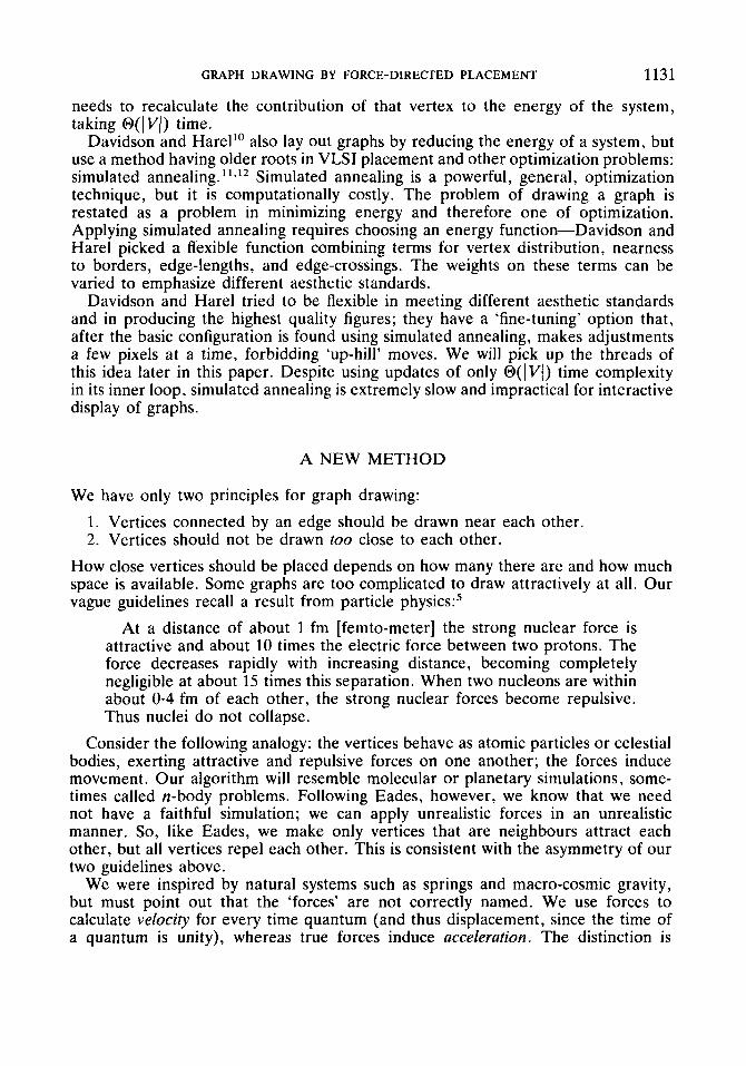
At a distance of about 1 fm [femto-meter] the strong nuclear force is attractive and about 10 times the electric force between two protons. The force decreases rapidly with increasing distance, becoming completely negligible at about 15 times this separation. When two nucleons are within about 0-4 fm of each other, the strong nuclear forces become repulsive. Thus nuclei do not collapse.

Consider the following analogy: the vertices behave as atomic particles or celestial bodies, exerting attractive and repulsive forces on one another; the forces induce movement. Our algorithm will resemble molecular or planetary simulations, some- times called n-body problems. Following Eades, however, we know that we need not have a faithful simulation; we can apply unrealistic forces in an unrealistic manner. So, like Eades, we make only vertices that are neighbours attract each other, but all vertices repel each other. This is consistent with the asymmetry of our two guidelines above.

We were inspired by natural systems such as springs and macro-cosmic gravity, but must point out that the 'forces' are not correctly named. We use forces to calculate velocity for every time quantum (and thus displacement, since the time of a quantum is unity), whereas true forces induce acceleration. The distinction is

1132 T. M. J . FRUCHTERMAN A N D E. M. REINGOLD

extremely important, because the real definition leads to dynamic equilibria (pendulums, orbits), and we seek static equilibria.

Pseudo-code for the algorithm is given in Figure 1. We have not said anything about the initial configuration, the input, or the output. The initial configuration could be all or partly specified, but normally vertices are placed randomly in the frame. Different functions might have been chosen for fu and fr.

There are three steps to each iteration: calculate the effect of attractive forces on each vertex, then calculate the effect of repulsive forces, and finally limit the total displacement by the temperature. A special case occurs when vertices are in the same position: our implementation acts as though the two vertices are a small distance apart in a randomly chosen orientation: this leads to a violent repulsive effect separating them.

Figure 1 omits an explanation of ‘temperature’ and ‘cooling’. The idea is that the displacement of a vertex is limited to some maximum value, and this maximum value decreases over time; so, as the layout becomes better, the amount of adjustment becomes finer and finer. For example, the temperature could start at an initial value

urea := W * L; { W and L are the width and length of the frame } G := (V, E); { the vertices are assigned random initial positions } 12 ~4-1 function fo(x) := begin r e t u r n z 2 / k end ; function fi(x) := begin r e t u r n k 2 / z end;

for i := 1 to iferutions do begin { calculate repulsive forces } fo r v in V do begin

{ each vertex has two vectors: .pos and .disp } v.disp := 0; for u in V do

if (u # v) then begin { A is short hand for the difference} { vector between the positions of the two vertices }

v.disp := v.disp+ (A/lAl) * fr(lAl) A := U.~OS- U.PS;

end end

{ calculate attractive forces } fo r e in E do begin

{ each edge is an ordered pair of vertices .v and .u } A := e.v.pos - e.u.pos; e.v.disp := e.v.disp - (A/(A() * fe(lAl); e.u.disp := e.u.disp+ (A/lAl) * fo(lAl)

end

{ limit the maximum displacement to the temperature 1 } { and then prevent from being displaced outside frame } for v in V do begin

u p s := v.pos+ (v.disp/lu.displ) * min(v.disp,t); v.pos.x := min(W12, maz(-W/2,v.pos.z)); v.pos.y := min(LI2, ma.(- Li2, u.pos.y))

e n d { reduce the temperature as the layout approaches a better configuration } t := cool(t)

e n d

Figure I . Force-directed placement


(say one tenth the width of the frame) and decay to 0 in an inverse linear fashion. We discuss more efficient cooling functions later.

Modelling the forces We calculate k , the optimal distance between vertices as

= d( number area of vertices 1 where the constant C is found experimentally. We would like the vertices to be uniformly distributed in the frame, and k is the radius of the empty area around a vertex. Intuitively, the further apart two vertices are, or the closer together, the more overpoweringly intolerable the current layout should be considered and the more violent the correction. If f a and f r are the attractive and repulsive forces, respectively, with d the distance between the two vertices, then

fa(d) = d2/k fr(d) = -k2/d

Figure 2 illustrates these forces and their sum versus distance. The point where the sum of the attractive and repulsive force crosses the x-axis is where the two forces would exactly cancel each other out, and this is at k , the ideal distance between vertices.

Distance fi

Figure 2. Forces versus distance


We chose the two functions fu and f r after some experimentation; they naturally suggested themselves as implementing our objectives, and they resembled Hooke’s law. We experimented with several other functions that seemed to meet our guidelines, for example

f u (d ) = d/k fr(d) = -k/d

This latter pair of functions, however, worked poorly for more complex graphs because it seemed unable to overcome local minima; a vertex was less likely to move past another vertex that a bad initial placement had put in its way. Overcoming a bad configuration by moving through a yet worse configuration before reaching a better one is known in simulated annealing as hill climbing. Simulated annealing decides probabilistically whether to accept a transition to an inferior configuration, but our force-directed placement always seeks the lowest ground. This would lead to getting stuck in local minima or ‘valleys’ more often, except that our simulation is discrete, and a vertex can shoot past another in a single time step without having to face its repulsive effects at short range, where they would be inexorable. Force laws that use higher order powers tend to give results similar to those of the quadratic functions, but are more costly to compute.

Eades’ equations were

We achieved results similar to those of Eades, as we will show, but we rejected his formula for fu since it was inefficient to compute.

The frame

We have to confine the graph to the frame specified by the user. Originally, we placed dummy vertices around the perimeter of the graph that exerted repulsive forces but could not move themselves. Exactly the same strategy occurred at first to Davidson and Harel. They then modelled the walls as a sloping potential barrier, by putting a term in their energy function causing the cost for a vertex being near a border to increase inverse-quadratically. We chose to consider the frame an immovable object, modelling it as four walls, each of which exerts a normal force exactly equal to the force pushing any vertex beyond it, thus stopping it like a real wall.

We have yet to implement satisfactorily an extension of this concept to borders constructed of arbitrary line segments. For example one might try to draw a tree inside a wedge-shaped area by fixing the root of the tree at the apex of the wedge. In drawing a graph within a concave region, we must prevent edges as well as vertices from crossing borders. This adds a term of @ ( I VllEl) to the time complexity of our algorithm, but such arbitrary regions would be useful for reserving an island for text in the middle of a graph.


There are several approaches for modelling the frame after physical walls. The easiest is the ‘sticky’ vertex that adheres to the spot on the wall where it first strikes (an inelastic collision) and stays there until the force vector on it has only components moving away from the wall (see Figure 3) . Another approach is to model striking the wall as an elastic collision but then we must determine the order in which the walls are struck-and perhaps a vertex would ‘bounce’ many times, entailing extensive computation (see Figure 4). This approach is reminiscent of ray tracing,13 a realistic but computation-intensive method used for shading in computer graphics.

We chose to have a wall stop that component of displacement normal to it. This was easy and efficient to implement for a box around the graph because all the walls are orthogonal to the co-ordinate system. Figure 5 shows a vertex stopped in its proposed trajectory outside the frame by the top border, but in Figure 6 the vertex is allowed to slide along to the left until it reaches the left border and lodges in the upper left corner. (For borders made of arbitrary lines, we would have to compute dot products to find the component of the trajectory normal to the border.) In practice, we often choose the strength of the forces so that the resulting graph is small enough that it never nears the borders, then apply a filter to enlarge the graph to fill the frame.

Speeding up the algorithm An important technique in n-body simulations is to approximate the effect of

distant bodies as a single pole.’4 Doing this reduces the n-body simulation from @(n2) complexity to O(n log n). We need not faithfully imitate a celestial, chemical, or atomic system-we desire only that the results be pleasing. This allowed us to

Figure 3. Inelastic collision Figure 4. Elastic collision

1136 d

T. M. J . FRUCHTERMAN AND E. M. REINGOLD

0.-

x-componen

...... '

Figure 5. Halted in upward direction Figure 6. Stopped altogether

make one time-saving adjustment already described: vertices are only attracted to their neighbours-this has O( 1 El) complexity. Still, we have to compute the repulsion of every vertex from every other; this has O(lV12) complexity. The repulsive force decreases as the inverse square of the distance. Can we neglect the contribution of the more distant vertices?

To speed up our algorithm we used a variation that we call the grid-variant algorithm. In this variant we divide the screen into a grid of squares, and at each iteration, each vertex is placed in its grid square and repulsive forces are computed only between it and the vertices in nearby squares of the grid; we compute the attractive forces as usual. This is nearly equivalent (in the resulting output, if not the time complexity) to applying the repulsive force to all vertices, but computing it as

k2 ' d f = - 4 2 k - d )

where

1 , i fx > 0 0, otherwise u(x) =

In practice, we found that the square shape of the grid boxes caused distortion, and it was necessary to make the fall-off distance the same in all directions (the repulsive force is applied from all vertices within the circular area of radius 2k centred at the centre of the vertex in question). In Figure 7, vertex v is repelled from vertex q ,

1137

I I I I I I I I I . $ I I I

- 2k 3 Figure 7. Calculating repulsive forces using the grid-square algorithm

but not from r , which is outside the immediately neighbouring squares of the grid, or s, which is considered but then rejected for being too far away anyway.

If the frame has width W and length L, then the area per vertex is

and again

k = JA

Because we ignore the repulsion of vertices beyond a distance of 2k, 2k is the length of a side of a grid box.

W L Ivl IVI 2k 2k 4 w L - 4

Number of grid boxes = - -- = W L __

When the distribution of vertices is approximately uniform, then the calculation of the repulsive force becomes @(I V l ) .

An important consideration of simulated annealing is choosing a cooling schedule for the temperature T , balancing the ability to escape local minima and find the best layout with the desire for quick termination. Our analogue to simulated annealing’s temperature is limiting the maximum displacement of every vertex during an iteration, and changing that maximum displacement from iteration to iteration.

Much research in simulated annealing is devoted to speeding it up, much of the effort goes into developing better and more general cooling schedules. Sirnuluted sintering is a variant on simulated annealing that is based on the hypothesis that simulated annealing wastes effort in moving from a random placement to a reasonable one, and that it would be better to generate a good initial placement by applying a


more computationally efficient method and then apply simulated annealing at a low temperature to make more subtle adjustments. 1 2 . l 5 Indeed, this resembles what Davidson and Harel have done, with their computation-intensive final adjustment phase. GroverI5 suggests min-cut placementI6 for initial VLSI layout. Another alternative for quickly generating an initial layout is quenching, simulated annealing rapidly cooling over a few iterations. To keep our system conceptually simple, we do something analogous to simulated sintering, but we will use the force-directed analogy to quenching to avoid introducing another algorithm.

We conducted some subjective experiments in which we compared the results of drawing different graphs under different cooling schedules and using different num- bers of iterations. Primarily, we compared a steady decrease in temperature with a combination of quenching and simmering: the first phase starts at a high temperature and cools steadily and rapidly, and the second is at a constant low temperature. The results from the latter schedule were better and required fewer iterations.

Time complexity Each iteration of our algorithm takes time @(IV1* + IEI) for the basic algorithm

and O(lVl) + IEI) for the grid variant, assuming that vertices are uniformly distributed over the grid boxes; but exactly how many iterations are necessary to lay out a graph attractively? There is much ad hoc argument in the literature when the authors try to explain when the algorithm terminates. Eades simply asserted that ‘Almost all graphs reach a minimal energy state after the simulation step is run 100 times’. Davidson and Harel, and Kamada and Kawai, based conditions for termination on their explicit representations of state energy but they offered little analysis how soon those conditions would be met; indeed, Kamada and Kawai did not include the number of iterations in their outermost loop in doing their time complexity analysis! We too can offer little justification for the number of iterations, although we experimented with making it a function of IVI or [ E l . We did suspect, as did Davidson and Harel, that choosing a better cooling schedule could make a dramatic difference.

The algorithms that attempt to minimize energy terminate when an energy threshold is reached. In contrast, our algorithm’s termination is guesswork, as was Eades’. However, the intermediate output of the program can be saved and used as an initial configuration if the layout comes out ‘half-baked’, and then more simmering can be used to fix the layout for less cost than starting from scratch. Also, saving the intermediate layout facilitates other forms of incremental layout, such as adding edges or vertices to a graph already laid out.

IMPLEMENTATION We wanted to have a simple, coherent method, not a bag-of-tricks. For example, we rejected planarity testing and planarization even though they are efficient. We avoided slow, complicated techniques such as simulated annealing, and we tried to make our implementation fast enough to be interactive for graphs of moderate size.

We constructed a flexible experimental framework, to let us easily test many different models of forces. We could specify arbitrarily complex functions using addition, subtraction, multiplication, division, modulus, logarithm, square root,


exponentiation, and the unit step function in an AWK-like syntex” on the command line.

We implemented our algorithm in C + +. 18, ’’) We used integer arithmetic for speed; this often required that expressions be carefully crafted to preserve significance, but it proved worth while. Following the advice of Bentley,“ we kept expensive operations such as square roots to a minimum; often a square will do in the place of a square root. Experimentation was aided by the ‘little language’ used to specify the forces and other parameters. Many an idea was evaluated this way, and then hard-coded if it proved its worth (such as the grid approximation and sintering).

There are several variants of the lay-out program. The basic version is called Nature because of the analogy between our layout algorithm and the forces of nature. We have a variant that lays out in three dimensions, called Nature3d’ and the one that implements the grid variant called Naturev. All three take text input and produce text output. The input file format is the same as that of the output, except that the input will not necessarily have co-ordinates for the points. If it does, those specify the initial configuration, otherwise vertices are placed randomly. So, if one pass through Nature fails to result in a pleasing layout, one can resubmit the graph, but now some computation is saved because one can reuse the output of the first attempt. The difference between the variants is a matter of linking to different object files.

AN EXTENDED EXAMPLE-THE PENTAGONAL PRISM To demonstrate our algorithm in action, we show in Figures 8 and 9 every step in laying out a pentagonal prism. The first frame shows all the vertices in their random initial positions. The first twelve frames show quenching; the second twelve, simmering.

In general throughout this paper, if a figure has a box around it, that box is the border that is part of our algorithm. Most figures have no box, which means they have been scaled by a filter. We identify all graphs in figure captions by giving the figure number in the original paper and the citation. Some are specially identified with ‘as drawn by’ or ‘as proposed by’; these are reproductions of those figures exactly as they appeared in the cited paper. ‘As drawn by’ identifies those representations produced by the algorithm discussed in the cited paper, whereas ‘as proposed by’ identifies those that were merely proposed by the authors, but not generated by their algorithm.

SYMMETRIC GRAPHS The most natural and pleasing results from our algorithm are those from highly symmetric graphs in which the underlying force-law paradigm is most evident. One such symmetric graph, ubiquitous in papers on graph layout, is K5 (Figure 10). K5 and the other complete graphs K4 (Figure l l ) , Kh (Figures 12 and 13), and K8

(Figure 14), illustrate the balance of attractive and repulsive forces in equilibrium. Note that K4 is planar but has not been represented so. The layouts of complete graphs get smaller as the degree gets higher: the higher the density of edges, the shorter the distances at which equilibrium is reached. Our calculation of the ideal distance between vertices works as we ideally described it only in the simple case of


2 1 3

A

4

1 ’

10

fjo

8

11

@:

6

P 9

12 p Figure 8. Quenching


13 14

16

@A

19

@A

I 22

17

20

23

1s - 1

18

21

@ A

24

@A

Figure 9. Simmering

Figure I I . Kq

Figure 12. K h v Figure 13. K h

Figure 14. K x Figure 15. K z


K2 (Figure 15), but since all our figures have been through the enlarger filter, they are all of about the same size.

Some more examples of simple, planar or nearly planar, symmetric graphs are the three in Figure 16 and the one in Figure 17, which first appeared in Kamada and Kawai,8 and Figure 18, which appears in Davidson and Harel. '" The graphs presented by Kamada and Kawai are especially easy to draw and our renderings are essentially the same as theirs.

Another highly symmetric graph is K3,3 (Figures 19 and 20). The first representation, although acceptable, is arguably not as good as the other ones because one dimension of symmetry is missing. The Heywood graph (Figure 21) was taken from Davidson and Harel, but they did not achieve this drawing with their algorithm: their layout is Figure 22. Still, it is probably preferable to our Figure 23.

Figure 16. Graphs in Figures 6(a) , 4, and 3, respectively, from Kamada and KawaiX

Figure 17. Triangulated triangle (graph in Figure 6(c) from Kamada and Kawai')

Figure 18. Graph in Figure 16 from Davidson and Harel'"


Figure 19. K3.3 Figure 20. K3.3

Figure 21. Figure 18(a) from Davidson and Harel'" as proposed by Davidson and Harel

Figure 22. Figure 18(b) from Davidson and Harel'" as drawn by Davidson and Harel

Figure 23. Heywood graph (graph in Figure I8 from Davidson and Haref"))


Other difficulties that our algorithm encounters, even with symmetric graphs, are illustrated by Figure 24, which was the first figure of Davidson and Harel."' The original, Figure 25, makes the problem a bit clearer. The graph is planar and Davidson and Harel generated a planar representation, but the repulsive forces from the inner vertices prevent us from achieving the more attractive, yet equally stable, configuration.

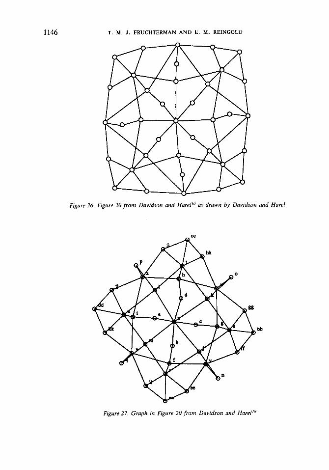
The centrepiece of Davidson and Harel's paper was Figure 26. Our rendition, Figure 27, is faulty in one respect: Davidson and Harel drew the outermost vertices p , q, n and o between their two neighbours to make the graph perfectly planar. As a comparison, using the time complexity formula Davidson and Harel provide, they would require 10 minutes to generate the figure, but our algorithm takes 30 seconds on a comparable machine.

Figure 28 displays two different layouts of an icosahedron missing one vertex and its incident edges; the upper layout looks something like the traditional solid representation of the icosahedron (but with a vertex missing) and the lower layout is planar but some edges are hard to distinguish. Of all the methods we have discussed, only the simulated annealing of Davidson and Harel explicitly attempts to avoid occluding vertices with edges.

Figure 29 is the icosahedron. The layout is extremely attractive, although not planar (the icosahedron is planar).

PLANAR GRAPHS In this section we reproduce, with little comment, some of the asymmetrical figures from other papers that we found easy to draw; almost all these graphs are planar. The layout we produce for each figure is nearly identical to the layout from the paper we cite as the source of the graph.

Figure 24. Graph in Figure I from Davidson and Harel'"

Figure 25. Figure 1 from Davidson and Harel" as drawn by Davidson and Harel

1146 T. M. J . FRUCHTERMAN AND E. M. REINCOLD

Figure 26. Figure 20 from Davidson and Harel'" as drawn by Davidson and Harel

Figure 27. Graph in Figure 20 from Davidson and Harel'"


Figure 29. Icosahedron

Figure 28. Two layouts of an icosahedron variant

Figure 30. Graphs in Figures 7(c), 7(a) and 7(d) from Kamada and Kawai'

Figure 31. Graph in Figure 2(b) from Eades'


b

Figure 32, Graph in Figure 5(c) from Eades’ Figure 33. Graph in Figure 5(b) from Eades’

Figure 34. Graph in Figure 5(a) from Eades’ Figure 35. Graph in Figure 6(c) from Eades-’

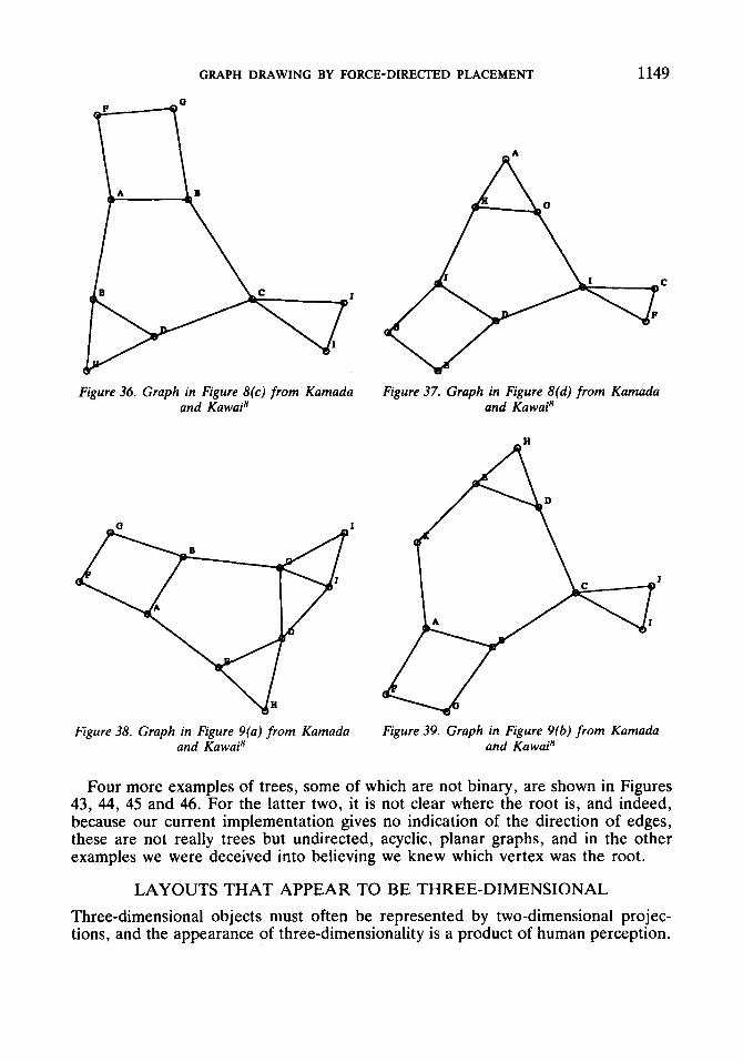
Kamada and Kawai observed that isomorphic graphs, such as those in Figures 36 and 37, will have identical layouts, up to rotation and reflection, whereas similar but not isomorphic graphs, such as in Figures 38 and 39 will have similar but distinct layouts. Our results confirm with this observation.

A simple binary tree is represented in Figure 40. Our algorithm draws trees as expanding radially from the root, as do many other algorithms. Some of the problems with our algorithm, which does not directly penalize edge crossings, are illustrated by Figure 41. Here, the children of the second level cross each other because that placement packs the vertices in the frame. A similar problem that occurred in an early implementation of our algorithm, but to a more serious degree, was the blocking affect illustrated in Figure 42. Vertices aaab, aaaba and aaabb are attracted to ancestor ma, but cannot overcome the potential barrier posed by vertices ab and aba. We tried to find an analogy in nature that would suggest a way that such a blocking force could be overcome. Quantum jumps by electrons came to mind, but the heuristic we used to solve this problem was to turn off the repulsive force every fifth iteration. This heuristic is helpful, but it cannot overcome a problem that involves many vertices such as in Figure 41. We suspect that if we apply a multi- grid technique that allows whole portions of the graph to be moved, it might be of some help, but such a technique would be more suitable for an optimization algorithm such as simulated annealing.


Figure 36. Graph in Figure 8(c) from Kamada and Kawain

Figure 37. Graph in Figure 8(d) from Kamada and Kawain

Figure38. Graph in Figure 9(a) from Kamada and KawaiX

Figure 39. Graph in Figure 9(b) from Kamada and KawaiX

Four more examples of trees, some of which are not binary, are shown in Figures 43, 44, 45 and 46. For the latter two, it is not clear where the root is, and indeed, because our current implementation gives no indication of the direction of edges, these are not really trees but undirected, acyclic, planar graphs, and in the other examples we were deceived into believing we knew which vertex was the root.

LAYOUTS THAT APPEAR TO BE THREE-DIMENSIONAL Three-dimensional objects must often be represented by two-dimensional projections, and the appearance of three-dimensionality is a product of human perception.


Figure 40. Binary tree Figure 41. Tangled binary tree (graph in Figure 14(a) from Davidson and Harel"')

Figure 42. Example of a potential barrier

An example of a graph that looks three-dimensional when drawn by our algorithm, and by the other algorithms we have discussed here, is the cube of Figure 47. Although it can be drawn as a planar graph (the planar representation can also be viewed as the head-on perspective projection of an opaque cube), a human being would rarely want to do so. We take a further step and attempt to draw a hypercube, which is shown in Figure 48. The layout is good, but it is difficult to picture the original four-space object.

Davidson and Hare1 tuned their algorithm by changing the weighting of various components. In an attempt to produce a planar rendition of the cube, they experimented with more heavily weighting the term penalizing edge-crossings and were

GRAPH DRAWING BY FORCE-DIRECTED PLACEMENT 1151 Q

Figure 43. Tree (graph in Figure 4(a) from Eades') Figure 44. Tree (graph from Figure 14(b) from Davidson and HareP)

Figure 45. Graph in Figure 7(b) from Kamada and Kawai'

Figure 46. Unbalanced tree (graph in Figure from Eades')

able to draw the cube as two squares, one inside the other, but with the inner square rotated with respect to the outer one because that made the edge lengths more uniform. Two other graphs that are planar but are usually drawn as three-dimensional are the pentagonal prism (Figure 49) and the twin cubes (Figure 50). Davidson and Harel also tried to make these graphs planar, but they failed in the latter case. Figure 51 is the planar layout they sought. Figure 52 was the result of weighting the edge crossing component more favourably, but it has just as many crossings as Figure 53, the layout produced by their default settings. However, Figure 52 does give the effect of being a perspective projection.

Davidson and Harel did an extended example on Figure 54, except that in their paper it appeared planar and like a closing shutter (Figure 55). Once again, our


Figure 47. Cube

Figure 48. Four-dimensional hypercube

representation appears to be an oblique parallel projection of an object, whereas Davidson and Harel have something like a perspective projection (their algorithm adds a twisted effect to keep edge lengths nearer uniform).

Kamada and Kawai, and Davidson and Harel, discussed how their algorithms draw isomorphic graphs in the same way, though perhaps rotated and reflected. Apparently, both papers were referring to rotation and reflection in the plane, but we were struck by how our algorithm appears to rotate graphs that are three- dimensional-looking graphs in three space. Examples are the dodecahedra of Figures 56 and 57. The algorithm produced different results because of different initial configurations. The layout in Figure 56 is not nearly as acceptable in appearance as the two in Figure 57.

THREE-DIMENSIONAL LAYOUT Our layouts that appeared three-dimensional led us to experiment with doing the layout in three dimensions and projecting the result obtained onto two dimensions; in this way we hoped to obtain more control over the final image. As we saw with the dodecahedron, the algorithm can generate different ‘projections’ of the same object, depending on initial placement and the cooling schedule, and the projection might be ‘bad’ because it occludes edges and vertices and hides planes that are being viewed with a view normal vector that is parallel, or nearly so, to those planes. We created another filter to do projections of vertices laid out in three dimensions onto two, with options to choose the view reference point, view normal vector, and view up vector, with choice of parallel or perspective projection (see Hearn and BakerI3 for definitions of these terms).

We now show some examples repeated from previous sections, but now laid out in three dimensions. Each example is a triplet of projections from the x , y and z axes.


Figure 49. Pentagonal prism

Figure 50. Twin cubes (graph in Figure 11 from Davidson and Harel"')

Figure 51. Figure I l ( a ) from Davidson and HareP as proposed by Davidson and Harel

Figure 52. Figure I l (b ) from Davidson and Harel") as drawn by Davidson and Harel

Figure 53. Figure I I (c) from Davidson and Harel") as drawn by Davidson and Harel


Figure 54. Mesh (graph in Figure 2 from -

as drawn by Davidson and Harel Davidson and Harel"')

Figure 56. Poor dodecahedron

Figure 57. Good dodecahedron


The first examples are the cube (Figure 58) , the mesh (Figure 59), and the pentagonal prism (Figure 60). Examining the dodecahedron (Figure 61), the icosahedron (Figure 62), and the twin cubes (Figure 63), we see the possibility for a good projection, but there is no guarantee that any projection will necessarily be better than the one we can get from laying out the graph in two dimensions. Calculating a projection from the layout has little cost, but currently requires intervention by the user to choose a projection. A better interface would allow the user interactively to manipulate the object in three dimensions. Kamada and KawaiZ0 discuss the problem of selecting the ‘general position’ for viewing a three-dimensional object so that the maximum shape information is obtained, and presents an algorithm for doing so.

When Davidson and Hare1 tried to find a planar layout for the icosahedron, they also tried Figure 64, the icosahedron missing one vertex and its incident edges. This modification of the icosahedron is clear from our three-dimensional layout.

If a graph appeared to be three-dimensional when laid out by the two-dimensional version of our algorithm, it laid out well in three dimensions; but in general, if it did not look three-dimensional originally, it did not benefit from being laid out in three dimensions, and in fact, the z-orientation of vertices often appeared random and unpleasant. The triangulated triangle of Figure 65, appears to be nearly flat. The graph in Figure 66, which we saw earlier in Figure 18, might be described as

Figure 58. Three-dimensionai layouis of a cube

Figure 59. Three-dimensional layouts of a mesh


Figure 60. Three-dimensional layouts of a pentagonal prism

Figure 61. Three-dimensional layouts of a dodecahedron

Figure 62. Three-dimensional layouts of an icosahedron

an ‘iterated K4’: K4 with copies of K4 attached to each vertex. Here it looks like a monstrosity. K6 (Figure 67) is rendered as an octahedron with internal edges; it compares unfavourably with the icosahedron and the other graphs that had no lines ‘under’ the surface. The third projection, along the z-axis, does not appear three- dimensional. K8 (Figure 68) is a mess.

We have already seen the mesh and the twin cubes rendered in three dimensions. Davidson and Hare1 attempted to make the twin cubes planar by increasing the cost of edge crossings in their energy function. They failed, but they did produce a


Figure 63. Three-dimensional layouts of twin cubes

Figure 64. Three-dimensional layouts of an icosahedron variant

Figure 65. Three-dimensional layouts of a triangulated triangle

drawing that resembled a perspective projection. Given the three-dimensional layout of both the mesh and the twin boxes, we can choose a view normal vector that gives us a perspective projection that appears planar. These are shown in Figure 69 and Figure 70. It required human intervention to choose the view normal vector.

In summary, a three-dimensional layout stands or falls according to the preference and expectations of the user. A graph that is ‘really’ three-dimensional ought to be laid out in three dimensions, and the user ought to be able to manipulate this three-


Figure 66. Three-dimensional layouts of ‘iterated Kq’

Figure 67. Three-dimensional layouts of KO

Figure 68. Three-dimensional layouts of KH

dimensional layout with natural operations, such as choosing the viewpoint, direction of the view and projection.

GRID VARIANT We must deal with a problem faced by Kamada and Kawai (and presumably Eades): disconnected graphs have nothing to hold them together; the connected components fly apart and flatten themselves against the walls-an example is Figure 71. The


Figure 69. Planar appearing perspective projection Figure 70. Planar appearing perspective projection of mesh of twin cubes

Figure 71. Disconnected graph (graph in Figure 3(b) from Davidson and HarePo)

Figure 72. Twin Ks

obvious solution is mentioned in Kamada and Kawai: partition the graph into its connected components (this is easily done in linear time2') and give each component a region of area proportional to its size, with each component laid out independently; Kamada and Kawai did not implement this. Without explicitly testing for connec- tedness or finding the connected components, we achieve this 'regional' effect as an added benefit of using the grid-square variant of our algorithm. We will also benefit when drawing nearly disconnected graphs such as the twin copies of Ks connected by a single strand in Figure 72. Each clique acts as a repulsive centre that pushes


all the vertices in the other clique far away and stretches the solitary connection. This rendering is acceptable, but the separation is perhaps a bit exaggerated.

The advantage of the grid variant of our algorithm is that distant vertices do not repel. We get almost the same effect as we would by separating the components (see Figures 73 and 74). At first, the connected components drift apart from one another, but eventually they get out of each other’s range and settle down. The connected graph improves in similar ways: the two cliques are not as distant as before and each is less distorted by the influence of the other.

There is considerable overhead involved in placing each vertex in a grid square each iteration and so we expect that the algorithm is more useful for larger graphs. In general, we found to our annoyance that the grid variant was neither distinctly better nor distinctly worse than the basic algorithm, which is why we have presented both.

The grid variant (Figure 76) appears ‘fluffier’ than either Figure 75, produced by the basic algorithm, or than the original from Eades, sketched in Figure 77, although it has unnecessary edge crossings unlike the other two. A similar triplet is Figures 78, 79, and 80. We are not sure why Eades has a kink in his drawing; this could depend on initial placement.

The remaining figures show the layout produced by the basic algorithm on the left and that of the grid variant on the right. The symmetry of a large graph can be marred, as in Figure 81. The symmetry on the large scale requires that each vertex be placed with respect to every other vertex, or every vertex must be calculated into the forces acting on every other. The tree in Figure 82 has more uniform edge lengths and better use of space when laid out by the grid algorithm. The grid algorithm is in general faster for the larger graphs, but requires more iterations. Fifty iterations and 8 seconds produced the layout on the left in Figure 83, and 70 iterations and 6 seconds produced the one on the right.

Figure 73. Grid-variant layout of twin Ks

Y Figure 74. Grid-variant layout of disconnnected graph (graph in Figure 3(b) from Davidson and

HareP’)


A D

Figure 75. Graph in Figure 6(a) from Eades-’ Figure 76. Grid-variant layout of graph in Figure 6(a) from Eades’

Figure 77. Figure 6(a) from Eades’ as drawn by Eades

CONCLUSIONS The primary advantage of our algorithm is speed. Many of the graphs were drawn in less than a second, and all were drawn in under 10 seconds on a SPARC station 1. We consider this to be ‘interactive’ speed.

Davidson and Harel’s algorithm appears to be able to attain a slightly higher level of aesthetics and flexibility for the more complex graphs. Probably they could also lay out graphs using a three-dimensional variant and use a grid, or multi-level approach, but then again, they face more complexities of implementation and pay a higher penalty in running time.


Figure 78. Graph in Figure 6(b) from Eades’ Figure 79. Grid-variant layout of graph in Figure 6(b) from Eades’

Figure 80. Figure 6(b) from Eades’ as drawn by Eades

A major goal was that the algorithm should work reasonably well almost always, without the user having to fiddle with options, change the force laws, increase the number of iterations, or switch to three-dimensional variants. Because we had no explicit concept of energy, and hence could not detect a stopping condition, we simply used 50 iterations every time; this was excessive on the simpler graphs, but that did not matter since the smaller graphs take less time per iteration in any case and the algorithm is so fast.

1163

Figure 81. Graph in Figure 1

Q

from Davidson and Harel'"

Figure 82. Graph in Figure 14(a) from Davidson and Harei'"

Figure 83. Square grid (graph in Figure 13 from Davidson and Harel'")

1164 T. M. J. FRUCHTERMAN AND E. M. REINGOLD

REFERENCES 1. F. Harary, Graph Theory, Addison-Wesley, Reading, MA, 1969. 2. P. Eades and R. Tamassia, ‘Algorithms for drawing graphs: an annotated bibliography’, Networks,

3. P. Eades, ‘A heuristic for graph drawing’, Congressus Numerantium, 42, 149-160 (1984). 4. N. Quinn and M. Breur. ‘A force directed component placement procedure for printed circuit

5. P. A. Tipler, Physics, 2nd edn, Worth Publishers, New York, 1982. 6. J. Bentley, Programming Pearls, Addison-Wesley, Reading, MA, 1986. 7. L. Greengard, The Rapid Evaluation of Potential Fields in Particle Systems, MIT Press, Cambridge,

MA, 1988. 8. T. Kamada and S. Kawai, ‘Automatic display of network structures for human understanding’,

Technical Report 88-007, Department of Information Science, Tokyo University, February, 1988. 9. T Kamada and S. Kawai,‘An algorithm for drawing general undirected graphs’, Information

Processing Letters, 31, (l) , 7-15 (1989). 10. R. Davidson and D. Harel, ‘Drawing graphs nicely using simulated annealing’, Technical Report

1389-13, Department of Applied Mathematics and Computer Science, The Weizmann Institute, Rehovot, Israel, July, 1989. A revised version, dated April, 1991, has been submitted to Communi- cations of the ACM.

11. S. Kirkpatrick, C. D. Gelatt and M. P. Vecchi, ‘Optimization by simulated annealing’, Science, 220, (4598), 671480 (1983).

12. R. Otten and L. van Ginneken, The Annealing Algorithm, Kluwer Academic Publishers, Boston, MA, 1989.

13. D. Hearn and M. P. Baker, Computer Graphics, Prentice-Hall, Englewood Cliffs, NJ, 1986. 14. A. Appel, ‘An efficient algorithm for many-body simulations’, SIAM Journal on Scientific and

15. L. K. Grover, ‘Standard cell placement using simulated sintering’, Proceedings 24th Design Auto-

16. M. A. Breuer, ‘Min-cut placement’ Journal of Design Automation and Fault Tolerunt Computing,

17. B. W. Kernighan, A. V. Aho and P. J. Weinberger, The AWK Programming Language, Addison-

18. B. Stoustrup, The C+ + Programming Language, Addison-Wesley, Reading, MA, 1986. 19. S. C. Dewhurst and K. T. Stark, Programming in C++, Prentice-Hall, Englewood Cliffs, NJ,

20. T. Kamada and S. Kawai, ‘A simple method for computing general position in displaying three-

21. E. M. Reingold, J. Nievergelt and N. Deo, Combinatorial Algorithms: Theory and Practice,

to appear.

boards’, IEEE Trans. on Circuits and Systems, CAS-26, (6), 377-388 (1979).

Statistical Computing, 6, ( l ) , 85-103 (1985).

mation Conference, 1987, pp.56-59.

1, (4), 343-382 (1977).

Wesley, Reading, MA, 1989.

1989.

dimensional objects’, Computer Vision, Graphics, and Image Processing, 41, 43-56 (1988).

Prentice-Hall, Englewood Cliffs, NJ, 1977.

graph drawing by force-directed placement - reingold · graph drawing by force-directed placement...

Documents