USE OF ULTIMATE LOAD THEORIES FOR DESIGN

OF DRILLED SHAFT SOUND WALL FOUNDATIONS

Matthew Justin Helmers

Thesis submitted to the Faculty of theVirginia Polytechnic Institute and State University

in partial fulfillment of the requirements for the degree of

MASTER OF SCIENCE

in

Civil Engineering

J. Michael Duncan, ChairGeorge M. Filz

Thomas L. Brandon

June 20, 1997Blacksburg, VA

Keywords: Lateral Loads, Drilled Shafts, Field Load TestsCopyright 1997, Matthew J. Helmers

ii

USE OF ULTIMATE LOAD THEORIES FOR DESIGN OF DRILLED SHAFT SOUND WALL FOUNDATIONS

Matthew Justin Helmers

(Abstract)

A study was performed to investigate the factors that affect the accuracy of theprocedures used by the Virginia Department of Transportation for design of drilled shaftsound wall foundations. Field load tests were performed on eight inch and nine inchdiameter drilled shafts, and the results were compared to theoretical solutions for ultimatelateral load capacity. Standard Penetration Tests were run in the field and laboratorystrength tests were performed on the soils from the test sites. It was found that publishedcorrelations between blow count and friction angle for sands and gravels can be used toestimate friction angles for the partly saturated silty and clayey soils encountered at thetest sites. A spreadsheet program was developed to automate the process of determiningdesign lengths for drilled shaft sound wall foundations. The spreadsheet was used toinvestigate the effects of different analysis procedures and parameter values on the designlengths of drilled shaft sound wall foundation.

iii

ACKNOWLEDGMENTS

The writer wishes to thank Professor J. M. Duncan for his contributions to all aspects

of this research. He was a continuous source of ideas pertaining to the experimental

aspects and the practical applications of the research. His help and guidance in preparing

this manuscript is gratefully acknowledged. His support and encouragement is

appreciated.

Professor Filz’s discussions on areas regarding this research and other areas of

geotechnical engineering were enjoyable and much appreciated. Professor Brandon

helped with instrumentation and data acquisition. He also provided many helpful

suggestions during the development of a loading system. All the committee members are

thanked for reviewing the manuscript.

Thanks to Charles “Andy” Babish for his help in the testing phase of this research and

his friendship throughout the graduate program. It was a pleasure to work with Bob

Mokwa on many aspects of the research. Thanks also to Chris, Diane, Jes£s, and John for

their friendship and discussions related to geotechnical engineering and many other areas.

To all my family, I wish to thank them for their constant support throughout my

educational career.

Financial support for this research was provided by the Virginia Transportation

Research Council in conjunction with the Virginia Department of Transportation. The

author was supported by a Dwight David Eisenhower Fellowship.

iv

TABLE OF CONTENTS

LIST OF FIGURES ................................................................................................. vii

LIST OF TABLES ................................................................................................... ix

CHAPTER 1 - INTRODUCTION ........................................................................... 1

CHAPTER 2 - THEORIES FOR ULTIMATE LATERAL CAPACITIES OFECCENTRICALLY LOADED DRILLED SHAFTS.................................. 3

2.1 Introduction ..................................................................................... 3

2.2 Mechanisms of Deformation and Soil Resistance .............................. 3

2.3 Broms’s (1964a) Theory for Cohesive Soils with φ = 0..................... 4

2.4 Broms’s (1964b) Theory for Cohesionless Soils................................ 6

2.5 Brinch-Hansen’s (1961) Theory for Soils having both Cohesion andFriction............................................................................................. 7

2.6 Use of Ultimate Load Theories to Compute Bending Moments......... 8

2.7 Summary.......................................................................................... 9

CHAPTER 3 - FIELD LOAD TESTS ..................................................................... 10

3.1 Introduction ..................................................................................... 10

3.2 Test Shaft Construction.................................................................... 10

3.3 Loading Equipment .......................................................................... 12

3.4 Loading Procedure ........................................................................... 13

3.5 Test Results...................................................................................... 14

3.6 Summary.......................................................................................... 16

CHAPTER 4 - SOIL PROPERTIES ....................................................................... 18

4.1 Introduction ..................................................................................... 18

4.2 Standard Penetration Tests ............................................................... 18

4.3 Summary of SPT Results .................................................................. 20

4.4 Classification Tests........................................................................... 20

4.5 Summary of Classification Test Results............................................. 24

4.6 Triaxial Tests.................................................................................... 24

v

4.7 Relationships Between φ Values From TriaxialTests and SPT Blow Counts ............................................................... 31

CHAPTER 5 - COMPARISON OF MEASURED AND CALCULATEDULTIMATE LATERAL LOAD CAPACITIES .......................................... 33

5.1 Introduction ..................................................................................... 33

5.2 Broms’s (1964b) Theory .................................................................. 34

5.3 Brinch-Hansen’s (1961) Theory........................................................ 35

5.4 Brinch-Hansen’s (1961) Theory with Cohesion Set Equal to Zero .... 35

5.5 Brinch-Hansen’s (1961) Theory Neglecting Soil Resistance in theTop 1.5 Times Shaft Diameter .......................................................... 35

5.6 Brinch-Hansen’s (1961) Theory, with Calculated CapacitiesMultiplied by 0.85 ............................................................................ 35

5.7 Summary.......................................................................................... 41

CHAPTER 6 - EFFECTS OF ANALYSIS PROCEDURES ANDPARAMETER VALUES.............................................................................. 44

6.1 Introduction ....................................................................................... 44

6.2 Effect of Theory Used in the Analysis ............................................... 44

6.3 Effect of Cohesion............................................................................ 44

6.4 Effect of Sloping Ground.................................................................. 44

6.5 Effect of Ignoring Soil Resistance at the Top of the Shaft ................. 45

6.6 Effect of Soil Friction Angle ............................................................. 45

6.7 Effect of Changing the Factor of Safety ............................................ 45

CHAPTER 7 - CONCLUSION................................................................................ 47

REFERENCES......................................................................................................... 49

APPENDIX A - EQUATIONS FOR Kq AND Kc FACTORS FORTHE BRINCH-HANSEN’S (1961) THEORY............................................. 51

A.1 Introduction ..................................................................................... 51

A.2 Equations for Kq and Kc.................................................................... 51

APPENDIX B - WIND PRESSURES AND WIND LOADSFOR DESIGN OF SOUND BARRIERS...................................................... 54

B.1 Introduction ..................................................................................... 54

vi

B.2 Wind Pressures................................................................................. 54

B.3 Wind Loads...................................................................................... 55

APPENDIX C - DESIGN OF DRILLED SHAFT SOUND WALLFOUNDATIONS USING THE SPREADSHEET LCAP ............................ 58

C.1 Introduction ..................................................................................... 58

C.2 Input for LCAP ................................................................................ 58

C.3 Components of LCAP ...................................................................... 59

C.4 Calculations Performed by LCAP ..................................................... 63

C.5 Sloping Ground Conditions .............................................................. 65

C.6 Output from LCAP........................................................................... 66

VITA ....................................................................................................................... 67

vii

LIST OF FIGURES

Figure 2.1: Mechanism of Deformation of anEccentrically Loaded Drilled Shaft....................................................... 4

Figure 2.2: Broms (1964a) - Assumed Soil Reactionfor Cohesive (φ = 0) Material .............................................................. 5

Figure 2.3: Broms (1964b) - Assumed Soil Reactionfor Cohesionless (c = 0) Material ......................................................... 6

Figure 2.4: Brinch-Hansen (1961) - Assumed Soil Reaction .................................. 8

Figure 2.5: Variation of Kc with Depth .................................................................. 8

Figure 2.6: Variation of Kq with Depth .................................................................. 8

Figure 2.7: Earth Pressure Distributions at Ultimate Loadand One-half of Ultimate Load ............................................................ 8

Figure 3.1: Arrangement of Test Shafts ................................................................. 10

Figure 3.2: Cross-Section of Concrete Shaft.......................................................... 11

Figure 3.3: Test Apparatus .................................................................................... 12

Figure 3.4: Section View of Test Setup ................................................................. 12

Figure 3.5: Plan View of Test Setup...................................................................... 12

Figure 3.6: Typical Load Deflection Curve ............................................................ 14

Figure 3.7: Prices Fork Load Deflection Curves .................................................... 14

Figure 3.8: Salem Load Deflection Curves............................................................. 15

Figure 3.9: Suffolk Load Deflection Curves........................................................... 15

Figure 3.10: Fairfax County Parkway Load Deflection Curves................................. 15

Figure 3.11: Roberts Road Load Deflection Curves................................................. 15

Figure 3.12: Summary of Field Load Tests .............................................................. 16

Figure 4.1: Site Plan, Prices Fork .......................................................................... 18

Figure 4.2: Site Plan, Salem................................................................................... 18

Figure 4.3: Site Plan, Suffolk................................................................................. 18

Figure 4.4: Site Plan, Fairfax County Parkway....................................................... 18

Figure 4.5: Site Plan, Roberts Road....................................................................... 18

viii

Figure 4.6: Summary of Atterberg Limits .............................................................. 20

Figure 4.7a: Prices Fork, Deviator Stress vs. Axial Strain Curves ............................ 27

Figure 4.7b: Prices Fork, Strength Envelope ........................................................... 27

Figure 4.8a: Salem, Deviator Stress vs. Axial Strain Curves .................................... 27

Figure 4.8b: Salem, Strength Envelope.................................................................... 27

Figure 4.9a: Suffolk, Deviator Stress vs. Axial Strain Curves .................................. 27

Figure 4.9b: Suffolk, Strength Envelope.................................................................. 28

Figure 4.10a: Fairfax County Parkway, Deviator Stress vs. Axial Strain Curves ........ 28

Figure 4.10b: Fairfax County Parkway, Strength Envelope........................................ 28

Figure 4.11a: Roberts Road, Deviator Stress vs. Axial Strain Curves ........................ 28

Figure 4.11b: Roberts Road, Strength Envelope........................................................ 28

Figure 4.12: Variation of Friction Angle with NField ................................................. 31

Figure 4.13: Variation of Friction Angle with N1 ..................................................... 32

Figure 4.14: Variation of Friction Angle with (N1)60 ................................................ 32

Figure B.1: Moments and Loads on Sound Wall Foundations due to Wind............. 55

Figure B.2: Example Calculation of Wind Load ..................................................... 56

Figure C.1: Input and Output from LCAP for Sloping Ground Conditions ............. 60

Figure C.2: Input and Output from LCAP for Level Ground Conditions................. 61

Figure C.3: Method 2 for Accounting for Sloping Ground Surface......................... 65

ix

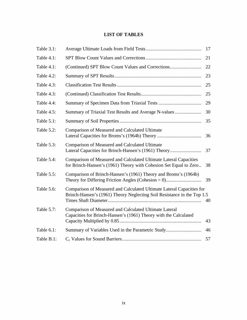
LIST OF TABLES

Table 3.1: Average Ultimate Loads from Field Tests ............................................ 17

Table 4.1: SPT Blow Count Values and Corrections ............................................ 21

Table 4.1: (Continued) SPT Blow Count Values and Corrections......................... 22

Table 4.2: Summary of SPT Results..................................................................... 23

Table 4.3: Classification Test Results ................................................................... 25

Table 4.3: (Continued) Classification Test Results................................................ 25

Table 4.4: Summary of Specimen Data from Triaxial Tests .................................. 29

Table 4.5: Summary of Triaxial Test Results and Average N-values ..................... 30

Table 5.1: Summary of Soil Properties ................................................................. 35

Table 5.2: Comparison of Measured and Calculated UltimateLateral Capacities for Broms’s (1964b) Theory ................................... 36

Table 5.3: Comparison of Measured and Calculated UltimateLateral Capacities for Brinch-Hansen’s (1961) Theory......................... 37

Table 5.4: Comparison of Measured and Calculated Ultimate Lateral Capacitiesfor Brinch-Hansen’s (1961) Theory with Cohesion Set Equal to Zero.. 38

Table 5.5: Comparison of Brinch-Hansen’s (1961) Theory and Broms’s (1964b)Theory for Differing Friction Angles (Cohesion = 0)............................ 39

Table 5.6: Comparison of Measured and Calculated Ultimate Lateral Capacities forBrinch-Hansen’s (1961) Theory Neglecting Soil Resistance in the Top 1.5Times Shaft Diameter .......................................................................... 40

Table 5.7: Comparison of Measured and Calculated Ultimate LateralCapacities for Brinch-Hansen’s (1961) Theory with the CalculatedCapacity Multiplied by 0.85................................................................. 43

Table 6.1: Summary of Variables Used in the Parametric Study............................ 46

Table B.1: Cc Values for Sound Barriers............................................................... 57

1

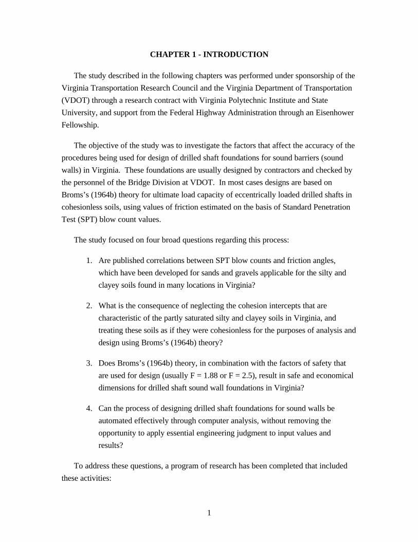
CHAPTER 1 - INTRODUCTION

The study described in the following chapters was performed under sponsorship of the

Virginia Transportation Research Council and the Virginia Department of Transportation

(VDOT) through a research contract with Virginia Polytechnic Institute and State

University, and support from the Federal Highway Administration through an Eisenhower

Fellowship.

The objective of the study was to investigate the factors that affect the accuracy of the

procedures being used for design of drilled shaft foundations for sound barriers (sound

walls) in Virginia. These foundations are usually designed by contractors and checked by

the personnel of the Bridge Division at VDOT. In most cases designs are based on

Broms’s (1964b) theory for ultimate load capacity of eccentrically loaded drilled shafts in

cohesionless soils, using values of friction estimated on the basis of Standard Penetration

Test (SPT) blow count values.

The study focused on four broad questions regarding this process:

1. Are published correlations between SPT blow counts and friction angles,

which have been developed for sands and gravels applicable for the silty and

clayey soils found in many locations in Virginia?

2. What is the consequence of neglecting the cohesion intercepts that are

characteristic of the partly saturated silty and clayey soils in Virginia, and

treating these soils as if they were cohesionless for the purposes of analysis and

design using Broms’s (1964b) theory?

3. Does Broms’s (1964b) theory, in combination with the factors of safety that

are used for design (usually F = 1.88 or F = 2.5), result in safe and economical

dimensions for drilled shaft sound wall foundations in Virginia?

4. Can the process of designing drilled shaft foundations for sound walls be

automated effectively through computer analysis, without removing the

opportunity to apply essential engineering judgment to input values and

results?

To address these questions, a program of research has been completed that included

these activities:

2

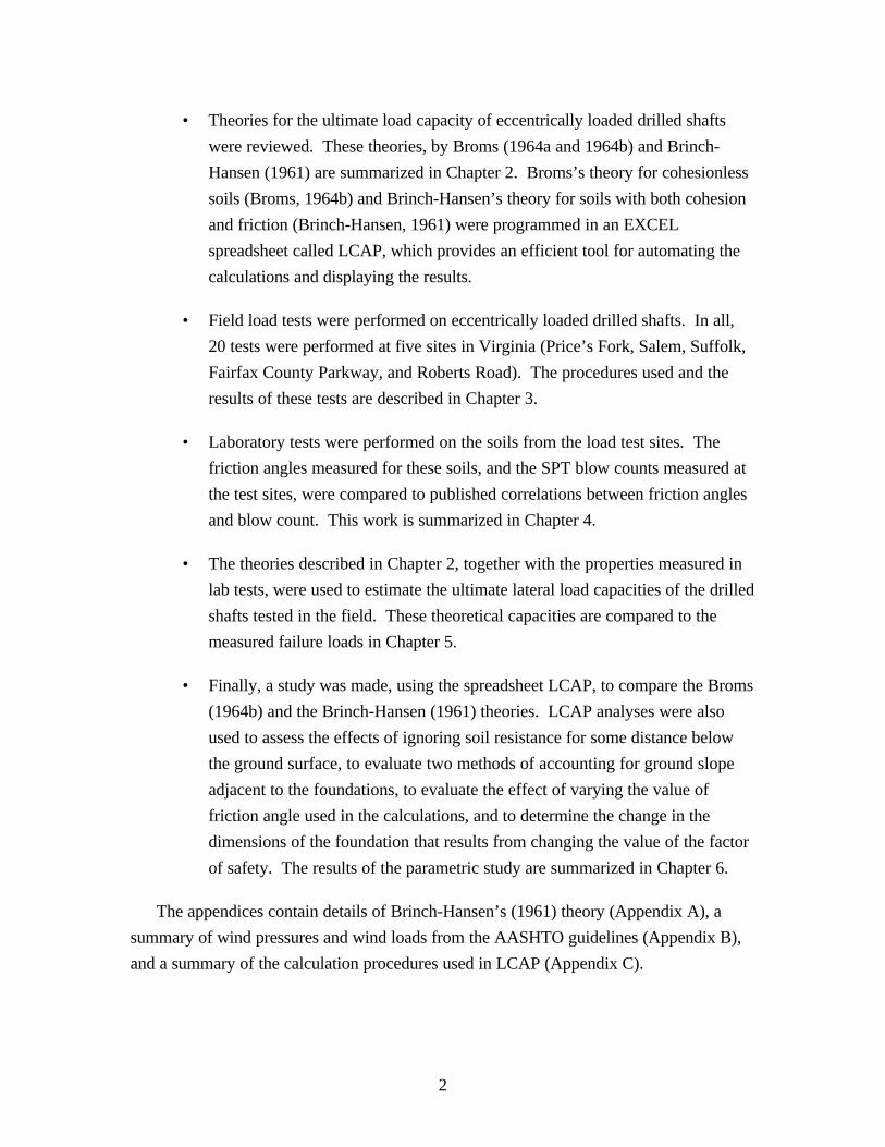
• Theories for the ultimate load capacity of eccentrically loaded drilled shafts

were reviewed. These theories, by Broms (1964a and 1964b) and Brinch-

Hansen (1961) are summarized in Chapter 2. Broms’s theory for cohesionless

soils (Broms, 1964b) and Brinch-Hansen’s theory for soils with both cohesion

and friction (Brinch-Hansen, 1961) were programmed in an EXCEL

spreadsheet called LCAP, which provides an efficient tool for automating the

calculations and displaying the results.

• Field load tests were performed on eccentrically loaded drilled shafts. In all,

20 tests were performed at five sites in Virginia (Price’s Fork, Salem, Suffolk,

Fairfax County Parkway, and Roberts Road). The procedures used and the

results of these tests are described in Chapter 3.

• Laboratory tests were performed on the soils from the load test sites. The

friction angles measured for these soils, and the SPT blow counts measured at

the test sites, were compared to published correlations between friction angles

and blow count. This work is summarized in Chapter 4.

• The theories described in Chapter 2, together with the properties measured in

lab tests, were used to estimate the ultimate lateral load capacities of the drilled

shafts tested in the field. These theoretical capacities are compared to the

measured failure loads in Chapter 5.

• Finally, a study was made, using the spreadsheet LCAP, to compare the Broms

(1964b) and the Brinch-Hansen (1961) theories. LCAP analyses were also

used to assess the effects of ignoring soil resistance for some distance below

the ground surface, to evaluate two methods of accounting for ground slope

adjacent to the foundations, to evaluate the effect of varying the value of

friction angle used in the calculations, and to determine the change in the

dimensions of the foundation that results from changing the value of the factor

of safety. The results of the parametric study are summarized in Chapter 6.

The appendices contain details of Brinch-Hansen’s (1961) theory (Appendix A), a

summary of wind pressures and wind loads from the AASHTO guidelines (Appendix B),

and a summary of the calculation procedures used in LCAP (Appendix C).

3

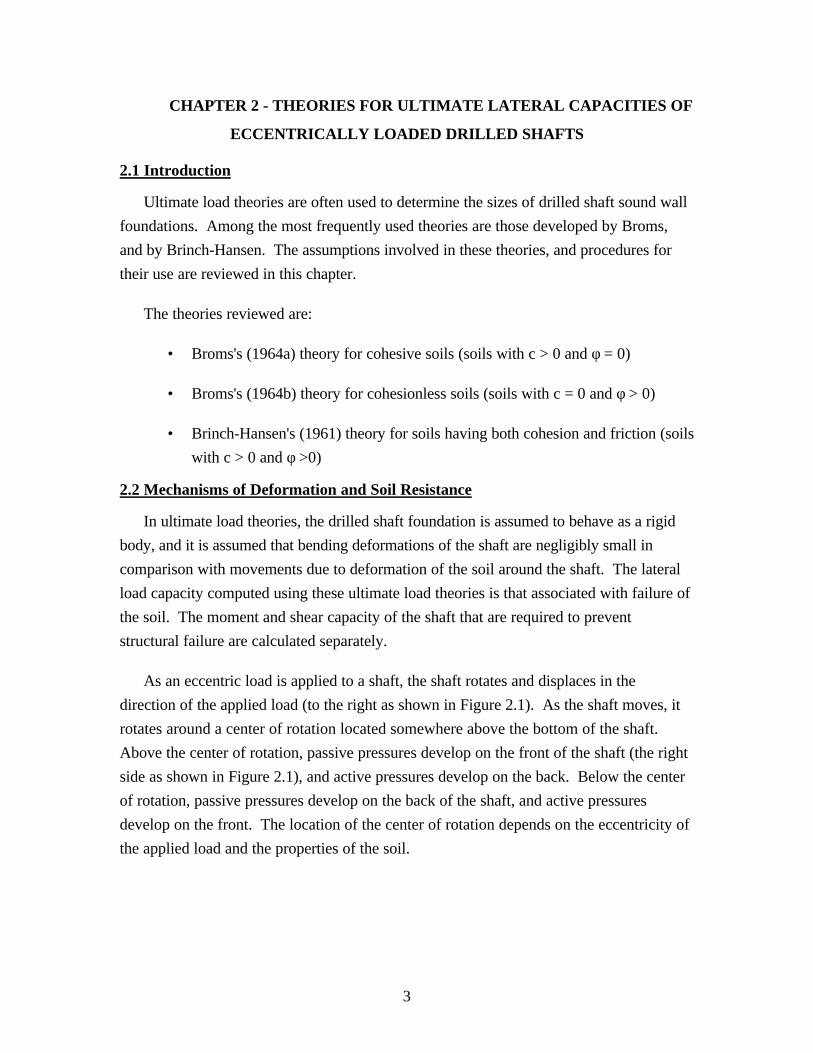
CHAPTER 2 - THEORIES FOR ULTIMATE LATERAL CAPACITIES OF

ECCENTRICALLY LOADED DRILLED SHAFTS

2.1 Introduction

Ultimate load theories are often used to determine the sizes of drilled shaft sound wall

foundations. Among the most frequently used theories are those developed by Broms,

and by Brinch-Hansen. The assumptions involved in these theories, and procedures for

their use are reviewed in this chapter.

The theories reviewed are:

• Broms's (1964a) theory for cohesive soils (soils with c > 0 and φ = 0)

• Broms's (1964b) theory for cohesionless soils (soils with c = 0 and φ > 0)

• Brinch-Hansen's (1961) theory for soils having both cohesion and friction (soils

with c > 0 and φ >0)

2.2 Mechanisms of Deformation and Soil Resistance

In ultimate load theories, the drilled shaft foundation is assumed to behave as a rigid

body, and it is assumed that bending deformations of the shaft are negligibly small in

comparison with movements due to deformation of the soil around the shaft. The lateral

load capacity computed using these ultimate load theories is that associated with failure of

the soil. The moment and shear capacity of the shaft that are required to prevent

structural failure are calculated separately.

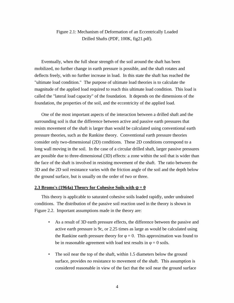
As an eccentric load is applied to a shaft, the shaft rotates and displaces in the

direction of the applied load (to the right as shown in Figure 2.1). As the shaft moves, it

rotates around a center of rotation located somewhere above the bottom of the shaft.

Above the center of rotation, passive pressures develop on the front of the shaft (the right

side as shown in Figure 2.1), and active pressures develop on the back. Below the center

of rotation, passive pressures develop on the back of the shaft, and active pressures

develop on the front. The location of the center of rotation depends on the eccentricity of

the applied load and the properties of the soil.

4

Figure 2.1: Mechanism of Deformation of an Eccentrically Loaded

Drilled Shafts (PDF, 100K, fig21.pdf).

Eventually, when the full shear strength of the soil around the shaft has been

mobilized, no further change in earth pressure is possible, and the shaft rotates and

deflects freely, with no further increase in load. In this state the shaft has reached the

"ultimate load condition." The purpose of ultimate load theories is to calculate the

magnitude of the applied load required to reach this ultimate load condition. This load is

called the "lateral load capacity" of the foundation. It depends on the dimensions of the

foundation, the properties of the soil, and the eccentricity of the applied load.

One of the most important aspects of the interaction between a drilled shaft and the

surrounding soil is that the difference between active and passive earth pressures that

resists movement of the shaft is larger than would be calculated using conventional earth

pressure theories, such as the Rankine theory. Conventional earth pressure theories

consider only two-dimensional (2D) conditions. These 2D conditions correspond to a

long wall moving in the soil. In the case of a circular drilled shaft, larger passive pressures

are possible due to three-dimensional (3D) effects: a zone within the soil that is wider than

the face of the shaft is involved in resisting movement of the shaft. The ratio between the

3D and the 2D soil resistance varies with the friction angle of the soil and the depth below

the ground surface, but is usually on the order of two or three.

2.3 Broms's (1964a) Theory for Cohesive Soils with φφ = 0

This theory is applicable to saturated cohesive soils loaded rapidly, under undrained

conditions. The distribution of the passive soil reaction used in the theory is shown in

Figure 2.2. Important assumptions made in the theory are:

• As a result of 3D earth pressure effects, the difference between the passive and

active earth pressure is 9c, or 2.25 times as large as would be calculated using

the Rankine earth pressure theory for φ = 0. This approximation was found to

be in reasonable agreement with load test results in φ = 0 soils.

• The soil near the top of the shaft, within 1.5 diameters below the ground

surface, provides no resistance to movement of the shaft. This assumption is

considered reasonable in view of the fact that the soil near the ground surface

5

may be weaker than the soil at greater depth due to disturbance during

construction of the shaft and frost action.

Figure 2.2: Broms (1964a) - Assumed Soil Reaction for Cohesive (φ = 0) Material (pdf,

100K, fig22.pdf)

Using the requirements of horizontal equilibrium and moment equilibrium, together

with the distribution of soil resistance shown in Figure 2.2, the following equations can be

derived:

P f 9cD= • (horizontal equilibrium) (2.1)

where:

P = ultimate lateral load, or lateral load capacity of the foundation (force),

f = depth to point of zero shear (units of length),

c = cohesion (units of stress), and

D = diameter of shaft (units of length).

( ) ( )P e 1.5D 0.5f 2.25D 2L 1.5D f c+ + = − − • (moment equilibrium) (2.2)

where:

e = eccentricity of applied load (units of length), and

L = shaft length (units of length).

To compute the magnitude of the lateral load capacity (P), the following procedure

can be used:

1. Use Eq. (2.1) to express f in terms of P.

2. Substitute this expression in Eq. 2.2, and solve for P using an iterative process.

To compute the length required to develop a given value of load capacity (P), the

following procedure can be used:

1. Assume a shaft length (L).

6

2. Follow the procedure above to compute the value of P corresponding to this

shaft length.

3. If the computed value of P is smaller than the given value, increase the value of

L and repeat steps (1) and (2). If the computed value of P is larger than the

given value, reduce the value of L and repeat steps (1) and (2).

2.4 Broms's (1964b) Theory for Cohesionless Soils

This theory is applicable to soils such as sands or gravels, with c = 0. It can also be

used for soils like partly saturated silts or clays that have some cohesion, if the

contribution of cohesion to shaft capacity is neglected.

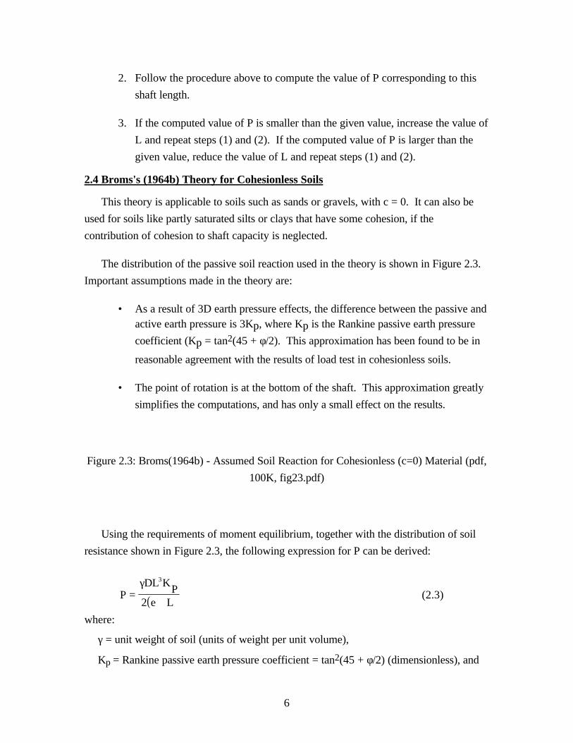
The distribution of the passive soil reaction used in the theory is shown in Figure 2.3.

Important assumptions made in the theory are:

• As a result of 3D earth pressure effects, the difference between the passive andactive earth pressure is 3Kp, where Kp is the Rankine passive earth pressure

coefficient (Kp = tan2(45 + φ/2). This approximation has been found to be in

reasonable agreement with the results of load test in cohesionless soils.

• The point of rotation is at the bottom of the shaft. This approximation greatly

simplifies the computations, and has only a small effect on the results.

Figure 2.3: Broms(1964b) - Assumed Soil Reaction for Cohesionless (c=0) Material (pdf,

100K, fig23.pdf)

Using the requirements of moment equilibrium, together with the distribution of soil

resistance shown in Figure 2.3, the following expression for P can be derived:

( )PDL K

Pe L

3

=+

γ

2(2.3)

where:

γ = unit weight of soil (units of weight per unit volume),

Kp = Rankine passive earth pressure coefficient = tan2(45 + φ/2) (dimensionless), and

7

φ = angle of internal friction (degrees).

The magnitude of the ultimate lateral load can be computed directly using Eq. (2.3).

To compute the length required to develop a given load capacity (P), the following

procedure can be used:

1. Assume a shaft length (L).

2. Use Eq. (2.3) to compute the value of P corresponding to this shaft length.

3. If the computed value of P is smaller than the given value, increase the value of

L and repeat, or, if the computed value of P is larger than the given value,

reduce the value of L and repeat.

2.5 Brinch-Hansen's (1961) Theory for Soils having both Cohesion and Friction

This theory is applicable to soils such as partly saturated silts or clays that have both

cohesion and friction, i. e. c > 0 and φ >0. It can also be used as an alternative to the

Broms theories for frictionless (φ = 0) soils or for cohesionless (c = 0) soils by setting c =

0 or φ = 0 in the equations involved in the theory. This theory has the drawback that it is

much more complex than the Broms theories, but it has the advantage that it can be used

for soils that have both cohesion and friction.

The difference between passive and active earth pressures was expressed by Brinch-

Hansen as:

σ γh

DzKq

cDKc

= + (2.4)

where:

σh = the difference between passive and active earth pressure (units of stress),

z = depth below ground surface (units of length),

Kq = coefficient for the frictional component of net soil resistance under 3D conditions (dimensionless), and

Kc = coefficient for the cohesive component of net soil resistance under 3D conditions (dimensionless).

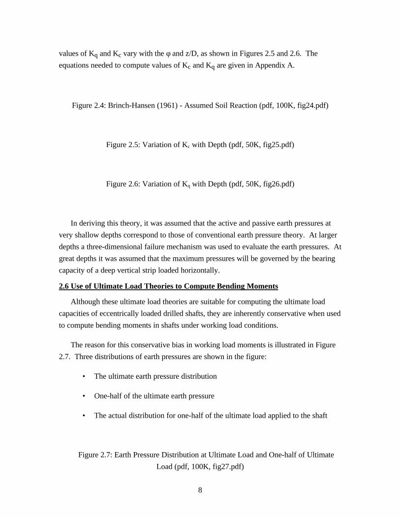
The distribution of the net soil reaction used in the theory is shown in Figure 2.4. The

net soil resistance increases nonlinearly with depth in this relatively complex theory. The

8

values of Kq and Kc vary with the φ and z/D, as shown in Figures 2.5 and 2.6. The

equations needed to compute values of Kc and Kq are given in Appendix A.

Figure 2.4: Brinch-Hansen (1961) - Assumed Soil Reaction (pdf, 100K, fig24.pdf)

Figure 2.5: Variation of Kc with Depth (pdf, 50K, fig25.pdf)

Figure 2.6: Variation of Kq with Depth (pdf, 50K, fig26.pdf)

In deriving this theory, it was assumed that the active and passive earth pressures at

very shallow depths correspond to those of conventional earth pressure theory. At larger

depths a three-dimensional failure mechanism was used to evaluate the earth pressures. At

great depths it was assumed that the maximum pressures will be governed by the bearing

capacity of a deep vertical strip loaded horizontally.

2.6 Use of Ultimate Load Theories to Compute Bending Moments

Although these ultimate load theories are suitable for computing the ultimate load

capacities of eccentrically loaded drilled shafts, they are inherently conservative when used

to compute bending moments in shafts under working load conditions.

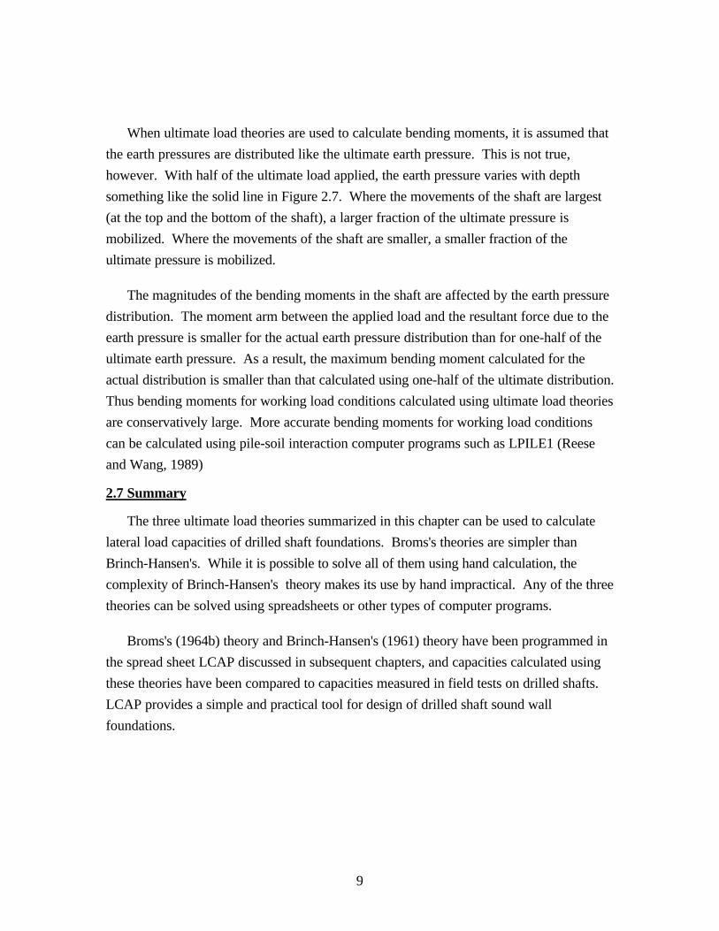
The reason for this conservative bias in working load moments is illustrated in Figure

2.7. Three distributions of earth pressures are shown in the figure:

• The ultimate earth pressure distribution

• One-half of the ultimate earth pressure

• The actual distribution for one-half of the ultimate load applied to the shaft

Figure 2.7: Earth Pressure Distribution at Ultimate Load and One-half of Ultimate

Load (pdf, 100K, fig27.pdf)

9

When ultimate load theories are used to calculate bending moments, it is assumed that

the earth pressures are distributed like the ultimate earth pressure. This is not true,

however. With half of the ultimate load applied, the earth pressure varies with depth

something like the solid line in Figure 2.7. Where the movements of the shaft are largest

(at the top and the bottom of the shaft), a larger fraction of the ultimate pressure is

mobilized. Where the movements of the shaft are smaller, a smaller fraction of the

ultimate pressure is mobilized.

The magnitudes of the bending moments in the shaft are affected by the earth pressure

distribution. The moment arm between the applied load and the resultant force due to the

earth pressure is smaller for the actual earth pressure distribution than for one-half of the

ultimate earth pressure. As a result, the maximum bending moment calculated for the

actual distribution is smaller than that calculated using one-half of the ultimate distribution.

Thus bending moments for working load conditions calculated using ultimate load theories

are conservatively large. More accurate bending moments for working load conditions

can be calculated using pile-soil interaction computer programs such as LPILE1 (Reese

and Wang, 1989)

2.7 Summary

The three ultimate load theories summarized in this chapter can be used to calculate

lateral load capacities of drilled shaft foundations. Broms's theories are simpler than

Brinch-Hansen's. While it is possible to solve all of them using hand calculation, the

complexity of Brinch-Hansen's theory makes its use by hand impractical. Any of the three

theories can be solved using spreadsheets or other types of computer programs.

Broms's (1964b) theory and Brinch-Hansen's (1961) theory have been programmed in

the spread sheet LCAP discussed in subsequent chapters, and capacities calculated using

these theories have been compared to capacities measured in field tests on drilled shafts.

LCAP provides a simple and practical tool for design of drilled shaft sound wall

foundations.

10

CHAPTER 3 - FIELD LOAD TESTS

3.1 Introduction

Field load tests on 20 drilled shafts were performed at five sites in Virginia to assess

the lateral load behavior of drilled shafts in Virginia soils. The soils in many locations

within Virginia are partly saturated, and their strengths are characterized by both cohesion

and friction. The most widely used theories for estimating drilled shaft capacity assume

that the strength of the soil is characterized entirely by cohesion or entirely by friction. It

was therefore considered important to investigate the capacities of drilled shafts in

Virginia soils experimentally, to provide a sound basis for design of drilled shaft sound

wall foundations in the Commonwealth. The methods used in these investigations, and the

results of the load tests, are described in the following sections.

3.2 Test Shaft Construction

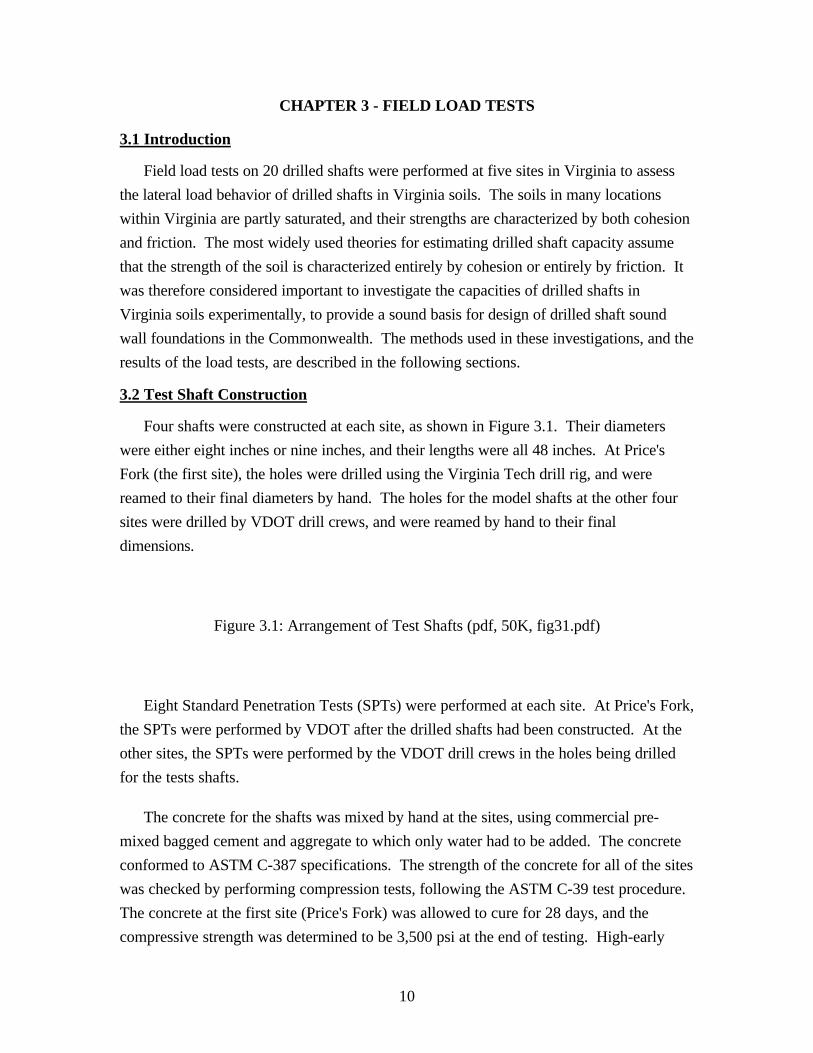
Four shafts were constructed at each site, as shown in Figure 3.1. Their diameters

were either eight inches or nine inches, and their lengths were all 48 inches. At Price's

Fork (the first site), the holes were drilled using the Virginia Tech drill rig, and were

reamed to their final diameters by hand. The holes for the model shafts at the other four

sites were drilled by VDOT drill crews, and were reamed by hand to their final

dimensions.

Figure 3.1: Arrangement of Test Shafts (pdf, 50K, fig31.pdf)

Eight Standard Penetration Tests (SPTs) were performed at each site. At Price's Fork,

the SPTs were performed by VDOT after the drilled shafts had been constructed. At the

other sites, the SPTs were performed by the VDOT drill crews in the holes being drilled

for the tests shafts.

The concrete for the shafts was mixed by hand at the sites, using commercial pre-

mixed bagged cement and aggregate to which only water had to be added. The concrete

conformed to ASTM C-387 specifications. The strength of the concrete for all of the sites

was checked by performing compression tests, following the ASTM C-39 test procedure.

The concrete at the first site (Price's Fork) was allowed to cure for 28 days, and the

compressive strength was determined to be 3,500 psi at the end of testing. High-early

11

strength concrete was used at the other four sites to permit earlier load testing; this

concrete achieved compressive strengths in excess of 3,500 psi at the time of testing.

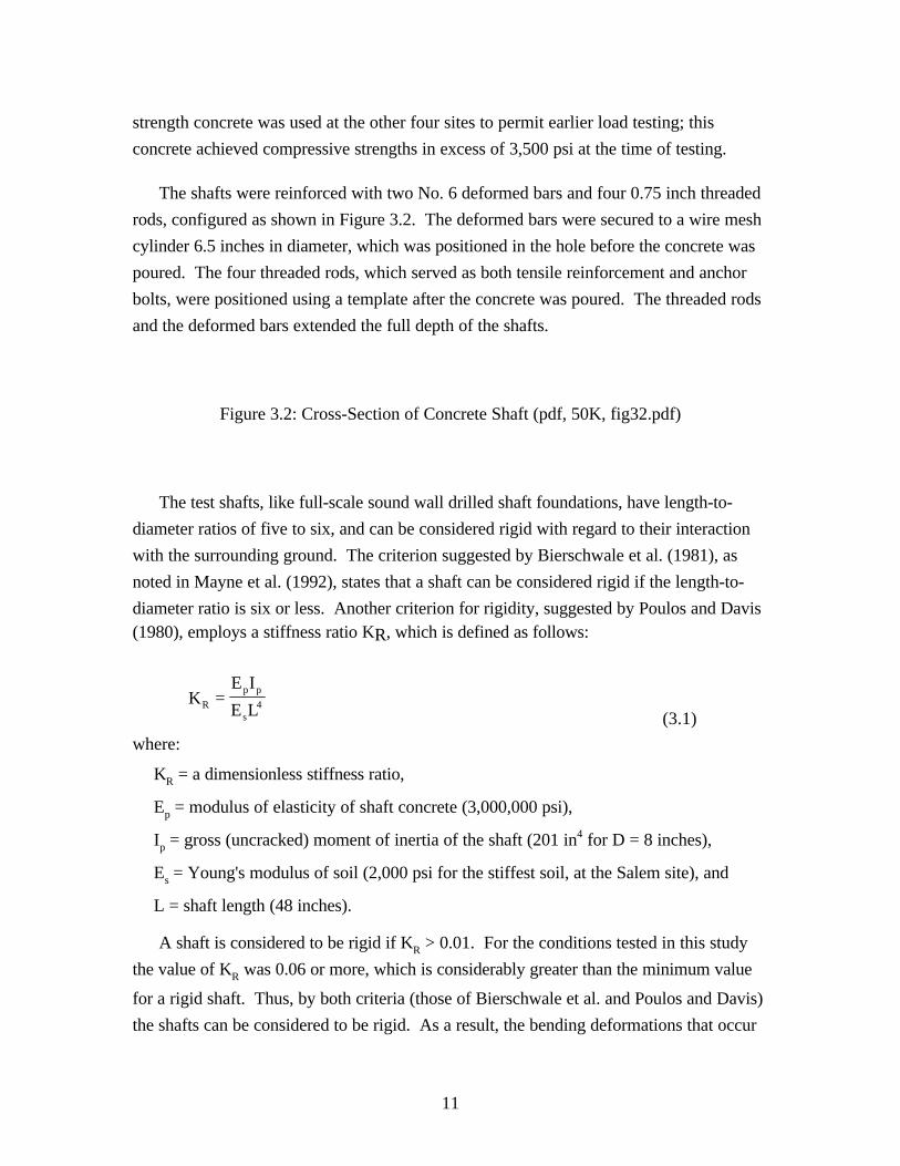
The shafts were reinforced with two No. 6 deformed bars and four 0.75 inch threaded

rods, configured as shown in Figure 3.2. The deformed bars were secured to a wire mesh

cylinder 6.5 inches in diameter, which was positioned in the hole before the concrete was

poured. The four threaded rods, which served as both tensile reinforcement and anchor

bolts, were positioned using a template after the concrete was poured. The threaded rods

and the deformed bars extended the full depth of the shafts.

Figure 3.2: Cross-Section of Concrete Shaft (pdf, 50K, fig32.pdf)

The test shafts, like full-scale sound wall drilled shaft foundations, have length-to-

diameter ratios of five to six, and can be considered rigid with regard to their interaction

with the surrounding ground. The criterion suggested by Bierschwale et al. (1981), as

noted in Mayne et al. (1992), states that a shaft can be considered rigid if the length-to-

diameter ratio is six or less. Another criterion for rigidity, suggested by Poulos and Davis(1980), employs a stiffness ratio KR, which is defined as follows:

K =E I

E LR

p p

s4

(3.1)

where:

KR = a dimensionless stiffness ratio,

Ep = modulus of elasticity of shaft concrete (3,000,000 psi),

Ip = gross (uncracked) moment of inertia of the shaft (201 in4 for D = 8 inches),

Es = Young's modulus of soil (2,000 psi for the stiffest soil, at the Salem site), and

L = shaft length (48 inches).

A shaft is considered to be rigid if KR > 0.01. For the conditions tested in this study

the value of KR was 0.06 or more, which is considerably greater than the minimum value

for a rigid shaft. Thus, by both criteria (those of Bierschwale et al. and Poulos and Davis)

the shafts can be considered to be rigid. As a result, the bending deformations that occur

12

when they are loaded are not appreciable compared to the deflections and rotations

resulting from the deformation of the surrounding soil.

3.3 Loading Equipment

The loading equipment used for the tests was developed with these objectives in mind:

• Easy setup and disassembly,

• Multiple tests at each site, and

• Efficient and practical load reaction system.

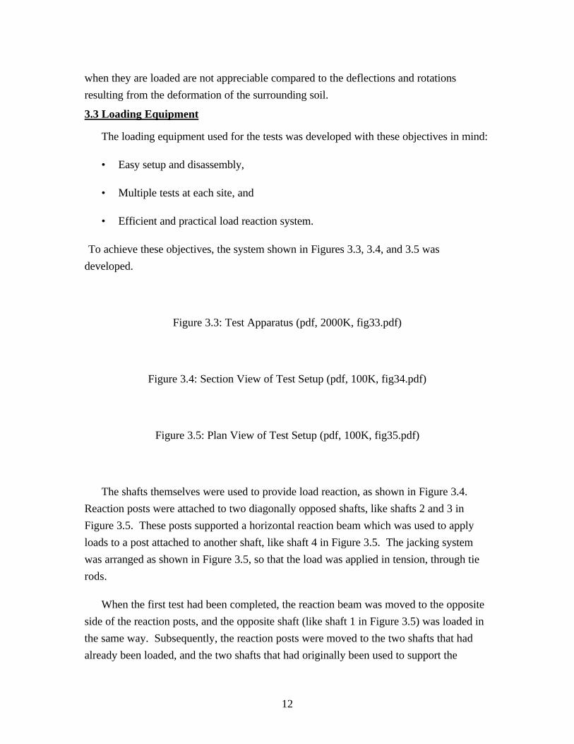
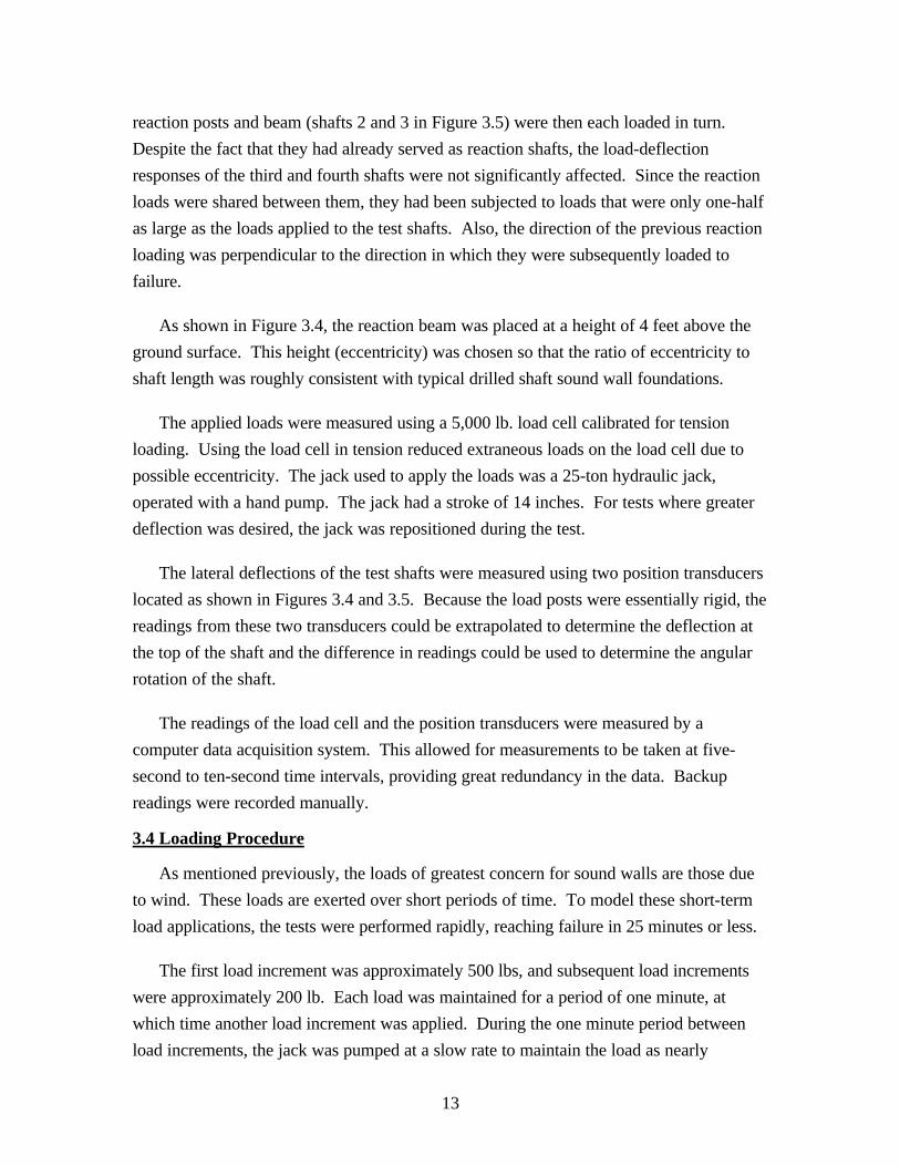
To achieve these objectives, the system shown in Figures 3.3, 3.4, and 3.5 was

developed.

Figure 3.3: Test Apparatus (pdf, 2000K, fig33.pdf)

Figure 3.4: Section View of Test Setup (pdf, 100K, fig34.pdf)

Figure 3.5: Plan View of Test Setup (pdf, 100K, fig35.pdf)

The shafts themselves were used to provide load reaction, as shown in Figure 3.4.

Reaction posts were attached to two diagonally opposed shafts, like shafts 2 and 3 in

Figure 3.5. These posts supported a horizontal reaction beam which was used to apply

loads to a post attached to another shaft, like shaft 4 in Figure 3.5. The jacking system

was arranged as shown in Figure 3.5, so that the load was applied in tension, through tie

rods.

When the first test had been completed, the reaction beam was moved to the opposite

side of the reaction posts, and the opposite shaft (like shaft 1 in Figure 3.5) was loaded in

the same way. Subsequently, the reaction posts were moved to the two shafts that had

already been loaded, and the two shafts that had originally been used to support the

13

reaction posts and beam (shafts 2 and 3 in Figure 3.5) were then each loaded in turn.

Despite the fact that they had already served as reaction shafts, the load-deflection

responses of the third and fourth shafts were not significantly affected. Since the reaction

loads were shared between them, they had been subjected to loads that were only one-half

as large as the loads applied to the test shafts. Also, the direction of the previous reaction

loading was perpendicular to the direction in which they were subsequently loaded to

failure.

As shown in Figure 3.4, the reaction beam was placed at a height of 4 feet above the

ground surface. This height (eccentricity) was chosen so that the ratio of eccentricity to

shaft length was roughly consistent with typical drilled shaft sound wall foundations.

The applied loads were measured using a 5,000 lb. load cell calibrated for tension

loading. Using the load cell in tension reduced extraneous loads on the load cell due to

possible eccentricity. The jack used to apply the loads was a 25-ton hydraulic jack,

operated with a hand pump. The jack had a stroke of 14 inches. For tests where greater

deflection was desired, the jack was repositioned during the test.

The lateral deflections of the test shafts were measured using two position transducers

located as shown in Figures 3.4 and 3.5. Because the load posts were essentially rigid, the

readings from these two transducers could be extrapolated to determine the deflection at

the top of the shaft and the difference in readings could be used to determine the angular

rotation of the shaft.

The readings of the load cell and the position transducers were measured by a

computer data acquisition system. This allowed for measurements to be taken at five-

second to ten-second time intervals, providing great redundancy in the data. Backup

readings were recorded manually.

3.4 Loading Procedure

As mentioned previously, the loads of greatest concern for sound walls are those due

to wind. These loads are exerted over short periods of time. To model these short-term

load applications, the tests were performed rapidly, reaching failure in 25 minutes or less.

The first load increment was approximately 500 lbs, and subsequent load increments

were approximately 200 lb. Each load was maintained for a period of one minute, at

which time another load increment was applied. During the one minute period between

load increments, the jack was pumped at a slow rate to maintain the load as nearly

14

constant as possible. As can be seen in Figure 3.6, this test procedure resulted in a series

of nearly horizontal load plateaus. Examination of the data in Figure 3.6 shows where

each load was maintained, and the movement that occurred during the one minute time

period. As expected, the amount of deflection over the one minute time period increased

as the level of loading increased.

Figure 3.6: Typical Load Deflection Curve (pdf, 50K, fig36.pdf)

The loading sequence was continued until the load could not be increased. This

occurred in a dramatic manner in some cases, where brittle failure occurred. In some

tests, less dramatic ductile failure occurred. In these ductile failure cases, the load could

be maintained but not increased. Once failure was reached, loading was discontinued, to

avoid additional deflection. Thus, especially for the cases where brittle failure occurred, it

is unclear what shape the load deflection curve would have exhibited if further deflections

had been imposed. It was clear, based on observations made during testing, that failure

occurred due to reaching the ultimate capacity of the soil around the shafts. The only

exception was at Price's Fork, where there was some crushing of the concrete beneath the

base plate on the first shaft constructed, due to the poor quality of the concrete at the top

of the shaft.

3.5 Test Results

A variety of soil conditions were encountered at the five sites. The properties of the

soils are discussed in Chapter 4. The load deflection results from the five sites are shown

in Figure 3.7 through 3.11. The deflection values shown on the horizontal axes are those

at the tops of the shafts (at ground level). The average ultimate loads for the five sites are

listed in Table 3.1. The Unified Soil classifications, the average degree of saturation(S),

and the Standard Penetration Test blow count (N) are shown in the figures. The values of

(N1)60 are values of N corrected for overburden pressure and hammer energy, as explained

in Chapter 4.

Figure 3.7: Prices Fork Load Deflection Curves (pdf, 50K, fig37.pdf)

15

Figure 3.8: Salem Load Deflection Curves (pdf, 50K, fig38.pdf)

Figure 3.9: Suffolk Load Deflection Curves (pdf, 50K, fig39.pdf)

Figure 3.10: Fairfax County Parkway Load Deflection Curves (pdf, 50K, fig310.pdf)

Figure 3.11: Roberts Road Load Deflection Curves (pdf, 50K, fig311.pdf)

The results of Test No. 1 at Price’s Fork, in which poor quality concrete affected the

behavior, were not used in determining the average ultimate load for Price's Fork that is

shown in Table 3.1.

The shafts at the Salem site all exhibited brittle soil failure, with the loads dropping off

rapidly after the maximum load was reached. As noted previously, no attempt was made

to maintain the load after failure when brittle failure occurred, to avoid unnecessarily large

deflections.

Test shaft No. 4 at Suffolk (Figure 3.9) was subjected to two unload-reload cycles.

The first unloading was at approximately 45% of the ultimate load and the second cycle

was at about 62% of the ultimate load. These cycles did not appear to affect the ultimate

load.

Test shaft No. 4 at Fairfax County Parkway (Figure 3.10) was also subjected to two

unload-reload cycles. As at Suffolk, these load cycles did not appear to affect the failure

load for the test.

The average deflection measured at the Roberts Road site was the smallest for any

site. The deflections at failure in Tests No. 1 and No. 3 were only about 1.0 inch. The

load deflection curves showed dramatic drop-off, characteristic of brittle failure.

16

Two unload-load cycles were performed during test No. 4 at Roberts Road (Figure

3.11), at approximately 40% and 64% of the ultimate load. The ultimate load achieved

during this test was slightly lower than the ultimate for the other three tests, but the

difference was not great.

3.6 Summary

As would be expected because of the variations in soil conditions at the five sites, the

maximum loads and the magnitudes of deflection varied somewhat from one site to

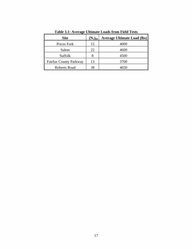
another. The values of the average ultimate load for each site are shown in Table 3.1, and

average load-deflection curves for the five sites are shown in Figure 3.12. The load

deflection curves shown in Figure 3.12 are average curves for the four tests performed at

each site.

Figure 3.12: Summary of Field Load Tests (pdf, 50K, fig312.pdf)

The values of ultimate load at the Roberts Road site were the highest and the

deflections were the smallest of any of the five sites. As discussed in Chapter 4, the soil at

Roberts Road was non-plastic, and had the highest corrected blow count of any site,(N1)60 = 38. The smallest values of ultimate load, and the largest values of deflection,

were measured at the Fairfax County Parkway site. The soil at this site contained highly

plastic clay and silt (CL to CH), and had the second lowest corrected blow count of anysite, (N1)60 = 13.

The load-deflection curves for the Salem site and the Roberts Road site exhibited the

most dramatic drop-off of load after peak load was reached. The Salem soil contained siltand clay of low plasticity, and had a corrected blow count (N1)60 = 22.

The load and unload cycles performed at the Suffolk, Fairfax County Parkway, and

Roberts Road Site showed that two cycles had little effect on the measured values of

ultimate load. However, each load cycle did induce added deformations in the range of

0.1 inches at about 40% of the ultimate load. Since only two cycles of loading were

performed, the behavior under additional cycles cannot be generalized from this data, and

the effects of cyclic load variations needs further study.

17

Table 3.1: Average Ultimate Loads from Field Tests

Site (N1)60 Average Ultimate Load (lbs)

Prices Fork 15 4000

Salem 22 4600

Suffolk 8 4500

Fairfax County Parkway 13 3700

Roberts Road 38 4650

18

CHAPTER 4 - SOIL PROPERTIES

4.1 Introduction

Field and laboratory tests were performed to assess the properties of the soils at the

sites where the load tests were performed. Standard Penetration Tests (SPT) were

performed in the field. Index tests and triaxial compression tests were performed in the

laboratory.

4.2 Standard Penetration Tests

The SPT tests were performed according to ASTM D-1586. A total of eight tests

were performed at each site, two tests in each of four boreholes. For all sites except

Prices Fork, the SPT’s were performed in the boreholes in which test shafts were later

constructed, as shown Figures 4.1 through 4.5. Within each borehole, SPT values were

determined at two depths.

Figure 4.1: Site Plan, Prices Fork (pdf, 50K, fig41.pdf)

Figure 4.2: Site Plan, Salem (pdf, 50K, fig42.pdf)

Figure 4.3: Site Plan, Suffolk (pdf, 50K, fig43.pdf)

Figure 4.4: Site Plan, Fairfax County Parkway (pdf, 50K, fig44.pdf)

Figure 4.5: Site Plan, Roberts Road (pdf, 50K, fig45.pdf)

The type of hammer and the release mechanism varied from site to site. These

variations were taken into account by correcting the SPT N-values for hammer energy.

The measured N-values were also corrected for the effect of overburden pressure. The

19

corrected N-values are denoted as values of (N1)60, which corresponds to a standardized

overburden pressure of one ton per square ft., and a standardized hammer energy equal to

60 percent of the theoretical value. Additional corrections were made to account for the

test procedures used with respect to borehole diameter, sampler liners, and rod length.

The following equation was used to account for these effects:

(N N C C C C C1 Field N E R B S)60 = (3.1)

where:

(N1)60 = N-value corrected to 60% of the theoretical energy and 1.0 t/ft2 overburdenpressure,

NField = number of blows per foot measured in the field,

CN = overburden pressure correction factor,

CNvo

=

0 77

20. log

'σ(Peck, Hansen, and Thornburn, 1974),

σvo’ = effective overburden pressure (≥0.25 t/ft2)

CE = hammer energy correction factor,

C =(E.R.)

60E (Skempton 1986),

CR = correction factor for rod length (=0.75 for rod length, 4 meters),

CB = borehole diameter correction factor (=1.15 for 8 in diameter hole),

CS = sampler correction factor (=1.2 since no liners were used),

σvo’ = effective vertical overburden pressure (≥ 0.25t/ft2), and

E.R. = energy ratio (%) for specific SPT hammer.

Hammer energies were not measured during the tests. To account for hammer energy

effects the following energy ratios, recommended by Kovacs (1994), were used for the

hammers and release mechanisms used in tests:

• E.R. = 60 for safety hammer and cathead release mechanism, and

• E.R. = 90 for automatic trip safety hammer.

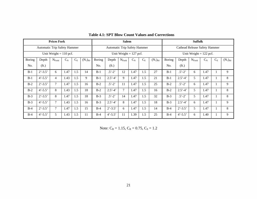
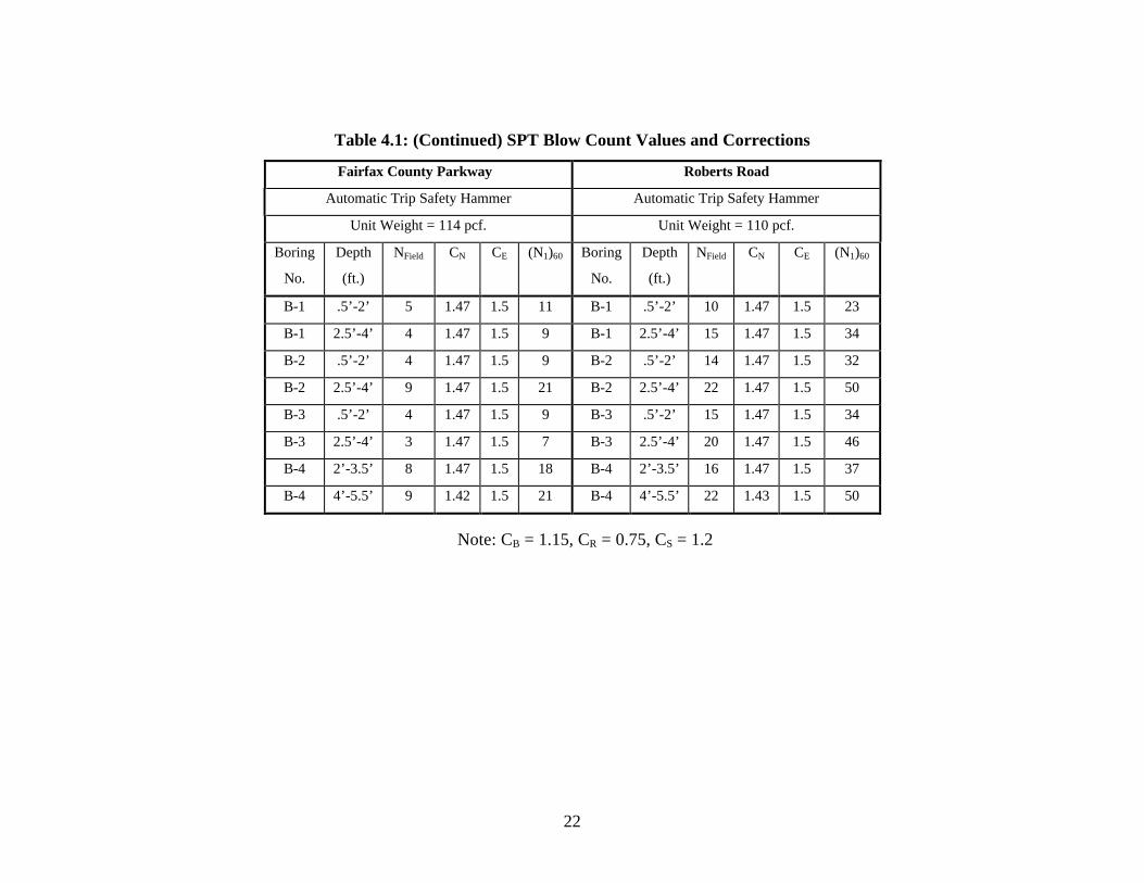
The blow count values from the SPTs are summarized in Table 4.1. Also shown in

Table 4.1 are the hammer types and release mechanisms, the unit weights of the soils, and

the resulting correction factors for hammer energy and overburden pressure used for each

20

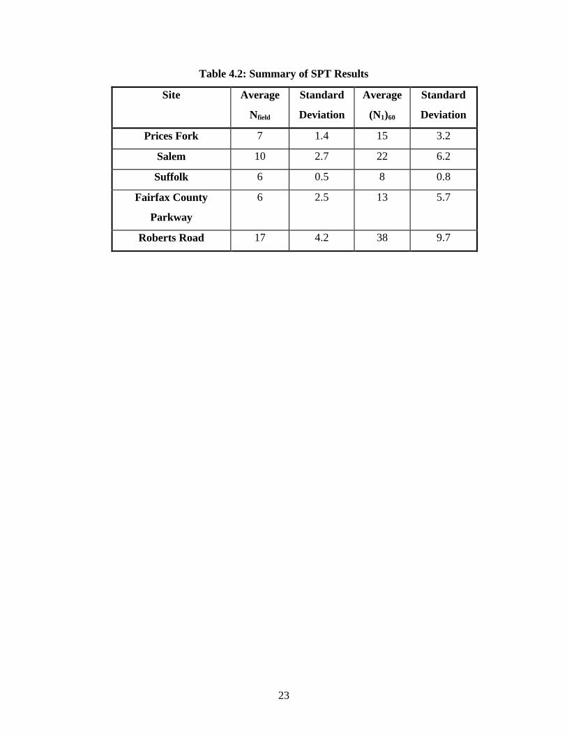
site in determining (N1)60 values. The average values of Nfield, (N1)60, and standard

deviations of these quantities for each site are shown in Table 4.2.

4.3 Summary of SPT Results

The values of Nfield = 17 and (N1)60 = 38 for Roberts Road were the highest of the five

sites. Both Suffolk and Fairfax County Parkway had Nfield = 6, the lowest for any of the

sites. Due to differences in the release mechanisms of the SPT equipment used at these

sites, the values of (N1)60 were 8 for Suffolk and 13 for Fairfax County Parkway.

The values of Nfield and (N1)60 measures at Roberts Road varied more widely than at

the other sites. The values of Nfield ranged from 10 to 22 and the values of (N1)60 ranged

from 23 to 50. The smallest variation in blow count was found at Suffolk, where the

values of Nfield varied from 5 to 6, and the (N1)60 varied from 8 to 9.

Examining the field blow count values in comparison to the corrected blow count

values, it is evident that the corrections for overburden pressure and hammer energy are

significant. The overburden corrections are greater than unity and are quite large due to

the shallow depths at which the tests were performed. Since in most cases drilled shaft

sound wall foundations will be constructed at shallow depths (although not as shallow as

the test shafts) the overburden pressure effect can be expected to be quite significant.

4.4 Classification Tests

The split spoon samples from the Standard Penetration Tests were used for Atterberg

Limit and grain size analysis tests. The ASTM D-4318 and ASTM D-422 test procedures

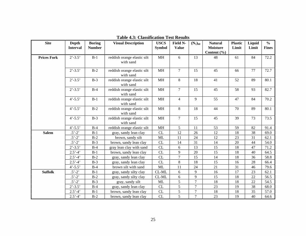
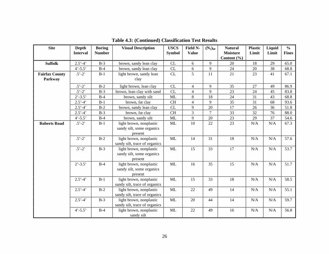
respectively were followed in performing the tests. Using the results of these tests, the

soils were classified according to the Unified Soil Classification System described in

ASTM D-2487. The results of the classification tests are summarized in Table 4.3, and

the results of the Atterberg Limits tests are shown in Figure 4.6. Individual characteristics

of the soils at each site are described below.

Figure 4.6: Summary of Atterberg limits (pdf, 50K, fig46.pdf)

21

Table 4.1: SPT Blow Count Values and Corrections

Prices Fork Salem Suffolk

Automatic Trip Safety Hammer Automatic Trip Safety Hammer Cathead Release Safety Hammer

Unit Weight = 110 pcf. Unit Weight = 127 pcf. Unit Weight = 122 pcf.

Boring

No.

Depth

(ft.)

NField CN CE (N1)60 Boring

No.

Depth

(ft.)

NField CN CE (N1)60 Boring

No.

Depth

(ft.)

NField CN CE (N1)60

B-1 2’-3.5’ 6 1.47 1.5 14 B-1 .5’-2’ 12 1.47 1.5 27 B-1 .5’-2’ 6 1.47 1 9

B-1 4’-5.5’ 4 1.43 1.5 9 B-1 2.5’-4’ 9 1.47 1.5 21 B-1 2.5’-4’ 5 1.47 1 8

B-2 2’-3.5’ 7 1.47 1.5 16 B-2 .5’-2’ 11 1.47 1.5 25 B-2 .5’-2’ 6 1.47 1 9

B-2 4’-5.5’ 8 1.43 1.5 18 B-2 2.5’-4’ 7 1.47 1.5 16 B-2 2.5’-4’ 5 1.47 1 8

B-3 2’-3.5’ 8 1.47 1.5 18 B-3 .5’-2’ 14 1.47 1.5 32 B-3 .5’-2’ 5 1.47 1 8

B-3 4’-5.5’ 7 1.43 1.5 16 B-3 2.5’-4’ 8 1.47 1.5 18 B-3 2.5’-4’ 6 1.47 1 9

B-4 2’-3.5’ 7 1.47 1.5 15 B-4 2’-3.5’ 6 1.47 1.5 14 B-4 2’-3.5’ 5 1.47 1 8

B-4 4’-5.5’ 5 1.43 1.5 11 B-4 4’-5.5’ 11 1.39 1.5 25 B-4 4’-5.5’ 6 1.40 1 9

Note: CB = 1.15, CR = 0.75, CS = 1.2

22

Table 4.1: (Continued) SPT Blow Count Values and Corrections

Fairfax County Parkway Roberts Road

Automatic Trip Safety Hammer Automatic Trip Safety Hammer

Unit Weight = 114 pcf. Unit Weight = 110 pcf.

Boring

No.

Depth

(ft.)

NField CN CE (N1)60 Boring

No.

Depth

(ft.)

NField CN CE (N1)60

B-1 .5’-2’ 5 1.47 1.5 11 B-1 .5’-2’ 10 1.47 1.5 23

B-1 2.5’-4’ 4 1.47 1.5 9 B-1 2.5’-4’ 15 1.47 1.5 34

B-2 .5’-2’ 4 1.47 1.5 9 B-2 .5’-2’ 14 1.47 1.5 32

B-2 2.5’-4’ 9 1.47 1.5 21 B-2 2.5’-4’ 22 1.47 1.5 50

B-3 .5’-2’ 4 1.47 1.5 9 B-3 .5’-2’ 15 1.47 1.5 34

B-3 2.5’-4’ 3 1.47 1.5 7 B-3 2.5’-4’ 20 1.47 1.5 46

B-4 2’-3.5’ 8 1.47 1.5 18 B-4 2’-3.5’ 16 1.47 1.5 37

B-4 4’-5.5’ 9 1.42 1.5 21 B-4 4’-5.5’ 22 1.43 1.5 50

Note: CB = 1.15, CR = 0.75, CS = 1.2

23

Table 4.2: Summary of SPT Results

Site Average

Nfield

Standard

Deviation

Average

(N1)60

Standard

Deviation

Prices Fork 7 1.4 15 3.2

Salem 10 2.7 22 6.2

Suffolk 6 0.5 8 0.8

Fairfax County

Parkway

6 2.5 13 5.7

Roberts Road 17 4.2 38 9.7

24

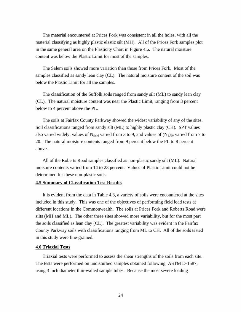
The material encountered at Prices Fork was consistent in all the holes, with all the

material classifying as highly plastic elastic silt (MH). All of the Prices Fork samples plot

in the same general area on the Plasticity Chart in Figure 4.6. The natural moisture

content was below the Plastic Limit for most of the samples.

The Salem soils showed more variation than those from Prices Fork. Most of the

samples classified as sandy lean clay (CL). The natural moisture content of the soil was

below the Plastic Limit for all the samples.

The classification of the Suffolk soils ranged from sandy silt (ML) to sandy lean clay

(CL). The natural moisture content was near the Plastic Limit, ranging from 3 percent

below to 4 percent above the PL.

The soils at Fairfax County Parkway showed the widest variability of any of the sites.

Soil classifications ranged from sandy silt (ML) to highly plastic clay (CH). SPT values

also varied widely: values of Nfield varied from 3 to 9, and values of (N1)60 varied from 7 to

20. The natural moisture contents ranged from 9 percent below the PL to 8 percent

above.

All of the Roberts Road samples classified as non-plastic sandy silt (ML). Natural

moisture contents varied from 14 to 23 percent. Values of Plastic Limit could not be

determined for these non-plastic soils.

4.5 Summary of Classification Test Results

It is evident from the data in Table 4.3, a variety of soils were encountered at the sites

included in this study. This was one of the objectives of performing field load tests at

different locations in the Commonwealth. The soils at Prices Fork and Roberts Road were

silts (MH and ML). The other three sites showed more variability, but for the most part

the soils classified as lean clay (CL). The greatest variability was evident in the Fairfax

County Parkway soils with classifications ranging from ML to CH. All of the soils tested

in this study were fine-grained.

4.6 Triaxial Tests

Triaxial tests were performed to assess the shear strengths of the soils from each site.

The tests were performed on undisturbed samples obtained following ASTM D-1587,

using 3 inch diameter thin-walled sample tubes. Because the most severe loading

25

Table 4.3: Classification Test ResultsSite Depth

IntervalBoring

NumberVisual Description USCS

SymbolField N-

Value(N1)60 Natural

MoistureContent (%)

PlasticLimit

LiquidLimit

%Fines

Prices Fork 2’-3.5’ B-1 reddish orange elastic siltwith sand

MH 6 13 48 61 84 72.2

2’-3.5’ B-2 reddish orange elastic siltwith sand

MH 7 15 45 66 77 72.7

2’-3.5’ B-3 reddish orange elastic siltwith sand

MH 8 18 41 52 89 80.1

2’-3.5’ B-4 reddish orange elastic siltwith sand

MH 7 15 45 58 93 82.7

4’-5.5’ B-1 reddish orange elastic siltwith sand

MH 4 9 55 47 84 70.2

4’-5.5’ B-2 reddish orange elastic siltwith sand

MH 8 18 44 70 89 80.1

4’-5.5’ B-3 reddish orange elastic siltwith sand

MH 7 15 45 39 73 73.5

4’-5.5’ B-4 reddish orange elastic silt MH 5 11 53 59 82 91.4Salem .5’-2’ B-1 gray, sandy lean clay CL 12 26 12 18 38 69.0

.5’-2’ B-2 brown, sandy silt ML 11 24 12 23 31 62.1

.5’-2’ B-3 brown, sandy lean clay CL 14 31 14 20 44 54.02’-3.5’ B-4 gray lean clay with sand CL 6 13 15 18 47 71.22.5’-4’ B-1 brown, sandy lean clay CL 9 20 15 18 40 64.52.5’-4’ B-2 gray, sandy lean clay CL 7 15 14 18 36 58.82.5’-4’ B-3 gray, sandy lean clay CL 8 18 15 16 28 66.44’-5.5’ B-4 brown silt with sand ML 11 24 21 31 46 79.6

Suffolk .5’-2’ B-1 gray, sandy silty clay CL-ML 6 9 16 17 23 62.1.5’-2’ B-2 gray, sandy silty clay CL-ML 6 9 15 18 22 56.5.5’-2’ B-3 gray, sandy silt ML 5 7 18 18 22 54.52’-3.5’ B-4 gray, sandy lean clay CL 5 7 23 19 38 68.02.5’-4’ B-1 brown, sandy lean clay CL 5 7 18 18 35 57.02.5’-4’ B-2 brown, sandy lean clay CL 5 7 23 19 40 64.6

26

Table 4.3: (Continued) Classification Test Results

Site DepthInterval

BoringNumber

Visual Description USCSSymbol

Field N-Value

(N1)60 NaturalMoisture

Content (%)

PlasticLimit

LiquidLimit

%Fines

Suffolk 2.5’-4’ B-3 brown, sandy lean clay CL 6 9 20 18 29 65.04’-5.5’ B-4 brown, sandy lean clay CL 6 9 24 20 38 68.8

Fairfax CountyParkway

.5’-2’ B-1 light brown, sandy leanclay

CL 5 11 21 23 41 67.1

.5’-2’ B-2 light brown, lean clay CL 4 9 35 27 49 86.9

.5’-2’ B-3 brown, lean clay with sand CL 4 9 23 24 45 83.82’-3.5’ B-4 brown, sandy silt ML 8 18 24 31 43 68.82.5’-4’ B-1 brown, fat clay CH 4 9 35 31 68 93.62.5’-4’ B-2 brown, sandy lean clay CL 9 20 17 26 36 51.82.5’-4’ B-3 brown, fat clay CH 3 7 33 32 76 88.04’-5.5’ B-4 brown, sandy silt ML 9 20 23 29 37 54.6

Roberts Road .5’-2’ B-1 light brown, nonplasticsandy silt, some organics

present

ML 10 22 23 N/A N/A 67.3

.5’-2’ B-2 light brown, nonplasticsandy silt, trace of organics

ML 14 31 18 N/A N/A 57.6

.5’-2’ B-3 light brown, nonplasticsandy silt, some organics

present

ML 15 33 17 N/A N/A 53.7

2’-3.5’ B-4 light brown, nonplasticsandy silt, some organics

present

ML 16 35 15 N/A N/A 51.7

2.5’-4’ B-1 light brown, nonplasticsandy silt, trace of organics

ML 15 33 18 N/A N/A 58.5

2.5’-4’ B-2 light brown, nonplasticsandy silt, trace of organics

ML 22 49 14 N/A N/A 55.1

2.5’-4’ B-3 light brown, nonplasticsandy silt, trace of organics

ML 20 44 14 N/A N/A 59.7

4’-5.5’ B-4 light brown, nonplasticsandy silt

ML 22 49 16 N/A N/A 56.8

27

conditions for sound wall foundations are short term wind loads, unconsolidated-

undrained triaxial tests were performed on the samples following ASTM D-2850. A

loading rate of 1% axial strain per minute was used in performing the tests. This led to

testing times of approximately 20 minutes, because the tests were continued to 20% axial

strain.

The confining pressures used during the tests were in the same range as the estimated

overburden pressures at the sample depths.

Peak deviator stress was used as the failure criterion if the peak was reached at 10%

axial strain or less. If the peak did not occur below 10% axial strain, the deviator stress at

10% axial strain was used as the failure criterion.

Deviator stress versus axial strain curves for the tests are shown in Figures 4.7a, 4.8a,

4.9a, 4.10a, and 4.11a. The strength envelopes derived from the test results are shown in

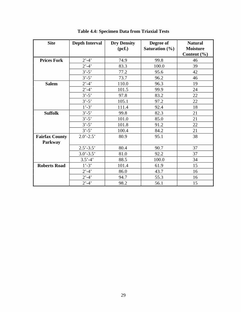
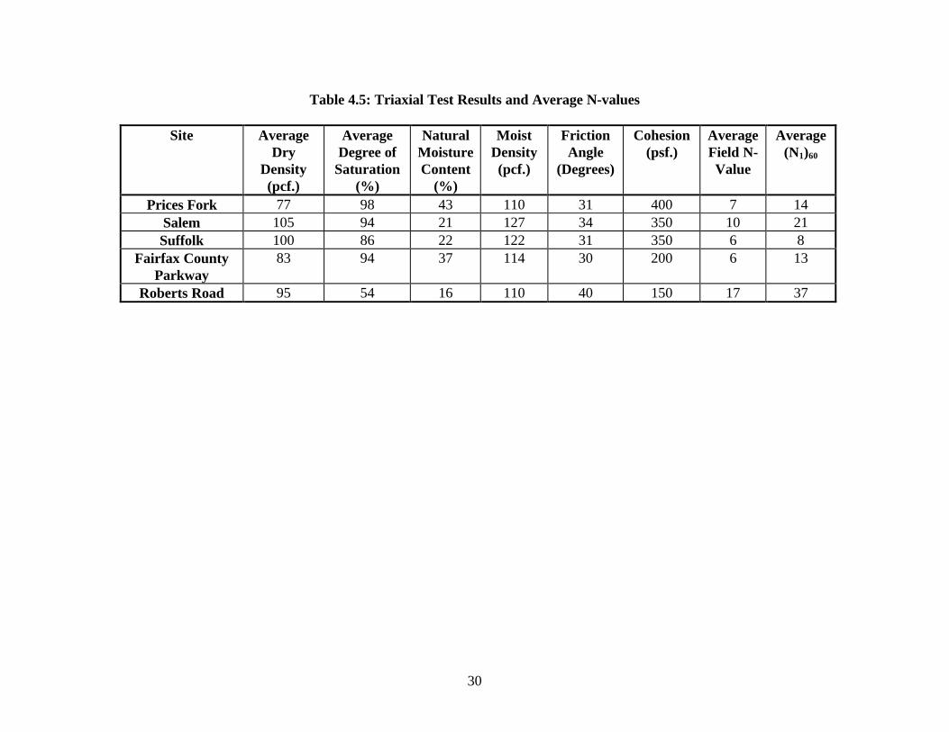
Figures 4.7b, 4.8b, 4.9b, 4.10b, and 4.11b. The depth, dry density, degree of saturation,

and natural moisture content for each specimen are summarized in Table 4.4, and the

strength properties and material properties are given in Table 4.5.

Figure 4.7a: Prices Fork, Deviator Stress vs. Axial Strain Curves (pdf, 50K, fig47a.pdf)

Figure 4.7b: Prices Fork, Strength Envelope (pdf, 50K, fig47b.pdf)

Figure 4.8a: Salem, Deviator Stress vs. Axial Strain Curves (pdf, 50K, fig48a.pdf)

Figure 4.8b: Salem, Strength Envelope (pdf, 50K, fig48b.pdf)

Figure 4.9a: Suffolk, Deviator Stress vs. Axial Strain Curves (pdf, 50K, fig49a.pdf)

28

Figure 4.9b: Suffolk, Strength Envelope (pdf, 50K, fig49b.pdf)

Figure 4.10a: Fairfax County Parkway, Deviator Stress vs. Axial Strain Curves (pdf, 50K,

fig410a.pdf)

Figure 4.10b: Fairfax County Parkway, Strength Envelope (pdf, 50K, fig410b.pdf)

Figure 4.11a: Roberts Road, Deviator Stress vs. Axial Strain Curves (pdf, 50K,

fig411a.pdf)

Figure 4.11b: Roberts Road, Strength Envelope (pdf, 50K, fig411b.pdf)

The soil at Prices Fork was very brittle, and it was not possible to trim 1.4 inch test

specimens. The soil was extruded from the thin-walled samplers, cut to the appropriate

length, and tested without trimming the diameter. Four tests were performed with

somewhat varied results. The failure envelope was selected conservatively. Because the

soil is partially saturated, it has both a cohesion intercept and a friction angle in UU tests,

as can be seen in Figure 4.7b. The material from Prices Fork had the largest cohesion

intercept of any site, c = 400 psf.

The same method of specimen preparation was used for the Salem soil as for the Prices

Fork brittle soil. The Salem soils contained particles which approached one-half inches in

diameter. Since the diameter of triaxial test specimens should be at least six times the

largest particle size, a specimen diameter of 1.4 inches would not have been adequate.

The test results show considerable variability. In drawing the failure envelope shown in

Figure 4.8b, the results from the tests at 2, 3, and 5 psi. confining pressure were weighed

heavily.

29

Table 4.4: Specimen Data from Triaxial Tests

Site Depth Interval Dry Density(pcf.)

Degree ofSaturation (%)

NaturalMoisture

Content (%)Prices Fork 2’-4’ 74.9 99.8 46

2’-4’ 83.3 100.0 393’-5’ 77.2 95.6 423’-5’ 73.7 96.2 46

Salem 2’-4’ 110.0 96.3 192’-4’ 101.5 99.9 243’-5’ 97.8 83.2 223’-5’ 105.1 97.2 221’-3’ 111.4 92.4 18

Suffolk 3’-5’ 99.8 82.3 213’-5’ 101.0 85.0 213’-5’ 101.8 91.2 223’-5’ 100.4 84.2 21

Fairfax CountyParkway

2.0’-2.5’ 80.9 95.1 38

2.5’-3.5’ 80.4 90.7 373.0’-3.5’ 81.0 92.2 373.5’-4’ 88.5 100.0 34

Roberts Road 1’-3’ 101.4 61.9 152’-4’ 86.0 43.7 162’-4’ 94.7 55.3 162’-4’ 98.2 56.1 15

30

Table 4.5: Triaxial Test Results and Average N-values

Site AverageDry

Density(pcf.)

AverageDegree of

Saturation(%)

NaturalMoistureContent

(%)

MoistDensity(pcf.)

FrictionAngle

(Degrees)

Cohesion(psf.)

AverageField N-Value

Average(N1)60

Prices Fork 77 98 43 110 31 400 7 14Salem 105 94 21 127 34 350 10 21Suffolk 100 86 22 122 31 350 6 8

Fairfax CountyParkway

83 94 37 114 30 200 6 13

Roberts Road 95 54 16 110 40 150 17 37

31

Tests on samples from Suffolk were performed on 1.4 inch diameter specimens. Upon

extrusion from the thin-walled sampler, the samples were trimmed to the appropriate

diameter and height. The soil was less brittle then the Prices Fork and Salem soils, and the

results are more consistent.

Material from Fairfax County Parkway was also tested using 1.4 inch diameter

specimens. This material had the lowest friction angle value (30o) and a small cohesion

intercept (200 psf).

The tests on the Roberts Road soil were performed on 1.4 inch diameter specimens.

It can be seen that the deviator stress versus axial strain curves in Figure 4.11a have

peculiar shapes. It was noticed during the tests that there were very thin bands within the

specimens which ran in the same direction as the eventual failure plane. The bands

appeared to be thin zones of weaker soil. The strains within these zones may have been

higher than the strains in the surrounding material, which may be related to the small

values of average strain at failure and the erratic stress-strain behavior of these specimens.

This material exhibited the largest friction angle value (40o) and the smallest cohesion

intercept (150 psf) of any of the soils tested.

The values of friction angle for the soils tested ranged from 30o to 40o and the values

of cohesion intercept ranged from 150 psf to 400 psf, as shown in Table 4.5.

4.7 Relationship Between φφ Values from Triaxial Tests and SPT Blow Counts

Blow count values from Standard Penetration Tests are often used to estimate values

of friction angle (φ). As is evident from the data in Table 4.1, the energy of the hammer

and the overburden associated with the test can affect the blow count value. It is desirable

to account for these effects when SPT test results are used to estimate values of φ,

because the corrected results provide a better measure of the strength of the soil.

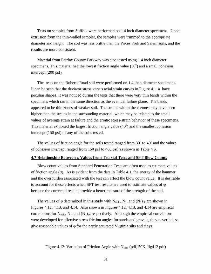
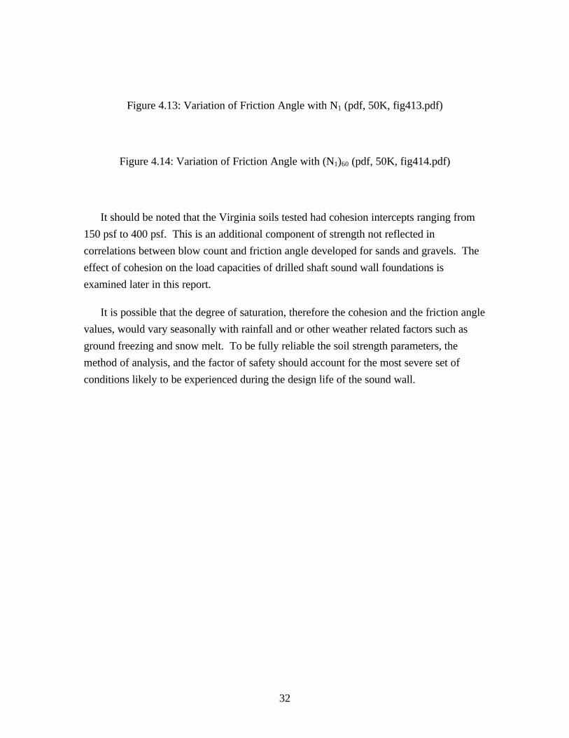
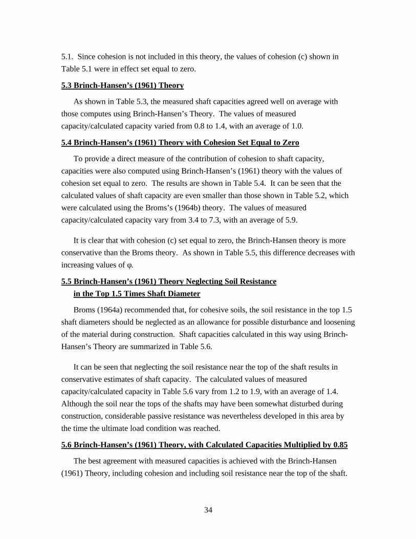
The values of φ determined in this study with Nfield, N1, and (N1)60 are shown in

Figures 4.12, 4.13, and 4.14. Also shown in Figures 4.12, 4.13, and 4.14 are empirical

correlations for Nfield, N1, and (N1)60 respectively. Although the empirical correlations

were developed for effective stress friction angles for sands and gravels, they nevertheless

give reasonable values of φ for the partly saturated Virginia silts and clays.

Figure 4.12: Variation of Friction Angle with Nfield (pdf, 50K, fig412.pdf)

32

Figure 4.13: Variation of Friction Angle with N1 (pdf, 50K, fig413.pdf)

Figure 4.14: Variation of Friction Angle with (N1)60 (pdf, 50K, fig414.pdf)

It should be noted that the Virginia soils tested had cohesion intercepts ranging from

150 psf to 400 psf. This is an additional component of strength not reflected in

correlations between blow count and friction angle developed for sands and gravels. The

effect of cohesion on the load capacities of drilled shaft sound wall foundations is

examined later in this report.

It is possible that the degree of saturation, therefore the cohesion and the friction angle

values, would vary seasonally with rainfall and or other weather related factors such as

ground freezing and snow melt. To be fully reliable the soil strength parameters, the

method of analysis, and the factor of safety should account for the most severe set of

conditions likely to be experienced during the design life of the sound wall.

33

CHAPTER 5 - COMPARISON OF MEASURED AND CALCULATED

ULTIMATE LATERAL LOAD CAPACITIES

5.1 Introduction

The field load tests described in Chapter 3, together with the triaxial compression tests

described in Chapter 4, provide a basis for evaluating the accuracy of Broms’s theory and

Brinch-Hansen’s theory for estimating the lateral load capacities of drilled shafts.

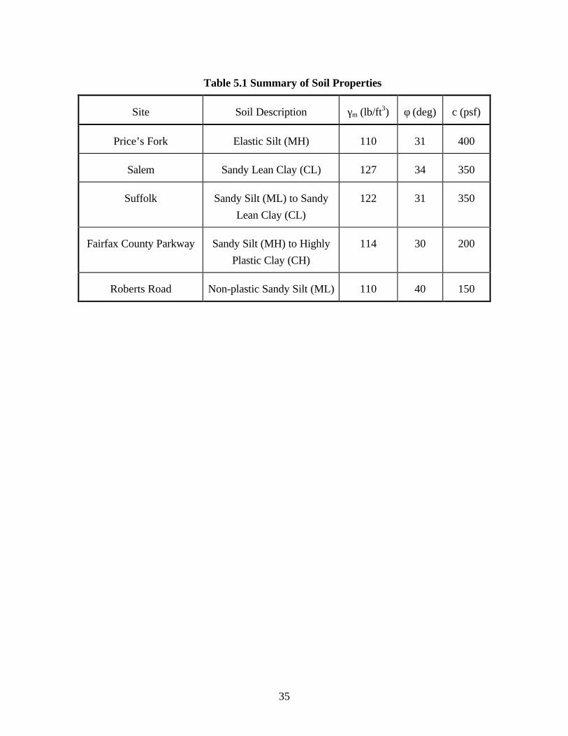
Drilled shaft capacities were calculated using the values of unit weight, cohesion

intercept, and angle of internal friction discussed in Chapter 4, which are summarized in

Table 5.1.

Capacities were calculated using five different methods:

1) Broms’s (1964b) theory for cohesionless soils, using the measured friction

angles and setting the cohesion values equal to zero.

2) Brinch-Hansen’s (1961) theory for soils with both cohesion and friction,

3) Brinch-Hansen’s (1961) theory with cohesion set equal to zero,

4) Brinch-Hansen’s (1961) theory neglecting soil resistance in the upper 1.5 times

shaft diameter, as recommended by Broms (1964a), and

5) Brinch-Hansen’s (1961) theory, multiplying calculated values of capacity by

0.85.

The capacities calculated using these methods are compared to the measured loads in

the following sections.

5.2 Broms’s (1964b) Theory

As shown in Table 5.2, the measured shaft capacities exceeded those calculated using

the Broms’s (1964b) theory by a considerable margin. The values of measured

capacity/calculated capacity varied from 3.1 to 4.4, with an average of 3.8.

These large differences between theory and measurement are due to the fact that the

Broms’s (1964b) theory is formulated for soils with no cohesion. The values of calculated

shaft capacity shown in Table 5.2 were computed using the values of φ shown in Table

34

5.1. Since cohesion is not included in this theory, the values of cohesion (c) shown in

Table 5.1 were in effect set equal to zero.

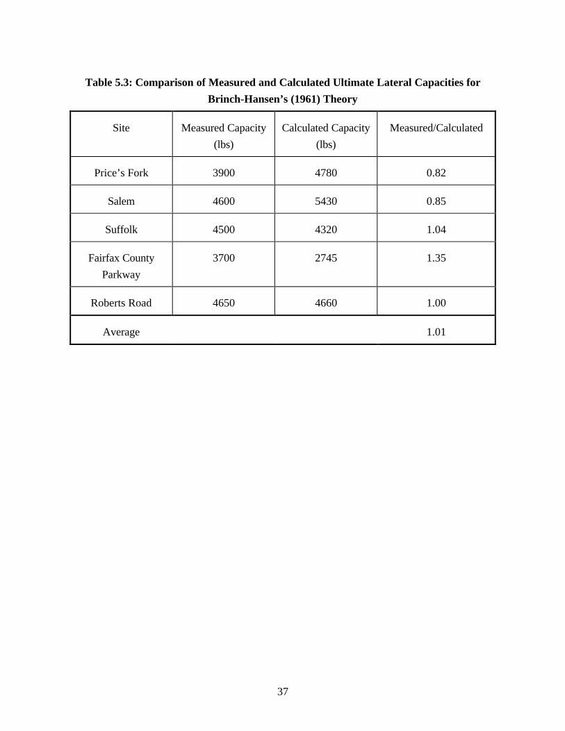
5.3 Brinch-Hansen’s (1961) Theory

As shown in Table 5.3, the measured shaft capacities agreed well on average with

those computes using Brinch-Hansen’s Theory. The values of measured

capacity/calculated capacity varied from 0.8 to 1.4, with an average of 1.0.

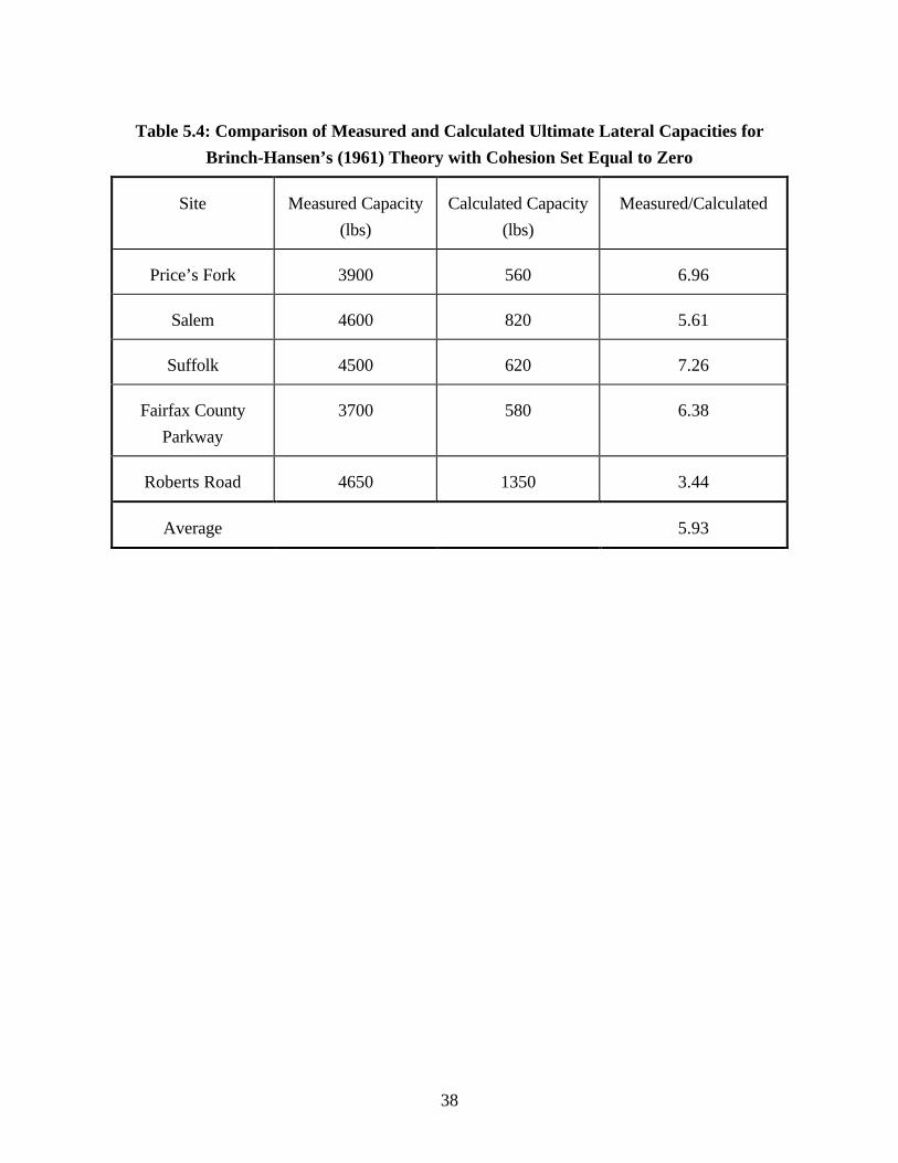
5.4 Brinch-Hansen’s (1961) Theory with Cohesion Set Equal to Zero

To provide a direct measure of the contribution of cohesion to shaft capacity,

capacities were also computed using Brinch-Hansen’s (1961) theory with the values of

cohesion set equal to zero. The results are shown in Table 5.4. It can be seen that the

calculated values of shaft capacity are even smaller than those shown in Table 5.2, which

were calculated using the Broms’s (1964b) theory. The values of measured

capacity/calculated capacity vary from 3.4 to 7.3, with an average of 5.9.

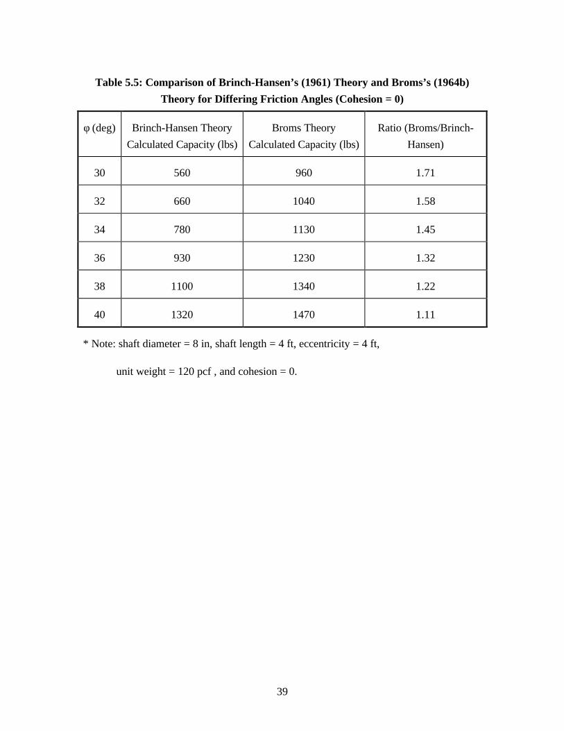
It is clear that with cohesion (c) set equal to zero, the Brinch-Hansen theory is more

conservative than the Broms theory. As shown in Table 5.5, this difference decreases with

increasing values of φ.

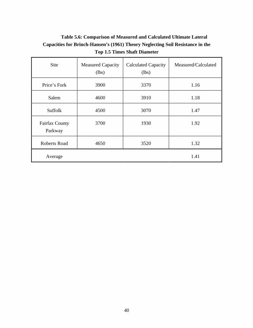
5.5 Brinch-Hansen’s (1961) Theory Neglecting Soil Resistance

in the Top 1.5 Times Shaft Diameter

Broms (1964a) recommended that, for cohesive soils, the soil resistance in the top 1.5

shaft diameters should be neglected as an allowance for possible disturbance and loosening

of the material during construction. Shaft capacities calculated in this way using Brinch-

Hansen’s Theory are summarized in Table 5.6.

It can be seen that neglecting the soil resistance near the top of the shaft results in

conservative estimates of shaft capacity. The calculated values of measured

capacity/calculated capacity in Table 5.6 vary from 1.2 to 1.9, with an average of 1.4.

Although the soil near the tops of the shafts may have been somewhat disturbed during

construction, considerable passive resistance was nevertheless developed in this area by

the time the ultimate load condition was reached.

5.6 Brinch-Hansen’s (1961) Theory, with Calculated Capacities Multiplied by 0.85

The best agreement with measured capacities is achieved with the Brinch-Hansen

(1961) Theory, including cohesion and including soil resistance near the top of the shaft.

35

Table 5.1 Summary of Soil Properties

Site Soil Description γm (lb/ft3) φ (deg) c (psf)

Price’s Fork Elastic Silt (MH) 110 31 400

Salem Sandy Lean Clay (CL) 127 34 350

Suffolk Sandy Silt (ML) to Sandy

Lean Clay (CL)

122 31 350

Fairfax County Parkway Sandy Silt (MH) to Highly

Plastic Clay (CH)

114 30 200

Roberts Road Non-plastic Sandy Silt (ML) 110 40 150

36

Table 5.2: Comparison of Measured and Calculated Ultimate Lateral Capacities for

Broms’s (1964b) Theory

Site Measured Capacity

(lbs)

Calculated Capacity

(lbs)

Measured/Calculated

Price’s Fork 3900 920 4.24

Salem 4600 1180 3.90

Suffolk 4500 1020 4.41

Fairfax County

Parkway

3700 1030 3.59

Roberts Road 4650 1520 3.06

Average 3.84

37

Table 5.3: Comparison of Measured and Calculated Ultimate Lateral Capacities for

Brinch-Hansen’s (1961) Theory

Site Measured Capacity

(lbs)

Calculated Capacity

(lbs)

Measured/Calculated

Price’s Fork 3900 4780 0.82

Salem 4600 5430 0.85

Suffolk 4500 4320 1.04

Fairfax County

Parkway

3700 2745 1.35

Roberts Road 4650 4660 1.00

Average 1.01

38

Table 5.4: Comparison of Measured and Calculated Ultimate Lateral Capacities for

Brinch-Hansen’s (1961) Theory with Cohesion Set Equal to Zero

Site Measured Capacity

(lbs)

Calculated Capacity

(lbs)

Measured/Calculated

Price’s Fork 3900 560 6.96

Salem 4600 820 5.61

Suffolk 4500 620 7.26

Fairfax County

Parkway

3700 580 6.38

Roberts Road 4650 1350 3.44

Average 5.93

39

Table 5.5: Comparison of Brinch-Hansen’s (1961) Theory and Broms’s (1964b)

Theory for Differing Friction Angles (Cohesion = 0)

φ (deg) Brinch-Hansen Theory

Calculated Capacity (lbs)

Broms Theory

Calculated Capacity (lbs)

Ratio (Broms/Brinch-

Hansen)

30 560 960 1.71

32 660 1040 1.58

34 780 1130 1.45

36 930 1230 1.32

38 1100 1340 1.22

40 1320 1470 1.11

* Note: shaft diameter = 8 in, shaft length = 4 ft, eccentricity = 4 ft,

unit weight = 120 pcf , and cohesion = 0.

40

Table 5.6: Comparison of Measured and Calculated Ultimate Lateral

Capacities for Brinch-Hansen’s (1961) Theory Neglecting Soil Resistance in the

Top 1.5 Times Shaft Diameter

Site Measured Capacity

(lbs)

Calculated Capacity

(lbs)

Measured/Calculated

Price’s Fork 3900 3370 1.16

Salem 4600 3910 1.18

Suffolk 4500 3070 1.47

Fairfax County

Parkway

3700 1930 1.92

Roberts Road 4650 3520 1.32

Average 1.41

41

As shown in Table 5.3, the average value of measured capacity/calculated capacity for this

case is 1.0.

Although capacities calculated using the Brinch-Hansen (1961) theory are close to the

measured values on average, the measured values were smaller than the calculated values

for Prices’ Fork and Salem. As shown in Table 5.7, the reliability of Brinch-Hansen’s

(1961) theory can be improved if the theoretical values are reduced by 15% (multiplied by

0.85). When this is done, the values of measured capacity/calculated capacity vary from

1.0 to 1.6, with an average of 1.2.

5.7 Summary

Based on these comparisons between measured and calculated capacities, the

following conclusions appear to be justified:

1. Broms’s (1964b) theory, which is formulated for cohesionless soils,

underestimates the capacities measured at all five sites where tests were

performed.

2. The contribution of cohesion to the capacities of the test shafts is quite large.

Note however, that the percentage contribution of cohesion to shaft capacity

decreases as shaft size increases, as discussed in Chapter 6.

3. Brinch-Hansen’s (1961) theory, which includes both cohesion and friction

angle, provides an accurate measure of estimating shaft capacities, on average.

The theory slightly overestimates shaft capacities for the Price’s Fork and

Salem sites.

4. The reliability of Brinch-Hansen’s (1961) theory can be improved if the

theoretical capacities are reduced by 15% (i.e. if the theoretical capacities are

multiplied by 0.85).

On the basis of these comparisons, it is recommended that reliable and reasonably

accurate estimates of shaft capacity can be made by:

• Using Brinch-Hansen’s (1961) theory.

• Including cohesion as well as friction.

• Including soil resistance near the top of the shaft.

42

• Reducing the calculated values by 15% to improve reliability.

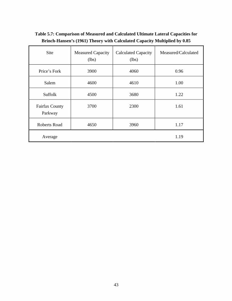
43

Table 5.7: Comparison of Measured and Calculated Ultimate Lateral Capacities for

Brinch-Hansen’s (1961) Theory with Calculated Capacity Multiplied by 0.85

Site Measured Capacity

(lbs)

Calculated Capacity

(lbs)

Measured/Calculated

Price’s Fork 3900 4060 0.96

Salem 4600 4610 1.00

Suffolk 4500 3680 1.22

Fairfax County

Parkway

3700 2300 1.61

Roberts Road 4650 3960 1.17

Average 1.19

44

CHAPTER 6 - EFFECTS OF ANALYSIS PROCEDURES

AND PARAMETER VALUES

6.1 Introduction

A parametric study was performed to assess the effect of various factors on the

required shaft length. The study was performed using the program LCAP, described in

Appendix C. Wall heights of 15 feet and 30 feet were used in the study, together with a

wind speed of 80 mph, and exposure category D. Shown in Table 6.1 are the specific

values used in the study. The effects of the analysis procedures and parameter values are

summarized in the following paragraphs.

6.2 Effect of Theory Used in the Analysis

Analyses performed using Brinch-Hansen's (1961) theory for c = 0 usually result in

shaft lengths that are longer than those found using Broms's (1964b) theory. The

difference is greatest for larger shaft diameters, and may be as much as 50%.

6.3 Effect of Cohesion

When cohesion is included in Brinch-Hansen's (1961) theory, the resulting shaft

lengths may be longer or shorter than those found using Broms's (1964b) theory with c =

0. Shaft lengths calculated using Brinch-Hansen's (1961) theory with c = 150 psf range

from 20% shorter to 20% longer than those calculated using Broms's (1964b) theory with

c = 0. Shaft lengths calculated using c = 400 psf in Brinch-Hansen's (1961) theory are

shorter than those calculated using Broms's (1964b) theory with c = 0. The difference is

as much 40%, and the difference tends to be greater for small shaft diameters.

6.4 Effect of Sloping Ground

Method 1 for including the effect of ground slope in analyses (the method cited in the

AASHTO Guide Specifications for the Structural Design of Sound Barriers, 1992, and

discussed in Appendix C) is based on fundamental soil mechanics principles. Method 2

(suggested by Boghrat, 1990 and discussed in Appendix C) results in shaft lengths which

are as much as 20% longer than those found using Method 1. Method 2 thus appears to

be excessively conservative.

For 2:1 ground slope, shaft lengths calculated using Broms's (1964b) theory are 50%

longer than those found for level ground conditions. For Brinch-Hansen's (1961) theory,

shaft lengths for 2:1 ground slope are about 30% longer than for level ground conditions.

(These effects were evaluated using Method 1.)

45

6.5 Effect of Ignoring Soil Resistance at the Top of the Shaft

For cohesionless soils, neglecting the soil resistance in the top 2 feet results in shaft

lengths that are 2% to 8% longer than those found when this resistance is included. The

effect is greatest for large diameter shafts.

The effect of ignoring soil resistance at the top of the shaft is greater for soils that have

cohesion. For c = 400 psf, ignoring soil resistance in the upper 2 feet results in 15% to

20% longer shafts.

6.6 Effect of Soil Friction Angle, φφ

Reducing φ by 2 degrees results in shaft lengths that are 3% to 4% longer as computed

by Broms's (1964b) theory, and 6% to 7% longer as computed by Brinch-Hansen's (1961)

theory.

6.7 Effect of Changing the Factor of Safety

The factor of safety is applied by multiplying the total horizontal load and the total

moment by the factor of safety before the required shaft length is calculated. Increasing

the factor of safety from 1.88 to 2.50 results in a 10% to 15% increase in the required

shaft length.

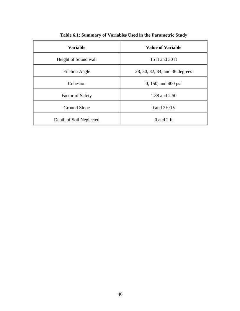
46

Table 6.1: Summary of Variables Used in the Parametric Study

Variable Value of Variable

Height of Sound wall 15 ft and 30 ft

Friction Angle 28, 30, 32, 34, and 36 degrees

Cohesion 0, 150, and 400 psf

Factor of Safety 1.88 and 2.50

Ground Slope 0 and 2H:1V

Depth of Soil Neglected 0 and 2 ft

47

CHAPTER 7 - CONCLUSION

The study described in the previous chapters was performed to investigate the factors

that affect the accuracy of the procedures being used by VDOT and its contractors for

design of drilled shaft sound wall foundations in Virginia. The following conclusions can

be drawn from the study:

1. Published correlations between SPT blow counts and friction angles, shown in Figure

4.12, 4.13, and 4.14, appear to be reasonable for estimating friction angles for the silty

and clayey soils found in many locations in Virginia. The accuracy of the correlations

appears to be best if the blow counts are corrected for overburden pressure and

hammer energy, that is, if φ is estimated using (N1)60 values.

2. The undrained strengths of the partly saturated silts and clays from five test sites in

Virginia are characterized by cohesion values varying from 150 psf to 400 psf, and

friction angles varying from 30 degrees to 40 degrees. Both cohesion and friction can

be included in ultimate load analyses if Brinch-Hansen’s (1961) theory is used.

Although this theory is too cumbersome for easy use by hand, it can be applied readily

through the EXCEL spreadsheet LCAP, which was developed during the study.

Although the contribution of cohesion was found to be a significant factor in the

failure loads measured in 20 load tests performed on eight inch diameter and nine inch

diameter drilled shafts, calculations using Brinch-Hansen’s (1961) theory show that

the contribution of cohesion to the ultimate load capacity would be less important for

shafts of larger diameter.

The two most logical alternatives for design of drilled shaft sound wall foundations in

Virginia appear to be (a) Using Brinch-Hansen’s (1961) theory and including the

cohesive component of strength as well as friction, or (b) Using Broms’s (1964b)

theory and ignoring cohesion (setting c = 0). Both of these theories are included in the

spreadsheet LCAP.

Using Brinch-Hansen’s (1961) theory requires that the value of c as well as φ be

measured or estimated. Measuring c would involve performing triaxial tests on the

foundation soil, which would add to the time and cost required for drilled shaft

foundation design. Estimating values of c would require a more extensive database for

strengths of Virginia soils than is currently available.

48

Parametric studies show that if c = 150 psf, the required shaft lengths calculated using

Broms’s (1964b) theory without c are 20% longer to 20% shorter than those found

using Brinch-Hansen’s (1961) theory with c. If c = 400 psf the required shaft lengths

calculated using Broms’s (1964b) theory without c are as much as 40% greater than

those found using Brinch-Hansen’s (1961) theory with c.

3. Using Broms’s (1964b) theory, in combination with factors of safety of 1.88 and 2.50,

results in safe designs of drilled shaft sound wall foundations in Virginia soils,

provided the value of φ used in the calculations is representative of the foundation soil.

It seems logical to use F = 1.88 when the characteristics of the foundation soil are

reliably known, and to use F = 2.50 when there is greater uncertainty about the

foundation soil conditions.

4. The spreadsheet program LCAP, described in Appendix C, provides an effective

computational tool for the design of drilled shaft sound wall foundations. It calculates

loads on sound wall foundations from input wind speeds, exposure categories, and

sound wall dimensions; performs analyses using both Broms’s (1964b) theory and

Brinch-Hansen’s (1961) theory; and includes calculations for sloping and level ground

conditions. It provides shaft lengths, concrete volumes, and bending moments for

shaft diameters ranging from 18 inches to 54 inches.

LCAP provides an engineer designing drilled shaft sound wall foundations , or

checking designs, an effective tool for performing computations efficiently, for rapidly

assessing the effects of possible changes in conditions, and, through these processes,

for applying engineering judgment effectively.

5. The principal shortcomings of the field load test program performed during this study

relate to the small size of the drilled shafts that were tested, and the fact that only a

few cyclic load tests were performed. It would be desirable to extend this study by

testing larger-size drilled shafts, and by subjecting them to extensive cyclic loading.

Such studies would further reduce uncertainties in design of drilled shaft sound wall

foundations in Virginia.

49

REFERENCES

“1992 Revisions to Guide Specifications for Structural Design of Sound Barriers,” (1992),

AASHTO, Washington D.C., 38 p.

“Guide Specifications for Structural Design of Sound Barriers,” (1989), AASHTO,

Washington D.C., 38 p.

Bierschwale, M.W., Cole, H.M., and Bartoskewitz, R.E. (1981), "Lateral Load Tests on

Drilled Shafts," Drilled Piers and Caissons, Ed. M.W. O'Neill, ASCE New York,

pp. 98-113.

Boghrat, A. (1990), “Sound Barrier Wall Foundations in Granular Material,”

Transportation Research Record 1288, pp. 158-167.

Brinch-Hansen, J., (1961), “The Ultimate Resistance of Rigid Piles Against Transversal

Forces,” Bulletin No. 12, Geoteknisk Institut (The Danish Geotechnical Institute),

Copenhagen, pp. 5-9.

Broms, B.B. (1964a), “Lateral Resistance of Piles in Cohesive Soils,” Journal of the Soil

Mechanics and Foundations Division , ASCE, Vol. 90 SM2, pp. 27-63.

Broms, B.B. (1964b), “Lateral Resistance of Piles in Cohesionless Soils,” Journal of the

Soil Mechanics and Foundations Division, ASCE, Vol. 90 SM3, pp. 123-156.

Duncan, J.M., Horz, R.C., and Yang, T.L. (1989), Shear Strength Correlations for

Geotechnical Engineering, Virginia Polytechnic Institute and State University,

Blacksburg, 100p.

Evans, L.T., and Duncan, J.M. (1982), “Simplified Analysis of Laterally Loaded Piles,”

Report No. UCB/GT/82-04, Department of Civil Engineering University of

California at Berkeley, 224 p.

50

Fang, Y.S., Chen, J.M., and Chen, C.Y. (1997) “Earth Pressures with Sloping Backfill,”

Journal of Geotechnical and Geoenvironmental Engineering, ASCE, Vol. 123 No.

3, pp. 250-259.

Kovacs, William D. (1994), "Effects of SPT Equipment and Procedures on the Design of

Shallow Foundations on Sand," Proceedings of Settlement 1994: Vertical and

Horizontal Deformations of Foundations and Embankments, ASCE, Volume 1,

pp. 121-131.

Lambe, T.W., and Whitman, R.V. (1969), Soil Mechanics, John Wiley and Sons, New

York, 553 p.

Lawler, A. (June 3, 1997) Personal Correspondence.

Mayne, P.W., Kulhawy, F.H., and Trautmann, C.H. (1992), "Experimental Study of

Undrained Lateral and Moment Behavior of Drilled Shafts During Static and

Cyclic Loading," Report TR-100221, Electric Power Research Institute, Palo Alto,

284 p.

Meyerhof, G.G. (1956), “Penetration Tests and Bearing Capacity of Cohesionless Soils,”

Journal of the Soil Mechanics and Foundations Division, ASCE, Vol. 82, No.

SM1, paper 866.

Peck, R.B., Hansen, W.E., and Thornburn, T.H. (1974), Foundation Engineering, 2nd Ed.,

John Wiley and Sons, Inc., New York, 514 p.

Poulos, H.G. and Davis, E.H., (1980), Pile Foundation Analysis and Design, John Wiley

and Sons, New York, 397 p.

Reese, L.C. and Wang, S.T. (1989), LPILE1, Microcomputer Program, Ensoft, Inc.,

Austin, Texas.

51

Sastry, V.V.R.N., and Meyerhof, G.G. (1986), “Lateral Soil Pressures and Displacements

of Rigid Piles in Homogeneous Soils Under Eccentric and Inclines Loads,”

Canadian Geotechnical Journal, No. 23, pp. 281-286.

Skempton, A.W. (1986), "Standard penetration test procedures and the effects in sands of

overburden pressure, relative density, particle size, ageing and overconsolidation,"

Geotechnique, 36, No. 3, pp. 425-447.

Terzaghi, K., and Peck, R. (1967), Soil Mechanics in Engineering Practice, 2nd Edition,

John Wiley and Sons, New York, 729 p.

Terzaghi, K., Peck, R.B., and Mesri, G. (1996), Soil Mechanics in Engineering Practice,

3rd Ed., John Wiley and Sons, Inc., New York, 549p.

52

APPENDIX A - EQUATIONS FOR Kq AND Kc FACTORS FOR

THE BRINCH-HANSEN’S (1961) THEORY

A.1 Introduction

Included in this Appendix are the equations used to calculate the earth pressure

coefficients for Brinch-Hansen’s (1961) theory. The assumptions involved with these

factors are discussed in Chapter 2.

A.2 Equations for Kq and Kc

KK + K

z

D

1+z

D

q

qo

q q

q

=

∞α

α(A.1)

where:

Kq = passive earth pressure coefficient due to weight of soil at intermediate depth,

K = passive earth pressure coefficient due to weight of soil at ground surface,qo

K = (e cos tan(45 +1

2))

e ))

qo (

1

2+ )tan o

-(1

2- )tan o

π φ φ

π φ φ

φ φ

φ φ

−

−( cos tan(451

2

K = passive earth pressure coefficient due to weight of soil at great depth,q∞

K N d Kq c c o∞ ∞= tanφ ,

αφ

φq

qo

o

q qo o

=K K sin

(K - K )sin(45 +1

2)∞

z = depth below ground (units of length),

D = shaft diameter (units of length),

Ko = at-rest earth pressure,

Ko = 1 - sinφ, and

φ = friction angle of foundation soil.

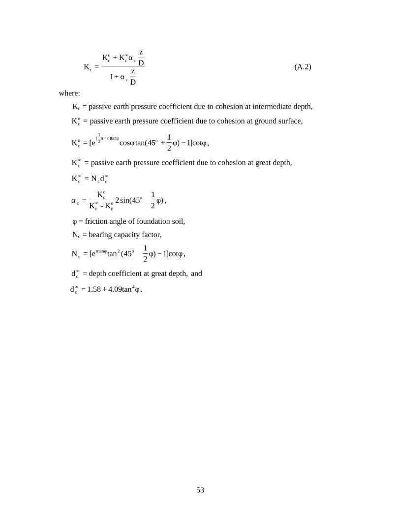
53

KK + K

z

D

1+z

D

c

co

c c

c

=

∞α

α(A.2)

where:

Kc = passive earth pressure coefficient due to cohesion at intermediate depth,

K = passive earth pressure coefficient due to cohesion at ground surface,co

K = [e cos +1

cotco (

1

2+ )tan oπ φ φ

φ φ φtan( ) ]452

1− ,

K = passive earth pressure coefficient due to cohesion at great depth,c∞

K N dc c c∞ ∞=

α φcco

c co

oK

K - K)= +∞ 2 45

1

2sin( ,

φ = friction angle of foundation soil,

Nc = bearing capacity factor,

N [e tan cotctan 2 o= + −π φ φ φ( ) ]45

1

21 ,

d = depth coefficient at great depth, andc∞

d = 1.58 + 4.09tanc4∞ φ .

54

APPENDIX B - WIND PRESSURES AND WIND LOADS

FOR DESIGN OF SOUND BARRIERS

B.1 Introduction

Wind load conditions are of critical importance in the design of sound walls. This

appendix describes the procedure used in calculating wind pressures and wind loads in

LCAP. These procedure are based on the “Guide Specifications for Structural Design of

Sound Barriers,” 1989 and 1992 Revisions.

B.2 Wind Pressures

Sound walls are designed for wind pressures resulting from 50-year recurrence interval

wind speeds. These vary from 70 mph in the southwest corner of Virginia to 95 mph in

the southeast corner. The wind pressure is calculated using the expression:

P = 0.00256(1.3V) C C2d c (B.1)

where:

P = wind pressure (psf),

V = wind speed (mph) based on a 50 year mean recurrence interval,

(1.3V) = 30% gust speed,

Cd = drag coefficient (1.2 for sound barriers), and

Cc = combined height, exposure, and location coefficient.

The exposure categories are:

Exposure B1 - urban and suburban areas with numerous closely spaced

obstructions, having the size of single-family dwellings or larger, that prevail in the

upwind direction from the sound barrier for distance of at least 1500 feet.

Exposure B2- Urban and suburban areas with more open terrain not meeting the

requirements of Exposure B1.

Exposure C - Open terrain with scattered obstructions. This category includes flat,

open country and grasslands. This exposure is used for sound barriers located on

bridge structures, retaining walls, or traffic barriers.

55

Exposure D - Flat unobstructed coastal areas directly exposed to wind flowing

over large bodies of water, extending inland from the shoreline a distance of one

half mile.

Table B.1 gives values of Cc for four different exposure categories and for differing

wall heights.

B.3 Wind Loads

The loads on sound barrier walls are calculated by multiplying the wind pressure by the

tributary area:

Wt = P1A1 + P2A2 + P3A3 (B.2)

where:

Wt = total wind load (lbs),

P1, P2, P3 = wind pressures for height zone 1, 2, and 3, and

A1, A2, A3 = areas for height zones 1, 2, and 3.

The area for each height zone is calculated by multiplying the vertical distance from

the bottom of the height zone to the top of the height zone by the distance between drilled

shafts:

A = ∆Y•L (B.3)

where:

∆Y = vertical distance from bottom to top of height zone as shown in Figure B.1 (ft), and

L = horizontal distance (spacing) between foundations (ft). If the spacing varies, the valueof L for a particular shaft is the average of the values for adjacent shafts.

Figure B.1 shows the distribution of pressure on a sound barrier, and the procedure

used to convert the pressure to a total horizontal load and total moment on the drilled

shaft.

Figure B.2 shows an example calculation for wind loads on a sound barrier.

Figure B.1: Moments and Loads on Sound Wall Foundations due to Wind (pdf, 100K,

figb1.pdf)

56

Figure B.2: Example Calculation of Wind Load (pdf, 50K, figb2.pdf)

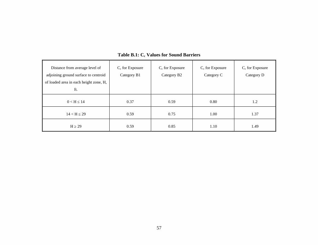
57

Table B.1: Cc Values for Sound Barriers

Distance from average level of

adjoining ground surface to centroid

of loaded area in each height zone, H,

ft.

Cc for Exposure

Category B1

Cc for Exposure

Category B2

Cc for Exposure

Category C

Cc for Exposure

Category D

0 < H ≤ 14 0.37 0.59 0.80 1.2

14 < H ≤ 29 0.59 0.75 1.00 1.37

H ≥ 29 0.59 0.85 1.10 1.49

58

APPENDIX C - DESIGN OF DRILLED SHAFT SOUND WALL FOUNDATIONS

USING THE SPREADSHEET LCAP

C.1 Introduction

A spreadsheet named LCAP was developed for use in the design of drilled shaft sound wall

foundations. LCAP was programmed in Microsoft Excel to perform analyses using both the

Broms (1964b) theory and the Brinch-Hansen (1961) theory. A reduction factor of 15% is

applied to values of Pult for the Brinch-Hansen (1961) theory, based on field load tests on

eccentrically loaded drilled shafts performed in this study.

C.2 Input for LCAP

Copies of printed input and output from LCAP are shown in Figures C.1 and C.2. This

information appears on screen as the spreadsheet is being used, and can be printed by pressing

control-s (s for sloping ground) for the section of the spreadsheet shown in Figure C.1 or control-

l (l for level ground) for the section of the spreadsheet shown in Figure C.2.

The input values that define the problem are typed in the tables shown in the upper left areas

of Figures C.1 and C.2. All of the other cells in the spreadsheet, except the user’s name and the

project name, are locked, and cannot be altered except by changing the input data values.

As shown in the upper left area in of Figure C.1, the values input to define sloping ground

conditions for analysis are:

• wind speed (mph),

• drag coefficient (dimensionless) = 1.2 for sound walls, (Appendix B),

• exposure category, (Appendix B),

• wall height (ft),

• shaft spacing (ft),

• additional horizontal load (lbs),

• eccentricity of additional load (ft),

• cohesion of foundation soil (psf),

• friction angle of foundation soil (degrees),

59

• unit weight of foundation soil (pcf),

• slope of ground surface on downhill side of the sound wall (degrees),

• factor of safety, and

• depth over which soil resistance at top of shaft is neglected (ft).

For level ground conditions, the ground slope can be set equal to zero, or the level ground

section of the sheet, shown in Figure C.2, can be used. Using the level ground section of the

sheet for zero ground slope conditions has the advantage that the results section of this part of the

sheet are more compact, being tailored for the level ground condition. The same results are

calculated, whichever procedure is followed.

Using the input variables listed above, values of design load, moment, and eccentricity are

computed as displayed in the upper right portion of Figures C.1 and C.2

C.3 Components of LCAP

The spreadsheet LCAP consists of a series of worksheets which perform specific operations.

The specific function of each worksheet is given below:

• Main Module - consists of tables for input of design variables for display of computed

results.

• BrinchHansen1 - performs calculations for shaft diameters of 18 inches and 24 inches

for Brinch-Hansen’s (1961) theory using Method 1 to account for sloping ground

effects.

• BrinchHansen2 - performs calculations for shaft diameters of 30 inches and 36 inches

for Brinch-Hansen’s (1961) theory using Method 1 to account for sloping ground

effects.

• BrinchHansen3 - performs calculations for shaft diameters of 42 inches and 48 inches

for Brinch-Hansen’s (1961) theory using Method 1 to account for sloping ground

effects.

• BrinchHansen4 - performs calculations for a shaft diameter of 54 inches for Brinch-

Hansen’s (1961) theory using Method 1 to account for sloping ground effects.

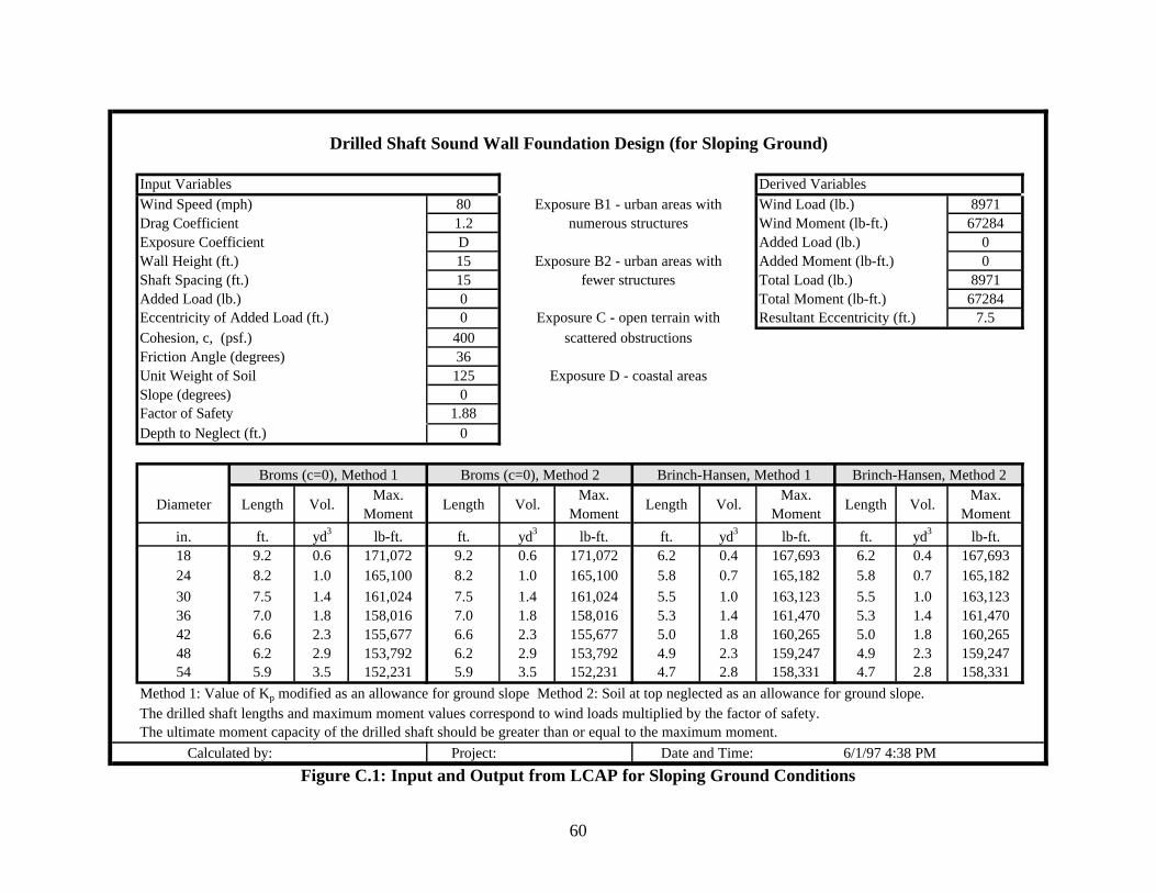
60

Drilled Shaft Sound Wall Foundation Design (for Sloping Ground)

Input Variables Derived VariablesWind Speed (mph) 80 Exposure B1 - urban areas with Wind Load (lb.) 8971Drag Coefficient 1.2 numerous structures Wind Moment (lb-ft.) 67284Exposure Coefficient D Added Load (lb.) 0Wall Height (ft.) 15 Exposure B2 - urban areas with Added Moment (lb-ft.) 0Shaft Spacing (ft.) 15 fewer structures Total Load (lb.) 8971Added Load (lb.) 0 Total Moment (lb-ft.) 67284Eccentricity of Added Load (ft.) 0 Exposure C - open terrain with Resultant Eccentricity (ft.) 7.5Cohesion, c, (psf.) 400 scattered obstructionsFriction Angle (degrees) 36Unit Weight of Soil 125 Exposure D - coastal areasSlope (degrees) 0Factor of Safety 1.88Depth to Neglect (ft.) 0

Broms (c=0), Method 1 Broms (c=0), Method 2 Brinch-Hansen, Method 1 Brinch-Hansen, Method 2

Diameter Length Vol.Max.

MomentLength Vol.

Max. Moment

Length Vol.Max.

MomentLength Vol.

Max. Moment

in. ft. yd3 lb-ft. ft. yd3 lb-ft. ft. yd3 lb-ft. ft. yd3 lb-ft.18 9.2 0.6 171,072 9.2 0.6 171,072 6.2 0.4 167,693 6.2 0.4 167,69324 8.2 1.0 165,100 8.2 1.0 165,100 5.8 0.7 165,182 5.8 0.7 165,182

30 7.5 1.4 161,024 7.5 1.4 161,024 5.5 1.0 163,123 5.5 1.0 163,12336 7.0 1.8 158,016 7.0 1.8 158,016 5.3 1.4 161,470 5.3 1.4 161,47042 6.6 2.3 155,677 6.6 2.3 155,677 5.0 1.8 160,265 5.0 1.8 160,26548 6.2 2.9 153,792 6.2 2.9 153,792 4.9 2.3 159,247 4.9 2.3 159,24754 5.9 3.5 152,231 5.9 3.5 152,231 4.7 2.8 158,331 4.7 2.8 158,331

Method 1: Value of Kp modified as an allowance for ground slope Method 2: Soil at top neglected as an allowance for ground slope.The drilled shaft lengths and maximum moment values correspond to wind loads multiplied by the factor of safety.The ultimate moment capacity of the drilled shaft should be greater than or equal to the maximum moment.

Calculated by: Project: Date and Time: 6/1/97 4:38 PM

Figure C.1: Input and Output from LCAP for Sloping Ground Conditions

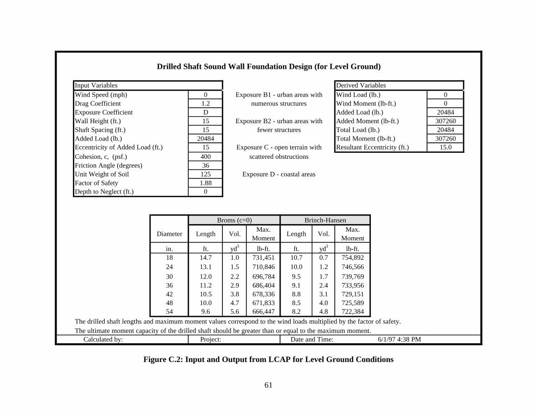
61

Drilled Shaft Sound Wall Foundation Design (for Level Ground)

Input Variables Derived VariablesWind Speed (mph) 0 Exposure B1 - urban areas with Wind Load (lb.) 0Drag Coefficient 1.2 numerous structures Wind Moment (lb-ft.) 0Exposure Coefficient D Added Load (lb.) 20484Wall Height (ft.) 15 Exposure B2 - urban areas with Added Moment (lb-ft.) 307260Shaft Spacing (ft.) 15 fewer structures Total Load (lb.) 20484Added Load (lb.) 20484 Total Moment (lb-ft.) 307260Eccentricity of Added Load (ft.) 15 Exposure C - open terrain with Resultant Eccentricity (ft.) 15.0Cohesion, c, (psf.) 400 scattered obstructionsFriction Angle (degrees) 36Unit Weight of Soil 125 Exposure D - coastal areasFactor of Safety 1.88Depth to Neglect (ft.) 0

Broms (c=0) Brinch-Hansen

Diameter Length Vol.Max.

MomentLength Vol.

Max. Moment

in. ft. yd3 lb-ft. ft. yd3 lb-ft.18 14.7 1.0 731,451 10.7 0.7 754,89224 13.1 1.5 710,846 10.0 1.2 746,566

30 12.0 2.2 696,784 9.5 1.7 739,76936 11.2 2.9 686,404 9.1 2.4 733,95642 10.5 3.8 678,336 8.8 3.1 729,15148 10.0 4.7 671,833 8.5 4.0 725,58954 9.6 5.6 666,447 8.2 4.8 722,384

The drilled shaft lengths and maximum moment values correspond to the wind loads multiplied by the factor of safety.The ultimate moment capacity of the drilled shaft should be greater than or equal to the maximum moment.

Calculated by: Project: Date and Time: 6/1/97 4:38 PM

Figure C.2: Input and Output from LCAP for Level Ground Conditions

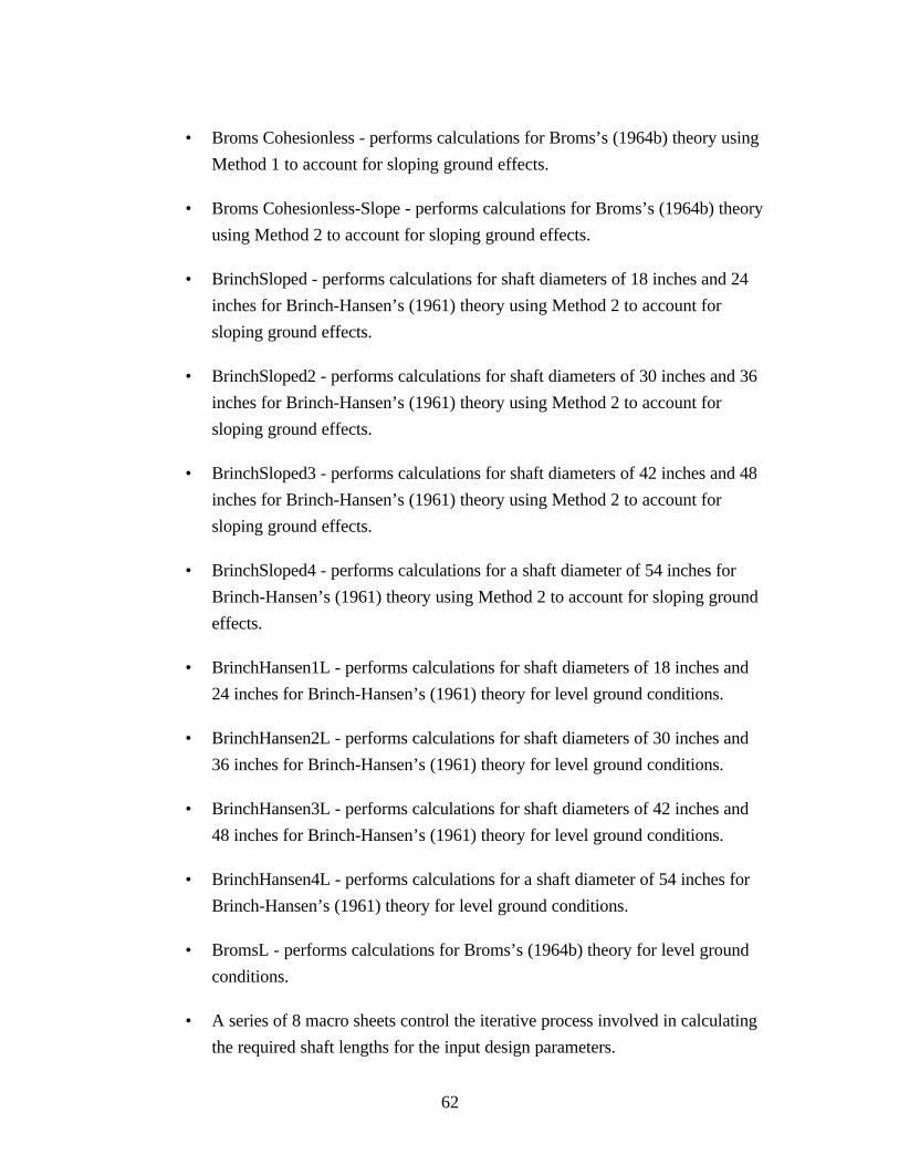
62

• Broms Cohesionless - performs calculations for Broms’s (1964b) theory using

Method 1 to account for sloping ground effects.

• Broms Cohesionless-Slope - performs calculations for Broms’s (1964b) theory

using Method 2 to account for sloping ground effects.

• BrinchSloped - performs calculations for shaft diameters of 18 inches and 24

inches for Brinch-Hansen’s (1961) theory using Method 2 to account for

sloping ground effects.

• BrinchSloped2 - performs calculations for shaft diameters of 30 inches and 36

inches for Brinch-Hansen’s (1961) theory using Method 2 to account for

sloping ground effects.

• BrinchSloped3 - performs calculations for shaft diameters of 42 inches and 48

inches for Brinch-Hansen’s (1961) theory using Method 2 to account for

sloping ground effects.

• BrinchSloped4 - performs calculations for a shaft diameter of 54 inches for

Brinch-Hansen’s (1961) theory using Method 2 to account for sloping ground

effects.

• BrinchHansen1L - performs calculations for shaft diameters of 18 inches and

24 inches for Brinch-Hansen’s (1961) theory for level ground conditions.

• BrinchHansen2L - performs calculations for shaft diameters of 30 inches and

36 inches for Brinch-Hansen’s (1961) theory for level ground conditions.

• BrinchHansen3L - performs calculations for shaft diameters of 42 inches and

48 inches for Brinch-Hansen’s (1961) theory for level ground conditions.

• BrinchHansen4L - performs calculations for a shaft diameter of 54 inches for

Brinch-Hansen’s (1961) theory for level ground conditions.

• BromsL - performs calculations for Broms’s (1964b) theory for level ground

conditions.

• A series of 8 macro sheets control the iterative process involved in calculating

the required shaft lengths for the input design parameters.

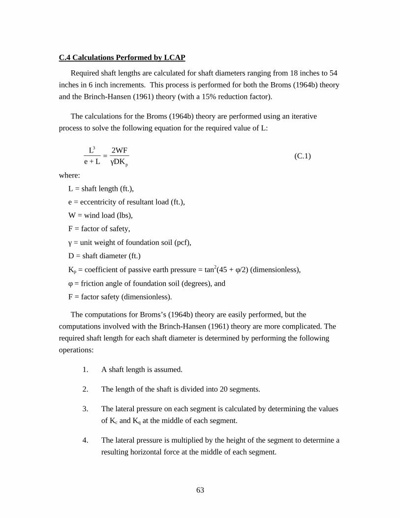
63

C.4 Calculations Performed by LCAP

Required shaft lengths are calculated for shaft diameters ranging from 18 inches to 54

inches in 6 inch increments. This process is performed for both the Broms (1964b) theory

and the Brinch-Hansen (1961) theory (with a 15% reduction factor).

The calculations for the Broms (1964b) theory are performed using an iterative

process to solve the following equation for the required value of L:

L

e + L

2WF

DK

3

p

=γ

(C.1)

where:

L = shaft length (ft.),

e = eccentricity of resultant load (ft.),

W = wind load (lbs),

F = factor of safety,

γ = unit weight of foundation soil (pcf),

D = shaft diameter (ft.)

Kp = coefficient of passive earth pressure = tan2(45 + φ/2) (dimensionless),

φ = friction angle of foundation soil (degrees), and

F = factor safety (dimensionless).

The computations for Broms’s (1964b) theory are easily performed, but the

computations involved with the Brinch-Hansen (1961) theory are more complicated. The

required shaft length for each shaft diameter is determined by performing the following

operations:

1. A shaft length is assumed.

2. The length of the shaft is divided into 20 segments.

3. The lateral pressure on each segment is calculated by determining the values

of Kc and Kq at the middle of each segment.

4. The lateral pressure is multiplied by the height of the segment to determine a

resulting horizontal force at the middle of each segment.

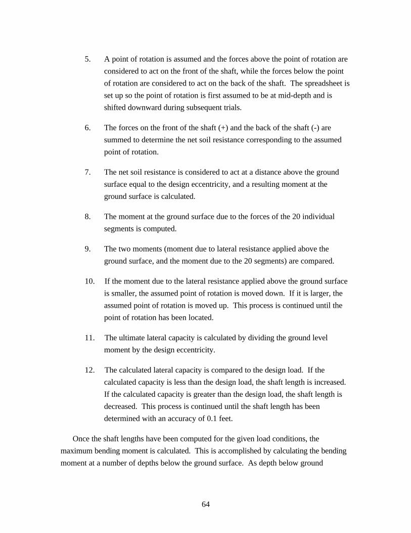
64

5. A point of rotation is assumed and the forces above the point of rotation are

considered to act on the front of the shaft, while the forces below the point

of rotation are considered to act on the back of the shaft. The spreadsheet is

set up so the point of rotation is first assumed to be at mid-depth and is

shifted downward during subsequent trials.

6. The forces on the front of the shaft (+) and the back of the shaft (-) are

summed to determine the net soil resistance corresponding to the assumed

point of rotation.

7. The net soil resistance is considered to act at a distance above the ground

surface equal to the design eccentricity, and a resulting moment at the

ground surface is calculated.

8. The moment at the ground surface due to the forces of the 20 individual

segments is computed.

9. The two moments (moment due to lateral resistance applied above the

ground surface, and the moment due to the 20 segments) are compared.

10. If the moment due to the lateral resistance applied above the ground surface

is smaller, the assumed point of rotation is moved down. If it is larger, the

assumed point of rotation is moved up. This process is continued until the

point of rotation has been located.

11. The ultimate lateral capacity is calculated by dividing the ground level

moment by the design eccentricity.

12. The calculated lateral capacity is compared to the design load. If the

calculated capacity is less than the design load, the shaft length is increased.

If the calculated capacity is greater than the design load, the shaft length is

decreased. This process is continued until the shaft length has been

determined with an accuracy of 0.1 feet.

Once the shaft lengths have been computed for the given load conditions, the

maximum bending moment is calculated. This is accomplished by calculating the bending

moment at a number of depths below the ground surface. As depth below ground

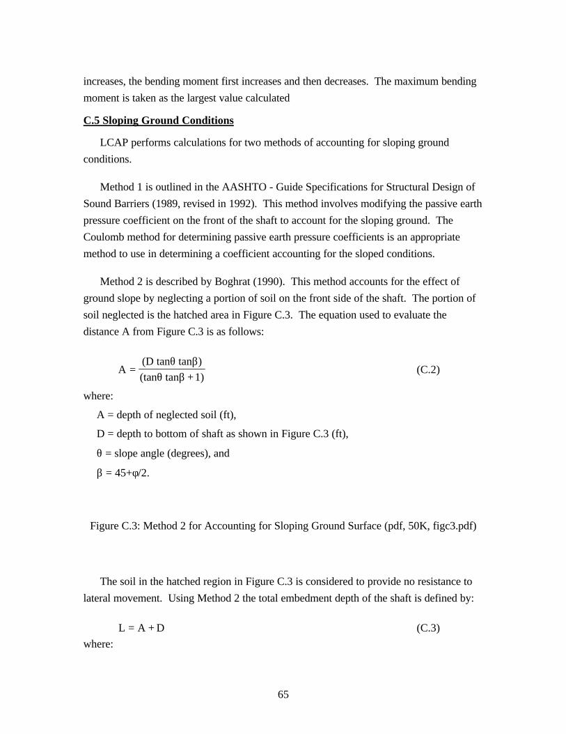
65

increases, the bending moment first increases and then decreases. The maximum bending

moment is taken as the largest value calculated

C.5 Sloping Ground Conditions

LCAP performs calculations for two methods of accounting for sloping ground

conditions.

Method 1 is outlined in the AASHTO - Guide Specifications for Structural Design of

Sound Barriers (1989, revised in 1992). This method involves modifying the passive earth

pressure coefficient on the front of the shaft to account for the sloping ground. The

Coulomb method for determining passive earth pressure coefficients is an appropriate

method to use in determining a coefficient accounting for the sloped conditions.

Method 2 is described by Boghrat (1990). This method accounts for the effect of

ground slope by neglecting a portion of soil on the front side of the shaft. The portion of

soil neglected is the hatched area in Figure C.3. The equation used to evaluate the

distance A from Figure C.3 is as follows:

A =(D tan tan )

(tan tan +1)

θ βθ β

(C.2)

where:

A = depth of neglected soil (ft),

D = depth to bottom of shaft as shown in Figure C.3 (ft),

θ = slope angle (degrees), and

β = 45+φ/2.

Figure C.3: Method 2 for Accounting for Sloping Ground Surface (pdf, 50K, figc3.pdf)

The soil in the hatched region in Figure C.3 is considered to provide no resistance to

lateral movement. Using Method 2 the total embedment depth of the shaft is defined by:

L = A + D (C.3)

where:

66

L = total embedment depth.

C.6 Output from LCAP

Once the desired values have been input into LCAP, new results are calculated by

pressing control-b. The computations usually take 45 seconds to one minute, depending

on the speed of calculation of the computer used

Once the calculations have been completed, the results appear in the lower portion of

the spreadsheets, as shown in Figures C.1 and C.2. Shaft lengths are shown for shaft

diameters from 18 inches to 54 inches, in 6 inch increments. The output also includes the

volume of concrete and the maximum bending moment for each shaft size.

Results for sloping ground conditions can be printed by pressing control-s (s for

sloping ground), and results for level ground conditions can printed by pressing control-l (l

for level ground). Before results are printed, they are recalculated to insure that the

results correspond to the input values. Figures C.1 and C.2 are example printouts from

the sloping ground and the level ground sections of the sheet.

67

Matthew Justin Helmers

Matthew Justin Helmers was born January 10, 1972 in Sibley, Iowa. He received a Bachelor

of Science degree in Civil Engineering from Iowa State University in 1995. He obtained work

experience with Schnabel Engineering in Blacksburg, Virginia during the summer of 1995.

He enrolled in the geotechnical engineering program at Virginia Polytechnic Institute and

State University in the fall of 1995 to pursue a masters degree. He was supported by the Dwight

David Eisenhower Fellowship.

Mr. Helmers has accepted a position as a staff engineer with Woodward-Clyde Consultants in

Santa Ana, California beginning in August, 1997.