R E S EARCH ART I C L E

CL IMATE MODEL ING

Institute for Meteorology, Universität Leipzig, Vor dem Hospitaltore 1, 04103 Leipzig, Germany.Email: marc.salzmann@uni-leipzig.de

Salzmann Sci. Adv. 2016; 2 : e1501572 24 June 2016

2016 © The Author, some rights reserved;

exclusive licensee American Association for

the Advancement of Science. Distributed

under a Creative Commons Attribution

License 4.0 (CC BY). 10.1126/sciadv.1501572

Global warming without global meanprecipitation increase?

Marc Salzmann

Global climate models simulate a robust increase of global mean precipitation of about 1.5 to 2% per Kelvin surfacewarming in response togreenhousegas (GHG) forcing.Here, it is shown that the sensitivity toaerosol cooling is robust aswell, albeit roughly twice as large. This larger sensitivity is consistentwith energybudget arguments. At the same time, itis still considerably lower than the 6.5 to 7% K−1 decrease of the water vapor concentration with cooling from anthro-pogenic aerosol because the water vapor radiative feedback lowers the hydrological sensitivity to anthropogenic for-cings. When GHG and aerosol forcings are combined, the climatemodels with a realistic 20th century warming indicatethat theglobalmeanprecipitation increase due toGHGwarminghas, until recently, been completelymaskedby aerosoldrying. This explains the apparent lack of sensitivity of the globalmean precipitation to the net global warming recentlyfound in observations. As the importance of GHG warming increases in the future, a clear signal will emerge.

D

on A

pril 6, 2018http://advances.sciencem

ag.org/ow

nloaded from

INTRODUCTION

Climate model simulations suggest that the global mean precipitationwill increase by 1.5 to 2% K−1 surface warming in response to green-house gas (GHG) forcing (1, 2). However, this expected increase isnot yet generally supported by observations (3, 4), and it has recentlybeen suggested that the hydrological sensitivity might be lower thanexpected because of a cloud radiative feedback that is not representedby climate models (5). Meanwhile, an issue that has received littleattention is the hydrological sensitivity associated with an increasein anthropogenic aerosol. On the one hand, it is well understood thatthe effect of anthropogenic aerosol is net cooling and drying, thataerosol cooling has reduced the overall anthropogenic warming (6–8),and that a reduction in solar radiation yields a stronger hydrologicalresponse than GHG warming (9, 10). Various studies (11–14) haveshown that aerosol has to be taken into account for explaining observedprecipitation trends and that it is important for determining the overallhydrological sensitivity. On the other hand, it is still very often implicitlyassumed that the global mean hydrological sensitivity to aerosol coolingis the same as that to GHG warming. However, the hydrological sen-sitivity to GHG forcing is lowered by the long-wave (infrared) radia-tive effect of GHGs, which tends to prevent condensation heat fromescaping to space: whereas the water vapor concentration in the boundarylayer increases by about 6.5 to 7% K−1 surface warming, precipitationincreases only by 1.5 to 2% K−1 surface warming for GHG forcing(1, 2, 12, 15, 16). Anthropogenic aerosols, such as sulfates that primarilyscatter sunlight, on the other hand, have a comparatively small long-waveradiative effect. They therefore exhibit larger precipitation sensitivity anda weaker damping effect (although absorbing and scattering aerosols canalso induce dampingor compounding effects onprecipitation sensitivity).

RESULTS

The “historicalGHG” model sensitivity experiment from the CoupledModel Intercomparison Project Phase 5 (CMIP5) (17) yields a multi-model mean sensitivity of 1.7 ± 0.4% K−1 (mean ± 1 SD) to well-mixed GHGs, as expected. The multimodel mean sensitivity to aerosol

Cold

Aerosol

All

Medium Warm

aa

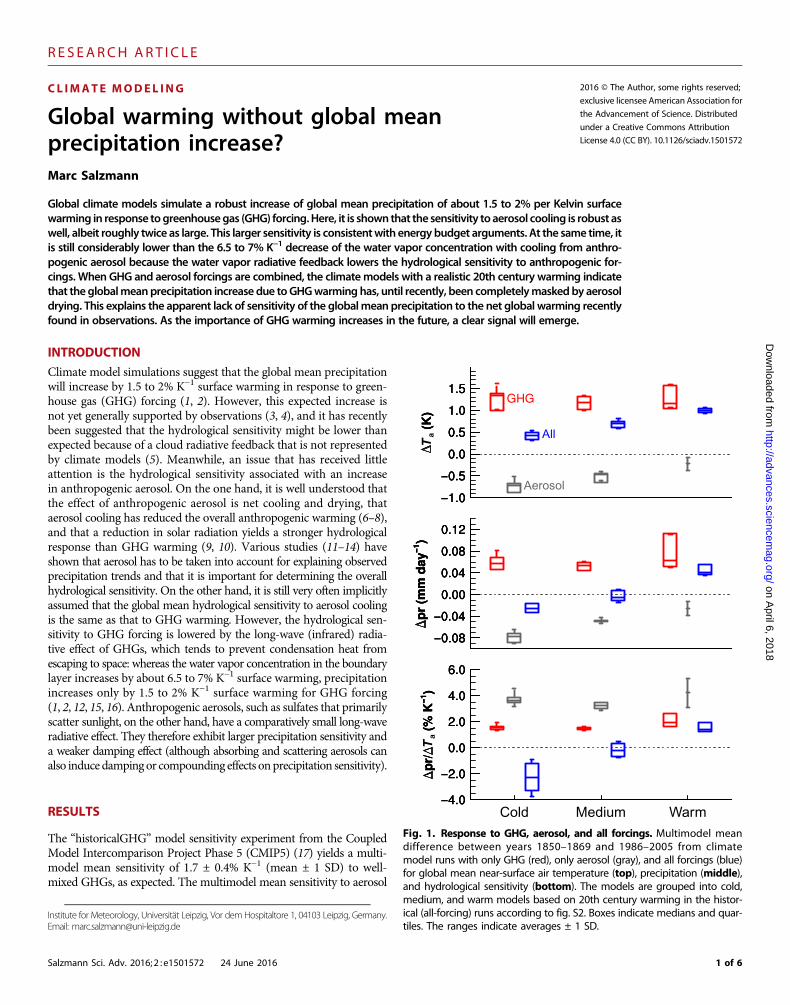
Fig. 1. Response to GHG, aerosol, and all forcings. Multimodel meandifference between years 1850–1869 and 1986–2005 from climatemodel runs with only GHG (red), only aerosol (gray), and all forcings (blue)for global mean near-surface air temperature (top), precipitation (middle),and hydrological sensitivity (bottom). The models are grouped into cold,medium, and warm models based on 20th century warming in the histor-ical (all-forcing) runs according to fig. S2. Boxes indicate medians and quar-tiles. The ranges indicate averages ± 1 SD.

1 of 6

R E S EARCH ART I C L E

on April 6, 2018

http://advances.sciencemag.org/

Dow

nloaded from

forcing, on the other hand, is roughly twice as large and also ratherrobust across different models (3.6 ± 0.5% K−1, based on eight CMIP5models for which aerosol-only runs are available; see the Supplemen-tary Materials for details). However, this sensitivity to aerosol coolingis still significantly lower than the 6.5 to 7% K−1 change of the lowertropospheric water vapor content, which is simulated in global climatemodels in response to surface temperature changes and which coin-cides with the expectations based on the Clausius-Clapeyron relation,under the assumption of constant relative humidity (2). Instead, it issimilar to the sensitivity that is obtained by comparing two CMIP5 ex-periments with fixed sea surface temperatures (SSTs), in one of whichthe SST is increased by 4 K everywhere (see table S1 and fig. S1) atconstant forcing, allowing only atmospheric feedbacks. This suggestsa significant contribution from the water vapor long-wave radiativefeedback and from long-wave cloud feedbacks to the overall damping,in agreement with previous studies (12, 13). The magnitude of thisdamping (roughly half the GHG damping) is compatible with the con-tribution of the water vapor feedback to the overall increased green-house effect [roughly a doubling (18)].

Here, the hydrological sensitivities have been estimated from differ-ences in surface air temperature DT and precipitation DP between theyears 1850–1869 and 1986–2005 from climate model runs with onlyGHG, only aerosol, and all forcings (Fig. 1), and the models have beengrouped according to the magnitude of their 20th century warming inthe all-forcing runs (fig. S2). Because the natural forcing is compar-atively small, DT and DP in the all-forcing runs are given by thesums of DT and DP from the GHG and aerosol runs, that is, DT =

Salzmann Sci. Adv. 2016; 2 : e1501572 24 June 2016

DTG + DTA and DP = DPG + DPA to a very good approximation(fig. S3). Consequently, the overall hydrological sensitivity can becomputed from

dPdT

¼ DPG þ DPADTG þ DTA

ð1Þ

which yields a rather accurate estimate according to fig. S3. Therefore,the global mean precipitation change is related to the individual hy-drological sensitivities as follows

DP ¼ dPdT

DT ¼ dPdT

� �G

DTG þ dPdT

� �A

DTA ð2Þ

where dPdT

� �Gand dP

dT

� �Aare the hydrological sensitivities from the

single-forcing experiments. Because DTG > 0 and DTA < 0 and alsodPdT

� �A> dP

dT

� �G, the actual (all-forcing) hydrological sensitivity is lower

than the known and often discussed sensitivity to GHGs (compareschematic in fig. S4). Overall, the simulated multimodel mean hydro-logical sensitivity is −0.4 ± 1.7% K−1 in the standard historical exper-iment that combines all forcings.

Figure 1 together with fig. S2 shows that the models that simulate afairly realistic 20th century warming (“medium”) tend to yield particu-larly small overall hydrological sensitivities, although it must be notedthat on average, themediummodels slightly underestimate the observedwarming, whereas the “warm”models yield several individual runs withonly a rather small overestimate of the global mean temperature in-crease. This suggests that the overall hydrological sensitivity is still much

A B

DC

Fig. 2. Regional precipitation response and additivity of responses to individual forcings. Multimodel averages of simulated surface precip-itation change between years 1850–1869 and 1986–2005 in millimeters per day for GHG, aerosol, and all forcings, as well as the sum of the GHG-and aerosol-forcing experiments for models for which at least one aerosol run is available. Stippling indicates that six of seven models (where twovery similar models have been considered as a single model) agree on the sign of the change.

2 of 6

R E S EARCH ART I C L E

on April 6, 2018

http://advances.sciencemag.org/

Dow

nloaded from

smaller than the hydrological sensitivity to GHGs and also still withinthe range of internal climate variability given by the spread between in-dividual model runs in fig. S3. It also explains the absence of a stronghydrological sensitivity in observations (4) and suggests that globalmean precipitation has not yet increased significantly despite globalwarming simply because the hydrological sensitivity to aerosol coolingis larger than that to GHG warming. This lack of observed response inglobal precipitation to GHG warming is consistent with energy budgetarguments and the analysis of historical trends in previous studies thathave taken into account aerosol effects (14, 16).

However, locally, the changes due to GHGs and aerosol do not bal-ance (Fig. 2 and figs. S5 to S7) because the aerosol forcing is highly non-uniform (19), which makes the detection of anthropogenic changespossible (20). Yet, to completely understand observed regional patternsofmultidecadal precipitation trends, onehas to take into account not onlyanthropogenic forcings but also internal climate variability (21–23). Al-though anthropogenic aerosol can have large influences on local circula-

Salzmann Sci. Adv. 2016; 2 : e1501572 24 June 2016

tion (24, 25), the overall effect on the global mean atmospheric verticaloverturning circulation strength ismuchweaker than that of GHGs (figs.S8 and S9). This is in line with the weaker damping and higher hydro-logical sensitivity, because the low sensitivity to GHG warming is asso-ciated with a weakening of the circulation under GHG warming (2).Ultimately, the local response of precipitation to anthropogenic forcingis determined not only by the temperature-dependent water vapor avail-ability and the strengthening or weakening of the overturning circulationbut also by geographical shifts of precipitation patterns (16). The impactsdepend strongly on changes of precipitation intensity (26, 27) and season-al cycle (28). Furthermore, the type of aerosol is important (11, 16, 29, 30),and also, the treatment of aerosol effects differs in global models (tableS2). This strongly influences the simulated changes in temperature andprecipitation. At the same time, the aerosol hydrological sensitivity isfound to be fairly robust (Fig. 1). Many features of the spatial patternssimulated in response to anthropogenic aerosol (Fig. 2B) are fairlyrobust as well (31), even across different models (figs. S5 to S7).

Because long-lived GHGs accumulate in the atmosphere while theatmospheric residence time of tropospheric aerosol is rather short, andbecause aerosol emissions are expected to decrease in the future, even-tually DTG will overwhelm DTA (32, 33), and thus the overall hydro-logical sensitivity will be dominated by GHGs. This is confirmed byanalyzing results from CMIP5 future scenario runs in Fig. 3.

DISCUSSION

The finding that the global mean hydrological response to aerosol isrobust across the models and independent of the exact treatment andstrength of the aerosol effect allows us to better understand simulatedand observed changes of the global mean hydrological cycle. Becausethe hydrological sensitivity in the CMIP5 historical coupledmodel runsdepends on the surface warming, the simulated hydrological sensitiv-ities can be constrained by surface temperature observations. This con-strained model-based estimate supports state-of-the-art observationalestimates (4), showing no evidence of a discernible historical trend. Fur-thermore, on the basis of the arguments above, one can see that if cli-mate geoengineering were used to reduce the global mean temperaturevia solar radiation management, the global mean precipitation in theresulting state would be reduced compared to what it would be at thesame temperature without the added GHGs, as suggested by Bala et al.(9), Bala et al. (10), and Bony et al. (15). On average, the precipitationdecrease would roughly correspond to the precipitation decrease thatis found when increasing the GHG concentrations in atmosphericmodels while keeping the SSTs fixed, although the geographical pat-tern would differ. This precipitation decrease has already been simu-lated in early uncoupledmodel simulations (1, 34). Conversely, reducedaerosol emissions help to “unmask” the precipitation increase by GHGwarming (35). Eventually, the global mean aerosol effect on precipita-tion will almost completely be overwhelmed by GHG warming asexpected on the basis of previous studies (32, 33, 36).

MATERIALS AND METHODS

Model data and analysis methodModel data were taken from the CMIP5 (17). In total, 282 atmosphere-oceancoupledmodel runs from15CMIP5modelsand24atmosphere-only

Cold Medium Warm

aa

.Fig. 3. Future projections. Similar to Fig. 1 but showing differences be-tween years 2006–2025 and 2081–2100 based on the rcp45 (brown) and

the rcp85 (purple) CMIP5 future emission scenarios.

3 of 6

R E S EARCH ART I C L E

on April 6, 2018

http://advances.sciencemag.org/

Dow

nloaded from

runs from 11 CMIP5 models were analyzed. For the coupled modelruns, only runs frommodels that have performed at least one so-calledsingle-forcing experiment in addition to the standard CMIP5 historicalexperiment were taken into account [as in the work by Salzmann et al.(25); see Table 1 and tables S2 to S4 for an overview]. In particular, thehistoricalGHG experiment takes into account only the forcing by well-mixed anthropogenicGHGs, whereas several runs from theCMIP5his-toricalMisc collection of experiments included only the forcing bychanging anthropogenic aerosol concentrations. Only natural forcingswere included in the historicalNat runs, with the two main natural for-cings being volcanic aerosol and solar variability. These single-forcingexperiments facilitated the calculation of changes with respect to a givenforcing, that is, the change of a climate variable, such as surface tem-perature or precipitation due to this particular forcing when all otherforcings are kept constant. However, although the other forcings werekept constant, water vapor and clouds were still allowed to respond tothe single forcing, so that these changes are not the same as partial de-rivatives. The single forcingswere abbreviated “GHG” for anthropogen-ic GHG, “aerosol” for anthropogenic aerosol, and “nat” for naturalforcings. In addition to these single-forcing runs, runs from the standardhistorical experiment were analyzed. This experiment took into account

Salzmann Sci. Adv. 2016; 2 : e1501572 24 June 2016

all the known anthropogenic GHG and aerosol, as well as natural forc-ings. The experiment was abbreviated “all.”The historical runs typicallystart in 1850 and end in 2005, and the differences between the first andthe last 20 years were analyzed as in the study by Held and Soden (2),except when the runs were compared to observations. Then, the years1901–1920 were compared to the years 1986–2005. Uncertainties andintermodel spread in the CMIP5 historical coupled model runs stemfrom uncertainty in simulated aerosol radiative forcing, cloud radiativefeedback strength, and ocean heat uptake.

Furthermore, two runs from two experiments with prescribed SSTswere analyzed. In these amip-style runs (where amip originally standsfor Atmospheric Model Intercomparison Project), all radiative forcingswere taken into account, but the SSTs could not react. Instead, observation-derived SSTs for the years 1979–2005 were prescribed in the standardamip run. In the amip4K run, the prescribed SSTs were increased by4K everywhere, but the forcings remained identical to those in theamip base run. From the difference between the global time averages,one could then compute a hydrological sensitivity for constant forcing,allowing only feedbacks. All years of the two amip runs were takeninto account. The results from amip runs should, in general, be treatedwith caution because at the lower boundary, energy is not conserved.

Table 1. Models. CNRM, Centre National de Recherches Météorologiques; CERFACS, Centre Européen de Recherche et de Formation Avancée enCalcul Scientifique; CSIRO, Australian Commonwealth Scientific and Industrial Research Organisation, in collaboration with the Queensland ClimateChange Centre of Excellence; LASG, State Key Laboratory Numerical Modeling for atmospheric Sciences and geophysical Fluid Dynamics; IAP, In-stitute of Atmospheric Physics of the Chinese Academy of Sciences; CESS, Center for Earth System Science, Tshinghua University; FIO, First Instituteof Oceanography, State Oceanic Administration; NOAA, National Oceanic and Atmospheric Administration; NASA, National Aeronautics and SpaceAdministration; JAMSTEC, Japan Agency for Marine-Earth Science and Technology; AORI, Atmosphere and Ocean Research Institute, The Universityof Tokyo; NIES, National Institute for Environmental Studies, Ibaraki, Japan.

Model

Center Reference

bcc-csm1-1

Beijing Climate Center (40)

CanESM2/CanAM4

Canadian Centre for Climate Modelling and Analysis (41)

CCSM4

National Center for Atmospheric Research (42)

CNRM-CM5

CNRM-CM5 CNRM and CERFACS (43)

CSIRO-Mk3-6-0

CSIRO Marine and Atmospheric Research (44)

FGOALS-g2

LASG, IAP, CESS, and FIO (45)

GFDL-CM3

NOAA Geophysical Fluid Dynamics Laboratory (46)

GFDL-ESM2

NOAA Geophysical Fluid Dynamics Laboratory (47)

GISS-E2-H

NASA Goddard Institute for Space Studies (48)

GISS-E2-R

NASA Goddard Institute for Space Studies (48)

HadGEM2-ES

Met Office Hadley Centre (49)

IPSL-CM5A-LR

Institut Pierre Simon Laplace (50)

MIROC-ESM

JAMSTEC, AORI, and NIES (51)

MIROC-ESM-CHEM

JAMSTEC, AORI, and NIES (51)

MIROC5

JAMSTEC, AORI, and NIES (52)

MRI-CGCM3

Meteorological Research Institute, Tsukuba, Japan (53)

MPI-ESM-LR

Max Planck Institute for Meteorology (54)

NorESM1-M

Norwegian Climate Centre (55)

4 of 6

R E S EARCH ART I C L E

on April 6, 2018

http://advances.sciencemag.org/

Dow

nloaded from

Global averages were computed from the original data, whereas formaps, the model output has been regridded to a 2° × 2° grid. The termmultimodel average refers to an average in which initially all the realiza-tions (runs with slightly different initial conditions) from a given modelare averaged before averaging over the models. In the maps showingmodel averages, the runs from the twoNASAGoddard Institute for SpaceStudies (GISS)modelswere combined into one before averaging, whereasotherwise they were considered separately. The data analysis was per-formed using freely available software (see Acknowledgments).

Observational dataFor model evaluation purposes, SSTs from the NOAA Extended Re-constructed Sea Surface Temperature (ERSST) version 4 (37) werecombined with 2° × 2° regridded near-surface air temperature datafrom the Climatic Research Unit Time Series, version 3.22 (CRUTS3.22) data set (38), which is based on the work by Mitchell andJones (39). While processing the data, a mask based on the maximumsea ice extent from the ERSST data set was used to mask out regionsthat could potentially be influenced by sea ice. This approach ofmasking out the maximum ice extent has been chosen to accountfor the fact that the CMIP5 experiments analyzed here are not deter-ministic with respect to internal variability [see, for example, the studyby Salzmann and Cherian (23)].

These observation-derived surface temperatures are used to constrainhydrological sensitivity based on atmosphere-ocean coupled climatemodel simulations. An alternative method that provides additional in-sights is an energy budget analysis along the lines of previous work byAndrews et al. (11), Previdi (12), O’Gorman et al. (13), Wu et al. (14),and Allan et al. (16). However, unfortunately, the uncertainties asso-ciated with observational estimates of the surface energy budget thatcould help to constrain the coupled models’ energy budgets with ob-servations are rather large.

SUPPLEMENTARY MATERIALSSupplementary material for this article is available at http://advances.sciencemag.org/cgi/content/full/2/6/e1501572/DC1Notes regarding selected figuresfig. S1. Hydrological sensitivity for fixed SST.fig. S2. Grouping of models according to 20th century temperature increase.fig. S3. Response to GHG, aerosol, and all forcings from individual models.fig. S4. Schematic representation of the hydrological sensitivity to various forcings.fig. S5. Zonal mean precipitation change from individual models.fig. S6. Maps of surface precipitation change from individual models (part1).fig. S7. Maps of surface precipitation change from individual models (part2).fig. S8. Global mean atmospheric overturning circulation changes for GHG, aerosol, and all forcings.fig. S9. As fig. S8 for individual model runs.table S1. Hydrological sensitivity (% K−1).table S2. Treatment of indirect (cloud-aerosol) radiative effects in the historical runs.table S3. CMIP5 experiments used in this study.table S4. Number of runs per model used in this study.Reference (56)

REFERENCES AND NOTES1. M. R. Allen, W. J. Ingram, Constraints on future changes in climate and the hydrologic

cycle. Nature 419, 224–232 (2002).2. I. M. Held, B. J. Soden, Robust responses of the hydrological cycle to global warming.

J. Climate 19, 5686–5699 (2006).3. V. O. John, R. P. Allan, B. J. Soden, How robust are observed and simulated precipitation

responses to tropical ocean warming? Geophys. Res. Lett. 36, L14702 (2009).4. G. Gu, R. F. Adler, Spatial patterns of global precipitation change and variability during

1901-2010. J. Climate 28, 4431–4453 (2015).

Salzmann Sci. Adv. 2016; 2 : e1501572 24 June 2016

5. T. Mauritsen, B. Stevens, Missing iris effect as a possible cause of muted hydrologicalchange and high climate sensitivity in models. Nat. Geosci. 8, 346–351 (2015).

6. J. F. B. Mitchell, T. C. Johns, On modification of global warming by sulfate aerosols. J. Climate10, 245–267 (1997).

7. U. Lohmann, J. Feichter, Global indirect aerosol effects: A review. Atmos. Chem. Phys. 5,715–737 (2005).

8. G. Myhre, D. Shindell, F.-M. Bréon, W. Collins, J. Fuglestvedt, J. Huang, D. Koch, J.-F. Lamarque,D. Lee, B. Mendoza, T. Nakajima, A. Robock, G. Stephens, T. Takemura, H. Zhang, ClimateChange 2013: The Physical Science Basis. Contribution of Working Group I to the Fifth AssessmentReport of the Intergovernmental Panel on Climate Change, T. F. Stocker, D. Qin, G.-K. Plattner,M. Tignor, S. K. Allen, J. Boschung, A. Nauels, Y. Xia, V. Bex, P. M. Midgley, Eds. (Cambridge Univ.Press, Cambridge and New York, 2013).

9. G. Bala, P. B. Duffy, K. E. Taylor, Impact of geoengineering schemes on the global hydro-logical cycle. Proc. Natl. Acad. Sci. U.S.A. 105, 7664–7669 (2008).

10. G. Bala, K. Caldeira, R. Nemani, L. Cao, G. G. Ban-Weiss, H.-J. Shin, Albedo enhancement of marineclouds to counteract global warming: Impacts on the hydrological cycle. Clim. Dynam. 37,915–931 (2011).

11. T. Andrews, P. M. Forster, O. Boucher, N. Bellouin, A. Jones, Precipitation, radiative forcingand global temperature change. Geophys. Res. Lett. 37, L14701, (2010).

12. M. Previdi, Radiative feedbacks on global precipitation. Env. Res. Lett. 5, 025211 (2010).13. P. A. O’Gorman, R. P. Allan, M. P. Byrne, M. Previdi, Energetic constraints on precipitation

under climate change. Surv. Geophys. 33, 585–608 (2012).14. P. Wu, N. Christidis, P. Stott, Anthropogenic impact on Earth’s hydrological cycle. Nat. Clim.

Change 3, 807–810 (2013).15. S. Bony, G. Bellon, D. Klocke, S. Sherwood, S. Fermepin, S. Denvil, Robust direct effect of

carbon dioxide on tropical circulation and regional precipitation. Nat. Geosci. 6, 447–451 (2013).16. R. P. Allan, C. Liu, M. Zahn, D. A. Lavers, E. Koukouvagias, A. Bodas-Salcedo, Physically

consistent responses of the global atmospheric hydrological cycle in models and observa-tions. Surv. Geophys. 35, 533–552 (2014).

17. K. E. Taylor, R. J. Stouffer, G. A. Meehl, An overview of CMIP5 and the experiment design.Bull. Am. Meteorol. Soc. 93, 485–498 (2012).

18. I. M. Held, B. J. Soden, Water vapor feedback and global warming. Annu. Rev. Energy Environ25, 441–475 (2000).

19. S. Kinne, D. O’Donnel, P. Stier, S. Kloster, K. Zhang, H. Schmidt, S. Rast, M. Giorgetta,T. F. Eck, B. Stevens, Mac-v1: A new global aerosol climatology for climate studies.J. Adv. Model. Earth Syst. 5, 704–740 (2013).

20. X. Zhang, F. W. Zwiers, G. C. Hegerl, F. H. Lambert, N. P. Gillett, S. Solomon, P. A. Stott, T. Nozawa,Detection of human influence on twentieth-century precipitation trends. Nature 448, 461–465(2007).

21. A. Saha, S. Ghosh, A. S. Sahana, E. P. Rao, Failure of CMIP5 climate models in simulatingpost-1950 decreasing trend of Indian monsoon. Geophys. Res. Lett. 41, 7323–7330 (2014).

22. L. Krishnamurthy, V. Krishnamurthy, Decadal scale oscillations and trend in the Indianmonsoon rainfall. Clim. Dynam. 43, 319–331 (2014).

23. M. Salzmann, R. Cherian, On the enhancement of the indian summer monsoon drying byPacific multidecadal variability during the latter half of the twentieth century. J. Geophys.Res. Atmos. 120, 9103–9118 (2015).

24. M. A. Bollasina, Y. Ming, V. Ramaswamy, Anthropogenic aerosols and the weakening of theSouth Asian summer monsoon. Science 334, 502–505 (2011).

25. M. Salzmann, H. Weser, R. Cherian, Robust response of Asian summer monsoon to anthro-pogenic aerosols in CMIP5 models. J. Geophys. Res. Atmos. 119, 11321–11337 (2014).

26. K. E. Trenberth, Changes in precipitation with climate change. Clim. Res. 47, 123–138 (2011).27. J. Lehmann, D. Coumou, K. Frieler, Increased record-breaking precipitation events under

global warming. Clim. Change 132, 501–515 (2015).28. J. G. Dwyer, M. Biasutti, A. H. Sobel, The effect of greenhouse gas–induced changes in SST

on the annual cycle of zonal mean tropical precipitation. J. Climate 27, 4544–4565 (2014).29. Y. Ming, V. Ramaswamy, G. Persad, Two opposing effects of absorbing aerosols on global

mean precipitation. Geophys. Res. Lett. 37, L13701 (2010).30. C. Wang, Impact of anthropogenic absorbing aerosols on clouds and precipitation: A re-

view of recent progresses. Atmos. Res. 122, 237–249 (2013).31. M. M. Kvalevoåg, B. H. Samset, G. Myhre, Hydrological sensitivity to greenhouse gases and

aerosols in a global climate model. Geophys. Res. Lett. 40, 1432–1438 (2013).32. J.-L. Dufresne, J. Quaas, O. Boucher, S. Denvil, L. Fairhead, Contrasts in the effects on cli-

mate of anthropogenic sulfate aerosols between the 20th and the 21st century. Geophys.Res. Lett. 32, L21703 (2005).

33. G. Myhre, O. Boucher, F.-M. Bréon, P. Forster, D. Shindell, Declining uncertainty in transient cli-mate response as CO2 forcing dominates future climate change. Nat. Geosci. 8, 181–185 (2015).

34. J. F. B. Mitchell, The seasonal response of a general circulation model to changes in CO2

and sea temperatures. Q. J. Roy. Meteorol. Soc. 109, 113–152 (1983).35. H. Levy II, L. W. Horowitz, M. D. Schwarzkopf, Y. Ming, J.-C. Golaz, V. Naik, V. Ramaswamy,

The roles of aerosol direct and indirect effects in past and future climate change. J. Geophys.Res. Atmos. 118, 4521–4532 (2013).

5 of 6

R E S EARCH ART I C L E

on April 6, 2018

http://advances.sciencemag.org/

Dow

nloaded from

36. S. J. Smith, T. C. Bond, Two hundred fifty years of aerosols and climate: The end of the ageof aerosols. Atmos. Chem. Phys. 14, 537–549 (2014).

37. B. Huang, V. F. Banzon, E. Freeman, J. Lawrimore, W. Liu, T. C. Peterson, T. M. Smith,P.W. Thorne, S. D. Woodruff, H.-M. Zhang, Extended reconstructed sea surface temperatureversion 4 (ERSST.v4). Part I: Upgrades and intercomparisons. J. Climate 28, 911–930 (2015).

38. I. Harris, P. D. Jones, University of East Anglia Climatic Research Unit, CRU TS3.22: ClimaticResearch Unit (CRU) Time-Series (TS) Version 3.22 of high resolution gridded data ofmonth-by-month variation in climate (Jan. 1901-Dec. 2013), NCAS British AtmosphericData Centre, 24 September 2014.

39. T. D. Mitchell, P. D. Jones, An improved method of constructing a database of monthly climateobservations and associated high-resolution grids. Int. J. Climatology 25, 693–712 (2005).

40. T. Wu, R. Yu, F. Zhang, Z. Wang, M. Dong, L. Wang, X. Jin, D. Chen, L. Li, The Beijing ClimateCenter atmospheric general circulation model: Description and its performance for thepresent-day climate. Clim. Dynam. 34, 123–147 (2010).

41. V. K. Arora, J. F. Scinocca, G. J. Boer, J. R. Christian, K. L. Denman, G. M. Flato, V. V. Kharin,W. G. Lee, W. J. Merryfield, Carbon emission limits required to satisfy future representativeconcentration pathways of greenhouse gases. Geophys. Res. Lett. 38, L05805 (2011).

42. P. R. Gent, G. Danabasoglu, L. J. Donner, M. M. Holland, E. C. Hunke, S. R. Jayne,D. M. Lawrence, R. B. Neale, P. J. Rasch, M. Vertenstein, P. H. Worley, Z.-L. Yang,M. Zhang, The Community Climate System Model Version 4. J. Climate 24, 4973–4991 (2011).

43. A. Voldoire, E. Sanchez-Gomez, D. Salas y Mélia, B. Decharme, C. Cassou, S. Sénési, S. Valcke,I. Beau, A. Alias, M. Chevallier, M. Déqué, J. Deshayes, H. Douville, E. Fernandez, G. Madec,E. Maisonnave, M.-P. Moine, S. Planton, D. Saint-Martin, S. Szopa, S. Tyteca, R. Alkama,S. Belamari, A. Braun, L. Coquart, F. Chauvin, The CNRM-CM5.1 global climate model: Descrip-tion and basic evaluation. Clim. Dynam. 40, 2091–2121 (2013).

44. L. D. Rotstayn, S. J. Jeffrey, M. A. Collier, S. M. Dravitzki, A. C. Hirst, J. I. Syktus, K. K. Wong, Aerosol-and greenhouse gas-induced changes in summer rainfall and circulation in the Australasianregion: A study using single-forcing climate simulations. Atmos. Chem. Phys. 12, 6377–6404 (2012).

45. L. Li, P. Lin, Y. Yu, B. Wang, T. Zhou, L. Liu, J. Liu, Q. Bao, S. Xu, W. Huang, K. Xia, Y. Pu,L. Dong, S. Shen, Y. Liu, N. Hu, M. Liu,W. Sun, X. Shi,W. Zheng, B. Wu, M. Song, H. Liu,X. Zhang, G. Wu,W. Xue, X. Huang, G. Yang, Z. Song, F. Qiao, The flexible global ocean-atmo-sphere-land system model, grid-point version 2: FGOALS-g2. Adv. Atmos. Sci. 30, 543–560 (2013).

46. L. J. Donner, B. L. Wyman, R. S. Hemler, L. W. Horowitz, Y. Ming, M. Zhao, J.-C. Golaz,P. Ginoux, S.-J. Lin, M. D. Schwarzkopf, J. Austin, G. Alaka, W. F. Cooke, T. L. Delworth,S. M. Freidenreich, C. T. Gordon, S. M. Griffies, I. M. Held, W. J. Hurlin, S. A. Klein,T. R. Knutson, A. R. Langenhorst, H.-C. Lee, Y. Lin, B. I. Magi, S. L. Malyshev, P. C. D. Milly,V. Naik, M. J. Nath, R. Pincus, J. J. Ploshay, V. Ramaswamy, C. J. Seman, E. Shevliakova,J. J. Sirutis, W. F. Stern, R. J. Stouffer, R. J. Wilson, M. Winton, A. T. Wittenberg, F. Zeng, The dy-namical core, physical parameterizations, and basic simulation characteristics of the atmosphericcomponent AM3 of the GFDL global coupled model CM3. J. Climate 24, 3484–3519 (2011).

47. J. P. Dunne, J. G. John, A. J. Adcroft, S. M. Griffies, R. W. Hallberg, E. Shevliakova,R. J. Stouffer, W. Cooke, K. A. Dunne, M. J. Harrison, J. P. Krasting, S. L. Malyshev,P. C. D. Milly, P. J. Phillipps, L. T. Sentman, B. L. Samuels, M. J. Spelman, M. Winton,A. T. Wittenberg, N. Zadeh, GFDLs ESM2 global coupled climate–carbon earth systemmodels. Part I: Physical formulation and baseline simulation characteristics. J. Climate25, 6646–6665 (2012).

48. G. A. Schmidt, M. Kelley, L. Nazarenko, R. Ruedy, G. L. Russell, I. Aleinov, M. Bauer,S. E. Bauer, M. K. Bhat, R. Bleck, V. Canuto, Y.-H. Chen, Y. Cheng, T. L. Clune,A. Del Genio, R. de Fainchtein, G. Faluvegi, J. E. Hansen, R. J. Healy, N. Y. Kiang, D. Koch,A. A. Lacis, A. N. LeGrande, J. Lerner, K. K. Lo, E. E. Matthews, S. Menon, R. L. Miller, V. Oinas,A. O. Oloso, J. P. Perlwitz, M. J. Puma, W. M. Putman, D. Rind, A. Romanou, M. Sato,D. T. Shindell, S. Sun, R. A. Syed, N. Tausnev, K. Tsigaridis, N. Unger, A. Voulgarakis,M.-S. Yao, J. Zhang, Configuration and assessment of the GISS ModelE2 contributions tothe CMIP5 archive. J. Adv. Model. Earth Syst. 6, 141–184 (2014).

49. G. M. Martin, N. Bellouin, W. J. Collins, I. D. Culverwell, P. R. Halloran, S. C. Hardiman,J. Hinton, C. D. Jones, R. E. McDonald, A. J. McLaren, F. M. O’Connor, M. J. Roberts,J. M. Rodriguez, S. Woodward, M. J. Best, M. E. Brooks, A. R. Brown, N. Butchart,C. Dearden, S. H. Derbyshire, I. Dharssi, M. Doutriaux-Boucher, J. M. Edwards, P. D. Falloon,N. Gedney, L. J. Gray, H. T. Hewitt, M. Hobson, M. R. Huddleston, J. Hughes, S. Ineson,W. J. Ingram, P. M. James, T. C. Johns, C. E. Johnson, A. Jones, C. P. Jones, M. M. Joshi,A. B. Keen, S. Liddicoat, A. P. Lock, A. V. Maidens, J. C. Manners, S. F. Milton, J. G. L. Rae,J. K. Ridley, A. Sellar, C. A. Senior, I. J. Totterdell, A. Verhoef, P. L. Vidale, A. Wiltshire, TheHadGEM2 family of met office unified model climate configurations. Geosci. Model Dev. 4,723–757 (2011).

50. J.-L. Dufresne, M.-A. Foujols, S. Denvil, A. Caubel, O. Marti, O. Aumont, Y. Balkanski, S. Bekki,H. Bellenger, R. Benshila, S. Bony, L. Bopp, P. Braconnot, P. Brockmann, P. Cadule, F. Cheruy,F. Codron, A. Cozic, D. Cugnet, N. de Noblet, J.-P. Duvel, C. Ethé, L. Fairhead, T. Fichefet,

Salzmann Sci. Adv. 2016; 2 : e1501572 24 June 2016

S. Flavoni, P. Friedlingstein, J.-Y. Grandpeix, L. Guez, E. Guilyardi, D. Hauglustaine,F. Hourdin, A. Idelkadi, J. Ghattas, S. Joussaume, M. Kageyama, G. Krinner, S. Labetoulle,A. Lahellec, M.-P. Lefebvre, F. Lefevre, C. Levy, Z. X. Li, J. Lloyd, F. Lott, G. Madec, M. Mancip,M. Marchand, S. Masson, Y. Meurdesoif, J. Mignot, I. Musat, S. Parouty, J. Polcher, C. Rio,M. Schulz, D. Swingedouw, S. Szopa, C. Talandier, P. Terray, N. Viovy, N. Vuichard, Climatechange projections using the IPSL-CM5 Earth System Model: from CMIP3 to CMIP5. Clim.Dynam. 40, 2123–2165 (2013).

51. S. Watanabe, T. Hajima, K. Sudo, T. Nagashima, T. Takemura, H. Okajima, T. Nozawa,H. Kawase, M. Abe, T. Yokohata, T. Ise, H. Sato, E. Kato, K. Takata, S. Emori, M. Kawamiya,MIROC-ESM 2010: Model description and basic results of CMIP5-20c3m experiments. Geosci.Model Dev. 4, 845–872 (2011).

52. M. Watanabe, T. Suzuki, R. O’ishi, Y. Komuro, S. Watanabe, S. Emori, T. Takemura, M. Chikira,T. Ogura, M. Sekiguchi, K. Takata, D. Yamazaki, T. Yokohata, T. Nozawa, H. Hasumi,H. Tatebe, M. Kimoto, Improved climate simulation by MIROC5. Mean states, variability,and climate sensitivity. J. Climate 23, 6312–6335 (2010).

53. S. Yukimoto, Y. Adachi, M. Hosaka, T. Sakami, H. Yoshimura, M. Hirabara, T. Y. Tanaka,E. Shindo, H. Tsujino, M. Deushi, R. Mizuta, S. Yabu, A. Obata, H. Nakano, T. Koshiro, T. Ose,A. Kitoh, A new global climate model of the meteorological research institute: MRICGCM3–Model description and basic performance. J. Meteor. Soc. Japan 90A, 23–64 (2012).

54. M. A. Giorgetta, J. Jungclaus, C. H. Reick, S. Legutke, J. Bader, M. Böttinger, V. Brovkin,T. Crueger, M. Esch, K. Fieg, K. Glushak, V. Gayler, H. Haak, H.-D. Hollweg, T. Ilyina,S. Kinne, L. Kornblueh, D. Matei, T. Mauritsen, U. Mikolajewicz, W. Mueller, D. Notz,F. Pithan, T. Raddatz, S. Rast, R. Redler, E. Roeckner, H. Schmidt, R. Schnur,J. Segschneider, K. D. Six, M. Stockhause, C. Timmreck, J. Wegner, H. Widmann,K.-H. Wieners, M. Claussen, J. Marotzke, B. Stevens, Climate and carbon cycle changes from1850 to 2100 in MPI-ESM simulations for the Coupled Model Intercomparison Projectphase 5. J. Adv. Model. Earth Syst. 5, 572–597 (2013).

55. M. Bentsen, I. Bethke, J. B. Debernard, T. Iversen, A. Kirkevåg, Ø. Seland, H. Drange,C. Roelandt, I. A. Seierstad, C. Hoose, J. E. Kristjánsson, The Norwegian Earth System Model,NorESM1-M – Part 1: Description and basic evaluation of the physical climate. Geosci.Model Dev. 6, 687–720 (2013).

56. J.-C. Golaz, L. W. Horowitz, H. Levy II, Cloud tuning in a coupled climate model: Impact on20th century warming. Geophys. Res. Lett. 40, 2246–2251 (2013).

Acknowledgments: I thank the climate modeling groups (Table 1) for producing and makingavailable their model output, the data distribution centers, and the World Climate ResearchProgramme’s Working Group on Coupled Modelling, which is responsible for CMIP5. Severalcolleagues, especially J. Quaas and J. Mülmenstädt, and two anonymous reviewers havecontributed useful comments. The NCAR (National Center for Atmospheric Research) Com-mand Language (version 6.3.0) [Software]. (2015), Boulder, Colorado: UCAR/NCAR/CISL/TDD,http://dx.doi.org/10.5065/D6WD3XH5 has been used for data analysis and visualization. Cli-mate data operators developed at the Max Planck Institute for Meteorology in Hamburg havealso been used for data processing. The software for distributing the data was developed bythe U.S. Department of Energy’s Program for Climate Model Diagnosis and Intercomparison inpartnership with the Global Organization for Earth System Science Portals. Funding: This workhas been supported by the Universität Leipzig and European Research Council grant “QUAERERE”(grant agreement no. 306284). I thank the German Reserach foundation (DFG) and UniversitätLeipzig for support within the program for Open Access Publishing. Competing interests: The au-thor declares that he has no competing interests. Data andmaterials availability: Coupled modeloutput data have been obtained via Earth System Grid Federation servers (for example, https://pcmdi.llnl.gov/projects/esgf-llnl/). Data from amip-style runs have been obtained from the CERA(Climate and Environmental Retrieval and Archive) gateway at the DKRZ (German Climate Com-puting Center) in Hamburg (http://cera-www.dkrz.de/CERA/), where also CMIP5 coupled modeloutput can be downloaded. CMIP5 data can also be downloaded from the Natural EnvironmentResearch Council’s British Atmospheric Data Centre at http://badc.nerc.ac.uk/home/. The ERSSTdata can be obtained from www1.ncdc.noaa.gov/pub/data/cmb/ersst/v4/netcdf/. The CRU dataare available at http://dx.doi.org/10.5285/18BE23F8-D252-482D-8AF9-5D6A2D40990C. All dataneeded to evaluate the conclusions in the paper are present in the paper and/or the Supplemen-tary Materials. Additional data related to this paper may be requested from the authors.

Submitted 4 November 2015Accepted 31 May 2016Published 24 June 201610.1126/sciadv.1501572

Citation: M. Salzmann, Global warming without global mean precipitation increase?. Sci. Adv.2, e1501572 (2016).

6 of 6

Global warming without global mean precipitation increase?Marc Salzmann

DOI: 10.1126/sciadv.1501572 (6), e1501572.2Sci Adv 

ARTICLE TOOLS http://advances.sciencemag.org/content/2/6/e1501572

MATERIALSSUPPLEMENTARY http://advances.sciencemag.org/content/suppl/2016/06/21/2.6.e1501572.DC1

REFERENCES

http://advances.sciencemag.org/content/2/6/e1501572#BIBLThis article cites 54 articles, 2 of which you can access for free

PERMISSIONS http://www.sciencemag.org/help/reprints-and-permissions

Terms of ServiceUse of this article is subject to the

registered trademark of AAAS.is aScience Advances Association for the Advancement of Science. No claim to original U.S. Government Works. The title

York Avenue NW, Washington, DC 20005. 2017 © The Authors, some rights reserved; exclusive licensee American (ISSN 2375-2548) is published by the American Association for the Advancement of Science, 1200 NewScience Advances

on April 6, 2018

http://advances.sciencemag.org/

Dow

nloaded from