global warming - rice universityfew/global warming revised.pdf · the global average temperature...

Arthur FewProfessor Emeritus, Research Professor

Physics and AstronomyRice University

Global Warming

I have been lecturing on this subject to my classes for 39 years, so this lecture was condensed from my course lectures and updated with the most current information.

My point of view is most certainly that of the scientific community - that global warming is real, it is happening now and will continue into the future, and that the distractors of global warming fail to (or do not wish to) understand the fundamental science of global warming.

In this current form of the lecture I have added voiceover to the slides. The commentary is synchronized with the slides; when the audio stops the slides will automatically advance to the next slide.

You can pause the slide show at any time using the “f” key (for freeze); to restart use any key.

Part 1:General discussion of temperature and warming, and why there is a disconnect between the scientist and the nonscientist.

Part 2:The science of global warming, this is how it works.

Do We Understand Temperature?

What is the temperature of this room?

Where would you measure the temperature of this room?

How would you measure the temperature?!When do you measure the temperature of the room?

Can we call this measurement the “average” room temperature?

We have illustrated some complexities in the meaning of temperature. Temperature is a point measurement, and when applied to an extended object, we must agree on the specifics of where, how, and when to make a consensus “room temperature” measurement. Beyond this we must also reach a consensus on what averages we want to know.


So, what is the temperature of the Earth?

Where do we place the thermometers?!

How do you average these spatially diverse measurements?

How long should the record be to give a significant average measurement?!

Difficult as it might be there are experts that labor over the global data set and carefully weigh the quality and distribution of the data to achieve the mean global temperature and its changes over time. These are peer reviewed and become consensus determinations. The following slide provides a summary of the many attempts to determine the global temperature.

I recommend that you pause the next slide after the commentary is finished and study the slides details.


I think there is a more convincing way to measure global warming; that is to let the Earth do the averaging for us. We can observe changes in glaciers. Changes in sea ice, land ice , and snow cover. Changes in insect populations. Changes in soil moisture. Changes in vegetation. These and many other Earth System components respond to changes in climate.

Before we examine some of these Earth-integrated observed changes let’s look at another obstacle in the communication between the scientist and the nonscientists.

In order to make any sense out of global temperature data sets, the measurements must be “massaged”- calibrated, adjusted, smoothed, averaged, etc. This is not an easy task, but once this is done with historical data, new data sets can be added using the consensus methodology.

Do We Understand Warming?

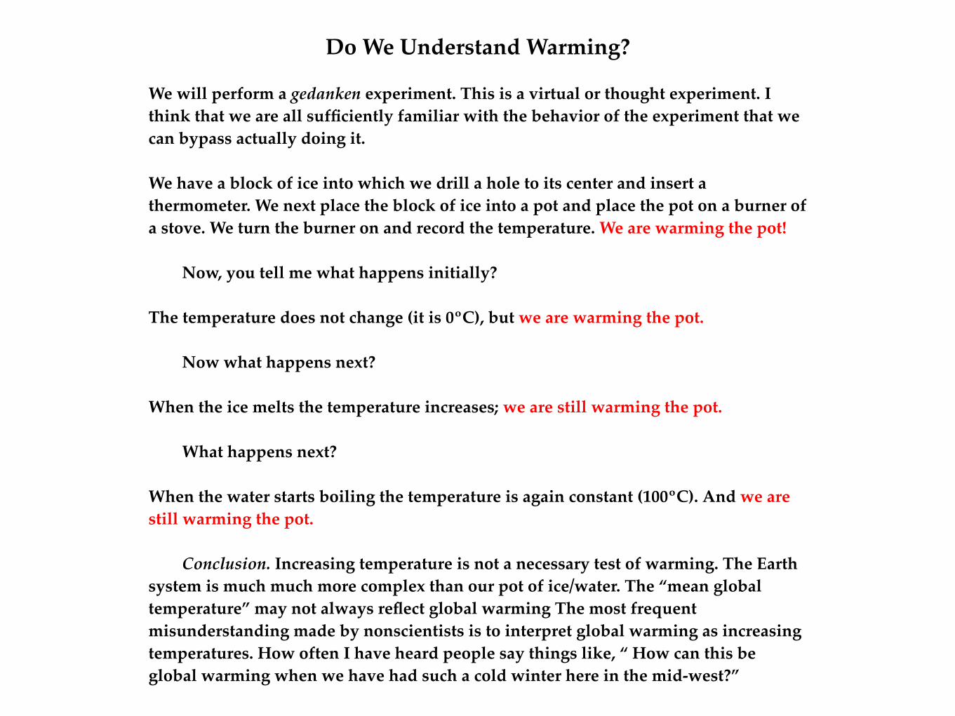
We will perform a gedanken experiment. This is a virtual or thought experiment. I think that we are all sufficiently familiar with the behavior of the experiment that we can bypass actually doing it.

We have a block of ice into which we drill a hole to its center and insert a thermometer. We next place the block of ice into a pot and place the pot on a burner of a stove. We turn the burner on and record the temperature. We are warming the pot!

! Now, you tell me what happens initially?

The temperature does not change (it is 0ºC), but we are warming the pot.

! Now what happens next?

When the ice melts the temperature increases; we are still warming the pot.

! What happens next?

When the water starts boiling the temperature is again constant (100ºC). And we are still warming the pot.

! Conclusion. Increasing temperature is not a necessary test of warming. The Earth system is much much more complex than our pot of ice/water. The “mean global temperature” may not always reflect global warming The most frequent misunderstanding made by nonscientists is to interpret global warming as increasing temperatures. How often I have heard people say things like, “ How can this be global warming when we have had such a cold winter here in the mid-west?”

In my opinion, the scientific community made a mistake decades ago when trying to convince the general public of the dangers of global warming by focusing upon global temperature. It simply doesn’t convey the proper message.

Suppose you tell your Houston business persons that by 2020 the global average temperature will increase by 1ºC. What probably goes through their mind is, “Gosh, will I be able to play golf in January?”

The global average temperature does not properly convey the real message of global warming, and may, in fact, be misleading to the general public.

Take this example: the oceans have a hugh heat capacity compared to the atmosphere and land (the part that interacts with weather and climate changes). For a 1ºC change in the “global average temperature” the oceans might change by 0.2ºC while the land change would be 3ºC. I can assure you the increasing our average mid-continent land temperature 3ºC will lead to droughts and extensive agriculture failures.

The scientific community has now realized the importance of forecasting regional impacts of global warming and pointing to the observed changes that are already taking place.

Some Observed Consequences of Global Warming(IPCC Report AR4, November 2007, and AR3, September 2001)

Eleven of the last twelve years (1995-2006) rank among the twelve warmest years in the instrumental record of global surface temperature (since 1850).

Rising sea level is consistent with warming.

Observed decreases in snow and ice extent are also consistent with warming. Arctic sea ice extent has shrunk by ~3% per decade, with larger decreases in summer of ~7% per decade.

It is very likely that over the past 50 years: cold days, cold nights and frosts have become less frequent over most land areas, and hot days and hot nights have become more frequent.

There is observational evidence of an increase in intense tropical cyclone activity in the North Atlantic since about 1970.

Average Northern Hemisphere temperatures during the second half of the 20th century were very likely higher than during any other 50-year period in the last 500 years and likely the highest in at least the past 1300 years.

Changes in snow, ice and frozen ground have with high confidence increased the number and size of glacial lakes, increased ground instability in mountain and other permafrost regions and led to changes in some Arctic and Antarctic ecosystems.

In terrestrial ecosystems, earlier timing of spring events and poleward and upward shifts in plant and animal ranges are with very high confidence linked to recent warming.

There has been a widespread retreat of mountain glaciers in non-polar regions during the 20th century.

It is likely that there has been about a 40% decline in Arctic sea-ice thickness during late summer to early autumn in recent decades and a considerably slower decline in winter sea-ice thickness.

Tide gauge data show that global average sea level rose between 0.1 and 0.2 meters during the 20th century.

Warm episodes of the El Niño-Southern Oscillation (ENSO) phenomenon (which consistently affects regional variations of precipitation and temperature over much of the tropics, sub-tropics and some mid-latitude areas) have been more frequent, persistent and intense since the mid-1970s, compared with the previous 100 years.

Ocean waters are becoming more acidic as they soak up carbon dioxide, the main global warming gas. And while there's evidence that coral reefs can find ways to adapt to waters warmed by global climate change, there's no proof that they can cope with more-acidic oceans. But a new research paper in the journal Science says their problems may be getting worse. The paper says as much as a third of the world's coral species may now be headed toward extinction.

Climate change is "largely irreversible" for the next 1,000 years even if carbon dioxide (CO2) emissions could be abruptly halted, according to a new study published in this week's Proceedings of the National Academy of Sciences (1/29/09). This is because the oceans are currently soaking up a lot of the planet's excess heat — and a lot of the carbon dioxide put into the air. The carbon dioxide and heat will eventually start coming out of the ocean. And that will take place for many hundreds of years.

Some Personal Observations.

Drunken Trees

Missing Glacier(Turnagain Arm & Portage Glacier; also Glacier National Park and Kilimanjaro)

Grosbeaks & Crossbeaks

House Finches

Yellowjackets

Pine Bark Beetles(Entomologist say 4 consecutive days Of -10ºF required to kill a beetle larva.)

Ips Bark Beetle

Gulf Coast HurricanesIke, Gustav, Dolly, Humberto, Dean, Ernesto, Cindy, Dennis, Emily, Katrina, Rita, Stan, Wilma, Beta, 2005 used up the alphabet then switched to Greek - alpha through zeta.

Wildfires

Earthʼs Effective Temperature

σTE4 , Stefan–Boltzmann law

σ = 5.67x10-8 J/sm2K4

S = 1366 J/sm2 dS = 0.07%A = 0.30 (28 - 30)

Power In = S(1-A)πRE2



σ = 5.67x10-8 J/sm2K4

S = 1366 J/sm2 dS = 0.07%A = 0.30 (28 - 30)

Power In = S(1-A)πRE2 Power Out = 4πRE2 σTE4



σ = 5.67x10-8 J/sm2K4

S = 1366 J/sm2 dS = 0.07%A = 0.30 (28 - 30)


TE = [S(1-A)/4σ]1/4



σ = 5.67x10-8 J/sm2K4

S = 1366 J/sm2 dS = 0.07%A = 0.30 (28 - 30)

TE = 255ºK = -18ºCThat’s Cold!


TE = [S(1-A)/4σ]1/4



σ = 5.67x10-8 J/sm2K4

S = 1366 J/sm2 dS = 0.07%A = 0.30 (28 - 30)

Also, the global mean includes the polar regions. By the way, the tropical cloud tops are colder than the polar regions.

17% ofIR out


17% ofIR out

83% ofIR out


17% ofIR out

83% ofIR out

When viewing the Earth from space in the infrared, you see mostly the atmosphere and clouds; the surface contributes but a small fraction. The

atmosphere and clouds are much colder than the surface.


17% ofIR out

83% ofIR out

When viewing the Earth from space in the infrared, you see mostly the atmosphere and clouds; the surface contributes but a small fraction. The

atmosphere and clouds are much colder than the surface.

This component is the albedo.72% is from the atmosphere.

28% is from the surface.


10 Introduction and Overview

Solution: Solving Eq. (1.9), we obtain z ! H ln (p0!p),and similarly for density. Hence, the heights are (a)

for the 1-kg m"3 density level and (b)

for the 1-hPa pressure level. Because H varies withheight, geographical location, and time, and the refer-ence values #0 and p0 also vary, these estimates areaccurate only to within "10%. !

Exercise 1.4 Assuming an exponential pressureand density dependence, calculate the fraction of thetotal mass of the atmosphere that resides between 0and 1 scale height, 1 and 2 scale heights, 2 and 3 scaleheights, and so on above the surface.

Solution: Proceeding as in Exercise 1.2, the fractionof the mass of the atmosphere that lies between 0 and1, 1 and 2, 2 and 3, and so on scale heights abovethe Earth’s surface is e"1, e"2, . . . e"N from which itfollows that the fractions of the mass that reside inthe 1st, 2nd . . ., Nth scale height above the surface are1 " e"1, e"1(1 " e"1), e"2(1 " e"1) . . ., e"N(1 " e"1),where N is the height of the base of the layer expressedin scale heights above the surface. The correspondingnumerical values are 0.632, 0.233, 0.086 . . . !

Throughout most of the atmosphere the concen-trations of N2, O2, Ar, CO2, and other long-lived con-stituents tend to be quite uniform and largelyindependent of height due to mixing by turbulentfluid motions.7 Above "105 km, where the mean freepath between molecular collisions exceeds 1 m(Fig. 1.8), individual molecules are sufficiently mobilethat each molecular species behaves as if it alonewere present. Under these conditions, concentrationsof heavier constituents decrease more rapidly withheight than those of lighter constituents: the densityof each constituent drops off exponentially with

7.5 km $ ln #10001.00$ ! 52 km

7.5 km $ ln #1.251.00$ ! 1.7 km

height, with a scale height inversely proportional tomolecular weight, as explained in Section 3.2.2. Theupper layer of the atmosphere in which the lightermolecular species become increasingly abundant (ina relative sense) with increasing height is referred toas the heterosphere. The upper limit of the lower,well-mixed regime is referred to as the turbopause,where turbo refers to turbulent fluid motions andpause connotes limit of.

The composition of the outermost reaches of theatmosphere is dominated by the lightest molecularspecies (H, H2, and He). During periods when thesun is active, a very small fraction of the hydrogenatoms above 500 km acquire velocities high enoughto enable them to escape from the Earth’s gravita-tional field during the long intervals between molec-ular collisions. Over the lifetime of the Earth theleakage of hydrogen atoms has profoundly influ-enced the chemical makeup of the Earth system, asdiscussed in Section 2.4.1.

The vertical distribution of temperature for typi-cal conditions in the Earth’s atmosphere, shown inFig. 1.9, provides a basis for dividing the atmos-phere into four layers (troposphere, stratosphere,

7 In contrast, water vapor tends to be concentrated within the lowest few kilometers of the atmosphere because it condenses and pre-cipitates out when air is lifted. Ozone are other highly reactive trace species exhibit heterogeneous distributions because they do notremain in the atmosphere long enough to become well mixed.

0

10

20

30

40

50

60

90

100

160 180 200 220 240 260 280 300Temperature (K)

Hei

ght (

km)

1000

100

10

1

0.1

0.01

0.001

300

80

70

Pre

ssur

e (h

Pa)

Thermosphere

Mesopause

Mesosphere

Stratopause

Stratosphere

TroposphereTropopause

Fig. 1.9 A typical midlatitude vertical temperature profile,as represented by the U.S. Standard Atmosphere.

P732951-Ch01.qxd 9/12/05 7:38 PM Page 10

255ºK

~ 1/2 Atmospheric Mass

This is how it works.a(0-1) = absorbtivity = emissivity (Kirchhoff’s Law): the fraction of the total radiation that is absorbed or emitted.Earth now: a = 0.766 close to the upper limit for a 1-layer atmosphere.

The atmosphereis depicted as alayer above the Earth’s surface.



Most of the solarradiation that is not

reflected (albedo) passes though the

atmosphere and warms the Earth’s surface.






The warm surfaceradiates infrared

radiation upward.







radiation upward.

A small fraction of the surface radiationpasses through the

atmosphere to space.







radiation upward.



Most of the surface radiation is absorbed

in the atmosphere and warms the

atmosphere.







radiation upward.





atmosphere.

The warmed atmosphere radiatesupward to space and

downward to the surface.







radiation upward.





atmosphere.

The warmed atmosphere radiatesupward to space and

downward to the surface.

The final result of this interaction of the atmosphere with the upward and downward radiation is that the surface is warmed by both the Sun and the

atmosphere. This is global warming. When the greenhouse gasses increase, the warming increases - the law of radiation transfer. This result is unavoidable.


122 Radiative Transfer

(F units of solar radiation plus F units of longwaveradiation emitted by the upper layer). To balance theincident radiation, the lower layer must emit 2F unitsof longwave radiation. Because the layer is isother-mal, it also emits 2F units of radiation in the down-ward radiation. Hence, the downward radiation atthe surface of the planet is F units of incident solarradiation plus 2F units of longwave radiation emittedfrom the atmosphere, a total of 3F units, which mustbe balanced by an upward emission of 3F units oflongwave radiation from the surface. !

By induction, the aforementioned analysis can beextended to an N-layer atmosphere. The emissionsfrom the atmospheric layers, working downwardfrom the top, are F, 2F, 3F . . . NF and the correspon-ding radiative equilibrium temperatures are 255, 303,335 . . . . [(N ! 1)F!"]1!4 K. The geometric thicknessof opaque layers decreases approximately exponen-tially as one descends through the atmosphere due tothe increasing density of the absorbing medium withdepth. Hence, the radiative equilibrium lapse ratesteepens with increasing depth. In effect, radiativetransfer becomes less and less efficient at removingthe energy absorbed at the surface of the planet dueto the increasing blocking effect of greenhouse gases.Once the radiative equilibrium lapse rate exceeds theadiabatic lapse rate (Eq. 3.53), convection becomesthe primary mode of energy transfer.

That the global mean surface temperature of theEarth is 289 K rather than the equivalent blackbodytemperature 255 K, as calculated in Exercise 4.6, is

attributable to the greenhouse effect. Were it not forthe upward transfer of latent and sensible heat byfluid motions within the Earth’s atmosphere, the dis-parity would be even larger.

To perform more realistic radiative transfer calcu-lations, it will be necessary to consider the depend-ence of absorptivity upon the wavelength of theradiation. It is evident from the bottom part ofFig. 4.7 that the wavelength dependence is quite pro-nounced, with well-defined absorption bands identi-fied with specific gaseous constituents, interspersedwith windows in which the atmosphere is relativelytransparent. As shown in the next section, the wave-length dependence of the absorptivity is even morecomplicated than the transmissivity spectra in Fig. 4.7would lead us to believe.

4.4 Physics of Scatteringand Absorption and EmissionThe scattering and absorption of radiation by gasmolecules and aerosols all contribute to the extinc-tion of the solar and terrestrial radiation passingthrough the atmosphere. Each of these contributionsis linearly proportional to (1) the intensity of theradiation at that point along the ray path, (2) thelocal concentration of the gases and/or particlesthat are responsible for the absorption and scatter-ing, and (3) the effectiveness of the absorbers orscatterers.

Let us consider the fate of a beam of radiationpassing through an arbitrarily thin layer of theatmosphere along a specific path, as depicted in Fig.4.10. For each kind of gas molecule and particle thatthe beam encounters, its monochromatic intensity isdecreased by the increment

(4.16)

where N is the number of particles per unit volumeof air, " is the areal cross section of each particle,K# is the (dimensionless) scattering or absorptionefficiency, and ds is the differential path lengthalong the ray path of the incident radiation. Anextinction efficiency, which represents the combinedeffects of scattering and absorption in depleting theintensity of radiation passing through the layer, canbe defined in a similar manner. In the case of agaseous atmospheric constituent, it is sometimes

dI# $ %I#K#N"ds

F

F

F 3F

2F

2F

F

F

Fig. 4.9 Radiation balance for a planetary atmosphere that istransparent to solar radiation and consists of two isothermallayers that are opaque to planetary radiation. Thin downwardarrows represent the flux of F units of shortwave solar radiationtransmitted downward through the atmosphere. Thicker arrowsrepresent the emission of longwave radiation from the surfaceof the planet and from each of the layers. For radiative equilib-rium the net radiation passing through the Earth’s surface andthe top of each of the layers must be equal to zero.

P732951-Ch04.qxd 9/12/05 7:41 PM Page 122

Simplified greenhouse model of two internally isothermal atmospheric layers but with different temperatures. The upward and downward fluxes at each level must be equal. Start at the top level; one F down must be matched by one F up. Each layer must radiate the same flux down that it radiates up; thus the top layer radiates one F down. Now there are two Fs down into the bottom layer, which must be matched by two Fs up and down. This makes three Fs down to the surface, which must radiate three Fs up. The temperature must increase downward because the lower layers must radiate more flux than the higher layers.

Venus: A=0.75 TE=232KEarth: A=0.30 TE= 255KVenus: TS=737KEarth: TS= 288KGreenhouse V = 505K( or C)Greenhouse E = 33K (or C)Using the simple model on this slide for Venus requires 19 layers of atmospheres!

The next step is to use a multilevel model for an atmosphere. Current large numerical models for Earth use at least 15 layers. Consider the 2-layer model here.

122 Radiative Transfer

(F units of solar radiation plus F units of longwaveradiation emitted by the upper layer). To balance theincident radiation, the lower layer must emit 2F unitsof longwave radiation. Because the layer is isother-mal, it also emits 2F units of radiation in the down-ward radiation. Hence, the downward radiation atthe surface of the planet is F units of incident solarradiation plus 2F units of longwave radiation emittedfrom the atmosphere, a total of 3F units, which mustbe balanced by an upward emission of 3F units oflongwave radiation from the surface. !

By induction, the aforementioned analysis can beextended to an N-layer atmosphere. The emissionsfrom the atmospheric layers, working downwardfrom the top, are F, 2F, 3F . . . NF and the correspon-ding radiative equilibrium temperatures are 255, 303,335 . . . . [(N ! 1)F!"]1!4 K. The geometric thicknessof opaque layers decreases approximately exponen-tially as one descends through the atmosphere due tothe increasing density of the absorbing medium withdepth. Hence, the radiative equilibrium lapse ratesteepens with increasing depth. In effect, radiativetransfer becomes less and less efficient at removingthe energy absorbed at the surface of the planet dueto the increasing blocking effect of greenhouse gases.Once the radiative equilibrium lapse rate exceeds theadiabatic lapse rate (Eq. 3.53), convection becomesthe primary mode of energy transfer.

That the global mean surface temperature of theEarth is 289 K rather than the equivalent blackbodytemperature 255 K, as calculated in Exercise 4.6, is

attributable to the greenhouse effect. Were it not forthe upward transfer of latent and sensible heat byfluid motions within the Earth’s atmosphere, the dis-parity would be even larger.

To perform more realistic radiative transfer calcu-lations, it will be necessary to consider the depend-ence of absorptivity upon the wavelength of theradiation. It is evident from the bottom part ofFig. 4.7 that the wavelength dependence is quite pro-nounced, with well-defined absorption bands identi-fied with specific gaseous constituents, interspersedwith windows in which the atmosphere is relativelytransparent. As shown in the next section, the wave-length dependence of the absorptivity is even morecomplicated than the transmissivity spectra in Fig. 4.7would lead us to believe.

4.4 Physics of Scatteringand Absorption and EmissionThe scattering and absorption of radiation by gasmolecules and aerosols all contribute to the extinc-tion of the solar and terrestrial radiation passingthrough the atmosphere. Each of these contributionsis linearly proportional to (1) the intensity of theradiation at that point along the ray path, (2) thelocal concentration of the gases and/or particlesthat are responsible for the absorption and scatter-ing, and (3) the effectiveness of the absorbers orscatterers.

Let us consider the fate of a beam of radiationpassing through an arbitrarily thin layer of theatmosphere along a specific path, as depicted in Fig.4.10. For each kind of gas molecule and particle thatthe beam encounters, its monochromatic intensity isdecreased by the increment

(4.16)

where N is the number of particles per unit volumeof air, " is the areal cross section of each particle,K# is the (dimensionless) scattering or absorptionefficiency, and ds is the differential path lengthalong the ray path of the incident radiation. Anextinction efficiency, which represents the combinedeffects of scattering and absorption in depleting theintensity of radiation passing through the layer, canbe defined in a similar manner. In the case of agaseous atmospheric constituent, it is sometimes

dI# $ %I#K#N"ds

F

F

F 3F

2F

2F

F

F

Fig. 4.9 Radiation balance for a planetary atmosphere that istransparent to solar radiation and consists of two isothermallayers that are opaque to planetary radiation. Thin downwardarrows represent the flux of F units of shortwave solar radiationtransmitted downward through the atmosphere. Thicker arrowsrepresent the emission of longwave radiation from the surfaceof the planet and from each of the layers. For radiative equilib-rium the net radiation passing through the Earth’s surface andthe top of each of the layers must be equal to zero.

P732951-Ch04.qxd 9/12/05 7:41 PM Page 122

Simplified greenhouse model of two internally isothermal atmospheric layers but with different temperatures. The upward and downward fluxes at each level must be equal. Start at the top level; one F down must be matched by one F up. Each layer must radiate the same flux down that it radiates up; thus the top layer radiates one F down. Now there are two Fs down into the bottom layer, which must be matched by two Fs up and down. This makes three Fs down to the surface, which must radiate three Fs up. The temperature must increase downward because the lower layers must radiate more flux than the higher layers.

In this model of surface warming, adding greenhouse gasses is analogous to adding layers to this model.

Venus: A=0.75 TE=232KEarth: A=0.30 TE= 255KVenus: TS=737KEarth: TS= 288KGreenhouse V = 505K( or C)Greenhouse E = 33K (or C)Using the simple model on this slide for Venus requires 19 layers of atmospheres!

The next step is to use a multilevel model for an atmosphere. Current large numerical models for Earth use at least 15 layers. Consider the 2-layer model here.

Primarily visible 100 units in. Visible 28, Infrared 72

100 units out.

Radiation energy transfer in the Earth system;short wave (visible) and long wave (infrared).

UV radiationabsorbed by O3


Near IR radiationabsorbed by H2O,

dust, haze & pollution.




Visible sunlight directlyabsorbed by the surface.





Visible sunlight scattered in the atmosphere and absorbed by the surface. Clouds 14, Air 11.





Visible sunlight scattered in the atmosphere and absorbed by the surface. Clouds 14, Air 11.

Visible sunlight scattered or reflected back to space = Albedo.

Clouds 19, Air 6, Surface 3

When the Earth is viewed from space in visible radiation,we mostly see clouds (19 units, white)

and air (6 units, blue);least is the surface (3 units, various colors).

These arrows indicate energy transport by

winds and currents not by radiation

These arrows represent energy transport by air flow, but they are very important to the energy balance between the surface and the atmosphere.

Upward IR emission from stratosphere = downward

absorption in visible


absorption in visibleIR upward emission =

solar absorption inthe stratosphere



Of the 114 units of IR radiated upward from the surface, 5 units pass through the atmosphere to space while 109 units are absorbed by the atmosphere. Sensible

heat and latent heat add 29 units of upward energy into the atmosphere.

IR upward emission =solar absorption inthe stratosphere



Upward IR emission from the atmosphere & clouds







72 = 3 + 5 + 64







72 = 3 + 5 + 64

Downward IRAtmosphere to surface.




When the Earth is viewed from space in infrared radiation,we mostly see air and clouds (67 units),

and a small surface contribution (5 units).

The downward IR radiation from the atmosphere (96 units) is larger than the downward solar radiation (47 units) by a factor more than 2.

Note the following:

More solar radiation arrives at the surface after atmospheric scattering processes (25 units) than by direct sunlight (22).

Energy balance at the surface is only achieved when sensible and latent heats are included.Solar in 22 + 25 = 47

IR in 96IR out -114; Sensible and Latent out -29; Total out = -143

Net = -47

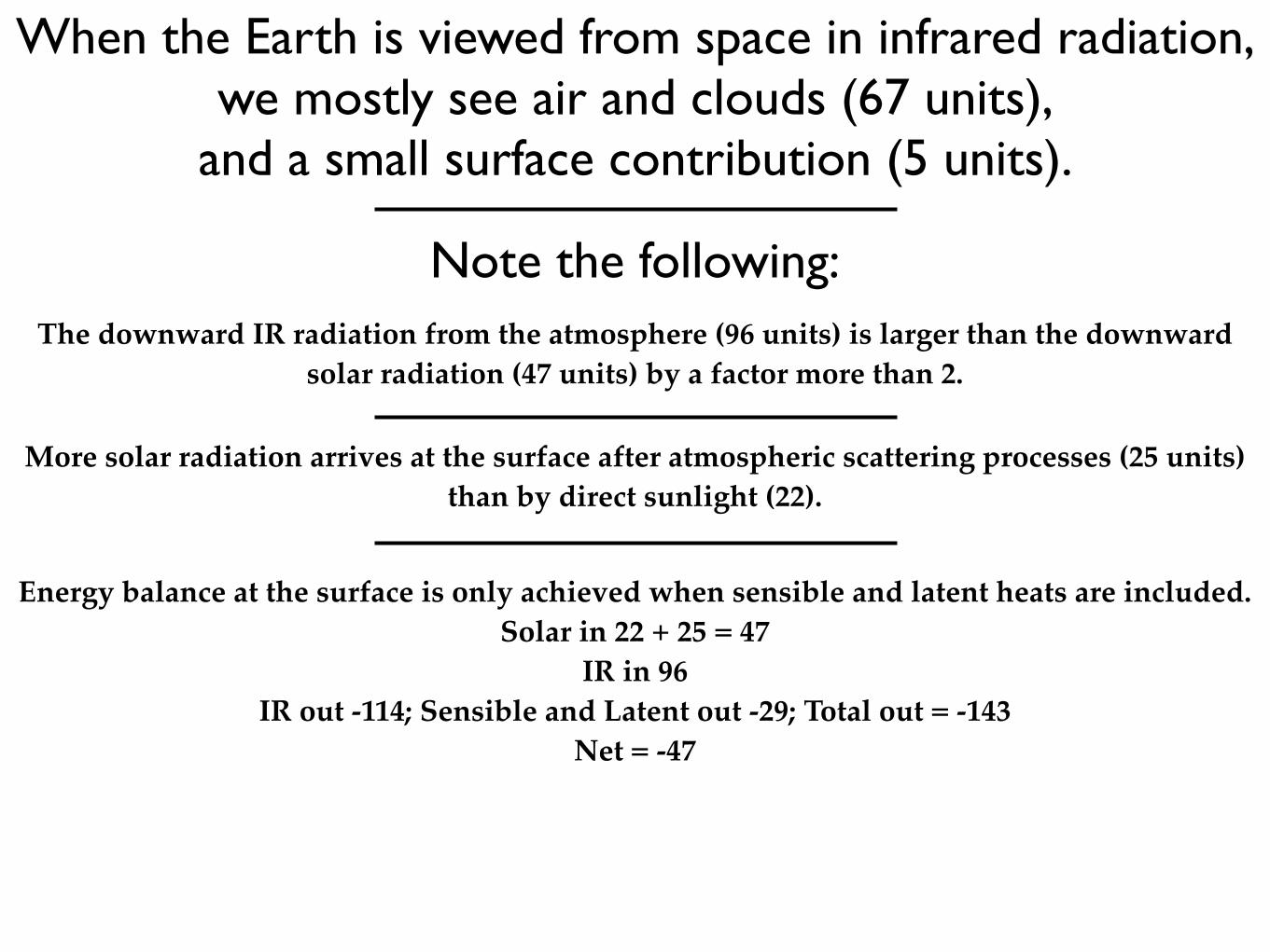
When the Earth is viewed from space in infrared radiation,we mostly see air and clouds (67 units),

and a small surface contribution (5 units).

The downward IR radiation from the atmosphere (96 units) is larger than the downward solar radiation (47 units) by a factor more than 2.

Note the following:

More solar radiation arrives at the surface after atmospheric scattering processes (25 units) than by direct sunlight (22).

Energy balance at the surface is only achieved when sensible and latent heats are included.Solar in 22 + 25 = 47

IR in 96IR out -114; Sensible and Latent out -29; Total out = -143

Net = -47

Energy Balance








7.5 km $ ln #10001.00$ ! 52 km

7.5 km $ ln #1.251.00$ ! 1.7 km





0

10

20

30

40

50

60

90

100

160 180 200 220 240 260 280 300Temperature (K)

Hei

ght (

km)

1000

100

10

1

0.1

0.01

0.001

300

80

70

Pre

ssur

e (h

Pa)

Thermosphere

Mesopause

Mesosphere

Stratopause

Stratosphere



P732951-Ch01.qxd 9/12/05 7:38 PM Page 10

255ºK









7.5 km $ ln #10001.00$ ! 52 km

7.5 km $ ln #1.251.00$ ! 1.7 km





0

10

20

30

40

50

60

90

100

160 180 200 220 240 260 280 300Temperature (K)

Hei

ght (

km)

1000

100

10

1

0.1

0.01

0.001

300

80

70

Pre

ssur

e (h

Pa)

Thermosphere

Mesopause

Mesosphere

Stratopause

Stratosphere



P732951-Ch01.qxd 9/12/05 7:38 PM Page 10

255ºK


The rapid decrease in temperature with

altitude in the troposphere results

primarily from convection. When the

surface is warmed, convection is

enhanced and the upper troposphere

gets colder.

~100 years

~10 years

~1 year

~1 day

~100 years

~10 years

~1 year

~1 day

Compare

~100 years

~10 years

~1 year

~1 day

Not shown is water vapor, a strong greenhouse gas; the lifetime for water vapor in

the atmosphere is 7-10 days. Although a natural

atmospheric component evaporation increases with surface warming; this is a positive feedback process

that responds to carbon dioxide increases.

Compare

Two important greenhouse gasses for the past 440 years; CO2 and CH4.

Carbon dioxide is the primary villain!

What has changed?

What has changed?

This is what we have added!

What has changed?

This is what we have added!

The Earth has not experienced this level of CO2 in the last 440 thousand years; other ice cores go back 650 thousand and show the same result.

-0.3ºC

-0.3ºC

+0.3ºC

-0.3ºC

+0.3ºC0.6ºC

warmingThis is not

very convincing.

The “hockey stick” curve; sea level has

the same shape.

-0.3ºC

+0.3ºC0.6ºC

warmingThis is not

very convincing.

Natural: volcanos, solar

Anthropogenic: greenhouse gasses, pollution, land use

The modeling is improving

IPCC, 1990

IPCC, 1996

IPCC, 2001

38 ppm

23 yrs

1.7 ppm/yr

38 ppm

23 yrs

1.7 ppm/yr

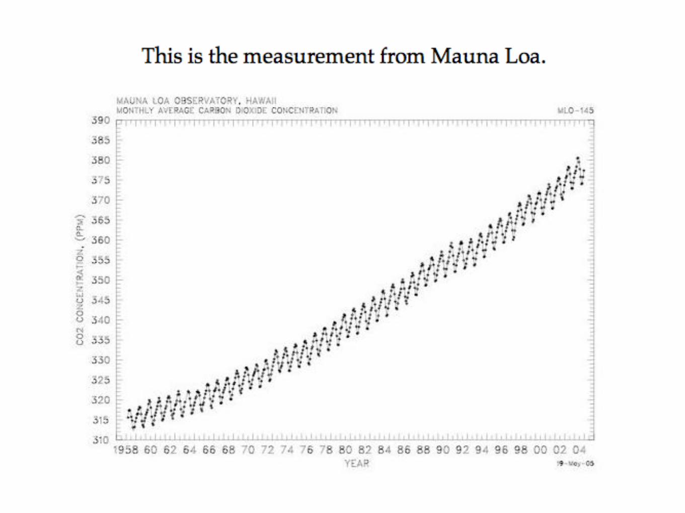
Annual variation in the Northern Hemisphere CO2.Land plants photosynthesis

and respiration; peak occurs in NH summer.

~9 ppm/yr

From IPCC 2001

Ocean Exchange+105-107

Vegetation Loss +2

Soils +60

Land Plants+60-120

Fossil Fuels +5

Net to Atmosphere +5

From Schlesinger 1991Simplified using only the most active exchanges; no very long time scale exchanges.

Small quantitative differences.

2001 IPCC: 5.5 Gt/yr2007 IPCC: 7 Gt/yr

We can create a simple computer model using STELLA to test the carbon cycle as given.


0.1

0.4

105

107


5

2

?

107

105

6060

120


60.4

0.4

60

60

120


This routine introduces seasonal variations into the

photosynthesis rate


This computation converts Gt to ppm

Net 46 yr increase in atmospheric CO2

If all of our carbon emissions stayed in the atmosphere the

CO2 would exceed the measured amount.

The previous result with Unknown Sink = 0

Setting the Unknown Sink to 2 Gt/yr improves the model

output, but we are still not in agreement with measurements.



output, but we are still not in agreement with measurements.


Our “Net carbon to the atmosphere” was 5 Gt/yr; yet with an unknown sink = 2 Gt/yr we are not yet matching the measurement. What are we missing?

Temporarily ignore the red curve.


The previous results with Unknown Sink = 0

Unknown Sink = 2



Unknown Sink = 2


output, but we are still not in agreement with measurements. Note the large deviation from the measurements in the last

half of the model run.


Unknown Sink = 2





Unknown Sink = 2




On this model run we have also displayed the carbon in the Land Plants, which we now see is decreasing significantly because of deforestation.

When Land Plants decrease, the photosynthesis also decreases and a major natural carbon sink decreases, so the Unknown Sink = 4 is insufficient.


Unknown Sink = 2Unknown Sink = 4

Hypothesis. Deforestation seems to be inconsistent with the CO2 measurements. What if the “Unknown Sink” is going into enhanced forest growth to compensate for the deforestation?

This next model run sets Unknown Sink = 0 and “Deforestation” = -0.5, a small net gain.The previous results with Unknown Sink = 0





Setting the Unknown Sink to 0 and the Deforestation = -0.5 Gt/yr

to represent a net increase in Land Plants produces agreement

with measurements. This is called CO2 fertilization, but it

also represents natural recovery from previous deforestation.




Setting the Unknown Sink to 0 and the Deforestation = -0.5 Gt/yr

to represent a net increase in Land Plants produces agreement

with measurements. This is called CO2 fertilization, but it

also represents natural recovery from previous deforestation.

This is a very simple modeling exercise, but it can provide powerful insights into how the Earth system interacts with human perturbations.

• Greenhouse gasses warm the Earth’s surface. Increasing greenhouse gasses increases the warming. This is a consequence of the Laws of Radiation Transfer and is unavoidable.• Humankind’s emissions of greenhouse gasses have increased the atmospheric load of these gasses beyond anything the Earth has experienced in 650,000 years. • The Earth’s global temperature is very difficult to determine; temperature is influenced by other processes in the Earth system, and the range of temperature change is so small (< 1ºC) that it is an unconvincing parameter to use for public discussions. Sea level rise is only slightly better.• More convincing evidence of global warming is available from changes in the Earth system that integrate the impacts of surface warming such as glaciers, ice sheets, sea ice, snow cover, ecological changes, etc. All of these measures point to a warming Earth.• Humanity is currently emitting 7 Gt C/yr (fourteen trillion (14,000,000,000,000) pounds per

year) into the atmosphere. The Earth can only handle half that quantity at best; the rest is accumulating in the atmosphere and is producing observable greenhouse warming of the Earth’s surface.• The way that the Earth is dealing with this part CO2 overload is in increased forest growth and over saturation of oceanic CO2. Eventually, the oceans will release its excess CO2 back into the atmosphere, and the new forest growth will mature and no longer be a sink for CO2.

Summary

So, what do we do?• The usual litany: energy conservation, renewable energy, etc. These will help and are good directions to move, but they are insufficient - too little, too late, but necessary.• More oil and gas production: This is the wrong direction but unavoidable.• Nuclear: Probably unavoidable - very expensive.• Geoengineering:(1)Fertilizing the oceans - probably won’t work.(2)Seeding clouds - questionable and expensive.(3)Sequestering CO2 underground - questionable reservoirs and expensive.(4)Sequestering CO2 on the ocean bottom - dangerous and expensive.

My suggestion.• Listen to what the Earth is telling us. Put it in the oceans and forests.• Ocean storage is temporary and acidifying the ecosystem.• Reforestation and afforestation is also temporary unless managed continuously. Mature trees must be cut and and used so as to remove the wood from the decay cycle. (1)Pulped wood will return to the atmosphere in short time.(2)Construction wood will be sequestered for much longer time.(3)Wood used for energy can displace fossil fuel thus is a permanent reduction in released CO2.

The figure shows cumulative carbon-stock changes for a scenario involving afforestation and harvest for a mix of traditional forest products with some of the harvest being used as a fuel. Values are illustrative of what might be observed in the southeastern USA or Central Europe. Regrowth restores carbon to the forest and the (hypothetical) forest stand is harvested every 40 years, with some litter left on the ground to decay, and products accumulate or are disposed of in landfills. These are net changes in that, for example, the diagram shows savings in fossil fuel emissions with respect to an alternative scenario that uses fossil fuels and alternative, more energy-intensive products to provide the same services.

Soil

Litter

Trees

Long-lived products

Short-lived products

Landfill

Energy for products

Displaced fossil fuels

Time (years)

Cum

ulat

ive

carb

on

global warming - rice universityfew/global warming revised.pdf · the global average temperature...

Documents