Global WarmingA Zonal Energy Balance Model

Victor Padron

Normandale Community College

MATHEMATICAL FIELD

Calculus and Differential Equations.

APPLICATION FIELD

Climate Models and Environmental Science.

TARGET AUDIENCE

Students in an elementary mathematical modeling course or in a course of calculus

with elementary differential equations, including numerical solutions for systems

of ordinary differential equations.

ABSTRACT

Global warming is a response of the Earth to an imbalance between the energy

absorbed and emitted by the planet. Earth is currently out of balance because

increasing atmospheric greenhouse gases such as CO2 reduce the planet’s heat ra-

diation to space, thus causing an energy imbalance. This imbalance causes Earth

to warm in order to restore the energy balance. A Zonal Energy Balance Model

(ZEBM) that tracks Earth’s northern hemisphere temperatures is derived. Stu-

dents working with this module will write a computer code to obtain numerical

solutions of ZEBM, and will play the role of an environmental analyst by devising

strategies for reduction of the growth of rate atmospheric CO2 concentration in

order to avoid “dangerous levels” of global warming.

PREREQUISITES

Precalculus and basic programing skills.

TECHNOLOGY

Access to a computer algebra system, such as Mathematica or MATLAB, is re-

quired for the main activities of this modulus.

AKNOWLEDGMENTS

This teaching module was created for Engaging Mathematics with support from the

National Science Foundation under grant DUE-1322883 to the National Center for

Science and Civic Engagement. An initiative of the National Center for Science and

Civic Engagement, Engaging Mathematics applies the well-established SENCER

method to college level mathematics courses, with the goal of using civic issues to

make math more relevant to students. The author would also like to thank the

virtual organization Mathematics and Climate Research Network for the valuable

academic resources provided during the development of this module.

1

Introduction

The vulnerability of humanity to global temperature change has been well documented

by responsible media and by scientific literature. The Intergovernmental Panel of Cli-

mate Change (IPCC), a scientific body appointed by the world’s governments to advise

them on the courses and effects of climate change, found that “continued emission of

greenhouse gases will cause further warming and long-lasting changes in all components

of the climate system, increasing the likelihood of severe, pervasive and irreversible im-

pacts for people and ecosystems.”[5]

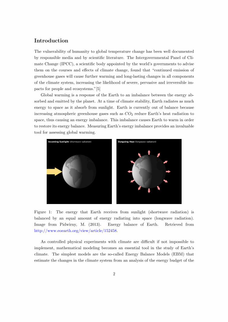
Global warming is a response of the Earth to an imbalance between the energy ab-

sorbed and emitted by the planet. At a time of climate stability, Earth radiates as much

energy to space as it absorb from sunlight. Earth is currently out of balance because

increasing atmospheric greenhouse gases such as CO2 reduce Earth’s heat radiation to

space, thus causing an energy imbalance. This imbalance causes Earth to warm in order

to restore its energy balance. Measuring Earth’s energy imbalance provides an invaluable

tool for assessing global warming.

Figure 1: The energy that Earth receives from sunlight (shortwave radiation) is

balanced by an equal amount of energy radiating into space (longwave radiation).

Image from Pidwirny, M. (2013). Energy balance of Earth. Retrieved from

http://www.eoearth.org/view/article/152458.

As controlled physical experiments with climate are difficult if not impossible to

implement, mathematical modeling becomes an essential tool in the study of Earth’s

climate. The simplest models are the so-called Energy Balance Models (EBM) that

estimate the changes in the climate system from an analysis of the energy budget of the

2

Earth.

This module introduces a Zonal Energy Balance Model (ZEBM) that describes the

evolution of the latitudinal distribution of Earth’s surface temperature. The model is

used to estimate the levels of Earth’s energy imbalance and corresponding zonal tem-

perature increase. Students working on the assignments in the last section will write a

computer code to obtain numerical solutions to ZEBM. They will play the role of an envi-

ronmental analyst by devising strategies for reduction of the growth rate of atmospheric

CO2 concentration in order to avoid “dangerous levels” of global warming.

The module has been written with the intention of providing a brief introduction

to the subject, directed mainly to instructors, to support the student’s assignments.

Instructors can use this content, together with the bibliographical references and other

resources provided, to organize the presentation of the topics to their students during

class time.

3

1 Derivation of the Model

We consider a Zonal Energy Balance Model that describes the evolution of the latitudinal

distribution of Earth’s surface temperature based on the assumption that the energy

received by the planet from Sun’s radiation must balance the radiation that the Earth is

loosing to space. The model takes into account that part of the incoming solar energy is

reflected back to space before entering the Earth, a phenomena know as albedo. It also

incorporates the warming effect of the accumulation of CO2 in the atmosphere.

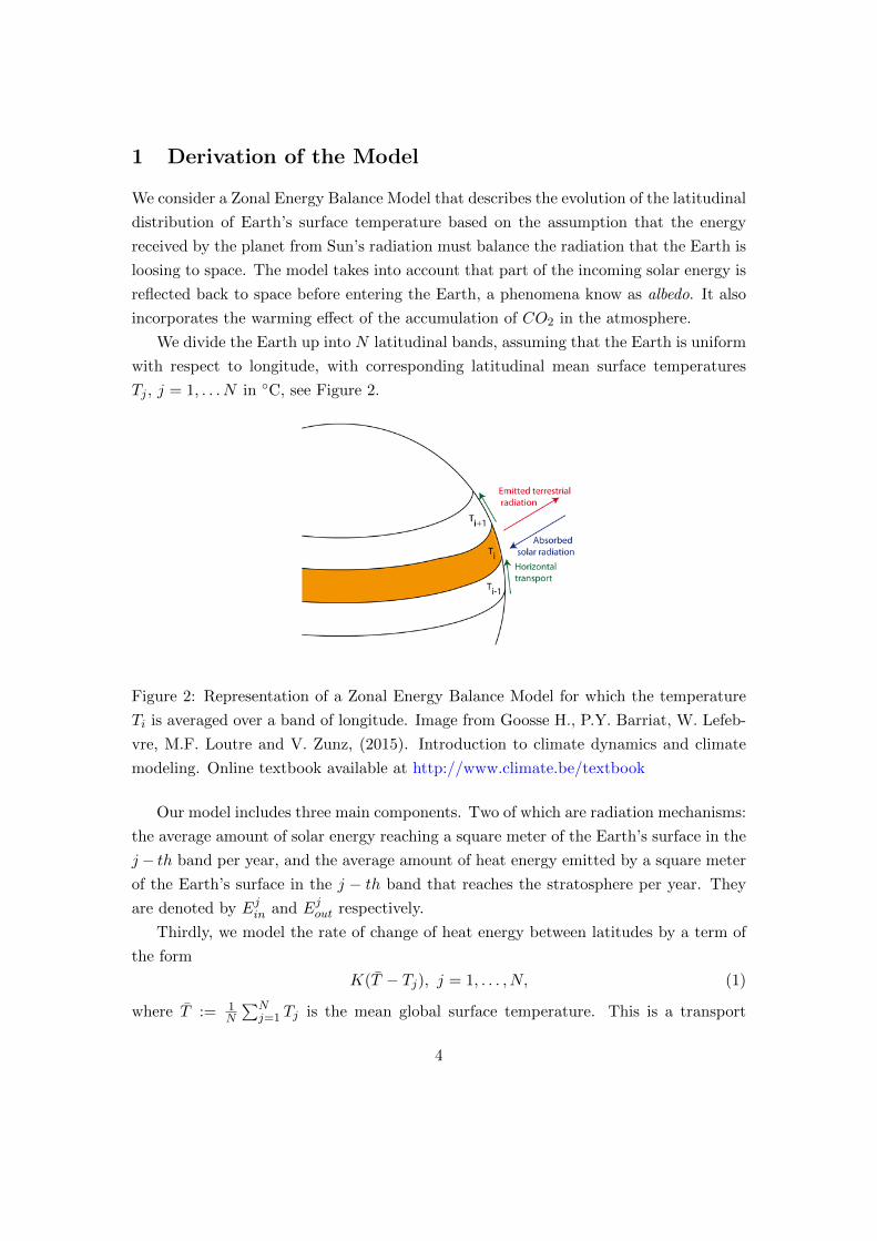
We divide the Earth up into N latitudinal bands, assuming that the Earth is uniform

with respect to longitude, with corresponding latitudinal mean surface temperatures

Tj , j = 1, . . . N in ◦C, see Figure 2.

Figure 2: Representation of a Zonal Energy Balance Model for which the temperature

Ti is averaged over a band of longitude. Image from Goosse H., P.Y. Barriat, W. Lefeb-

vre, M.F. Loutre and V. Zunz, (2015). Introduction to climate dynamics and climate

modeling. Online textbook available at http://www.climate.be/textbook

Our model includes three main components. Two of which are radiation mechanisms:

the average amount of solar energy reaching a square meter of the Earth’s surface in the

j− th band per year, and the average amount of heat energy emitted by a square meter

of the Earth’s surface in the j − th band that reaches the stratosphere per year. They

are denoted by Ejin and Ejout respectively.

Thirdly, we model the rate of change of heat energy between latitudes by a term of

the form

K(T − Tj), j = 1, . . . , N, (1)

where T := 1N

∑Nj=1 Tj is the mean global surface temperature. This is a transport

4

mechanism satisfying the requirement that the direction of heat transfer is from a region

of high temperature to another region of lower temperature. If the local temperature

at a particular latitud is greater than the global mean, heat will be taken out of that

latitude. Conversely, if the local temperature is colder than the global mean, that latitud

will gain heat. Notice the similarity of (1) with Newton’s law of cooling which states

that the rate of heat loss of a body is proportional to the difference in temperatures

between the body and its surroundings. The constant K = 1.6B is a positive empirical

constant (see [10, page 133]), where B = 1.9Wyr/m2 ◦C, obtained by linear regression

analysis of satellite data [3, Table 3], is the variation of the outgoing Earth’s radiation

per unit of change of global surface temperature.

Incoming Solar Radiation

The annual global mean incoming solar radiation or insolation is know as the solar

constant Q, with current value Q = 343Wyr/m2. Part of the incoming solar energy is

reflected back to to space before entering the Earth. This reflectivity is know as albedo

and is modeled by a factor α ∈ (0, 1).

In order to describe the variations of the albedo and insolation due to the latitude,

we represent the northern latitude by values y in the interval [0, 1] given by the function

y = sin(θ) with 0 ≤ θ ≤ π/2. Hence y = 0 corresponds to the equator, zero latitude,

and y = 1 corresponds to the pole, latitude θ = π.

Since the insolation Q is stronger at the equator than at the pole, an adjustment is

introduced as a function s(y) that represents the distribution of insolation over latitude.

Although s(y) is determined by astronomical calculations, it is uniformly approximated

by s(y) = 1− .482(3y2 − 1)/2 for 0 ≤ y ≤ 1 (see [7]). We will use the discrete version

sj = sN (j/N), j = 1, . . . , N,

where sN (y) = 1− .482(CNy2 − 1)/2 and CN = 6N2/(N + 1)(2N + 1).

The adjusted latitudinal insolation for the j − th band is given by

Qsj , j = 1, . . . , N. (2)

The constant CN is determined by assuming that 1N

∑Nj=1 sj = 1. This assumption

is required to obtain that the average of the latitudinal insolation (2) equals the global

mean insolation Q, that is 1N

∑Nj=1Qsj = Q.

Exercise 1. Use the identity∑N

j=1 j2 = N(N+1)(2N+1)

6 to verify that 1N

∑Nj=1 sj = 1.

5

The albedo is also dependent of the latitude. While the albedo for open water is

αw = 0.32, the albedo for snow-covered ice is αs = 0.62. We will assume that η = 0.95

is the location of the icecap, this correspond to 720 of latitude north, and consider that

the albedo αj is given by

αj =

αw, if j < n

αw+αs2 , if j = n

αs, ifj > n

,

where n = [0.95N ], and [x] is the largest integer not greater than x.

Putting these assumptions together we obtain that the incoming solar energy in the

j − th latitudinal band is given by

Ejin = (1− αj)Qsj , j = 1 . . . N. (3)

Outgoing Heat Radiation

With cumulative CO2 concentration and global mean surface temperature at the refer-

ence values c0 and T0 respectively, the outgoing Earth’s radiation is given by

Ejout = AN +BTj , j = 1, . . . , N. (4)

Since the outgoing–longwave–radiation (OLR) can be measured by satellites, and there

is a very good correlation between OLR and surface temperature, one can fit a straight

line to the measured data to obtain B. This procedure gives B = 1.9Wyr/m2 ◦C (see

[3, Table 3].) The constant AN , given in units of Wyr/m2, is obtained by assuming a

stable climate system, i.e.

Ejin − Ejout +K(T − Tj) = 0, j = 1, . . . , N, (5)

for T = T0.

Exercise 2. Show that

AN = (1− αN )Q−BT0, (6)

where αN = 1N

∑Nj=1 sjαj.

As the cumulative CO2 concentration c exceeds the reference value c0, the outgoing

Earth’s radiation is reduced by a term which, according to Arrhenius’ greenhouse law

6

[1], is proportional to the logarithm of the concentration of infrared-absorbing gasses in

the atmosphere1. We adopt the form

τB log2(c/c0). (7)

The parameter τ , given in units of ◦C, is the equilibrium climate sensitivity (ECS),

defined as the equilibrium change in annual mean global surface temperature following

a doubling of the atmospheric CO2 concentration. Notice that when c = 2c0 this term

is reduced to τB, which is the reduction of Earth’s radiation as a consequence of an

increase of the global surface temperature of τ ◦C due to doubling of atmospheric CO2

concentration. IPCC authors concluded that equilibrium climate sensitivity very likely

is greater than 1.5 ◦C and likely to lie in the range 2 to 4.5 ◦C , with a most likely value

of about 3 ◦C (see [8, 12]).

Putting together (4) and (7) we obtain the final expression for the outgoing Earth

radiation in the j − th latitudinal band:

Ejout = AN +BTj − τB log2(c/c0), j = 1, . . . , N. (8)

The Model

We now construct our model by stating that the rate of change of heat energy, given by

CdTjdt , j = 1, . . . , N , where C is the effective heat capacity, should be equal to that due

to the incoming solar radiation minus that due to the outgoing Earth’s radiation, plus

the heat gained or lost from transport. Thus,

CdTjdt

= (1− αj)Qsj − (AN +BTj) + τB log2(c/c0) +K(T − Tj), j = 1, . . . , N. (9)

This is a spatially discrete version of the well known Budyko-Sellers zonal energy balance

model (see [9]). Here Tj(t), j = 1, . . . , N is the latitudinal mean surface temperature at

time t ≥ 0. The constant C is the effective heat capacity, the energy need to raise the

global temperature by one degree Celsius. The heat capacity is commonly measured in

watt-years per square meter per deg Celsius (Wyr/m2 ◦C.) Its actual values depends on

the medium under consideration and vary from 0.55Wyr/m2 ◦C for soil/atmosphere to

1In 1896, Swedish scientist Svante Arrhenius was the first to calculate the warming power of excess

carbon dioxide (CO2). From his calculations, Arrhenius predicted that if human activities increased

CO2 levels in the atmosphere, a warming trend would result. In its original form, Arrhenius’ greenhouse

law reads as follows: “if the quantity of carbonic acid [CO2] increases in geometric progression, the

augmentation of the temperature will increase nearly in arithmetic progression.”

7

90Wyr/m2 ◦C for the ocean/atmosphere [6, page 15]. Since we are modeling the global

climate system we will assume that the heat capacity is constant over the entire globe

and equal to the weighted average C = 64Wyr/m2 ◦C obtained from the fact that the

surface of the Earth is approximately 71% water.

We will solve system (9) subject to the initial condition

Tj(0) =(1− αj)Qsj −AN + T0K

B +K, j = 1, . . . , N. (10)

Condition (10) is obtained by assuming a stable climate system, equation (5) with Ejinand Ejout given by (3) and (8) respectively, with T = T0 and c = c0.

Global Warming

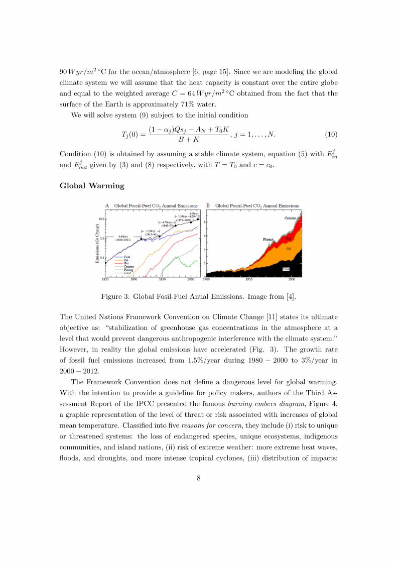
Figure 3: Global Fosil-Fuel Anual Emissions. Image from [4].

The United Nations Framework Convention on Climate Change [11] states its ultimate

objective as: “stabilization of greenhouse gas concentrations in the atmosphere at a

level that would prevent dangerous anthropogenic interference with the climate system.”

However, in reality the global emissions have accelerated (Fig. 3). The growth rate

of fossil fuel emissions increased from 1.5%/year during 1980 − 2000 to 3%/year in

2000− 2012.

The Framework Convention does not define a dangerous level for global warming.

With the intention to provide a guideline for policy makers, authors of the Third As-

sessment Report of the IPCC presented the famous burning embers diagram, Figure 4,

a graphic representation of the level of threat or risk associated with increases of global

mean temperature. Classified into five reasons for concern, they include (i) risk to unique

or threatened systems: the loss of endangered species, unique ecosystems, indigenous

communities, and island nations, (ii) risk of extreme weather: more extreme heat waves,

floods, and droughts, and more intense tropical cyclones, (iii) distribution of impacts:

8

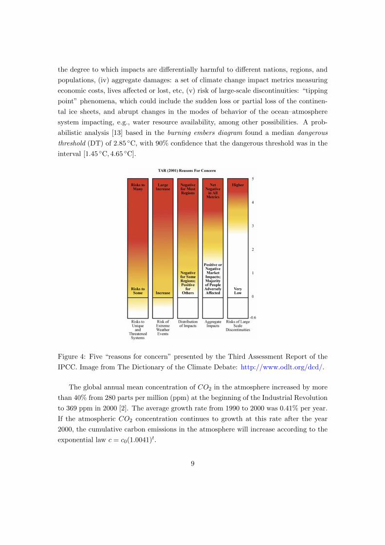
the degree to which impacts are differentially harmful to different nations, regions, and

populations, (iv) aggregate damages: a set of climate change impact metrics measuring

economic costs, lives affected or lost, etc, (v) risk of large-scale discontinuities: “tipping

point” phenomena, which could include the sudden loss or partial loss of the continen-

tal ice sheets, and abrupt changes in the modes of behavior of the ocean–atmosphere

system impacting, e.g., water resource availability, among other possibilities. A prob-

abilistic analysis [13] based in the burning embers diagram found a median dangerous

threshold (DT) of 2.85 ◦C, with 90% confidence that the dangerous threshold was in the

interval [1.45 ◦C, 4.65 ◦C].

Figure 4: Five “reasons for concern” presented by the Third Assessment Report of the

IPCC. Image from The Dictionary of the Climate Debate: http://www.odlt.org/dcd/.

The global annual mean concentration of CO2 in the atmosphere increased by more

than 40% from 280 parts per million (ppm) at the beginning of the Industrial Revolution

to 369 ppm in 2000 [2]. The average growth rate from 1990 to 2000 was 0.41% per year.

If the atmospheric CO2 concentration continues to growth at this rate after the year

2000, the cumulative carbon emissions in the atmosphere will increase according to the

exponential law c = c0(1.0041)t.

9

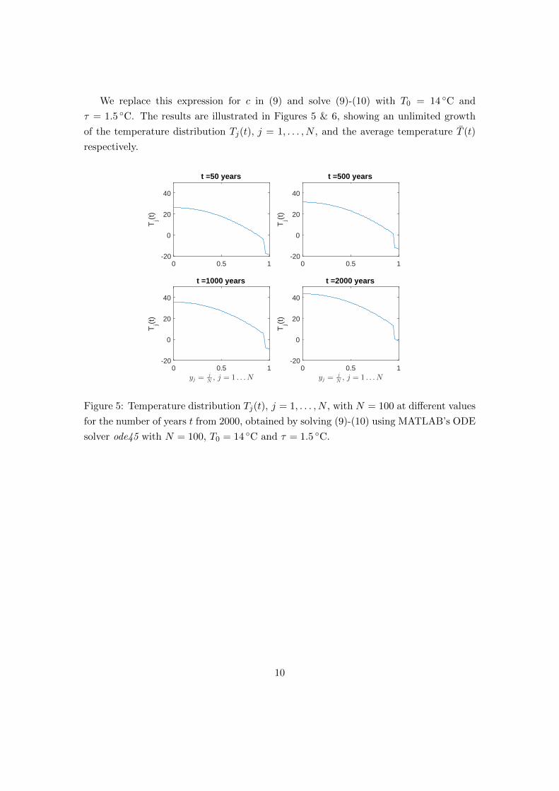
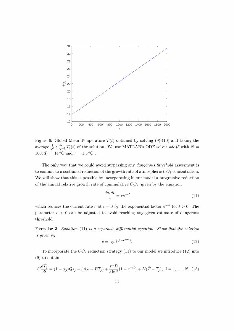
We replace this expression for c in (9) and solve (9)-(10) with T0 = 14 ◦C and

τ = 1.5 ◦C. The results are illustrated in Figures 5 & 6, showing an unlimited growth

of the temperature distribution Tj(t), j = 1, . . . , N , and the average temperature T (t)

respectively.

0 0.5 1-20

0

20

40

Tj(t

)

t =50 years

0 0.5 1-20

0

20

40

Tj(t

)

t =500 years

0 0.5 1yj =

j

N, j = 1 . . .N

-20

0

20

40

Tj(t

)

t =1000 years

0 0.5 1yj =

j

N, j = 1 . . .N

-20

0

20

40

Tj(t

)t =2000 years

Figure 5: Temperature distribution Tj(t), j = 1, . . . , N , with N = 100 at different values

for the number of years t from 2000, obtained by solving (9)-(10) using MATLAB’s ODE

solver ode45 with N = 100, T0 = 14 ◦C and τ = 1.5 ◦C.

10

0 200 400 600 800 1000 1200 1400 1600 1800 2000

t

12

14

16

18

20

22

24

26

28

30

32

T(t)

Figure 6: Global Mean Temperature T (t) obtained by solving (9)-(10) and taking the

average 1N

∑Nj=1 Tj(t) of the solution. We use MATLAB’s ODE solver ode45 with N =

100, T0 = 14 ◦C and τ = 1.5 ◦C .

The only way that we could avoid surpassing any dangerous threshold assessment is

to commit to a sustained reduction of the growth rate of atmospheric CO2 concentration.

We will show that this is possible by incorporating in our model a progressive reduction

of the annual relative growth rate of commulative CO2, given by the equation

dc/dt

c= re−εt (11)

which reduces the current rate r at t = 0 by the exponential factor e−εt for t > 0. The

parameter ε > 0 can be adjusted to avoid reaching any given estimate of dangerous

threshold.

Exercise 3. Equation (11) is a separable differential equation. Show that the solution

is given by

c = c0erε(1−e−εt). (12)

To incorporate the CO2 reduction strategy (11) to our model we introduce (12) into

(9) to obtain

CdTjdt

= (1− αj)Qsj − (AN +BTj) +rτB

ε ln 2(1− e−εt) +K(T − Tj), j = 1, . . . , N. (13)

11

This is a linear system of non-autonomous (time-dependent forcing term) differential

equations of the form

dTjdt

+ βTj = γj + δ(1− e−εt) + λ(T − Tj), j = 1, . . . , N, (14)

with β = B/C, γj = ((1− αi)Qsj −AN )/C, δ = rτBεC ln 2 , and λ = K/C.

The following convergence theorem shows that it is possible to choose ε > 0 such

that global mean temperatures would remain below dangerous levels of global warming.

The proof is left as an assignment for the interested reader.

Theorem 1. Let Tj(t), j = 1, . . . , N , be a solution of (14)-(10). Then

limt→∞

Tj(t) = T ∗j , (15)

where

T ∗j =γj + δ + λT ∗

β + λ, (16)

with,

T ∗ =γ + δ

β

γ =Q(1− αN )−AN

C

αN =1

N

N∑j=1

sjαj .

Moreover, T (t) < T ∗ for t ≥ 0.

Exercise 4. Show that

T ∗ = T0 +rτ

ε ln 2(17)

Theorem 1 and equation (17) shows that by choosing ε > 0 such that

rτ

ε ln 2= DT, (18)

for a given dangerous threshold DT , the global temperature average T will remain below

DT avoiding dangerous levels of global warming.

As an example lets assume we are in the year 2000 with reference values for the global

mean surface temperature T0 = 14 ◦C and cumulative carbon emissions c0 = 369 ppm.

We consider the conservative scenario of an equilibrium climate sensitivity τ = 1.5 ◦C,

dangerous threshold DT = 2.85 ◦C, and initial growth rate r = 0.41% yearly.

12

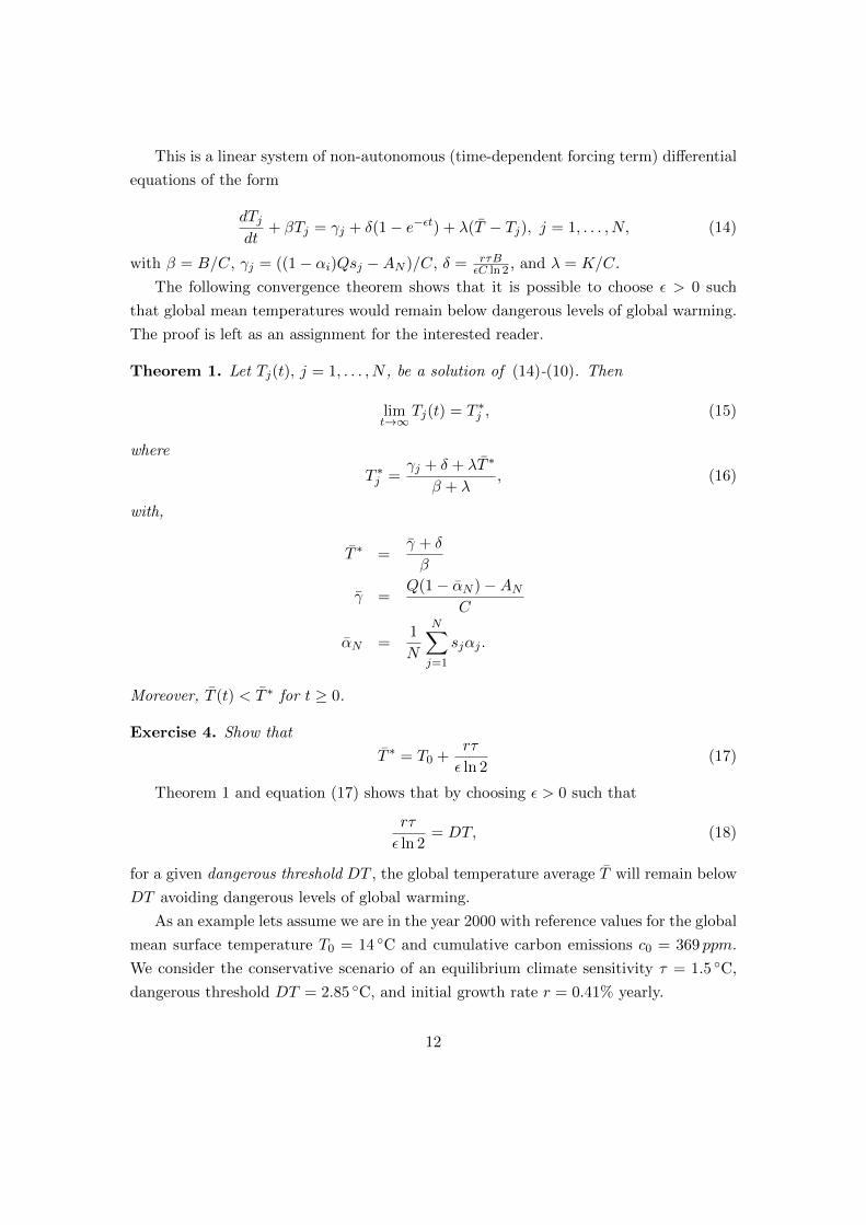
Solving (14)-(10) with N = 100 and ε = rτ/DT ln 2 ≈ 0.0031 satisfying (18), we

obtain Figure 7 describing the temperature distribution Tj(t), j = 1 . . . N , at different

values for the number of years t from 2000.

0 0.5 1-20

0

20

40

Tj(t

)

t =10 years

0 0.5 1-20

0

20

40

Tj(t

)

t =100 years

0 0.5 1yj =

jN, j = 1 . . . N

-20

0

20

40

Tj(t

)

t =200 years

0 0.5 1yj =

jN, j = 1 . . . N

-20

0

20

40T

j(t)

t =400 years

Figure 7: Temperature distribution Tj(t), j = 1, . . . , N , with N = 100 at different values

for number of years t from 2000, obtained by solving (14) with MATLAB’s ODE solver

ode45. We use the values τ = 1.5 ◦C, DT = 2.85◦C, r = 0.41%, and ε = rτ/DT ln 2 ≈0.0031 satisfying (18). The dashed line corresponds to T ∗j as given by (16).

Notice that Figure 7 suggests that Tj(t) < T ∗j , j = 1, . . . , N , for t ≥ 0, where T ∗j is

represented with a dashed line. This is not predicted by Theorem 1 which does predict

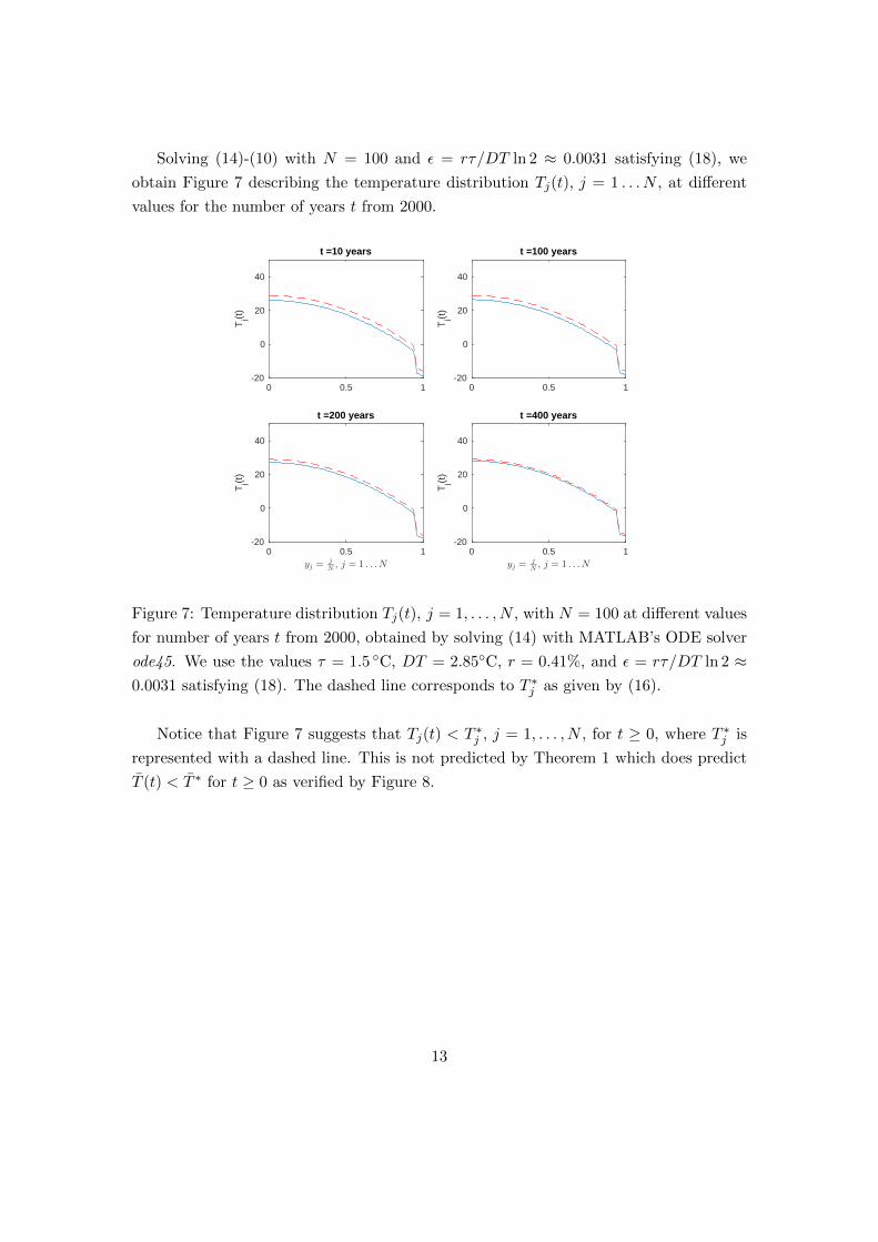
T (t) < T ∗ for t ≥ 0 as verified by Figure 8.

13

0 200 400 600 800 1000 1200 1400

t

13.5

14

14.5

15

15.5

16

16.5

17

T(t)

Figure 8: Global Mean Temperature T (t) obtained by solving (14) and taking the average1N

∑Nj=1 Tj(t) of the solution. The dashed line corresponds to the value of T ∗. We use

MATLAB’s ODE solver ode45 with N = 100, τ = 1.5 ◦C, DT = 2.85◦C, r = 0.41%, and

ε = rτ/DT ln 2 ≈ 0.0031 satisfying (18).

14

2 Assignments

Assignment 1. Write a computer code to solve system (14)-(10) numerically. We

recommend the MATLAB solver ode45, or the Mathematica function NDSolve, to

obtain an accurate solution.

Assignment 2. Assume for simplicity that you are in the year 2000 with reference values

for the global mean surface temperature T0 = 14 ◦C, cumulative carbon concentration

c0 = 369 ppm, and initial growth rate of fossil fuel r = 0.41%. Adopt your favorite

values for the equilibrium climate sensitivity τ and dangerous threshold DT . With a

choice of ε > 0 satisfying (18), use the script developed in Assignment 1 to verify that

the global temperature average T (t) will remain below T0 + DT for t > 0.Describe your

results with graphical outputs similar to Figures 7 & 8.

15

References

[1] Arrhenius, Svante http://en.wikipedia.org/wiki/Svante Arrhenius

[2] Dlugokencky, E (5 February 2016), “Annual Mean Carbon Dioxide Data”. Earth

System Research Laboratory. National Oceanic & Atmospheric Administration.

https://en.wikipedia.org/wiki/Carbon dioxide in Earth%27s atmosphere#cite note-

NOAA CO2annual-5.

[3] C. Graves, W-H. Lee, and G. North, New parameterizations and sensitivities for

simple climate models, i. Geophys. Res. 198 (D3) (1993) 50255036.

[4] Hansen i, Kharecha P, Sato M, Masson-Delmotte V, et al. Assessing “Dan-

gerous Climate Change”: Required Reduction of Carbon Emissions to Protect

Young People, Future Generations and Nature, PLoS ONE 8(12) (2013): e81648.

doi:10.1371/journal.pone.0081648

[5] IPCC Climate Change 2014 Synthesis Report: http://www.ipcc.ch/report/ar5/syr/

[6] H. Kaper & H. Engler, Mathematics & Climate, SIAM (2013).

[7] G.R. North, Theory of energy-balance climate models, i. Atmos. Sci. 32 (11) (1975)

20332043.

[8] D. Nuccitelli, What you need to know about climate sensitivity, Climate Consensus

- the 97%, theguardian.com, http://gu.com/p/3fehq/sbl

[9] C. Rackauckas & J. Walsh, On the Budyko-Sellers energy balance climate model with

ice line coupling, Discrete and Continuous Dynamical Systems, Series B, Volume

20, Number 7 (2015) 21872216.

[10] K. K. Tung, Topics in Mathematical Modeling, Princeton University Press, Prince-

ton, New Jersey, USA, 2007.

[11] United Nations Framework Convention on Climate Change (1992) Available:

http://www.unfccc.int.

[12] Wikipedia, Climate Sensitivity: http://en.wikipedia.org/wiki/Climate sensitivity

[13] Schneider SH, Mastrandrea MD, Probabilistic assessment “dangerous” climate

change and emissions pathways, Proc Natl Acad Sci USA 102 (2005) 15728 –15735,

doi: 10.1073/pnas.0506356102.

16