global testing and testing for high-dimensional …tcai/paper/testing...1.1.global testing for...

Global Testing andLarge-Scale MultipleTesting forHigh-DimensionalCovariance Structures

T. Tony Cai1

1Department of Statistics, The Wharton School, University of Pennsylvania,

Philadelphia, USA, 19104; email: [email protected]

Xxxx. Xxx. Xxx. Xxx. YYYY. AA:1–27

This article’s doi:

10.1146/((please add article doi))

Copyright c© YYYY by Annual Reviews.

All rights reserved

Keywords

Correlation matrix, covariance matrix, differential network, false

discovery proportion, false discovery rate, Gaussian graphical model,

global testing, multiple testing, null distribution, precision matrix,

thresholding.

Abstract

Driven by a wide range of contemporary applications, statistical infer-

ence for covariance structures has been an active area of current research

in high-dimensional statistics. This paper provides a selective survey

of some recent developments in hypothesis testing for high-dimensional

covariance structures, including global testing for the overall pattern of

the covariance structures and simultaneous testing of a large collection

of hypotheses on the local covariance structures with false discovery

proportion (FDP) and false discovery rate (FDR) control. Both one-

sample and two-sample settings are considered. The specific testing

problems discussed include global testing for the covariance, correla-

tion, and precision matrices, and multiple testing for the correlations,

Gaussian graphical models, and differential networks.

1

Contents

1. Introduction . . . . . . . . . . . . . . . . . . . . . . . . . . . . . . . . . . . . . . . . . . . . . . . . . . . . . . . . . . . . . . . . . . . . . . . . . . . . . . . . . . . . . . . . . . . . . . . . . . 31.1. Global Testing for High-Dimensional Covariance Structures . . . . . . . . . . . . . . . . . . . . . . . . . . . . . . . . . . . . . . . . . . . 41.2. Multiple Testing for Local Covariance Structures . . . . . . . . . . . . . . . . . . . . . . . . . . . . . . . . . . . . . . . . . . . . . . . . . . . . . . 61.3. Notation and Definitions . . . . . . . . . . . . . . . . . . . . . . . . . . . . . . . . . . . . . . . . . . . . . . . . . . . . . . . . . . . . . . . . . . . . . . . . . . . . . . . . 7

2. Global Testing for Covariance Structures . . . . . . . . . . . . . . . . . . . . . . . . . . . . . . . . . . . . . . . . . . . . . . . . . . . . . . . . . . . . . . . . . . . . 82.1. Testing a Simple Global Null Hypothesis H0 : Σ = I . . . . . . . . . . . . . . . . . . . . . . . . . . . . . . . . . . . . . . . . . . . . . . . . . . 82.2. Testing a Composite Global Null Hypothesis in the One-Sample Case . . . . . . . . . . . . . . . . . . . . . . . . . . . . . . . . 92.3. Testing for Equality of Two Covariance Matrices H0 : Σ1 = Σ2 . . . . . . . . . . . . . . . . . . . . . . . . . . . . . . . . . . . . . . 92.4. Global Testing for Differential Correlations H0 : R1 −R2 = 0 . . . . . . . . . . . . . . . . . . . . . . . . . . . . . . . . . . . . . . . . 112.5. Global Testing for Differential Network H0 : Ω1 −Ω2 = 0 . . . . . . . . . . . . . . . . . . . . . . . . . . . . . . . . . . . . . . . . . . . . 12

3. Large-Scale Multiple Testing for Local Covariance Structures . . . . . . . . . . . . . . . . . . . . . . . . . . . . . . . . . . . . . . . . . . . . . . 143.1. The Main Ideas and Common Features . . . . . . . . . . . . . . . . . . . . . . . . . . . . . . . . . . . . . . . . . . . . . . . . . . . . . . . . . . . . . . . . 143.2. Multiple Testing for Correlations . . . . . . . . . . . . . . . . . . . . . . . . . . . . . . . . . . . . . . . . . . . . . . . . . . . . . . . . . . . . . . . . . . . . . . . 163.3. Multiple Testing for A Gaussian Graphical Model . . . . . . . . . . . . . . . . . . . . . . . . . . . . . . . . . . . . . . . . . . . . . . . . . . . . . . 193.4. Multiple Testing for Differential Networks. . . . . . . . . . . . . . . . . . . . . . . . . . . . . . . . . . . . . . . . . . . . . . . . . . . . . . . . . . . . . . 20

4. Discussion and Future Issues . . . . . . . . . . . . . . . . . . . . . . . . . . . . . . . . . . . . . . . . . . . . . . . . . . . . . . . . . . . . . . . . . . . . . . . . . . . . . . . . . 21

2 Tony Cai

1. Introduction

Analysis of high dimensional data, whose dimension p can be much larger than the sample

size n, has emerged as one of the most important and active areas of current research in

statistics. It has a wide range of applications in many fields, including genomics, medical

imaging, signal processing, social science, and financial economics. Covariance structure

plays a central role in many of these analyses. In addition to being of significant interest

in its own right for many important applications, knowledge of the covariance structures

is critical for a large collection of fundamental statistical methods, including the principal

component analysis, discriminant analysis, clustering analysis, and regression analysis.

There have been significant recent advances on statistical inference for high-dimensional

covariance structures. These include estimation of and testing for large covariance matrices,

volatility matrices, correlation matrices, precision matrices, Gaussian graphical models,

differential correlations, and differential networks. The difficulties of these high-dimensional

statistical problems can be traced back to the fact that the usual sample covariance matrix,

which performs well in the classical low-dimensional cases, fails to produce good results in

the high-dimensional settings. For example, when p > n, the sample covariance matrix is

not invertible, and consequently does not lead directly to an estimate of the precision matrix

(the inverse of the covariance matrix) which is required in many applications. It is also well

known that the empirical principal components of the sample covariance matrix can be

nearly orthogonal to the corresponding principal components of the population covariance

matrix in the high-dimensional settings. See, e.g., Johnstone (2001), Paul (2007), and

Johnstone and Lu (2009).

Structural assumptions are needed for accurate estimation of high-dimensional covari-

ance and precision matrices. A collection of smoothing and regularization methods have

been developed for estimation of covariance, correlation, and precision matrices under the

various structural assumptions. These include the banding methods in Wu and Pourahmadi

(2009) and Bickel and Levina (2008a), tapering in Furrer and Bengtsson (2007) and Cai

et al. (2010), thresholding rules in Bickel and Levina (2008b), El Karoui (2008), Rothman

et al. (2009), Cai and Liu (2011), and Fan et al. (2011), penalized log-likelihood estimation

in Huang et al. (2006), Yuan and Lin (2007), d’Aspremont et al. (2008), Banerjee et al.

(2008), Rothman et al. (2008), Lam and Fan (2009), Ravikumar et al. (2011), and Chan-

drasekaran et al. (2012), regularizing principal components in Johnstone and Lu (2009),

Zou et al. (2006), Cai et al. (2013, 2015), Fan et al. (2013), and Vu and Lei (2013), and

penalized regression for precision matrix estimation, Gaussian graphical models, and differ-

ential networks in Meinshausen and Buhlmann (2006), Yuan (2010), Cai et al. (2011), Sun

and Zhang (2013), Zhao et al. (2014), and Ren et al. (2015).

Optimal rates of convergence and adaptive estimation for high-dimensional covariance

and precision matrices have been studied. See, for example, Cai et al. (2010); Cai and

Yuan (2012) for bandable covariance matrices, Cai and Zhou (2012); Cai and Liu (2011)

for sparse covariance matrices, Cai, Ren, and Zhou (2013) for Toeplitz covariance matrices,

Cai et al. (2015) for sparse spiked covariance matrices, and Cai et al. (2016) for sparse

precision matrices. It should be noted that many of these matrix estimation problems

exhibit new features that are significantly different from those that occur in the conventional

nonparametric function estimation problems and require the development of new technical

tools which can be useful for other estimation and inference problems as well. See Cai

et al. (2016) for a survey of the recent results on optimal and adaptive estimation, and for

a discussion of some key technical tools used in the theoretical analyses.

www.annualreviews.org • Hypothesis Testing for Covariance Structures 3

Parallel to estimation, there have been significant recent developments on the methods

and theory for hypothesis testing on high-dimensional covariance structures. There are a

wide array of applications, including brain connectivity analysis (Shaw et al. 2006), gene

co-expression network analysis (Carter et al. 2004; Lee et al. 2004; Zhang et al. 2008; Dubois

et al. 2010; Fuller et al. 2007), differential gene expression analysis (Shedden and Taylor

(2005); de la Fuente (2010); Ideker and Krogan (2012); Fukushima (2013)), and correlation

analysis of factors that interact to shape children’s language development and reading ability

(Dubois et al. 2010; Hirai et al. 2007; Raizada et al. 2008; Zhu et al. 2005).

High dimensionality and dependency impose significant methodological and technical

challenges. This is particularly true for testing on the structure of precision matrices and

differential networks as there is no “sample precision matrix” as the natural starting point.

The problems of hypothesis testing for high-dimensional covariance structures can be di-

vided into two types: global testing for the overall pattern of the covariance structures and

simultaneous testing of a large collection of hypotheses for the local covariance structures

such as pairwise correlations or changes on conditional dependence. These two types of

testing problems are related but also very different in nature. We discuss them separately

in the present paper.

In the classical setting of low-dimension and large sample size, several methods have

been developed for testing specific global patterns of covariance matrices. In the high-

dimensional settings, these methods either do not perform well or are no longer applicable.

A collection of new global testing procedures have been developed in the last few years

both in the one-sample and two-sample cases. In addition to global testing, large-scale

multiple testing for high-dimensional covariance structures, where one tests simultaneously

thousands or millions of hypotheses on the local covariance structures or the changes of the

local covariance structures, is an important and challenging problem. For a range of applica-

tions, a common feature in the covariance structures is sparsity under the alternatives. We

will discuss a few recently proposed methods for both global testing and large-scale multiple

testing for high-dimensional covariance structures that leverage the sparsity information.

We will conclude with a discussion on some future issues and open problems.

Throughout the paper, Σ = (σi,j), R = (ri,j), Ω = (ωi,j), and I denote the covariance,

correlation, precision, and identity matrices, respectively. in the one-sample case, we assume

that we observe a random sample X1, . . . ,Xn which consists of n independent copies of

a p-dimensional random vector X = (X1, . . . , Xp)ᵀ following some distribution with mean

µ = (µ1, ..., µp) and covariance matrix Σ = (σi,j)p×p. The sample mean is X = 1n

∑nk=1 Xk

and sample covariance matrix Σ = (σi,j)p×p is defined as

Σ =1

n

n∑k=1

(Xk − X)(Xk − X)ᵀ. (1)

In the two-sample case, we observe two independent random samples, X1, . . . ,Xn1 are

i.i.d. from a p-variate distribution with µ1 = (µ1,1, ..., µp,1)ᵀ and covariance matrix Σ1 =

(σi,j,1)p×p and Y1, . . . ,Yn2 are i.i.d. from a distribution with µ2 = (µ1,2, ..., µp,2)ᵀ and

covariance matrix Σ2 = (σi,j,2)p×p. Given the two independent random samples, define

the sample means by X = 1n1

∑n1k=1 Xk and Y = 1

n2

∑n2k=1 Yk and the sample covariance

matrices Σ1 = (σi,j,1)p×p and Σ2 = (σi,j,2)p×p by

Σ1 =1

n1

n1∑k=1

(Xk − X)(Xk − X)ᵀ and Σ2 =1

n2

n2∑k=1

(Yk − Y)(Yk − Y)ᵀ. (2)

4 Tony Cai

1.1. Global Testing for High-Dimensional Covariance Structures

Global testing has been relatively well studied in the one-sample case. Several interesting

two-sample global testing problems have also been investigated recently. We give a brief

discussion here and consider these problems in detail in Section 2.

1.1.0.1. Testing the Simple Global Null Hypothesis H0 : Σ = I. Testing a simple

global null hypothesis H0 : Σ = I occupies a special position in the methods and theory for

testing high-dimensional covariance structures. Much of the random matrix theory has been

developed in the null case Σ = I and testing for H0 : Σ = I is often used as an immediate

application for the results from the random matrix theory. A collection of testing methods

has been proposed in the literature, including tests based on the spectral norm (largest

eigenvalue), tests based on the Frobenius norm, and tests using the maximum entrywise

deviation. A concise summary of the methods for testing the global null H0 : Σ = I is given

in Section 2.1.

1.1.0.2. Testing a Composite Global Null Hypothesis in the One-Sample Case.

In addition to testing the simple null H0 : Σ = I, it is also of interest to test a range

of composite global null hypotheses, including testing for sphericity with H0 : Σ = σ2I,

testing for H0 : Σ is diagonal, which is equivalent to H0 : R = I, and testing for short-

range dependence H0 : ri,j = 0 for all |i− j| ≥ k. For testing against a composite null, the

standard random theory results are often not directly applicable. Methods for testing these

one-sample composite global nulls will be discussed in Section 2.2.

1.1.0.3. Testing for Equality of Two Covariance Matrices H0 : Σ1 = Σ2. Test-

ing the equality of two covariance matrices Σ1 and Σ2 is an important problem. Many

statistical procedures including the classical Fisher’s linear discriminant analysis rely on

the fundamental assumption of equal covariance matrices. The likelihood ratio test (LRT)

is commonly used in the conventional low-dimensional case and enjoys certain optimality

properties. In the high-dimensional setting where p > n, the LRT is not applicable. There

are two types of tests in this setting: one is based on the maximum entrywise deviation and

another is based on the Frobenius norm of Σ1 − Σ2. The former is particularly powerful

when Σ1−Σ2 is “sparse” under the alternative and the latter performs well when Σ1−Σ2 is

“dense”. Section 2.3 discusses a recent proposal in Cai et al. (2013) that is powerful against

sparse alternatives and robust with respect to the population distributions. A summary of

a few Frobenius norm based methods is also given.

1.1.0.4. Global Testing for Differential Correlations H0 : R1 −R2 = 0. Differential

gene expression analysis is widely used in genomics for identifying disease-associated genes

for complex diseases (Shedden and Taylor (2005); Bandyopadhyay et al. (2010); de la Fuente

(2010); Ideker and Krogan (2012); Fukushima (2013)). For example, de la Fuente (2010)

demonstrated that the gene expression networks can vary in different disease states and the

differential correlations in gene expression are useful in disease studies. Global testing for

the differential correlations H0 : R1−R2 = 0 based on two independent random samples is

complicated as the entries of the sample differential correlation matrix are correlated under

the null H0. Section 2.4 considers a test recently introduced in Cai and Zhang (2016) that

is based on the maximum entrywise deviation. The test is powerful when the differential

correlation matrix is sparse under the alternative.


1.1.0.5. Global Testing for Differential Network H0 : Ω1−Ω2 = 0. Gaussian graphical

models provide a powerful tool for modeling the conditional dependence relationships among

a large number of random variables in a complex system. Applications include portfolio

optimization, speech recognition, and genomics. It is well known that the structure of an

undirected Gaussian graph is characterized by the precision matrix of the corresponding

distribution (Lauritzen 1996). In addition to inference for a given Gaussian graph, it is

of significant interest in many applications to understand whether and how the network

changes between disease states (de la Fuente 2010; Ideker and Krogan 2012; Hudson et al.

2009; Li et al. 2007; Danaher et al. 2014; Zhao et al. 2014; Xia et al. 2015).

The problem of detecting whether the network changes between disease states under

the Gaussian graphical model framework can be formulated as testing

H0 : ∆ = 0 versus H1 : ∆ 6= 0

where ∆ = (δi,j) = Ω1 − Ω2 is called the differential network. Equality of two precision

matrices is mathematically equivalent to equality of two covariance matrices. However, it

is often the case in many applications Ω1 and Ω2 are sparse and it is important to test the

precision matrices directly in order to incorporate the sparsity information in the testing

procedure. Section 2.5 discusses a testing method recently proposed in Xia et al. (2015)

that is based on a penalized regression approach.

1.2. Multiple Testing for Local Covariance Structures

Simultaneously testing a large number of hypotheses on local covariance structures arises in

many important applications including genome-wide association studies (GWAS), phenome-

wide association studies (PheWAS), and brain imaging. A common goal in multiple testing

is often to control the false discovery proportion (FDP), which is defined to be the proportion

of false positives among all rejections, and its expectation, the false discovery rate (FDR).

Simultaneous testing for the covariance structures with FDP and FDR control is technically

challenging, both in constructing a suitable test statistic for testing a given hypothesis and

establishing its null distribution and in developing a multiple testing procedure to account

for the multiplicity and dependency so that the overall FDP and FDR are controlled.

Multiple testing has been well studied in the literature, especially in the case where the

test statistics are independent. See, for example, Benjamini and Hochberg (1995); Storey

(2002); Efron (2004); Genovese and Wasserman (2004); Sun and Cai (2007). Standard

FDR control procedures, such as the Benjamini-Hochberg (B-H) procedure (Benjamini and

Hochberg 1995), typically built under the independence assumption, would fail to provide

desired error controls in the presence of strong correlation, particularly when the signals

are sparse. The effects of dependency on multiple testing procedures have been considered,

for example, in Benjamini and Yekutieli (2001); Storey et al. (2004); Qiu et al. (2005);

Farcomeni (2007); Wu (2008); Efron (2007); Sun and Cai (2009); Sun et al. (2015). In

particular, Qiu et al. (2005) demonstrated that the dependency effects can significantly

deteriorate the performance of many multiple testing procedures. Farcomeni (2007) and

Wu (2008) showed that the FDR is controlled at the nominal level by the B-H procedure

under some stringent dependency assumptions. The procedure in Benjamini and Yekutieli

(2001) allows the general dependency by paying a logarithmic term loss on the FDR which

makes the method very conservative.

A natural starting point for large-scale multiple testing for local covariance structures

6 Tony Cai

is the sample covariance or correlation matrix, whose entries are intrinsically heteroscedas-

tic and dependent even if the original observations are independent. The sample covari-

ances/correlations may have a wide range of variability and their dependence structure is

rather complicated. The analysis of these large-scale multiple testing problems poses many

statistical challenges not present in smaller scale studies.

1.2.0.1. Multiple Testing for Correlations. The problem of correlation detection arises

in both one-sample and two-sample settings. In the one-sample case, one wishes to simul-

taneously test (p2 − p)/2 hypotheses

H0,i,j : ri,j = 0 versus H1,i,j : ri,j 6= 0, for 1 ≤ i < j ≤ p.

In the two-sample case, one is interested in the simultaneous testing of correlation changes,

H0,i,j : ri,j,1 = ri,j,2 versus H1,i,j : ri,j,1 6= ri,j,2, for 1 ≤ i < j ≤ p.

Section 3.2 discusses multiple testing procedures for correlations recently introduced in Cai

and Liu (2015) in both the one-sample and two-sample settings.

1.2.0.2. Multiple Testing for Gaussian Graphical Models. As mentioned earlier,

Gaussian graphical models have a wide range of applications and the conditional dependence

structure is completely characterized by the corresponding precision matrix Ω = (ωi,j)p×pof the distributions. Given an i.i.d. random sample, the problem of multiple testing for

a Gaussian graphical model can thus be formulated as simultaneously testing (p2 − p)/2hypotheses on the off-diagonal entries of the precision matrix Ω,

H0,i,j : ωi,j = 0 versus H1,i,j : ωi,j 6= 0, 1 ≤ i < j ≤ p.

Section 3.3 discusses a multiple testing procedure for Gaussian graphical models proposed

in Liu (2013), which was shown to control both the FDP and FDR asymptotically.

1.2.0.3. Multiple Testing for Differential Networks. Differential network analysis has

many important applications in genomics and other fields. If the global null hypothesis

H0 : ∆ ≡ Ω1 −Ω2 = 0 is rejected, it is often of significant interest to investigate the local

structures of the differential network ∆. A natural approach is to carry out simultaneous

testing for the (p2 − p)/2 hypotheses on the off-diagonal entries of ∆ = (δi,j),

H0,i,j : δi,j = 0 versus H1,i,j : δi,j 6= 0, 1 ≤ i < j ≤ p. (3)

This problem was recently studied in Xia et al. (2015). A procedure for simultaneously

testing the hypotheses in (3) was developed and shown to control the FDP and FDR

asymptotically. Section 3.4 will discuss this procedure in detail.

1.3. Notation and Definitions

We introduce here notation and definitions that will be used in the rest of the paper. Vectors

and matrices are denoted by boldfaced letters.

For a vector a = (a1, . . . , ap)ᵀ ∈ Rp, define the `q norm by ‖a‖q = (

∑pi=1 |ai|

q)1/q for

1 ≤ q ≤ ∞. A vector a ∈ Rp is called k-sparse if it has at most k nonzero entries. We say


a matrix A is k-sparse if each row/column has at most k nonzero entries. For any vector

a ∈ Rp, let a−i denote the vector in Rp−1 by removing the ith entry from a. For a matrix

A ∈ Rp×q, Ai,−j denotes the ith row of A with its jth entry removed and A−i,j denotes the

jth column of A with its ith entry removed. The matrix A−i,−j denotes a (p− 1)× (q− 1)

matrix obtained by removing the ith row and jth column of A. For 1 ≤ w ≤ ∞ and a matrix

A = (ai,j)p×p, the matrix `w norm of a matrix A is defined as ‖A‖w = max‖x‖w=1 ‖Ax‖w.

The spectral norm is the `2 norm. The Frobenius norm of A is ‖A‖F =√∑

i,j a2i,j , and

the trace of A is tr(A) =∑i ai,i.

For a set H, denote by |H| the cardinality of H. For two sequences of positive real

numbers an and bn, write an = O(bn) if there exists a constant C such that |an| ≤ C|bn|holds for all n, write an = o(bn) if limn→∞ an/bn = 0, an . bn means an ≤ Cbn for all

n, and an bn if an . bn and bn . an. We use I· to denote the indicator function,

use φ and Φ to denote respectively the density and cumulative distribution function of

the standard normal distribution, and use G(t) = 2 − 2Φ(t) for the tail probability of the

standard normal distribution.

2. Global Testing for Covariance Structures

We discuss in this section several problems on global testing for the overall patterns of the

covariance structures. As mentioned in the introduction, in many applications, a common

feature in the covariance structures is sparsity under the alternatives. A natural strategy

to leverage the sparsity information is to use the maximum of entrywise deviations from

the null as the test statistic. The null distribution of such a statistic is often the type I

extreme value distribution. In this paper, we say a test statistic Mn,p has asymptotically

the extreme value distribution of type I if for any given t ∈ R,

P (Mn,p − 4 log p+ log log p ≤ t)→ exp

(− 1√

8πe−t/2

), as n, p→∞. (4)

The 1− α quantile, denoted by qα, of the type I extreme value distribution is given by

qα = − log(8π)− 2 log log(1− α)−1. (5)

We begin with a brief summary of the methods for testing for a simple null H0 : Σ = I.

This problem has been well studied in the literature due to its close connection to the

random matrix theory.

2.1. Testing a Simple Global Null Hypothesis H0 : Σ = I

In the classical setting where the dimension p is fixed and the distribution is Gaussian, the

most commonly used test for testing the simple null H0 : Σ = I is the likelihood ratio

test, whose test statistic is given by LR = tr(Σ) − log det(Σ) − p. It is known that the

asymptotic null distribution of the test statistic LR is χ2p(p+1)/2. See Anderson (2003);

Muirhead (1982). When the dimension p grows with the sample size n, the standard LRT

is no longer applicable. Bai et al. (2009) proposed a corrected LRT for which the test

statistic has a Gaussian limiting null distribution when p/n → c ∈ (0, 1). The result is

further extended in Jiang et al. (2012); Zheng et al. (2015).

In the high-dimensional setting, a natural approach to testing the simple null H0 : Σ = I

is to use test statistics that are based on some distance ‖Σ − I‖ where ‖ · ‖ is a matrix

8 Tony Cai

norm such as the spectral norm or the Frobenius norm. When the dimension p and the

sample size n are comparable, i.e., p/n→ γ ∈ (0,∞), testing of the hypotheses H0 : Σ = I

against H1 : Σ 6= I has been considered by Johnstone (2001) in the Gaussian case, Soshnikov

(2002) in the sub-Gaussian case, and by Peche (2009) in a more general setting with moment

conditions and where the ratio p/n can converge to either a positive number γ, 0 or ∞.

Johnstone (2001) showed that in the Gaussian case, when p/n → c ∈ (0,∞), the limiting

null distribution of the largest eigenvalue of the sample covariance matrix is the Tracy-

Widom distribution. The result immediately yields a test for H0 : Σ = I in the Gaussian

case. See Johnstone (2001); Soshnikov (2002); Peche (2009) for further details.

In addition to the spectral norm (largest eigenvalue) based tests, several testing proce-

dures based on the squared Frobenius norm ‖Σ− I‖2F have been proposed. Tests using the

Frobenius norm was first introduced in John (1971) and Nagao (1973) in the low-dimensional

setting by simply plugging in the sample covariance matrix Σ and using p−1‖Σ−I‖2F as the

test statistic. Ledoit and Wolf (2002) showed that using p−1‖Σ− I‖2F leads to an inconsis-

tent test in the high-dimensional setting and introduced a correction term − 1np

tr2(Σ) + pn

.

It is shown that the new test statistic has a Gaussian limiting null distribution. The re-

sults have been extended by Birke and Dette (2005); Srivastava (2005). Chen et al. (2010)

proposed new test statistic by using U -statistics to estimate the traces (tr(Σ), tr(Σ2)) and

studied the asymptotic power of the test.

A few optimality results on testing H0 : Σ = I have been established. Cai and Ma

(2013) characterized the optimal testing boundary that separates the testable region from

the non-testable region by the Frobenius norm in the setting where p/n is bounded. A

U -statistics based test that is similar to the one proposed in Chen et al. (2010) is shown

to be rate optimal over this asymptotic regime. Moreover, the power of this test uniformly

dominates that of the corrected LRT over the entire asymptotic regime under which the

corrected LRT is applicable (i.e. p < n and p/n → c ∈ [0, 1]). See also Baik et al. (2005);

El Karoui (2007); Onatski et al. (2013) for other optimality results.

2.2. Testing a Composite Global Null Hypothesis in the One-Sample Case

In addition to testing the simple null hypothesis H0 : Σ = I, there are several interesting

global testing problems in the one-sample case with composite null hypotheses. Tests based

on the largest eigenvalue of the sample covariance matrix cannot be easily modified for

testing composite nulls. In particular, testing for sphericity with H0 : Σ = σ2I has been

studied. LRT is the standard choice in the low-dimensional setting. John (1971) introduced

an invariant test based on the test statistic 1ptr

( Σ

p−1tr(Σ)− I)2

and proved that the test

is locally most powerful invariant test for sphericity where the dimension p is fixed. Ledoit

and Wolf (2002) showed this test is consistent even when p grows with n.

A more general null hypothesis is that Σ is diagonal. In the Gaussian case, this is equiv-

alent to the independence of the components. The null is equivalent to H0 : R = I, where

R is the correlation matrix. A natural test is then to use the maximum of the absolute off-

diagonal entries of the sample correlation matrix R = (ri,j). Let Ln,p = max1≤i<j≤p |ri,j |.Ln,p is called the coherence of the data matrix (X1, ...,Xn) (Cai and Jiang 2011). Jiang

(2004) showed that nL2n,p has asymptotically the extreme value distribution of type I as

in (4), under the conditions E |Xi|30+ε < ∞ and p/n → γ ∈ (0,∞). Cai and Jiang (2011,

2012); Shao and Zhou (2014) extended the results on the limiting null distribution to the

ultra-high-dimensional settings. The asymptotic null distribution results lead immediately


to a test for the hypothesis H0 : R = I by using nL2n,p as the test statistic.

Testing H0 : R = I can be viewed as a special case of testing for short-range dependence.

More precisely, for a given bandwidth k = k(n, p) ≥ 1, one wishes to test H0: σi,j = 0 for

all |i − j| ≥ k. Such a problem arises, for example, in econometrics and in time series

analysis. See, for example, Andrews (1991); Ligeralde and Brown (1995). Cai and Jiang

(2011) proposed the following test statistic, called k-coherence,

Ln,p,k = max|i−j|≥k

|ρi,j |

and showed that nL2n,p,k has the same limiting extreme value distribution as in (4) provided

that most correlations are bounded away from 1 and k = o(pε) for some small ε. The results

have since been extended by Shao and Zhou (2014); Xiao and Wu (2011). Qiu and Chen

(2012) proposed a test based on a U -statistic which is an unbiased estimator of∑|i−j|≥k σ

2i,j

for testing bandedness of Σ. Compared with the test proposed in Cai and Jiang (2011),

which is powerful for sparse alternatives, the test introduced in Qiu and Chen (2012) is

powerful for dense alternatives.

2.3. Testing for Equality of Two Covariance Matrices H0 : Σ1 = Σ2

In the classical low-dimensional setting, the problem of testing for the equality of two

covariance matrices has been well studied. The likelihood ratio test (LRT) is most commonly

used and it has certain optimality properties. See, for example, Sugiura and Nagao (1968);

Gupta and Giri (1973); Perlman (1980); Gupta and Tang (1984); Anderson (2003).

In the high dimensional setting, where the dimension p can be much larger than the

sample sizes, the LRT is not well defined. In such a setting, several new tests for testing

H0 : Σ1 = Σ2 have been proposed. These are either based on the squared Frobenius norm

‖Σ1 − Σ2‖2F or the entrywise deviations. In many applications such as gene selection in

genomics, the covariance matrices of the two populations can be either equal or quite similar

in the sense that they only possibly differ in a small number of entries. In such a setting,

under the alternative the differential covariance matrix ∆ ≡ Σ1 −Σ2 is sparse.

In a recent paper, Cai et al. (2013) introduced a test that is powerful against sparse

alternatives and robust with respect to the population distributions. The null hypothesis

H0 : Σ1 − Σ2 = 0 is equivalent to H0 : max1≤i≤j≤p |σi,j,1 − σi,j,2| = 0. Let the sample

covariance matrices Σ1 = (σi,j,1) and Σ2 = (σi,j,2) be given in (2). A natural approach

is to compare σi,j,1 and σi,j,2 and to base the test on the maximum differences. However,

due to the heteroscedasticity of the sample covariances σi,j,1’s and σi,j,2’s, it is necessary

to first standardize σi,j,1 − σi,j,2 before making a comparison among different entries.

To be more specific, define the variances θi,j,1 = Var((Xi−µi,1)(Xj−µj,1)) and θi,j,2 =

Var((Yi − µi,2)(Yj − µj,2)). Note that θi,j,1 and θi,j,2 can be respectively estimated by

θi,j,1 =1

n1

n1∑k=1

[(Xk,i−Xi)(Xk,j−Xj)−σi,j,1

]2, θi,j,2 =

1

n2

n2∑k=1

[(Yk,i−Yi)(Yk,j−Yj)−σi,j,2

]2,

where Xi = 1n1

∑n1k=1 Xk,i and Yi = 1

n2

∑n2k=1 Yk,i. Cai and Liu (2011) used such a variance

estimator for adaptive estimation of a sparse covariance matrix. Given the variance estima-

tors θi,j,1 and θi,j,2, one can standardize the squared difference of the sample covariances

(σi,j,1 − σi,j,2)2 as

Ti,j =(σi,j,1 − σi,j,2)2

θi,j,1/n1 + θi,j,2/n2

, 1 ≤ i ≤ j ≤ p. (6)

10 Tony Cai

Cai et al. (2013) proposed to use the maximum of the Ti,j as the test statistic

Mn,p = max1≤i≤j≤p

Ti,j = max1≤i≤j≤p

(σi,j,1 − σi,j,2)2

θi,j,1/n1 + θi,j,2/n2

(7)

for testing the null H0 : Σ1 = Σ2. It is shown that, under H0 and regularity conditions,

Mn,p has asymptotically the extreme value distribution of type I as in (4). The technical

difficulty in establishing the asymptotic null distribution lies in dealing with the dependence

among the Ti,j . The limiting null distribution of Mn,p leads naturally to the test

Φα = IMn,p ≥ qα + 4 log p− log log p (8)

for a given significance level 0 < α < 1, where qα is the 1−α quantile of the type I extreme

value distribution given in (5). The hypothesis H0 : Σ1 = Σ2 is rejected whenever Φα = 1.

The test Φα is particularly well suited for testing against sparse alternatives. The

theoretical analysis shows that the proposed test enjoys certain optimality against a large

class of sparse alternatives in terms of the power. It only requires one of the entries of

Σ1 −Σ2 having a magnitude more than C√

log p/n in order for the test to correctly reject

the null H0. It is also shown that this lower bound C√

log p/n is rate-optimal.

In addition to the test based on the maximum entrywise deviations proposed in Cai

et al. (2013), there are several testing procedures based on the Frobenius norm of Σ1−Σ2.

Schott (2007) introduced a test using an estimate of the squared Frobenius norm of Σ1−Σ2.

Srivastava and Yanagihara (2010) constructed a test that relied on a measure of distance by

tr(Σ21)/(tr(Σ1))2− tr(Σ2

2)/(tr(Σ2))2. Both of these two tests are designed for the Gaussian

setting. Li and Chen (2012) proposed a test using a combination of U -statistics which was

also motivated by an unbiased estimator of the squared Frobenius norm of Σ1−Σ2. These

Frobenius norm-based testing procedures perform well when Σ1 −Σ2 is “dense”, but they

are not powerful against sparse alternatives.

2.4. Global Testing for Differential Correlations H0 : R1 − R2 = 0

In many applications, the correlation matrices are of more direct interest than the covariance

matrices. In this case, it is naturally to test for the equality of two correlation matrices,

H0 : R1 −R2 = 0 v.s. H1 : R1 −R2 6= 0. (9)

This testing problem was considered in Cai and Zhang (2016).

Let the sample covariance matrices Σ1 = (σi,j,1)p×p and Σ2 = (σi,j,2)p×p be given as

in (2). The sample correlation matrices are Rd = (ri,j,d)p×p with

ri,j,d =σi,j,d

(σi,i,dσj,j,d)1/2, 1 ≤ i ≤ j ≤ p, d = 1, 2.

Similar to testing for the equality of two covariance matrices, a natural test for testing the

hypotheses in (9) is to use the maximum entrywise differences of the two sample correlation

matrices. And for the same reason, it is also necessary to standardize ri,j,1 − ri,j,2 before

making the comparisons. Define

ηi,j,1 = Var

[(Xi − µi,1)(Xj − µj,1)

(σi,i,1σj,j,1)1/2− ri,j,1

2

((Xi − µi,1)2

σi,i,1+

(Xj − µj,1)2

σj,j,1

)]www.annualreviews.org • Hypothesis Testing for Covariance Structures 11

and define ηi,j,2 similarly. Then, for d = 1 and 2, asymptotically as n, p→∞,

√n(ri,j,d − ri,j,d) ≈

√ηi,j,d zi,j,d, where zi,j,d ∼ N(0, 1).

The asymptotic variances are unknown but can be estimated by

ηi,j,1 =1

n1

n1∑k=1

(Xi,k − Xi)(Xj,k − Xj)

(σi,i,1σj,j,1)1/2− ri,j,1

2

((Xi,k − Xi)2

σi,i,1+

(Xj,k − Xj)2

σj,j,1

)2

with ηi,j,2 defined similarly. Given the variance estimates ηi,j,1 and ηi,j,2, we standardize

the squared difference of the sample correlations (ri,j,1 − ri,j,2)2 as

Ti,j =(ri,j,1 − ri,j,2)2

ηi,j,1/n1 + ηi,j,2/n2, 1 ≤ i, j ≤ p,

and define the test statistic for testing H0 : R1 −R2 = 0 by


Ti,j .

Under regularity conditions, Mn,p can be shown to have asymptotically the extreme

value distribution of type I as in (4). The result yields immediately a test for testing the

hypothesis H0 : R1 −R2 = 0 at a given significance level 0 < α < 1,

Ψα = I(Mn,p ≥ 4 log p− log log p+ qα) (10)

where qα is given in (5). The null hypothesis H0 : R1−R2 = 0 is rejected whenever Ψα = 1.

The test Ψα shares similar properties as the test proposed in Cai et al. (2013) for testing

the equality of two covariance matrices. In particular, it is also particularly well suited for

testing against sparse alternatives.

2.5. Global Testing for Differential Network H0 : Ω1 − Ω2 = 0

Precision matrix plays a fundamental role in many high-dimensional inference problems. In

the Gaussian graphical model framework, the difference of two precision matrices Ω1 −Ω2

characterizes the differential network, which measures the amount of changes in the network

between two states. The first problem to consider is the global detection problem: Is there

any change in the two networks? This can be formulated as a global testing problem.

The equality of two precision matrices is mathematically equivalent to the equality of

two covariance matrices, which, as discussed earlier, has been well studied. However, in

many applications it is often reasonable to assume that ∆ is sparse under the alternative,

while Σ1 − Σ2 is not. Furthermore, it is of significant interest to identify the locations

where Ω1 and Ω2 differ from each other. So it is essential to work on the precision matrices

directly, not the covariance matrices.

Suppose we observe two independent random samples X1, . . . ,Xn1

i.i.d.∼ Np(µ1,Σ1)

with the precision matrix Ω1 = (ωi,j,1)p×p = Σ−11 and Y1, . . . ,Yn2

i.i.d.∼ Np(µ2,Σ2) with

Ω2 = (ωi,j,2)p×p = Σ−12 . Let ∆ = (δi,j) = Ω1 −Ω2 be the differential network. We wish

to test

H0 : ∆ = 0 versus H1 : ∆ 6= 0.

12 Tony Cai

A testing procedure that is based on a penalized regression approach was recently proposed

in Xia et al. (2015) and is shown to be powerful against sparse alternatives. Note that the

null hypothesis H0 : ∆ = 0 is equivalent to the hypothesis

H0 : max1≤i≤j≤p

|ωi,j,1 − ωi,j,2| = 0,

an intuitive approach to test H0 is to first construct estimators of ωi,j,d, d = 1 and 2, and

then use the maximum standardized differences as the test statistic.

Compared to testing the equality of covariance matrices or correlation matrices, testing

H0 : Ω1 = Ω2 in the high-dimensional setting is technically much more challenging as there

is no sample precision matrix that one can use as the starting point. Xia et al. (2015)

takes the approach of relating the entries of a precision matrix to the coefficients of a set

of regression models, and then constructs test statistics based on the covariances between

the residuals of the fitted regression models.

In the Gaussian setting, the precision matrix can be described through linear regression

models (Anderson 2003). Let X = (X1, . . . ,Xn1)ᵀ and Y = (Y1, . . . ,Yn2)ᵀ denote the

data matrices. Then one can write

Xk,i = αi,1 + Xk,−iβi,1 + εk,i,1, (i = 1, . . . , p; k = 1, . . . , n1), (11)

Yk,i = αi,2 + Yk,−iβi,2 + εk,i,2, (i = 1, . . . , p; k = 1, . . . , n2), (12)

where εk,i,d ∼ N(0, σi,i,d − Σi,−i,dΣ−1−i,−i,dΣ−i,i,d), d = 1, 2, are independent of Xk,−i

and Yk,−i. The regression coefficients satisfy αi,d = µi,d −Σi,−i,dΣ−1−i,−i,dµ−i,d and βi,d =

−ω−1i,i,dΩ−i,i,d. To construct the test statistics, it is important to understand the covariances

among the error terms εk,i,d,

τi,j,d ≡ Cov(εk,i,d, εk,j,d) =ωi,j,d

ωi,i,dωj,j,d.

In order to construct the test statistic for testing H0 : Ω1 = Ω2, one first construct

estimators of τi,j,d, and then obtain estimators of ωi,j,d, and finally uses the maximum

standardized differences as the test statistic.

Step 1: Construction of the estimators of τi,j,d. Let βi,d = (β1,i,d, . . . , βp−1,i,d)ᵀ be

estimators of βi,d satisfying

max1≤i≤p

|βi,d − βi,d|1 = op(log p)−1, (13)

max1≤i≤p

|βi,d − βi,d|2 = op(nd log p)−1/4. (14)

Estimators βi,d that satisfy (13) and (14) can be obtained easily using, for example, the

Lasso, scale Lasso, or Dantzig selector. Define the residuals by

εk,i,1 = Xk,i − Xi − (Xk,−i − X·,−i)βi,1, εk,i,2 = Yk,i − Yi − (Yk,−i − Y·,−i)βi,2.

A natural estimator of τi,j,d is the sample covariance between the residuals,

τi,j,d =1

nd

nd∑k=1

εk,i,dεk,j,d. (15)


However, when i 6= j, τi,j,d tends to be biased due to the correlation induced by the

estimated parameters and it is desirable to construct a bias-corrected estimator. For 1 ≤i < j ≤ p, βi,j,d = −ωi,j,d/ωj,j,d and βj−1,i,d = −ωi,j,d/ωi,i,d. Xia et al. (2015) introduced

a bias-corrected estimator of τi,j,d as

τi,j,d = −(τi,j,d + τi,i,dβi,j,d + τj,j,dβj−1,i,d), 1 ≤ i < j ≤ p. (16)

The bias of τi,j,d is of order maxτi,j,d(log p/nd)1/2, (nd log p)−1/2. For the diagonal entries,

note that τi,i,d = 1/ωi,i,d and max1≤i≤p |τi,i,d − τi,i,d| = Op(log p/nd)1/2, which implies

that τi,i,d = τi,i,d is a nearly unbiased estimator of τi,i,d. A natural estimator of ωi,j,d can

then be defined by

Fi,j,d =τi,j,d

τi,i,dτj,j,d, 1 ≤ i ≤ j ≤ p. (17)

Step 2: Standardization. It is natural to test H0 : ∆ = 0 based on Fi,j,1 − Fi,j,2,

1 ≤ i ≤ j ≤ p. However, the estimators Fi,j,1 − Fi,j,2 are heteroscedastic and possibly have

a wide range of variability. Standardization is thus needed in order to compare Fi,j,1−Fi,j,2for different entries. This requires an estimate of the variance of Fi,j,1 − Fi,j,2.

Let Ui,j,d = (1/nd)∑ndk=1εk,i,dεk,j,d − E(εk,i,dεk,j,d) and Ui,j,d = (τi,j,d −

Ui,j,d)/(τi,i,dτj,j,d). Xia et al. (2015) showed that, uniformly in 1 ≤ i < j ≤ p,

|Fi,j,d − Ui,j,d| = Op(log p/nd)12 τi,j,d + op(nd log p)−

12 .

Let θi,j,d = Var(Ui,j,d). Note that

θi,j,d = Varεk,i,dεk,j,d/(τi,i,dτj,j,d)/nd = (1 + ρ2i,j,d)/(ndτi,i,dτj,j,d),

where ρ2i,j,d = β2

i,j,dτi,i,d/τj,j,d. The variance θi,j,d can then be estimated by

θi,j,d = (1 + β2i,j,dτi,i,d/τj,j,d)/(ndτi,i,dτj,j,d).

Define the standardized statistics

Ti,j =Fi,j,1 − Fi,j,2

(θi,j,1 + θi,j,2)1/2, 1 ≤ i ≤ j ≤ p. (18)

Step 3: The test statistics. Xia et al. (2015) proposed the following test statistic for

testing the global null H0,


T 2i,j = max

1≤i≤j≤p

(Fi,j,1 − Fi,j,2)2

θi,j,1 + θi,j,2. (19)

Xia et al. (2015) showed that, under regularity conditions, Mn,p has asymptotically the

extreme value distribution of type I as in (4) which leads to the following test

Ψα = I(Mn,p ≥ qα + 4 log p− log log p) (20)

where qα is given in (5). The hypothesis H0 is rejected whenever Ψα = 1. Compared with

global testing for covariance or correlation matrices, the technical analysis for testing the

equality of two precision matrices is more involved. See Xia et al. (2015) for detailed proofs.

14 Tony Cai

3. Large-Scale Multiple Testing for Local Covariance Structures

Multiple testing for local covariance structures has not been as well studied as global testing

problems. In this section, we discuss recently proposed methods for simultaneous testing

for correlations (Cai and Liu 2015), Gaussian graphical models (Liu 2013), and differential

networks (Xia et al. 2015). In each of these problems, the goal is to simultaneously test

a large number of hypotheses on local covariance structures, H0,i,j , 1 ≤ i < j ≤ p, while

controlling the FDP and FDR. The nulls can be, for example, H0,i,j : ri,j = 0 where ri,jis the correlation between variables i and j, or H0,i,j : ωi,j,1 − ωi,j,2 = 0 where ωi,j,1 and

ωi,j,2 are the (i, j)-th entry of two precision matrices corresponding to Gaussian graphical

models. These multiple testing procedures share some important features and it is helpful

to discuss the main ideas and common features before introducing the specific procedures.

3.1. The Main Ideas and Common Features

Each multiple testing procedure is developed in two stages. The first step is to construct

a test statistic Ti,j for testing an individual hypothesis H0,i,j and establish its null distri-

bution, and the second step is to develop a multiple testing procedure to account for the

multiplicity in testing a large number of hypotheses and the dependency among the Ti,j ’s so

that the overall FDP and FDR are controlled. For the three simultaneous testing problems

under consideration, the major difference lies in the first step. The second step is common

to all three problems. An important component in the second step is the estimation of the

proportion of the nulls falsely rejected among all the true nulls at any given threshold level.

Step 1: Construction of Test Statistics For each of these multiple testing problems, a test

statistic Ti,j is constructed for testing an individual null hypothesis H0,i,j . The construction

of the test statistics Ti,j can be involved and varies significantly from problem to problem.

The specific constructions will be discussed in detail separately later. Under the null H0,i,j

and regularity conditions, Ti,j is shown to have asymptotically standard normal distribution,

Ti,j → N(0, 1).

The null hypotheses H0,i,j are rejected whenever |Ti,j | ≥ t for some threshold level t > 0.

The choice of t is important.

Step 2: Construction of a Multiple Testing Procedure Once the test statistics Ti,j are

constructed and the null distribution of Ti,j is obtained, the next step is to develop a

multiple testing procedure that accounts for the multiplicity and dependency among the

Ti,j ’s. This step is common to all three multiple testing problems under consideration. Let

t be the threshold level such that the null hypotheses H0,i,j are rejected when |Ti,j | ≥ t.

For any given t, the total number of rejections is

R(t) =∑

1≤i<j≤p

I|Ti,j | ≥ t (21)

and the total number of false rejections is

R0(t) =∑

(i,j)∈H0

I|Ti,j | ≥ t (22)


where H0 = (i, j) : 1 ≤ i < j ≤ p, H0,i,j is true is the set of true null hypotheses. The

false discovery proportion (FDP) and false discovery rate (FDR) are defined as

FDP(t) =R0(t)

R(t) ∨ 1and FDR(t) = E[FDP(t)]. (23)

The fact that the asymptotic null distribution of Ti,j is standard normal implies that

P(

max(i,j)∈H0

|Ti,j | ≥ 2√

log p

)→ 0 as (n, p)→∞. (24)

An ideal choice of t is thus

t∗ = inf

0 ≤ t ≤

√2 log p :

R0(t)

R(t) ∨ 1≤ α

.

With this choice of the threshold, the multiple testing procedure would reject as many true

positives as possible while controlling the FDR at the given level α. However, the total

number of false positives, R0(t), is unknown as the set H0 is unknown. Thus this ideal

choice of t is not available and a data-driven choice of the threshold needs to be developed.

An important step in constructing the multiple testing procedure is estimating the

proportion of the nulls falsely rejected by the procedure among all the true nulls at the

threshold level t,

G0(t) =R0(t)

|H0|. (25)

It can be shown that, under regularity conditions,

sup0≤t≤bp

∣∣∣G0(t)

G(t)− 1∣∣∣→ 0 (26)

in probability as (n, p)→∞, where G(t) = 2− 2Φ(t) is the tail probability of the standard

normal distribution, bp =√

4 log p− ap and ap = 2 log(log p). The upper bound bp is near-

optimal for (26) to hold in the sense that ap cannot be replaced by any constant. Equation

(26) shows that G0(t) is well approximated by G(t) and one can estimate the total number

of false rejections R0(t) by G(t)(p2 − p)/2.

This analysis leads to the following multiple testing procedure for covariance structures.

Algorithm 1 Large-scale multiple testing for local covariance structures

1: Calculate the test statistics Ti,j for 1 ≤ i < j ≤ p.2: For given 0 ≤ α ≤ 1, calculate

t = inf

0 ≤ t ≤ bp :

G(t)(p2 − p)/2R(t) ∨ 1

≤ α. (27)

If (27) does not exist, then set t = 2√

log p.

3: Reject H0,i,j whenever |Ti,j | ≥ t.

It is helpful to explain the algorithm in more detail.

1. The above multiple testing procedure uses (p2 − p)/2 as the estimate for the number

of the true nulls. In many applications, the number of the true significant alternatives

is relatively small. In such a sparse setting, one has |H0|/((p2 − p)/2) ≈ 1 and the

FDP and FDR levels of the testing procedure would be close to the nominal level α.

16 Tony Cai

2. Note that G(t) is used to estimate G0(t) in the above procedure only in the range 0 ≤t ≤ bp. This is done for an important reason. For t ≥

√4 log p− log(log p) +O(1),

G(t) is not a consistent estimator of G0(t) since p2G(t) is bounded. Thus, when t

in (27) does not exist, the test statistic |Ti,j | is thresholded at 2√

log p directly to

control the FDP.

3. It is also interesting to compare the proposed procedure with the well-known

Benjamini-Hochberg (B-H) procedure. The B-H procedure with p-values G(|Ti,j |)is equivalent to rejecting H0,i,j if |Ti,j | ≥ tBH, where tBH is defined as

tBH = inf

t ≥ 0 :

G(t)(p2 − p)/2R(t) ∨ 1

≤ α. (28)

Note that the difference between (27) and (28) lies in the range for t. It is important

to restrict the range of t to [0, bp] in (27). The B-H procedure uses G(t) to estimate

G0(t) for all t ≥ 0. As a result, when the number of true alternatives |Hc0| is fixed

as p → ∞, with some positive probability, the B-H method is unable to control the

FDP, even in the independent case. See more discussions in Cai and Liu (2015) and

Liu and Shao (2014).

3.2. Multiple Testing for Correlations

Correlation detection is an important problem and has a number of applications. Cai and

Liu (2015) considered multiple testing for correlations in both the one-sample and two-

sample settings. We discuss below these two settings separately.

3.2.1. One-Sample Testing. Let us begin with the relatively simple case of one-sample

testing, where the goal is to detect significant correlations among the variables by simulta-

neously testing the hypotheses H0,i,j : ri,j = 0 versus H1,i,j : ri,j 6= 0 for 1 ≤ i < j ≤ p.

Note that this is equivalent to multiple testing for the covariances,

H0,i,j : σi,j = 0 versus H1,i,j : σi,j 6= 0, for 1 ≤ i < j ≤ p. (29)

The first step in developing the multiple testing procedure is to construct a test statistic

for testing each hypothesis H0,i,j . A natural starting point for testing the hypotheses in

(29) is the sample covariance matrix Σ = (σi,j) defined in (1). As mentioned in Section 2,

the sample covariances σi,j are heteroscedastic and may have a wide range of variability, it

is necessary to standardize σi,j before comparing them. Let θi,j = Var((Xi−µi)(Xj−µj)).As noted in Cai and Liu (2011), a consistent estimate of θi,j is given by

θi,j =1

n

n∑k=1

[(Xk,i − Xi)(Xk,j − Xj)− σi,j ]2.

It is thus natural to normalize the sample covariances as

Ti,j =σi,j√θi,j

=

∑nk=1(Xk,i − Xi)(Xk,j − Xj)√

nθi,j

, (30)

and use them as the test statistics for simultaneous testing of H0,i,j . The null distribution

of Ti,j is relatively easy to establish. It follows from the central limit theorem and the law

of large numbers that under H0,i,j and the moment condition E(Xi − µi)4/σ2ii <∞,

Ti,j → N(0, 1).


Once the test statistics Ti,j are constructed and their null distributions are established,

one can apply Step 2 discussed in Section 3.1 to construct a multiple testing procedure that

accounts for the multiplicity and dependency among the Ti,j ’s. The large-scale simultaneous

testing procedure for correlations is given as in Algorithm 1 with Ti,j computed from (30).

Remark 1. The normal approximation is suitable when the sample size is large. In the

case of small sample size, a bootstrap procedure can be used to improve the accuracy of

the approximation to G0(t). See Cai and Liu (2015) for more details.

Under mild regularity conditions, the multiple testing procedure given in Algorithm 1

with Ti,j computed from (30) controls both the FDP and FDR asymptotically,

lim(n,p)→∞

FDR ≤ α and lim(n,p)→∞

P(FDP ≤ α+ ε) = 1 (31)

for any ε > 0. If in addition the number of significant true alternatives is at least of order√log(log p), then the FDP and FDR will converge to ατ where τ = |H0|/((p2 − p)/2), i.e.,

lim(n,p)→∞

FDR

ατ= 1

and FDPατ→ 1 in probability as (n, p)→∞. See Cai and Liu (2015) for a detailed proof.

3.2.2. Two-Sample Testing. We now turn to the two-sample case where one wishes to

simultaneously test the entries of the differential correlation matrix R1−R2 = (ri,j,1−ri,j,2),

H0,i,j : ri,j,1− ri,j,2 = 0 versus H1,i,j : ri,j,1− ri,j,2 6= 0, for 1 ≤ i < j ≤ p. (32)

This multiple testing problem is technically more involved than the one-sample case as each

null H0,i,j is a composite hypothesis and it cannot be translated into a simple hypothesis on

the covariances. As in the one-sample case, the first step in developing the multiple testing

procedure is the construction of a suitable test statistic for the individual hypothesis and

establish its null distribution.

We begin by constructing a test statistic for testing the equality of each individual pair

of correlations, H0,i,j : ri,j,1 = ri,j,2. A natural starting point is the sample correlations

ri,j,1 =

∑n1k=1(Xk,i − Xi)(Xk,j − Xj)√∑n1

k=1(Xk,i − Xi)2∑n1k=1(Xk,j − Xj)2

, ri,j,2 =

∑n2k=1(Yk,i − Yi)(Yk,j − Yj)√∑n2

k=1(Yk,i − Yi)2∑n2k=1(Yk,j − Yj)2

,

where Xi = 1n1

∑n1k=1 Xk,i and Yi = 1

n2

∑n2k=1 Yk,i. Similar to the sample covariances, ri,j,1

and ri,j,2 are heteroscedastic and are thus not directly comparable. Cai and Liu (2015)

assumes a moment condition on the distribution, which is satisfied by the class of the

elliptically contoured distributions. This is clearly a much larger class than the class of

multivariate normal distributions. Under regularity conditions,

ri,j,1 − ri,j,2√κ1n1

(1− r2i,j,1)2 + κ2

n2(1− r2

i,j,2)2→ N(0, 1) (33)

with κ1 ≡ 13

E(Xi−µi,1)4

[E(Xi−µi,1)2]2and κ2 ≡ 1

3

E(Yi−µi,2)4

[E(Yi−µi,2)2]2. Note that κ1 = κ2 = 1 for multivariate

normal distributions.

18 Tony Cai

In general, the parameters ri,j,1, ri,j,2, κ1 and κ2 in the denominator of (33) are unknown

and need to be estimated. κ1 and κ2 can be estimated respectively by

κ1 =1

3p

p∑i=1

n1

∑n1k=1(Xk,i − Xi)4

[∑n1k=1(Xk,i − Xi)2]2

and κ2 =1

3p

p∑i=1

n2

∑n2k=1(Yk,i − Yi)4

[∑n2k=1(Yk,i − Yi)2]2

.

Taking into account of possible sparsity of the correlation matrices, a thresholded version

of the sample correlation coefficients can be used to estimate ri,j,1 and ri,j,2,

ri,j,d = rijlI

|ri,j,d|√κdnd

(1− r2i,j,d)

2≥ 2

√log p

nd

, d = 1, 2.

Let r2i,j = maxr2

i,j,1, r2i,j,2. Cai and Liu (2015) proposed the following test statistic by

replacing r2i,j,1 and r2

i,j,2 in the denominator of (33) with r2i,j ,

Ti,j =ri,j,1 − ri,j,2√

κ1n1

(1− r2i,j)

2 + κ2n2

(1− r2i,j)

2, (34)

for testing the hypothesis H0,i,j : ri,j,1 = ri,j,2. Note that under H0,i,j , r2i,j is a con-

sistent estimator of ri,j,1 and ri,j,2. On the other hand, under the alternative H1,i,j ,√κ1n1

(1− r2i,j)

2 + κ2n2

(1− r2i,j)

2 ≤√

κ1n1

(1− r2i,j,1)2 + κ2

n2(1− r2

i,j,2)2.

The test statistic Ti,j has standard normal distribution asymptotically under the null

hypothesis H0,i,j and it is robust against a class of non-normal population distributions of

X and Y. More precisely, under H0,i,j and some regularity conditions,

sup0≤t≤b

√log p

∣∣∣P(|Ti,j | ≥ t)G(t)

− 1∣∣∣→ 0 as (n1, n2)→∞

uniformly in 1 ≤ i < j ≤ p and p ≤ nk for any b > 0 and k > 0.

After the test statistics Ti,j for testing the individual hypothesis H0,i,j : ri,j,1 = ri,j,2 are

constructed and their null distributions are obtained, one can again apply Step 2 discussed

in Section 3.1. The multiple testing procedure for differential correlations is then given by

Algorithm 1 with Ti,j computed from (34). The properties of the proposed procedure are

studied both theoretically and numerically in Cai and Liu (2015). It is shown that, under

regularity conditions, the multiple testing procedure controls the overall FDP and FDR at

the pre-specified level asymptotically. The proposed procedure works well even when the

components of the random vectors are strongly dependent and hence provides theoretical

guarantees for a large class of correlation matrices.

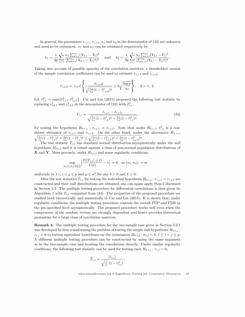
Remark 2. The multiple testing procedure for the one-sample case given in Section 3.2.1

was developed by first transforming the problem of testing the simple null hypotheses H0,i,j :

ri,j = 0 to testing equivalent hypotheses on the covariances H0,i,j : σi,j = 0, 1 ≤ i < j ≤ p.A different multiple testing procedure can be constructed by using the same argument

as in the two-sample case and treating the correlations directly. Under similar regularity

conditions, the following test statistic can be used for testing each H0,i,j : ri,j = 0,

Ti,j =|ri,j |√

κn

(1− r2i,j)

,


where κ = 13p

∑pi=1

n∑n

k=1(Xk,i−Xi)4

(∑n

k=1(Xk,i−Xi)2)2

is an estimate of κ ≡ 13

E(Xi−µi)4

[E(Xi−µi)2]2. It can be shown

that the asymptotic null distribution of Ti,j is standard normal. This combined with the

same second step leads to a multiple testing procedure that controls the FDP and FDR.

Remark 3. As in the one-sample case, the normal approximation is suitable in the two-

sample setting when the sample sizes are large. A similar bootstrap procedure can be used

to improve the accuracy of the approximation when the sample sizes are small. See Cai and

Liu (2015) for more details.

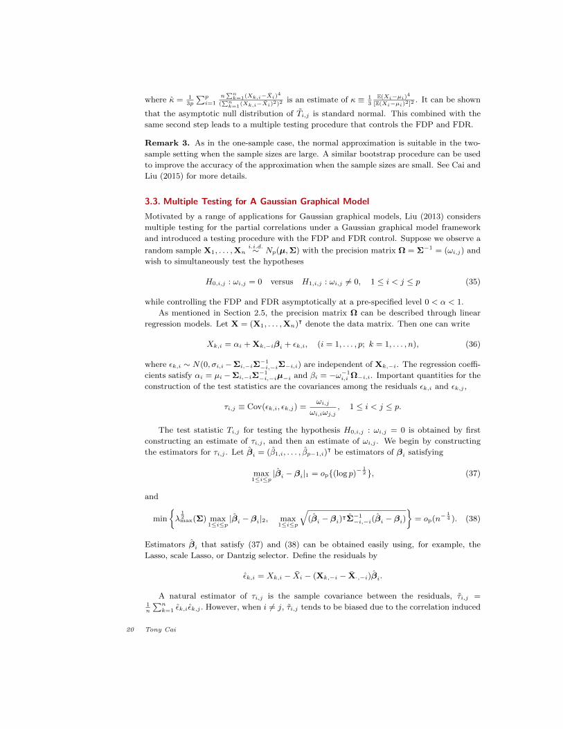
3.3. Multiple Testing for A Gaussian Graphical Model

Motivated by a range of applications for Gaussian graphical models, Liu (2013) considers

multiple testing for the partial correlations under a Gaussian graphical model framework

and introduced a testing procedure with the FDP and FDR control. Suppose we observe a

random sample X1, . . . ,Xni.i.d.∼ Np(µ,Σ) with the precision matrix Ω = Σ−1 = (ωi,j) and

wish to simultaneously test the hypotheses

H0,i,j : ωi,j = 0 versus H1,i,j : ωi,j 6= 0, 1 ≤ i < j ≤ p (35)

while controlling the FDP and FDR asymptotically at a pre-specified level 0 < α < 1.

As mentioned in Section 2.5, the precision matrix Ω can be described through linear

regression models. Let X = (X1, . . . ,Xn)ᵀ denote the data matrix. Then one can write

Xk,i = αi + Xk,−iβi + εk,i, (i = 1, . . . , p; k = 1, . . . , n), (36)

where εk,i ∼ N(0, σi,i−Σi,−iΣ−1−i,−iΣ−i,i) are independent of Xk,−i. The regression coeffi-

cients satisfy αi = µi−Σi,−iΣ−1−i,−iµ−i and βi = −ω−1

i,i Ω−i,i. Important quantities for the

construction of the test statistics are the covariances among the residuals εk,i and εk,j ,

τi,j ≡ Cov(εk,i, εk,j) =ωi,j

ωi,iωj,j, 1 ≤ i < j ≤ p.

The test statistic Ti,j for testing the hypothesis H0,i,j : ωi,j = 0 is obtained by first

constructing an estimate of τi,j , and then an estimate of ωi,j . We begin by constructing

the estimators for τi,j . Let βi = (β1,i, . . . , βp−1,i)ᵀ be estimators of βi satisfying

max1≤i≤p

|βi − βi|1 = op(log p)−12 , (37)

and

min

λ

12max(Σ) max

1≤i≤p|βi − βi|2, max

1≤i≤p

√(βi − βi)

ᵀΣ−1−i,−i(βi − βi)

= op(n−

14 ). (38)

Estimators βi that satisfy (37) and (38) can be obtained easily using, for example, the

Lasso, scale Lasso, or Dantzig selector. Define the residuals by

εk,i = Xk,i − Xi − (Xk,−i − X·,−i)βi.

A natural estimator of τi,j is the sample covariance between the residuals, τi,j =1n

∑nk=1 εk,iεk,j . However, when i 6= j, τi,j tends to be biased due to the correlation induced

20 Tony Cai

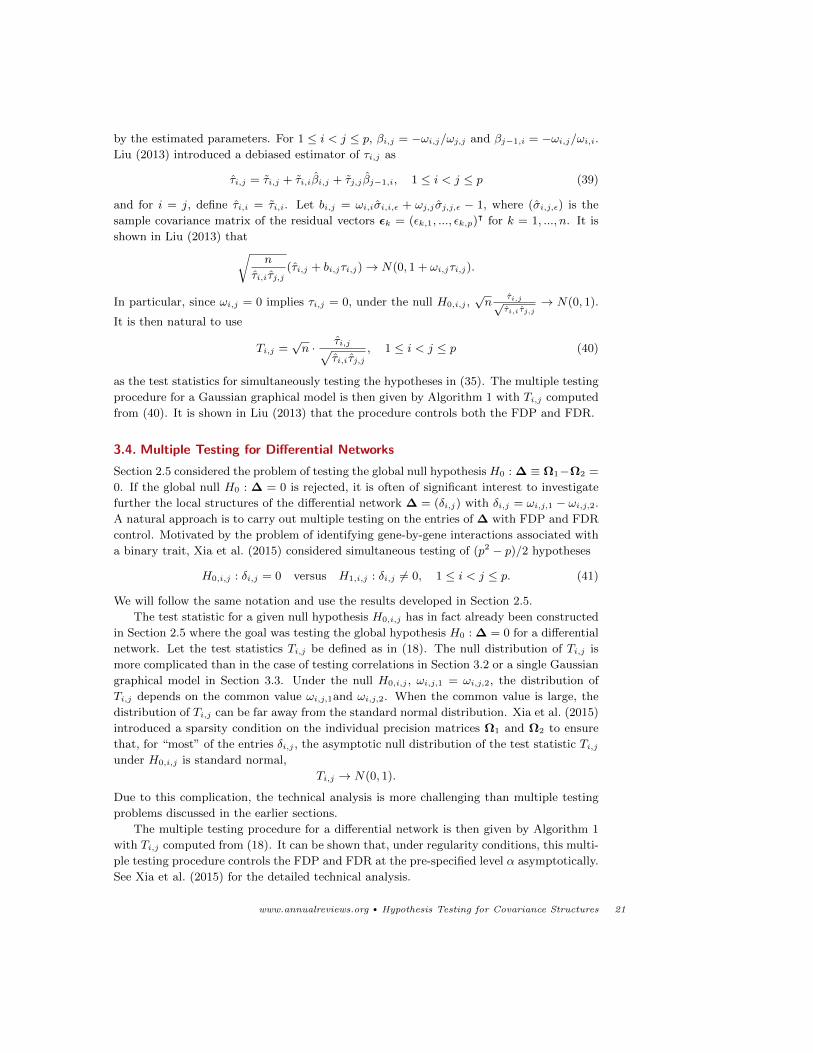
by the estimated parameters. For 1 ≤ i < j ≤ p, βi,j = −ωi,j/ωj,j and βj−1,i = −ωi,j/ωi,i.Liu (2013) introduced a debiased estimator of τi,j as

τi,j = τi,j + τi,iβi,j + τj,j βj−1,i, 1 ≤ i < j ≤ p (39)

and for i = j, define τi,i = τi,i. Let bi,j = ωi,iσi,i,ε + ωj,j σj,j,ε − 1, where (σi,j,ε) is the

sample covariance matrix of the residual vectors εk = (εk,1, ..., εk,p)ᵀ for k = 1, ..., n. It is

shown in Liu (2013) that√n

τi,iτj,j(τi,j + bi,jτi,j)→ N(0, 1 + ωi,jτi,j).

In particular, since ωi,j = 0 implies τi,j = 0, under the null H0,i,j ,√n

τi,j√τi,iτj,j

→ N(0, 1).

It is then natural to use

Ti,j =√n · τi,j√

τi,iτj,j, 1 ≤ i < j ≤ p (40)

as the test statistics for simultaneously testing the hypotheses in (35). The multiple testing

procedure for a Gaussian graphical model is then given by Algorithm 1 with Ti,j computed

from (40). It is shown in Liu (2013) that the procedure controls both the FDP and FDR.

3.4. Multiple Testing for Differential Networks

Section 2.5 considered the problem of testing the global null hypothesis H0 : ∆ ≡ Ω1−Ω2 =

0. If the global null H0 : ∆ = 0 is rejected, it is often of significant interest to investigate

further the local structures of the differential network ∆ = (δi,j) with δi,j = ωi,j,1 − ωi,j,2.

A natural approach is to carry out multiple testing on the entries of ∆ with FDP and FDR

control. Motivated by the problem of identifying gene-by-gene interactions associated with

a binary trait, Xia et al. (2015) considered simultaneous testing of (p2 − p)/2 hypotheses

H0,i,j : δi,j = 0 versus H1,i,j : δi,j 6= 0, 1 ≤ i < j ≤ p. (41)

We will follow the same notation and use the results developed in Section 2.5.

The test statistic for a given null hypothesis H0,i,j has in fact already been constructed

in Section 2.5 where the goal was testing the global hypothesis H0 : ∆ = 0 for a differential

network. Let the test statistics Ti,j be defined as in (18). The null distribution of Ti,j is

more complicated than in the case of testing correlations in Section 3.2 or a single Gaussian

graphical model in Section 3.3. Under the null H0,i,j , ωi,j,1 = ωi,j,2, the distribution of

Ti,j depends on the common value ωi,j,1and ωi,j,2. When the common value is large, the

distribution of Ti,j can be far away from the standard normal distribution. Xia et al. (2015)

introduced a sparsity condition on the individual precision matrices Ω1 and Ω2 to ensure

that, for “most” of the entries δi,j , the asymptotic null distribution of the test statistic Ti,junder H0,i,j is standard normal,

Ti,j → N(0, 1).

Due to this complication, the technical analysis is more challenging than multiple testing

problems discussed in the earlier sections.

The multiple testing procedure for a differential network is then given by Algorithm 1

with Ti,j computed from (18). It can be shown that, under regularity conditions, this multi-

ple testing procedure controls the FDP and FDR at the pre-specified level α asymptotically.

See Xia et al. (2015) for the detailed technical analysis.


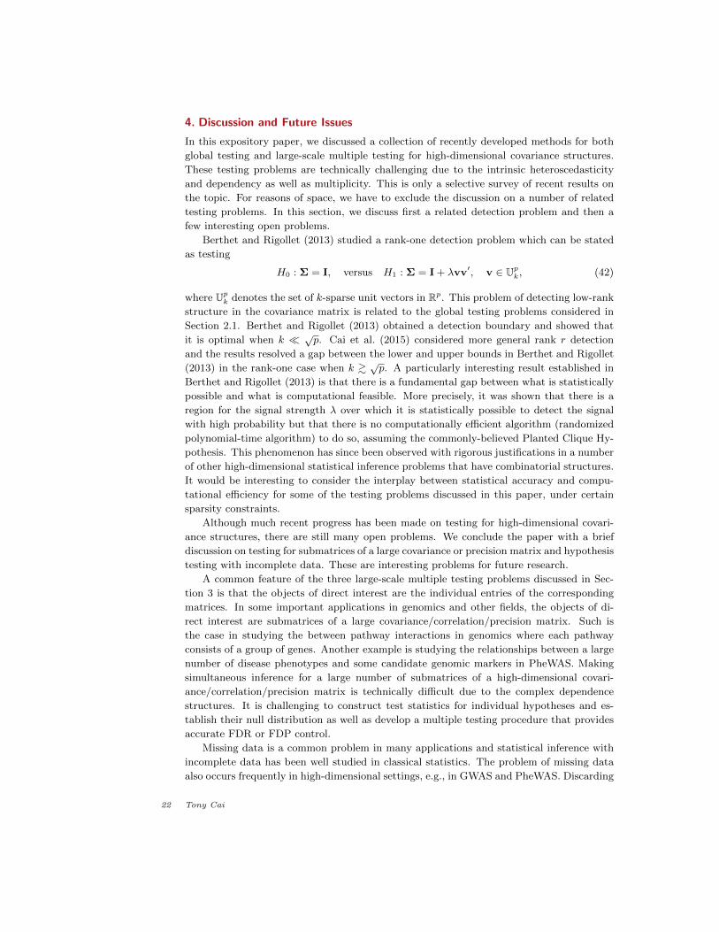
4. Discussion and Future Issues

In this expository paper, we discussed a collection of recently developed methods for both

global testing and large-scale multiple testing for high-dimensional covariance structures.

These testing problems are technically challenging due to the intrinsic heteroscedasticity

and dependency as well as multiplicity. This is only a selective survey of recent results on

the topic. For reasons of space, we have to exclude the discussion on a number of related

testing problems. In this section, we discuss first a related detection problem and then a

few interesting open problems.

Berthet and Rigollet (2013) studied a rank-one detection problem which can be stated

as testing

H0 : Σ = I, versus H1 : Σ = I + λvv′, v ∈ Upk, (42)

where Upk denotes the set of k-sparse unit vectors in Rp. This problem of detecting low-rank

structure in the covariance matrix is related to the global testing problems considered in

Section 2.1. Berthet and Rigollet (2013) obtained a detection boundary and showed that

it is optimal when k √p. Cai et al. (2015) considered more general rank r detection

and the results resolved a gap between the lower and upper bounds in Berthet and Rigollet

(2013) in the rank-one case when k &√p. A particularly interesting result established in

Berthet and Rigollet (2013) is that there is a fundamental gap between what is statistically

possible and what is computational feasible. More precisely, it was shown that there is a

region for the signal strength λ over which it is statistically possible to detect the signal

with high probability but that there is no computationally efficient algorithm (randomized

polynomial-time algorithm) to do so, assuming the commonly-believed Planted Clique Hy-

pothesis. This phenomenon has since been observed with rigorous justifications in a number

of other high-dimensional statistical inference problems that have combinatorial structures.

It would be interesting to consider the interplay between statistical accuracy and compu-

tational efficiency for some of the testing problems discussed in this paper, under certain

sparsity constraints.

Although much recent progress has been made on testing for high-dimensional covari-

ance structures, there are still many open problems. We conclude the paper with a brief

discussion on testing for submatrices of a large covariance or precision matrix and hypothesis

testing with incomplete data. These are interesting problems for future research.

A common feature of the three large-scale multiple testing problems discussed in Sec-

tion 3 is that the objects of direct interest are the individual entries of the corresponding

matrices. In some important applications in genomics and other fields, the objects of di-

rect interest are submatrices of a large covariance/correlation/precision matrix. Such is

the case in studying the between pathway interactions in genomics where each pathway

consists of a group of genes. Another example is studying the relationships between a large

number of disease phenotypes and some candidate genomic markers in PheWAS. Making

simultaneous inference for a large number of submatrices of a high-dimensional covari-

ance/correlation/precision matrix is technically difficult due to the complex dependence

structures. It is challenging to construct test statistics for individual hypotheses and es-

tablish their null distribution as well as develop a multiple testing procedure that provides

accurate FDR or FDP control.

Missing data is a common problem in many applications and statistical inference with

incomplete data has been well studied in classical statistics. The problem of missing data

also occurs frequently in high-dimensional settings, e.g., in GWAS and PheWAS. Discarding

22 Tony Cai

samples with any missingness is clearly inefficient and possibly induces bias due to non-

random missingness. It is of significant interest to develop global and multiple testing

methods for high-dimensional covariance structures in the presence of missing data.

DISCLOSURE STATEMENT

The authors are not aware of any affiliations, memberships, funding, or financial holdings

that might be perceived as affecting the objectivity of this review.

ACKNOWLEDGMENTS

The research was supported in part by NSF Grants DMS-1208982 and DMS-1403708, and

NIH Grant R01 CA127334.

LITERATURE CITED

Anderson, T. W. (2003). An Introduction to Multivariate Statistical Analysis (3rd ed.). Wiley.

Andrews, D. W. (1991). Heteroskedasticity and autocorrelation consistent covariance matrix esti-

mation. Econometrica 59, 817–858.

Bai, Z., D. Jiang, J.-F. Yao, and S. Zheng (2009). Corrections to LRT on large-dimensional covari-

ance matrix by RMT. The Annals of Statistics 37 (6B), 3822–3840.

Baik, J., G. Ben Arous, and S. Peche (2005). Phase transition of the largest eigenvalue for nonnull

complex sample covariance matrices. The Annals of Probability 33 (5), 1643–1697.

Bandyopadhyay, S., M. Mehta, D. Kuo, M.-K. Sung, R. Chuang, E. J. Jaehnig, B. Bodenmiller,

K. Licon, W. Copeland, M. Shales, D. Fiedler, J. Dutkowski, A. Guenole, H. van Attikum, K. M.

Shokat, R. D. Kolodner, W.-K. Huh, R. Aebersold, M.-C. Keogh, N. J. Krogan, and T. Ideker

(2010). Rewiring of genetic networks in response to dna damage. Sci. Signal. 330, 1385–1389.

Banerjee, O., L. El Ghaoui, and A. d’Aspremont (2008). Model selection through sparse maximum

likelihood estimation for multivariate Gaussian or binary data. The Journal of Machine Learning

Research 9, 485–516.

Benjamini, Y. and Y. Hochberg (1995). Controlling the false discovery rate: a practical and powerful

approach to multiple testing. Journal of the Royal Statistical Society. Series B (Methodologi-

cal) 57, 289–300.

Benjamini, Y. and D. Yekutieli (2001). The control of the false discovery rate in multiple testing

under dependency. Annals of statistics 29, 1165–1188.

Berthet, Q. and P. Rigollet (2013). Optimal detection of sparse principal components in high

dimension. The Annals of Statistics 41 (4), 1780–1815.

Bickel, P. J. and E. Levina (2008a). Regularized estimation of large covariance matrices. The

Annals of Statistics 36 (1), 199–227.

Bickel, P. J. and E. Levina (2008b). Covariance regularization by thresholding. The Annals of

Statistics 36 (6), 2577–2604.

Birke, M. and H. Dette (2005). A note on testing the covariance matrix for large dimension.

Statistics & Probability Letters 74 (3), 281–289.

Cai, T. T. and T. Jiang (2011). Limiting laws of coherence of random matrices with applications

to testing covariance structure and construction of compressed sensing matrices. The Annals of

Statistics 39 (3), 1496–1525.

Cai, T. T. and T. Jiang (2012). Phase transition in limiting distributions of coherence of high-

dimensional random matrices. Journal of Multivariate Analysis 107, 24–39.

Cai, T. T. and W. Liu (2011). Adaptive thresholding for sparse covariance matrix estimation.

Journal of the American Statistical Association 106 (494), 672–684.


Cai, T. T. and W. Liu (2015). Large-scale multiple testing of correlations. Journal of the American

Statistical Association 110 (to appear).

Cai, T. T., W. Liu, and X. Luo (2011). A constrained `1 minimization approach to sparse precision

matrix estimation. Journal of the American Statistical Association 106 (494), 594–607.

Cai, T. T., W. Liu, and Y. Xia (2013). Two-sample covariance matrix testing and support recovery in

high-dimensional and sparse settings. Journal of the American Statistical Association 108 (501),

265–277.

Cai, T. T., W. Liu, and H. H. Zhou (2016). Estimating sparse precision matrix: Optimal rates of

convergence and adaptive estimation. The Annals of Statistics 44, 455–488.

Cai, T. T. and Z. Ma (2013). Optimal hypothesis testing for high dimensional covariance matrices.

Bernoulli 19 (5B), 2359–2388.

Cai, T. T., Z. Ma, and Y. Wu (2013). Sparse PCA: Optimal rates and adaptive estimation. The


Cai, T. T., Z. Ma, and Y. Wu (2015). Optimal estimation and rank detection for sparse spiked

covariance matrices. Probability Theory and Related Fields 161 (3-4), 781–815.

Cai, T. T., Z. Ren, and H. H. Zhou (2013). Optimal rates of convergence for estimating Toeplitz

covariance matrices. Probability Theory and Related Fields 156 (1-2), 101–143.

Cai, T. T., Z. Ren, and H. H. Zhou (2016). Estimating structured high-dimensional covariance and

precision matrices: Optimal rates and adaptive estimation (with discussion). Electronic Journal

of Statistics 10, 1–59.

Cai, T. T. and M. Yuan (2012). Adaptive covariance matrix estimation through block thresholding.

The Annals of Statistics 40 (4), 2014–2042.

Cai, T. T. and A. Zhang (2016). Inference on high-dimensional differential correlation matrices.

Journal Multivariate Analysis 143, 107–126.

Cai, T. T., C. H. Zhang, and H. H. Zhou (2010). Optimal rates of convergence for covariance matrix

estimation. The Annals of Statistics 38 (4), 2118–2144.

Cai, T. T. and H. H. Zhou (2012). Optimal rates of convergence for sparse covariance matrix

estimation. The Annals of Statistics 40 (5), 2389–2420.

Carter, S. L., C. M. Brechbuhler, M. Griffin, and A. T. Bond (2004). Gene co-expression network

topology provides a framework for molecular characterization of cellular state. Bioinformat-

ics 20 (14), 2242–2250.

Chandrasekaran, V., P. A. Parrilo, and A. S. Willsky (2012). Latent variable graphical model

selection via convex optimization. The Annals of Statistics 40 (4), 1935–1967.

Chen, S. X., L. X. Zhang, and P. S. Zhong (2010). Tests for high-dimensional covariance matrices.


Danaher, P., P. Wang, and D. M. Witten (2014). The joint graphical lasso for inverse covariance

estimation across multiple classes. Journal of the Royal Statistical Society: Series B (Statistical

Methodology) 76 (2), 373–397.

d’Aspremont, A., O. Banerjee, and L. El Ghaoui (2008). First-order methods for sparse covariance

selection. SIAM Journal on Matrix Analysis and Applications 30 (1), 56–66.

de la Fuente, A. (2010). From “differential expression” to “differential networking” – identification

of dysfunctional regulatory networks in diseases. Trends Genet. 26 (7), 326–333.

Dubois, P. C., G. Trynka, L. Franke, K. A. Hunt, J. Romanos, A. Curtotti, A. Zhernakova, G. A.

Heap, R. Adany, A. Aromaa, et al. (2010). Multiple common variants for celiac disease influencing

immune gene expression. Nature genetics 42 (4), 295–302.

Efron, B. (2004). Large-scale simultaneous hypothesis testing: The choice of a null hypothesis.

Journal of the American Statistics Association 99, 96–104.

Efron, B. (2007). Correlation and large-scale simultaneous significance testing. Journal of the

American Statistical Association 102, 93–103.

El Karoui, N. (2007). Tracy-Widom limit for the largest eigenvalue of a large class of complex

sample covariance matrices. The Annals of Probability 35 (2), 663–714.

24 Tony Cai

El Karoui, N. (2008). Operator norm consistent estimation of large dimensional sparse covariance

matrices. The Annals of Statistics 36 (6), 2717–2756.

Fan, J., Y. Liao, and M. Mincheva (2011). High dimensional covariance matrix estimation in

approximate factor models. The Annals of Statistics 39 (6), 3320–3356.

Fan, J., Y. Liao, and M. Mincheva (2013). Large covariance estimation by thresholding principal

orthogonal complements. Journal of the Royal Statistical Society: Series B (Statistical Method-

ology) 75 (4), 603–680.

Farcomeni, A. (2007). Some results on the control of the false discovery rate under dependence.

Scandinavian Journal of Statistics 34 (2), 275–297.

Fukushima, A. (2013). Diffcorr: an r package to analyze and visualize differential correlations in

biological networks. Gene 518 (1), 209–214.

Fuller, T. F., A. Ghazalpour, J. E. Aten, T. A. Drake, A. J. Lusis, and S. Horvath (2007).

Weighted gene coexpression network analysis strategies applied to mouse weight. Mammalian

Genome 18 (6-7), 463–472.

Furrer, R. and T. Bengtsson (2007). Estimation of high-dimensional prior and posterior covariance

matrices in Kalman filter variants. Journal of Multivariate Analysis 98 (2), 227–255.

Genovese, C. and L. Wasserman (2004). A stochastic process approach to false discovery control.

The Annals of Statistics 32, 1035–1061.

Gupta, A. and J. Tang (1984). Distribution of likelihood ratio statistic for testing equality of

covariance matrices of multivariate gaussian models. Biometrika 71 (3), 555–559.

Gupta, S. D. and N. Giri (1973). Properties of tests concerning covariance matrices of normal

distributions. The Annals of Statistics 1 (6), 1222–1224.

Hirai, M. Y., K. Sugiyama, Y. Sawada, T. Tohge, T. Obayashi, A. Suzuki, R. Araki, N. Sakurai,

H. Suzuki, K. Aoki, et al. (2007). Omics-based identification of arabidopsis myb transcription

factors regulating aliphatic glucosinolate biosynthesis. Proceedings of the National Academy of

Sciences 104 (15), 6478–6483.

Huang, J. Z., N. Liu, M. Pourahmadi, and L. Liu (2006). Covariance matrix selection and estimation

via penalised normal likelihood. Biometrika 93 (1), 85–98.

Hudson, N. J., A. Reverter, and B. P. Dalrymple (2009). A differential wiring analysis of expression

data correctly identifies the gene containing the causal mutation. PLoS Comput. Biol. 5 (5),

e1000382.

Ideker, T. and N. Krogan (2012). Differential network biology. Mol. Syst. Biol. 8 (1), 565.

Jiang, D., T. Jiang, and F. Yang (2012). Likelihood ratio tests for covariance matrices of high-

dimensional normal distributions. Journal of Statistical Planning and Inference 142 (8), 2241–

2256.

Jiang, T. (2004). The asymptotic distributions of the largest entries of sample correlation matrices.

The Annals of Applied Probability 14 (2), 865–880.

John, S. (1971). Some optimal multivariate tests. Biometrika 58 (1), 123–127.

Johnstone, I. M. (2001). On the distribution of the largest eigenvalue in principal component

analysis. The Annals of Statistics 29 (2), 295–327.

Johnstone, I. M. and A. Y. Lu (2009). On consistency and sparsity for principal components analysis

in high dimensions. Journal of the American Statistical Association 104 (486), 682–693.

Lam, C. and J. Fan (2009). Sparsistency and rates of convergence in large covariance matrix

estimation. The Annals of Statistics 37 (6B), 4254–4278.

Lauritzen, S. L. (1996). Graphical Models. Oxford: Oxford University Press.

Ledoit, O. and M. Wolf (2002). Some hypothesis tests for the covariance matrix when the dimension

is large compared to the sample size. The Annals of Statistics 30 (4), 1081–1102.

Lee, H. K., A. K. Hsu, J. Sajdak, J. Qin, and P. Pavlidis (2004). Coexpression analysis of human

genes across many microarray data sets. Genome research 14 (6), 1085–1094.

Li, J. and S. X. Chen (2012). Two sample tests for high-dimensional covariance matrices. The



Li, K.-C., A. Palotie, S. Yuan, D. Bronnikov, D. Chen, X. Wei, O.-W. Choi, J. Saarela, and

L. Peltonen (2007). Finding disease candidate genes by liquid association. Genome Biol. 8 (10),

R205.

Ligeralde, A. V. and B. W. Brown (1995). Band covariance matrix estimation using restricted

residuals: A monte carlo analysis. International Economic Review 36, 751–767.

Liu, W. (2013). Gaussian graphical model estimation with false discovery rate control. The Annals

of Statistics 41 (6), 2948–2978.

Liu, W. and Q.-M. Shao (2014). Phase transition and regularized bootstrap in large-scale t-tests

with false discovery rate control. The Annals of Statistics 42 (5), 2003–2025.

Meinshausen, N. and P. Buhlmann (2006). High dimensional graphs and variable selection with the

Lasso. The Annals of Statistics 34 (3), 1436–1462.

Muirhead, R. J. (1982). Aspects of Multivariate Statistical Theory. Wiley, New York.

Nagao, H. (1973). On some test criteria for covariance matrix. The Annals of Statistics 1 (4),

700–709.

Onatski, A., M. Moreira, and M. Hallin (2013). Asymptotic power of sphericity tests for high-

dimensional data. The Annals of Statistics 41 (3), 1204–1231.

Paul, D. (2007). Asymptotics of sample eigenstructure for a large dimensional spiked covariance

model. Statistica Sinica 17 (4), 1617.

Peche, S. (2009). Universality results for the largest eigenvalues of some sample covariance matrix

ensembles. Probability Theory and Related Fields 143 (3-4), 481–516.

Perlman, M. D. (1980). Unbiasedness of the likelihood ratio tests for equality of several covariance

matrices and equality of several multivariate normal populations. The Annals of Statistics 8,

247–263.

Qiu, X., L. Klebanov, and A. Yakovlev (2005). Correlation between gene expression levels and lim-

itations of the empirical bayes methodology for finding differentially expressed genes. Statistical

Applications in Genetics and Molecular Biology 4 (1).

Qiu, Y. and S. X. Chen (2012). Test for bandedness of high-dimensional covariance matrices and

bandwidth estimation. The Annals of Statistics 40 (3), 1285–1314.

Raizada, R. D., T. L. Richards, A. Meltzoff, and P. K. Kuhl (2008). Socioeconomic status predicts

hemispheric specialisation of the left inferior frontal gyrus in young children. Neuroimage 40 (3),

1392–1401.

Ravikumar, P., M. J. Wainwright, G. Raskutti, and B. Yu (2011). High-dimensional covariance esti-

mation by minimizing `1 penalized log-determinant divergence. Electronic Journal of Statistics 5,

935–980.

Ren, Z., T. Sun, C.-H. Zhang, and H. H. Zhou (2015). Asymptotic normality and optimalities in

estimation of large Gaussian graphical model. The Annals of Statistics 43 (3), 991–1026.

Rothman, A. J., P. J. Bickel, E. Levina, and J. Zhu (2008). Sparse permutation invariant covariance

estimation. Electronic Journal of Statistics 2, 494–515.

Rothman, A. J., E. Levina, and J. Zhu (2009). Generalized thresholding of large covariance matrices.


Schott, J. R. (2007). A test for the equality of covariance matrices when the dimension is large

relative to the sample sizes. Computational Statistics & Data Analysis 51 (12), 6535–6542.

Shao, Q.-M. and W.-X. Zhou (2014). Necessary and sufficient conditions for the asymptotic distri-

butions of coherence of ultra-high dimensional random matrices. The Annals of Probability 42 (2),

623–648.

Shaw, P., D. Greenstein, J. Lerch, L. Clasen, R. Lenroot, N. Gogtay, A. Evans, J. Rapoport,

and J. Giedd (2006). Intellectual ability and cortical development in children and adolescents.

Nature 440 (7084), 676–679.

Shedden, K. and J. Taylor (2005). Differential correlation detects complex associations between

gene expression and clinical outcomes in lung adenocarcinomas. In Methods of Microarray Data

Analysis, pp. 121–131. Springer.

26 Tony Cai

Soshnikov, A. (2002). A note on universality of the distribution of the largest eigenvalues in certain

sample covariance matrices. Journal of Statistical Physics 108 (5-6), 1033–1056.

Srivastava, M. S. (2005). Some tests concerning the covariance matrix in high dimensional data.

Journal of the Japan Statistical Society 35 (2), 251–272.

Srivastava, M. S. and H. Yanagihara (2010). Testing the equality of several covariance matrices with

fewer observations than the dimension. Journal of Multivariate Analysis 101 (6), 1319–1329.

Storey, J., J. Taylor, and D. Siegmund (2004). Strong control, conservative point estimation, and

simultaneous conservative consistency of false discovery rates: A unified approach. Journal of

the Royal Statistical Society, Series B 66, 187–205.

Storey, J. D. (2002). A direct approach to false discovery rates. Journal of the Royal Statistical

Society, Series B 64, 479–498.

Sugiura, N. and H. Nagao (1968). Unbiasedness of some test criteria for the equality of one or two

covariance matrices. The Annals of Mathematical Statistics 39 (5), 1686–1692.

Sun, T. and C.-H. Zhang (2013). Sparse matrix inversion with scaled Lasso. The Journal of Machine

Learning Research 14 (1), 3385–3418.

Sun, W. and T. T. Cai (2007). Oracle and adaptive compound decision rules for false discovery

rate control. Journal of the American Statistical Association 102, 901–912.

Sun, W. and T. T. Cai (2009). Large-scale multiple testing under dependence. Journal of the Royal

Statistical Society: Series B 71, 393–424.

Sun, W., B. J. Reich, T. T. Cai, M. Guindani, and A. Schwartzman (2015). False discovery control

in large-scale spatial multiple testing. Journal of the Royal Statistical Society: Series B 77,

59–83.

Vu, V. Q. and J. Lei (2013). Minimax sparse principal subspace estimation in high dimensions. The


Wu, W. B. (2008). On false discovery control under dependence. The Annals of statistics, 364–380.

Wu, W. B. and M. Pourahmadi (2009). Banding sample autocovariance matrices of stationary

processes. Statistica Sinica 19 (4), 1755–1768.

Xia, Y., T. Cai, and T. T. Cai (2015). Testing differential networks with applications to detecting

gene-by-gene interactions. Biometrika 102, 247–266.

Xiao, H. and W. B. Wu (2011). Simultaneous inference of covariances. arXiv preprint

arXiv:1109.0524 .

Yuan, M. (2010). Sparse inverse covariance matrix estimation via linear programming. The Journal

of Machine Learning Research 11, 2261–2286.

Yuan, M. and Y. Lin (2007). Model selection and estimation in the Gaussian graphical model.

Biometrika 94 (1), 19–35.

Zhang, J., J. Li, and H. Deng (2008). Class-specific correlations of gene expressions: identification

and their effects on clustering analyses. The American Journal of Human Genetics 83 (2), 269–

277.

Zhao, S. D., T. T. Cai, and H. Li (2014). Direct estimation of differential networks. Biometrika 101,

253–268.

Zheng, S., Z. Bai, and J. Yao (2015). Substitution principle for CLT of linear spectral statistics of

high-dimensional sample covariance matrices with applications to hypothesis testing. The Annals

of Statistics 43 (2), 546–591.

Zhu, D., A. O. Hero, Z. S. Qin, and A. Swaroop (2005). High throughput screening of co-expressed

gene pairs with controlled false discovery rate (fdr) and minimum acceptable strength (mas).

Journal of Computational Biology 12 (7), 1029–1045.

Zou, H., T. Hastie, and R. Tibshirani (2006). Sparse principal component analysis. Journal of

Computational and Graphical Statistics 15 (2), 265–286.


global testing and testing for high-dimensional …tcai/paper/testing...1.1.global testing for...

Documents