Policy Research Working Paper 7536

Global Supply Chains and Trade PolicyEmily J. Blanchard

Chad P. BownRobert C. Johnson

Development Research GroupTrade and International Integration TeamJanuary 2016

WPS7536P

ublic

Dis

clos

ure

Aut

horiz

edP

ublic

Dis

clos

ure

Aut

horiz

edP

ublic

Dis

clos

ure

Aut

horiz

edP

ublic

Dis

clos

ure

Aut

horiz

ed

Produced by the Research Support Team

Abstract

The Policy Research Working Paper Series disseminates the findings of work in progress to encourage the exchange of ideas about development issues. An objective of the series is to get the findings out quickly, even if the presentations are less than fully polished. The papers carry the names of the authors and should be cited accordingly. The findings, interpretations, and conclusions expressed in this paper are entirely those of the authors. They do not necessarily represent the views of the International Bank for Reconstruction and Development/World Bank and its affiliated organizations, or those of the Executive Directors of the World Bank or the governments they represent.

Policy Research Working Paper 7536

This paper is a product of the Trade and International Integration Team, Development Research Group. It is part of a larger effort by the World Bank to provide open access to its research and make a contribution to development policy discussions around the world. Policy Research Working Papers are also posted on the Web at http://econ.worldbank.org. The authors may be contacted at cbown@worldbank.org.

How do global supply chain linkages modify countries’ incentives to impose import protection? Are these link-ages empirically important determinants of trade policy? To address these questions, this paper introduces supply chain linkages into a workhorse terms-of-trade model of trade policy with political economy. Theory predicts that discretionary final goods tariffs will be decreasing in the domestic content of foreign-produced final goods. Pro-vided foreign political interests are not too strong, final

goods tariffs will also be decreasing in the foreign content of domestically-produced final goods. The paper tests these predictions using newly assembled data on bilateral applied tariffs, temporary trade barriers, and value-added contents for 14 major economies over the 1995–2009 period. There is strong support for the empirical predictions of the model. The results imply that global supply chains matter for trade policy, both in principle and in practice.

Global Supply Chains and Trade Policy∗

Emily J. Blanchard† Chad P. Bown‡ Robert C. Johnson§

January 2016

Keywords Global Supply Chains, Tariffs, Temporary Trade Barriers, Trade Agreements

JEL Codes F1, F13, F14, F23, F68

∗We thank Thibault Fally, Nuno Limao, Ralph Ossa, Raymond Robertson, and Robert Staiger for feed-back on early drafts. We also thank seminar participants at Berkeley (ARE), Columbia, ETH Zurich,Harvard, Yale, the USITC, the Dartmouth/SNU Workshop on International Trade Policy and Institutions,the CEPR/ECARES/CAGE Global Fragmentation of Production and Trade Policy Workshop, the ThirdIMF/WB/WTO Joint Trade Workshop, the 2015 AEA Annual Meetings, the 2015 NBER ITI Spring Meet-ings, the 2015 EIIT Conference, and the 2015 Southern Economic Association Meetings for helpful comments.Bown acknowledges financial support from the World Bank’s Multi-Donor Trust Fund for Trade and Devel-opment. Carys Golesworthy provided outstanding research assistance.†Tuck School of Business at Dartmouth; emily.blanchard@tuck.dartmouth.edu‡World Bank and CEPR; cbown@worldbank.org§Dartmouth College and NBER; robert.c.johnson@dartmouth.edu

In the modern global economy, final goods are typically produced by combining domestic

and foreign value added via global supply chains. Foreign value added accounts for 20 percent

of the value of final manufacturing output in many countries, and more than 50 percent in

some countries and sectors. In turn, imported final goods contain substantial domestic value

added, as exported intermediate inputs return home embodied in foreign-made final goods.

These global supply chain linkages alter the conventional calculus of import protection.

First, taxing imports hurts those upstream domestic firms that supply inputs to foreign

producers, because import barriers depress the value of foreign goods produced and hence

revenue accruing to domestic input suppliers. This mechanism dampens governments’ in-

centives to impose import protection. Second, when domestic final goods firms use foreign

value added in production, some of the benefits of an import tariff are passed back through

the supply chain to foreign input suppliers. This too discourages import protection.

Despite these observations, global supply chains are absent in most theoretical and empir-

ical analysis of trade policy. This omission is conspicuous in light of the growing importance

of global supply chains as conduits of trade. It is also out of step with ongoing discussions

among trade policymakers, in which supply chain concerns are front and center.1

In this paper, we introduce cross-border supply chain linkages into a workhorse terms-of-

trade model of trade policy. We use the model to characterize how government objectives over

final goods tariffs depend on the nationality of the value-added content embodied in home

and foreign final goods. Using newly assembled data on bilateral applied tariffs, temporary

trade barriers (TTBs), and value-added contents, we then test the predictions of the model

for 14 major economies over the 1995-2009 period. We find strong support for the empirical

predictions of the model: by erasing the distinction between final goods made at home versus

made abroad, global supply chains are reshaping trade policy.

Our framework and results contribute to both the theoretical and empirical trade policy

literatures. The first theoretical contribution is to extend the canonical terms-of-trade the-

ory to include cross-border supply chain linkages. In our model, final goods are produced by

combining domestic and foreign value added (equivalently, home and foreign primary fac-

tors). The use of foreign value added in production drives a wedge between national income

and the value of final goods production in each country: some revenue from domestic final

goods production ultimately accrues to foreigners, while some foreign final goods revenue

is paid to home residents. This re-conceptualization of the production process changes the

mapping from prices to income, and hence welfare, relative to standard models. As a result,

global supply chains alter government incentives to apply import protection.

1On the role of supply chains in policy discussions, see the WTO’s Made in the World Initiative and the2014 World Trade Report [WTO (2014)]. See also Baldwin (2012) and Hoekman (2014).

1

As a second theoretical contribution, we embed this mechanism in a many-country, many-

good framework with political economy motives to study optimal bilateral trade policy. We

first derive unilaterally optimal bilateral tariffs for final goods, and then we describe how

bilateral tariffs differ when they are set via reciprocal trade agreements (RTAs).

Starting with unilateral policy, the optimal tariff deviates from the standard “inverse

export supply elasticity rule” for three reasons. First, domestic content embodied in foreign

final goods dampens a country’s incentive to manipulate its terms of trade. Put simply,

tariffs push down the prices that foreign producers receive, which hurts upstream domestic

producers who supply value added to foreign producers. Thus, all else equal, a country will

set lower tariffs against imports that embody more of its own domestic value-added content.

Through a second channel, foreign content embodied in domestic final goods also reduces

the government’s incentive to impose tariffs. Intuitively, when import-competing sectors use

foreign inputs, some protectionist rents from higher tariffs accrue to foreign upstream sup-

pliers. This mechanism also reduces the government’s incentive to apply import protection.

Importantly, this effect of foreign value-added content on tariffs arises even if the government

has no ability (or motive) to manipulate its terms of trade; this channel thus constitutes a

distinct international externality, which we refer to as the domestic-price externality.

Political economy (distributional) concerns are a third source of deviations from the

inverse elasticity rule. If the government affords additional political weight to domestic

suppliers of value added embodied in foreign final goods, the tariff liberalizing effect via

the first channel will be stronger. Conversely, if the government affords political weight to

the interests of foreign suppliers of value added embodied in domestic goods, these political

concerns may weaken (or even overturn) the second channel. Finally, if the government favors

domestic producers of final goods, politically optimal tariffs also rise. Though familiar, this

last point is important for taking the theory to data.

Recognizing that some tariff preferences are determined under the auspices of bilateral

trade agreements, we extend our analysis to allow for reciprocity in bilateral tariff setting.

We show that tariffs inside reciprocal agreements respond differently to value-added con-

tent than do tariff preferences set outside reciprocal agreements. Specifically, if reciprocity

neutralizes terms-of-trade externalities among parties to the trade agreement [Bagwell and

Staiger (1999)], then tariffs set via reciprocal agreements will be insensitive to the amount

of domestic value added in foreign goods. In contrast, foreign value added in domestic pro-

duction will influence even reciprocally-negotiated tariffs, since foreign value added shapes

tariffs via the domestic-price externality rather than through the terms of trade.

Our study of the effect of global supply chains on trade policy connects with two strands

of related theoretical work. First, it complements Antras and Staiger (2012), who analyze

2

how bilateral bargaining among supply chain partners alters the mapping from tariffs to

prices, and therefore optimal trade policy. In contrast to their approach, we are agnostic

about the nature of price determination within global supply chains; our results obtain even

if prices are determined by market clearing conditions, as in conventional models. Our

work also builds on Blanchard (2007, 2010), who shows that foreign direct investment and

international ownership alter the standard mapping from prices to income, and thus optimal

tariffs. Though similar in spirit, the mechanics and empirical implications of the model in

this paper are different. Our theory links observable input trade patterns to bilateral tariffs,

separate from ownership concerns.

Turning to the empirics, our first contribution is that we combine data on bilateral im-

port protection and value-added contents to test key predictions of the theory. We focus

our analysis on dimensions of policy over which governments have scope to implement dis-

cretionary levels of protection.2 We first examine bilateral applied tariffs, where countries

offer preferential tariffs to selected partners. We then examine the use of temporary trade

barriers (antidumping, safeguards, and countervailing duties) in a separate, complementary

set of exercises.

Our approach to analyzing bilateral tariffs is guided by both the theory and key in-

stitutional features that govern tariff setting in practice. Theory motivates the empirical

specifications we adopt and our choice of controls. In a first specification, we focus on identi-

fying the role of domestic value added in foreign production, using fixed effects to control for

export supply elasticities, political economy, and foreign value-added effects. We then turn

to a second theory-based specification to identify the role of foreign value added in domestic

production. Throughout the analysis, we measure value-added contents using input-output

methods and data from the World Input-Output Database.

Because institutional features of the multilateral trading system constrain policy, we are

careful to incorporate them into our empirical strategy. While governments have discretion to

offer preferential tariffs bilaterally via various trade preference programs (under the GATT’s

Article XXIV or Enabling Clause), they are subject to several relevant constraints. The first

is the most-favored-nation (MFN) rule under the GATT, which caps bilateral tariffs for many

trading partners at levels below the unilaterally optimal tariff. The implication is that we can

observe bilateral optimal tariffs up to, but not above, the MFN threshold. We use non-linear

methods to address this partial non-observability, or censoring, problem in the estimation.

A second constraint is that some bilateral tariffs are set via reciprocal trade agreements. As

2Our study is in the tradition of earlier work examining unconstrained dimensions of policy, includingTrefler (1993), Goldberg and Maggi (1999), Gawande and Krishna (2003), Broda, Limao and Weinstein(2008), Bown and Crowley (2013), and Blanchard and Matschke (2015), among others.

3

noted earlier, theory predicts that the domestic value-added content of foreign goods plays

a different role inside versus outside reciprocal agreements, and accordingly we examine this

prediction in the data. Together, these strategies constitute a new approach to examining

bilateral trade policy data, which can be used to address many trade policy questions beyond

this paper.

Summarizing our results, we first find that higher domestic value added in foreign final

goods results in lower applied bilateral tariffs. This result holds across alternative specifi-

cations that control for confounding factors using both observable proxies and fixed effects.

Consistent with the theory, this liberalizing effect of domestic value added holds for tar-

iffs set under non-reciprocal preference programs, but not for reciprocal tariff preferences.

Moreover, the estimated influence of domestic value added on tariffs becomes stronger when

we instrument for domestic value-added content and correct for censoring. Second, we find

that higher foreign value added in domestic final goods results in lower applied bilateral

tariffs. This effect again strengthens when we correct for censoring and holds most strongly

inside reciprocal trade agreements, where reciprocity does not neutralize the domestic-price

externality.

Finally, we show that bilateral TTB coverage ratios respond to value-added content in

much the same way as bilateral applied tariffs. These results both corroborate our findings

for tariffs and extend our analysis to include these increasingly important discretionary

trade policy instruments. Furthermore, we find the role of domestic value added in foreign

production to be strongest for TTB-use against China, where antidumping and other TTBs

were most actively deployed during the 1995-2009 period.

In addition to highlighting the role of global supply chains, our empirical results con-

tribute to the existing trade policy literature in several other ways. Our evidence linking

the domestic value-added content in foreign production to bilateral tariffs fits into an impor-

tant literature documenting that terms-of-trade concerns matter for trade policy formulation

[Broda, Limao and Weinstein (2008), Bagwell and Staiger (2011), Ludema and Mayda (2013),

Bown and Crowley (2013)]. To our knowledge, we are the first to demonstrate the relevance

of the theory for bilateral tariff policy.3 Along the way, we take care to distinguish the pre-

dictions of the theory inside versus outside RTAs. We are also the first (to our knowledge)

to document that tariffs set via reciprocal bilateral trade agreements behave in a manner

consistent with the neutralization of terms-of-trade motives.

This paper also contributes to a recent literature that applies input-output methods to

3In this, our work complements Bown and Crowley (2013), who document the importance of terms-of-trade influences in US application of bilateral antidumping and safeguard measures, and Blanchard andMatschke (2015), who show that the United States is more likely to offer preferential market access todestinations that host US multinational affiliates that sell goods back to the US.

4

measure the value-added content of trade [Johnson and Noguera (2012), Koopman, Wang

and Wei (2014), Los, Timmer and de Vries (2015)]. Drawing on this work, we examine the

implications of value-added contents for a particular set of economic policies.

The paper proceeds as follows. Section 1 presents the theoretical framework. Section 2

outlines our empirical strategy for taking the theory to data. Section 3 describes the data.

Sections 4 and 5 include the empirical results, and Section 6 concludes.

1 Theoretical Framework

This section develops a many-country, many-good, political-economy model in which value-

added content influences the structure of bilateral tariffs on final goods. We open with a

general discussion of our modeling choices, then proceed to the formal characterization of

optimal tariffs.

1.1 Modeling Tariff Preferences

Building on existing trade policy models, we design our theoretical framework to respect

the institutional context in which bilateral trade policy is set. We dedicate special attention

to two institutional issues that figure prominently in our empirical investigation: the most-

favored-nation (MFN) rule and the role of reciprocity in bilateral trade agreements.

The MFN Rule The most-favored-nation rule dictates that WTO members may not dis-

criminate across their WTO-member trading partners, but for defined exceptions to this rule.

Further, MFN-exceptions defined under the GATT’s Article XXIV and Enabling Clauses al-

low downward deviations from MFN only – i.e., countries may offer tariff preferences, but

they may not impose higher-than-MFN discriminatory tariffs. As a result, MFN tariff rates

serve as an upper bound on applied bilateral tariffs.

In our model, we analyze how discriminatory bilateral tariffs respond to value-added

content, given this MFN constraint. In doing so, we take MFN tariffs as given. This

assumption follows Grossman and Helpman (1995a), who also take MFN tariffs as given

when analyzing politically-optimal bilateral trade agreements.4

4To justify this assumption, Grossman and Helpman (1995a) appeal to GATT Article XXIV, which pro-hibits countries that adopt bilateral agreements from raising their external (MFN) tariffs. Further consistentwith this assumption, existing theoretical and empirical work finds that tariff preferences have an ambigu-ous impact on MFN tariffs. See Bagwell and Staiger (1997), McLaren (2002), Saggi (2009) for theoreticalanalysis. On the empirics, Limao (2006) finds that tariff preferences make subsequent MFN liberalizationless likely, while Estevadeordal, Freund and Ornelas (2008) find the opposite.

5

More pertinent to our empirical application, there are two additional rationales for fo-

cusing on bilateral deviations from MFN, rather than MFN tariffs themselves. First, current

MFN tariffs were largely set under the Uruguay Round, which was completed in 1994.5 Not

only does this predate our sample period, but the MFN negotiations also largely predated

the post-1990 rise in global supply chain activity. In contrast, bilateral tariff preferences are

an active area of trade policy during the 1995-2009 period, and thus a more fertile ground for

empirical exploration. Second, the empirical framework that we develop exploits variation

in tariff preferences across trade partners within a given importer and industry. Thus, we

effectively difference away MFN tariffs (and their multilateral determinants) in all of our

empirical specifications.

Reciprocity While the the majority of observed bilateral preferences in our data are uni-

lateral (non-reciprocal) in nature, some are the result of free trade agreements or customs

unions, permitted under GATT Article XXIV. Because these agreements are the result of

comprehensive negotiations between partner countries, tariff reciprocity may (at least in

part) neutralize bilateral terms-of-trade externalities [Grossman and Helpman (1995b), Bag-

well and Staiger (1999)]. Accordingly, we take care to analyze reciprocal trade preferences

separately from non-reciprocal preferences. We first derive optimal bilateral tariffs under the

assumption that preferences are set unilaterally. We then re-derive optimal tariffs under the

assumption that they are set cooperatively, as in a reciprocal trade agreement.

Additional Model Background To facilitate presentation of the main ideas, we make

a number of additional technical assumptions. We focus on a tractable partial equilibrium

setting with a numeraire sector, quasi-linear preferences, and sector-location specific factors

of production. This set up isolates the direct determinants of trade policy, separate from

potential general equilibrium contaminants.6 To simplify the exposition, we also take as given

the quantities of the specific factors used in production, as is standard in the literature. In

Appendix A, we demonstrate that the key theoretical mechanisms and empirical predictions

are unchanged if we instead allow these quantities to be endogenous.

In the background, our model also implicitly takes input tariffs as given.7 The logic

5This is true for industrialized countries. As a legacy of the Uruguay round, MFN tariffs for these countriessometimes fall during our sample period due to extended phase-in schedules. Although MFN tariffs for severalemerging markets were lowered during our sample period, either unilaterally or in conjunction with joiningthe WTO, our empirical strategy ensures that these MFN tariff changes do not drive the results.

6This approach follows Grossman and Helpman (1994), Broda, Limao and Weinstein (2008), Ludema andMayda (2013) and many others.

7We also set aside the question of how value-added trade might affect optimal export policy, in keepingwith both the existing literature and institutional limits. GATT rules prohibit export subsidies, and exporttaxes are seldom used and, in the US, even unconstitutional.

6

for doing is as follows. Input tariffs alter value-added content by changing input prices

and/or sourcing decisions. Therefore, input tariffs influence final goods tariffs via value-

added contents. Given value-added contents, however, input tariffs have no additional (first

order) impact on final goods tariffs.8 Since we focus on the link between value-added content

and final goods tariffs, not the determination of value-added content, we need not address

input tariffs directly.

Finally, although the theory focuses on bilateral tariffs, import protection takes other

forms, most notably the discretionary use of upward deviations from MFN tariffs via anti-

dumping duties and related temporary trade barriers. We defer discussion about how we

extend our arguments to the TTB environment until Section 5.

1.2 Model Set-up

Consider a multi-country, multi-good setting in which every country produces and trades

potentially many final goods. The set of countries is given by C = 1, ..., C, where C may

be large. There are S + 1 final goods, where the numeraire final good is indexed by 0, and

all other (non-numeraire) goods are indexed by the set S = 1, ..., S. Final goods prices in

each country are denoted by pcs, where c designates the location and s the final goods sector.

The numeraire is freely traded, so that pc0 = 1 for all countries c ∈ C. We use ~pc = (pc1, ..., pcS)

to denote the vector of (non-numeraire) final goods prices in country c, ~ps = (p1s, ..., p

Cs ) to

denote the vector of sector s prices in each country, and ~p = (~p1, ..., ~pC) to represent the

complete (1× SC) vector of final goods prices in every country world-wide.9

Each country is populated by a continuum of identical workers with mass normalized to

one. Preferences are identical and quasi-linear, given by the aggregate utility function:

U c = dc0 +∑s∈S

us(dcs) ∀c ∈ C, (1)

where dcs represents consumption of final goods in sector s in country c and sub-utility over

the non-numeraire goods is differentiable and strictly concave. Consumption is chosen to

maximize utility subject to the budget constraint, dc0 +∑

s pcsdcs ≤ Ic, where Ic is national

8In our model, the only link between input tariffs and final goods tariffs works through tariff revenue,whereby changes in final goods tariffs may induce changes in the value of imported inputs and thus tariffrevenue. Due to our specific-factors assumption, this effect obtains only for ad-valorem tariffs. Further, thischannel is shut down when input tariffs are set to zero. In reality, input tariffs are sufficiently low that weabstract from it.

9It often proves useful to partition price vectors into domestic and foreign components [Bagwell and Staiger(1999)]. From the perspective of a given home country i, let ~p ≡ (~pi, ~p∗), where ~p∗ is the (1 × S(C − 1))vector of prices in every country other than i. Likewise, let ~ps ≡ (pis, ~p

∗s) where ~p∗s is the (1× (C − 1)) vector

of prices on s in every country other than i.

7

(aggregate) income in country c, measured in the numeraire.

Production Each country is endowed with two types of factors. The first is a homoge-

neous factor, which is perfectly mobile across sectors within each country but cannot move

across countries. The numeraire good is produced under constant returns to scale using the

homogeneous factor (e.g., undifferentiated labor), which normalizes the wage to one in all

countries. The second is a specific factor, which we refer to as “value-added inputs.”10 With

global supply chains, each country’s value-added inputs may be used in production of final

goods both at home and abroad. Further, we assume these value-added inputs are specific

to the destination country and sector in which they are used to produce final goods.

Final goods in non-numeraire sector s in country c are produced using the homogeneous

factor, domestic value-added inputs, and foreign value-added inputs:

qcs = f cs (lcs, ν

csc, ~ν

cs∗) ∀s ∈ S, c ∈ C, (2)

where qcs is quantity of final goods produced, lcs is the quantity of homogeneous factor used,

νcsc is the quantity of the home (country c) value-added input used, and ~νcs∗ is the (1× (C −1)) vector of foreign value-added inputs used by sector s in country c.11 As a notational

convention, superscripts denote the country-location of production, and subscripts denote

the production sector and country-origin of value-added inputs.

As is standard, the specific value-added inputs capture all residual profit (quasi-rents)

from production, so the prices paid to the specific value-added inputs vary endogenously

with final goods prices. The quasi-rent associated with production by sector s in country i

(πis) is given by:

πis(pis) = pisq

is(p

is)− wlis(pis) =

∑c∈C

riscνisc, (3)

where risc denotes price of value-added inputs from each country c ∈ C used in production

of s in country i. Value-added input prices risc depend on final goods output prices and the

vector of value-added inputs in production: risc ≡ risc(pis;~ν

is) ∀i, j, s.

This view of the production process and the role of global supply chains is intentionally

reduced form and captures two essential features of global supply chains. First, output is

10These value-added inputs are simply bundles of specific primary factors. One could replace the termvalue-added inputs everywhere with “specific capital” or “specific human capital” (or any other compositeof specific primary factors) and all the results go through. We prefer the value-added nomenclature becauseit is tied to what we measure in the data.

11It proves helpful to partition the (1×C) vector of value-added inputs, ~νcc , into local value-added inputs,νcsc, and the (1× (C − 1)) vector of foreign value-added inputs, denoted by an asterisk: ~νcs ≡ (νcsc, ~ν

cs∗).

8

produced using both home and foreign production factors when supply chains span borders.12

Second, global supply chain activities are characterized by high degrees of input specificity

and lock-in between buyers and suppliers, as emphasized by Antras and Staiger (2012), which

manifests itself in our model as factor specificity.13

The model captures these ideas without taking a stand on the underlying production

structure by which factors are transformed into final goods via global supply chains, and

thus without specifying the exact division of quasi-rents across the different value added

components. We assume only that the mapping from final goods prices to the vector of

quasi-rents is well-defined and can be represented by elasticity terms of the form εrisc, which

describes how changes in the price of a final good are passed through to value-added inputs.14

National Income National income equals the sum of tariff revenue and payments to the

homogeneous factor and value-added inputs:

I i = R(~p, I i;~ν) + 1 +∑s∈S

risiνisi +

∑s∈S

∑c 6=i∈C

rcsiνcsi, (4)

where tariff revenue is R(~p, I i;~ν) ≡∑

s∈S∑

c 6=i∈C(pis − pcs)M

isc(~p, I

i;~ν), M isc is country i’s

imports of good s from country c, and labor income of the homogeneous factor is 1 due to

normalization. Using (3), we can rewrite (4) as:

I i = 1 + ~pi · ~qi(~pi, ~νi) +R(~p, I i;~ν)−∑s∈S

∑c 6=i∈C

riscνisc︸ ︷︷ ︸

≡FV Ai(~pi)

+∑s∈S

∑c 6=i∈C

rcsiνcsi︸ ︷︷ ︸

≡DV Ai(~p∗)

. (5)

The first three components of Equation (5) mirror traditional models, in which national

income equals final goods output plus tariff revenue. There are two adjustments to this

standard definition of income due to global supply chain linkages. First, some of the revenue

from domestic final goods production is paid to foreign factors of production (foreign value-

added inputs). Henceforth, we refer to these payments to foreign factors as FVA, or foreign

12This technology abstracts from supply side details concerning how value-added input trade takes place. Asimple interpretation is that intermediate inputs are produced at home and shipped abroad to be assembledinto final goods. More complicated supply chains spread over multiple countries are also possible. Bothrepresentations map to Equation (2) as a reduced form.

13In Appendix A, we extend the model to relax the specific factors assumption, replacing it with assump-tions that imply value-added inputs are imperfectly substitutable in production. We show this preservesboth the key mechanisms and empirical predictions of the framework.

14Formally, let εrisc denote the elasticity of the return to country c’s value added embodied in sector sproduction in country i with respect to changes in the local price of final goods in sector s in country i.These elasticity terms will depend on various (unmodeled) supply side primitives (e.g., production structure,market frictions, market power, etc.).

9

value added in domestic final goods. Second, the home country earns income by supplying

home value-added inputs to foreigners. We refer to these payments as DVA, or domestic

value added in foreign final goods. Foreshadowing the key mechanism below, note that DVA

and FVA depend on final goods prices, via value-added input prices. Because tariffs influence

these prices, trade policy affects income in a non-standard way in our model.

Political Economy We assume the government’s objective function is given by the sum

of national income, consumer surplus, and the weighted sum of quasi-rents in production:

Gi = I i + ζ(~pi) +∑s

[δisπis(p

is) + δis∗FV A

is(p

is) + δ∗siDV Asi(~p

∗s)], (6)

where ζ(~pi) ≡∑

s[us(ds)− pisds] is consumer surplus and δis, δis∗, δ∗si are political economy

weights (relative to aggregate welfare) attached to various sources of rents.

This objective function augments standard political economy assumptions to recognize

the potential political influence of foreign and domestic supply chain interests. The first two

terms measure the indirect utility of the representative consumer (aggregate welfare). The

remaining terms capture political economy influences: δis is the weight that the government

puts on total rents from domestic final goods production, δis∗ is the weight placed on rents

from domestic production that accrue to foreign value-added inputs (FV Ais), and δ∗si is the

weight placed on rents accruing to domestic value-added inputs used in foreign final goods

production (DV Asi). We do not impose a priori restrictions on the weights, but standard

arguments would imply positive values for politically active constituencies.15

1.3 Optimal Bilateral Tariffs

We are now ready to characterize unilaterally optimal bilateral tariffs. Given the partial

equilibrium setting, we can characterize optimal bilateral tariffs one good at a time, as each

is independent of the other goods’ prices or tariffs.

15These weights reflect a range political economy forces. The restriction δis = δis∗ = δ∗si = 0 yields a nationalwelfare maximizing government. Standard protection-for-sale lobbying would imply δix > 0 for a politicallyactive industry [Grossman and Helpman (1994)]. Similarly, δ∗xi would be positive if domestic value-addedinput suppliers advocate for better market access on behalf of their foreign downstream buyers. To theextent that the government responds to the interests of foreign value-added input suppliers, δis∗ would alsobe positive. For instance, foreigners could lobby directly over trade policy [Gawande, Krishna and Robbins(2006)]. Alternatively, foreign value-added inputs suppliers could be represented in domestic politics by theirdownstream buyers, as in tariff jumping foreign investors that earn political goodwill [Bhagwati et al. (1987)]and advocate on behalf of their upstream affiliates located abroad. Finally, we implicitly assume that thehome government affords zero consideration to foreign value-added inputs in foreign production, though thisassumption could also easily be relaxed.

10

Country i’s optimal tariff on final goods in sector x against a given trading partner j ∈ Cmaximizes Equation (6) subject to two constraints. The first is a standard no arbitrage

condition: pix = τ ixjpjx, where τ ≡ (1 + tixj) and tixj is the ad valorem tariff. The second is

the MFN rule, as discussed earlier. Letting ti,MFNx denote the MFN tariff, then the MFN

rule implies that ti,applied

xj ≤ ti,MFNx , where ti,applied

xj is the bilateral applied tariff. Given the

allocation of specific value-added inputs, every other country’s tariff schedules, and its own

MFN tariffs, country i’s unilaterally optimal tariff on imported good x from country j is

given by:

τ ixj = arg max Gi s.t. pix = τ ixjpjx and τ ixj ≤ τ i,MFN

x . (7)

If the optimal tariff is unconstrained, then it solves the following first order condition:

Giτ ixj

=dM i

x

dτ ixjtixjp

jx−M i

xj

dpjxdτ ixj

+δixqix

dpixdτ ixj

+ΩRixj−(1−δix∗)

dFV Aixdτ ixj

+(1+δ∗xi)dDV Axidτ ixj

= 0. (8)

The first two terms of this expression capture the standard terms-of-trade motive, and

the third term represents the (familiar) effect of domestic protectionist political pressure.16

The term ΩRixj ≡

∑c6=i,j

dRixcdτ ixj

captures the potential for trade diversion to change country

i’s tariff revenue from trade with countries other than j.17 The last two terms capture the

politically-weighted influence of trade in value-added inputs on the optimal tariff.

Consider first the role of foreign value added embodied in domestic final goods (FVA).

The bilateral tariff raises the local final goods price (pix), which in turn increases the returns

to foreign value-added inputs embodied in domestic production (rixc(pix)). We decompose

this effect as follows:

dFV Aixdτ ixj

=∑c 6=i

[rixcν

ixc

pix

(drixcdpix

pixrixc

)︸ ︷︷ ︸≡εrixc≥0

]dpixdτ ixj

= εrix∗∑c 6=i

rixcνixc

pix

dpixdτ ixj

= εrix∗FV Aixpix

dpixdτ ixj

. (9)

The term εrixc ≡drixcdpix

pixrixc

is the elasticity of foreign value-added input prices with respect to

local final goods prices. We assume this elasticity is positive: a higher price on a final good

implies higher returns to the value-added used in its production. In preparation for the

16Tariffs influence final goods prices in the usual way: an increase in country i’s bilateral tariff on good xagainst a trading partner country j, τ ixj , causes the price of x to rise in the imposing country (i), and fall in

trading partner j. That is, we rule out the Metzler and Lerner paradoxes such that:dpixdτ i

xj≥ 0 ≥ dpjx

dτ ixj

.17The price of x in other countries may respond to the tariff as a result of trade diversion. In general,

the direction of third-country price movements are ambiguous absent additional modeling assumptions.Theoretical work has used various techniques to restrict the external price effects of bilateral tariffs, usuallyby adopting a ‘competing exporters’ framework [Bagwell and Staiger (1997)] or a small country assumption[e.g. Grossman and Helpman (1995a)].

11

empirical application, we further assume that this elasticity is the same across all foreign

input sources, so that εrixc = εrix∗ ∀c 6= i ∈ C (as reflected the second equality above).

Turning to the role of domestic value added in foreign final goods (DVA), the bilateral

tariff alters foreign final goods prices, which feed back into the price of domestic value-added

inputs. We decompose the direct and indirect price effects of the tariff as follows:

dDV Axidτ ixj

=rjxiν

jxi

pjx

(drjxidpjx

pjxrjxi

)︸ ︷︷ ︸≡εrjxi≥0

dpjxdτ ixj

+ ΩDV Aixj = εrjxi

DV Ajxipjx

dpjxdτ ixj

+ ΩDV Aixj . (10)

The direct price effect captures how τ ixj impacts the price of i’s value-added used by the

country (j) on which the tariff is imposed. The indirect price effect encompasses how the

tariff impacts the price of i’s value-added inputs used in third countries. In what follows,

we focus on the direct effects and collect the indirect effects in ΩDV Aixj .18 The strength of

this direct effect is governed by the elasticity εrjxi ≥ 0. As above, we assume this elasticity

is positive: a higher price of good x in country j implies a higher price for country i’s

value-added inputs used in production of that good.

Substituting Equations (9) and (10) into Equation (8), we solve for the (unconstrained)

optimal bilateral tariff:

tixj =1

εixj

(1 +

δixqix

|λixj|M ixj

− (1 + δ∗xi)εrjxi

DV AjxipjxM i

xj

− (1− δix∗)εrix∗|λixj|

FV AixpixM

ixj

− Ωixj

), (11)

where λixj ≡dpjxdτ/dp

ix

dτ< 0, εixj ≡

dEjxidpjx

pjxEixi

> 0 represents the bilateral, sector-specific export

supply elasticity, and Ωixj ≡

ΩRixj+ΩDVAixj

(dpjx/dτixj)M

ixj

captures any potential third-country effects of trade

diversion.19 Incorporating the MFN constraint, the applied bilateral tariff will be the lesser

of the expression in (11) and the MFN tariff:

ti,applied

xj = mintixj, ti,MFNx . (12)

18For completeness, ΩDVAixj ≡ dDV A−jxi

dτ ixj

=∑c 6=i,j

dDV Acxi

dpcx

dpcxdτ i

xj=∑c 6=i,j ε

rcxiDV Ac

xi

pcx

dpcxdτ i

xj. The consequences of

any third-country effects are ambiguous and plausibly inconsequential (e.g. when trade diversion is minimal).See Freund and Ornelas (2010) for a comprehensive review of the literature.

19Note that this bilateral tariff expression describes country i’s non-cooperative equilibrium response as afunction of all other countries’ tariff policies, which are implicitly captured in the trade volume, elasticity,price, and λ terms. Country i’s Nash equilibrium tariff is then given by (11) evaluated at the world tariffvector for which every country’s tariff reaction curves intersect.

12

Discussion Equations (11) and (12) trace out the role of supply chain linkages and political

economy in shaping applied bilateral tariffs. There are four key elements in Equation (11).

The first two elements are well-understood. They are the inverse export supply elasticity

( 1εixj

) and the inverse import penetration ratio ( δixqix

|λixj |M ixj

). The inverse export supply elasticity

captures the familiar terms-of-trade, cost-shifting motive for tariffs [Johnson (1951-1952)].

The inverse import penetration ratio captures the influence of domestic political economy

concerns, whereby the government trades off the interests of import-competing domestic

producers of good x against social welfare. This standard theoretical result has substantial

empirical support [Goldberg and Maggi (1999), Gawande and Bandyopadhyay (2000)].

The third element is new and captures the the role of domestic value added in foreign

production: when DV Ajxi is high, the government optimally sets a lower bilateral tariff.

The reason is that lowering the tariff raises the price of foreign final goods, and some of

this price increase is passed back to the home country in the form of higher prices for

domestic value-added inputs. This mechanism drives down the optimal tariff even when the

domestic government values only national income (δ∗xi = 0); the effect is reinforced when the

government affords additional political consideration (δ∗xi > 0) to the interests of domestic

value-added input suppliers. In effect, a large importing country internalizes some of the

terms-of-trade externality when its value added is embodied in foreign final goods.

The fourth element is also new and captures the role of foreign value added in domestic

production (FV Aix). Foreign value added influences the optimal tariff through a separate

international cost-shifting margin. By reducing its tariffs, the government of country i lowers

domestic prices. These lower domestic prices benefit domestic consumers at the expense of

import-competing final goods producers. But when the import-competing sectors use foreign

value-added inputs (FV Aix > 0), some of these losses can be passed upstream to foreign input

suppliers.20 Thus, the benefits to consumers of lower tariffs are shifted partly onto foreigners.

This mechanism constitutes a distinct “domestic-price externality” that will drive down the

optimal bilateral tariff, all else equal.

When the government assigns positive political weight to the interests of foreign value-

added input suppliers (δix∗ > 0), this effect is attenuated. The more the government values

foreign input suppliers, then the less it will be motivated to lower tariffs at their expense. As

long as domestic consumer concerns dominate the interests of foreign value-added suppliers

(δix∗ < 1), bilateral tariffs nonetheless will be decreasing in FVA.21

20Note that this effect is essentially multilateral, since any change in country i’s local price of x is passedon to all foreign suppliers. We imposed a common pass-through elasticity above, which implies that only themultilateral value of foreign value added appears in the optimal tariff expression. Relaxing this assumption,one would replace this multilateral value with an elasticity-weighted average of foreign value added.

21We do not rule out the possibility that the government places greater value on the interests of foreign

13

Two final points are worth noting. First, the DVA and FVA terms are both scaled by

bilateral imports (M ixj), just as in the import penetration ratio term. This scaling arises

because the political and value-added terms act as counterweights to the standard terms-of-

trade motive, the strength of which depends on the level of bilateral imports. The fact that

imports induce bilateral variation in the strength of the FVA effect will play a role in the

empirics below. Second, the influence of value added in shaping optimal tariffs is governed

(in part) by the value-added elasticities, εrjxi and εrix∗, which capture the extent to which

changes in final goods prices are ultimately passed through to value-added input prices. The

strength of these effects will be embedded in coefficient estimates.

1.4 Reciprocal Trade Agreements

Some tariff preferences are granted via cooperatively-negotiated, reciprocal trade agreements

(RTAs). In this section, we examine the influence of value-added content in shaping bilateral

tariffs granted via these agreements.

Suppose that two countries, i and j, engage in bilateral trade negotiations and exchange

reciprocal tariff concessions. Further, suppose that reciprocity is sufficient to eliminate bi-

lateral terms-of-trade motives in the resulting agreement. Country i’s negotiated bilateral

tariff preferences then will maximize its government objective function absent terms-of-trade

effects [Bagwell and Staiger (1999)]. In the limit as dpjxdτ ixj→ 0, the government’s optimal tariff

problem yields a revised first order condition:22

Gτ ixj=∂M i

xj

∂pix

dpixdτ ixj

tixjpjx + δixq

ix

dpixdτ ixj

− (1− δix∗)dFV Aixdτ ixj

= 0. (13)

The (unconstrained) politically optimal tariff can then be written as:

tixj →1

εixj

(δixq

ix

λixjMixj

− (1− δix∗)λxj

εrix∗FV AixpixM

ixj

), (14)

where we define λxj ≡ pjxpix> 0, and εixj describes the trade elasticity under reciprocity.23

Since reciprocity eliminates the terms-of-trade motive, it also eliminates the influence

value-added owners than on its domestic consumers (δix∗ > 1). If true, bilateral tariffs will be increasing withFVA. Our empirical strategy allows for this possibility, in that we estimate the relationship between FVA andtariffs without a priori sign restrictions. Nonetheless, we do not expect to find a positive relationship, givenempirical evidence that governments value aggregate social welfare far more than even domestic politicalinterests (e.g., see Goldberg and Maggi (1999) for the United States).

22Note thatdMi

xj

dτxj=

∂Mixj

∂pix

dpixdτ i

xj+

∂Mixj

∂pjx

dpjxdτ i

xjand dDV Axi

dτ ixj

= εrjxiDV Aj

xi

pjx

dpjxdτ i

xj; absent TOT effects, ΩRixj → 0.

23εixj ≡∣∣∂Mi

xj

∂pix

pixMi

xj

∣∣∣ ≥ 0. Notice that reciprocity also alters the trade elasticity by dampening the distor-

14

of domestic value added in foreign production (DVA) in shaping tariffs. The reason is

that tariffs influence domestic value-added input prices through terms-of-trade manipulation.

When terms-of-trade manipulation is eliminated, DVA has no traction in affecting tariff

policy. In contrast, foreign value embodied in domestic production (FVA) still shapes the

structure of tariff preferences even within reciprocal agreements, because FVA effects in (14)

arise via the influence of tariffs on domestic local prices (pix).24

A formal consideration of reciprocity in trade agreements thus has two implications for our

empirical investigation. First, we expect that the influence of DVA on observed tariffs should

be weaker, or possibly non-existent, within RTAs. We examine this prediction empirically

and, in light of this distinction, we focus on documenting the influence of DVA on non-RTA

tariff preferences. Second, note that various terms in equation (14), e.g. the trade elasticity

εixj, differ from their counterparts in equation (11). These terms will be embedded in our

estimated coefficients, and so theory instructs us to anticipate heterogeneous coefficients

across RTA and non-RTA preferences. We also investigate this heterogeneity below.

2 Empirical Strategy

The value-added augmented tariff theory developed in Section 1 informs the predictions we

look for in the data and our identification strategy. In moving from theory to data, we face

several challenges. First, the closed form optimal tariff is a product of a specific theory of

tariff setting, and we do not directly observe all determinants of optimal tariffs, including

export supply elasticities and political economy weights. Second, our empirical strategy

must account for the fact that the role of value-added content may differ inside versus

outside RTAs. Third, we face several econometric complications, including that observed

bilateral tariffs are censored by multilateral MFN tariffs and that value-added content may

be endogenous to tariffs.

To navigate these challenges, we implement our empirical strategy in three parts. We

start by focusing on the role of domestic value added in foreign production. Our first spec-

ification treats foreign value added and domestic political economy variables as nuisance

controls to be absorbed by fixed effects. This approach allows us to test the theory in a

flexible way and facilitates discussion of the role of RTAs, MFN-censoring, and threats to

identification. To examine foreign value added and domestic political economy explicitly, we

tionary effect of tariffs: asdpjxdτ i

xj→ 0,

dMixj

dτxj→ ∂Mi

xj

∂pix

dpixdτ i

xj.

24Domestic political economy effects also arise via local prices, so they too remain under full reciprocity.In the absence of political economy or value-added motives, the ‘fully reciprocal’ bilateral optimal tariff in(14) would be free trade: tixj → 0. With domestic political economy (δix > 0), but without value-addedmotives, the politically optimal tariff would be positive.

15

then adapt our empirical strategy to lean more strongly on theory. In a second specification,

we include explicit measures of domestic value added, foreign value added, and final goods

production (all scaled by imports) as regressors. In a third part, we examine how temporary

trade barriers respond to value-added content.

2.1 Domestic Value Added in Foreign Production

Following from Equations (11) and (12), the unilateral (non-reciprocal) applied bilateral

tariff can be written as:

ti,applied

xjt = mintixjt, ti,MFNxt

with tixjt =1

εixj+δixp

ixtq

ixt − (1− δix∗)εrix∗FV Aixtεixj|λixj|pixtM i

xjt

+ βijxtDV Ajxit,

(15)

where βijxt ≡ − (1+δ∗xi)εrjxi

εixjpjxtM

ixjt

.25 This expression highlights three concerns that we need to address

to isolate the impact of DV Ajxit on tixjt.

First is the need to control for inverse export supply elasticities (1/εixj). Our approach

follows the literature by placing empirical restrictions on export supply elasticities. We

assume that the inverse export supply elasticity can be decomposed into additive importer-

industry-year and exporter-industry-year specific components, which will be absorbed by

fixed effects.26

Second is the need to control for political economy and foreign value added effects on

tariffs, both collected in the second term. Note that the term has both a multilateral

component (pixtqixt and FV Aixt in the numerator) and a bilateral component (pixtM

ixjt in

the denominator).27 To control for these influences, we interact importer-industry-year fixed

effects with bilateral, time-varying indicators for import volumes. Specifically, we divide the

observed empirical distribution of imports into ten decile bins and form indicators Dxijt ≡1(pixtM

ixjt ∈ D), where D indexes the set of import decile bins. We interact these decile

indicators with the importer-industry-year fixed effects to form importer-industry-year-decile

fixed effects.28

25As implied by this expression, we treat εrjxi, εrix∗, ε

ixj , and λix as time-invariant parameters that will be

absorbed in our coefficient estimates.26Broda, Limao and Weinstein (2008) and Ludema and Mayda (2013) assume that export supply elasticities

vary by importer and industry, but are identical across partners and through time: εixjt = εix. Our moregeneral parametrization obviously nests this assumption.

27Heterogeneity in parameters, elasticities, etc. also generates both multilateral and bilateral componentsto this term. We do not focus on these, as we abstract from this unobserved heterogeneity in the empiricalwork and focus exclusively on observables.

28These decile interactions also absorb residual variation in bilateral inverse export supply elasticities notpicked up by the importer-industry-year or exporter-industry-year fixed effects alone.

16

The third concern is the potential for coefficient heterogeneity on DV Ajxit, principally

due to the presence of imports in the denominator of βijxt. We address this issue here by

substituting ln(DV Ajxit) for DV Ajxit. The logic is as follows. DV Ajxit and bilateral final goods

imports are strongly positively correlated in the data, with a raw correlation of 0.75. Because

βijxt is inversely related to the level of bilateral final goods imports, we therefore expect that

a $1 change in DV Ajxit at low levels of DV Ajxit to be more influential than a $1 change in

DV Ajxit at high levels of DV Ajxit. The log function is a convenient transformation of the

data that captures this mechanism and so allows us to estimate a homogeneous coefficient

for domestic value added.

Based on this discussion, the first specification that we take to the data is:

tixjt = Φxit ×Dxijt + Φxjt + β ln(DV Ajxit) + exijt, (16)

where Φxit and Φxjt are importer-industry-year and exporter-industry-year fixed effects. The

DVA sign prediction is β < 0.

2.1.1 Reciprocal vs. Non-Reciprocal Tariffs

Thus far, our discussion has focused on unilateral (non-reciprocal) tariffs. As discussed in

Section 1.4, reciprocal trade agreements may nullify the influence of domestic value added

on tariffs. This result depends on full-reciprocity, which may or may not obtain given the

institutional design of particular bilateral trade negotiations. Little is known empirically

about the extent to which reciprocal trade agreements actually neutralize bilateral terms-

of-trade externalities. We therefore initially adopt an agnostic approach to the question of

whether domestic value added effects are present in RTAs.

We start by pooling data on non-reciprocal and reciprocal tariffs, treating Equation (16)

as describing all bilateral tariffs. We then (quickly) proceed to test whether domestic value

added has similar effects on tariffs inside and outside reciprocal trade agreements. To do so,

we augment Equation (16) to allow trade agreements to alter the responsiveness of tariffs

to domestic value added, as well as shift the level of tariffs directly.29 The augmented

specification is:

tixjt = Φxit ×Dxijt + Φxjt +RTAijt

+ β1[1−RTAijt] ln(DV Ajxit) + β2RTAijt ln(DV Ajxit) + exijt, (17)

29Level effects are implied by the discussion in Section 1.4, in that the additive inverse export supplyelasticity term in the non-reciprocal optimal tariff disappears in the reciprocal tariff.

17

where RTAijt is an indicator for whether ij have a reciprocal trade agreement in force at

date t. If reciprocal trade agreements neutralize bilateral terms-of-trade externalities, then

we expect β2 = 0. At a minimum, we expect β2 to be less than β1, as long as reciprocal

agreements at least partially neutralize the bilateral terms-of-trade externality.

2.1.2 Censoring and Endogeneity Concerns

As emphasized in the theory, observed bilateral applied tariffs are effectively censored by each

country’s multilateral MFN tariff: ti,applied

xjt = mintixjt, ti,MFNxt . In our empirical work, we

initially ignore this censoring and estimate the response of tariffs to domestic value added via

ordinary least squares. These OLS estimates measure the responsiveness of applied bilateral

tariffs, rather than optimal bilateral tariffs, to domestic value added. As is standard, we

expect MFN-censoring to attenuate estimates of β toward zero. To estimate the response

of optimal tariffs to domestic value added, we correct for MFN-censoring using a Tobit

specification.

To establish the causal impact of domestic value added on tariffs, we also need to address

the possibility that DV Ajxit responds endogenously to final goods tariffs. The concern is that

country i’s domestic value added embodied in production of final goods in sector x in trading

partner j may be decreasing in country i’s tariff against imports of x from j. In the model,

this would arise because the tariff pushes down the price of the value-added inputs country

i supplies for production of x in j.30 More generally (outside the model), lower tariffs might

induce firms to offshore final production stages, leading to higher domestic content in foreign

production. Both of these mechanisms induce a negative correlation between ln(DV Ajxit)

and eijxt. We use an instrumental variables strategy to address these concerns, and we defer

the specifics until we implement the strategy below.

2.1.3 A Note on Interpretation: Tariffs Levels vs. Tariff Preferences

Before proceeding, we emphasize one final important point of interpretation. In all specifi-

cations that include importer-industry-year fixed effects, including (16) or (17), these fixed

effects absorb all variation in multilateral, industry-level MFN tariffs in the data. By con-

struction, our empirical specifications therefore identify the role of domestic value added

entirely from deviations between applied bilateral tariffs and MFN tariffs. Put another way,

we exploit only bilateral tariff preferences – downward deviations from MFN – to identify the

role of DVA on tariff policy. We define bilateral tariff preferences as the (negative) deviation

30Relaxing the specific factors assumption would work in the same direction. Tariffs depress foreign finalgoods output, which may depress the quantity of value-added inputs used, as demonstrated in the generalequilibrium extension of the model developed in the appendix.

18

from MFN tariffs, so that ti,applied

xjt − ti,MFNxt ≤ 0 is the tariff preference granted by country i

to country j in sector x at date t. Under this sign convention, more generous bilateral tariff

preferences are more negative and correspond equivalently to lower bilateral tariff levels.

2.2 Foreign Value Added in Domestic Production

Thus far, we have focused on identifying the influence of domestic value-added in foreign

production on tariffs, absorbing all variation in foreign value-added in domestic production

via fixed effects. Now we turn to an alternative empirical specification to study these foreign

value-added effects directly.

Returning to the non-reciprocal applied bilateral tariff in Equations (11) and (12), we

can re-write the optimal bilateral tariff expression as:

ti,applied

xjt = mintixjt, ti,MFNxt

with tixjt =1

εixj+ γIPxij

(FGi

xt

pjxtMixjt

)+ γFV Axij

(FV AixtpjxtM

ixjt

)+ γDV Axij

(DV AjxitpixtM

ixjt

),

(18)

where FGixt ≡ pixtq

ixt, γ

IPxij ≡

δixεixj |λixj |

, γFV Axij ≡ − (1−δix∗)εrix∗εixj |λixj |

, and γDV Axij ≡ − (1+δ∗xi)εrjxi

εixj.

Equation (18) breaks up the domestic political economy and foreign value added terms

and collects imports with other observables to form three ratios. The first is the ratio of

domestic final goods production (FG) to bilateral imports, which we refer to as the inverse

import penetration ratio (IP-Ratio for short). The second and third are the ratios of foreign

value added and domestic value added to bilateral final goods imports, which we refer to

as the FVA-Ratio and DVA-Ratio.31 This ratio specification recognizes that the strength of

domestic political economy and foreign value added forces varies bilaterally, due to variation

in bilateral imports.

In taking Equation (18) to the data, we confront new econometric concerns. Each of

the independent variables has imports in the denominator. Classical measurement error in

imports then generates non-classical (multiplicative type) measurement error in the ratios.

To deal with this problem, we replace the levels of each ratio with their logs.32

Because an important component of the effect of FVA operates at the multilateral level,

we also relax the set of fixed effects to use time-series variation, in addition to cross-sectional

31A subtle point is that import quantities are evaluated at exporter prices in the first two ratios andat importer prices in the third. We suppress this distinction in our empirical work, as we are not able tomeasure imports at different prices in the same data set that we use to construct the numerators.

32Intuitively, classical measurement error in imports is particularly influential over the value of the ratiowhen imports are small (equivalently, the ratio is large). Taking logs of the ratios down-weights variationamong these large, poorly-measured observations.

19

variation. Specifically, we replace the importer-industry-year fixed effect with importer-

industry, importer-year, and industry-year fixed effects. This change re-introduces cross-

industry variation within importers over time, with industry trends differenced away, for

identification. At the same time, however, a subtle threat to identification emerges. As

discussed in Section 2.1.3, importer-industry-year fixed effects absorb all variation in MFN

tariffs. To ensure that MFN tariff variation does not drive our results with this new fixed

effects specification, the dependent variable is explicitly defined as tariff preferences in each

specification. Thus, we adopt the following specification:

tixjt − ti,MFNxt = Φxi + Φit + Φxt + Φxjt + γIP ln

(FGi

xt

IM ixjt

)+ γDV A ln

(DV AjxitIM i

xjt

)+ γFV A ln

(FV AixtIM i

xjt

)+ exijt, (19)

where the Φ terms again denote fixed effects and IM ixjt represents bilateral final goods

imports. The sign predictions are γIP ≥ 0, γDV A < 0, and γFV A < 0 (provided the political

strength of foreign value added is not too high). As robustness check, we also estimate a

variant of this specification with importer-industry-year fixed effects.

2.2.1 Reciprocal vs. Non-Reciprocal Tariffs

In taking the specification in Equation (19) to data, we again confront concerns about

reciprocal vs. non-reciprocal tariffs. Recall that tariffs within reciprocal agreements may

respond to both domestic political economy and foreign value added concerns, since neither

depends on terms-of-trade externalities. Therefore, the theory suggests that it is legitimate

to use all bilateral tariff variation, both within and outside of reciprocal trade agreements,

to look for FVA effects. More subtly, the theory also suggests that the coefficients attached

to the inverse penetration ratio and foreign value added may differ inside versus outside

reciprocal agreements. It also implies that within reciprocal agreements, the additive inverse

supply elasticity term disappears, due to neutralization of the term-of-trade externality.

In light of these differences, we analyze FVA effects for non-reciprocal vs. reciprocal tariffs

in several steps. First, we pool all tariffs and estimate a single (homogeneous) coefficient on

the IP-Ratio, DVA-Ratio, and FVA-Ratio.33 Second, we break up the coefficients on each

of the ratios, as we did in the previous section. Third, we re-estimate Equation (19) in the

subsample of non-reciprocal tariff data only.

33In this regression, we also include an indicator variable for reciprocal agreements, which absorbs leveldifferences in tariffs inside versus outside agreements.

20

2.2.2 Censoring and Endogeneity Concerns

The censoring concerns in this specification mirror those outlined in Section 2.1.2, and so

we implement the same Tobit correction. In contrast, new endogeneity concerns arise in

this empirical specification. In addition to domestic value added, the levels of domestic

production, imports, and foreign value added may be correlated with the residual variation

in tariffs. Most importantly, foreign value added may increase with tariffs. In our model,

the price of foreign value-added inputs rises mechanically with the tariff. Outside the model,

one might (also) be concerned that foreign firms engage in “tariff jumping,” shifting to

local final production (using imported inputs) in high tariff sectors/countries.34 If so, the

coefficient estimate on the FVA-Ratio will be biased upwards, which could lead us to find a

zero/positive coefficient erroneously. We discuss this issue further below.

3 Data

This section describes how we construct our data on the value-added content of production

and bilateral trade policy. It also offers a first peek at the data.

3.1 Value-Added Content of Final Goods Production

To calculate our measures of the value-added content embodied in final goods production

(DVA and FVA), we use data from the World Input-Output Database (WIOD).35 It con-

tains an annual sequence of global input-output tables for the 1995-2009 period covering 35

industries across 27 EU countries and 13 other major countries.

Following Los, Timmer and de Vries (2015), we use these data to compute the national

origin of value added contained in the final goods that each country produces. Intuitively,

the global input-output table enables one to trace backwards through the production process

to assess the value and identify the national origin of the intermediate inputs used (both

directly and indirectly) to produce each country’s final goods. With this information, one

can (for example) compute the amount of Canadian value added embodied in US-produced

autos. We describe the exact calculations in Appendix B. We construct value-added contents

34Alternatively, by protecting domestic producers and raising the level of domestic production, high tariffscould mechanically raise the total amount of foreign value added used by domestic industry. This is not aconcern with the log specification we implement, since ln

(FV Aixt/IM

ixjt

)is purged of ln

(FGixt/IM

ixjt

). To

be explict, let us write FV Aixt = fvaixtFGixt, where fvaixt is the share of foreign value added in domestic

production. Then, ln(FV Aixt/IMixjt) = ln(fvaixt) + ln(FGixt/IM

ixjt). Since we control for ln(FGixt/IM

ixjt)

directly, the FVA effect is identified entirely off variation in the share of foreign value added (ln(fvaixt)) overtime. Tariff jumping could, however, influence this share.

35The data is available at http://www.wiod.org and documented in Timmer (2012).

21

for 14 “countries” (13 non-EU countries, plus the composite EU region) and 14 industries,

which are listed in Table 1.36

3.2 Bilateral Tariffs

We construct bilateral, industry-level tariffs on final goods for four benchmark years: 1995,

2000, 2005, and 2009. We briefly describe the data sources and procedure here; see Appendix

B for details.

We start with national government, product-level tariff schedules collected by UNCTAD

(TRAINS) and the WTO, which we obtain via the World Bank’s WITS website [http:

//wits.worldbank.org]. Multilateral MFN applied tariffs are typically available in the

WTO data, while bilateral applied tariffs are from TRAINS. Combining these sources and

aggregating product lines yields a data set of bilateral tariffs at the Harmonized System (HS)

6-digit level.

To identify final goods tariffs in the data, we use the Broad Economic Categories (BEC)

classification. We retain HS 6-digit categories classified as consumption and capital goods,

discarding both mixed use and intermediate input categories.37 We then concord these HS

6-digit final goods categories to WIOD industries using a cross-walk from HS categories to

ISIC Revision 3 industries to the WIOD industry codes. We take simple averages across HS

categories within each industry to measure industry-level applied bilateral and MFN tariffs.

3.3 Temporary Trade Barriers

We obtain data on temporary trade barriers (TTBs) — antidumping, safeguards, and coun-

tervailing duties — from the World Bank’s Temporary Trade Barriers Database [Bown

(2014)]. These data identify the importing country imposing the TTB, the countries and

product lines on which the TTB is imposed, and the timing of when TTBs are imposed and

removed.38 Following Trefler (1993) and Goldberg and Maggi (1999), among others, we con-

struct import coverage ratios to track TTB use over time. These coverage ratios measure the

stock of accumulated bilateral TTBs imposed by each importer against individual exporters

36We exclude two industries from the raw WIOD data: (1) Mining and Quarrying, which contains no finalend use products, and (2) Coke, Refined Petroleum and Nuclear Fuel, which contains only one final end useHS 6-digit category.

37Roughly 40 percent of the HS 6-digit codes in the raw data are classified as final goods, which correspondsto the value share of final goods in world trade.

38The data cover all countries in Table 1, except for Russia. In our analysis of TTBs, we exclude Chinaand Taiwan because nearly all of their TTBs are imposed on intermediate inputs.

22

in each industry and year.39

As in the tariff data, we begin with TTB data at the product-level, aggregate to the

HS 6-digit level, extract HS 6-digit categories that correspond to final goods using the BEC

classification, and then aggregate to WIOD industries. The TTB coverage ratio is the

(unweighted) share of HS 6-digit final goods products within a WIOD sector for which

a given importing country has a TTB in effect against a particular trading partner. We

construct TTB coverage ratios for each year separately (1995, 2000, 2005, and 2009), which

allows for both the imposition of new TTBs and removal of existing TTBs over time.

3.4 First Peek at the Data

Before moving to formal analysis, we pause to introduce the bilateral tariff data, since their

use is relatively new to the literature. We first review a few salient facts about bilateral tariff

preferences, and then relate observed tariff variation to value-added content in an illustrative

case to fix ideas.

Tariff Preferences Our identification strategy exploits differences between bilateral ap-

plied tariffs and applied MFN rates. Bilateral applied tariffs differ from MFN tariffs because

countries offer preferential (lower-than-applied MFN) tariffs to selected partners under var-

ious preference schemes. We provide a summary description of these schemes and their

relative importance here, with details provided in Appendix B.

There are four main sources of tariff preferences in our data. The first is the Generalized

System of Preferences (GSP), which accounts for the majority of preferences. It is an ex-

plicitly unilateral (non-reciprocal) preference scheme, in which developing countries receive

preferential treatment from high-income importers.40 An important feature of the GSP

program is that each GSP-granting country unilaterally chooses the set of GSP-receiving

countries to which and sectors in which it extends preferences, and these choices differ across

GSP-granting countries and time.

Free trade agreements and customs unions, authorized under WTO Article XXIV, are a

second source of preferences. These agreements embody a high degree of reciprocity, in that

39In constructing these coverage ratios, we follow the approach described in Bown (2011). Coverageratios are a convenient tool for aggregating TTBs across products and measuring their overall intensity,which avoids needing to convert heterogeneous TTB measures (e.g., ad valorem duties, specific duties, priceundertakings, or quantitative restrictions) into ad valorem equivalents. For emphasis, the coverage ratiomeasures the stock of TTBs in force, not the flow of newly imposed TTBs. Further, the stock measureaccounts for removal of TTBs as they expire.

40In our data, GSP-granting countries include Australia, Canada, the EU, Japan, Russia, Turkey, and theUnited States; recipients include Brazil, China, India, Indonesia, South Korea, Mexico, Russia, Turkey, andTaiwan.

23

bilateral preferences are both extensive in scope and meaningfully symmetric across partners.

As a result, we treat all Article XXIV in our data as potentially reciprocal trade agreements

(RTAs). That said, two points about RTAs are worth emphasizing. The first is that carve-

outs in Article XXIV agreements are pervasive.41 Second, there are often asymmetric and

prolonged phase-in periods, during which preferences are only partially implemented. As a

result, many products/industries continue to face positive tariffs even after Article XXIV

come into force. In our data, about 50 percent of RTA tariffs are greater than zero.

The third source of preferences derives from trade agreements struck between developing

countries under the auspices of the WTO’s Enabling Clause. These include ‘Partial Scope

Agreements’ (e.g., the Global System of Trade Preferences and the Asia-Pacific Trade Agree-

ment), as well as some bilateral agreements.42 Lastly, a handful of idiosyncratic programs

and one-off preferences constitute the fourth and final source of preferences in our data.

In the data, there is significant variation in tariff preferences across country pairs and

sectors and over time. Exporters receive preferential treatment in about one-third of our

observations. Conditional on receiving preferences, the median difference between the applied

bilateral tariff and the applied MFN tariff is about −2 percentage points, with a 10th-

90th percentile range of [−6.21,−0.13]. We plot the distribution of preferences in Figure

1. Decomposing the sources of these preferences, GSP programs account for 69 percent

of observed preferences, reciprocal trade agreements account for an additional 20 percent

of preferences, and other non-reciprocal schemes account for the remaining 11 percent of

preferences.

Tariff Preferences and Domestic Value Added Before putting the pieces together

formally, we open with a simple scatter plot, which both illustrates the variation in the data

and motivates a number of concerns that we address in the subsequent empirical analysis.

Figure 2 plots bilateral tariff preferences (tixj − ti,MFNx ) against (log) bilateral domestic

value added in foreign production for high-income importers against emerging market ex-

porters in 2005. The top panel focuses on the Textiles and Apparel industry, where both the

scope for and use of tariff discretion is high. The bottom panel depicts the same correlation

for manufacturing as a whole, where the y-axis is the simple mean preference across all man-

ufacturing industries and the x-axis is total domestic value added in foreign manufacturing.

We note two key points about the figure.43 First, there is a negative correlation between

41As Estevadeordal, Freund and Ornelas (2008) put it: “Article XXIV is . . . perhaps the least enforcedarticle of the GATT, and in reality the complete elimination of internal tariffs is the exception, rather thanthe rule, in most operative RTAs.” For analysis of RTA coverage by the WTO Secretariat, see WTO (2011).

42The agreements typically cover only a small share of products (roughly 4 to 500 HS 6-digit categories inour data). As such, these preferences appear highly discretionary.

43Two additional comments are as follows. A number of observations in the lower right area are cases

24

applied tariffs and ln(DV A), which is consistent with the prediction that importers grant

larger preferences to countries that use a lot of domestic (importer) value added in production

of their final goods. Roughly speaking, this is the correlation we are estimating below.

Second, there is an obvious censoring problem in the figure, as indicated by the mass point

at zero preference. The inability to raise tariffs above the MFN rate against countries in

which domestic value added is low (the left end of the x-axis) will tend to bias the simple

correlation toward zero.

4 Results I: Tariffs

Following the structure outlined in Section 2, we start by estimating how bilateral applied

tariffs respond to domestic value added in foreign production. We then turn to an alternative

specification to examine how foreign value added in domestic production influences tariffs.

4.1 Domestic Value Added in Foreign Final Goods

Table 2 presents benchmark OLS results based on Equation (16). Panel A of the table con-

tains results with importer-industry-year-decile fixed effects, and Panel B includes importer-

industry-year fixed effects. Both panels also include exporter-industry-year fixed effects.

We start in columns (1) and (5) by regressing all bilateral tariffs on the log of domestic

value added in foreign final goods production, ln(DV Ajxit). The correlation is negative, in-

dicating that applied bilateral tariffs are lower when bilateral DVA is high (consistent with

the theoretical prediction). In columns (2) and (6), we add binary indicators for the exis-

tence of reciprocal trade agreements (RTAs). This RTA indicator absorbs variation in both

bilateral tariffs and bilateral DVA across pairs with and without RTAs, which tend to have

both low tariffs and high DVA relative to non-RTA pairs. Controlling for RTAs attenuates

the DVA coefficient, but the estimated influence of domestic value added embodied in for-

eign production remains highly significant. Finally, comparing results across panels, note

that estimates with alternative fixed effects are similar in magnitude, though estimates with

importer-industry-year-decile fixed effects appear to be slightly more conservative.

To interpret the magnitudes, it is typical for ln(DV Ajxit) to vary by roughly 5 log points

across bilateral partners within a given importer and industry.44 The point estimate in

where the country pair has a trade agreement in place, and this motivates our attention to RTAs below.Furthermore, looking at the upper right portion of the figure, it is evident that China receives relativelyfew preferences despite the high foreign content of its exports. This suggests that there may be un-modeledpolitical economy forces that lead particular exporters (in particular, China) to receive fewer preferencesthan others; systematic exporter-level influences will be absorbed in the fixed effects in our estimation.

44This is the median difference between maximum and minimum values across the 13 trading partners in

25

column (2) is −0.5. Thus, moving from low to high DVA partners yields a reduction of 2.5

percentage points in observed applied tariffs. Since the median tariff is around 8 percent in

our data, this represents about a 30 percent reduction in the typical tariff level.

Reciprocal vs. Non-Reciprocal Tariffs Recognizing that the theory makes distinct

predictions for tariffs set inside versus outside reciprocal agreements, we estimate specifica-

tions with heterogeneous coefficients on DVA inside versus outside RTAs. In columns (3)

and (7) of Table 2, we take an agnostic view of reciprocity, estimating separate coefficients

inside versus outside RTAs. In columns (4) and (8), we impose the assumption that the

inside-RTA coefficient is zero, as implied by theory under full reciprocity.

Looking at column (3), DVA is associated with lower applied bilateral tariffs set outside

RTAs, while tariffs set inside RTAs are uncorrelated with DVA. Imposing the restriction

that the correlation is exactly zero, in columns (4) and (8), has no appreciable impact on the

DVA estimate outside RTAs. In Appendix C, we repeat this analysis using an alternative,

broader definition of RTAs that includes some non-Article XXIV trade agreements. The

results using this broader definition are essentially the same.

Based on these results, we focus exclusively on the non-RTA sample in the remainder of

this section. Table 3, Panel A repeats the OLS estimation in the non-RTA sample of tariffs.

The coefficients on DVA are again negative and significant.

Censoring and Endogeneity We now turn to estimates that correct for censoring of

bilateral tariffs due to application of the MFN rule and that address endogeneity concerns.

The OLS estimates presented above describe how applied tariffs respond to DVA. They

are likely to underestimate how strongly optimal tariffs respond to DVA, since the MFN rule

prohibits upward deviations in bilateral tariffs. To examine the impact of this censoring, we

estimate a one-sided Tobit model in column (3) of Table 3.45 As expected, the coefficient on

domestic value added rises (in absolute value), roughly tripling to −0.77. Given the ‘typical’

5 log point spread in DVA across partners, this revised estimate implies that optimal tariffs

each importer-industry-year cell. The inter-quartile range is roughly 3.6 log points.45Two details are worth noting. First, we estimate a Tobit with importer-industry-year fixed effects here,

rather than importer-industry-year-decile fixed effects. As we showed previously, OLS estimates with thedifferent sets of fixed effects are quite similar. Further, when we move to Tobit, we must drop observationsthat are perfectly predicted by the fixed effects, where the perfect prediction arises due to some importer-industry-year or exporter-industry-year cells having no tariff preferences. The Tobit sample is thereforesmaller than the baseline (OLS) sample. Using importer-industry-year fixed effects (instead of importer-industry-year-decile fixed effects) minimizes this reduction in sample size. Second, while there is someadditional censoring of tariffs at zero, it is not quantitatively important – the mass point of tariffs at theupper MFN rate dwarfs the mass point at zero. Two-sided Tobit estimates are typically slightly larger inabsolute value than the one-sided estimates, so the one-sided estimates here are conservative.

26

are roughly 3.85 percentage points (48 percent of the median tariff) lower for partners with

high versus low DVA.

As noted earlier, the possible endogenous response of DV Aixjt to tixjt is a threat to causal

identification. To address this endogeneity concern, we instrument for DVA in two different

ways.

We first instrument for ln(DV Aixjt) using domestic value added from i used in the services

sector in country j, which we denote ln(DV Aizjt) and verbally refer to as DVA-in-Services.

This instrument is relevant, since there are likely common supply-side factors that make

i an attractive input supplier for j across many sectors. It is also valid, in that tixjt has

no direct influence over value-added input use by the service sector in country j, and so

ln(DV Aizjt) is plausibly uncorrelated with the tariff equation residual. As a concrete example,

the identification assumption is that the amount of US value added used by India in the

services sector is not determined by the US import tariff on textiles from India.

Results using this DVA-in-Services instrument are presented in Panel B of Table 3. Not

only do the OLS results from Panel A hold up, but they are actually strengthened when

when we instrument for domestic value-added content. This suggests that the mechanical

endogeneity concerns described above are not inflating our estimates, and if anything that

countervailing concerns – such as measurement error – may be biasing the non-IV results

toward zero.

To corroborate this analysis, we examine the same set of IV-regressions for a second,

alternative instrument: the level of domestic value added in foreign production in 1970,

which we denote ln(DV Aisj,1970) and verbally refer to as DVA-in-1970. This instrument is

plausibly valid in that 1970 predates the introduction of the preference schemes observed

in our data; thus, DVA-in-1970 cannot mechanically be a function of contemporary tariff

preferences.46 We present IV results using this second instrument in Panel C of Table 3. Not

only does the DVA coefficient remain and significant after instrumenting, the IV estimate is

again is larger in absolute value than the OLS estimate.

All together, these results point to a causal relationship running from domestic value

added in foreign production to tariffs. In Appendix C, we examine a number of alternative

specifications with additional bilateral control variables (e.g., distance, colonial history, etc.)

that further bolster this interpretation.

46Using the data set developed in Johnson and Noguera (2014), we measure bilateral DVA-in-1970 for twocomposite sectors: agriculture and manufacturing. Due to missing data for Russia and Taiwan, the samplefor which we can construct this instrument is roughly 30 percent smaller than our baseline sample. Thisis one cost of using this instrument. A second cost is that there is no time-variation in the instrument, incontrast to DVA-in-Services. On the other hand, this cost is counterbalanced by additional cross-industryvariation in this instrument. In the end, this instrument isolates different exogenous variation than does theDVA-in-Services instrument.

27

Unpacking non-RTA Preferences We now examine whether the role of DVA differs

depending on the nature of the tariff preference program under which tariffs are set. As

noted previously, the GSP program is an important source of bilateral tariff preferences in

our data. It is also an especially useful source of variation, in that it is explicitly unilateral

(non-reciprocal). According to theory, we should therefore expect to find that GSP-related

preferences respond to DVA. On the other hand, it is less clear how other non-GSP prefer-

ences (some of which are more reciprocal in nature, others of which are not) will respond to

DVA.

To explain how we analyze GSP versus non-GSP preferences, we briefly review how

the GSP program operates. By design, GSP operates only among a subset of country

pairs – namely, between “advanced” importing countries that grant preferential access to

“developing” exporting countries under the Enabling Clause. We define the set of potential

GSP-granting countries as those that grant GSP access to at least one other country in our

sample. Likewise, we define the set of potential GSP-receiving countries as those that receive

GSP access from at least one other country in our sample. Each GSP-granting country has

discretion over the set of countries and sectors included in its GSP program, as well as the

level of its tariff preferences.47

To examine how the GSP program operates in our data, we define an indicator (in the non-

RTA sample) that identifies which country pairs are potentially eligible for GSP preferences:

GSPij = 1 (i ∈ GSP-granting, j ∈ GSP-receiving). For country pairs with GSPij = 1, the

GSP program itself accounts for essentially all observed preferences in our data. However, not

all pairs with GSPij = 1 actually have lower-than-MFN tariffs, since some potentially GSP

eligible exporters and sectors are excluded by GSP-granting countries.48 For country pairs

with GSPij = 0, non-GSP preference schemes are the source of observed tariff preferences.

In Table 4, we re-estimate our baseline DVA regressions allowing the coefficient on DVA

to vary depending on whether the country-pair is potentially eligible for GSP. As it turns

out, tariffs respond to domestic value added in both the GSP eligible and GSP ineligible

samples. In the pooled sample with heterogeneous coefficients, DVA has a slightly stronger

effect on observed tariffs for GSP-eligible pairs. This difference fades in Panels B and C

47In our data, we observe only a uniform tariff preference applied to all countries included in each im-porter’s GSP program. In reality, countries have scope to vary tariff preferences bilaterally, via discretionaryapplication of limits on GSP access (e.g., competitive needs limitations). We do not observe these bilaterallytargeted preferences, and so our data likely understate the true degree of discretion that countries exercise.As such, one might expect our results to be attenuated.

48For example, the US does not grant China preferences in its GSP program, while the EU does grantChina preferences in its GSP program. Therefore, while both GSPUSA,CHN = 1 and GSPEUN,CHN = 1, weonly observe tariff preferences in only the EUN-CHN case. Further, there is time variation in the applicationof GSP preferences over time, as in an ij pair with GSPij = 1 may have preferential tariffs in one year but notanother year in the sample. We use both this time variation and cross-sectional variation for identification.

28

when we split the sample, allowing the fixed effects to vary across groups.

The conclusion is that DVA influences tariffs throughout the non-RTA sample. On the

one hand, DVA influences preferences granted under the GSP program. This is comforting,

since we are confident that there is significant unilateral discretion over bilateral tariffs

in this particular institutional context. On the other hand, we also detect DVA effects

in non-GSP preferences, which implies that other preference regimes (e.g., Partial Scope

Agreements) appear to enable countries to manipulate bilateral tariffs in response to terms-

of-trade concerns as well.

4.2 Foreign Value Added in Domestic Final Goods

We now move to specifications based on Equation (19) – in which ratios of final goods

production, domestic value added, and foreign value added to bilateral imports appear sep-

arately on the right hand side – to identify the influence of foreign value added in domestic

production on bilateral tariffs.

In Table 5, we estimate Equation (19) using the sample of both RTA and non-RTA

tariffs. The reason is that theory suggests that FVA effects (unlike DVA effects) should

be found both inside and outside RTAs. This specification is also useful for comparison

to Table 2. The baseline specification in column (1) includes the fixed effects specified

in Equation (19), together with a reciprocal trade agreement indicator to control for level

differences in tariffs and value-added contents inside versus outside RTAs. We also estimate

a supplemental specification in column (2) with importer-industry-year fixed effects, which

replaces Φxi + Φit + Φxt with Φxit in (19). With the importer-industry-year fixed effects, we

can identify only γDV A and (γIP + γFV A) in this case, where (γIP + γFV A) is identified by

variation in bilateral imports across partners. Columns (3) and (4) repeat the exercises in

columns (1) and (2), correcting for MFN censoring via a Tobit regression.

Starting with DVA, we find a strong negative relationship between the log DVA-Ratio and

applied tariffs, consistent across specifications, and similar in magnitude to those estimated

previously in Table 2. The coefficient on the FVA-Ratio is negative in both the OLS and

Tobit specifications. It is significant at the 5 percent level in the OLS specification and

modestly insignificant at conventional levels in the Tobit specification. Finally, note that

the coefficients on the inverse import penetration ratio are also positive, consistent with the

existing literature on the political economy of trade policy.

Before proceeding, we pause to comment on endogeneity concerns in this specification.

As noted in Section 2.2.2, the primary new concern is that foreign value added may depend

positively tariffs, which would bias the FVA coefficient upward (toward zero/positive values).

29

We generally find negative OLS coefficients on FVA. Therefore, the sign result we emphasize

here is not plausibly explained by endogeneity; if anything, the magnitude of the OLS

coefficient may be understated due to endogeneity. To examine endogeneity concerns more

formally, we provide instrumental variables estimates of Equation (19) in Appendix C. We

find that the IV estimate of the FVA coefficient is also negative and typically larger (in

absolute value) than the OLS coefficient, consistent with this argument.

Recalling again the distinction between reciprocal and non-reciprocal tariffs, we re-

estimate these two specifications allowing for coefficient heterogeneity across these groups

and present the results in Table 6. Consistent with our previous results, we find that tariffs

fall with DVA outside reciprocal agreements, but we cannot reject that the coefficient is zero

inside reciprocal agreements. In contrast, the opposite pattern holds for the foreign value

added results. FVA effects are strongest inside reciprocal agreements, and they are statisti-

cally indistinguishable from zero for tariffs set outside RTAs, both in the pooled sample and

in Panel C where re-estimate Equation (19) in the non-RTA sample only. In Appendix C,

we show that the FVA effect outside RTAs is estimated to be negative when we instrument

for FVA, consistent with endogeneity attenuating the FVA coefficient in this subsample.

We find it striking that FVA effects are so strong inside reciprocal agreements, despite

our null results concerning DVA effects inside reciprocal agreements. Value-added content

matters both inside and outside RTAs, although how it matters differs in a manner consistent

with reciprocity neutralizing terms-of-trade motives inside RTAs. Regarding magnitudes, it

is worth pointing out that the FVA point estimates here are economically sensible. For

example, the Tobit estimate is that a one log point change in FVA lowers tariffs inside RTAs

by 5.38 percentage points. Historically, FVA grew by roughly 0.5 log points over the 1995-

2009 period, therefore this implies a fall in optimal tariffs of about 2.7 percentage points

(about one-third the size of the median bilateral tariff).

5 Empirical Results II: Temporary Trade Barriers

In addition to bilateral tariffs, governments use non-tariff barriers to restrict imports. In

this section, we examine whether value-added content influences use of these policies as well.

We focus on a specific class of non-tariff barriers, referred to collectively as temporary trade

barriers (TTBs), which include antidumping, safeguards, and countervailing duties.

Temporary trade barriers are a natural testing ground for the value-added mechanisms

indicated by theory. Countries have wide latitude under WTO rules to use TTBs, and they

can be targeted at particular trading partners and products.49 Moreover, for countries with

49Antidumping and countervailing duties are explicitly partner and product specific. While safeguards are

30

low MFN tariffs, TTBs are one of the few WTO-consistent means by which to implement dis-

criminatory trade policy, and accordingly their use has been rising over time [Bown (2011)].

Finally, prior research has found that non-tariff barriers generally, and temporary trade bar-

riers in particular, appear to respond to optimal tariff considerations, which suggests TTBs

may offer fertile territory for exploring the effects of DVA in particular.50

In examining TTB use, our empirical specifications follow our earlier approach for bilat-

eral tariffs. The principal modification is that we use lagged measures of value-added content

in our regressions. The reason is that the TTB import coverage ratio (the dependent vari-

able) measures the stock of TTBs in force, not the flow of new TTB imposed/removed (see

Section 3.3). Because TTBs typically remain in effect for a number of years, many TTBs

in effect at date t were actually imposed in previous periods. Therefore, lagged value-added

content better captures the information that was relevant to policymakers at the time when

barriers currently in effect were actually adopted.

Table 7 presents ordinary least squares estimates for TTB coverage ratios.51 Similar

to previous tables, columns (1) and (3) include results with importer-year, industry-year,

importer-industry, and exporter-industry-year fixed effects, while columns (2) and (4) include

importer-industry-year and exporter-industry-year fixed effects. We find that both higher

levels of domestic value added in foreign production and foreign value added in domestic

production are associated with lower TTB coverage ratios. Further, the coefficient on the

inverse import penetration ratio is positive. These results are broadly consistent with our

results for tariffs.52

applied at the product level, they take on an exporter-specific dimension via country-level exclusions.50Broda, Limao and Weinstein (2008) find that US NTBs are higher in sectors with high inverse export

supply elasticities. Bown and Crowley (2013) find that United States’ use of antidumping and safeguardsis consistent with the Bagwell and Staiger (1990) model of self-enforcing trade agreements and cooperativetariffs. Trefler (1993) also used US NTB data in studying endogenous trade policy, and Goldberg and Maggi(1999) and Gawande and Bandyopadhyay (2000) used US NTB data in their empirical examination of theprotection-for-sale model [Grossman and Helpman (1994)].

51TTB coverage ratios have a mass point at zero. While we could use limited dependent variable methodsto take this into account, we focus on OLS results here for several reasons. First, TTBs are a rare event inthe data, occurring in only 6 percent of our importer-exporter-industry-year observations. Standard binaryoutcome models (e.g., Probit and Logit) are biased in this context [King and Zeng (2001)]. Further, forTobit models, the distribution of the rare positive outcomes is constrained to follow the extreme upper tailof the normal distribution, which is an untenable assumption in our context. Second, as a practical matter,presuming that zero TTB coverage ratios conform to our basic theoretical predictions, OLS would thenunderstate the true role of value-added content in shaping TTBs (coefficients of interest would be biasedtoward zero). Thus, OLS is a robust and likely conservative approach to characterizing our data.

52One minor point is that we cluster in this table on importer-exporter-industry, in contrast to previoustables. The reason is that TTB policy decisions are independent across industries. This contrasts with tariffpolicy, where tariffs may be correlated across sectors for institutional reasons – e.g., due to signing bilateraltrade agreements that cover multiple sectors, or due to the application of exporter-specific exemptions inthe GSP program. The significance levels of our main results in columns (1) and (3) are robust to clusteringmore conservatively by importer-exporter pair, as we did in previous tables.

31

To better understand these results, we exploit auxiliary information about how countries

use TTBs in practice. In the data, China is the exporter in approximately 30 percent of the

importer-exporter-industry-year cells in which TTBs are observed as being used (i.e., with

nonzero coverage ratios), roughly three times as many as the next highest exporter. Further,

it is very rare during this particular time period for countries to impose TTBs in a given

sector without including China among the set of exporters on which barriers are imposed

[Bown (2010), Prusa (2010)]. At face value, these observations suggest that most of the

TTB use during this period is aimed at China. Recognizing this possibility, we separately

examine how value-added content influences TTB use depending on whether China is the

exporting country. To this end, we interact the value-added content measures with indicators

for whether China is the exporter, and then re-estimate the specifications from Panel A.53

The results are reported in Panel B of Table 7. The main result is that TTB coverage

ratios are roughly four times as sensitive to domestic value-added content when China is the

exporter. Thus, domestic value added in Chinese production appears to strongly discourage

protectionist use of TTBs against China. Importantly, this effect is not limited to China.

TTB use is also significantly negatively correlated with domestic value added for other

exporters as well. In contrast to DVA, foreign value appears to be equally influential over

TTB against China versus all other exporters. This is also reasonable: FVA effects operate

at the multilateral level in theory, so it is sensible that their empirical influence manifests

itself at the multilateral level as well.

6 Conclusion

This paper takes a first look at the role of global supply chains in shaping trade policy. Global

supply chains dissolve the link between the location in which final goods are produced and

the nationality of the value-added content embodied in those goods. Because import tariffs

are by definition applied based on the location from which goods are imported, global supply

chains modify optimal tariff policy.

When domestic content in foreign final goods is high, a country has a reduced incentive

to manipulate its (final goods) terms-of-trade, leading to lower import tariffs. When foreign

content in domestic final goods is high, some of the benefits of protection are passed back

up the supply chain to foreign suppliers. This mechanism further lowers optimal tariffs.

We find evidence in support of both of these predictions in two distinct settings: when

countries discriminate across trading partners by lowering protection through bilateral tariff

53Note that we do not explicitly include an indicator variable for whether China is an exporter in theregression, since it is redundant given the exporter-industry-year fixed effects included in these regressions.

32

preferences, and when countries discriminate by raising protection through the adoption of

temporary trade barriers. These results demonstrate the empirical importance of specific

channels through which global supply chains shape governments’ trade policy choices.

We conclude with a few thoughts about future work in this area. First, we have focused

on how governments set protection on final goods, setting aside the issue of optimal input

tariffs. In future work, we plan to tackle the more complex problem of how governments could

jointly set tariffs on final goods and intermediate inputs to protect and promote domestic

value added. The analysis we have conducted here is a key input into that general problem,

describing how optimal final goods tariffs depend on value-added content. Because input

tariffs can change value-added contents, they are then naturally tied to final goods tariffs.

Second, in our empirical analysis, we have focused on bilateral tariff preferences and TTB

coverage ratios. This empirical setting distinguishes our work from the bulk of the empirical

trade policy literature, which focuses primarily on multilateral tariffs and non-tariff barriers.

We have demonstrated that bilateral protection is a fertile testing ground for the theory

of trade protection; future work is also likely to benefit from this empirically rich bilateral

context to test alternative theories of trade policy formation.

References

Antras, Pol, and Robert W. Staiger. 2012. “Offshoring and the Role of Trade Agree-ments.” American Economic Review, 102(7): 3140–83.

Bagwell, Kyle, and Robert W. Staiger. 1990. “A Theory of Managed Trade.” AmericanEconomic Review, 80(4): 779–95.

Bagwell, Kyle, and Robert W. Staiger. 1997. “Multilateral Tariff Cooperation duringthe Formation of Free Trade Areas.” International Economic Review, 38(2): 291–319.

Bagwell, Kyle, and Robert W. Staiger. 1999. “An Economic Theory of the GATT.”American Economic Review, 89(1): 215–48.

Bagwell, Kyle, and Robert W. Staiger. 2011. “What Do Trade Negotiators NegotiateAbout? Empirical Evidence from the World Trade Organizaion.” American EconomicReview, 101(4): 1238–1273.

Baier, Scott L., and Jeffrey H. Bergstrand. 2007. “Do Free Trade Agreements ActuallyIncrease Members’ International Trade?” Journal of International Economics, 71(1): 72–95.

Baldwin, Richard. 2012. “WTO 2.0: Global Governance of Supply-Chain Trade.” Centrefor Economic Policy Research Policy Insight No. 64.

33

Bhagwati, Jagdish N., Richard A. Brecher, Elias Dinopoulos, and T.N. Srini-vasan. 1987. “Quid Pro Quo Foreign Investment and Welfare: A Political-Economy-Theoretic Approach.” Journal of Development Economics, 27(1): 127–138.

Blanchard, Emily J. 2007. “Foreign Direct Investment, Endogenous Tariffs, and Pref-erential Trade Agreements.” B.E. Journal of Economic Analysis and Policy - Advances,7(1): Article 54.

Blanchard, Emily J. 2010. “Reevaluating the Role of Trade Agreements: Does InvestmentGlobalization Make the WTO Obsolete?” Journal of International Economics, 82(1): 63–72.

Blanchard, Emily J., and Shushanik Hakobyan. 2014. “The U.S. Generalized Systemof Preferences: In Principle and Practice.” World Economy, 38(3): 399–424.

Blanchard, Emily J., and Xenia Matschke. 2015. “U.S. Multinationals and PreferentialMarket Access.” Review of Economics and Statistics, 97(4): 839–854.

Bown, Chad P. 2010. “China’s WTO Entry: Antidumping, Safeguards, and Dispute Set-tlement.” In China’s Growing Role in World Trade. , ed. R C Feenstra and S J Wei,281–337. University of Chicago Press for the NBER.

Bown, Chad P. 2011. “Taking Stock of Antidumping, Safeguards and Countervailing Du-ties, 1990-2009.” The World Economy, 34(12): 1955–1998.

Bown, Chad P. 2014. “Temporary Trade Barriers Database.” Available athttp://econ.worldbank.org/ttbd/.

Bown, Chad P., and Meredith A. Crowley. 2013. “Self-Enforcing Trade Agreements:Evidence from Time-Varying Trade Policy.” American Economic Review, 103(2): 1071–90.

Broda, Christian, Nuno Limao, and David E. Weinstein. 2008. “Optimal Tariffs andMarket Power: The Evidence.” American Economic Review, 98(5): 2032–65.

Estevadeordal, Antoni, Caroline Freund, and Emanuel Ornelas. 2008. “Does Re-gionalism Affect Trade Liberalization toward NonMembers?” Quarterly Journal of Eco-nomics, 123(4): 1531–1575.

Feenstra, Robert C., Robert E. Lipsey, Haiyan Deng, Alyson C. Ma, and Hengy-ong Mo. 2005. “World Trade Flows: 1962-2000.” NBER Working Paper No. 11040.

Freund, Caroline, and Emanuel Ornelas. 2010. “Regional Trade Agreements.” AnnualReview of Economics, 2: 139–166.

Gawande, Kishore, and Pravin Krishna. 2003. “Political Economy of U.S. Trade Policy:Empirical Approaches.” In Handbook of International Trade. , ed. James Harrigan andEric K. Choi, 213–250. Blackwell.

34

Gawande, Kishore, and Usree Bandyopadhyay. 2000. “Is Protection for Sale? Evi-dence on the Grossman-Helpman Theory of Endogenous Protection.” Review of Economicsand Statistics, 82(1): 139–152.

Gawande, Kishore, Pravin Krishna, and Michael J. Robbins. 2006. “Foreign Lobbiesand U.S. Trade Policy.” Review of Economics and Statistics, 88(3): 563–571.

Goldberg, Pinelopi K., and Giovanni Maggi. 1999. “Protection for Sale: An EmpiricalInvestigation.” American Economic Review, 89(5): 1135–1155.

Grossman, Gene M., and Elhanan Helpman. 1994. “Protection for Sale.” AmericanEconomic Review, 84(4): 833–850.

Grossman, Gene M., and Elhanan Helpman. 1995a. “The Politics of Free Trade Agree-ments.” American Economic Review, 85(4): 667–690.

Grossman, Gene M., and Elhanan Helpman. 1995b. “Trade Wars and Trade Talks.”Journal of Political Economy, 103(4): 675–708.

Hoekman, Bernard. 2014. Supply Chains, Mega-Regionals and Multilateralism A RoadMap for the WTO. London:CEPR Press.

Johnson, Harry G. 1951-1952. “Optimum Welfare and Maximum Revenue Tariffs.” Reviewof Economic Studies, 19(1): 28–35.

Johnson, Robert C., and Guillermo Noguera. 2012. “Accounting for Intermediates:Production Sharing and Trade in Value Added.” Journal of International Economics,82(2): 224–236.

Johnson, Robert C., and Guillermo Noguera. 2014. “A Portrait of Trade in ValueAdded over Four Decades.” Unpublished Manuscript, Dartmouth College.

King, Gary, and Langche Zeng. 2001. “Logistic Regression in Rare Events Data.” Po-litical Analysis, 9(2): 137–163.

Kleinbergen, Frank, and Richard Paap. 2006. “Generalized Reduced Rank Tests usingthe Singular Value Decomposition.” Journal of Econometrics, 133(1): 97–126.

Koopman, Robert, Zhi Wang, and Shang-Jin Wei. 2014. “Tracing Value-Added andDouble Counting in Gross Exports.” American Economic Review, 104(2): 459–494.

Limao, Nuno. 2006. “Preferential Trade Agreements as Stunbling Blockks for MultilateralTrade Liberalization: Evidence from the United States.” American Economic Review,96(3): 896–914.

Los, Bart, Marcel P. Timmer, and Gaaitzen J. de Vries. 2015. “How Global areGlobal Value Chains? A New Approach to Measure International Fragmentation.” Journalof Regional Science, 55(1): 66–92.

35

Ludema, Rodney D., and Anna Maria Mayda. 2013. “Do terms-of-trade effects matterfor trade agreements? Theory and evidence from WTO Countries.” Quarterly Journal ofEconomics, 128(4): 1837–1893.

McLaren, John. 2002. “A Theory of Insidious Regionalism.” Quarterly Journal of Eco-nomics, 117(2): 571–608.

Prusa, Tomas. 2010. “Comment.” In China’s Growing Role in World Trade. , ed. R CFeenstra and S J Wei, 338–343. University of Chicago Press for the NBER.

Saggi, Kamal. 2009. “The MFN Clause, Welfare, and Multilateral Cooperation BetweenCountries of Unequal Size.” Journal of Development Economics, 88(1): 132–143.

Sanderson, Eleanor, and Frank Windmeijer. 2015. “A Weak Instrument F-test inLinear IV Models with Multiple Endogenous Variables.” UCL/CEMMAP Working PaperCWP31/15.

Timmer, Marcel. 2012. “The World Input-Output Database (WIOD): Contents, Sourcesand Methods.” WIOD Working Paper Number 10.

Trefler, Daniel. 1993. “Trade Liberalization and the Theory of Endogenous Protection: AnEconometric Study of U.S. Import Policy.” Journal of Political Economy, 101(1): 138–60.

WTO. 2011. World Trade Report 2011: The WTO and Preferential Trade Agreements:From Co-Existence to Coherence. Geneva:World Trade Organization.

WTO. 2014. World Trade Report 2014: Trade and Development: Recent Trends and theRole of the WTO. Geneva:World Trade Organization.

36

Table 1: Industry and Country Coverage

Industries Countries

Name No. Name Abbrev.

Agriculture, Hunting, Forestry and Fishing 1 Australia AUSFood, Beverages and Tobacco 3 Brazil BRATextiles and Textile Products 4 Canada CANLeather and Footwear 5 China CHNWood and Products of Wood and Cork 6 European Union EUNPulp, Paper, Paper, Printing and Publishing 7 India INDChemicals and Chemical Products 9 Indonesia IDNRubber and Plastics 10 Japan JPNOther Non-Metallic Mineral 11 Mexico MEXBasic Metals and Fabricated Metal 12 Russia RUSMachinery, NEC 13 South Korea KORElectrical and Optical Equipment 14 Taiwan TWNTransport Equipment 15 Turkey TURManufacturing, NEC 16 United States USA

Note: Industry numbers denote WIOD industries. We exclude Mining and Quarrying (WIOD industry 2)and Coke, Refined Petroleum and Nuclear Fuel (WIOD industry 8) in all our analysis.

37

Table 2: Bilateral Tariffs and Domestic Value Added in Foreign Production

Panel A: Importer-Industry-Year-Decile & Exporter-Industry-Year Fixed Effects

(1) (2) (3) (4)

Log DVA: ln(DV Ajxit) -0.92*** -0.46***(0.27) (0.16)

Log DVA Outside RTAs: [1−RTAijt]×ln(DV Ajxit) -0.55*** -0.66**(0.19) (0.32)

Log DVA Inside RTAs: RTAijt×ln(DV Ajxit) 0.26(0.42)

Reciprocal Trade Agreement: RTAijt -3.68*** -7.86** -7.00***(0.82) (3.28) (2.07)

Observations 8,853 8,853 8,853 8,853R-Squared 0.988 0.990 0.991 0.991

Panel B: Importer-Industry-Year & Exporter-Industry-Year Fixed Effects

(5) (6) (7) (8)

Log DVA: ln(DV Ajxit) -1.32*** -0.61***(0.35) (0.21)

Log DVA Outside RTAs: [1−RTAijt]×ln(DV Ajxit) -0.69*** -0.64***(0.22) (0.24)

Log DVA Inside RTAs: RTAijt×ln(DV Ajxit) -0.12(0.46)

Reciprocal Trade Agreement: RTAijt -4.53*** -7.39*** -7.84***(0.91) (2.80) (1.71)

Observations 8,853 8,853 8,853 8,853R-Squared 0.967 0.974 0.974 0.974

Note: The regression specification is based on Equation (16). The dependent variable in all columns is theapplied bilateral tariff of country i in industry x against exporter j at time t: tixjt. Log DVA (ln(DV Ajijt))is domestic value added from the importing country(i) embodied in final production in industry x in theexporting country (j). Reciprocal Trade Agreement (RTAijt) is an indicator that takes the value one if iand j have a RTA in force in year t. Standard errors (in parentheses) are clustered by importer-exporterpair. Significance levels: * p < .1 , ** p < .05, *** p < .01.

38

Table 3: Bilateral Tariffs and Domestic Value Added in Foreign Production: Censoring andInstrumental Variables Estimation in Non-RTA Sample

Panel A: OLS vs. Tobit

OLS Tobit

(1) (2) (3)

Log DVA: ln(DV Ajxit) -0.17** -0.24*** -0.77***(0.068) (0.079) (0.23)

Observations 8,187 8,187 4,431R-Squared 0.997 0.994

Panel B: Instrumental Variables (DVA-in-Services)

Linear-IV Tobit-IV

(4) (5) (6)

Log DVA: ln(DV Ajxit) -0.21*** -0.28*** -0.80***(0.053) (0.082) (0.26)

Observations 8,187 8,187 4,431R-Squared 0.997 0.994

Panel C: Instrumental Variables (DVA-in-1970)

Linear-IV Tobit-IV

(7) (8) (9)

Log DVA: ln(DV Ajxit) -0.87*** -1.22*** -2.74***(0.16) (0.26) (0.93)

Observations 6,055 6,055 3,280R-Squared 0.997 0.992

Column Fixed Effects (all panels)

Importer-Industry-Year-Decile Y N NImporter-Industry-Year N Y YExporter-Industry-Year Y Y Y

Note: The regression specification is based on Equation (16). The dependent variable in all columns is theapplied bilateral tariff of country i in industry x against exporter j at time t: tixjt. Log DVA (ln(DV Ajijt))is domestic value added from the importing country(i) embodied in final production in industry x in theexporting country (j). Sample includes only countries pairs and years with no reciprocal trade agreement inforce. Standard errors (in parentheses) are clustered by importer-exporter pair. Significance levels: * p < .1, ** p < .05, *** p < .01.

39

Table 4: Bilateral Tariffs and Domestic Value Added in Foreign Production: GSP Eligiblevs. GSP Ineligible Country Pairs

Panel A: No RTA Sample

OLS Linear-IV

(1) (2) (3) (4)

Log DVA (GSP ineligible): GSPij×ln(DV Ajxit) -0.13* -0.19** -0.14*** -0.18**(0.07) (0.077) (0.06) (0.08)

Log DVA (GSP eligible): [1−GSPij]×ln(DV Ajxit) -0.18** -0.26*** -0.25*** -0.32***(0.07) (0.09) (0.06) (0.09)

GSP eligible: GSPijt -0.64*** -0.58** -0.42** -0.40(0.24) (0.23) (0.17) (0.26)

R-Squared 8,187 8,187 8,187 8,187Observations 0.998 0.994 0.998 0.994

Panel B: No RTA & GSP Eligible Sample

OLS Linear-IV

(5) (6) (7) (8)

Log DVA: ln(DV Ajxit) -0.15 -0.22* -0.16*** -0.23**(0.11) (0.11) (0.06) (0.10)

R-Squared 3,039 3,039 3,039 3,039Observations 0.999 0.995 0.998 0.994

Panel C: No RTA & GSP Ineligible Sample

OLS Linear-IV

(9) (10) (11) (12)

Log DVA: ln(DV Ajxit) -0.18 -0.21* -0.22*** -0.23**(0.11) (0.12) (0.07) (0.11)

R-Squared 5,148 5,148 5,148 5,148Observations 0.998 0.996 0.998 0.996

Column Fixed Effects (all panels)

Importer-Industry-Year-Decile Y N Y NImporter-Industry-Year N Y N YExporter-Industry-Year Y Y Y Y

Note: The regression specification is based on Equation (16). The dependent variable in all columns is theapplied bilateral tariff of country i in industry x against exporter j at time t: tixjt. Log DVA (ln(DV Ajijt))is domestic value added from the importing country(i) embodied in final production in industry x in theexporting country (j). See Section 4.1 for the definition of GSP Eligibility. No RTA Sample includes onlycountries pairs and years with no reciprocal trade agreement in force. Standard errors (in parentheses) areclustered by importer-exporter pair. Significance levels: * p < .1 , ** p < .05, *** p < .01.

40

Table 5: Bilateral Tariffs and Value-Added Content

OLS Tobit

(1) (2) (3) (4)

Log DVA-Ratio: ln(DV Ajxit/IMixjt) -0.48*** -0.55*** -1.32*** -1.40***

(0.18) (0.21) (0.43) (0.46)Log FVA-Ratio: ln(FV Aixt/IM

ixjt) -0.31** -0.51

(0.15) (0.36)Log Inv. IP-Ratio: ln(FGi

xt/IMixjt) 0.88*** 1.95***

(0.30) (0.70)Log IP-Ratio + Log FVA Ratio (γIP + γFV A) 0.63*** 1.53***

(0.22) (0.50)Reciprocal Trade Agreement: RTAijt -4.59*** -4.50*** -7.19*** -7.13***

(0.89) (0.90) (1.34) (1.33)Observations 8,707 8,707 7,643 6,229R-Squared 0.520 0.536

Column Fixed Effects

Importer-Year Y N Y NIndustry-Year Y N Y NImporter-Industry Y N Y NImporter-Industry-Year N Y N YExporter-Industry-Year Y Y Y Y

Note: The regression specification is based on Equation (19). The dependent variable in all columns isthe applied bilateral tariff of country i in industry x against exporter j at time t: tixjt. Log DVA-Ratio

(ln(DV Ajijt/IMixjt)) is the ratio of domestic value added from the importing country (i) embodied in final

production in industry x in the exporting country (j) to bilateral final goods imports for i from j in industryx. Log FVA-Ratio (ln(FV Ajxit/IM

ixjt)) is the ratio of foreign value added in final production in country

i and industry x to bilateral final goods imports. Log IP-Ratio (ln(pixtqixt/IM

ixjt)) is final production in

country i and industry x to bilateral final goods imports. With importer-industry-year fixed effects, onlythe sum of the coefficients on the log FVA-Ratio and log IP-Ratio is identified. Reciprocal Trade Agreement(RTAijt) is an indicator that takes the value one if i and j have a RTA in force in year t. Standard errors (inparentheses) are clustered by importer-exporter pair. Significance levels: * p < .1 , ** p < .05, *** p < .01.

41

Table 6: Bilateral Tariffs and Value Added Content Inside versus Outside RTAs

Panel A: Full Sample & Heteogeneous RTA Coefficients

OLS Tobit

(1) (2) (3) (4)

Log DVA-Ratio Outside RTA: [1−RTAijt]× ln(DV Ajxit/IMixjt) -0.48*** -0.54*** -1.34*** -1.43***

(0.18) (0.20) (0.42) (0.45)

Log DVA-Ratio Inside RTA: RTAijt × ln(DV Ajxit/IMixjt) 0.16 0.10 -0.23 -0.29

(0.53) (0.55) (0.68) (0.70)Log FVA-Ratio Outside RTA: [1−RTAijt]× ln(FV Aixt/IM

ixjt) -0.17 0.025

(0.16) (0.44)Log FVA-Ratio Inside RTA: RTAijt × ln(FV Aixt/IM

ixjt) -2.87* -5.38**

(1.49) (2.38)Log Inv. IP-Ratio Outside RTA: [1−RTAijt]× ln(FGi

xt/IMixjt) 0.73*** 1.39**

(0.28) (0.67)Log Inv. IP-Ratio within RTA: RTAijt × ln(FGi

xt/IMixjt) 3.16*** 6.18***

(1.12) (2.06)Log IP-Ratio + Log FVA-Ratio (γIP + γFV A) 0.62*** 1.51***

(0.22) (0.48)Log FVA-Ratio Inside RTA − Outside RTA -2.74* -5.24**

(1.56) (2.55)Log IP-Ratio Inside RTA − Outside RTA 2.48** 4.58**

(1.09) (2.15)Reciprocal Trade Agreement: RTAijt -8.33*** -8.32*** -14.3*** -13.7***

(1.95) (2.03) (4.15) (4.13)

Observations 8,707 8,707 7,643 6,229R-Squared 0.536 0.552

Panel B: No RTA Sample

OLS Tobit

(5) (6) (7) (8)

Log DVA-Ratio: ln(DV Ajxit/IMixjt) -0.12* -0.15** -0.49*** -0.52***

(0.063) (0.073) (0.18) (0.20)Log FVA-Ratio: ln(FV Aixt/IM

ixjt) -0.054 0.11

(0.074) (0.21)Log Inv. IP-Ratio: ln(FGi

xt/IMixjt) 0.28*** 0.62**

(0.10) (0.27)Log IP-Ratio + Log FVA-Ratio (γIP + γFV A) 0.26*** 0.79***

(0.078) (0.23)

Observations 8,045 8,045 5,910 4,358R-Squared 0.476 0.507

Column Fixed Effects (both panels)

Importer-Year Y N Y NIndustry-Year Y N Y NImporter-Industry Y N Y NImporter-Industry-Year N Y N YExporter-Industry-Year Y Y Y Y

Note: See Table 5 notes. Standard errors (in parentheses) are clustered by importer-exporter pair. Signifi-cance levels: * p < .1 , ** p < .05, *** p < .01.

42

Table 7: Temporary Trade Barriers and Value Added Content

Panel A: Homogeneous Coefficients

(1) (2)

Log DVA-Ratio: ln(DV Ajxi,t−5/IMixj,t−5) -0.40*** -0.19***

(0.079) (0.065)Log FVA-Ratio: ln(FV Aix,t−5/IM

ixj,t−5) -5.96***

(1.29)Log Inv. IP-Ratio: ln(FGi

x,t−5/IMixj,t−5) 6.29***

(1.31)Log IP-Ratio + Log FVA-Ratio (γIP + γFV A) 0.17***

(0.063)Reciprocal Trade Agreement: RTAijt 0.12 -0.056

(0.13) (0.080)

Observations 5,912 5,912R-Squared 0.371 0.761

Panel B: Heterogeneous Coefficients for China as an Exporter

(3) (4)

ln(DV Ajxi,t−5/IMixj,t−5)× exporter = China -1.27*** -0.62*

(0.41) (0.33)

ln(DV Ajxi,t−5/IMixj,t−5)× exporter 6= China -0.27*** -0.16**

(0.073) (0.062)ln(FV Aix,t−5/IM

ixj,t−5)× exporter = China -5.16***

(1.37)ln(FV Aix,t−5/IM

ixj,t−5)× exporter 6= China -6.03***

(1.30)Log Inv. IP-Ratio: ln(FGi

x,t−5/IMixj,t−5) 6.24***

(1.31)Log IP-Ratio + Log FVA-Ratio (γIP + γFV A) 0.14**

(0.057)Reciprocal Trade Agreement: RTAijt 0.070 -0.053

(0.14) (0.079)

Observations 5,912 5,912R-Squared 0.376 0.762

Column Fixed Effects (both panels)

Importer-Year Y NIndustry-Year Y NImporter-Industry Y NImporter-Industry-Year N YExporter-Industry-Year Y Y

Note: Dependent variable in all columns is the temporary trade barrier coverage ratio for importer i againstpartner j for final goods imports in industry x: TTBixjt. Log DVA-Ratio, FVA-Ratio, and Inv. IP-Ratiosare lagged, one period back (five years), to reflect information available when TTBs were adopted. In PanelB, DVA and FVA are interacted with indicators for whether China is the exporting country. Standard errors(in parentheses) are clustered by importer-exporter-industry. Significance levels: * p < .1 , ** p < .05, ***p < .01.

43

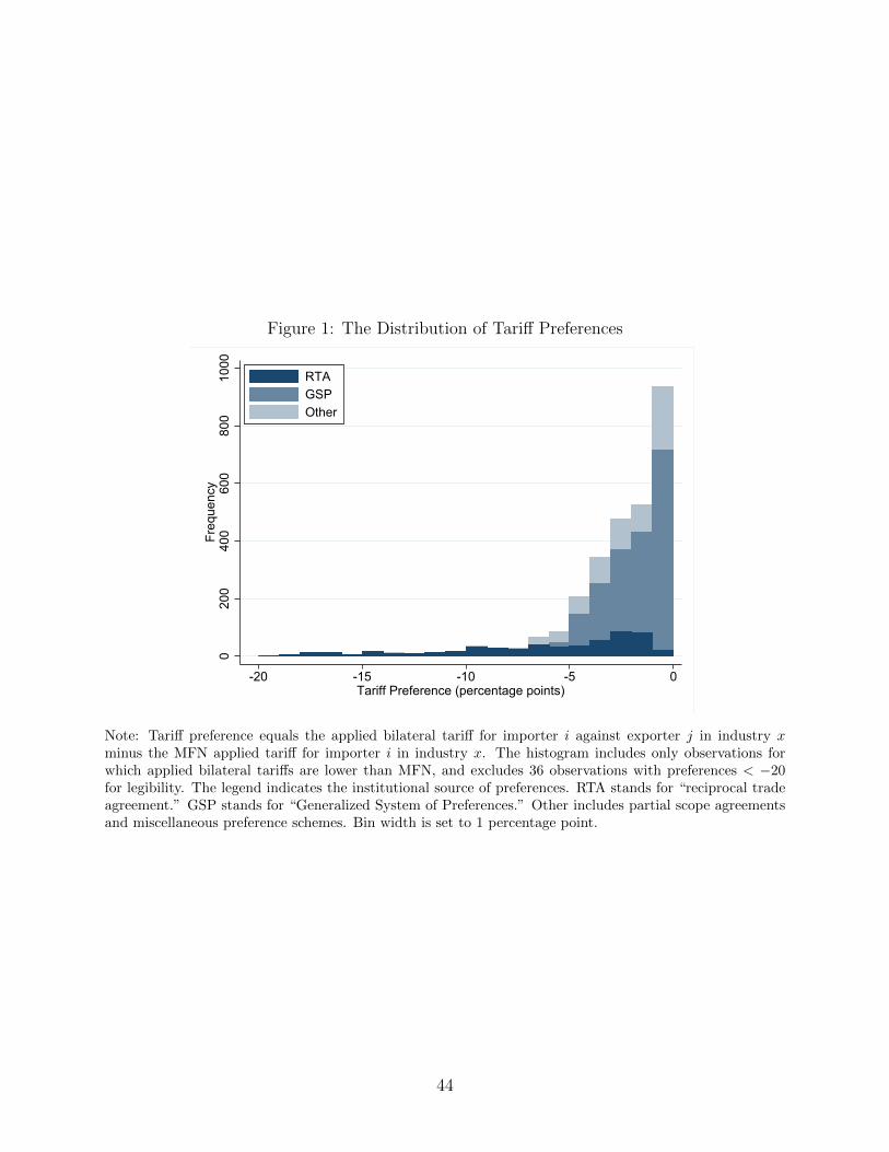
Figure 1: The Distribution of Tariff Preferences

020

040

060

080

010

00Fr

eque

ncy

-20 -15 -10 -5 0Tariff Preference (percentage points)

RTAGSPOther

Note: Tariff preference equals the applied bilateral tariff for importer i against exporter j in industry xminus the MFN applied tariff for importer i in industry x. The histogram includes only observations forwhich applied bilateral tariffs are lower than MFN, and excludes 36 observations with preferences < −20for legibility. The legend indicates the institutional source of preferences. RTA stands for “reciprocal tradeagreement.” GSP stands for “Generalized System of Preferences.” Other includes partial scope agreementsand miscellaneous preference schemes. Bin width is set to 1 percentage point.

44

Figure 2: Tariff Preferences and Domestic Value Added in Foreign Final Goods

BRA-AUS IDN-AUS IND-AUSMEX-AUSRUS-AUS TUR-AUSTWN-AUS

BRA-CAN IDN-CAN IND-CAN

MEX-CAN

RUS-CAN

TUR-CANTWN-CAN

BRA-EUNIDN-EUN IND-EUN

MEX-EUN

RUS-EUN

TUR-EUN

TWN-EUN

BRA-JPN IDN-JPNIND-JPN

MEX-JPN

RUS-JPN

TUR-JPN

TWN-JPNBRA-KOR IDN-KORIND-KOR

MEX-KORRUS-KOR TUR-KORTWN-KOR BRA-USAIDN-USA IND-USA

MEX-USA

RUS-USA TUR-USATWN-USA CHN-AUS

CHN-CAN

CHN-EUN

CHN-JPN

CHN-KORCHN-USA

-15

-10

-50

Tarif

f Pre

fere

nce

(per

cent

age

poin

ts)

2 4 6 8Log Domestic Value Added

(a) Textiles and Apparel

BRA-AUSIDN-AUS IND-AUSMEX-AUSRUS-AUS

TUR-AUS TWN-AUS

BRA-CANIDN-CAN IND-CAN

MEX-CAN

RUS-CAN

TUR-CAN TWN-CAN

BRA-EUNIDN-EUN IND-EUN

MEX-EUN

RUS-EUN

TUR-EUN

TWN-EUN

BRA-JPNIDN-JPNIND-JPN

MEX-JPN

RUS-JPN

TUR-JPN

TWN-JPNBRA-KORIDN-KORIND-KOR

MEX-KORRUS-KORTUR-KOR TWN-KOR

BRA-USAIDN-USA IND-USA

MEX-USA

RUS-USATUR-USA

TWN-USACHN-AUS

CHN-CAN

CHN-EUN

CHN-JPN

CHN-KORCHN-USA

-6-4

-20

Tarif

f Pre

fere

nce

(per

cent

age

poin

ts)

4 6 8 10Log Domestic Value Added

(b) All Manufacturing Industries

Note: Figure includes high-income importers and emerging economies exports in 2005. High-income countriesinclude Australia, Canada, the European Union, South Korea, and the United States. Emerging economiesinclude the other 9 countries listed in Table 1. Textiles and Apparel is WIOD sector 4, and All Manufacturingis WIOD sectors 4-16. Labels indicate exporter-importer pair.

45

A Theory Appendix

This appendix derives the optimal bilateral tariff when the quantities of value added usedin each sector and destination are endogenous. While we use a specific-factors structureto streamline the derivation of the optimal tariff in the main text, we show here that thepredictions we examine and the estimation framework we adopt are essentially the samein this more general setting. With the exception of those changes introduced below, allremaining assumptions are as in the main text.

In place of the specific-factors structure introduced in Section 1.2, we now assume thatproducers can adjust the quantity of value-added inputs used in production in response tovalue-added prices, subject to frictions. These frictions limit the substitutability of value-added inputs across end-use sectors or destinations, so that the equilibrium returns to valueadded may differ across countries and industries. Since the returns to value added depend inturn on final goods prices, the pattern of value added is a function of the complete vector ofworldwide final goods prices; i.e. ~ν ≡ ~ν(~r(~p;~ν)) ≡ ~ν(~p). Likewise, we collapse the argumentsfor the returns to value added in terms of worldwide final goods prices: ~r(~p;~ν(~p)) ≡ ~r(~p).

As before, national income is given by the sum of final goods production (measuredat local prices), tariff revenue, plus payments to domestic value added embodied in foreignproduction (DV A) and less payments to foreign value added used in local production (FV A):

I i = 1 + ~pi · ~qi(~p) +R(~p, I i) +∑s∈S

∑c 6=i∈C

rcsiνcsi︸ ︷︷ ︸

≡DV Ai(~p)

−∑s∈S

∑c 6=i∈C

riscνisc︸ ︷︷ ︸

≡FV Ai(~p)

. (A1)

There are two key differences relative to the baseline version of the model. First, there is asecond mechanism by which a tariff change affects the return to value added – in addition toaltering the prices of value added, ~r, changes in final goods prices can shift the equilibriumpattern of value added quantities used in production, ~ν. We will see these two effects asseparate elasticities on the DV A and FV A terms in the optimal tariff expression below.

Second, with endogenous value added, all elements of domestic local production, FV A,and DV A now depend on the complete vector of world prices via ~ν(~p). Commensurately,a change in any given bilateral tariff (on a particular good from a particular country) may(potentially) disrupt the entire world vector of prices in all sectors, in every country.54 Thesebroader price transmission relationships complicate exposition, but they do not fundamen-tally alter the key mechanisms in which we are most interested. There are simply morepotential indirect effects that operate through the endogenous reallocation of value addedacross other end-use sectors and ‘third’ countries (i.e. s 6= x ∈ S and c 6= i, j ∈ C.).

We assume, like before, that the government maximizes the weighted sum of nationalincome, consumer surplus, and individual producer influences. To simplify notation, wealso now assume that the political welfare weights are the same across trading partners and

54For intuition, consider a unilateral increase in τ ixj . In the baseline model in the text, this would cause

rjxi to fall, but νjxi would remain fixed by assumption. With endogenous value added, the reduction in rjxiwould cause value added to exit sector x in now-less-attractive country j, disrupting the worldwide patternof value added content quantities, ~ν, and thus the equilibrium pattern of worldwide final goods productionand prices.

46

sectors. The optimal tariff imposed by country i on a given final good x ∈ S imposed againstcountry j 6= i ∈ C is then given by:

τ ixj = arg max I i + ζ(~pi) + δi∑s

πis(~p)− δi∗FV Ai(~p) + δ∗iDV Ai(~p)]. (A2)

s.t. pix = τ ixjpjx and τ ixj ≤ τ i,MFN

x .

The first order condition of country i′s maximization problem is:

Gτ ixj= ∇I ·Dτ ixj

~p+∇ζ ·Dτ ixj~pi + δi

∑s

dπisdτ ixj

− δi∗dFV Ai

dτ ixj+ δ∗i

dDV Aidτ ixj

= 0. (A3)

In the first term, ∇I is the gradient of income with respect to the (1 × SC) world-pricevector, ~p, and Dτ ixj

~p is the (SC × 1) derivative of the world price vector with respect to

the bilateral tariff (so, ∇I · Dτ ixj~p = dI

dτ ixj). In the second term, the derivative of consumer

surplus, ∇V is the (1 × S) gradient vector of indirect utility with respect to each of the S

elements of the local price vector, ~pi, and Dτ ixj~pi is the (S × 1) derivative of the local price

vector with respect to the bilateral tariff. The last three terms are self-explanatory.Using Roy’s identity, collecting terms, and expanding the political economy and value

added terms yields:

Gτ ixj=

∑s

∑c6=i

[−M i

sc

dpcsdτ ixj

+ tiscpcs∇M i

sc ·Dτ ixj~p

]+

+δi~qi ·Dτ ixj~pi + (1 + δ∗i )∇DV Ai ·Dτ ixj

~p︸ ︷︷ ︸≡ dDV A

dτixj

−(1− δi∗)∇FV Ai ·Dτ ixj~p︸ ︷︷ ︸

≡ dFV Adτxj

= 0. (A4)

Above we use∇M isc to represent the gradient of bilateral imports of each good s from trading

partner c to country i with respect to the complete world price vector, and ∇DV Ai and∇FV Ai to represent respectively the gradients of country i’s domestic value added embodiedin foreign production, and foreign value added returns used in country i’s production (againwith respect to the world price vector).

Paralleling our earlier approach, we introduce the term ΩRixj to capture the (potential)

effects on trade revenue collected on exports other than those in sector x from country j.55

Dividing through by the bilateral trade volume and dpjxdτ ixj

yields the optimal tariff expression:

tixj εixj = 1−

δi~qi · ~Λiixj

M ixj

− (1 + δ∗i )∇DV Ai · ~Λixj

M ixj

+ (1− δi∗)∇FV Ai · ~Λixj

M ixj

− ΩRixj , (A5)

where εixj is the general equilibrium analog to the bilateral export supply elasticity in the

55ΩRixj ≡∑s

∑c6=i,j

[−Eisc

dpcsdτ i

xj+ tiscp

cs∇~pEisc ·Dτ i

xj~p

]+∑s6=x

[−Eisj

dpjsdτ i

xj+ tisjp

js∇~pEisj ·Dτ i

xj~p

].

47

baseline version of the model and ~Λixj ≡ Dτ ~p

dpjx/dτixj

is the (SC×1) vector of the induced changes

in the world price vector following a change in τ ixj, relative to the price change in the directly-

affected sector x in country j.56 Similarly, ~Λiixj ≡

Dτ ~pi

dpjx/dτixj

is the (S × 1) vector of induced

changes in the local (country i) prices relative to the change in pjx. Let ΩRixj ≡ ΩRi

xj/(dpjxdτ ixj

M ixj)

again capture the tariff revenue effects of trade diversion in outside sectors and countries viachanges in world price and the pattern of value added use.

Apart from the more complex general equilibrium price mappings, the basic form ofthe optimal tariff expression in (A5) is unchanged from the main text. As before, we candecompose the two value added terms into elasticities and empirically-measurable quantitiesof DV A and FV A. In the process, we also separate out the “direct” effect of the bilateraltariff change on the price of the target-good x in trading partners i and j apart from otherindirect “general equilibrium” effects.

∇DV Ai · ~Λixj

M ixj

=1

M ixj

∑s

∑c 6=i

(νcsi∇rcsi + rcsi∇νcsi) · ~Λixj

=∑s

∑c 6=i

(rcsiν

csi

pcsMixj

)(pjxrcsi∇rcsi · Λixj︸ ︷︷ ︸≡εrc

si(ijx)

+pjxνcsi∇νcsi · Λixj︸ ︷︷ ︸≡ενc

si(ijx)

)

=rjxiν

jxi

pjxM ixj

(εrjxi + ενjxi )︸ ︷︷ ︸direct effect

+∑c 6=i

∑s 6=x

rcsiνcsi

pjxM ixj

(εrcsi + ενcsi ) +∑c6=i,j

rcxiνcxi

pjxM ixj

(εrcxi + ενcxi)︸ ︷︷ ︸indirect (GE) effects ≡ΩDVAixj

= (εrjxi + ενjxi )DV AjxipjxM i

xj

+ ΩDV Aixj (A6)

56Formally, εixj ≡pjxEi

xi

1

∇~pEjxi·~Λixj

is the bilateral export supply elasticity allowing the tariff change to work

through the complete vector of final good prices (in addition to the foreign local price, pjx as is standard).

Note that the elements of the ~Λ vector, which take the form ofdpcsdτ /

dpjxdτ , are the inverse of the λ(≡ dpj

dτ /dpcsdτ )

terms used in the main text (and in Bagwell and Staiger (1999)). We make this change both for notational

convenience and because standard modeling assumptions render most elements of the numerator of our ~Λvector zero (consistent with the absence of general equilibrium effects of a bilateral tariff change).

48

Following the same procedure for the FV A term:

∇FV Ai · ~Λixj

M ixj

=∑s

∑c 6=i

(riscν

isc

pjxM ixj

)(pjxrisc∇risc · Λixj︸ ︷︷ ︸≡εri

sc(ijx)

+pjxνisc∇νisc · Λixj︸ ︷︷ ︸≡ενi

sc(ijx)

)

=∑c 6=i

rixcνixc

pjxM ixj

(εrixc + ενixc)︸ ︷︷ ︸direct effect

+∑c 6=i

∑s6=x

riscνisc

pjxM ixj

(εrisc + ενisc)︸ ︷︷ ︸indirect effects ≡ΩFV Aixj

= (εrix∗ + ενix∗)FV AixpixM

ixj

+ ΩFV Aixj . (A7)

Finally, we also separate the political economy term into direct (sector x) and indirect(sectors s 6= x ∈ S) components:

δi~qi · ~Λiixj

M ixj

= − δiqix|λixj|M i

xj︸ ︷︷ ︸direct effect

+∑s 6=x

δiqisλisjM

ixj︸ ︷︷ ︸

indirect effect≡ΩPEixj

, (A8)

where λixj ≡dpjxdτ ixj

/ dpix

dτ ixj< 0, as in the main text.57

Substituting the decompositions in (A6)-(A8) into the optimal tariff expression, we canrewrite the optimal bilateral tariff expression:

tixj =1

εixj

(1+

δiqix|λixj|M i

xj︸ ︷︷ ︸(+)

−(1+δ∗xi)(εrjxi + ενjxi )

DV AjxipjxM i

xj︸ ︷︷ ︸(−)

+ (1−δix∗)(εrix∗ + ενix∗)FV AixpixM

ixj︸ ︷︷ ︸

(−) iff δix∗<1

−Ωixj

), (A9)

where Ωixj captures all of the “indirect” effects of the tariff change on via country i’s tariff

revenue, domestic political economy and FV A in sectors other than x, as well as the DV Ainfluences other sectors and in the returns to DV A in trading partners other than j.58

This optimal tariff expression is the general equilibrium analog to the specific factorsversion of the model presented in the main text.59 Focusing on the direct bilateral, sector-xelements, we see that the optimal tariff is (again) inversely related to the bilateral tradeelasticity, augmented by domestic political economy, DV A, and FV A motivations. The keydifference is that the quantitative effects of DV A and FV A on the optimal tariff dependon the elasticity of both value added prices (via εr) and quantities (via εν) with respectto tariff-induced price changes. Empirically, these two elasticities will be captured by ourcoefficient estimates, together with the political economy weights.

57Similarly, define λisj ≡dpjsdτ i

xj/dpisdτ i

xj∀s ∈ S; the sign of λisj is ambiguous for s 6= x.

58 Ωixj ≡ ΩRixj − ΩFV Aixj + ΩDVAixj + ΩPEixj .59Most of the “nuisance” general equilibrium effects would arise in a broad class of GE frameworks, and

are not about value-added components of trade, per se.

49

B Data Appendix

B.1 Computing Value Added Content

As noted in the text, our measures of domestic content in foreign production and foreigncontent in domestic production can be motivated as an application of the ‘global value chain’decomposition of final goods developed in Los, Timmer and de Vries (2015).60 We brieflydescribe the computation here.

As in the main text, let i, j ∈ 1, 2, . . . , C denote countries and s ∈ 1, 2, . . . , S denoteindustries. The World Input-Output Database includes an input shipments matrix, IIt, with(S × S) dimensional block elements IIijt(s, s

′) that record input shipments from sector s incountry i to sector s′ in country j. These matrices can easily be re-written in share form.Let Aijt be a (S×S) dimensional matrix with elements Aijt(s, s

′) = IIijt(s, s′)/Yj(s

′), whichrecord the share of inputs from sector s in country i used by sector s′ in country j as ashare of gross output in sector s′ in country j. Then assemble blocks Aijt into the globalinput-output matrix At. The Leontief inverse of the global input-output matrix, [I −At]−1,times any (SC × 1) vector of final goods output equals yields the (SC × 1) vector of grossoutput (from all countries and industries) required to produce those final goods.

Let fit be the (S × 1) vector of final goods produced in country i, which are directlyreported in the World Input-Output Database. Stack these into a (SC × 1) vector ft,and compute Yt ≡ [I − At]−1diag(ft). Breaking this down, Yt contains block elements Yijtwhich are S × S matrices describing output from country i used (directly or indirectly) toproduce final goods in country j. Each sub-component Yijt(s, s

′) is the amount of outputfrom industry s in country i used in producing final output in industry s′ in country j.

These output requirements can be translated into value-added content requirements ifwe know the value added to output ratios in each sector s and source country i: Rit(s).The total amount of value added from country i embodied in country j’s production in aparticular industry x ∈ S is: V Ajxit ≡

∑sRit(s)Yijt(s, x). We use these value added elements

to construct proxies for country i’s domestic value added embodied in foreign productionof each sector s ∈ S in trading partner j 6= i ∈ C (DV Ajsit) and foreign value addedembodied in country i’s domestic production of s (FV Aist). Specifically, for a given good x,DV Ajxit ≡ V Ajxit and FV Aixt ≡

∑c 6=i∈C V A

ixct.

We compute value added content using the disaggregated 40 country version of the WIODdata set. We then aggregate value-added content across EU countries to form the EUcomposite, because EU countries have common external tariffs and trade policy.

60The global value chain traces backward through the production chain from final goods to identify thesources of value added in those goods. This is different than the value-added export decomposition developedby Johnson and Noguera (2012), which traces value added forward through the production chain to determinewhere value added from each country is ultimately consumed. It is also different than the decomposition ofgross exports advanced by Koopman, Wang and Wei (2014).

50

B.2 Tariffs

B.2.1 Data Details

As noted in Section 3.2, we draw our data from UNCTAD (TRAINS) and the WTO via theWITS website. We faced a number of challenges in transforming these raw data sources intoa consistent set of tariff measures. Below we describe our procedure to clean and aggregatethe tariff data.

First, there are a handful of instances in which a country’s entire bilateral tariff scheduleis missing in one of our four benchmark years. In most of these cases, when we can beconfident that there were no major trade policy changes in that year, we take the tariffschedule from the closest available year for that country. In a few instances, we insteadexclude the importer in that particular year. The following importing countries and yearsare excluded on these grounds: China (1995, 2000), South Korea (1995, 2000), Taiwan (1995,2000), and Russia (2000). These countries are included as exporters in all years.

Second, there are cases where tariffs are misreported, or entirely missing, for a subset ofproducts or partners in a given year. In some instances, we are able to resolve these idiosyn-cratic problems through inspection. For example, a country’s data may omit a particulartariff preference program in a given year, even though that program exists in the country’sdata in the years immediately before and after the missing year. While it is possible thatthese programs were temporarily suspended, our investigative efforts to validate such pos-sible temporary suspensions typically uncovered no corroborating evidence consistent witha genuine change in policy. Therefore, we use information on preferences from surroundingyears. In a handful of other cases in which we cannot resolve these problems, we insteadrecord tariffs as missing.

Third, tariff lines (products) are not defined consistently across countries at the mostdisaggregated (HS-8+) level. Therefore, we take the unweighted mean across (HS-8+) tarifflines within each HS 6-digit Harmonized System category, which are standardized acrosscountries. We then classify these HS 6-digit categories into final versus intermediate useusing BEC classifications as described in the text.

Fourth, some HS 6-digit tariff lines have multiple preferences recorded in the data. Forexample, Canada may report two tariffs for imports from Mexico: one under NAFTA andanother under GSP. When one of the reported tariffs derives from an Article XXIV freetrade agreement or customs union, we treat that tariff as the applicable tariff. When two ormore non-FTA/CU tariffs are present, we adopt the lower of the two rates as the applicabletariff. In the end, we have information on the preference scheme under which every bilateralpreferential tariff is offered in the data.61

Fifth, there are several technical issues that need to be addressed pertaining to exit/entryof HS 6-digit codes in the data (either over time or across countries at a given point in time)and non-ad valorem tariffs. We start with a data set that includes all available HS 6-digittariffs. We then refine the data in two dimensions. First, we discard all HS 6-digit sectors(by importer) in which tariffs are applied exclusively as specific duties.62 Second, we retain

61One hurdle to identifying preference programs is that program identifiers in the raw UNCTAD/TRAINSdata are often difficult to parse. When necessary, we cross-reference various secondary sources to identifythe relevant preference schemes.

62To clarify, some importers may apply ad valorem tariffs in a given HS 6-digit sector, while others apply

51

only HS 6-digit categories for which we have a fully-balanced panel of tariffs — as in, foreach importer, a given HS 6-digit tariff is observed for all partners in all years. This allowsus to construct consistent tariff averages over time, as well as across partners at a given pointin time.63

We aggregate these HS 6-digit tariffs to the WIOD industry level using simple aver-ages, which yields measures for applied bilateral and MFN tariffs at the importer-exporter-industry-year level. We define a bilateral country pair to have a preferential tariff in agiven industry and year if any bilateral applied HS 6-digit tariff for that importer-exporter-industry-year cell is below the MFN applied rate. Typically, the preference scheme in eachcell is unique, and so we record the relevant program as the source of the tariff preferences atthe industry level. For a small handful of cells, there are multiple preference schemes activewithin a given bilateral-industry-year cell (some HS 6-digit tariff lines within the industryreceive preferences under one program, while others receive preferences under a differentprogram). In these cases, we record the more important preference program, which typicallyaccounts for the vast majority of preferences in the industry.

B.2.2 Sources of Tariff Preferences

As noted in the text, there are preferential tariffs in about a third of the importer-exporter-industry-year cells. The GSP program accounts for the majority (69 percent) of these pref-erences. In our data, there are three primary sources of time-varying discretion in the GSPprogram. The first is that each GSP granting country chooses the set of countries to which togrant GSP access. The second is that each GSP granting country chooses the set of industriescovered by GSP, where industry exemptions apply to all GSP-partners. The third is thatthe importing country chooses the level of the GSP tariff to apply to its GSP-partners.64

Each of these decisions is updated over time, as countries introduce or renew their GSPprograms.65 One important point is that the way GSP is recorded in our data understatesthe actual degree of discretion with which the GSP program is applied in practice.66 As

specific duties in that sector. We only discard the HS sector for importers that actually apply specific duties,and retain the sector for other importers. Specific duties account for less than 2 percent of the HS 6-digit tarifflines for final goods. Discarding them avoids the well-understood concerns involved in converting specifictariffs to ad valorem equivalents, which are particularly problematic for aggregation or comparability acrossindustries and countries.

63The cost of discarding unbalanced observations is that we lose about 13 percent of the (non-specificduty) importer-exporter-HS6-year tariff observations. We have confirmed that average bilateral industry-level tariffs computed from this balanced data are comparable to unbalanced averages that use all of the data.Further, tariff preferences (applied minus MFN tariffs) are nearly identical in balanced and unbalanced HS6-digit tariff panels. Therefore, while this balancing step is useful for internal consistency, it is not importantfor the results.

64Regarding the second and third items, GSP preferences are reported at the HS 6-digit level in ourdata. As we aggregate, we take the simple average of GSP and MFN tariffs within each WIOD industry.Consequently, composite industry-level tariffs reflect both the set of HS 6-digit categories that receive tariffpreferences as well as the size of those tariff preferences. In our data, GSP tariffs do not vary across the set ofpartners included in each importer’s GSP program (with a few minor exceptions). In some industries, no HS6-digit category receives preferences, in which case the entire industry is excluded from the GSP program.

65GSP preferences are identified by the “year” of the importer’s GSP program in the raw tariff data.66Specifically, importers deviate from the published GSP tariff schedule in our data for various (largely

discretionary) reasons. For example, Blanchard and Hakobyan (2014) review the vagaries of country-product

52

such, our results regarding discriminatory preferential tariffs in the GSP program are likelyconservative, since our data understates the true extent of discretion under GSP.

Bilateral trade agreements and other miscellaneous preference programs make up theremainder of preferences in our data. The miscellaneous preferences are difficult to classifyconcisely. For example, one of the largest miscellaneous preference programs we observeis the so-called “Australia Tariff” in Canada’s tariff schedule, under which Canada affordsAustralia preferential treatment for roughly 300 HS 6-digit categories.67 Other idiosyncraticpreference schemes are more limited, sometimes covering only a few miscellaneous HS 6-digittariff lines.

Turning to bilateral trade agreements, we classify these preferences programs into twogroups, consistent with our theoretical discussion in Section 1.4: potentially reciprocal tradeagreements (RTAs) and non-reciprocal trade agreements.68 Our baseline approach to classi-fying these agreements is as follows.

We define country i to have a potentially reciprocal trade agreement (RTA) with country jin year t if those countries have a trade agreement in force that was notified to the WTO underArticle XXIV.69 In the language of Article XXIV, these are commonly referred to as CustomsUnions and Free Trade Areas. Article XXIV is a useful device to classify agreements becauseit requires countries to eliminate tariffs/duties on ‘substantially all trade’. This requirementis evident in practice, as these agreements have much broader coverage on average than othertrade agreements. Nonetheless, we repeat two points here that we emphasized in the maintext. The first is that Article XXIV agreements still contain carve outs, which leave positivetariffs in many industries. The second is that some agreements in force have long, oftenhighly asymmetric phase-in schedules.70 These phase-in schedules are a source of discretioneven inside reciprocal agreements. As a result of both of these sources of discretion, wetreat these Article XXIV agreements as potentially reciprocal and test for the implicationsof reciprocity (i.e., that DVA should not influence tariffs inside RTAs).

We classify remaining trade agreements as non-reciprocal. These agreements are exclu-sively struck between developing countries, and most are notified to the WTO under theEnabling Clause.71 Because they are notified under the Enabling Clause, these agreements

exclusions in the United States GSP program, including the discretionary application of “competitive needslimitations” and revocation of GSP privileges for violations of intellectual property and worker rights.

67Though a legacy of British colonial tariff preferences, this program was amended and re-authorizedduring our sample period, in 1998.

68A subtle note is that our language here differs a bit from the way the WTO describes these agreements.The WTO refers to all WTO-notified agreements as ‘reciprocal’ in that they involve the exchange of tariffpreferences. We take ‘reciprocal’ to mean a sufficiently comprehensive and symmetric exchange of tariffpreferences that nullifies bilateral terms-of-trade externalities within the agreement. There is not a strongpresumption that terms-of-trade externalities are neutralized by partial agreements, covering a minority oftrade. Whether agreements do achieve terms-of-trade neutralization is fundamentally an empirical question,which we address via our testing procedure.

69This definition identifies a set of reciprocal agreements among countries in our data that correspondsexactly to the set of FTAs and Customs Unions identified by Baier and Bergstrand (2007).

70A nice feature of our data is that we observe this phase-in process. For example, for the US-Australiafree trade agreement, the United States implemented preferences immediately when the agreement enteredinto force, whereas Australia’s implementation of preferences was more gradual. Similar issues arise for otheragreements adopted within in our sample period (e.g., EU-Mexico, Japan-Mexico, etc.).

71One important agreement — a preferential agreement between Mexico and Brazil — has not been

53

are not bound by the ‘substantially all trade’ requirement of Article XXIV agreement. Thedata confirm that these agreements are much narrower in scope, having typical HS 6-digitcoverage rates of less than 20 percent, compared to over 90 percent for RTAs. Reflectingthis different standard, two of these agreements (the Asia-Pacific Trade Agreement and theGlobal System of Trade Preferences) are commonly referred to as “partial scope” agreements.

Table B1 lists the trade agreements in our data and our classification of them into re-ciprocal vs. non-reciprocal agreements. Because the division of agreements into reciprocalvs. non-reciprocal agreements is a subjective one, we also present an alternative broaderclassification in the table. Our broad RTA definition includes all Article XXIV agreementsplus additional comprehensive agreements between developing countries. It is worth notingthat these agreements are not necessarily free trade agreements, as commonly understood.For example, for the Brazil-Mexico agreement, the median tariff is 13 percent (the minimumis roughly 5.5 percent) at the industry level. While we focus on the definition of RTAs asWTO-notified Article XXIV agreements in our main results, we present supplemental resultsfor the broad RTA classifications in Appendix C.

B.2.3 Another Look at MFN as a Constraint on Bilateral Applied Tariffs

An additional salient feature of the data is that tariff preferences are constrained by the MFNrule. When the MFN tariff is low, so too is the potential scope for tariff preferences, sincetariffs are then bound between zero and the MFN rate. Given this, we would expect thatboth the absolute value of the mean preference and the standard deviation of preferenceswould be low when average MFN rates are also low. In Panel (a) of Figure B1, we seethat preferences are indeed near zero when MFN tariffs are low (note the y-axis recordsnegative values, since we define preferences as bilateral applied tariffs minus MFN tariffs).In Panel (b), we see that variability in preferences is rising with mean MFN tariffs. Boththese patterns are consistent with MFN-censoring constraining variation in the data.

notified to the WTO, according to the WTO’s trade agreement database [http://rtais.wto.org/UI/PublicMaintainRTAHome.aspx].

54

Table B1: Classifying Trade Agreements

Years in Force WTO Notification RTA Broad RTA

Bilateral AgreementsAustralia-United States 2005, 2009 Article XXIV yes yesBrazil-Mexico 2005, 2009 None no yesChina-Indonesia (ASEAN) 2005, 2009 Enabling Clause no yesEuropean Union-Mexico 2000, 2005, 2009 Article XXIV yes yesEuropean Union-Turkey 2000, 2005, 2009 Article XXIV yes yesIndonesia-South Korea 2009 Article XXIV yes yesJapan-Indonesia 2009 Article XXIV yes yesJapan-Mexico 2005, 2009 Article XXIV yes yes

Regional AgreementsAsia-Pacific Trade Agreement 2005, 2009 Enabling Clause no noGlobal System of Trade Preferences 1995, 2000, 2005, 2009 Enabling Clause no noNorth American Free Trade Agreement 1995, 2000, 2005, 2009 Article XXIV yes yes

Note: Asia-Pacific Trade Agreement includes China, India, and South Korea (among others). Global Systemof Trade Preferences includes Brazil, India, Indonesia, Mexico, and South Korea (among others). The NorthAmerican Free Trade Agreement (NAFTA) includes Canada, Mexico, and the United States.

Figure B1: Mean and Standard Deviation of Tariff Preferences versus MFN Tariffs, by Sector

1

3

45

6

7

9

10

11

12

13

14

15

16

-1.4

-1.2

-1-.8

-.6-.4

Mea

n

5 10 15 20Mean MFN Applied Tariff

(a) Mean of Tariff Preferences

13

4

5

6

7

9

10

11

12

13

14

1516

1.5

22.

53

3.5

4S

tand

ard

Dev

iatio

n

5 10 15 20Mean MFN Applied Tariff

(b) Standard Deviation of Tariff Preferences

Note: Tariff preference equals the applied bilateral tariff for importer i against exporter j in industry x minusthe MFN applied tariff for importer i in industry x. Both means and standard deviations are computed bysector, pooling all importer-exporter-year observations within sector, including those with zero preferences.The markers denote WIOD sector numbers, included in Table 1.

55

C Supplemental Results

This appendix provides supplemental results. Section C.1 presents robustness checks relatedto estimation of Equation (16). Section C.2 presents instrumental variables estimates ofEquation (19).

C.1 Robustness Checks for Domestic Value Added

In this section, we perform two checks on our baseline estimates.First, we demonstrate that our main results regarding the role of domestic value added

are robust to how we define reciprocal trade agreements. To so so, we replicate results fromTables 2 and 3 using a broader definition of RTAs. This broader definition, introducedin Appendix B [Section B.2.2 and Table B1], includes bilateral agreements adopted underArticle XXIV plus comprehensive agreements not arising under Article XXIV.

In columns (1)-(3) of Table C1, we repeat the inside versus outside RTA analysis fromTable 2. As before, the negative influence of DVA on tariffs manifests itself exclusivelyoutside RTAs. Further, in columns (4) and (5), we show that the point estimate on DVA isnegative in this alternative no-RTA sample, comparable in size to the main point estimates.We conclude that the exact definition of RTAs has little bearing on our analysis. Nonetheless,we retain non-Article XXIV agreements in our baseline no-RTA sample throughout the paper,because adoption of these is itself a manifestation of discretionary trade policy.

Second, we show that our baseline DVA results are robust to adding bilateral controls toproxy for potential omitted confounding variables. The first control we add is log bilateralfinal goods imports. In column (2) of Table C2, the coefficient on exports is significant,but the point estimate on log DVA is unchanged relative to the baseline. This implies thatimports are essentially orthogonal to log DVA, given the controls. This is sensible, sincewe have already removed a substantial component of import variation by interacting importdecile indicators with the importer-industry-year fixed effects.

The second set of controls are measures of bilateral characteristics (often used as prox-ies for trade costs in the gravity literature), including distance, colonial linkages, commonlanguage, and contiguity (common border).72 We do this to rule out that omitted variables(either the proxies themselves, or variables that are correlated with the proxies) spuriouslydrive our results.

In Table C2, columns (3)-(6) report OLS estimates and columns (7)-(10) report IV es-timates with DVA-in-Services as the instrument. As is evident, the coefficient on log DVAremains negative and significant after adding these controls, while the proxy variables them-selves are almost never significant.

72We obtain these variables from the CEPII GeoDistance Database: http://www.cepii.org/CEPII/fr/

bdd_modele/presentation.asp?id=6. One complication is that these characteristics pertain to individualbilateral country pairs, but we have a composite non-country entity (the EU) in our data. We thereforedefine bilateral characteristics vis-a-vis the EU by taking GDP-weighted averages of bilateral characteristicsdefined for each individual EU country. This implies that colonial linkages, common language, and contiguityare not strict indicator variables, as their weighted averages can lie between zero and one when the EU is atrading partner.

56

One point of interpretation is worth emphasizing here. The gravity variables could influ-ence DVA in two ways. First, they could have a direct effect, either because they influencetariffs for various unmodeled reasons, or because they proxy for omitted determinants oftariffs. Second, they could have an indirect effect, via DVA. That is, DV Ajxi is high when isupplies inputs to j, and input sourcing is naturally correlated with trade costs. The reasonto point this out is that this likely explains why the DVA falls slightly when we add thesecontrols. By adding them, we are mechanically removing some of the meaningful variation inDVA that drives tariffs and therefore diminishing its direct effect. Given this interpretationconcern, as well as the insignificant point estimates on the proxies, we omit them in theremaining analysis in the main text.

C.2 Identifying the Influence of Foreign Value Added via Instru-mental Variables

In Table 5, we presented OLS estimates of Equation (19), with two alternative sets of fixedeffects. We noted that while one might be concerned about the endogeneity of foreignvalue added with respect to tariffs, this should bias the coefficient upward (i.e., towardzero/positive values, given that the point estimate is negative). In this sense, the OLSestimate of the FVA effect may be conservative. Further, we noted there that IV estimatesin that specification tend to support this interpretation. We present the details of thatargument here.

To instrument Equation (19), we require instruments for DV Ajxit, FV Aixt, FG

ixt, and

IM ixjt. Needless to say, finding four instruments is a formidable challenge.73 For DV Ajxit,

we use the DVA-in-Services instrument presented previously in Section 4.1. We constructthree additional instruments for FV Aixt, FG

ixt, and IM i

xjt as follows.

Instrument for FG The instrument for final goods production is based on predictingfinal goods production for industry x in country i by taking a weighted average of total finalexpenditure in destinations j to which i sold output in a base period. Let FGi

xjt be the valueof final goods shipments from country i to j in industry x at date t. Letting 0 denote a baseperiod, then total final goods production at date t can be written as:

FGixt = FGi

x0

∑j

(FGi

xj0

FGix0

)[FGi

xjt

FGixj0

FGxj0

FGxjt

](FGxjt

FGxj0

), (C1)

where FGxjt is total final expenditure on industry x in destination j. The first term recordsthe shares of final goods production sold to each destination in the base period. The middleterm in square brackets records changes in final goods expenditure shares. The third termrecords changes in final expenditure levels. For the purposes of constructing an instrument,

73This particularly challenging in our context for two reasons. First, the fixed effects structure we adoptrules out many possible country, industry, or even country-industry instruments. Second, the potentially en-dogenous explanatory variables are correlated among themselves for structural reasons (e.g., FV Aixt dependson the level of FGixt), and so many instruments for them are also correlated among themselves. As a result,many potential instruments suffer from weak instrument problems. We explicitly address weak instrumentconcerns below.

57

suppose that final goods import shares are constant over time, so thatFGixjtFGixj0

FGxj0FGxjt

= 1. And

then re-write the expression in logs:

ln(FGi

xt

)≈ ln

(FGi

x0

)+ ln

(∑j

(FGi

xj0

FGix0

)FGxjt

FGxj0

). (C2)

Because we include importer-industry fixed effects in all specifications, final goods pro-duction in the base year (ln (FGi

x0)) is redundant. For identification, we rely solely on timevariation in final goods production at the importer-industry level (with importer-specific andindustry-specific effects differenced out), for which the second term is an instrument. Putdifferently, what we actually need is an instrument for growth in final goods production,and our instrument aggregates growth rates in destination expenditure using weights thatdepend on sales shares in the benchmark year. In constructing the instrument, we treat 1995as the benchmark year.

Instrument for FVA The instrument for foreign value added in domestic productionbased on predicting how much foreign value added in used by industry x in country i usinginformation on the foreign supply of value added in upstream industries. Intuitively, if foreignsupply capacity grows quickly, then we expect the amount of foreign value added used indomestic production to rise. To capture this idea, we build an instrument as follows.

Let FV Aijt(s, x) be the value added from country j and industry s used by industry xcountry i in production of final goods at date t. Again letting 0 denote a base period, FV Aixtcan be written as:

FV Aixt = FV Aix0

∑j 6=i

∑s

[(FV Aijt(s, x)

FV Aix0

)(FV Aijt(s, x)

FV Aij0(s, x)

V Ajs0V Ajst

)(V Ajst

V Ajs0

)], (C3)

where V Ajst is total value added added in sector s of country j at date t. Similar to above,

suppose that the value-added export shares are constant over time, soFV Aijt(s,x)

FV Aij0(s,x)

V Ajs0V Ajst

= 1,

and re-write the expression in logs:

ln(FV Aixt

)≈ ln

(FV Aix0

)+ ln

(∑j 6=i

∑s

(FV Aijt(s, x)

FV Aix0

)V Ajst

V Ajs0

). (C4)

As above, the base year level of foreign value added (ln (FV Aix0)) will be absorbed by ourfixed effects. The second term is then an instrument for growth in foreign value added used indomestic production over time. We again treat 1995 as the benchmark year in constructingthe instrument.

Instrument for Final Goods Imports To instrument for final goods imports, we mea-sure bilateral final goods imports at the industry level in 1970, prior to the introduction ofthe tariff preferences observed in our data. We use bilateral trade data at the SITC 4-digit(Rev. 2) level from the NBER-United Nations Trade Data [Feenstra et al. (2005)]. We

58

extract SITC categories corresponding to final goods using the BEC classification, and thenconcord SITC categories to our WIOD industries via ISIC industries.74

Estimation and Results Using these instruments, we re-estimate the linear specificationsin Table 5 and present the results in Table C3, along with the baseline OLS estimates fromTable 5 for reference. In Columns (1) and (3), we instrument for the three ratios on the righthand side of Equation 19 by constructing the ratio of the instruments for the numerator ineach ratio to the instrument for final goods imports.75 In columns (2) and (4), we do thesame for DVA and instrument for final goods imports to identify γIP + γFV A.

In Panel A, IV estimates are negative for domestic value added, negative for foreignvalue added, and positive for final goods production. These are consistent with the OLSsign estimates. In terms of magnitudes, the IV point estimates tend to move away fromzero relative to OLS. That said, the 2SLS point estimates are substantially less precise thanOLS. Nonetheless, one can reject the null that the import penetration and FVA ratios areexogenous in a Durbin-Wu-Hausman endogeneity test.76

In Panel B, we replicate the IV estimates for the sample excluding RTAs. The IVestimates here also broadly confirm the OLS estimates, though the details are more nuanced.The point estimate on DVA doesn’t move between the OLS and IV estimates, but becomesinsignificantly different than zero in the IV estimation due to the loss of precision. We cannotreject that DVA is exogenous in a Durbin-Wu-Hausman endogeneity test. Given our priorresults concerning the role of DVA – both in Panel A and in previous IV-specifications, we seeno reason to change our views on the sign of the DVA effect based on these results. Turningto FVA, the coefficient on FVA becomes negative and significant when we instrument here.This brings the FVA results in this sub-sample more in line with the full sample, includingRTAs. Further, we can easily reject exogeneity of the FVA-Ratio here.

Together with our previous IV results, these results corroborate our interpretation of theOLS estimates as indicative of causal relationships. In particular, the new concern in thisspecification concerns the role of FVA. Recalling that the principal endogeneity concern isthat tariffs raise FVA and thus bias the the FVA coefficient upward (toward zero/positivevalues), we argued in the text that our OLS estimates likely understate FVA effects. The IVresults are broadly consistent with this interpretation. That said, we are reluctant to takethe magnitude of the FVA estimate too seriously here due to the wide confidence interval.

One final point to note is that we report two-stage least squares standard errors (clusteredby importer-exporter pair) in the table. The appropriateness 2SLS standard errors is notobvious: the high correlations among endogenous variables and therefore the instrumentswe use for them could give rise to weak instrument problems. Therefore, in the table, wereport various weak-IV statistics to gauge the reasonableness of the 2SLS standard errors.

74Because country definitions have changed over time, we concord historical countries to modern entitiesas best we can. For example, Germany today corresponds most closely to the former Federal Republic ofGermany. Russia today corresponds to the former USSR. And so on. Further, more trade flows in theNBER-UN data are zero in 1970 than are zero today, likely due both to true changes from zeros to positivevalues over time and differences in reporting thresholds and/or missing data in the two data sources. Inorder to use the whole sample, we replace zeros in 1970 with the smallest values observed in the data.

75Including the instruments separately, without imposing this ratio restriction, yields similar results.76Testing the exogeneity of the DVA-Ratio alone, one cannot reject exogeneity.

59

We report statistics that allow for clustering – including tests for under-identification andweak identification [Kleinbergen and Paap (2006)] and conditional first-stage F statistics[Sanderson and Windmeijer (2015)]. These statistics suggest that that 2SLS standard errorsare acceptable.77 Nonetheless, we also computed Anderson-Rubin style confidence intervalsthat are robust to weak identification. These are comparable to the 2SLS confidence intervalsand do not alter inference in any important way.

77In interpreting these statistics, an unfortunate fact is that there is little guidance about what the valuesof these cluster-robust statistics need to be to be on safe ground. Values of 10 or above for the conditional Fstatistics are typically thought to be safe. The rK statistics compare reasonably favorably to critical valuesdeveloped for homoskedastic models.

60

Table C1: Bilateral Tariffs and Domestic Value Added in Foreign Production with BroadDefinition of RTAs

No RTAFull Sample No RTA Linear IV

(1) (2) (3) (4) (5)

Log DVA: ln(DV Ajxit) -0.43** -0.11* -0.14***(0.17) (0.062) (0.049)

Log DVA Outside RTAs: [1−RTAijt]×ln(DV Ajxit) -0.49** -0.50*(0.20) (0.29)

Log DVA Inside RTAs: RTAijt×ln(DV Ajxit) 0.030(0.30)

Reciprocal Trade Agreement: RTAijt -3.73*** -6.26** -6.17***(0.65) (2.47) (1.76)

Observations 8,853 8,853 8,853 8,076 8,076R-Squared 0.991 0.991 0.991 0.998 0.998

Note: Dependent variable in all columns is the applied bilateral tariff of country i in industry x againstexporter j at time t: tixjt. Log DVA (ln(DV Ajijt)) is domestic value added from the importing country(i)embodied in final production in industry x in the exporting country (j). Reciprocal Trade Agreement isan indicator that takes the value one if i and j have a reciprocal trade agreement in force, according tothe broad definition in Table B1. Standard errors (in parentheses) are clustered by importer-exporter pair.Significance levels: * p < .1 , ** p < .05, *** p < .01.

61

Tab

leC

2:B

ilat

eral

Tar

iffs

and

Dom

esti

cV

alue

Added

inF

orei

gnP

roduct

ion

wit

hIm

por

tsan

dG

ravit

yC

ontr

ols

OL

SO

LS

wit

hG

ravit

yP

roxie

sL

inea

rIV

wit

hG

ravit

yP

roxie

s:D

VA

-in

-Ser

vic

es

(1)

(2)

(3)

(4)

(5)

(6)

(7)

(8)

(9)

(10)

Log

DV

A:

ln(DVAj xit)

-0.1

7**

-0.1

5**

-0.1

2*-0

.17*

*-0

.11*

-0.0

99-0

.16*

**-0

.21*

**-0

.16*

**-0

.13*

*(0

.068

)(0

.073

)(0

.063

)(0

.068

)(0

.064

)(0

.065

)(0

.058

)(0

.053

)(0

.059

)(0

.060

)L

ogB

ilat

eral

FG

Imp

orts

:ln

(IM

i xjt

)-0

.091

**(0

.045

)L

ogB

ilat

eral

Dis

tance

0.12

0.15

0.16

0.09

00.

120.

13(0

.12)

(0.1

4)(0

.14)

(0.0

82)

(0.0

94)

(0.0

97)

Col

ony

0.02

10.

180.

190.

045

0.17

0.18

(0.2

5)(0

.30)

(0.3

1)(0

.16)

(0.1

9)(0

.19)

Com

mon

Lan

guag

e-0

.24

-0.2

4*(0

.23)

(0.1

4)C

onti

guit

y0.

330.

32(0

.38)

(0.2

4)

Ob

serv

atio

ns

8,18

78,

104

8,18

78,

187

8,18

78,

187

8,18

78,

187

8,18

78,

187

R-S

qu

ared

0.99

70.

997

0.99

70.

997

0.99

70.

997

0.99

70.

997

0.99

70.

997

Not

e:D

epen

den

tva

riab

lein

all

colu

mn

sis

the

ap

pli

edbil

ate

ral

tari

ffof

cou

ntr

yi

inin

du

stry

xagain

stex

port

erj

at

tim

et:

ti xjt.

Log

DV

A

(ln

(DVAj ijt))

isd

omes

tic

valu

ead

ded

from

the

imp

ort

ing

cou

ntr

y(i

)em

bod

ied

infi

nal

pro

du

ctio

nin

ind

ust

ryx

inth

eex

port

ing

cou

ntr

y(j

).T

he

sam

ple

incl

ud

eson

lyco

untr

yp

airs

wit

hou

ta

reci

pro

cal

trad

eagre

emen

tin

forc

e.B

ilate

ral

dis

tan

ce,

colo

ny,

lan

gu

age,

and

conti

gu

ity

data

from

CE

PII

and

aggr

egat

edu

sin

gco

untr

y-G

DP

wei

ghts

for

trad

ew

ith

the

EU

.S

tan

dard

erro

rs(i

np

are

nth

eses

)are

clu

ster

edby

imp

ort

er-e

xp

ort

erp

air

.S

ign

ifica

nce

level

s:*p<.1

,**

p<.0

5,**

*p<.0

1.

62

Table C3: Instrumental Variables Estimates for Bilateral Tariffs and Value-Added Content

Panel A: Full Sample

Baseline OLS Linear IV

(1) (2) (3) (4)

Log DVA-Ratio: ln(DV Ajxi,t/IMixj,t) -0.48*** -0.55*** -0.97** -0.96**

(0.18) (0.21) (0.40) (0.40)Log FVA-Ratio: ln(FV Aix,t/IM

ixj,t) -0.31** -18.5**

(0.15) (7.45)Log Inv. IP-Ratio: ln(FGi

x,t/IMixj,t) 0.88*** 19.2**

(0.30) (7.67)Log IP-Ratio + Log FVA Ratio (γIP + γFV A) 0.63*** 0.68***

(0.22) (0.24)Reciprocal Trade Agreement: RTAijt -4.59*** -4.50*** -4.59*** -4.59***

(0.89) (0.90) (0.85) (0.85)

Observations 8,707 8,707 8,707 8,707Under-Identfication Test (rk LM statistic) 33.7 21.3Weak-Identfication Test (Wald rk F statistic) 13.3 12.0Conditional F-Stat (Log DVA-Ratio) 25.65 24.26Conditional F-Stat (Log FVA-Ratio) 53.53Conditional F-Stat (Log FG-Ratio) 53.52

Panel B: No RTA Sample

Baseline OLS Linear IV

(5) (6) (7) (8)

Log DVA-Ratio: ln(DV Ajxi,t/IMixj,t) -0.12* -0.15** -0.14 -0.13

(0.063) (0.073) (0.25) (0.25)Log FVA-Ratio: ln(FV Aix,t/IM

ixj,t) -0.054 -6.36**

(0.074) (3.21)Log Inv. IP-Ratio: ln(FGi

x,t/IMixj,t) 0.28*** 6.65**

(0.10) (3.26)Log IP-Ratio + Log FVA Ratio (γIP + γFV A) 0.26*** 0.29***

(0.078) (0.078)

Observations 8,045 8,045 8,045 8,045Under-Identfication Test (rk LM statistic) 27.6 17.3Weak-Identfication Test (Wald rk F statistic) 10.5 9.60Conditional F-Stat (Log DVA-Ratio) 19.81 19.48Conditional F-Stat (Log FVA-Ratio) 37.88Conditional F-Stat (Log FG-Ratio) 37.83

Fixed Effects (both panels)

Importer-Year Y N Y NIndustry-Year Y N Y NImporter-Industry Y N Y NImporter-Industry-Year N Y N YExporter-Industry-Year Y Y Y Y

Note: See Table 5 notes. Under/Weak-Identification Tests are based on Kleinbergen and Paap (2006).Conditional F-Stats are based on Sanderson and Windmeijer (2015). Standard errors (in parentheses) areclustered by importer-exporter pair. Significance levels: * p < .1 , ** p < .05, *** p < .01.

63