global liquidity and drivers of capital flows to emerging ... · global liquidity and drivers of...

0

Global Liquidity and Drivers of Capital Flows to Emerging Economies

Kimiko SUGIMOTO

Associate Professor, Konan University, [email protected]

and

Masahiro ENYA***

Associate Professor, Kanazawa University, [email protected]

June 2015

Abstract

This study examines the drivers of capital inflows to emerging economies. We use

panel data on cross-border capital flows among 91 advanced, emerging, and developing

economies from 2002 to 2013 to describe regional-specific characteristics. First, we

detect the properties of main contributing countries that offer global liquidity among

advanced countries in order to understand the impact of recent quantitative easing

policies on capital inflows to emerging economies. Second, we identify recipients’ or

regional characteristics that affect exposure to global liquidity and compare

characteristics of Asian and European recipient economies. The results suggest that

each country requires strong macroeconomic conditions or regional financial

integration.

JEL classification: F21; F32; F41; G21

Keywords: Capital inflow, Global liquidity

Paper prepared for the 11th Annual Conference of the Asia-Pacific Economic Association (APEA

2015) to be held at National Taiwan University on July 8–10, 2015.

Associate Professor, Konan University, Email: [email protected]

*** Corresponding author, Associate Professor, Faculty of Economics and Management, Kanazawa

University, Email: [email protected], Mailing address: Kakuma-machi, Kanazawa,

Ishikawa, 912-1192, Japan.

mailto:[email protected]

1

I. Introduction

Under increasing financial globalization, the conditions in global financial

markets may affect each economy in the world. For emerging and developing

economies confronting capital shortages, capital inflows can play a critical role in their

economic growth. However, capital inflows can also cause macroeconomic and

financial imbalances, leading to financial crises in recipient economies (Borio, 2008).

Some financial crises have been even associated with prior economic booms supported

by capital inflows, such as the Asian financial crisis, dotcom crisis, and global financial

crisis. Moreover, the IMF (2010) discusses the spillover effects on other nations of

loose monetary policy following a financial crisis in one advanced economy.

After the global financial crisis, the central banks of some advanced economies

adopted strong monetary easing policies, such as quantitative easing by the US FRB

and quantitative and qualitative easing by the Bank of Japan. The increased liquidity

generated by such monetary easing policies can overflow into emerging and developing

economies. The rising spillover effects of this “global liquidity” on these economies

through capital flows accompany advancing financial globalization.

This study focuses on the role of global liquidity as a driver of capital flows to

emerging and developing economies by confirming the relationship between global

liquidity and capital flows to these economies. In particular, this study examines the

following three main questions. First, from which developed economies has global

liquidity overflowed into emerging and developing economies? Second, into which

emerging and developing economies has global liquidity overflowed? Finally, which

types of international capital flows (e.g., bank credit, equity, and bond investments)

have played the most important role on this overflowing global liquidity?

2

To answer these questions, this study uses panel data analysis. We examine the

bilateral portfolio investment assets and bank credit from 4 representative advanced

economies (the G4) to 91 economies over the 2002–2013 period. The G4 comprises the

United States, the United Kingdom, Japan, and Euro area economies, while the 91

economies consist of 33 advanced and 58 emerging and developing economies.1 Of the

33 advanced economies, 16 are Euro area economies. The portfolio investments and

bank loans from Euro area economies are aggregates of those from the 16 Euro area

economies.

Our empirical analysis based on bilateral capital flow data has the following

strengths. First, it allows us to detect the factors related to global liquidity, specifically,

the drivers of capital inflows from each of the four advanced economies studied herein.

Moreover, we can detect the spillover effects of global liquidity on the donor and

recipient economies. Many previous studies are based only on recipient data, neglecting

the properties of donor economies (Cerutti et al., 2014; IMF, 2014). Second, we

examine spillover effects through three types of cross-border capital flows, namely,

equity investments, bond investments, and bank claims. Hence, we can compare the

spillover mechanisms of global liquidity for these three types of cross-border capital

flows.

The structure of the rest of this paper is as follows. We review the related

literature in Section II. In Section III, we introduce the analytical framework and data.

Section IV presents the empirical results. Finally, we conclude with a discussion of

some policy implications in Section V.

3

II. Review of Related Literature

This study relates to the context of global liquidity and regional financial

integration. Although studies of global liquidity have increased recently, there is no

agreed definition for the concept (Eickmeier et al., 2013; IMF, 2014). The Committee

on the Global Financial System (CGFS, 2011) defines global liquidity as the “ease of

funding” in global financial markets. More formally, Cerutti et al., (2014) and the IMF

(2014a) define global liquidity as a vector of the factors that shift the supply function

for cross-border portfolios and bank flows.

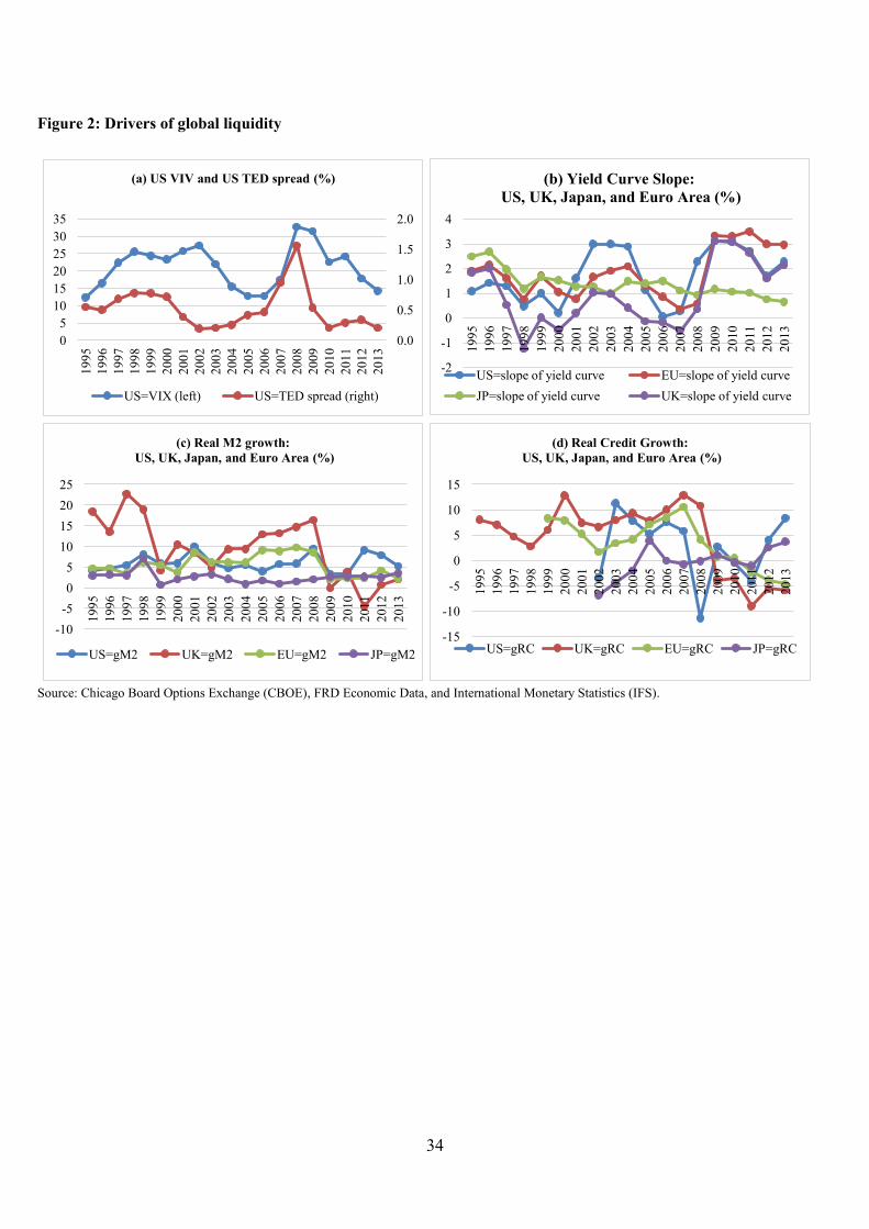
How can we measure the drivers of global liquidity? Eickmeier et al., (2013)

measure global liquidity conditions based on the common global factors in the

dynamics of liquidity indicators of 24 advanced and emerging economies. The authors

find that the main drivers of monetary policy are the following three factors: implied

market volatility (i.e., the VIX indicator), domestic credit growth, and broad money

(M2) growth. In addition to these measures, Cerutti et al., (2014) and the IMF (2014a)

include the TED spread and the yield curve slope. The TED spread is the difference

between the short-term interest rate and government debt (risk-free asset) rates,

indicating perceived credit risk. The yield curve slope is the difference between long-

and short-term interest rates in major economies.

How can the liquidity conditions in global financial markets, that is, global

liquidity, be transmitted to other economies? The transmission of global liquidity can

be distinguished among drivers, transmission channels, and financial condition

outcomes (IMF, 2014a). The IMF (2014a) considers that ease of global finance is

driven by global financial market conditions, is transmitted internationally by the

activities of global investors and financial intermediaries, and leads to local financial

4

condition outcomes, such as credit increases and asset price rises. The transmission

channels through the activities of global investors and financial intermediaries can be

confirmed by cross-border capital flows. Shinkai and Enya (2014) examine the impacts

of capital inflows on asset prices for emerging economies in Asia. The authors find that

the impacts vary across economies and across types of capital inflows. While the

authors analyze the links between transmission channels and local financial condition

outcomes, this study examines the relationship between drivers of global liquidity and

transmission channels.

There are three different channels through which global liquidity can be

transmitted, that is, international equity portfolios, bond portfolios, and bank flows.

Some studies examine the impacts of global liquidity drivers on capital flows. The IMF

(2014a) analyzes the impacts on international portfolio and bank flows and finds that

the impacts of the VIX indicator and the TED spreads on both portfolio and bank flows

are commonly negative, while the impacts of other global variables differ by type of

cross-border flows. The yield curve slope has positive impacts on bond flows, negative

impacts on bank flows, and insignificant impacts on equity flows. The different impacts

might be caused by different channels as well as by substitution effects. Cerutti et al.,

(2014) examine the impacts of global liquidity drivers on cross-border bank flows. The

authors identify the global liquidity conditions originated by the US, UK, Japan, and

Euro Area economies as credit and M2 growth in each of the four economies. The

authors conclude that important drivers of bank flows are the financial conditions in the

UK and Euro Area rather than those in the US.

This study is similar to Cerutti et al., (2014) and the IMF (2014a). However,

this study is different in the following aspects. It uses three-dimensional (and

bidirectional) panel data, which makes it possible to examine the drivers of the capital

5

flows from economy j to economy i at time t. The impacts of global liquidity may vary

across economies owing to regional characteristics. The more economic globalization

proceeds, the more regional economic integration accelerates. In Asia, advanced and

emerging economies have become more integrated through regional trade rather than

through regional financial activities (BIS, 2008). Borensztein and Loungani (2011)

investigate the trends in financial integration within Asia based on cross-border equity

and bond holdings data in 2007. One of their main findings is that the ratio of portfolio

investments within Asia (38 percent for equity investment and 15 percent for bond

investments) is higher than the corresponding figures for Latin America (8 percent for

equity investment and 8 percent for bond investments) and Eastern Europe (18 percent

for equity investment and 9 percent for bond investments), but much lower than the

ratio of portfolio investments within industrialized countries (85 percent for equity

investment and 93 percent for bond investments).

Against this background on regional financial and economic integration, this

study focus on the regional differences in the impacts of global liquidity drivers on

capital flows, and also focuses on the relationships between the impacts and policy

responses to capital inflows. He and McCauley (2013) examine the transmission of

major economies’ monetary policy to East Asia, in particular, China, Hong Kong, and

Korea, by focusing on the channel of cross-border foreign currency credit. One of that

study’s main findings is that foreign currency credit to firms in mainland China and to

affiliates of Chinese firms in Hong Kong has been increasing very rapidly, while that to

firms in Korea has not been increasing as rapidly. In contrast to the limited growth of

foreign currency credit, the stock of foreign currency bonds on nonfinancial

corporations in Korea is growing rapidly. The limited growth of foreign currency credit

in Korea may be caused by Korean macroprudential policy (Bruno and Shin, 2013; He

6

and McCauley, 2013). These discussions suggest the impacts of global liquidity drivers

on capital flows depend not only on the conditions of donor economies but also on the

conditions of recipient economies.

III. Methodology and Data

III.1 Methodology

To examine the effects of global liquidity on capital flows, we estimate the

following basic empirical model:

= + + + + + ,

where the dependent variable is the annual log difference in the stock of cross-

border financial assets issued by recipient economy i owned in donor economy j at time

t. We focus on three types of cross-border financial assets: equities, bonds, and bank

credit. is the set of global liquidity drivers at time t. is the set of global

liquidity drivers that originate in donor economy j at time t. is the set of domestic

factors that explain the country-specific macroeconomic conditions of recipients.

captures the fixed effects of recipient economy i received from donor j. is the error

term. Donor economies are represented by the US, UK, Japan, and Euro area

economies, that is j=1,…,4 (G4 hereafter), while the recipient economies are the 91

economies in Table 1, that is, i=1,…,91. We include Euro area economies as both

recipient and donor economies; however, we define a donor Euro area economy as the

aggregated economies in the Euro area. The sample covers 12 periods from 2002 to

2013.

7

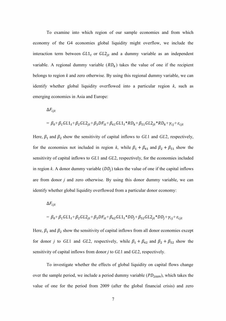
To examine into which region of our sample economies and from which

economy of the G4 economies global liquidity might overflow, we include the

interaction term between or and a dummy variable as an independent

variable. A regional dummy variable ( ) takes the value of one if the recipient

belongs to region k and zero otherwise. By using this regional dummy variable, we can

identify whether global liquidity overflowed into a particular region k, such as

emerging economies in Asia and Europe:

= + + + + * + * + +

Here, and show the sensitivity of capital inflows to GL1 and GL2, respectively,

for the economies not included in region k, while and show the

sensitivity of capital inflows to GL1 and GL2, respectively, for the economies included

in region k. A donor dummy variable ( ) takes the value of one if the capital inflows

are from donor j and zero otherwise. By using this donor dummy variable, we can

identify whether global liquidity overflowed from a particular donor economy:

= + + + + * + * + +

Here, and show the sensitivity of capital inflows from all donor economies except

for donor j to GL1 and GL2, respectively, while and show the

sensitivity of capital inflows from donor j to GL1 and GL2, respectively.

To investigate whether the effects of global liquidity on capital flows change

over the sample period, we include a period dummy variable ( ), which takes the

value of one for the period from 2009 (after the global financial crisis) and zero

8

otherwise. We can catch the structural change in the sensitivities by including the

interaction of a period dummy with a global factor (GL1 or GL2).

Moreover, to examine the relationship between the sensitivity of capital inflows

to global factor and the recipient’s policy regimes, we estimate the augmented

regression model replacing a regional dummy variable ( ) with policy regimes

characteristics variable ( ). We focus on exchange rate flexibility and capital

openness of recipient economies.

III.2 Data

The dependent variable in our basic model is the rate of change of cross-border

financial assets. Our data on cross-border financial assets are derived from the

Coordinated Portfolio Investment Survey (CPIS) provided by the IMF and the

International Banking Statistics (IBS) provided by the Bank for International

Settlements (BIS). The CPIS covers the two types of portfolio investment assets issued

by nonresidents and owned by residents: equity securities and bond securities (see

Tables 1.1 and 1.2 of the CPIS). The IBS covers cross-border bank claims in reporting

countries and consists of two datasets: locational banking statistics and consolidated

banking statistics (CBS). The latter, on which our analysis is based (see Table 9B of the

CBS), covers bilateral cross-border bank claims, although it does include the claims of

foreign affiliates.2

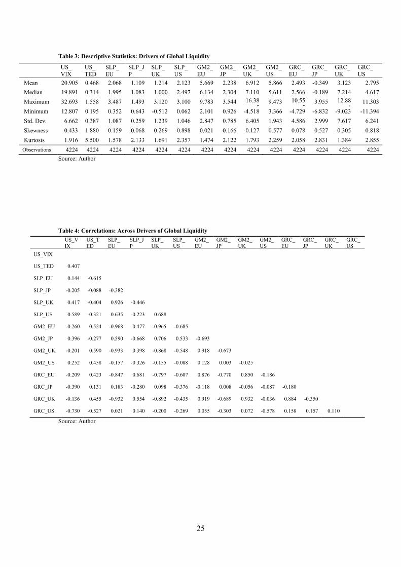
Our measures of the drivers of global liquidity are based on previous empirical

studies (IMF, 2014; Cerutti et al., 2014). We divide these drivers into global drivers

( ) and local drivers ( ). Global drivers are related to global financial

conditions, while local drivers are related to domestic economic circumstance and

9

monetary policy stances in advanced economies that affect the conditions of global

financial markets.

First, regarding global drivers ( ), we focus on the risk attitudes of global

investors and liquidity conditions of global financial markets. As a proxy of the former,

we use the CBOE volatility index (VIX), which is a key measure of the market

expectations of near-term volatility conveyed by S&P500 stock index options prices

(CBOE webpage). The VIX has been considered to reflect investors’ risk attitudes.

Hence, it tends to be low under the better liquidity conditions in global financial

markets, which encourages investment in more risky assets. The coefficient sign of the

VIX is expected to be negative.

As a proxy of the liquidity conditions in global financial markets, we use the

TED spread indicator, defined as the difference between the three-month London Inter-

Bank Offered Rate (LIBOR) and the three-month Treasury bill (T-bill) rate. T-bills are

considered risk-free assets, while the LIBOR reflects the liquidity conditions in global

financial markets. Under loose global financial market conditions, the TED spread

tends to decrease and global investors prefer more risky assets. The coefficient sign of

the TED spread must be negative.

Second, regarding regional (i.e., the donor’s own) drivers ( ), we use the

yield curve slope, M2 growth, and real credit growth indicators in the US, UK, Japan,

and Euro area economies. The slope of the yield curve is defined as the spread between

long- and short-term interest rates. Monetary easing policy makes the yield curve

steeper through a decline in short-term interest rates. Therefore, a steep slope of the

yield curve is considered to facilitate domestic investments or reduce external

investments. Hence, this coefficient sign is expected to be negative.

10

In addition, we control for how the recipient’s conditions affect capital flows in

order to identify the effects of global liquidity. We consider that global investors refer

to the recipient’s economic conditions when they decide on their investment

destinations. The variables included in our model are real GDP growth, inflation,

interest rate spread between domestic and US rates, exchange rate flexibility, financial

openness, and political stability in each recipient economy. The exchange rate

flexibility index is from the Exchange Rate Regime by Reinhart and Rogoff

Classification. Financial openness is from the Chinn–Ito Index, which is the de jure

measure of financial openness.3

The trends of capital inflows are shown in Figure 1. The averages of growth

rates of equity and bank inflows to emerging European economies are higher than

those to Asian NIES4 and ASEAN4 economies before 2007, while those of bond

inflows to emerging European economies are lower than those to Asian economies.

This trend of capital flows, however, seems to change in the opposite direction after

2008.

The global factor variables are shown in Figure 2.

IV. Empirical Results

IV.1 Main results

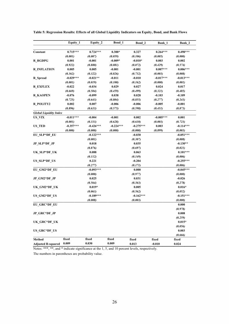
First regressions simultaneously include all drivers of global liquidity (US VIX,

US TED spread, G4 yield curve slope, G4 M2 growth, and G4 real credit growth

indicators). The results in Table 5 indicate that the US VIX remains significant with an

expected negative sign in the case of cross-border equity and bank flows, while the

TED spread remains significant in the case of cross-border bond flows. This

11

significance indicates the importance of global risk-taking attitudes in determining

cross-border equity and bank flows or that of global liquidity conditions in determining

cross-border bond flows. Moreover, G4 yield curve slopes are significant determinants

of cross-border claims on banks. However, the EU yield curve slope has an expected

highly negative sign, which signals that a steeper yield curve makes EU investors

reduce cross-border bank lending. One of the advantages of this study is its use of

bilateral data. Thus, this result suggests that the monetary institution of each country

responds to the country’s yield curve slope, not to the common US yield curve slope.

As shown in Table 5, the correlation among the individual global liquidity drivers is

negligible. Accordingly, this section compares the explanatory power of various global

liquidity factors individually.

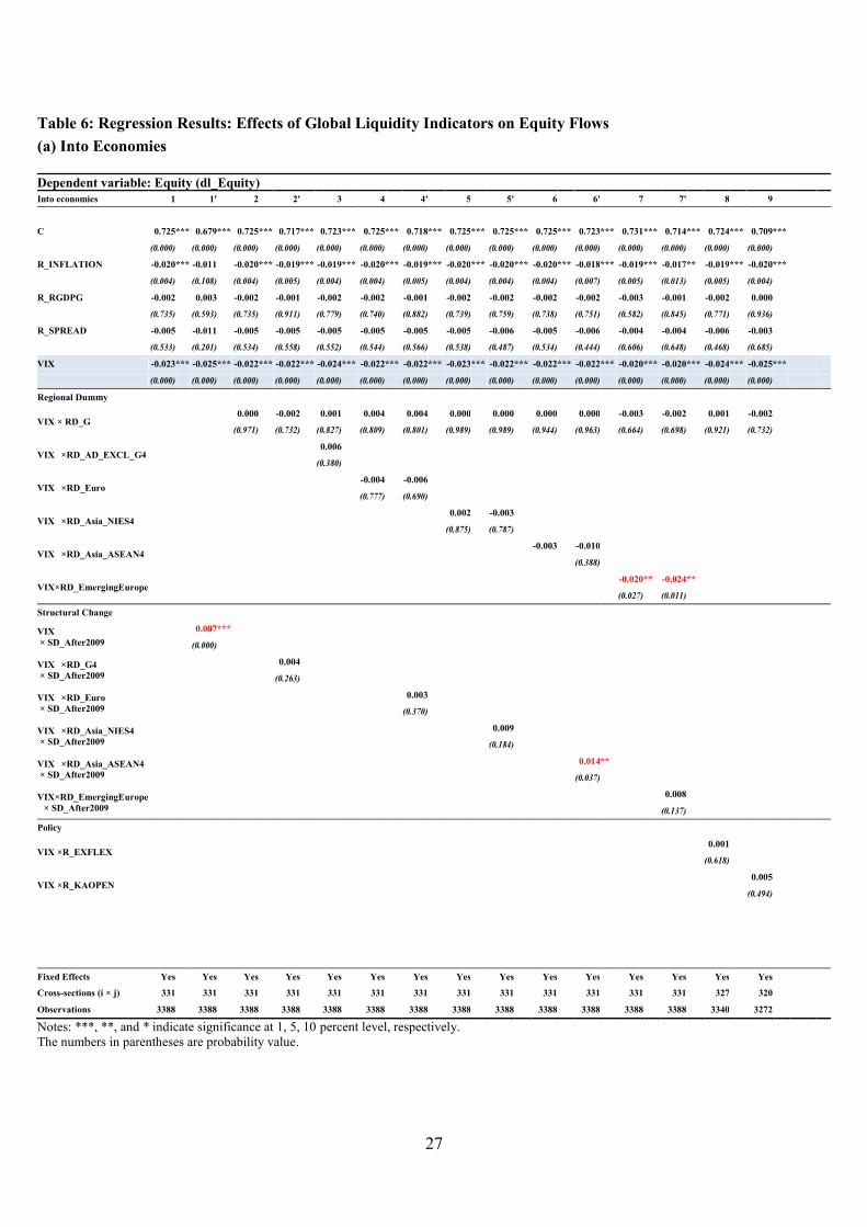
Table 6 refers to the empirical results on global equity investments. Table 6(a)

examines to which economies global liquidity is transmitted through equity flows.

Column 1 reports results from the benchmark regression. The VIX is statistically

significant with an expected negative sign, while the significance of the other global

liquidity indicators is lower than that of the VIX indicator. So, the VIX can contribute

to global equity flows as the drivers of global liquidity, suggesting that higher risk is

associated with lower growth in global equity investments. Moreover, lower inflation

can increase equity inflows. Column 1’ shows the results of augmented specification

with the VIX and its interaction with the dummy of the periods after 2009. The

interaction is positively significant, suggesting that the VIX become less sensitive to

equity flows after 2009 (the global financial crisis)..

Columns 2–7’ show the results of the augmented specification with the

interactions between the VIX and some regional dummies and their interactions with

the dummy after 2009. The coefficient of the interaction of the VIX with the regional

12

dummy of emerging Europe is significantly negative (column 7 and 7’). The equity

inflows to emerging European economies are more sensitive to global factors compared

with those to other regions during the whole period. After the global financial crisis, the

equity flows to ASEAN4 economies become less sensitive to global factors than before

(column 6 and 6’).

Column 8–9 show the results of the specification with the VIX and its

interactions with policy variables, such as exchange rate flexibility and capital openness.

We cannot find a significant result on policy variables.

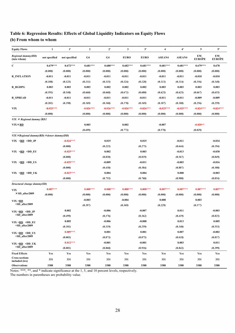
Table 6(b) examines from which economies to which economies global

liquidity is transmitted. Column 1 and column 1’ are results when the regions that

recipients belong to are not distinguished (RD = 1 for all). Column 1 shows the result

of the benchmark regression, which is equal to the column 2 of Table 6(a), while

column 1’ shows the result when the donor’s own regionality (or nationality) are

distinguished by donor dummy variable (DD). The risk attitudes of global investors are

unchanged regardless of the donor’s own regionality (or nationality) before 2009 (the

global financial crisis). The interactions of a donor’s regionality with the VIX after this

crisis suggest that such equity investors in the US and the UK after 2009 are less

sensitive to global factors compared with those before 2009 (columns 1’). Column 2-5’

are the results when the regions that recipients belong to are distinguished by regional

dummy variable (RD). There are no statistically significant differences in the

sensitivities to global factors between the equity flows from G4 economies (Japan (JP),

the economies in EURO area (EU), the US, and the UK), except for the equity flows to

emerging European economies (column 3’ and 4’). The equity flows to emerging

European economies are more sensitive to global factors than those to other regions

(column 5). Moreover, the equity flows from EU to emerging European economies

13

more sensitive to global factors compared with those from JP, US, and US before 2009

(column 5’).

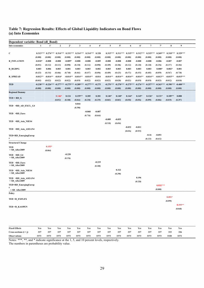
Table 7 refers to the empirical results on global bond investments. Tables 7(a)

examine to which economy global liquidity is transmitted through bond flows,

respectively. In cases of global bond investment, the US TED spread is statistically

significant with an expected negative sign (column 1 of Table 7(a)), while the other

global liquidity indicators are less significant than the US TED spread. So, the US TED

spread can contribute to global bond flows as the drivers of global liquidity, suggesting

that loose global liquidity conditions are associated with higher growth in global bond

investments. Moreover, lower inflation and a smaller interest rate spread can increase

bond inflows (column 1 of Table 7(a)). The negative sign of the interest spread is

puzzling. It may be caused by the sample coverage herein, which includes many

developing countries that have immature financial systems and government-controlled

(not market-based) interest rates.

When we consider the possibility that the G4 donors also can become recipients

of cross-border bond flows, the sensitivities of global bond inflows to global factors are

lower for the G4 recipients than that for the other recipients (column 2 of Table 7(a)).

This result suggests the existence of regional bias, that is, preference for the bonds

issued by main players in the global bond markets. After the global financial crisis,

global bond investors turn out to be less sensitive to global liquidity conditions for all

recipient countries (column 1’ of Table 7(a)), much less for emerging European

economies (column 7’ of Table 7(a)). Columns 8–9 of Table 7(a) show the results of

the specification with the VIX and its interactions with policy variables, such as

exchange rate flexibility and capital openness. We find that bond inflows to economies

with higher exchange rate flexibility are less sensitive to global factors. In addition, we

14

find that bond inflows to economies with higher capital openness are less sensitive to

global factors.

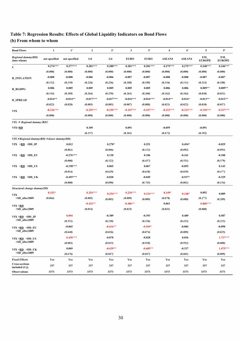
Tables 7(b) examine from which economy to which economy global liquidity is

transmitted through bond flows. UK and EU investors have higher sensitivity than JP

and US investors have during the whole period (columns 1’). Bond flows from UK to

G4 and EU are more sensitive to global factors than those from other regions to G4 and

Euro economies after 2009 (column 2’ and 3’). After 2009, Bond flows to emerging

European economies, especially bond flows from UK and US to those economies,

become less sensitive (column 5 and 5’).

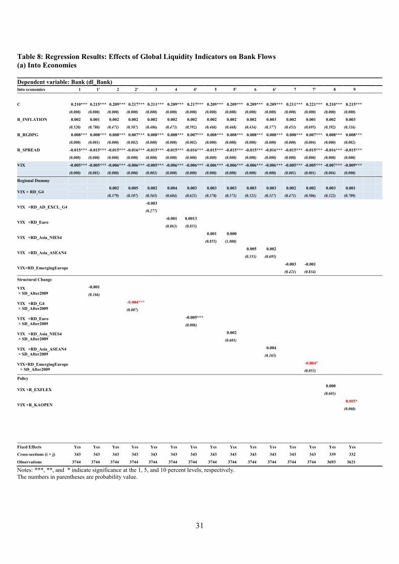
Table 8 refers to the empirical results on cross-border claims on banks. Table

8(a) examines to which economies global liquidity is transmitted through bank flows.

The US VIX is statistically significant with expected negative signs, while the other

global liquidity indicators are less significant than the VIX (column 1 of Table 8(a)).

The VIX can contribute to cross-border bank flows as the drivers of global liquidity,

suggesting that higher risk is associated with lower growth in cross-border bank

investments. Interestingly, the sensitivity of bank inflows to the VIX is smaller than

that of equity inflows (cullumn 1 in Table 6 and 8). Moreover, higher GDP growth and

a smaller interest rate spread can increase bank inflows (column 1 of Table 8(a)). Not

only global factors but also recipient’s real GDP growth plays an important role in the

driver of bank inflows.

The interactions of the VIX with some regional dummies are not significant

(column 2, 3, 4, 5, 6, and 7). However, some their interactions with period dummy of

the period after 2009 are significantly negative. The Bank inflows to G4 economies,

EURO economies, and emerging European economies become more sensitive to global

15

factors after 2009 (column 2’, 4’, and 7’). The sensitivities of the Bank inflows to

Asian economies (NIES4 and ASEAN4 economies) to global factors are not change

significantly before and after 2009 (column 5’ and 6’). Why do the sensitivities of the

bank inflows to emerging European economies to global factors become higher after

2009? The main drivers of bank inflows to emerging European economies might

change from factors other than global factors, such as recipient’s GDP growth, to

global factors before and after 2009.

Columns 8–9 of Table 8(a) show the results of the specification with the VIX

and its interactions with policy variables, such as exchange rate flexibility and capital

openness. We find that bank inflows into economies with higher capital openness are

less sensitive to global factors (column 9).

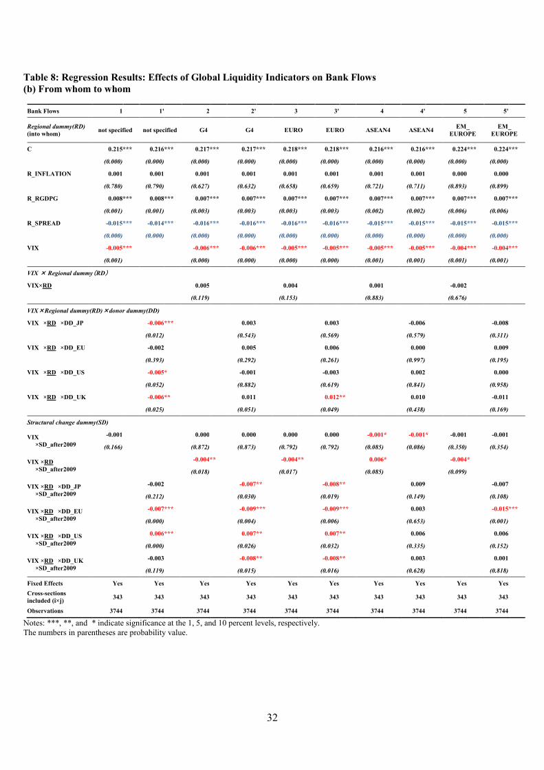
Table 8(b) examines from which economy to which economy global liquidity is

transmitted. Before 2009, although bank flows from JP and UK are sensitive to global

factors, those from EU are not sensitive (column 1’). Bank flows from EU, especially

Bank flows from EU to G4, EU, and emerging European economies, become sensitive

after 2009 (column 1’, 2’, 3’, and 5’). Bank flows from UK to G4 and EU become more

sensitive after 2009 (column 2’ and 3’). In the contrast with high sensitivity of bank

flows to G4, EURO economies, emerging European economies after 2009, the

sensitivity of bank flows to ASEAN 4 economies do not become more sensitive

(column 2’, 3’, 4’ and 5’).

Here, we summarize our main findings. From which economies and into which

economies is global liquidity transmitted through equity, bond, and bank flows during

2002–2013? For all three flow types, the sensitivity to global factors is highly

significant. Interestingly, the sensitivities depend on donor’s and recipient’s regionality

16

and change before and after 2009. The equity flows into the emerging economies in

Europe, especially equity flows from the economies in EURO area to emerging

economies in Europe, are more sensitive to global factors during 2002 to 2013 than

those to other region. The bond flows from the UK and economies in EURO area are

more sensitive while those from Japan are less sensitive during 2002 to 2009. After

2009, the bond flows from the UK and economies in EURO area to G4 economies and

economies in EURO area become more sensitive, the bond flows from the US and the

UK to emerging economies in Europe become less sensitive. Before 2009, the bank

flows from the economies in EURO area are not sensitive. After 2009, the bank flows

from the economies in the EURO area and those into the G4 economies, the economies

in EURO area, and the emerging economies in Europe become more sensitive to global

factors, while the bank flows to ASEAN 4 economies become less sensitive.

IV.2 Robustness check

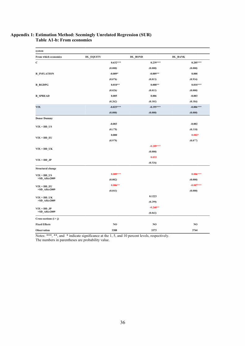
To check robustness of our main result, we estimate a SUR (Seemingly

Unrelated Regression) system. Our SUR system consists of equity, bond, and bank

flows equations. We estimate the parameters of the system, accounting for

heteroskedasticity and contemporaneous correlation in the errors across equations.

Although our dependent variables are not share but growth, the errors in three equations

assume to be correlated. Table A1-a and Table A1-b in Appendix 1 show the results of

SUR. The results imply that our main results are robust.

Table A1-a also shows that the bank inflows to emerging European economies

are more sensitive to global factors significantly than those to other economies before

2008 and after 2009 they become less sensitive significantly. On the contrary, the bank

17

inflows to emerging European economies are more sensitive significantly than those to

other economies before 2008 and after 2009 they become more sensitive significantly.

These evidences seem to reinforce our arguments. That is, not only global factors but

also factors other than global factors, such as recipient’s GDP growth might contribute

to drivers of the bank inflows to emerging European economies before 2008.

V. Concluding Remarks

This study focuses on the role of global liquidity as a driver of capital flows to

emerging/developing economies by using bilateral data, which include three types of

capital flows, namely, global equity investment, bond investment, and bank lending.

According to global equity and bank investments, the VIX turns out to be recognized as

a global liquidity index. According to global bond investments, the TED spread is

confirmed to be a global liquidity index. In other words, global equity investors are

sensitive to risk attitudes, global bond investors are sensitive to global liquidity

conditions, and global bank lenders are sensitive to risk attitudes and donors’ own

macroeconomic conditions. The US, Euro area, UK, and Japan are central in current

global equity, bond, and bank networks, and so, global portfolio inflows are strongly

involved with global financial conditions, which are determined by these countries’

own macroeconomic policies and conditions. As a result, we conclude that the drivers

of capital flows and their relative importance vary with (1) the type of fund flows, (2)

G4 (donors’) and recipients’ characteristics, and (3) G4 macroeconomic policies. The

unconventional monetary policies implemented by G4 after the global financial crisis

caused spillover effects on the emerging economies through international financial

linkages. Ghosh et al. (2014) showed with the different method of estimation that

18

capital flows to emerging economies turned out to be volatile after this crisis and that

global factors act as gatekeepers, determining when surges to Emerging economies

occur. This result seems to be consistent with our results.

Which is better for recipient economy, more or less sensitive of capital inflows

to global factors? High sensitivity implies high vulnerability to global shocks. So,

policy makers in emerging economies prefer less sensitive to global factors. However,

this study shows that the sensitivities of bank inflows become higher after 2009 for

Euro members and emerging European economies, while those remain unchanged for

Asian NIES4 and ASEAN4 economies. What is the cause of this difference? We will

defer a critical examination of this question to future research, but offer some

speculative answers here.

Firstly, the stronger policy responses in Asia could be one reason. Some strong

policy responses, such as policy rate changes, macroprudential tools, and capital

controls, are effective for capital surge shocks (He and McCauley, 2013, Bruno and

Shin, 2013, IMF, 2014b). As an empirical example, Ostry et al. (2012) indicate that

capital controls and various prudential policies can help mitigate the damage that may

occur during busts by reducing the riskiness of external liability structures. However,

this paper lets us aware the importance of understanding carefully the mechanism of

capital flows before executing the capital controls and various prudential policies.

Although this study examines the effects of recipient’s policy regimes on capital

inflows, their effects can not be clarified.

Secondly, they could be caused by the issues on regional economic integrations.

The economic integration in Asia has deepened with the development of the

international production network. The development of the international production

19

network has had impact on the capital inflows to the economies in Asia. The

multinational corporations has strengthen internal finance, that is own savings and

intra-firm financing with their headquarters at home, rather than external finance

(Kohsaka, 2015). So, the ratio of foreign direct investment type inflows to capital

inflows has risen in Asia. However, the lesson from the Asian financial crisis reduced

the interest of portfolio and bank inflows which may be less sensitive to global factors

than these inflows to the emerging economies in Europe.

20

Footnotes

1 The economies covered in this study are shown in Table 1.

2 Table 9B of the CBS presents foreign claims by the nationality of the reporting bank

on an immediate borrower basis, which includes both cross-border international claims

and local claims in the local currency by a particular country.

3 For more details, refer to Chinn and Ito (2008).

21

References

BIS (Bank of International Settlements), 2008, Regional Financial Integration in Asia:

Present and Future, BIS Papers, No. 42.

BIS (Bank of International Settlements), 2014, The Transmission of Unconventional

Monetary Policy to the Emerging Markets, BIS Papers, No. 78.

Borensztein, E. and P. Loungani, 2011, Asian Financial Integration: Trends and

Interruptions. IMF Working Paper, WP/11/4.

Borio, C., 2008, The Financial Turmoil of 2007–?: A Preliminary Assessment and

Some Policy Considerations. BIS Working Papers, No.251.

Bruno, V. and H. S. Shin, 2013, Assessing Macroprudential Policies: Case of Korea.

NBER Working Paper Series, No. 19084.

Cerutti, E., S. Claessens and L. Ratnovski, 2014, Global Liquidity and Drivers of

Cross-Border Bank Flows. IMF Working Paper, WP/14/69.

Chinn, M. and H. Ito, 2008, A new measure of financial openness. Journal of

Comparative Policy Analysis, 10(3), pp. 309–322.

CGFS (Committee on the Global Financial System), 2011, Global Liquidity—Concept,

Measurement and Policy Implications. CGFS Papers, No. 45.

De Almedia, L. A., 2015, A Network Analysis of Sectoral Accounts: Identifying

Sectoral Interlinkages in G-4 Economies. IMF Working Paper, WP/15/111.

Eickmeier, S., L. Gambacorta and B. Hofmann, 2013, Understanding Global Liquidity.

BIS Working Papers, No. 402.

22

Ghosh, A. R., M. S. Qureshi, J. I. Kim and J. Zalduendo, 2014, Surges. Journal of

International Economics, Vol. 92(2), pp. 266-285.

He, D. and R. N. McCauley, 2013, Transmitting Global Liquidity to East Asia: Policy

Rates, Bond Yields, Currencies and Dollar Credit. BIS Working Paper, No. 431.

IMF (International Monetary Fund), 2010, Global Liquidity Expansion: Effects on

“Receiving” Economies and Policy Response Options. Global Financial Stability

Report, Chapter 4, pp. 327–354.

IMF (International Monetary Fund), 2014a, Global Liquidity: Issues for Surveillance.

IMF Policy Paper.

IMF (International Monetary Fund), 2014b, World Economic Outlook, October 2014, p.

xiii.

Kohsaka, Akira, 2015, Macro-financial Linkages and Financial Deepening: An

overview. Akira Kohsaka (ed.), Macro-Financial Linkages in the Pacific Region,

Chapter 1, pp.15-38, Routledge.

Ostry, J.D., A.R. Ghosh, M. Chamon and M. S. Qureshi, 2012, Tools for managing

financial-stability risks from capital inflows. Journal of International Economics,

Vol. 88(2), pp. 407-421.

Quinn, D., M. Schindler and A. M. Toyoda, 2011, Assessing measures of financial

integration and openness. IMF Economic Review, 59(3), pp. 488–523.

Shinkai, J. and M. Enya, 2014, The Impact of Capital Inflows on Asset Prices in East

Asia. Discussion Paper Series, No. 22, Kanazawa University.

23

Table 1: Regional Distributions of Sample Economies

Asia (17) Europe (32)

Africa (16)

Other regions (26)

Advanced economies Advanced economies United Kingdom

Cameroon Advanced economies

Japan * Czech Republic Congo, Republic of United States *

Hong Kong (N) Denmark Cote d’Ivoire Australia

Korea (N) Iceland Egypt Canada

Singapore (N) Norway Gabon Israel

Taiwan (N) Sweden Gambia, The New Zealand

Switzerland Ghana

Emerging and

developing

United Kingdom Kenya Emerging and developing

Euro Area(16) * Liberia

Bangladesh Austria Mali Argentina

China PR: Mainland Belgium Mauritius Bahamas, The

China, PR: Macao Cyprus Morocco Bahrain, Kingdom of

India Estonia Namibia Barbados

Indonesia (A) Finland Nigeria Belize

Lao People’s Democratic

Republic

France South Africa Botswana

Malaysia (A) Germany Zambia Brazil

Pakistan Greece Chile

Philippines (A) Ireland Colombia

Sri Lanka Italy Georgia

Thailand (A) Luxembourg Jordan

Vietnam Malta Kuwait

Netherlands Lebanon

Portugal Mexico

Slovenia Oman

Spain Panama

Papua New Guinea

Emerging and

developing

Peru

Russian Federation

Bulgaria (EE) Saudi Arabia

Croatia (EE) Venezuela

Hungary (EE)

Latvia (EE)

Lithuania (EE)

Poland (EE)

Romania (EE)

Turkey (EE)

Ukraine (EE)

Source: Author

Notes: Country classification is based on the IMF’s World Economic Outlook.

* represents donor economies. namely, Japan, the UK, Euro area, and US. (N) represents the newly

industrialized economies’ dummy economies (NIES4), comprising Hong Kong, Korea, Singapore, and

Taiwan. (A) represents the ASEAN4 dummy economies, namely, Indonesia, Malaysia, the Philippines, and

Thailand. (EE) represents emerging economies in Europe dummy, namely Bulgaria, Croatia, Hungary,

Latvia, Lithuania, Poland, Romania, Turkey, and Ukraine.

24

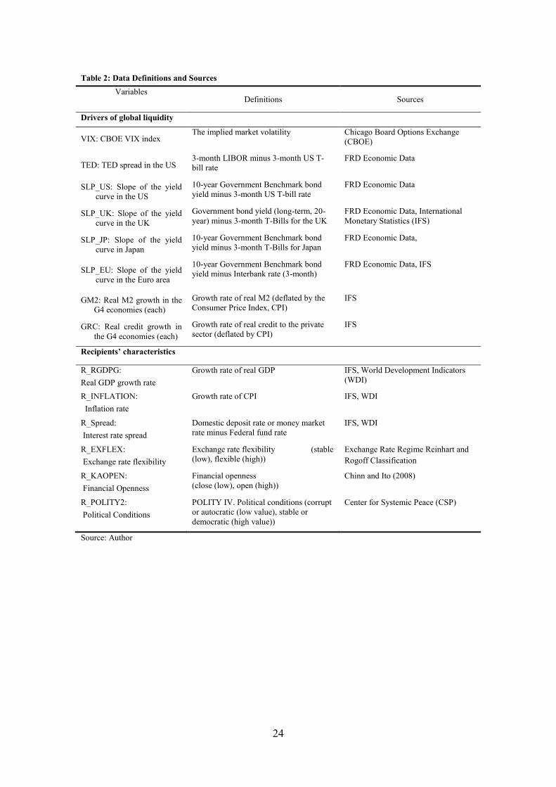
Table 2: Data Definitions and Sources

Variables Definitions Sources

Drivers of global liquidity

VIX: CBOE VIX index The implied market volatility Chicago Board Options Exchange

(CBOE)

TED: TED spread in the US 3-month LIBOR minus 3-month US T-

bill rate

FRD Economic Data

SLP_US: Slope of the yield

curve in the US

10-year Government Benchmark bond

yield minus 3-month US T-bill rate

FRD Economic Data

SLP_UK: Slope of the yield

curve in the UK

Government bond yield (long-term, 20-

year) minus 3-month T-Bills for the UK

FRD Economic Data, International

Monetary Statistics (IFS)

SLP_JP: Slope of the yield

curve in Japan


yield minus 3-month T-Bills for Japan

FRD Economic Data,

SLP_EU: Slope of the yield

curve in the Euro area


yield minus Interbank rate (3-month)

FRD Economic Data, IFS

GM2: Real M2 growth in the

G4 economies (each)

Growth rate of real M2 (deflated by the

Consumer Price Index, CPI)

IFS

GRC: Real credit growth in

the G4 economies (each)

Growth rate of real credit to the private

sector (deflated by CPI)

IFS

Recipients’ characteristics

R_RGDPG:

Real GDP growth rate

Growth rate of real GDP IFS, World Development Indicators

(WDI)

R_INFLATION:

Inflation rate

Growth rate of CPI IFS, WDI

R_Spread:

Interest rate spread

Domestic deposit rate or money market

rate minus Federal fund rate

IFS, WDI

R_EXFLEX:

Exchange rate flexibility

Exchange rate flexibility (stable

(low), flexible (high))

Exchange Rate Regime Reinhart and

Rogoff Classification

R_KAOPEN:

Financial Openness

Financial openness

(close (low), open (high))

Chinn and Ito (2008)

R_POLITY2:

Political Conditions

POLITY IV. Political conditions (corrupt

or autocratic (low value), stable or

democratic (high value))

Center for Systemic Peace (CSP)

Source: Author

25

Table 3: Descriptive Statistics: Drivers of Global Liquidity

Source: Author

Table 4: Correlations: Across Drivers of Global Liquidity

US_V

IX

US_T

ED

SLP_

EU

SLP_J

P

SLP_

UK

SLP_

US

GM2_

EU

GM2_

JP

GM2_

UK

GM2_

US

GRC_

EU

GRC_

JP

GRC_

UK

GRC_

US

US_VIX

US_TED 0.407

SLP_EU 0.144 -0.615

SLP_JP -0.205 -0.088 -0.382

SLP_UK 0.417 -0.404 0.926 -0.446

SLP_US 0.589 -0.321 0.635 -0.223 0.688

GM2_EU -0.260 0.524 -0.968 0.477 -0.965 -0.685

GM2_JP 0.396 -0.277 0.590 -0.668 0.706 0.533 -0.693

GM2_UK -0.201 0.590 -0.933 0.398 -0.868 -0.548 0.918 -0.673

GM2_US 0.252 0.458 -0.157 -0.326 -0.155 -0.088 0.128 0.003 -0.025

GRC_EU -0.209 0.423 -0.847 0.681 -0.797 -0.607 0.876 -0.770 0.850 -0.186

GRC_JP -0.390 0.131 0.183 -0.280 0.098 -0.376 -0.118 0.008 -0.056 -0.087 -0.180

GRC_UK -0.136 0.455 -0.932 0.554 -0.892 -0.435 0.919 -0.689 0.932 -0.036 0.884 -0.350

GRC_US -0.730 -0.527 0.021 0.140 -0.200 -0.269 0.055 -0.303 0.072 -0.578 0.158 0.157 0.110

Source: Author

US_

VIX

US_

TED

SLP_

EU

SLP_J

P

SLP_

UK

SLP_

US

GM2_

EU

GM2_

JP

GM2_

UK

GM2_

US

GRC_

EU

GRC_

JP

GRC_

UK

GRC_

US

Mean 20.905 0.468 2.068 1.109 1.214 2.123 5.669 2.238 6.912 5.866 2.493 -0.349 3.123 2.795

Median 19.891 0.314 1.995 1.083 1.000 2.497 6.134 2.304 7.110 5.611 2.566 -0.189 7.214 4.617

Maximum 32.693 1.558 3.487 1.493 3.120 3.100 9.783 3.544 16.38

5 9.473 10.55

5 3.955 12.88

4 11.303

Minimum 12.807 0.195 0.352 0.643 -0.512 0.062 2.101 0.926 -4.518 3.366 -4.729 -6.832 -9.023 -11.394

Std. Dev. 6.662 0.387 1.087 0.259 1.239 1.046 2.847 0.785 6.405 1.943 4.586 2.999 7.617 6.241

Skewness 0.433 1.880 -0.159 -0.068 0.269 -0.898 0.021 -0.166 -0.127 0.577 0.078 -0.527 -0.305 -0.818

Kurtosis 1.916 5.500 1.578 2.133 1.691 2.357 1.474 2.122 1.793 2.259 2.058 2.831 1.384 2.855

Observations 4224 4224 4224 4224 4224 4224 4224 4224 4224 4224 4224 4224 4224 4224

26

Table 5: Regression Results: Effects of all Global Liquidity Indicators on Equity, Bond, and Bank Flows

Equity_1 Equity_2 Bond_1 Bond_2 Bank_1 Bank_2

Constant 0.715 *** 0.724 *** 0.300 * 0.327 0.264 *** 0.498 ***

(0.001) (0.007) (0.059) (0.106) (0.005) (0.000)

R_RGDPG 0.001 -0.001 -0.009 * -0.010 * 0.003 0.002

(0.922) (0.880) (0.081) (0.072) (0.429) (0.574)

R_INFLATION 0.005 0.005 -0.001 -0.001 0.007 *** 0.006 ***

(0.362) (0.322) (0.826) (0.732) (0.003) (0.008)

R_Spread -0.029 *** -0.021 ** -0.011 -0.010 -0.017 *** -0.013 ***

(0.001) (0.019) (0.100) (0.162) (0.000) (0.001)

R_EXFLEX -0.022 -0.034 0.029 0.027 0.024 0.017

(0.669) (0.504) (0.459) (0.499) (0.321) (0.485)

R_KAOPEN -0.076 -0.099 0.038 0.028 -0.103 -0.109

(0.725) (0.643) (0.804) (0.855) (0.277) (0.243)

R_POLITY2 0.002 0.007 -0.006 -0.006 -0.005 -0.001

(0.896) (0.633) (0.575) (0.598) (0.451) (0.873)

Global Liquidity Index

US_VIX -0.011 *** -0.004 -0.001 0.002 -0.005 *** 0.001

(0.001) (0.333) (0.628) (0.610) (0.003) (0.723)

US_TED -0.357 *** -0.426 *** -0.224 *** -0.275 *** 0.003 -0.114 ***

(0.000) (0.000) (0.000) (0.000) (0.899) (0.003)

EU_SLP*DF_EU -0.122 *** -0.030 -0.051 ***

(0.001) (0.307) (0.008)

JP_SLP*DF_JP 0.018 0.035 -0.130 **

(0.876) (0.697) (0.021)

UK_SLP*DF_UK 0.088 0.063 0.101 ***

(0.112) (0.149) (0.006)

US_SLP*DF_US 0.221 -0.204 -0.255 ***

(0.277) (0.171) (0.006)

EU_GM2*DF_EU -0.093 *** 0.000 -0.045 ***

(0.000) (0.977) (0.000)

JP_GM2*DF_JP 0.025 0.031 -0.026

(0.564) (0.363) (0.278)

UK_GM2*DF_UK 0.019 * 0.005 0.016 *

(0.063) (0.562) (0.052)

US_GM2*DF_US -0.189 *** -0.162 *** -0.151 ***

(0.008) (0.003) (0.000)

EU_GRC*DF_EU 0.000

(0.978)

JP_GRC*DF_JP 0.008

(0.259)

UK_GRC*DF_UK 0.015 *

(0.056)

US_GRC*DF_US 0.003

(0.666)

Method fixed fixed fixed fixed fixed fixed

Adjusted R-squared 0.009 0.030 0.009 0.013 -0.010 0.024

Notes: ***, **, and * indicate significance at the 1, 5, and 10 percent levels, respectively.

The numbers in parentheses are probability value.

27

Table 6: Regression Results: Effects of Global Liquidity Indicators on Equity Flows

(a) Into Economies

Dependent variable: Equity (dl_Equity)

Into economies 1 1' 2 2' 3 4 4' 5 5' 6 6' 7 7' 8 9

C 0.725 *** 0.679 *** 0.725 *** 0.717 *** 0.723 *** 0.725 *** 0.718 *** 0.725 *** 0.725 *** 0.725 *** 0.723 *** 0.731 *** 0.714 *** 0.724 *** 0.709 ***

(0.000) (0.000) (0.000) (0.000) (0.000) (0.000) (0.000) (0.000) (0.000) (0.000) (0.000) (0.000) (0.000) (0.000) (0.000)

R_INFLATION -0.020 *** -0.011 -0.020 *** -0.019 *** -0.019 *** -0.020 *** -0.019 *** -0.020 *** -0.020 *** -0.020 *** -0.018 *** -0.019 *** -0.017 ** -0.019 *** -0.020 ***

(0.004) (0.108) (0.004) (0.005) (0.004) (0.004) (0.005) (0.004) (0.004) (0.004) (0.007) (0.005) (0.013) (0.005) (0.004)

R_RGDPG -0.002 0.003 -0.002 -0.001 -0.002 -0.002 -0.001 -0.002 -0.002 -0.002 -0.002 -0.003 -0.001 -0.002 0.000

(0.735) (0.593) (0.735) (0.911) (0.779) (0.740) (0.882) (0.739) (0.759) (0.738) (0.751) (0.582) (0.845) (0.771) (0.936)

R_SPREAD -0.005 -0.011 -0.005 -0.005 -0.005 -0.005 -0.005 -0.005 -0.006 -0.005 -0.006 -0.004 -0.004 -0.006 -0.003

(0.533) (0.201) (0.534) (0.558) (0.552) (0.544) (0.566) (0.538) (0.487) (0.534) (0.444) (0.606) (0.648) (0.468) (0.685)

VIX -0.023 *** -0.025 *** -0.022 *** -0.022 *** -0.024 *** -0.022 *** -0.022 *** -0.023 *** -0.022 *** -0.022 *** -0.022 *** -0.020 *** -0.020 *** -0.024 *** -0.025 ***

(0.000) (0.000) (0.000) (0.000) (0.000) (0.000) (0.000) (0.000) (0.000) (0.000) (0.000) (0.000) (0.000) (0.000) (0.000)

Regional Dummy

VIX × RD_G 0.000 -0.002 0.001 0.004 0.004 0.000 0.000 0.000 0.000 -0.003 -0.002 0.001 -0.002

(0.971) (0.732) (0.827) (0.809) (0.801) (0.989) (0.989) (0.944) (0.963) (0.664) (0.698) (0.921) (0.732)

VIX ×RD_AD_EXCL_G4 0.006

(0.380)

VIX ×RD_Euro -0.004 -0.006

(0.777) (0.690)

VIX ×RD_Asia_NIES4 0.002 -0.003

(0.875) (0.787)

VIX ×RD_Asia_ASEAN4 -0.003 -0.010

(0.388)

VIX×RD_EmergingEurope -0.020 ** -0.024 **

(0.027) (0.011)

Structural Change

VIX

× SD_After2009

0.007 ***

(0.000)

VIX ×RD_G4

× SD_After2009

0.004

(0.263)

VIX ×RD_Euro

× SD_After2009

0.003

(0.370)

VIX ×RD_Asia_NIES4

× SD_After2009

0.009

(0.184)

VIX ×RD_Asia_ASEAN4

× SD_After2009

0.014 **

(0.037)

VIX×RD_EmergingEurope

× SD_After2009

0.008

(0.137)

Policy

VIX ×R_EXFLEX 0.001

(0.618)

VIX ×R_KAOPEN 0.005

(0.494)

Fixed Effects Yes Yes Yes Yes Yes Yes Yes Yes Yes Yes Yes Yes Yes Yes Yes

Cross-sections (i × j) 331 331 331 331 331 331 331 331 331 331 331 331 331 327 320

Observations 3388 3388 3388 3388 3388 3388 3388 3388 3388 3388 3388 3388 3388 3340 3272

Notes: ***, **, and * indicate significance at 1, 5, 10 percent level, respectively.

The numbers in parentheses are probability value.

28

Table 6: Regression Results: Effects of Global Liquidity Indicators on Equity Flows

(b) From whom to whom

Equity Flows 1 1' 2 2' 3 3' 4 4' 5 5'

Regional dummy(RD)

(into whom) not specified not specified G4 G4 EURO EURO ASEAN4 ASEAN4

EM_

EUROPE

EM_

EUROPE

C 0.679 *** 0.672 *** 0.681 *** 0.680 *** 0.682 *** 0.681 *** 0.681 *** 0.681 *** 0.679 *** 0.678

(0.000) (0.000) (0.000) (0.000) (0.000) (0.000) (0.000) (0.000) (0.000) (0.000)

R_INFLATION -0.011 -0.011 -0.011 -0.011 -0.011 -0.011 -0.011 -0.011 -0.010 -0.010

(0.108) (0.125) (0.131) (0.135) (0.124) (0.128) (0.113) (0.114) (0.156) (0.148)

R_RGDPG 0.003 0.003 0.003 0.002 0.002 0.002 0.003 0.003 0.003 0.003

(0.593) (0.548) (0.660) (0.668) (0.671) (0.680) (0.625) (0.625) (0.667) (0.655)

R_SPREAD -0.011 -0.011 -0.011 -0.011 -0.011 -0.011 -0.011 -0.011 -0.009 -0.009

(0.201) (0.198) (0.169) (0.168) (0.170) (0.169) (0.187) (0.188) (0.256) (0.259)

VIX -0.025 *** -0.026 *** -0.026 *** -0.026 *** -0.026 *** -0.025 *** -0.025 *** -0.024 *** -0.024 ***

(0.000) (0.000) (0.000) (0.000) (0.000) (0.000) (0.000) (0.000) (0.000)

VIX × Regional dummy（RD）

VIX×RD 0.003 0.002 -0.007 -0.020 **

(0.699) (0.773) (0.570) (0.029)

VIX×Regional dummy(RD)×donor dummy(DD)

VIX ×RD ×DD_JP -0.024 *** 0.015 0.015 -0.011 -0.034

(0.000) (0.225) (0.275) (0.644) (0.194)

VIX ×RD ×DD_EU -0.025 *** 0.002 0.003 -0.013 -0.030

(0.000) (0.830) (0.819) (0.567) (0.049)

VIX ×RD ×DD_US -0.029 *** -0.009 -0.011 -0.003 -0.016

(0.000) (0.438) (0.384) (0.887) (0.308)

VIX ×RD ×DD_UK -0.023 *** 0.004 0.004 0.000 -0.003

(0.000) (0.755) (0.768) (0.988) (0.854)

Structural change dummy(SD)

VIX

×SD_after2009

0.007 *** 0.008 *** 0.008 *** 0.008 *** 0.008 *** 0.007 *** 0.007 *** 0.007 *** 0.007 ***

(0.000) (0.000) (0.000) (0.000) (0.000) (0.000) (0.000) (0.000) (0.000)

VIX ×RD

×SD_after2009

-0.003 -0.004 0.008 0.003

(0.397) (0.369) (0.229) (0.577)

VIX ×RD ×DD_JP

×SD_after2009

0.002 -0.006 -0.007 0.011 -0.003

(0.499) (0.376) (0.362) (0.419) (0.825)

VIX ×RD ×DD_EU

×SD_after2009

0.005 -0.006 -0.008 0.013 0.005

(0.101) (0.319) (0.259) (0.340) (0.553)

VIX ×RD ×DD_US

×SD_after2009

0.009 *** 0.001 0.001 0.007 -0.002

(0.003) (0.873) (0.875) (0.618) (0.837)

VIX ×RD ×DD_UK

×SD_after2009

0.012 *** -0.001 -0.001 0.003 0.011

(0.001) (0.868) (0.916) (0.842) (0.299)

Fixed Effects Yes Yes Yes Yes Yes Yes Yes Yes Yes Yes

Cross-sections

included (iro) 331 331 331 331 331 331 331 331 331 331

Observations 3388 3388 3388 3388 3388 3388 3388 3388 3388 3388

Notes: ***, **, and * indicate significance at the 1, 5, and 10 percent levels, respectively. The numbers in parentheses are probability value.

29

Table 7: Regression Results: Effects of Global Liquidity Indicators on Bond Flows

(a) Into Economies

Dependent variable: Bond (dl_Bond)

Into economies 1 1' 2 2' 3 4 4' 5 5' 6 6' 7 7' 8 9

C 0.313 *** 0.274 *** 0.314 *** 0.331 *** 0.314 *** 0.314 *** 0.328 0.315 *** 0.311 *** 0.315 *** 0.312 *** 0.315 *** 0.269 *** 0.318 *** 0.329 ***

(0.000) (0.000) (0.000) (0.000) (0.000) (0.000) (0.000) (0.000) (0.000) (0.000) (0.000) (0.000) (0.000) (0.000) (0.000)

R_INFLATION -0.010 * -0.008 -0.008 -0.009 * -0.008 -0.008 -0.009 -0.008 -0.008 -0.008 -0.008 -0.008 -0.006 -0.007 -0.007

(0.051) (0.112) (0.113) (0.090) (0.130) (0.112) (0.090) (0.109) (0.106) (0.112) (0.128) (0.128) (0.256) (0.157) (0.184)

R_RGDPG 0.003 0.006 0.003 0.001 0.003 0.003 0.002 0.003 0.003 0.003 0.003 0.003 0.008 * 0.002 * 0.001

(0.425) (0.154) (0.466) (0.740) (0.461) (0.457) (0.696) (0.489) (0.425) (0.471) (0.455) (0.485) (0.059) (0.567) (0.730)

R_SPREAD -0.012 ** -0.014 ** -0.014 * -0.014 ** -0.014 ** -0.014 ** -0.014 -0.014 ** -0.014 ** -0.014 ** -0.014 ** -0.014 ** -0.013 ** -0.015 ** -0.015 ***

(0.045) (0.022) (0.022) (0.022) (0.019) (0.022) (0.023) (0.021) (0.020) (0.021) (0.019) (0.019) (0.025) (0.012) (0.010)

TED -0.238 *** -0.226 *** -0.277 *** -0.275 *** -0.289 *** -0.277 *** -0.275 -0.270 *** -0.270 *** -0.275 *** -0.276 *** -0.257 *** -0.263 *** -0.390 *** -0.408 ***

(0.000) (0.000) (0.000) (0.000) (0.000) (0.000) (0.000) (0.000) (0.000) (0.000) (0.000) (0.000) (0.000) (0.000) (0.000)

Regional Dummy

TED × RD_G 0.146 * 0.124 0.159 ** 0.205 0.201 0.140 * 0.140 * 0.144 * 0.145 * 0.126 * 0.131 * 0.189 ** 0.088

(0.052) (0.108) (0.044) (0.250) (0.259) (0.065) (0.065) (0.058) (0.056) (0.099) (0.084) (0.019) (0.297)

TED ×RD_AD_EXCL_G4 0.044

(0.590)

TED ×RD_Euro -0.068 -0.087

(0.716) (0.644)

TED ×RD_Asia_NIES4 -0.089 -0.055

(0.518) (0.694)

TED ×RD_Asia_ASEAN4 -0.032 -0.011

(0.816) (0.935)

TED×RD_EmergingEurop

e

-0.16 -0.051

(0.125) (0.632)

Structural Change

TED

× SD_After2009

0.153 *

(0.064)

TED ×RD_G4

× SD_After2009

-0.220

(0.156)

TED ×RD_Euro

× SD_After2009

-0.219

(0.188)

TED ×RD_Asia_NIES4

× SD_After2009

0.322

(0.290)

TED ×RD_Asia_ASEAN4

× SD_After2009

0.196

(0.520)

TED×RD_EmergingEurop

e

× SD_After2009

0.932 ***

(0.000)

Policy

TED ×R_EXFLEX 0.051 *

(0.099)

TED ×R_KAOPEN 0.193 **

(0.048)



Observations 3373 3373 3373 3373 3373 3373 3373 3373 3373 3373 3373 3373 3373 3328 3272


30

Table 7: Regression Results: Effects of Global Liquidity Indicators on Bond Flows


Bond Flows 1 1' 2 2' 3 3' 4 4' 5 5'

Regional dummy(RD)


EM_

EUROPE

EM_

EUROPE

C 0.274 *** 0.277 *** 0.281 *** 0.280 *** 0.281 *** 0.281 *** 0.275 *** 0.275 *** 0.248 *** 0.246 ***

(0.000) (0.000) (0.000) (0.000) (0.000) (0.000) (0.000) (0.000) (0.000) (0.000)

R_INFLATION -0.008 -0.008 -0.006 -0.006 -0.007 -0.007 -0.008 -0.008 -0.007 -0.007

(0.112) (0.139) (0.226) (0.226) (0.188) (0.189) (0.116) (0.111) (0.214) (0.188)

R_RGDPG 0.006 0.005 0.005 0.005 0.005 0.005 0.006 0.006 0.009 ** 0.009 **

(0.154) (0.189) (0.264) (0.259) (0.263) (0.260) (0.162) (0.164) (0.030) (0.031)

R_SPREAD -0.014 ** -0.014 ** -0.017 *** -0.017 *** -0.016 *** -0.016 *** -0.014 ** -0.014 * -0.013 ** -0.012 **

(0.022) (0.020) (0.005) (0.005) (0.007) (0.008) (0.021) (0.022) (0.030) (0.037)

VIX -0.226 *** -0.255 *** -0.255 *** -0.247 *** -0.247 *** -0.223 *** -0.223 *** -0.218 *** -0.217 ***

(0.000) (0.000) (0.000) (0.000) (0.000) (0.000) (0.000) (0.000) (0.000)


VIX×RD 0.109 0.091 -0.059 -0.091

(0.157) (0.261) (0.672) (0.392)


VIX ×RD ×DD_JP 0.012 0.270 * 0.251 0.454 * -0.029

(0.861) (0.066) (0.112) (0.092) (0.893)

VIX ×RD ×DD_EU -0.276 *** 0.130 0.106 -0.161 -0.100

(0.000) (0.322) (0.457) (0.551) (0.579)

VIX ×RD ×DD_US -0.158 *** 0.065 0.067 -0.055 0.143

(0.014) (0.629) (0.638) (0.839) (0.477)

VIX ×RD ×DD_UK -0.455 *** -0.020 -0.049 -0.537 * -0.329

(0.000) (0.890) (0.745) (0.061) (0.154)


VIX

×SD_after2009

0.153 * 0.254 *** 0.254 *** 0.234 *** 0.234 *** 0.149 * 0.148 * 0.092 0.089

(0.064) (0.005) (0.005) (0.009) (0.009) (0.078) (0.080) (0.277) (0.289)

VIX ×RD

×SD_after2009

-0.423 ** -0.406 ** 0.063 0.868 ***

(0.014) (0.025) (0.841) (0.000)

VIX ×RD ×DD_JP

×SD_after2009

0.094 -0.389 -0.393 0.489 0.587

(0.551) (0.228) (0.256) (0.415) (0.215)

VIX ×RD ×DD_EU

×SD_after2009

-0.065 -0.616 ** -0.569 * -0.084 -0.090

(0.640) (0.036) (0.074) (0.889) (0.825)

VIX ×RD ×DD_US

×SD_after2009

0.430 *** -0.070 -0.028 0.036 1.717 ***

(0.003) (0.815) (0.930) (0.952) (0.000)

VIX ×RD ×DD_UK

×SD_after2009

0.069 -0.639 ** -0.685 ** -0.337 1.475 ***

(0.676) (0.047) (0.047) (0.601) (0.009)


Cross-sections

included (i×j) 337 337 337 337 337 337 337 337 337 337

Observations 3373 3373 3373 3373 3373 3373 3373 3373 3373 3373

31

Table 8: Regression Results: Effects of Global Liquidity Indicators on Bank Flows

(a) Into Economies

Dependent variable: Bank (dl_Bank)

Into economies 1 1' 2 2' 3 4 4' 5 5' 6 6' 7 7' 8 9

C 0.210 *** 0.215 *** 0.209 *** 0.217 *** 0.211 *** 0.209 *** 0.217 *** 0.209 *** 0.209 *** 0.209 *** 0.209 *** 0.211 *** 0.221 *** 0.210 *** 0.215 ***

(0.000) (0.000) (0.000) (0.000) (0.000) (0.000) (0.000) (0.000) (0.000) (0.000) (0.000) (0.000) (0.000) (0.000) (0.000)

R_INFLATION 0.002 0.001 0.002 0.002 0.002 0.002 0.002 0.002 0.002 0.002 0.003 0.002 0.001 0.002 0.003

(0.520) (0.780) (0.471) (0.587) (0.486) (0.473) (0.592) (0.468) (0.468) (0.434) (0.377) (0.453) (0.695) (0.392) (0.316)

R_RGDPG 0.008 *** 0.008 *** 0.008 *** 0.007 *** 0.008 *** 0.008 *** 0.007 *** 0.008 *** 0.008 *** 0.008 *** 0.008 *** 0.008 *** 0.007 *** 0.008 *** 0.008 ***

(0.000) (0.001) (0.000) (0.002) (0.000) (0.000) (0.002) (0.000) (0.000) (0.000) (0.000) (0.000) (0.004) (0.000) (0.002)

R_SPREAD -0.015 *** -0.015 *** -0.015 *** -0.016 *** -0.015 *** -0.015 *** -0.016 *** -0.015 *** -0.015 *** -0.015 *** -0.016 *** -0.015 *** -0.015 *** -0.016 *** -0.015 ***

(0.000) (0.000) (0.000) (0.000) (0.000) (0.000) (0.000) (0.000) (0.000) (0.000) (0.000) (0.000) (0.000) (0.000) (0.000)

VIX -0.005 *** -0.005 *** -0.006 *** -0.006 *** -0.005 *** -0.006 *** -0.006 *** -0.006 *** -0.006 *** -0.006 *** -0.006 *** -0.005 *** -0.005 *** -0.007 *** -0.009 ***

(0.000) (0.001) (0.000) (0.000) (0.003) (0.000) (0.000) (0.000) (0.000) (0.000) (0.000) (0.001) (0.001) (0.004) (0.000)

Regional Dummy

VIX × RD_G4 0.002 0.005 0.002 0.004 0.003 0.003 0.003 0.003 0.003 0.002 0.002 0.003 0.001

(0.379) (0.107) (0.565) (0.604) (0.621) (0.370) (0.371) (0.321) (0.317) (0.471) (0.506) (0.322) (0.709)

VIX ×RD_AD_EXCL_G4 -0.003

(0.277)

VIX ×RD_Euro -0.001 0.0013

(0.863) (0.853)

VIX ×RD_Asia_NIES4 0.001 0.000

(0.855) (1.000)

VIX ×RD_Asia_ASEAN4 0.005 0.002

(0.353) (0.695)

VIX×RD_EmergingEurope -0.003 -0.001

(0.421) (0.834)

Structural Change

VIX

× SD_After2009

-0.001

(0.166)

VIX ×RD_G4

× SD_After2009

-0.004 ***

(0.007)

VIX ×RD_Euro

× SD_After2009

-0.005 ***

(0.006)

VIX ×RD_Asia_NIES4

× SD_After2009

0.002

(0.601)


× SD_After2009

0.004

(0.165)


× SD_After2009

-0.004 *

(0.053)

Policy

VIX ×R_EXFLEX 0.000

(0.603)

VIX ×R_KAOPEN 0.005 *

(0.060)



Observations 3744 3744 3744 3744 3744 3744 3744 3744 3744 3744 3744 3744 3744 3693 3621


32

Table 8: Regression Results: Effects of Global Liquidity Indicators on Bank Flows


Bank Flows 1 1' 2 2' 3 3' 4 4' 5 5'

Regional dummy(RD)


EM_

EUROPE

EM_

EUROPE

C 0.215 *** 0.216 *** 0.217 *** 0.217 *** 0.218 *** 0.218 *** 0.216 *** 0.216 *** 0.224 *** 0.224 ***

(0.000) (0.000) (0.000) (0.000) (0.000) (0.000) (0.000) (0.000) (0.000) (0.000)

R_INFLATION 0.001 0.001 0.001 0.001 0.001 0.001 0.001 0.001 0.000 0.000

(0.780) (0.790) (0.627) (0.632) (0.658) (0.659) (0.721) (0.711) (0.893) (0.899)

R_RGDPG 0.008 *** 0.008 *** 0.007 *** 0.007 *** 0.007 *** 0.007 *** 0.007 *** 0.007 *** 0.007 *** 0.007 ***

(0.001) (0.001) (0.003) (0.003) (0.003) (0.003) (0.002) (0.002) (0.006) (0.006)

R_SPREAD -0.015 *** -0.014 *** -0.016 *** -0.016 *** -0.016 *** -0.016 *** -0.015 *** -0.015 *** -0.015 *** -0.015 ***

(0.000) (0.000) (0.000) (0.000) (0.000) (0.000) (0.000) (0.000) (0.000) (0.000)

VIX -0.005 *** -0.006 *** -0.006 *** -0.005 *** -0.005 *** -0.005 *** -0.005 *** -0.004 *** -0.004 ***

(0.001) (0.000) (0.000) (0.000) (0.000) (0.001) (0.001) (0.001) (0.001)


VIX×RD 0.005 0.004 0.001 -0.002

(0.119) (0.153) (0.883) (0.676)


VIX ×RD ×DD_JP -0.006 *** 0.003 0.003 -0.006 -0.008

(0.012) (0.543) (0.569) (0.579) (0.311)

VIX ×RD ×DD_EU -0.002 0.005 0.006 0.000 0.009

(0.393) (0.292) (0.261) (0.997) (0.195)

VIX ×RD ×DD_US -0.005 * -0.001 -0.003 0.002 0.000

(0.052) (0.882) (0.619) (0.841) (0.958)

VIX ×RD ×DD_UK -0.006 ** 0.011 0.012 ** 0.010 -0.011

(0.025) (0.051) (0.049) (0.438) (0.169)


VIX

×SD_after2009

-0.001 0.000 0.000 0.000 0.000 -0.001 * -0.001 * -0.001 -0.001

(0.166) (0.872) (0.873) (0.792) (0.792) (0.085) (0.086) (0.350) (0.354)

VIX ×RD

×SD_after2009

-0.004 ** -0.004 ** 0.006 * -0.004 *

(0.018) (0.017) (0.085) (0.099)

VIX ×RD ×DD_JP

×SD_after2009

-0.002 -0.007 ** -0.008 ** 0.009 -0.007

(0.212) (0.030) (0.019) (0.149) (0.108)

VIX ×RD ×DD_EU

×SD_after2009

-0.007 *** -0.009 *** -0.009 *** 0.003 -0.015 ***

(0.000) (0.004) (0.006) (0.653) (0.001)

VIX ×RD ×DD_US

×SD_after2009

0.006 *** 0.007 ** 0.007 ** 0.006 0.006

(0.000) (0.026) (0.032) (0.335) (0.152)

VIX ×RD ×DD_UK

×SD_after2009

-0.003 -0.008 ** -0.008 ** 0.003 0.001

(0.119) (0.015) (0.016) (0.628) (0.818)


Cross-sections

included (i×j) 343 343 343 343 343 343 343 343 343 343

Observations 3744 3744 3744 3744 3744 3744 3744 3744 3744 3744


33

Figure 1: The trends of average capital inflow growth from G4 economies (US, Euro, UK, and JP)

Sources: The Coordinated Portfolio Investment Survey (CPIS) provided by the IMF for Equity and Bond inflows, and the consolidated banking

statistics (CBS) by the Bank for International Settlements for bank flows.

-150%

-100%

-50%

0%

50%

100%

1/1

/20

02

1/1

/20

03

1/1

/20

04

1/1

/20

05

1/1

/20

06

1/1

/20

07

1/1

/20

08

1/1

/20

09

1/1

/20

10

1/1

/20

11

1/1

/20

12

1/1

/20

13

DL_Equity

Full sample D_EMEREUROPE D_ASIA_NIES4, D_ASIA_ASEAN4

-60%

-40%

-20%

0%

20%

40%

60%

80%

100%

1/1

/20

02

1/1

/20

03

1/1

/20

04

1/1

/20

05

1/1

/20

06

1/1

/20

07

1/1

/20

08

1/1

/20

09

1/1

/20

10

1/1

/20

11

1/1

/20

12

1/1

/20

13

DL_Bond


-30%

-20%

-10%

0%

10%

20%

30%

40%

50%

1/1

/20

02

1/1

/20

03

1/1

/20

04

1/1

/20

05

1/1

/20

06

1/1

/20

07

1/1

/20

08

1/1

/20

09

1/1

/20

10

1/1

/20

11

1/1

/20

12

1/1

/20

13

DL_Bank


34

0.0

0.5

1.0

1.5

2.0

0

5

10

15

20

25

30

35

19

95

19

96

19

97

19

98

19

99

20

00

20

01

20

02

20

03

20

04

20

05

20

06

20

07

20

08

20

09

20

10

20

11

20

12

20

13

(a) US VIV and US TED spread (%)

US=VIX (left) US=TED spread (right)

-10

-5

0

5

10

15

20

25

19

95

19

96

19

97

19

98

19

99

20

00

20

01

20

02

20

03

20

04

20

05

20

06

20

07

20

08

20

09

20

10

20

11

20

12

20

13

(c) Real M2 growth:

US, UK, Japan, and Euro Area (%)

US=gM2 UK=gM2 EU=gM2 JP=gM2

-2

-1

0

1

2

3

4

19

95

19

96

19

97

19

98

19

99

20

00

20

01

20

02

20

03

20

04

20

05

20

06

20

07

20

08

20

09

20

10

20

11

20

12

20

13

(b) Yield Curve Slope:


US=slope of yield curve EU=slope of yield curve

JP=slope of yield curve UK=slope of yield curve

-15

-10

-5

0

5

10

15 1

99

5

19

96

19

97

19

98

19

99

20

00

20

01

20

02

20

03

20

04

20

05

20

06

20

07

20

08

20

09

20

10

20

11

20

12

20

13

(d) Real Credit Growth:


US=gRC UK=gRC EU=gRC JP=gRC

Figure 2: Drivers of global liquidity

Source: Chicago Board Options Exchange (CBOE), FRD Economic Data, and International Monetary Statistics (IFS).

35

Appendix 1: Estimation Method: Seemingly Unrelated Regression (SUR)

Table A1-a:. Into economies

System

Dependent Variable DL_EQUITY DL_BOND DL_BANK

C 0.655 *** 0.208 *** 0.206 ***

(0.000) (0.000) (0.000)

R_INFLATION -0.010 ** -0.007 ** 0.000

(0.035) (0.042) (0.870)

R_RGDPG 0.006 0.011 *** 0.010 ***

(0.168) (0.000) (0.000)

R_SPREAD 0.006 0.004 -0.003

(0.233) (0.232) (0.166)

VIX (TED for Bond Equation) -0.023 *** -0.230 *** -0.007 ***

(0.000) (0.000) (0.000)

Regional Dummy

VIX × RD_G -0.004 ** 0.039 0.001

(0.037) (0.428) (0.548)

VIX ×RD_AD_EXCL_G4

VIX ×RD_Euro

VIX ×RD_Asia_NIES4

VIX ×RD_Asia_ASEAN4 -0.004

(0.325)

VIX×RD_EmergingEurope -0.007 ** -0.127 * 0.004 ***

(0.045) (0.066) (0.009)

Structural Change

VIX

× SD_After2009

VIX ×RD_G4

× SD_After2009

VIX ×RD_Euro

× SD_After2009

VIX ×RD_Asia_NIES4

× SD_After2009


× SD_After2009

0.013 **

(0.043)


× SD_After2009

0.010 ** 0.821 *** -0.004 *

(0.036) (0.000) (0.074)

Policy

VIX ×R_EXFLEX

VIX ×R_KAOPEN

VIX ×R_DEV_CR_FC

Cross-sections

Fixed Effects NO NO NO

Observation 3388 3373 3744


36

Appendix 1: Estimation Method: Seemingly Unrelated Regression (SUR)

Table A1-b: From economies

system

From which economies DL_EQUITY DL_BOND DL_BANK

C 0.632 *** 0.239 *** 0.205 ***

(0.000) (0.000) (0.000)

R_INFLATION -0.009 * -0.009 ** 0.000

(0.076) (0.013) (0.934)

R_RGDPG 0.010 ** 0.008 ** 0.010 ***

(0.026) (0.011) (0.000)

R_SPREAD 0.005 0.006 -0.003

(0.262) (0.101) (0.184)

VIX -0.025 *** -0.195 *** -0.006 ***

(0.000) (0.000) (0.000)

Donor Dummy

VIX × DD_US -0.003 -0.002

(0.179) (0.110)

VIX × DD_EU 0.000 0.002 *

(0.979) (0.077)

VIX × DD_UK -0.189 ***

(0.000)

VIX × DD_JP 0.033

(0.516)

Structural change

VIX × DD_US

×SD_After2009

0.009 *** 0.006 ***

(0.002) (0.000)

VIX × DD_EU

×SD_After2009

0.006 ** -0.007 ***

(0.043) (0.000)

VIX × DD_UK

×SD_After2009

0.1223

(0.299)

VIX × DD_JP

×SD_After2009

-0.260 **

(0.041)

Cross-sections (i × j)

Fixed Effects NO NO NO

Observation 3388 3373 3744


37

0

2,000

4,000

6,000

8,000

10,000

12,000

20

05

20

06

20

07

20

08

20

09

20

10

20

11

20

12

20

13

Bil

lion

s of

US

(a) Emerging Asia

China

ASEAN4

NIES4

0

500

1,000

1,500

2,000

2,500

3,000

3,500

4,000

20

05

20

06

20

07

20

08

20

09

20

10

20

11

20

12

20

13

Bil

lion

s of

US

(b) Emerging Europe

Russian

Federation

E-Europe

0

1,000

2,000

3,000

4,000

5,000

6,000

20

05

20

06

20

07

20

08

20

09

20

10

20

11

20

12

20

13

Bil

lion

s of

US

(a) Emerging Asia

China

ASEAN4

NIES4

0

200

400

600

800

1,000

1,200

1,400

1,600

1,800

20

05

20

06

20

07

20

08

20

09

20

10

20

11

20

12

20

13

Bil

lion

s of

US

(b) Emerging Europe

Russian

Federation

E-Europe

0

200

400

600

800

1,000

1,200

1,400

1,600

1,800

2,000

20

05

20

06

20

07

20

08

20

09

20

10

20

11

20

12

20

13

Bil

lion

s of

US

(a) Emerging Asia

China

ASEAN4

NIES4

0

50

100

150

200

250

300

350

400

450

500

20

05

20

06

20

07

20

08

20

09

20

10

20

11

20

12

20

13

Bil

lion

s of

US

(b) Emerging Europe

Russian

Federation

E-Europe

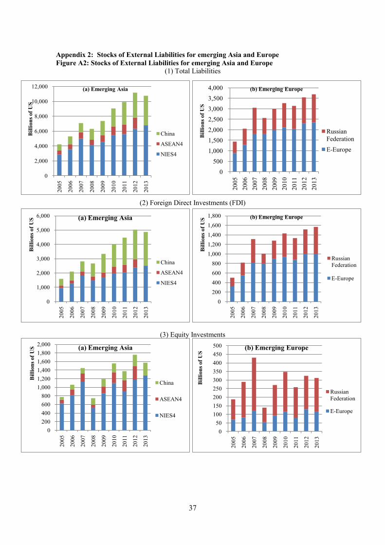
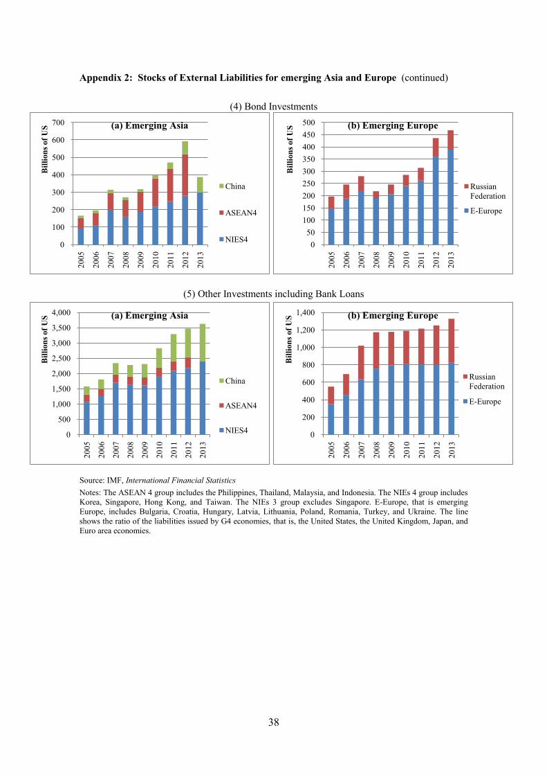
Appendix 2: Stocks of External Liabilities for emerging Asia and Europe

Figure A2: Stocks of External Liabilities for emerging Asia and Europe (1) Total Liabilities

(2) Foreign Direct Investments (FDI)

(3) Equity Investments

38

0

100

200

300

400

500

600

700

20

05

20

06

20

07

20

08

20

09

20

10

20

11

20

12

20

13

Bil

lion

s of

US

(a) Emerging Asia

China

ASEAN4

NIES4 0

50

100

150

200

250

300

350

400

450

500

20

05

20

06

20

07

20

08

20

09

20

10

20

11

20

12

20

13

Bil

lion

s of

US

(b) Emerging Europe

Russian

Federation

E-Europe

0

500

1,000

1,500

2,000

2,500

3,000

3,500

4,000

20

05

20

06

20

07

20

08

20

09

20

10

20

11

20

12

20

13

Bil

lion

s of

US

(a) Emerging Asia

China

ASEAN4

NIES4 0

200

400

600

800

1,000

1,200

1,400

20

05

20

06

20

07

20

08

20

09

20

10

20

11

20

12

20

13

Bil

lion

s of

US

(b) Emerging Europe

Russian

Federation

E-Europe

Appendix 2: Stocks of External Liabilities for emerging Asia and Europe (continued)

(4) Bond Investments

(5) Other Investments including Bank Loans

Source: IMF, International Financial Statistics

Notes: The ASEAN 4 group includes the Philippines, Thailand, Malaysia, and Indonesia. The NIEs 4 group includes

Korea, Singapore, Hong Kong, and Taiwan. The NIEs 3 group excludes Singapore. E-Europe, that is emerging

Europe, includes Bulgaria, Croatia, Hungary, Latvia, Lithuania, Poland, Romania, Turkey, and Ukraine. The line

shows the ratio of the liabilities issued by G4 economies, that is, the United States, the United Kingdom, Japan, and

Euro area economies.

global liquidity and drivers of capital flows to emerging ... · global liquidity and drivers of...

Documents