emissions2Global and regional drivers of accelerating CO

Gernot Klepper, and Christopher B. Field Michael R. Raupach, Gregg Marland, Philippe Ciais, Corinne Le Quéré, Josep G. Canadell,

doi:10.1073/pnas.0700609104 published online May 22, 2007; PNAS

This information is current as of May 2007.

Supplementary Material www.pnas.org/cgi/content/full/0700609104/DC1

Supplementary material can be found at:

www.pnas.org#otherarticlesThis article has been cited by other articles:

E-mail Alerts. click hereat the top right corner of the article or

Receive free email alerts when new articles cite this article - sign up in the box

Rights & Permissions www.pnas.org/misc/rightperm.shtml

To reproduce this article in part (figures, tables) or in entirety, see:

Reprints www.pnas.org/misc/reprints.shtml

To order reprints, see:

Notes:

Global and regional drivers of acceleratingCO2 emissionsMichael R. Raupach*†, Gregg Marland‡, Philippe Ciais§, Corinne Le Quere¶�, Josep G. Canadell*, Gernot Klepper**,and Christopher B. Field††

*Global Carbon Project, Commonwealth Scientific and Industrial Research Organisation, Marine and Atmospheric Research, Canberra, ACT 2601,Australia; ‡Carbon Dioxide Information Analysis Center, Oak Ridge National Laboratory, Oak Ridge, TN 37831; §Commissariat a l’EnergieAtomique, Laboratorie des Sciences du Climat et de l’Environnement, 91191 Gif sur Yvette, France; ¶School of Environment Sciences, University of EastAnglia, Norwich NR4 7TJ United Kingdom; �British Antarctic Survey, Cambridge, CB3 OET, United Kingdom; **Kiel Institute for the World Economy,D- 24105 Kiel, Germany; and ††Carnegie Institution of Washington, Department of Global Ecology, Stanford, CA 94305

Edited by William C. Clark, Harvard University, Cambridge, MA, and approved April 17, 2007 (received for review January 23, 2007)

CO2 emissions from fossil-fuel burning and industrial processeshave been accelerating at a global scale, with their growth rateincreasing from 1.1% y�1 for 1990–1999 to >3% y�1 for 2000–2004. The emissions growth rate since 2000 was greater than forthe most fossil-fuel intensive of the Intergovernmental Panel onClimate Change emissions scenarios developed in the late 1990s.Global emissions growth since 2000 was driven by a cessation orreversal of earlier declining trends in the energy intensity of grossdomestic product (GDP) (energy/GDP) and the carbon intensity ofenergy (emissions/energy), coupled with continuing increases inpopulation and per-capita GDP. Nearly constant or slightly increas-ing trends in the carbon intensity of energy have been recentlyobserved in both developed and developing regions. No region isdecarbonizing its energy supply. The growth rate in emissions isstrongest in rapidly developing economies, particularly China.Together, the developing and least-developed economies (forming80% of the world’s population) accounted for 73% of globalemissions growth in 2004 but only 41% of global emissions andonly 23% of global cumulative emissions since the mid-18th cen-tury. The results have implications for global equity.

carbon intensity of economy � carbon intensity of energy � emissionsscenarios � fossil fuels � Kaya identity

A tmospheric CO2 presently contributes �63% of the gaseousradiative forcing responsible for anthropogenic climate

change (1). The mean global atmospheric CO2 concentration hasincreased from 280 ppm in the 1700s to 380 ppm in 2005, at aprogressively faster rate each decade (2, 3).‡‡ This growth isgoverned by the global budget of atmospheric CO2 (4), whichincludes two major anthropogenic forcing fluxes: (i) CO2 emis-sions from fossil-fuel combustion and industrial processes and(ii) the CO2 flux from land-use change, mainly land clearing. Asurvey of trends in the atmospheric CO2 budget (3) shows thesetwo fluxes were, respectively, 7.9 gigatonnes of carbon (GtC) y�1

and 1.5 GtC y�1 in 2005 with the former growing rapidly overrecent years, and the latter remaining nearly steady.

This paper is focused on CO2 emissions from fossil-fuelcombustion and industrial processes, the dominant anthropo-genic forcing flux. We undertake a regionalized analysis oftrends in emissions and their demographic, economic, andtechnological drivers, using the Kaya identity (defined below)and annual time-series data on national emissions, population,energy consumption, and gross domestic product (GDP). Un-derstanding the observed magnitudes and patterns of the factorsinfluencing global CO2 emissions is a prerequisite for theprediction of future climate and earth system changes and forhuman governance of climate change and the earth system.Although the needs for both understanding and governance havebeen emerging for decades (as demonstrated by the UnitedNations Framework Convention on Climate Change in 1992 andthe Kyoto Protocol in 1997), it is now becoming widely perceivedthat climate change is an urgent challenge requiring globally

concerted action, that a broad portfolio of mitigation measuresis required (5, 6), and that mitigation is not only feasible buthighly desirable on economic as well as social and ecologicalgrounds (7).

The global CO2 emission flux from fossil fuel combustion andindustrial processes (F) includes contributions from sevensources: national-level combustion of solid, liquid, and gaseousfuels; f laring of gas from wells and industrial processes; cementproduction; oxidation of nonfuel hydrocarbons; and fuel from‘‘international bunkers’’ used for shipping and air transport(separated because it is often not included in national invento-ries). Hence

F � FSolid�35%

� FLiquid�36%

� FGas�20%

� FFlare�1%

� FCement�3%

,� FNonFuelHC�1%

� FBunkers�4%

, [1]

where the fractional contribution of each source to the total Ffor 2000–2004 is indicated.

The Kaya identity§§ (8, 9) expresses the global F as a productof four driving factors:

F � P�GP��E

G��FE� � Pgef, [2]

where P is global population, G is world GDP or gross worldproduct, E is global primary energy consumption, g � G/P is theper-capita world GDP, e � E/G is the energy intensity of worldGDP, and f � F/E is the carbon intensity of energy. Upper- andlowercase symbols distinguish extensive and intensive variables,

Author contributions: M.R.R., P.C., C.L.Q., J.G.C., and C.B.F. designed research; M.R.R., G.M.,P.C., and J.G.C. performed research; M.R.R., G.M., P.C., and G.K. analyzed data; and M.R.R.,G.M., G.K., and C.B.F. wrote the paper.

The authors declare no conflict of interest.

This article is a PNAS Direct Submission.

Freely available online through the PNAS open access option.

Abbreviations: GDP, gross domestic product; MER, market exchange rate; PPP, purchasingpower parity; IPCC, Intergovernmental Panel on Climate Change; EU, European Union; FSU,Former Soviet Union; D1, developed countries; D2, developing countries; D3, least-developed countries; CDIAC, U.S. Department of Energy Carbon Dioxide Information andAnalysis Center; EIA, U.S. Department of Energy Energy Information Administration.

†To whom correspondence should be addressed. E-mail: michael.raupach@csiro.au.

‡‡CO2 data are available at www.cmdl.noaa.gov/gmd/ccgg/trends.

§§Yamaji, K., Matsuhashi, R., Nagata, Y., Kaya, Y., An Integrated System for CO2/Energy/GNP Analysis: Case Studies on Economic Measures for CO2 Reduction in Japan. Workshopon CO2 Reduction and Removal: Measures for the Next Century, March 19, 1991,International Institute for Applied Systems Analysis, Laxenburg, Austria.

This article contains supporting information online at www.pnas.org/cgi/content/full/0700609104/DCI.

© 2007 by The National Academy of Sciences of the USA

www.pnas.org�cgi�doi�10.1073�pnas.0700609104 PNAS Early Edition � 1 of 6

SUST

AIN

ABI

LITY

SCIE

NCE

respectively. Combining e and f into the carbon intensity of GDP(h � F/G � ef ), the Kaya identity can also be written as

F � P�GP��F

G� � Pgh. [3]

Defining the proportional growth rate of a quantity X(t) asr(X) � X�1dX/dt (with units [time]�1), the counterpart of theKaya identity for proportional growth rates is

r�F� � r�P� � r� g� � r�e� � r� f � [4]

� r�P� � r� g� � r�h�,

which is an exact, not linearized, result.The world can be disaggregated into regions (distinguished by a

subscript i) with emission Fi, population Pi, GDP Gi, energyconsumption Ei, and regional intensities gi � Gi/Pi, ei � Ei/Gi, fi �Fi/Ei, and hi � Fi/Gi � e i fi. Writing a Kaya identity for each region,the global emission F can be expressed by summation over regionsas:

F � �i

Fi � �i

Pi gi ei fi � �i

Pi gi hi, [5]

and regional contributions to the proportional growth rate inglobal emissions, r(F), are

r�F� � �i

�Fi

F�r�Fi�. [6]

This analysis uses nine noncontiguous regions that span theglobe and cluster nations by their emissions and economicprofiles. The regions comprise four individual nations (U.S.,China, Japan, and India, identified separately because of theirsignificance as emitters); the European Union (EU); the nationsof the Former Soviet Union (FSU); and three regions spanningthe rest of the world, consisting respectively of developed (D1),developing (D2), and least-developed (D3) countries, excludingcountries in other regions.

GDP is defined and measured by using either market exchangerates (MER) or purchasing power parity (PPP), respectively de-noted as GM and GP. The PPP definition gives more weight todeveloping economies. Consequently, wealth disparities are greaterwhen measured by GM than GP, and the growth rate of GP is greaterthan that of GM [supporting information (SI) Fig. 6].

Our measure of Ei is ‘‘commercial’’ primary energy, including(i) fossil fuels, (ii) nuclear, and (iii) renewables (hydro, solar,wind, geothermal, and biomass) when used to generate electric-ity. Total primary energy additionally includes (iv) other energyfrom renewables, mainly as heat from biomass. Contribution ivcan be large in developing regions, but it is not included in Eiexcept in the U.S., where it makes a small (�4%) contribution(SI Text, Primary Energy).

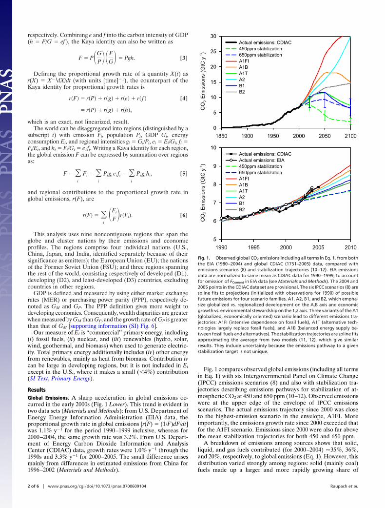
ResultsGlobal Emissions. A sharp acceleration in global emissions oc-curred in the early 2000s (Fig. 1 Lower). This trend is evident intwo data sets (Materials and Methods): from U.S. Department ofEnergy Energy Information Administration (EIA) data, theproportional growth rate in global emissions [r(F) � (1/F)dF/dt]was 1.1% y�1 for the period 1990–1999 inclusive, whereas for2000–2004, the same growth rate was 3.2%. From U.S. Depart-ment of Energy Carbon Dioxide Information and AnalysisCenter (CDIAC) data, growth rates were 1.0% y�1 through the1990s and 3.3% y�1 for 2000–2005. The small difference arisesmainly from differences in estimated emissions from China for1996–2002 (Materials and Methods).

Fig. 1 compares observed global emissions (including all termsin Eq. 1) with six Intergovernmental Panel on Climate Change(IPCC) emissions scenarios (8) and also with stabilization tra-jectories describing emissions pathways for stabilization of at-mospheric CO2 at 450 and 650 ppm (10–12). Observed emissionswere at the upper edge of the envelope of IPCC emissionsscenarios. The actual emissions trajectory since 2000 was closeto the highest-emission scenario in the envelope, A1FI. Moreimportantly, the emissions growth rate since 2000 exceeded thatfor the A1FI scenario. Emissions since 2000 were also far abovethe mean stabilization trajectories for both 450 and 650 ppm.

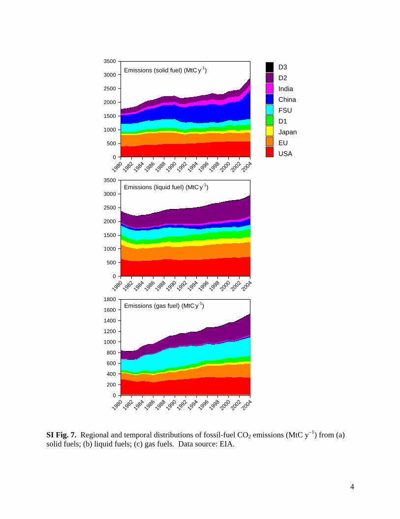
A breakdown of emissions among sources shows that solid,liquid, and gas fuels contributed (for 2000–2004) �35%, 36%,and 20%, respectively, to global emissions (Eq. 1). However, thisdistribution varied strongly among regions: solid (mainly coal)fuels made up a larger and more rapidly growing share of

1990 1995 2000 2005 2010

CO

2 E

mis

sion

s (G

tC y

-1)

5

6

7

8

9

10Actual emissions: CDIACActual emissions: EIA450ppm stabilization650ppm stabilizationA1FI A1B A1T A2 B1 B2

1850 1900 1950 2000 2050 2100

CO

2 E

mis

sion

s (G

tC y

-1)

0

5

10

15

20

25

30Actual emissions: CDIAC450ppm stabilization650ppm stabilizationA1FI A1B A1T A2 B1 B2

Fig. 1. Observed global CO2 emissions including all terms in Eq. 1, from boththe EIA (1980–2004) and global CDIAC (1751–2005) data, compared withemissions scenarios (8) and stabilization trajectories (10–12). EIA emissionsdata are normalized to same mean as CDIAC data for 1990–1999, to accountfor omission of FCement in EIA data (see Materials and Methods). The 2004 and2005 points in the CDIAC data set are provisional. The six IPCC scenarios (8) arespline fits to projections (initialized with observations for 1990) of possiblefuture emissions for four scenario families, A1, A2, B1, and B2, which empha-size globalized vs. regionalized development on the A,B axis and economicgrowth vs. environmental stewardship on the 1,2 axis. Three variants of the A1(globalized, economically oriented) scenario lead to different emissions tra-jectories: A1FI (intensive dependence on fossil fuels), A1T (alternative tech-nologies largely replace fossil fuels), and A1B (balanced energy supply be-tween fossil fuels and alternatives). The stabilization trajectories are spline fitsapproximating the average from two models (11, 12), which give similarresults. They include uncertainty because the emissions pathway to a givenstabilization target is not unique.

2 of 6 � www.pnas.org�cgi�doi�10.1073�pnas.0700609104 Raupach et al.

emissions in developing regions (the sum of China, India, D2,and D3) than in developed regions (U.S., EU, Japan, and D1),and the FSU region had a much stronger reliance on gas than theworld average (SI Fig. 7).

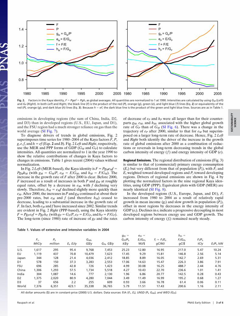
To diagnose drivers of trends in global emissions, Fig. 2superimposes time series for 1980–2004 of the Kaya factors F, P,g, e, f, and h � ef (Eqs. 2 and 3). Fig. 2 Left and Right, respectively,use the MER and PPP forms of GDP (GM and GP) to calculateintensities. All quantities are normalized to 1 in the year 1990 toshow the relative contributions of changes in Kaya factors tochanges in emissions. Table 1 gives recent (2004) values withoutnormalization.

In Fig. 2 Left (MER-based), the Kaya identity is F � PgMeMf �PgMhM (with gM � GM/P, eM � E/GM, and hM � F/GM). Theincrease in the growth rate of F after 2000 is clear. Before 2000,F increased as a result of increases in both P and gM at roughlyequal rates, offset by a decrease in eM, with f declining veryslowly. Therefore, hM � eMf declined slightly more quickly thaneM. After 2000, the increases in P and gM continued at about theirpre-2000 rates, but eM and f (and therefore hM) ceased todecrease, leading to a substantial increase in the growth rate ofF. In fact, both eM and f have increased since 2002. Similar trendsare evident in Fig. 2 Right (PPP-based), using the Kaya identityF � PgP ePf � PgP hP, (with gP � GP/P, eP � E/GP, and hP � F/GP).The long-term (since 1980) rate of increase of gP and the rates

of decrease of eP and hP were all larger than for their counter-parts gM, eM, and hM, associated with the higher global growthrate of GP than of GM (SI Fig. 6). There was a change in thetrajectory of eP after 2000, similar to that for eM but superim-posed on a larger long-term rate of decrease. Hence, Fig. 2 Leftand Right both identify the driver of the increase in the growthrate of global emissions after 2000 as a combination of reduc-tions or reversals in long-term decreasing trends in the globalcarbon intensity of energy ( f ) and energy intensity of GDP (e).

Regional Emissions. The regional distribution of emissions (Fig. 3)is similar to that of (commercial) primary energy consumption(Ei) but very different from that of population (Pi), with Fi andEi weighted toward developed regions and Pi toward developingregions. Drivers of regional emissions are shown in Fig. 4 byplotting the normalized factors in the nine regional Kaya iden-tities, using GDP (PPP). Equivalent plots with GDP (MER) arenearly identical (SI Fig. 8).

In the developed regions (U.S., Europe, Japan, and D1), Fi

increased from 1980 to 2004 as a result of relatively rapidgrowth in mean income (gi) and slow growth in population (Pi),offset in most regions by decreases in the energy intensity ofGDP (ei). Declines in ei indicate a progressive decoupling in mostdeveloped regions between energy use and GDP growth. Thecarbon intensity of energy ( fi) remained nearly steady.

1980 1985 1990 1995 2000 2005

0.8

1.0

1.2

1.4FPgM = GM/P

eM = E/GM

f = F/EhM = F/GM

1980 1985 1990 1995 2000 2005

FPgP = GP/P

eP = E/GP

f = F/EhP = F/GP

Fig. 2. Factors in the Kaya identity, F � Pgef � Pgh, as global averages. All quantities are normalized to 1 at 1990. Intensities are calculated by using GM (Left)and GP (Right). In both Left and Right, the black line (F) is the product of the red (P), orange (g), green (e), and light blue ( f) lines (Eq. 2) or equivalently of thered (P), orange (g), and dark blue (h) lines (Eq. 3). Because h � ef, the dark blue line is the product of the green and light blue lines. Sources are as in Table 1.

Table 1. Values of extensive and intensive variables in 2004

Fi ,MtC/y

Pi,million Ei, EJ/y

GMi,G$/y GPi, G$/y

gPi �

GPi/Pi,k$/y

ePi �

Ei/GPi,MJ/$

fi � Fi/Ei,gC/MJ

hPi �

Fi/GPi,gC/$

Fi/Pi,tC/y Ei/Pi, kW

U.S. 1,617 295 95.4 9,768 7,453 25.23 12.80 16.95 217.0 5.47 10.24EU 1,119 437 70.8 10,479 7,623 17.45 9.29 15.81 146.8 2.56 5.14Japan 344 128 21.4 4,036 2,412 18.85 8.89 16.05 142.7 2.69 5.31D1 578 150 37.3 3,283 2,553 17.06 14.63 15.47 226.3 3.86 7.91FSU 696 285 42.8 726 1,423 4.99 30.08 16.25 488.7 2.44 4.76China 1,306 1,293 57.5 1,734 5,518 4.27 10.43 22.70 236.6 1.01 1.41India 304 1,087 14.6 777 2,130 1.96 6.86 20.77 142.5 0.28 0.43D2 1,375 2,020 80.9 4,280 7,044 3.49 11.49 16.99 195.2 0.68 1.27D3 37 656 2.2 255 609 0.93 3.66 16.78 61.4 0.06 0.11World 7,376 6,351 423.1 35,338 36,765 5.79 11.51 17.43 200.6 1.16 2.11

All dollar amounts ($) are in constant-price (2000) U.S. dollars. Data sources: EIA (Fi , Ei), UNSD (Pi, GMi), and WEO (GPi).

Raupach et al. PNAS Early Edition � 3 of 6

SUST

AIN

ABI

LITY

SCIE

NCE

In the FSU, emissions decreased through the 1990s because ofthe fall in economic activity after the collapse of the SovietUnion. Incomes (gi) decreased in parallel with emissions (Fi),and a shift toward resource-based economic activities led to anincrease in ei and hi. In the late 1990s, incomes started to riseagain, but increases in emissions were slowed by more efficientuse of energy from 2000 on, due to higher prices and shortagesbecause of increasing exports.

In China, gi rose rapidly and Pi slowly over the whole period1980–2004. Progressive decoupling of income growth from energy

consumption (declining ei) was achieved up to �2002, throughimprovements in energy efficiency during the transition to a marketbased economy. Since the early 2000s, there has been a recent rapidgrowth in emissions, associated with very high growth rates inincomes (gi) and a reversal of earlier declines in ei.

In other developing regions (India, D2, and D3), increases inFi were driven by a combination of increases in Pi and gi, with nostrong trends in ei or fi. Growth in emissions (Fi) exceeded growthin income (gi). Unlike China and the developed countries, strongtechnological improvements in energy efficiency have not yetoccurred in these regions, with the exception of India over thelast few years where ei declined.

Differences in intensities across regions are both large (Table1) and persistent in time. There are enormous differences inincome (gi � Gi/Pi), the variation being smaller (although stilllarge) for gPi than for gMi. The energy intensity and carbonintensity of GDP (ei � Ei/Gi and hi � Fi/Gi � ei fi ) varysignificantly between regions, although less than for income (gi).The carbon intensity of energy ( fi � Fi/Ei) varies much less thanother intensities: for most regions, it is between 15 and 20 gramsof carbon per megajoule (gC/MJ), although for China and Indiait is somewhat higher, �20 gC/MJ. In time, fi has decreasedslowly from 1980 to �2000 as a global average (Fig. 2) and inmost regions (Fig. 4). This indicates that the commercial energysupply mix has changed only slowly, even on a regional level. Theglobal average f has increased slightly since 2002.

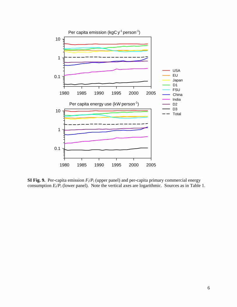
The regional per-capita emissions Fi/Pi � gihi and per-capitaprimary energy consumption Ei/Pi � giei are important indicatorsof global equity. Both quantities vary greatly across regions butmuch less in time (Table 1 and SI Fig. 9). The interregion range,a factor of �50, extends from the U.S. (for which both quantitiesare �5 times the global average) to the D3 region (for which they

CO2 Emissions (MtC y-1)

1980

1982

1984

1986

1988

1990

1992

1994

1996

1998

2000

2002

2004

0

1000

2000

3000

4000

5000

6000

7000

8000

D3

D2

FSUD1

China

India

EU

Japan

USA

Fig. 3. Fossil-fuel CO2 emissions (MtC y�1), for nine regions. Data source isEIA.

FSU

USA

0.5

1.0

1.5

2.0EU

FPg

P = GP/P

eP = E/GP

f = F/Eh

P = F/GP

Japan

D1

0.5

1.0

1.5

2.0China

India

1980 1985 1990 1995 20000.5

1.0

1.5

2.0D2

1980 1985 1990 1995 2000

D3

1980 1985 1990 1995 2000 2005

Fig. 4. Factors in the Kaya identity, F � Pgef � Pgh, for nine regions. All quantities are normalized to 1 at 1990. Intensities are calculated with GPi (PPP). ForFSU, normalizing GPi in 1990 was back-extrapolated. Other details are as for Fig. 2.

4 of 6 � www.pnas.org�cgi�doi�10.1073�pnas.0700609104 Raupach et al.

are �1/10 of the global average). From 1980 to 1999, globalaverage per-capita emissions (F/P � gh) and per-capita primaryenergy consumption (E/P � ge) were both nearly steady at �1.1tC/y per person and 2 kW per person, respectively, but F/P roseby 8% and E/P by 7% over the 5 years 2000–2004.

Temporal Perspectives. In the period 2000–2004, developing coun-tries had a greater share of emissions growth than of emissionsthemselves (Fig. 3). Here we extend this observation by consid-ering cumulative emissions throughout the industrial era (takento start in 1751). The global cumulative fossil-fuel emission C(t)(in gigatonnes of carbon) is defined as the time integral of theglobal emission flux F(t) from 1751 to t. Regional cumulativeemissions Ci(t) are defined similarly.

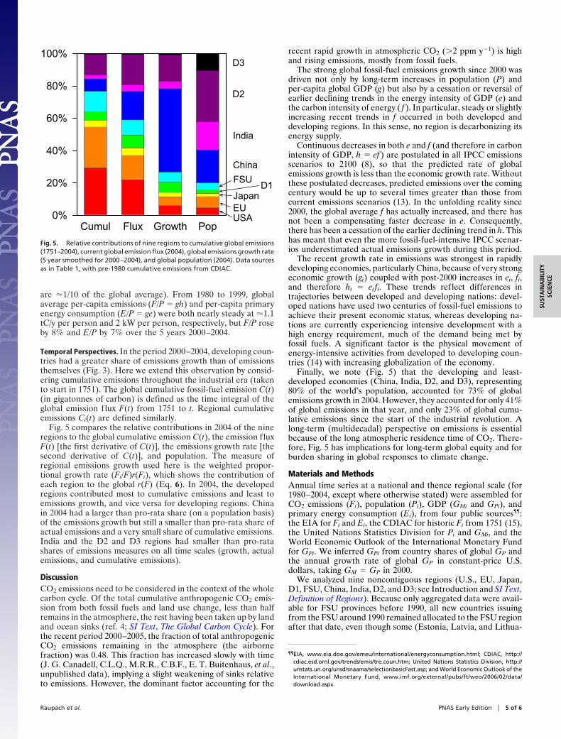
Fig. 5 compares the relative contributions in 2004 of the nineregions to the global cumulative emission C(t), the emission fluxF(t) [the first derivative of C(t)], the emissions growth rate [thesecond derivative of C(t)], and population. The measure ofregional emissions growth used here is the weighted propor-tional growth rate (Fi/F)r(Fi), which shows the contribution ofeach region to the global r(F) (Eq. 6). In 2004, the developedregions contributed most to cumulative emissions and least toemissions growth, and vice versa for developing regions. Chinain 2004 had a larger than pro-rata share (on a population basis)of the emissions growth but still a smaller than pro-rata share ofactual emissions and a very small share of cumulative emissions.India and the D2 and D3 regions had smaller than pro-ratashares of emissions measures on all time scales (growth, actualemissions, and cumulative emissions).

DiscussionCO2 emissions need to be considered in the context of the wholecarbon cycle. Of the total cumulative anthropogenic CO2 emis-sion from both fossil fuels and land use change, less than halfremains in the atmosphere, the rest having been taken up by landand ocean sinks (ref. 4; SI Text, The Global Carbon Cycle). Forthe recent period 2000–2005, the fraction of total anthropogenicCO2 emissions remaining in the atmosphere (the airbornefraction) was 0.48. This fraction has increased slowly with time(J. G. Canadell, C.L.Q., M.R.R., C.B.F., E. T. Buitenhaus, et al.,unpublished data), implying a slight weakening of sinks relativeto emissions. However, the dominant factor accounting for the

recent rapid growth in atmospheric CO2 (�2 ppm y�1) is highand rising emissions, mostly from fossil fuels.

The strong global fossil-fuel emissions growth since 2000 wasdriven not only by long-term increases in population (P) andper-capita global GDP (g) but also by a cessation or reversal ofearlier declining trends in the energy intensity of GDP (e) andthe carbon intensity of energy ( f ). In particular, steady or slightlyincreasing recent trends in f occurred in both developed anddeveloping regions. In this sense, no region is decarbonizing itsenergy supply.

Continuous decreases in both e and f (and therefore in carbonintensity of GDP, h � ef ) are postulated in all IPCC emissionsscenarios to 2100 (8), so that the predicted rate of globalemissions growth is less than the economic growth rate. Withoutthese postulated decreases, predicted emissions over the comingcentury would be up to several times greater than those fromcurrent emissions scenarios (13). In the unfolding reality since2000, the global average f has actually increased, and there hasnot been a compensating faster decrease in e. Consequently,there has been a cessation of the earlier declining trend in h. Thishas meant that even the more fossil-fuel-intensive IPCC scenar-ios underestimated actual emissions growth during this period.

The recent growth rate in emissions was strongest in rapidlydeveloping economies, particularly China, because of very strongeconomic growth (gi) coupled with post-2000 increases in ei, fi,and therefore hi � ei fi. These trends reflect differences intrajectories between developed and developing nations: devel-oped nations have used two centuries of fossil-fuel emissions toachieve their present economic status, whereas developing na-tions are currently experiencing intensive development with ahigh energy requirement, much of the demand being met byfossil fuels. A significant factor is the physical movement ofenergy-intensive activities from developed to developing coun-tries (14) with increasing globalization of the economy.

Finally, we note (Fig. 5) that the developing and least-developed economies (China, India, D2, and D3), representing80% of the world’s population, accounted for 73% of globalemissions growth in 2004. However, they accounted for only 41%of global emissions in that year, and only 23% of global cumu-lative emissions since the start of the industrial revolution. Along-term (multidecadal) perspective on emissions is essentialbecause of the long atmospheric residence time of CO2. There-fore, Fig. 5 has implications for long-term global equity and forburden sharing in global responses to climate change.

Materials and MethodsAnnual time series at a national and thence regional scale (for1980–2004, except where otherwise stated) were assembled forCO2 emissions (Fi), population (Pi), GDP (GMi and GPi), andprimary energy consumption (Ei), from four public sources¶¶:the EIA for Fi and Ei, the CDIAC for historic Fi from 1751 (15),the United Nations Statistics Division for Pi and GMi, and theWorld Economic Outlook of the International Monetary Fundfor GPi. We inferred GPi from country shares of global GP andthe annual growth rate of global GP in constant-price U.S.dollars, taking GM � GP in 2000.

We analyzed nine noncontiguous regions (U.S., EU, Japan,D1, FSU, China, India, D2, and D3; see Introduction and SI Text,Definition of Regions). Because only aggregated data were avail-able for FSU provinces before 1990, all new countries issuingfrom the FSU around 1990 remained allocated to the FSU regionafter that date, even though some (Estonia, Latvia, and Lithua-

¶¶EIA, www.eia.doe.gov/emeu/international/energyconsumption.html; CDIAC, http://cdiac.esd.ornl.gov/trends/emis/tre�coun.htm; United Nations Statistics Division, http://unstats.un.org/unsd/snaama/selectionbasicFast.asp; and World Economic Outlook of theInternational Monetary Fund, www.imf.org/external/pubs/ft/weo/2006/02/data/download.aspx.

Cumul Flux Growth Pop0%

20%

40%

60%

80%

100%D3

India

D2

China

FSUD1

JapanEUUSA

Fig. 5. Relative contributions of nine regions to cumulative global emissions(1751–2004), current global emission flux (2004), global emissions growth rate(5 year smoothed for 2000–2004), and global population (2004). Data sourcesas in Table 1, with pre-1980 cumulative emissions from CDIAC.

Raupach et al. PNAS Early Edition � 5 of 6

SUST

AIN

ABI

LITY

SCIE

NCE

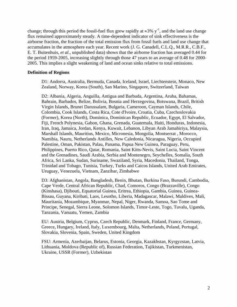
nia) are now members of the EU. European nations who are notmembers of the EU (Norway and Switzerland) were placed ingroup D1. Regions D1 and D3 were defined by using UnitedNations Statistics Division classifications. Region D2 includes allother nations.

Comparisons were made among three different emissionsdata sets: CDIAC global total emissions, CDIAC country-levelemissions, and EIA country-level emissions. These revealedsmall discrepancies with two origins. First, different data setsinclude different components of total emissions, Eq. 1. TheCDIAC global total includes all terms, CDIAC country-leveldata omit FBunkers and FNonFuelHC, and EIA country-level dataomit FCement but include FBunkers by accounting at country ofpurchase. The net effect is that the EIA and CDIAC country-level data yield total emissions (by summation) that are within1% of each other, although they include slightly differentcomponents of Eq. 1, and the CDIAC global total is 4–5%larger than both sums over countries. The second kind of

discrepancy arises from differences at the country level, themain issue being with data for China. Emissions for Chinafrom the EIA and CDIAC data sets both show a significantslowdown in the late 1990s, which is a recognized event (16)associated mainly with closure of small factories and powerplants and with policies to improve energy efficiency (17).However, the CDIAC data suggest a much larger emissionsdecline from 1996 to 2002 than the EIA data (SI Fig. 10). TheCDIAC emissions estimates are based on the UN energy dataset, which is currently undergoing revisions for China. There-fore, we use EIA as the primary source for emissions datasubsequent to 1980.

We thank Mr. Peter Briggs for assistance with preparation of figures.This work has been a collaboration under the Global Carbon Project(GCP, www.globalcarbonproject.org) of the Earth System Science Part-nership (www.essp.org). Support for the GCP from the AustralianClimate Change Science Program is appreciated.

1. Hofmann DJ, Butler JH, Dlugokencky EJ, Elkins JW, Masarie K, Montzka SA,Tans P (2006) Tellus Ser B 58:614–619.

2. Etheridge DM, Steele LP, Langenfelds RL, Francey RJ, Barnola JM, MorganVI (1996) J Geophys Res Atmos 101:4115–4128.

3. Raupach MR, Canadell JG (2007) in Observing the Continental ScaleGreenhouse Gas Balance of Europe, eds Dolman H, Valentini R, FreibauerA (Springer, Berlin), in press.

4. Sabine CL, Heimann M, Artaxo P, Bakker DCE, Chen C-TA, Field CB,Gruber N, Le Quere C, Prinn RG, Richey JD, et al. (2004) in The GlobalCarbon Cycle: Integrating Humans, Climate, and the Natural World, eds FieldCB, Raupach MR (Island, Washington, DC), pp 17–44.

5. Hoffert MI, Caldeira K, Benford G, Criswell DR, Green C, Herzog H, JainAK, Kheshgi HS, Lackner KS, Lewis JS, et al. (2002) Science 298:981–987.

6. Caldeira K, Granger Morgan M, Baldocchi DD, Brewer PG, Chen C-TA,Nabuurs G-J, Nakicenovic N, Robertson GP (2004) in The Global CarbonCycle: Integrating Humans, Climate, and the Natural World, eds Field CB,Raupach MR (Island, Washington, DC), pp 103–129.

7. Stern N (2006) Stern Review on the Economics of Climate Change (CambridgeUniv Press, Cambridge, UK).

8. Nakicenovic N, Alcamo J, Davis G, de Vries B, Fenhann J, Gaffin S, GregoryK, Grubler A, Jung TY, Kram T, et al. (2000) IPCC Special Report on EmissionsScenarios (Cambridge Univ Press, Cambridge, UK).

9. Nakicenovic N (2004) in The Global Carbon Cycle: Integrating Humans, Climate,and the Natural World, eds Field CB, Raupach MR, (Island, Washington, DC),pp 225–239.

10. Houghton JT, Ding Y, Griggs DJ, Noguer M, van der Linden PJ, Dai X,Maskell K, Johnson CA (2001) Climate Change 2001: The Scientific Basis, edsHoughton JT, Ding Y, Griggs DJ, Noguer M, van der Linden PJ, Dai X,Maskell K, Johnson CA (Cambridge Univ Press, Cambridge, UK).

11. Wigley TML, Richels R, Edmonds JA (1996) Nature 379:240–243.12. Joos F, Plattner GK, Stocker TF, Marchal O, Schmittner A (1999) Science

284:464–467.13. Edmonds JA, Joos F, Nakicenovic N, Richels RG, Sarmiento JL (2004) in The

Global Carbon Cycle: Integrating Humans, Climate, and the Natural World, edsField CB, Raupach MR (Island, Washington, DC), pp 77–102.

14. Rothman DS (1998) Ecol Econ 25:177–194.15. Marland G, Rotty RM (1984) Tellus Ser B 36:232–261.16. Streets DG, Jiang KJ, Hu XL, Sinton JE, Zhang XQ, Xu DY, Jacxobson MZ,

Hansen JE (2001) Science 294:1835–1837.17. Wu L, Kaneko S, Matsuoka S (2005) Energy Pol 33:319–335.

6 of 6 � www.pnas.org�cgi�doi�10.1073�pnas.0700609104 Raupach et al.

Global and regional drivers of accelerating CO2 emissions

Michael R. Raupach, Gregg Marland, Philippe Ciais, Corinne Le Quéré, Josep G. Canadell, Gernot Klepper, and Christopher B. Field

PNAS published online May 22, 2007; doi:10.1073/pnas.0700609104

http://www.pnas.org/cgi/reprint/0700609104v1

On-line Supporting Information

SI Text

Primary Energy

Total primary energy consumption includes (i) energy from solid, liquid, and gas fossil fuels; (ii) energy used in nuclear electricity generation; (iii) electricity from renewables (hydroelectric, wind, solar, geothermal, and biomass); and (iv) nonelectrical energy from renewables, mainly as heat from biomass. Commercial primary energy includes contributions i, ii, and iii but excludes iv. Contribution iv can be difficult to measure, especially in developing regions. Its fractional contribution to total primary energy is often large in developing regions (>50%) but is smaller in developed regions. Contribution iv is included in EIA primary-energy data only for the U.S., where it represented a share of total U.S. primary energy of 3.7% (early 1980s) declining to 2.1% (early 2000s). It is not included in the EIA data for regions other than the U.S., so the non-U.S. energy data strictly describe commercial primary energy.

Because of the nature of the energy data, the present analysis applies to commercial primary energy. The presence of contribution iv in energy data for the U.S. introduces a small inconsistency amounting to an overestimate of commercial primary energy for the U.S. averaging ≈3% (declining with time) and an equivalent overestimate of global commercial primary energy averaging ≈0.7% (likewise declining with time).

The intensities ei = Ei/Gi and fi = Fi/Ei are defined for commercial primary energy. Relative to corresponding intensities defined with total primary energy, ei as defined here is an underestimate and fi is an overestimate by the same factor. The carbon intensity of the economy, hi = Fi/Gi = eifi, is independent of the definition of primary energy.

The Global Carbon Cycle

In 2005, the cumulative global fossil-fuel emission of CO2 was C(t) = 319 GtC and the cumulative emission from the other major CO2 source, land use change (J. G. Canadell, C.L.Q., M.R.R., C.B.F., E. T. Buitenhuis, et al., unpublished data) was 156 GtC (3). Of the total cumulative emission from both sources (≈480 GtC), less than half (≈210 GtC) has remained in the atmosphere, the rest having been taken up by land and ocean sinks (4). For the recent period 2000-2005, emission fluxes averaged 7.2 GtC y-1 from fossil fuels and 1.5 GtC y-1 from land use

1

change; through this period the fossil-fuel flux grew rapidly at ≈3% y-1, and the land use change flux remained approximately steady. A time-dependent indicator of sink effectiveness is the airborne fraction, the fraction of the total emission flux from fossil fuels and land use change that accumulates in the atmosphere each year. Recent work (J. G. Canadell, C.L.Q., M.R.R., C.B.F., E. T. Buitenhuis, et al., unpublished data) shows that the airborne fraction has averaged 0.44 for the period 1959-2005, increasing slightly through those 47 years to an average of 0.48 for 2000-2005. This implies a slight weakening of land and ocean sinks relative to total emissions.

Definition of Regions

D1: Andorra, Australia, Bermuda, Canada, Iceland, Israel, Liechtenstein, Monaco, New Zealand, Norway, Korea (South), San Marino, Singapore, Switzerland, Taiwan

D2: Albania, Algeria, Anguilla, Antigua and Barbuda, Argentina, Aruba, Bahamas, Bahrain, Barbados, Belize, Bolivia, Bosnia and Herzegovina, Botswana, Brazil, British Virgin Islands, Brunei Darussalam, Bulgaria, Cameroon, Cayman Islands, Chile, Colombia, Cook Islands, Costa Rica, Cote d'Ivoire, Croatia, Cuba, Czechoslovakia (Former), Korea (North), Dominica, Dominican Republic, Ecuador, Egypt, El Salvador, Fiji, French Polynesia, Gabon, Ghana, Grenada, Guatemala, Haiti, Honduras, Indonesia, Iran, Iraq, Jamaica, Jordan, Kenya, Kuwait, Lebanon, Libyan Arab Jamahiriya, Malaysia, Marshall Islands, Mauritius, Mexico, Micronesia, Mongolia, Montserrat , Morocco, Namibia, Nauru, Netherlands Antilles, New Caledonia, Nicaragua, Nigeria, Occupied Palestine, Oman, Pakistan, Palau, Panama, Papua New Guinea, Paraguay, Peru, Philippines, Puerto Rico, Qatar, Romania, Saint Kitts-Nevis, Saint Lucia, Saint Vincent and the Grenadines, Saudi Arabia, Serbia and Montenegro, Seychelles, Somalia, South Africa, Sri Lanka, Sudan, Suriname, Swaziland, Syria, Macedonia, Thailand, Tonga, Trinidad and Tobago, Tunisia, Turkey, Turks and Caicos Islands, United Arab Emirates, Uruguay, Venezuela, Vietnam, Zanzibar, Zimbabwe

D3: Afghanistan, Angola, Bangladesh, Benin, Bhutan, Burkina Faso, Burundi, Cambodia, Cape Verde, Central African Republic, Chad, Comoros, Congo (Brazzaville), Congo (Kinshasa), Djibouti, Equatorial Guinea, Eritrea, Ethiopia, Gambia, Guinea, Guinea-Bissau, Guyana, Kiribati, Laos, Lesotho, Liberia, Madagascar, Malawi, Maldives, Mali, Mauritania, Mozambique, Myanmar, Nepal, Niger, Rwanda, Samoa, Sao Tome and Principe, Senegal, Sierra Leone, Solomon Islands, Timor-Leste, Togo, Tuvalu, Uganda, Tanzania, Vanuatu, Yemen, Zambia

EU: Austria, Belgium, Cyprus, Czech Republic, Denmark, Finland, France, Germany, Greece, Hungary, Ireland, Italy, Luxembourg, Malta, Netherlands, Poland, Portugal, Slovakia, Slovenia, Spain, Sweden, United Kingdom

FSU: Armenia, Azerbaijan, Belarus, Estonia, Georgia, Kazakhstan, Kyrgyzstan, Latvia, Lithuania, Moldova (Republic of), Russian Federation, Tajikistan, Turkmenistan, Ukraine, USSR (Former), Uzbekistan

2

Energy (EJ y-1)

1980

1982

1984

1986

1988

1990

1992

1994

1996

1998

2000

2002

2004

0

100

200

300

400Population (millions)

1980

1982

1984

1986

1988

1990

1992

1994

1996

1998

2000

2002

2004

0

1000

2000

3000

4000

5000

6000

7000

GDP (MER) (2000 US $b)

1980

1982

1984

1986

1988

1990

1992

1994

1996

1998

2000

2002

2004

0

10000

20000

30000

40000

50000GDP (PPP) (2000 US $b)

1980

1982

1984

1986

1988

1990

1992

1994

1996

1998

2000

2002

2004

0

10000

20000

30000

40000

50000

CO2 Emissions (MtC y-1)

1980

1982

1984

1986

1988

1990

1992

1994

1996

1998

2000

2002

2004

0

1000

2000

3000

4000

5000

6000

7000

8000D3D2IndiaChinaFSUD1JapanEUUSA

SI Fig. 6. Regional and temporal distributions of (a) fossil-fuel CO2 emissions Fi (MtC y−1); (b) commercial energy consumption Ei (EJ y−1); (c) population Pi (millions); (d) GDP (MER) GMi; and (e) GDP (PPP) GPi. GDP is in G$ y−1 (billions of constant-price 2000 US dollars per year). Sources as in Table 1.

3

Emissions (liquid fuel) (MtC y-1)

1980

1982

1984

1986

1988

1990

1992

1994

1996

1998

2000

2002

2004

0

500

1000

1500

2000

2500

3000

3500

Emissions (gas fuel) (MtC y-1)

1980

1982

1984

1986

1988

1990

1992

1994

1996

1998

2000

2002

2004

0

200

400

600

800

1000

1200

1400

1600

1800

Emissions (solid fuel) (MtC y-1)

1980

1982

1984

1986

1988

1990

1992

1994

1996

1998

2000

2002

2004

0

500

1000

1500

2000

2500

3000

3500D3D2IndiaChinaFSUD1JapanEUUSA

SI Fig. 7. Regional and temporal distributions of fossil-fuel CO2 emissions (MtC y−1) from (a) solid fuels; (b) liquid fuels; (c) gas fuels. Data source: EIA.

4

FSU

USA

0.5

1.0

1.5

2.0EU

FPgM = GM/PeM = E/GM

f = F/EhM = F/GM

Japan

D1

0.5

1.0

1.5

2.0China

India

1980 1985 1990 1995 20000.5

1.0

1.5

2.0D2

1980 1985 1990 1995 2000

D3

1980 1985 1990 1995 2000 2005

SI Fig. 8. Factors in the Kaya identity, F = Pgef = Pgh, for nine regions. All quantities are normalised to 1 at 1990. Intensities are calculated with GMi (MER). Other details as for Figure 2.

5

Per capita emission (kgC y-1 person-1)

1980 1985 1990 1995 2000 2005

0.1

1

10

USA EU Japan D1 FSU China India D2 D3 Total

Per capita energy use (kW person-1)

1980 1985 1990 1995 2000 2005

0.1

1

10

SI Fig. 9. Per-capita emission Fi/Pi (upper panel) and per-capita primary commercial energy consumption Ei/Pi (lower panel). Note the vertical axes are logarithmic. Sources as in Table 1.

6

1980 1985 1990 1995 2000 20053000

4000

5000

6000

7000

8000

9000

EIA (sum)CDIAC (sum)CDIAC (global)

Global CO2 emissions (MtC y-1)

1980 1985 1990 1995 2000 20050

200

400

600

800

1000

1200

1400

EIA (sum)CDIAC (sum)

China CO2 emissions (MtC y-1)

SI Fig. 10. (Upper panel) Observed CO2 emissions: from EIA data summed over all countries (red), from CDIAC data summed over all countries (green), and the global total from the CDIAC dataset (blue). (Lower panel) Emissions from China, from EIA (red) and CDIAC (blue) data.

7