geotechnical characterization of a highway route …2fs40703-015-0007-2.pdf · original research...
TRANSCRIPT
Ilori International Journal of Geo-Engineering (2015) 6:7 DOI 10.1186/s40703-015-0007-2
ORIGINAL RESEARCH Open Access
Geotechnical characterization of a highwayroute alignment with light weight penetrometer(LRS 10), in southeastern NigeriaAbidemi O. Ilori
Correspondence:[email protected],[email protected] of Civil Engineering,University of Uyo, Uyo, Akwa-IbomState, Nigeria
©LmC
Abstract
Background: It is required to carry out geotechnical characterization of the subgradefor a proposed 18 km dual carriageway alignment. A light weight penetrometer, LRS 10was chosen as an exploratory tool to carry out the investigation.
Methods: The LRS 10 penetrometer was deployed at an average interval of 250 malong the proposed alignment, and was used to sound the soil consistency up to 6.0 mdepth. Trial pits were dug at locations closed to the LRS 10 sounding positions fromwhich soil samples were collected for laboratory analysis. A software, UK DCP version 3.1was employed to analyze the LRS 10 field data.
Results: The LRS 10 results classified the highway alignment into three zones basedon in situ relative density while the UK DCP software gives penetration index and CBRvalues of soil layers from the ground surface up to 1.5m depth. Laboratory analysesplaces the dominant soils in the area into clayey sand (SC, A-2- 4, A-2- 6), silty sand(SM, A-2-7), and a combination of the two (SM-SC, A-6). Exception is the occurrenceof Inorganic silt MH and ML, and organic silt OH (A-7-5) in a few locations along thealignment. These soils are predominantly nonexpansive (plasticity index less than 15 %)but a few are moderately expansive (plasticity index between 15 and 25 %). Sub-gradestiffness as indicated by resilient modulus values were estimated from the largestpenetration index values (lowest strength) using established correlation equations; thisgives resilient modulus values between 27 MPa to 304 MPa.
Conclusion: The soil types dominant along the proposed highway alignment wereclassified and characterized in strength. The soil types is consistent with the geology ofthe area the alignment transects. The subgrade stiffness of some sections of thealignment will need improvement to meet minimum strength required for a highwaypavement. Some useful correlations of strength parameters were proposed.
Keywords: Quaternary; Southeastern Nigeria; German LRS 10; Penetration index;Resilient modulus; Young’s modulus
IntroductionThe highway that links the states of Abia and Akwa-Ibom in southeastern part of
Nigeria is at present a two-lane, two-way carriage way. The road is presently in a bad
state with many failures in more than eighty percent of its total length of 34 km. The
road has significant economic importance due to the fact that it also serves as the only
gateway from the southern end of the country into Cross River state, the state
2015 Ilori. Open Access This article is distributed under the terms of the Creative Commons Attribution 4.0 Internationalicense (http://creativecommons.org/licenses/by/4.0/), which permits unrestricted use, distribution, and reproduction in anyedium, provided you give appropriate credit to the original author(s) and the source, provide a link to the Creativeommons license, and indicate if changes were made.
Ilori International Journal of Geo-Engineering (2015) 6:7 Page 2 of 28
bounding Akwa-Ibom at its Northern end. The highway, therefore, is critical to move-
ment of goods and persons between the three states and to the remaining part of the
country. The first 16 km. of the highway is presently being reconstructed into a dual
carriage way. This paper presents the geotechnical characterization of alignment pro-
posed for the remaining 18 km.
Objectives
The objectives of the geotechnical characterization are:
1. Identify soil domains in the proposed alignment and their extent in width and
depth along the alignment.
2. Determine engineering properties of the soil domains based both on field and
laboratory tests.
3. The influence of the engineering properties of the soil domains to the proposed
construction and eventual behavior of the highway pavement.
Site description and geology of the study area
The proposed dualisation alignment follows the existing road in most part. The existing
alignment is crossed by two seasonal streams with associated bridges. The geotechnical
characterization at these two bridge sites crossing the two rivers are excluded from this
investigation. Generally, the alignment has flat topography with no undulations except at
the seasonal stream sites where approaches are characterized with valleys. The geographical
co-ordinates of the alignment termini are 05° 07′ 9.9″ N, 07′ 22" 17.52″ E for Aba, and
05° 08′ 28.9″ N, 07° 33′ 34.99″ E for Ikot-Umo Essien.
According to the Nigerian Geological Survey Agency 2006 base map of Akwa–Ibom State,
the geology of the area spans from Cretaceous through Tertiary to Quaternary. In the
Cretaceous, the following in younger succession characterize the area. These are the Asu River
Group, Eze Aku Shale Group, Lower Coal Measures, False Bedded Sandstones and Upper Coal
Measures. In the Tertiary also, in younger succession, the Imo Shale Group, Bende Ameki
Group, Coastal Plain Sands, and Alluvium constitute the Formations within the study area. The
surficial geology along the alignment in general is the clastic sediments of Coastal Plain Sands
and the Lignite Series Formations which have ages in the range between Tertiary to early
Quaternary. Lithology essentially is sands and clay in the former, and lignite, claystone and shale
in the latter Formation. These two formations form the youngest stratigraphic units in the area.
Penetrometers
Different types of penetrometers are in use for foundation investigation and characterization,
the most common being the Dutch Cone Penetrometer (CPT) and Standard Penetrometer
(SPT- ASTM D-1586 2011). Advances in geotechnical instrumentation have seen many
improvements in both penetrometers, but more have been made on the Dutch Cone
Penetrometer (CPT) than the SPT. The CPT has seen improvements and developments that
increase its capability to handle differing ground conditions (Campanella et al. 1982), and
accurately identify soil types (Begemann 1965, Olsen and Farr 1986; Robertson 1990), and
give better estimates of relevant geotechnical soil parameters. For geotechnical
characterization of a highway, the SPT is a bulky equipment to deploy. Although depth of
investigation could be 30 m or more, which is far higher than what is usually required for a
Ilori International Journal of Geo-Engineering (2015) 6:7 Page 3 of 28
highway pavement (FHWA NHI–05–037 2006), The depth of investigation is based on zone
of influence, which for the asphalt pavement is about 3.81 m (Vandre et al. 1998). The result
obtained with SPT is usually bearing stress or bearing capacity. The same is true for the CPT,
although it is easier to deploy the CPT, than the SPT. Both of them are capable of deep inves-
tigation which comes into play in that part of a highway that needs embankment fillings, or
at potential bridge sites. For highway geotechnical investigations other types of portable and
light weight penetrometers are available which include the Dynamic Cone Penetrometer
(DCP) developed by (Sowers and Hedges, 1966), and the German Light weight Penetrome-
ters (LRS5, LRS 10 – DIN 4094 Part 2). The LRS 10 Penetrometer was used in this study
to characterize the soil condition on highway alignment. Both the DCP and LRS 10 are
easy to deploy and dismantle. In its original form the DCP consists of 6.8 kg steel mass
falling through a height of 50.8 cm that strikes the anvil to cause penetration of a 3.8 cm
diameter 45° vertex angle cone that has been seated in the bottom of a hand-augered hole.
The blows required to drive the embedded cone to a depth of 450 mm have been corre-
lated by others to N values derived from the Standard Penetration Test (SPT). Experience
has shown that the DCP can be used effectively in augered holes to depths of 4.0 m to
6.0 m. In performing the tests a cumulative number of blows over the depth of penetra-
tion are recorded. There have been variations of the DCP in terms of hammer weight; an
8 kg hammer is sometimes used. The DCP is often used to evaluate or characterize pave-
ments. It is also used to characterize the sub-grade.
The LRS 10 penetrometer
The LRS 10 is equipped with an anvil and driving rod, a 10 kg rammer, rammer fall of
50 cm, 11 sounding rods, lifting device for sounding rods, and couplings all in a box cas-
ing weighing approximately 71 kg. If soil to be investigated is not in the dense to very
dense consistencies penetration test can be carried out to between 10 to 12 m. The tip
cone can either be 45° or 60°. The cone tip angle of the penetrometer used in this study is
the 60°. The rods are 20.0 mm in diameter. The LRS 10 acquires data in the number of
blows per 10 cm penetration. DIN 4094 Part 2, (1980) gives guidance on both qualitative
and quantitative interpretation of the LRS 10 readings. Qualitative interpretation factors
that influence the LRS 10 reistance pattern when used in predominantly sandy soil ac-
cording to “DIN4094” include skin friction, overburden and depth, ground water, and in-
fluence of layer limit. For quantitave interpretation, “DIN 4094” gives an equation that
estimates relative densities of diffrent soil strata in situ. The equation is of the form
ID ¼0:21þ0:230 log n10 ð1Þ
where n10 is the number of blows per 10 cm. Compared to the SPT, the LRS 10 probes
10 cm thickness of soil at a time versus 30.5 cm for the SPT. It can therefore detect
changes in soil consistency within shorter reaches than the SPT.
Site investigation
Penetration test
The proposed alignment partly follows the existing road. The road has an unpaved
shoulder. The penetrations tests were carried out 4.0 to 5.0 m after the edge of the
existing pavement. Overburden materials consisting of vegetative materials with humus
Ilori International Journal of Geo-Engineering (2015) 6:7 Page 4 of 28
were first removed until a uniform soil color was encountered or exposed. The thickness
of these overburden materials varies from about 0.150 m to about 0.40 m. After the re-
moval of the overburden, the LRS 10 was set up and used to probe the soil consistencies
with depth along the proposed alignment. The Penetrometer tests were located at intervals
of 250 m on either side of the alignment, alternately in most cases of the tests, but other-
wise at some locations. Depth of investigation was 5.0 m to 6.0 m. The test points are des-
ignated serially starting from Test No. 1 to Test No. 55. Test no. 1 was located at
21.650 km, while Test No. 55 at 36.400 km, 00 + 000 km being a mileage post in Uyo City
representing the origin of the distances along the alignment. These tests were performed
during the month of March, before the full onset of the rainy season.
Soil sample collection
Disturbed soil samples were collected from trial pits dug along the alignment. They
were dug to a depth of 3.0 m and are located close to the points where penetration
tests were carried out. Samples were collected all along the depths as there were no
visible changes in soil types or lithology.
Laboratory analysis
Samples of soil collected at different trial pit locations and depths were tested for index prop-
erties. Other tests carried out on them include: Moisture- Density relationship test using
West African compaction test (modified Proctor Type A-ASTM-D1557), and California
Bearing Ratio test. All tests were performed in accordance with relevant ASTM standards.
Results and discussionSoil indices, classification, and physical properties
Sieve Analysis
Sieve analysis results for some of the soil samples are presented in Table 1 which shows soil
indices and basic properties of all the sampled locations. The results showed that for most of
the soil sampled, the percentage passing sieve no. 200 is less than 50 %, with values ranging
between 23.8 % at 22.65 km to 45.6 % at 33.25 km, placing most of the soil in the coarse
grained texture. Exception to this trend are soils sampled from kilometers 26.85, 27.25, 34.75,
and 35.00 along the alignment where the percentages passing no. 200 sieve are 57, 58.2, 54.8,
and 56.4 % respectively. Some grain size analysis results are presented in Fig. 1.
Atterberg limits
Some Atterberg Limits results are also presented in Table 1. Liquid Limit values ranged
from 30.0 to 55.9 %, while Plastic Limits values are between 16.9 and 36.6 %. Plasticity
Index values range from a minimum 8.2 % to a maximum value of 24.3 %, indicating
low to moderately swelling potential as presented in Fig. 2 which is a modified
Casagrande plasticity chart. This also shows plots of soil domains.
Soil classification
Soil laboratory analyses results of Atterberg Limits with sieve analysis places the soil in-
vestigated in quite a wide range of soil types. Based on the American Association of
State Highways and Transportation Officials (AASHTO) soil classification systems soil
along the proposed alignment includes A–2–4, A–2–6, A–2–7, A–7–5, A–7–6, and
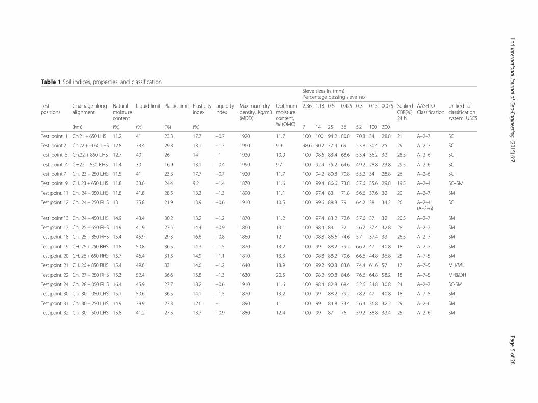
Table 1 Soil indices, properties, and classification
Sieve sizes in (mm)Percentage passing sieve no
Testpositions
Chainage alongalignment
Naturalmoisturecontent
Liquid limit Plastic limit Plasticityindex
Liquidityindex
Maximum drydensity, Kg/m3(MDD)
Optimummoisturecontent,% (OMC)
2.36 1.18 0.6 0.425 0.3 0.15 0.075 SoakedCBR(%)24 h
AASHTOClassification
Unified soilclassificationsystem, USCS
(km) (%) (%) (%) (%) 7 14 25 36 52 100 200
Test point. 1 Ch.21 + 650 LHS 11.2 41 23.3 17.7 −0.7 1920 11.7 100 100 94.2 80.8 70.8 34 28.8 21 A–2–7 SC
Test point.2 Ch.22 +−050 LHS 12.8 33.4 29.3 13.1 −1.3 1960 9.9 98.6 90.2 77.4 69 53.8 30.4 25 29 A–2–7 SC
Test point. 5 Ch.22 + 850 LHS 12.7 40 26 14 −1 1920 10.9 100 98.6 83.4 68.6 53.4 36.2 32 28.5 A–2–6 SC
Test point. 4 CH22 + 650 RHS 11.4 30 16.9 13.1 −0.4 1990 9.7 100 92.4 75.2 64.6 49.2 28.8 23.8 29.5 A–2–6 SC
Test point.7 Ch.. 23 + 250 LHS 11.5 41 23.3 17.7 −0.7 1920 11.7 100 94.2 80.8 70.8 55.2 34 28.8 26 A–2–6 SC
Test point. 9 CH. 23 + 650 LHS 11.8 33.6 24.4 9.2 −1.4 1870 11.6 100 99.4 86.6 73.8 57.6 35.6 29.8 19.5 A–2–4 SC–SM
Test point. 11 Ch.. 24 + 050 LHS 11.8 41.8 28.5 13.3 −1.3 1890 11.1 100 97.4 83 71.8 56.6 37.6 32 20 A–2–7 SM
Test point. 12 Ch.. 24 + 250 RHS 13 35.8 21.9 13.9 −0.6 1910 10.5 100 99.6 88.8 79 64.2 38 34.2 26 A–2–4(A–2–6)
SC
Test point.13 Ch.. 24 + 450 LHS 14.9 43.4 30.2 13.2 −1.2 1870 11.2 100 97.4 83.2 72.6 57.6 37 32 20.5 A–2–7 SM
Test point. 17 Ch.. 25 + 650 RHS 14.9 41.9 27.5 14.4 −0.9 1860 13.1 100 98.4 83 72 56.2 37.4 32.8 28 A–2–7 SM
Test point. 18 Ch.. 25 + 850 RHS 15.4 45.9 29.3 16.6 −0.8 1860 12 100 98.8 86.6 74.6 57 37.4 33 26.5 A–2–7 SM
Test point. 19 CH. 26 + 250 RHS 14.8 50.8 36.5 14.3 −1.5 1870 13.2 100 99 88.2 79.2 66.2 47 40.8 18 A–2–7 SM
Test point. 20 CH. 26 + 650 RHS 15.7 46.4 31.5 14.9 −1.1 1810 13.3 100 98.8 88.2 79.6 66.6 44.8 36.8 25 A–7–5 SM
Test point. 21 CH. 26 + 850 RHS 15.4 49.6 33 14.6 −1.2 1640 18.9 100 99.2 90.8 83.6 74.4 61.6 57 17 A–7–5 MH/ML
Test point. 22 Ch.. 27 + 250 RHS 15.3 52.4 36.6 15.8 −1.3 1630 20.5 100 98.2 90.8 84.6 76.6 64.8 58.2 18 A–7–5 MH&OH
Test point. 24 Ch.. 28 + 050 RHS 16.4 45.9 27.7 18.2 −0.6 1910 11.6 100 98.4 82.8 68.4 52.6 34.8 30.8 24 A–2–7 SC-SM
Test point. 30 Ch.. 30 + 050 LHS 15.1 50.6 36.5 14.1 −1.5 1870 13.2 100 99 88.2 79.2 78.2 47 40.8 18 A–7–5 SM
Test point. 31 Ch.. 30 + 250 LHS 14.9 39.9 27.3 12.6 −1 1890 11 100 99 84.8 73.4 56.4 36.8 32.2 29 A–2–6 SM
Test point. 32 Ch.. 30 + 500 LHS 15.8 41.2 27.5 13.7 −0.9 1880 12.4 100 99 87 76 59.2 38.8 33.4 25 A–2–6 SM
IloriInternationalJournalofGeo-Engineering
(2015) 6:7 Page
5of
28
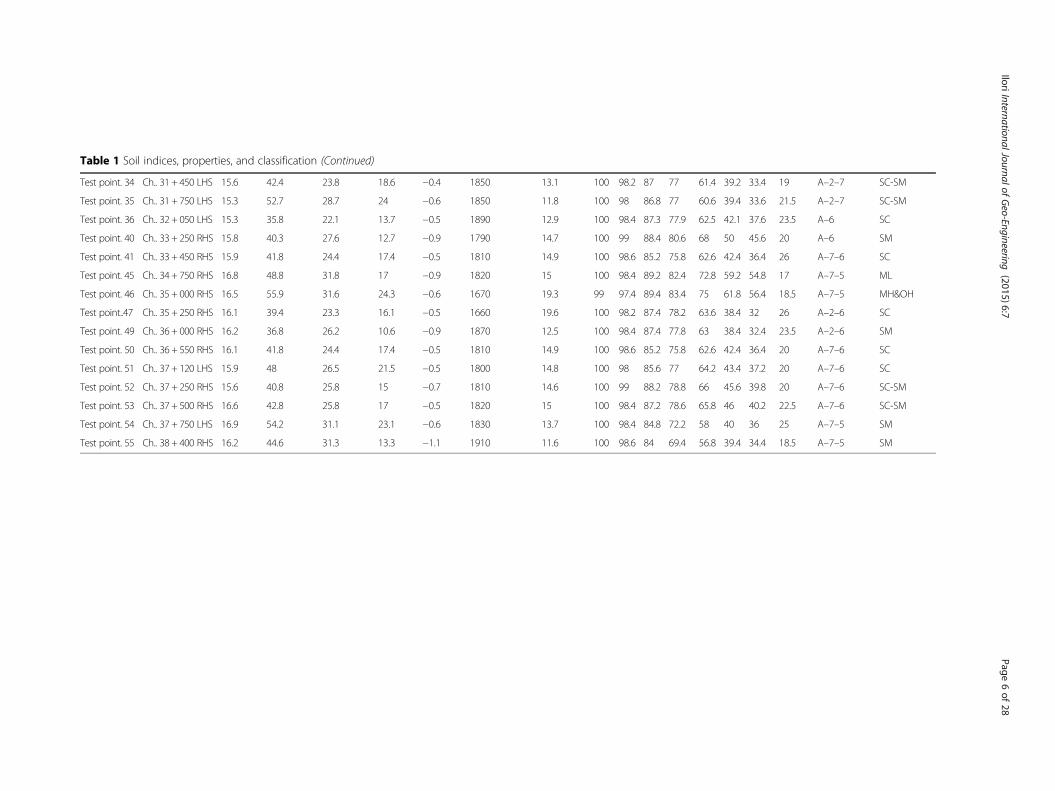
Table 1 Soil indices, properties, and classification (Continued)
Test point. 34 Ch.. 31 + 450 LHS 15.6 42.4 23.8 18.6 −0.4 1850 13.1 100 98.2 87 77 61.4 39.2 33.4 19 A–2–7 SC-SM
Test point. 35 Ch.. 31 + 750 LHS 15.3 52.7 28.7 24 −0.6 1850 11.8 100 98 86.8 77 60.6 39.4 33.6 21.5 A–2–7 SC-SM
Test point. 36 Ch.. 32 + 050 LHS 15.3 35.8 22.1 13.7 −0.5 1890 12.9 100 98.4 87.3 77.9 62.5 42.1 37.6 23.5 A–6 SC
Test point. 40 Ch.. 33 + 250 RHS 15.8 40.3 27.6 12.7 −0.9 1790 14.7 100 99 88.4 80.6 68 50 45.6 20 A–6 SM
Test point. 41 Ch.. 33 + 450 RHS 15.9 41.8 24.4 17.4 −0.5 1810 14.9 100 98.6 85.2 75.8 62.6 42.4 36.4 26 A–7–6 SC
Test point. 45 Ch.. 34 + 750 RHS 16.8 48.8 31.8 17 −0.9 1820 15 100 98.4 89.2 82.4 72.8 59.2 54.8 17 A–7–5 ML
Test point. 46 Ch.. 35 + 000 RHS 16.5 55.9 31.6 24.3 −0.6 1670 19.3 99 97.4 89.4 83.4 75 61.8 56.4 18.5 A–7–5 MH&OH
Test point..47 Ch.. 35 + 250 RHS 16.1 39.4 23.3 16.1 −0.5 1660 19.6 100 98.2 87.4 78.2 63.6 38.4 32 26 A–2–6 SC
Test point. 49 Ch.. 36 + 000 RHS 16.2 36.8 26.2 10.6 −0.9 1870 12.5 100 98.4 87.4 77.8 63 38.4 32.4 23.5 A–2–6 SM
Test point. 50 Ch.. 36 + 550 RHS 16.1 41.8 24.4 17.4 −0.5 1810 14.9 100 98.6 85.2 75.8 62.6 42.4 36.4 20 A–7–6 SC
Test point. 51 Ch.. 37 + 120 LHS 15.9 48 26.5 21.5 −0.5 1800 14.8 100 98 85.6 77 64.2 43.4 37.2 20 A–7–6 SC
Test point. 52 Ch.. 37 + 250 RHS 15.6 40.8 25.8 15 −0.7 1810 14.6 100 99 88.2 78.8 66 45.6 39.8 20 A–7–6 SC-SM
Test point. 53 Ch.. 37 + 500 RHS 16.6 42.8 25.8 17 −0.5 1820 15 100 98.4 87.2 78.6 65.8 46 40.2 22.5 A–7–6 SC-SM
Test point. 54 Ch.. 37 + 750 LHS 16.9 54.2 31.1 23.1 −0.6 1830 13.7 100 98.4 84.8 72.2 58 40 36 25 A–7–5 SM
Test point. 55 Ch.. 38 + 400 RHS 16.2 44.6 31.3 13.3 −1.1 1910 11.6 100 98.6 84 69.4 56.8 39.4 34.4 18.5 A–7–5 SM
IloriInternationalJournalofGeo-Engineering
(2015) 6:7 Page
6of
28
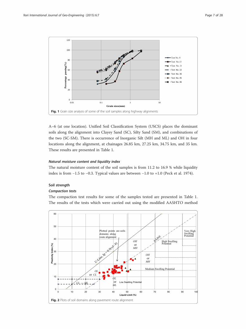
Fig. 1 Grain size analysis of some of the soil samples along highway alignments
Ilori International Journal of Geo-Engineering (2015) 6:7 Page 7 of 28
A–6 (at one location). Unified Soil Classification System (USCS) places the dominant
soils along the alignment into Clayey Sand (SC), Silty Sand (SM), and combinations of
the two (SC-SM). There is occurrence of Inorganic Silt (MH and ML) and OH in four
locations along the alignment, at chainages 26.85 km, 27.25 km, 34.75 km, and 35 km.
These results are presented in Table 1.
Natural moisture content and liquidity index
The natural moisture content of the soil samples is from 11.2 to 16.9 % while liquidity
index is from −1.5 to −0.3. Typical values are between −1.0 to +1.0 (Peck et al. 1974).
Soil strength
Compaction tests
The compaction test results for some of the samples tested are presented in Table 1.
The results of the tests which were carried out using the modified AASHTO method
Fig. 2 Plots of soil domains along pavement route alignment
Ilori International Journal of Geo-Engineering (2015) 6:7 Page 8 of 28
showed that the value for Maximum Dry Density (MDD) for soil ranges from
1630.0 kg/m3 at distance 27.25 km to 1990 kg/m3 at 22.65 km; and the optimum mois-
ture content (OMC) ranges from 9.4 to 20.5 % at 22.45 km and 27.25 km respectively.
Laboratory California bearing ratio test
California Bearing Ratio (CBR) values range from 15.5 % at location 33.05 km to 29.5 %
at 22.65 km . Test points with liquidity index values of −1.2 and below have exception-
ally low values of CBR. These samples were collected at distances 23.65, 24.05, 24.45,
26.25, 26.65, 26.85, 27.25, 30.05 and 38.40 kilometers along the alignment route. Excep-
tions to this trend are soils at locations 22.05 km and 25.45 km with a CBR value of
29 %. All the locations listed with Liquidity Index values of −1.2 and below have CBR
values between 15 and 20.5 % representing values that are the lowest in the CBR range
of values. These soils are mostly SM, SC-SM, ML, OH, and MH types. Soil in these lo-
cations are said to be sensitive, that is, they lose strength when disturbed. Das (1983).
Some of these results are presented in Table 1. Physically the soil samples collected are
fine to medium grain, dark yellowish in color and semi-solid in consistency.
Ground water
Static ground water table was not encountered in any of the trial pits dug for the col-
lection of soil samples throughout the length of the alignment.
Penetration resistance, penetration index, and relative density
The LRS 10 Penetrometer used for the penetration tests have similar dimensions of the
critical parts, and the operation is similar to the Dynamic Cone Penetrometer (DCP).
The main difference is the size of the hammer which is slightly heavier in LRS 10, being
10 kg. While the standard DCP delivers 45.472 Joules of energy with a hammer of 8 kg
falling through 575 mm, the LRS 10 delivers 49 Joules falling through 500 mm, result-
ing in a difference in energy of 3.528 Joules. This translates to the estimation of Pene-
tration Index values (the key parameter in penetrometer analysis) in error of about
7.75 % (3.528/45.472) on the conservative side.
The LRS 10 readings for the first 1.50 m are therefore interpreted like DCP readings.
The interpretation was carried out using the UK DCP software version 3.1 (Done and
Samuel 2006). The software analyzes the LRS 10 readings and identifies layers of differ-
ent strengths as measured by Penetration Index and lists the CBR values for each layer
and the depth of each layer from the ground surface. The program output is a chart
that shows a plot of these identified layers. A Typical chart is displayed in Fig. 3. The
software plots cumulative numbers of blows versus depth, and identifies layers based
on points falling on the same straight line where the slope is different from the next
straight line joining another set of points. The slope of such line of locus is the Penetra-
tion Index. The software uses an equation that relates Penetration Index with CBR.
The equation was proposed by Transport and Road Research Laboratory (1990), and is
given as
Log10 CBRð Þ ¼ 2:48−1:057Log10 penrateð Þ ð2Þ
Where
pen rate = penetration index.
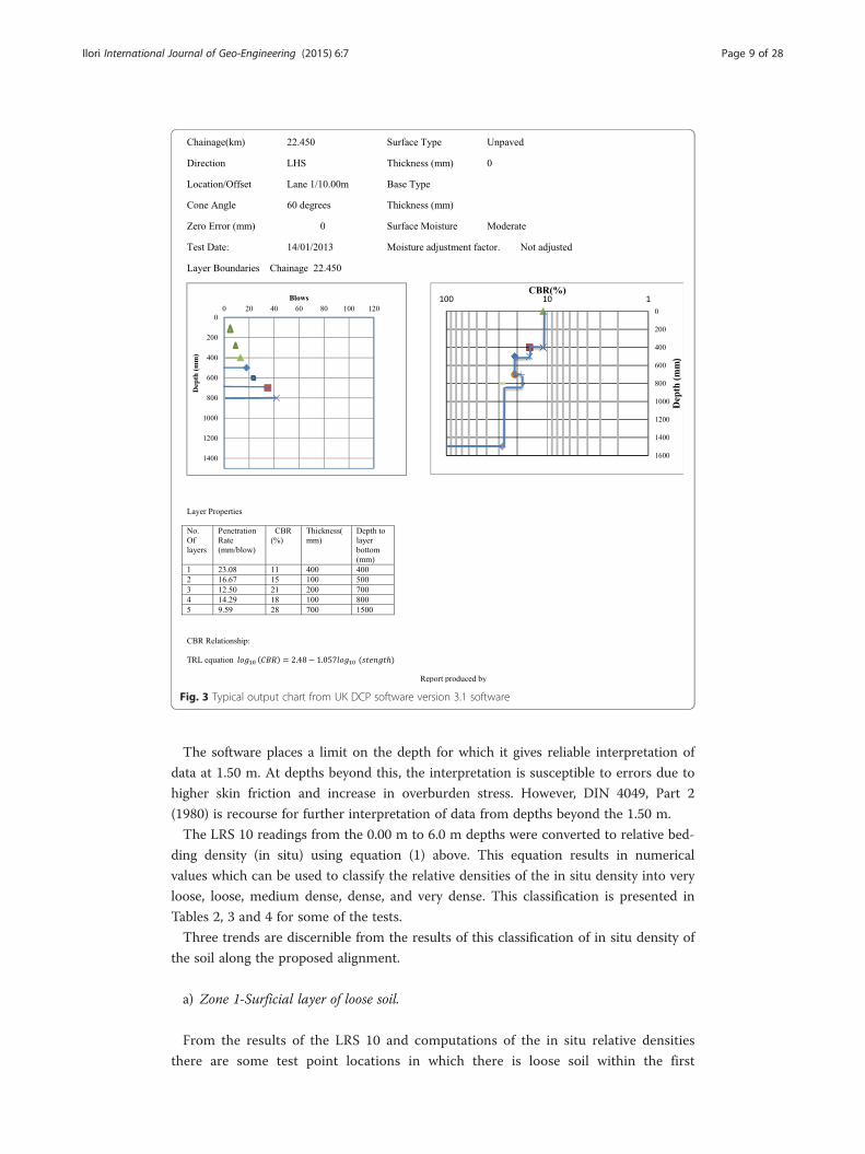
Fig. 3 Typical output chart from UK DCP software version 3.1 software
Ilori International Journal of Geo-Engineering (2015) 6:7 Page 9 of 28
The software places a limit on the depth for which it gives reliable interpretation of
data at 1.50 m. At depths beyond this, the interpretation is susceptible to errors due to
higher skin friction and increase in overburden stress. However, DIN 4049, Part 2
(1980) is recourse for further interpretation of data from depths beyond the 1.50 m.
The LRS 10 readings from the 0.00 m to 6.0 m depths were converted to relative bed-
ding density (in situ) using equation (1) above. This equation results in numerical
values which can be used to classify the relative densities of the in situ density into very
loose, loose, medium dense, dense, and very dense. This classification is presented in
Tables 2, 3 and 4 for some of the tests.
Three trends are discernible from the results of this classification of in situ density of
the soil along the proposed alignment.
a) Zone 1-Surficial layer of loose soil.
From the results of the LRS 10 and computations of the in situ relative densities
there are some test point locations in which there is loose soil within the first
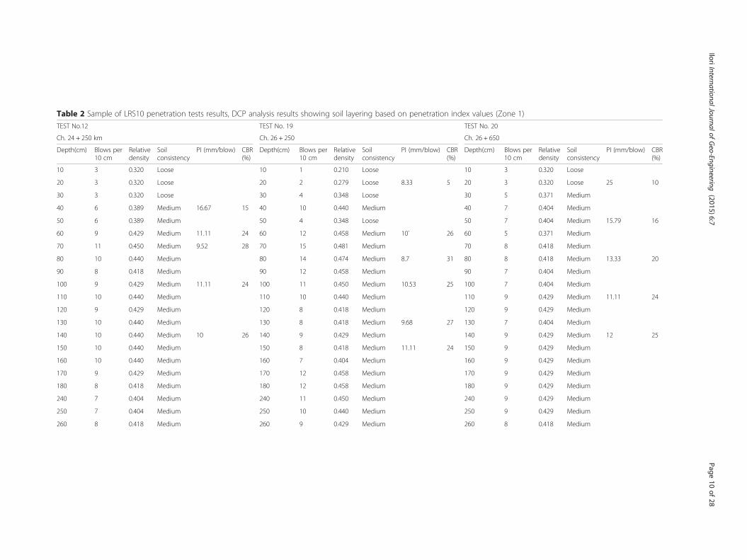
Table 2 Sample of LRS10 penetration tests results, DCP analysis results showing soil layering based on penetration index values (Zone 1)
TEST No.12 TEST No. 19 TEST No. 20
Ch. 24 + 250 km Ch. 26 + 250 Ch. 26 + 650
Depth(cm) Blows per10 cm
Relativedensity
Soilconsistency
PI (mm/blow) CBR(%)
Depth(cm) Blows per10 cm
Relativedensity
Soilconsistency
PI (mm/blow) CBR(%)
Depth(cm) Blows per10 cm
Relativedensity
Soilconsistency
PI (mm/blow) CBR(%)
10 3 0.320 Loose 10 1 0.210 Loose 10 3 0.320 Loose
20 3 0.320 Loose 20 2 0.279 Loose 8.33 5 20 3 0.320 Loose 25 10
30 3 0.320 Loose 30 4 0.348 Loose 30 5 0.371 Medium
40 6 0.389 Medium 16.67 15 40 10 0.440 Medium 40 7 0.404 Medium
50 6 0.389 Medium 50 4 0.348 Loose 50 7 0.404 Medium 15.79 16
60 9 0.429 Medium 11.11 24 60 12 0.458 Medium 10` 26 60 5 0.371 Medium
70 11 0.450 Medium 9.52 28 70 15 0.481 Medium 70 8 0.418 Medium
80 10 0.440 Medium 80 14 0.474 Medium 8.7 31 80 8 0.418 Medium 13.33 20
90 8 0.418 Medium 90 12 0.458 Medium 90 7 0.404 Medium
100 9 0.429 Medium 11.11 24 100 11 0.450 Medium 10.53 25 100 7 0.404 Medium
110 10 0.440 Medium 110 10 0.440 Medium 110 9 0.429 Medium 11.11 24
120 9 0.429 Medium 120 8 0.418 Medium 120 9 0.429 Medium
130 10 0.440 Medium 130 8 0.418 Medium 9.68 27 130 7 0.404 Medium
140 10 0.440 Medium 10 26 140 9 0.429 Medium 140 9 0.429 Medium 12 25
150 10 0.440 Medium 150 8 0.418 Medium 11.11 24 150 9 0.429 Medium
160 10 0.440 Medium 160 7 0.404 Medium 160 9 0.429 Medium
170 9 0.429 Medium 170 12 0.458 Medium 170 9 0.429 Medium
180 8 0.418 Medium 180 12 0.458 Medium 180 9 0.429 Medium
240 7 0.404 Medium 240 11 0.450 Medium 240 9 0.429 Medium
250 7 0.404 Medium 250 10 0.440 Medium 250 9 0.429 Medium
260 8 0.418 Medium 260 9 0.429 Medium 260 8 0.418 Medium
IloriInternationalJournalofGeo-Engineering
(2015) 6:7 Page
10of
28
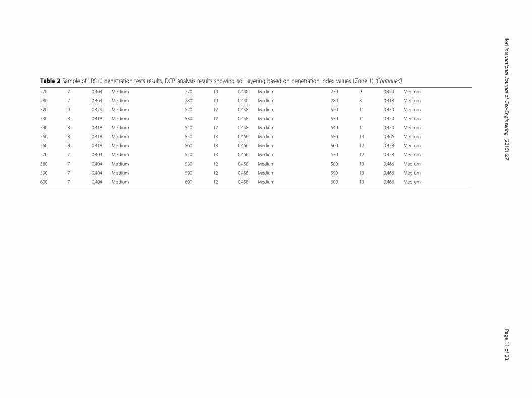
Table 2 Sample of LRS10 penetration tests results, DCP analysis results showing soil layering based on penetration index values (Zone 1) (Continued)
270 7 0.404 Medium 270 10 0.440 Medium 270 9 0.429 Medium
280 7 0.404 Medium 280 10 0.440 Medium 280 8 0.418 Medium
520 9 0.429 Medium 520 12 0.458 Medium 520 11 0.450 Medium
530 8 0.418 Medium 530 12 0.458 Medium 530 11 0.450 Medium
540 8 0.418 Medium 540 12 0.458 Medium 540 11 0.450 Medium
550 8 0.418 Medium 550 13 0.466 Medium 550 13 0.466 Medium
560 8 0.418 Medium 560 13 0.466 Medium 560 12 0.458 Medium
570 7 0.404 Medium 570 13 0.466 Medium 570 12 0.458 Medium
580 7 0.404 Medium 580 12 0.458 Medium 580 13 0.466 Medium
590 7 0.404 Medium 590 12 0.458 Medium 590 13 0.466 Medium
600 7 0.404 Medium 600 12 0.458 Medium 600 13 0.466 Medium
IloriInternationalJournalofGeo-Engineering
(2015) 6:7 Page
11of
28
Table 3 Sample of LRS10 penetration tests results, DCP analysis results showing soil layering based on penetration index values (Zone 2)
TEST no. 2 TEST No.10 TEST No.25
CH22+ 050 LHS CH. 23 + 850 RHS CH. 28 + 450 RHS .
Depth (cm) Blows per10 cm
Relativedensity
Soilconsistency
PI (mm/blow) CBR(%)
Depth (cm) Blows per10 cm
Relativedensity
Soilconsistency
PI (mm/blow) CBR(%)
Depth (cm) Blows per10 cm
Relativedensity
Soilconsistency
PI (mm/blow) CBR(%)
10 9 0.429 Medium 16 14.27 10 5 0.371 Medium 10 4 0.348 Loose
20 7 0.404 Medium 20 10 0.440 Medium 11.76 22 20 5 0.371 Medium
30 3 0.320 Loose 30 7 0.404 Medium 30 5 0.371 Medium 22.73 11
40 3 0.320 Loose 30.77 8 40 3 0.320 Loose 40 3 0.320 Loose
50 4 0.348 Loose 50 3 0.320 Loose 27.76 9 50 4 0.348 Loose
60 3 0.320 Loose 60 4 0.348 Loose 60 3 0.320 Loose
70 4 0.348 Loose 25 10 70 4 0.348 Loose 70 3 0.320 Loose 20 13
80 5 0.371 Medium 80 4 0.348 Loose 80 2 0.279 Loose 16.67 15
90 4 0.348 Loose 90 3 0.320 Loose 33.33 7 90 3 0.320 Loose
100 4 0.348 Loose 22.73 11 100 3 0.320 Loose 100 3 0.320 Loose
110 4 0.348 Loose 110 3 0.320 Loose 110 3 0.320 Loose 13.16 20
120 5 0.371 Medium 120 4 0.348 Loose 120 3 0.320 Loose
130 4 0.348 Loose 25 10 130 6 0.389 Medium 20 13 130 3 0.320 Loose
140 4 0.348 Loose 140 5 0.371 Medium 140 2 0.279 Loose 16.67 15
150 4 0.348 Loose 150 3 0.320 Loose 33.33 7 150 2 0.279 Loose
160 4 0.348 Loose 160 3 0.320 Loose 160 2 0.279 Loose
170 4 0.348 Loose 170 4 0.348 Loose 170 3 0.320 Loose
180 5 0.371 Medium 180 4 0.348 Loose 180 3 0.320 Loose
190 5 0.371 Medium 190 5 0.371 Medium 190 2 0.279 Loose
200 6 0.389 Medium 200 5 0.371 Medium 200 3 0.320 Loose
210 7 0.404 Medium 210 4 0.348 Loose 210 3 0.320 Loose
IloriInternationalJournalofGeo-Engineering
(2015) 6:7 Page
12of
28
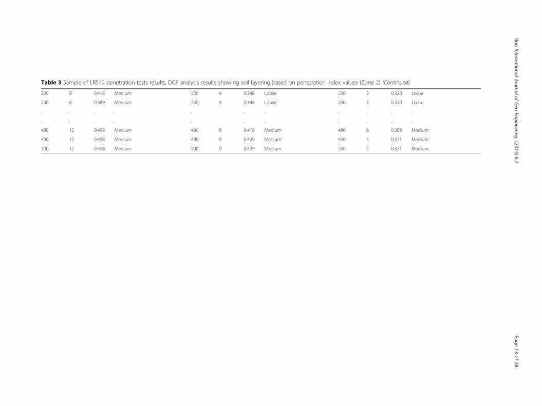
Table 3 Sample of LRS10 penetration tests results, DCP analysis results showing soil layering based on penetration index values (Zone 2) (Continued)
220 8 0.418 Medium 220 4 0.348 Loose 220 3 0.320 Loose
230 6 0.389 Medium 230 4 0.348 Loose 230 3 0.320 Loose
. . . . . . . . . . .
. . . . . . . . . . .
480 12 0.458 Medium 480 8 0.418 Medium 480 6 0.389 Medium
490 12 0.458 Medium 490 9 0.429 Medium 490 5 0.371 Medium
500 12 0.458 Medium 500 9 0.429 Medium 500 5 0.371 Medium
IloriInternationalJournalofGeo-Engineering
(2015) 6:7 Page
13of
28
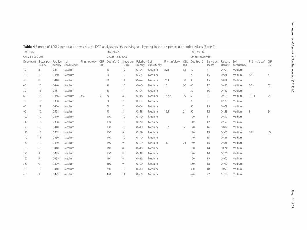
Table 4 Sample of LRS10 penetration tests results, DCP analysis results showing soil layering based on penetration index values (Zone 3)
TEST no.7 TEST No.24 TEST No. 49
CH. 23 + 250 LHS CH. 28 + 050 RHS CH 36 + 000 RHS
Depth(cm) Blows per10 cm
Relativedensity
Soilconsistency
PI (mm/blow) CBR(%)
Depth(cm) Blows per10 cm
Relativedensity
Soilconsistency
PI (mm/blow) CBR(%)
Depth(cm) Blows per10 cm
Relativedensity
Soilconsistency
PI (mm/blow) CBR(%)
10 5 0.371 Medium 10 19 0.504 Medium 5.26 52 10 7 0.404 Medium
20 10 0.440 Medium 20 19 0.504 Medium 20 15 0.481 Medium 6.67 41
30 8 0.418 Medium 30 14 0.474 Medium 7.14 38 30 15 0.481 Medium
40 10 0.440 Medium 40 10 0.440 Medium 10 26 40 12 0.458 Medium 8.33 32
50 15 0.481 Medium 50 7 0.404 Medium 50 10 0.440 Medium
60 13 0.466 Medium 8.92 30 60 8 0.418 Medium 13.79 19 60 8 0.418 Medium 11.11 24
70 12 0.458 Medium 70 7 0.404 Medium 70 9 0.429 Medium
80 12 0.458 Medium 80 7 0.404 Medium 80 15 0.481 Medium
90 12 0.458 Medium 90 8 0.418 Medium 12.5 21 90 12 0.458 Medium 8 34
100 10 0.440 Medium 100 10 0.440 Medium 100 11 0.450 Medium
110 12 0.458 Medium 110 10 0.440 Medium 110 12 0.458 Medium
120 10 0.440 Medium 120 10 0.440 Medium 10.2 26 120 16 0.487 Medium
130 12 0.458 Medium 130 9 0.429 Medium 130 13 0.466 Medium 6.78 40
140 11 0.450 Medium 140 10 0.440 Medium 140 15 0.481 Medium
150 10 0.440 Medium 150 9 0.429 Medium 11.11 24 150 15 0.481 Medium
160 10 0.440 Medium 160 8 0.418 Medium 160 14 0.474 Medium
170 9 0.429 Medium 170 8 0.418 Medium 170 14 0.474 Medium
180 9 0.429 Medium 180 8 0.418 Medium 180 13 0.466 Medium
380 9 0.429 Medium 380 9 0.429 Medium 380 18 0.499 Medium
390 10 0.440 Medium 390 10 0.440 Medium 390 18 0.499 Medium
470 9 0.429 Medium 470 11 0.450 Medium 470 22 0.519 Medium
IloriInternationalJournalofGeo-Engineering
(2015) 6:7 Page
14of
28
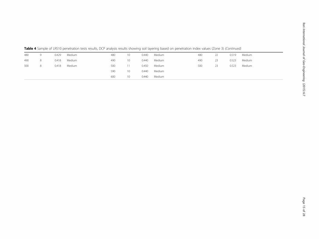
Table 4 Sample of LRS10 penetration tests results, DCP analysis results showing soil layering based on penetration index values (Zone 3) (Continued)
480 9 0.429 Medium 480 10 0.440 Medium 480 22 0.519 Medium
490 8 0.418 Medium 490 10 0.440 Medium 490 23 0.523 Medium
500 8 0.418 Medium 500 11 0.450 Medium 500 23 0.523 Medium
590 10 0.440 Medium
600 10 0.440 Medium
IloriInternationalJournalofGeo-Engineering
(2015) 6:7 Page
15of
28
Ilori International Journal of Geo-Engineering (2015) 6:7 Page 16 of 28
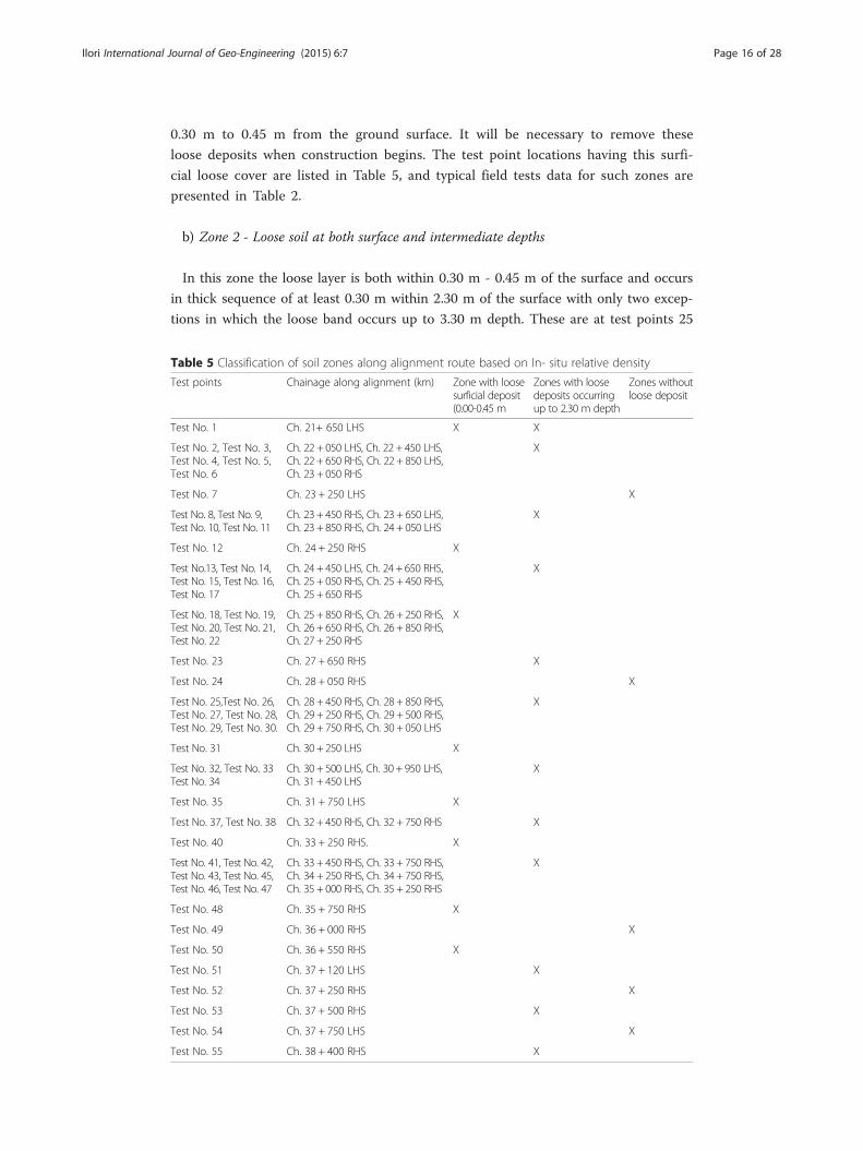
0.30 m to 0.45 m from the ground surface. It will be necessary to remove these
loose deposits when construction begins. The test point locations having this surfi-
cial loose cover are listed in Table 5, and typical field tests data for such zones are
presented in Table 2.
b) Zone 2 - Loose soil at both surface and intermediate depths
In this zone the loose layer is both within 0.30 m - 0.45 m of the surface and occurs
in thick sequence of at least 0.30 m within 2.30 m of the surface with only two excep-
tions in which the loose band occurs up to 3.30 m depth. These are at test points 25
Table 5 Classification of soil zones along alignment route based on In- situ relative density
Test points Chainage along alignment (km) Zone with loosesurficial deposit(0.00-0.45 m
Zones with loosedeposits occurringup to 2.30 m depth
Zones withoutloose deposit
Test No. 1 Ch. 21+ 650 LHS X X
Test No. 2, Test No. 3,Test No. 4, Test No. 5,Test No. 6
Ch. 22 + 050 LHS, Ch. 22 + 450 LHS,Ch. 22 + 650 RHS, Ch. 22 + 850 LHS,Ch. 23 + 050 RHS
X
Test No. 7 Ch. 23 + 250 LHS X
Test No. 8, Test No. 9,Test No. 10, Test No. 11
Ch. 23 + 450 RHS, Ch. 23 + 650 LHS,Ch. 23 + 850 RHS, Ch. 24 + 050 LHS
X
Test No. 12 Ch. 24 + 250 RHS X
Test No.13, Test No. 14,Test No. 15, Test No. 16,Test No. 17
Ch. 24 + 450 LHS, Ch. 24 + 650 RHS,Ch. 25 + 050 RHS, Ch. 25 + 450 RHS,Ch. 25 + 650 RHS
X
Test No. 18, Test No. 19,Test No. 20, Test No. 21,Test No. 22
Ch. 25 + 850 RHS, Ch. 26 + 250 RHS,Ch. 26 + 650 RHS, Ch. 26 + 850 RHS,Ch. 27 + 250 RHS
X
Test No. 23 Ch. 27 + 650 RHS X
Test No. 24 Ch. 28 + 050 RHS X
Test No. 25,Test No. 26,Test No. 27, Test No. 28,Test No. 29, Test No. 30.
Ch. 28 + 450 RHS, Ch. 28 + 850 RHS,Ch. 29 + 250 RHS, Ch. 29 + 500 RHS,Ch. 29 + 750 RHS, Ch. 30 + 050 LHS
X
Test No. 31 Ch. 30 + 250 LHS X
Test No. 32, Test No. 33Test No. 34
Ch. 30 + 500 LHS, Ch. 30 + 950 LHS,Ch. 31 + 450 LHS
X
Test No. 35 Ch. 31 + 750 LHS X
Test No. 37, Test No. 38 Ch. 32 + 450 RHS, Ch. 32 + 750 RHS X
Test No. 40 Ch. 33 + 250 RHS. X
Test No. 41, Test No. 42,Test No. 43, Test No. 45,Test No. 46, Test No. 47
Ch. 33 + 450 RHS, Ch. 33 + 750 RHS,Ch. 34 + 250 RHS, Ch. 34 + 750 RHS,Ch. 35 + 000 RHS, Ch. 35 + 250 RHS
X
Test No. 48 Ch. 35 + 750 RHS X
Test No. 49 Ch. 36 + 000 RHS X
Test No. 50 Ch. 36 + 550 RHS X
Test No. 51 Ch. 37 + 120 LHS X
Test No. 52 Ch. 37 + 250 RHS X
Test No. 53 Ch. 37 + 500 RHS X
Test No. 54 Ch. 37 + 750 LHS X
Test No. 55 Ch. 38 + 400 RHS X
Ilori International Journal of Geo-Engineering (2015) 6:7 Page 17 of 28
(28.450 km) and 47 (35.250 km). These bands of loose soil occur to within 2.90 m
depth at test points 43 (34.250 km) and 51 (37.120 km).
Test point locations characterized with this trend of loose band of soil are listed in
Table 5. This zone is the most dominant.
c) Zone 3 - Loose soil completely absent
These locations do not have loose soil present at all, both at the surface and at depth.
Test locations with such characteristics are listed in Table 5, and Table 4 presents samples
of such test locations.
The loose soil in zones 1 and 2 within 0.0 m to 0.45 m of the existing ground
surface can be removed as part of ground stripping and removal of vegetative
layer. However, beyond 0.45 m depth there is need to increase the density of the
soil up to 2.90 m depth. This can be achieved by compaction of the soil with
impact or polygonal compactor machines. These machines have compactive effort
effect that can penetrate depth up to 2.10 m or more (Kloubert 2009; Jaksa et al.
2012), and will consolidate the soil up to the required depth and thereby
strengthen the soil.
Correlations
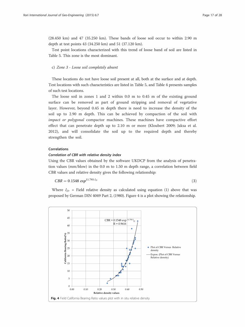
Correlation of CBR with relative density index
Using the CBR values obtained by the software UKDCP from the analysis of penetra-
tion values (mm/blow) in the 0.0 m to 1.50 m depth range, a correlation between field
CBR values and relative density gives the following relationship:
CBR ¼ 0:1548 exp11:793 ID ð3Þ
Where ID. = Field relative density as calculated using equation (1) above that was
proposed by German DIN 4049 Part 2, (1980). Figure 4 is a plot showing the relationship.
Fig. 4 Field California Bearing Ratio values plot with in situ relative density
Ilori International Journal of Geo-Engineering (2015) 6:7 Page 18 of 28
The values of relative densities used in obtaining equation 3 above are from loose
(0.255) to medium range (0.476)). There was no value in the dense or very dense re-
gion. According to DIN 4049, Part 2 (1980), the maximum In situ relative density that
can be sounded by LRS 10 is 0.5 in soil in which the ground water table is not
encountered during exploration, and approximately 0.55 where ground water is
encountered.
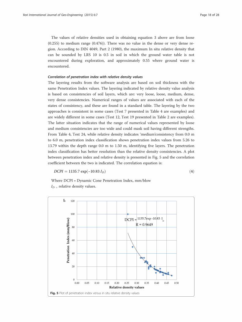
Correlation of penetration index with relative density values
The layering results from the software analysis are based on soil thickness with the
same Penetration Index values. The layering indicated by relative density value analysis
is based on consistencies of soil layers, which are: very loose, loose, medium, dense,
very dense consistencies. Numerical ranges of values are associated with each of the
states of consistency, and these are found in a standard table. The layering by the two
approaches is consistent in some cases (Test 7 presented in Table 4 are examples) and
are widely different in some cases (Test 12, Test 19 presented in Table 2 are examples).
The latter situation indicates that the range of numerical values represented by loose
and medium consistencies are too wide and could mask soil having different strengths.
From Table 4, Test 24, while relative density indicates ‘medium’consistency from 0.0 m
to 6.0 m, penetration index classification shows penetration index values from 5.26 to
13.79 within the depth range 0.0 m to 1.50 m, identifying five layers. The penetration
index classification has better resolution than the relative density consistencies. A plot
between penetration index and relative density is presented in Fig. 5 and the correlation
coefficient between the two is indicated. The correlation equation is:
DCPI ¼ 1135:7 exp −10:83 IDð Þ ð4Þ
Where DCPI = Dynamic Cone Penetration Index, mm/blow
ID = relative density values.
Fig. 5 Plot of penetration index versus in situ relative density values
Ilori International Journal of Geo-Engineering (2015) 6:7 Page 19 of 28
Subgrade stiffness-resilient and Young’s modulus estimation
The Resilient Modulus (MR) is a measure of sub-grade material stiffness. A material’s
resilient modulus is an estimate of its modulus of elasticity (E). While the modulus of
elasticity is stress divided by strain for a slowly applied load, resilient modulus is stress
divided by strain for rapidly applied loads (Pavement interactive, 2007). During a resili-
ent modulus test, a very “small” permanent strain accompanies each load cycle; this is
absent in Elastic modulus test (Irwin 2009). The laboratory determination of resilient
modulus is quite involved, hence other methods of estimating its value from other soil
properties that can be readily determined was explored.
A number of relationships are available in literature on the estimation of resilient
modulus using the Penetration Index of the DCP and CBR laboratory data. For DCP,
Pen (1990); De Beer and van der Merwe (1991); Lockwood et al. (1992); Lee et al.
(1997a); George and Uddin (2000); and Chen et al. (2005), all gave relationships that
allow estimation of resilient modulus from Penetration Index values. Some specified
the type of soil (coarse or fine grained); the expression is applicable to. The values of
resilient modulus for the test point locations obtained with expressions proposed by
Lockwood et al. (1992); Lee et al. (1997b); and George and Uddin (2000), are presented
in Tables 6 and 7. The equations utilized are:
MR ¼ 103:04758−1:06166 log DCPI½ � ð5Þ
By Lockwood et al.(1992), for any type of soil.
MR ¼ −3279DCPIþ 114100 ð6Þ
By Lee et al. (1997a), for fine grained soil and,
MR ¼ 235:3� DCPI−0:475 ð7Þ
by George and Uddin (2000), for coarse grained soil.
in these relationships,
MR = Resilient Modulus in kPa in equation (1), and MPa in equations (6) and (7)
DCPI = Dynamic Cone Penetration Test Index.
The Penetration Index values used were from the results of DCP software analysis
which analyses the DCP data from zero to 1.5 m depth. A further refinement of the re-
sult was made by using the highest value of Penetration Index (lowest strength) ob-
tained in the range of 0.30 m to 1.50 m depth for each test location. The top 0.30 m
were excluded since this may likely be removed during earthworks stripping
operations.
Values of resilient modulus obtained by the three expressions for DCPI values of
30 mm/blow and above, (30.7 mm/blow, 33.33 mm/blow, 50 mm/blow and 100 mm/
blow) correlates poorly. There are wide differences in values of the MR computed by
these expressions. Test positions that have this trend are Test Nos. 2, 6, 10, 25, 28, 29,
30, 33, 34, 38, 43, 46, & 53. The values at these test locations are presented in Table 7.
For DCPI values below 30 mm/blow the difference in resilient modulus values between
the lowest and the highest values obtained by all of these methods, in most cases,
is not more than 10 MPa. The results are presented in Table 6. Exceptions to this
are values with DCPI of 25 mm/blow and 26.67 mm/blow. The values for these
exceptions are not as widely dispersed as the values for those with DCPI of
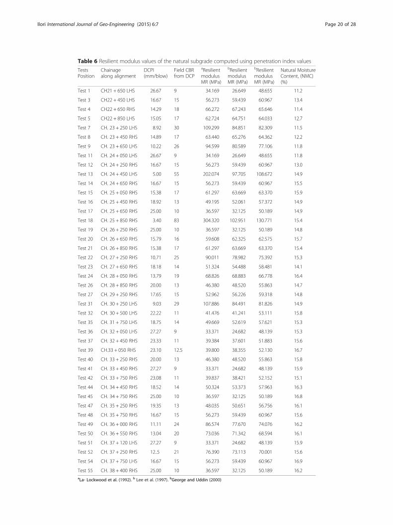
Table 6 Resilient modulus values of the natural subgrade computed using penetration index values
TestsPosition
Chainagealong alignment
DCPI(mm/blow)
Field CBRfrom DCP
aResilientmodulusMR (MPa)
bResilientmodulusMR (MPa)
bResilientmodulusMR (MPa)
Natural MoistureContent, (NMC)(%)
Test 1 CH21 + 650 LHS 26.67 9 34.169 26.649 48.655 11.2
Test 3 CH22 + 450 LHS 16.67 15 56.273 59.439 60.967 13.4
Test 4 CH22 + 650 RHS 14.29 18 66.272 67.243 65.646 11.4
Test 5 CH22 + 850 LHS 15.05 17 62.724 64.751 64.033 12.7
Test 7 CH. 23 + 250 LHS 8.92 30 109.299 84.851 82.309 11.5
Test 8 CH. 23 + 450 RHS 14.89 17 63.440 65.276 64.362 12.2
Test 9 CH. 23 + 650 LHS 10.22 26 94.599 80.589 77.106 11.8
Test 11 CH. 24 + 050 LHS 26.67 9 34.169 26.649 48.655 11.8
Test 12 CH. 24 + 250 RHS 16.67 15 56.273 59.439 60.967 13.0
Test 13 CH. 24 + 450 LHS 5.00 55 202.074 97.705 108.672 14.9
Test 14 CH. 24 + 650 RHS 16.67 15 56.273 59.439 60.967 15.5
Test 15 CH. 25 + 050 RHS 15.38 17 61.297 63.669 63.370 15.9
Test 16 CH. 25 + 450 RHS 18.92 13 49.195 52.061 57.372 14.9
Test 17 CH. 25 + 650 RHS 25.00 10 36.597 32.125 50.189 14.9
Test 18 CH. 25 + 850 RHS 3.40 83 304.320 102.951 130.771 15.4
Test 19 CH. 26 + 250 RHS 25.00 10 36.597 32.125 50.189 14.8
Test 20 CH. 26 + 650 RHS 15.79 16 59.608 62.325 62.575 15.7
Test 21 CH. 26 + 850 RHS 15.38 17 61.297 63.669 63.370 15.4
Test 22 CH. 27 + 250 RHS 10.71 25 90.011 78.982 75.392 15.3
Test 23 CH. 27 + 650 RHS 18.18 14 51.324 54.488 58.481 14.1
Test 24 CH. 28 + 050 RHS 13.79 19 68.826 68.883 66.778 16.4
Test 26 CH. 28 + 850 RHS 20.00 13 46.380 48.520 55.863 14.7
Test 27 CH. 29 + 250 RHS 17.65 15 52.962 56.226 59.318 14.8
Test 31 CH. 30 + 250 LHS 9.03 29 107.886 84.491 81.826 14.9
Test 32 CH. 30 + 500 LHS 22.22 11 41.476 41.241 53.111 15.8
Test 35 CH. 31 + 750 LHS 18.75 14 49.669 52.619 57.621 15.3
Test 36 CH. 32 + 050 LHS 27.27 9 33.371 24.682 48.139 15.3
Test 37 CH. 32 + 450 RHS 23.33 11 39.384 37.601 51.883 15.6
Test 39 CH.33 + 050 RHS 23.10 12.5 39.800 38.355 52.130 16.7
Test 40 CH. 33 + 250 RHS 20.00 13 46.380 48.520 55.863 15.8
Test 41 CH. 33 + 450 RHS 27.27 9 33.371 24.682 48.139 15.9
Test 42 CH. 33 + 750 RHS 23.08 11 39.837 38.421 52.152 15.1
Test 44 CH. 34 + 450 RHS 18.52 14 50.324 53.373 57.963 16.3
Test 45 CH. 34 + 750 RHS 25.00 10 36.597 32.125 50.189 16.8
Test 47 CH. 35 + 250 RHS 19.35 13 48.035 50.651 56.756 16.1
Test 48 CH. 35 + 750 RHS 16.67 15 56.273 59.439 60.967 15.6
Test 49 CH. 36 + 000 RHS 11.11 24 86.574 77.670 74.076 16.2
Test 50 CH. 36 + 550 RHS 13.04 20 73.036 71.342 68.594 16.1
Test 51 CH. 37 + 120 LHS 27.27 9 33.371 24.682 48.139 15.9
Test 52 CH. 37 + 250 RHS 12..5 21 76.390 73.113 70.001 15.6
Test 54 CH. 37 + 750 LHS 16.67 15 56.273 59.439 60.967 16.9
Test 55 CH. 38 + 400 RHS 25.00 10 36.597 32.125 50.189 16.2aLa- Lockwood et al. (1992). b Lee et al. (1997). bGeorge and Uddin (2000)
Ilori International Journal of Geo-Engineering (2015) 6:7 Page 20 of 28
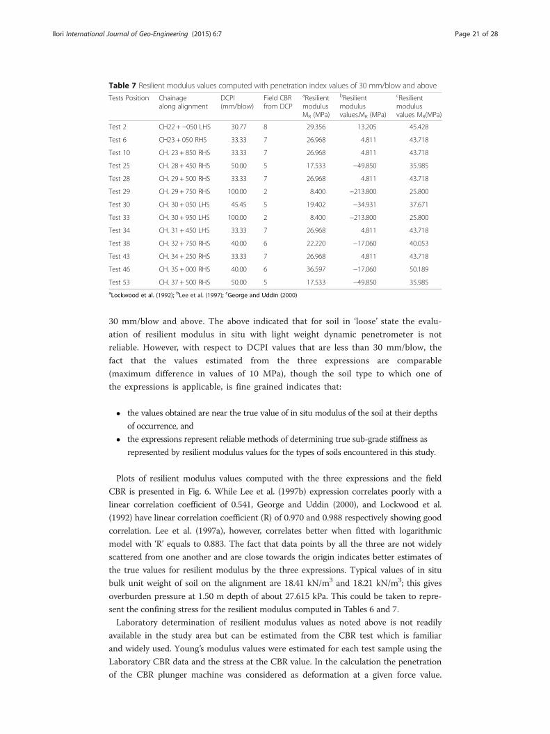
Table 7 Resilient modulus values computed with penetration index values of 30 mm/blow and above
Tests Position Chainagealong alignment
DCPI(mm/blow)
Field CBRfrom DCP
aResilientmodulusMR (MPa)
bResilientmodulusvalues.MR (MPa)
cResilientmodulusvalues MR(MPa)
Test 2 CH22 + −050 LHS 30.77 8 29.356 13.205 45.428
Test 6 CH23 + 050 RHS 33.33 7 26.968 4.811 43.718
Test 10 CH. 23 + 850 RHS 33.33 7 26.968 4.811 43.718
Test 25 CH. 28 + 450 RHS 50.00 5 17.533 −49.850 35.985
Test 28 CH. 29 + 500 RHS 33.33 7 26.968 4.811 43.718
Test 29 CH. 29 + 750 RHS 100.00 2 8.400 −213.800 25.800
Test 30 CH. 30 + 050 LHS 45.45 5 19.402 −34.931 37.671
Test 33 CH. 30 + 950 LHS 100.00 2 8.400 −213.800 25.800
Test 34 CH. 31 + 450 LHS 33.33 7 26.968 4.811 43.718
Test 38 CH. 32 + 750 RHS 40.00 6 22.220 −17.060 40.053
Test 43 CH. 34 + 250 RHS 33.33 7 26.968 4.811 43.718
Test 46 CH. 35 + 000 RHS 40.00 6 36.597 −17.060 50.189
Test 53 CH. 37 + 500 RHS 50.00 5 17.533 −49.850 35.985aLockwood et al. (1992); bLee et al. (1997); cGeorge and Uddin (2000)
Ilori International Journal of Geo-Engineering (2015) 6:7 Page 21 of 28
30 mm/blow and above. The above indicated that for soil in ‘loose’ state the evalu-
ation of resilient modulus in situ with light weight dynamic penetrometer is not
reliable. However, with respect to DCPI values that are less than 30 mm/blow, the
fact that the values estimated from the three expressions are comparable
(maximum difference in values of 10 MPa), though the soil type to which one of
the expressions is applicable, is fine grained indicates that:
� the values obtained are near the true value of in situ modulus of the soil at their depths
of occurrence, and
� the expressions represent reliable methods of determining true sub-grade stiffness as
represented by resilient modulus values for the types of soils encountered in this study.
Plots of resilient modulus values computed with the three expressions and the field
CBR is presented in Fig. 6. While Lee et al. (1997b) expression correlates poorly with a
linear correlation coefficient of 0.541, George and Uddin (2000), and Lockwood et al.
(1992) have linear correlation coefficient (R) of 0.970 and 0.988 respectively showing good
correlation. Lee et al. (1997a), however, correlates better when fitted with logarithmic
model with ‘R’ equals to 0.883. The fact that data points by all the three are not widely
scattered from one another and are close towards the origin indicates better estimates of
the true values for resilient modulus by the three expressions. Typical values of in situ
bulk unit weight of soil on the alignment are 18.41 kN/m3 and 18.21 kN/m3; this gives
overburden pressure at 1.50 m depth of about 27.615 kPa. This could be taken to repre-
sent the confining stress for the resilient modulus computed in Tables 6 and 7.
Laboratory determination of resilient modulus values as noted above is not readily
available in the study area but can be estimated from the CBR test which is familiar
and widely used. Young’s modulus values were estimated for each test sample using the
Laboratory CBR data and the stress at the CBR value. In the calculation the penetration
of the CBR plunger machine was considered as deformation at a given force value.
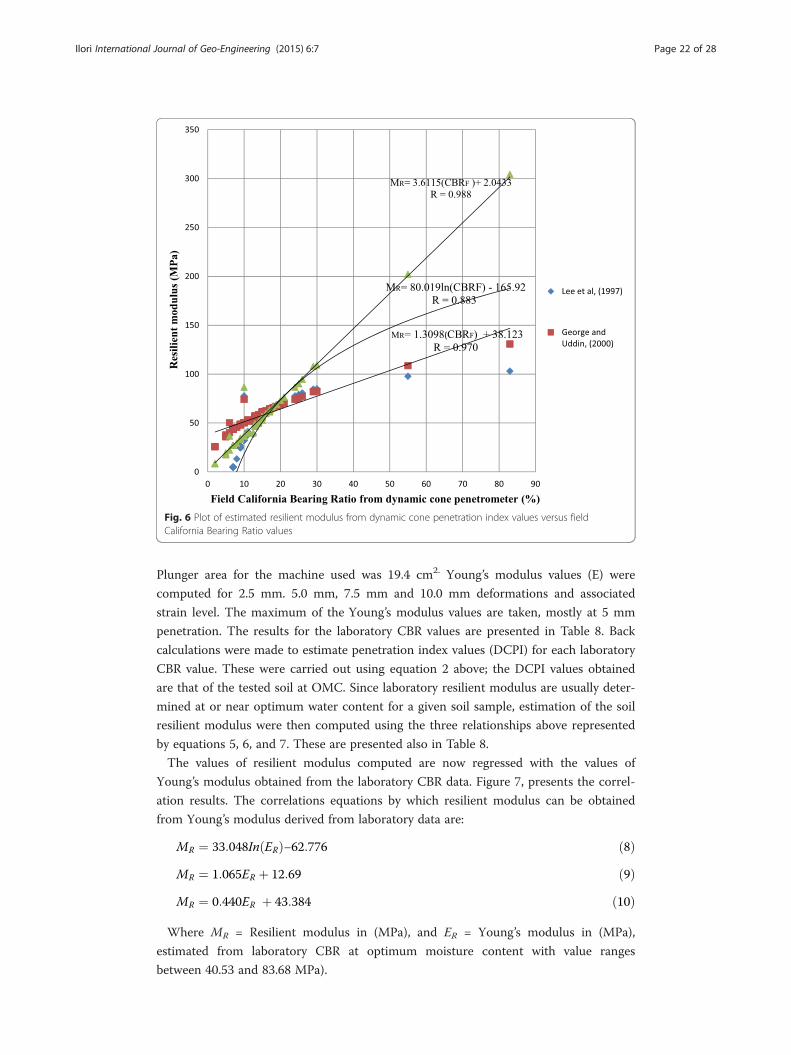
Fig. 6 Plot of estimated resilient modulus from dynamic cone penetration index values versus fieldCalifornia Bearing Ratio values
Ilori International Journal of Geo-Engineering (2015) 6:7 Page 22 of 28
Plunger area for the machine used was 19.4 cm2. Young’s modulus values (E) were
computed for 2.5 mm. 5.0 mm, 7.5 mm and 10.0 mm deformations and associated
strain level. The maximum of the Young’s modulus values are taken, mostly at 5 mm
penetration. The results for the laboratory CBR values are presented in Table 8. Back
calculations were made to estimate penetration index values (DCPI) for each laboratory
CBR value. These were carried out using equation 2 above; the DCPI values obtained
are that of the tested soil at OMC. Since laboratory resilient modulus are usually deter-
mined at or near optimum water content for a given soil sample, estimation of the soil
resilient modulus were then computed using the three relationships above represented
by equations 5, 6, and 7. These are presented also in Table 8.
The values of resilient modulus computed are now regressed with the values of
Young’s modulus obtained from the laboratory CBR data. Figure 7, presents the correl-
ation results. The correlations equations by which resilient modulus can be obtained
from Young’s modulus derived from laboratory data are:
MR ¼ 33:048In ERð Þ−62:776 ð8ÞMR ¼ 1:065ER þ 12:69 ð9ÞMR ¼ 0:440ER þ 43:384 ð10Þ
Where MR = Resilient modulus in (MPa), and ER = Young’s modulus in (MPa),
estimated from laboratory CBR at optimum moisture content with value ranges
between 40.53 and 83.68 MPa).
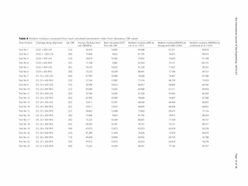
Table 8 Resilient modulus computed from back calculated penetration index from laboratory CBR values
Tests Position Chainage along alignment Lab CBR Young’s Modulus fromLab CBR(MPa)
Back calculated DCPIfrom lab CBR
Resilient modulus (MR) byLee et al. (1997)
Resilient modulus,MR(MPa) byGeorge and Uddin (2000)
Resilient modulus MR(MPa) byLockwood et al. (1992)
Test No 1 CH21 + 650 LHS 21.0 54.919 13.605 69.488 67.211 69.818
Test No 2 CH22 + −050 LHS 29.0 75.840 9.852 81.795 78.475 98.354
Test No 3 CH22 + 450 LHS 27.0 70.610 10.582 79.402 75.829 91.168
Test No 4 CH22 + 650 RHS 29.5 77.148 9.685 82.343 79.121 100.155
Test No 5 CH22 + 850 LHS 28.5 74.533 10.025 81.228 77.822 96.555
Test No 6 CH23 + 050 RHS 28.0 73.225 10.204 80.641 77.164 94.757
Test No 7 CH. 23 + 250 LHS 26.0 67.995 10.989 78.068 74.467 87.588
Test No 8 CH. 23 + 450 RHS 22.0 57.534 12.987 71.516 68.729 73.353
Test No 9 CH. 23 + 650 LHS 19.5 50.996 14.652 66.057 64.863 64.536
Test No 10 CH. 23 + 850 RHS 21.0 83.686 13.605 69.488 67.211 69.818
Test No 11 CH. 24 + 050 LHS 20.0 52.304 14.285 67.258 65.656 66.294
Test No 12 CH. 24 + 250 RHS 26.0 67.995 10.989 78.068 74.467 87.588
Test No 13 CH. 24 + 450 LHS 20.5 53.611 13.937 68.400 66.438 68.055
Test No 14 CH. 24 + 650 RHS 20.5 53.611 13.937 68.400 66.438 68.055
Test No 15 CH. 25 + 050 RHS 22.5 58.842 12.698 72.463 69.475 75.124
Test No 16 CH. 25 + 450 RHS 29.0 75.840 9.852 81.795 78.475 98.354
Test No 17 CH. 25 + 650 RHS 28.0 73.225 10.204 80.641 77.164 94.757
Test No 18 CH. 25 + 850 RHS 26.5 69.302 10.781 78.747 75.151 89.377
Test No 19 CH. 26 + 250 RHS 18.0 47.073 15.873 62.053 62.418 59.278
Test No 20 CH. 26 + 650 RHS 25.0 65.380 11.428 76.626 73.078 84.016
Test No 21 CH. 26 + 850 RHS 17.0 44.458 16.806 58.992 60.729 55.788
Test No 22 CH. 27 + 250 RHS 18.0 47.073 15.873 62.053 62.418 59.278
Test No 23 CH. 27 + 650 RHS 28.0 73.225 10.204 80.641 77.164 94.757
IloriInternationalJournalofGeo-Engineering
(2015) 6:7 Page
23of
28
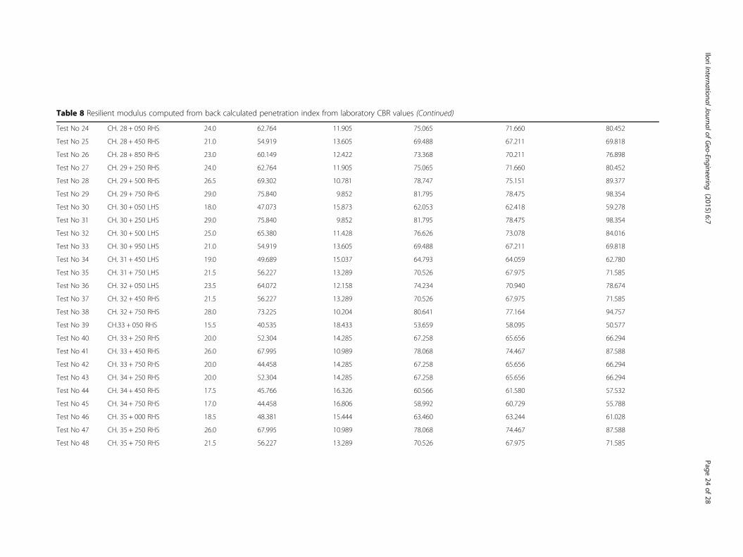
Table 8 Resilient modulus computed from back calculated penetration index from laboratory CBR values (Continued)
Test No 24 CH. 28 + 050 RHS 24.0 62.764 11.905 75.065 71.660 80.452
Test No 25 CH. 28 + 450 RHS 21.0 54.919 13.605 69.488 67.211 69.818
Test No 26 CH. 28 + 850 RHS 23.0 60.149 12.422 73.368 70.211 76.898
Test No 27 CH. 29 + 250 RHS 24.0 62.764 11.905 75.065 71.660 80.452
Test No 28 CH. 29 + 500 RHS 26.5 69.302 10.781 78.747 75.151 89.377
Test No 29 CH. 29 + 750 RHS 29.0 75.840 9.852 81.795 78.475 98.354
Test No 30 CH. 30 + 050 LHS 18.0 47.073 15.873 62.053 62.418 59.278
Test No 31 CH. 30 + 250 LHS 29.0 75.840 9.852 81.795 78.475 98.354
Test No 32 CH. 30 + 500 LHS 25.0 65.380 11.428 76.626 73.078 84.016
Test No 33 CH. 30 + 950 LHS 21.0 54.919 13.605 69.488 67.211 69.818
Test No 34 CH. 31 + 450 LHS 19.0 49.689 15.037 64.793 64.059 62.780
Test No 35 CH. 31 + 750 LHS 21.5 56.227 13.289 70.526 67.975 71.585
Test No 36 CH. 32 + 050 LHS 23.5 64.072 12.158 74.234 70.940 78.674
Test No 37 CH. 32 + 450 RHS 21.5 56.227 13.289 70.526 67.975 71.585
Test No 38 CH. 32 + 750 RHS 28.0 73.225 10.204 80.641 77.164 94.757
Test No 39 CH.33 + 050 RHS 15.5 40.535 18.433 53.659 58.095 50.577
Test No 40 CH. 33 + 250 RHS 20.0 52.304 14.285 67.258 65.656 66.294
Test No 41 CH. 33 + 450 RHS 26.0 67.995 10.989 78.068 74.467 87.588
Test No 42 CH. 33 + 750 RHS 20.0 44.458 14.285 67.258 65.656 66.294
Test No 43 CH. 34 + 250 RHS 20.0 52.304 14.285 67.258 65.656 66.294
Test No 44 CH. 34 + 450 RHS 17.5 45.766 16.326 60.566 61.580 57.532
Test No 45 CH. 34 + 750 RHS 17.0 44.458 16.806 58.992 60.729 55.788
Test No 46 CH. 35 + 000 RHS 18.5 48.381 15.444 63.460 63.244 61.028
Test No 47 CH. 35 + 250 RHS 26.0 67.995 10.989 78.068 74.467 87.588
Test No 48 CH. 35 + 750 RHS 21.5 56.227 13.289 70.526 67.975 71.585
IloriInternationalJournalofGeo-Engineering
(2015) 6:7 Page
24of
28
Table 8 Resilient modulus computed from back calculated penetration index from laboratory CBR values (Continued)
Test No 49 CH. 36 + 000 RHS 23.5 61.457 12.158 74.234 70.940 78.674
Test No 50 CH. 36 + 550 RHS 20.0 52.304 14.285 67.258 65.656 66.294
Test No 51 CH. 37 + 120 LHS 20.0 52.304 14.285 67.258 65.656 66.294
Test No 52 CH. 37 + 250 RHS 20.0 52.304 14.285 67.258 65.656 66.294
Test No 53 CH. 37 + 500 RHS 22.5 45.766 12.698 72.463 69.475 75.124
Test No 54 CH. 37 + 750 LHS 25.0 44.458 11.428 76.626 73.078 84.016
Test No 55 CH. 38 + 400 RHS 18.5 65.380 15.444 63.460 63.244 61.028
IloriInternationalJournalofGeo-Engineering
(2015) 6:7 Page
25of
28
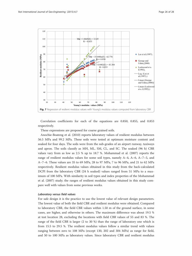
Fig. 7 Regression of resilient modulus values with Young’s modulus values computed from laboratory CBR
Ilori International Journal of Geo-Engineering (2015) 6:7 Page 26 of 28
Correlation coefficients for each of the equations are 0.850, 0.855, and 0.853
respectively.
These expressions are proposed for coarse grained soils.
Anochie-Boateng et al. (2010) reports laboratory values of resilient modulus between
56.5 MPa and 99.2 MPa. These soils were tested at optimum moisture content and
soaked for four days. The soils were from the sub-grades of an airport runway, taxiways
and apron. The soils classify as MH, ML, SM, CL, and SC. The soaked (96 h) CBR
values vary from as low as 2.5 % up to 18.7 %. Mohammad et al. (2007) reports the
range of resilient modulus values for some soil types, namely A–4, A–6, A–7–5, and
A–7–6. These values are 35 to 69 MPa, 28 to 97 MPa, 7 to 96 MPa, and 21 to 62 MPa
respectively. Resilient modulus values obtained in this study from the back-calculated
DCPI from the laboratory CBR (24 h soaked) values ranged from 51 MPa to a max-
imum of 100 MPa. With similarity in soil types and index properties of the Mohammad
et al. (2007) study; the ranges of resilient modulus values obtained in this study com-
pare well with values from some previous works.
Laboratory versus field values
For safe design it is the practice to use the lowest value of relevant design parameters.
The lowest value of both the field CBR and resilient modulus were obtained. Compared
to laboratory CBR, the field CBR values within 1.50 m of the ground surface, in some
cases, are higher, and otherwise in others. The maximum difference was about 19.5 %
at test location 28, excluding the locations with field CBR values of 55 and 83 %. The
range of the field CBR is larger (2 to 30 %) than the range of laboratory one which is
from 15.5 to 29.5 %. The resilient modulus values follow a similar trend with values
ranging between zero to 108 MPa (except 130, 202 and 304 MPa) as range for field,
and 50 to 100 MPa as laboratory values. Since laboratory CBR and resilient modulus
Ilori International Journal of Geo-Engineering (2015) 6:7 Page 27 of 28
are to serve as control for field earthworks operations this implies that the desired field
CBR values can easily be achieved and, in some cases, surpass desired values. With
respect to resilient modulus, the field values were the least available in situ; for those
locations with values less than 50 MPa (the minimum laboratory value) the field resili-
ent modulus values have to be brought up to this value at those locations. The above
strongly suggests that field resilient modulus values obtained using the LRS 10 pene-
trometer adequately estimate sub-grade stiffness required for design purposes for a
given pavement.
ConclusionsThe highway alignment is characterized by sandy and silty soil types within 0 to 6.0 m
depth investigated. These soil types are Clayey Sand, SC (A-2-6), Silty Sand SM(A-2-7),
and a combination of the two, SC- SM (A-6). There is occurrence of MH, OH and ML
(A-7-5) soil types within stretches of the alignment as shown by four test points. These
soil types are consistent with the geology of the area. Based on soil consistency as indi-
cated by relative density, a light weight Penetrometer was able to characterize the align-
ment in to three zones in both depth and areal extent, adequate for the proposed
pavement. AASHTO classification rate as “good”, a significant stretch of the sub-grade
alignment based on both the in situ CBR and the lowest laboratory CBR values.
The sub-grade stiffness as indicated by both in situ tests with LRS 10 and estimated
resilient modulus values for a reasonable portion of the highway alignment is adequate;
however, improvement of the relatively ‘loose’ by deep compaction sections will need
to be required.
Correlation was established for the type of soil encountered in this study between
CBR and relative density, and between penetration index and relative density. Similarly,
a relationship was established between resilient modulus and Young’s modulus. The
latter can easily be evaluated from laboratory CBR tests.
Competing interestsThe author declares they have no competing interests.
AcknowledgementsI wish to acknowledge and appreciate Robin Williams, Administrative. Assistant at Grant African Methodist EpiscopalChurch in Toronto, Ontario, Canada. who helped with the proof reading of the article; and Messers Moshood A. Sakaand Lanre Aroyewun who helped in the laboratory analyses.
Received: 11 October 2014 Accepted: 20 July 2015
References
Anochie-Boateng, J., Tutumluer, E., Apeagyei, A., and Ochieng, G. (2010). Resilient behavior characterization ofgeomaterials for pavement design. ISAP Nagoya 9 (2010), 11th International Conference on Asphalt Pavements,Nagoya, Japan, August 1–6, 2010: p. 10. http://hdl.handle.net/10204/4412(16/4/2014)
ASTM D-1586 (2011). Standard Test Method for Standard Penetration Test (SPT) and Split-Barrel Sampling of Soils.Begemann, H.K. (1965). “The friction jacket cone as an aide in determining the soil profile”, Proceedings, 6th
International Conference on Soil Mechanics and Foundation Engineering, Vol. 1, Montreal, pp. 17–20.Campanella, RG., Gillespie, D., & Robertson, P.K. (1982). Pore pressures during cone penetration testing. In Proceedings of
the 2nd European Symposium on Penetration Testing, ESPOT II (pp. 507–512). Amsterdam: A.A.Balkema.Chen, D.H., Lin, DF., Pen-Hwang Liau P.H., Bilyeu, J. (2005). A correlation between Dynamic Cone Penetrometer values
and pavement layer moduli, Geotechnical Testing Journal, 38 (1).Das, B.M. (1983). Advanced soil mechanics (p. 34). New York: McGraw- Hill Book Company. 442.De Beer, M., and CJ van der Merwe. (1991). Use of the Dynamic Cone Penetrometer (DCP) in the design of road structures,
Minnesota Department of Transportation, St. Paul.DIN 4094, Part 2 (1980). Dynamic and Static Penetrometer.
Ilori International Journal of Geo-Engineering (2015) 6:7 Page 28 of 28
Done, S., and Samuel, P. (2006). Department for International Development (DFID). Measuring road pavement strengthand designing low volume sealed roads using the dynamic cone penetrometer. Unpublished Project Report,UPR/IE/76/06. Project Record No. R7783. www.transport-links.org/ukdcp/docs/Manual/manual.html -(18/4/2014)
FHWA NHI-05-037 (2006). Geotechnical aspects of pavement. U.S. Department of Transportation Federal HighwayAdministration. Pp4-17.
George, K.P., & Uddin, W. (2000). Subgrade characterization for highway pavement design, final report. Jackson, MS:Mississippi Department of Transportation.
Irwin, L. (2009). Resilient modulus test. federal highway administration Technical Advisory Committee (TAC) on resilientmodulus test procedures for unbound materials. Pooled Fund Project TPF-5(177). http://www.resilientmodulus.com/index.php?q=system/files/Lynne_Irwin.pdf
Jaksa, M.B., Scott, B.T., Mentha, N.L., Symons, A.T., Pointon, S.M., Wrightson, P.T., and Syamsuddin, E. (2012). Quantifying thezone of influence of the impact roller. ISSMGE - TC 211 International Symposium on Ground Improvement IS-GI Brussels
Kloubert, H-J. (2009). Single drum roller with polygonal drum for deep compaction and thick lift compactionapplications. BOMAG GmbH, Germany. http://www.bomag.com/de/media/file/Polygon-March-2009-en.pdf
Lee, W., Bohra, N.C., Altschaeffl, A.G., & White, T.D. (1997a). Resilient modulus of cohesive soils. Journal of Geotechnicaland Geoenvironmental Engineering, 123(2), 131–136.
Lee, W., Bohra, N.C., & Altschaeffl, A.G. (1997b). Resilient characteristics of dune sand. Journal of TransportationEngineering, ASCE, 121(6), 502–506.
Lockwood, D., de Franca, V.M.P., Ringwood, B., & de Beer, M. (1992). Analysis and classification of DCP survey data.Technology and information management programme. Pretoria, South Africa: CSIR Transportek.
Mohammad, L.N., Gaspard, K., Herath, A., & Nazzal, M.D. (2007). Comparative evaluation of subgrade resilient modulusfrom non-destructive, In-situ, and laboratory methods (p. 30). LA, US: Louisiana Transportation Research Center.
Nigerian Geological Survey Agency, (2006). Geological and Mineral Map of Akwa-Ibom State, Nigeria.Olsen, R.S., and Farr, J.V. (1986). Site characterization using the cone penetration Test. Proceedings, In-Situ’86. ASCE
specialty conference,Blacksburg. Virginia Pavementinteractive.org,2007.ResilientModulus.www.pavementinteractive.org/article/resilientmodulus.
Peck, R.P., Hanson, E., & Thornburn, T.H. (1974). Foundation engineering (2nd ed., p. 28,337). New York: John Wiley and Sons.Pen, C.K. (1990). An assessment of the available methods of analysis for estimating the elastic moduli of road
pavements, in Proc. 3rd Int. Conference on Bearing Capacity of Roads and Airfields, Trondheim.Robertson, P.K. (1990). Soil classification using the cone penetration test. Canadian Geotechnical Journal, 27, 151–158.Sowers, G.F., and Hedges, C.S. (1966). “Dynamic cone for shallow In-Situ penetration testing,” Vane Shear and cone
penetration resistance testing of In-Situ soils, ASTM STP 399, American Society of Testing Materials. pp. 29.Transport and Road Research Laboratory. (1990). A user’s manual for a program to analyse dynamic cone penetrometer
data (Overseas Road Note 8). Crowthorne: Transport Research Laboratory.Vandre, B., Budge, A., and Nussbaum, S. (1998).“DCP- A Useful Tool for Characterizing Engineering Properties of Soils at
Shallow Depths. Proceedings of 34th Symposium on Engineering Geology and Geotechnical Engineering, UtahState University, Logan, UT.
Submit your manuscript to a journal and benefi t from:
7 Convenient online submission
7 Rigorous peer review
7 Immediate publication on acceptance
7 Open access: articles freely available online
7 High visibility within the fi eld
7 Retaining the copyright to your article
Submit your next manuscript at 7 springeropen.com