geostatistical evaluation of magnetic indicators of forest soil contamination with heavy metals

Stud. Geophys. Geod., 53 (2009), 133−149 133 © 2009 Inst. Geophys. AS CR, Prague

GEOSTATISTICAL EVALUATION OF MAGNETIC INDICATORS OF FOREST SOIL CONTAMINATION WITH HEAVY METALS

JAROSŁAW ZAWADZKI1, TADEUS MAGIERA2 AND PIOTR FABIJAŃCZYK1

1 Warsaw University of Technology, Environmental Engineering Systems Institute, Nowowiejska 20, 00-661 Warszawa, Poland ([email protected], [email protected])

2 Institute of Environmental Engineering, Polish Academy of Science, M. Curie-Skłodowskiej 34, 41-819 Zabrze, Poland ([email protected])

Received: February 21, 2008; Revised: May 30, 2008; Accepted: June 6, 2008

ABSTRACT

The goal of the study was the geostatistical evaluation of quantitative magnetic measures, which can be used for effective delineation of the extent of the area polluted with heavy metals. Several parameters of magnetic susceptibility, measured in the soil profile, were proposed as magnetic indicators of soil pollution and analyzed in detail. The following parameters were calculated: maximum magnetic susceptibility, magnetic susceptibility at the depth of 3 cm and 5 cm, and the area under the curve of magnetic susceptibility. Measurements were performed at two forested study areas, located in Upper Silesian Industrial Area (Poland). Analyses were performed using geostatistical methods, and the results were verified using dense chemical measurements.

The results showed that the area under curve of magnetic susceptibility was the most effective magnetic indicator of soil contamination with heavy metals. It was possible to detect the entire polluted area, and only about 16% of the study area was assumed to be contaminated while being unpolluted. The results obtained with maximum magnetic susceptibility and magnetic susceptibility at the depth of 3 cm and 5 cm were less effective in comparison with the area under curve of magnetic susceptibility.

Ke y wo rd s : geostatistics, heavy metals, magnetic susceptibility, quantitative

indicator, soil profile, soil pollution

1. INTRODUCTION

Field magnetometry is a fast and cost-effective method used to detect and assess the level and extent of soil contamination caused by anthropogenic or industrial pollution (Boyko et al., 2004; Chianese et al., 2005; Desenfant et al., 2004; Hanesh and Scholger, 2002; Kapička et al., 1999; Petrovský et al., 2000; Strzyszcz, 1993; Strzyszcz et al., 1996; Hanesch, 2002). Industrial dusts that are deposited on the soil surface contain significant

J. Zawadzki et al.

134 Stud. Geophys. Geod., 53 (2009)

amounts of ferromagnetic iron oxides and heavy metals. Consequently, the soil magnetic susceptibility is correlated positively in a significant way with the concentration of heavy metals in soil (Georgeaud et al., 1997; Oldfield et al., 1985; Schibler et al., 2002; Spitieri et al., 2005; Strzyszcz and Magiera, 2001; Thomson and Oldfield, 1986; Wang and Qin, 2005). However, it is difficult to explain mechanisms of these correlations in detail because they depend on a variety of complex and coactive physicochemical, pedological or environmental factors.

Numerous studies of soil pollution with field magnetometry, were focused on analyzes of classic correlations or alternatively on analyzes of simple linear regression between magnetometric and chemical measurements. The number of geostatistical studies of spatial correlations among those measurements is still limited (Magiera and Zawadzki, 2006; Zawadzki and Fabijańczyk, 2007). The knowledge of spatial correlations between magnetometric and chemical measurements can be useful when comparing the extents of polluted area delineated using both types of measurements. Frequently, geostatistical methods also help to improve the precision of analyses, and to interpret appropriately the results afterwards. In consequence, it is possible to increase the effectiveness of field magnetometry.

Most of the studies of soil pollution with field magnetometry were focused rather on measurements of surface soil magnetic susceptibility, typically performed with a MS2D Bartington sensor (Dearing, 1994). Measurements of magnetic susceptibility in soil profile (vertical measurements) were seldom used. This may be caused by the fact that this kind of measurement is more complicated and time-consuming in comparison with the surface one. On the other hand, vertical measurement is more precise than the surface one and gives more information about the soil magnetic susceptibility at sampled location. They are also significantly correlated with the concentration of heavy metals in soil (Spiteri et al., 2005). Moreover, vertical measurements are also more resistant to possible measuring errors caused by varying thickness and the degree of development of soil layers, especially the uppermost ones. For that reasons and due to limited penetration range, values measured with a MS2D sensor can be often biased with some errors, and observed correlations between magnetic susceptibility and the concentration of heavy metals in soil may be insignificant (Zawadzki et al., 2007). Frequently, the peak value of magnetic susceptibility in the soil profile and the highest concentration of heavy metals are observed at the same depth. In addition, the distribution of magnetic susceptibility in the soil profile reflects the thickness of soil subhorizons, in particular the organic and humic ones, where most of the heavy metals are accumulated. Up to now, vertical measurements were mostly used to distinguish the differences between the magnetic enhancements caused by anthropogenic pollution or lithogenic origin (Magiera et al., 2006) or to investigate in which soil horizons the most of heavy metals are accumulated (Magiera et al., 2006; Fialová et al. 2006). The quantitative relation between the concentration of heavy metals and magnetic susceptibility in the soil profile was not analyzed in detail. However, some authors (Spiteri et al., 2005) indicated that it might be advantageous to use the area under the curve of magnetic susceptibility as an indicator of soil pollution with heavy metals.

The goal of this paper was to find reliable magnetic measures inferred from measurements of magnetic susceptibility in the soil profile, which can be effectively used to assess the extent of area polluted with heavy metals. To do so, several magnetic

Geostatistical Evaluation of Magnetic Indicators of Soil Contamination

Stud. Geophys. Geod., 53 (2009) 135

indicators, as maximum magnetic susceptibility, magnetic susceptibility at specified depths, and the area under the curve of magnetic susceptibility, were proposed and discussed. Those magnetic indicators were used to model the extent of potentially polluted area, which was subsequently verified using chemical measurements and advanced geostatistical method, namely, indicator kriging. Such procedure made it possible to assess the most effective threshold values of investigated magnetic indicators, which can be used during next measurements campaigns. The analyses were performed separately at two study areas located within the Upper Silesian Industrial Area (USIA) in Poland.

2. STUDY AREAS

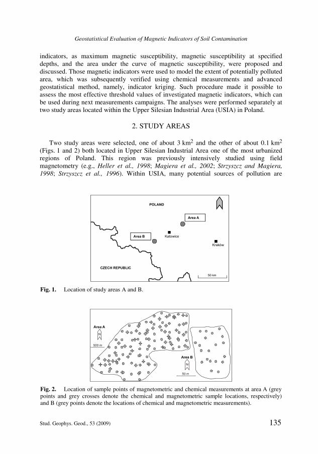
Two study areas were selected, one of about 3 km2 and the other of about 0.1 km2 (Figs. 1 and 2) both located in Upper Silesian Industrial Area one of the most urbanized regions of Poland. This region was previously intensively studied using field magnetometry (e.g., Heller et al., 1998; Magiera et al., 2002; Strzyszcz and Magiera, 1998; Strzyszcz et al., 1996). Within USIA, many potential sources of pollution are

Fig. 1. Location of study areas A and B.

Fig. 2. Location of sample points of magnetometric and chemical measurements at area A (grey points and grey crosses denote the chemical and magnetometric sample locations, respectively) and B (grey points denote the locations of chemical and magnetometric measurements).

J. Zawadzki et al.


present due to an intensive industrial and mining activity. In soils of this region, high concentrations of heavy metals are frequently observed, repeatedly exceeding maximum allowable levels (Magiera et al., 2007). In order to reduce the significant anthropogenic influx, the study areas were located in pine forests with podzolic soils far from the Katowice agglomeration. The analysis made for different soil types in Central Europe showed that there are seven types of vertical susceptibility distribution (Magiera et al., 2006). For both study areas, the profiles of magnetic susceptibility showed the typical characteristics of sandy ferric podzols with strong anthropogenic influence (the type of profile denoted by Magiera et al., 2006 as “A1”).

The larger area, denoted by the letter A, was located about 30 km to the east of Katowice agglomeration in an old pine forest. A total of 49 measurements of volume magnetic susceptibility in soil profile, and 67 chemical measurements were performed, following a regular sampling grid (Fig. 2). The chemical and magnetometric measurements were carried out at different sample locations, and the average spacing between sample locations of magnetometric measurements equaled 250 to 350 m, and 200 to 250 m for chemical ones. The dense chemical measurements served as a reference set for magnetometric ones.

The smaller area, denoted by the letter B, was located near Szczejkowice town in the southern part of USIA also in a pine forest. At this area, 19 sample points were located, and at each one, chemical and magnetometric measurements were performed.

3. MATERIALS AND METHODS

3 . 1 . M a g n e t o m e t r i c M e a s u r e m e n t s

Field measurements of volume magnetic susceptibility in soil profile were performed by using a SM400 device (Petrovský et. al., 2004; Spitieri et. al., 2005). The measurements were performed down to the depth of 30 cm, which is the same as a length of soil cores collected in the field. The probe of SM400 was inserted into the drilled hole for measuring magnetic susceptibility. The sensor located into the plastic tube moved up and down the soil profile. After that, data were transferred to the computer (laptop) and then the plot of soil magnetic susceptibility against the depth was drown.

In order to find the most effective indicators of soil pollution, the following parameters of magnetic susceptibility in soil profile were determined (compare with Fig. 3):

(i) maximum magnetic susceptibility in soil profile (abbreviated hereafter as κmax) (ii) the value of magnetic susceptibility at depths of 3 and 5 cm (abbreviated

hereafter as κ3cm and κ5cm, respectively) (iii) the area under the curve of magnetic susceptibility in soil profile between the soil

surface and the depth where the curve stabilizes (abbreviated hereafter as Aκ) - marked in the Fig. 3 in gray.

Accordingly to the previous studies (Magiera et al., 2006) there is a significant difference between the magnetic enhancement of lithogenic and anthropogenic origin. In case of anthropogenic pollution, magnetic susceptibility increases rapidly along the depth (see Fig. 3), next reaches maximum value at the depth of about 3 to 5 cm, and after that



decreases rapidly with increasing depth. At some depth, the magnetic susceptibility begins to be almost constant or changes insignificantly. The initial depth where it was observed was assumed as the depth where the magnetic susceptibility stabilizes. Since the Aκ reflects a total magnetic enhancement caused by anthropogenic pollution, it is strongly correlated with the total concentration of heavy metals in soil (Spiteri et al., 2005). All plots of magnetic susceptibility, measured at both study areas, were found to be characteristic for anthropogenic pollution.

It was possible to calculate precisely the Aκ by using the raw output from a SM400 meter and the trapezoidal integration (Karris, 2007). The raw data involve a large number of readings done by a SM400 meter with very high density. Typical lag between depths, at which magnetic susceptibility was measured, ranged from 0.1 to 0.3 mm.

3 . 2 . C h e m i c a l M e a s u r e m e n t s

The concentration of heavy metals in soil was determined using soil samples collected in the field, and was expressed in mg/kg. At study Area A, soil samples with weight of about 0.5 kg were taken from a depth of 0 to 20 cm using a soil corer of 8 cm diameter. Soil samples were dried at room temperature and sieved through a 1mm sieve. After that, samples were diminished by means of quartage, and subsequently water sediments were sieved through the 0.2 mm sieve. Afterwards, samples were digested using 1:5 HCl at the temperature of 90°C during 1 hour. As the result, the analytical samples with weight of 100 g were obtained. For each soil profile, one analytical sample was obtained. Next, each such sample was used to measure the concentration of Cd, Cu, Ni, Pb and Zn by using emission spectrometer with Inductively Coupled Plasma (ICP).

In case of the Area B, 30 cm long and 3.5 cm diameter soil samples were collected using a Humax soil corer. The sub-samples were cut from the part of cores where the

Fig. 3. Scheme of indicators inferred from plots of magnetic susceptibility in soil profile: maximum value of susceptibility (κmax), the value at specified depth (κ3cm and κ5cm) and the area under the curve from surface to the depth where magnetic susceptibility stabilizes (Aκ).

J. Zawadzki et al.


highest values of magnetic susceptibility were observed, which usually ranged from 2 cm to 8 cm. Soil samples were dried at room temperature, and then sieved through a 1 mm sieve, and afterwards digested using 2M HNO3. Finally, the concentration of Cd, Cu, Ni, Pb and Zn was measured using Atomic Absorption Spectrometer (AAS).

3 . 3 . G e o s t a t i s t i c a l A p p r o a c h

The spatial distributions of the concentration of particular heavy metals in soil were modeled using both ordinary and indicator kriging. Ordinary kriging is the most effective linear estimator as it assumes that the average value of the estimation error equals zero, and the variance of estimation error is simultaneously minimized (Goovaerts, 1997). The kriging estimation at the unsampled location u0(x0) is made using values from n neighboring measurement points ui(x) weighted by weights ai(x). Kriging weights λi(x) are determined using a semivariance function and are chosen for each sample point within search radius:

( ) ( ) ( )0 01

n

i ii

u uλ=

=∑x x x . (1)

Search radius usually depends on the distance of correlation, which is expressed by the range of a variogram model.

Application of indicator kriging demands the data to be transformed using some specified threshold values (Goovaerts, 1997; Isaaks and Srivastava, 1989). In this study, indicator kriging was used to model the extent of polluted area. Consequently, the threshold values were equal to the maximum allowable concentrations of particular heavy metals and were picked up according to the Polish norms for the proper class of terrain usage and the depth, at which samples where collected. They equaled 4, 150, 100, 100 and 300 mg/kg for Cd, Cu, Ni, Pb and Zn, respectively. Each i-th (from n samples) measured value Z(xi) was compared with the threshold value C. If it was greater or equal, it was assigned with one, in other case it was assigned with zero:

( ) ( )( )

0 if

1 ifi

ii

Z x CI

Z x C

⎧ <⎪= ⎨ ≥⎪⎩x . (2)

After the transformation of data set, kriging method was applied using binary data. At unsampled locations, the values of probability P(x) were calculated as a sum of Ii(x) multiplied by kriging weights λi:

( ) ( )1

n

i ii

P Iλ=

=∑x x . (3)

In the result, the map that presents the probability of exceeding the threshold value is obtained. This technique is more precise than ordinary kriging, especially when analyzed datasets have non-Gaussian, skewed or multimodal distribution, which is common for soil pollution data (Goovaerts, 1997).



At the Area B, spatial distributions were obtained using Inverse Distance Weighting method (Isaaks and Srivastava, 1989), because of the small dataset of chemical and magnetometric measurements. The number of samples was not enough to calculate a reliable variogram and then apply indicator kriging.

3 . 4 . D e t e r m i n a t i o n o f M a g n e t i c I n d i c a t o r s a n d T h e i r T h r e s h o l d s

All analyses of spatial distributions were carried out using grid maps, namely the entire study area was divided into 2880 square blocks (50 × 50 m) and each i-th block was assigned with the estimated value. The most effective values of magnetic indicators were determined by a comparison of such grided spatial distributions of particular magnetic indicators, block by block, with those obtained using the dense chemical measurements. The geostatistical analysis was carried out using ArcGis 9 with Geostatistical Analyst extension (ESRI, 2004).

The spatial distributions for Cd, Cu, Ni, Pb and Zn were modeled by means of indicator kriging taking the above-cited maximum allowable concentrations of heavy metal in the soil (that is 4, 150, 100, 100 and 300 mg/kg for Cd, Cu, Ni, Pb and Zn, respectively) as threshold values C (see Eq.(2)). The probability map of exceeding the maximum allowable concentration was determined for each investigated heavy metal.

Subsequently, for each heavy metal the extent of polluted area was estimated using the above-described grided probability maps. The block was assumed to be polluted with particular heavy metal (Cd, Cu, Ni, Pb or Zn) if the probability of exceeding maximum allowable concentration Pmax for this metal was greater than 50%. Otherwise, the block was assumed to be not polluted by this heavy metal. In the result, for each heavy metal one binary map (with values 0 or 1) was obtained:

1 if 50%

0 if 50%max

max

PA

P

≥⎧= ⎨ <⎩

. (4)

Afterward, those five grided maps were combined to a single spatial distribution of the overall extent of polluted area, denoted hereafter by Aoverall. This combination was performed in this way that block was assumed to be polluted, and assigned with 1, if it was polluted by at least one heavy metal. Otherwise, the block was assumed to be clean, and assigned with 0 (i.e. if it was not polluted by any of the investigated heavy metals).

Next, the spatial distributions of κmax, κ3cm, κ5cm and Aκ were modeled using ordinary kriging. Subsequently, each of those four spatial distributions was transformed to binary maps according to Eq.(5) and using threshold values Ts listed in the Table 1. As it can be seen in this table, the threshold values Ts were chosen with rather dense interval of

5.0 × 10−3 SI for κmax, κ3cm, κ5cm or 5.0 mm × 10−3 SI for Aκ (for the sake of clarity, the subscript s, which enumerates the threshold values will be omitted when unnecessary). A block was assigned with one if its value estimated with ordinary kriging MOK greater than the considered threshold value Ts, otherwise the block was assigned with zero:

J. Zawadzki et al.


1 if

0 ifOK s

sOK s

M TM

M T

≥⎧= ⎨ <⎩

. (5)

In the result, the 25 maps were obtained, eight maps for κmax, six for κ3cm, five for κ5cm and six for Aκ. Afterward, each one of these 25 maps was compared with a map of

an overall extent of the polluted Area Aoverall. The comparison was also done block by block:

overalls sV A M= − . (6)

The Aoverall and Ms grided maps had only binary values, so after subtraction the Vs can be equal only to −1, 0 or 1. These values of Vs indicate that the extent of polluted area was overestimated, exactly estimated, or underestimated, respectively. After the comparison, it was possible to calculate the number of over- and underestimated blocks, and knowing its size, also the over- and underestimated area. For each magnetic indicator, the investigated threshold value was assumed being the most effective, when the following assumptions were fulfilled:

(i) there was no area with underestimated level of pollution, and the entire polluted area was detected using magnetic indicator

(ii) the extent of the area with overestimated level of pollution (e.g., where clean area was treated as contaminated) was minimal

All modeled spatial distributions of magnetic indicators were validated using cross-validation method. Each of the data points was individually removed from the domain, and after that, its value was modeled and subsequently compared with the measured one. Next, the scatter plots of estimated values versus the measured ones were calculated. Using these scatter plots the correlation coefficient and several estimation errors were calculated. For each of the modeled spatial distributions the particular errors were minimized, while the correlation coefficient was maximized. Furthermore, modeled spatial distributions were validated using chemical measurements, which was discussed in the further part of the article.

Table 1. Threshold values Ts used for magnetic indicators κmax, κ3cm, κ5cm and Aκ.

Magnetic Indicator Threshold Values Ts Number of Thresholds

κmax [10−3 SI] 105, 110, ..., 140 8 (s = 1, ..., 8)

κ3cm [10−3 SI] 65, 70, ..., 90 6 (s = 1, ..., 6)

κ5cm [10−3 SI] 85, 90, ..., 105 5 (s = 1, ..., 5)

Aκ [mm × 10−3 SI] 70, 75, ..., 95 6 (s = 1, ..., 6)



4. RESULTS AND DISCUSSION

4 . 1 . O v e r a l l E x t e n t o f P o l l u t e d A r e a

At the beginning of the analysis, the descriptive statistics were calculated for measured concentrations of Cd, Cu, Ni, Pb and Zn in soil, as well as for magnetic indicators κmax, κ3cm, κ5cm and Aκ (Table 2). These statistics were calculated separately for study areas A and B. At the Area A, the concentrations of Cd, Pb and Zn exceeded the maximum allowable concentrations at five, sixteen, and three sample locations, respectively. The concentrations of Cu and Ni were considerably lower than critical values and reached only 10% and 3% of maximum allowable concentrations, respectively.

At the Area A, modeled spatial distributions showed that maximum probability of exceeding the critical level of Pb was very high, reaching 0.89 in the southwestern part of the study area (Fig. 4). The probability that Cd concentration will exceed critical level was significantly lower, up to 0.37 in the southern and southwestern part of the study area. In case of Zn, this probability was even smaller, up to 0.20 in the southern part. Accordingly, the concentration values of Pb in soil had the largest effect on the delineation of the combined polluted area, with Cd and Zn concentrations contributing to a lesser amount.

Table 2. Descriptive statistics of heavy metals concentration in soil and magnetic indicators for both study areas A and B.

Min. Max. Avg. Median Std. Dev.

Are

a A

Cd

[mg/kg]

0.3 8.0 1.6 1.1 1.5 Cu 1.0 15.0 5.6 5.0 3.5 Ni 1.0 9.0 3.1 1.5 2.6 Pb 15.0 160.0 67.4 57.8 37.1 Zn 9.0 352.0 107.4 76.0 82.4

κmax

[10−3 SI]

64.1 229.5 128.1 131.2 36.2 κ3cm 0.0 160.3 67.2 60.5 39.7 κ5cm 13.6 217.5 92.6 92.8 43.8

Aκ [mm × 10−3 SI] 22.0 157.9 78.8 77.1 28.1

Are

a B

Cd

[mg/kg]

0.0 0.4 0.1 0.0 0.1 Cu 2.6 14.8 8.4 7.6 3.5 Ni 0.2 4.0 1.7 1.7 1.0 Pb 17.0 154.0 73.0 70.0 36.9 Zn 4.0 58.0 18.8 13.8 14.6

κmax

[10-3SI]

23.1 111.5 83.0 85.1 22.5 κ3cm 18.3 106.1 50.5 52.0 27.0 κ5cm 9.4 110.2 66.5 69.9 28.2

Aκ [mm × 10−3 SI] 14.5 88.7 52.9 52.1 19.1

J. Zawadzki et al.


At the Area B, only in case of Pb allowable maximum values of concentration were exceeded (at four sample locations). The concentrations of remaining heavy metals were significantly lower and did not exceed maximum allowable ones. Maximum concentrations of Cd, Cu, Ni and Zn reached only 10%, 10%, 4% and 25% of maximum permissible values. Similarly, to the Area A, the Pb concentration had major contribution to the overall extent of the polluted area. The above-described results reflect only values measured at sample locations. In order to get better insight on the overall extent of polluted area, spatial distributions of Cd, Pb and Zn concentrations in soil were modeled using indicator kriging. For the Area B, only the spatial distribution of Pb concentration in soil was delineated.

Next, the overall extent of polluted area Aoverall was calculated as a combination of particular areas polluted with Cd, Cu, Ni, Pb and Zn, as it was described in the Section 3. The area was assumed to be polluted if the critical threshold of at least one heavy metal was exceeded. As it was mentioned previously, for both Areas A and B, only concentration of Pb exceeded the maximum allowable concentration. At Area A, the polluted soils were located in the southwestern part, with small clean place located near the southwestern border. In case of Area B, the polluted soils were located in the northwestern part of the study area. The extents of polluted areas Aoverall were presented in Fig. 5.

Subsequently, the extent of potentially polluted area was assessed by means of magnetic indicators κmax, κ3cm, κ5cm and Aκ, and afterward it was compared with the

overall extent Aoverall obtained with chemical measurements. Those analyses were done separately for the Areas A and B.

Fig. 4. Probability of a sample exceeding the maximum allowable levels of Cd (4 mg/kg), Pb (100 mg/kg) and Zn (300 mg/kg) for Area A and of Pb (100 mg/kg) for Area B.



4 . 2 . A r e a A

Values of κmax were characterized by poor spatial correlations, and therefore it was rather difficult to calculate a reliable semivariogram. Furthermore, spatial distribution of κmax was significantly smoother in comparison with spatial distributions of κ3cm, κ5cm

and Aκ. The κ3cm and κ5cm values reflect magnetic susceptibility at specified depth, and depend strongly on the development of uppermost soil horizons. If a thick uppermost organic layer was present at a sample location the κ3cm and κ5cm values were significantly lower than at locations where this layer was thinner. The poor spatial correlations of κmax can be explained by the fact that κmax values were collected independently on the depth, which may influence the natural spatial continuity.

Accordingly to above-mentioned reasons, a delineation of distribution of the magnetic susceptibility from different depths might be somewhat misleading. In case of Area A, the κmax seems to be a rather poor indicator of assessing the potential soil contamination with heavy metals. The polluted area was detected, but also large clean area in the southern and eastern part was incorrectly assumed to be contaminated, while being clean. The best results, according to the assumptions described in Section 3, were achieved for κmax for

threshold value T = 110 × 10−3 SI. For this value the entire extent of contaminated area was detected, but the clean area, which was incorrectly assumed to be contaminated, was about 75% of total study area (Table 3, compare with Fig. 6).

The application of κ3cm and κ5cm gave significantly better results than those obtained with κmax values. Those indicators are equally easy to pick up from the plot of magnetic susceptibility, as κmax. The most effective thresholds of indicators κ3cm and κ5cm were

equal, T = 70 × 10−3 SI and T = 95 × 10−3 SI, respectively. The extent of polluted area assessed with those indicators was significantly more precise in comparison with the extent assessed with κmax. The clean area incorrectly assumed to be contaminated equaled

Fig. 5. Overall extent of polluted area Aoverall based on the chemical analyses and maximum allowable concentration of heavy metals in soil, marked in black.

J. Zawadzki et al.


3.40 km2 (about 48% of total study area) and 2.77 km2 (about 38% of total study area) for κ3cm and κ5cm, respectively (Table 3). Thus, the use of κ5cm as magnetic indicator of pollution seems to be more effective in comparison with κ3cm. The extent of the correctly assessed area was about 10% larger in case of κ5cm, than in case of κ3cm. However, for

κ3cm threshold equal T = 75 × 10−3 SI, this difference is about 5%, and the clean area incorrectly treated as contaminated one is still near zero, 0.1% of total study area. The better precision obtained using κ5cm may be caused by the thick uppermost organic

Table 3. Estimated extent of polluted area with magnetic indicators and different threshold values; 0 - the area with exact assessment, −1 - the extent of overestimated area (clean area assumed to be polluted), +1 - the extent of underestimated area (polluted area assumed to be clean); the most effective threshold values were bolded.

0 1 −1

[%] [km2] [%] [km2] [%] [km2]

κmax [10−3 SI]

105 20.6 1.5 0.0 0.0 79.4 5.7 110 24.7 1.8 0.0 0.0 75.3 5.4 115 33.2 2.4 0.5 0.0 66.4 4.8 120 41.0 3.0 1.8 0.1 57.2 4.1 125 53.6 3.9 3.2 0.2 43.2 3.1 130 66.4 4.8 5.1 0.4 28.5 2.1 135 77.2 5.6 7.0 0.5 15.8 1.1 140 81.8 5.9 9.1 0.7 9.1 0.7

κ3cm [10−3 SI]

65 48.2 3.5 0.0 0.0 51.8 3.7 70 52.3 3.8 0.0 0.0 47.7 3.4 75 56.5 4.1 0.1 0.0 43.4 3.1 80 58.8 4.2 1.8 0.1 39.4 2.8 85 64.2 4.6 3.4 0.2 32.5 2.3 90 70.5 5.1 4.6 0.3 24.9 1.8

κ5cm [10−3 SI]

85 40.3 2.9 0.0 0.0 59.7 4.3 90 49.2 3.5 0.0 0.0 50.8 3.7 95 61.6 4.4 0.0 0.0 38.4 2.8

100 69.2 5.0 2.5 0.2 28.3 2.0 105 73.4 5.3 4.9 0.4 21.7 1.6

Aκ [mm × 10−3 SI]

70 27.6 2.0 0.0 0.0 99.3 7.2 75 71.8 5.2 0.0 0.0 28.2 2.0 80 82.8 6.0 0.8 0.1 16.4 1.2 85 86.7 6.2 2.5 0.2 10.8 0.8 90 89.7 6.5 4.2 0.3 6.1 0.4 95 87.7 6.3 7.4 0.5 4.8 0.3



horizon as the κ3cm and κ5cm, depend strongly on the development of this soil layer. If at sample location thick uppermost organic layer was present, κ3cm values represented the magnetic susceptibility of this layer. Conversely, the κ5cm values were more probable to reflect the magnetic susceptibility from the deeper soil horizons, the organic fermentation and humic, where the most of heavy metals are accumulated. The magnetic susceptibility from specified depth may be associated with different soil horizon for different sample locations. However, such unfavorable situation occurs mostly for large study areas, because for small ones the soil type is usually the same through the entire area.

Next, the extent of contaminated area was assessed using Aκ. This measure has the advantage over the κmax, κ3cm and κ5cm because it reflects the total signal of magnetic enhancement in the soil profile, not only the magnetic susceptibility at specified depth. The application of Aκ as an indicator made it possible to obtain the best results. For

threshold value equal T = 75 mm × 10−3 SI, the entire polluted area was detected and only about 2.0 km2 of clean area (about 28.2% of total study area) was incorrectly assumed to be contaminated. However for T = 80 mm × 10−3 SI, the precision significantly increased, and the extent of clean area incorrectly assumed to be contaminated was only about 16% of total study area. Nevertheless, about 0.8% of the contaminated area was not detected.

Moreover, at this 16% of the area the probability of exceeding the maximum allowable concentrations of Cd and Zn were up to 37% and 24% (Fig. 6), respectively. This means that although the area is classified as clean accordingly to the regulations (maximum allowable concentrations are not exceeded, Minisitry of Environment of Poland, 2002) high concentrations of heavy metals can be observed at these locations.

Fig. 6. The extent of potentially polluted area at the Area A, assessed with the most effective

threshold values of κmax (T = 110 × 10−3 SI), κ3cm (T = 70 × 10−3 SI), κ5cm (T = 95 × 10−3 SI) and

Aκ (T = 75 mm × 10−3 SI) (compare with Fig. 5).

J. Zawadzki et al.


4 . 3 . A r e a B

At the Area B, the extent of potentially polluted region was assessed using the most effective thresholds of magnetic indicators κmax, κ3cm and κ5cm and Aκ, which were determined previously for the Area A.

Analyses for the Area B confirmed the results obtained earlier for the Area A. For threshold values equal T = 110 × 10−3 SI, T = 95 × 10−3 SI and T = 75 × 10−3 SI for κmax, κ5cm and Aκ, respectively it was possible to identify the contaminated area, located in the west-northern part of the study area (Fig. 7). However, some discontinuities in estimated areas were observed, which were due to the disadvantages of IDW method, often called the “bull’s eye” effect. In this case, these discontinuous polluted areas can be combined with each other (examples were shown in the Fig. 7). However, the problem of smoothing such discontinuities demand further studies. In case of κ3cm, T = 70 × 10−3 SI, the results were not satisfactory and the potentially polluted area was not detected. This may be caused by the forest litter, which thickness was higher than 3 cm, similarly as it was observed earlier at the Area A.

Fig. 7. The extent of potentially polluted part of the Area B, assessed with the most effective

threshold values of κmax (T = 110 × 10−3 SI), κ3cm (T = 70 × 10−3 SI), κ5cm (T = 95 × 10−3 SI) and

Aκ (T = 75 mm × 10−3 SI) (compare with Fig. 5). The area with smoothed “bulls eye” effect was denoted in gray.



5. CONCLUSIONS

The results show that vertical measurements of magnetic susceptibility can be effectively used to assess the potential soil contamination with heavy metals. In particular, it is possible to use them for quantitative estimation of soil contamination level. Such method may be a useful alternative to more common surface measurements of magnetic susceptibility, often performed with MS2D Bartington sensor. Surface measurements are both fast and convenient, but sometimes they are rather difficult to interpret. In comparison with the surface measurements, the vertical ones are more informative and more resistant to possible measurement errors e.g. caused by thick forest litter. Moreover, the area under curve of magnetic susceptibility Aκ can be calculated even directly in the field, after simple SM400 software upgrade. Alternatively, the magnetic measurements of soil cores with a simultaneous integration of magnetic susceptibility signal can be performed in a laboratory using MS2C Bartington sensor.

In some situations soil magnetic susceptibility at specified depth, as κ3cm and κ5cm, can be quite effective measure of assessing the potential soil contamination with heavy metals. However, such indicators are still considerably inferior to Aκ because they are based on the single value of magnetic susceptibility at specified depth, and thus they are sensitive to different depth-dependent soil properties. In contrast to soil magnetic susceptibility at specified depth, Aκ reflects the total signal of magnetic enhancement in the soil profile, and therefore is both more resistant to possible errors and more correlated with a concentration of heavy metals in soil.

The analysis of spatial distributions showed that the best threshold value of Aκ equaled

75 mm × 10−3 SI. For this value, it was possible to assess the entire extent of polluted area, and only 28.2% of study area was incorrectly assumed to be contaminated while being clean. For Aκ equal 80 mm × 10−3 SI this value decreased to 16.4%, but the 0.8% of polluted area was not detected. In case of κ3cm and κ5cm, the best results were obtained for

threshold values equal 70 × 10−3 SI and 95 × 10−3 SI, respectively. The clean area incorrectly assumed to be a contaminated one equaled about 48% and 38% of study area, respectively. In case of κmax the modeled extent of the potentially polluted area was highly overestimated, reaching about 75% of the study area.

Above results show also that the use of geostatistical methods allows for better processing of magnetometric data as well as for combining them with usually sparsely sampled chemical measurements.

Acknowledgements: This study was granted by the Ministry of Science and Information

Technologies in the framework project no. 3 T09D 01328. The authors would like to thank dr J. Lis from Polish Geological Institute, for giving access to the soil samples.

J. Zawadzki et al.


References

Boyko T., Scholger R., Stanjek H. and MAGPROX Team, 2004. Topsoil magnetic susceptibility mapping as a tool for pollution monitoring: repeatability of in situ measurements. J. Appl. Geophys., 55, 249−259.

Chianese D., D’Emilio M., Bavusi M., Lapenna V. and Macchiato M., 2005. Magnetic and ground radar measurements for soil pollution mapping in the industrial area of Val Basento (Basilicata Region, Southern Italy): a case study. Environ. Geol., 49, 389−404.

Dearing J.A., 1994. Environmental Magnetic Susceptibility: Using the Bartington MS2 System. Chi Publishing, Kenilworth, U.K.

Desenfant F., Petrovský E. and Rochette P., 2004. Magnetic signature of industrial pollution of stream sediments and correlation with heavy metals: case study from South France. Water Air Soil Pollut., 152, 297−312.

ESRI, 2004. Getting Started with ArcGIS 9. Editors of ESRI press, New York.

Fialová H., Maier G., Petrovský E., Kapička A., Boyko T., Scholger R. and MAGPROX Team, 2006. Magnetic properties of soils from sites with different geological and environmental settings, J. Appl. Geophys., 59, 273−283.

Georgeaud V.M., Rochette P., Ambrosi J.P., Vandamme D. and Williamson D., 1997. Relationship between heavy metals and magnetic properities in a large polluted catchment: The Etang de Berre (South of France). Phys. Chem. Earth, 22, 211−214.

Goovaerts P., 1997. Geostatistics for Natural Resources Evaluation, Oxford University Press, New York.

Hanesch M. and Scholger R., 2002. Mapping of heavy metal loadings in soils by means of magnetic susceptibility measurements. Environ. Geol., 42, 857−870.

Heller F., Strzyszcz Z. and Magiera T., 1998. Magnetic record of industrial pollution in forest soils of Upper Silesia, Poland. J. Geophys. Res., 103, 17767−17774.

Isaaks E.H. and Srivastava R.M., 1989. An Introduction to Applied Geostatistics. Oxford University Press, New York.

Kapička A., Jordanova N., Petrovský and Podrázský V., 2003. Magnetic study of weakly contaminated forest soils. Water Air Soil Pollut., 148, 31−44.

Kapička A., Petrovský E., Ustjak S. and Macháčková E., 1999. Proxy mapping of fly-ash pollution of soils around a coal-burning power plant: a case study in the Czech Republic. J. Geochem. Explor., 66, 291−297.

Karris S.T., 2007. Numerical Analysis Using MATLAB and Excel, Orchard Publications, California.

Magiera T. and Zawadzki J., 2006. Using of high-resolution topsoil magnetic screening for assessment of dust deposition: comparison of forest and arable soil datasets. Environ. Monit. Assess., 125, 19−28.

Magiera T., Lis J., Nawrocki J. and Strzyszcz Z., 2002. Magnetic Susceptibility of Soils in Poland. Geophysical Institute PAN, Warszawa, Poland.

Magiera T., Strzyszcz Z, Kapička A. and Petrovský E., 2006. Discrimination of lithogenic and anthropogenic influences on topsoil magnetic susceptibility in Central Europe. Geoderma, 130, 299−311.



Magiera T., Strzyszcz Z. and Rachwał M., 2007. Mapping particulate pollution loads using soil magnetometry in urban forests in the Upper Silesia industrial region. For. Ecol. Manage., 248, 36−42.

Ministry of Environment of Poland, 2002. Regulation of 4th October, 2002, Dz. U.02.165.1359.

Oldfield F., Hunt A., Jones M.D.H., Chester R., Dearing J.A., Olsson L. and Prospero J.M, 1985. Magnetic differentiation of atmospheric dusts. Nature, 317, 516−518.

Petrovský E., Hůlka Z., Kapička A. and MAGPROX Team, 2004. A new tool for in situ measurements of the vertical distribution of magnetic susceptibility in soils as basis for mapping deposited dust. Environ. Technol., 25, 1021−1029.

Petrovský E., Kapička A., Jordanova N., Knab M. and Hoffmann V., 2000. Low-field magnetic susceptibility: a proxy method of estimating increased pollution of different environmental systems. Environ. Geol., 39, 312−318.

Schibler L., Boyko T., Ferdyn M., Gajda B., Holl S., Jordanova N., Rosler W. and MAGPROX team., 2002. Topsoil magnetic susceptibility mapping: data reproducibility and compatibility, measurement strategy. Stud. Geophys. Geod., 46, 43−57.

Spiteri C., Kalinski V., Rosler W., Hoffman V. and Appel E., 2005. Magnetic screening of pollution hotspots in the Lausitz area, Eastern Germany: correlation analysis between magnetic proxies and heavy metal concentration in soil. Environ. Geol., 49, 1−9.

Strzyszcz Z. and Magiera T., 1998. Heavy metal contamination and magnetic susceptibility in soils of southern Poland. Phys. Chem. Earth, 23, 1127−1131.

Strzyszcz Z. and Magiera T., 2001. Chemical and mineralogical composition of some ferrimagnetic minerals occurring in industrial dusts and contaminated soils. Mitteilungen der Deutschen Bodenkundlischen Gesellschaft, Bd.96 (H.2), 697−698.

Strzyszcz Z., 1993. Magnetic susceptibility of soils in the areas influenced by industrial emissions. In: Schulin R. (Ed.), Soil Monitoring. Monte Verita. Birkhäuser Verlag, Basel, 255−269.

Strzyszcz Z., Magiera T. and Heller F., 1996. The influence of industrial emissions on the magnetic susceptibility of soils in Upper Silesia. Stud. Geophys. Geod., 40, 276−286.

Wang X. and Qin Y., 2005. Magnetic properities of urban topsoils and correlation with heavy metals: a case study from city of Xuzhou, China. Environ. Geol., 49, 897−904.

Zawadzki J. and Fabijańczyk P., 2007. Use of variograms for field magnetometry analysis in Upper Silesia industrial region. Stud. Geophys. Geod., 51, 535−550.

Zawadzki J., Fabijańczyk P. and Magiera T., 2007. The influence of forest stand and organic horizon development on soil surface measurement of magnetic susceptibility. Pol. J. Soil Sci., XL(2), 113−124.

geostatistical evaluation of magnetic indicators of forest soil contamination with heavy metals

Documents