georeferencing and digitizing introduction · 1 . georeferencing and digitizing . introduction ....

GIS Institute Georeferencing and Digitizing Harvard University

1

Georeferencing and Digitizing

INTRODUCTION There is a great deal of geographic data available in formats that cannot be immediately integrated with other GIS data. In order to use these types of data in GIS it is necessary to align it with existing geographically referenced data, this process is also called georeferencing. Georeferencing is also a necessary step in the digitizing process. Digitizing in GIS is the process of “tracing,” in a geographically correct way, information from images/maps. The process of georeferencing relies on the coordination of points on the scanned image (data to be georeferenced) with points on a geographically referenced data (data to which the image will be georeferenced). By “linking” points on the image with those same locations in the geographically referenced data, you will create a polynomial transformation that converts the location of the entire image to the correct geographic location. We can call the linked points on each data layer control points. The selection of control points is important. Some guidelines:

• They should be easy to confirm as representing the same geographic location (street intersection, political boundary, landmark, etc.).

• They should be spread across the image to be registered, one suggestion is to select a control point near each of the corners of the image and few throughout the interior will often work well.

• Good overlap between the two dataset is also important. • Make sure you are clicking as close as possible to the same geographic location, zooming

in can help in this process. As you add points the complexity of the transformation that is possible increases. This is not always a good thing, 1st, 2nd, and 3rd order polynomials CAN BE calculated; usually a 1st or 2nd order transformation is all that is necessary. In order to complete a 1st order transformation you need a minimum of three control points, for a 2nd order you need a minimum of six control points, and for a 3rd order you will need a minimum of ten points. A 1st order transformation will shift, scale, and rotate your image while 2nd and 3rd order transformations will bend and curve straight lines, which might be necessary, but is rare. DATA Three files will be used in this training module;

• NYcitySt.shp • manhattan.sid

The latter is a raster image of the same type as jpeg, gif, tiff, etc.; it’s just a digital picture at this point. The first file is a shapefile that contains the street map for the borough of Manhattan in New York City.


2

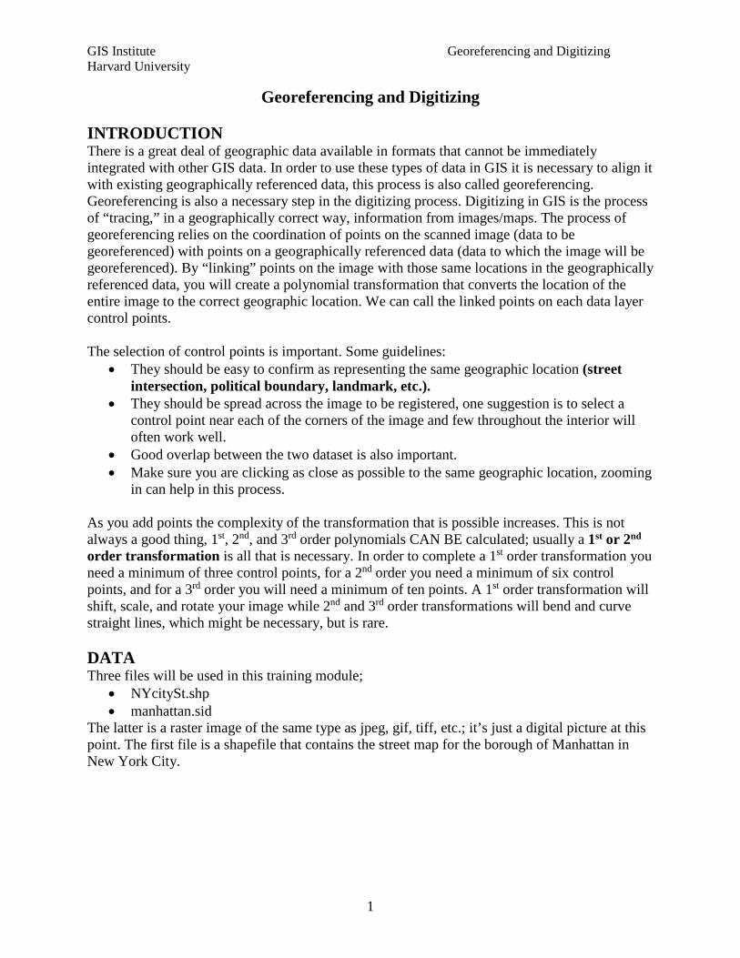
Georeferencing/Registering an Image Tools: The primary tool we will be using is the georeferencing toolbar. The georeferencing toolbar is probably not visible when you first open ArcGIS, you can open it be clicking on customize, selecting toolbars, then clicking on the georeferencing toolbar option. The toolbar should appear in the ArcGIS window.

Figure 1: Georeferencing Toolbar

→ Add both the NYcitySt shapefile and Manhattan image to your ArcMap session. The .sid format holds three subfiles (don’t add them individually), you must select manhattan.sid than then click add.

→ Right click the shapefile (not image) and “Zoom to Layer,” this is a nice feature you might have used before that lets us get to the geographic extent of a specific data layer quickly.

→ From the georeferencing toolbar, if the manhattan.sid file does not appear in the pull-down window nexting “Georeferencing,” click the dropdown arrow and select the manhattan.sid image name.

→ Click “Georeferencing” and select “Fit to Display” from the dropdown.

→ This will display the image in the same general space as the Manhattan census tracts layer.

→ Before adding control points, you should move the image around a bit to get it closer to the orientation and position of the GIS layers you are using. Use the Rotate, Shift, and Scale tools for this. These tools are at the far right of the georeferencing toolbar; the last icon (probably displayed initially as a rotation arrow).

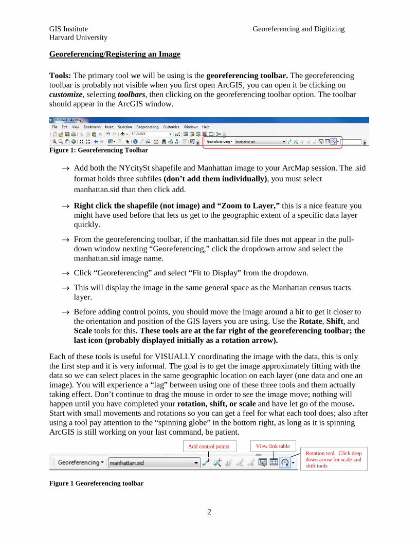
Each of these tools is useful for VISUALLY coordinating the image with the data, this is only the first step and it is very informal. The goal is to get the image approximately fitting with the data so we can select places in the same geographic location on each layer (one data and one an image). You will experience a “lag” between using one of these three tools and them actually taking effect. Don’t continue to drag the mouse in order to see the image move; nothing will happen until you have completed your rotation, shift, or scale and have let go of the mouse. Start with small movements and rotations so you can get a feel for what each tool does; also after using a tool pay attention to the “spinning globe” in the bottom right, as long as it is spinning ArcGIS is still working on your last command, be patient.

Figure 1 Georeferencing toolbar

Rotation tool. Click drop down arrow for scale and shift tools

View link table Add control points


3

→ Now you are ready to add control points (also called link points or links). Click on the

Add Control Points tool.

→ You should be using the street labels to help identify specific streets and intersections for georeferencing. (Right click the layer and select label features).

→ To add a link, click the mouse on the image first, then on a known location on the GIS database. The order of clicking is IMPORTANT. You can use the magnify tools to get a close look at subsets of the data.

→ You can also turn on the effect toolbar to change the transparency to see both layers at once if you like, or you can turn the layers off and one as you select points from each.

→ Once you have added a few links you can open the link table to see how each has worked. View Link Table is the final icon on the right of the georeferencing toolbar.

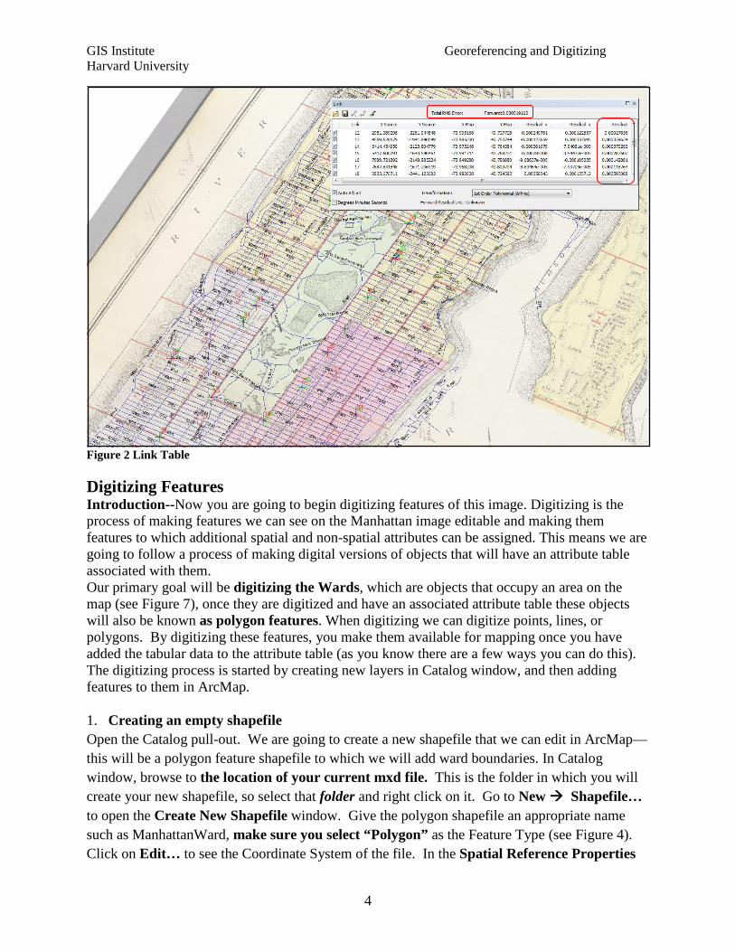
In the link table, you can view the Total RMS Error as well as the Residual for each link that contributes to the overall total (see Figure 3). The errors are associated with the amount of disagreement between the two control points for each link once the transformation is set (once you’ve added more than three links). You have to be sure that the two points that are linked are the same place in world (same street intersection for instance), as you could have a very low error and residuals but not have an accurately registered image, although this is unlikely. In the window, you can also remove links if you think they are in error; when you do this, the registration is automatically recalculated without that pair of points. Before the next step, but after you are happy with your registered image, click save, this will save the data in your link table to a text file that can be opened up in word for later reference. Once you are satisfied with the registration you can Update Georeferencing. This is an option in the georeferencing toolbox, just click on the word georeferencing and a pull down menu will appear with “update georeferencing” as the first option. This will save your transformation. This process will add an .aux file that contains information about the transformation that is necessary to view this file in the future with other data. Don’t forget to save your work, save your map as “xxx”.mxd.


4

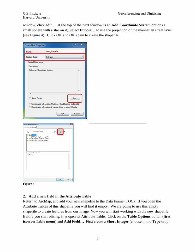
Figure 2 Link Table Digitizing Features Introduction--Now you are going to begin digitizing features of this image. Digitizing is the process of making features we can see on the Manhattan image editable and making them features to which additional spatial and non-spatial attributes can be assigned. This means we are going to follow a process of making digital versions of objects that will have an attribute table associated with them. Our primary goal will be digitizing the Wards, which are objects that occupy an area on the map (see Figure 7), once they are digitized and have an associated attribute table these objects will also be known as polygon features. When digitizing we can digitize points, lines, or polygons. By digitizing these features, you make them available for mapping once you have added the tabular data to the attribute table (as you know there are a few ways you can do this). The digitizing process is started by creating new layers in Catalog window, and then adding features to them in ArcMap. 1. Creating an empty shapefile Open the Catalog pull-out. We are going to create a new shapefile that we can edit in ArcMap—this will be a polygon feature shapefile to which we will add ward boundaries. In Catalog window, browse to the location of your current mxd file. This is the folder in which you will create your new shapefile, so select that folder and right click on it. Go to New Shapefile… to open the Create New Shapefile window. Give the polygon shapefile an appropriate name such as ManhattanWard, make sure you select “Polygon” as the Feature Type (see Figure 4). Click on Edit… to see the Coordinate System of the file. In the Spatial Reference Properties


5

window, click edit…, at the top of the next window is an Add Coordinate System option (a small sphere with a star on it), select Import… to use the projection of the manhattan street layer (see Figure 4). Click OK and OK again to create the shapefile.

Figure 3 2. Add a new field in the Attribute Table Return to ArcMap, and add your new shapefile to the Data Frame (TOC). If you open the Attribute Tables of this shapefile you will find it empty. We are going to use this empty shapefile to create features from our image. Now you will start working with the new shapefile. Before you start editing, first open its Attribute Table. Click on the Table Options button (first icon on Table menu) and Add Field… First create a Short Integer (choose in the Type drop-


6

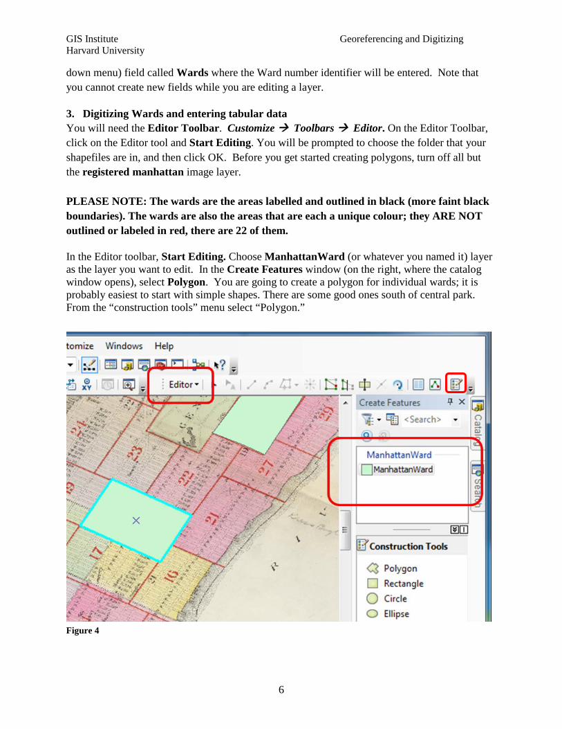
down menu) field called Wards where the Ward number identifier will be entered. Note that you cannot create new fields while you are editing a layer. 3. Digitizing Wards and entering tabular data You will need the Editor Toolbar. Customize Toolbars Editor. On the Editor Toolbar, click on the Editor tool and Start Editing. You will be prompted to choose the folder that your shapefiles are in, and then click OK. Before you get started creating polygons, turn off all but the registered manhattan image layer. PLEASE NOTE: The wards are the areas labelled and outlined in black (more faint black boundaries). The wards are also the areas that are each a unique colour; they ARE NOT outlined or labeled in red, there are 22 of them. In the Editor toolbar, Start Editing. Choose ManhattanWard (or whatever you named it) layer as the layer you want to edit. In the Create Features window (on the right, where the catalog window opens), select Polygon. You are going to create a polygon for individual wards; it is probably easiest to start with simple shapes. There are some good ones south of central park. From the “construction tools” menu select “Polygon.”

Figure 4


7

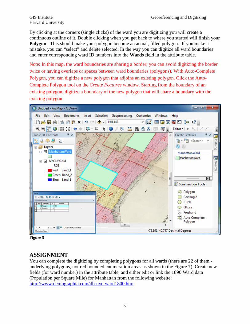
By clicking at the corners (single clicks) of the ward you are digitizing you will create a continuous outline of it. Double clicking when you get back to where you started will finish your Polygon. This should make your polygon become an actual, filled polygon. If you make a mistake, you can “select” and delete selected. In the way you can digitize all ward boundaries and enter corresponding ward ID numbers into the Wards field in the attribute table.

Note: In this map, the ward boundaries are sharing a border; you can avoid digitizing the border twice or having overlaps or spaces between ward boundaries (polygons). With Auto-Complete Polygon, you can digitize a new polygon that adjoins an existing polygon. Click the Auto-Complete Polygon tool on the Create Features window. Starting from the boundary of an existing polygon, digitize a boundary of the new polygon that will share a boundary with the existing polygon.

Figure 5

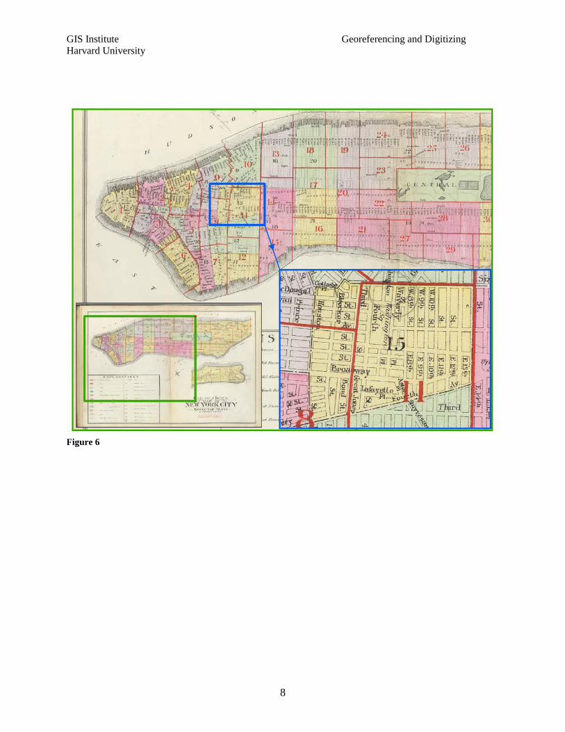
ASSIGNMENT You can complete the digitizing by completing polygons for all wards (there are 22 of them - underlying polygons, not red bounded enumeration areas as shown in the Figure 7). Create new fields (for ward number) in the attribute table, and either edit or link the 1890 Ward data (Population per Square Mile) for Manhattan from the following website: http://www.demographia.com/db-nyc-ward1800.htm

http://www.demographia.com/db-nyc-ward1800.htm


8

Figure 6

georeferencing and digitizing introduction · 1 . georeferencing and digitizing . introduction ....

Documents