1 | P a g e

Geophysical and Topographical Survey

Report

Oldbury Camp, Oldbury-on-Severn

Mary Lennox

David Lambie

with contributions from John Poole

18th February 2017

Jeff Sargent

2 | P a g e

Contents 1. Summary ............................................................................................................................... 4

2. Acknowledgements ............................................................................................................... 4

3. Introduction ........................................................................................................................... 5

3.1. Site references ....................................................................................................................... 5

3.2. Aims and objectives ............................................................................................................... 5

3.3. Report overview .................................................................................................................... 5

3.4. Description of the monument ............................................................................................... 6

3.5. Historical references ............................................................................................................. 9

3.6. Mapping and name ............................................................................................................... 9

4. Methods .............................................................................................................................. 13

4.1. Gradiometry ........................................................................................................................ 13

4.2. Earth resistance ................................................................................................................... 13

4.3. Topographical survey .......................................................................................................... 14

5. Geophysical survey results .................................................................................................. 14

5.1. Field 1 .................................................................................................................................. 14

5.2. Field 2 .................................................................................................................................. 17

5.3. Field 3 .................................................................................................................................. 20

5.4. Fields 4 and 5 ....................................................................................................................... 24

5.4.1. Fields 4 and 5 – Earlier field layout ..................................................................................... 24

5.4.2. Field 4 survey ....................................................................................................................... 25

5.4.3. Field 5 survey ....................................................................................................................... 27

5.5. Field 6 .................................................................................................................................. 30

6. Topographical survey results............................................................................................... 32

7. Conclusion and suggestions for future work ....................................................................... 33

8. References ........................................................................................................................... 35

9. Appendix 1 - Historical Google images ................................................................................ 37

10. Appendix 2 - dGPS reference points ................................................................................... 39

11. Appendix 3 - Geophysics analysis histories ......................................................................... 41

12. Appendix 4 - Raw measurements ....................................................................................... 43

3 | P a g e

Figures 1. Showing Oldbury-on-Severn in southern England

2. Showing Oldbury-on Severn in reference to Thornbury

3. Showing the Toot

4. Extent of scheduled area on monument

5. Lidar heights around the monument

6. Overview of site

7. Extract from “Beauties of England and Wales map 1805 showing two camps

8. Tithe map of around 1840

9. 2nd edition 25”OS mapping

10. 3rd Edition 25” OS mapping

11. Modern mapping

12. Second Tithe Map

13. Field 1 survey results

14. Field 2 survey results

15. Lidar image from QGIS showing section of Field 3 topography

16. Overlay of modern boundaries on tithe map for Field 3

17. Field 3 survey results

18. Second Tithe Map detailed view of Fields 4 and 5

19. Field 4 survey results

20. Field 5 survey results

21. Field 6 survey results

22. Topographic survey results for the Toot

23. Topographic survey results for the Toot - associated notes

24. Locations of test pits based on assessment of geophysics

A2-1. Locations of dGPS datums

4 | P a g e

1. Summary This report summarises the progress to date on non-invasive archaeological

investigations on the Toot, or Camp, at Oldbury-on-Severn, South Gloucestershire,

between December 2015 and December 2016.

The project was supported as part of "A Forgotten Landscape", a Heritage Lottery

Funded Landscape Partnership Scheme.

The aims covered by this report are to perform geophysical and topographical surveys

of the monument; to help focus future excavation work.

Seven of the nine fields on the monument were available for surveying. All of these

seven have been surveyed topographically. Six of them have been surveyed

geophysically.

There was no compelling evidence for any major structures or large-scale man-made

features such as infilled ditches, other than those which are still visible on the surface.

Ephemeral anomalies, particularly resistivity anomalies, were identified as potential

sites for test-pitting. Test pitting results are reported in a separate report from

DigVentures, who supervised the test pitting.

2. Acknowledgements Help for this project has come from many places and is in all cases gratefully received:-

Access to, and permission to survey, the monument has been graciously given the

local landowners, tenants and the community of Oldbury-on-Severn. Their kind

support and assistance was welcome.

Permissions to investigate this scheduled monument were provided by Historic

England.

Funding for this project was provided by the Heritage Lottery Fund, South

Gloucestershire Council and Horizon Nuclear Power.

Archaeological support and practical project management has been provided by the

South Gloucestershire Council. Rebecca Bennett as Project Manager has been

particularly energetic in providing technical and managerial help.

The data gathering and analysis was conducted, in all weathers, by the enthusiastic

team of volunteers recruited to this project as part of the “A Forgotten Landscape”

Landscape Partnership Scheme.

Training in geophysical and topographical surveying was provided by Philip Rowe and

Hazel Riley respectively.

Local historical experience was offered by Jane Bradshaw and Glynn Poole, AFL

volunteers.

The lidar picture used on the title page was produced by Jeff Sargent, AFL volunteer.

All these groups and individuals are thanked for their help and support to the project, all have been

essential to the success of the project.

5 | P a g e

3. Introduction This document summarises the progress to date on archaeological investigations on the Toot, or

Camp, at Oldbury-on-Severn, South Gloucestershire. The aims, objectives and activities reported

here are a subset of those in the original proposal and represent a status report after the first year

of fieldwork.

3.1. Site references Name Oldbury Camp, Oldbury-on-Severn.

Sometimes referred to as “the Toot” or “Toots”

County South Gloucestershire

Parish Oldbury-on-Severn

Altitude Around 10m above mean sea level

UK grid reference ST 6103 9269

Pastscape ref: 201676

NMR NUMBER: ST 69 SW 1

Historic England List entry Number: 1013187

South Gloucestershire Council HER Number: 1568

3.2. Aims and objectives The aim of the work reported here is to gather as much information as possible about the site via

non-invasive means, to inform an excavation plan for Oldbury camp.

The objectives of the work reported here are

1. Undertake gradiometric survey of as many available fields within and around the camp as

possible

2. Undertake earth resistance survey of as many available fields within and around the camp as

possible

3. Perform topographical survey of remaining earthworks

3.3. Report overview This report covers introductory comments on the site and the results of geophysical and

topographical surveys at the Camp, conducted between December 2015 and December 2016. Key

plots of the raw data, processed data and transcriptions of the features are presented together with

a summary of the conclusions drawn.

6 | P a g e

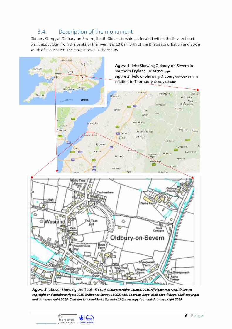
3.4. Description of the monument Oldbury Camp, at Oldbury-on-Severn, South Gloucestershire, is located within the Severn flood

plain, about 1km from the banks of the river. It is 10 km north of the Bristol conurbation and 20km

south of Gloucester. The closest town is Thornbury.

Figure 1 (left) Showing Oldbury-on-Severn in southern England © 2017 Google Figure 2 (below) Showing Oldbury-on-Severn in relation to Thornbury © 2017 Google

Figure 3 (above) Showing the Toot © South Gloucestershire Council, 2015 All rights reserved, © Crown

copyright and database rights 2015 Ordinance Survey 100023410. Contains Royal Mail data ©Royal Mail copyright

and database right 2015. Contains National Statistics data © Crown copyright and database right 2015.

100km 5km

300m 300m

7 | P a g e

Figure 4 Extent of scheduled area on monument

Figure 5 Lidar heights from Red 5m, Blue 13m above mean sea level. The monument lies on a low

rise in the vale. The prominent hill to the south, around 40m high, is topped by St Arilda’s church.

100m

N

8 | P a g e

Figure 6 Overview of site. Red arrows identify the locations where photos were taken and locations

of dGPS traverse across the bi-vallate ramparts and lidar cut though southern height discontinuity Map© South Gloucestershire Council, 2015 All rights reserved, © Crown copyright and database rights 2015 Ordinance Survey 100023410. Contains Royal

Mail data ©Royal Mail copyright and database right 2015. Contains National Statistics data © Crown copyright and database right 2015.

No

rth

3 .

1 .

2 .

Fiel

d 1

Fiel

d 2

Fiel

d 6

Fiel

d 4

Fiel

d 3

Fiel

d 5

Fiel

d 7

Arr

ow

1: V

iew

fro

m c

entr

e o

f b

i-va

llate

ea

rth

wo

rks

sho

win

g in

ner

ear

thw

ork

s o

n le

ft

and

ou

ter

on

th

e ri

ght

Arr

ow

2:

Vie

w d

ow

n C

amp

Ro

ad.

The

inn

er

ear

thw

ork

to

th

e le

ft

rise

s to

th

e in

sid

e o

f th

e

mo

nu

me

nt

Arr

ow

3:

Vie

w o

ver

sou

the

rn f

ield

. Th

e h

ed

ge

con

tain

s a

2 m

ris

e u

p t

o t

he

insi

de

of

the

m

on

um

en

t.

Lid

ar p

rofi

le o

n s

ou

the

rn h

ed

ge.

Dat

a in

me

tre

s go

ing

fro

m s

ou

th

to n

ort

h

dG

PS

dat

a o

n n

ort

he

rn b

i-va

llate

ra

mp

arts

. Arr

ow

mar

ks 2

m

he

igh

t 2

m

Ve

rtic

al s

cale

, he

igh

t ab

ove

me

an

sea

leve

l (m

etr

es)

9 | P a g e

3.5. Historical references

The monument at Oldbury on Severn has long appeared in the historical record. Oldbury-on-Severn

is noted in Camden’s Britannia without reference to the Camp (Camden, 1610). He identified

Oldbury as the "Traiectus" in Antoninus XIV itinerary between Isca to Calleva (Caerleon to

Silchester). In the “Additions and Improvements” of Gibson (Gibson, 1722), the presence of two

camps is noted. One is on the nearby promontory where St Arilda’s church stands in its circular

churchyard, “the Campus minor of the Romans”. The second is taken to be the Toot.

Atkyns (1712) copies Camden, with regard to the camps, while Rudder (1779, p755) expands. Of the

“Campus Major” (the Oldbury Camp) he says

“...part of the intrenchments, with high banks, forming two sides of the square, still remain

pretty perfect, tho’ the other parts are levelled.”

The notable earthworks on the monument today would fit this description from 1779.

Rudder also notes:-

“Just by these, in a piece of ground which still shews many tumps and unevennesses, a great

many foundations have been dug up in the memory of persons living in the place. These

circumstances very much corroborate the opinion that here was the Roman Trajectus, and not

at Aust, as some have fancied.”

It is not clear today what or where these “bumps and unevennesses” were.

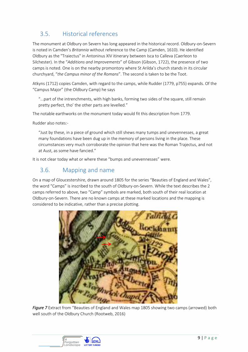
3.6. Mapping and name

On a map of Gloucestershire, drawn around 1805 for the series “Beauties of England and Wales”,

the word “Camps” is inscribed to the south of Oldbury-on-Severn. While the text describes the 2

camps referred to above, two “Camp” symbols are marked, both south of their real location at

Oldbury-on-Severn. There are no known camps at these marked locations and the mapping is

considered to be indicative, rather than a precise plotting.

Figure 7 Extract from “Beauties of England and Wales map 1805 showing two camps (arrowed) both

well south of the Oldbury Church (Rootweb, 2016)

10 | P a g e

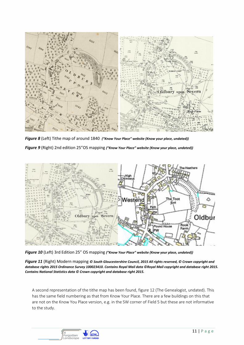
The monument appears in more detailed maps later in the nineteenth century and some examples

from Know Your Place are shown in figures 8 to10 (Knowyourplace, 2016).

An 1840s tithe map shows the principle standing earthworks. The shading looks speculative and

does not represent the slopes of the earthworks.

The monument is present in 1st, 2nd and 3rd edition 25” OS mapping. More of the earthworks are

identified in these maps than in the tithe map including shorter lengths between buildings on the

west. The main earthworks to the north and east are very consistent through this sequence of maps

but the extent of features on the west side reduces in the 3rd edition. In the 1st, 2nd and 3rd editions

of the 25” maps the monument is named “Camp”, “Roman Camp” and finally “The Toot, Camp”,

respectively.

In the 1:50,000 series it is referred to as a “Fort” in 1984 and a “Settlement” in 2011. On the modern

1:25,000 series it is referred to as “The Toot”, and recorded as “Fort”.

Google has recorded a number of images of the monument over the last 17 years. For information

copies of these are presented in Appendix 1.

11 | P a g e

A second representation of the tithe map has been found, figure 12 (The Genealogist, undated). This

has the same field numbering as that from Know Your Place. There are a few buildings on this that

are not on the Know You Place version, e.g. in the SW corner of Field 5 but these are not informative

to the study.

Figure 8 (Left) Tithe map of around 1840 (“Know Your Place” website (Know your place, undated))

Figure 9 (Right) 2nd edition 25”OS mapping (“Know Your Place” website (Know your place, undated))

Figure 10 (Left) 3rd Edition 25” OS mapping (“Know Your Place” website (Know your place, undated))

Figure 11 (Right) Modern mapping © South Gloucestershire Council, 2015 All rights reserved, © Crown copyright and

database rights 2015 Ordinance Survey 100023410. Contains Royal Mail data ©Royal Mail copyright and database right 2015.

Contains National Statistics data © Crown copyright and database right 2015.

12 | P a g e

Figure 12 Second Tithe map (The Genealogist, undated)

N

13 | P a g e

4. Methods The area within the Toot is divided into a series of fields, and access for surveying was granted by

the land owners/occupiers to seven (out of a total of nine) discrete fields, numbered 1 to 7 for

reference (Figure 6). Each field was gridded separately to take best advantage of straight

boundaries, position of obstacles, uneven ground etc. Twenty metre grids were laid out from a

baseline chosen in each field. Surveying tapes were used to measure the grid sizes and ensure the

grids were square. To geolocate the grids, key points on the grids were measured to a network of

datum points laid out using a Differential Global Positioning System (Appendix 2).

The field work was conducted by project volunteers following training in the methods and with

support of more experienced practitioners. Geophysical training was conducted on 14th and 15th

November 2015 and 9th and 10th April 2016, topographical training on 23rd and 30th January

2016.

Details of process are recorded in Appendix 3. The aim throughout all data gathering and the

processing was to be consistent across the entire survey area and to keep processing to the

minimum. The raw data are presented in Appendix 4.

4.1. Gradiometry A gradiometry survey was undertaken over almost the entire survey area (>90%) using a Geoscan

FM 256 fluxgate gradiometer. A standard method was employed in all survey areas; repeated zig-

zag parallel traverses were made at 1 metre traverse intervals and 0.25 metre sample intervals

across each 20 metre grid square. Before each survey session, care was taken to ensure the

gradiometer was allowed to reach equilibrium with air temperature, that it was effectively

balanced to all compass points and vertically, and that it was zeroed in the direction of first

traverse. The settings were regularly checked during each survey session and at each change of

surveyor.

The data (measured in nano-tesla) were logged via the built in data logger, then downloaded to a

laptop after each survey session, before being analysed using Geoplot. A similar method of analysis

was employed across of the six fields which made up the survey area, i.e. assembled into a

composite image for each field and de-spiked or clipped to remove the distorting high magnitude

effects of surface or near surface iron objects. The data were then inspected to identify the

distorting effects of gates, wire fences and other large metal objects and these highly distorting

data were replaced by dummy values (which the software ignores in subsequent analysis). Each

grid was edge-matched to give a uniform visual appearance (zero mean grid) and any stripe errors

removed with zero mean traverse. Finally minimal interpolation was applied in both the x and y

directions to smooth the data slightly for presentation. Every effort was made to keep processing

to a minimum to avoid introducing artificially generated “features”.

4.2. Earth resistance The resistance survey was undertaken using a Geoscan RM15 with multiplexer MPX15 using two

pairs of electrodes each at a 0.5 metre separation. The same grids were used for the resistivity

survey as for the gradiometry, with the traverse interval kept at 1 metre but the sample interval

increased to 0.5 metres. Again, the survey was undertaken in a zig-zag manner, recording the data

in ohms with the inbuilt data logger. As with the gradiometry, data was downloaded to the laptop

and analysed with Geoplot.

14 | P a g e

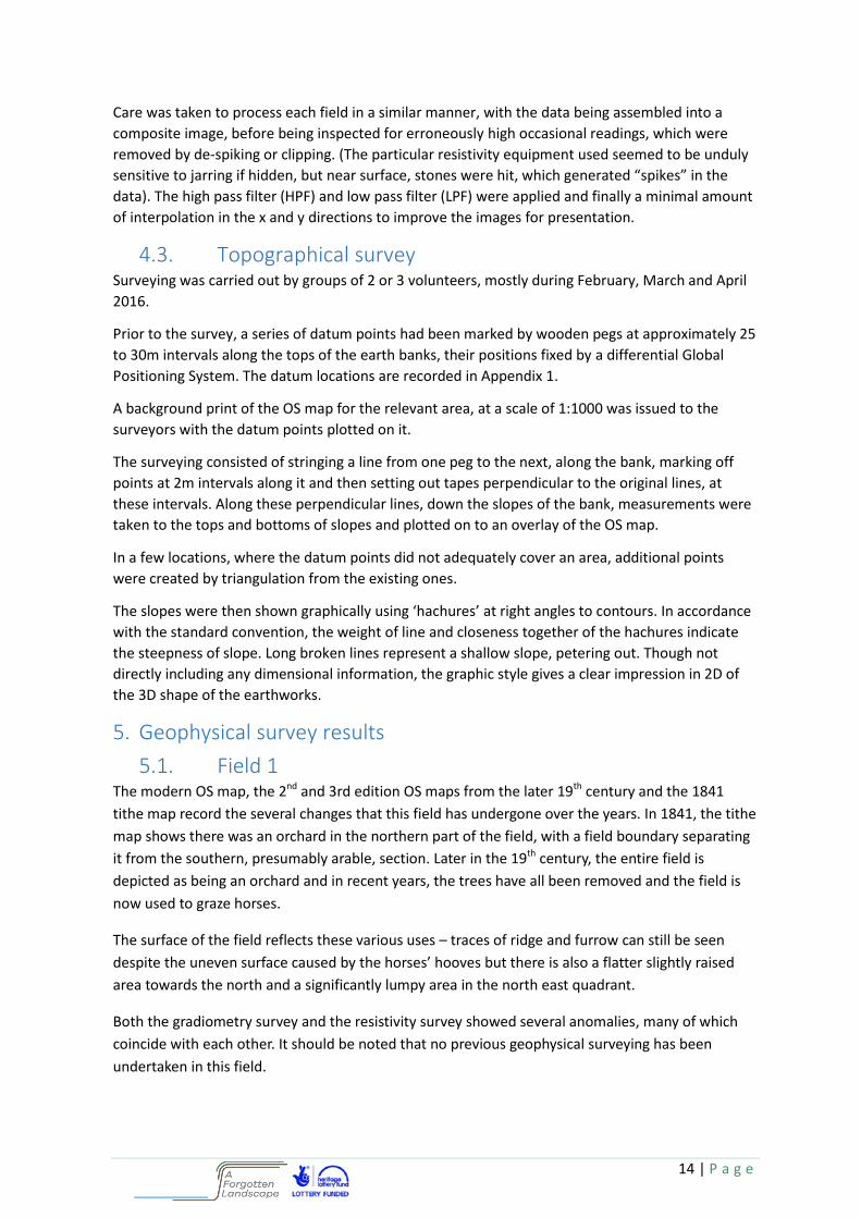
Care was taken to process each field in a similar manner, with the data being assembled into a

composite image, before being inspected for erroneously high occasional readings, which were

removed by de-spiking or clipping. (The particular resistivity equipment used seemed to be unduly

sensitive to jarring if hidden, but near surface, stones were hit, which generated “spikes” in the

data). The high pass filter (HPF) and low pass filter (LPF) were applied and finally a minimal amount

of interpolation in the x and y directions to improve the images for presentation.

4.3. Topographical survey Surveying was carried out by groups of 2 or 3 volunteers, mostly during February, March and April

2016.

Prior to the survey, a series of datum points had been marked by wooden pegs at approximately 25

to 30m intervals along the tops of the earth banks, their positions fixed by a differential Global

Positioning System. The datum locations are recorded in Appendix 1.

A background print of the OS map for the relevant area, at a scale of 1:1000 was issued to the

surveyors with the datum points plotted on it.

The surveying consisted of stringing a line from one peg to the next, along the bank, marking off

points at 2m intervals along it and then setting out tapes perpendicular to the original lines, at

these intervals. Along these perpendicular lines, down the slopes of the bank, measurements were

taken to the tops and bottoms of slopes and plotted on to an overlay of the OS map.

In a few locations, where the datum points did not adequately cover an area, additional points

were created by triangulation from the existing ones.

The slopes were then shown graphically using ‘hachures’ at right angles to contours. In accordance

with the standard convention, the weight of line and closeness together of the hachures indicate

the steepness of slope. Long broken lines represent a shallow slope, petering out. Though not

directly including any dimensional information, the graphic style gives a clear impression in 2D of

the 3D shape of the earthworks.

5. Geophysical survey results

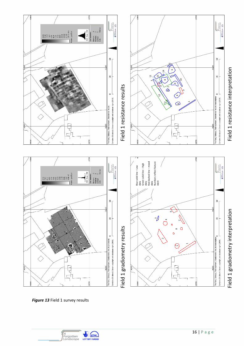
5.1. Field 1 The modern OS map, the 2nd and 3rd edition OS maps from the later 19th century and the 1841

tithe map record the several changes that this field has undergone over the years. In 1841, the tithe

map shows there was an orchard in the northern part of the field, with a field boundary separating

it from the southern, presumably arable, section. Later in the 19th century, the entire field is

depicted as being an orchard and in recent years, the trees have all been removed and the field is

now used to graze horses.

The surface of the field reflects these various uses – traces of ridge and furrow can still be seen

despite the uneven surface caused by the horses’ hooves but there is also a flatter slightly raised

area towards the north and a significantly lumpy area in the north east quadrant.

Both the gradiometry survey and the resistivity survey showed several anomalies, many of which

coincide with each other. It should be noted that no previous geophysical surveying has been

undertaken in this field.

15 | P a g e

Anomaly F1-A: At the west edge of the field, is a narrow northwest to southeast trending linear

feature which seems to be associated with a water tank just north west of the surveyed area. It

exhibits the typical dipole magnetic response (Grad ID 1) of a service pipe and also appears as a low

resistivity anomaly (Res ID 1). This is assumed to be a disused water pipe.

Anomaly F1-B: Towards the north of the field, there is a wide anomaly that was picked up by both

surveys. It appears as an area of magnetic disturbance (Grad ID 2) on the gradiometry survey and as

an area of higher resistivity (Res ID 12) on the resistivity survey. There may also be a T-shaped

higher resistivity anomaly (Res ID 7) associated with it. It appears that this area may correspond to

the old early 19th century boundary and it is suggested that this may represent the footings or the

demolition rubble of a wall that is no longer in existence or the line of an old trackway. The

landowner mentioned that he had done a lot of work to this area to improve drainage; digging out

a ditch and rubble infill.

Anomaly F1-C: Towards the eastern edge of the field, is a rectilinear area of higher resistivity (Res

ID 2) which coincides with a faint circular magnetic anomaly (Grad ID 4, but see also anomalies D

below). There is no indication from the old maps that there was a building in this spot, but it is

possible that the combination of anomalies represents the foundations of a structure which

predates the early 19th century.

Anomalies F-1D: A series of circular low resistance anomalies (Res ID 8) coinciding with magnetic

anomalies (Grad IDs 3 and 4). These may be the result of tree throws from when the old apple trees

were grubbed out.

Anomaly F1-E: A low resistivity anomaly at the eastern edge of the field (Res ID 13) coincides with

the site of a pond which is marked on the old maps, though it no longer exists. There is also a metal

shed in this area which caused a significant magnetic anomaly (Grad ID 5).

Anomaly F1-F: The eastern corner of the field is the permanent site of a dung heap, the run off

from which can be seen in the plume of low resistance readings (Res ID 6). Also in this corner is a

ditch, which results in the low resistivity anomaly (Res ID 5).

Although it hasn’t been specifically identified in the anomaly transcriptions, the resistivity survey

clearly reveals the northwest to south east trending pattern of ridge and furrow which, as

mentioned above, is still clearly visible. Any remaining anomalies are believed to result either from

the wire fences around the field or from metal objects e.g. horseshoes in the ground (Grad IDs 7

and 8) or from rogue resistivity data (Res ID 4).

16 | P a g e

Figure 13 Field 1 survey results

Fiel

d 1

gra

dio

met

ry r

esu

lts

Fiel

d 1

res

ista

nce

res

ult

s

Fiel

d 1

gra

dio

met

ry in

terp

reta

tio

n

Fiel

d 1

res

ista

nce

inte

rpre

tati

on

1

2

3

4 5

6

7 8

Blu

e so

lid li

ne

– Lo

w

dat

a G

ree

n s

olid

lin

e –

Hig

h

dat

a R

ed d

ash

ed li

ne

– m

ixed

d

ata

Nu

mb

ers

refl

ect

feat

ure

id

ent

1

2

3

4

5 6

7

8 8

8

8 8

9 10

11

12

13

14

17 | P a g e

5.2. Field 2 Map evidence from the early 19th Century through to the present day suggests that the boundaries

of this field have remained unchanged. This conclusion is reinforced by the existence of traces of

ridge and furrow which respect the current boundaries.

Today the field is used to graze sheep, but local oral history suggests that the field was used as a

football and cricket pitch for much of the twentieth century. In fact, a set of goal posts still remains

stored in the field edge and they can be seen on a Google Earth air photo from 2005. At that date,

the pitch was smaller than full size – the geophysics detailed below locates the earlier full-sized

pitch.

It is noted that gradiometry and resistivity surveys were undertaken by Roberts (Roberts, 2008)

within this field in 2008, though neither survey covered the entire field.

Anomaly F2-A: The only significant anomaly revealed by the gradiometry survey is a series of strong

dipoles in a rectilinear pattern situated equidistant from each of the field boundaries (Grad ID 1).

This anomaly is also evident in the resistivity survey (Res ID 4) and in view of its size (approximately

20m x 40m) and its location, it is confidently assumed to be the site of the 19th/early 20th century

fenced area which surrounded the cricket wickets, probably to protect the bowling and batting

areas from stock which were grazed in the field outside of the cricket season. The trace on the

resistivity survey will result from liming of the pitch to improve the grass and from the use of lime

to mark out the creases etc.

Anomaly F2-B: The outline of the old football pitch can be clearly seen as a low resistivity anomaly

(for a sample transcribed area, see Res ID 1). There is no trace of the markings visible on the ground

today nor on air photos taken over the last 15+ years but it is believed that lime used to mark out

the pitch persists in the soil in sufficient concentrations to affect the resistivity of the soil.

Anomaly F2-C: These small low resistivity anomalies (Res ID 6, 7 and 8) lie between the field

gateway closest to the road and the football pitch and may be the remains of lime “dumps”, left

behind from the marking out of the pitch.

Anomaly F2-D: Inspection of the resistivity survey plot reveals a series of north/south trending

higher and lower linear anomalies across the majority of the field, particularly on the section away

from the football pitch area. (A sample area is shown on the anomaly transcription as Res ID 3).

These are the geophysical traces of the ridge and furrow which can still be clearly seen on the

ground.

Anomaly F2-E: A faint sub-circular/oval resistivity anomaly (Res ID 5) approximately 10 m along its

east-west axis and possibly 7 or 8 m across its north-south axis can be identified at the eastern edge

of the field. Though the anomaly is very faint and does not appear on the gradiometry survey, it

was also detected by Roberts in 2008 (Roberts, 2008) and so is assumed to be a genuine anomaly. It

is tentatively identified in this report as the trace of a feature such as an animal pen or other light-

weight structure.

Anomaly F2-F: clearly visible along the western side of the field , and possibly extending some

considerable distance (50 metres) eastwards into the field is a “honeycomb” or grid pattern of high

18 | P a g e

resistivity features (Res IDs 2, 10, 11 and 12). The anomaly is not apparent on the gradiometry

survey which unfortunately was quite significantly affected at the field edges by the barbed wire

fencing, such that up to 5 m of the gradiometry date had to be replaced by dummy values and the

remaining data was not entirely outside the zone of influence of the fence. Also unfortunately,

access to the adjacent field to the west was unavailable, so the westward extent of the anomaly has

not been determined. Two possible interpretations present themselves – firstly that the anomaly

results from natural geological features and secondly that it represents an area of habitation or

animal enclosures.

Anomaly F2-G: Trending across the entire field from north-west to south-east is a zone of lower

resistivity (Res ID 9), which widens from less than 20m at the northern end to approximately 30 m

at the southern end. This anomaly is more clearly visible on the raw data plot (see Appendix

1).Although there are field gates in the north-west and south-east corners of the field, and a

footpath crosses the field along this line, the anomaly seems to be too wide and too sharp-edged

to result from farm vehicle or stock movements or from walkers. However it may represent some

agricultural intervention (e.g. liming, aeriation, scarifying etc.) to reduce compaction of the soil in

what is a heavily used field which is prone to waterlogging.

19 | P a g e

Figure 14 Field 2 survey results

Fiel

d 2

gra

dio

met

ry r

esu

lts

Fiel

d 2

res

ista

nce

res

ult

s

Fiel

d 2

gra

dio

met

ry in

terp

reta

tio

n

Fiel

d 2

res

ista

nce

inte

rpre

tati

on

Blu

e so

lid li

ne

– Lo

w

dat

a G

ree

n s

olid

lin

e –

Hig

h

dat

a R

ed d

ash

ed li

ne

– m

ixed

d

ata

Nu

mb

ers

refl

ect

feat

ure

id

ent

1

1

1

3

4

5

6 7 8

2

9

10

11

12

20 | P a g e

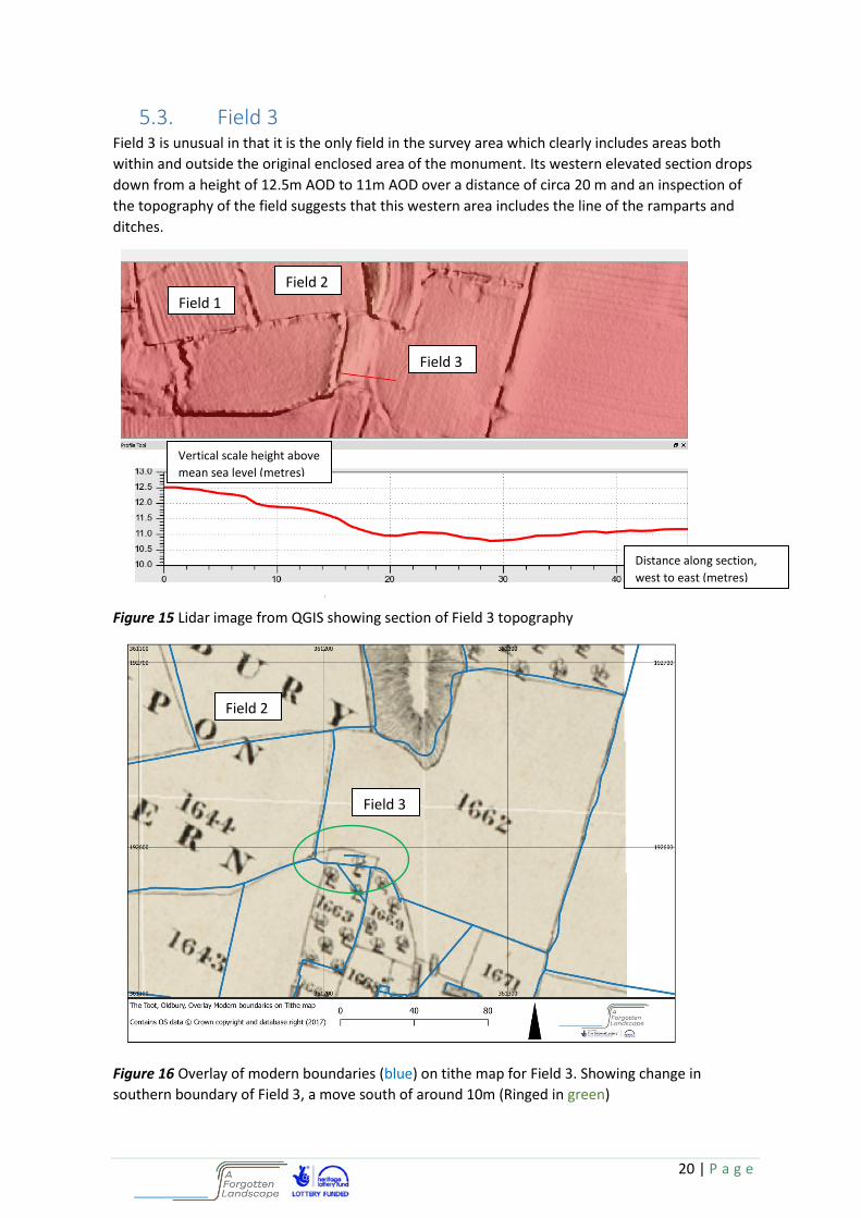
5.3. Field 3 Field 3 is unusual in that it is the only field in the survey area which clearly includes areas both

within and outside the original enclosed area of the monument. Its western elevated section drops

down from a height of 12.5m AOD to 11m AOD over a distance of circa 20 m and an inspection of

the topography of the field suggests that this western area includes the line of the ramparts and

ditches.

Figure 15 Lidar image from QGIS showing section of Field 3 topography

Figure 16 Overlay of modern boundaries (blue) on tithe map for Field 3. Showing change in

southern boundary of Field 3, a move south of around 10m (Ringed in green)

Field 3

Field 2

Field 1

Vertical scale height above

mean sea level (metres)

Distance along section,

west to east (metres)

Field 2

Field 3

21 | P a g e

The eastern section of the field however widens out to include a large level area which is clearly

outside the ramparts. The maps indicate that the present field boundaries (with some possible

short exceptions) date from at least the early 19th century. It would seem sensible to conclude

however, that at some time prior to the 19th century, this smaller, sloping section of the field would

have been separated from the eastern part by a field boundary. The short exception is a 50 or 60 m

stretch of the west end of the southern boundary which appears, from the Tithe map, to now lie 10

m south of its earlier position, see figure 16. This possible older boundary line is preserved today in

a shallow ditch running from east to west in this part of the field. Unfortunately, it is overgrown

and holds dumped stones, farm equipment, tree branches etc. and could not be accessed for the

geophysics.

Also uniquely for the Toot, there was a named tree in the western section of the field, on the line

of the ramparts. The “Battle Elm” appears on the early editions of the OS maps (1st edition up to at

least 1923), but not on the Tithe map. Today the site of the tree is no more than a slight platform in

the break of slope about 25 metres from the northern field boundary and about the same distance

from the western field boundary.

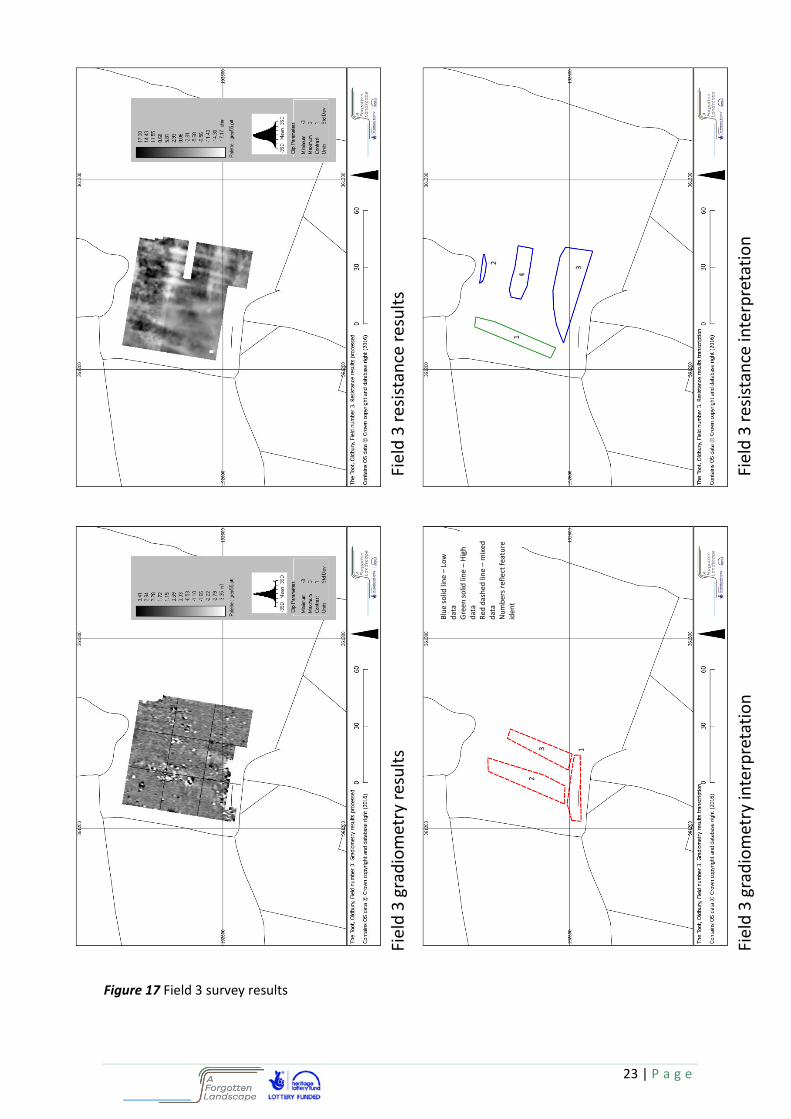
The field is now used as a private light aircraft runway and is also managed for sheep grazing.

Because of weather and stock management issues, both gradiometry and resistivity surveys were

undertaken over two periods; Feb/Mar 2016 and Sept 2016 which resulted in quite significant soil

moisture variation from very wet to very dry. This is most obvious in the resistivity survey, but the

data match quite well and the anomalies continue across the grid edges in a satisfactory manner.

Previously, a gradiometry survey only was undertaken by Roberts (Roberts, 2008) and covered a

very similar area to that described in this report. Roberts concluded that there may once have been

a structure towards the southern area of the survey area.

Anomaly F3-A: One of the clearest anomalies (Grad ID 1) is a broad east-west trending area of

magnetic disturbance which corresponds to the ditch and discarded farm items mentioned above.

No attempt was made to include the whole of this area on the resistivity survey because of the

uneven ground and the difficulty of access.

Anomaly F3-B: A broad northeast/southwest trending area of magnetic disturbance (Grad ID 2)

marks the break of slope at the top of the bank and also incorporates the site of the Battle Elm. The

circular magnetic anomaly visible within the broad anomaly both on the raw and processed data

(but not separately transcribed) may represent the site of the Battle Elm. With the exception of the

possible tree throw, the resistivity survey picks up little sign of the top of the bank.

Anomaly F3-C: A parallel broad northeast/southwest trending anomaly (Grad ID 3) marks the lower

break of slope at the foot of the bank. Again it cannot be seen with any certainty on the resistivity

survey.

Anomaly F3-D: The resistivity survey does pick up with great clarity the traces of the north/south

running ridges and furrows. Unsurprisingly, they occupy the flatter eastern part of the survey area

and are particularly evident where they cross the line of the runway. The runway surface has been

smoothed but the subsurface differences must remain. The lidar results in figure 15 show the lines

of ridge and furrow clearly.

The current survey does not provide any evidence to support Roberts’ contention that there may

have been a structure in this area (Roberts, 2008). Instead, it is concluded that the recent data

22 | P a g e

suggest the line of the rampart and ditches, the effect of the removal of the stump of the Battle

Elm and ridge and furrow are sufficient to account for all the anomalies.

23 | P a g e

Figure 17 Field 3 survey results

Fiel

d 3

gra

dio

met

ry r

esu

lts

Fiel

d 3

res

ista

nce

res

ult

s

Fiel

d 3

gra

dio

met

ry in

terp

reta

tio

n

Fiel

d 3

res

ista

nce

inte

rpre

tati

on

1

2 3

Blu

e so

lid li

ne

– Lo

w

dat

a G

ree

n s

olid

lin

e –

Hig

h

dat

a R

ed d

ash

ed li

ne

– m

ixed

d

ata

Nu

mb

ers

refl

ect

feat

ure

id

ent

4 1

3 2

24 | P a g e

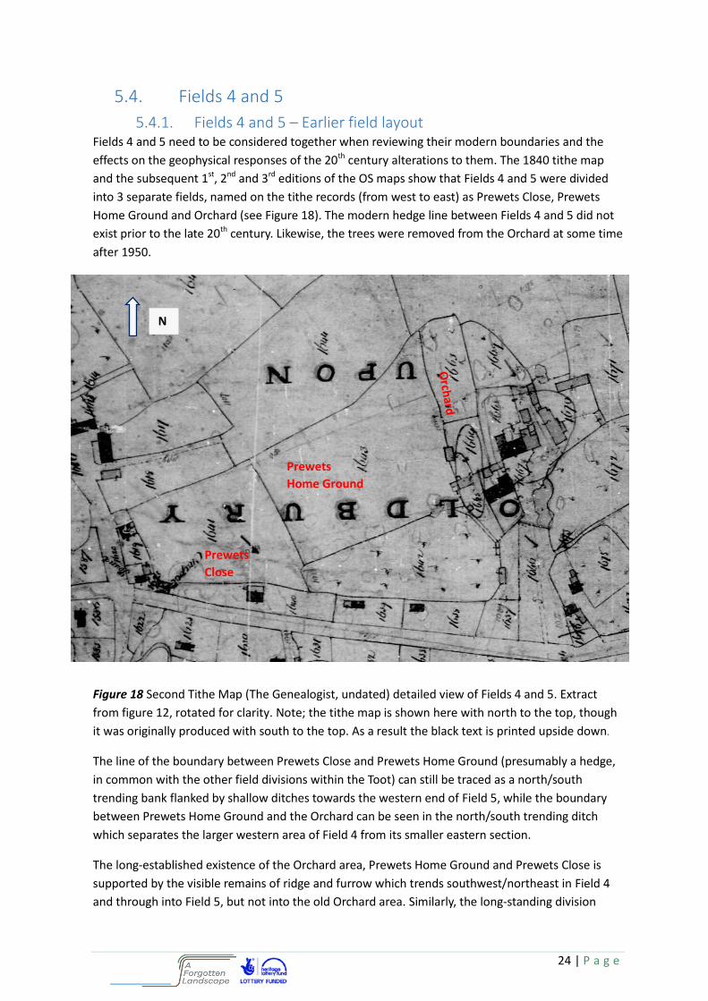
5.4. Fields 4 and 5

5.4.1. Fields 4 and 5 – Earlier field layout Fields 4 and 5 need to be considered together when reviewing their modern boundaries and the

effects on the geophysical responses of the 20th century alterations to them. The 1840 tithe map

and the subsequent 1st, 2nd and 3rd editions of the OS maps show that Fields 4 and 5 were divided

into 3 separate fields, named on the tithe records (from west to east) as Prewets Close, Prewets

Home Ground and Orchard (see Figure 18). The modern hedge line between Fields 4 and 5 did not

exist prior to the late 20th century. Likewise, the trees were removed from the Orchard at some time

after 1950.

Figure 18 Second Tithe Map (The Genealogist, undated) detailed view of Fields 4 and 5. Extract

from figure 12, rotated for clarity. Note; the tithe map is shown here with north to the top, though

it was originally produced with south to the top. As a result the black text is printed upside down.

The line of the boundary between Prewets Close and Prewets Home Ground (presumably a hedge,

in common with the other field divisions within the Toot) can still be traced as a north/south

trending bank flanked by shallow ditches towards the western end of Field 5, while the boundary

between Prewets Home Ground and the Orchard can be seen in the north/south trending ditch

which separates the larger western area of Field 4 from its smaller eastern section.

The long-established existence of the Orchard area, Prewets Home Ground and Prewets Close is

supported by the visible remains of ridge and furrow which trends southwest/northeast in Field 4

and through into Field 5, but not into the old Orchard area. Similarly, the long-standing division

Prewets

Close

Prewets

Home Ground

N

25 | P a g e

between Prewets Close and Prewets Home Ground is confirmed by traces of ridge and furrow at

the western end of Field 5 which run north/south.

The effects of this farming history can be detected in the geophysical survey results as outlined

below.

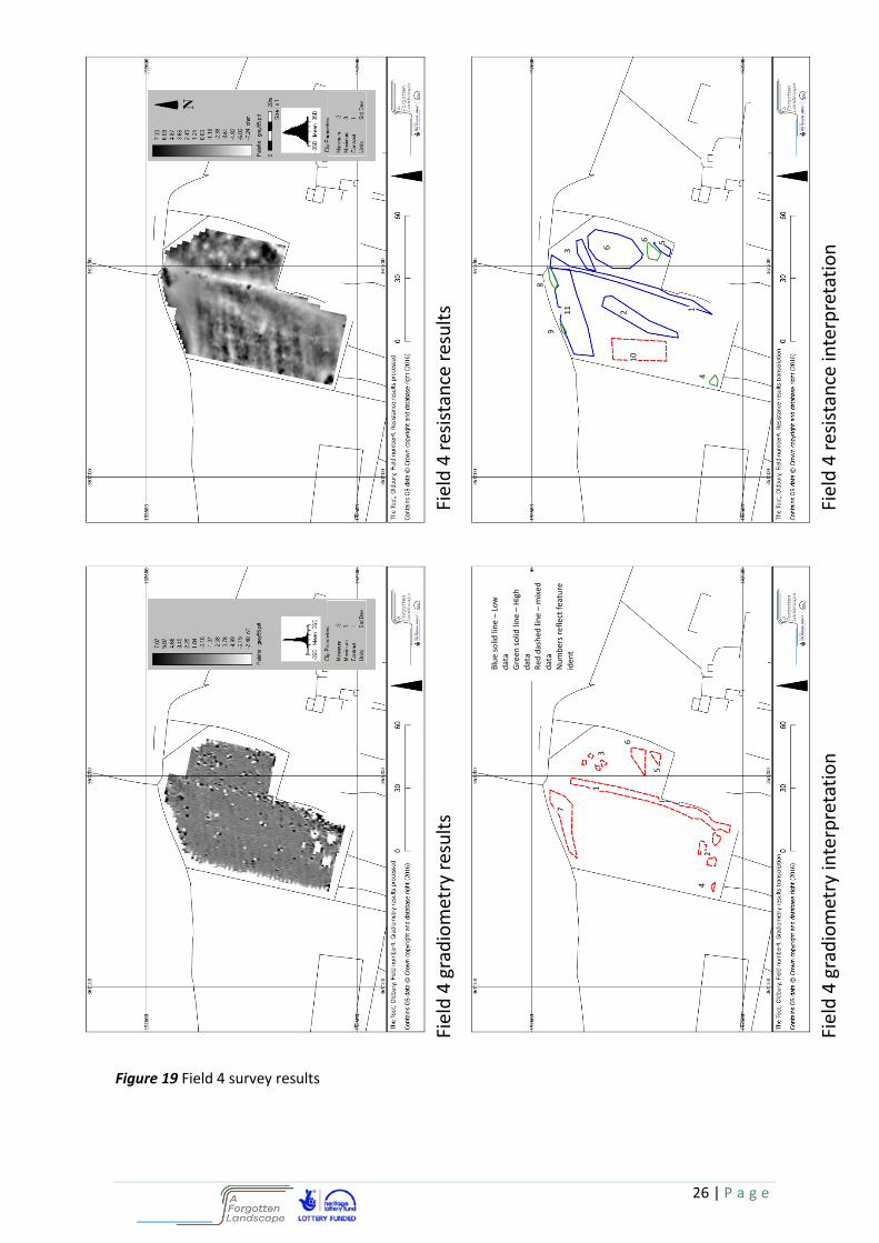
5.4.2. Field 4 survey Anomaly F4-A: The clearest anomaly on both the gradiometry and resistivity surveys (Grad ID 1,

Res ID 1) follows the line of the obvious north/south trending ditch which coincides with the line of

the old field boundary. The southern half of the anomaly seems to continue in a line and without

change of appearance from the northern section, although this section now runs immediately along

the foot of a modern wall and no ditch is visible there. This suggests that the cause of the anomaly

is not related to modern clearing out of the ditch or construction of the wall, and may reflect an

earlier feature.

Anomaly F4-B: Some 5 to 10 metres to the west of Anomaly F4-A is a fainter but more or less

parallel low resistivity anomaly (Res ID 2) which also continues to the southern edge of the field.

There is the possibility that the higher resistivity area between these two anomalies (A and B)

represents the now completely degraded line of the prehistoric bank. Following the line of the

existing banks and ditch across the adjacent Field 3 and south into Field 4 suggest a feasible route

for the prehistoric earthworks towards a possible palaeochannel (See Field 5 results).

Anomaly F4-C: Further west again, approximately 5 metres from anomaly B, lies another fainter low

resistivity anomaly (included in Res ID 2). It is uncertain whether this can also be seen in the

gradiometry data.

Anomaly F4-D: Both the gradiometry and the resistivity surveys show evidence of ridge and furrow

in the western part of the field (Res ID 10), most obviously to the west of anomaly B. If the ridge

and furrow is, for example, medieval, this could suggest that there were some earthworks still

remaining at that date such that ploughing further to the east was not feasible.

Anomaly F4-E: The area of the old orchard displays a very different “texture” on the resistivity

survey compared to the one-time arable area. There are many (six or seven) low resistivity sub-

circular anomalies (Res ID 7) which may represent the tree throws from the removal of the orchard

trees. The ground surface in this area has several circular depressions circa 10 cm in depth which

would tend to confirm the existence of tree throws. The gradiometry survey within this area is

certainly noisier than elsewhere in the field, which again could reflect the ground disturbance due

to the removal of the trees.

Other anomalies identified on the geophysical survey transcriptions have not been specifically

discussed as they are thought to result from modern influences, e.g. the footings for a water

trough, the route of the footpath.

26 | P a g e

Figure 19 Field 4 survey results

Fiel

d 4

gra

dio

met

ry r

esu

lts

Fiel

d 4

res

ista

nce

res

ult

s

Fiel

d 4

gra

dio

met

ry in

terp

reta

tio

n

Fiel

d 4

res

ista

nce

inte

rpre

tati

on

1 2

3

4

5 6

6

8 9

10

11

Blu

e so

lid li

ne

– Lo

w

dat

a G

ree

n s

olid

lin

e –

Hig

h

dat

a R

ed d

ash

ed li

ne

– m

ixed

d

ata

Nu

mb

ers

refl

ect

feat

ure

id

ent

1

2

3

5

7

4

6

27 | P a g e

5.4.3. Field 5 survey Field 5 now has a large (approx. 50m x20m) exercise area for horses which is fenced off from the

rest of the field and surfaced with a thick rubbery material. No geophysics could be undertaken in

this area.

Roberts (2008) reports gradiometry results from part of the field where little variation was seen.

Similarly the results here show very little magnetic variation across the entire field, apart from the

slight traces produced by the ridge and furrow and from the removal of the old boundary between

Prewets Close and Prewets Home Ground. The resistivity survey, however, picked up many more

anomalies.

Anomaly F5-A: The entire southern half of Field 5 shows a different resistivity response from the

northern half (Res ID 14). The resistivity in this area is lower and has a smoother “texture” with

fewer other features than the area to the north. The size of this anomaly, its positioning near the

topographically lower part of the Toot, its smoother texture, and its east/west direction paralleling

the existing rhine all suggest that a palaeochannel may located here. Two other areas within this

possible palaeochannel are an area with a blocky, higher resistivity response which was almost

certainly the result of a heavy rain shower wetting long grass during surveying (Res ID 15) and an

area to the east of the horse exercise arena (Res ID 16) which may be due to construction of the

arena and a trackway (Grad ID 1) which leads into it.

Anomaly F5-B: Dividing the field into two sections is a north/south parallel series of low/high/low

resistance anomalies (Res IDs 3, 4 and 5 and Grad ID 5). This represents the extant bank and

flanking ditches from the old field boundary which can be clearly seen on the ground.

Anomaly F5-C: Running parallel to the ridge and furrow in the eastern part of the field are two low

resistance anomalies (Res ID 6). It is unlikely that these represent any archaeological features and

probably result from raised soil moisture in the remnant furrows after the very wet season prior to

the survey.

Anomaly F5-D: There appears to be a low resistance, rectilinear outline (Res ID 1) with possibly

associated higher resistance areas (Res ID 13) within and beside it and an apparently associated

lower resistance L-shaped feature linking it to the possible palaeochannel feature to the south. The

pronounced right-angle corners within this group of features suggest something man-made though

the remains of building foundations would normally be expected to show a resistance higher than

the background rather than lower. It has been suggested that a robbed out foundation trench

partially backfilled with lime rubble could be responsible for this series of anomalies though it is

noted that there is no map evidence for any structures having been in this spot.

Anomaly F5-E: Immediately to the north of the above series of anomalies is a line of very low

resistance small sub circular anomalies (Res ID 12). It is not clear if these resulted from a data

collection error, but it is noted that the fence line along the entire northern field boundary has been

replaced in recent years (since about 1990) and though they have not been transcribed separately,

there is a line of anomalous resistivity readings along the entire fence line.

Anomaly F5-F: A faint D-shaped lower resistance anomaly (Res IDs 7 and 8) has been identified in

the eastern part of the field close to the arena and the apparent course of the presumed

28 | P a g e

palaeochannel. No explanation other than it possibly being associated with the palaeochannel is

suggested.

29 | P a g e

Figure 20 Field 5 survey results

Fiel

d 5

gra

dio

met

ry r

esu

lts

Fiel

d 5

res

ista

nce

res

ult

s

Fiel

d 5

gra

dio

met

ry in

terp

reta

tio

n

Fiel

d 5

res

ista

nce

inte

rpre

tati

on

1

2

3 4

5

6 7 8

9

12

13

14 15

16

Blu

e so

lid li

ne

– Lo

w

dat

a G

ree

n s

olid

lin

e –

Hig

h

dat

a R

ed d

ash

ed li

ne

– m

ixed

d

ata

Nu

mb

ers

refl

ect

feat

ure

id

ent

1

2

3 4

5

30 | P a g e

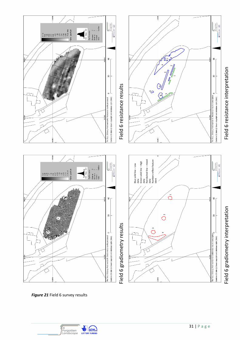
5.5. Field 6 Field 6 is the only field within the geophysical survey area which definitely includes a section of the

prehistoric bank. The entire field rises from south to north such that the northern boundary of the

field follows the top of the inner bank. Originally, the field appears to have extended to the west,

into the area now occupied by cottage gardens. Within living memory, there has been disturbance

of the ground at the 19th century western field boundary as a result of the removal of a hedge line

which edged the footpath.

The tithe map indicates that this field was an orchard in 1840, and was still shown as such on 3rd

edition OS map. Now, however, the field is used to pasture horses and no trees remain.

Anomaly F6-A: The bank bounding the edge of the field shows clearly as an arc of lower resistivity

about 6 or 7 m in width (Res ID 4)

Anomaly F6-B: On the top of the bank, there is a ring of about 6 anomalies of markedly lower

resistance (Res ID 7)

Anomaly F6-C: Within the field are two parallel lower resistance anomalies, each over 40 m in

length and about 5 m apart (Res IDs 1 and 2). It is possible that they reflect an attempt to drain the

field or they may be the trace of ridge and furrow, though there is no visible sign on the ground

surface to support that suggestion.

Anomaly F6-D: Several circular lower resistance anomalies about 5 m in diameter (Res ID 6, 8 and

9) may be tree throws from the removal of orchard trees or (to the west) trees that bounded the

footpath. Similarly, a very low resistance strip adjacent to the western edge of the survey area may

represent the line of the previously enclosed route of the footpath (Res ID 5 and Grad ID 4).

Anomaly F6-E: Three pronounced magnetic dipolar anomalies (Grad ID 1, 2 and 3) seem too

marked to represent archaeological features and are presumed to result from buried modern waste

material such as coils of wire or scraps of corrugated iron sheeting etc.

31 | P a g e

Figure 21 Field 6 survey results

Fiel

d 6

gra

dio

met

ry r

esu

lts

Fiel

d 6

res

ista

nce

res

ult

s

Fiel

d 6

gra

dio

met

ry in

terp

reta

tio

n

Fiel

d 6

res

ista

nce

inte

rpre

tati

on

Blu

e so

lid li

ne

– Lo

w

dat

a G

ree

n s

olid

lin

e –

Hig

h

dat

a R

ed d

ash

ed li

ne

– m

ixed

d

ata

Nu

mb

ers

refl

ect

feat

ure

id

ent

1

2

3

4

1 2

3 4

5

6

7

9 8

32 | P a g e

6. Topographical survey results The main remaining earthworks consist of two banks and a ditch to the north of the village. They

curve to form approximately a quarter circle and lie within Field 7, where most of the survey work

took place, though measurements were also taken in adjacent Fields 2, 3 and 6.

A bank along the east side of Camp Road that appears to be a remnant of the original inner bank

was also surveyed.

Some notes were also made of clues to the previous extent of earthworks where they have been

largely destroyed by development in the medieval and subsequent periods, up to the 1990s.

Camp Road follows the line of the inner ditch and the houses along it have been built on the tops of

both the outer and inner banks. Note was taken of the differences in level between some of the

house floors and the road.

Measurements were taken of the difference in level between Field 5 to the south of the

monument, and the adjacent higher field to the north, which lies within the monument. Access to

this more northerly field was not permitted. This substantial change of level along the hedge line

(up to approximately 1.8m, close to that of the lidar transect) is the southern edge of the

designated monument, though whether it is part of the original perimeter or only marks the edge

of destruction of this part of the monument is not known.

A similar survey of the churchyard of St Arilda’s Church on the nearby hill would be valuable as it

shows indications of being partially an artificial mound.

Figure 22 Topographic survey results for the Toot

33 | P a g e

Figure 23 Topographic survey results for the Toot - associated notes

7. Conclusion and suggestions for future work The aim of this project was to gather information using non-intrusive geophysical and

topographical surveying to identify areas within the Toot as having archaeological potential and to

inform an excavation plan. The topographical survey covered all 7 of the permitted fields (out of a

total of 9 fields within the monument), focusing in particular on the extant sections of banks and

ditches and a plan was produced. The geophysical survey covered 6 out of the 7 fields. Both the

gradiometry and the resistivity surveys yielded data which appeared to be credible, consistent and

indicative of the existence of subsurface features. There was no compelling evidence for any major

structures or large-scale man-made features such as infilled ditches, other than those which are

still visible on the surface. On the other hand, several more ephemeral anomalies, particularly

resistivity anomalies, were identified as potential sites for test-pitting, namely in Fields 1, 2, 3, 5

and 6, as shown in figure 24;

34 | P a g e

Figure 24 Test pit locations (identified by small numerals). These were chosen based on assessment

of the geophysics results.

Test pits were excavated at 9 locations on 5th and 6th November 2016, and the results of the

excavations are detailed in the excavation report (DigVentures, forthcoming).

Suggestions for further work

1) The use of electrical resistance tomography to investigate Field 7, which includes the extant

ditch, but which has not been surveyed to date, due to a combination of steep terrain, very wet

conditions in the base of the ditch and stock management issues. Electrical resistance tomography

could also be used to investigate the area in Field 3 which may include a continuation of the

rampart banks and ditches or a possible entrance of prehistoric date into the interior of the

monument. Finally there is potential for the same technique to further explore the potential

palaeochannel in Field 5.

100m

35 | P a g e

2) The use of standard resistivity surveying at a wider probe spacing to survey at greater depth, in

particular in Field 2 over the “honeycomb” structures.

3) Extension of the topographic survey to the area around the St Arilda’s church to record the

circular boundaries around the church which may have their origins in a prehistoric hilltop

enclosure.

4) Extension of the gradiometry survey to the fields around the church to look for any signs of a

deserted medieval village.

5) Analysis of lidar data covering the area around the Toot and the church to look for indications of

other prehistoric, Roman or early medieval features in the locality which may not have been

previously identified.

6) Environmental sampling of various areas within and immediately outside the Toot, for example,

the “honeycomb” features, the potential palaeochannel and the ditch between the banks, to seek

information for the natural, agricultural and anthropogenic developments to which the monument

has been subjected.

8. References

Atkyns, R. (1712) Ancient and Present State of Glostershire, p590. EP publishing Ltd in collaboration

with Gloucestershire County Library, re-published 1974

Camden, W. (1610) Britain, or, a Chorographical Description of the most flourishing Kingdomes,

England, Scotland, and Ireland. Section GLOCESTERSHIRE. English translation Philemon Holland.

[Online] Source http://www.visionofbritain.org.uk/travellers/Camden/13

(Accessed:- 17th October 2016)

Environment Agency (Undated) https://data.gov.uk/dataset/lidar-tiles-tile-index

(Accessed:- September 2016)

Erskine, JGP. (1990a) ASMR 6383 The Toot, Camp Road, Oldbury-on-Severn Avon

Erskine, JGP. (1990b) ASMR 6419, Land adjoining Cherry Tree Cottage, Camp Road, Oldbury-on-

Severn, Avon Observation and recording of foundation trenches

Franklin, P. (1983) Malaria in Medieval Gloucestershire: an essay in epidemiology. Transactions of the

Bristol and Gloucestershire Archaeological Society no.101 1983 p.115:

Rootweb (2016) http://freepages.genealogy.rootsweb.ancestry.com/~nmfa/Maps/

gloucestershire1805/gloucestershire1805.jpg [online] (Accessed 29th August 2016)

Gibson, E. (1722) Britannia: or a Chorographical Description of Great Britain and Ireland together

with the Adjacent Islands written in Latin by William Camden and translated into English with

Additions and Improvements. London (2nd Edition). Source [Online]

https://ebooks.adelaide.edu.au/c/camden/william/britannia-gibson-1722

(Accessed:- 17th October 2016)

Iles, R. (1980) Excavations at Oldbury Camp, Oldbury-on-Severn, 1978-9 - p35; in Bristol

Archaeological Research Group Review 1, Bristol, pp35-39

Knowyourplace (Undated) http://maps.bristol.gov.uk/kyp/southglos [online]

(Accessed 1st September 2016)

36 | P a g e

Ordnance Survey (2010) A guide to coordinate systems in Great Britain. An introduction to mapping

coordinate systems and the use of GPS datasets with Ordnance Survey mapping. Ordnance Survey

Pastscape (2014) http://www.pastscape.org.uk/hob.aspx?hob_id=201676 [online]

(Accessed 13th April 2016)

Riley, H (2000) Colton Pits, Nettlecombe, Somerset English Heritage, Exeter.

Roberts, AJ. (2008) New Evidence for Viking presence in the Eastern Severn Estuary MSc Dissertation

University of Bristol, Dept. Archaeology and Anthropology

Royal Institution Chartered Surveyors (2010) Guidelines for the use of GNSS in land surveying and

mapping 2nd edn. Royal Institution of Chartered Surveyors, Coventry.

Rudder, S. (1779) A New History of Gloucestershire, p755 Source [online]

https://commons.wikimedia.org/wiki/File:Samuel_Rudder_A_New_History_of_Gloucestershire_177

9.pdf (Accessed:- 12th September 2016)

The Genealogist. (Undated) https://www.thegenealogist.co.uk/ [online] (Accessed Nov 2016)

37 | P a g e

9. Appendix 1 - Historical Google images Google offers a historical perspective on the development of the site recorded below. Dates quotes

are those on the site. Images © www.google.co.uk unless otherwise indicated.

Go

ogl

e su

pp

lied

imag

ing

17

/Ap

r/2

00

5

© 2

01

6 In

fote

rra

Ltd

& B

lues

ky

Go

ogl

e su

pp

lied

imag

ing

7/J

un

/20

05

©

20

16

Info

terr

a Lt

d &

Blu

esky

Go

ogl

e su

pp

lied

imag

ing

31

/Dec

/20

06

©

20

16

Get

map

pin

g p

lc

Go

ogl

e su

pp

lied

imag

ing

31

/Dec

/19

99

©

20

16

Info

terr

a Lt

d &

Blu

esky

38 | P a g e

Go

ogl

e su

pp

lied

imag

ing

31

/Dec

/20

08

©

20

16

Get

map

pin

g p

lc

Go

ogl

e su

pp

lied

imag

ing

14

/Mar

20

13

©

20

16

Dig

ital

Glo

be

Go

ogl

e su

pp

lied

imag

ing

13

/Ju

l/2

01

3

Go

ogl

e su

pp

lied

imag

ing

9/S

ep/2

01

4

39 | P a g e

10. Appendix 2 - dGPS reference points

Figure A2-1 Locations of dGPS datums

Contains OS data © Crown copyright and database right (2016)

Datum locations were set up on the site using a dGPS apparatus by Hazel Riley, a consultant in

landscape history, management and conservation grazing. The survey work was carried out in

January 2016. A network of control points was established across the site using survey grade

differential GPS. The GPS-derived geodetic WGS84 coordinates were transformed to the Ordnance

1

2

3

4

5

6

7

8

9

35

37

34

33

36

38

39

32 3

0

31

29 2

7

28 2

6 25

22

24

23

21

40

20

19

18

17

16

15

14

13

12

11 10

F1

F2

F3

F5

F4

F6

40 | P a g e

Survey National Grid (OSGB36) using the Ordnance Survey’s grid transformation (OSTN02) in Leica’s

GPS post-processing software. Observation times were based on those recommended by the OS

and the RICS in order to obtain accurate height information (OS 2010; RICS 2010).The locations are

plotted above. On the ground they were captured with specific fence posts and wooden pegs. The

actual data are tabulated below. The “Accuracy of Position” quoted in the attributes table for the

background map is 2.5 metres.

dGPS datum points coordinates

Ref Easting Northing Ref Easting Northing

1 360988 192582 21 361145 192820

2 361045 192575 22 361123 192765

3 361079 192576 23 361153 192662

4 361146 192577 24 361134 192657

5 361158 192581 25 361128 192676

6 361198 192593 26 361123 192695

7 361202 192606 27 361117 192714

8 361209 192624 28 361112 192734

9 361223 192651 29 361106 192753

10 361238 192693 30 361100 192754

11 361233 192726 31 361099 192758

12 361265 192708 32 361087 192775

13 361253 192755 33 361042 192779

14 361238 192784 34 361037 192774

15 361220 192806 35 361014 192755

16 361201 192824 36 361056 192773

17 361176 192840 37 361027 192714

18 361212 192751 38 361072 192717

19 361210 192777 39 361089 192727

20 361173 192811 40 361191 192797

41 | P a g e

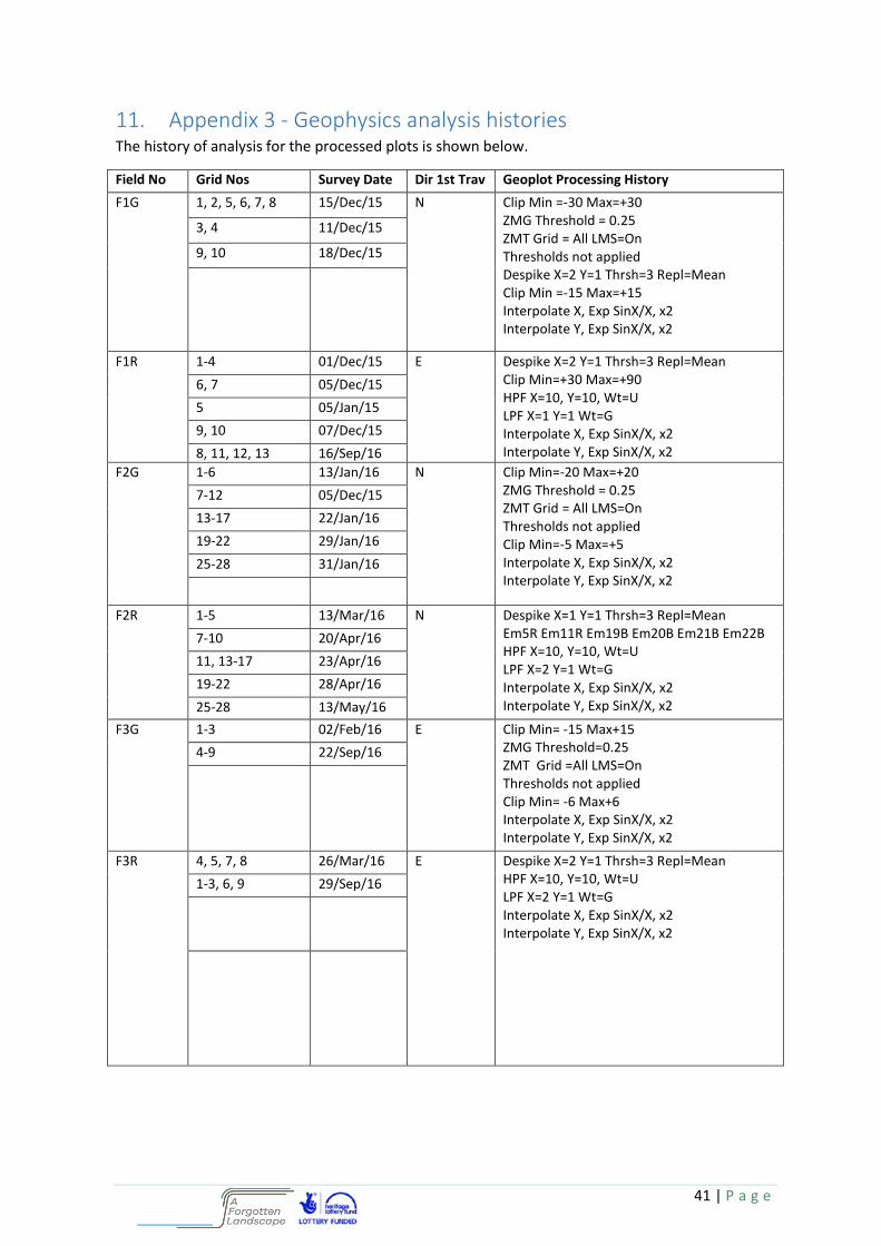
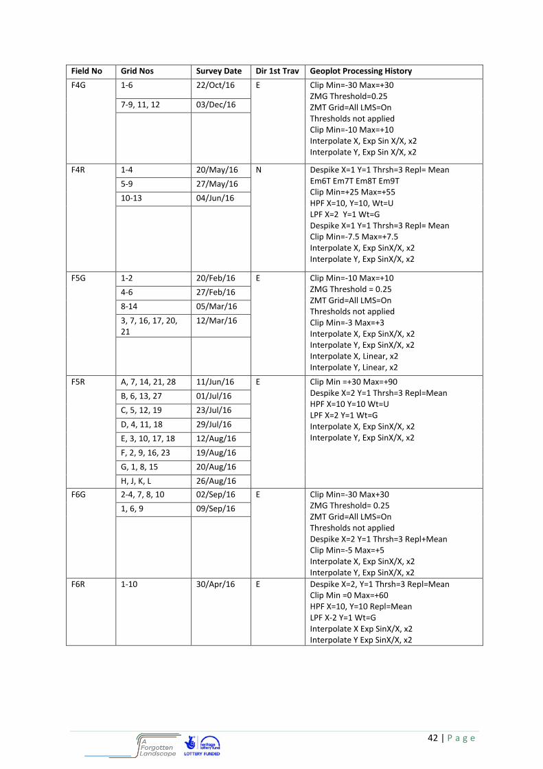
11. Appendix 3 - Geophysics analysis histories The history of analysis for the processed plots is shown below.

Field No Grid Nos Survey Date Dir 1st Trav Geoplot Processing History

F1G 1, 2, 5, 6, 7, 8 15/Dec/15 N Clip Min =-30 Max=+30 ZMG Threshold = 0.25 ZMT Grid = All LMS=On Thresholds not applied Despike X=2 Y=1 Thrsh=3 Repl=Mean Clip Min =-15 Max=+15 Interpolate X, Exp SinX/X, x2 Interpolate Y, Exp SinX/X, x2

3, 4 11/Dec/15

9, 10 18/Dec/15

F1R 1-4 01/Dec/15 E Despike X=2 Y=1 Thrsh=3 Repl=Mean Clip Min=+30 Max=+90 HPF X=10, Y=10, Wt=U LPF X=1 Y=1 Wt=G Interpolate X, Exp SinX/X, x2 Interpolate Y, Exp SinX/X, x2

6, 7 05/Dec/15

5 05/Jan/15

9, 10 07/Dec/15

8, 11, 12, 13 16/Sep/16

F2G 1-6 13/Jan/16 N Clip Min=-20 Max=+20 ZMG Threshold = 0.25 ZMT Grid = All LMS=On Thresholds not applied Clip Min=-5 Max=+5 Interpolate X, Exp SinX/X, x2 Interpolate Y, Exp SinX/X, x2

7-12 05/Dec/15

13-17 22/Jan/16

19-22 29/Jan/16

25-28 31/Jan/16

F2R 1-5 13/Mar/16 N Despike X=1 Y=1 Thrsh=3 Repl=Mean Em5R Em11R Em19B Em20B Em21B Em22B HPF X=10, Y=10, Wt=U LPF X=2 Y=1 Wt=G Interpolate X, Exp SinX/X, x2 Interpolate Y, Exp SinX/X, x2

7-10 20/Apr/16

11, 13-17 23/Apr/16

19-22 28/Apr/16

25-28 13/May/16

F3G 1-3 02/Feb/16 E Clip Min= -15 Max+15 ZMG Threshold=0.25 ZMT Grid =All LMS=On Thresholds not applied Clip Min= -6 Max+6 Interpolate X, Exp SinX/X, x2 Interpolate Y, Exp SinX/X, x2

4-9 22/Sep/16

F3R 4, 5, 7, 8 26/Mar/16 E Despike X=2 Y=1 Thrsh=3 Repl=Mean HPF X=10, Y=10, Wt=U LPF X=2 Y=1 Wt=G Interpolate X, Exp SinX/X, x2 Interpolate Y, Exp SinX/X, x2

1-3, 6, 9 29/Sep/16

42 | P a g e

Field No Grid Nos Survey Date Dir 1st Trav Geoplot Processing History

F4G 1-6 22/Oct/16 E Clip Min=-30 Max=+30 ZMG Threshold=0.25 ZMT Grid=All LMS=On Thresholds not applied Clip Min=-10 Max=+10 Interpolate X, Exp Sin X/X, x2 Interpolate Y, Exp Sin X/X, x2

7-9, 11, 12 03/Dec/16

F4R 1-4 20/May/16 N Despike X=1 Y=1 Thrsh=3 Repl= Mean Em6T Em7T Em8T Em9T Clip Min=+25 Max=+55 HPF X=10, Y=10, Wt=U LPF X=2 Y=1 Wt=G Despike X=1 Y=1 Thrsh=3 Repl= Mean Clip Min=-7.5 Max=+7.5 Interpolate X, Exp SinX/X, x2 Interpolate Y, Exp SinX/X, x2

5-9 27/May/16

10-13 04/Jun/16

F5G 1-2 20/Feb/16 E Clip Min=-10 Max=+10 ZMG Threshold = 0.25 ZMT Grid=All LMS=On Thresholds not applied Clip Min=-3 Max=+3 Interpolate X, Exp SinX/X, x2 Interpolate Y, Exp SinX/X, x2 Interpolate X, Linear, x2 Interpolate Y, Linear, x2

4-6 27/Feb/16

8-14 05/Mar/16

3, 7, 16, 17, 20, 21

12/Mar/16

F5R A, 7, 14, 21, 28 11/Jun/16 E Clip Min =+30 Max=+90 Despike X=2 Y=1 Thrsh=3 Repl=Mean HPF X=10 Y=10 Wt=U LPF X=2 Y=1 Wt=G Interpolate X, Exp SinX/X, x2 Interpolate Y, Exp SinX/X, x2

B, 6, 13, 27 01/Jul/16

C, 5, 12, 19 23/Jul/16

D, 4, 11, 18 29/Jul/16

E, 3, 10, 17, 18 12/Aug/16

F, 2, 9, 16, 23 19/Aug/16

G, 1, 8, 15 20/Aug/16

H, J, K, L 26/Aug/16

F6G 2-4, 7, 8, 10 02/Sep/16 E Clip Min=-30 Max+30 ZMG Threshold= 0.25 ZMT Grid=All LMS=On Thresholds not applied Despike X=2 Y=1 Thrsh=3 Repl+Mean Clip Min=-5 Max=+5 Interpolate X, Exp SinX/X, x2 Interpolate Y, Exp SinX/X, x2

1, 6, 9 09/Sep/16

F6R 1-10 30/Apr/16 E Despike X=2, Y=1 Thrsh=3 Repl=Mean Clip Min =0 Max=+60 HPF X=10, Y=10 Repl=Mean LPF X-2 Y=1 Wt=G Interpolate X Exp SinX/X, x2 Interpolate Y Exp SinX/X, x2

43 | P a g e

12. Appendix 4 - Raw measurements Here the raw measurements of both the resistance and gradiometry surveys, for each field, are

presented for reference. Note the direction arrows on each image give the approximate north.

Fiel

d 1

gra

dio

met

ry r

aw r

esu

lts

Fiel

d 1

res

ista

nce

raw

res

ult

s

Fiel

d 2

gra

dio

met

ry r

aw r

esu

lts

Fiel

d 2

res

ista

nce

raw

res

ult

s

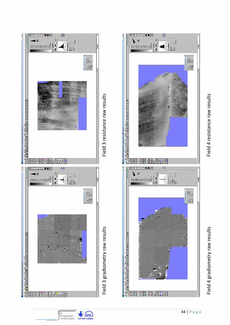
44 | P a g e

Fiel

d 3

gra

dio

met

ry r

aw r

esu

lts

Fiel

d 3

res

ista

nce

raw

res

ult

s

Fiel

d 4

gra

dio

met

ry r

aw r

esu

lts

Fiel

d 4

res

ista

nce

raw

res

ult

s

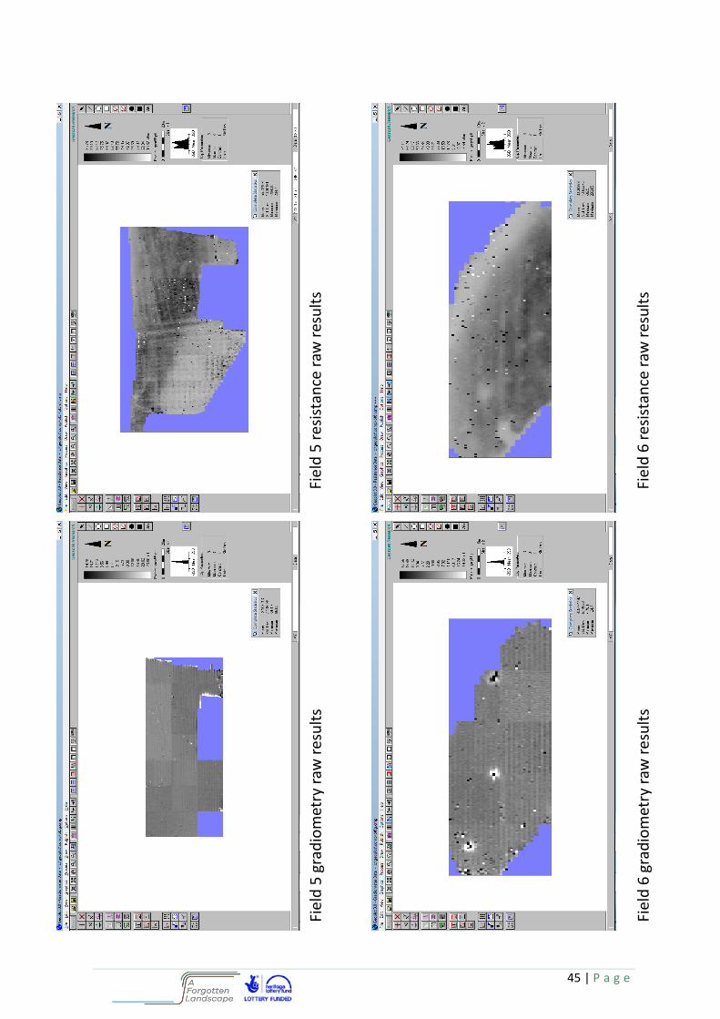
45 | P a g e

Fiel

d 5

gra

dio

met

ry r

aw r

esu

lts

Fiel

d 5

res

ista

nce

raw

res

ult

s

Fiel

d 6

gra

dio

met

ry r

aw r

esu

lts

Fiel

d 6

res

ista

nce

raw

res

ult

s