1

15.053/8 February 12, 2013

Geometry and visualizations of linear programs

© Wikipedia User: 4C. License CC BY-SA. This content is excluded from our CreativeCommons license. For more information, see http://ocw.mit.edu/help/faq-fair-use/.

2

Quotes of the day

“You don't understand anything until you learn it more than one way.”

Marvin Minsky

“One finds limits by pushing them.” Herbert Simon

Overview

Views of linear programming – Geometry/Visualization – Algebra – Economic interpretations

3

What does the feasible region of an LP look like?

4

Three 2-dimensional examples

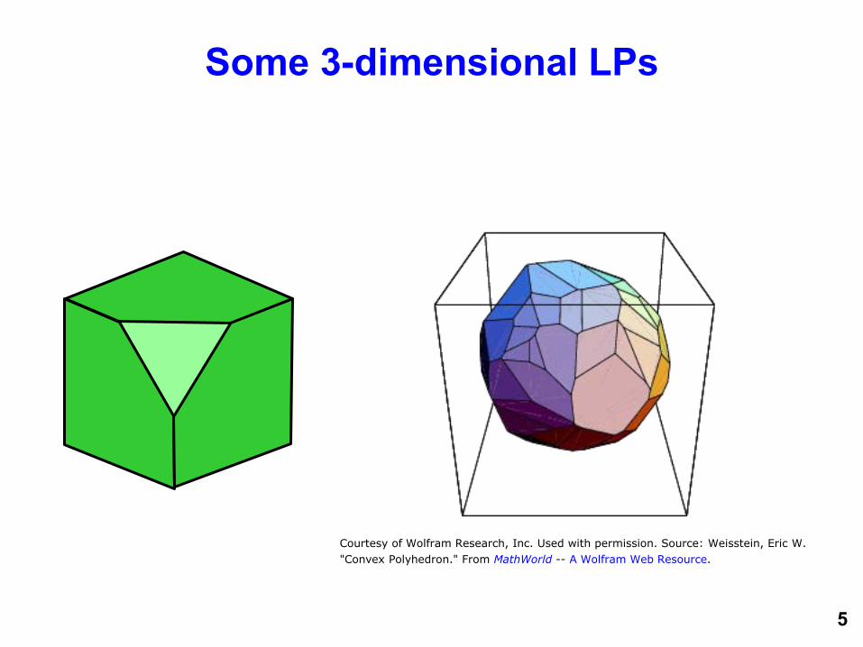
Some 3-dimensional LPs

5

Courtesy of Wolfram Research, Inc. Used with permission. Source: Weisstein, Eric W.

"Convex Polyhedron." From MathWorld -- A Wolfram Web Resource.

6

Goal of this Lecture: visualizing LPs in 2 and 3 dimensions.

What properties does the feasible region have? – convexity – corner points

What properties does an optimal solution have?

How can one find the optimal solution: – the “geometric method” – The simplex method

Introduction to sensitivity analysis – What happens if the RHS changes?

7

A Two Variable Linear Program (a variant of the DTC example)

x, y 0

2x + 3y 10

x + 2y 6

x + y 5

y 3

x 4

z = 3x + 5y objective

(1)

(2)

(3)

(4)

(5)

(6)

Constraints

8

Finding an optimal solution

Introduce yourself to your partner

Try to find an optimal solution to the linear program, without looking ahead.

9

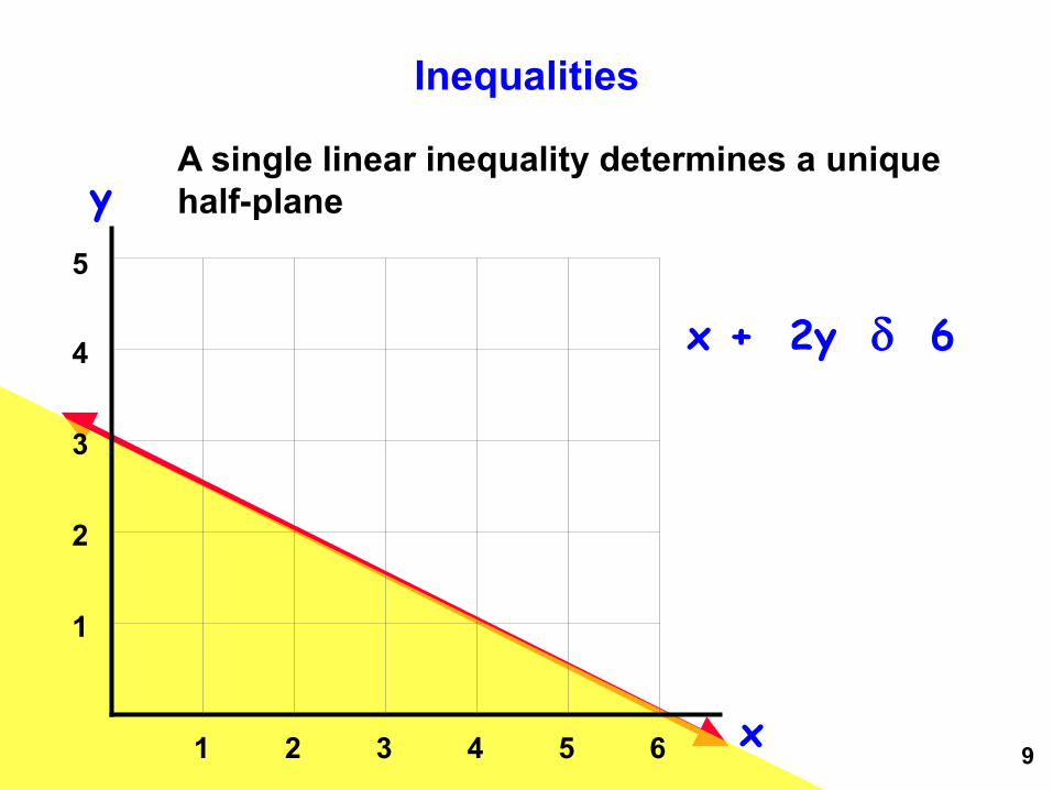
Inequalities

x

y A single linear inequality determines a unique half-plane

x + 2y 6

1 2 3 4 5 6

1

2

3

4

5

1 2 3 4 5 6

1

2

3

4

5

Graph the Constraints:

2x+ 3y 10 (1) x 0 , y 0. (6)

x

y

2x + 3y = 10

Graphing the Feasible Region

10

1 2 3 4 5 6

1

2

3

4

5

Add the Constraint: x + 2y 6 (2)

x

y

x + 2y = 6

11

1 2 3 4 5 6

1

2

3

4

5

Add the Constraint: x + y 5

x

y

x + y = 5

A constraint is called redundant if deleting the constraint does not increase the size of the feasible region.

“x + y = 5” is redundant

12

1 2 3 4 5 6

1

2

3

4

5

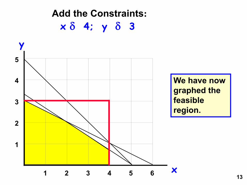
Add the Constraints:

x 4; y 3

x

y

We have now graphed the feasible region.

13

How many constraints are redundant?

14

1. One

2. Two

3. More than two

15

x

y

1 2 3 4

1

2

3

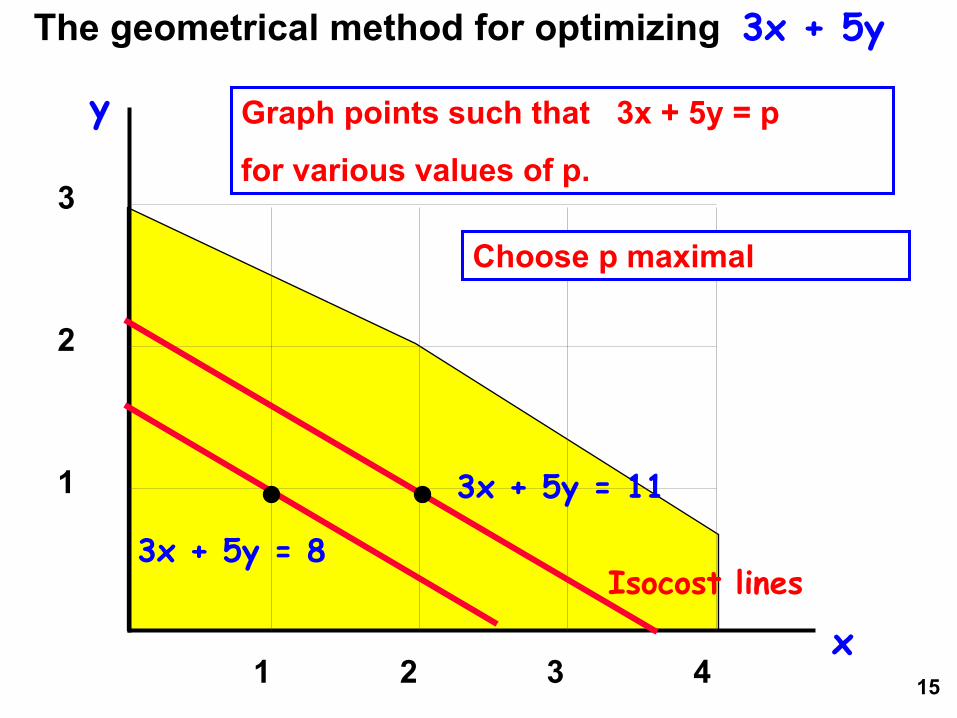
The geometrical method for optimizing 3x + 5y

Graph points such that 3x + 5y = p

for various values of p.

3x + 5y = 11

Choose p maximal

3x + 5y = 8 Isocost lines

16

x

y

1 2 3 4

1

2

3

Find the maximum value p such that there is a feasible solution with 3x + 5y = p.

Move the line with profit p parallel as much as possible.

3x + 5y = 8

3x + 5y = 11

3x + 5y = 16

The optimal solution occurs at a corner point.

Another Problem

17

18

Mental Break

19

Trivia about US

Presidents

20

Different types of LPs

LPs that have an optimal solution.

LPs with unbounded objective. (For a max problem this means unbounded from above.)

Infeasible LP’s: that is, there is no feasible solution.

max x s.t. x + y ≤ -1 x ≥ 0, y ≥ 0

max x s.t. x + y ≤ 1 x ≥ 0, y ≥ 0

max x s.t. x + y ≥ 1 x ≥ 0, y ≥ 0

Try to develop an LP with one or two variables for each of the following three properties.

1. it has no solution 2. it has an optimal solution 3. the solution is unbounded

21

Any other types

Theorem. If the feasible region is non-empty and

bounded, then there is an optimal solution.

This is true when all of the inequalities are “<= constraints”, as opposed to “< constraints”.

e.g., the following problem has no optimum

Maximize x

subject to 0 < x < 1

22 x

y

1 2 3 4

1

2

3

Convex Sets

A set S is convex if for every two points in the set, the line segment joining the points is also in the set; that is,

p1

p2

Theorem. The feasible

region of a linear program is

convex.

if p1, p2 ∈ S, then so is (1 - λ)p1 + λp2 for λ ∈ [0,1].

23 1 2 3 4 5 6

1

2

3

4

5

x

y

not not not not convex convex

More on Convexity

convex Which of the following are ? convex convex or not not ?

© source unknown. All rights reserved. This content is excluded from our CreativeCommons license. For more information, see http://ocw.mit.edu/help/faq-fair-use/.

The feasible region of a linear program is convex

24

x

y

1 2 3 4 5 6

1

2

3

4

5

25

Corner Points

A corner point (also called an extreme point) of the feasible region is a point that is not the midpoint of two other points of the feasible region. (They are only defined for convex sets, to be described later.)

Where are the corner points of this feasible region?

Fact: a feasible LP region has a corner point so long as it does not contain a line.

26

Region 1. No corner point. Feasible region contains a line.

1 2 3 4 5 6

1

2

3

4

5

Region 2. Two corner points. Unbounded feasible region

Region 3.

Facts about corner points.

27

If every variable is non-negative, and if the feasible

region is non-empty, then there is a corner point.

In two dimensions, a corner point is at the intersection of two equality constraints.

Region 2. Two corner points. Unbounded feasible region

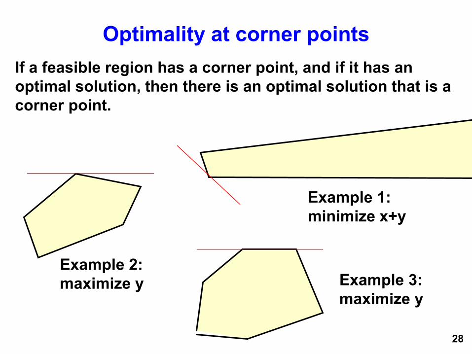
Optimality at corner points

28

If a feasible region has a corner point, and if it has an optimal solution, then there is an optimal solution that is a corner point.

Example 1: minimize x+y

Example 2: maximize y Example 3:

maximize y

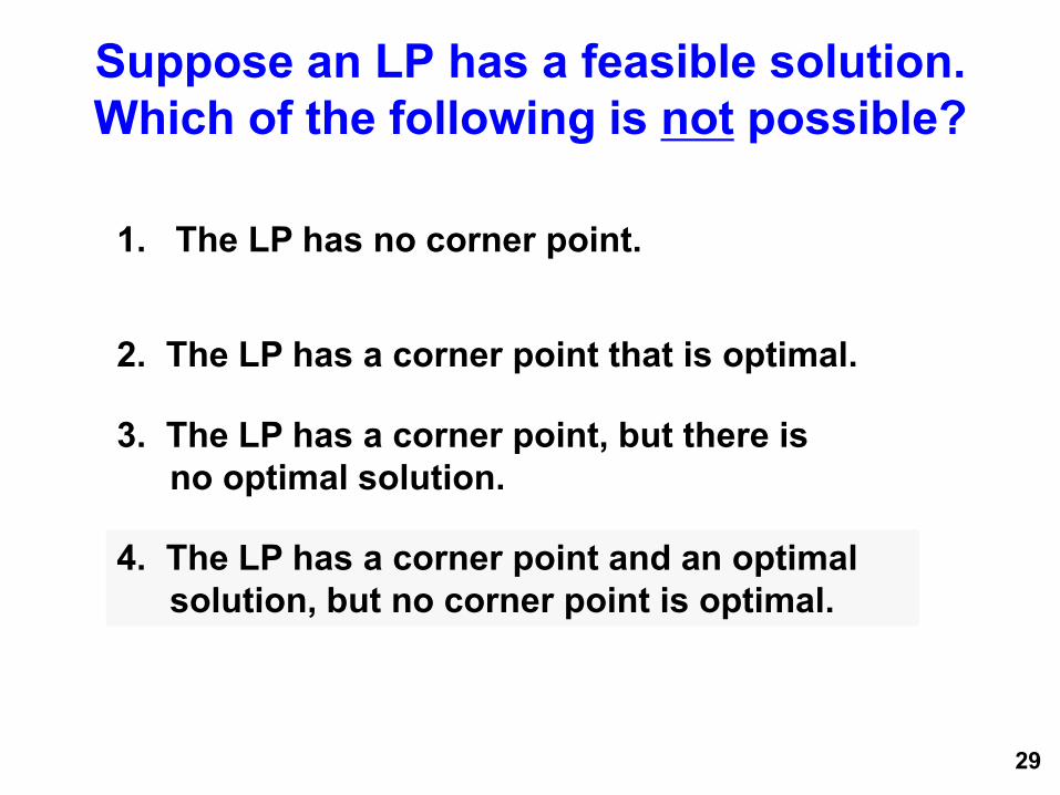
Suppose an LP has a feasible solution. Which of the following is not possible?

29

4. The LP has a corner point and an optimal solution, but no corner point is optimal.

1. The LP has no corner point.

2. The LP has a corner point that is optimal.

3. The LP has a corner point, but there is no optimal solution.

Towards the simplex algorithm

More geometrical notions – edges and rays

Then … the simplex algorithm

30

Edges of the feasible region In two dimensions, an edge of the feasible region

is one of the line segments making up the boundary of the feasible region. The endpoints of an edge are corner points.

31 An edge

In two dimensions, it is a (bounded) equality constraint.

Edges of the feasible region In three dimensions, an edge of the feasible region is

one of the line segments making up the framework of a polyhedron. The edges are where the faces intersect each other. A face is a flat region of the feasible region.

32

A face

A face

An edge

In two dimensions it is a bounded intersection of two equality constraints.

Extreme Rays An extreme ray is like an edge, but it starts

at a corner point and goes on infinitely.

33 x

y

1 2 3 4 5 6

1

2

3

4

5

Two extreme rays.

34

The Simplex Method

34 1 2 3 4 5 6

1

2

3

4

5

x

y

Start at any feasible corner point.

Max z = 3 x + 5 y

3 x + 5 y = 12

35

Is it easy to find a corner point to start at?

In two dimensions it is pretty easy, especially if the LP is already graphed. But with larger LPs, it is surprisingly tricky.

36

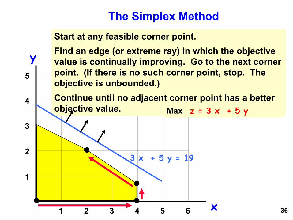
The Simplex Method

1 2 3 4 5 6

1

2

3

4

5

x

y

Start at any feasible corner point. Find an edge (or extreme ray) in which the objective value is continually improving. Go to the next corner point. (If there is no such corner point, stop. The objective is unbounded.) Continue until no adjacent corner point has a better objective value. Max z = 3 x + 5 y

3 x + 5 y = 19

37

The Simplex Method

Pentagonal prism

Note: in three dimensions, the “edges” are the intersections of two constraints. The corner points are the intersection of three constraints.

38

So, one starts at a corner point. At each iteration, one looks for an adjacent corner point that is better. And one stops when there is no improvement.

Does this really work?

Yes. It’s one of the nice (but rare) cases in optimization in which you can find the global optimum by making local improvements.

Cool !! But, the algorithm appears more complicated when there are more variables.

Sensitivity Analysis in 2 Dimensions

39

What happens if the RHS of the constraint 1 decreases from 40?

x = 5 1/3 ; y = 7 1/3 z = 43 1/3

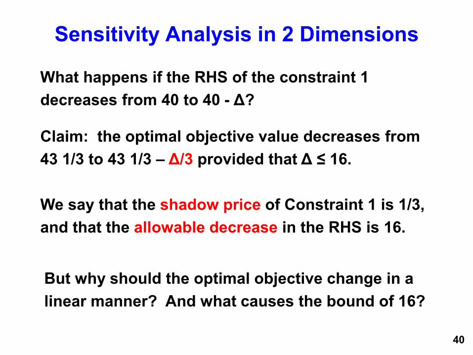
Sensitivity Analysis in 2 Dimensions

40

What happens if the RHS of the constraint 1 decreases from 40 to 40 - Δ?

Claim: the optimal objective value decreases from 43 1/3 to 43 1/3 – Δ/3 provided that Δ ≤ 16. We say that the shadow price of Constraint 1 is 1/3, and that the allowable decrease in the RHS is 16.

But why should the optimal objective change in a linear manner? And what causes the bound of 16?

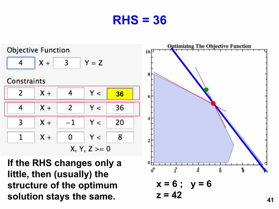
RHS = 36

41

36 36

x = 6 ; y = 6 z = 42

If the RHS changes only a little, then (usually) the structure of the optimum solution stays the same.

RHS = 32

42

32

x = 6 2/3 ; y = 4 2/3 z = 40 2/3

The solution changes, but the structure of the solution stays the same.

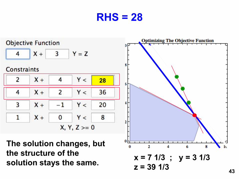
RHS = 28

43

28

x = 7 1/3 ; y = 3 1/3 z = 39 1/3

The solution changes, but the structure of the solution stays the same.

RHS = 24

44

24

x = 8 ; y = 2 z = 38

If we decrease the RHS below 24, then the intersection of the two lines has x > 8, and is infeasible.

Sensitivity Analysis in 2 Dimensions

45

What happens if the RHS of the constraint 1 decreases to 40 - Δ?

4 x + 8 y = 80 - 2Δ

4 x + 2 y = 36 6 y = 44 - 2Δ

y = 7 1/3 – Δ/3

x = (36 -2y)/4 = 5 1/3 + Δ/6

z = 4x + 3y = 43 1/3 - Δ/3

2-Dimensional LPs and Sensitivity Analysis

46

Mita, an MIT Beaver Amit, an MIT Beaver

Hi, we have a tutorial for you stored at the subject web site. We hope to see you there.

It’s on sensitivity analysis in two dimensions. We know that you’ll find it useful for doing the problem set.

47

This concludes geometry and visualization of LPs.

Note for Thursday’s lecture: please review how to solve equations prior to lecture.

Next lecture: the simplex method

MIT OpenCourseWarehttp://ocw.mit.edu

15.053 Optimization Methods in Management ScienceSpring 2013

For information about citing these materials or our Terms of Use, visit: http://ocw.mit.edu/terms.