geometric phase in entangled systems: a single-neutron interferometer experiment
TRANSCRIPT
PHYSICAL REVIEW A 81, 042113 (2010)
Geometric phase in entangled systems: A single-neutron interferometer experiment
S. Sponar,1,* J. Klepp,1 R. Loidl,1 S. Filipp,2 K. Durstberger-Rennhofer,1 R. A. Bertlmann,3 G. Badurek,1
H. Rauch,1,4 and Y. Hasegawa1
1Atominstitut der Osterreichischen Universitaten, A-1020 Vienna, Austria2Department of Physics, Eidgenossische Technische Hochschule Zurich, Schafmattstrasse 16, CH-8093 Zurich, Switzerland
3Faculty of Physics, University of Vienna, Boltzmanngasse 5, A-1090 Vienna, Austria4Institut Laue-Langevin, Boıte Postale 156, F-38042 Grenoble CEDEX 9, France
(Received 28 July 2009; published 30 April 2010)
The influence of the geometric phase on a Bell measurement, as proposed by Bertlmann et al. [Phys. Rev. A69, 032112 (2004)] and expressed by the Clauser-Horne-Shimony-Holt (CHSH) inequality, has been observedfor a spin-path-entangled neutron state in an interferometric setup. It is experimentally demonstrated that theeffect of geometric phase can be balanced by a change in Bell angles. The geometric phase is acquired during atime-dependent interaction with a radiofrequency field. Two schemes, polar and azimuthal adjustment of the Bellangles, are realized and analyzed in detail. The former scheme yields a sinusoidal oscillation of the correlationfunction S, dependent on the geometric phase, such that it varies in the range between 2 and 2
√2 and therefore
always exceeds the boundary value 2 between quantum mechanic and noncontextual theories. The latter schemeresults in a constant, maximal violation of the Bell-like CHSH inequality, where S remains 2
√2 for all settings
of the geometric phase.
DOI: 10.1103/PhysRevA.81.042113 PACS number(s): 03.65.Vf, 03.75.Dg, 03.65.Ud, 07.60.Ly
I. INTRODUCTION
Since the famous 1935 Einstein-Podolsky-Rosen (EPR)gedanken experiment [1], much attention has been devoted toquantum entanglement [2], which is among the most strikingpeculiarities in quantum mechanics. In 1964, J. S. Bell [3]introduced inequalities for certain correlations which holdfor the predictions of any hidden-variable theory applied [4].However, a dedicated experiment was not feasible at thetime. Five years later, Clauser, Horne, Shimony, and Holt(CHSH) reformulated Bell’s inequality pertinent for the firstpractical test of the EPR claim [5]. Thereafter polarizationmeasurements with correlated photon pairs [6], produced byatomic cascade [7,8] and parametric down-conversion of lasers[9–11], demonstrated a violation of the CHSH inequality.To this date, several systems [12–15] have been examined,including neutrons [16].
EPR experiments are designed to test local hidden-variabletheories, thereby exploiting the concept of nonlocality. Localhidden-variable theories are a subset of a larger class ofhidden-variable theories known as the noncontextual hidden-variable theories. Noncontextuality implies that the value ofa measurement is independent of the experimental context,that is, of previous or simultaneous measurements [17,18].Noncontextuality is a less stringent demand than localitybecause it requires mutual independence of the results forcommuting observables even if there is no spacelike separation[19]. First tests of quantum contextuality, based on theKochen-Specker theorem [20], have been recently proposed[21,22] and performed successfully using trapped ions [23] andneutrons [24,25].
In the case of neutrons, entanglement is not achieved be-tween different particles but between different degrees of free-dom. Since the observables of one Hilbert space commute with
observables of a different Hilbert space, the single-neutronsystem is suitable for studying noncontextual hidden-variabletheories. Using neutron interferometry [26,27], single-particleentanglement between the spinor and the spatial part of theneutron wave function [16] and full tomographic state analysis[28] have already been accomplished. In addition, creationof a triply entangled single-neutron state [29] by applying acoherent manipulation method of a neutron’s energy degree offreedom has been demonstrated.
The total phase acquired during an evolution of a quantalsystem generally consists of two components: the usualdynamical phase −1/h
∫H (t)dt , which depends on the
dynamical properties like energy or time, and a geometricphase γ , which is, considering a spin 1/2 system, minushalf the solid angle (�/2) of the curve traced out in rayspace. The peculiarity of this phase, first discovered by Berryin [30], lies in the fact that it does not depend on thedynamics of the system but purely on the evolution path ofthe state in parameter space. From its first verification, forphotons in 1986 [31] and later for neutrons [32], general-izations such as nonadiabatic [33]; noncyclic [34], includingthe Pancharatnam relative phase [35]; off-diagonal evolu-tions [36–38]; and the mixed-state case [39–43] have beenestablished.
The geometric phase in a single-particle system hasbeen studied widely over the past two and a half decades.Nevertheless its effect on entangled quantum systems is lessinvestigated. The geometric phase is an excellent candidate tobe utilized for logic gate operations in quantum communica-tion [44] because of its robustness against noise, which hasbeen tested recently using superconducting qubits [45] andtrapped polarized ultracold neutrons [46]. Entanglement is thebasis for quantum communication and quantum informationprocessing, and therefore studies on systems combing bothquantum phenomena—the geometric phase and quantumentanglement—are of great importance [47–50].
1050-2947/2010/81(4)/042113(10) 042113-1 ©2010 The American Physical Society
S. SPONAR et al. PHYSICAL REVIEW A 81, 042113 (2010)
This article reports on an experimental confirmation forthe violation of Bell-like inequality, relying on correlationsbetween the spin and path degrees of freedom of a single-neutron system under the influence of the geometric phase.The geometric phase is generated in one of the complementaryHilbert spaces, in our case, the spin subspace. We demonstratein detail how the geometric phase affects the Bell anglesettings, required for a violation of a Bell-like inequality inthe CHSH formalism, in a polarized neutron interferometricexperiment. In Sec. II, the theoretical framework, as developedin [48], is briefly described for a spin-path-entangled neutronstate. Expectation values and Bell-like inequalities are definedand the concepts of polar and azimuthal angle adjustmentare introduced. Section III explains the actual measurementprocess. It focuses on experimental issues such as state prepa-ration, manipulation of geometric phase, joint measurements,and the experimental strategy. In the principal part, data analy-sis and experimental results are presented. This is followed bySecs. IV and V, consisting of a discussion and a conclusion.
II. THEORY
A. Expectation values
First we want to clarify the notation since numerousangles are due to appear in this article. Angles denoted asα are associated with path, and angles denoted as β withspin subspace. The prime symbol is used to distinguishdifferent measurement directions of one subspace, required fora CHSH-Bell measurement [5] (e.g., α and α′ represent themeasurement directions for the path subspace). Index 1 denotespolar angles, whereas index 2 is identified with azimuthalangles (e.g., β1 and β ′
1 are polar angles of the spin subspace).Finally, the ⊥ symbol is used for adding π to an angle(e.g., α⊥
1 = α1 + π ).Following the notation given in [48], in our experiment,
the neutron’s wave function is defined in a tensor productof two Hilbert spaces: One Hilbert space is spanned by twopossible paths in the interferometer given by |I〉,|II〉 and theother by spin-up and spin-down eigenstates, denoted as |⇑〉 and|⇓〉, referring to a quantization axis along a static magneticfield. Interacting with a time-dependent magnetic field, theentangled Bell state acquires a geometric phase γ tied to theevolution within the spin subspace [48]:
|�Bell(γ )〉 = 1√2
(|I〉 ⊗ |⇑〉 + |II〉 ⊗ eiγ |⇓〉). (1)
As in common Bell experiments, a joint measurement forspin and path is performed, thereby applying the projectionoperators for the path
Pp±(α) = |± α〉〈±α| (2)
with
|+ α〉 = cosα1
2|I〉 + eiα2 sin
α1
2|II〉,
(3)|− α〉 = − sin
α1
2|I〉 + eiα2 cos
α1
2|II〉,
where α1 denotes the polar angle and α2 the azimuthal angle,and for the spin subspace,
P s±(β) = |± β〉〈±β|, (4)
with
|+ β〉 = cosβ1
2|⇑〉 + eiβ2 sin
β1
2|⇓〉,
(5)|− β〉 = − sin
β1
2|⇑〉 + eiβ2 cos
β1
2|⇓〉.
Introducing the observables
Ap(α) = Pp+(α) − P
p−(α),
(6)Bs(β) = P s
+(β) − P s−(β),
one can define an expectation value for a joint measurementof spin and path along the directions α and β:
E(α,β) = 〈�|Ap(α) ⊗ Bs(β)|�〉= − cos α1 cos β1 − cos(α2 − β2 + γ ) sin α1 sin β1
= − cos(α1 − β1) for (α2 − β2) = −γ. (7)
B. Bell-like inequalities
Next, a Bell-like inequality in a CHSH formalism [5] isintroduced, consisting of four expectation values with theassociated directions α, α′ and β, β ′ for joint measurementsof spin and path, respectively:
S(α,α′,β,β ′,γ ) = |E(α,β)−E(α,β ′) + E(α′,β) + E(α′,β ′)|= |− sin α1[cos(α2 − β2 − γ ) sin β1
− cos(α2 − β ′2 − γ ) sin β ′
1]
− cos α1(cos β1 − cos β ′1)
− sin α′1[cos(α′
2 − β2 − γ ) sin β1
+ cos(α′2 − β ′
2 − γ ) sin β ′1]
− cos α′1(cos β1 + cos β ′
1)|. (8)
The boundary of Eq. (8) is given by the value 2 for anynoncontextual hidden-variable theories [51]. Without loss ofgenerality, one angle can be eliminated by setting, for example,α = 0 (α1 = α2 = 0), which gives
S(α′,β,β ′,γ ) = |− sin α′1[cos(α′
2 − β2 − γ ) sin β1
+ cos(α′2 − β ′
2 − γ ) sin β ′1] − cos α′
1
× (cos β1 + cos β ′1) − cos β1 + cos β ′
1|. (9)
Keeping the polar angles α′1, β1, and β ′
1 constant at theusual Bell angles α′
1 = π/2, β1 = π/4, and β ′1 = 3π/4 (and
azimuthal parts fixed at α′2 = β2 = β ′
2 = 0) reduces S to
S(γ ) = |−√
2 −√
2 cos γ |, (10)
where the familiar maximum value of 2√
2 is reached forγ = 0. For γ = π , the value of S approaches zero.
1. Polar angle adjustment
Here we consider the case when the azimuthal anglesare kept constant, for example, α′
2 = β2 = β ′2 = 0 (α2 = 0),
denoted as
S(α′1,β1,β
′1,γ ) = |− sin α′
1(cos γ sin β1 + cos γ sin β ′1)
− cos α′1(cos β1 + cos β ′
1) − cos β1
+ cos β ′1|. (11)
042113-2
GEOMETRIC PHASE IN ENTANGLED SYSTEMS: A . . . PHYSICAL REVIEW A 81, 042113 (2010)
The polar Bell angles β1, β ′1, and α′
1 (α1 = 0), yielding amaximum S value, can be determined, with respect to thegeometric phase γ , by calculating the partial derivatives (theextremum condition) of S in Eq. (11):
∂S
∂β1= sin β1 + cos α′
1 sin β1 − cos γ sin α′1 cos β1 = 0,
∂S
∂β ′1
= − sin β ′1 + cos α′
1 sin β ′1 − cos γ sin α′
1 cos β ′1 = 0,
∂S
∂α′1
= sin α′1(cos β1 + cos β ′
1)
− cos γ cos α′1(sin β1 + sin β ′
1) = 0. (12)
The solutions are given by
β1 = arctan(cos γ ), (13a)
β ′1 = π − β1, (13b)
α′1 = π
2. (13c)
With these angles, the maximal S decreases for γ : 0 → π/2and touches at γ = π/2 even the limit of the CHSH inequalityS = 2.
2. Azimuthal angle adjustment
Next we discuss the situation where the standard maximalvalue S = 2
√2 can be achieved by keeping the polar angles α′
1,β1, and β ′
1 constant at the Bell angles α′1 = π/2, β1 = π/4,
and β ′1 = 3π/4 (α1 = 0), while the azimuthal parts, α′
2, β2,
and β ′2 (α2 = 0), are varied. The corresponding S function is
denoted as
S(α′2,β2,β
′2,γ ) =
∣∣∣∣∣−√
2 −√
2
2[cos(α′
2 − β2 − γ )
+ cos(α′2 − β ′
2 − γ )]
∣∣∣∣∣ . (14)
The maximum value 2√
2 is reached for
β2 = β ′2, (15a)
α′2 − β ′
2 = γ (mod π ). (15b)
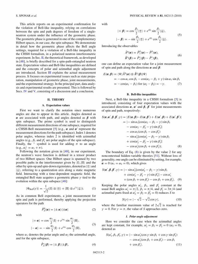
For convenience, β2 = 0 is chosen.The conditions expressed in Eqs. (13a), (13b), and (15b)
(see Bloch spheres in Fig. 1) are experimentally realized usingthe spin turner device and the neutron interferometer (IFM)depicted in Fig. 1.
III. DESCRIPTION OF THE EXPERIMENT
A. State preparation
The preparation of entanglement between spatial and spinordegrees of freedom is achieved by a beam splitter and asubsequent spin-flip process in one subbeam: Behind the beamsplitter (first plate of the IFM), the neutron’s wave function isfound in a coherent superposition of |I〉 and |II〉, and only thespin in |II〉 is flipped by the first radiofrequency (rf) flipperwithin the interferometer (see Fig. 1).
FIG. 1. (Color online) Experimental apparatus for joint measurement of spinor and path degrees of freedom with respect to the geometricphase. The incident neutron beam is polarized by a magnetic field prism. The spin state acquires a geometric phase γ during the interactionwith a rf field within the interferometer. The second rf flipper compensates the energy difference between the two spin components because ofits frequency of ω/2, which is depicted in the energy level diagram of the two interfering subbeams. The accelerator coil is used to eliminatedynamic phase contributions. The beam block is required for measurements solely in one path (±z direction of the path measurement). Finally,the spin is rotated by an angle δ (in the x,z plane) by a dc-spin turner for a polarization analysis and count rate detection. The Bloch-spheredescription includes the measurement settings of α and β(δ), determining the projection operators used for joint measurement of spin and path;α is tuned by a combination of the phase shifter (χ ) and the beam block, and β is adjusted by the angle δ.
042113-3
S. SPONAR et al. PHYSICAL REVIEW A 81, 042113 (2010)
The entangled state that emerges from a coherent superpo-sition of |I〉 and |II〉 is expressed as
|�Bell〉 = 1√2
(|I〉 ⊗ |⇑〉 + |II〉 ⊗ eiωt eiφI |⇓〉), (16)
after the interaction with the oscillating field, given by B(1) =B
(ω)rf cos(ωt + φI) · y. The time-dependent phase ωt is due to
the interaction with the time-dependent magnetic field, wherethe total energy of the neutron is no longer conserved [52–54]since photons of energy hω are exchanged with the rf field(for a more detailed description of the generation of |�Bell〉,see [29]).
B. Manipulation of geometric and dynamical phases
The effect of the first rf flipper, placed inside the interfer-ometer (path II), is described by the unitary operator U (φI),which induces a spinor rotation from |⇑〉 to |⇓〉, denotedas U (φI)|⇑〉 = eiφI |⇓〉. The rotation axis encloses an angleφI with the y direction and is determined by the oscillatingmagnetic field B(1) = B
(ω)rf cos(ωt + φI) · y. Without loss of
generality, one can insert a unity operator, given by 1l =U †(φ0)U (φ0), yielding
U (φI)|⇑〉 =eiγ︷ ︸︸ ︷
U (φI)U†(φ0) U (φ0)|⇑〉︸ ︷︷ ︸
1
= eiγ |⇓〉, (17)
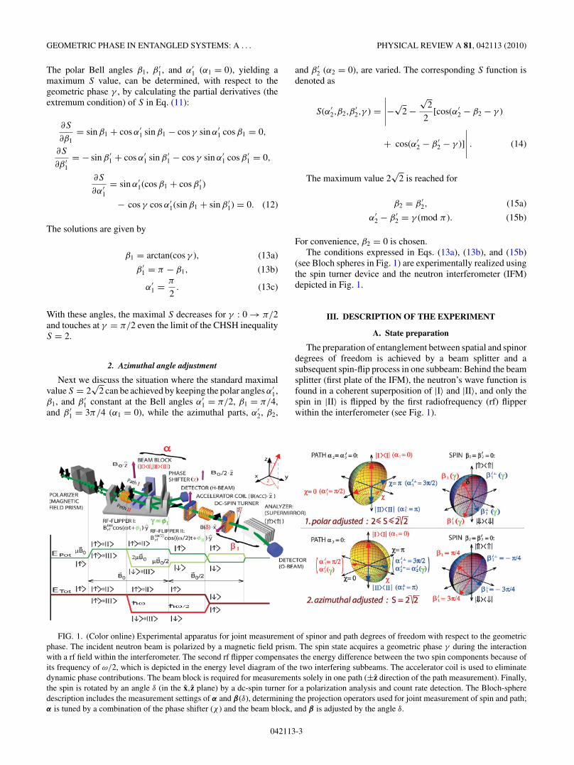
where U (φ0) can be interpreted as a rotation from |⇑〉 to|⇓〉, with the y direction being the rotation axis (φ0 = 0), andU †(φ0) describes a rotation about the same axis back to theinitial state |⇑〉. Consequently, U (φI)U †(φ0) can be identifiedto induce the geometric phase γ along the reversed evolutionpath characterized by φ0 (|⇓〉 to |⇑〉), followed by anotherpath determined by φI (|⇑〉 to |⇓〉). In the rotating frame ofreference [55], the two semigreat circles enclose an angle φI
and the solid angle � = −2φI, yielding a pure geometric phase
γ = −�/2 = φI, (18)
which is depicted in Fig. 2. The entangled state, as describedin [48], is represented by
|�Exp(γ )〉 = 1√2
(|I〉 ⊗ |⇑〉 + |II〉 ⊗ eiωt eiγ |⇓〉), (19)
including the geometric phase γ = φI and a time-dependentdynamic phase ωt . Note that in the last equation, we haveneglected relative phase shifts between path I and II at the beamsplitter (first plate of the IFM) because they can be adjustedreliably with a phase shifter plate inducing a phase factor eiχ
(see Sec. III D for details). In the next step, an experimentalstrategy to cancel the dynamic phase component, by use ofa second rf flipper [29], is utilized: At the last plate of theinterferometer, the two subbeams are recombined, followed byan interaction with the second rf field, with half frequency ω/2denoted as B(1) = B
(ω)rf cos((ω/2)t + φII) · y. The value of φII
was set to zero during the complete experiment. Therefore thespin-down component (spin-up from path I, which is flippedat the second rf flipper) acquires a phase ω/2(t + T ), which is
FIG. 2. (Color online) Bloch sphere representation of the spinorevolution within the first rf flipper, placed inside the interferometer(path II), in the rotating frame of reference. The geometric phase γ
is given by minus half of the solid angle �, traced out by the statevector, depending on the phase φI of the oscillating magnetic field inthe rf flipper.
the same amount but opposite sign of the phase of the spin-upcomponent (path II). The final state is given by
|�Fin(γ )〉 = (|I〉 + |II〉) ⊗ 1√2
[eiω/2(t+T )eiφII |⇓〉
+ eiχeiωt e−iω/2(t+T )ei(γ−φII)|⇑〉]∝ (|I〉 + |II〉) ⊗ 1√
2[eiχei(γ−ωT )|⇑〉 + |⇓〉],
(20)
where ωT is the zero-field phase, with T being the neutron’spropagation time between the two rf flippers and the geometricphase γ = φI. The instants when the neutron is at the centerof the first and second flipper coil are denoted as t and t + T ,respectively. The energy difference between the orthogonalspin components is compensated by choosing a frequency ofω/2 for the second rf flipper, yielding a stationary state vector(see energy level diagram in Fig. 1).
In our experiment, the |⇑〉 eigenstate (in paths I and II) alsoacquires a dynamical phase as it precesses about the magneticguide field in the +z direction. After a spin flip (only in pathII), the |⇓〉 eigenstate still gains another dynamical phase butof opposite sign compared to the situation before the spin flip.The phases of the two guide fields and the zero-field phase ωT
are compensated by an additional Larmor precession within atunable accelerator coil with a static field, pointing in the +zdirection.
An alternative approach toward the generation of thegeometric phase is introduced in Sec. IV, where two rf flippers,one inside and one outside of the interferometer, contribute tothe geometric phase.
042113-4
GEOMETRIC PHASE IN ENTANGLED SYSTEMS: A . . . PHYSICAL REVIEW A 81, 042113 (2010)
C. Joint measurements
Experimentally, the probabilities of joint (projective) mea-surements are proportional to the following count rates,detected after path (α) and spin (β) manipulation:
N++(α,β) = N++[α,(β1,0)] ∝ 〈�Exp(γ )|P p+(α)
⊗P s+(β1,0)|�Exp(γ )〉,
N+−(α,β) = N++[α,(β1 + π,0)] ≡ N++[α,(β⊥1 ,0)]
∝ 〈�Exp(γ )|P p+(α) ⊗ P s
+(β⊥1 ,0)|�Exp(γ )〉,
N−+(α,β) = N++[(α1 + π,α2),(β1,0)]
≡ N++[(α⊥1 ,α2),(β1,0)] ∝ 〈�Exp(γ )|P p
+(α⊥1 ,α2)
⊗P s+(β1,0)|�Exp(γ )〉,
N−−(α,β) = N++[(α⊥1 ,α2),(β⊥
1 ,0)] ∝ 〈�Exp(γ )|P p+(α⊥
1 ,α2)
⊗P s+(β⊥
1 ,0)|�Exp(γ )〉. (21)
The expectation value of a joint measurement of Ap(α) andBs(β),
E(α,β) = 〈�(γ )|Ap(α) ⊗ Bs(β)|�(γ )〉, (22)
is experimentally determined from the count rates
E(α,β)
= N++(α,β) − N+−(α,β) − N−+(α,β) + N−−(α,β)
N++(α,β) + N+−(α,β) + N−+(α,β) + N−−(α,β).
(23)
With these expectation values, S is defined by
S = E(α,β) − E(α,β ′) + E(α′,β) + E(α′,β ′). (24)
D. Experimental setup
The experiment was carried out at the neutron inter-ferometer instrument S18 at the high-flux reactor of theInstitute Laue-Langevin in Grenoble, France. A sketch ofthe setup is depicted in Fig. 1. A monochromatic beam withmean wavelength λ0 = 1.91 A( λ/λ0 ∼ 0.02) and 5 × 5 mm2
beam cross section is polarized by a birefringent magnetic fieldprism in the z direction [56]. Owing to the angular separationat the deflection, the interferometer is adjusted so that onlythe spin-up component fulfills the Bragg condition at the firstinterferometer plate (beam splitter).
As in our previous experiment [29], the spin in path |II〉 isflipped by a rf flipper, which requires two magnetic fields: astatic field B0 · z and a perpendicular oscillating field B(1) =B
(ω)rf cos(ωt + φI) · y with amplitude
B(ω)rf = πh
τ |µ| , ω = 2|µ|B0
h
(1 + B2
1
16B20
), (25)
where µ is the magnetic moment of the neutron and τ denotesthe time the neutron is exposed to the rf field. The second termin ω is due to the Bloch-Siegert shift [57]. The oscillating fieldis produced by a water-cooled rf coil with a length of 2 cm,operating at a frequency of ω/2π = 58 kHz. The static fieldis provided by a uniform magnetic guide field B
(ω)0 ∼ 2 mT,
produced by a pair of water-cooled Helmholtz coils.
The two subbeams are recombined at the third crystalplate where |I〉 and |II〉 only differ by an adjustable phasefactor eiχ (path phase χ is given by χ = −NbcλD, withthe thickness of the phase shifter plate D, the neutronwavelength λ, the coherent scattering length bc, and the particledensity N in the phase shifter plate). By rotating the plate,χ can be varied systematically. This yields the well-knownintensity oscillations of the two beams emerging behind theinterferometer.
The O-beam passes the second rf flipper, operating atω/2π = 29 kHz, which is half the frequency of the first rfflipper. The oscillating field is denoted as B
(ω/2)rf cos((ω/2)t +
φII) · y, and the strength of the guide field was tuned toB
(ω/2)0 ∼ 1 mT in order to satisfy the frequency resonance
condition. This flipper compensates the energy differencebetween the two spin components by absorption and emissionof photons of energy E = hω/2 (see [29]).
Finally, the spin is rotated by an angle δ (in the x,z plane)with a static field spin turner and is analyzed due to the spin-dependent reflection within a Co-Ti multilayer supermirroralong the z direction. With this arrangement, consisting of adc spin turner and a supermirror, the spin can be analyzedalong arbitrary directions in the x,z plane, determined by δ,which is measured from the z axis [see Fig. 1 and later Fig. 3(front) for intensity modulations due to χ scans].
E. Experimental strategy
1. Polar angle adjustment
Projective measurements are performed on parallel planesdefined by α2 = α′
2 = β2 = β ′2 = 0 (see Fig. 1). For the path
measurement, the directions are given by α : α1 = 0, α2 = 0(Fig. 4) and α′ : α′
1 = π/2, α′2 = 0 (Fig. 3).
The angle α, which corresponds to +z (and −z for α⊥1 =
α1 + π = π, α2 = 0), is achieved by the use of a beam blockwhich is inserted to stop beam II (I) in order to measure along+z (and −z). The corresponding operators are given by
Pp+z(α1 = 0, α2 = 0) = |I〉〈I|,
(26)P
p−z(α
⊥1 = π, α2 = 0) = |II〉〈II|.
The results of the projective measurement are plotted versusdifferent angles δ of the spin analysis, which is depicted inFig. 4. Complementary oscillations were obtained because ofthe spin flip in path |II〉. These curves are insensitive to thegeometric phase γ because of the lack of superposition with areferential subbeam.
The angle α′ is set by a superposition of equal portions of |I〉and |II〉, represented on the equator of the Bloch sphere. Theinterferograms are achieved by a rotation of the phase shifterplate associated with a variation of the path phase χ , repeated atdifferent values of the spin analysis direction δ. The projectivemeasurement for α′
1 = π/2,α′2 = 0 corresponds to a phase
shifter position of χ = 0 (and α′1⊥ = α′
1 + π = 3π/2,α′2 = 0
to χ = π ). Projection operators read as
Pp+x
(α′
1 = π
2,α′
2 = 0)
= 1
2[(|I〉 + |II〉)(〈I| + 〈II|)],
(27)
Pp−x
(α′⊥
1 = 3π
2,α′
2 = 0
)= 1
2[(|I〉 − |II〉)(〈I| − 〈II|)].
042113-5
S. SPONAR et al. PHYSICAL REVIEW A 81, 042113 (2010)
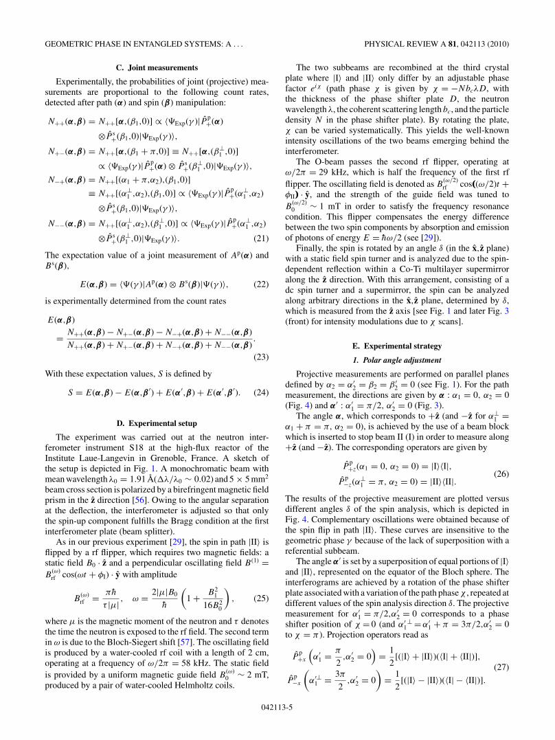
FIG. 3. (Color online) Typical interference patterns of the O-beam (α′1 = π/2) for δ = 0, π/8, π/4, π/2, 3π/4, being the direction of
the spin analysis, and geometric phase (left) γ = 0 and (right) γ = π/6. Intensities at the path phase χ = 0 and χ = π are extracted fromleast square fits of the oscillations. (rear) The resulting curves represent the projections to the ±x direction of the path subspace, denoted asP
p+x : (α′
1 = π/2, α′2 = 0) and P
p−x : (α′⊥
1 = 3π/2, α′2 = 0). The shift of the oscillations (see, e.g., δ = π/2) because of the geometric phase
γ yields a lower contrast of the curves Pp+x and P
p−x .
The interferogram obtained for γ = 0 and δ = π/2 (Fig. 3)is utilized to determine the zero point of the path phase χ ,which defines the +x direction (α′
1 = π/2, α′2 = 0) for the
path measurement.In order to obtain phase-shifter scans of higher accuracy,
scans over two periods were recorded (see Fig. 3), and thevalues for χ = 0 and π are extracted from the data by leastsquare fits. These extracted points, marking the ±x directionof the path measurement, are plotted versus different angles ofδ, as shown in Fig. 3 (rear).
All phase-shifter scans were repeated for different angles δ
for the spin analysis from δ = 0 to δ = π in steps of π/8, andfor several geometric phases γ (steps of π/6, and beginningfrom γ = π , steps of π/4), as depicted in Fig. 3 (rear) forfive selected settings of δ (δ = 0,π/8,π/4,π/2,3π/4) and twogeometric phases (γ = 0,π/6).
2. Azimuthal angle adjustment
Here the Bell angles (polar angles) remain fixed at the usualvalues and are set at δ for the projective spin measurement andby the beam block (and fixed phase shifter positions) for the
Path I (α = 0): α α = π= π)::
1
0.5
−π 0 π
Path IIPath II ((1 11
δ (rad)
P+zp>
PP-z-zpp>>
No
rmal
ized
I nte
nsi
ty (a
rb. u
nit
s)
−−−
0
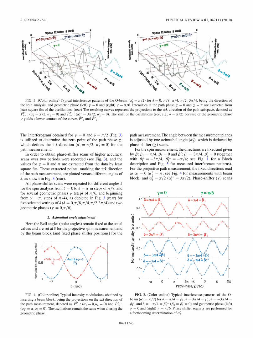
FIG. 4. (Color online) Typical intensity modulations obtained byinserting a beam block, being the projections on the ±z direction ofthe path measurement, denoted as P
p+z : (α1 = 0,α2 = 0) and P
p−z :
(α⊥1 = π,α2 = 0). The oscillations remain the same when altering the
geometric phase.
path measurement. The angle between the measurement planesis adjusted by one azimuthal angle (α′
2), which is deduced byphase-shifter (χ ) scans.
For the spin measurement, the directions are fixed and givenby β: β1 = π/4, β2 = 0 and β ′: β ′
1 = 3π/4, β ′2 = 0 (together
with β⊥1 = −3π/4, β ′⊥
1 = −π/4; see Fig. 1 for a Blochdescription and Fig. 5 for measured interference patterns).For the projective path measurement, the fixed directions readas α1 = 0 (α⊥
1 = π ; see Fig. 4 for measurements with beamblock) and α′
1 = π/2 (α′⊥1 = 3π/2). Phase-shifter (χ ) scans
0
Path Phase, Path Phase, χ χ (rad)(rad)
γ = π/6γ = π/6γ = 0γ = 0
0.5
1
0.5
1
0.5
1
0.5
1
No
rmal
ized
Inte
nsi
ty (a
rb. u
nit
s )
No
rmal
ized
Inte
nsi
ty (a
rb. u
nit
s )
δ = π/4 =δ = π/4 = β β 1
δ = 3π/4 = δ = 3π/4 = β β 1
−
δ = − π/4 = δ = − π/4 = β β 1
−
−−
δ = − 3π/4 = δ = − 3π/4 = β β 1−−
δ = π/4 =δ = π/4 = β β 1
δ = 3π/4 = δ = 3π/4 = β β 1
−
δ = − π/4 = δ = − π/4 = β β 1
−
−−
δ = − 3π/4 = δ = − 3π/4 = β β 1−−
FIG. 5. (Color online) Typical interference patterns of the O-beam (α′
1 = π/2) for δ = π/4 = β1, δ = 3π/4 = β ′1, δ = −3π/4 =
β⊥1 , and δ = −π/4 = β ′
1⊥ (β2 = β ′
2 = 0) and geometric phase (left)γ = 0 and (right) γ = π/6. Phase shifter scans χ are performed fora forthcoming determination of α′
2.
042113-6
GEOMETRIC PHASE IN ENTANGLED SYSTEMS: A . . . PHYSICAL REVIEW A 81, 042113 (2010)
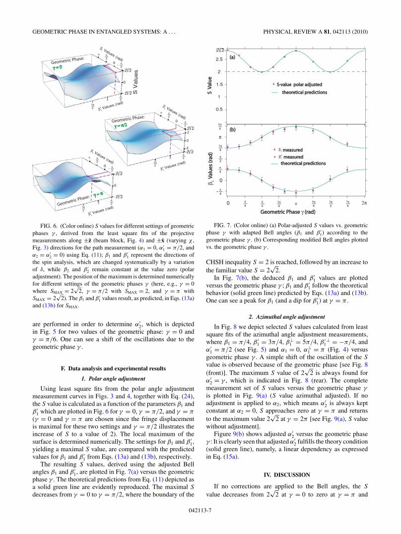
FIG. 6. (Color online) S values for different settings of geometricphases γ , derived from the least square fits of the projectivemeasurements along ±z (beam block, Fig. 4) and ±x (varying χ ,Fig. 3) directions for the path measurement (α1 = 0, α′
1 = π/2, andα2 = α′
2 = 0) using Eq. (11); β1 and β ′1 represent the directions of
the spin analysis, which are changed systematically by a variationof δ, while β2 and β ′
2 remain constant at the value zero (polaradjustment). The position of the maximum is determined numericallyfor different settings of the geometric phases γ (here, e.g., γ = 0where SMAX = 2
√2, γ = π/2 with SMAX = 2, and γ = π with
SMAX = 2√
2). The β1 and β ′1 values result, as predicted, in Eqs. (13a)
and (13b) for SMAX.
are performed in order to determine α′2, which is depicted
in Fig. 5 for two values of the geometric phase: γ = 0 andγ = π/6. One can see a shift of the oscillations due to thegeometric phase γ .
F. Data analysis and experimental results
1. Polar angle adjustment
Using least square fits from the polar angle adjustmentmeasurement curves in Figs. 3 and 4, together with Eq. (24),the S value is calculated as a function of the parameters β1 andβ ′
1 which are plotted in Fig. 6 for γ = 0, γ = π/2, and γ = π
(γ = 0 and γ = π are chosen since the fringe displacementis maximal for these two settings and γ = π/2 illustrates theincrease of S to a value of 2). The local maximum of thesurface is determined numerically. The settings for β1 and β ′
1,yielding a maximal S value, are compared with the predictedvalues for β1 and β ′
1 from Eqs. (13a) and (13b), respectively.The resulting S values, derived using the adjusted Bell
angles β1 and β ′1, are plotted in Fig. 7(a) versus the geometric
phase γ . The theoretical predictions from Eq. (11) depicted asa solid green line are evidently reproduced. The maximal S
decreases from γ = 0 to γ = π/2, where the boundary of the
Valu
es (r
ad)
Valu
es (r
ad)
Geometric Phase Geometric Phase γ (rad) (rad)
3π-4
π-4
π-2 π0 5π-
4 3π-2
7π-4
-
0
π-4
π-2
3π-4
π
5π-4
π-4
S V
alu
eS
Val
ue
S-value polar adjustedS-value polar adjusted
theoretical predictions theoretical predictions
2.5
measuredmeasured
measuredmeasured theoretical predictions theoretical predictions
-
(a)(a)
(b)(b)
1.5
0.5
2
1
2π
2 2
FIG. 7. (Color online) (a) Polar-adjusted S values vs. geometricphase γ with adapted Bell angles (β1 and β ′
1) according to thegeometric phase γ . (b) Corresponding modified Bell angles plottedvs. the geometric phase γ .
CHSH inequality S = 2 is reached, followed by an increase tothe familiar value S = 2
√2.
In Fig. 7(b), the deduced β1 and β ′1 values are plotted
versus the geometric phase γ ; β1 and β ′1 follow the theoretical
behavior (solid green line) predicted by Eqs. (13a) and (13b).One can see a peak for β1 (and a dip for β ′
1) at γ = π .
2. Azimuthal angle adjustment
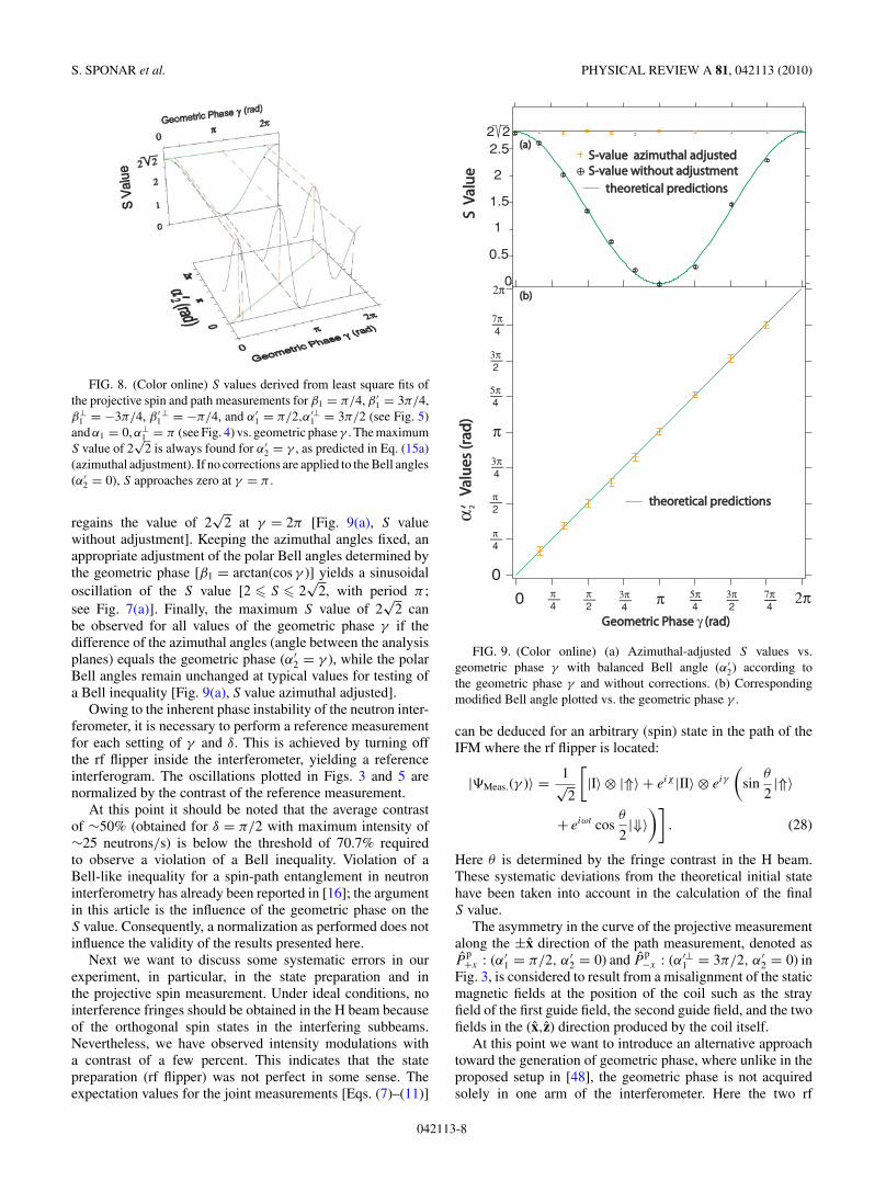
In Fig. 8 we depict selected S values calculated from leastsquare fits of the azimuthal angle adjustment measurements,where β1 = π/4, β ′
1 = 3π/4, β⊥1 = 5π/4, β ′
1⊥ = −π/4, and
α′1 = π/2 (see Fig. 5) and α1 = 0, α⊥
1 = π (Fig. 4) versusgeometric phase γ . A simple shift of the oscillation of the S
value is observed because of the geometric phase [see Fig. 8(front)]. The maximum S value of 2
√2 is always found for
α′2 = γ , which is indicated in Fig. 8 (rear). The complete
measurement set of S values versus the geometric phase γ
is plotted in Fig. 9(a) (S value azimuthal adjusted). If noadjustment is applied to α2, which means α′
2 is always keptconstant at α2 = 0, S approaches zero at γ = π and returnsto the maximum value 2
√2 at γ = 2π [see Fig. 9(a), S value
without adjustment].Figure 9(b) shows adjusted α′
2 versus the geometric phaseγ : It is clearly seen that adjusted α′
2 fulfills the theory condition(solid green line), namely, a linear dependency as expressedin Eq. (15a).
IV. DISCUSSION
If no corrections are applied to the Bell angles, the S
value decreases from 2√
2 at γ = 0 to zero at γ = π and
042113-7
S. SPONAR et al. PHYSICAL REVIEW A 81, 042113 (2010)
FIG. 8. (Color online) S values derived from least square fits ofthe projective spin and path measurements for β1 = π/4, β ′
1 = 3π/4,β⊥
1 = −3π/4, β ′1⊥ = −π/4, and α′
1 = π/2,α′⊥1 = 3π/2 (see Fig. 5)
and α1 = 0, α⊥1 = π (see Fig. 4) vs. geometric phase γ . The maximum
S value of 2√
2 is always found for α′2 = γ , as predicted in Eq. (15a)
(azimuthal adjustment). If no corrections are applied to the Bell angles(α′
2 = 0), S approaches zero at γ = π .
regains the value of 2√
2 at γ = 2π [Fig. 9(a), S valuewithout adjustment]. Keeping the azimuthal angles fixed, anappropriate adjustment of the polar Bell angles determined bythe geometric phase [β1 = arctan(cos γ )] yields a sinusoidaloscillation of the S value [2 � S � 2
√2, with period π ;
see Fig. 7(a)]. Finally, the maximum S value of 2√
2 canbe observed for all values of the geometric phase γ if thedifference of the azimuthal angles (angle between the analysisplanes) equals the geometric phase (α′
2 = γ ), while the polarBell angles remain unchanged at typical values for testing ofa Bell inequality [Fig. 9(a), S value azimuthal adjusted].
Owing to the inherent phase instability of the neutron inter-ferometer, it is necessary to perform a reference measurementfor each setting of γ and δ. This is achieved by turning offthe rf flipper inside the interferometer, yielding a referenceinterferogram. The oscillations plotted in Figs. 3 and 5 arenormalized by the contrast of the reference measurement.
At this point it should be noted that the average contrastof ∼50% (obtained for δ = π/2 with maximum intensity of∼25 neutrons/s) is below the threshold of 70.7% requiredto observe a violation of a Bell inequality. Violation of aBell-like inequality for a spin-path entanglement in neutroninterferometry has already been reported in [16]; the argumentin this article is the influence of the geometric phase on theS value. Consequently, a normalization as performed does notinfluence the validity of the results presented here.
Next we want to discuss some systematic errors in ourexperiment, in particular, in the state preparation and inthe projective spin measurement. Under ideal conditions, nointerference fringes should be obtained in the H beam becauseof the orthogonal spin states in the interfering subbeams.Nevertheless, we have observed intensity modulations witha contrast of a few percent. This indicates that the statepreparation (rf flipper) was not perfect in some sense. Theexpectation values for the joint measurements [Eqs. (7)–(11)]
S V
alu
eS
Val
ue
2.5
1.5
0.5
2
1
2 2
Geometric Phase Geometric Phase γ (rad) (rad)
3π-4
π-4
π-2
π0 5π-4
3π-2
7π-4
2π
Valu
es (r
ad)
Valu
es (r
ad)
0
α 2
-
theoretical predictions theoretical predictions
S-value azimuthal adjusted S-value azimuthal adjusted S-value without adjustment S-value without adjustment
π-4
0
π-2
3π-4
π
5π-4
3π-2
7π-4
2π
(a)(a)
(b)(b)
theoretical predictions theoretical predictions
FIG. 9. (Color online) (a) Azimuthal-adjusted S values vs.geometric phase γ with balanced Bell angle (α′
2) according tothe geometric phase γ and without corrections. (b) Correspondingmodified Bell angle plotted vs. the geometric phase γ .
can be deduced for an arbitrary (spin) state in the path of theIFM where the rf flipper is located:
|�Meas.(γ )〉 = 1√2
[|I〉 ⊗ |⇑〉 + eiχ |II〉 ⊗ eiγ
(sin
θ
2|⇑〉
+ eiωt cosθ
2|⇓〉
)]. (28)
Here θ is determined by the fringe contrast in the H beam.These systematic deviations from the theoretical initial statehave been taken into account in the calculation of the finalS value.
The asymmetry in the curve of the projective measurementalong the ±x direction of the path measurement, denoted asP
p+x : (α′
1 = π/2, α′2 = 0) and P
p−x : (α′⊥
1 = 3π/2, α′2 = 0) in
Fig. 3, is considered to result from a misalignment of the staticmagnetic fields at the position of the coil such as the strayfield of the first guide field, the second guide field, and the twofields in the (x,z) direction produced by the coil itself.
At this point we want to introduce an alternative approachtoward the generation of geometric phase, where unlike in theproposed setup in [48], the geometric phase is not acquiredsolely in one arm of the interferometer. Here the two rf
042113-8
GEOMETRIC PHASE IN ENTANGLED SYSTEMS: A . . . PHYSICAL REVIEW A 81, 042113 (2010)
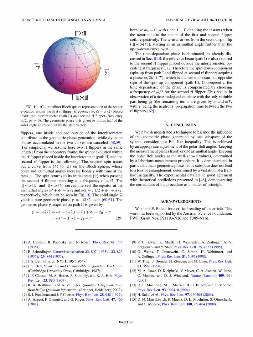
FIG. 10. (Color online) Bloch sphere representation of the spinorevolution within the first rf flipper (frequency ω, φI = π/2) placedinside the interferometer (path II) and second rf flipper (frequencyω/2, φII = 0). The geometric phase γ is given by minus half of thesolid angle �, traced out by the state vector.
flippers, one inside and one outside of the interferometer,contribute to the geometric phase generation, while dynamicphases accumulated in the two curves are canceled [58,59].(For simplicity, we assume here two rf flippers in the samelength.) From the laboratory frame, the spinor evolution withinthe rf flipper placed inside the interferometer (path II) and thesecond rf flipper is the following: The neutron spin tracesout a curve from |⇑〉 to |⇓〉 on the Bloch sphere, whosepolar and azimuthal angles increase linearly with time at therates ω. The spin returns to its initial state |⇑〉 when passingthe second rf flipper operating at a frequency of ω/2. The|⇑〉-to-|⇓〉 and |⇓〉-to-|⇑〉 curves intersect the equator at theazimuthal angles ωt + φI − π/2 and ω(t + T )/2 + φII + π/2,respectively, which can be seen in Fig. 10. The solid angle �
yields a pure geometric phase γ = −�/2, as in [60,61]. Thegeometric phase γ acquired on path II is given by
γ = −�/2 = ωt − ω/2(t + T ) + φI − φII − π
= ω(t − T )/2 + φI − π (29)
because φII = 0, with t and t + T denoting the instants whenthe neutron is at the center of the first and second flippercoil, respectively. The term π arises from the second spin flip(|⇓〉-to-|⇑〉), starting at an azimuthal angle further than theup-to-down curve by π .
The time-dependent phase is eliminated, as already dis-cussed in Sec. III B; the reference beam (path I) is also exposedto the second rf flipper placed outside the interferometer, op-erating at frequency ω/2. Therefore the spin-down component(spin-up from path I and flipped at second rf flipper) acquiresa phase ω/2(t + T ), which is the same amount but oppositesign of the spin-up component (path II). Consequently, thetime dependence of the phase is compensated by choosinga frequency of ω/2 for the second rf flipper. This results inobservation of a time-independent phase with the only variablepart being φI (the remaining terms are given by π and ωT ,with T being the neutrons’ propagation time between the tworf flippers [62]).
V. CONCLUSION
We have demonstrated a technique to balance the influenceof the geometric phase generated by one subspace of thesystem, considering a Bell-like inequality. This is achievedby an appropriate adjustment of the polar Bell angles (keepingthe measurement planes fixed) or one azimuthal angle (keepingthe polar Bell angles at the well-known values), determinedby a laborious measurement procedure. It is demonstrated, inparticular, that a geometric phase in one subspace does not leadto a loss of entanglement, determined by a violation of a Bell-like inequality. The experimental data are in good agrementwith theoretical predictions presented in [48], demonstratingthe correctness of the procedure as a matter of principle.
ACKNOWLEDGMENTS
We thank E. Balcar for a critical reading of the article. Thiswork has been supported by the Austrian Science Foundation,FWF (Grant Nos. P21193-N20 and T389-N16).
[1] A. Einstein, B. Podolsky, and N. Rosen, Phys. Rev. 47, 777(1935).
[2] E. Schrodinger, Naturwissenschaften 23, 807 (1935); 23, 823(1935); 23, 844 (1935).
[3] J. S. Bell, Physics (NY) 1, 195 (1964).[4] J. S. Bell, Speakable and Unspeakable in Quantum Mechanics
(Cambridge University Press, Cambridge, 1987).[5] J. F. Clauser, M. A. Horne, A. Shimony, and R. A. Holt, Phys.
Rev. Lett. 23, 880 (1969).[6] R. A. Bertlmann and A. Zeilinger, Quantum [Un]speakables,
from Bell to Quantum Information (Springer, Heidelberg, 2002).[7] S. J. Freedman and J. F. Clauser, Phys. Rev. Lett. 28, 938 (1972).[8] A. Aspect, P. Grangier, and G. Roger, Phys. Rev. Lett. 47, 460
(1981).
[9] P. G. Kwiat, K. Mattle, H. Weinfurter, A. Zeilinger, A. V.Sergienko, and Y. Shih, Phys. Rev. Lett. 75, 4337 (1995).
[10] G. Weihs, T. Jennewein, C. Simon, H. Weinfurter, andA. Zeilinger, Phys. Rev. Lett. 81, 5039 (1998).
[11] W. Tittel, J. Brendel, H. Zbinden, and N. Gisin, Phys. Rev. Lett.81, 3563 (1998).
[12] M. A. Rowe, D. Kielpinski, V. Meyer, C. A. Sackett, W. Itano,C. Monroe, and D. J. Wineland, Nature (London) 409, 791(2001).
[13] D. L. Moehring, M. J. Madsen, B. B. Blinov, and C. Monroe,Phys. Rev. Lett. 93, 090410 (2004).
[14] H. Sakai et al., Phys. Rev. Lett. 97, 150405 (2006).[15] D. N. Matsukevich, P. Maunz, D. L. Moehring, S. Olmschenk,
and C. Monroe, Phys. Rev. Lett. 100, 150404 (2008).
042113-9

S. SPONAR et al. PHYSICAL REVIEW A 81, 042113 (2010)
[16] Y. Hasegawa, R. Loidl, G. Badurek, M. Baron, and H. Rauch,Nature (London) 425, 45 (2003).
[17] J. S. Bell, Rev. Mod. Phys. 38, 447 (1966).[18] N. D. Mermin, Rev. Mod. Phys. 65, 803 (1993).[19] C. Simon, M. Zukowski, H. Weinfurter, and A. Zeilinger, Phys.
Rev. Lett. 85, 1783 (2000).[20] S. Kochen and E. P. Specker, J. Math. Mech. 17, 59 (1967).[21] A. Cabello, Phys. Rev. Lett. 101, 210401 (2008).[22] A. Cabello, S. Filipp, H. Rauch, and Y. Hasegawa, Phys. Rev.
Lett. 100, 130404 (2008).[23] G. Kirchmair, F. Zahringer, R. Gerritsma, M. Kleinmann,
O. Guhne, A. Cabello, R. Blatt, and C. F. Roos, Nature (London)460, 494 (2009).
[24] Y. Hasegawa, R. Loidl, G. Badurek, M. Baron, and H. Rauch,Phys. Rev. Lett. 97, 230401 (2006).
[25] H. Bartosik, J. Klepp, C. Schmitzer, S. Sponar, A. Cabello,H. Rauch, and Y. Hasegawa, Phys. Rev. Lett. 103, 040403(2009).
[26] H. Rauch, W. Treimer, and U. Bonse, Phys. Lett. A 47, 369(1974).
[27] H. Rauch and S. A. Werner, Neutron Interferometry (ClarendonPress, Oxford, 2000).
[28] Y. Hasegawa, R. Loidl, G. Badurek, S. Filipp, J. Klepp, andH. Rauch, Phys. Rev. A 76, 052108 (2007).
[29] S. Sponar, J. Klepp, R. Loidl, S. Filipp, G. Badurek,Y. Hasegawa, and H. Rauch, Phys. Rev. A 78, 061604(R) (2008).
[30] M. V. Berry, Proc. R. Soc. London A 392, 45 (1984).[31] A. Tomita and R. Y. Chiao, Phys. Rev. Lett. 57, 937 (1986).[32] T. Bitter and D. Dubbers, Phys. Rev. Lett. 59, 251 (1987).[33] Y. Aharonov and J. Anandan, Phys. Rev. Lett. 58, 1593 (1987).[34] J. Samuel and R. Bhandari, Phys. Rev. Lett. 60, 2339 (1988).[35] S. Pancharatnam, Proc. Indian Adac. Sci. A 44, 247 (1956).[36] N. Manini and F. Pistolesi, Phys. Rev. Lett. 85, 3067 (2000).[37] Y. Hasegawa, R. Loidl, M. Baron, G. Badurek, and H. Rauch,
Phys. Rev. Lett. 87, 070401 (2001).[38] Y. Hasegawa, R. Loidl, G. Badurek, M. Baron, N. Manini,
F. Pistolesi, and H. Rauch, Phys. Rev. A 65, 052111 (2002).[39] E. Sjoqvist, A. K. Pati, A. Ekert, J. S. Anandan, M. Ericsson,
D. K. L. Oi, and V. Vedral, Phys. Rev. Lett. 85, 2845 (2000).[40] S. Filipp and E. Sjoqvist, Phys. Rev. A 68, 042112 (2003).[41] S. Filipp and E. Sjoqvist, Phys. Rev. Lett. 90, 050403 (2003).
[42] J. Klepp, S. Sponar, Y. Hasegawa, E. Jericha, and G. Badurek,Phys. Lett. A 342, 48 (2005).
[43] J. Klepp, S. Sponar, S. Filipp, M. Lettner, G. Badurek, andY. Hasegawa, Phys. Rev. Lett. 101, 150404 (2008).
[44] M. A. Nielsen and I. Chuang, Quantum Computation andQuantum Information (Cambridge University Press, Cambridge,2000).
[45] P. J. Leek, J. M. Fink, A. Blais, R. Bianchetti, M. Goppl,J. M. Gambetta, D. I. Schuster, L. Frunzio, R. J. Schoelkopf, andA. Wallraff, Science 318, 1889 (2007).
[46] S. Filipp, J. Klepp, Y. Hasegawa, C. Plonka-Spehr, U. Schmidt,P. Geltenbort, and H. Rauch, Phys. Rev. Lett. 102, 030404(2009).
[47] E. Sjoqvist, Phys. Rev. A 62, 022109 (2000).[48] R. A. Bertlmann, K. Durstberger, Y. Hasegawa, and B. C.
Hiesmayr, Phys. Rev. A 69, 032112 (2004).[49] D. M. Tong, L. C. Kwek, and C. H. Oh, J. Phys. A 36, 1149
(2003).[50] R. Das, S. K. Kumar, and A. Kumar, J. Magn. Reson. 177, 318
(2005).[51] S. Basu, S. Bandyopadhyay, G. Kar, and D. Home, Phys. Lett.
A 279, 281 (2001).[52] R. Gahler and R. Golub, Phys. Lett. A 123, 43 (1987).[53] R. Golub, R. Gahler, and T. Keller, Am. J. Phys. 62, 779
(1994).[54] S. V. Grigoriev, W. H. Kraan, and M. T. Rekveldt, Phys. Rev. A
69, 043615 (2004).[55] D. Suter, K. T. Mueller, and A. Pines, Phys. Rev. Lett. 60, 1218
(1988).[56] G. Badurek, R. J. Buchelt, G. Kroupa, M. Baron, and M. Villa,
Physica B 283, 389 (2000).[57] F. Bloch and A. Siegert, Phys. Rev. 57, 522 (1940).[58] S.-L. Zhu and Z. D. Wang, Phys. Rev. A 67, 022319 (2003).[59] Y. Ota, Y. Goto, Y. Kondo, and M. Nakahara, Phys. Rev. A 80,
052311 (2009).[60] A. G. Wagh, G. Badurek, V. C. Rakhecha, R. J. Buchelt, and
A. Schricker, Phys. Lett. A 268, 209 (2000).[61] B. E. Allman, H. Kaiser, S. A. Werner, A. G. Wagh, V. C.
Rakhecha, and J. Summhammer, Phys. Rev. A 56, 4420 (1997).[62] S. Sponar, J. Klepp, G. Badurek, and Y. Hasegawa, Phys. Lett.
A 372, 3153 (2008).
042113-10