geometric numerical integration applied to the elastic pendulum at higher-order resonance

Journal of Computational and Applied Mathematics 154 (2003) 229–242www.elsevier.com/locate/cam

Geometric numerical integration applied to the elasticpendulum at higher-order resonance

J.M. Tuwankottaa ;∗;1, G.R.W. Quispelb

aMathematisch Instituut, Universiteit Utrecht, P.O. Box 80.010, 3508 TA Utrecht, The NetherlandsbSchool of Mathematical and Statistical Sciences, La Trobe University, Bundoora, Vic. 3083, Australia

Received 1 February 2002; received in revised form 15 September 2002

Abstract

In this paper, we study the performance of a symplectic numerical integrator based on the splitting method.This method is applied to a subtle problem i.e. higher-order resonance of the elastic pendulum. In order tonumerically study the phase space of the elastic pendulum at higher order resonance, a numerical integratorwhich preserves qualitative features after long integration times is needed. We show by means of an examplethat our symplectic method o4ers a relatively cheap and accurate numerical integrator.c© 2003 Elsevier Science B.V. All rights reserved.

MSC: 34C15; 37M15; 65P10; 70H08

Keywords: Hamiltonian mechanics; Higher-order resonance; Elastic pendulum; Symplectic numerical integration;Geometric integration

1. Introduction

Higher-order resonances are known to have a long time-scale behaviour. From an asymptotic pointof view, a =rst-order approximation (such as =rst-order averaging) would not be able to clarify theinteresting dynamics in such a system. Numerically, this means that the integration times neededto capture such behaviour are signi=cantly increased. In this paper we present a reasonably cheapmethod to achieve a qualitatively good result even after long integration times.

Geometric numerical integration methods for (ordinary) di4erential equations ([2,10,13]) haveemerged in the last decade as alternatives to traditional methods (e.g., Runge–Kutta methods).

∗ Corresponding author.E-mail address: [email protected] (J.M. Tuwankotta).

1 On leave from Jurusan Matematika, FMIPA, Institut Teknologi Bandung, Ganesha no. 10, Bandung, Indonesia.

0377-0427/03/$ - see front matter c© 2003 Elsevier Science B.V. All rights reserved.PII: S0377-0427(02)00825-7

mailto:[email protected]

230 J.M. Tuwankotta, G.R.W. Quispel / Journal of Computational and Applied Mathematics 154 (2003) 229–242

Geometric methods are designed to preserve certain properties of a given ODE exactly (i.e., with-out truncation error). The use of geometric methods is particularly important for long integrationtimes. Examples of geometric integration methods include symplectic integrators, volume-preservingintegrators, symmetry-preserving integrators, integrators that preserve =rst integrals (e.g., energy),Lie-group integrators, etc. A survey is given in [10].

It is well known that resonances play an important role in determining the dynamics of a givensystem. In practice, higher-order resonances occur more often than lower order ones, but their analysisis more complicated. In [12], Sanders was the =rst to give an upper bound on the size of the resonancedomain (the region where interesting dynamics takes place) in two degrees of freedom Hamiltoniansystems. Numerical studies by van den Broek [16], however, provided evidence that the resonancedomain is actually much smaller. In [15], Tuwankotta and Verhulst derived improved estimates forthe size of the resonance domain, and provided numerical evidence that for the 4:1 and the 6:1resonances of the elastic pendulum, their estimates are sharp. The numerical method they used intheir analysis, 2 however, was not powerful enough to be applied to higher-order resonances. In thispaper we construct a symplectic integration method, and use it to show numerically that the estimatesof the size of the resonance domain in [15] are also sharp for the 4:3 and the 3:1 resonances.

Another subtle problem regarding to this resonance manifold is the bifurcation of this manifold asthe energy increases. To study this problem numerically one would need a numerical method whichis reasonably cheap and accurate after a long integration times.

In this paper we will use the elastic pendulum as an example. The elastic pendulum is a wellknown (classical) mechanical problem which has been studied by many authors. One of the reasonsis that the elastic pendulum can serve as a model for many problems in di4erent =elds. See thereferences in [4,15]. In itself, the elastic pendulum is a very rich dynamical system. For di4erentresonances, it can serve as an example of a chaotic system, an auto-parametric excitation system([17]), or even a linearizable system. The system also has (discrete) symmetries which turn out tocause degeneracy in the normal form.

We will =rst give a brief introduction to the splitting method which is the main ingredient forthe symplectic integrator in this paper. We will then collect the analytical results on the elasticpendulum that have been found by various authors. Mostly, in this paper we will be concerned withthe higher-order resonances in the system. All of this will be done in the next two sections of thepaper. In the fourth section we will compare our symplectic integrator with the standard 4th orderRunge–Kutta method and also with an order 7–8 Runge–Kutta method. We end the fourth sectionby calculating the size of the resonance domain of the elastic pendulum at higher-order resonance.

2. Symplectic integration

Consider a symplectic space �=R2n, n∈N where each element � in � has coordinate (q; p) andthe symplectic form is dq ∧ dp. For any two functions F;G ∈C∞(�) de=ne

{F;G} =n∑1

(9F9qj

9G9pj

− 9G9qj

9F9pj

)∈C∞(�);

2 A Runge–Kutta method of order 7–8.

J.M. Tuwankotta, G.R.W. Quispel / Journal of Computational and Applied Mathematics 154 (2003) 229–242 231

which is called the Poisson bracket of F and G. Every function H ∈C∞(�) generates a (Hamilto-nian) vector =eld de=ned by {qi; H}, {pi; H}; i = 1; : : : ; n. The dynamics of H is then governed bythe equations of motion of the form

qi = {qi; H}pi = {pi; H}; i = 1; : : : ; n:

Let X and Y be two Hamiltonian vector =elds, de=ned in �, associated with Hamiltonians HX

and HY in C∞(�), respectively. Consider another vector =eld [X; Y ] which is just the commutatorof the vector =elds X and Y . Then [X; Y ] is also a Hamiltonian vector =eld with HamiltonianH[X;Y ] = {HX ;HY}. See, for example [1,7,11] for details.

We can write the Low of the Hamiltonian vector =elds X as

’X ;t = exp(tX ) ≡ I + tX +12!

(tX )2 +13!

(tX )3 + · · ·(and so does the Low of Y ). By the Baker–Campbell–Hausdor4 formula, there exists a (formal)Hamiltonian vector =eld Z such that

Z = (X + Y ) +t2

[X; Y ] +t2

12([X; X; Y ] + [Y; Y; X ]) + O(t3) (1)

and exp(tZ) = exp(tX ) exp(tY ), where [X; X; Y ] = [X; [X; Y ]], and so on. Moreover, Yoshida (in [19])shows that exp(tX ) exp(tY ) exp(tX ) = exp(tZ), where

Z = (2X + Y ) +t2

6([Y; Y; X ] − [X; X; Y ]) + O(t4): (2)

We note that in terms of the Low, the multiplication of the exponentials above means compositionof the corresponding Low, i.e., ’Y ;t ◦ ’X ;t .

Let �∈R be a small positive number and consider a Hamiltonian system with Hamiltonian H (�)=HX (�) +HY (�), where � ∈�, and �=X +Y . Using (1) we have that ’Y ;� ◦’X ;� is (approximately)the Low of a Hamiltonian system

� = (X + Y ) +�2

[X; Y ] +�2

12([X; X; Y ] + [Y; Y; X ]) + O(�3);

with Hamiltonian

H� = HX + HY +�2{HX ;HY} +

�2

12({HX ;HX ; HY} + {HY ; HY ; HX }) + O(�3):

Note that {H;K; F} = {H; {K; F}}. This mean that H − H� = O(�) or, in other words

’Y ;� ◦ ’X ;� = ’X+Y (�) + O(�2): (3)

As before and using (2), we conclude that

’X ;�=2 ◦ ’Y ;� ◦ ’X ;�=2 = ’X+Y (�) + O(�3): (4)

Suppose that X ;� and Y ;� are numerical integrators of system � = X and � = Y (respectively).We can use symmetric composition (see [8]) to improve the accuracy of X+Y ;�. If Y ;� and X ;�

are symplectic, then the composition forms a symplectic numerical integrator for X + Y . See [13]for more discussion; also [10] for references. If we can split H into two (or more) parts which


Poisson commute with each other (i.e., the Poisson brackets between each pair vanish), then wehave H = H�. This implies that in this case the accuracy of the approximation depends only on theaccuracy of the integrators for X and Y . An example of this case is when we are integrating theBirkho4 normal form of a Hamiltonian system.

3. The elastic pendulum

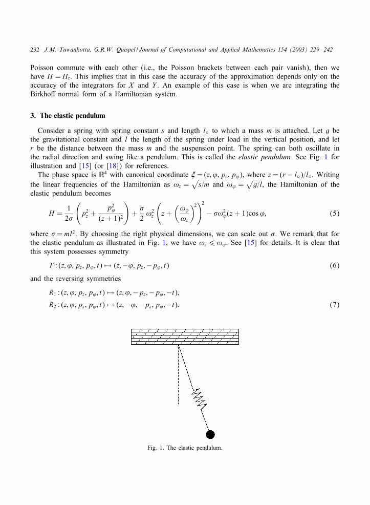
Consider a spring with spring constant s and length l◦ to which a mass m is attached. Let g bethe gravitational constant and l the length of the spring under load in the vertical position, and letr be the distance between the mass m and the suspension point. The spring can both oscillate inthe radial direction and swing like a pendulum. This is called the elastic pendulum. See Fig. 1 forillustration and [15] (or [18]) for references.

The phase space is R4 with canonical coordinate � = (z; ’; pz; p’), where z = (r− l◦)=l◦. Writingthe linear frequencies of the Hamiltonian as !z =

√s=m and !’ =

√g=l, the Hamiltonian of the

elastic pendulum becomes

H =1

2�

(p2

z +p2

’

(z + 1)2

)+

�2!2

z

(z +

(!’

!z

)2)2

− �!2’(z + 1)cos’; (5)

where � = ml2. By choosing the right physical dimensions, we can scale out �. We remark that forthe elastic pendulum as illustrated in Fig. 1, we have !z6!’. See [15] for details. It is clear thatthis system possesses symmetry

T : (z; ’; pz; p’; t) → (z;−’;pz;−p’; t) (6)

and the reversing symmetries

R1 : (z; ’; pz; p’; t) → (z; ’;−pz;−p’;−t);

R2 : (z; ’; pz; p’; t) → (z;−’;−pz; p’;−t): (7)

Fig. 1. The elastic pendulum.


If there exist two integers k1 and k2 such that k1!z + k2!’ = 0, then we say !z and !’ are inresonance. Assuming (|k1|; |k2|) = 1, we can divide the resonances in two types, e.g., lower-orderresonance if |k1| + |k2|¡ 5 and higher-order resonance if |k1| + |k2|¿ 5. In the theory of normalforms, the type of normal form of the Hamiltonian is highly dependent on the type of resonance inthe system. See [1].

In general, the elastic pendulum has at least one =xed point which is the origin of phase space.This =xed point is elliptic. For some of the resonances, there is also another =xed point which isof the saddle type, i.e. (z; ’; pz; p’) = (−2(!’=!z)2; "; 0; 0). From the de=nition of z, it is clear thatthe latter =xed point only exists for !z=!’ ¿

√2. The elastic pendulum also has a special periodic

solution in which ’ = p’ = 0 (the normal mode). This normal mode is an exact solution of thesystem derived from (5). We note that there is no nontrivial solution of the form (0; ’(t); 0; p’(t)).

Now we turn our attention to the neighborhood of the origin. We refer to [15] for the completederivation of the following Taylor expansion of the Hamiltonian (we have dropped the bar)

H = H2 + $H3 + $2H4 + $3H5 + · · · ; (8)

with

H2 = 12 !z(z2 + p2

z ) + 12 !’(’2 + p2

’);

H3 =!’√!z

( 12z’

2 − zp2’);

H4 =(

32

!’

!zz2p2

’ − 124

’4

);

H5 = − 1√!z

(124

z’4 + 2!’

!zz3p2

’

);

...

In [17] the 2:1-resonance of the elastic pendulum has been studied intensively. At this speci=cresonance, the system exhibits an interesting phenomenon called auto-parametric excitation, e.g.,if we start at any initial condition arbitrarily close to the normal mode, then we will see energyinterchanging between the oscillating and swinging motion. In [3], the author shows that the normalmode solution (which is the vertical oscillation) is unstable and therefore, gives an explanation ofthe auto-parametric behavior.

Next we consider two limiting cases of the resonances, i.e., when !z=!’ → ∞ and !z=!’ → 1.The =rst limiting case can be interpreted as a case with a very large spring constant so that thevertical oscillation can be neglected. The spring pendulum then becomes an ordinary pendulum; thusthe system is integrable. The other limiting case is interpreted as the case where l◦=0 (or very weakspring). 3 Using the transformation r=l(z+1); x=r cos’ and y=r sin ’, we transform Hamiltonian(5) to the Hamiltonian of the harmonic oscillator. Thus this case is also integrable. Furthermore, inthis case all solutions are periodic with the same period which is known as isochronism. This means

3 This case is unrealistic for the model illustrated in Fig. 1. A more realistic mechanical model with the same Hamiltonian(5) can be constructed by only allowing some part of the spring to swing.


that we can remove the dependence of the period of oscillation of the mathematical pendulum on theamplitude, using this speci=c spring. We note that this isochronism is not derived from the normalform (as in [18]) but exact.

All other resonances are higher order resonances. In two degrees of freedom (which is the casewe consider), for =xed small energy the phase space of the system near the origin looks like thephase space of decoupled harmonic oscillator. A consequence of this fact is that in the neighborhoodof the origin, there is no interaction between the two degrees of freedom. The normal mode (if itexists), then becomes elliptic (thus stable).

Another possible feature of this type of resonance is the existence of a resonance manifold con-taining periodic solutions (see [5] paragraph 4.8). We remark that the existence of this resonancemanifold does not depend on whether the system is integrable or not. In the resonance domain (i.e.,the neighborhood of the resonant manifold), interesting dynamics (in the sense of energy interchang-ing between the two degrees of freedom) takes place (see [12]). Both the size of the domain wherethe dynamics takes place and the time-scale of interaction are characterized by $ and the order ofthe resonance, i.e., the estimate of the size of the domain is

d$ = O($(m+n−4)=2) (9)

and the time-scale of interactions is O($−(m+n)=2) for !z :!’ = m : n with (m; n) = 1: 4 We note thatfor some of the higher-order resonances where !z=!’ ≈ 1 the resonance manifold fails to exist. See[15] for details.

4. Numerical studies on the elastic pendulum

One of the aims of this study is to construct a numerical PoincarQe map (P) for the elasticpendulum in higher-order resonance. As is explained in the previous section, interesting dynamicsof the higher-order resonances takes place in a rather small part of phase space. Moreover, theinteraction time-scale is also rather long. For these two reasons, we need a numerical method whichpreserves qualitative behavior after a long time of integration. Obviously by decreasing the timestep of any standard integrator (e.g. Runge–Kutta method), we would get a better result. As aconsequence, however, the actual computation time would become prohibitively long. Under theseconstraints, we would like to propose by means of an example that symplectic integrators o4erreliable and reasonably cheap methods to obtain qualitatively good phase portraits.

We have selected four of the most prominent higher-order resonances in the elastic pendulum.For each of the chosen resonances, we derive its corresponding equations of motion from (8). Thisis done because the dependence on the small parameter $ is more visible there than in (5). Alsofrom the asymptotic analysis point of view, we know that (8) truncated to a suRcient degree hasenough ingredients of the dynamics of (5).

The map P is constructed as follows. We choose the initial values �◦ in such a way that they alllie in the approximate energy manifold H2 = E◦ ∈R and in the section ) = {� = (z; ’; pz; p’) | z =0; pz ¿ 0}. We follow the numerically constructed trajectory corresponding to �◦ and take the in-

4 Due to a particular symmetry, some of the lower order resonances become higher-order resonances ([15]). In thosecases, (m; n) = 1 need not hold.


tersection of the trajectory with section ). The intersection point is de=ned as P(�◦). Starting fromP(�◦) as an initial value, we go on integrating and in the same way we =nd P2(�◦), and so on.

The best way of measuring the performance of a numerical integrator is by comparing with anexact solution. Due to the presence of the normal mode solution (as an exact solution), we cancheck the performance of the numerical integrator in this way (we will do this in Section 4.2).Nevertheless, we should remark that none of the nonlinear terms play a part in this normal modesolution. Recall that the normal mode is found in the invariant manifold {(z; ’; pz; p’ |’ = p’ = 0}and in this manifold the equations of motion of (8) are linear.

Another way of measuring the performance of an integrator is to compare it with other methods.One of the best known methods for time integration are the Runge–Kutta methods (see [6]). We willcompare our integrator with a higher order (7–8 order) Runge–Kutta method (RK78). The RK78is based on the method of Runge–Kutta–Felbergh ([14]). The advantage of this method is that itprovides step-size control. As is indicated by the name of the method, to choose the optimal stepsize it compares the discretizations using 7th order and 8th order Runge–Kutta methods. A nicediscussion on lower order methods of this type, can be found in [14, pp. 448–454]. The coeRcientsin this method are not uniquely determined. For RK78 that we used in this paper, the coeRcientswere calculated by C. Simo from the University of Barcelona. We will also compare the symplecticintegrator (SI) to the standard 4th order Runge–Kutta method.

We will =rst describe the splitting of the Hamiltonian which is at the core of the symplecticintegration method in this paper. By combining the Low of each part of the Hamiltonian, we constructa 4th order symplectic integrator. The symplecticity is obvious since it is the composition of exactHamiltonian Lows. Next we will show the numerical comparison between the three integrators,RK78, SI and RK4. We compare them to an exact solution. We will also show the performanceof the numerical integrators with respect to energy preservation. We note that SI are not designedto preserve energy (see [10]). Because RK78 is a higher order method (thus more accurate), wewill also compare the orbit of RK4 and SI. We will end this section with results on the size of theresonance domain calculated by the SI method.

4.1. The splitting of the Hamiltonian

Consider again the expanded Hamiltonian of the elastic pendulum (8). We split this Hamiltonianinto integrable parts: H = H 1 + H 2 + H 3, where

H 1 = $!’

2√!z

z’2 − $2 124

’4 − $3 124

√!z

z’4 + · · · ;

H 2 = −$!’√!z

zp2’ + $2 3

2!’

!zz2p2

’ − $3 2!’

!z√!z

z3p2’ + · · · ;

H 3 = 12 !z(z2 + p2

z ) + 12 !’(’2 + p2

’): (10)

Note that the equations of motion derived from each part of the Hamiltonian can be integrated ex-actly; thus we know the exact Low ’1;�; ’2;�, and ’3;� corresponding to H 1; H 2, and H 3, respectively.This splitting has the following advantages:


• It preserves the Hamiltonian structure of the system.• It preserves the symmetry (6) and reversing symmetries (7) of H .• H 1 and H 2 are of O($) compared with H (or H 3).

Note that, for each resonance we will truncate (10) up to and including the degree where the resonantterms of the lowest order occur.

We de=ne

’� = ’1;�=2 ◦ ’2;�=2 ◦ ’3;� ◦ ’2;�=2 ◦ ’1;�=2: (11)

From Section 2 we know that this is a second-order method. Next we de=ne * = 1=(2 − 3√

2) and � = ’*� ◦ ’(1−2*)� ◦ ’*� to get a fourth-order method. This is known as the generalized Yoshidamethod (see [10]). By, Symplectic Integrator (SI) we will mean this fourth-order method. Thiscomposition preserves the symplectic structure of the system, as well as the symmetry (6) and thereversing symmetries (7). This is in contrast with the Runge–Kutta methods which only preserves thesymmetry (6), but not the symplectic structure, nor the reversing symmetries (7). As a consequencethe Runge–Kutta methods do not preserve the KAM tori caused by symplecticity or reversibility.

4.2. Numerical comparison between RK4, RK78 and SI

We start by comparing the three numerical methods, i.e., RK4, RK78, and SI. We choose the4:1-resonance, which is the most prominent higher-order resonance, as a test problem. We =x thevalue of the energy (H2) to be 5 and take $= 0:05. Starting at the initial condition z(0) = 0; ’(0) =0; pz =

√5=2, and p’(0) = 0, we know that the exact solution we are approximating is given by

(√

5=2 sin(4t); 0;√

5=2 cos(4t); 0). We integrate the equations of motion up to t = 105 s and keepthe result of the last 10 s to have time series Sz(tn) and pz(tn) produced by each integrator. Then wede=ne a sequence sn = 99990 + 5n=100; n= 0; 1; : : : ; 200. Using an interpolation method, for each ofthe time series we calculate the numerical Sz(sn). In Fig. 2 we plot the error function Sz(sn) − z(sn)for each integrator.

The plots in Fig. 2 clearly indicate the superiority of RK78 compared with the other methods (dueto the higher-order method). The error generated by RK78 is of order 10−7 for an integration timeof 105 s. The minimum time step taken by RK78 is 0.0228 and the maximum is 0.0238. The errorgenerated by SI on the other hand, is of order 10−5. The CPU time of RK78 during this integrationis 667:75 s. SI completes the computation after 446:72 s while RK4 only needs 149:83 s.

We will now measure how well these integrators preserve energy. We start integrating from aninitial condition z(0) = 0; ’(0) = 1:55; p’(0) = 0 and pz(0) is determined from H 3 = 5 (in otherword we integrate on the energy manifold H = 5 + O($)). The small parameter is $ = 0:05 and weintegrate for t = 105 s.

For RK78, the integration takes 667:42 s of CPU time. For RK4 and SI we used the same timestep, that is 10−2. RK4 takes 377:35 s while SI takes 807:01 s of CPU time. It is clear that SI, forthis size of time step, is ineRcient with regard to CPU time. This is due to the fact that to constructa higher-order method we have to compose the Low several times. We plot the results of the last10 s of the integrations in Fig. 3. We note that in these 10 s, the largest time step used by RK78 is0:02421 : : : while the smallest is 0:02310 : : : . It is clear from this, that even though the CPU time


Fig. 2. Plots of the error function Sz(sn) − z(sn) against time. The upper =gure is the result of RK4, the middle =gure isRK78 and the lower =gure is of SI. The time of integration is 105 with a time step for RK4 and SI of 0.025.

Fig. 3. Plots of the energy against time. The solid line represents the results from SI. The line with ‘+’ represents theresults from RK4 and the line with ‘◦’ represents the results from RK78. On the left-hand plot, we show the results ofall three methods with the time step 0.01. The time step in the right-hand plots is 0.05. The results from RK4 are plottedseparately since the energy has decreased signi=cantly compared to the other two methods.


Fig. 4. Resonance domain for the 4:1-resonance. The plots on the left are the results from SI while the right-hand plotsare the results from RK78. The vertical axis is the p’ axis and the horizontal axis is ’. The time step is 0.05 and $=0:05.In the top =gures, we blow up a part of the pictures underneath.

of RK4 is very good, the result in the sense of conservation of energy is rather poor relative to theother methods.

We increase the time step to 0.05 and integrate the equations of motion starting at the same initialcondition and for the same time. The CPU time of SI is now 149.74 while for the RK4 it is 76.07.Again, in Fig. 3 (the right-hand plots) we plot the energy against time. A signi=cant di4erencebetween RK4 and SI then appears in the energy plots. The results of symplectic integration are stillgood compared with the higher-order method RK78. On the other hand, the results from RK4 arefar below the other two.

4.3. Computation of the size of the resonance domain

Finally, we calculate the resonance domain for some of the most prominent higher-order resonancesfor the elastic pendulum. In Fig. 4 we give an example of the resonance domain for the 4:1 resonance.We note that RK4 fails to produce the section. On the other hand, the results from SI are stillaccurate. We compare the results from SI and RK78 in Fig. 4. After 5× 103 s, one loop in the plotis completed. For that time of integration, RK78 takes 34:92 s of CPU time, while SI takes only16:35 s.


Table 1Comparison between the analytic estimate and the numerical computation ofthe size of the resonance domain of four of the most prominent higher-orderresonances of the elastic pendulum. The second column of this table indicatesthe part of the expanded Hamiltonian in which the lowest-order resonant termsare found

Resonance Resonant Analytic Numerical Errorpart log$(d$) log$(d$)

4:1 H5 1/2 0.5091568 0.016:1 H7 3/2 1.5079998 0.054:3 H7 3/2 1.4478968 0.093:1 H8 2 2.0898136 0.35

This is very useful since to calculate for smaller values of $ and higher resonance cases, theintegration time is a lot longer which makes it impractical to use RK78.

In Table 1 we list the four most prominent higher order resonances for the elastic pendulum. Thistable is adopted from [15] where the authors list six of them.

The numerical size of the domain in Table 1 is computed as follows. We =rst draw severalorbits of the PoincarQe maps P. Using a twist map argument, we can locate the resonance domain.By adjusting the initial condition manually, we then approximate the heteroclinic cycle of P. SeeFig. 4 for illustration. Using interpolation we construct the function ro(,) which represent the distanceof a point in the outer cycle to the origin and , is the angle with respect to the positive horizontalaxis. We do the same for the inner cycle and then calculate max, |ro(,) − ri(,)|. The higher theresonance is, the more diRcult to compute the size of the domain in this way.

For resonances with very high order, manually approximating the heteroclinic cycles would becomeimpractical, and one could do the following. First we have to calculate the location of the =xed pointsof the iterated PoincarQe maps numerically. Then we can construct approximations of the stable andunstable manifolds of one of the saddle points. By shooting to the next saddle point, we can makecorrections to the approximate stable and unstable manifold of the =xed point.

5. Discussion

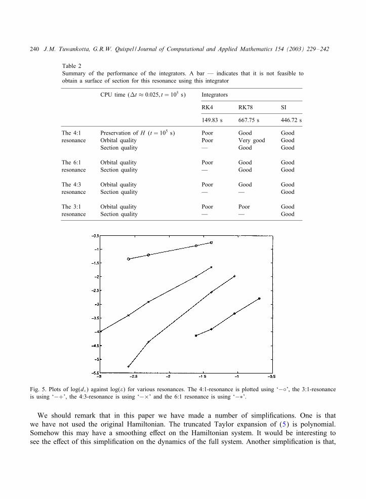
In this section we summarize the previous sections. First the performance of the integrators issummarized in Table 2 (Fig. 5).

As indicated in Table 2, for the 4:3 and the 3:1 resonances, the higher-order Runge–Kutta methodfails to produce the section. This is caused by the dissipation term, arti=cially introduced by thisnumerical method, which after a long time of integration starts to be more signi=cant. On the otherhand, we conclude that the results of our symplectic integrator are reliable. This conclusion is alsosupported by the numerical calculations of the size of the resonance domain (listed in Table 2).

In order to force the higher-order Runge–Kutta method to be able to produce the section, onecould also do the following. Keeping in mind that RK78 has automatic step size control based onthe smoothness of the vector =eld, one could manually set the maximum time step for RK78 to besmaller than 0.02310. This would make the integration times extremely long however.


Table 2Summary of the performance of the integrators. A bar — indicates that it is not feasible toobtain a surface of section for this resonance using this integrator

CPU time (Wt ≈ 0:025; t = 105 s) Integrators

RK4 RK78 SI

149:83 s 667:75 s 446:72 s

The 4:1 Preservation of H (t = 105 s) Poor Good Goodresonance Orbital quality Poor Very good Good

Section quality — Good Good

The 6:1 Orbital quality Poor Good Goodresonance Section quality — Good Good

The 4:3 Orbital quality Poor Good Goodresonance Section quality — — Good

The 3:1 Orbital quality Poor Poor Goodresonance Section quality — — Good

Fig. 5. Plots of log(d$) against log($) for various resonances. The 4:1-resonance is plotted using ‘−◦’, the 3:1-resonanceis using ‘−+’, the 4:3-resonance is using ‘−×’ and the 6:1 resonance is using ‘−∗’.

We should remark that in this paper we have made a number of simpli=cations. One is thatwe have not used the original Hamiltonian. The truncated Taylor expansion of (5) is polynomial.Somehow this may have a smoothing e4ect on the Hamiltonian system. It would be interesting tosee the e4ect of this simpli=cation on the dynamics of the full system. Another simpli=cation is that,


instead of choosing our initial conditions in the energy manifold H = C, we are choosing them inH 3 =C. By using the full Hamiltonian instead of the truncated Taylor expansion of the Hamiltonian,it would become easy to choose the initial conditions in the original energy manifold. Nevertheless,since in this paper we always start in the section ), we know that we are actually approximatingthe original energy manifold up to order $2.

We also have not used the presence of the small parameter $ in the system. As noted in [9], itmay be possible to improve our symplectic integrator using this small parameter. Still related to thissmall parameter, one also might ask whether it would be possible to go to even smaller values of $.In this paper we took e−3 ¡$¡e−0:5. As noted in the previous section, the method that we applyin this paper cannot be used for computing the size of the resonance domain for very high orderresonances. This is due to the fact that the resonance domain then becomes exceedingly small. Thisis more or less the same diRculty we might encounter if we decrease the value of $.

Another interesting possibility is to numerically follow the resonance manifold as the energyincreases. As noted in the introduction, this is numerically diRcult problem. Since this symplecticintegration method o4ers a cheap and accurate way of producing the resonance domain, it mightbe possible to numerically study the bifurcation of the resonance manifold as the energy increases.Again, we note that to do so we would have to use the full Hamiltonian.

Acknowledgements

J.M. Tuwankotta thanks the School of Mathematical and Statistical Sciences, La Trobe University,Australia for their hospitality when he was visiting the university. Thanks to David McLaren of LaTrobe University, and Ferdinand Verhulst, Menno Verbeek and Michiel Hochstenbach of UniversiteitUtrecht, the Netherlands for their support and help during the execution of this research. Many thanksalso to Santi Goenarso for every support she has given.

We are grateful to the Nederlandse Organisatie voor Wetenschappelijk Onderzoek (NWO) and tothe Australian Research Council (ARC) for =nancial support.

References

[1] V.I. Arnol’d, Mathematical Methods of Classical Mechanics, Springer, New York, 1978.[2] C.J. Budd, A. Iserles (Eds.), Geometric integration, Phil. Trans. Roy. Soc. 357 A (1999) 943–1133.[3] J.J. Duistermaat, On periodic solutions near equilibrium points of conservative systems, Arch. Rational Mech. Anal.

45 (2) (1972) 143–160.[4] I.T. Georgiou, On the global geometric structure of the dynamics of the elastic pendulum, Nonlinear Dyn. 18 (1)

(1999) 51–68.[5] J. Guckenheimer, P. Holmes, Nonlinear Oscillations, Dynamical Systems, and Bifurcations of Vector Fields, Springer,

New York, 1983.[6] E. Hairer, S.P. NHrsett, G. Wanner, Solving Ordinary Di4erential Equations, Springer, New York, 1993.[7] J.E. Marsden, T.S. Ratiu, Introduction to Mechanics and Symmetry, in: Text in Applied Mathematics, Vol. 17,

Springer, New York, 1994.[8] R.I. McLachlan, On the numerical integration of ordinary di4erential equations by symmetric composition methods,

SIAM J. Sci. Comput. 16 (1) (1995) 151–168.[9] R.I. McLachlan, Composition methods in the presence of small parameters, BIT 35 (2) (1995) 258–268.


[10] R.I. McLachlan, G.R.W., Quispel, Six Lectures on The Geometric Integration of ODEs, in: R.A De Vore et al. (Eds.),Foundations of Computational Mathematics, Oxford, 1999, London Math. Soc. Lecture Note Ser, 284, CambridgeUniversity Press, Cambridge, 2001, pp. 155–210.

[11] P.J. Olver, Applications of Lie Groups to Di4erential Equations, Springer, New York, 1986.[12] J.A. Sanders, Are higher order resonances really interesting? Celestial Mech. 16 (1978) 421–440.[13] J.-M. Sanz-Serna, M.-P. Calvo, Numerical Hamiltonian Problems, Chapman & Hall, London, 1994.[14] J. Stoer, R. Bulirsch, Introduction to Numerical Analysis, 2nd Edition, Text in Applied Mathematics, Vol. 12,

Springer, Berlin, 1993.[15] J.M. Tuwankotta, F. Verhulst, Symmetry and Resonance in Hamiltonian Systems, SIAM J. Appl. Math. 61 (4)

(2000) 1369–1385.[16] B. van den Broek, Studies in Nonlinear Resonance, Applications of Averaging, Ph. D. Thesis, University of Utrecht,

1988.[17] A.H.P. van der Burgh, On the asymptotic solutions of the di4erential equations of the elastic pendulum, J. MQec.

7 (4) (1968) 507–520.[18] A.H.P. van der Burgh, On the higher order asymptotic approximations for the solutions of the equations of motion

of an elastic pendulum, J. Sound Vibration 42 (1975) 463–475.[19] H. Yoshida, Construction of higher order symplectic integrators, Phys. Lett. 150A (1990) 262–268.

geometric numerical integration applied to the elastic pendulum at higher-order resonance

Documents