Geometric Characterization ofSeries-Parallel Variable Resistor Networks∗

Randal E. BryantJ. D. Tygar

School of Computer ScienceCarnegie Mellon UniversityPittsburgh, PA 15213 USA

Lawrence P. HuangIBM Corporation

11400 Burnet RoadAustin, TX 78758

April, 1994

Abstract

The range of operating conditions for a series-parallel network of variable linear resistors,voltage sources, and current sources can be represented as a convex polygon in a Theveninor Norton half-plane. For a network with n elements of which k are variable, these polygonshave at most 2k vertices and can be computed in O(nk) time. These half planes are embeddedin the real projective plane to represent circuits with potentially infinite Thevenin resistanceor Norton conductance. For circuits that have an acyclic structure once all branches to groundare removed, the characteristic polygons for all nodes with respect to ground can be computedsimultaneously by an algorithm of complexity O(nk).Key Words: Worst case analysis, linear circuits, series-parallel networks, projective geometry.

1. Introduction

The task of worst case circuit analysis [7] involves determining the extreme ranges of circuitoperation given a set of possible variations in the circuit parameters. Most attempts to solvethis problem employ sensitivity analysis, where one computes the behavior of the circuit undernominal conditions and characterizes the incremental effect of the possible variations [5, 6]. Forsmall variations, the analysis of varying individual parameters can accurately predict the effect of

∗This research was supported by the Defense Advanced Research Project Agency, ARPA Order 4976, by the NationalScience Foundation, PYI Grant CCR-8858087, and by the Semiconductor Research Corporation under Contract 91-DC-068. Additional funding was provided by TRW, Motorola, IBM, and the US Postal Service. A preliminary versionof this paper appeared in ISCAS ’93.

1

In IEEE Transactions on Circuits and Systems 1: Fundamental Theory and Applications, 41:11,November 1994, pp. 686-698 (Preprint)

varying multiple parameters as well. Hence one can determine the extreme operating conditionsby applying a standard optimization method such as steepest-descent to maximize or minimize adesired objective function (e.g., a particular branch voltage). When the parameters vary over a widerange, however, characterizing the effect of these variations becomes more difficult. It can be shownthat applying steepest-descent methods based on individual sensitivities can lead to non-optimalresults [7]. A common practice is to use steepest-descent, but then to recompute the sensitivitiesat the calculated solution point to determine whether changing some parameter would improve thesolution further [4]. Such a technique can determine if the computed result is locally optimal, butit may not find the global optimum.

In his book on circuit theory [2], Calahan describes a method for performing a worst case analysisof a variable linear resistor network by casting it as a linear programming problem. Unfortunately,his method will not find the optimum solution when the optimum setting of the resistors causessome of the branch currents to be reversed from their directions in the initial solution. Calahan’sderivation overlooks this limitation. In proceeding from the first to the second equation on page172, he multiplies both sides of an inequality with a factor that could possibly be negative, withoutconsidering the need to change the sense of the inequality.

Methods have been proposed to efficiently compute the effect of any given variation [11, 14]. Thesemethods require explicitly computing a solution for each combination of parametric values, andhence do not guide the search for extreme conditions.

An alternate technique is to use Monte Carlo methods to statistically characterize the effects ofpossible variations by analyzing the circuit under a number of randomly-generated parametricvalues. This approach is not guaranteed to detect the extreme operating points of the circuit,especially when those points are statistically improbable.

A final method is to develop bounding techniques that succinctly characterize the potential range ofbehaviors [19]. Bounding approaches have the advantage that they capture the full range of behav-iors with a single computation. From this information the extreme points can readily be determined.Bounding approaches based on interval analysis have been proposed for worst case circuit analysis.Such methods can yield very pessimistic results, since the interval algebra completely ignores allcorrelations between the different instances of a parameter.

This paper considers methods to bound the range of operating conditions for networks containingvariable, linear resistors. In earlier work, we have shown that computing the precise range ofpossible voltages in an arbitrary variable resistor network is NP-complete [13]. This result explainswhy standard optimization techniques such as steepest-descent and linear programming cannotsolve the worst case analysis problem even for the seemingly simple case of linear resistors—ifwe could solve the worst case analysis problem efficiently, then this would give us a method forsolving a wide variety of difficult optimization problems [8]. Similarly, a reliable technique basedon Monte Carlo analysis would yield efficient randomized algorithms for these other problems.Thus, it is unlikely that an efficient algorithm exists for worst case analysis of arbitrary, variableresistor networks.

This paper describes an efficient method for computing exact bounds on the operating conditionsof a variable resistor circuit under the restriction that the circuit has a series-parallel structure. Themethod handles networks of independent, variable linear elements: resistors, voltage sources, andcurrent sources. Arbitrary, nonnegative resistance values are allowed, including infinite ones. The

2

+-

+1.0+-

R3 = 110±10

R1 =

100±10

R2 = 100±10

+2.0

+

–

V

R30.0 40.0

0.05

-0.05

0.1

-0.1

0.0

Nominal

R1

R2

[–,+,–] [+,+,–]

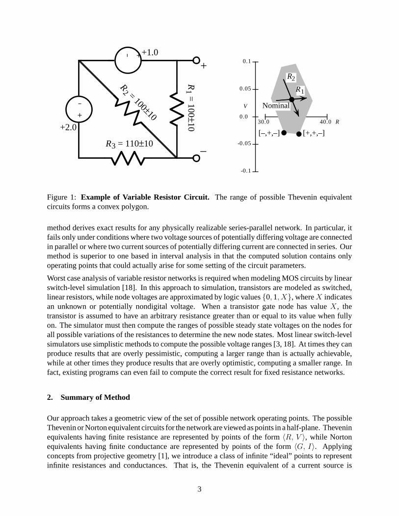
Figure 1: Example of Variable Resistor Circuit. The range of possible Thevenin equivalentcircuits forms a convex polygon.

method derives exact results for any physically realizable series-parallel network. In particular, itfails only under conditions where two voltage sources of potentially differing voltage are connectedin parallel or where two current sources of potentially differing current are connected in series. Ourmethod is superior to one based in interval analysis in that the computed solution contains onlyoperating points that could actually arise for some setting of the circuit parameters.

Worst case analysis of variable resistor networks is required when modeling MOS circuits by linearswitch-level simulation [18]. In this approach to simulation, transistors are modeled as switched,linear resistors, while node voltages are approximated by logic values {0, 1, X}, where X indicatesan unknown or potentially nondigital voltage. When a transistor gate node has value X , thetransistor is assumed to have an arbitrary resistance greater than or equal to its value when fullyon. The simulator must then compute the ranges of possible steady state voltages on the nodes forall possible variations of the resistances to determine the new node states. Most linear switch-levelsimulators use simplistic methods to compute the possible voltage ranges [3, 18]. At times they canproduce results that are overly pessimistic, computing a larger range than is actually achievable,while at other times they produce results that are overly optimistic, computing a smaller range. Infact, existing programs can even fail to compute the correct result for fixed resistance networks.

2. Summary of Method

Our approach takes a geometric view of the set of possible network operating points. The possibleThevenin or Norton equivalent circuits for the network are viewed as points in a half-plane. Theveninequivalents having finite resistance are represented by points of the form 〈R, V 〉, while Nortonequivalents having finite conductance are represented by points of the form 〈G, I〉. Applyingconcepts from projective geometry [1], we introduce a class of infinite “ideal” points to representinfinite resistances and conductances. That is, the Thevenin equivalent of a current source is

3

given by ideal point 〈〈I〉〉, while the Norton equivalent of a voltage source is given by ideal point〈〈V 〉〉. Note that unlike other geometric interpretations of optimization problems, our coordinatescorrespond to derived quantities rather than to the optimization parameters.

Our main result is to show that the Thevenin or Norton equivalent of a series-parallel networkcontaining k variable elements can be represented as a convex polygon of degree (i.e., number ofvertices) less than or equal to 2k. Furthermore, if the network contains a total of n elements, thispolygon can be computed in time O(nk). Given such a polygon, one can easily determine theranges of possible steady state voltages, currents, resistances, or conductances.

Figure 1 illustrates this approach for a circuit used in [7] to illustrate the inability of small-scalesensitivity analysis to solve the worst case analysis problem. The Thevenin representation of thecircuit across the two terminals is plotted on the right hand side of the figure. The Theveninequivalent under nominal conditions gives the point labeled “Nominal.” The lines labeled R1 andR2 illustrate the sensitivities with respect to variations in these two resistors relative to their nominalvalues. These sensitivities would seem to indicate that the minimum voltage would occur when R1

is minimized and R2 is maximized. Although not shown, sensitivity analysis also indicates that R3

should be minimized. Under these conditions we would obtain a Thevenin equivalent given by thepoint labeled [−, +,−]. Note however, that the Thevenin voltage would actually be lower by settingR1 to its maximum value, as denoted by the point labeled [+, +,−]. As this figure illustrates, therange of possible Thevenin equivalents forms a convex polygon with 6 vertices. By computingthis polygon explicitly, we can determine the extreme values of the voltage across the terminals byfinding the vertices with minimum and maximum Y values.

For the special case of a “grounded tree” network, where the circuit becomes acyclic when allbranches to ground are deleted, we can compute the polygons for every node in the tree (relative toground) by an algorithm with time complexity O(nk). This algorithm is optimal in that it generatesn polygons, each having degree up to 2k.

This algorithm could form the basis for the steady state voltage computation in a linear switch-levelsimulator. By performing series-parallel reductions on pullup and pulldown network structures,most of the channel connected components found in MOS circuits can be represented as groundedtrees. The worst case complexity would be quadratic in the number of transistors, as opposed tothe linear complexity of existing algorithms. However, this worst case complexity would only ariseunder the following conditions: (1) the channel-connected component is very large, (2) a largefraction of the transistors must be modeled as variable resistors, and (3) the achievable voltageson almost every node strongly depends on most of these variable resistances. Such a combinationwould seldom arise in practice.

3. Geometric Representation

Our geometry is based on planar projective geometry [1], where the conventional set of “Euclidean”points is augmented by a set of “ideal” points denoting the intersections of parallel lines. We restrictEuclidean points to lie in the half-plane having Cartesian coordinates with x ≥ 0. In electricalterms, this means that no negative resistances or conductances are allowed.1 Ideal points represent

1This restriction is introduced for sake of simplicity. It avoids the difficulty in projective geometry of defining anordering of points on a line—a line is viewed as “wrapping around” through its ideal point. It seems likely that our

4

+−

↑

V = 1.5 I = –0.75 R = 0.5

A B C

EUCLIDEAN IDEAL

VR1 .0 2 .0

1 .0

-1 .0

2 .0

-2 .0

1 .0

-1 .0

2 .0

-2 .0

A

B

CI

G1 .0 2 .0

1 .0

-1 .0

2 .0

-2 .0

1 .0

-1 .0

2 .0

-2 .0

A

B

C

EUCLIDEAN IDEALThevenin Representation Norton Representation

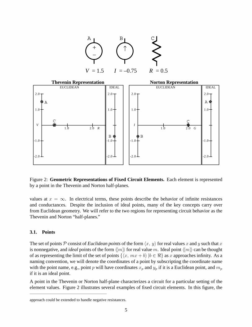
Figure 2: Geometric Representations of Fixed Circuit Elements. Each element is representedby a point in the Thevenin and Norton half-planes.

values at x = ∞. In electrical terms, these points describe the behavior of infinite resistancesand conductances. Despite the inclusion of ideal points, many of the key concepts carry overfrom Euclidean geometry. We will refer to the two regions for representing circuit behavior as theThevenin and Norton “half-planes.”

3.1. Points

The set of points P consist of Euclidean points of the form 〈x, y〉 for real values x and y such that xis nonnegative, and ideal points of the form 〈〈m〉〉 for real value m. Ideal point 〈〈m〉〉 can be thoughtof as representing the limit of the set of points {〈x, mx + b〉 |b ∈ �} as x approaches infinity. As anaming convention, we will denote the coordinates of a point by subscripting the coordinate namewith the point name, e.g., point p will have coordinates xp and yp if it is a Euclidean point, and mp

if it is an ideal point.

A point in the Thevenin or Norton half-plane characterizes a circuit for a particular setting of theelement values. Figure 2 illustrates several examples of fixed circuit elements. In this figure, the

approach could be extended to handle negative resistances.

5

half-planes are drawn with Euclidean points on the left and ideal points on a separate axis on theright. Note that the X axis for the Euclidean points actually extends indefinitely far to the right.Note also that the vertical scale for ideal points will generally differ from that for Euclidean points.A voltage source V is represented in the Thevenin half-plane by the Euclidean point 〈0, V 〉 and inNorton half-plane by the ideal point 〈〈V 〉〉. A current source I is represented in a dual way as theideal point 〈〈I〉〉 in the Thevenin half-plane and as the Euclidean point 〈0, I〉 in the Norton. Finally,a nonzero, finite resistance R is represented in the Thevenin half-plane by the Euclidean point〈R, 0〉 and in the Norton by the point 〈1/R, 0〉. Euclidean point 〈0, 0〉 is of special interest—itis the Thevenin representation of a short circuit and the Norton representation of an open circuit.Also of special interest is ideal point 〈〈0〉〉—the Thevenin representation of an open circuit and theNorton representation of a short circuit.

As notation, we will say that points p and q are ordered left to right, denoted p ≺ H q (for “Hori-zontal”) if either p is a Euclidean point while q is an ideal point, or both are Euclidean points andxp is less than xq. Similarly, we will say that p and q are vertically aligned, denoted p ≡ H q (for“horizontally equivalent”) if either both are ideal points or are Euclidean points with identical Xcoordinates. Observe that for any two points p and q, we must have either p ≺ H q, p ≡ H q, orq ≺ H p. Points p and q are ordered p H q if either p ≺ H q or p ≡ H q.

Vertically aligned points p and q are ordered vertically, denoted p < V q if either both are idealpoints and mp is less than mq, or both are Euclidean points and yp is less than yq. Note that pointsthat are not vertically aligned are considered unordered with respect to this relation. Points p andq are ordered p ≤ V q if either p < V q or p = q.

Point p is said to be between points pa and pb if one of the following sets of conditions holds. Forthe case where pa ≺ H pb, we must have pa H p H pb. For the case where pb ≺ H pa, we musthave pb H p H pa. For the case where pa ≡ H pb, we must have either pa ≤ V p ≤ V pb orpb ≤ V p ≤ V pa. Note that a point can be between two others without being colinear.

3.2. Lines

Lines in a half-plane are categorized as either “angled,” “vertical,” or “ideal,” depending on theorientation and the X coordinates. An angled line is characterized by its slope m and its Y -interceptb:

λ A (m, b) .= {〈x, mx + b〉 |x ≥ 0} ∪ {〈〈m〉〉}

A vertical line consists of all points having a given X coordinate:

λ V (x) .= {〈x, y〉 |y ∈ �}

The ideal line consists of all ideal points:

λ∞.= {〈〈m〉〉 |m ∈ �}

In comparing our geometry to Euclidean geometry, we see that angled and vertical lines correspondto the portions of lines in the plane having Cartesian coordinates with x ≥ 0, while the ideal linehas no analog. Note that unlike in Euclidean geometry, parallel lines may intersect. In particular,all angled lines with slope m contain the ideal point 〈〈m〉〉.

6

+−

↑

V = 1.25

0 ≤ R ≤ ∞I = –0.75

+−

↑

V = 1.25

0 ≤ G ≤ ∞

I = –0.75

≡

A A’

↑

G = 0.8–∞ < I < ∞+−

–∞ < V < ∞

R = 1.25

≡

B B’

VR

2 .0

-2 .0

1.25

-1.25

1 .0

-1 .0

0.75

-0.75

1.0

A

B

slope = –0.75

EUCLIDEAN IDEAL

IG

2.0

-2.0

1 .25

-1 .25

2 .0

-2 .0

0.75

-0.75

1 .0

A’

B’

slope = 1.25

EUCLIDEAN IDEAL

Angled:

Vertical:

Thevenin Representation Norton Representation

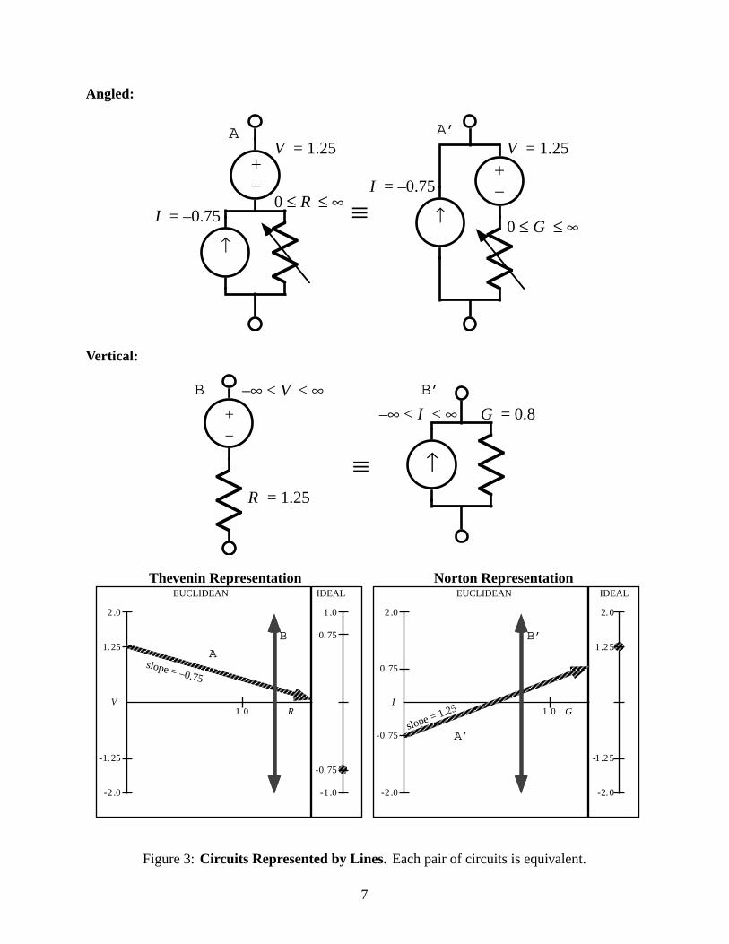
Figure 3: Circuits Represented by Lines. Each pair of circuits is equivalent.

7

In electrical terms, a line corresponds to a network containing a single variable element operatingover all possible values. Examples of circuits generating angled and vertical lines are illustratedin Figure 3. A circuit consisting of a voltage source V in series with the parallel combinationof current source I and a variable resistor with 0 ≤ R ≤ ∞ (circuit A) is represented in theThevenin half-plane by an angled line with Y -intercept V and slope I . Observe that the Theveninrepresentation of this circuit includes ideal point 〈〈I〉〉, indicating that when the resistance is infinite,the circuit reduces to a current source. As indicated in the figure, this circuit is equivalent to onewith the current source in parallel with the series connection of the voltage source and the resistor(circuit A’). Thus, the Norton representation of the circuit is also a line, but with Y -intercept Iand slope V . The Norton representation of the circuit includes the ideal point 〈〈V 〉〉, indicating thatwhen the conductance is infinite, the circuit reduces to a voltage source. A circuit consisting ofa variable voltage source with −∞ < V < ∞ in series with a fixed resistance R (circuit B) isrepresented in the Thevenin half-plane by a vertical line with X-intercept R. As indicated in thefigure, this circuit is equivalent to one with the resistor in parallel with a variable current sourcewith −∞ < I < ∞ (circuit B’). Thus, the Norton representation of the circuit is also a verticalline, but with X-intercept 1/R.

Any pair of distinct points p and q defines a line λ (p, q). The line type depends on the categoriesof the two points, and on their vertical alignment:

1. Euclidean points p = 〈xp, yp〉 and q = 〈xq, yq〉 such that xp = xq define an angled line:

λ (p, q) .= λ A

(yq − yp

xq − xp

,xqyp − xpyq

xq − xp

)

2. Euclidean point p = 〈xp, yp〉 and ideal point q = 〈〈mq〉〉 (listed in either order) define anangled line:

λ (p, q) .= λ (q, p) .

= λ A(mq, yp − mqxp

)3. Vertically aligned Euclidean points p = 〈x, yp〉 and q = 〈x, yq〉 define a vertical line:

λ (p, q) .= λ V (x).

4. Two ideal points p and q define the ideal line: λ (p, q) .= λ∞.

Distinct points pa, pb, and pc are colinear provided λ (pa, pb) = λ (pb, pc).

3.3. Segments

Two distinct points p and q define a segment [p, q] consisting of the set of all points on the lineλ (p, q) lying between the two points. These points are called the endpoints of the segment. Wewill refer to a segment as σ, σa, etc.

Relating our segments to Euclidean geometry, a segment with Euclidean endpoints correspondsto the usual definition of a line segment. For Euclidean point p and ideal point q, segment [p, q]corresponds to a ray directed to the right, with origin p and slope determined by q. The segmentformed by two ideal points has no counterpart in Euclidean geometry.

8

+−

↑

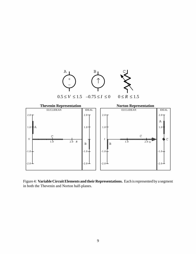
0.5 ≤ V ≤ 1.5 –0.75 ≤ I ≤ 0 0 ≤ R ≤ 1.5

A B C

VR1 .0 2 .0

1 .0

-1 .0

2 .0

-2 .0

1 .0

-1 .0

2 .0

-2 .0

A

B

C

EUCLIDEAN IDEAL

IG1 .0 2 .0

1 .0

-1 .0

2 .0

-2 .0

1 .0

-1 .0

2 .0

-2 .0

A

B

CC

EUCLIDEAN IDEAL

Thevenin Representation Norton Representation

Figure 4: Variable Circuit Elements and their Representations. Each is represented by a segmentin both the Thevenin and Norton half-planes.

9

As illustrated in Figure 4, a single, variable circuit element is represented by a segment in eitherthe Thevenin or Norton half-plane. A voltage source varying between Vmin and Vmax (circuit A) isrepresented in the Thevenin plane as a line segment along the Y axis having end points 〈0, Vmin〉 and〈0, Vmax〉 indicating that its Thevenin resistance is 0. The same source is represented in the Nortonplane as a line segment along the Ideal axis having endpoints 〈〈Vmin〉〉 and 〈〈Vmax〉〉, indicating thatit has infinite Norton conductance. The representations of a current source (circuit B) are the dualsof those for a voltage source—either a segment along the Ideal axis in the Thevenin half-plane or asegment along the Y axis in the Norton half-plane. A resistor varying from 0 to a finite value Rmax

(circuit C) is represented in both Thevenin and Norton planes as horizontal line segments alongthe X axis. In the Thevenin plane this segment has endpoints 〈0, 0〉 and 〈Rmax, 0〉, while in theNorton plane it has endpoints 〈1/Rmax, 0〉 and 〈〈0〉〉. Note that this segment includes all Euclideanpoints 〈x, 0〉 with x ≥ 1/Rmax. If this resistor had Rmax = ∞ (i.e., an open circuit), the Theveninrepresentation would still be a segment, but the right hand endpoint would be the ideal point 〈〈0〉〉and the segment would contain all Euclidean points 〈x, 0〉 for x ≥ Rmin. An angled segment withnonzero slope describes circuits such as A and A’ illustrated in Figure 3, but with the resistance orconductance operating over a more limited range.

3.4. Sets of Points

We have already introduced two types of point sets, namely lines and segments. As was discussed,these types of sets represent networks containing a single variable element. When multiple variableelements are present, we must consider more general classes of sets.

We will consider the properties of several functions operating over points, and their generalizationto functions over sets of points. For n > 0, define an n-ary point function as a mapping f :Pn → P .Such a function is generalized to one mapping n sets of points to a set of points as:

f(S1, S2, . . . , Sn).= {f(p1, p2, . . . , pn)|p1 ∈ S1, p2 ∈ S2, . . . , pn ∈ Sn}, (1)

i.e., as the union of the mappings of all of the points in the arguments. For the case where fis undefined for some combination of point arguments, we will say that the generalization to setarguments is undefined if the arguments contain any combination of points for which f is undefined.

From this definition, we can observe that such an extension must be monotonic over ⊆. That is, ifSi ⊆ Ti for all i, then f(S1, S2, . . . Sn) is defined whenever f(T1, T2, . . . Tn) is defined, and in thiscase f(S1, S2, . . . Sn) ⊆ f(T1, T2, . . . Tn). Furthermore, if f :P → P is a bijection, then so is itsextension to sets.

3.5. Point Sequences

Point sequences provide a notation for describing the upper and lower boundaries of sets. A pointsequence is a finite sequence p1, p2, . . . , pk satisfying the following two properties. First, the pointsare ordered left to right, i.e., pi H pi+1 for all 1 ≤ i < k. Second, distinct points are not verticallyaligned, i.e., if pi ≡ H pi+1, for some 1 ≤ i < k, then pi = pi+1.

Such a sequence defines a set of points consisting of the elements of the sequence, as well as those

10

in the segments connecting successive elements:

B (P ) .= {p1} ∪

⋃1≤i<k

[pi, pi+1

]

Note that {p1} is included in the equation above to cover the case where this is the only element ofP . Observe that for any q such that p1 H q H pk, there is exactly one point p in B (P ) such thatq ≡ H p. Given a point q such that p1 H q H pk, we classify this point as being either below,on, or above point sequence P according to its vertical ordering with respect to the point p in B (P )such that q ≡ H p.

A point sequence is reduced provided each element is distinct, and no 3 successive elements arecolinear. Observe that for any point sequence P , we can form a reduced sequence P ′ such thatB (P ) = B (

P ′) by simply eliminating any duplicate elements, as well as any point pi such thatpi−1, pi, and pi+1 are colinear.

Point sequence C is an upper contour (respectively, lower contour) for set S provided every elementofB (C) is in S, and every point in S lies on or below (resp., above) C. Observe that if set S has bothupper and lower contours, then the initial and final elements of these contours must be verticallyaligned.

3.6. Convex Polygons

A set S is convex if for any distinct points p and q in S, all points in the segment [p, q] are also in S.A convex polygon is a convex set S having an upper contour U and a lower contour L, both of whichare reduced. The distinct elements of U and L form the vertices of the polygon. The degree of thepolygon is the number of vertices. The edges of the polygon are the segments having as endpointssuccessive elements of U or L, as well as segments connecting the initial or final elements of Uand L, provided these are distinct. Observe that a convex polygon of degree 1 has no edges; one ofdegree 2 has a single edge; and one of degree k > 2 has k edges.

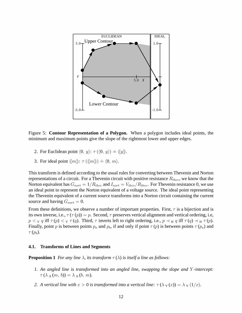
A convex polygon consisting of only Euclidean points matches the usual definition of a convexpolygon. As illustrated in Figure 5, a convex polygon containing ideal points must have points〈〈mu〉〉 and 〈〈ml〉〉 as the final points in its upper and lower contours, respectively, where ml ≤ mu

(in this example ml = mu = −0.25). Such a polygon extends infinitely to the right, having lineswith slopes ml and mu as tangents.

4. The N-T Transform

The N-T transform describes how to transform the Thevenin representation of a circuit into itsNorton equivalent, and vice versa. It can thus be viewed as a mapping over points. Operations ofthis form have been studied extensively in the field of projective geometry, where they are used tocreate a perspective drawing of an image [17].

Define the function τ :P → P as:

1. For Euclidean point 〈x, y〉 with x > 0: τ(〈x, y〉) .

= 〈1/x, y/x〉.

11

YX5.0

5.0

-5.0

1.0

-1.0

Upper Contour

Lower Contour

EUCLIDEAN IDEAL

Figure 5: Contour Representation of a Polygon. When a polygon includes ideal points, theminimum and maximum points give the slope of the rightmost lower and upper edges.

2. For Euclidean point 〈0, y〉: τ(〈0, y〉) .

= 〈〈y〉〉.

3. For ideal point 〈〈m〉〉: τ(〈〈m〉〉) .

= 〈0, m〉.

This transform is defined according to the usual rules for converting between Thevenin and Nortonrepresentations of a circuit. For a Thevenin circuit with positive resistance Rthev, we know that theNorton equivalent has Gnort = 1/Rthev and Inort = Vthev/Rthev. For Thevenin resistance 0, we usean ideal point to represent the Norton equivalent of a voltage source. The ideal point representingthe Thevenin equivalent of a current source transforms into a Norton circuit containing the currentsource and having Gnort = 0.

From these definitions, we observe a number of important properties. First, τ is a bijection and isits own inverse, i.e., τ (τ (p)) = p. Second, τ preserves vertical alignment and vertical ordering, i.e,p < V q iff τ (p) < V τ (q). Third, τ inverts left to right ordering, i.e., p ≺ H q iff τ (q) ≺ H τ (p).Finally, point p is between points pa and pb, if and only if point τ (p) is between points τ (pa) andτ (pb).

4.1. Transforms of Lines and Segments

Proposition 1 For any line λ, its transform τ (λ) is itself a line as follows:

1. An angled line is transformed into an angled line, swapping the slope and Y -intercept:τ (λ A (m, b)) = λ A (b, m).

2. A vertical line with x > 0 is transformed into a vertical line: τ (λ V (x)) = λ V(1/x

).

12

3. The vertical line with x = 0 is transformed into the ideal line: τ (λ V (0)) = λ∞.

4. The ideal line is transformed to the vertical line with x = 0: τ (λ∞) = λ V (0).

Proof: For the case of an angled line, observe that for any Euclidean point p = 〈x, mx + b〉 withx > 0, its transform is given by: τ (p) = 〈1/x, b/x + m〉 = 〈x′, bx′ + m〉, for the substitutionx′ = 1/x, and hence the transformed point lies on the angled line with slope b and Y -intercept m.Furthermore, as x ranges over all positive real values, we see that x′ also ranges over all positive realvalues. Finally, points 〈0, b〉 and 〈〈m〉〉 have as transforms 〈〈b〉〉 and 〈0, m〉, respectively, completingthe mapping to the line λ A (b, m).

The other 3 cases follow directly from the definition of the transform.

The property that the transform of an angled line is itself an angled line can be understood inelectrical terms by the examples of circuits A and A’ in Figure 3. These circuits are equivalent andeach is represented by an angled line in its respective half-plane.

Proposition 2 The transform of a segment [p, q] is given by the segment having τ (p) and τ (q) asits endpoints.

Proof: Having shown that the transform of a line is itself a line, we know that τ (λ (p, q)) =λ (τ (p) , τ (q)). From this we can conclude that τ ([p, q]) ⊆ λ (τ (p) , τ (q)). Furthermore, a pointis between points p and q if and only if its transform is between points τ (p) and τ (q). From thiswe can conclude that τ ([p, q]) = [τ (p) , τ (q)].

For a segment σ, we will denote its transform as τ (σ), bearing in mind that τ (σ) is itself a segmenthaving as endpoints the transformed endpoints of σ.

4.2. Transforms of Sets and Polygons

Many properties of sets are preserved under the transform operator. Note also that in order to provea statement of the form “Property P holds for a set S if and only if P holds for the set τ (S),” itsuffices to give the proof in one direction. For example, suppose we prove the statement “If Pholds for S then P holds for τ (S).” Then the converse follows by substituting τ (S) for S in theantecedent, and τ (τ (S)) = S for τ (S) in the consequent.

Lemma 1 Set S is convex if and only if τ (S) is convex.

Proof: We will prove the “if” direction, i.e., that if τ (S) is convex then S is convex.

Suppose that set τ (S) is convex. For any points p and q in S, their transforms, τ (p) and τ (q) arein τ (S), and hence by convexity, any point in the segment [τ (p) , τ (q)] is also in τ (S). We knowthat this segment is the transform of the segment [p, q], and hence any point in the segment [p, q]is in S.

13

Lemma 2 Sequence P = p1, p2, . . . , pk is a reduced point sequence if and only if sequence τ (P ) .=

τ (pk) , τ (pk−1) , . . . , τ (p1) is a reduced point sequence.

Proof: We will prove the “only if” direction. Clearly, τ (P ) is a point sequence, since the transformoperator maintains vertical alignment and reverses left to right ordering. Furthermore, if successiveelements of P are distinct, then their transforms are also distinct. We can see that no three successivepoints in τ (P ) can be colinear, because otherwise the corresponding elements in P would also becolinear.

Lemma 3 τ (B (P )) = B (τ (P )), for any point sequence P .

Proof: This follows by the definition of B (P ) and the fact that the transform operator applies tosegments.

Lemma 4 If C is an upper (respectively, lower) contour for S, then τ (C) is an upper (resp., lower)contour for τ (S).

Proof: We have just shown that τ (B (C)) = B (τ (C)), and hence every point in B (τ (C)) is inτ (S). Furthermore, the transform operator preserves vertical alignment and vertical ordering, andhence if point p is on or below (resp., above) C, then τ (p) is on or below (resp., above) τ (C).

Theorem 1 S is a convex polygon of degree k if and only if τ (S) is also a convex polygon of degreek.

Proof: Given that S is a convex set with upper and lower contours U and L, we can see that τ (S)is a convex set having upper and lower contours τ (U ) and τ (L).

Given a representation of a convex polygon in terms of its upper and lower contours, we can easilycompute the transform of this polygon. The upper and lower contours of the new polygon arecomputed by simply applying the transform operator to each element in the original contours,while reversing the ordering of elements in the two sequences.

5. Point Addition

Point addition describes the effect of combining networks in series (given their Thevenin represen-tations) and in parallel (given their Norton representations).

For points p and q their sum, denoted p + q is defined as:

1. For Euclidean points p = 〈xp, yp〉 and q = 〈xq, yq〉: p + q.= 〈xp + xq, yp + yq〉.

14

pa

qa

pb

qb

pa + pb

qa + qb

σa

σb

σa + σb

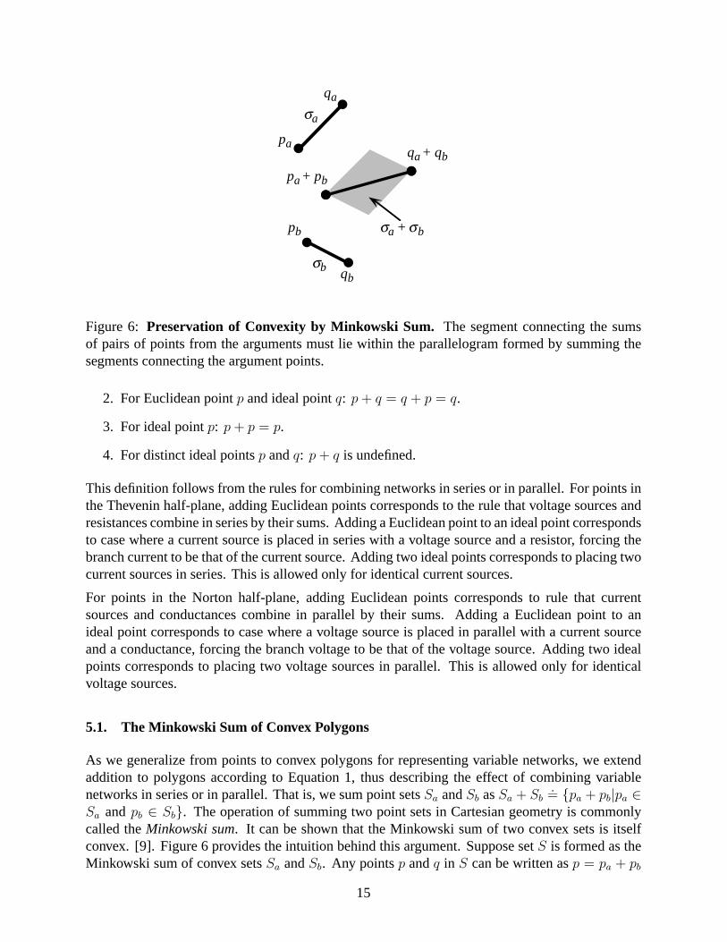
Figure 6: Preservation of Convexity by Minkowski Sum. The segment connecting the sumsof pairs of points from the arguments must lie within the parallelogram formed by summing thesegments connecting the argument points.

2. For Euclidean point p and ideal point q: p + q = q + p = q.

3. For ideal point p: p + p = p.

4. For distinct ideal points p and q: p + q is undefined.

This definition follows from the rules for combining networks in series or in parallel. For points inthe Thevenin half-plane, adding Euclidean points corresponds to the rule that voltage sources andresistances combine in series by their sums. Adding a Euclidean point to an ideal point correspondsto case where a current source is placed in series with a voltage source and a resistor, forcing thebranch current to be that of the current source. Adding two ideal points corresponds to placing twocurrent sources in series. This is allowed only for identical current sources.

For points in the Norton half-plane, adding Euclidean points corresponds to rule that currentsources and conductances combine in parallel by their sums. Adding a Euclidean point to anideal point corresponds to case where a voltage source is placed in parallel with a current sourceand a conductance, forcing the branch voltage to be that of the voltage source. Adding two idealpoints corresponds to placing two voltage sources in parallel. This is allowed only for identicalvoltage sources.

5.1. The Minkowski Sum of Convex Polygons

As we generalize from points to convex polygons for representing variable networks, we extendaddition to polygons according to Equation 1, thus describing the effect of combining variablenetworks in series or in parallel. That is, we sum point sets Sa and Sb as Sa + Sb

.= {pa + pb|pa ∈

Sa and pb ∈ Sb}. The operation of summing two point sets in Cartesian geometry is commonlycalled the Minkowski sum. It can be shown that the Minkowski sum of two convex sets is itselfconvex. [9]. Figure 6 provides the intuition behind this argument. Suppose set S is formed as theMinkowski sum of convex sets Sa and Sb. Any points p and q in S can be written as p = pa + pb

15

Sa + Sb

pa + pb

Sa

pa

Sb

pb

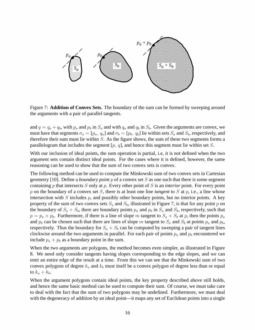
Figure 7: Addition of Convex Sets. The boundary of the sum can be formed by sweeping aroundthe arguments with a pair of parallel tangents.

and q = qa + qb, with pa and pb in Sa and with qa and qb in Sb. Given the arguments are convex, wemust have that segments σa = [pa, qa] and σb = [pb, qb] lie within sets Sa and Sb, respectively, andtherefore their sum must lie within S. As the figure shows, the sum of these two segments forms aparallelogram that includes the segment [p, q], and hence this segment must lie within set S.

With our inclusion of ideal points, the sum operation is partial, i.e, it is not defined when the twoargument sets contain distinct ideal points. For the cases where it is defined, however, the samereasoning can be used to show that the sum of two convex sets is convex.

The following method can be used to compute the Minkowski sum of two convex sets in Cartesiangeometry [10]. Define a boundary point p of a convex set S as one such that there is some segmentcontaining p that intersects S only at p. Every other point of S is an interior point. For every pointp on the boundary of a convex set S, there is at least one line tangent to S at p, i.e., a line whoseintersection with S includes p, and possibly other boundary points, but no interior points. A keyproperty of the sum of two convex sets Sa and Sb, illustrated in Figure 7, is that for any point p onthe boundary of Sa + Sb, there are boundary points pa and pb in Sa and Sb, respectively, such thatp = pa + pb. Furthermore, if there is a line of slope m tangent to Sa + Sb at p, then the points pa

and pb can be chosen such that there are lines of slope m tangent to Sa and Sb at points pa and pb,respectively. Thus the boundary for Sa + Sb can be computed by sweeping a pair of tangent linesclockwise around the two arguments in parallel. For each pair of points pa and pb encountered weinclude pa + pb as a boundary point in the sum.

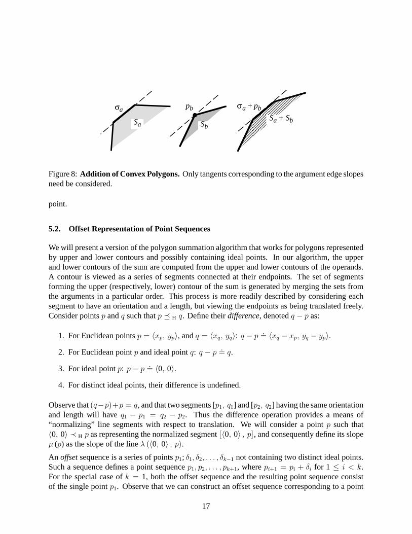
When the two arguments are polygons, the method becomes even simpler, as illustrated in Figure8. We need only consider tangents having slopes corresponding to the edge slopes, and we canemit an entire edge of the result at a time. From this we can see that the Minkowski sum of twoconvex polygons of degree ka and kb must itself be a convex polygon of degree less than or equalto ka + kb.

When the argument polygons contain ideal points, the key property described above still holds,and hence the same basic method can be used to compute their sum. Of course, we must take careto deal with the fact that the sum of two polygons may be undefined. Furthermore, we must dealwith the degeneracy of addition by an ideal point—it maps any set of Euclidean points into a single

16

Sa

σa

Sb

pb

Sa + Sb

σa + pb

Figure 8: Addition of Convex Polygons. Only tangents corresponding to the argument edge slopesneed be considered.

point.

5.2. Offset Representation of Point Sequences

We will present a version of the polygon summation algorithm that works for polygons representedby upper and lower contours and possibly containing ideal points. In our algorithm, the upperand lower contours of the sum are computed from the upper and lower contours of the operands.A contour is viewed as a series of segments connected at their endpoints. The set of segmentsforming the upper (respectively, lower) contour of the sum is generated by merging the sets fromthe arguments in a particular order. This process is more readily described by considering eachsegment to have an orientation and a length, but viewing the endpoints as being translated freely.Consider points p and q such that p H q. Define their difference, denoted q − p as:

1. For Euclidean points p = 〈xp, yp〉, and q = 〈xq, yq〉: q − p.= 〈xq − xp, yq − yp〉.

2. For Euclidean point p and ideal point q: q − p.= q.

3. For ideal point p: p − p.= 〈0, 0〉.

4. For distinct ideal points, their difference is undefined.

Observe that (q−p)+p = q, and that two segments [p1, q1] and [p2, q2] having the same orientationand length will have q1 − p1 = q2 − p2. Thus the difference operation provides a means of“normalizing” line segments with respect to translation. We will consider a point p such that〈0, 0〉 ≺ H p as representing the normalized segment

[〈0, 0〉 , p], and consequently define its slope

µ (p) as the slope of the line λ(〈0, 0〉 , p

).

An offset sequence is a series of points p1; δ1, δ2, . . . , δk−1 not containing two distinct ideal points.Such a sequence defines a point sequence p1, p2, . . . , pk+1, where pi+1 = pi + δi for 1 ≤ i < k.For the special case of k = 1, both the offset sequence and the resulting point sequence consistof the single point p1. Observe that we can construct an offset sequence corresponding to a point

17

sequence by letting δi.= pi+1 − pi for 1 ≤ i < k. Thus, we will view an offset sequence as an

alternative representation of a point sequence.

An offset sequence defines a reduced point sequence if and only if the following properties hold:

1. There are no elements of the form δi = 〈0, 0〉.

2. If point p1 is an ideal point, then k = 1.

3. Point δi is not an ideal point for any i < k − 1.

4. There are no successive points δi−1 and δi such that µ (δi−1) = µ (δi).

Observe that an offset sequence can be reduced by eliminating any elements of the form δi = 〈0, 0〉,by eliminating any elements beyond an ideal point, and by replacing any pair of elements δi−1 and δi

for which µ (δi−1) = µ (δi) by the single element δi−1 + δi. This reduction is equivalent to reducingthe corresponding point sequence.

A reduced point sequence having offset representationp1; δ1, δ2, . . . , δk−1 is said to be convex upward(respectively, downward), provided µ (δi−1) > µ (δi) (resp., µ (δi−1) < µ (δi)) for all 1 < i < k.An arbitrary point sequence is convex upward (resp., downward), if its reduction is convex upward(resp., downward).

5.3. Addition of Polygons

Given two convex polygons Sa and Sb the following algorithm computes the upper and lowercontours of the sum Sa + Sb from the upper and lower contours of Sa and Sb. Suppose thatreduced point sequences A and B are the upper contours for Sa and Sb, respectively. Thesecontours are convex upward. Let their offset sequence representations be a1; α1, α2, . . . , αka−1, andb1; β1, β2, . . . , βkb−1, respectively. Their convex upward sum, denoted A

�+ B is defined as long as

αka−1 and βkb−1 are not distinct ideal points. This sum is the point sequence having offset sequencerepresentation a1 + b1, δ1, δ2, . . . , δka+kb−2 where the sequence δ1, . . . δka+kb−2 is an interleavingof the sequences α1, . . . , αka−1 and β1, . . . , βkb−1, such that δi−1 ≥ δi for 1 < i ≤ ka + kb − 2.In computing this sum, we effectively implement the tangent sweeping method described earlierfor the upper boundary of the sum of two convex polygons. The interleaving of argument edgesegments in decreasing order of slope matches the order edges would be encountered if we startedwith vertical lines at the left hand sides of the arguments and swept clockwise until the tangentswere vertical lines on the right hand sides of the arguments. Thus A

�+ B forms the upper contour

for Sa + Sb.

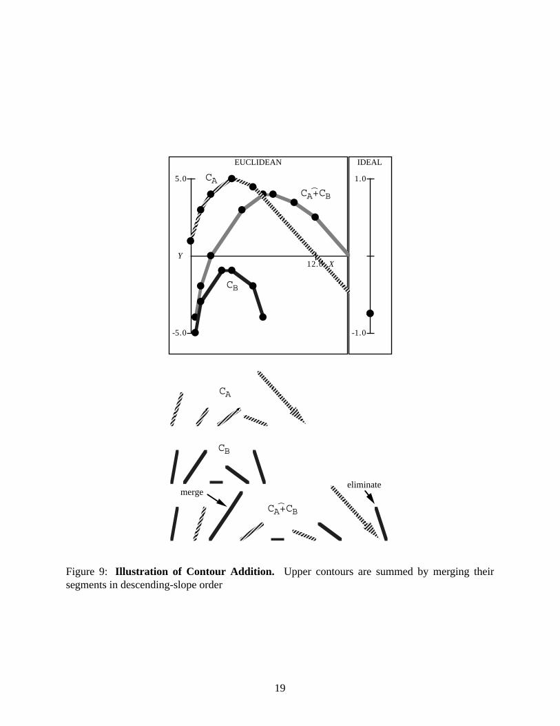
Figure 9 illustrates the process of adding two contours. The upper part of the figure shows theargument contours CA and CB, as well as their sum CA

�+ CB following its reduction. The lower

shows how this reduced sum is computed. First, the two argument contours are converted intosegment lists in descending-slope order. Next, these segments are merged into a single list. Thislist represents the contour CA

�+ Cb. We can compute a reduced sum by simply merging any

segments having equal slope (e.g., the case labeled “merge”) and by eliminating any segmentsbeyond the first ideal point (e.g., the case labeled “eliminate”).

18

EUCLIDEAN IDEAL

YX12.0

5.0

-5.0

1.0

-1.0

CA

CB

CA+CB

)

CA

CB

eliminatemerge

CA+CB

)

Figure 9: Illustration of Contour Addition. Upper contours are summed by merging theirsegments in descending-slope order

19

For convex downward point sequences A and B, their convex downward sum, denoted A�+ B, is

defined under the same conditions and in the same fashion, but with the offset elements orderedδi−1 ≤ δi. Clearly, A

�+ B is convex downward. If A and B are lower contours for convex sets Sa

and Sb such that Sa + Sb is defined, then A�+ B is the lower contour for Sa + Sb. Observe that

computing this sum implements the tangent sweeping for the lower boundary, where the tangentsstart at the left hand sides and sweep counterclockwise to the right hand sides.

These results yield an efficient algorithm for computing the sum of a convex polygon having upperand lower contours Ua and La with a convex polygon having upper and lower contours Ub and Lb.First, we determine if the sum is defined, by comparing the final elements of contours Ua and Lb

as well as those of contours La and Ub. If either of these pairs consist of distinct ideal points, thenthe sum is not defined.2 Otherwise, compute the upper contour as the reduction of Ua

�+ Ub, and

the lower contour as the reduction of La

�+ Lb. For argument polygons of degrees ka and kb, this

algorithm has complexity O(ka + kb), and the resulting polygon has degree less than or equal toka + kb.

6. Network Analysis

Now that we have developed methods to characterize Thevenin and Norton equivalents, we canreturn our attention to the task of analyzing the extreme operating conditions of a circuit.

6.1. Single Node Analysis

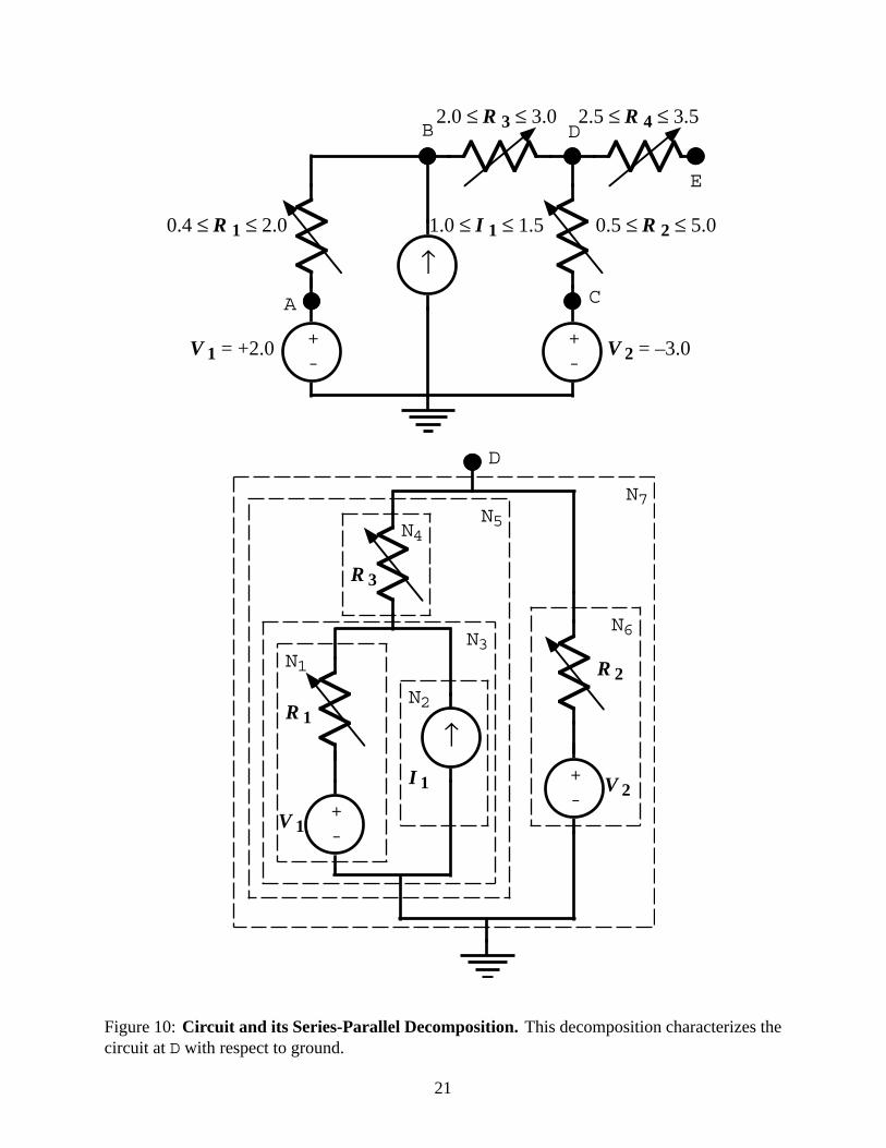
Our algorithms for the geometric transform and polygon addition operations form the basis of anetwork analysis technique for series-parallel networks. This technique is illustrated for the circuitof Figure 10 to characterize the range of possible behaviors at node D with respect to ground.First, we must decompose the circuit into a series-parallel structure with one terminal being thenode of interest, and the other being ground, as shown in the lower part of the figure. In thisdecomposition, the intermediate subnetworks are referred to as N1 through N7. Based on thisseries-parallel decomposition, we derive the Thevenin and Norton polygons by a sequence ofgeometric operations, as illustrated in Figure 11. Note that in this figure, the polygons labeled Ni

and Ti show the Norton and Thevenin representations for subnetwork Ni. Observe that at eachstep we convert to a Thevenin representation for combining subnetworks in series and to a Nortonrepresentation for combining subnetworks in parallel.

Assume the circuit contains a total of n elements, of which k are variable. The k variable elementsare represented by polygons of degree 2, while the fixed elements are represented by single points.Each time two polygons are summed, the resulting polygon has degree less than or equal to thesum of the argument degrees. For the special case where one of the arguments is a single point,the resulting polygon has degree less than or equal to the degree of the other argument. The N-Ttransform operator produces a polygon with the same degree as its argument. Thus, the polygondescribing the entire network has degree at most 2k. In the circuit of Figure 10, for example, the

2Note that just these two comparisons are sufficient—we can detect whether the right hand boundaries containdistinct ideal points by comparing the maximum of one with the minimum of the other, and vice-versa.

20

+-

+-

↑A

B

C

D

E

0.4 ≤ R 1 ≤ 2.0

V 1 = +2.0

1.0 ≤ I 1 ≤ 1.5

V 2 = –3.0

0.5 ≤ R 2 ≤ 5.0

2.0 ≤ R 3 ≤ 3.0 2.5 ≤ R 4 ≤ 3.5

+-

+-

↑R 1

V 1

I 1 V 2

R 2

R 3

D

N1

N2

N3

N4N5

N6

N7

Figure 10: Circuit and its Series-Parallel Decomposition. This decomposition characterizes thecircuit at D with respect to ground.

21

T 1

T 3

T 5

T 6

N 1

N 3

N 5

N 6

N 7

N 2

T 4

T 7

Figure 11: Derivation of Thevenin and Norton Representations for Example Circuit. Thederivation follows the series-parallel decomposition.

final result is a pair (Thevenin and Norton) of polygons of degree 6, slightly less than the maximumdegree of 8 achievable for a circuit with 4 variable elements.

The series-parallel decomposition of an n-element circuit can be represented as a tree with nleaves (corresponding to the elements), n− 1 internal nodes (each representing a series or parallelcombination), and 2(n − 1) edges. To construct the Norton or Thevenin representation of such anetwork requires at most n−1 addition operations (one per internal tree node), and 2n−1 transformoperations (one per edge, plus one at the root). For a network with k variable elements, no polygonhas more than 2k vertices, and hence each polygon operation has time complexity O(k). Therefore,the worst case complexity of analyzing such a circuit is O(nk), which in turn is at worst O(n2).

6.2. Grounded Tree Networks

In potential applications of this analysis, we may wish to characterize the range of behaviors formultiple circuit nodes. One approach would be to derive a series-parallel decomposition for everynode with respect to ground and analyze each such case separately. This approach would haveworst case complexity O(n2k) to analyze all nodes in a network with n elements of which k arevariable. On closer inspection one finds that much of this complexity is due to repeated analysis ofthe subnetworks.

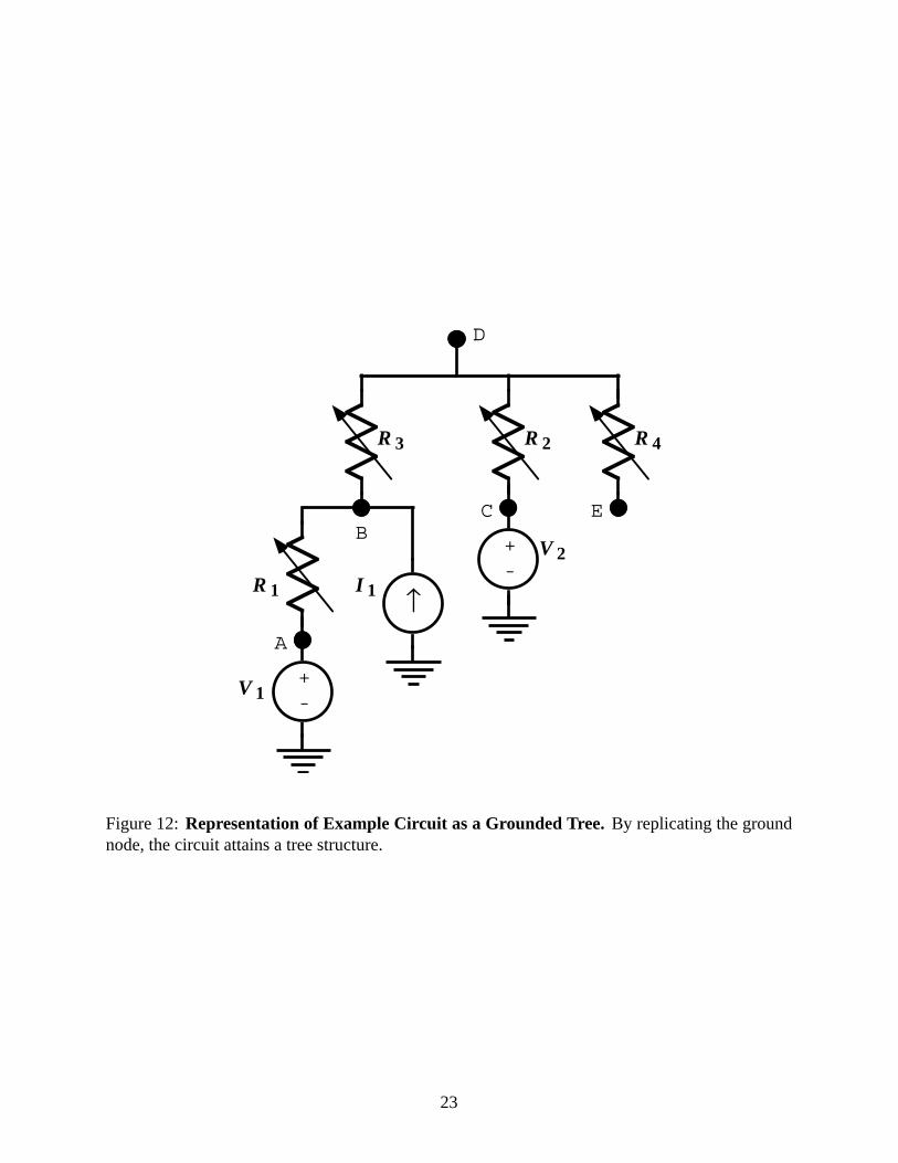
For the special case of “grounded tree” networks, we can exploit the circuit structure to analyze thecircuits for all nodes in time O(nk). This class of networks obeys the following restriction: thecircuit graph becomes acyclic when all branches connected to ground are eliminated. By selectingan arbitrary node as root, such a circuit can be drawn as a tree, where the ground node is replicatedfor each connected branch. Figure 12 illustrates the tree structure for the example circuit shown inFigure 10. This class of circuits also has the property that for every node in the circuit there is a

22

+-

+-

V 2

R 2 R 4

C E

↑R 1

V 1

I 1

R 3

D

B

A

Figure 12: Representation of Example Circuit as a Grounded Tree. By replicating the groundnode, the circuit attains a tree structure.

23

+-

+-

↑R 1

V 1

I 1

V 2

R 2

R 3

D

R 4

B

A C E

R = 0

R =

∞

R =

∞

R =

∞

R =

∞

Figure 13: Transformation of Circuit into Binary Tree. High degree nodes are split and connectedby perfect conductors, while low degree nodes are connected to ground by insulators.

24

series-parallel decomposition for the node with respect to ground.

In developing an algorithm for grounded-tree circuits, we can make simplifying assumptions aboutthe tree representation of the circuit. These assumptions simplify the presentation without affectingthe asymptotic complexity of the algorithm. In particular, we can assume that every node exceptground has exactly two children, which we will denote as LeftChild and RightChild. Such a treecorresponds to a circuit in which the root node Root has exactly two branches while all others havethree. We can transform the circuit into such a representation by splitting any nodes of higherdegree into multiple nodes connected by resistors with resistance 0. In addition, any nodes of lowerdegree can be augmented with branches to ground having infinite resistance. Figure 13 illustratesthe binary representation of our example circuit. Assuming the original circuit had n elements, itcan be seen that splitting the high degree nodes will involve adding at most n − 1 resistors, whileexpanding the low degree nodes will involve adding at most 2n resistors.3 Hence, both the numberof branches and the number of nodes in the transformed circuit will be O(n).

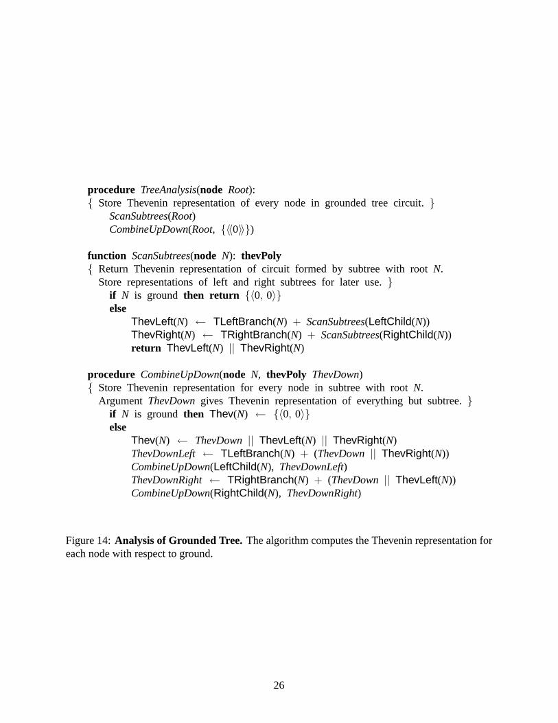
Figure 14 shows pseudo-code (following the stylistic conventions of [15]) for the grounded treeanalysis algorithm. This code computes the Thevenin representation for every node N with respect toground and stores the result as Thev(N). Alternatively, a similar technique could be used to computethe Norton representations. The code expresses the algorithm in terms of a data type thevPoly,with operations + and ||. The + operation denotes polygon addition and hence computes theseries combination of Thevenin circuits. The || operation is defined for polygons P1 and P2 asP1 ||P2

.= τ (τ (P1) + τ (P2)) and hence computes the parallel combination of Thevenin circuits.

The thevPoly representations of a short and an open circuit are given as {〈0, 0〉} and {〈〈0〉〉},respectively.

The code assumes that the Thevenin representation of each circuit element has been computedand stored as TLeftBranch(N) or TRightBranch(N), according to whether the element connectsN to its left or its right child. The algorithm operates by traversing the circuit tree twice byrecursive routines ScanSubtrees and CombineUpDown. During the first traversal it computes theThevenin representations of every subtree in the circuit. For node N, it stores intermediate resultsThevLeft(N) and ThevRight(N), giving the Thevenin representation of each of its subtree in serieswith the connecting element. It returns the parallel combination of these two intermediate valuesas the Thevenin representation of the entire subtree. During the second traversal, it combinesthese intermediate results with the Thevenin representation of the rest of the circuit, passed asthe parameter ThevDown to compute the final value for node N. It then continues the traversalby recursively calling the procedure for its two children. When making each call it computes theThevenin representation for the rest of the circuit with respect to each child.

Observe that, with the exception of ground, a given node N is “visited” by each of the recursiveroutines exactly once. Each such visit involves only a constant number of polygon operations.Hence, the overall complexity of the algorithm is O(nk) for a network with n elements of which kare variable.

Figure 15 shows the Thevenin and Norton representations of all nodes in the example circuit,computed by the grounded tree analysis algorithm. Observe that the Thevenin representations

3An example of a network that approaches this worst case would be a “star” consisting of n − 1 “leaf” nodes withbranches to a single “root” node. Splitting the root would require adding n − 2 branches, while expanding the leaveswould require adding 2 branches each.

25

procedure TreeAnalysis(node Root):{ Store Thevenin representation of every node in grounded tree circuit. }

ScanSubtrees(Root)CombineUpDown(Root, {〈〈0〉〉})

function ScanSubtrees(node N): thevPoly{ Return Thevenin representation of circuit formed by subtree with root N.

Store representations of left and right subtrees for later use. }if N is ground then return {〈0, 0〉}else

ThevLeft(N) ← TLeftBranch(N) + ScanSubtrees(LeftChild(N))ThevRight(N) ← TRightBranch(N) + ScanSubtrees(RightChild(N))return ThevLeft(N) || ThevRight(N)

procedure CombineUpDown(node N, thevPoly ThevDown){ Store Thevenin representation for every node in subtree with root N.

Argument ThevDown gives Thevenin representation of everything but subtree. }if N is ground then Thev(N) ← {〈0, 0〉}else

Thev(N) ← ThevDown || ThevLeft(N) || ThevRight(N)ThevDownLeft ← TLeftBranch(N) + (ThevDown || ThevRight(N))CombineUpDown(LeftChild(N), ThevDownLeft)ThevDownRight ← TRightBranch(N) + (ThevDown || ThevLeft(N))CombineUpDown(RightChild(N), ThevDownRight)

Figure 14: Analysis of Grounded Tree. The algorithm computes the Thevenin representation foreach node with respect to ground.

26

VR

2 .0

-2 .0

4 .0

-4 .0

2.0 4 .0 6.0

A

B

C

D E

EUCLIDEAN IDEAL

IG

3 .0

-3 .0

-6 .0

1.0 2 .0 3.0

AB

C

D

E

EUCLIDEAN IDEAL

Thevenin Representation Norton Representation

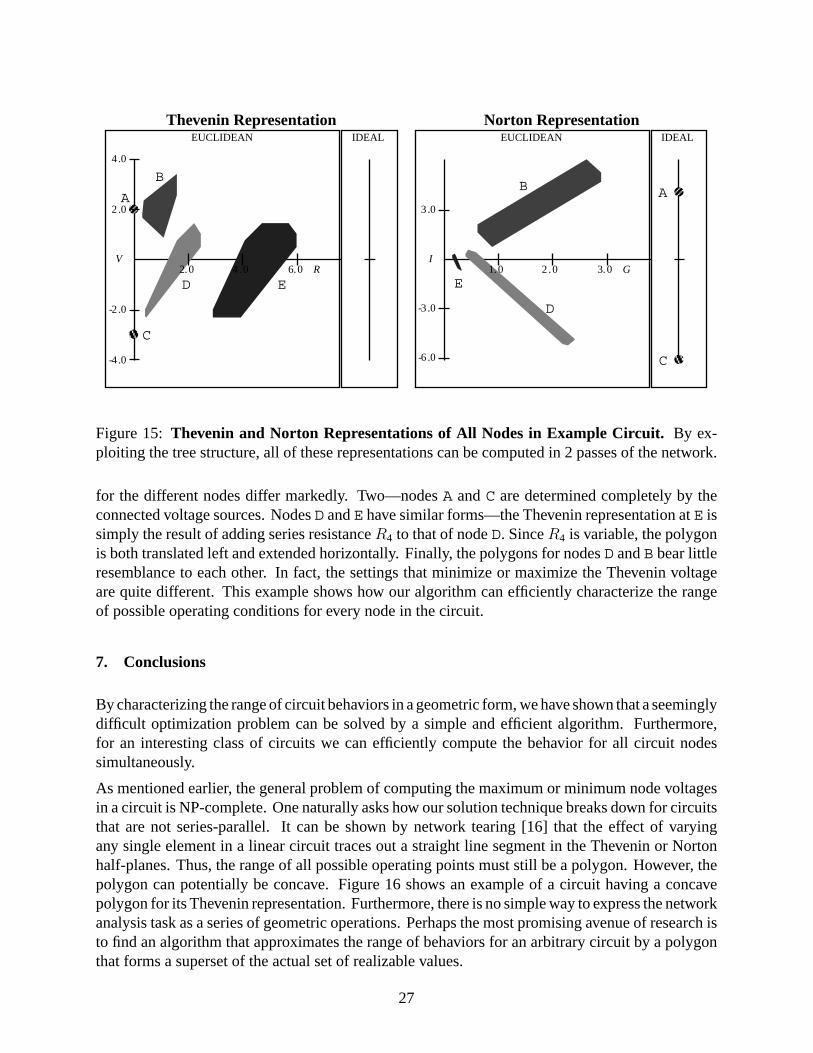
Figure 15: Thevenin and Norton Representations of All Nodes in Example Circuit. By ex-ploiting the tree structure, all of these representations can be computed in 2 passes of the network.

for the different nodes differ markedly. Two—nodes A and C are determined completely by theconnected voltage sources. Nodes D and E have similar forms—the Thevenin representation at E issimply the result of adding series resistance R4 to that of node D. Since R4 is variable, the polygonis both translated left and extended horizontally. Finally, the polygons for nodes D and B bear littleresemblance to each other. In fact, the settings that minimize or maximize the Thevenin voltageare quite different. This example shows how our algorithm can efficiently characterize the rangeof possible operating conditions for every node in the circuit.

7. Conclusions

By characterizing the range of circuit behaviors in a geometric form, we have shown that a seeminglydifficult optimization problem can be solved by a simple and efficient algorithm. Furthermore,for an interesting class of circuits we can efficiently compute the behavior for all circuit nodessimultaneously.

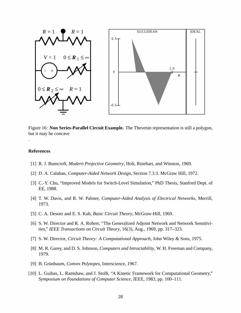
As mentioned earlier, the general problem of computing the maximum or minimum node voltagesin a circuit is NP-complete. One naturally asks how our solution technique breaks down for circuitsthat are not series-parallel. It can be shown by network tearing [16] that the effect of varyingany single element in a linear circuit traces out a straight line segment in the Thevenin or Nortonhalf-planes. Thus, the range of all possible operating points must still be a polygon. However, thepolygon can potentially be concave. Figure 16 shows an example of a circuit having a concavepolygon for its Thevenin representation. Furthermore, there is no simple way to express the networkanalysis task as a series of geometric operations. Perhaps the most promising avenue of research isto find an algorithm that approximates the range of behaviors for an arbitrary circuit by a polygonthat forms a superset of the actual set of realizable values.

27

+−

R = 1 R = 1

V = 1

R = 1

0 ≤ R 1 ≤ ∞

0 ≤ R 2 ≤ ∞

VR

2.0

0.5

-0.5

EUCLIDEAN IDEAL

Figure 16: Non Series-Parallel Circuit Example. The Thevenin representation is still a polygon,but it may be concave.

References

[1] R. J. Bumcroft, Modern Projective Geometry, Holt, Rinehart, and Winston, 1969.

[2] D. A. Calahan, Computer-Aided Network Design, Section 7.3.3. McGraw Hill, 1972.

[3] C.-Y. Chu, “Improved Models for Switch-Level Simulation,” PhD Thesis, Stanford Dept. ofEE, 1988.

[4] T. W. Davis, and R. W. Palmer, Computer-Aided Analysis of Electrical Networks, Merrill,1973.

[5] C. A. Desoer and E. S. Kuh, Basic Circuit Theory, McGraw-Hill, 1969.

[6] S. W. Director and R. A. Rohrer, “The Generalized Adjoint Network and Network Sensitivi-ties,” IEEE Transactions on Circuit Theory, 16(3), Aug., 1969, pp. 317–323.

[7] S. W. Director, Circuit Theory: A Computational Approach, John Wiley & Sons, 1975.

[8] M. R. Garey, and D. S. Johnson, Computers and Intractability, W. H. Freeman and Company,1979.

[9] B. Grunbaum, Convex Polytopes, Interscience, 1967.

[10] L. Guibas, L. Ramshaw, and J. Stolfi, “A Kinetic Framework for Computational Geometry,”Symposium on Foundations of Computer Science, IEEE, 1983, pp. 100–111.

28

[11] I. N. Hajj, “Algorithms for Solution Updating Due to Large Changes in System Parameters,”International Journal of Circuit Theory and Applications, 9(1), Jan., 1981, pp. 1–14.

[12] L. P. Huang, “Modeling Uncertainty in Linear Switch-Level Simulation,” PhD Thesis,Carnegie Mellon University Dept. of Electrical and Computer Engineering, 1991.

[13] L. P. Huang, and R. E. Bryant, “Intractability and Switch-Level Simulation,” IEEE Trans-actions on Computer-Aided Design of Integrated Circuits and Systems, 12 (6), June, 1993,pp. 829–836.

[14] K. H. Leung, and R. Spence, “Multiparameter Large-Change Sensitivity Analysis and Sys-tematic Exploration,” IEEE Transactions on Circuits and Systems, CAS-22(10), Oct., 1975,pp. 796–804.

[15] H. R. Lewis, and L. Denenberg, Data Structures and their Algorithms, HarperCollins, 1991.

[16] R. A. Rohrer, “Circuit Partitioning Simplified,” IEEE Transactions on Circuits and Systems,CAS-35(1), Jan., 1988, pp. 2–5.

[17] W. F. Taylor, The Geometry of Computer Graphics, Chapter 4, Wadsworth and Brooks/Cole,1992.

[18] C. J. Terman, “Simulation Tools for Digital LSI Design,” PhD Thesis, MIT Dept. of ElectricalEngineering and Computer Science, 1983.

[19] C. A. Zukowski, The Bounding Approach to VLSI Circuit Simulation, Kluwer, 1986.

29