geoinformatics - tankonyvtar.hu by xmlmind xsl-fo converter. geoinformatics prof. tamás, jános...
TRANSCRIPT

Created by XMLmind XSL-FO Converter.
Geoinformatics
Prof. Tamás, János
Fórián, Tünde

Created by XMLmind XSL-FO Converter.
Geoinformatics: Prof. Tamás, János Fórián, Tünde
Publication date 2011 Szerzői jog © 2011 Debreceni Egyetem. Agrár- és Gazdálkodástudományok Centruma

iii Created by XMLmind XSL-FO Converter.
Tartalom
............................................................................................................................................................ v 1. Introduction .................................................................................................................................... 1
1. .............................................................................................................................................. 1 2. 1. Base components of GIS ................................................................................................... 1
2.1. 1.1. Vector data ......................................................................................................... 2 2.2. 1.2. Raster data ......................................................................................................... 3 2.3. 1.3. Geospatial innovation ........................................................................................ 5
2. 2. Geographic and projected coordinate system ............................................................................. 7 1. .............................................................................................................................................. 7
1.1. Practice 1: Define coordinate system in ArcGIS ...................................................... 9 1.1.1. Exercise 1.1. ................................................................................................. 9 1.1.2. Exercise 1.2. ............................................................................................... 10
1.2. Practice 2: Rectify an image map to EOV coordinate system in ArcGIS ............... 12 1.2.1. Exercise 2.1. ............................................................................................... 13 1.2.2. Exercise 2.2. ............................................................................................... 16
3. 3. Surface modelling ..................................................................................................................... 19 1. ............................................................................................................................................ 19 2. 3.1. TIN model .................................................................................................................... 22 3. 3.2. DEM – DTM - DSM .................................................................................................... 24 4. 3.3. New technologies in surface modeling ....................................................................... 26 5. 3.4. Surface or spatial analysis tools ................................................................................... 29
5.1. Practice 3: Create digital surface models from vector data .................................... 31 5.1.1. Exercise 3.1. Create TIN surface features in ArcGIS ................................ 31 5.1.2. Exercise 3.2. Delineate TIN Data .............................................................. 33
5.2. Practice 4: Spatial analysis tools ............................................................................. 35 5.2.1. Exercise 4.1. Create a DEM with ArcGIS .................................................. 35 5.2.2. Exercise 4.2. Create slope maps from DEM raster .................................... 36 5.2.3. Exercise 4.3. Display 3D view ................................................................... 37
4. 4. Remote sensing ......................................................................................................................... 39 1. ............................................................................................................................................ 39 2. 4.1. Sensors ......................................................................................................................... 41 3. 4.2. Multispectral ................................................................................................................ 44 4. 4.3. Hyperspectral ............................................................................................................... 47
4.1. Practice 5: Represent spectral profile of an hyperspectral image ........................... 48 4.1.1. Exercise 5.1. Display hyperspectral image- true color ............................... 49 4.1.2. Exercise 5.2. Display hyperspectral image (RGB) ..................................... 51 4.1.3. Exercise 5.3. Create spectral profiles ......................................................... 53
4.2. Practice 6: Representing of vegetation distribution from hyperspectral data ......... 55 4.2.1. Exercise 6.1. Calculation vegetation index - NDVI ................................... 55 4.2.2. Exercise 6.2. Export data to ArcMap ......................................................... 58
5. 5. Agricultural application of remote sensing data ....................................................................... 60 1. ............................................................................................................................................ 60
1.1. Practice 7: Create spectral scatter plot .................................................................... 70 1.1.1. Exercise 7.1. 2D Scatter Plots interactive classification ........................... 70 1.1.2. Exercise 7.2. Creation of ROI .................................................................... 73
1.2. Practice 8: Classification methods .......................................................................... 75 1.2.1. Exercise 8.1. n-D Visualizer ...................................................................... 75 1.2.2. Exercise 8.2. Spectral Angle Mapper Classification .................................. 77
6. 6. Land use – land cover modelling .............................................................................................. 81 1. ............................................................................................................................................ 81
1.1. Practice 9: Land cover change examination ........................................................... 94 1.1.1. Exercise 9.1. Land cover map .................................................................... 95 1.1.2. Exercise 9.2. The evaluation of gains, losses and net change .................... 97
7. 7. Environmental modelling ....................................................................................................... 101 1. .......................................................................................................................................... 101 2. 7.1. GIS functions ............................................................................................................. 104

Geoinformatics
iv Created by XMLmind XSL-FO Converter.
2.1. Practice 10: Environmental impact assessment .................................................... 109 2.1.1. Exercise 10.1.: The examination of the building of factories project ....... 109
8. 8. Decision Support System (DSS) ............................................................................................. 117 1. .......................................................................................................................................... 117
9. References .................................................................................................................................. 121 1. .......................................................................................................................................... 121 2. Manuals, Tutorials ............................................................................................................ 124
10. Appendix .................................................................................................................................. 125 1. .......................................................................................................................................... 125

v Created by XMLmind XSL-FO Converter.
A tananyag a TÁMOP-4.1.2-08/1/A-2009-0032 pályázat keretében készült el.
A projekt az Európai Unió támogatásával, az Európai Regionális Fejlesztési Alap társfinanszírozásával valósult
meg.


1 Created by XMLmind XSL-FO Converter.
1. fejezet - Introduction
1.
This curriculum presents the components of the geographical information systems, disciplines, as well as
primary and secondary data collection procedures. The Geographic Information System (GIS) technology is one
of the most important examination methods for decision support to solve of the global or local environmental
problems. Therefore the GIS technology is applied widely in education. The students learn the elements of
cartographical experience, and the importance of the projection systems in GIS. It introduces the vector or raster
models; and details methods of geoinformatical database construction, the bases of the display and image
interpretation, and the applicable commands and tools in GIS. In this curriculum the types of the digital
elevation models, the relation between the global positioning system and geoinformatical applications are
explored. This book demonstrates the possibility of application of GIS, and the geoinformatical decision
support. The curriculum investigates the practical problems of the national or international geoinformatical
projects through case studies.
The practices of this curriculum was worked out for practical purposes used by some of the most popular GIS
software‘s manuals and tutorial guides (ArcGIS™, ERDAS Imagine™, ENVI™).
2. 1. Base components of GIS
The Geographic Information System (GIS) is a method or science, which involves data collecting and storing
and interpreting; the spatial relationships between objects, phenomena, geographic entities or information;
spatial analysis and modelling. It commonly could be also called Spatial Information System (SIS). GIS data is
a digital representation of objects or phenomena that take place on or below the surface. It could provide
different parameters of objects such as area, temperature, high, elevation; and categorize based on attributes.
The georeferenced data may be presented in table, map or several image forms. Consequently the GIS could
provide answers to questions regarding spatial or geographical information.
The first software for the management and manipulation of geographic data, the Geographical Information
System (GIS) appeared in the computer market in the mid-1960s. The widespread rapid diffusion of GIS starting
in the 1990s has enormously increased retrieval, elaboration and analysis capabilities of available data stored in
the archives of public administrations, agencies and research institutes that are fundamental for studying and
planning the real world. (Gomarasca, 2009)
Nowadays there are a lot of kinds of special GIS software, which operate in similar way, but create different file
types. The users need wide practice knowledge to process geoinformatical problems. The GIS database can be
applied in numerous areas of sciences – for examples: geographical, economical, social, industrial – to planning,
modelling and decision support.
Introduction
2 Created by XMLmind XSL-FO Converter.
The GIS stores two types of data that are combined on a map. However the software packages use not same
logic and file types to archive or store this data. The geoinformatical technique use vector and raster layers. To
create map or perform analysis users work with both type of data simultaneously.
Every GIS file or project can be joined with a metadata file. A metadata record is a file of information, which
captures the basic characteristics of a data or information resource. It represents who, what, when, where, why,
and how of the resource. It describes the content, quality, conditions, location, author, and other characteristics
of data. Several metadata creation tools and metadata style sheets are available from within various geospatial
software packages such as ArcGIS™, AutoDesk™, ERDAS™, and Intergraph™. (Shekhar and Xiong, 2008)
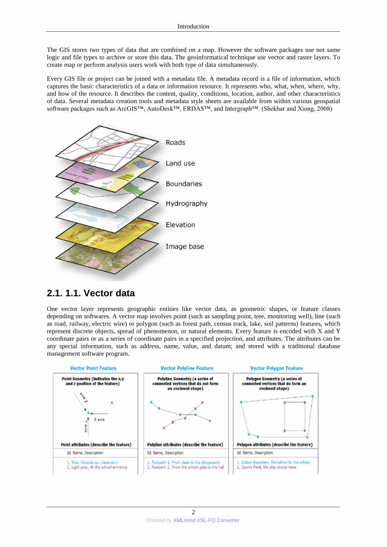
2.1. 1.1. Vector data
One vector layer represents geographic entities like vector data, as geometric shapes, or feature classes
depending on softwares. A vector map involves point (such as sampling point, tree, monitoring well), line (such
as road, railway, electric wire) or polygon (such as forest path, census track, lake, soil patterns) features, which
represent discrete objects, spread of phenomenon, or natural elements. Every feature is encoded with X and Y
coordinate pairs or as a series of coordinate pairs in a specified projection, and attributes. The attributes can be
any special information, such as address, name, value, and datum; and stored with a traditional database
management software program.
Introduction
3 Created by XMLmind XSL-FO Converter.
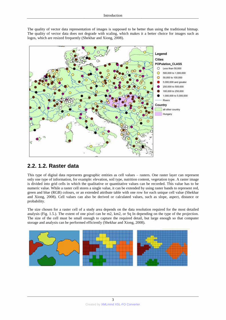
The quality of vector data representation of images is supposed to be better than using the traditional bitmap.
The quality of vector data does not degrade with scaling, which makes it a better choice for images such as
logos, which are resized frequently (Shekhar and Xiong, 2008).
2.2. 1.2. Raster data
This type of digital data represents geographic entities as cell values – rasters. One raster layer can represent
only one type of information, for example: elevation, soil type, nutrition content, vegetation type. A raster image
is divided into grid cells in which the qualitative or quantitative values can be recorded. This value has to be
numeric value. While a raster cell stores a single value, it can be extended by using raster bands to represent red,
green and blue (RGB) colours, or an extended attribute table with one row for each unique cell value (Shekhar
and Xiong, 2008). Cell values can also be derived or calculated values, such as slope, aspect, distance or
probability.
The size chosen for a raster cell of a study area depends on the data resolution required for the most detailed
analysis (Fig. 1.5.). The extent of one pixel can be m2, km2, or Sq In depending on the type of the projection.
The size of the cell must be small enough to capture the required detail, but large enough so that computer
storage and analysis can be performed efficiently (Shekhar and Xiong, 2008).

Introduction
4 Created by XMLmind XSL-FO Converter.
Raster layers represent continuously changing phenomenon over the space such as elevation, while the vector
layers illustrate only the significant discrete objects. Consequently, the raster images are predominantly analysis
oriented and suitable for evaluating environmental models. However vector layers are stored efficient and they
could produce simple thematic maps.
Introduction
5 Created by XMLmind XSL-FO Converter.
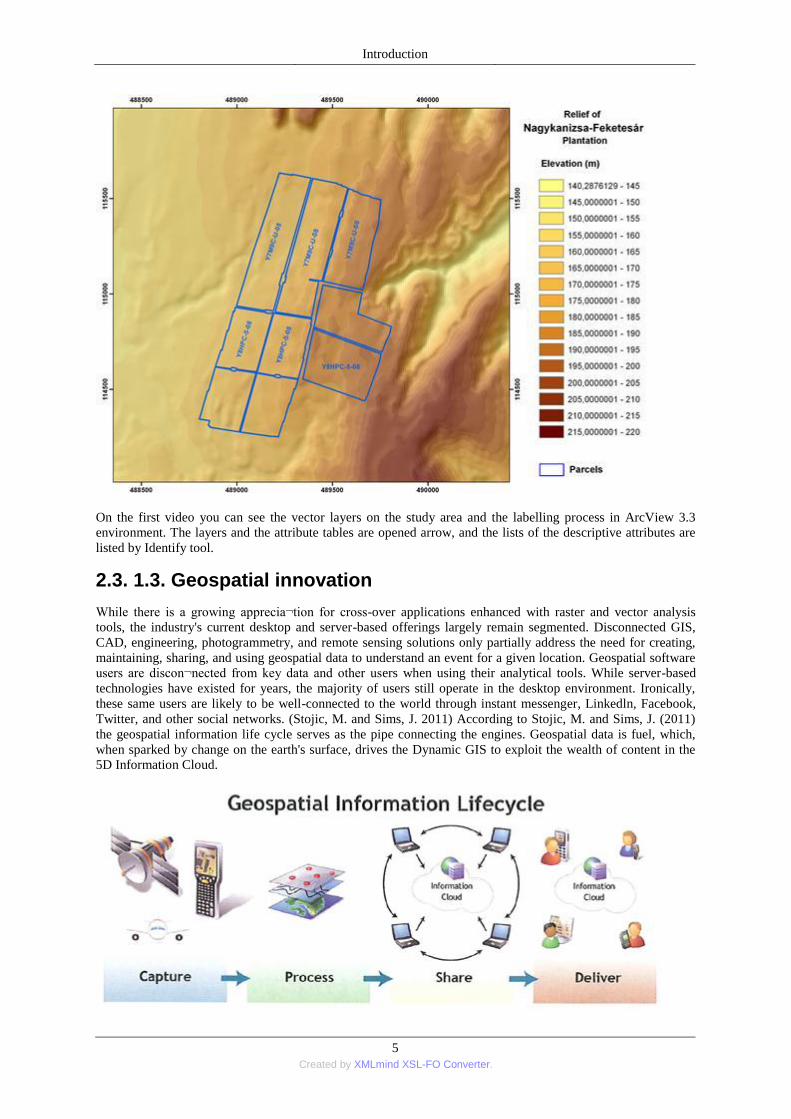
On the first video you can see the vector layers on the study area and the labelling process in ArcView 3.3
environment. The layers and the attribute tables are opened arrow, and the lists of the descriptive attributes are
listed by Identify tool.
2.3. 1.3. Geospatial innovation
While there is a growing apprecia¬tion for cross-over applications enhanced with raster and vector analysis
tools, the industry's current desktop and server-based offerings largely remain segmented. Disconnected GIS,
CAD, engineering, photogrammetry, and remote sensing solutions only partially address the need for creating,
maintaining, sharing, and using geospatial data to understand an event for a given location. Geospatial software
users are discon¬nected from key data and other users when using their analytical tools. While server-based
technologies have existed for years, the majority of users still operate in the desktop environment. Ironically,
these same users are likely to be well-connected to the world through instant messenger, Linkedln, Facebook,
Twitter, and other social networks. (Stojic, M. and Sims, J. 2011) According to Stojic, M. and Sims, J. (2011)
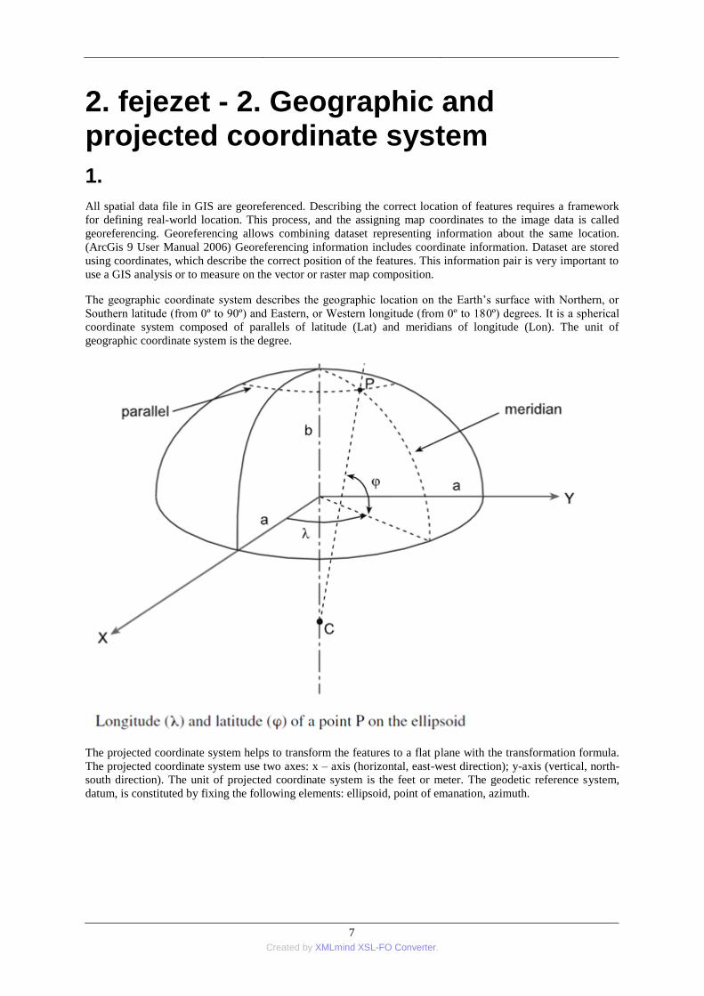
the geospatial information life cycle serves as the pipe connecting the engines. Geospatial data is fuel, which,
when sparked by change on the earth's surface, drives the Dynamic GIS to exploit the wealth of content in the
5D Information Cloud.

Introduction
6 Created by XMLmind XSL-FO Converter.
The four engines that power the lnformation Cloud are capture, process, share, and deliver. The geospatial
information life cycle serves as the pipe connecting the engines. Geospatial data is fuel, which, when sparked by
change on the earth's surface, drives the Dynamic GIS to exploit the wealth of content in the 5D Informa¬tion
Cloud.
The first engine includes airborne sensors (airborne digital imaging, LiDAR, UAV), satellites, and terrestrial
sensors (total station, GPS, video, terrestrial LiDAR, handheld devices). With all these sources feeding the
Information Cloud, the combined data and metadata are the fuel that is fed through the geospatial information
life cycle into the second engine for data fusion, processing, and production.
The second engine includes the geospatial processing tools for fusing and integrating geospatial source content
into software applications for the creation and update of geospatial data and informa¬tion products.
The third engine powering the Information Cloud is the ability to manage, fuse, and share geospatial data across
departments and regions, connecting to an organization's hub of geospatial data and information. With
increasing change, data volumes expand and the data captured and processed from a wide variety of "sensing"
sources creates a data management problem for finding and using geospatial data throughout an organization.
By effectively managing all sources of geospatial data (including GIS, CAD, surveying, remote sensing, and
photogrammetry), the value and usability of that data increases beyond departmental compartments and across
spatial domains to users who have a need to understand the changing earth.
The fourth engine for fully lever¬aging the Information Cloud enables the delivery of geospatial data AND
dynamic information products. This is done through on-demand geoprocessing over the Internet, to mobile
clients and the cloud through vertical market-focused SaaS implementations. The delivery engine leverages
stand-ards-based spatial data infrastructure (SDI) concepts, high-performance technologies, and geoprocessing
Web services for delivering geospatial information to Web portals, mobile clients, and a variety of thin- and
smart-client applications.
The Dynamic GIS catapults our entire industry into a new era, where integrated geospatial systems replace the
traditional domains of GIS, remote sensing, photo¬grammetry, surveying, and mapping. (Stojic, M. and Sims, J.
2011)
7 Created by XMLmind XSL-FO Converter.
2. fejezet - 2. Geographic and projected coordinate system
1.
All spatial data file in GIS are georeferenced. Describing the correct location of features requires a framework
for defining real-world location. This process, and the assigning map coordinates to the image data is called
georeferencing. Georeferencing allows combining dataset representing information about the same location.
(ArcGis 9 User Manual 2006) Georeferencing information includes coordinate information. Dataset are stored
using coordinates, which describe the correct position of the features. This information pair is very important to
use a GIS analysis or to measure on the vector or raster map composition.
The geographic coordinate system describes the geographic location on the Earth‘s surface with Northern, or
Southern latitude (from 0º to 90º) and Eastern, or Western longitude (from 0º to 180º) degrees. It is a spherical
coordinate system composed of parallels of latitude (Lat) and meridians of longitude (Lon). The unit of
geographic coordinate system is the degree.
The projected coordinate system helps to transform the features to a flat plane with the transformation formula.
The projected coordinate system use two axes: x – axis (horizontal, east-west direction); y-axis (vertical, north-
south direction). The unit of projected coordinate system is the feet or meter. The geodetic reference system,
datum, is constituted by fixing the following elements: ellipsoid, point of emanation, azimuth.
2. Geographic and projected
coordinate system
8 Created by XMLmind XSL-FO Converter.
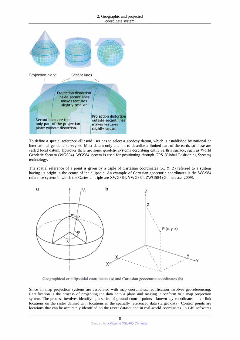
To define a special reference ellipsoid user has to select a geodesy datum, which is established by national or
international geodetic surveyors. Most datum only attempt to describe a limited part of the earth, so these are
called local datum. However there are some geodetic systems describing entire earth‘s surface, such as World
Geodetic System (WGS84). WGS84 system is used for positioning through GPS (Global Positioning System)
technology.
The spatial reference of a point is given by a triple of Cartesian coordinates (X, Y, Z) referred to a system
having its origin in the centre of the ellipsoid. An example of Cartesian geocentric coordinates is the WGS84
reference system in which the Cartesian triple are XWGS84, YWGS84, ZWGS84 (Gomarasca, 2009).
Since all map projection systems are associated with map coordinates, rectification involves georeferencing.
Rectification is the process of projecting the data onto a plane and making it conform to a map projection
system. The process involves identifying a series of ground control points—known x,y coordinates—that link
locations on the raster dataset with locations in the spatially referenced data (target data). Control points are
locations that can be accurately identified on the raster dataset and in real-world coordinates. In GIS softwares
2. Geographic and projected
coordinate system
9 Created by XMLmind XSL-FO Converter.
the list of the supported map projections is different, but every program packages process many standard
coordinate systems and numerous local system. The ArcGIS versions support the Hungarian coordinate system
(EOV) so called HD1972 Egységes Országos Vetület. As well as user can also create a custom coordinate
system with describing the projection file.
1.1. Practice 1: Define coordinate system in ArcGIS
1.1.1. Exercise 1.1.
If the input dataset or vector layers, created by GPS survey or rectified in any software ambient, possess any
associated projection parameters, but the coordinate system has not defined in ArcGIS first the projection file
has to be defined before any analysis.
1.Start ArcMap, with a new, empty map, and add the data downloaded from GPS with parameters of the known
coordinate system. The data must not have a defined coordinate system.
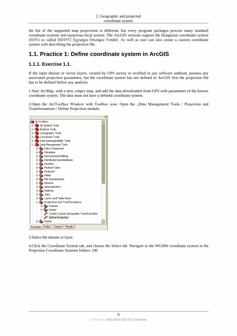
2.Open the ArcToolbox Window with Toolbox icon. Open the „Data Management Tools / Projection and
Transformations / Define Projection module.
3.Select the dataset or layer.
4.Click the Coordinate System tab, and choose the Select tab. Navigate to the WGS84 coordinate system in the
Projection Coordinate Systems folders. OK

2. Geographic and projected
coordinate system
10 Created by XMLmind XSL-FO Converter.
To assign the coordinate system, ―import‖ button can be useable, if there is any layer with required coordinate
system in the database. To create new custom coordinate system ―new‖ button has to be used.
When the coordinate system is defined, the other data, which add to the ArcMap session, is fitting into the
current coordinate system.
5. Add a new data layer with other coordinate system to the map composition.
One dialog box appears to show which geodetic datum of map layers differ from the other maps.
6. Press the ―Transformation‖ button. Select the coordinate system of the added layer, then the coordinate
system of the data frame. Select the useable transformation methods. OK.
The original coordinate system of the added layer is unchanged, this operation means only displaying.
1.1.2. Exercise 1.2.

2. Geographic and projected
coordinate system
11 Created by XMLmind XSL-FO Converter.
The geodetic datum of the layer can be defined in ArcCatalog. In the catalogue tree, navigate and select the
layer.
Right-click on the layer name and click Properties. On the Properties dialog box, assign coordinate system
according to previous method.
If you need to change the coordinate system of any layer to a different one, Project (feature layer) or Project
Raster (raster layer) tools has to be used.
7. Open Data management Tools / Projection and Transformation / Feature / Project tool – in the case of vector
layer; or Data management Tools / Projection and Transformation / Raster / Project raster tool – in the case of
raster layer.
8. Enter the input and output layer name.
9. Select the required coordinate system.
10. Select the transformation method. OK.

2. Geographic and projected
coordinate system
12 Created by XMLmind XSL-FO Converter.
1.2. Practice 2: Rectify an image map to EOV coordinate system in ArcGIS
This process involves identifying a series of ground control points (GCPs) with known the real location - x,y
coordinates. There are many different types of GCPs that can be used to identify locations, such as road or
stream intersections, street corners, or the corners of the buildings. The control points are used to convert the
raster dataset to the spatially correct location. The connection between one control point on the raster dataset
and the corresponding control point on the aligned target data is a link. The number of links depends on the
transformation method to project the raster dataset to map coordinates.
Conflation technologies are applied in many application domains using high quality spatial data such as GIS. In
general, the goal of conflation is to combine the best quality elements of both datasets to overlay different
dataset with each other. Based on the types of geospatial datasets dealt with, the conflation technologies can be
categorized into the following three groups: Vector to vector data conflation; Vector to raster data conflation;
Raster to raster data conflation. The most important step of the conflation is to find a set of conjugate point
pairs, termed control point pairs, in two datasets. (Shekhar and Xiong, 2008)

2. Geographic and projected
coordinate system
13 Created by XMLmind XSL-FO Converter.
These exercises were worked out for practical purposes used by ArcGIS® 9 Using ArcGIS Desktop.
1.2.1. Exercise 2.1.
Conflation method with ArcGis software
1. In ArcMap, display the layers having map coordinates.
2. Add the raster dataset that you want to georeference.
3. Open the Georeferencing toolbar under View menu, point to Toolbars, and click Georeferencing
4. In the table of contents, right-click the referenced dataset and click Zoom to Layer.
5. From the Georeferencing toolbar, click the Layer drop-down arrow and click the target raster layer that you
want to georeference.
6. Click Georeferencing and click Fit To Display.

2. Geographic and projected
coordinate system
14 Created by XMLmind XSL-FO Converter.
7. The target layer will display with the raster dataset in the same area. If both layers are raster images, the target
layer has to be transparent. Open the Effects toolbar under View menu, point to Toolbars, and click Effects.
8. Click the Layer drop-down arrow, select the target raster layer and use the Adjust transparency icon to change
the visibility of the layer.
9. Look for GCPs such as road intersections, land features, building corners or other objects that you can
identify and match in your raster dataset and aligned datasets. Before placement of the GCPs, switch off the
Auto adjust tool under the Georeferencing menu in order to prevent the target raster from becoming deformed.
Consequently the link will be visible (blue line).
10. Click the Add Control Points tool to add control points. To add a link, click the mouse pointer on:
1. the target raster data to place on control point
2. the raster dataset with coordinate system to place on the associated control point

2. Geographic and projected
coordinate system
15 Created by XMLmind XSL-FO Converter.
11. Add enough links for the type of transformation. You need a minimum of three links for a spline or 1st-order
polynomial (affine), six links for a 2nd-order polynomial, and ten links for an affine or 3rd-order polynomial.
12. Click View Link Table to evaluate the transformation. Select the transformation method from drop-down list
and examine the residual error for each link and total RMS error. All error values are expressed in term of the
root mean square error (RMSE), it is an estimator of general model performance - precision (Zeilhofer et al.,
2011). The (RMS) average value of each residual gradient grid is calculated in order to give an estimate of the
error in the numerical gradient values at each cell size (Jones K. H., 1998).
You can delete an unwanted link from the Link Table dialog box. After deleting incorrect GCP, use Auto adjust
to verify the changes.
13. If you‘re satisfied with the registration, click Georeferencing menu and select Update Georeferencing to
save the transformation information with the raster dataset. This creates a new file with the same name as the
raster dataset but with an .aux.xml file extension.
14. You can permanently transform your raster dataset after georeferencing by using the Rectify command;
click Georeferencing and click Rectify
This exercise was worked out for practical purposes used by ArcGIS® 9 Using ArcGIS Desktop.

2. Geographic and projected
coordinate system
16 Created by XMLmind XSL-FO Converter.
1.2.2. Exercise 2.2.
Conflation method with ERDAS software
The above mentioned process can be performed in other software environment also; however there are some
differences from the method in ArcGis. In this exercise, you rectify a previous soil map using a georeferenced
topographic map of the same area. The topographic map is rectified to the Hungarian coordinate system – EOV
projection, however this projection is not defined in Erdas.
1. Start the Erdas Imagine software.
2. Click the Viewer icon on the ERDAS IMAGINE icon panel to open two Classic Viewer windows. Then
select the target raster layer in the first viewer and the referenced raster in the second viewer. The Erdas
software works with numerous raster file format as compared with the ArcGis.
The first difference is the display, since the images is opened in two independent windows. When the
topographical map is opened, the coordinate values are shown in the status bar.
3. Start the Raster menu / Geometric Correction Tool from the first Viewer (the Viewer displaying the file to be
rectified).
2. Geographic and projected
coordinate system
17 Created by XMLmind XSL-FO Converter.
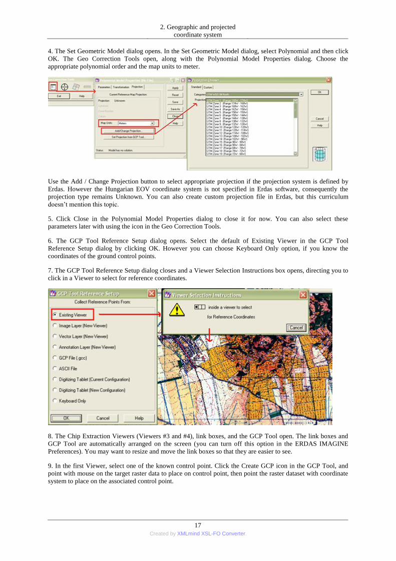
4. The Set Geometric Model dialog opens. In the Set Geometric Model dialog, select Polynomial and then click
OK. The Geo Correction Tools open, along with the Polynomial Model Properties dialog. Choose the
appropriate polynomial order and the map units to meter.
Use the Add / Change Projection button to select appropriate projection if the projection system is defined by
Erdas. However the Hungarian EOV coordinate system is not specified in Erdas software, consequently the
projection type remains Unknown. You can also create custom projection file in Erdas, but this curriculum
doesn‘t mention this topic.
5. Click Close in the Polynomial Model Properties dialog to close it for now. You can also select these
parameters later with using the icon in the Geo Correction Tools.
6. The GCP Tool Reference Setup dialog opens. Select the default of Existing Viewer in the GCP Tool
Reference Setup dialog by clicking OK. However you can choose Keyboard Only option, if you know the
coordinates of the ground control points.
7. The GCP Tool Reference Setup dialog closes and a Viewer Selection Instructions box opens, directing you to
click in a Viewer to select for reference coordinates.
8. The Chip Extraction Viewers (Viewers #3 and #4), link boxes, and the GCP Tool open. The link boxes and
GCP Tool are automatically arranged on the screen (you can turn off this option in the ERDAS IMAGINE
Preferences). You may want to resize and move the link boxes so that they are easier to see.
9. In the first Viewer, select one of the known control point. Click the Create GCP icon in the GCP Tool, and
point with mouse on the target raster data to place on control point, then point the raster dataset with coordinate
system to place on the associated control point.

2. Geographic and projected
coordinate system
18 Created by XMLmind XSL-FO Converter.
In order to see easier the GCPs you can change the colour under the Color columns with left click. Digitize at
least two more GCPs pairs in each Viewer by repeating the above steps. The GCPs you digitize should be
spread out across the image to form a large triangle. After you digitize the fourth GCP in the first Viewer, note
that the GCP is automatically matched in the second Viewer, if the Toggle Fully Automatic GCP Editor icon is
on.
10. Examine the residual values and the total RMS error. Select to incorrect GCPs and move to the correct place
with the help of the small viewers 3-4, or delete it. To delete a GCP, select the GCP in the Cell Array in the
GCP Tool and then right-hold in the Point # column to select Delete Selection.
11. Click the Resample icon in the Geo Correction Tools. The Resample dialog opens. Resampling is the
process of calculating the file values for the rectified image and creating the new file. All of the raster data
layers in the source file are resampled. The output image has as many layers as the input image. ERDAS
IMAGINE provides these widely-known resampling algorithms: Nearest Neighbour, Bilinear Interpolation,
Cubic Convolution, and Bicubic Spline.
12. Enter file name for the new georeferenced image file. Under Resample Method, click the dropdown list and
select the appropriate method. Click OK in the Resample dialog to start the resampling process. Click OK in the
Job Status dialog when the job is 100% complete.
This exercise was worked out for practical purposes used by ERDAS IMAGINE ® Tour Guides™.
19 Created by XMLmind XSL-FO Converter.
3. fejezet - 3. Surface modelling
1.
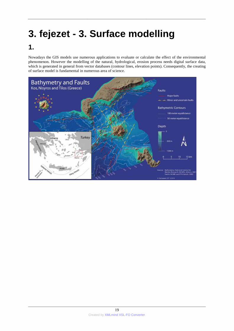
Nowadays the GIS models use numerous applications to evaluate or calculate the effect of the environmental
phenomenon. However the modelling of the natural, hydrological, erosion process needs digital surface data,
which is generated in general from vector databases (contour lines, elevation points). Consequently, the creating
of surface model is fundamental in numerous area of science.

3. Surface modelling
20 Created by XMLmind XSL-FO Converter.
The most spectacular application of the DEMs is the representations of volcanoes, hilly or coastal region.
Geographers and geologists have developed or integrated various spatial data analysis for managing and
analyzing multi-disciplinary, lithology, volcanological information or the data-sets of the anthropogenic
structures (Gogu et al. 2006; Fornaciai et al., 2010; De Rienzo et al. 2008).

3. Surface modelling
21 Created by XMLmind XSL-FO Converter.
DEM creation is also very important in area of the agriculture and the soils science. Casalí et al. (2009)
determined the long-term erosion rates, and the remained soil surface level in vineyards with the help of the
DEMs.
Furthermore, Katsianis et al., (2008) represent a formal data model and complete digital workflow in 3D using
the prehistoric site in Greece, as a case study. They chosen Esri‘s ArcGIS as the unifying software platform for
several key reasons: being an industry standard, incorporating a functional 3D viewing environment (ArcScene),
presenting abilities for customization, having a spatial database system with object-oriented characteristics and
supporting communication with external programs (Rock-Ware, EVS, CAD, Sketch Up).
The monitoring and modelling of the gully erosion was examined by Marzolff and Poesen (2009) with using a
hybrid method combining stereo matching for mass-point extraction with manual 3D editing and digitizing,
high-resolution DEMs.
The digital surface model is a representation of features, either real or hypothetical, in three-dimensional space.
In the last decades researchers have investigated a variety of technical issues related to 3D data processing,
visualization, data management and spatial analysis in order to represent the world more or less closely to
reality. A 3D surface is usually derived, or calculated, using specially designed algorithms that sample point,
line or polygon data and convert them into a digital 3D surface (http://webhelp.esri.com). GIS softwares can
create and store different types of surface model: TIN, raster, terrain and voxel based.
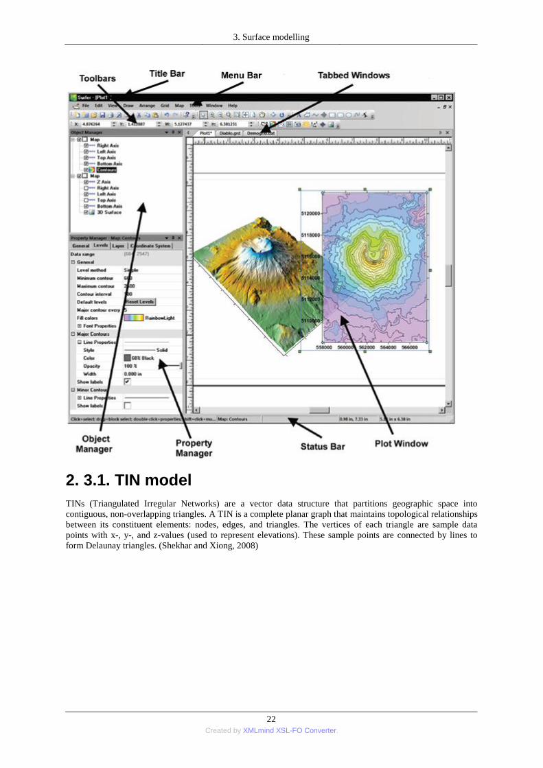
Surfer is a grid-based mapping program that interpolates irregularly spaced XYZ data into a regularly spaced
grid. The grid is used to produce different types of maps including contour, vector, image, shaded relief, 3D
surface, and 3D wireframe maps. (http://www.goldensoftware.com)
3. Surface modelling
22 Created by XMLmind XSL-FO Converter.
2. 3.1. TIN model
TINs (Triangulated Irregular Networks) are a vector data structure that partitions geographic space into
contiguous, non-overlapping triangles. A TIN is a complete planar graph that maintains topological relationships
between its constituent elements: nodes, edges, and triangles. The vertices of each triangle are sample data
points with x-, y-, and z-values (used to represent elevations). These sample points are connected by lines to
form Delaunay triangles. (Shekhar and Xiong, 2008)
3. Surface modelling
23 Created by XMLmind XSL-FO Converter.
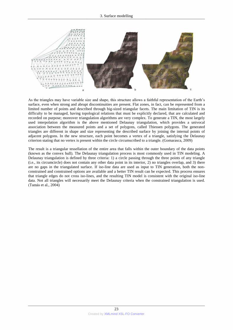
As the triangles may have variable size and shape, this structure allows a faithful representation of the Earth‘s
surface, even when strong and abrupt discontinuities are present. Flat zones, in fact, can be represented from a
limited number of points and described through big-sized triangular facets. The main limitation of TIN is its
difficulty to be managed, having topological relations that must be explicitly declared, that are calculated and
recorded on purpose; moreover triangulation algorithms are very complex. To generate a TIN, the most largely
used interpolation algorithm is the above mentioned Delaunay triangulation, which provides a univocal
association between the measured points and a set of polygons, called Thiessen polygons. The generated
triangles are different in shape and size representing the described surface by joining the internal points of
adjacent polygons. In the new structure, each point becomes a vertex of a triangle, satisfying the Delaunay
criterion stating that no vertex is present within the circle circumscribed to a triangle. (Gomarasca, 2009)
The result is a triangular tessellation of the entire area that falls within the outer boundary of the data points
(known as the convex hull). The Delaunay triangulation process is most commonly used in TIN modeling. A
Delaunay triangulation is defined by three criteria: 1) a circle passing through the three points of any triangle
(i.e., its circumcircle) does not contain any other data point in its interior, 2) no triangles overlap, and 3) there
are no gaps in the triangulated surface. If iso-line data are used as input to TIN generation, both the non-
constrained and constrained options are available and a better TIN result can be expected. This process ensures
that triangle edges do not cross iso-lines, and the resulting TIN model is consistent with the original iso-line
data. Not all triangles will necessarily meet the Delaunay criteria when the constrained triangulation is used.
(Tamás et al., 2004)
3. Surface modelling
24 Created by XMLmind XSL-FO Converter.
3. 3.2. DEM – DTM - DSM
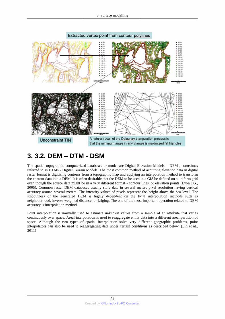
The spatial topographic computerized databases or model are Digital Elevation Models – DEMs, sometimes
referred to as DTMs - Digital Terrain Models. The most common method of acquiring elevation data in digital
raster format is digitizing contours from a topographic map and applying an interpolation method to transform
the contour data into a DEM. It is often desirable that the DEM to be used in a GIS be defined on a uniform grid
even though the source data might be in a very different format - contour lines, or elevation points (Lyon J.G.,
2005). Common raster DEM databases usually store data in several meters pixel resolution having vertical
accuracy around several meters. The intensity values of pixels represent the height above the sea level. The
smoothness of the generated DEM is highly dependent on the local interpolation methods such as
neighbourhood, inverse weighted distance, or kriging. The one of the most important operation related to DEM
accuracy is interpolation method.
Point interpolation is normally used to estimate unknown values from a sample of an attribute that varies
continuously over space. Areal interpolation is used to reaggregate entity data into a different areal partition of
space. Although the two types of spatial interpolation solve very different geographic problems, point
interpolators can also be used to reaggregating data under certain conditions as described below. (Lin et al.,
2011)

3. Surface modelling
25 Created by XMLmind XSL-FO Converter.
Digital Terrain Models (DTMs) are getting more and more important in geographical data processing and
analysis: they allow modelling, analysis and visualization of phenomena related to the territory morphology (or
to any other characteristic of the territory different from elevation) (Gomarasca, 2009). There is one more
definition related to surface model, the Digital Surface Models (DSM). DSM describes the terrestrial surface,
including the objects covering it like buildings, vegetation and in general describes it through known geometric
primitives (rectangles or triangles). 3D geoinformation research is often related to the representation of the built
or mane-made environment (Kjems et al, 2009).

3. Surface modelling
26 Created by XMLmind XSL-FO Converter.
4. 3.3. New technologies in surface modeling
A terrain dataset is a TIN-based data structure with multiple levels of resolution. Terrains include pyramids that
provide the appropriate levels of detail for use at multiple scales. A terrain dataset is built from multiple data
sources such as LIDAR mass point collections, 3D break lines, and 3D-based survey observations. The data
sources used to create terrain datasets are managed as a set of integrated feature classes in the geodatabase.
(http://webhelp.esri.com)
The laser technology is now available for photogrammetric. The technology is a still developing and continuous
representation method of the Earth‘s surface. It produces a huge amount of data to be processed, visualized and
integrated into the photogrammetric process.
Laser scanning is a surveying technology for rapid and detailed acquisition of a surface in terms of a set of
points on that surface, a so-called point cloud. Laser scanners are operated from airborne platforms as well as
from terrestrial platforms (usually tripods). The time elapsed between emitting and receiving a pulse is
multiplied by the speed of light to derive the distance between the laser range finder and the reflecting object.
This distance is combined with position and attitude information of the airborne platform, as well as the pointing
direction of the laser beam, to calculate the location of the reflecting object. (Shekhar and Xiong, 2008)

3. Surface modelling
27 Created by XMLmind XSL-FO Converter.
During last years the LIDAR (Light Detection And Ranging) has been used as a very good option to terrestrial
surface surveying. In recent years, LIDAR sensors have been widely used to measure environmental parameters
such as the structural characteristics of surface, features, or forests. This new data acquisition technology is now
capable of collecting data in a much denser and more precise manner. For example, LiDAR technology, which
have dispersal and irregular data structure, can acquire up to 16 points per 1m2 with position accuracy around
0.1m (Dalyot and Doytsher, 2009). It can survey 3D positions over the terrestrial surface at speed beyond
comparison to the Topography or Photogrammetry (De Lara et al., 2009).
3. Surface modelling
28 Created by XMLmind XSL-FO Converter.
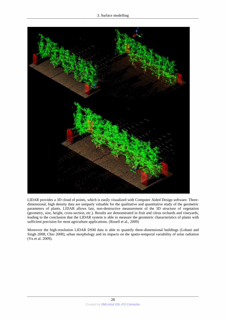
LIDAR provides a 3D cloud of points, which is easily visualized with Computer Aided Design software. Three-
dimensional, high density data are uniquely valuable for the qualitative and quantitative study of the geometric
parameters of plants. LIDAR allows fast, non-destructive measurement of the 3D structure of vegetation
(geometry, size, height, cross-section, etc.). Results are demonstrated in fruit and citrus orchards and vineyards,
leading to the conclusion that the LIDAR system is able to measure the geometric characteristics of plants with
sufficient precision for most agriculture applications. (Rosell et al., 2009)
Moreover the high-resolution LIDAR DSM data is able to quantify three-dimensional buildings (Lohani and
Singh 2008; Chio 2008), urban morphology and its impacts on the spatio-temporal variability of solar radiation
(Yu et al. 2009).

3. Surface modelling
29 Created by XMLmind XSL-FO Converter.
Many researchers propose 3D grid representation (voxels) as the most appropriate data format to visualize
continuous phenomena in true 3D format. A voxel (volumetric pixel or Volumetric Picture Element) is a volume
element, representing a value on a regular grid in real three dimensional space. (De Rienzo et al., 2008;
Kirkpatrick and Weishampel, 2005; Dong, 2009)
5. 3.4. Surface or spatial analysis tools

3. Surface modelling
30 Created by XMLmind XSL-FO Converter.
The surface model of the topographic surface can be used to characterizing geomorphological features over the
different applications, such as slope, aspect, length of the slope, curvature, perspective views, view shed
analysis, height profiles and volume calculations. This family of tools is generally calculated from the finest
spatial scale database.
Slope maps are also raster datasets where the cell value represents the angle between the horizontal and the local
gradient of the DEM. There are special classes of slopes depending on the different area of science.
The cell values of aspect maps represent the angle (azimuth) between the north direction and the local gradient
(planar components). Usually nine classes are considered: one referred to the null value (flat areas), the other
height to the main direction sectors (north, northeast, east, south-east, south, south-west, west, north-west).

3. Surface modelling
31 Created by XMLmind XSL-FO Converter.
The Hillshade tool creates a shaded relief raster from a raster. The illumination source is considered at infinity.
The hillshade raster has an integer value range of 0 to 255.
Performs visibility analysis on a raster by determining how many observation points can be seen from each cell
location of the input raster or which cell locations can be seen by each observation point. The visibility of each
cell centre is determined by comparing the altitude angle to the cell centre with the altitude angle to the local
horizon. The local horizon is computed by considering the intervening terrain between the point of observation
and the current cell centre. If the point lies above the local horizon, it is considered visible.
(http://webhelp.esri.com)
5.1. Practice 3: Create digital surface models from vector data
5.1.1. Exercise 3.1. Create TIN surface features in ArcGIS
1.Start ArcMap, with a new, empty map
2.Open the input vector layers (contour or elevation point). The data must have a defined coordinate system (see
above) with X and Y coordinates, and Z – elevation values. Height (Z) Field is the name of the attribute to be
used for height information.

3. Surface modelling
32 Created by XMLmind XSL-FO Converter.
3.Under the Tools menu / Extensions, select the 3D Analyst option.
4.First one TIN must be defined using the Create Tin function. Open the ArcToolbox Window with icon. Select
the 3D Analyst toolbox / TIN Creation tools / Create TIN tool. Enter the output file name and its path.
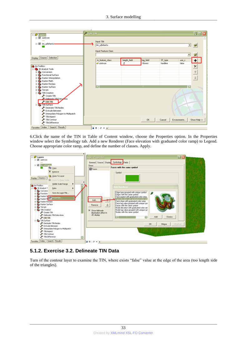
5.Select the 3D Analyst toolbox / TIN Creation tools / Edit TIN tool. Select the input TIN. Add features to the
existing TIN. Multiple feature layers can be added at the same time with the + icon. From the drop-down list
select the height field - Z. OK.
3. Surface modelling
33 Created by XMLmind XSL-FO Converter.
6.Click the name of the TIN in Table of Content window, choose the Properties option. In the Properties
window select the Symbology tab. Add a new Renderer (Face elevation with graduated color ramp) to Legend.
Choose appropriate color ramp, and define the number of classes. Apply.
5.1.2. Exercise 3.2. Delineate TIN Data
Turn of the contour layer to examine the TIN, where exists ―false‖ value at the edge of the area (too length side
of the triangles).

3. Surface modelling
34 Created by XMLmind XSL-FO Converter.
7.Select the 3D Analyst toolbox / TIN Creation tools / Delineate TIN Data Area tool to define the data area, or
interpolation zone, of a TIN based on triangle edge length. Define the value of the Maximum Edge Length.
8. Turn on the input vector layer to examine the result.
3. Surface modelling
35 Created by XMLmind XSL-FO Converter.
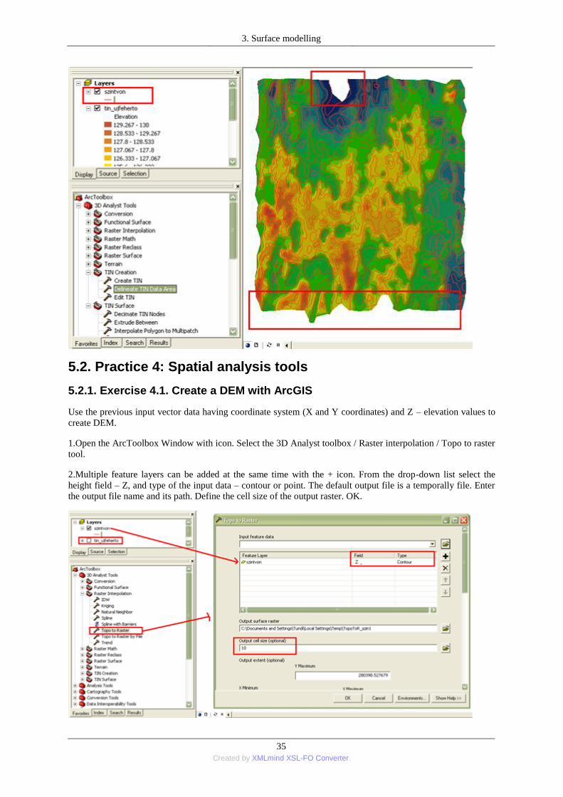
5.2. Practice 4: Spatial analysis tools
5.2.1. Exercise 4.1. Create a DEM with ArcGIS
Use the previous input vector data having coordinate system (X and Y coordinates) and Z – elevation values to
create DEM.
1.Open the ArcToolbox Window with icon. Select the 3D Analyst toolbox / Raster interpolation / Topo to raster
tool.
2.Multiple feature layers can be added at the same time with the + icon. From the drop-down list select the
height field – Z, and type of the input data – contour or point. The default output file is a temporally file. Enter
the output file name and its path. Define the cell size of the output raster. OK.
3. Surface modelling
36 Created by XMLmind XSL-FO Converter.
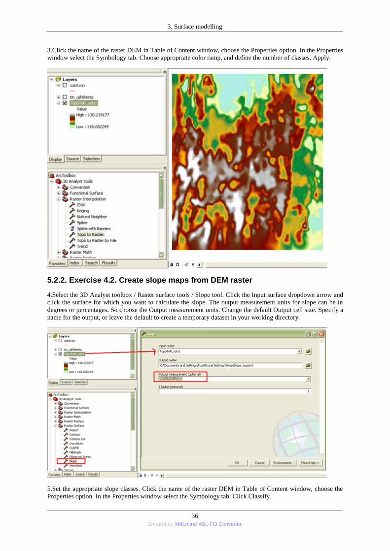
3.Click the name of the raster DEM in Table of Content window, choose the Properties option. In the Properties
window select the Symbology tab. Choose appropriate color ramp, and define the number of classes. Apply.
5.2.2. Exercise 4.2. Create slope maps from DEM raster
4.Select the 3D Analyst toolbox / Raster surface tools / Slope tool. Click the Input surface dropdown arrow and
click the surface for which you want to calculate the slope. The output measurement units for slope can be in
degrees or percentages. So choose the Output measurement units. Change the default Output cell size. Specify a
name for the output, or leave the default to create a temporary dataset in your working directory.
5.Set the appropriate slope classes. Click the name of the raster DEM in Table of Content window, choose the
Properties option. In the Properties window select the Symbology tab. Click Classify.

3. Surface modelling
37 Created by XMLmind XSL-FO Converter.
6. Click the Method drop-down arrow and click the classification method you want to use. Click the Classes
drop-down arrow and click the number of classes you want to display. Type a new upper value of the range on
the basis of histogram or specific intervals. OK. Enter Label for every class. OK.
5.2.3. Exercise 4.3. Display 3D view
7.Start the ArcScene from the ArcMap with the icon. Add the raster layers – DEM, slope - to Table of Content.
8.First set the base height of DEM. Double click on the layer name. Click the Base Height tab. Select and enter
the name and path of the DEM. Set the z-unit conversion to 10, if the sample area is lowland. Examine the
result.
9.Perform the previous step on the drapping layer – slope at the same way. Select and enter the name and path of
the DEM. Select the Symbology tab. Choose color ramp. Select the Use Hillshade Effect option. OK.

3. Surface modelling
38 Created by XMLmind XSL-FO Converter.
10.Open the Effects toolbar under View menu, point to Toolbars, and click 3D Effects.
11.Click the Layer drop-down arrow; select the target raster layer – slope, and use the Adjust transparency icon
to change the visibility of the layer.
These exercises were worked out for practical purposes used by ESRI Desktop Online Help.

39 Created by XMLmind XSL-FO Converter.
4. fejezet - 4. Remote sensing
1.
Aerial photography and satellite imagery, both photographic and telemetric, recorded at various wavelengths or
bands of the electromagnetic spectrum are included in these tools (Pavlopoulos et al., 2009). From classical
geography, scientific activities in Earth Observation have undergone a rapid expansion, and more and more
economic sectors tend to employ territorial data acquired by ground survey, global satellite positioning systems,
traditional and digital photogrammetry, multi- and hyperspectral remote sensing from airplane and satellite, with
images both passive optical and active microwave (radar) at different geometric, spectral, radiometric and
temporal resolutions, although there is still only limited awareness of how to use all the available potential
correctly.
The first photographs of the Earth taken from space were released in the early 1960s. In 1972 the U.S.A.
launched its first Earth Resources Technology Satellite ERTS-1, which was later renamed LANDSAT-1.
(Cracknell and Hayes, 1993)
The resulting data and information are represented in digital and numerical layers managed in Geographical
Information Systems and Decision Support Systems, often based on the development of Expert Systems.
(Gomarasca, 2009) Remote sensing is the science and art of obtaining information about the properties of
electromagnetic waves emitted, reflected or diffracted without touching the object (Campbell, 2002). Remote
sensing enables a unique perspective to map and monitor on large areas because it measures emitted or reflected
energy at wavelengths with a wider range than human vision.
Remote sensing includes techniques to derive information from a site at a known distance from the sensor.
Imaging data are either gathered as photographs and optically digitized, or are measured directly using a digital
instrument on a remote sensing satellite or aircraft. Every element on the Earth reflects, absorbs and transmits
part of an incident radiation to different percentages according to its structural, chemical and chromatic
qualities.
Radar or satellite data can be used in GIS applications for numerous science areas: geology, archaeology,
vegetation classification, crop monitoring, glaciology, oceanography, soil science, hydrology or pollution
monitoring.

4. Remote sensing
40 Created by XMLmind XSL-FO Converter.
The one of most important parameters, which characterized the instruments, are the wavelength (or frequency),
the amplitude, and the direction of the surveying. Electromagnetic radiance is the information reaching a sensor
from the objects located on the Earth. For example, the problem with most widely used multispectral systems is
that they only have a limited number of bands with each covering a very wide region in the spectrum (>
100nm); and within such a wide spectral region a lot of subtle information is averaged, generalized or even
concealed. (Zhou, 2007).

4. Remote sensing
41 Created by XMLmind XSL-FO Converter.
Every Earth‘s surface (soil-, rock-, vegetation-, water-, and building surface) and the variations of these have a
unique spectral profile. However these unique spectral features of the surface varieties or vegetation species,
such as reflectance peaks or absorption troughs in the spectrum, are often lost in broad-band spectral reflectance.
2. 4.1. Sensors
Change detection or monitoring methodology can be greatly facilitated by the use of digital imaging data from
sensors. (Lyon J.G., 2005) Imaging data have the capabilities to supply spatial and spectral data over large areas,
4. Remote sensing
42 Created by XMLmind XSL-FO Converter.
and to do so at a potentially lower relative cost than fieldwork and mapping alone. In remote sensing, there are
two typologies of instruments, passive and active, based on the source of incident radiation on the Earth‘s
surface and on wavelength intervals. In passive remote sensing, sensors operate in wavelength intervals from
ultraviolet to thermal infrared; in active systems such as radar, they operate in microwave intervals. In passive
remote sensing, the source of information is scattered and/or absorbed solar and emitted thermal radiation,
which allows us to study and characterize objects through their spectrally variable response. (Gomarasca, 2009)
A passive system is restricted to radiation that is emitted from the surface of the Earth or which is present in
reasonable quantity in the radiation that is emitted by the Sun and then reflected from the surface of the Earth.
An active instrument is restricted to wavelength ranges in which reasonable intensities of the radiation can be
generated by the remote sensing instrument on the platform on which it is operating. Active sensors operating in
the visible and infrared parts of the spectrum, while not being flown on satellites, are flown on aircraft.
(Cracknell and Hayes, 1993)
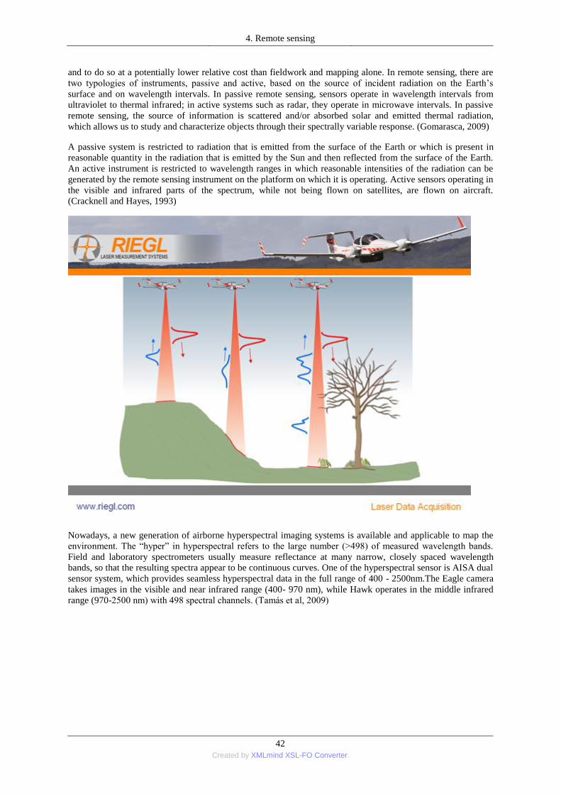
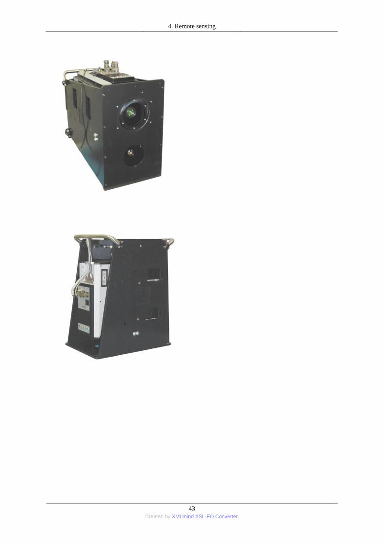
Nowadays, a new generation of airborne hyperspectral imaging systems is available and applicable to map the
environment. The ―hyper‖ in hyperspectral refers to the large number (>498) of measured wavelength bands.
Field and laboratory spectrometers usually measure reflectance at many narrow, closely spaced wavelength
bands, so that the resulting spectra appear to be continuous curves. One of the hyperspectral sensor is AISA dual
sensor system, which provides seamless hyperspectral data in the full range of 400 - 2500nm.The Eagle camera
takes images in the visible and near infrared range (400- 970 nm), while Hawk operates in the middle infrared
range (970-2500 nm) with 498 spectral channels. (Tamás et al, 2009)
4. Remote sensing
43 Created by XMLmind XSL-FO Converter.

4. Remote sensing
44 Created by XMLmind XSL-FO Converter.
3. 4.2. Multispectral

4. Remote sensing
45 Created by XMLmind XSL-FO Converter.
The multispectral image can be used as a photo or a scientific basic database to subject to differences photo
interpretation methods.
The Multispectral Scanner System (MSS) sensors were line scanning devices observing the Earth perpendicular
to the orbital track. The cross-track scanning was accomplished by an oscillating mirror; six lines were scanned
simultaneously in each of the four spectral bands for each mirror sweep. The forward motion of the satellite
provided the along-track scan line progression. The first five Landsat carried the MSS sensor which responded
to Earth-reflected sunlight in four spectral bands. Landsat 3 carried an MSS sensor with an additional band,
designated band 8, that responded to thermal (heat) infrared radiation. Four years after the launch of the first
Landsat satellite (then called the Earth Resources Technology Satellite, ERTS-1), a U.S. Geological Survey
Professional Paper entitled, "ERTS-1 A New Window on Our Planet" was published. The publication
documented how visual examination of images from a space-based vantage point could benefit disciplines such
as geology, hydrology, forestry, geography, cartography, agriculture, land use planning and rangeland
management. Landsat data have helped to improve our understanding of Earth. Thanks to Landsat, today we
have a better understanding of things as diverse as coral reefs, tropical deforestation, and Antarctica's glaciers.
The 30 m spatial resolution and 185 km swath of Landsat imagery fills an important scientific niche because the
orbit swaths are wide enough for global coverage every season of the year, yet the images are detailed enough to
characterize human-scale processes such as urban growth, agricultural irrigation, and deforestation.
(http://landsat.gsfc.nasa.gov)
4. Remote sensing
46 Created by XMLmind XSL-FO Converter.
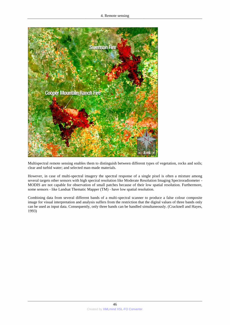
Multispectral remote sensing enables them to distinguish between different types of vegetation, rocks and soils;
clear and turbid water; and selected man-made materials.
However, in case of multi-spectral imagery the spectral response of a single pixel is often a mixture among
several targets other sensors with high spectral resolution like Moderate Resolution Imaging Spectroradiometer -
MODIS are not capable for observation of small patches because of their low spatial resolution. Furthermore,
some sensors - like Landsat Thematic Mapper (TM) - have low spatial resolution.
Combining data from several different bands of a multi-spectral scanner to produce a false colour composite
image for visual interpretation and analysis suffers from the restriction that the digital values of three bands only
can be used as input data. Consequently, only three bands can be handled simultaneously. (Cracknell and Hayes,
1993)

4. Remote sensing
47 Created by XMLmind XSL-FO Converter.
The wavelengths are approximate; exact values depend on the particular satellite's instruments:
• Blue, 450-515..520 nm, used for atmospheric and deep water imaging. Can reach within 150 feet (46 m) deep
in clear water.
• Green, 515..520-590..600 nm, used for imaging of vegetation and deep water structures, up to 90 feet (27 m)
in clear water.
• Red, 600..630-680..690 nm, used for imaging of man-made objects, water up to 30 feet (9.1 m) deep, soil, and
vegetation.
• Near infrared, 750-900 nm, primarily for imaging of vegetation.
• Mid-infrared, 1550-1750 nm, for imaging vegetation and soil moisture content, and some forest fires.
• Mid-infrared, 2080-2350 nm, for imaging soil, moisture, geological features, silicates, clays, and fires.
• Thermal infrared, 10400-12500 nm, uses emitted radiation instead of reflected, for imaging of geological
structures, thermal differences in water currents, fires, and for night studies.
• Radar and related technologies, useful for mapping terrain and for detecting various
objects.(http://en.wikipedia.org/wiki/Multi-spectral_image)
4. 4.3. Hyperspectral
The recent development of hyperspectral sensors and image-data analysing software it is one of the most
significant breakthroughs in remote sensing (Ritvayné et al.. 2009)
Hyperspectral sensors can capture data in contiguous, hundreds of narrow bands in the electromagnetic
spectrum, so presents numerous possibilities for interpretation and analysis. The large numbers of bands provide
for researchers vast quantities of information about the study area. Hyperspectral data can often capture the
unique spectra or ‗spectral signature‘ of an object. This signature can be used to differentiate and identify
materials on the basis of the spectral library provided by analysis softwares like ITT ENVI.
Hyperspectral remote sensing integrates imaging and spectroscopy in a single system which often includes large
data sets due to the fine narrow subdivision of bands and the ―hyper‖ number of bands in the spectrum (Zhou,
2007).
Numerous publications dealt with the analysis of the hyperspectral data regarding to wide range of science area
such as weed pattern analysis (Zhou, 2007; Tamás et al., 2006); acid mine drainage (Szucs et al., 2002; Yan and
Bradshaw, 1995); soil plant systems for characterization of the distribution of heavy metals (Kabata-Pendias,

4. Remote sensing
48 Created by XMLmind XSL-FO Converter.
2001; Faheed, 2005); heavy metal distribution by mapping technologies (Nagy and Tamás, 2008), water
management (Burai and Tamás, 2004) precision agricultural (Tamás et al., 2009).
A lot of sensors have been developed which can provide a near complete spectrum for each pixel using high
spectral resolution. Calibrated hyperspectral data is comparable to laboratory spectra to identify ground
materials at pure or mixed pixels. Sensors used for data acquisition can be installed in both airborne and land
carrier units (Zhou, 2007; Ritvayné et al., 2009). While processing and evaluating information, it is also
necessary to carry out ground measurements and collect reference data using conventional sampling.
After the radiometric and geometric correction, the hyperspectral n-dimensional data cube can be suitable for
classification. This data cube contains all geographical and spectral data changing pixel by pixel.
4.1. Practice 5: Represent spectral profile of an hyperspectral image
1.Start ENVI. Set working folders. Open File menu / Preferences. In the System Preferences window, select the
Default Directories tab. Navigate and choose the Data Directory, which will open automatically at every
operation.

4. Remote sensing
49 Created by XMLmind XSL-FO Converter.
2.Specify the default temp directory for output temporary files.
4.1.1. Exercise 5.1. Display hyperspectral image- true color
3.If an input file has wavelengths for each band stored in the header and the file contains bands in the needed
wavelength ranges, you can display a true color from the Available Bands List without having to designate the
individual bands for red, green, and blue. ENVI displays the true-color image band in the red wavelength region
(0.6-0.7 μm) in red, the band in the green region (0.5-0.6 μm) in green, and the band in the blue region (0.4-0.5
μm) in blue. If the file does not have bands in the needed wavelengths, ENVI uses the bands nearest to the
wavelengths. This may produce a gray scale image if red, green, and blue are set to the same band.
4.In the Available Bands List, right-click on the filename.

4. Remote sensing
50 Created by XMLmind XSL-FO Converter.
5.Select Load True Color to load the image to a new display group if no display groups are open.
6.Select Load True Color to new to load the image to a new display group.
7.Select Load True Color to current to load the image to the active display group.

4. Remote sensing
51 Created by XMLmind XSL-FO Converter.
When you display a file from the Available Bands List, a group of windows will appear on your screen allowing
you to manipulate and analyze your image. This group of windows is collectively referred to as the display
group. The default display group consists of the following:
• Image window: Displays the image at full resolution. If the image is large, the Image window displays the
subsection of the image defined by the Scroll window Image box.
• Zoom window: Displays the subsection of the image defined by the Image window Zoom box. The resolution
is at a user-defined zoom factor based on pixel replication or interpolation.
• Scroll window: Displays the full image at subsampled resolution. This window appears only when an image
is larger than what ENVI can display in the Image window at full resolution.
4.1.2. Exercise 5.2. Display hyperspectral image (RGB)
8.You can open image files or other binary image files of known format. From the main menu bar, select File
menu / Open Image File. When you open a file for the first time during a session, ENVI automatically places the
filename, with all of its associated bands listed beneath it, into the Available Bands List. If a file contains map
information as well, a map icon appears under the filename.
4. Remote sensing
52 Created by XMLmind XSL-FO Converter.
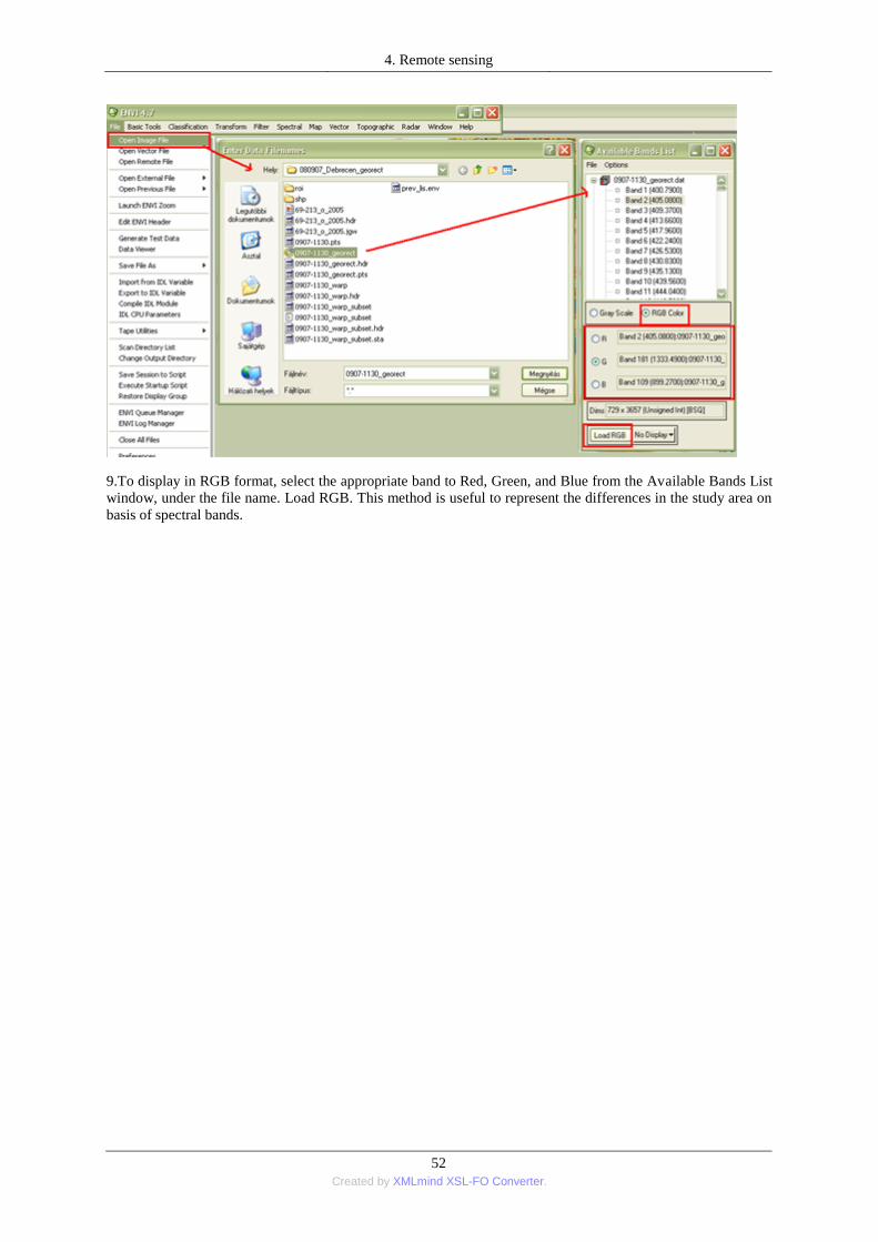
9.To display in RGB format, select the appropriate band to Red, Green, and Blue from the Available Bands List
window, under the file name. Load RGB. This method is useful to represent the differences in the study area on
basis of spectral bands.
4. Remote sensing
53 Created by XMLmind XSL-FO Converter.
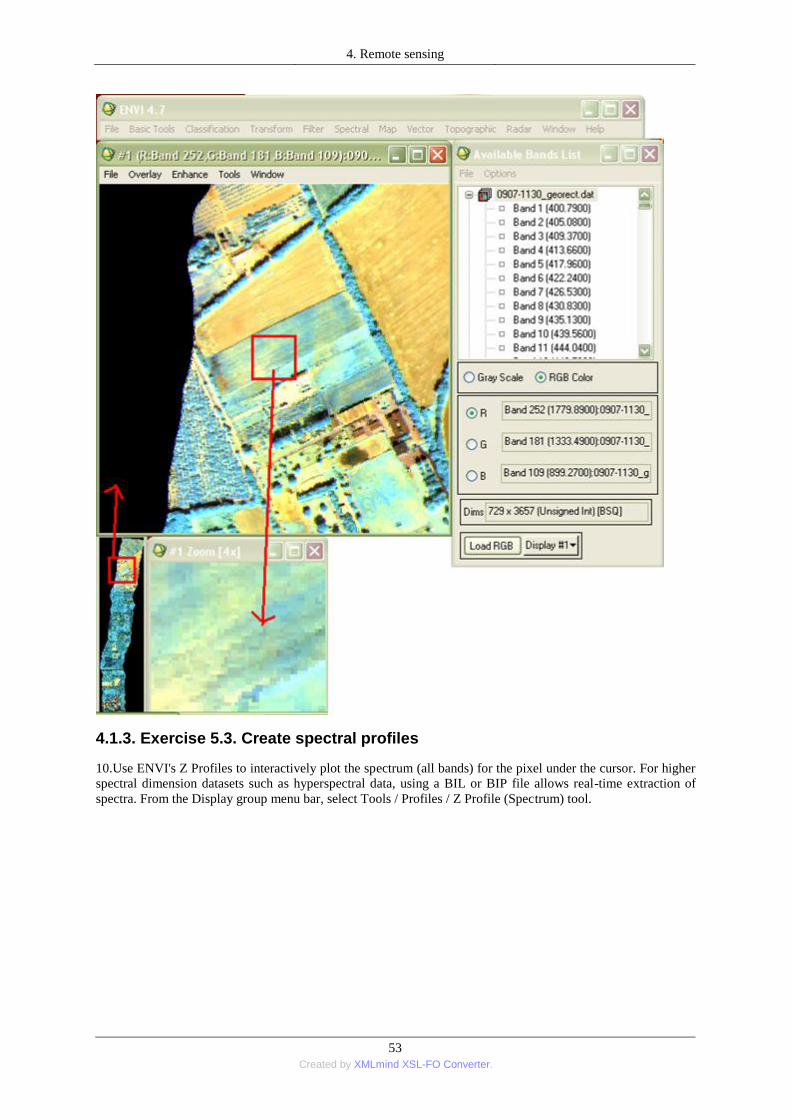
4.1.3. Exercise 5.3. Create spectral profiles
10.Use ENVI's Z Profiles to interactively plot the spectrum (all bands) for the pixel under the cursor. For higher
spectral dimension datasets such as hyperspectral data, using a BIL or BIP file allows real-time extraction of
spectra. From the Display group menu bar, select Tools / Profiles / Z Profile (Spectrum) tool.

4. Remote sensing
54 Created by XMLmind XSL-FO Converter.
11.In the display group, right-click and select Z Profile (Spectrum). Select a pixel in either the Image window or
the Zoom window to plot the corresponding spectrum in the plot window. A vertical line (plot bar) on the plot
marks the wavelength position of the currently displayed band. If a color composite image displays, three colour
lines appear, one for each displayed band in the band's respective color (RGB).
Vertical Plot bars in the Z Profile window show which band or RGB bands are currently displayed in the
window. You can interactively change the bands shown in the window by moving the plot bars to new band
positions.

4. Remote sensing
55 Created by XMLmind XSL-FO Converter.
12.To plot multiple Z Profiles (spectra) over each other in the Spectral Profile plot window, select Options /
Collect Spectra from the Spectral Profile plot window menu bar.
13.From the plot window menu bar, select Edit / Plot Parameters. The Plot Parameters dialog appears.
4.2. Practice 6: Representing of vegetation distribution from hyperspectral data
4.2.1. Exercise 6.1. Calculation vegetation index - NDVI
1.The NDVI (Normalized Difference Vegetation Index) values indicate the amount of green vegetation present
in the pixel. Values of the NDVI index are calculated from the reflected solar radiation in the near-infrared
(NIR) and red (R) wavelength bands, i.e. 580–680 nm, and 730–1100 nm, respectively. NDVI can be
determined using the following formula: NDVI = (NIR – R)/(NIR + R). Higher NDVI values indicate more
green vegetation. Valid results fall between -1 and +1. Before analysis define the wavelength unit of measure of
the hyperspectral image.
2.Select File menu / Edit ENVI Header tool. Choose the hyperspectral image file, OK. In the Header Info
window select the Edit Attribute button / Wavelength tool. In the next dialog window select the units of
wavelength - Nano or micrometer depending on the hyperspectral imagery method.

4. Remote sensing
56 Created by XMLmind XSL-FO Converter.
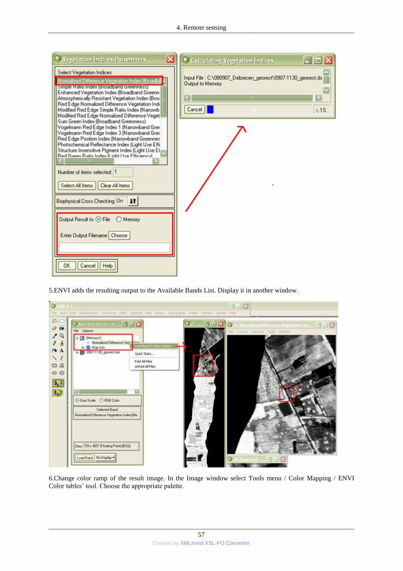
3.From the ENVI main menu bar, select Spectral menu / Vegetation Analysis / Vegetation Index Calculator tool.
The Input File dialog appears.
4.Specify the Input File Type from the drop-down list. OK. ENVI automatically enters the bands it uses to
calculate the NDVI in the Red and Near IR fields. Select the Normalized Difference Vegetation Index – NDVI
from the list of vegetation indices. Select output to File or Memory. Click OK.
4. Remote sensing
57 Created by XMLmind XSL-FO Converter.
5.ENVI adds the resulting output to the Available Bands List. Display it in another window.
6.Change color ramp of the result image. In the Image window select Tools menu / Color Mapping / ENVI
Color tables‘ tool. Choose the appropriate palette.

4. Remote sensing
58 Created by XMLmind XSL-FO Converter.
7.Add Legend to map. In the image window select the Overlay menu / Annotation tool, then select Object menu
/ Color ramp tool in the Annotation window. Select the parameters of the legend – such as placement, font type,
orientation, and the scale. Click in the select window to display the legend.
4.2.2. Exercise 6.2. Export data to ArcMap
To open data in ArcMap™ software, you must have ArcMap version 9.2 or higher installed and licensed on
your system.

4. Remote sensing
59 Created by XMLmind XSL-FO Converter.
8.Click File menu / Export Image to ArcMap from the display group menu bar to export the image in the display
group to ArcMap software, including any associated display enhancements and annotations. This menu option is
only available on Windows 32-bit platforms or when running ENVI in 32-bit mode on Windows. When you
select this option, ENVI converts the full extent of the image in the display group (including display
enhancements, annotation, contrast stretches, etc.) to a three-band GeoTIFF file and saves it in the location you
specify as the Temp Directory of your ENVI System Preferences. ArcMap software then displays this image
These exercises were worked out for practical purposes used by ENVI Version 4.7 (2009) Copyright © ITT
Visual Information Solutions.

60 Created by XMLmind XSL-FO Converter.
5. fejezet - 5. Agricultural application of remote sensing data
1.
The remote sensing data is widely used in agriculture (Tamás and Lénárt, 2006).
Moderate Resolution Imaging Spectroradiometer - MODIS are not capable for observation of small patches
because of their low spatial resolution, but data provided MODIS are suitable for global examination. The prior
probabilities for agriculture (class 12) and agricultural mosaic (class 14) are replaced with probabilities
parameterized using the dataset produced by (Ramankutty et al., 2008), which furnishes estimates of global
cropping intensity at 0.05° spatial resolution (roughly 30 km2 at the equator) for year 2000. The picture shows
the global distribution of the resulting prior probabilities for the agriculture and agricultural mosaic classes.
(Friedl et al., 2010)
The LIDAR (Light Detection And Ranging) has been used to measure environmental or ecological parameters
of plantations such as the structural characteristics of surface, features, or fruit trees. In recent years, a new
technology - the line scanning mechanism – can supply good results about plantations.
5. Agricultural application of remote
sensing data
61 Created by XMLmind XSL-FO Converter.
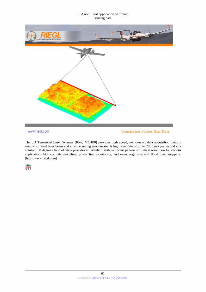
The 3D Terrestrial Laser Scanner (Riegl VZ-100) provides high speed, non-contact data acquisition using a
narrow infrared laser beam and a fast scanning mechanism. A high scan rate of up to 200 lines per second at a
constant 60 degrees field of view provides an evenly distributed point pattern of highest resolution for various
applications like e.g. city modeling, power line monitoring, and even large area and flood plain mapping.
(http://www.riegl.com)

5. Agricultural application of remote
sensing data
62 Created by XMLmind XSL-FO Converter.

5. Agricultural application of remote
sensing data
63 Created by XMLmind XSL-FO Converter.
The first uses of airborne mapping LiDAR were as profiling altimeters by the U.S. military in the mid 1960‘s,
and included the recording transects of Arctic ice packs and detecting submarines. The first results of
topographic mapping with this system were reported in 1984. The basics of airborne mapping LiDAR are
illustrated with Figure 5.6. The core of a system is a laser source that emits pulses of laser energy with a typical
duration of a few nanoseconds (10-9 s) and that repeats several thousands of times per second (kHz) in what is
called pulse repetition frequency (PRF). The laser pulses are distributed in two dimensions over the area of
interest. The first dimen¬sion is along the airplane flight direction and is achieved by the forward motion of the
aircraft. The second dimension is obtained using a scanning mechanism, which is most often an oscillating
mirror that steers the laser beam side-to-side perpendicular to the line of flight. The combination of the aircraft
motion and the optical scanning distributes the laser pulses over the ground in a saw tooth pattern. The selected
scanning angle and flying height determine the swath width. The scanning frequency, in conjunction with the
PRF, determines the across-track spacing of the laser pulses, or the cross-track resolution. The aircraft ground
speed and scan frequency determines the down-track resolution. (Fernandez Diaz, J. C., 2011)
Figure 5.7. illustrates that the laser energy spreads in a conical fashion as it propa¬gates through the atmosphere,
similar to the pattern of a highly directive spotlight. This spread is determined by the laser beam divergence and,
in conjunction with the flying height, defines the size of the beam footprint on the ground. Some airborne
systems, such as NASA's Laser Vegetation Imaging Sensor (LVIS), have large footprints of 10-30 m in
diameter as they are used to simulate or validate space borne LiDAR sensors. However, most commercial
airborne LiDAR units are characterized by beam divergences that produce footprints between 15-90 cm from
their typical operational altitudes, and thus are considered "small footprint" systems. Figure 5.7. also illustrates a
time-versus-intensity plot, or waveform of a laser pulse propagating in time at the speed of light. When the pulse
exits the sensor, it gener¬ally has a nearly Gaussian profile. As the light interacts with the trees or the ground,
some of the energy is reflected back towards the sensor, modifying the wave¬form shape according to the
geometric properties of the target. The reflected photons are registered by a photo detector, and the signal
generated can be recorded continuously for posterior analysis, as in the case of waveform digitizing systems, or

5. Agricultural application of remote
sensing data
64 Created by XMLmind XSL-FO Converter.
can be analyzed on-the-fly by elec¬tronics that provide precise timing tags of specific waveform features, as in
the case of discrete recording systems. From the analysis of the waveform or the time tags, the two-way flight
times between the sensor and the reflective surfaces that the laser pulses encounter along the path are
determined. Dividing these time intervals (time of flight) by 2 and multiplying by the speed of light yields the
slant range to the reflective surfaces.
In order to determine coordinates for each laser return event, in addi¬tion to the range and scan angle, it is
necessary to know the airplane's posi¬tion and orientation (trajectory). This is achieved by an integrated
navigation system (INS) that processes observations of an IMU and global naviga¬tion satellite system (GNSS).
The IMU is comprised of triads of accelerometers and gyroscopes that record the linear and angular
accelerations of the aircraft. The GNSS observations are carrier phase measurements collected from both the
aircraft and fixed ground reference stations, which are processed differentially post mission. (Fernandez Diaz, J.
C., 2011)
The unique combination of wave¬length, beam divergence and scanning capability allows the laser energy to
penetrate through the canopy on its way to the ground and back to the sensor. The waveforms are analyzed
along their entire reflection path to isolate the last laser return. These last returns obtained from waveform or
discrete LiDAR are collectively analyzed over a given area using 3D morphological filters to classify the returns
as coming from the ground or other objects. This spatial classification allows the removal of the canopy to
obtain digital elevation models (DEM) of the bare surface revealing geological features or manmade structures
hidden under the forest structure. (Fernandez Diaz, J. C., 2011)
Airborne remote sensing data are increasingly used in precision agriculture. Applicability of Remote Sensing
data is mostly depending on the spatial and spectral resolution. Nowadays, a new generation of airborne
hyperspectral imaging systems is available and applicable to map the environment. (Tamás et al., 2009)

5. Agricultural application of remote
sensing data
65 Created by XMLmind XSL-FO Converter.
The AISA DUAL hyperspectral imaging system consists of two sensor sensing with 0.5m ground resolution.
AISA is a dual sensor system, which provides seamless hyperspectral data in the full range of 400 - 2500nm.
The Eagle camera can take images in (VNIR) the visible and near infrared range (400- 1300 nm), while Hawk
can be used to analyze in shortwave infrared, with spectral ranges of 1300 nm to 1900nm (SWIR-1) and
1900nm to 2500 nm (SWIR-2) with 498 spectral channels. The AISA system included push broom imaging
sensors, consisting of a hyperspectral and high-performance GPS/INS sensor and a data acquisition unit housed
in a rugged PC.
A real-time fiber optic down welling irradiance sensor (FODIS) on top of pilot cabin was integrated into the
sensors to monitor the illumination conditions. Auxiliary components included a mount to connect the sensor to
the GPS/INS unit, and regulated the power supply.
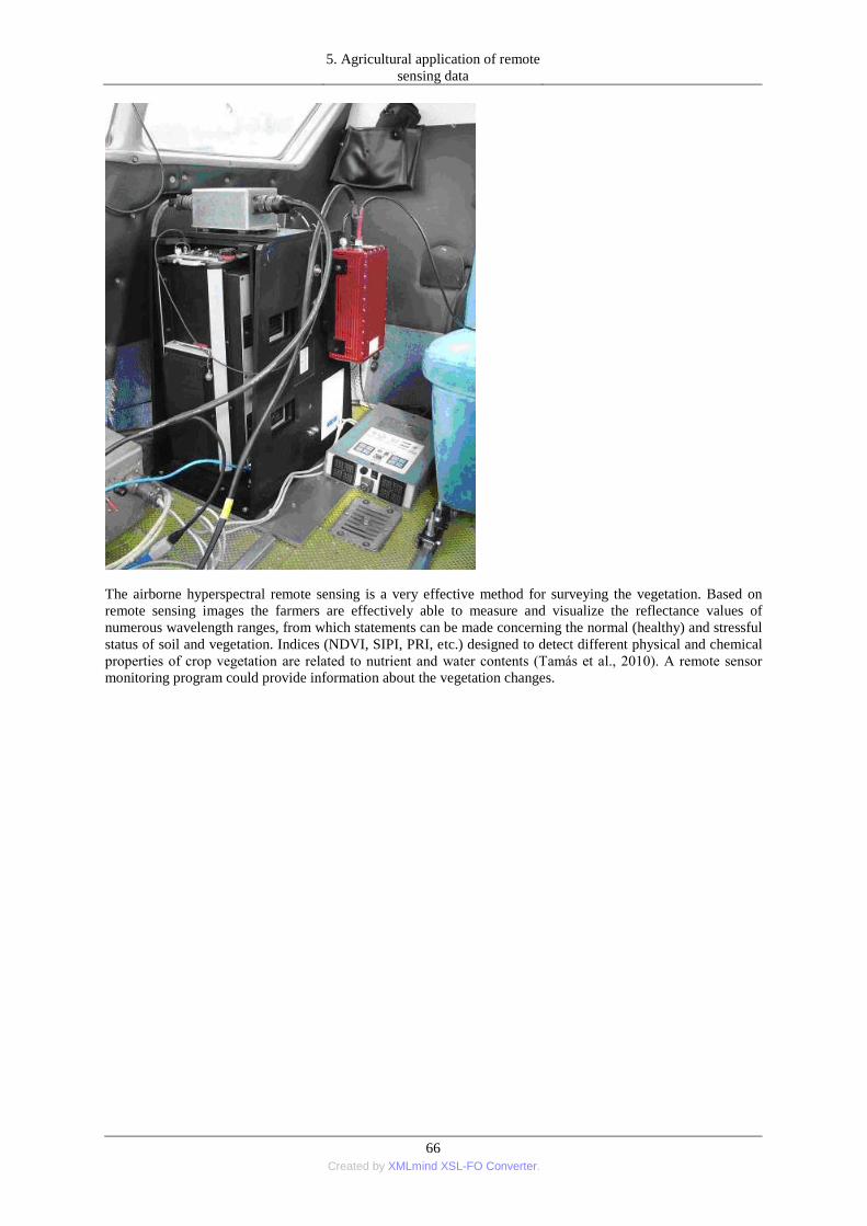
5. Agricultural application of remote
sensing data
66 Created by XMLmind XSL-FO Converter.
The airborne hyperspectral remote sensing is a very effective method for surveying the vegetation. Based on
remote sensing images the farmers are effectively able to measure and visualize the reflectance values of
numerous wavelength ranges, from which statements can be made concerning the normal (healthy) and stressful
status of soil and vegetation. Indices (NDVI, SIPI, PRI, etc.) designed to detect different physical and chemical
properties of crop vegetation are related to nutrient and water contents (Tamás et al., 2010). A remote sensor
monitoring program could provide information about the vegetation changes.

5. Agricultural application of remote
sensing data
67 Created by XMLmind XSL-FO Converter.
Besides, the reflectance value of the vegetation without any stress is high at NIR intervals, but low at red
wavelength interval. The chlorophyll content is one of the indicators of the state of health before ripening
phenological phase (Burai et al. 2009).
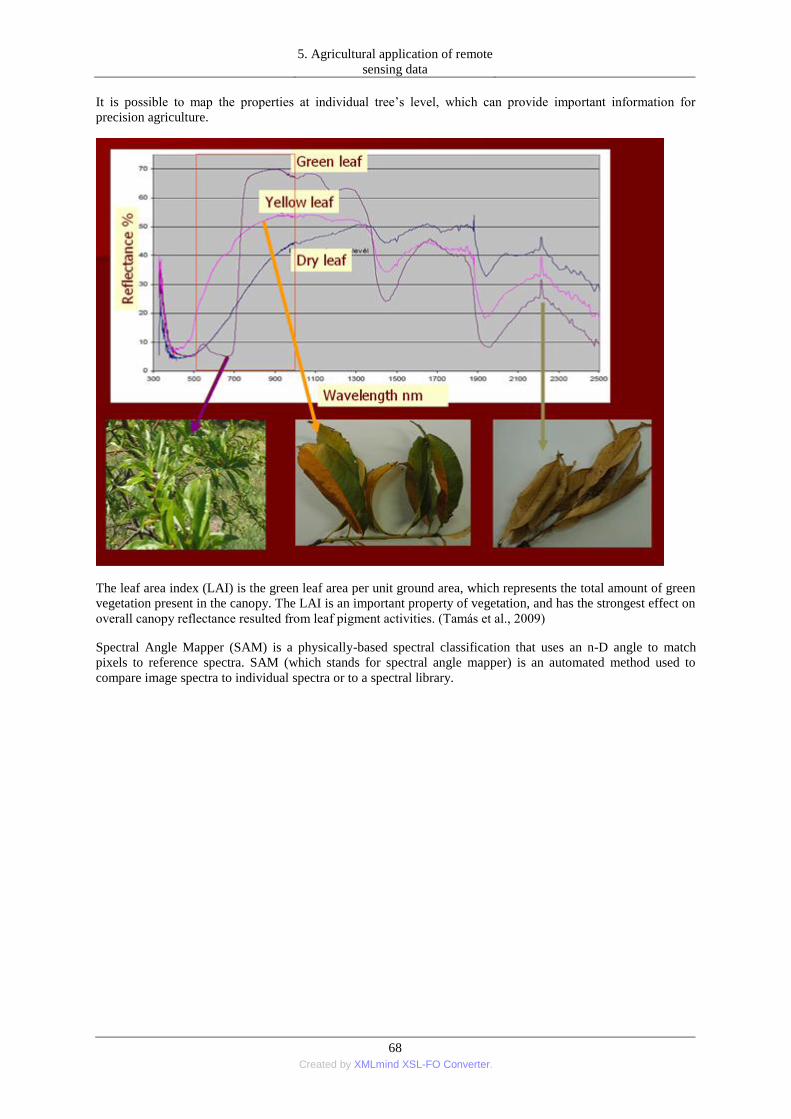
5. Agricultural application of remote
sensing data
68 Created by XMLmind XSL-FO Converter.
It is possible to map the properties at individual tree‘s level, which can provide important information for
precision agriculture.
The leaf area index (LAI) is the green leaf area per unit ground area, which represents the total amount of green
vegetation present in the canopy. The LAI is an important property of vegetation, and has the strongest effect on
overall canopy reflectance resulted from leaf pigment activities. (Tamás et al., 2009)
Spectral Angle Mapper (SAM) is a physically-based spectral classification that uses an n-D angle to match
pixels to reference spectra. SAM (which stands for spectral angle mapper) is an automated method used to
compare image spectra to individual spectra or to a spectral library.
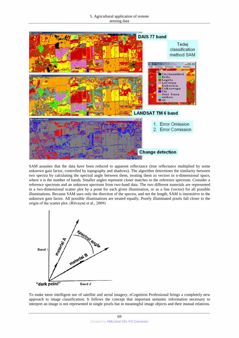
5. Agricultural application of remote
sensing data
69 Created by XMLmind XSL-FO Converter.
SAM assumes that the data have been reduced to apparent reflectance (true reflectance multiplied by some
unknown gain factor, controlled by topography and shadows). The algorithm determines the similarity between
two spectra by calculating the spectral angle between them, treating them as vectors in n-dimensional space,
where n is the number of bands. Smaller angles represent closer matches to the reference spectrum. Consider a
reference spectrum and an unknown spectrum from two-band data. The two different materials are represented
in a two-dimensional scatter plot by a point for each given illumination, or as a line (vector) for all possible
illuminations. Because SAM uses only the direction of the spectra, and not the length, SAM is insensitive to the
unknown gain factor. All possible illuminations are treated equally. Poorly illuminated pixels fall closer to the
origin of the scatter plot. (Ritvayné et al., 2009)
To make more intelligent use of satellite and aerial imagery, eCognition Professional brings a completely new
approach to image classification: It follows the concept that important semantic information necessary to
interpret an image is not represented in single pixels but in meaningful image objects and their mutual relations.

5. Agricultural application of remote
sensing data
70 Created by XMLmind XSL-FO Converter.
The basic difference, especially when compared with pixel-based procedures is that eCognition does not classify
single pixels but rather image objects which are extracted in a previous image segmentation step. (White Paper
eCognition Professional 4.0)
The pixels of the associated region are linked to the image object with an is-part-of link object. Two image
objects are neighbouring each other if their associated regions are neighbouring each other according to the
selected pixel neighbourhood. An image is segmented into image objects. All together, the image objects of a
segmentation procedure form an image object level. Two or more image object levels build the image object
hierarchy. An astonishing characteristic of object-oriented image analysis is the amount of additional
information which can be derived from image objects and thus used for classification: tone, shape, texture, area,
context, and information from other object layers. The image object domain is defined by a structural
description of the corresponding subset. Examples for image object domains are the entire image, an image
object level or all image objects of a given class. (eCognition Professional 4.0 User Guide)
ENVI Zoom is a powerful viewer with a dynamic display that allows for rapid viewing and manipulation of
remotely sensed images, vectors, and annotations. The interface provides quick access to common display tools
such as contrast, brightness, sharpening, and transparency. ENVI Zoom also contains the robust RX Anomaly
Detection, Pan Sharpening, and Vegetation Suppression tools. The RX Anomaly Detection tool detects spectral
or color differences between layers and extracts unknown targets that are spectrally distinct from the image
background. Use Pan Sharpening to sharpen low spatial resolution multispectral data using high spatial
resolution panchromatic data. The Vegetation Suppression tool allows you to remove the vegetation spectral
signature from multispectral and hyperspectral imagery. (ENVI Zoom© ITT Visual Information Solutions)
1.1. Practice 7: Create spectral scatter plot
1.1.1. Exercise 7.1. 2D Scatter Plots interactive classification
If desired, you can have multiple scatter plots active simultaneously. Two-dimensional scatter plots use only the
data in the Image window so quick interactive response is provided. You can also show the density distribution
of the scatter plot.
1.From the Image window (Display group) menu bar, select Tools menu / 2D Scatter Plots. The Scatter Plot
Band Choice dialog appears.
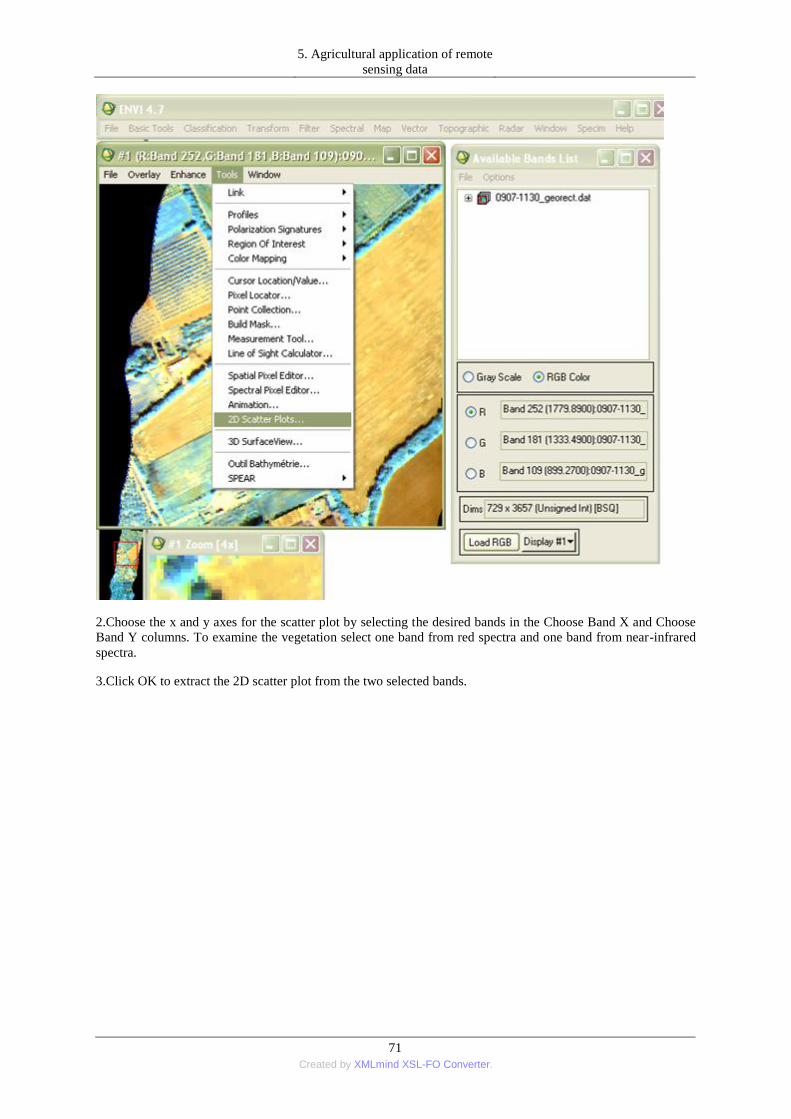
5. Agricultural application of remote
sensing data
71 Created by XMLmind XSL-FO Converter.
2.Choose the x and y axes for the scatter plot by selecting the desired bands in the Choose Band X and Choose
Band Y columns. To examine the vegetation select one band from red spectra and one band from near-infrared
spectra.
3.Click OK to extract the 2D scatter plot from the two selected bands.

5. Agricultural application of remote
sensing data
72 Created by XMLmind XSL-FO Converter.
As soon as the scatter plot appears, the interactive scatter plot function is available for use.
You can draw ROIs in the scatter plot to provide an interactive classification method.
4.In the Scatter plot window, left-click at the vertices of a polygon enclosing the desired region. Right-click to
close the polygon and complete the selection. When the region is closed, all pixels in the image that fall within
the DN range of those selected in the scatter plot are highlighted in color in the Image window. Select Class
menu / New tool to draw another polygon selection, right-click to close.

5. Agricultural application of remote
sensing data
73 Created by XMLmind XSL-FO Converter.
1.1.2. Exercise 7.2. Creation of ROI
Before SAM classification the regions of interest (ROIs) has to be defined. You can select graphically or by
other means, such as thresholding. Typical uses of ROIs include extracting statistics for classification, masking,
and other functions. You can use any combination of polygons, points, or vectors as an ROI. ENVI allows you
to define multiple ROIs and draw them in any of the Image, Scroll, or Zoom windows. In addition, you can
grow ROIs to adjacent pixels that fall within a specified pixel value threshold.
1.Select one of the following options for the active display group:
• From the Display group menu bar, select Overlay menu / Region of Interest tool
• From the Display group menu bar, select Tools menu / Region of Interest / ROI Tool
• From the ENVI main menu bar, select Basic Tools menu / Region of Interest / ROI Tool
• In the display group, right-click and select ROI Tool
The ROI Tool dialog appears.
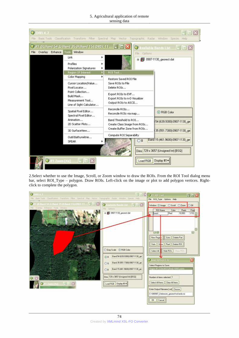
5. Agricultural application of remote
sensing data
74 Created by XMLmind XSL-FO Converter.
2.Select whether to use the Image, Scroll, or Zoom window to draw the ROIs. From the ROI Tool dialog menu
bar, select ROI_Type – polygon. Draw ROIs. Left-click on the image or plot to add polygon vertices. Right-
click to complete the polygon.

5. Agricultural application of remote
sensing data
75 Created by XMLmind XSL-FO Converter.
3.From the ROI Tool dialog menu bar, select File menu / Save ROIs. Enter a filename. This process has to be
repeated several times, while the classification we need different ROI of the study areas such as forest, dry
vegetation, green vegetation, buildings, water surface.
1.2. Practice 8: Classification methods
1.2.1. Exercise 8.1. n-D Visualizer
The n-D Visualizer helps to locate, identify, and cluster the purest pixels and the most extreme spectral
responses in a dataset. You can visualize the shape of a data cloud that results from plotting image data in
spectral space (with image bands as plot axes). The n-D Visualizer is an interactive tool to use for selecting the
endmembers in n-D space. When using the n-D Visualizer, you can interactively rotate data in n-D space, select
groups of pixels into classes, and collapse classes to make additional class selections easier. You can export the
selected classes to ROIs and use them as input into classification, Linear Spectral Unmixing, or Matched
Filtering techniques.
1.From the ENVI main menu bar, select Spectral menu / n-Dimensional Visualizer / Visualize with New Data
tool. The Input File dialog appears.
2.This process needs ROIs. Create ROIs on the basis of above mentioned method.
3.Select the ROI to use.

5. Agricultural application of remote
sensing data
76 Created by XMLmind XSL-FO Converter.
4.The n-D Visualizer and n-D Controls dialogs appear. The n-D Controls dialog contains representations of all
of the bands that you selected during the file selection. The bands are represented by numbered boxes that
initially appear black. Clicking an individual band number in the n-D Controls dialog turns the band number
white and displays the corresponding band pixel data in the n-D scatter plot. You must select at least two bands
to view a scatter plot. You can select any combination of bands at once. Clicking the same band number again
turns it black and turns off the band pixel data in the n-D scatter plot.
5.Enter a Speed value in the n-D Controls dialog. Higher values cause faster rotation with fewer steps between
views. Click Start or Stop in the n-D Controls dialog box to start or stop the rotation.

5. Agricultural application of remote
sensing data
77 Created by XMLmind XSL-FO Converter.
6.You can turn the axes on or off in the n-D Visualizer, Select Options menu / Show Axes tool from the n-D
Controls menu bar.
7.When using the n-D Visualizer, your goal is to visually identify and distinguish the purest pixels in the image.
Each corner corresponds to one spectrally unique material in the image. Therefore, you should try to find all the
corners of the data cloud and assign each corner a different color. Set vertices left-clicking on the n-dimensional
panel, and right-clicking to close the polygon. Use the Z Profile option to help define classes.
1.2.2. Exercise 8.2. Spectral Angle Mapper Classification
The algorithm determines the spectral similarity between two spectra by calculating the angle between the
spectra and treating them as vectors in a space with dimensionality equal to the number of bands. This
technique, when used on calibrated reflectance data, is relatively insensitive to illumination and albedo effects.
SAM compares the angle between the endmember spectrum vector and each pixel vector in n-D space. SAM
classification assumes reflectance data.
4.From the ENVI main menu bar, select Classification menu / Supervised / Spectral Angle Mapper tool. The
Input File dialog appears.
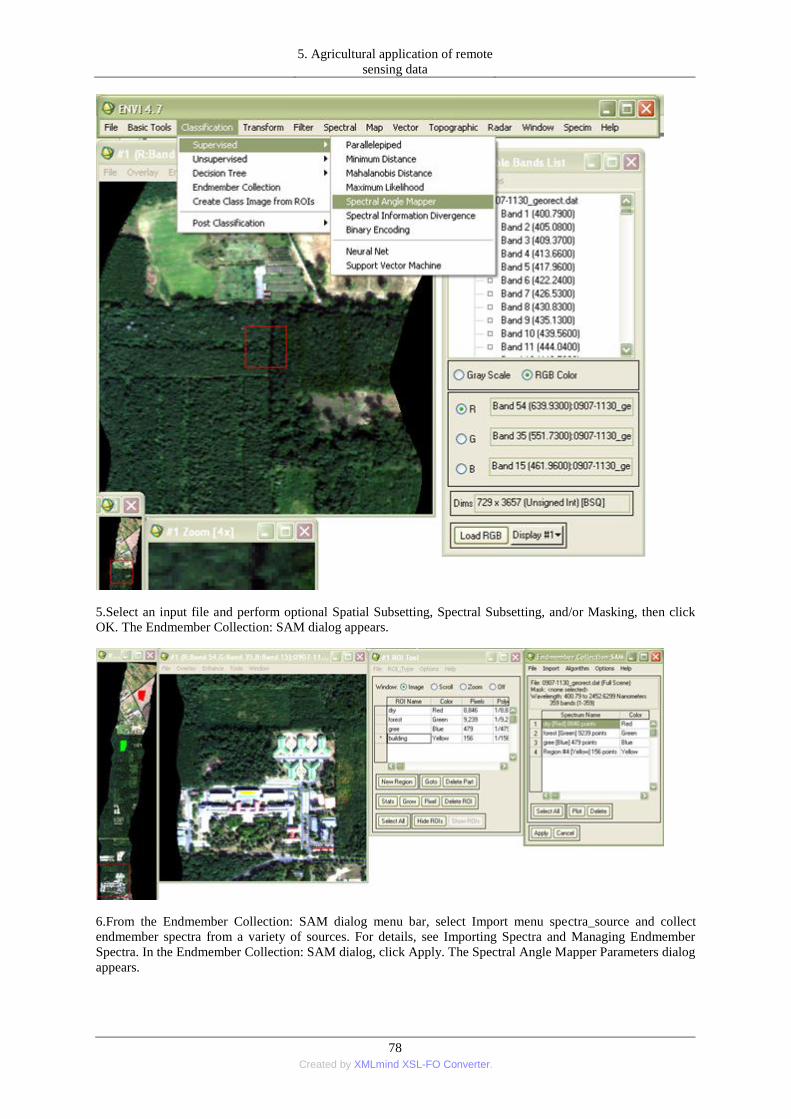
5. Agricultural application of remote
sensing data
78 Created by XMLmind XSL-FO Converter.
5.Select an input file and perform optional Spatial Subsetting, Spectral Subsetting, and/or Masking, then click
OK. The Endmember Collection: SAM dialog appears.
6.From the Endmember Collection: SAM dialog menu bar, select Import menu spectra_source and collect
endmember spectra from a variety of sources. For details, see Importing Spectra and Managing Endmember
Spectra. In the Endmember Collection: SAM dialog, click Apply. The Spectral Angle Mapper Parameters dialog
appears.
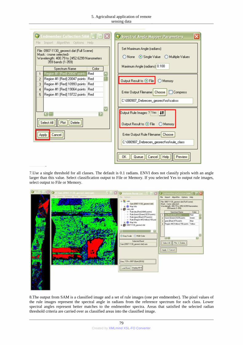
5. Agricultural application of remote
sensing data
79 Created by XMLmind XSL-FO Converter.
7.Use a single threshold for all classes. The default is 0.1 radians. ENVI does not classify pixels with an angle
larger than this value. Select classification output to File or Memory. If you selected Yes to output rule images,
select output to File or Memory.
8.The output from SAM is a classified image and a set of rule images (one per endmember). The pixel values of
the rule images represent the spectral angle in radians from the reference spectrum for each class. Lower
spectral angles represent better matches to the endmember spectra. Areas that satisfied the selected radian
threshold criteria are carried over as classified areas into the classified image.

5. Agricultural application of remote
sensing data
80 Created by XMLmind XSL-FO Converter.
Smaller angles represent closer matches to the reference spectrum. Pixels further away than the specified
maximum angle threshold in radians are not classified.
These exercises were worked out for practical purposes used by ENVI Version 4.7 (2009) Copyright © ITT
Visual Information Solutions.
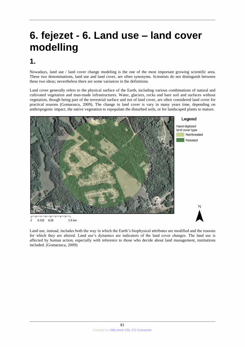
81 Created by XMLmind XSL-FO Converter.
6. fejezet - 6. Land use – land cover modelling
1.
Nowadays, land use / land cover change modeling is the one of the most important growing scientific area.
These two denominations, land use and land cover, are often synonyms. Scientists do not distinguish between
these two ideas; nevertheless there are some variances in the definitions.
Land cover generally refers to the physical surface of the Earth, including various combinations of natural and
cultivated vegetation and man-made infrastructures. Water, glaciers, rocks and bare soil and surfaces without
vegetation, though being part of the terrestrial surface and not of land cover, are often considered land cover for
practical reasons (Gomarasca, 2009). The change in land cover is vary in many years time, depending on
anthropogenic impact, the native vegetation to repopulate the disturbed soils, or for landscaped plants to mature.
Land use, instead, includes both the way in which the Earth‘s biophysical attributes are modified and the reasons
for which they are altered. Land use‘s dynamics are indicators of the land cover changes. The land use is
affected by human action, especially with reference to those who decide about land management, institutions
included. (Gomarasca, 2009)

6. Land use – land cover modelling
82 Created by XMLmind XSL-FO Converter.
For the land use / land cover change analysis topographic map, aerial photo, historical map are used to
determine the spatial extent of the patches and the time of the changes. Orthophotography is very capable of
producing large-scale map sheets too. However, it can be relatively expensive for certain applications. This is as
compared to other, traditional data acquisition methods such as field sampling and field mapping.
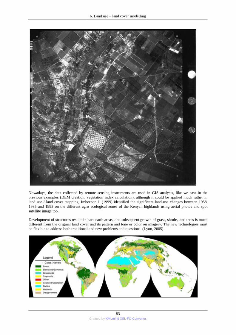
6. Land use – land cover modelling
83 Created by XMLmind XSL-FO Converter.
Nowadays, the data collected by remote sensing instruments are used in GIS analysis, like we saw in the
previous examples (DEM creation, vegetation index calculation), although it could be applied much rather in
land use / land cover mapping. Imbernon J. (1999) identified the significant land-use changes between 1958,
1985 and 1995 on the different agro ecological zones of the Kenyan highlands using aerial photos and spot
satellite image too.
Development of structures results in bare earth areas, and subsequent growth of grass, shrubs, and trees is much
different from the original land cover and its pattern and tone or color on imagery. The new technologies must
be flexible to address both traditional and new problems and questions. (Lyon, 2005)
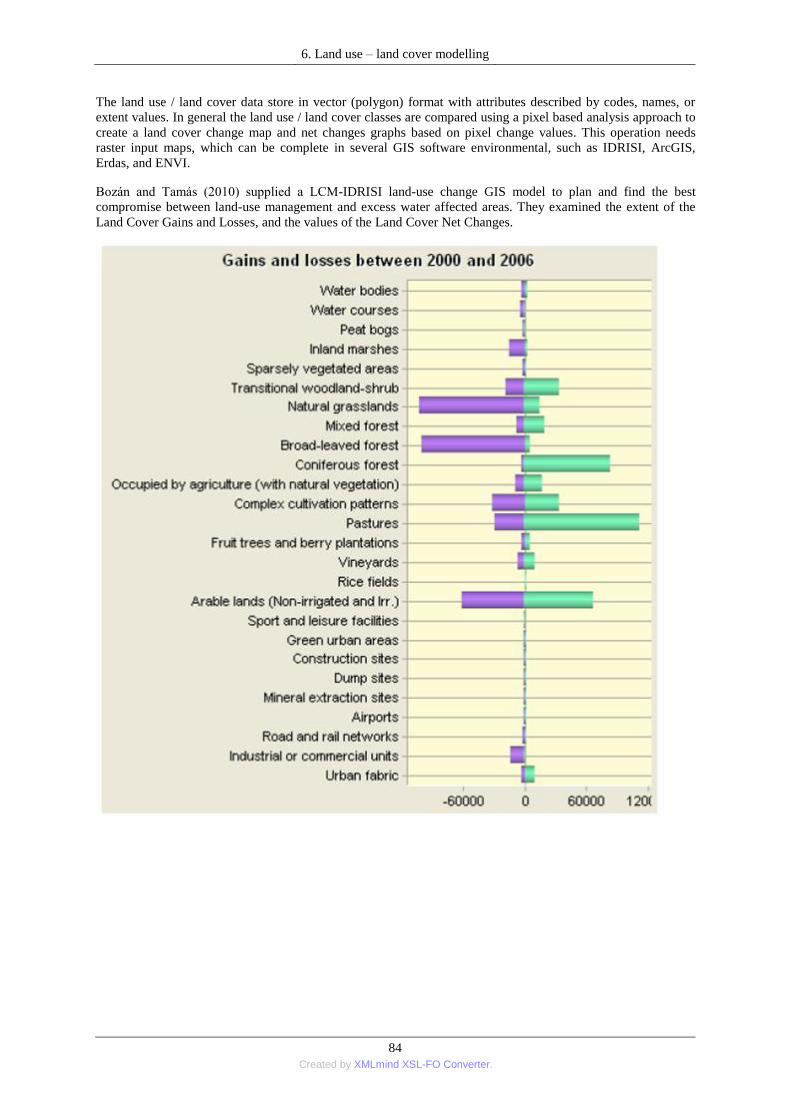
6. Land use – land cover modelling
84 Created by XMLmind XSL-FO Converter.
The land use / land cover data store in vector (polygon) format with attributes described by codes, names, or
extent values. In general the land use / land cover classes are compared using a pixel based analysis approach to
create a land cover change map and net changes graphs based on pixel change values. This operation needs
raster input maps, which can be complete in several GIS software environmental, such as IDRISI, ArcGIS,
Erdas, and ENVI.
Bozán and Tamás (2010) supplied a LCM-IDRISI land-use change GIS model to plan and find the best
compromise between land-use management and excess water affected areas. They examined the extent of the
Land Cover Gains and Losses, and the values of the Land Cover Net Changes.

6. Land use – land cover modelling
85 Created by XMLmind XSL-FO Converter.
The analysis of the spatial extent and temporal change of land-use categories using remotely sensed data is also
of critical importance to agricultural sciences (Tamás, 2003).
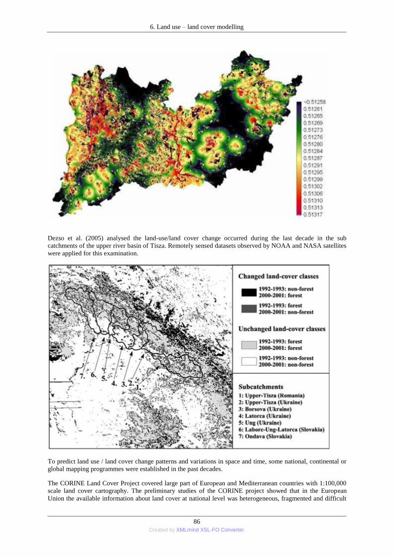
6. Land use – land cover modelling
86 Created by XMLmind XSL-FO Converter.
Dezso et al. (2005) analysed the land-use/land cover change occurred during the last decade in the sub
catchments of the upper river basin of Tisza. Remotely sensed datasets observed by NOAA and NASA satellites
were applied for this examination.
To predict land use / land cover change patterns and variations in space and time, some national, continental or
global mapping programmes were established in the past decades.
The CORINE Land Cover Project covered large part of European and Mediterranean countries with 1:100,000
scale land cover cartography. The preliminary studies of the CORINE project showed that in the European
Union the available information about land cover at national level was heterogeneous, fragmented and difficult

6. Land use – land cover modelling
87 Created by XMLmind XSL-FO Converter.
to find. The origin of the project goes back to June 27, 1985 when, as suggested by the European Union (EU),
the Council approved the CORINE programme, an acronym of Coordination of Information on Environment,
experimental project for the collection, coordination and realization of information on the state of environment
and natural resources within the Community (GU L 176 of 6.7.1985). The methodology is described by the
technical guide drawn up by European Commission‘s experts. (European Environmental Agency, CORINE
Land Cover Project, CORINE land cover technical guide)
CORINE Land Cover programme includes LANDSAT 5 TM images, which are radiometrically corrected and
geo-referred, and/or SPOT XS sensors interpretation. The images sensed in 1990-92 were processed before
being distributed to the photo-interpreters by the Hungarian Institute of Geodesy, Cartography and Remote
Sensing (FÖMI). The database includes 44 categories in accordance with a standard European nomenclature.
The land cover information is stored in topological structure as ARC/INFO database. The project (CLC100,
CLC50) started in 1993 in Hungary. (http://fomi.hu)

6. Land use – land cover modelling
88 Created by XMLmind XSL-FO Converter.
The CORINE Land Cover update to the year 2000 (CLC2000), called Image and Corine Land Cover 2000
project (ICLC2000), schedules the acquisition of remotely sensed Landsat 7 ETM+ images (Image 2000), the
production of the geographical database of land cover for the year 2000 and the assessment of the land
cover/land use changes between the years 1990 and 2000 (CLC-change). The CLC2000 database covers 32
countries.
The area of the smallest mapped patch is 25 hectares, and the maximum error value is 25 meters.
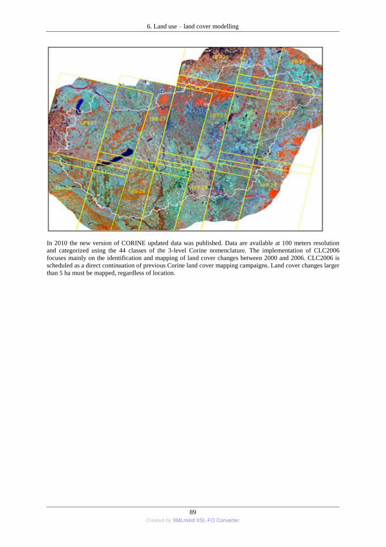
6. Land use – land cover modelling
89 Created by XMLmind XSL-FO Converter.
In 2010 the new version of CORINE updated data was published. Data are available at 100 meters resolution
and categorized using the 44 classes of the 3-level Corine nomenclature. The implementation of CLC2006
focuses mainly on the identification and mapping of land cover changes between 2000 and 2006. CLC2006 is
scheduled as a direct continuation of previous Corine land cover mapping campaigns. Land cover changes larger
than 5 ha must be mapped, regardless of location.
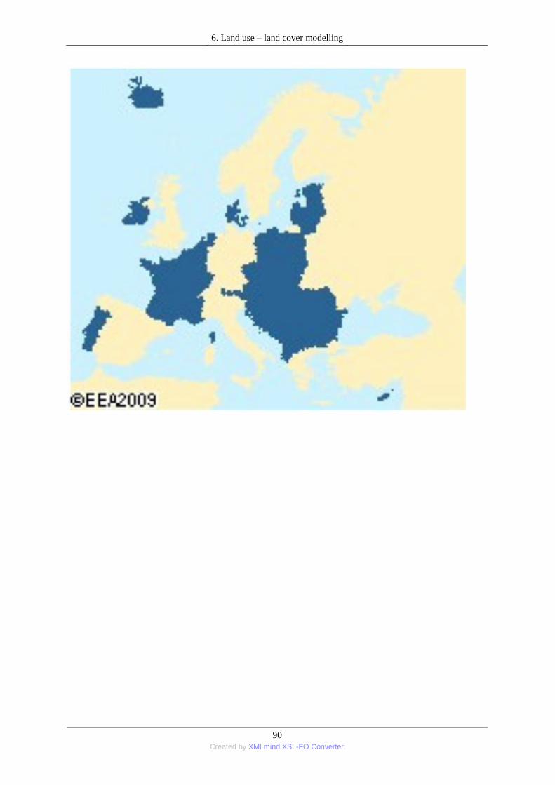
6. Land use – land cover modelling
90 Created by XMLmind XSL-FO Converter.

6. Land use – land cover modelling
91 Created by XMLmind XSL-FO Converter.

6. Land use – land cover modelling
92 Created by XMLmind XSL-FO Converter.
In Spring 2002, the Food and Agriculture Organization of the United Nations (FAO) and the United Nations
Environment Programme (UNEP) launched the Global Land Cover Network (GLCN) with the objective to
improve the availability of global information on land cover and its dynamics, harmonizing land cover mapping
and monitoring at national, regional and global levels. Global Land Cover Network (GLCN) is increasing the
availability of usable and standardized information about land cover with the possibility of interchange at a
global level. In this project more than 30 research teams have been involved, contributing to 19 regional
windows, each mapped by local experts for an accurate classification based on local knowledge. Each regional
partner used the Land Cover Classification System (LCCS) produced by FAO and UNEP, which ensured that a
standard legend was used over the globe. In collaboration with a network of international partners from around
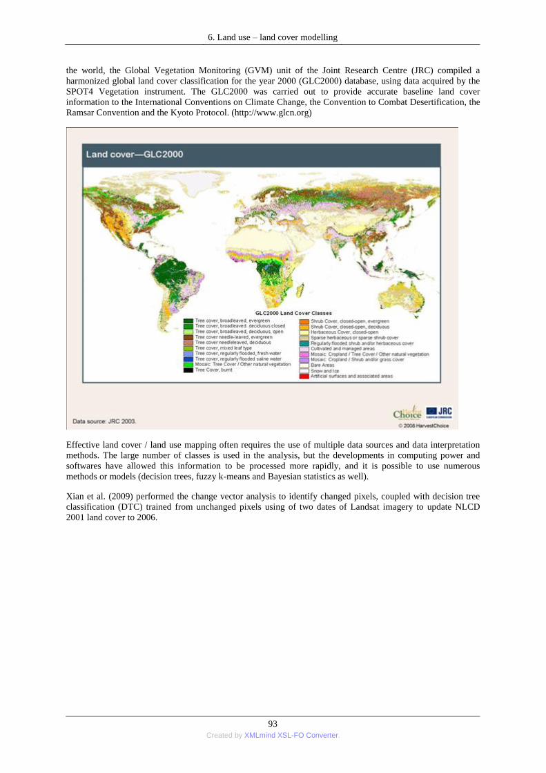
6. Land use – land cover modelling
93 Created by XMLmind XSL-FO Converter.
the world, the Global Vegetation Monitoring (GVM) unit of the Joint Research Centre (JRC) compiled a
harmonized global land cover classification for the year 2000 (GLC2000) database, using data acquired by the
SPOT4 Vegetation instrument. The GLC2000 was carried out to provide accurate baseline land cover
information to the International Conventions on Climate Change, the Convention to Combat Desertification, the
Ramsar Convention and the Kyoto Protocol. (http://www.glcn.org)
Effective land cover / land use mapping often requires the use of multiple data sources and data interpretation
methods. The large number of classes is used in the analysis, but the developments in computing power and
softwares have allowed this information to be processed more rapidly, and it is possible to use numerous
methods or models (decision trees, fuzzy k-means and Bayesian statistics as well).
Xian et al. (2009) performed the change vector analysis to identify changed pixels, coupled with decision tree
classification (DTC) trained from unchanged pixels using of two dates of Landsat imagery to update NLCD
2001 land cover to 2006.

6. Land use – land cover modelling
94 Created by XMLmind XSL-FO Converter.
Aitkenhead and Aalders (2011) used the neural network training method to produce land cover maps. They
presented a method, based on Endorsement Theory, of pooling evidence from multiple expert systems and
spatial datasets.
Serra et al. (2008) quantified the land-cover and land-use changes with remote sensing techniques, and analysed
it with multiple logistic regressions combining biophysical and human variables, whereas landscape dynamics
have been quantified using different metrics.
There is some software, which contain land cover / land use change analysis extension as a basic modeller, for
example LCM- Land Change Modeller in IDRISI software environmental. At the same time the analysis process
can be performed with the greatest part of GIS softwares step-by-step.
1.1. Practice 9: Land cover change examination
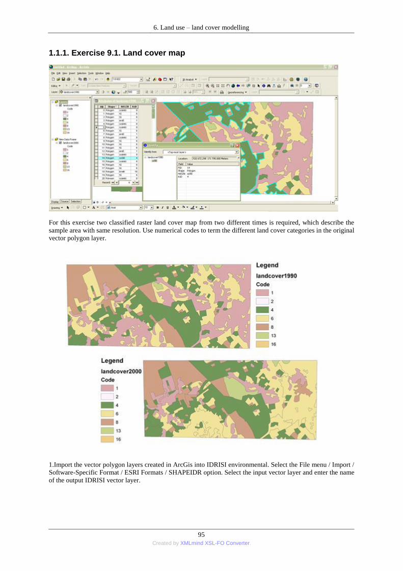
6. Land use – land cover modelling
95 Created by XMLmind XSL-FO Converter.
1.1.1. Exercise 9.1. Land cover map
For this exercise two classified raster land cover map from two different times is required, which describe the
sample area with same resolution. Use numerical codes to term the different land cover categories in the original
vector polygon layer.
1.Import the vector polygon layers created in ArcGis into IDRISI environmental. Select the File menu / Import /
Software-Specific Format / ESRI Formats / SHAPEIDR option. Select the input vector layer and enter the name
of the output IDRISI vector layer.
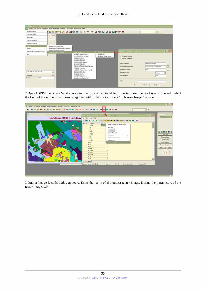
6. Land use – land cover modelling
96 Created by XMLmind XSL-FO Converter.
2.Open IDRISI Database Workshop window. The attribute table of the imported vector layer is opened. Select
the field of the numeric land use categories with right clicks. Select ―to Raster Image‖ option.
3.Output Image Details dialog appears. Enter the name of the output raster image. Define the parameters of the
raster image. OK.

6. Land use – land cover modelling
97 Created by XMLmind XSL-FO Converter.
4.Repeat the above mentioned process again to import the second vector layer.
1.1.2. Exercise 9.2. The evaluation of gains, losses and net change
5.Define the Working Folder, which contains the two land cover maps. Open IDRISI Explorer, click on the
Project tab, right-click with mouse and select the New Project option.
6.Open the LCM modeller from the Modeling menu / Environmental / Simulations Model menu.

6. Land use – land cover modelling
98 Created by XMLmind XSL-FO Converter.
7.In the LCM Project Parameters panel click on the Create new project button and enter the name. Select the
earlier and later land cover images. Optionally, you can select elevation layer, or palette file. Click the Continue
button.

6. Land use – land cover modelling
99 Created by XMLmind XSL-FO Converter.
8.Under the Change Map box, select the Map changes option to create map from net changes, enter the output
file name, if you keep the result and click the Create Map button.
9.Under the Change Map box, select the Map gains / losses in option, and select the category having the biggest
changes from drop-down list to create map. Enter the output file name, if you keep the result.
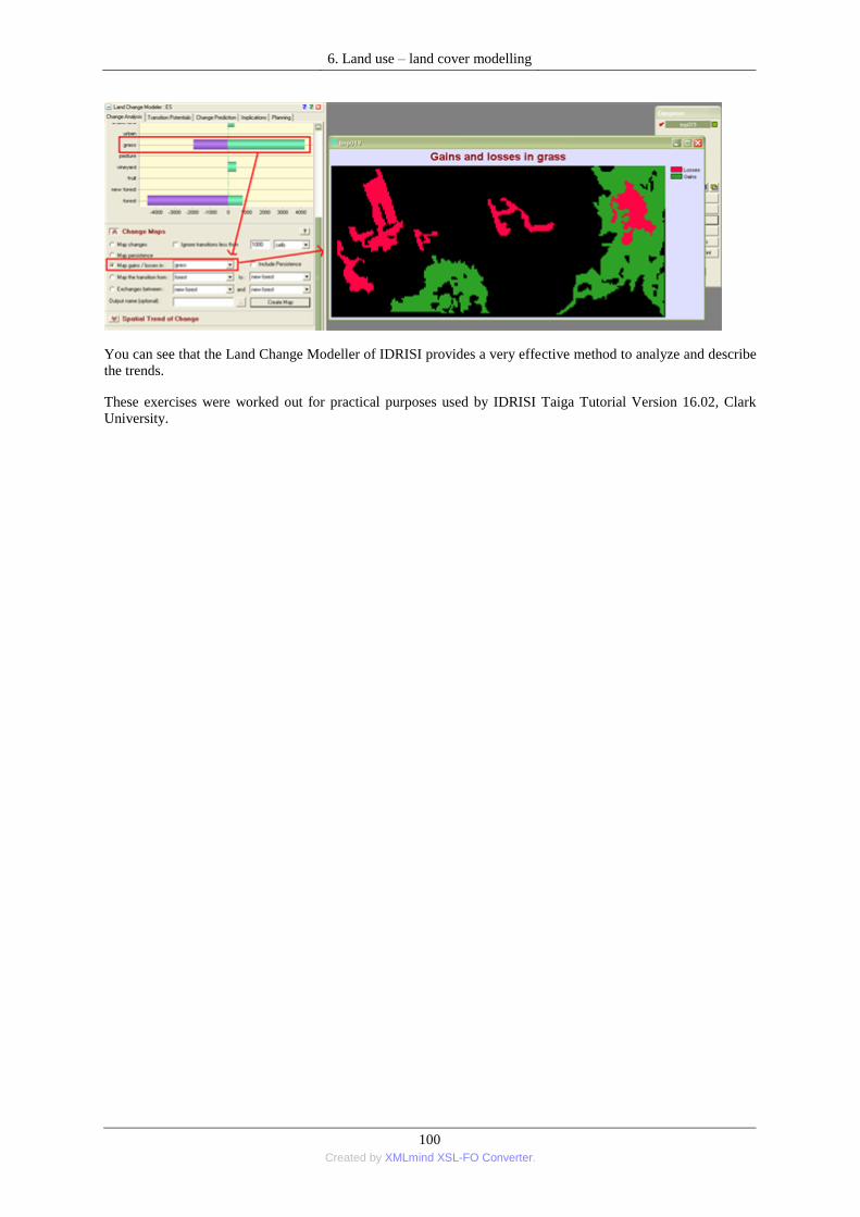
6. Land use – land cover modelling
100 Created by XMLmind XSL-FO Converter.
You can see that the Land Change Modeller of IDRISI provides a very effective method to analyze and describe
the trends.
These exercises were worked out for practical purposes used by IDRISI Taiga Tutorial Version 16.02, Clark
University.

101 Created by XMLmind XSL-FO Converter.
7. fejezet - 7. Environmental modelling
1.
The environmental model is a representation of numerous processes that are believed to occur on the Earth‘s
surface. It is a computer application that takes a digital representation of one or more aspects of the real world
and transforms then to create a new demonstration (Maguire et al., 2005).
However, one phenomenon can be described as the variation of spatial data over the Earth‘s surface. A high-
resolution DEM, soil map, vegetation map can also be used as input for modeling landscape development,
planning and recultivation.
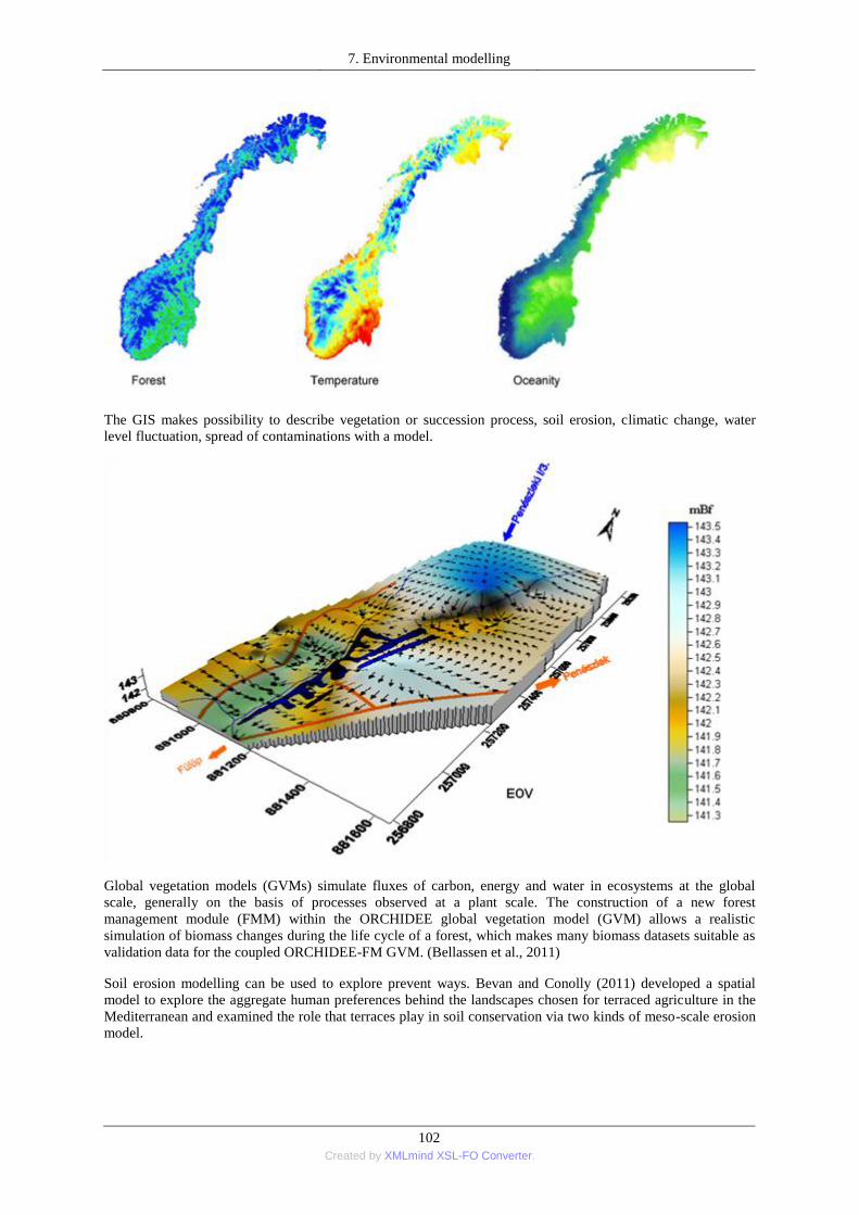
7. Environmental modelling
102 Created by XMLmind XSL-FO Converter.
The GIS makes possibility to describe vegetation or succession process, soil erosion, climatic change, water
level fluctuation, spread of contaminations with a model.
Global vegetation models (GVMs) simulate fluxes of carbon, energy and water in ecosystems at the global
scale, generally on the basis of processes observed at a plant scale. The construction of a new forest
management module (FMM) within the ORCHIDEE global vegetation model (GVM) allows a realistic
simulation of biomass changes during the life cycle of a forest, which makes many biomass datasets suitable as
validation data for the coupled ORCHIDEE-FM GVM. (Bellassen et al., 2011)
Soil erosion modelling can be used to explore prevent ways. Bevan and Conolly (2011) developed a spatial
model to explore the aggregate human preferences behind the landscapes chosen for terraced agriculture in the
Mediterranean and examined the role that terraces play in soil conservation via two kinds of meso-scale erosion
model.

7. Environmental modelling
103 Created by XMLmind XSL-FO Converter.
The spread of invasive species is also the one of the major ecological and economic problem. Pitt et al. (2011)
examined the spatial distribution of B. davidii through time and space in Europe, and tried to apply successfully
these parameters to a model of the spread of the species in New Zealand.
The cause and effect of natural or ecosystem risks can be integrate the combination of natural and human-
induced stressors that constitute environmental risk and risk assessment. Romeiro et al., (2011) simulated the
transport of pollutants at Igapó I Lake, located in Londrina, Paraná, Brazil.

7. Environmental modelling
104 Created by XMLmind XSL-FO Converter.
2. 7.1. GIS functions
GIS basic functions aimed at interaction among layers. The GIS can perform a spatial analysis; spatial
relationships among the features and their attributes and the persistent link with their geometry (shape and
position) make the GIS a tool able to simulate the real world and hence to help decision makers in solving actual
problems and in forecasting potential consequences of risky phenomena. Operations can be carried out on a
single data layer or by combining two or more data layers. Spatial interpolation, for example, is the most
common task performed on a single layer. (Gomarasca, 2009)
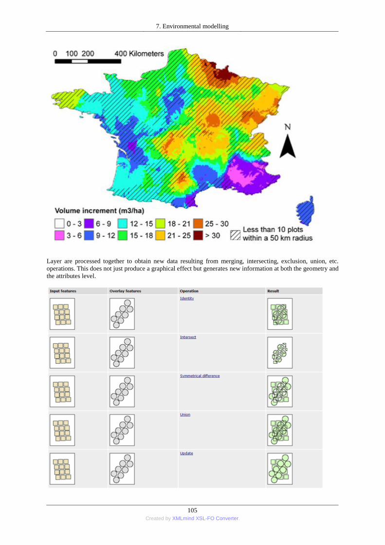
7. Environmental modelling
105 Created by XMLmind XSL-FO Converter.
Layer are processed together to obtain new data resulting from merging, intersecting, exclusion, union, etc.
operations. This does not just produce a graphical effect but generates new information at both the geometry and
the attributes level.

7. Environmental modelling
106 Created by XMLmind XSL-FO Converter.
Neighbourhood tools: useful to evaluate the behaviour of portions of maps near a specific position. It performs
the computation of distances between two or more elements. The distance has to be intended as a generic cost
function, in which many conditioning factors are involved. Typical examples are the determination of buffering
zones around critical features, or the generation of the Thiessen polygons. The GIS capability to create variable
and asymmetric buffering zones according to the reference mapped features can solve complex problems and
produce new thematic layers useful for decision makers.
A buffer zone is any area that serves the purpose of keeping real world features distant from one another. Buffer
zones are often set up to protect the environment, protect residential and commercial zones from industrial
accidents or natural disasters, or to prevent violence. (Sutton et al., 2009)
Topographic (surface or Spatial Analyst) functions: permit the calculation and mapping slope, aspect, viewshed
of a certain space-dependent function (grid format). These operations are typical of the raster model.
Solar radiation tools: aimed at calculating the parameters related to the incoming sun radiation, hence
determining how many hours a certain side of a mountain, or of a building, is exposed to the Sun.

7. Environmental modelling
107 Created by XMLmind XSL-FO Converter.
Interpolation tools: They calculate new values of the functions in new positions lying between the original
widely spaced ones. Original point (or line) distribution can be either regular or irregular.
Connectivity (topology) tools: They are useful to identify if and how segments of a network (of polygons or
lines) are connected. The main ones are contiguity functions: consider those areas having common properties
and evaluate the characteristics of the connected features among them. For example, to identify a suitable
candidate area (sum of different polygons) as a natural reserve within a certain region, contiguity rules could be
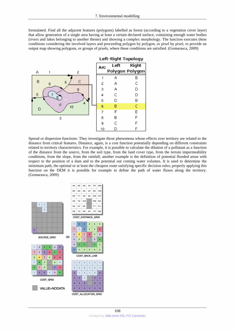
7. Environmental modelling
108 Created by XMLmind XSL-FO Converter.
formulated. Find all the adjacent features (polygons) labelled as forest (according to a vegetation cover layer)
that allow generation of a single area having at least a certain declared surface, containing enough water bodies
(rivers and lakes belonging to another theme) and showing a complex morphology. The function executes these
conditions considering the involved layers and proceeding polygon by polygon, or pixel by pixel, to provide an
output map showing polygons, or groups of pixels, where these conditions are satisfied. (Gomarasca, 2009)
Spread or dispersion functions: They investigate those phenomena whose effects over territory are related to the
distance from critical features. Distance, again, is a cost function potentially depending on different constraints
related to territory characteristics. For example, it is possible to calculate the dilution of a pollutant as a function
of the distance from the source, from the soil type, from the land cover type, from the terrain impermeability
conditions, from the slope, from the rainfall; another example is the definition of potential flooded areas with
respect to the position of a dam and to the potential out coming water volumes. It is used to determine the
minimum path, the optimal or at least the cheapest route satisfying specific decision rules; properly applying this
function on the DEM it is possible for example to define the path of water fluxes along the territory.
(Gomarasca, 2009)
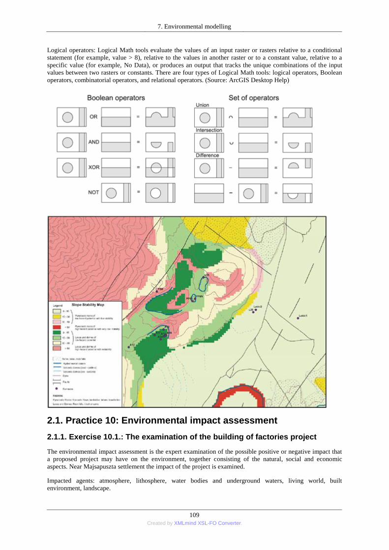
7. Environmental modelling
109 Created by XMLmind XSL-FO Converter.
Logical operators: Logical Math tools evaluate the values of an input raster or rasters relative to a conditional
statement (for example, value > 8), relative to the values in another raster or to a constant value, relative to a
specific value (for example, No Data), or produces an output that tracks the unique combinations of the input
values between two rasters or constants. There are four types of Logical Math tools: logical operators, Boolean
operators, combinatorial operators, and relational operators. (Source: ArcGIS Desktop Help)
2.1. Practice 10: Environmental impact assessment
2.1.1. Exercise 10.1.: The examination of the building of factories project
The environmental impact assessment is the expert examination of the possible positive or negative impact that
a proposed project may have on the environment, together consisting of the natural, social and economic
aspects. Near Majsapuszta settlement the impact of the project is examined.
Impacted agents: atmosphere, lithosphere, water bodies and underground waters, living world, built
environment, landscape.

7. Environmental modelling
110 Created by XMLmind XSL-FO Converter.
1.On the basis of the topographic map with 1:25000 resolution the main mine sites, waste disposals, wastewater
settling poles, industrial railways and building estates; as well as natural and built features (e.g.: lake, river,
settlement) have to be digitalized.
2.Create 150 meters wide buffer zones around the mine sites, industrial railways and the avenues the way there.

7. Environmental modelling
111 Created by XMLmind XSL-FO Converter.
Open the ArcToolbox / Analysis Tools / Proximity / Buffer tool. Enter the input and the output file name, and
define the Linear unit of the buffer zone.
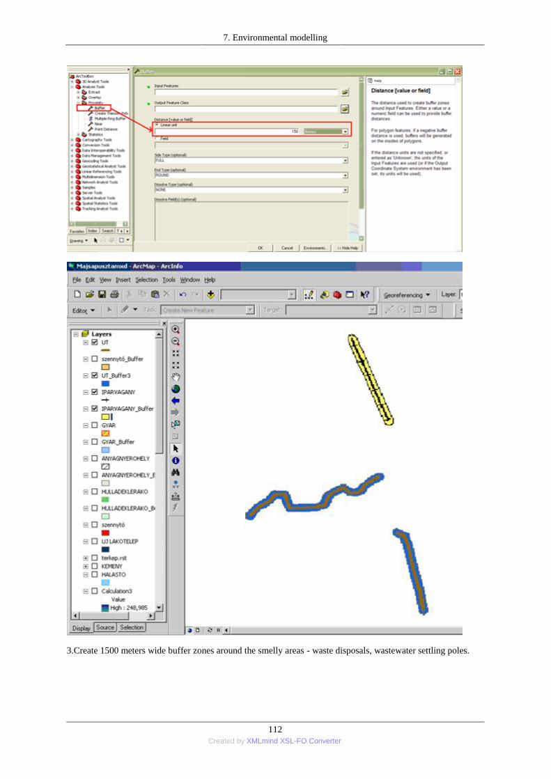
7. Environmental modelling
112 Created by XMLmind XSL-FO Converter.
3.Create 1500 meters wide buffer zones around the smelly areas - waste disposals, wastewater settling poles.

7. Environmental modelling
113 Created by XMLmind XSL-FO Converter.
4.Then combine the different buffer zones with the ArcToolbox / Analysis Tools / Overlay / Union tool.

7. Environmental modelling
114 Created by XMLmind XSL-FO Converter.
5.These operations can be performed with the help of the Model Builder. Model Builder is an application in
which you create, edit, and manage models. Open ArcToolbox window, and create a new toolbox. Name this
toolbox to Buffer exercise. Create a new model, right-click the Buffer exercise toolbox and click New Model.
The Model Builder window will open and the diagram area will be empty.
6.Next, locate the Buffer tool in the ArcToolbox window. Drag and drop the Buffer tool onto the Model Builder
diagram. Double-click the Buffer tool to open its dialog (or right-click and click Open). You only need to
provide the required parameters.

7. Environmental modelling
115 Created by XMLmind XSL-FO Converter.
7.The model should now appear. The blue oval represents input data, and the green oval represents output data.
You can resize the oval by clicking it to show its blue resize handles. Click and hold a resize handle and drag
your mouse to resize. If you click in the centre of the oval and drag the mouse, you can reposition the oval
anywhere on the Model Builder diagram area. Do the above mentioned steps again to create complete model.
The model is now ready to run. You can run the model from the Model Builder window by clicking the Run
button.
8.Do the above mentioned steps again to create impact areas of the different agent with the appropriate extent.

7. Environmental modelling
116 Created by XMLmind XSL-FO Converter.
9.Combine the impact area of the different agents with the ArcToolbox / Analysis Tools / Overlay / Union tool.
These operations can be performed with the help of the Model Builder.
These exercises were worked out for practical purposes used by ESRI Desktop Online Help.
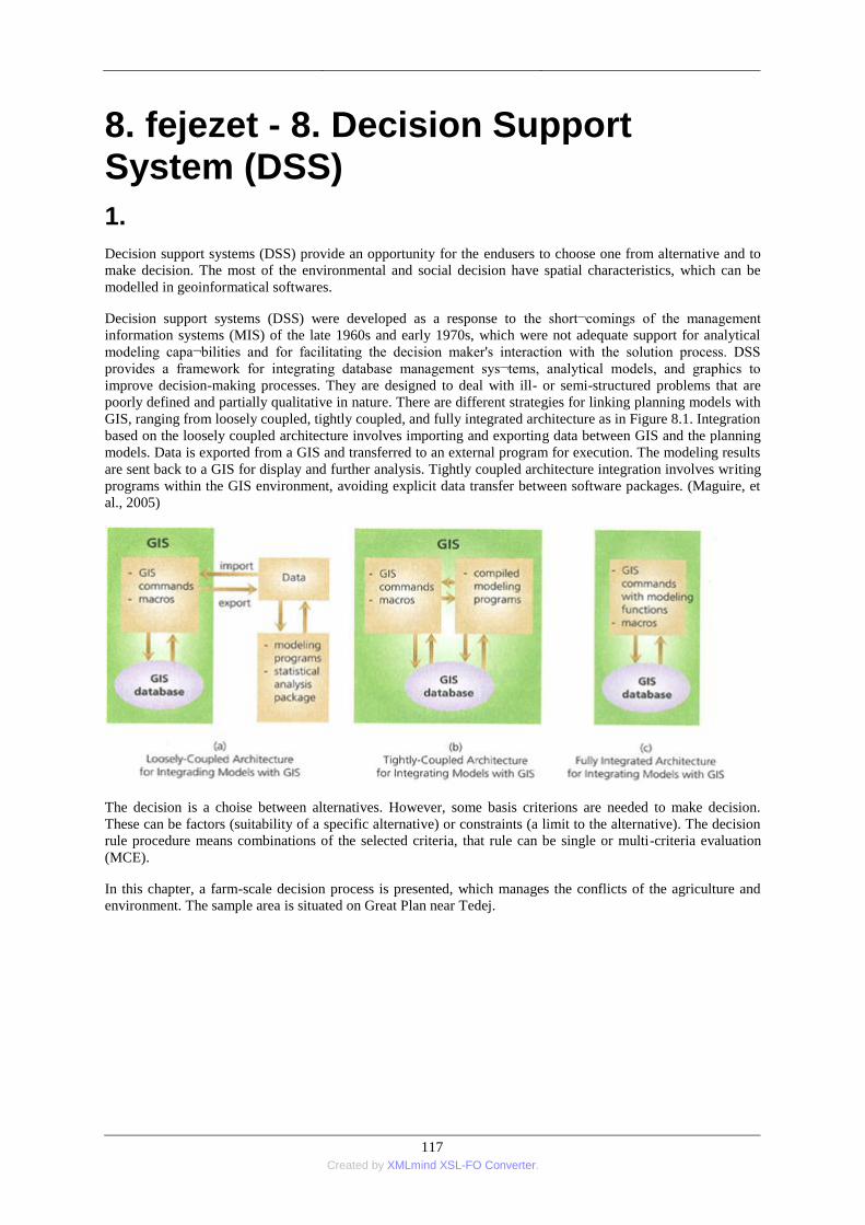
117 Created by XMLmind XSL-FO Converter.
8. fejezet - 8. Decision Support System (DSS)
1.
Decision support systems (DSS) provide an opportunity for the endusers to choose one from alternative and to
make decision. The most of the environmental and social decision have spatial characteristics, which can be
modelled in geoinformatical softwares.
Decision support systems (DSS) were developed as a response to the short¬comings of the management
information systems (MIS) of the late 1960s and early 1970s, which were not adequate support for analytical
modeling capa¬bilities and for facilitating the decision maker's interaction with the solution process. DSS
provides a framework for integrating database management sys¬tems, analytical models, and graphics to
improve decision-making processes. They are designed to deal with ill- or semi-structured problems that are
poorly defined and partially qualitative in nature. There are different strategies for linking planning models with
GIS, ranging from loosely coupled, tightly coupled, and fully integrated architecture as in Figure 8.1. Integration
based on the loosely coupled architecture involves importing and exporting data between GIS and the planning
models. Data is exported from a GIS and transferred to an external program for execution. The modeling results
are sent back to a GIS for display and further analysis. Tightly coupled architecture integration involves writing
programs within the GIS environment, avoiding explicit data transfer between software packages. (Maguire, et
al., 2005)
The decision is a choise between alternatives. However, some basis criterions are needed to make decision.
These can be factors (suitability of a specific alternative) or constraints (a limit to the alternative). The decision
rule procedure means combinations of the selected criteria, that rule can be single or multi-criteria evaluation
(MCE).
In this chapter, a farm-scale decision process is presented, which manages the conflicts of the agriculture and
environment. The sample area is situated on Great Plan near Tedej.
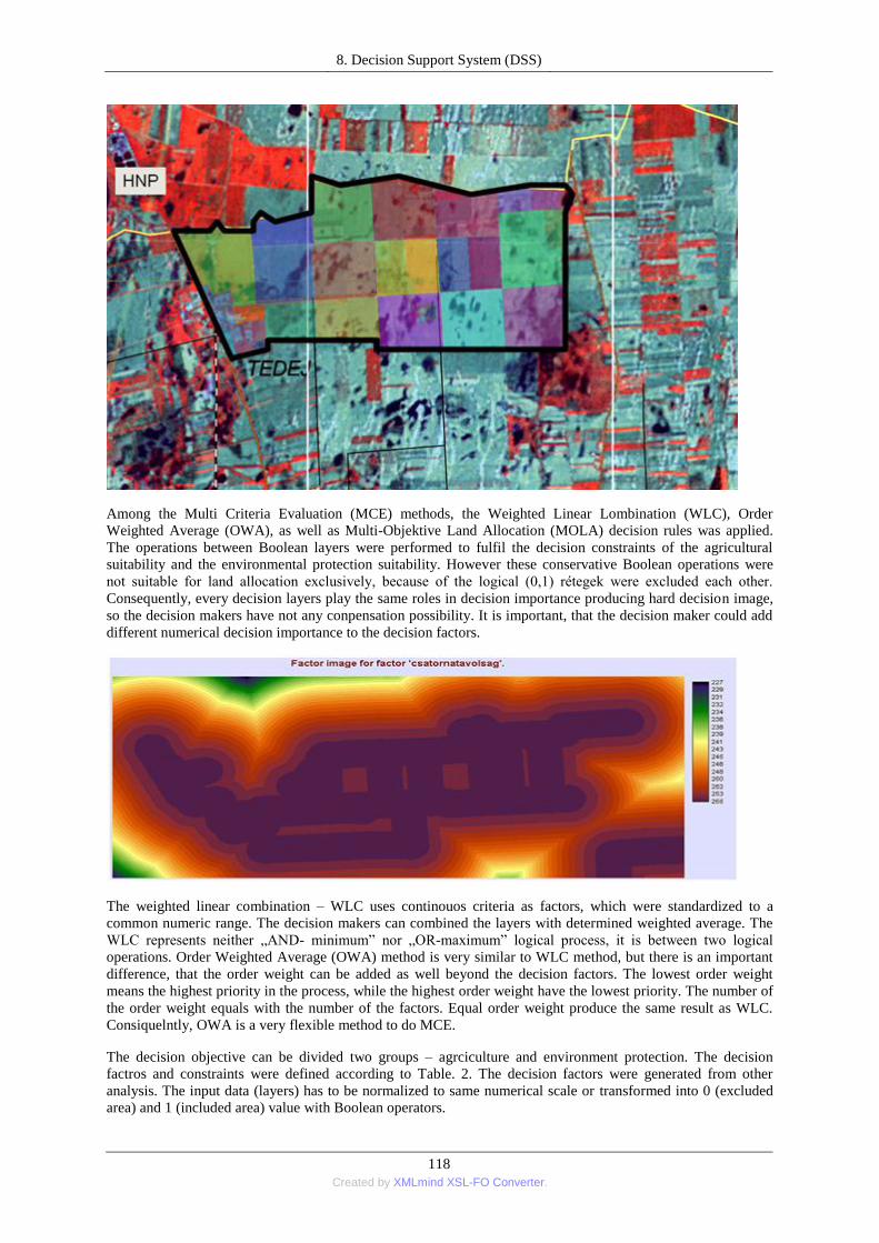
8. Decision Support System (DSS)
118 Created by XMLmind XSL-FO Converter.
Among the Multi Criteria Evaluation (MCE) methods, the Weighted Linear Lombination (WLC), Order
Weighted Average (OWA), as well as Multi-Objektive Land Allocation (MOLA) decision rules was applied.
The operations between Boolean layers were performed to fulfil the decision constraints of the agricultural
suitability and the environmental protection suitability. However these conservative Boolean operations were
not suitable for land allocation exclusively, because of the logical (0,1) rétegek were excluded each other.
Consequently, every decision layers play the same roles in decision importance producing hard decision image,
so the decision makers have not any conpensation possibility. It is important, that the decision maker could add
different numerical decision importance to the decision factors.
The weighted linear combination – WLC uses continouos criteria as factors, which were standardized to a
common numeric range. The decision makers can combined the layers with determined weighted average. The
WLC represents neither „AND- minimum‖ nor „OR-maximum‖ logical process, it is between two logical
operations. Order Weighted Average (OWA) method is very similar to WLC method, but there is an important
difference, that the order weight can be added as well beyond the decision factors. The lowest order weight
means the highest priority in the process, while the highest order weight have the lowest priority. The number of
the order weight equals with the number of the factors. Equal order weight produce the same result as WLC.
Consiquelntly, OWA is a very flexible method to do MCE.
The decision objective can be divided two groups – agrciculture and environment protection. The decision
factros and constraints were defined according to Table. 2. The decision factors were generated from other
analysis. The input data (layers) has to be normalized to same numerical scale or transformed into 0 (excluded
area) and 1 (included area) value with Boolean operators.

8. Decision Support System (DSS)
119 Created by XMLmind XSL-FO Converter.
In case of vector input layers the Boolean operations can be used, while WLC operations are suitable device in
raster system to do MCE generally.
In IDRISI the Multi-Objective Land Allocation (MOLA) module is designed to allocate locations based upon
total area thresholds and to resolve areas where multiple objectives conflict. MOLA requires the name of the
objectives, the relative weight to assign to each, and the area to be alloced to each. (IDRISI Taiga Tutorial)

8. Decision Support System (DSS)
120 Created by XMLmind XSL-FO Converter.

121 Created by XMLmind XSL-FO Converter.
9. fejezet - References
1.
• Aitkenhead, M.J. and Aalders, I.H. (2011): Automating land cover mapping of Scotland using expert system
and knowledge integration methods. Remote Sensing of Environment, No. 115, 1285–1295pp.
• Bellassen, V., le Maire,G., Guin,O., Dhôte, J.F., Ciais,P., Viovy N. (2011): Modelling forest management
within a global vegetation model—Part 2: Model validation from a tree to a continental scale. Ecological
Modelling, No. 222, 57–75pp.
• Bernhardsen, T. (1992): Geographic Information System. Viak IT, Norway
• Bevan, A., Conolly, J. (2011): Terraced fields and Mediterranean landscape structure: An analytical case
study from Antikythera, Greece. Ecological Modelling, No. 222, 1303–1314pp.
• Bozán, Cs., Tamás, J. (2010): Applied land change modelling based on excess water affected areas for agro-
ecological sustainability on the southern great plain. 9th Alps-Adria Scientific Workshop, Špičák, Czech
Republic, 191-194 pp.
• Burai, P, Tamás, J. (2004): Hyper- and multispectral remote sensing technologies in precisional agricultural
water management. In: Proc. III. Alps-Adria Scientific Workshop, (Dubrovnik, Croatia) 54–57.
• Burai, P., Kovács, E., Lénárt, Cs., Nagy, A., Nagy, I. (2009): Quantification of vegetation stress based on
hyperspectral image processing. Cereal Research Communications. Akadémiai Kiadó. Budapest. 37. pp. 581-
584.
• Campbell, J. B. (2002): Introduction to remote sensing. Taylor and Francis, London
• Casalí, J., Giménez, R., De Santisteban, L., Álvarez-Mozos, J., Mena, J., Del Valle de Lersundi J. (2009):
Determination of long-term erosion rates in vineyards of Navarre (Spain) using botanical benchmarks.
Catena, No. 78, 12–19 pp.
• Chio, S. (2008): A study on roof point extraction based on robust estimation from airborne lidar data. Journal
of the Chinese Institute of Engineers, Vol. 31, No. 4, 537-550 pp.
• Christopherson, R.W., (1994): An Introduction to Physical Geography, 2nd GEOSYSTEMS Ed. ©. Prentice
Hall
• Crackneel, A. and Hayes L. (1993): Introduction to Remote Sensing, Taylor and Francis, London
• Dalyot, S. and Doytsher, Y. (2009): Hierarchical Modelling of Multi-Geospatial Databases as Basis for Geo-
Oriented 3D Analysis Capabilities In: Lee, Jiyeong – Zlatanova, Sisi (Eds.): 3D Geo-Information Sciences.
Springer-Verlag, Berlin, Heidelberg
• De Lara, R. Jr. - Mitishita, E. A. – Vögtle, T. – Bähr, H. P. (2009): Automatic Digital Aerial Image Resection
Controlled by LIDAR Data In: Lee, Jiyeong – Zlatanova, Sisi (Eds.): 3D Geo-Information Sciences.
Springer-Verlag, Berlin, Heidelberg
• De Rienzo, F., Oreste, P., Pelizza, S. (2008): Subsurface geological-geotechnical modelling to sustain
underground civil planning. Engineering Geology, No. 96, 187–204 pp.
• Dezso, Zs., Bartholy, J., Pongracz, R., Barcza, Z. (2005): Analysis of land-use/land-cover change in the
Carpathian region based on remote sensing techniques. Physics and Chemistry of the Earth, No. 30, 109–
115pp.
• Dong, P. (2009): Lacunarity analysis of raster datasets and 1D, 2D, and 3D point patterns. Computers and
Geosciences, No. 35, 2100–2110 pp.
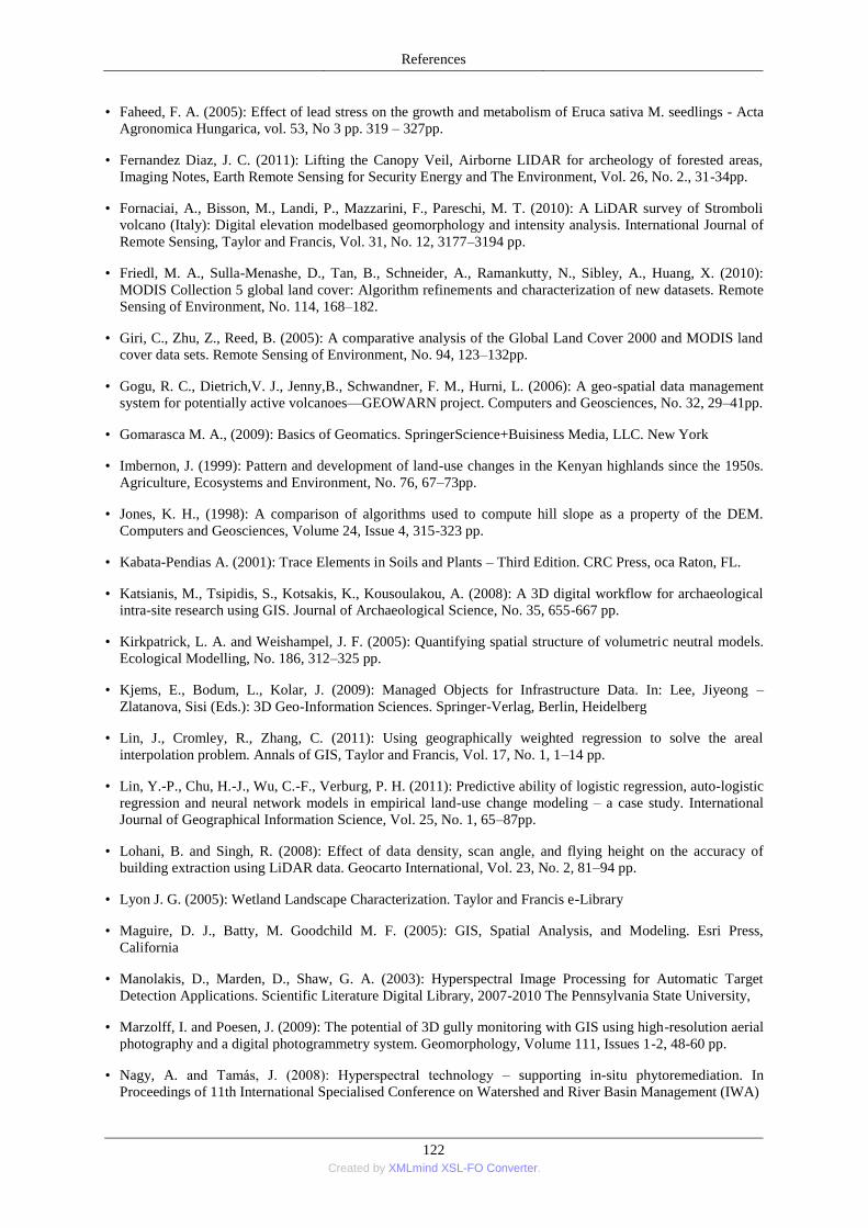
References
122 Created by XMLmind XSL-FO Converter.
• Faheed, F. A. (2005): Effect of lead stress on the growth and metabolism of Eruca sativa M. seedlings - Acta
Agronomica Hungarica, vol. 53, No 3 pp. 319 – 327pp.
• Fernandez Diaz, J. C. (2011): Lifting the Canopy Veil, Airborne LIDAR for archeology of forested areas,
Imaging Notes, Earth Remote Sensing for Security Energy and The Environment, Vol. 26, No. 2., 31-34pp.
• Fornaciai, A., Bisson, M., Landi, P., Mazzarini, F., Pareschi, M. T. (2010): A LiDAR survey of Stromboli
volcano (Italy): Digital elevation modelbased geomorphology and intensity analysis. International Journal of
Remote Sensing, Taylor and Francis, Vol. 31, No. 12, 3177–3194 pp.
• Friedl, M. A., Sulla-Menashe, D., Tan, B., Schneider, A., Ramankutty, N., Sibley, A., Huang, X. (2010):
MODIS Collection 5 global land cover: Algorithm refinements and characterization of new datasets. Remote
Sensing of Environment, No. 114, 168–182.
• Giri, C., Zhu, Z., Reed, B. (2005): A comparative analysis of the Global Land Cover 2000 and MODIS land
cover data sets. Remote Sensing of Environment, No. 94, 123–132pp.
• Gogu, R. C., Dietrich,V. J., Jenny,B., Schwandner, F. M., Hurni, L. (2006): A geo-spatial data management
system for potentially active volcanoes—GEOWARN project. Computers and Geosciences, No. 32, 29–41pp.
• Gomarasca M. A., (2009): Basics of Geomatics. SpringerScience+Buisiness Media, LLC. New York
• Imbernon, J. (1999): Pattern and development of land-use changes in the Kenyan highlands since the 1950s.
Agriculture, Ecosystems and Environment, No. 76, 67–73pp.
• Jones, K. H., (1998): A comparison of algorithms used to compute hill slope as a property of the DEM.
Computers and Geosciences, Volume 24, Issue 4, 315-323 pp.
• Kabata-Pendias A. (2001): Trace Elements in Soils and Plants – Third Edition. CRC Press, oca Raton, FL.
• Katsianis, M., Tsipidis, S., Kotsakis, K., Kousoulakou, A. (2008): A 3D digital workflow for archaeological
intra-site research using GIS. Journal of Archaeological Science, No. 35, 655-667 pp.
• Kirkpatrick, L. A. and Weishampel, J. F. (2005): Quantifying spatial structure of volumetric neutral models.
Ecological Modelling, No. 186, 312–325 pp.
• Kjems, E., Bodum, L., Kolar, J. (2009): Managed Objects for Infrastructure Data. In: Lee, Jiyeong –
Zlatanova, Sisi (Eds.): 3D Geo-Information Sciences. Springer-Verlag, Berlin, Heidelberg
• Lin, J., Cromley, R., Zhang, C. (2011): Using geographically weighted regression to solve the areal
interpolation problem. Annals of GIS, Taylor and Francis, Vol. 17, No. 1, 1–14 pp.
• Lin, Y.-P., Chu, H.-J., Wu, C.-F., Verburg, P. H. (2011): Predictive ability of logistic regression, auto-logistic
regression and neural network models in empirical land-use change modeling – a case study. International
Journal of Geographical Information Science, Vol. 25, No. 1, 65–87pp.
• Lohani, B. and Singh, R. (2008): Effect of data density, scan angle, and flying height on the accuracy of
building extraction using LiDAR data. Geocarto International, Vol. 23, No. 2, 81–94 pp.
• Lyon J. G. (2005): Wetland Landscape Characterization. Taylor and Francis e-Library
• Maguire, D. J., Batty, M. Goodchild M. F. (2005): GIS, Spatial Analysis, and Modeling. Esri Press,
California
• Manolakis, D., Marden, D., Shaw, G. A. (2003): Hyperspectral Image Processing for Automatic Target
Detection Applications. Scientific Literature Digital Library, 2007-2010 The Pennsylvania State University,
• Marzolff, I. and Poesen, J. (2009): The potential of 3D gully monitoring with GIS using high-resolution aerial
photography and a digital photogrammetry system. Geomorphology, Volume 111, Issues 1-2, 48-60 pp.
• Nagy, A. and Tamás, J. (2008): Hyperspectral technology – supporting in-situ phytoremediation. In
Proceedings of 11th International Specialised Conference on Watershed and River Basin Management (IWA)
References
123 Created by XMLmind XSL-FO Converter.
• Parrish, M. C. and Hepinstall-Cymerman, J., (2011): Using geospatial data and principles of landscape
ecology to identify field sites and characterize landscapes. Annals of GIS, Vol. 17, No. 1, 63–72 pp.
• Pavlopolous, K., Evelpidou, N., Vassilopoulos, A. (2009): Mapping Geomorphological Environments.
Springer-Verlag Berlin Heidelberg
• Pitt, J. P.W., Kriticos, D. J., Dodd, M. B. (2011): Temporal limits to simulating the future spread pattern of
invasive species: Buddleja davidii in Europe and New Zealand. Ecological Modelling, No. 222, 1880–
1887pp.
• Ritvayné, Sz. M., Frombach, G., Nagy, A. (2009): Remote sensing as a promising tool for environmental
assessment. Land Contamination and Reclaimation. 17 (3-4). 423-429.
• Rosell, J. R., Llorens, J., Sanz, R., Arnò, J., Ribes-Dasi, M., Masip, J., Escolà, A., Campc, F., Solanelles, F.,
Gràcia, F., Gil, E., Val, L., Planas, S., Palacìn, J. (2009): Obtaining the three-dimensional structure of tree
orchards from remote 2D terrestrial LIDAR scanning. Agricultural and Forest Meteorology, No. 149, 1505–
1515 pp.
• Serra, P., Pons, X., Saurı, D. (2008): Land-cover and land-use change in a Mediterranean landscape: A spatial
analysis of driving forces integrating biophysical and human factors. Applied Geography, Volume 28, Issue
3, 189-209pp.
• Shekhar, S., and Xiong, H. (2008): Encyclopedia of GIS. SpringerScience+Buisiness Media, LLC. New York
• Stokland, J. N., Halvorsen,R., Střa, B. (2011): Species distribution modelling—Effect of design and sample
size of pseudo-absence observations. Ecological Modelling, No. 222, 1800–1809pp.
• Suttom, T., Dassau, O., Sutton, M. (2009): A Gentle Introduction to GIS. Brought to you with Quantum GIS,
a Free and Open Source Software GIS Application for everyone, Spatial Planning and Information,
Department of Land Affairs, Eastern Cape
• Szucs, A., Jordan, G., Qvarfort, U. (2002). Geochemical modelling of acid mine drainage impact on wetland
stream using landscape geochemistry, GIS and statistical methods. In: Fabbri, A.G., Gaal, G., McCammon,
R.B.: Deposit and Geoenvironmental Models for Resource Exploitation an Environmental Security NATO
Science Series, 2. Environmental Security. Kluwer Academic Publishers 80, 425-460 pp.
• Stojic, M. and Sims, J. (2011): The New Paradigm. Imaging Notes, Earth Remote Sensing for Security
Energy and The Environment, Vol. 26, No. 2., 26-30pp.
• Tamás, J. (2003): Problems and solutions of field scale agro-ecological data acquisition and data
interpretations in agroinformatical domain. Applied Ecology and Enviromental Research, International
Scientific Journal, 1 (1-2). 143-159 pp.
• Tamás, J., Takács, P., Juhász, Cs. (2004): Integrated field scale water management technology. III. Alps-
Adria Scientific Workshop, Dubrovnik, Croatia, 112-117pp.
• Tamás, J. Lénárt, Cs. (2006): Analysis of small agricultural watershed using remote sensing techniques.
International Journal of Remote Sensing, Vol. 27. Number 17. Taylor and Francis. 3727-3738.pp.
• Tamás, J., Reisinge,r P., Burai, P., David, I. (2006): Geostatistical analysisi of spatial heterogenity of
Ambrosia artemisifolia on Hungarian acid sandy soil, Journal of Plant Diseases and Protection, Sonderheft,
Germany, 227-232 pp.
• Tamás, J., Lénárt, Cs., Burai, P. (2009): Evaluation of applicability of airborne AISA DUAL hyperspectral
imaging system to map environmental conditions in orchards. Internation Commission of Agricultural and
Biological Engineers, Section V. Conference ―Technology and Management to Increase the Efficiency in
Sustainable Agricultural Systems‖, Rosario, Argentina
• Tamás, J., Fórián, T., Nagy, A., Nyéki, J., Soltész, M. (2010): Pilot study for irrigation modelling of a pear
plantation. International Journal of Horticultural Science, Issue 16, No. 3, 81-85pp.

References
124 Created by XMLmind XSL-FO Converter.
• Weng, Q. (2010): Remote Sensing and GIS Integration, Theories, Methods, and Applications. The McGraw-
Hill Companies, Inc. eBook.
• Xian, G., Homer, C., Fry, J. (2009): Updating the 2001 National Land Cover Database land cover
classification to 2006 by using Landsat imagery change detection methods. Remote Sensing of Environment,
No. 113, 1133–1147pp.
• Yan, G., Bradshaw, A.D. (1995): The containment of toxic wastes: II. Metal movement in leachate and
drainage at Parc Lead-Zinc Mine, North Wales, Environmental Pollution, 90(3), 379-382 pp.
• Yu, B., Liu, H., Wu, J., Lin, W. (2009): Investigating impacts of urban morphology on spatio-temporal
variations of solar radiation with airborne LIDAR data and a solar flux model: a case study of downtown
Houston. International Journal of Remote Sensing, Vol. 30, No. 17, 4359–4385 pp.
• Zeilhofer, P., Schwenk, L. M., Onga N. (2011): A GIS-approach for determining permanent riparian
protection areas in Mato Grosso, central Brazil. Applied Geography, Volume 31, Issue 3, 990-997 pp.
• Zhou, B. (2007): Application of hyperspectral remote sensing in detecting and mapping sericea lespedeza in
Missouri. Thesis, The Faculty of the Graduate School University of Missouri-Columbia
2. Manuals, Tutorials
• Leica Geosystems (2006) ERDAS IMAGINE® Tour Guides™. Leica Geosystems Geospatial Imaging, LLC,
Atlanta.
• ESRI Technical Description (2006) Environmental Systems Research Institute, Inc., Redlands, USA.,
• ENVI Version 4.7 (2009) Copyright © ITT Visual Information Solutions
• IDRISI Taiga Tutorial Version 16.02, Clark University
• Surfer® Quick Start Guide Contouring and 3D Surface Mapping for Scientists and Engineers
• eCognition Professional 4.0 User Guide
• IDRISI Taiga Tutorial
• Internet
• http://en.wikipedia.org/wiki/Multi-spectral_image
• http://landsat.gsfc.nasa.gov
• European Environmental Agency, CORINE Land Cover Project, CORINE land cover technical guide –
Addendum 2000. http://www.eea.europa.eu/publications/COR0-landcover
• http://fomi.hu
• http://www.glcn.org
• http://www.esri.com/
• http://www.goldensoftware.com

125 Created by XMLmind XSL-FO Converter.
10. fejezet - Appendix
1.

Appendix
126 Created by XMLmind XSL-FO Converter.
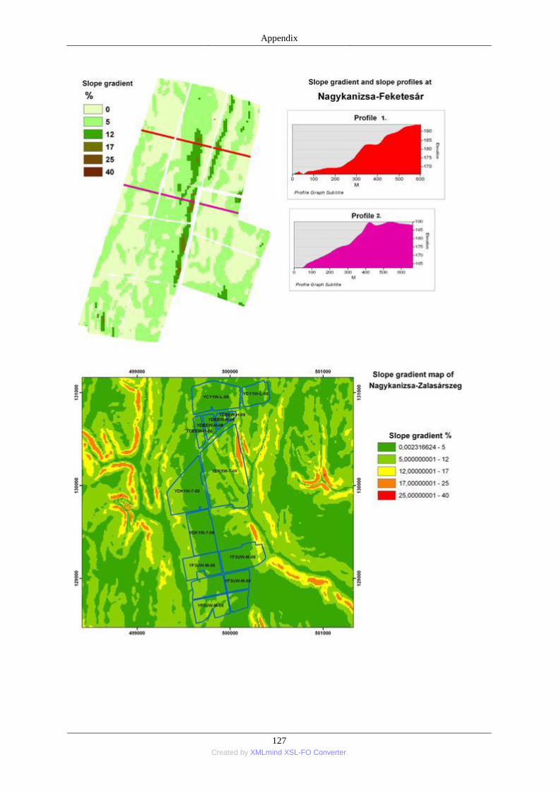
Appendix
127 Created by XMLmind XSL-FO Converter.
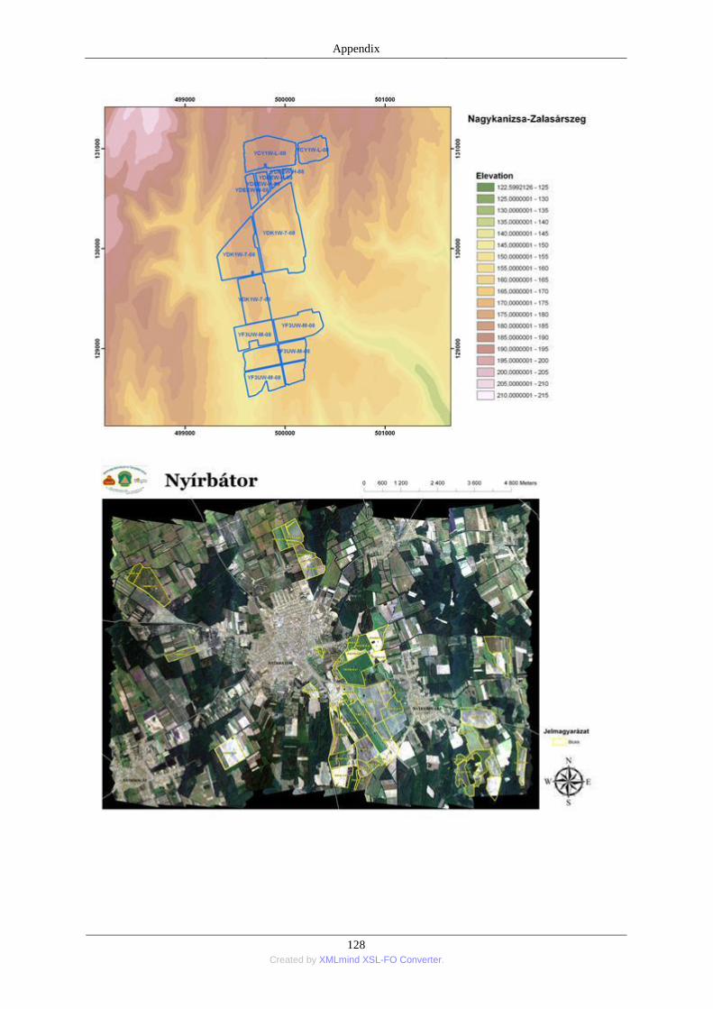
Appendix
128 Created by XMLmind XSL-FO Converter.
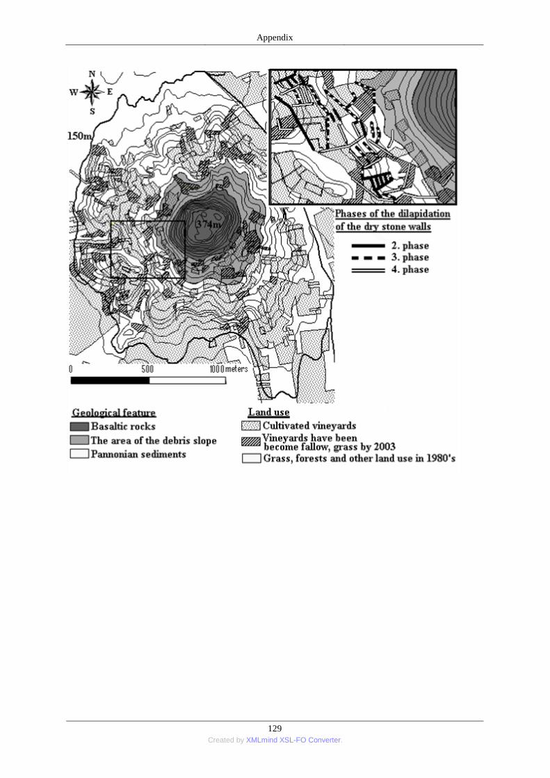
Appendix
129 Created by XMLmind XSL-FO Converter.

Appendix
130 Created by XMLmind XSL-FO Converter.

Appendix
131 Created by XMLmind XSL-FO Converter.
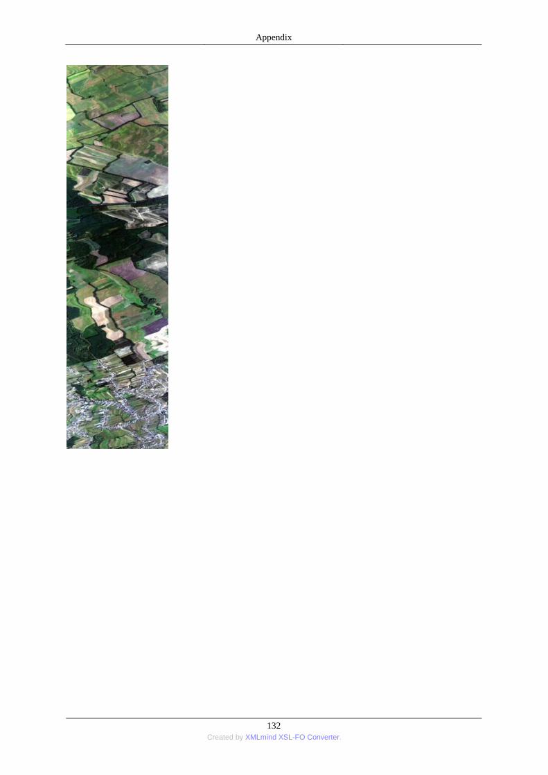
Appendix
132 Created by XMLmind XSL-FO Converter.
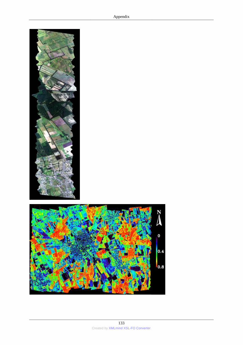
Appendix
133 Created by XMLmind XSL-FO Converter.
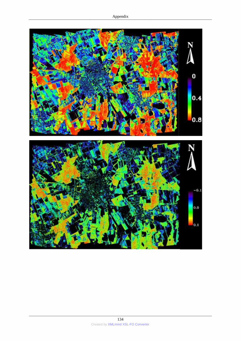
Appendix
134 Created by XMLmind XSL-FO Converter.