GENETIC POPULATION STRUcrURE OF CHINOOK SALMON,ONCORHYNCHUS TSHAWYTSCHA, IN THE PACIFIC NORTHWEST

F. UTTER,! G. MILNER,! G. STKHL,2 AND D. '!'EEL!

ABSTRACf

Variation at 25 polymorphic protein coding loci was examined for 86 populations of chinook salmon,Oncorhynd&1Ul tshau,ylscha, ranging from the Babine River in British Columbia to the Sacramento Riverin California. Substantial differences in allele frequencies identified patterns of genetic variability overthe geographic range of the study. The following nine major genetically defined regions were fonnu­lated: 1) the Fraser River tributaries east of the Cascade Crest (no downstream drainages were sam­pled), 2) Georgia Strait, 3) Puget Sound, 4) a broad coastal region ranging from the west coast of VancouverIsland southward through northern California, 5) the Columbia River below The Dalles Dam. 6) theColumbia River above The Dalles Dam, 7) the Snake River, 8) the K1antath River, and 9) the SacrantentoRiver. Populations sampled within a region tended to be genetically distinct from each other althoughthey exhibited the general patterns of variability that defined the region. Within a region there was littledistinction among populations returning to spawn at different times. The persistence of these geographicpatterns in the face of natural opportunities for introgression, and sometimes massive transplantations,suggests that genetically adapted groups within regions have resisted large-scale introgression from otherregions. Repopulation of deglaciated areas in the Frasl'r River, Georgia Strait, and Puget Sound ap­parently occurred from multiple sources; most likely sources included Columbia River populations andnorthern refuges rather than from the large coastal group of populations. Patterns of genetic distribu­tion of chinook salmon differed from those of other anadromous salmonids studied within this region.A conservative policy for stock transfers was suggested based on distinct genetic differences observedboth between and within regions.

Population studies of chinook salmon, Oncorkynck1t8t.shau'Ytscha, based on electrophoretically detectedgenetic variation have been carried out since the late1960s. As data have accumulated, an increasinglyclear picture of the breeding structure of this specieshas emerged. While early investigations based ononly a few polymorphic loci identified differencesamong populations, they failed to identify any geo­graphic trends (e.g., Utter et al. 1973; Kristianssonand McIntyre 1976). Differences within and amongdrainages became apparent as additional polymor­phic loci were found and a more comprehensivesampling of populations was made (Utter et al. 1976,1980; Gharrett et al. 1987).

This paper outlines the genetic structure ofchinook salmon in the Pacific Northwest using allelefrequency data collected for the purpose of esti­mating the stock composition of ocean caughtchinook salmon (Milner et al. 19813; 1983'; Miller

'Coastal Zone and Estuarine Studies Division, Northwest andAlaska Fisheries Center, National Marine Fisheries Service,NOAA, 2725 Montlake Boulevard East, Seattle, WA 98112.

sDepartmentofGenetics, Stockholm University, S-10691, Stock­holm, Sweden.

"Milner, G. B., D. J. Teel, F. M. Utter, and C. L. Burley. 1981.Columbia River stock identification study: Validation of genetic

Manuscript accepted January 1989.Fishery Bulletin, U.S. 87:239-264.

et al. 1983; Utter et a1. 1987). Our purpose is to ex­amine these data in the light of other relevant bio­logical and historical information 1) to understandgenetic relationships among chinook salmon popu­lations better and 2) to provide biologists with newinsights to assist in the preservation and manage­ment of this important biological resource.

MATERIALS AND METHODS

Our data were obtained from samples of juvenileor adult fish collected at 86 locations ranging fromBritish Columbia through California (Table I, Fig.1). These data include allele frequencies from 25protein-coding loci with sample sizes between 38 and200 individuals. Data were accumulated between1980 and 1984 and were reported in part in Milneret a1. (fn. 3, 4).

Electrophoretic procedures followed those de-

method. Report to Bonneville Power Administration under con­tract DE-AI79-80BPI8488, 51 p. Available Bonneville Power Ad­ministration, P.O. Box 3621, Portland, OR 97208.

<Milner, G. B., D. J. Teel, and F. M. Utter. 1983. Genetic stockidentification study. Report to Bonneville Power Administrationunder contract DE-AI79-82BP28044M001, 95 p. Available Bonne­ville Power Administration, P.O. Box 3621, Portland, OR 97208.

239

FISHERY BULLETIN: VOL. 87, NO.2. 1989

1000km

1

2

3

CANADA

M u.s.

240

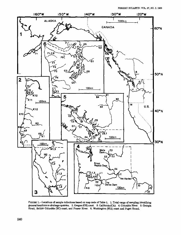
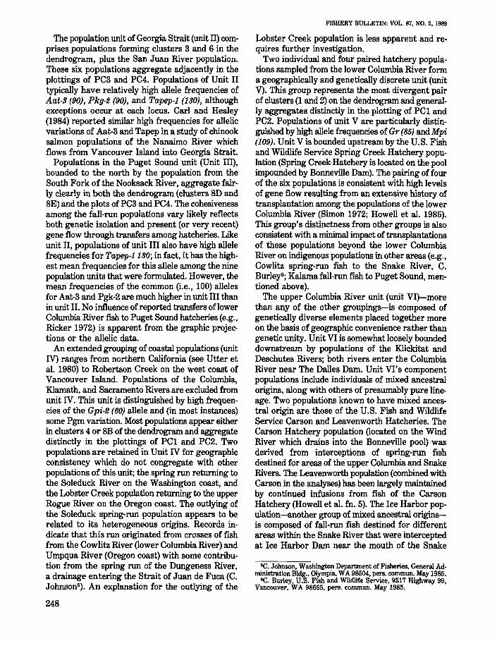
FIGURE I.-Locations of sample collections based on map code of Table 1. 1. Total range of sampling identifyinggeneral locations or drainage systems. 2. Oregon (OR) coast. 3. California (CA). 4. Columbia River. 5. GeorgiaStrait, British Columbia (BC) coast, and Fraser River. 6. Washington (WA) coast and puget Sound.

UTTER ET AL.: GENETIC POPULATION STRUCTURE OF CHINOOK SALMON

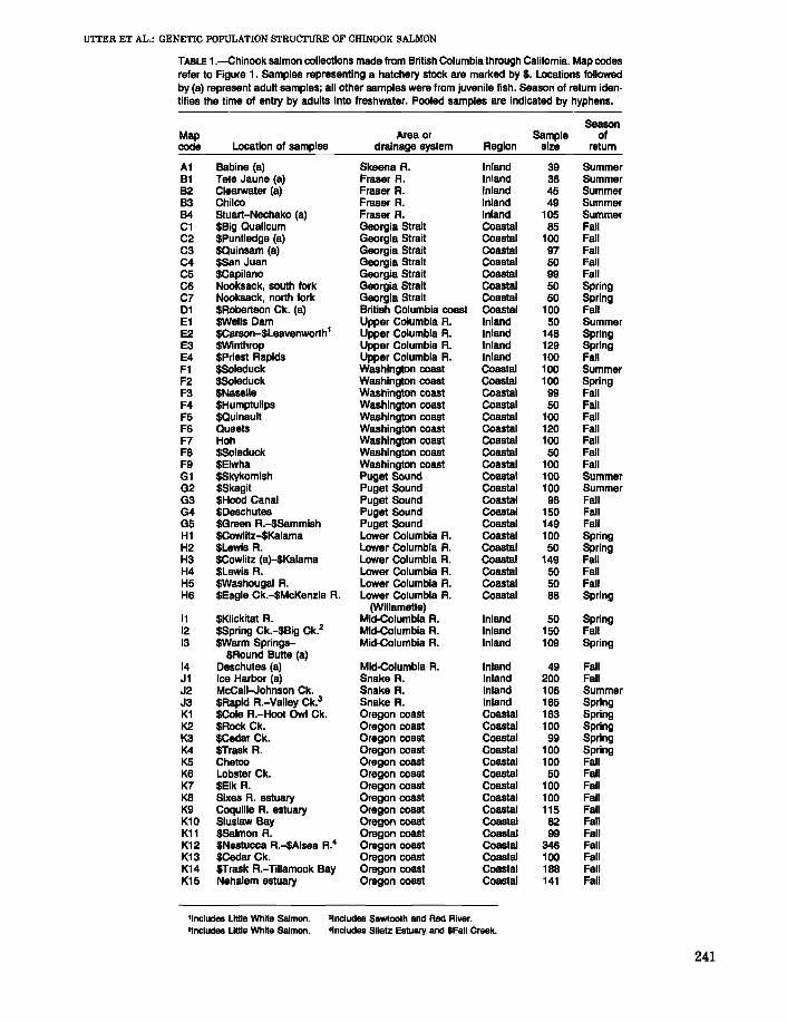
TABLE 1.-Chinook salmon collections made from British Columbia through California. Map codesrefer to Figure 1. Samples representing a hatchery stock are marked by $. Locations followedby (a) represent adult samples; all other samples were from juvenile fish. Season of return iden-tifies the time of entry by adults into freshwater. Pooled samples are indicated by hyphens.

SeasonMap Area or Sample ofcode Location of samples drainage system Aegion size return

A1 Babine (a) Skeena A. Inland 39 SummerB1 Tele Jaune (a) Fraser A. Inland 38 SummerB2 Clearwater (a) Fraser A. Inland 45 SummerB3 Chilco Fraser R. Inland 49 SummerB4 Stuart-Nechako (a) Fraser A. Inland 105 SummerC1 $Big Qualicum Georgia Strait Coastal 85 FallC2 $Puntledge (a) Georgia Strait Coastal 100 FallC3 $Quinsam (a) Georgia Strait Coastal 97 FallC4 $San Juan Georgia Strait Coastal 50 FallC5 $Capilano Georgia Strait Coastal 99 FallC6 Nooksack, south fork Georgia Strait Coastal 50 SpringC7 Nooksack, north fork Georgia Strait Coastal 50 Spring01 $Aobertson Ck. (a) British Columbia coast Coastal 100 FallE1 $Wells Dam Upper Columbia R. Inland 50 SummerE2 $Carson-$Leavenworth1 Upper Columbia R. Inland 148 SpringE3 $Winthrop Upper Columbia R. Inland 129 SpringE4 SPriest Rapids Upper Columbia R. Inland 100 FallF1 $Soleduck Washington coast Coastal 100 SummerF2 $Soleduck Washington coast Coastal 100 SpringF3 $Naselle Washington coast Coastal 99 FallF4 $Humptulips Washington coast Coastal 50 FallF5 $Quinault Washington coast Coastal 100 FallF6 Queets Washington coasl Coastal 120 FallF7 Hoh Washington coast Coastal 100 FallF8 $Soleduck Washington coast Coastal 50 FallF9 $Elwha Washington coast Coastal 100 FallG1 $Skykomish Puget Sound Coastal 100 SummerG2 $Skagit Puget Sound Coastal 100 SummerG3 $Hood Canal Puget Sound Coastal 98 FallG4 $Deschutes Puget Sound Coastal 150 FallG5 $Green R.-$Sammish Puget Sound Coastal 149 FallH1 $Cowlitz-$Kalama Lower Columbia R. Coastal 100 SpringH2 $Lewis A. Lower Columbia A. Coastal 50 SpringH3 $Cowlitz (a)-$Kalama Lower Columbia A. Coastal 149 FallH4 $Lewis A. Lower Columbia A. Coastal 50 FallH5 $Washougal A. Lower Columbia A. Coastal 50 FallH6 $Eagle Ck.-$McKenzie R. Lower Columbia R. Coastal 88 Spring

(Willamette)11 $Klickitat A. Mid-Columbia A. Inland 50 Spring12 $Spring Ck.-$Big Ck.2 Mid-Columbia A. Inland 150 Fall13 SWarm Springs- Mid-Columbia A. Inland 109 Spring

$Aound Butte (a)14 Deschutes (a) Mid-Columbia A. Inland 49 FallJ1 Ice Harbor (a) Snake R. Inland 200 FallJ2 McCall-Johnson Ck. Snake A. Inland 106 SummerJ3 $Aapid A.-Valley Ck.3 Snake R. Inland 165 SpringK1 $Cole A.-Hoot Owl Ck. Oregon coast Coastal 183 SpringK2 $Aock Ck. Oregon coast Coastal 100 SpringK3 $Cedar Ck. Oregon coast Coastal 99 SpringK4 $Trask A. Oregon coast Coastal 100 SpringK5 Chetco Oregon coast Coastal 100 FallK6 Lobster Ck. Oregon coast Coastal 50 FallK7 $Elk R. Oregon coast Coastal 100 FallK8 Sixes A. estuary Oregon coast Coastal 100 FallK9 CoqUille R. estuary Oregon coast Coastal 115 FallK10 Siuslaw Bay Oregon coast Coastal 82 FallK11 $Salmon A. Oregon coast Coastal 99 FallK12 $Nestucca A.-SAlsea A.4 Oregon coast Coastal 346 FallK13 $Cedar Ck. Oregon coast Coastal 100 FallK14 $Trask A.-Tillamook Bay Oregon coast Coastal 188 FallK15 Nehalem estuary Oregon coast Coastal 141 Fall

,Includes Lillie White Salmon. "Includes Sawtooth and Red River."Includes Lillie White Salmon. 'Includes Siletz Estuary and $Fall Creek.

241

FISHERY BULLETIN: VOL. 87, NO.2, 1989

TABLE 1.-Continued.

SeasonMap Area or Sample ofcode Location of samples drainage system Region size return

l1 $Feather R. Sacramento R. Coastal 50 Springl2 $Coleman-$Nimbus Sacramento R. Coastal 300 Falll3 $Feather R.-$Mokelumne Sacramento R. Coastal 200 FallM1 $Trinity R. Klamath R. Inland 50 SpringM2 $Iron Gate Klamath R. Inland 99 FallM3 $Trinity R. Klamath R. Inland 100 Fall

scribed in Aebersold et al. (1987). Buffer systemsincluded the following: 1) a Tris-boric acid, EDTAsystem (pH 8.5) (Boyer et al. 1963); 2) an amine(3-aminopropyl morpholine) citrate system (pH 6.5)(Clayton and Tretiak 1972); and 3) a discontinuousTris-citric acid (gel pH 8.15), lithium hydroxide, boricacid (electrode pH 8.0) system (Ridgway et al. 1970).Methods for visualizing enzyme activity followedSiciliano and Shaw (1976) and Harris and Hopkin­son (1976). A system of nomenclature suggested byAllendorf and Utter (1979) was used to designateloci and alleles.

The 25 polymorphic loci (Table 2) were selectedfrom a larger set of loci known to be variable inchinook salmon. Variable loci were excluded whendata were unavailable for one or more of the sam­pling locations listed in Table 1. Much of the de­scriptive data for the loci and alleles were previ­ously reported (Utter et al. 1980; Milner et al. fn.4). Two previously unreported polymorphic en­zymes in chinook salmon, Gr and Gpi-1(H), were

used for population studies and are described in theappendix.

Allele frequencies were calculated directly fromphenotypic classes for 14 nonduplicated loci. Testsfor departures of genotypes from the expectedbinomial distribution (Hardy-Weinberg equilibrium)were made using a G statistic (Sokal and Rohlf 1969)with degrees offreedom equaling the number of ex­pected genotypes minus the number of alleles. Theisoloci Aat-1,2; Idh-3,4; Mdh-1,2; Mdh-3,4; and Pgm­1,2 (see Allendorf and Thorgaard 1984) were ex­cluded from such tests because every individual wasscored on the basis of four allelic doses from twoloci. Combined allele frequencies of both loci werecalculated directly from phenotypic expressions andwere assumed to be the same at both loci for statis­tical calculations. The data for the Gpi-2 locus andthe Gpi-1(H) allele were also excluded from Hardy­Weinberg calculations because common homo­zygotes and heterozygotes could not be reliablydistinguished. and allele frequency estimates were

TABLE 2.-Background information on chinook salmon tissue samples for protein coding loci.

Buffer Refer-Protein name and enzyme number Locus Tissue' system ence2

Aconitate hydratase (4.2.1.3) Ah l 2 1Adenosine deaminase (3.5.4.4) Ada-1 E,H,M 1 1Aspartate aminotransferase (2.6.1.1) Aat-1,2 H,M 1 1

Aat-3 E 1 1Dipeptidase (3.4.13.11) Dpep-1 E,H,M 1,3 1

Dpep-2 E 1,3 1Glucose-6-phosphate isomerase (5.3.1.9) Gpi-1 M 3 2

Gpi-2 M 3 1Gpi-3 M 3 1

Glutathione reductase (16.4.2) Gr E,M 1,3 2lsocitrate dehydrogenase (1.1.1.42) Idh-3,4 E,l,H,M 2 1lactate dehydrogenase (1.1.1.27) ldh-4 E,l,M 1 1

ldh-5 E 1 1Malate dehydrogenase (1.1.1.37) Mdh-1,2 l,H,M 2 1

Mdh-3,4 E,H,M 2 1Mannose-6-phosphale isomerase (5.3.1.8) Mpi E,l.H.M 1 1Phosphoglucomutase (2.7.5.1) Pgm-1,2 E,L,H,M 2 1Phosphoglycerate kinase (2.7.2.3) Pgk-2 E,L,M 2 1Superoxide dismutase (1.15.1.1) Sod l 1 1Tripeptide aminopeptidase (3.4.11.4) Tapep-1 E,H,M 3 1

'L • liver, E ~ eye, H = heart, M = muscle."1 = Milner et al. 1983, 2 = variation described in this study.

242

UTTER ET AL.: GENETIC POPULATION STRUCTURE OF CHINOOK SALMON

RESULTS AND DISCUSSION

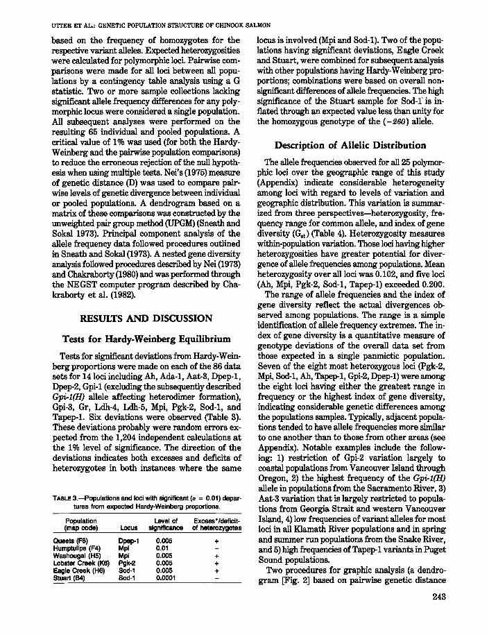
TABLE 3.-Populations and loci with significant (a = 0.01) depar­tures from expected Hardy-Weinberg proportions.

Tests for Hardy·Weinberg Equilibrium

Tests for significant deviations from Hardy-Wein­berg proportions were made on each of the 86 datasets for 14 loci including Ab, Ada-I, Aat-3, Dpep-l,Dpep-2, Gpi-l (excluding the subsequently describedGpi-1(H) allele affecting heterodimer formation),Gpi-3, Gr, Ldh-4, Ldh-5, Mpi, Pgk-2, Sod-I, andTapep-l. Six deviations were observed (Table 3).These deviations probably were random errors ex­pected from the 1,204 independent calculations atthe 1% level of significance. The direction of thedeviations indicates both excesses and deficits ofheterozygotes in both instances where the same

based on the frequency of homozygotes for therespective variant alleles. Expected heterozygositieswere calculated for polymorphic loci. Pairwise com­parisons were made for all loci between all popu­lations by a contingency table analysis using a Gstatistic. Two or more sample collections lackingsignificant allele frequency differences for any poly­morphic locus were considered a single population.All subsequent analyses were performed on theresulting 65 individual and pooled populations. Acritical value of 1% was used (for both the Hardy­Weinberg and the pairwise population comparisons)to reduce the erroneous rejection of the null hypoth­esis when using multiple tests. Nei's (1975) measureof genetic distance (D) was used to compare pair­wise levels of genetic divergence between individualor pooled populations. A dendrogram based on amatrix of these comparisons was constructed by the1lllweighted pair group method (UPGM) (Sneath andSokal 1973). Principal component analysis of theallele frequency data followed procedures outlinedin Sneath and Sokal (1973). A nested gene diversityanalysis followed procedures described by Nei (1973)and Chakraborty (1980) and was performed throughthe NEGST computer program described by Cha­kraborty et aI. (1982).

Description of Allelic Distribution

The allele frequencies observed for all 25 polymor­phic loci over the geographic range of this study(Appendix) indicate considerable heterogeneityamong loci with regard to levels of variation andgeographic distribution. This variation is summar­ized from three perspectives-heterozygosity, fre­quency range for common allele, and index of genediversity (Gst ) (Table 4). Heterozygosity measureswithin-population variation. Those loci having higherheterozygosities have greater potential for diver­gence of allele frequencies among populations. Meanheterozygosity over all loci was 0.102, and five loci(Ab, Mpi, Pgk-2, Sod-I, Tapep-l) exceeded 0.200.

The range of allele frequencies and the index ofgene diversity reflect the actual divergences ob­served among populations. The range is a simpleidentification of allele frequency extremes. The in­dex of gene diversity is a quantitative measure ofgenotype deviations of the overall data set fromthose expected in a single panmictic population.Seven of the eight most heterozygous loci (Pgk-2,Mpi, Sod-I, Ab, Tapep-l, Gpi-2, Dpep-l) were amongthe eight loci having either the greatest range infrequency or the highest index of gene diversity,indicating considerable genetic differences amongthe populations samples. Typically, adjacent popula­tions tended to have allele frequencies more similarto one another than to those from other areas (seeAppendix). Notable examples include the follow­ing: 1) restriction of Gpi-2 variation largely tocoastal populations from Vancouver Island throughOregon, 2) the highest frequency of the Gpi-l(H)allele in populations from the Sacramento River, 3)Aat-3 variation that is largely restricted to popula­tions from Georgia Strait and western VancouverIsland, 4) low frequencies of variant alleles for mostloci in all Klamath River populations and in springand summer r1lll populations from the Snake River,and 5) high frequencies of Tapep-l variants in PugetSound populations.

Two procedures for graphic analysis (a dendro­gram [Fig. 2] based on pairwise genetic distance

locus is involved (Mpi and Sod-I). Two of the popu­lations having significant deviations, Eagle Creekand Stuart, were combined for subsequent analysiswith other populations having Hardy-Weinberg pro­portions; combinations were based on overall non­significant differences of allele frequencies. The highsignificance of the Stuart sample for Sod-I'is in­flated through an expected value less than unity forthe homozygous genotype of the (- 260) allele.

0.005 +0.010.005 +0.005 +0.005 +0.0001

Level of Excess·/deficit-significance of heterozygotesLocus

Dpep-1MpiMpiPgk-2Sod-1Sod-1

Population(map code)

Queets (F6)HumptUlips (F4)Washougal (H5)Lobster Creek (K6)Eagle Creek (H6)Stuart (84)

243

FISHERY BULLETIN: VOL. 87, NO.2. 1989

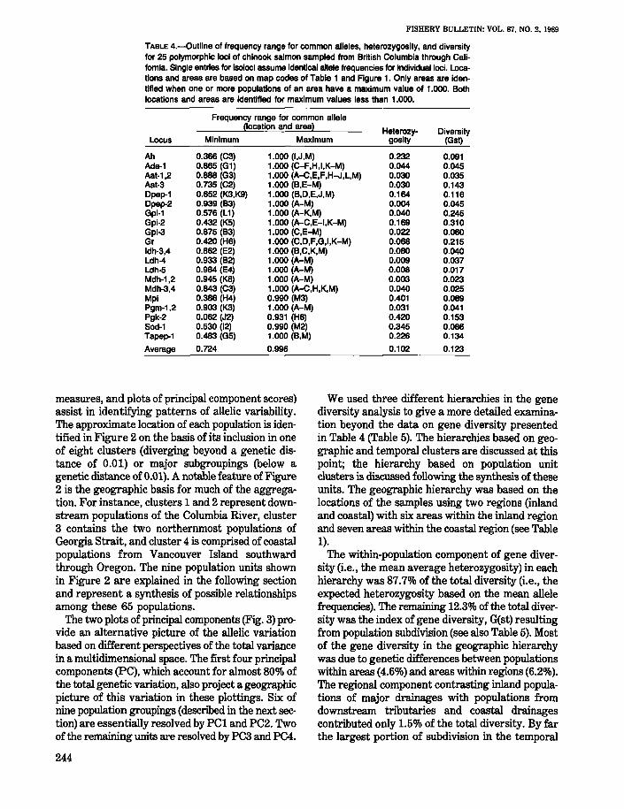
TABLE 4.-0utline of frequency range for common alleles, heterozygosity, and diversityfor 25 polymorphic loci of chinook salmon sampled from British Columbia through Cali-fomia. Single entries for isoloci assume identical allele frequencies for individual loci. Loca-tions and areas are based on map codes of Table 1 and Figure 1. Only areas are iden-tified when one or more populations of an area have a maximum value of 1.000. Bothlocations and areas are identified for maximum values less than 1.000.

Frequency range for common allele(location and area) Heterozy- Diversity

Locus Minimum Maximum gosity (Gst)

Ah 0.366 (C3) 1.000 (I,J.M) 0.232 0.091Ada-1 0.865 (G1) 1.000 (C-F,H,I,K-M) 0.044 0.045Aat-1,2 0.888 (G3) 1.000 (A-C,E,F,H-J,L,M) 0.030 0.035Aat-3 0.735 (C2) 1.000 (B,E-M) 0.030 0.143Dpep-1 0.652 (K3,K9) 1.000 (B,D,E,J,M) 0.164 0.116Dpep-2 0.939 (83) 1.000 (A-M) 0.004 0.045Gpi-1 0.576 (L1) 1.000 (A-K,M) 0.040 0.245Gpi-2 0.432 (K5) 1.000 (A-C,E-I,K-M) 0.169 0.310Gpi-3 0.875 (B3) 1.000 (C,E-M) 0.022 0.060Gr 0.420 (H6) 1.000 (C,D,F,G,I,K-M) 0.068 0.215Idh-3,4 0.862 (E2) 1.000 (B,C,K,M) 0.080 0.040Ldh-4 0.933 (B2) 1.000 (A-M) 0.009 0.037Ldh-5 0.964 (E4) 1.000 (A-M) 0.008 0.017Mdh-1,2 0.945 (K8) 1.000 (A-M) 0.003 0.023Mdh-3,4 0.843 (C3) 1.000 (A-e,H,K,M) 0.040 0.025Mpi 0.386 (H4) 0.990 (M3) 0.401 0.089pgm-1.2 0.903 (K3) 1.000 (A-M) 0.031 0.041Pgk-2 0.062 (J2) 0.931 (H6) 0.420 0.153Sod-1 0.530 (12) 0.990 (M2) 0.345 0.086Tapep-1 0.483 (G5) 1.000 (B,M) 0.226 0.134

Average 0.724 0.996 0.102 0.123

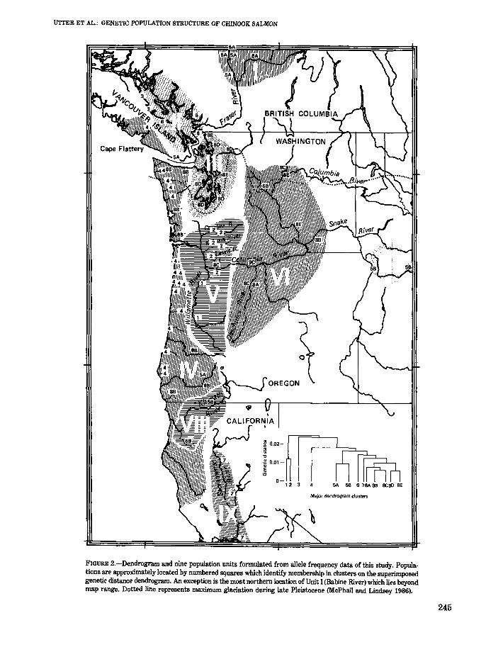
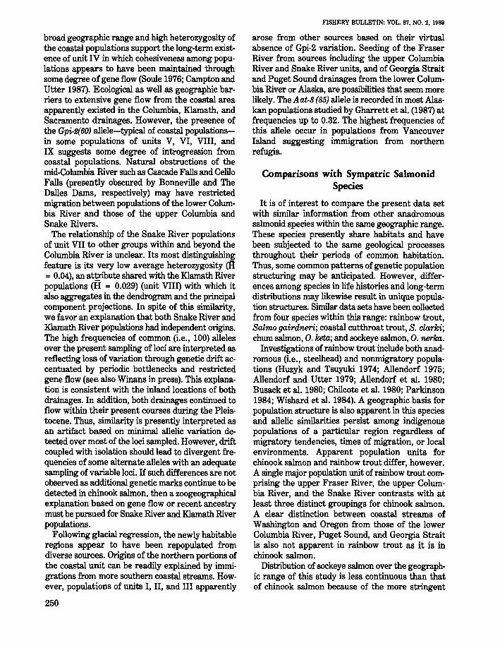
measures, and plots of principal component scores)assist in identifying patterns of allelic variability.The approximate location of each population is iden­tified in Figure 2 on the basis of its inclusion in oneof eight clusters (diverging beyond a genetic dis­tance of 0.01) or major subgroupings (below agenetic distance of 0.01). A notable feature of Figure2 is the geographic basis for much of the aggrega­tion. For instance, clusters 1 and 2 represent down­stream populations of the Columbia River, cluster3 contains the two northernmost populations ofGeorgia Strait, and cluster 4 is comprised of coastalpopulations from Vancouver Island southwardthrough Oregon. The nine population units shownin Figure 2 are explained in the following sectionand represent a synthesis of possible relationshipsamong these 65 populations.

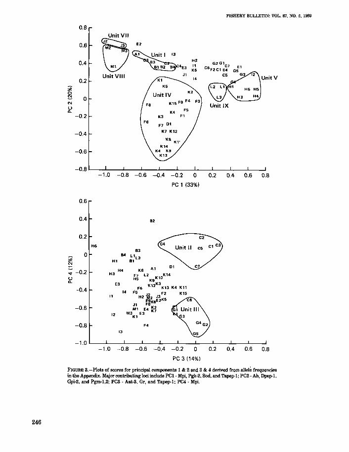
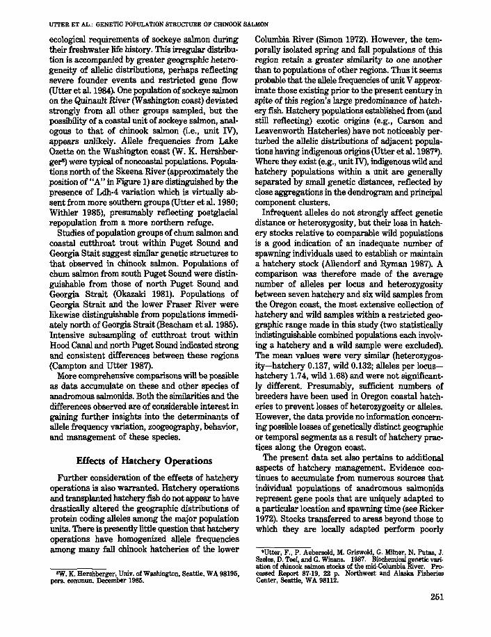
The two plots of principal components (Fig. 3) pro­vide an alternative picture of the allelic variationbased on different perspectives of the total variancein a multidimensional space. The first four principalcomponents (PC), which account for almost 80% ofthe total genetic variation, also project a geographicpicture of this variation in these plottings. Six ofnine population groupings (described in the next sec­tion) are essentially resolved by PC1 and PC2. Twoof the remaining units are resolved by PC3 and PC4.

244

We used three different hierarchies in the genediversity analysis to give a more detailed examina­tion beyond the data on gene diversity presentedin Table 4 (Table 5). The hierarchies based on geo­graphic and temporal clusters are discussed at thispoint; the hierarchy based on population unitclusters is discussed following the synthesis of theseunits. The geographic hierarchy was based on thelocations of the samples using two regions (inlandand coastal) with six areas within the inland regionand seven areas within the coastal region (see Table1).

The within-population component of gene diver­sity (i.e., the mean average heterozygosity) in eachhierarchy was 87.7% of the total diversity (i.e., theexpected heterozygosity based on the mean allelefrequencies). The remaining 12.3% of the total diver­sity was the index of gene diversity, G(st) resultingfrom population subdivision (see also Table 5). Mostof the gene diversity in the geographic hierarchywas due to genetic differences between populationswithin areas (4.6%) and areas within regions (6.2%).The regional component contrasting inland popula­tions of major drainages with populations fromdownstream tributaries and coastal drainagescontributed only 1.5% of the total diversity. By farthe largest portion of subdivision in the temporal

UTTER ET AL.: GENETIC POPULATION STRUCTURE OF CHINOOK SALMON

g 0.02­

~'0.~ 0.01­

~

"SA 5S 6 78A SS IlCBO SE

Maj()r r.rendro(jtam clustel'5

FIGURE 2.-Dendrogram and nine population units fonnulated from allele frequency data of this study. Popula­tions are approximately located by numbered squares which identify membership in clusters on the superimposedgenetic distance dendrogram. An exception is the most northern location of Unit I (Babine River) which lies beyondmap range. Dotted line represents maximum glaciation during late Pleistocene (McPhail and Lindsey 1986).

245

FISHERY BULLETIN: VOL. 87, NO.2. 1989

0.8Unit VII

00.6 M2 J3E2

0.4 H2G2 G1

C7M1 4E3 11K6 C6 F2 Cl E4

Unit VIII Jl C5UnitV0.2 14

?i. 0 1 H6 H50 Unit IV~ 0 L3 H4

N K15 F9 F4Unit IXu

ll.. K4F5

-0.2 K3 Fl

F7 01

-0.4 K7 K12

-0.6

-0.8-1.0 -0.8 -0.6 -0.4 -0.2 0 0.2 0.4 0.6 0.8

PC 1 (33%)

0.6

0.4 82

0.2

H683

0 84 L1 L3

*" HI 81N::::. Al 01

-0.2 H4 K6.... H3 F7 L2 K14U H5 K9

K1Oll.. E3

K12K3

K13 K4 Kll-0.4 F6

14 1'5 J2 F2 K1511 H2 M2 J3

F9KSE2K5

-0.6J1 FSMl E4 K2

12 M3 E3 K7Kl

-0.8 F4

13

-1.0-1.0 -0.8 -0.6 -0.4 -0.2 0 0.2 0.4 0.6 0.8

PC 3 (14%)

FIGURE 3.-Plots of scores for principal components 1 & 2 and 3 & 4 derived from allele frequenciesin the Appendix. Major contributing loci include PCI - Mpi, Pgk-2, Sod. and Tapep-l; PC2 - Ah, Dpep·l.Gpi-2. and Pgm-l.2; PC3 - Aat-3. Gr, and Tapep-l; PC4 - Mpi.

246

UTTER ET AL.: GENETIC POPULATION STRUCTURE OF CHINOOK SALMON

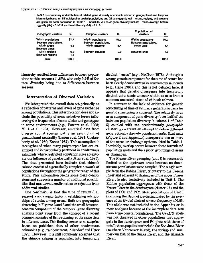
TABLE 5.-Summary of distribution of relative gene diversity of chinook salmon in geographical and temporalhierarchies based on 65 individual or pooled populations and 25 polymorphic loci. Areas, regions, and seasonsare given for each population in Table 1. Absolute values of gene diversity include mean average hetero­zygosity (Hs) • 0.1018 and total diversity (Ht) - 0.1161.

Population unitGeographic clusters % Temporal clusters % Clusters %

Within populations 87.7 Within populations 87.7 Within populations 87.7Between populations, Between populations, Between populations,

within areas 4.6 within seasons 11.4 within units 4.4Between areas,

within regions 6.2 Between seasons 0.9 Between units 7.9Between regions 1.5

Total 100.0 100.0 100.0

hierarchy resulted from differences between popula­tions within seasons (11.6%), with only 0.7% of thetotal diversity being due to differences betweenseasons.

Interpretation of Observed Variation

We interpreted the overall data set primarily asa reflection of patterns and levels of gene exchangeamong populations. This interpretation does not ex­clude the possibility of some selective forces influ­encing the frequencies of some alleles and genotypesin some environments (e.g., Powers et al. 1983;Mork et al. 1984). However, empirical data fromdiverse animal species justify an assumption ofpredominant neutrality (Ihssen et al. 1981; Chakra­borty et al. 1980; Eanes 1987). This assumption isstrengthened when many polymorphic loci are ex­amined and is particularly pertinent in anadromoussalmonids where restricted population sizes accentu­ate the influence of genetic drift (Utter et al. 1980).The data presented here indicate that chinooksalmon consist of a genetically complex network ofpopulations throughout the geographic range of thisstudy. This information yields some clear conclu­sions and suggests a number of additional possibil­ities that must await confirmation or rejection fromadditional studies.

One conclusion is that the time of return (i.e.,season) is not a major factor in establishing relation­ships of stocks among areas. Both the geographicclustering in Figures 2 and 3 and the small between­seasons component of the temporal gene diversityanalysis point away from the concept of a recentcommon ancestry of fish returning at the same timein different areas. This finding comes as no surprisebased on published data of other anadromoussalmonids (e.g., rainbow trout, Allendorf and Utter1979). However, it is still commonly accepted thatthe chinook salmon is separated into temporally

distinct "races" (e.g., McClane 1978). Although astrong genetic component for the time of return hasbeen clearly demonstrated in anadromous salmonids(e.g., Helle 1981), and this is not debated here, itappears that genetic divergence into temporallydistinct units tends to occur within an area from acommon ancestral stock of chinook salmon.

In contrast to the lack of evidence for geneticstructuring of time of return, a geographic basis forgenetic structuring is apparent. The relatively largearea component of gene diversity (over half of thebetween-population diversity in column 1 of Table5) coupled with the predominantly geographicclusterings warrant an attempt to define differentgeographically discrete population units. Most units(Figure 2 and Appendix) incorporate one or moreof the areas or drainage systems listed in Table 1.Inevitably, overlap occurs between these formulatedpopulation units and the a priori groupings of areasor drainages.

The Fraser River grouping (unit I) is necessarilylimited to the upstream areas because no down­stream populations were sampled. The single sam­ple from the Babine River, tributary to the SkeenaRiver and adjacent to drainages of the upper FraserRiver, is also tentatively included in Unit I. TheBabine population aggregates with those of theFraser River in the dendrogram (cluster 5A) and theplots of PC1 and PC2. Most populations of Unit I(including the Babine) are distinguished by the pres­ence of the Gr-ll0 allele at a mean frequency of 0.05.This allele was not included in the Appendix or inmost analyses because of the incomplete data setsfrom some coastal populations. The Gr-(1lO) allelewas not observed in other populations that aggre­gate in the dendrogram and PC plots with those ofunit I; these populations include the San Juan River(southern Vancouver Island), the spring- and sum­mer-run fish of the Snake River, and the KlamathRiver.

247

The population unit of Georgia Strait (unit II) com­prises populations forming clusters 3 and 6 in thedendrogram, plus the San Juan River population.These six populations aggregate adjacently in theplottings of PC3 and PC4. Populations of Unit IItypically have relatively high allele frequencies ofAat-3 (90), Pkg-2 (90), and Tapep-l (130), althoughexceptions occur at each locus. Carl and Healey(1984) reported similar high frequencies for allelicvariations of Aat-3 and Tapep in a study of chinooksalmon populations of the Nanaimo River whichflows from Vancouver Island into Georgia Strait.

Populations in the Puget Sound unit (Unit III),bounded to the north by the population from theSouth Fork of the Nooksack River, aggregate fair­ly clearly in both the dendrogram (clusters 8D and8E) and the plots of PC3 and PC4. The cohesivenessamong the fall-run populations vary likely reflectsboth genetic isolation and present (or very recent)gene flow through transfers among hatcheries. Likeunit II, populations of unit III also have high allelefrequencies for Tapep-1130; in fact, it has the high­est mean frequencies for this allele among the ninepopulation units that were formulated. However, themean frequencies of the common (i.e., 100) allelesfor Aat-3 and Pgk-2 are much higher in unit III thanin unit II. No influence of reported transfers of lowerColumbia River fish to Puget Sound hatcheries (e.g.,Ricker 1972) is apparent from the graphic projec­tions or the allelic data.

An extended grouping of coastal populations (unitIV) ranges from northern California (see Utter etal. 1980) to Robertson Creek on the west coast ofVancouver Island. Populations of the Columbia,Klamath, and Sacramento Rivers are excluded fromunit IV. This unit is distinguished by high frequen­cies of the Gpi-2 (60) allele and (in most instances)some Pgm variation. Most populations appear eitherin clusters 4 or 8B of the dendrogram and aggregatedistinctly in the plottings of PCl and PC2. Twopopulations are retained in Unit IV for geographicconsistency which do not congregate with otherpopulations of this unit; the spring run returning tothe Soleduck River on the Washington coast, andthe Lobster Creek population returning to the upperRogue River on the Oregon coast. The outlying ofthe Soleduck spring-run population appears to berelated to its heterogeneous origins. Records in­dicate that this run originated from crosses of fishfrom the Cowlitz River Qower Columbia River) andUmpqua River (Oregon coast) with some contribu­tion from the spring run of the Dungeness River,a drainage entering the Strait of Juan de Fuca (C.Johnson6). An explanation for the outlying of the

248

FISHERY BULLETIN: VOL. 87, NO.2, 1989

Lobster Creek population is less apparent and re­quires further investigation.

Two individual and four paired hatchery popula­tions sampled from the lower Columbia River forma geographically and genetically discrete unit (unitV). This group represents the most divergent pairof clusters (1 and 2) on the dendrogram and general­ly aggregates distinctly in the plotting of PCl andPC2. Populations of unit V are particularly distin­guished by high allele frequencies of Gr (85) and Mpi(109). Unit V is bounded upstream by the U.S. Fishand Wildlife Service Spring Creek Hatchery popu­lation (Spring Creek Hatchery is located on the poolimpounded by Bonneville Dam). The pairing of fourof the six populations is consistent with high levelsof gene flow resulting from an extensive history oftransplantation among the populations of the lowerColumbia River (Simon 1972; Howell et al. 1985).This group's distinctness from other groups is alsoconsistent with a minimal impact of transplantationsof these populations beyond the lower ColumbiaRiver on indigenous populations in other areas (e.g.,Cowlitz spring-run fish to the Snake River. C.Burley6; Kalama fall-run fish to Puget Sound, men­tioned above).

The upper Columbia River unit (unit VI)-morethan any of the other groupings-is composed ofgenetically diverse elements placed together moreon the basis of geographic convenience rather thangenetic unity. Unit VI is somewhat loosely boundeddownstream by populations of the Klickitat andDeschutes Rivers; both rivers enter the ColumbiaRiver near The Dalles Dam. Unit VI's componentpopulations include individuals of mixed ancestralorigins, along with others of presumably pure line­age. Two populations known to have mixed ances­tral origin are those of the U.S. Fish and WildlifeService Carson and Leavenworth Hatcheries. TheCarson Hatchery population Qocated on the WindRiver which drains into the Bonneville pool) wasderived from interceptions of spring-run fishdestined for areas of the upper Columbia and SnakeRivers. The Leavenworth population (combined withCarson in the analyses) has been largely maintainedby continued infusions from fish of the CarsonHatchery (Howell et al. fn. 5). The Ice Harbor pop­ulation-another group of mixed ancestral origins­is composed of fall-run fish destined for differentareas within the Snake River that were interceptedat Ice Harbor Dam near the mouth of the Snake

·C. Johnson, Washington Department of Fisheries. General Ad­ministration Bldg.. Olympia. WA 98504, pers. commun. May 1985.

·C. Burley, U.S. Fish and Wildlife Service, 9317 Highway 99,Vancouver. WA 98665. pers. commun. May 1985.

U'ITER ET AL.: GENETIC POPULATION STRUCTURE OF CHINOOK SALMON

River. This population is included in unit VI becauseof its geographic proximity and genetic similarityto populations of unit VI contrasted with its dis­tinctness from spring- and summer-run populationsof the upper Snake River.

Populations of purer lineage within unit VI aggre­gate within cluster 8 of the dendrogram. The spring­run population returning to the Lewis River liesgeographically within unit V. entering the Colum­bia River below Bonneville Dam. This population isincluded in unit VI because it is genetically distinctfrom other downstream populations and moretypical of certain spring- and fall-run fish within UnitVI (Le., Klickitat, Deschutes, and Winthrop popu­lations) with which it closely aggregates on the den­drogram (cluster 8C) and the plots of PC1 and PC2.

The similarity of the populations from Wells Damand Priest Rapids Dam in unit VI is presumably areflection of the two groups being different temporalsegments of the same major run. All fish migratingpast Priest Rapids Dam prior to 13 August are per­mitted to pass upstream and sequentially constitutethe spring- and summer-runs of the upper Colum­bia River. The latter segment of this migration ar­riving at Wells Dam is captured and spawned forhatchery production. Most arrivals at Priest RapidsDam later than 14 August are intercepted andspawned there (Chris Carlson7). This process inevi­tably results in considerable gene flow betweenthese two artificially maintained populations.

The Snake River unit (unit VII) contains the twocombined populations of McCall Hatchery-JohnsonCreek and Rapid River Hatchery-Valley Creek­Sawtooth-Red River, all managed by the IdahoDepartment of Fish and Game; all populations arefrom the Salmon River drainage of central Idaho.This unit is distinguished by very low averageheterozygosities (see Winans in press) and by highfrequencies of the Pgk-2 (90) allele.

The Klamath River populations (unit VIII) aregeographically isolated from, but genetically similarto those of the Snake River. However, populationsof unit VIII lack variation of Idh-3,4 contrasted witha mean frequency of 0.925 for the Idh-8,J, (100) allelein unit VII. Klamath River populations, like thoseof unit VII, are characterized by very low aver­age heterozygosities. This characteristic contrastssharply with most adjacent coastal populations forwhich the highest heterozygosities among all popu­lations are observed. Allele frequency data from theShasta and Scott river populations, two wild pop-

7Chris Carlson. Grant County Public Utility District. P.O. Box878. Ephrata. WA 98823. p~rs. commun. March 1986.

ulations of the Klamath River are statistically iden­tical with frequencies in the Iron Gate Hatcherysample; these data were recently collected whichprecluded their use in most of the analyses of thisstudy. Thus the low heterozygosity of Klamath Riverpopulations cannot be attributed to effects of.hatch­ery management (see Allendorf and Ryman 1987).

The three samples from the Sacramento ·Riverdrainage form a distinct geographic and genetic unit(unit IX). These samples cluster together in the den­drogram (cluster 7) and in PC1 and PC2. As men­tioned above, these populations are distinguished byhigh frequencies of the Gpi-l(H) allele.

An analysis of gene diversity within and betweenthe nine proposed population units (Table 5, column3), provides further support for the reality of thesegenetic subdivisions. It is appropriate that almosttwo-thirds of the total gene diversity due to popula­tion structuring (7.9/12.3 = 64.2%) occurred be­tween the population units. Furthermore, thediversity between populations within the units wassmaller than the diversity between populationswithin areas (Table 5. column 1) calculated prior tothe synthesis of the units.

Relationships and Origins ofPopulation Units

The common genetic and geographic attributes ofpopulations within units have been stressed, butrelationships between units also require considera­tion. The geographic areas of the Fraser River,Georgia Strait, and Puget Sound (units I, II, and III)were completely glaciated during the late Pleisto­cene, and therefore must have been entirely re­populated within roughly the last 15,000 years(McPhail and Lindsey 1986). Those areas of theColumbia River sampled in this study were outsideof the ice sheet, although the upper third of thedrainage was glaciated. However, downstream pop­ulations (units V and VI) were doubtlessly affectedby massive runoffs and temporary impoundmentsresulting from sudden releases of glacial Lake Mis­soula initially occurring some 18,000 years ago(Bunker 1982); most of the Snake River drainage(unit VII), entering the mid-Columbia River fromthe south, was presumably unaffected by theseevents above its lower reaches. The coastal region(Unit IV) from the Chehalis River (Washington)southward, and the entire Sacramento-San JoaquinRiver drainage (unit III), were likewise free ofglaciation during the late Pleistocene.

Much of the presently observed genetic diversityalmost certainly existed during the Pleistocene. The

249

broad geographic range and high heterozygosity ofthe coastal populations support the long-term exist­ence of unit IV in which cohesiveness among popu­lations appears to have been maintained throughsome degree of gene flow (Soule 1976; Campton andUtter 1987). Ecological as well as geographic bar­riers to extensive gene flow from the coastal areaapparently existed in the Columbia, Klamath, andSacramento drainages. However, the presence ofthe Gpi-2(60J allele-typical of coastal populations­in some populations of units V, VI, VIII, andIX suggests some degree of introgression fromcoastal populations. Natural obstructions of themid-Columbia River such as Cascade Falls and CeliloFalls (presently obscured by Bonneville and TheDalles Dams, respectively) may have restrictedmigration between populations of the lower Colum­bia River and those of the upper Columbia andSnake Rivers.

The relationship of the Snake River populationsof unit VII to other groups within and beyond theColumbia River is unclear. Its most distinguishingfeature is its very low average heterozygosity (R= 0.04), an atgibute shared with the Klamath Riverpopulations (H = 0.029) (unit VIII) with which italso aggregates in the dendrogram and the principalcomponent projections. In spite of this similarity,we favor an explanation that both Snake River andKlamath River populations had independent origins.The high frequencies of common (i.e., 100) allelesover the present sampling of loci are interpreted asreflecting loss of variation through genetic drift ac­centuated by periodic bottlenecks and restrictedgene flow (see also Winans in press). This explana­tion is consistent with the inland locations of bothdrainages. In addition, both drainages continued toflow within their present courses during the Pleis­tocene. Thus, similarity is presently interpreted asan artifact based on minimal allelic variation de­tected over most of the loci sampled. However, driftcoupled with isolation should lead to divergent fre­quencies of some alternate alleles with an adequatesampling of variable loci. If such differences are notobserved as additional genetic marks continue to bedetected in chinook salmon, then a zoogeographicalexplanation based on gene flow or recent ancestrymust be pursued for Snake River and Klamath Riverpopulations.

Following glacial regression, the newly habitableregions appear to have been repopulated fromdiverse sources. Origins of the northern portions ofthe coastal unit can be readily explained by immi­grations from more southern coastal streams. How­ever, populations of units I, II, and III apparently

250

FISHERY BULLETIN: VOL. 87, NO.2, 1989

arose from other sources based on their virtualabsence of Gpi-2 variation. Seeding of the FraserRiver from sources including the upper ColumbiaRiver and Snake River units, and of Georgia Straitand Puget Sound drainages from the lower Colum­bia River or Alaska, are possibilities that seem morelikely. The Aa.t-9 (85) allele is recorded in most Alas­kan populations studied by Gharrett et al. (1987) atfrequencies up to 0.32. The highest frequencies ofthis allele occur in populations from VancouverIsland suggesting immigration from northernrefugia.

Comparisons with Sympatric SalmonidSpecies

It is of interest to compare the present data setwith similar information from other anadromoussalmonid species within the same geographic range.These species presently share habitats and havebeen subjected to the same geological processesthroughout their periods of common habitation.Thus, some common patterns of genetic populationstructuring may be anticipated. However, differ­ences among species in life histories and long-termdistributions may likewise result in unique popula­tion structures. Similar data sets have been collectedfrom four species within this range: rainbow trout,Salmo gairdneri; coastal cutthroat trout, S. clarki;chum salmon, O. keta; and sockeye salmon, O. nerka.

Investigations of rainbow trout include both anad­romous (i.e., steelhead) and nonmigratory popula­tions (Huzyk and Tsuyuki 1974; Allendorf 1975;Allendorf and Utter 1979; Allendorf et al. 1980;Busack et al. 1980; Chilcote et al. 1980; Parkinson1984; Wishard et al. 1984). A geographic basis forpopulation structure is also apparent in this speciesand allelic similarities persist among indigenouspopulations of a particular region regardless ofmigratory tendencies, times of migration, or localenvironments. Apparent population units forchinook salmon and rainbow trout differ, however.A single major population unit of rainbow trout com­prising the upper Fraser River, the upper Colum­bia River, and the Snake River contrasts with atleast three distinct groupings for chinook salmon.A clear distinction between coastal streams ofWashington and Oregon from those of the lowerColumbia River, Puget Sound, and Georgia Straitis also not apparent in rainbow trout as it is inchinook salmon.

Distribution of sockeye salmon over the geograph­ic range of this study is less continuous than thatof chinook salmon because of the more stringent

UTTER ET AL.: GENETIC POPULATION STRUCTURE OF CHINOOK SALMON

ecological requirements of sockeye salmon duringtheir freshwater life history. This irregular distribu­tion is accompanied by greater geographic hetero­geneity of allelic distributions, perhaps reflectingsevere founder events and restricted gene flow(Utter et al. 1984). One population of sockeye salmonon the Quinault River (Washington coast) deviatedstrongly from all other groups sampled, but thepossibility of a coastal unit of sockeye salmon, anal­ogous to that of chinook salmon (Le., unit IV),appears unlikely. Allele frequencies from LakeOzette on the Washington coast (W. K. Hershber­gerS) were typical of noncoastal populations. Popula­tions north of the Skeena River (approximately theposition of HAlO in Figure 1) are distinguished by thepresence of Ldh-4 variation which is virtually ab­sent from more southern groups (Utter et al. 1980;Withler 1985), presumably reflecting postglacialrepopulation from a more northern refuge.

Studies of population groups of chum salmon andcoastal cutthroat trout within Puget Sound andGeorgia Stait suggest similar genetic structures tothat observed in chinook salmon. Populations ofchum salmon from south Puget Sound were distin­guishable from those of north Puget Sound andGeorgia Strait (Okazaki 1981). Populations ofGeorgia Strait and the lower Fraser River werelikewise distinguishable from populations immedi­ately north of Georgia Strait (Beacham et al. 1985).Intensive subsampling of cutthroat trout withinHood Canal and north Puget Sound indicated strongand consistent differences between these regions(Campton and Utter 1987).

More comprehensive comparisons will be possibleas data accumulate on these and other species ofanadromous salmonids. Both the similarities and thedifferences observed are of considerable interest ingaining further insights into the determinants ofallele frequency variation, zoogeography, behavior,and management of these species.

Effects of Hatchery Operations

Further consideration of the effects of hatcheryoperations is also warranted. Hatchery operationsand transplanted hatchery fish do not appear to havedrastically altered the geographic distributions ofprotein coding alleles among the major populationunits. There is presently little question that hatcheryoperations have homogenized allele frequenciesamong many fall chinook hatcheries of the lower

trW. K. Hershberger, Univ. of Washington, Seattle, WA 98195,pers. commun. December 1985.

Columbia River (Simon 1972). However, the tem­porally isolated spring and fall populations of thisregion retain a greater similarity to one anotherthan to populations of other regions. Thus it seemsprobable that the allele frequencies of unit V approx­imate those existing prior to the present century inspite of this region's large predominance of hatch­ery fish. Hatchery populations established from (andstill reflecting) exotic origins (e.g., Carson andLeavenworth Hatcheries) have not noticeably per­turbed the allelic distributions of adjacent popula­tions having indigenous origins (Utter et a1. 19871l).

Where they exist (e.g., unit IV), indigenous wild andhatchery populations within a unit are generallyseparated by small genetic distances, reflected byclose aggregations in the dendrogram and principalcomponent clusters.

Infrequent alleles do not strongly affect geneticdistance or heterozygosity, but their loss in hatch­ery stocks relative to comparable wild populationsis a good indication of an inadequate number ofspawning individuals used to establish or maintaina hatchery stock (Allendorf and Ryman 1987). Acomparison was therefore made of the averagenumber of alleles per locus and heterozygositybetween seven hatchery and six wild samples fromthe Oregon coast, the most extensive collection ofhatchery and wild samples within a restricted geo­graphic range made in this study (two statisticallyindistinguishable combined populations each involv­ing a hatchery and a wild sample were excluded).The mean values were very similar (heterozygos­ity-hatchery 0.137, wild 0.132; alleles per locus­hatchery 1.74, wild 1.68) and were not significant­ly different. Presumably, sufficient numbers ofbreeders have been used in Oregon coastal hatch­eries to prevent losses of heterozygosity or alleles.However, the data provide no information concern­ing possible losses of genetically distinct geographicor temporal segments as a result of hatchery prac­tices along the Oregon coast.

The present data set also pertains to additionalaspects of hatchery management. Evidence con­tinues to accumulate from numerous sources thatindividual populations of anadromous salmonidsrepresent gene pools that are uniquely adapted toa particular location and spawning time (see Ricker1972). Stocks transferred to areas beyond those towhich they are locally adapted perform poorly

'Utter, F., P. Aebersold, M. Griswold, G. Milner, N. Putas, J.Szeles, D. Teel, and G. Winans. 1987. Biochemical genetic vari­ation of chinook salmon stocks of the mid-Columbia River. Pro­cessed Report 87-19. 22 p. Northwest and Alaska FisheriesCenter, Seattle, WA 98112.

251

relative to indigenous populations (Withler 1982;Altukhov and Salmenkova 1987; Reisenbichler1988). Transfers from maladapted populations notonly waste effort and resource, but also carry therisk of disrupting locally adapted genomes throughinterbreedings (Reisenbichler and McIntyre 1977;Shields 1982). Sets of data such as those reportedhere are valuable in outlining at least the maximumdistribution of locally adapted gene pools and there­by provide guidelines for stock transfers. In theabsence of any other data, it would be inadvisableto translocate populations between sites such as thelower Columbia River and the Washington or Ore­gon coasts.

Stock transfers within major genetic units shouldalso be performed with caution. Each of the indivi­dual or pooled populations within the nine units isalso genetically distinct for some loci sampled in thisstudy from other populations within the unit; theyare therefore divergent from such populations at amuch larger number of additional loci throughoutthe genome. It is pertinent to recall that a consid­erable amount of the total gene diversity resultsfrom population subdivision (4.4112.3 = 35.8%)resided within the population units (Table 5, column3). Likewise, slight or no divergence between twopopulations based on samplings of polymorphic pro­tein-coding loci does not necessarily mean thesepopulations are identically adapted (discussed inUtter 1981). For example, two groups of rainbowtrout in the Snake River drainage having similarallele frequencies at five polymorphic loci areadapted to drastically different local environmentsand life history patterns (Wishard et al. 1984).

CONCLUDING OBSERVATIONS

Three points require emphasis following this ini­tial outline of population units. First, it warrantsrestating that each of the nine units represents agenetically heterogeneous grouping. It is importantthat this heterogeneity be recognized and main­tained within the respective units.

Second, these units are based on limited datawithin the range of sampling and, in some instances,on arbitrary decisions; the units are intended to bemodified as more information accumulates andtherefore to serve as guidelines for further inves­tigation. For purposes of clarification, allelic databeyond those listed in the Appendix have been intro­duced at various places in the text. Additional allelesand polymorphic protein-coding loci are continual­ly being identified through ongoing investigations,and further clarification is inevitable as these data

252

FISHERY BULLETIN: VOL. 87. NO.2. 1989

accumulate. Genetic data other than from protein­coding loci are accumulating on chinook salmonpopulations within the geographic range of thisstudy. Such genetic data show differences amongpopulations in mitochondrial DNA (E. Berming­hamID), and life history variables (Nicholas andHankin 1988; Schreck et al. 1986), and provide com­plementary insights that will ultimately result in amuch more detailed understanding of genetic struc­turing of these chinook salmon populations.

Third, numerous distinct population units exist inNorth America beyond the sampling area of thisstudy (e.g., Gharrett et al. 1987) and nothing isknown of Asiatic populations. The nine units pre­sented here, then, are viewed as a necessary partof a much more complete picture of the geneticstructure of chinook salmon that will ultimatelyemerge.

ACKNOWLEDGMENTS

Assistance in sampling was provided by person­nel of agencies including the Canadian Departmentof Fisheries and Oceans, California Department ofFish and Game, Oregon Department of Fisheriesand Wildlife, and Washington Department of Fish­eries. Valuable technical assistance was provided byP. Aebersold. Valuable reviews were provided byC. Mahnken, G. Winans, A. Gharrett, Northwestand Alaska Fisheries Center and three anonymousreviewers.

LITERATURE CITED

AEBERSOLD. P. B.. G. A. WINANS. D. J. TEEL, G. B. MILNER,AND F. M. UTTER.

1987. Manual for starch gel electrophoresis: A method forthe detection of genetic variation. U.S. Dep. Commer.,NOAA Tech. Rep. NMFS 61, 19 p.

ALLENDORF. F. W.1975. Genetic variability in a species possessing extensive

gene duplication: Genetic interpretation of duplicate loci andexamination of genetic variation in populations of rainbowtrout. Ph.D. Thesis. Univ. Washington, Seattle. 98 p.

ALLENDORF, F. W., D. M. ESPELAND, D. T. Scow. AND S. PHELPS.1980. Coexistence of native and introduced rainbow trout in

the Kootenai River drainage. Proc. Mont. Acad. Sci. 39:28-36.

ALLENDORF. F. W., AND N. RYMAN.1987. Genetic management ofhatchery stocks. 171 N. Ryman

and F. M. Utter (editors), Population genetics and fisherymanagement. p. 141-159. Univ. Wash. Press, Seattle.

ALLENDORF, F. W., AND G. H. THORGAARD.1984. Tetraploidy and the evolution of salmonid fishes. In

B. Turner (editor), Evolutionary genetics offishes. p. 1-53.

lOE. Bermingham. NMFS, 2725 Montlake Boulevard East,Seattle. WA 98112. pers. commun. November 1987.

UTIER ET AL.: GENETIC POPULATION STRUCTURE OF CHINOOK SALMON

Plenum Press, N.Y.ALLENDORF. F. W., AND F. M. UTTER.

1979. Population genetics. In W. S. Hoar, D. J. Randall, andR. Brett (editors), Fish physiology, Vol. 8. p. 407-454.Acad. Press, N.Y.

ALTUKHOV, Y. P .• AND E. A. SALMENKOVA.1987. Stock transfer relative to natural organization. man­

agement, and conservation of fish populations. In· N.Ryman and F. M. Utter (editors), Population genetics andfishery management. p. 33-343. Univ. Wash. Press,Seattle.

BEACHAM, T.• R. WITHLER, AND A. GOULD.1985. Biochemical genetic stock identification of chum salmon

(OrworhynchlUl ketal in southern British Columbia. Can. J.Fish. Aquat. Sci. 42:437-448.

BOYER, S. H., D. C. FAINER, AND E. J. WATSON-WILLIAMS.1963. Lactate dehydrogenase variant from human blood:

Evidence for molecular subunits. Science 141:642-643.BUNKER, R. C.

1982. Evidence of multiple late-Wisconsin floods from glacialLake Missoula in Badger Coulee. Washington. Q. Res. (NY)18:17-31.

BUSACK. C. A.• G. H. THORGAARD, M. P. BANNON. AND G. A. E.GALL.

1980. An electrophoretic, karyotypic and meristic character­ization of the Eagle Lake trout, Salmo gairdneM aqltilarunt.Copeia 1980:418-424.

CAMPTON. D. C., AND F. M. UTTER.1987. Genetic structure of anadromous cutthroat trout

(Salmo clarki clarki) populations in two Puget Soundregions: Evidence for restricted gene flow. Can. J. Fish.Aquat. Sci. 44:573-582.

CARL, L. M.. AND M. C. HEALEY.1984. Differences in enzyme frequency and body morphology

among three juvenile life history types of chinook salmon(Orw./)'/"kyttchtIS l$kawytsclla) in the Nanaimo River, BritishColumbia. Can. J. Fish. Aquat. Sci. 41:1070-1077.

CHAKRABORTY. R.1980. Gene diversity analysis in nested subdivided popula­

tions. Genetics 96:721-726.CHAKRABORTY, R.. P. A. FUERST, AND M. NEI.

1980. Statistical studies on protein polymorphism in naturalpopulations Ill. Distribution of allele frequencies and thenumber of alleles per locus. Genetics 94:1039-1063.

CHAKRABORTY. R., M. HAGG, N. RYMAN, AND G. STAHL.1982. Hierarchical gene diversity analysis and its application

to brown trout population data. Hereditas 97:17-21.CHILCOTE, M. Woo B. A. CRAWFORD. AND S. A. LEIDER.

1980. A genetic comparison of sympatric populations of sum­mer and winter steelheads. Trans. Am. Fish. Soc. 109:203-206.

CLAYTON. J. W., AND D. N. TRETIAK.1972. Amine-citrate buffers of pH control in starch gel elec­

trophoresis. J. Fish. Res. Board Can. 29:1169-1172.EANES, W. F.

1987. Allozymes and fitness: Evolution of a problem. TrendsEvol. Ecol. 2(2):44-48.

GHARRETT. A. J., S. M. SHIRLEY. AND G. R. TROMBLE.1987. Genetic relationships among populations of Alaskan

chinook salmon (Orworkynchus tBhau'ytBcha). Can. J. Fish.Aquat. Sci. 44:765-774.

HARRIS, H., AND D. A. HOPKINSON.1976. Handbook of enzyme electrophoresis in human gene­

tics. Am. Elsevier. N.Y.HELLE, J. H.

1981. Significance of the stock concept in artificial propa-

gation of salmonids in Alaska. Can. J. Fish. Aquat. Sci.38:1665-1671.

HOWELL. P .• K. JONES. D. SCARNECCHIA. L. LAVAY. W. KENDRA,AND D. ORTMANN.

1985. Stock assessment of Columbia River anadromoussalmonids. I. chinook, coho, chum and sockeye salmon stocksummaries. Final report to Bonneville Power Administra­tion on contract No. DE-A1179-84BPI2737. 558 p. Avail­able from Bonneville Power Administration. P.O. Box 3621,Portland. OR 97208.

HUZYK, L., AND H. TSUYUKI.1974. Distribution of Ldh-B gene in resident and anadromous

rsinbow trout (Salnw gairdlleM) from streams in British Col­umbia. J. Fish. Res. Board Can. 31:106-108.

IHSSEN. P. E., H. E. BOOKE, J. M. CASSELMAN. J. M. MCGLADE.N. R. PAYNE, AND F. M. UTTER.

1981. Stock identification: Materials and methods. Can. J.Fish. Aquat. Sci. 38:1838-1855.

KRISTIANSSON, A. C., AND J. D. McINTYRE.1976. Genetic variation in chinook salmon (Oncorhynch'U8

tskaluytscha) from the Columbia River and three Oregoncoastal rivers. Trans. Am. Fish. Soc. 105:620-623.

MCCLANE. A. J.1978. Field guide to freshwater fishes of North America. H.

Holt and Co., N.Y., 232 p.MCPHAIL, J. D., AND C. C. LINDSEY.

1986. Zoogeography of the freshwater fishes of Cascadia (theColumbia system and rivers north to the Stikine). In C. H.Hocutt and E. O. Wiley (editors), The zoogeography of NorthAmerican freshwater fishes, p. 615-637. J. Wiley and Sons,N.Y.

MILLER, M., P. PATTILLO. G. B. MILNER, AND D. J. TEEL.1983. Analysis of chinook stock composition in the May 1982

troll fishery off the Washington coast: An application ofgenetic stock identification method. Wash. Dep. Fish.,Tech. Rep. 74, 27 p.

MORK, J., R. GISKEODEGARD. AND G. SUNDNES.1984. The haemoglobin polymorphism in Atlantic cod (Gadus

morhua L.): genotypic differences in somatic growth and inmaturing age in natural populations. Flodevigen rapp. 1:721-732.

NEI, M.1973. Analysis of gene diversity in subdivided populations.

Proc. Natl. Acad. Sci. USA 70:3321-3323.1975. Molecular population genetics and evolution. Am.

Elsevier. N.Y., 288 p.NICHOLAS. J. W.• AND D. G. HANKIN.

1988. Chinook salmon populations in Oregon coastal riverbasins: description of life histories and assessment of recenttrends in run strengths. Oreg. Dep. Fish. Wildl.. Inf. Rep.(Fish.) 88-1.359 p. Portland. OR.

OKAZAKI. T.1981. Geographical distribution of allelic variations of en­

zymes in chum salmon. Oncorhynchus keta, populations ofNorth America. Bull. Jpn. Soc. Sci. Fish. 47:507-514.

PARKINSON. E. A.1984. Genetic variation in populations of steelhead trout

(SalnW1l gairdnert) in British Columbia. Can. J. Fish.Aquat. Sci. 41:1412-1420.

POWERS, D. A., L. DIMICHELE, AND A. R. PLACE.1983. The use of enzyme kinetics to predict differences in

cellular metabolism, developmental rate, and swimming per­formance between Ldh-B genetypes of the fish, Fundul'U8h.eteroclitus. Genet. Evo!. 10:147-170.

REISENBICHLER, R. R.1988. Relation between distance transferred from natal

253

stream and recovery rate for hatchery coho salmon. NorthAm. J. Fish. Manage. 8:172-174.

REISENBICHLER, R. R., A.\'m J. D. McINTYRE.1977. Genetic differences in growth and survival of juvenile

hatchery and wild steelhead trout, Salmo gairdneri. J.Fish. Res. Board Can. 34:123-128.

RICKER, W. E.1972. Hereditary and environmental factors affecting certain

salmonid populations. b~ R. C. Simon, and P. A. Larkin(editors), The stock concept in Pacific salmon, p. 19-160.H. R. MacMillan Lectures in Fisheries, University of BritishColumbia, Vancouver, B.C.

RIDGWAY, G. J., S. W. SHERBtTRNE, AND R. D. LEWIS.1970. Polymorphism in the esterases of Atlantic herring.

Trans. Am. Fish. Soc. 99:147-151.SCHRECK, C. B., H. W. LI, R. C. HJORT, AND C. M. SHARFE.

1986. Stock identification of Columbia River chinook salmonand steelhead trout. Final Report for Agreement No. DE­A179-83BP13499, 184 p. BPA from Oregon Coop. Fish.Res. Unit. Available from Bonneville Power Administra­tion, P.O. Box 3621, Portland, OR 97208.

SHIELDS, W. M.

1982. Philopatry, inbreeding and the evolution of sex. StateUniv. New York Press, Albany, 245 p.

SICILIANO, M. J., AND C. R. SHAW.

1976. Separation and visualization of enzymes on gels. In1. Smith (editor), Chromatographic and electrophoretic tech­niques, 4th ed., p. 185-209. W. Heinemann, Lond.

SIMON, R. C.1972. Gene frequency and the stock problem. In R. C. Simon

and P. A. Larkin (editors), The stock concept in Pacificsalmon, p. 161-172. H. R. MacMillan Lectures in Fisheries,University of British Columbia, Vancouver, B.C.

SNEATH, P. H .. AND R. R. SOKAL.1973. Numerical taxonomy. Freeman, San Franc., 573 p.

SOKAL, R. R., AND F. J. ROHLF.

1969. Biometry: the principles and practice of statistics inbiological research. Freeman, San Franc., 859 p.

SOtTLE, M.

1976. Allozyme variation: its determinants in space and time.In F. J. Ayala (editor), Molecular evolution, p. 60-77.Sinauer Associates, Inc., Sunderland, MA.

THORGAARD, G. H., F. W. ALLENDORF, AND K. L. KNUDSEN.

1983. Gene-eentromere mapping in rainbow trout: High inter­ference over long map distances. Genetics 103:771-783.

UTTER, F. M.

1981. Biological criteria for definition of species and distinct

FISHERY BULLETIN: VOL. 87, NO.2, 1989

intraspecific populations of anadromous salmonids underthe U.S. Endangered Species Act of 1973. Can. J. Fish.Aquat. Sci. 38:1626-1635.

UTTER, F. M., P. AEBERSOLD, J. HELLE, AND G. WINANS.1984. Genetic characterization of populations in the south­

eastern range of sockeye salmon. In J. Walton and D.Houston (editors), Proceedings of the Olympic Wild FishConference, p. ·17-32. Fisheries Technology Program,Peninsula College and Olympic National Park.

UTTER, F. M., F. W. ALLENDORF, AND B. P. MAY.

1976. The use of protein variation in the management ofsalmonid populations. Trans. 41st North Am. Wild!. Nat.Resour. Conf., p. 373-384.

UTTER, F. M., D. C. CAMPTON, W. S. GRANT, G. B. MILNER, J. E.SEEB, AND L. N. WISHARD.

1980. Population structures of indigenous salmonid speciesof the Pacific Northwest. In W. J. McNeil and D. C. Hims­worth (editors), Salmonid ecosystems of the North Pacific,p. 285-304. Oregon State Univ. Press, Corvallis.

UTTER, F. M., H. O. HODGINS, F. W. ALLENDORF, A. G. JOHNSON,

AND J. MICHELL.1973. Biochemical variants in Pacific salmon and rainbow

trout: Their inheritance and application in populationstudies. In J. H. Schroder (editor), Genetics and muta­genesis of fish, p. 329-339. Springer-Verlag, Ber!.

UTTER, F. M., D. J. TEEL, G. B. MILNER, AND D. McISAAC.

1987. Genetic estimates of stock compositions of 1983 chinooksalmon harvests off the Washington coast and the Colum­bia River. Fish. Bull., U.S. 85:13-23.

WINANS, G. A.

In press. Genetic variability in chinook salmon stocks fromthe Columbia River basin. North Am. J. Fish Manage.

WISHARD, L., J. SEEB, F. UTTER, AND D. STEFAN.

1984. A genetic investigation of suspected redband troutpopulations. Copeia 1984:120-132.

WITHLER, F. C.1982. Transplanting Pacific salmon. Can. Tech. Rep. Fish.

Aquat. Sci. 1079, 27 p.WITHLER, R. E.

1985. Ldh-4 allozyme variability in North American sockeyesalmon (Olworhynchus nerka) populations. Can. J. Zoo!'63:2924-2932.

WRIGHT, J. E., J. R. HECKMAN, AND L. M. ATHERTON.1975. Genetic and developmental analyses of Ldh isozymes

in trout. In C. L. Market (editor), Isozymes Ill: Develop­mental biology, p. 375-401. Acad. Press, N.Y.

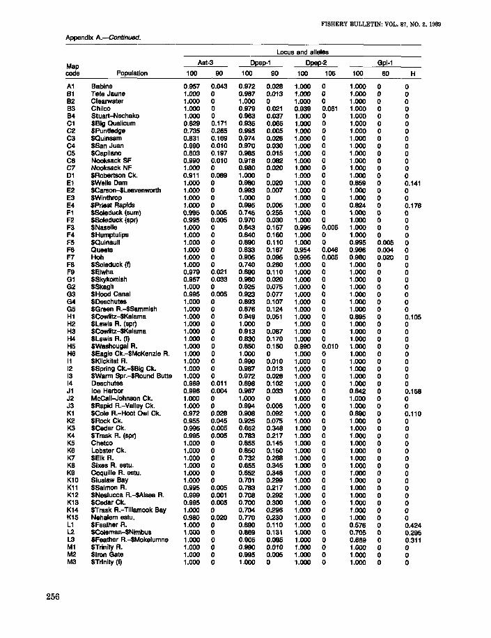
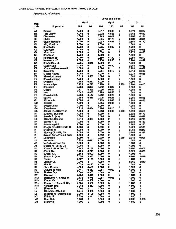
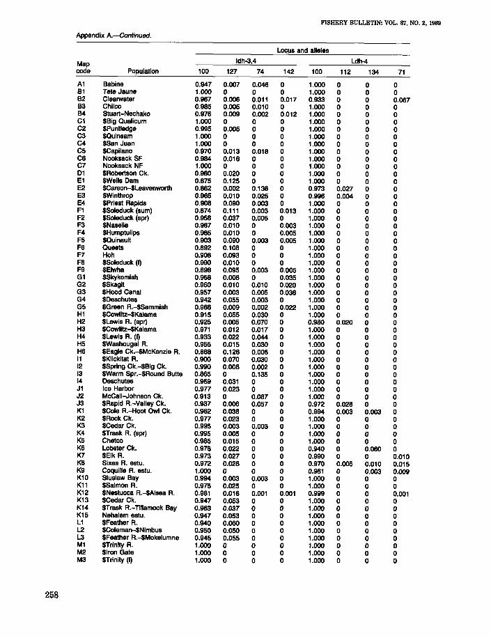
APPENDIX A

Allele frequencies and average heterozygosities for 65 individual and pooled populations ofnaturally reproducing and hatchery stocks of chinook salmon. Hatchery stocks are identifiedby ($). The map code refers to Figure 1.

254

UTl'ER ET AL.: GENETIC POPULATION STRUCTURE OF CHINOOK SALMON

Appendix A.--Continued.

Locus and alleles

MapAh Ada-1 Aat-1,2

code Population 100 86 116 108 69 100 83 100 85

A1 Babine 0.986 0.014 0 0 0 0.986 0.014 1.000 0B1 Tete Jaune 0.882 0.118 0 0 0 0.986 0.014 1.000 0B2 Clearwater 0.786 0.214 0 0 0 0.900 0.100 1.000 0B3 Chilco 0.922 0.078 0 0 0 0.969 0.031 1.000 0B4 Stuart-Nechako 0.958 0.042 0 0 0 0.894 0.106 1.000 0C1 $BIg Oualicum 0.838 0.162 0 0 0 0.953 0.047 1.000 0C2 $Puntledge 0.610 0.390 0 0 0 0.975 0.025 0.990 0.010C3 $Quinsam 0.366 0.829 0.005 0 0 0.995 0.005 0.997 0.003C4 $San Juan 0.820 0.160 0 0.020 0 1.000 0 0.987 0.013C5 $Capilano 0.763 0.237 0 0 0 0.909 0.091 0.967 0.033C6 Nooksack SF 0.780 0.220 0 0 0 0.870 0.130 0.995 0.005C7 Nooksack NF 0.810 0.190 0 0 0 0.927 0.073 0.922 0.07801 $Robertson Ck. 0.806 0.194 0 0 0 1.000 0 0.981 0.019E1 $Wells Dam 0.800 0.200 0 0 0 1.000 0 1.000 0E2 $Carson-$Leavenworth 0.987 0.010 0.003 0 0 0.969 0.031 1.000 0E3 $Winthrop 0.920 0.070 0.010 0 0 0.973 0.027 1.000 0E4 SPriest Rapids 0.825 0.175 0 0 0 0.985 0.015 1.000 0F1 $Soleduck (sum) 0.959 0.036 0.005 0 0 1.000 0 0.929 0.071F2 $Soleduck (spr) 0.848 0.152 0 0 0 0.995 0.005 0.998 0.003F3 $Naselle 0.908 0.092 0 0 0 0.980 0.020 0.965 0.035F4 $Humptulips 0.920 0.080 0 0 0 1.000 0 0.975 0.025F5 $Quinault 0.920 0.080 0 0 0 0.985 0.015 0.975 0.025F6 Queets 0.959 0.032 0.009 0 0 0.985 0.015 0.994 0.006F7 Hoh 0.930 0.040 0.030 0 0 1.000 0 0.994 0.006F8 $Soleduck (I) 0.837 0.133 0.031 0 0 1.000 0 1.000 0F9 $Elwha 0.920 0.060 0 0 0 0.980 0.020 1.000 0G1 $Skykomish 0.860 0.135 0.005 0 0 0.865 0.135 0.980 0.020G2 $Skagit 0.838 0.162 0 0 0 0.959 0.041 0.985 0.015G3 $Hood Canal 0.918 o.on 0.005 0 0 0.903 0.097 0.888 0.112G4 $Deschutes 0.842 0.158 0 0 0 0.953 0.047 0.913 0.088G5 $Green R.-$Sammish 0.903 0.097 0 0 0 0.973 0.027 0.966 0.034H1 $Cowlitz-$Kalama 0.845 0.149 0.006 0 0 0.975 0.025 1.000 0H2 $Lewis A. (spr) 0.910 0.060 0 0 0.010 0.980 0.020 0.995 0.005H3 $Cowlitz-$Kalama 0.855 0.131 0.014 0 0 0.993 0.007 1.000 0H4 $Lewis R. (I) 0.800 0.200 0 0 0 0.980 0.020 1.000 0H5 $Washougal A. 0.850 0.120 0.030 0 0 1.000 0 0.995 0.005H6 $Eagle Ck.-$McKenzie R. 0.782 0.190 0.029 0 0 1.000 0 1.000 011 $Klickitat R. 0.930 0.070 0 0 0 0.980 0.020 0.995 0.00512 $Spring Ck.-$Big Ck. 0.990 0.010 0 0 0 1.000 0 1.000 013 $Wa~m Spr.-$Round Butte 1.000 0 0 0 0 1.000 0 0.996 0.00414 Deschutes 0.867 0.102 0.031 0 0 0.990 0.010 1.000 0J1 Ice Harbor 0.874 0.111 0.003 0.013 0 0.998 0.003 1.000 0J2 McCall-Johnson Ck. 1.000 0 0 0 0 0.953 0.047 0.981 0.019J3 $Rapid R.-Valley Ck. 0.994 0.006 0 0 0 0.969 0.031 0.997 0.003K1 $Cole A.-Hoot Owl Ck. 0.957 0.043 0 0 0 1.000 0 0.998 0.002K2 $Rock Ck. 0.890 0.105 0.005 0 0 1.000 0 0.990 0.010K3 $Cedar Ck. 0.760 0.087 0.036 0.010 0.107 1.000 0 0.987 0.013K4 $Trask R. (spr) 0.735 0.110 0.020 0.020 0.115 1.000 0 0.978 0.023K5 Chetco 0.890 0.110 0 0 0 0.990 0.010 0.990 0.010K6 Lobster Ck. 0.930 0.070 0 0 0 1.000 0 0.975 0.025K7 $Elk R. 0.800 0.185 0.015 0 0 0.950 0.050 0.950 0.050K8 Sixes R. estu. 0.850 0.105 0.035 0.010 0 0.985 0.015 0.968 0.032K9 Coquille R. estu. 0.883 0.113 0 0.004 0 0.965 0.035 0.949 0.051K10 Siuslaw Bay 0.790 0.136 0.049 0.006 0.019 0.976 0.024 0.959 0.041K11 $Salmon R. 0.737 0.076 0.152 0.035 0 1.000 0 ,0.990 0.010K12 $Nestucca R.-$Alsea R. 0.811 0.064 0.113 0.001 0.012 0.969 0.031 0.976 0.024K13 $Cedar Ck. 0.610 0.215 0.120 0 0.055 0.995 0.005 0.944 0.056K14 $Trask R.-Tillamook Bay 0.730 0.141 0.113 0.003 0.013 0.968 0.032 0.991 0.009K15 Nehalem estu. 0.685 0.236 0.079 0 0 0.984 0.016 0.990 0.010L1 $Feather R. 0.720 0.240 0.040 0 0 1.000 0 1.000 0L2 $Coleman-$Nimbus 0.815 0.173 0.007 0.005 0 1.000 0 0.992 0.006L3 $Feather R.-$Mokelumne 0.797 0.195 0.005 0.002 0 1.000 0 0.999 0.001M1 $Trinity R. 1.000 0 0 0 0 1.000 0 1.000 0M2 $Iron Gate 0.995 0 0 0.005 0 1.000 0 0.997 0.003M3 $Trinity (I) 1.000 0 0 0 0 1.000 0 1.000 0

255

FISHERY BULLETIN: VOL. 87, NO.2. 1989

Appendix A.-Continued.

Locus and alleles

Map Aat-3 Dpep-1 Dpep-2 Gpi-1

code Population 100 90 100 90 100 105 100 60 H

A1 Babine 0.957 0.043 0.972 0.028 1.000 0 1.000 0 0B1 Tete Jaune 1.000 0 0.987 0.013 1.000 0 1.000 0 0B2 Clearwater 1.000 0 1.000 0 1.000 0 1.000 0 0B3 Chilco 1.000 0 0.979 0.021 0.939 0.061 1.000 0 0B4 Stuart-Nechako 1.000 0 0.963 0.037 1.000 0 1.000 0 0C1 $8ig Qualicum 0.829 0.171 0.935 0.065 1.000 0 1.000 0 0C2 $PunUedge 0.735 0.265 0.995 0.005 1.000 0 1.000 0 0C3 $Quinsam 0.831 0.169 0.974 0.026 1.000 0 1.000 0 0C4 $San Juan 0.990 0.010 0.970 0.030 1.000 0 1.000 0 0C5 $Capilano 0.803 0.197 0.985 0.015 1.000 0 1.000 0 0C6 Nooksack SF 0.990 0.010 0.918 0.082 1.000 0 1.000 0 0C7 Nooksack NF 1.000 0 0.980 0.020 1.000 0 1.000 0 001 $Robertson Ck. 0.911 0.089 1.000 0 1.000 0 1.000 0 0E1 $Wells Dam 1.000 0 0.980 0.020 1.000 0 0.859 0 0.141E2 $Carson-$Leavenworth 1.000 0 0.993 0.007 1.000 0 1.000 0 0E3 $Winthrop 1.000 0 1.000 0 1.000 0 1.000 0 0E4 SPriest Rapids 1.000 0 0.995 0.005 1.000 0 0.624 0 0.176F1 $SoIeduck (sum) 0.995 0.005 0.745 0.255 1.000 0 1.000 0 0F2 $Soleduck (spr) 0.995 0.005 0.970 0.030 1.000 0 1.000 0 0F3 $Naselle 1.000 0 0.843 0.157 0.995 0.005 1.000 0 0F4 $Humptulips 1.000 0 0.840 0.160 1.000 0 1.000 0 0F5 $Quinault 1.000 0 0.890 0.110 1.000 0 0.995 0.005 0F6 Queets 1.000 0 0.833 0.167 0.954 0.046 0.996 0.004 0F7 Hoh 1.000 0 0.905 0.095 0.995 0.005 0.980 0.020 0F8 SSoleduck (I) 1.000 0 0.740 0.280 1.000 0 1.000 0 0F9 $Elwha 0.979 0.021 0.890 0.110 1.000 0 1.000 0 0G1 $Skykomish 0.967 0.033 0.980 0.020 1.000 0 1.000 0 0G2 $Skagit 1.000 0 0.925 0.075 1.000 0 1.000 0 0G3 $Hoed Canal 0.995 0.005 0.923 0.077 1.000 0 1.000 0 0G4 $Deschutes 1.000 0 0.893 0.107 1.000 0 1.000 0 0G5 $Green A.-$Sammish 1.000 0 0.876 0.124 1.000 0 1.000 0 0H1 $Cowlitz-$Kalama 1.000 0 0.949 0.051 1.000 0 0.895 0 0.105H2 $Lewis A. (spr) 1.000 0 1.000 0 1.000 0 1.000 0 0H3 $Cowlitz-$Kalama 1.000 0 0.913 0.087 1.000 0 1.000 0 0H4 $Lewis R. (I) 1.000 0 0.830 0.170 1.000 0 1.000 0 0H5 $Washougal A. 1.000 0 0.850 0.150 0.990 0.010 1.000 0 0H6 $Eagle Ck.-$McKenzie R. 1.000 0 1.000 0 1.000 0 1.000 0 011 $Klickitat R. 1.000 0 0.990 0.010 1.000 0 1.000 0 012 $Spring Ck.-$Big Ck. 1.000 0 0.987 0.013 1.000 0 1.000 0 013 SWarm Spr.-$Round Butte 1.000 0 0.972 0.028 1.000 0 1.000 0 014 Deschutes 0.989 0.011 0.898 0.102 1.000 0 1.000 0 0J1 Ice Harbor 0.996 0.004 0.967 0.033 1.000 0 0.842 0 0.158J2 McCall-Johnson Ck. 1.000 0 1.000 0 1.000 0 1.000 0 0J3 $Rapid A.-Valley Ck. 1.000 0 0.994 0.006 1.000 0 1.000 0 0K1 $Cole A.-Hoot Owl Ck. 0.972 0.028 0.908 0.092 1.000 0 0.890 0 0.110K2 $Rock Ck. 0.955 0.045 0.925 0.075 1.000 0 1.000 0 0K3 $Cedar Ck. 0.995 0.005 0.652 0.348 1.000 0 1.000 0 0K4 $Trask R. (spr) 0.995 0.005 0.783 0.217 1.000 0 1.000 0 0K5 Chetco 1.000 0 0.855 0.145 1.000 0 1.000 0 0K6 Lobster Ck. 1.000 0 0.850 0.150 1.000 0 1.000 0 0K7 $Elk R. 1.000 0 0.732 0.268 1.000 0 1.000 0 0K8 Sixes A. estu. 1.000 0 0.655 0.345 1.000 0 1.000 0 0K9 Coquille R. estu. 1.000 0 0.652 0.348 1.000 0 1.000 0 0K10 Sluslaw Bay 1.000 0 0.701 0.299 1.000 0 1.000 0 0K11 $Salmon R. 0.995 0.005 0.783 0.217 1.000 0 1.000 0 0K12 $Nestucca A.-$Alsea A. 0.999 0.001 0.708 0.292 1.000 0 1.000 0 0K13 $Cedar Ck. 0.995 0.005 0.700 0.300 1.000 0 1.000 0 0K14 $Trask R.-Tillamook Bay 1.000 0 0.704 0.296 1.000 0 1.000 0 0K15 Nehalem estu. 0.980 0.020 o.no 0.230 1.000 0 1.000 0 0L1 $Feather R. 1.000 0 0.890 0.110 1.000 0 0.576 0 0.424L2 $CoIeman-$Nimbus 1.000 0 0.869 0.131 1.000 0 0.705 0 0.295L3 $Feather A.-$Mokelumne 1.000 0 0.905 0.095 1.000 0 0.689 0 0.311M1 $Trinily R. 1.000 0 0.990 0.010 1.000 0 1.000 0 0M2 $Iron Gate 1.000 0 0.995 0.005 1.000 0 1.000 0 0M3 $Trinily (I) 1.000 0 1.000 0 1.000 0 1.000 0 0

256

U'ITER ET AL.: GENETIC POPULATION STRUCTURE OF CHINOOK SALMON

Appendix A.-Continued.

Locus and alleles

Map Gpi-2 Gpi-3 Gr

code Population 100 60 100 105 93 100 85

A1 Babine 1.000 0 0.917 0.083 0 0.973 0.027B1 Tete Jaune 1.000 0 0.932 0.068 0 0.958 0.042B2 Clearwater 1.000 0 0.989 0.011 0 0.856 0.144B3 Chilco 1.000 0 0.875 0.125 0 0.939 0.061B4 Stuart-Nechako 1.000 0 0.933 0.067 0 0.860 0.140C1 $Big Qualicum 1.000 0 1.000 0 0 1.000 0C2 $Puntledge 1.000 0 0.995 0.005 0 1.000 0C3 $Quinsam 1.000 0 1.000 0 0 0.995 0.005C4 $San Juan 1.000 0 1.000 0 0 0.970 0.030C5 $Capilano 1.000 0 1.000 0 0 1.000 0C6 Nooksack SF 1.000 0 0.880 0.120 0 0.990 0.010C7 Nooksack NF 1.000 0 0.950 0.050 0 0.908 0.09201 $Robertson Ck. 0.755 0.245 1.000 0 0 1.000 0E1 $Wells Dam 1.000 0 0.970 0.030 0 0.980 0.020E2 $Carson-$Leavenworth 1.000 0 1.000 0 0 0.993 0.007E3 $Winthrop 1.000 0 0.984 0.016 0 0.918 0.082E4 SPriest Rapids 1.000 0 1.000 0 0 0.975 0.025F1 $Soleduck (sum) 0.613 0.387 1.000 0 0 1.000 0F2 $Soleduck (spr) 1.000 0 1.000 0 0 1.000 0F3 $Naselle 0.788 0.212 1.000 0 0 1.000 0F4 $Humptulips 0.755 0.245 0.970 0 0.030 0.990 0.010F5 $Quinault 0.700 0.300 0.980 0.020 0 1.000 0F6 Queets 0.671 0.329 0.996 0.004 0 1.000 0F7 Hoh 0.542 0.458 0.995 0.005 0 1.000 0F8 $Soleduck (I) 0.553 0.447 0.980 0.020 0 1.000 0F9 $Elwha 0.684 0.316 0.975 0.025 0 0.995 0.005G1 $Skykomish 1.000 0 0.955 0.045 0 0.995 0.005G2 $Skagit 1.000 0 0.995 0.005 0 1.000 0G3 $Hood Canal 1.000 0 1.000 0 0 1.000 0G4 $Deschutes 0.916 0.084 0.990 0.010 0 1.000 0G5 $Green R.-$Sammish 1.000 0 0.993 0.003 0.003 0.990 0.010H1 $Cowlitz-$Kalama 1.000 0 1.000 0 0 0.822 0.179H2 $Lewis R. (spr) 1.000 0 1.000 0 0 0.908 0.092H3 $Cowlitz-$Kalama 0.916 0.084 1.000 0 0 0.795 0.205H4 $Lewis A. (I) 1.000 0 1.000 0 0 0.820 0.180H5 $Washougal R. 1.000 0 1.000 0 0 0.800 0.200H6 $Eagle Ck.-$McKenzie A. 1.000 0 1.000 0 0 0.420 0.58011 $Klickitat A. 1.000 0 1.000 0 0 0.760 0.24012 $Spring Ck.-$Big Ck. 1.000 0 1.000 0 0 0.663 0.33713 SWarm Spr.-$Round Bulle 1.000 0 1.000 0 0 1.000 014 Deschutes 1.000 0 0.990 0 0.010 0.949 0.051J1 Ice Harbor 0.929 0.071 1.000 0 0 1.000 0J2 McCall-Johnson Ck. 1.000 0 1.000 0 0 1.000 0J3 $Rapid A.-Valley Ck. 1.000 0 1.000 0 0 1.000 0K1 $Cole R.-Hoot Owl Ck. 0.842 0.158 1.000 0 0 0.997 0.003K2 $Rock Ck. 0.755 0.245 1.000 0 0 0.925 0.075K3 $Cedar Ck. 0.698 0.302 1.000 0 0 1.000 0K4 $Trask A. (spr) 0.553 0.447 1.000 0 0 0.961 0.039K5 Chetco 0.827 0.173 1.000 0 0 1.000 0K6 Lobster Ck. 1.000 0 1.000 0 0 0.960 0.040K7 $Elk R. 0.520 0.480 1.000 0 0 1.000 0K8 Sixes A. estu. 0.434 0.566 1.000 0 0 1.000 0K9 Coquille A. estu. 0.441 0.559 0.991 0.009 0 1.000 0K10 Siuslaw Bay 0.545 0.455 1.000 0 0 1.000 0K11 $Salmon A. 0.682 0.318 1.000 0 0 1.000 0K12 $Nestucca A.-$Alsea A. 0.525 0.475 0.997 0.003 0 1.000 01(13 $Cedar Ck. 0.432 0.568 1.000 0 0 1.000 0K14 $Trask A.-Tillamook Bay 0.435 0.565 1.000 0 0 1.000 0K15 Nehalem estu. 0.783 0.217 1.000 0 0 1.000 0L1 $Feather A. 1.000 0 1.000 0 0 1.000 0L2 $Coleman-$Nimbus 0.945 0.055 1.000 0 0 1.000 0L3 $Feather R.-$Mokelumne 0.900 0.100 1.000 0 0 1.000 0M1 $Trinity A. 0.859 0.141 1.000 0 0 1.000 0M2 $Iron Gate 1.000 0 1.000 0 0 0.995 0.005M3 $Trinity (I) 1.000 0 1.000 0 0 1.000 0

257

FISHERY BULLETIN: VOL. 87, NO.2, 1989

Appendix A.-Continued.

Locus and alleles

Map Idh-3,4 Ldh-4

code Population 100 127 74 142 100 112 134 71

A1 Babine 0.947 0.007 0.046 0 1.000 0 0 0B1 Tete Jaune 1.000 0 0 0 1.000 0 0 0B2 Clearwater 0.967 0.006 0.011 0.017 0.933 0 0 0.067B3 Chilco 0.985 0.005 0.010 0 1.000 0 0 0B4 Stuart-Nechako 0.976 0.009 0.002 0.012 1.000 0 0 0C1 $Big Qualicum 1.000 0 0 0 1.000 0 0 0C2 $Puntledge 0.995 0.005 0 0 1.000 0 0 0C3 $Quinsam 1.000 0 0 0 1.000 0 0 0C4 $San Juan 1.000 0 0 0 1.000 0 0 0C5 $Capilano 0.970 0.013 0.018 0 1.000 0 0 0C6 Nooksack SF 0.984 0.016 0 0 1.000 0 0 0C7 Nooksack NF 1.000 0 0 0 1.000 0 0 001 $Robertson Ck. 0.980 0.020 0 0 1.000 0 0 0E1 $Wells Dam 0.875 0.125 0 0 1.000 0 0 0E2 $Carson-$Leavenworth 0.862 0.002 0.136 0 0.973 0.027 0 0E3 $Winthrop 0.965 0.010 0.025 0 0.996 0.004 0 0E4 SPriest Rapids 0.908 0.090 0.003 0 1.000 0 0 0F1 $Soleduck (sum) 0.874 0.111 0.003 0.013 1.000 0 0 0F2 $Soleduck (spr) 0.958 0.037 0.005 0 1.000 0 0 0F3 $Naselle 0.987 0.010 0 0.003 1.000 0 0 0F4 $Humptulips 0.985 0.010 0 0.005 1.000 0 0 0F5 $Quinault 0.903 0.090 0.003 0.005 1.000 0 0 0F6 Queets 0.892 0.108 0 0 1.000 0 0 0F7 Hoh 0.906 0.093 0 0 1.000 0 0 0F8 $Soleduck (I) 0.990 0.010 0 0 1.000 0 0 0F9 $Elwha 0.898 0.095 0.003 0.005 1.000 0 0 0G1 $Skykomish 0.958 0.006 0 0.035 1.000 0 0 0G2 $Skagit 0.960 0.010 0.010 0.020 1.000 0 0 0G3 $Hood Canal 0.957 0.003 0.005 0.036 1.000 0 0 0G4 $Deschutes 0.942 0.055 0.003 0 1.000 0 0 0G5 $Green A.-$Sammish 0.968 0.009 0.002 0.022 1.000 0 0 0H1 $Cowlitz-$Kalama 0.915 0.055 0.030 0 1.000 0 0 0H2 $Lewis R. (spr) 0.925 0.005 0.070 0 0.980 0.020 0 0H3 $Cowlitz-$Kalama 0.971 0.012 0.017 0 1.000 0 0 0H4 $Lewis R. (I) 0.933 0.022 0.044 0 1.000 0 0 0H5 $Washougal A. 0.955 0.015 0.030 0 1.000 0 0 0H6 $Eagle Ck.-$McKenzie A. 0.868 0.126 0.006 0 1.000 0 0 011 $Klickitat A. 0.900 0.070 0.030 0 1.000 0 0 012 $Spring Ck.-$Big Ck. 0.990 0.008 0.002 0 1.000 0 0 013 SWarm Spr.-$Round Bulle 0.865 0 0.135 0 1.000 0 0 014 Deschutes 0.969 0.031 0 0 1.000 0 0 0J1 Ice Harbor 0.977 0.023 0 0 1.000 0 0 0J2 McCall-Johnson Ck. 0.913 0 0.087 0 1.000 0 0 0J3 $Rapid R.-Valley Ck. 0.937 0.006 0.057 0 0.972 0.028 0 0K1 $Cole A.-Hoot Owl Ck. 0.962 0.038 0 0 0.994 0.003 0.003 0K2 $Rock Ck. 0.977 0.023 0 0 1.000 0 0 0K3 $Cedar Ck. 0.995 0.003 0.003 0 1.000 0 0 0K4 $Trask R. (spr) 0.995 0.005 0 0 1.000 0 0 0K5 Chetco 0.965 0.015 0 0 1.000 0 0 0K6 Lobster Ck. 0.978 0.022 0 0 0.940 0 0.060 0K7 $Elk A. 0.973 0.027 0 0 0.990 0 0 0.010K8 Sixes R. estu. 0.972 0.028 0 0 0.970 0.005 0.010 0.015K9 Coquille A. estu. 1.000 0 0 0 0.961 0 0.003 0.009K10 Siuslaw Bay 0.994 0.003 0.003 0 1.000 0 0 0K11 $Salmon R. 0.975 0.025 0 0 1.000 0 0 0K12 $Nestucca A.-$Alsea A. 0.981 0.016 0.001 0.001 0.999 0 0 0.001K13 $Cedar Ck. 0.947 0.053 0 0 1.000 0 0 0K14 $Trask R.-Tillamook Bay 0.963 0.037 0 0 1.000 0 0 0K15 Nehalem estu. 0.947 0.053 0 0 1.000 0 0 0L1 $Feather A. 0.940 0.060 0 0 1.000 0 0 0L2 $Coleman-$Nimbus 0.950 0.050 0 0 1.000 0 0 0L3 $Feather R.-$Mokelumne 0.945 0.055 0 0 1.000 0 0 0M1 $Trinity A. 1.000 0 0 0 1.000 0 0 0M2 $Iron Gate 1.000 0 0 0 1.000 0 0 0M3 $Trinity (I) 1.000 0 0 0 1.000 0 0 0

258

UTl'ER ET AL.: GENETIC POPULATION STRUCTURE OF CHINOOK SALMON

ApPENDIX A.-Continued.

Locus and alleles

MapLdh-5 Mdh-1,2 Mdh-3,4

code Population 100 90 70 100 120 27 100 121 70 83

A1 Babine 1.000 0 0 1.000 0 0 1.000 0 0 0B1 Tete Jaune 1.000 0 0 1.000 0 0 1.000 0 0 0B2 Clearwater 1.000 0 0 1.000 0 0 0.989 0.006 0.006 0B3 Chilco 1.000 0 0 1.000 0 0 0.990 0 0.010 0B4 Stuart-Nechako 1.000 0 0 1.000 0 0 0.936 0 0.064 0C1 $BIg Qualicum 1.000 0 0 1.000 0 0 1.000 0 0 0C2 $Puntledge 1.000 0 0 1.000 0 0 0.948 0.037 0.015 0C3 $Quinsam 0.966 0.034 0 1.000 0 0 0.843 0.103 0.054 0C4 $San Juan 1.000 0 0 1.000 0 0 0.990 0.010 0 0C5 $Capilano 0.995 0.005 0 1.000 0 0 1.000 0 0 0C6 Nooksack SF 1.000 0 0 1.000 0 0 0.965 0.030 0.005 0C7 Nooksack NF 1.000 0 0 1.000 0 0 0.965 0 0.035 0D1 $Robertson Ck. 1.000 0 0 1.000 0 0 0.993 0.008 0 0E1 $Wells Dam 0.980 0.020 0 1.000 0 0 0.970 0.010 0.020 0E2 $Carson-$Leavenworth 1.000 0 0 1.000 0 0 0.978 0.022 0 0E3 $Winthrop 1.000 0 0 1.000 0 0 0.990 0.010 0 0E4 SPriest Rapids 0.964 0.015 0.020 1.000 0 0 0.955 0.030 0.015 0F1 $Soleduck (sum) 1.000 0 0 1.000 0 0 0.963 0.003 0.035 0F2 $Soleduck (spr) 1.000 0 0 1.000 0 0 0.975 0.015 0.010 0F3 $Naselle 1.000 0 0 1.000 0 0 0.944 0.040 0.015 0F4 $Humptulips 1.000 0 0 1.000 0 0 0.985 0.015 0 0F5 $Quinault 1.000 0 0 1.000 0 0 0.988 0.013 0 0F6 Queets 1.000 0 0 1.000 0 0 0.963 0.037 0 0F7 Hoh 1.000 0 0 1.000 0 0 0.993 0.003 0.003 0.003F8 $Soleduck (f) 1.000 0 0 1.000 0 0 0.985 0.015 0 0F9 $Elwha 1.000 0 0 1.000 0 0 0.968 0.015 0.017" 0G1 $Skykomish 0.980 0.020 0 1.000 0 0 0.990 0 0.010 0G2 $Skagit 0.990 0.010 0 1.000 0 0 0.993 0 0.008 0G3 $Hood Canal 1.000 0 0 1.000 0 0 0.967 0 0.033 0G4 $Deschutes 1.000 0 0 1.000 0 0 0.992 0 0.008 0G5 $Green R.-$Sammish 0.990 0.010 0 1.000 0 0 0.991 0.003 0.005 0H1 $Cowlitz-$Kalama 1.000 0 0 1.000 0 0 0.988 0.013 0 0H2 $Lewis R. (spr) 0.990 0.010 0 1.000 0 0 0.965 0.035 0 0H3 $Cowlitz-$Kalama 0.997 0.003 0 1.000 0 0 0.983 0.017 0 0H4 $Lewis R. (f) 1.000 0 0 1.000 0 0 1.000 0 0 0H5 $Washougal R. 1.000 0 0 1.000 0 0 0.990 0.010 0 0H6 $Eagle Ck.-$McKenzie R. 1.000 0 0 1.000 0 0 0.963 0.037 0 011 $Klickitat R. 1.000 0 0 1.000 0 0 0.970 0.030 0 012 $Spring Ck.-$Big Ck. 1.000 0 0 1.000 0 0 0.945 0.055 0 013 SWarm Spr.-$Round Butte 1.000 0 0 0.995 0.005 0 1.000 0 0 014 Deschutes 1.000 0 0 1.000 0 0 0.985 0.010 0.005 0J1 Ice Harbor 0.995 0.003 0.003 1.000 0 0 0.985 0.005 0.010 0J2 McCall-Johnson Ck. 0.976 0.024 0 1.000 0 0 0.998 0.002 0 0J3 $Rapid R.-Valley Ck. 1.000 0 0 1.000 0 0 0.995 0.005 0 0K1 $Cole R.-Hoot Owl Ck. 0.988 0.012 0 0.989 0 0.011 0.992 0.008 0 0K2 $Rock Ck. 1.000 0 0 1.000 0 0 0.968 0.030 0.003 0K3 $Cedar Ck. 0.975 0.025 0 1.000 0 0 0.995 0.005 0 0K4 $Trask R. (spr) 0.985 0.015 0 1.000 0 0 0.990 0.010 0 0K5 Chetco 1.000 0 0 0.998 0.003 0 0.955 0.045 0 0K6 Lobster Ck. 1.000 0 0 1.000 0 0 0.975 0.025 0 0K7 $Elk R. 1.000 0 0 0.998 0 0.003 0.983 0.017 0 0K8 Sixes R. estu. 1.000 0 0 0.945 0.027 0.027 0.993 0.008 0 0K9 Coquille R. estu. 0.996 0.004 0 0.987 0.011 0.002 0.996 0.004 0 0K10 Siuslaw Bay 0.982 0.018 0 0.997 0.003 0 0.982 0.018 0 0K11 $Salmon R. 1.000 0 0 1.000 0 0 1.000 0 0 0K12 $Nestucca R.-$Alsea R. 0.999 0.001 0 0.999 0.001 0 1.000 0 0 0K13 $Cedar Ck. 1.000 0 0 1.000 0 0 1.000 0 0 0K14 $Trask R.-Tillamook Bay 1.000 0 0 0.999 0.001 0 0.985 0.015 0 0K15 Nehalem estu. 1.000 0 0 1.000 0 0 1.000 0 0 0L1 $Feather R. 1.000 0 0 1.000 0 0 0.945' 0.055 0 0L2 $Coleman-$Nimbus 1.000 0 0 1.000 0 0 0.968 0.032 0 0L3 $Feather R.-$Mokelumne 1.000 0 0 1.000 0 0 0.9n 0.023 0 0M1 $Trinity R. 1.000 0 0 1.000 0 0 1.000 0 0 0M2 $Iron Gate 1.000 0 0 1.000 0 0 0.997 0.003 0 0M3 $Trinity (f) 1.000 0 0 1.000 0 0 1.000 0 0 0

259

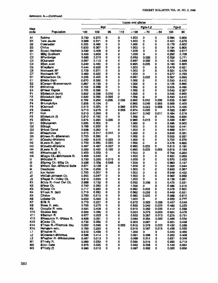
FISHERY BULLETIN: VOL. 87, NO.2, 1989

ApPENDIX A.-Gontinued.

Locus and alleles

MapMpi Pgm-1,2 Pgk-2

code Population 100 109 95 113 -100 -70 -84 100 90

A1 Babine 0.730 0.270 0 0 1.000 0 0 0.095 0.905B1 Tete Jaune 0.689 0.311 0 0 1.000 0 0 0.421 0.579B2 Clearwater 0.535 0.465 0 0 1.000 0 0 0.178 0.822B3 Chilco 0.633 0.367 0 0 1.000 0 0 0.194 0.806B4 Stuart-Nechako 0.592 0.408 0 0 1.000 0 0 0.383 0.617C1 $8ig Qualicum 0.400 0.800 0 0 1.000 0 0 0.292 0.708C2 $Puntledge 0.690 0.310 0 0 0.980 0.020 0 0.229 0.771C3 $Quinsam 0.887 0.113 0 0 0.997 0.002 0 0.151 0.849C4 $San Juan 0.540 0.460 0 0 0.995 0.005 0 0.180 0.820C5 $Capilano 0.444 0.556 0 0 1.000 0 0 0.479 0.521C6 Nooksack SF 0.729 0.271 0 0 1.000 0 0 0.521 0.479C7 Nooksack NF 0.480 0.520 0 0 1.000 0 0 0.277 0.72301 $Robertson Ck. 0.595 0.405 0 0 0.997 0.002 0 0.307 0.693E1 $Wells Dam 0.670 0.330 0 0 1.000 0 0 0.590 0.410E2 $Carson-$Leavenworth 0.867 0.133 0 0 1.000 0 0 0.105 0.895E3 $Winthrop 0.702 0.298 0 0 1.000 0 0 0.505 0.495E4 SPriest Rapids 0.705 0.295 0 0 1.000 0 0 0.643 0.357F1 $Soleduck (sum) 0.652 0.338 0.010 0 1.000 0 0 0.345 0.655F2 $Soleduck (spr) 0.630 0.365 0.005 0 1.000 0 0 0.490 0.510F3 $Naselle 0.709 0.250 0.005 0.036 0.982 0.012 0.005 0.638 0.362F4 $Humptulips 0.806 0.194 0 0 0.950 0.045 0.005 0.600 0.400F5 $Quinault 0.613 0.325 0 0.062 0.970 0.023 0.008 0.575 0.425F6 Queets 0.713 0.279 0 0.008 0.974 0.025 0 0.333 0.667F7 Hoh 0.610 0.390 0 0 0.947 0.042 0.011 0.484 0.516F8 $Soleduck (f) 0.810 0.190 0 0 1.000 0 0 0.365 0.635F9 $Elwha 0.675 0.290 0.035 0 0.985 0.015 0 0.399 0.801G1 $Skykomish 0.695 0.305 0 0 1.000 0 0 0.495 0.505G2 $Skagit 0.768 0.232 0 0 1.000 0 0 0.559 0.441G3 $Hood Canal 0.608 0.392 0 0 1.000 0 0 0.689 0.311G4 $Deschutes 0.673 0.317 0.010 0 1.000 0 0 0.649 0.351G5 $Green R.-$Sammish 0.720 0.280 0 0 1.000 0 0 0.663 0.337H1 $Cowlitz-$Kalama 0.460 0.515 0.025 0 1.000 0 0 0.722 0.278H2 $Lewis R. (spr) 0.700 0.280 0.020 0 1.000 0 0 0.378 0.622H3 $Cowlitz-$Kalama 0.467 0.497 0.037 0 0.995 0.005 0 0.810 0.190H4 $Lewis R. (f) 0.380 0.490 0.130 0 0.990 0.005 0.005 0.816 0.184H5 $Washougal A. 0.450 0.550 0 0 1.000 0 0 0.750 0.250H6 $Eagle Ck.-$McKenzie A. 0.458 0.542 0 0 1.000 0 0 0.931 0.06911 $Klickitat A. 0.730 0.260 0.010 0 1.000 0 0 0.570 0.43012 $Spring Ck.-$Big Ck. 0.596 0.356 0.048 0 1.000 0 0 0.863 0.13713 SWarm Spr.-$Round Butte 0.871 0.129 0 0 1.000 0 0 0.356 0.64414 Deschutes 0.704 0.296 0 0 1.000 0 0 0.633 0.367J1 Ice Harbor 0.793 0.207 0 0 1.000 0 0 0.548 0.452J2 McCall-Johnson Ck. 0.953 0.047 0 0 1.000 0 0 0.062 0.938J3 $Rapid A.-Valley Ck. 0.910 0.090 0 0 1.000 0 0 0.139 0.861K1 $Cole R.-Hoot Owl Ck. 0.868 0.132 0 0 0.992 0.008 0 0.470 0.531K2 $Rock Ck. 0.740 0.260 0 0 1.000 0 0 0.485 0.515K3 $Cedar Ck. 0.717 0.283 0 0 0.992 0.008 0 0.378 0.622K4 $Trask A. (spr) 0.710 0.290 0 0 0.962 0.038 0 0.449 0.551K5 Chetco 0.790 0.210 0 0 0.980 0.020 0 0.388 0.612K6 Lobster Ck. 0.550 0.450 0 0 1.000 0 0 0.223 0.777K7 $Elk R. 0.773 0.227 0 0 0.972 0.023 0.005 0.457 0.543K8 Sixes R. estu. 0.725 0.275 0 0 0.938 0.040 0.023 0.480 0.520K9 Coquille A. estu. 0.591 0.409 0 0 0.915 0.050 0.035 0.412 0.568K10 Siuslaw Bay 0.605 0.395 0 0 0.924 0.073 0.003 0.524 0.476K11 $Salmon A. 0.677 0.323 0 0 0.920 0.067 0.013 0.279 0.721K12 $Nestucca R.-SAlsea A. 0.639 0.361 0 0 0.944 0.054 0.002 0.466 0.534K13 $Cedar Ck. 0.735 0.265 0 0 0.903 0.097 0 0.551 0.449K14 $Trask A.-Tillamook Bay 0.652 0.346 0 0.003 0.918 0.079 0.003 0.432 0.568K15 Nehalem estu. 0.780 0.220 0 0 0.918 0.067 0.015 0.438 0.563L1 $Feather A. 0.510 0.490 0 0 1.000 0 0 0.540 0.460L2 $Coleman-$Nimbus 0.586 0.414 0 0 0.991 0.009 0 0.592 0.408L3 $Feather R.-$Mokelumne 0.487 0.513 0 0 0.988 0.011 0 0.651 0.349M1 $Trinity R. 0.980 0.020 0 0 0.985 0.015 0 0.290 0.710M2 $Iron Gate 0.975 0.025 0 0 0.942 0.058 0 0.146 0.854M3 $Trinity (f) 0.990 0.010 0 0 0.997 0.002 0 0.350 0.650

260

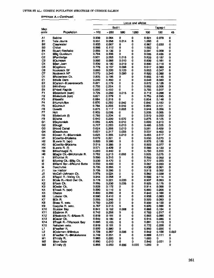
UTTER ET AL.: GENETIC POPULATION STRUCTURE OF CHINOOK SALMON

ApPENDIX A.-Continued.

L.ocus and alleles

Map Sod·1 Tapep-1

code Population -100 -260 580 1260 100 130 45

A1 Babine 0.936 0.064 0 0 0.921 0.079 0B1 Tete Jaune 0.931 0.056 0.014 0 1.000 0 0B2 Clearwater 0.933 0.067 0 0 0.967 0.033 0B3 Chilco 0.888 0.112 0 0 1.000 0 0B4 Stuart-Nechako 0.865 0.135 0 0 0.991 0.009 0C1 $Big Qualicum 0.794 0.206 0 0 0.565 0.435 0C2 $Puntledge 0.931 0.053 0.016 0 0.803 0.197 0C3 $Quinsam 0.892 0.098 0.010 0 0.839 0.161 0C4 $San Juan 0.800 0.190 0.010 0 0.890 0.110 0C5 $Capilano 0.778 0.157 0.066 0 0.617 0.383 0C6 Nooksack SF 0.660 0.220 0.120 0 0.653 0.347 0C7 Nooksack NF 0.570 0.340 0.090 0 0.620 0.380 001 $Robertson Ck. 0.805 0.195 0 0 0.655 0.145 0E1 $Wells Dam 0.540 0.460 0 0 0.640 0.360 0E2 $Ca~on-$Leavenworth 0.821 0.179 0 0 0.872 0.128 0E3 $Winthrop 0.736 0.264 0 0 0.992 0.008 0E4 SPriest Rapids 0.550 0.450 0 0 0.793 0.207 0F1 $Soleduck (sum) 0.725 0.260 0.015 0 0.712 0.288 0F2 $Soleduck (spr) 0.621 0.379 0 0 0.755 0.245 0F3 $Naselle 0.684 0.316 0 0 0.854 0.146 0F4 $Humptulips 0.670 0.290 0.040 0 0.840 0.160 0F5 $Quinault 0.784 0.206 0.010 0 0.899 0.101 0F6 Queets 0.875 0.117 0.008 0 0.944 0.056 0F7 Hoh 0.905 0.095 0 0 0.935 0.065 0F8 $Soleduck (I) 0.796 0.204 0 0 0.970 0.030 0F9 $Elwha 0.640 0.290 0.070 0 0.875 0.125 0G1 $Skykomish 0.565 0.425 0.010 0 0.690 0.310 0G2 $Skagit 0.707 0.283 0.010 0 0.495 0.505 0G3 $Hood Canal 0.624 0.366 0.010 0 0.561 0.439 0G4 $Deschutes 0.627 0.317 0.056 0 0.507 0.493 0G5 $Green R.-$Sammish 0.625 0.365 0.010 0 0.483 0.517 0H1 $Cowlilz-$Kalama 0.679 0.321 0 0 0.930 0.070 0H2 $Lewis R. (spr) 0.620 0.380 0 0 0.875 0.125 0H3 $Cowlilz-$Kalama 0.615 0.385 0 0 0.923 o.on 0H4 $Lewis R. (I) 0.571 0.429 0 0 0.880 0.120 0H5 $Washougal R. 0.560 0.440 0 0 0.780 0.220 0H6 $Eagle Ck.-$McKenzie R. 0.782 0.213 0.006 0 0.925 0.075 011 $Klickitat R. 0.690 0.310 0 0 0.950 0.050 012 $Spring Ck.-$Big Ck. 0.530 0.470 0 0 0.777 0.223 013 SWarm Spr.-$Round Butte 0.550 0.450 0 0 0.967 0.033 014 Deschutes 0.735 0.265 0 0 0.939 0.061 0J1 Ice Harbor 0.705 0.295 0 0 0.918 0.082 0J2 McCall-Johnson Ck. 0.976 0.024 0 0 0.962 0.038 0J3 $Rapid R.-Valley Ck. 0.944 0.056 0 0 0.886 0.114 0K1 $Cole R.-Hoot Owl Ck. 0.n6 0.221 0.003 0 0.937 0.063 0K2 $Rock Ck. 0.665 0.330 0.005 0 0.825 0.175 0K3 $Cedar Ck. 0.828 0.172 0 0 0.914 0.086 0K4 $Trask R. (spr) 0.890 0.110 0 0 0.800 0.200 0K5 Chetco 0.800 0.200 0 0 0.840 0.160 0K6 L.obster Ck. 0.590 0.410 0 0 0.938 0.063 0K7 $Elk R. 0.655 0.345 0 0 0.920 0.080 0K8 Sixes R. estu. 0.780 0.220 0 0 0.900 0.100 0K9 Coquille R. estu. 0.787 0.213 0 0 0.920 0.080 0K10 Siuslaw Bay 0.841 0.152 0.006 0 0.866 0.134 0K11 $Salmon R. 0.742 0.258 0 0 0.783 0.217 0K12 $Nestucca R.-$Alsea R. 0.819 0.181 0 0 0.905 0.095 0K13 $Cedar Ck. 0.840 0.160 0 0 0.915 0.085 0K14 $Trask R.-Tillamook Bay 0.895 0.105 0 0 0.881 0.119 0K15 Nehalem estu. 0.819 0.181 0 0 0.772 0.228 0L1 $Feather R. 0.620 0.380 0 0 0.950 0.050 0L2 $Coleman-$Nimbus 0.728 0.267 0.005 0 0.842 0.156 0.002L3 $Feather R.-$Mokelumne 0.749 0.251 0 0 0.889 0.111 0M1 $Trinity R. 0.980 0.020 0 0 1.000 0 0M2 $Iron Gate 0.990 0.010 0 0 0.949 0.051 0M3 $Trinily (I) 0.895 0.050 0.035 0.020 1.000 0 0

261

262

FISHERY BULLETIN: VOL. 87, NO.2, 1989

ApPENDIX A.-Continued.

Map Dendrogram Populationcode Population Heterozygosity cluster unit

A1 Babine 0.057 5A 1B1 Tete Jaune 0.061 5A 1B2 Clearwater 0.082 5A 1B3 Chilco 0.071 5A 1B4 Stuart-Nechako 0.090 5A 1Cl $Big Qualicum 0.099 6 2C2 $Puntledge 0.101 3 2C3 $Quinsam 0.095 3 2C4 $San Juan 0.074 5A 2C5 SCapilano 0.118 6 2C6 Nooksack SF 0.122 8E 3C7 Nooksack NF 0.124 6 201 $Robertson Ck. 0.105 4 4El $Wells Dam 0.127 8E 6E2 $Carson-SLeavenworth 0.067 5B 6E3 $Winthrop 0.076 8C 6E4 SPriest Rapids 0.118 8E 6F1 $SOleduck (sum) 0.141 4 4F2 $So/educk (spr) 0.097 BE 4F3 $Naselle 0.114 8B 4F4 $Humptulips 0.112 8B 4F5 $Quinault 0.119 4 4F6 Queets 0.111 4 4F7 Hoh 0.109 4 4F8 SSoleduck (f) 0.098 4 4F9 SElwha 0.125 8B 4Gl SSkykomish 0.114 8E 3G2 $Skagit 0.101 80 3G3 SHood Canal 0.122 80 3G4 $Deschutes 0.128 80 3G5 $Green A.-$Sammish 0.105 80 3Hl SCowlitz-$Kalama 0.110 2 5H2 SLewis A. (spr) 0.113 8C 6H3 SCowlitz-$Kalama 0.103 2 5H4 $Lewis A. (f) 0.113 2 5H5 $Washougal A. 0.112 2 5H6 SEagle Ck.-$McKenzie R. 0.102 1 511 $Klickitat R. 0.099 8C 612 $Spring Ck.-$Big Ck. 0.093 2 513 SWarm Spr.-$Round Butte 0.072 SA 614 Deschutes 0.086 8C 6Jl Ice Harbor 0.090 8B 6J2 McCall-Johnson Ck. 0.035 5B 7J3 $Rapid A.-Valley Ck. 0.045 5B 7Kl SCole R.-Hoot Owl Ck. 0.090 8B 4K2 SRock Ck. 0.112 8B 4K3 $Cedar Ck. 0.111 4 4K4 STrask R. (spr) 0.124 4 4K5 Chetco 0.100 8B 4K6 Lobster Ck. 0.092 5A 4K7 $Elk R. 0.130 4 4K8 Sixes A. estu. 0.137 4 4K9 Coquille R. estu. 0.134 4 4K10 Siuslaw Bay 0.135 4 4K11 $Salmon R. 0.128 4 4K12 $Nestucca R.-$Alsea A. 0.125 4 4K13 SCedar Ck. 0.143 4 4K14 $Trask A.-Tillamook Bay 0.132 4 4K15 Nehalem estu. 0.131 4 4Ll SFeather R. 0.124 7 9L2 SColeman-$Nimbus 0.123 7 9L3 SFeather R.-$Mokelumne 0.119 7 9Ml $Trinity A. 0.032 5B 8M2 $Iron Gate 0.027 5B 8M3 STrinity (f) 0.027 5B 8

UTIER ET AL.: GENETIC POPULATION STRUCTURE OF CHINOOK SALMON

APPENDIX B

Previously Unreported Genetic Variants

Glutathione reductase (Gr) was the more readilyinterpreted of the two previously undescribed poly­morphic enzymes observed for chinook salmon inthis study. The phenotypic forms (App. Fig. 1) werethose expected from a dimeric enzyme with threealleles and were consistent with known allelicvariants of Gr observed in other vertebrates (e.g.,man) (Harris and Hopkinson 1976). The assumptionthat this variation was a three-allele polymorphismwas supported by the conformance of phenotypicratios to those expected under Hardy-Weinbergequilibrium, the absolute repeatability of expressionfrom independent extractions, and the parallelexpression of different tissues (eye and skeletal mus­cle) from individuals expressing a given phenotype.

The previously undescribed glucose-6-phosphateisomerase (Gpi) variation was less readily explained.Individuals homozygous for the common alleles ateach of the three Gpi loci express a six-bandedphenotype that is directly interpreted as havingthree homodimeric and three heterodimeric bands(App. Fig. 2). An extension of this interpretationalso explains additional numbers of bands whicharise from allelic forms having different mobilities,or fewer bands resulting from either allelic formsof different loci having common mobilities or fromnull alleles. However, none of these explanationsadequately describe the five-banded Gpi phenotypes

that have been found with regularity in somecollections.

One explanation that is consistent with the ob­served phenotypes is that the subunits encoded bya locus aggregate randomly, but that the aggrega­tions for some interlocus combinations are pre­cluded. Such inhibited combinations are commonamong duplicated loci of salmonids. For instance,subunits of Ldh-3 and Ldh-5 randomly aggregate.as do those of Ldh-3 and Ldh-4; however. Ldh-4 andLdh-5 subunits do not aggregate (Wright et al.1975). Mutations precluding aggregation (but notnecessarily affecting electrophoretic mobility) musthave arisen at some time between the duplicationevent and the present, and such mutations musthave been polymorphic between their arising andtheir fixation (see Allendorf and Thorgaard 1984,for a review of gene duplication in salmonids).

The above model was tested when gametes andtissues were obtained from individuals of the PriestRapids stock where five-banded Gpi phenotypeswere commonly observed. Because of difficulty inunambiguously discerning common and presumedheterozygous phenotypes. the only informativecrosses were those involving the single parent hav­ing a five-banded phenotype. The phenotypic ratiosof the two matings involving this individual (App.Table 1) conform to those expected from a Men-

+

Samplenumber 12345 678 9 10 11 12 13 14 15 16 17 18 19

ApPENDIX FIGURE I.-Glutathione reductase phenotypes of chinook salmon from eye fluid extracts. Genotypes in­clude 1001100 (samples 1. 2, 4, 9. 10, 15, 18, 19), 100/85 (samples 3, 6. 14, 16), 85/85 (samples 5. 17), 851110 (sample7), 110/100 (samples 8, 11, 13), 110/110 (sample 12).

263

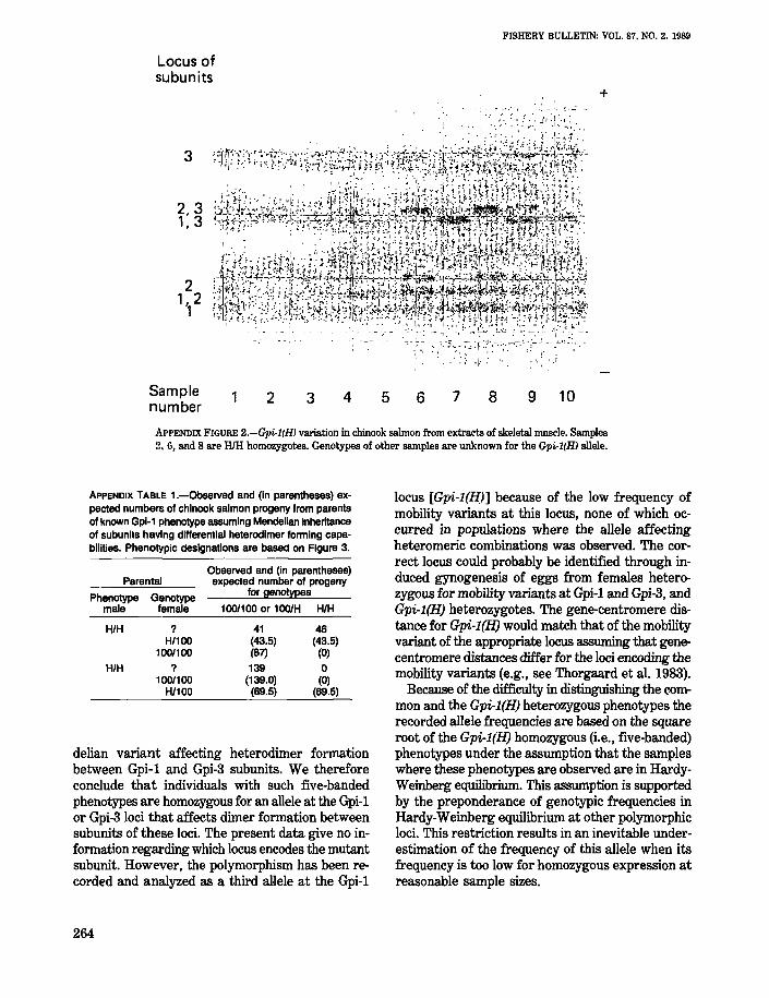
FISHERY BULLETIN: VOL. 87. NO.2. 1989

Locus ofsubunits

+

3

2,31,3

21,2

1

-'~. .

Samplenumber

2 3 4 5 6 7 8 9 10

ApPENDIX FIGURE 2.-Gpi-l(HJ variation in chinook salmon from extracts of skeletal muscle. Samples2. 6, and 8 are BIB homozygotes. Genotypes of other samples are unknown for the Gpi-l(HI allele.

H/H ? 41 46H/100 (43.5) (43.5)

1001100 (87) (0)

H/H ? 139 0100/100 (139.0) (0)

H/100 (69.5) (69.5)

locus [Gpi-l(.l:l)] because of the low frequency ofmobility variants at this locus, none of which oc­curred in populations where the allele affectingheteromeric combinations was observed. The cor­rect locus could probably be identified through in­duced gynogenesis of eggs from females hetero­zygous for mobility variants at Gpi-l and Gpi-3, andGpi-l(H) heterozygotes. The gene-centromere dis­tance for Gpi-l(H) would match that of the mobilityvariant of the appropriate locus assuming that gene­centromere distances differ for the loci encoding themobility variants (e.g., see Thorgaard et al. 1983).

Because of the difficulty in distinguishing the r.om­mon and the Gpi-l(H) heterozygous phenotypes therecorded allele frequencies are based on the squareroot of the Gpi-l(H) homozygous (i.e., five-banded)phenotypes under the assumption that the sampleswhere these phenotypes are observed are in Hardy­Weinberg equilibrium. This assumption is supportedby the preponderance of genotypic frequencies inHardy-Weinberg equilibrium at other polymorphicloci. This restriction results in an inevitable under­estimation of the frequency of this allele when itsfrequency is too low for homozygous expression atreasonable sample sizes.

100/100 or 100/H H/H

Parental

Phenotype Genotypemale female

ApPENDIX TABLE 1.-0bserved and (in parentheses) ex­pected numbers of chinook salmon progeny from parentsof known Gpi-1 phenotype assuming Mendelian inheritanceof subunits having differential heterodimer forming capa­bilities. Phenotypic designations are based on Figure 3.

Observed and (in parentheses)expected number of progeny

for genotrpes

delian variant affecting heterodimer formationbetween Gpi-l and Gpi-3 subunits. We thereforeconclude that individuals with such five-bandedphenotypes are homozygous for an allele at the Gpi-lor Gpi-3 loci that affects dimer formation betweensubunits of these loci. The present data give no in­formation regarding which locus encodes the mutantsubunit. However, the polymorphism has been re­corded and analyzed as a third allele at the Gpi-l

264