genetic algorithms

Genetic Algorithms

Chapter 3

A.E. Eiben and J.E. Smith, Introduction to Evolutionary ComputingGenetic Algorithms

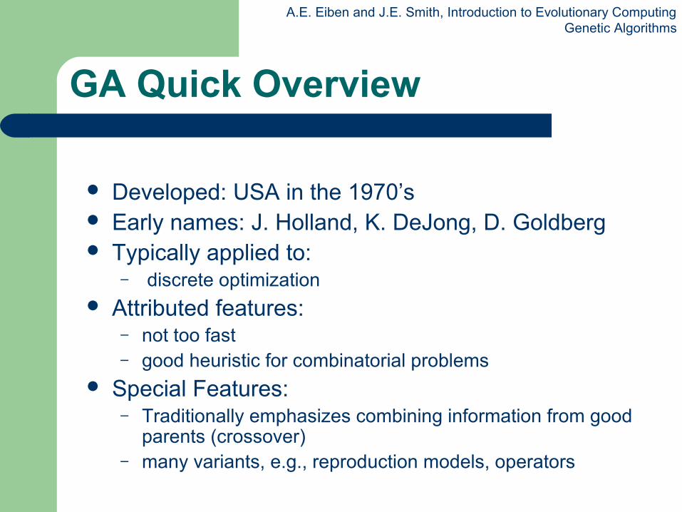
GA Quick Overview

Developed: USA in the 1970’s Early names: J. Holland, K. DeJong, D. Goldberg Typically applied to:

– discrete optimization Attributed features:

– not too fast– good heuristic for combinatorial problems

Special Features:– Traditionally emphasizes combining information from good

parents (crossover)– many variants, e.g., reproduction models, operators


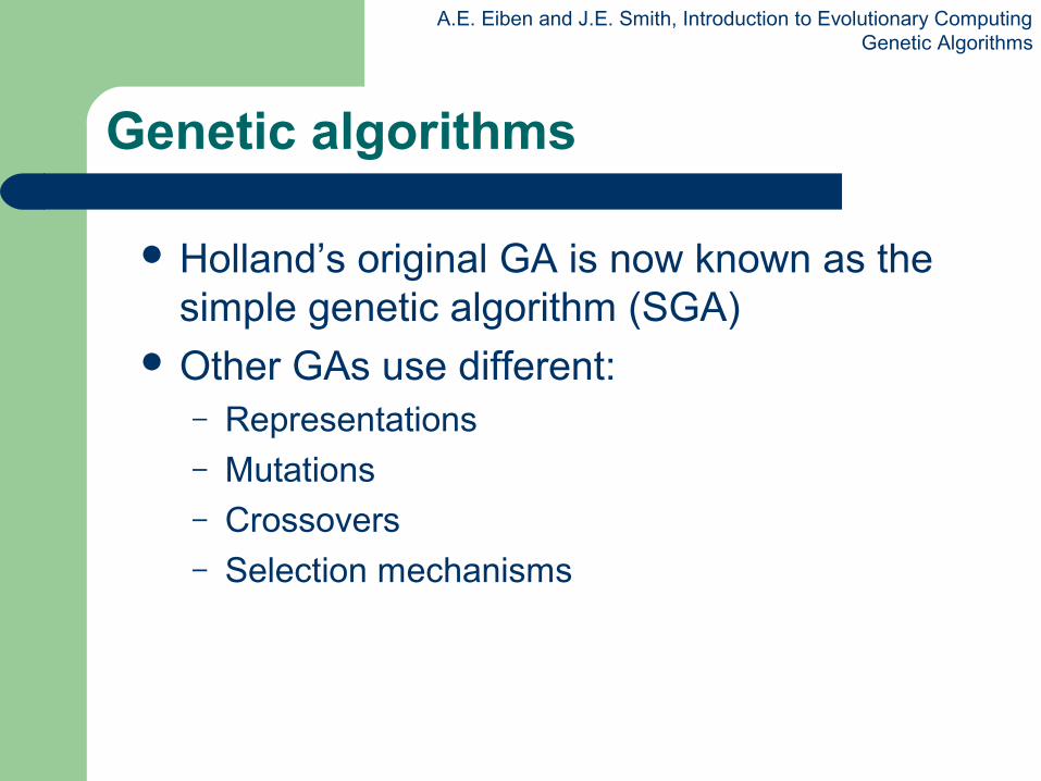
Genetic algorithms

Holland’s original GA is now known as the simple genetic algorithm (SGA)

Other GAs use different:– Representations– Mutations– Crossovers– Selection mechanisms


SGA technical summary tableau

Representation Binary strings

Recombination N-point or uniform

Mutation Bitwise bit-flipping with fixed probability

Parent selection Fitness-Proportionate

Survivor selection All children replace parents

Speciality Emphasis on crossover


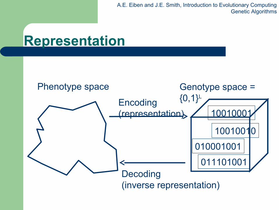
Genotype space = {0,1}L

Phenotype space

Encoding (representation)

Decoding(inverse representation)

011101001

010001001

10010010

10010001

Representation


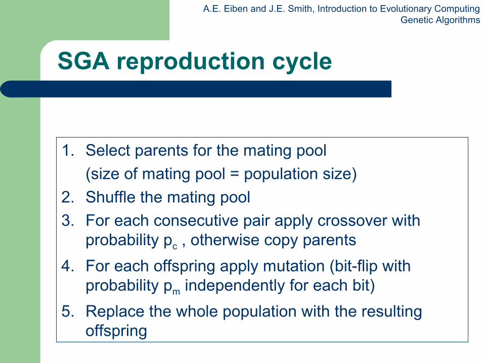
SGA reproduction cycle

1. Select parents for the mating pool

(size of mating pool = population size)

2. Shuffle the mating pool

3. For each consecutive pair apply crossover with probability pc , otherwise copy parents

4. For each offspring apply mutation (bit-flip with probability pm independently for each bit)

5. Replace the whole population with the resulting offspring


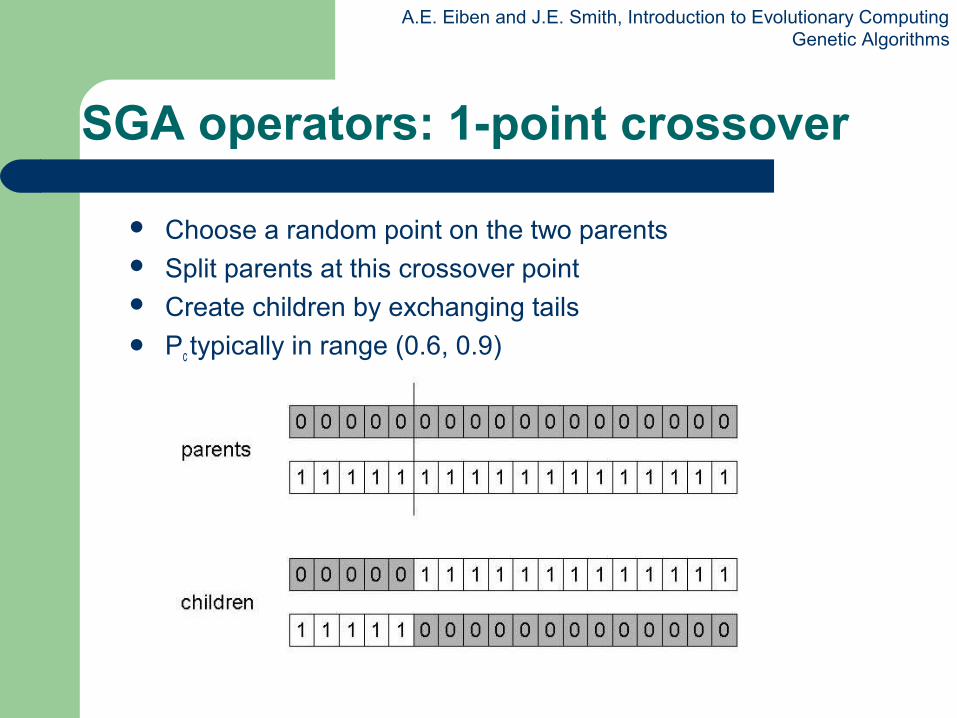
SGA operators: 1-point crossover

Choose a random point on the two parents Split parents at this crossover point Create children by exchanging tails Pc typically in range (0.6, 0.9)


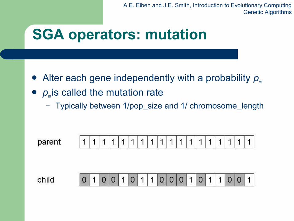
SGA operators: mutation

Alter each gene independently with a probability pm

pm is called the mutation rate– Typically between 1/pop_size and 1/ chromosome_length


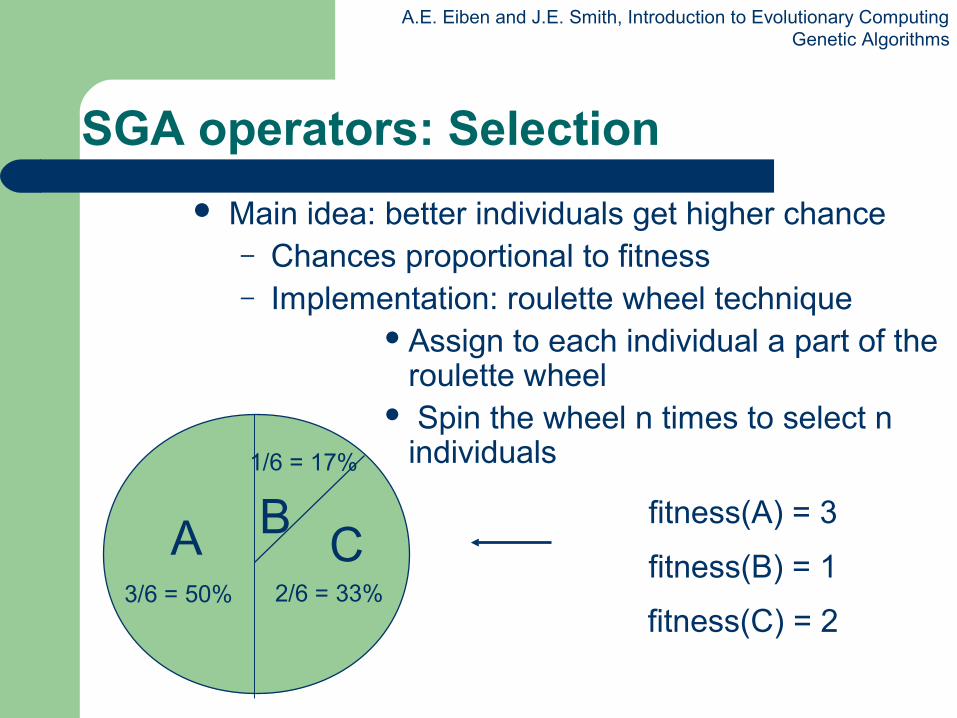
Main idea: better individuals get higher chance– Chances proportional to fitness– Implementation: roulette wheel technique

Assign to each individual a part of the roulette wheel

Spin the wheel n times to select n individuals

SGA operators: Selection

fitness(A) = 3

fitness(B) = 1

fitness(C) = 2

A C

1/6 = 17%

3/6 = 50%

B

2/6 = 33%


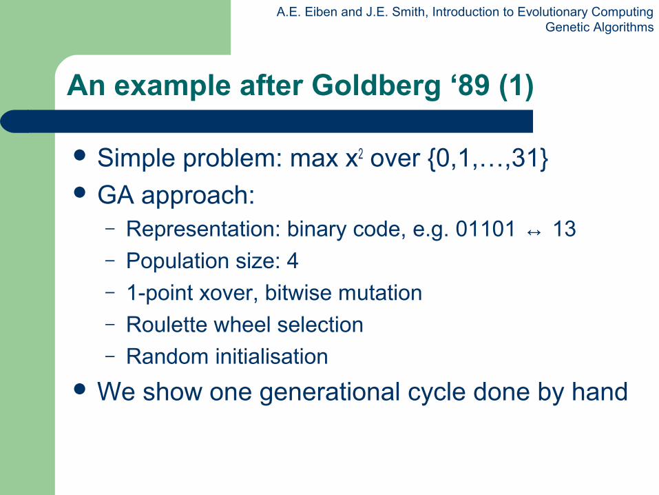
An example after Goldberg ‘89 (1)

Simple problem: max x2 over {0,1,…,31} GA approach:

– Representation: binary code, e.g. 01101 ↔ 13– Population size: 4– 1-point xover, bitwise mutation – Roulette wheel selection– Random initialisation

We show one generational cycle done by hand


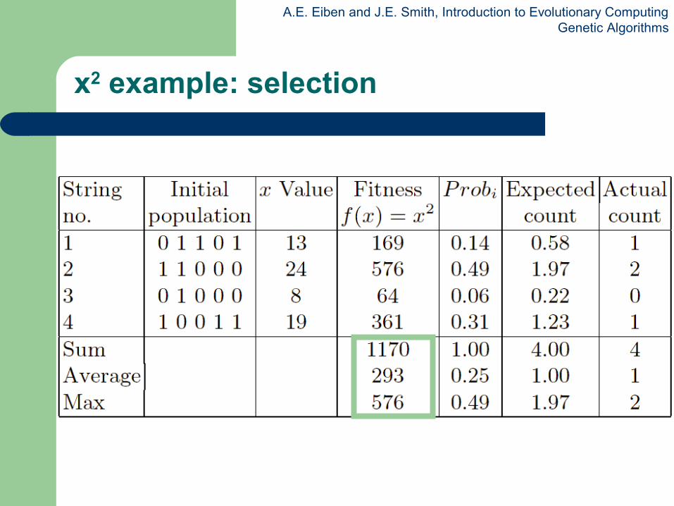
x2 example: selection


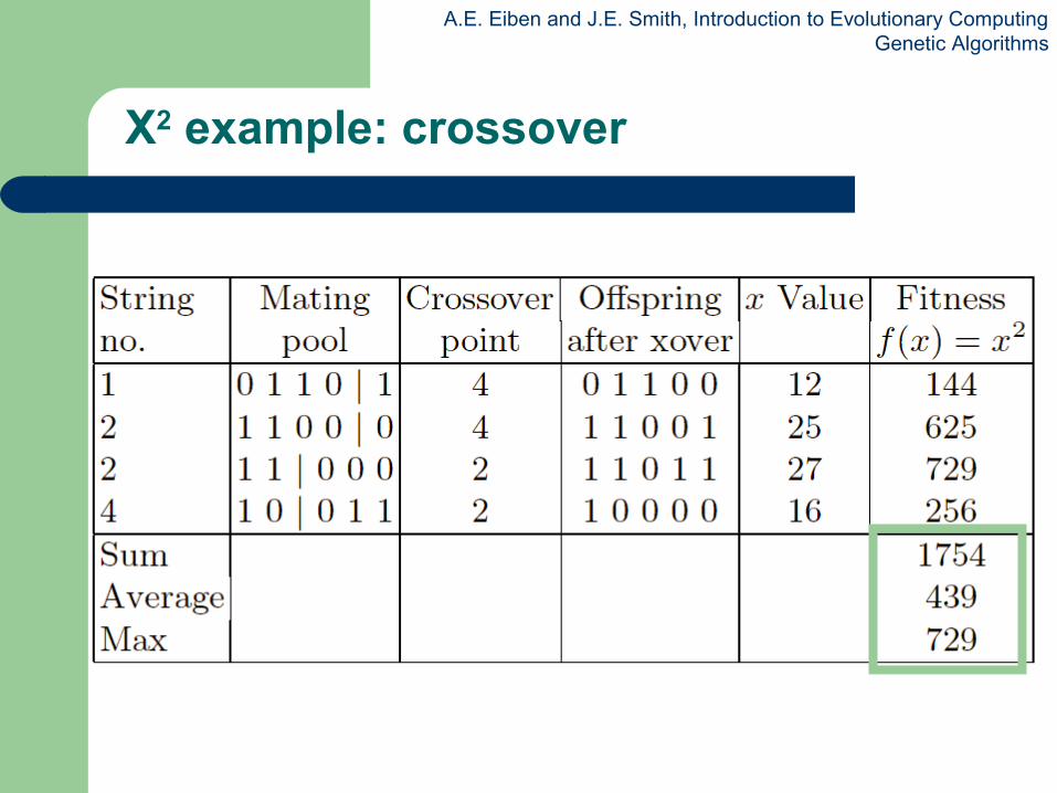
X2 example: crossover


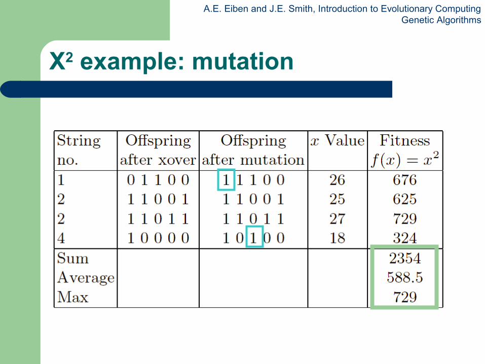
X2 example: mutation


The simple GA

Has been subject of many (early) studies– still often used as benchmark for novel GAs

Shows many shortcomings, e.g.– Representation is too restrictive– Mutation & crossovers only applicable for bit-string &

integer representations– Selection mechanism sensitive for converging

populations with close fitness values– Generational population model (step 5 in SGA repr.

cycle) can be improved with explicit survivor selection


Alternative Crossover Operators

Performance with 1 Point Crossover depends on the order that variables occur in the representation

– more likely to keep together genes that are near each other

– Can never keep together genes from opposite ends of string

– This is known as Positional Bias

– Can be exploited if we know about the structure of our problem, but this is not usually the case


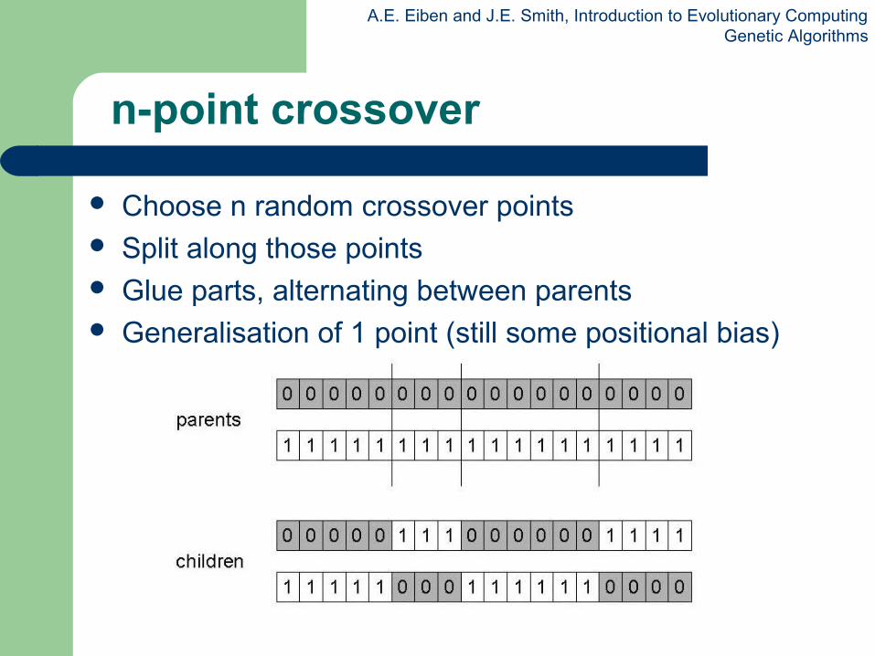
n-point crossover

Choose n random crossover points Split along those points Glue parts, alternating between parents Generalisation of 1 point (still some positional bias)


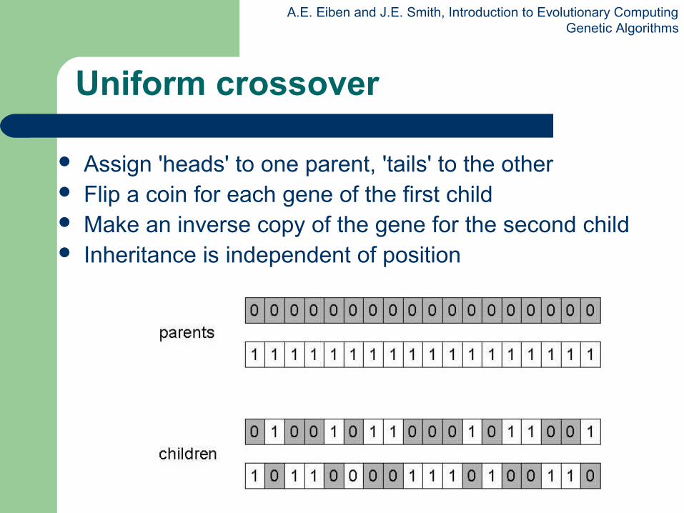
Uniform crossover

Assign 'heads' to one parent, 'tails' to the other Flip a coin for each gene of the first child Make an inverse copy of the gene for the second child Inheritance is independent of position


Crossover OR mutation?

Decade long debate: which one is better / necessary / main-background

Answer (at least, rather wide agreement):– it depends on the problem, but– in general, it is good to have both– both have another role– mutation-only-EA is possible, xover-only-EA would not work


Exploration: Discovering promising areas in the search

space, i.e. gaining information on the problem

Exploitation: Optimising within a promising area, i.e. using

information

There is co-operation AND competition between them

Crossover is explorative, it makes a big jump to an area

somewhere “in between” two (parent) areas

Mutation is exploitative, it creates random small

diversions, thereby staying near (in the area of ) the parent

Crossover OR mutation? (cont’d)


Only crossover can combine information from two

parents

Only mutation can introduce new information (alleles)

Crossover does not change the allele frequencies of

the population (thought experiment: 50% 0’s on first

bit in the population, ?% after performing n

crossovers)

To hit the optimum you often need a ‘lucky’ mutation

Crossover OR mutation? (cont’d)


Other representations

Gray coding of integers (still binary chromosomes)– Gray coding is a mapping that means that small changes in

the genotype cause small changes in the phenotype (unlike

binary coding). “Smoother” genotype-phenotype mapping

makes life easier for the GA

Nowadays it is generally accepted that it is better to

encode numerical variables directly as

Integers

Floating point variables


Integer representations

Some problems naturally have integer variables, e.g. image processing parameters

Others take categorical values from a fixed set e.g. {blue, green, yellow, pink}

N-point / uniform crossover operators work Extend bit-flipping mutation to make

– “creep” i.e. more likely to move to similar value– Random choice (esp. categorical variables)– For ordinal problems, it is hard to know correct range for

creep, so often use two mutation operators in tandem


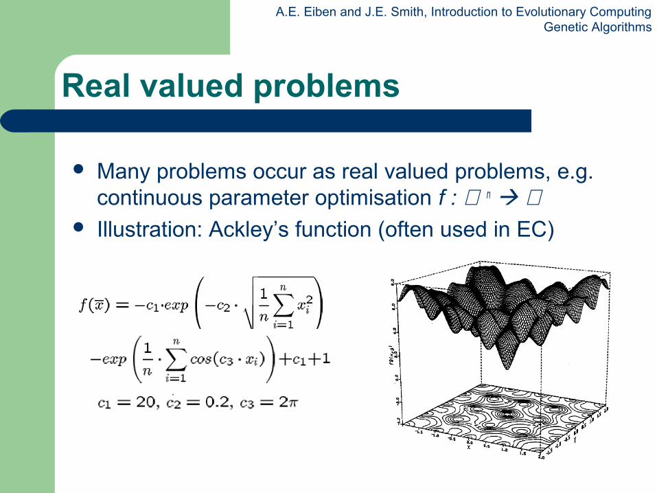
Real valued problems

Many problems occur as real valued problems, e.g. continuous parameter optimisation f : ℜ n ℜ

Illustration: Ackley’s function (often used in EC)


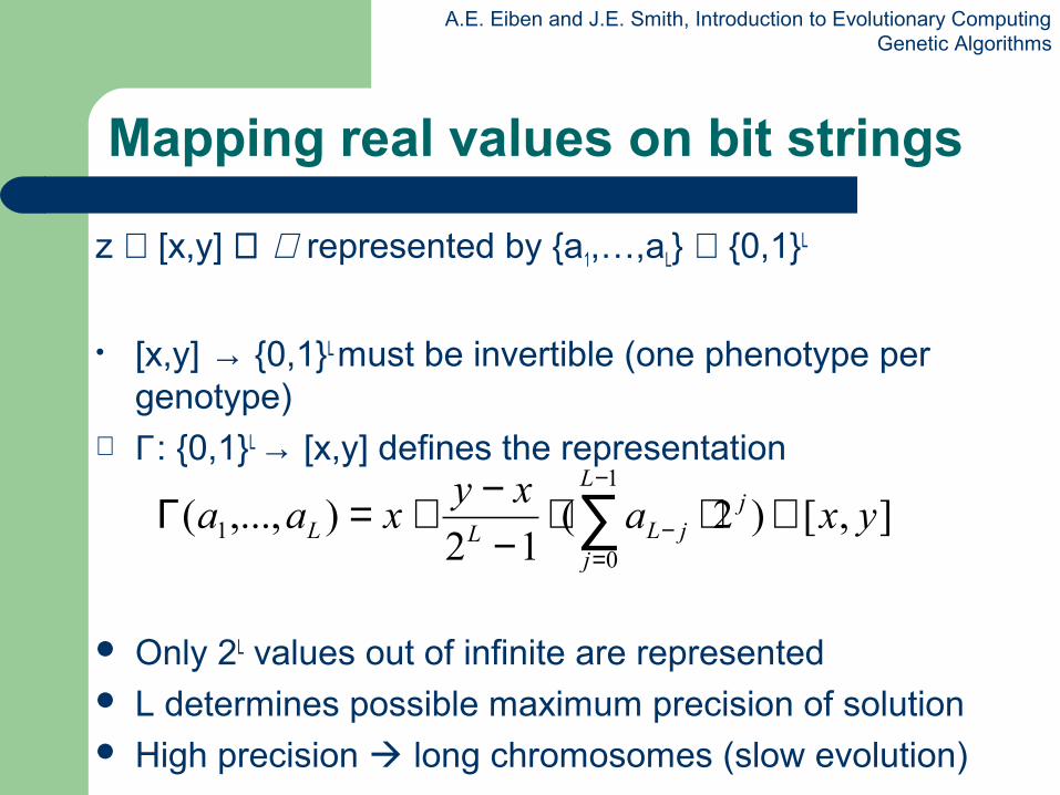
Mapping real values on bit strings

z ∈ [x,y] ⊆ ℜ represented by {a1,…,aL} ∈ {0,1}L

• [x,y] → {0,1}L must be invertible (one phenotype per genotype)

∀ Γ: {0,1}L → [x,y] defines the representation

Only 2L values out of infinite are represented L determines possible maximum precision of solution High precision long chromosomes (slow evolution)

],[)2(12

),...,(1

01 yxa

xyxaa j

L

jjLLL ∈⋅⋅

−−+=Γ ∑

−

=−


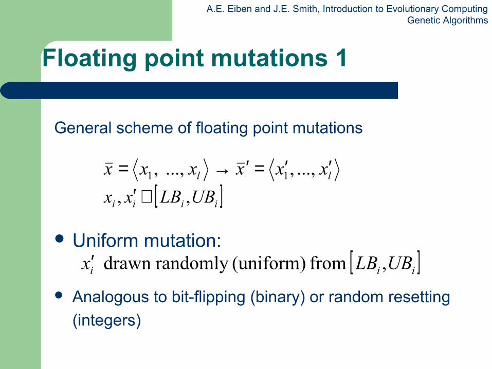
Floating point mutations 1

General scheme of floating point mutations

Uniform mutation:

Analogous to bit-flipping (binary) or random resetting

(integers)

ll xxxx xx ′′=′→= ..., , ...,, 11

[ ]iiii UBLBxx ,, ∈′

[ ]iii UBLBx , from (uniform)randomly drawn ′


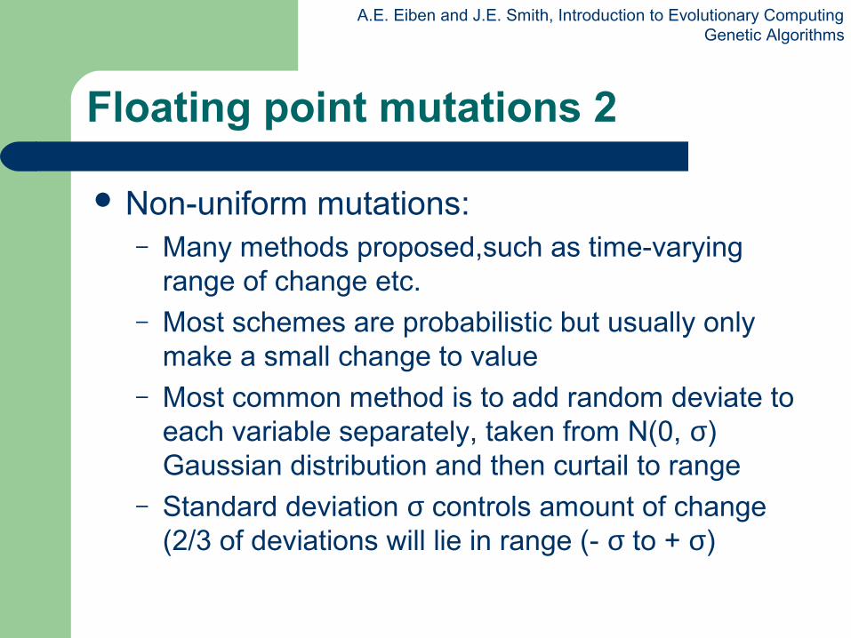
Floating point mutations 2

Non-uniform mutations:– Many methods proposed,such as time-varying

range of change etc.– Most schemes are probabilistic but usually only

make a small change to value– Most common method is to add random deviate to

each variable separately, taken from N(0, σ) Gaussian distribution and then curtail to range

– Standard deviation σ controls amount of change (2/3 of deviations will lie in range (- σ to + σ)


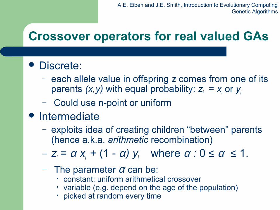
Crossover operators for real valued GAs

Discrete:– each allele value in offspring z comes from one of its

parents (x,y) with equal probability: zi = xi or yi

– Could use n-point or uniform Intermediate

– exploits idea of creating children “between” parents (hence a.k.a. arithmetic recombination)

– zi = α xi + (1 - α) yi where α : 0 ≤ α ≤ 1.– The parameter α can be:

• constant: uniform arithmetical crossover• variable (e.g. depend on the age of the population) • picked at random every time


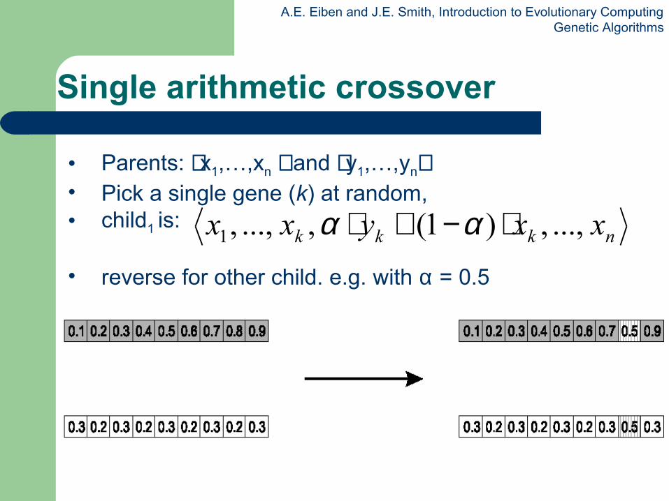
Single arithmetic crossover

• Parents: ⟨x1,…,xn ⟩ and ⟨y1,…,yn⟩• Pick a single gene (k) at random, • child1 is:

• reverse for other child. e.g. with α = 0.5

nkkk xxyxx ..., ,)1( , ..., ,1 ⋅−+⋅ αα


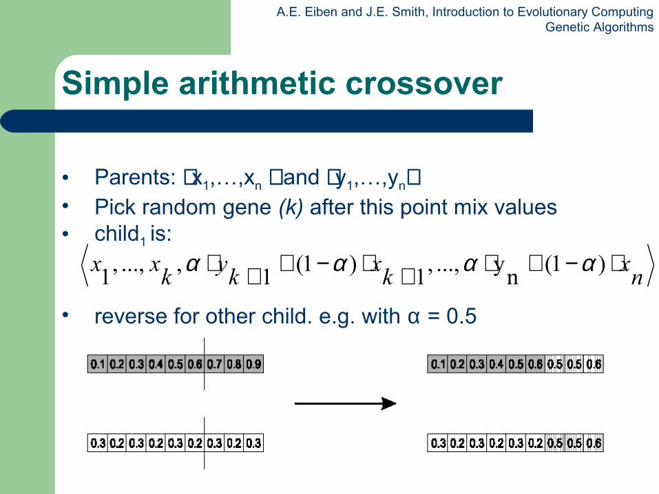
Simple arithmetic crossover

• Parents: ⟨x1,…,xn ⟩ and ⟨y1,…,yn⟩• Pick random gene (k) after this point mix values• child1 is:


nx

kx

ky

kxx ⋅−+⋅+⋅−++⋅ )1(

ny ..., ,

1)1(

1 , ..., ,

1αααα


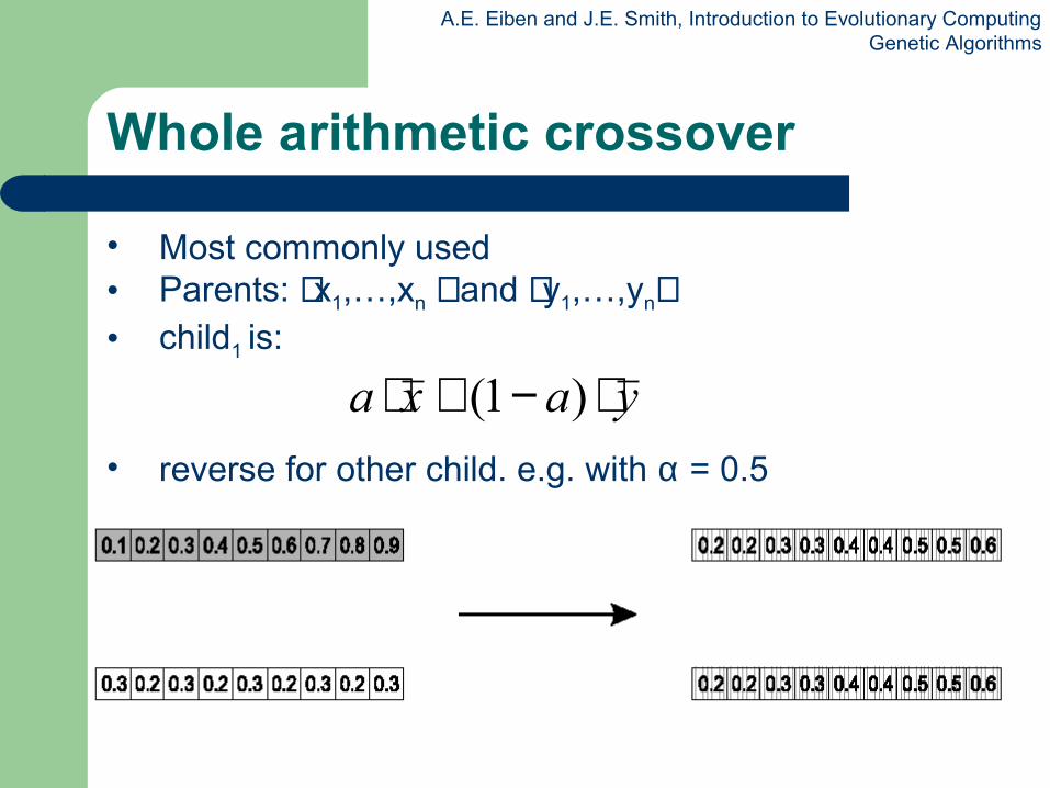
• Most commonly used• Parents: ⟨x1,…,xn ⟩ and ⟨y1,…,yn⟩• child1 is:


Whole arithmetic crossover

yaxa ⋅−+⋅ )1(


Permutation Representations

Ordering/sequencing problems form a special type Task is (or can be solved by) arranging some objects in

a certain order – Example: sort algorithm: important thing is which elements

occur before others (order)– Example: Travelling Salesman Problem (TSP) : important thing

is which elements occur next to each other (adjacency)

These problems are generally expressed as a permutation:– if there are n variables then the representation is as a list of n

integers, each of which occurs exactly once


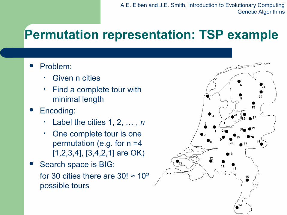
Permutation representation: TSP example

Problem:• Given n cities• Find a complete tour with

minimal length Encoding:

• Label the cities 1, 2, … , n• One complete tour is one

permutation (e.g. for n =4 [1,2,3,4], [3,4,2,1] are OK)

Search space is BIG:

for 30 cities there are 30! ≈ 1032 possible tours


Mutation operators for permutations

Normal mutation operators lead to inadmissible solutions– e.g. bit-wise mutation : let gene i have value j– changing to some other value k would mean that k

occurred twice and j no longer occurred

Therefore must change at least two values Mutation parameter now reflects the probability

that some operator is applied once to the whole string, rather than individually in each position


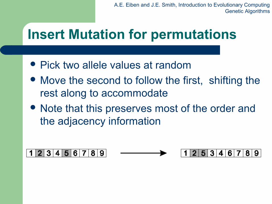
Insert Mutation for permutations

Pick two allele values at random Move the second to follow the first, shifting the

rest along to accommodate Note that this preserves most of the order and

the adjacency information


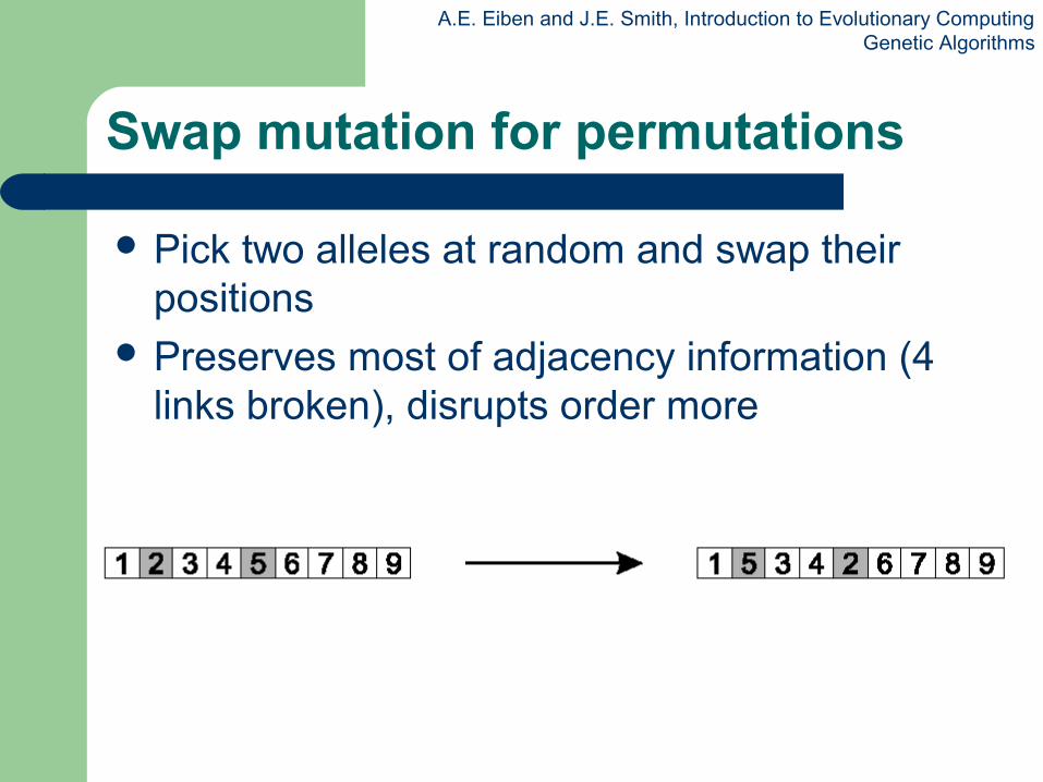
Swap mutation for permutations

Pick two alleles at random and swap their positions

Preserves most of adjacency information (4 links broken), disrupts order more


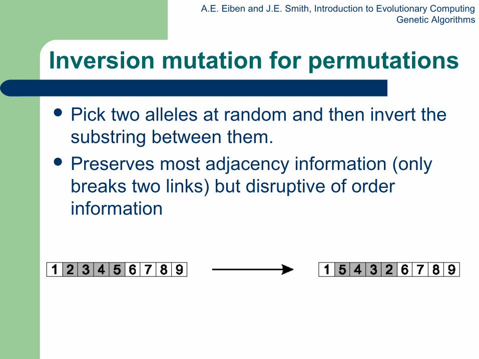
Inversion mutation for permutations

Pick two alleles at random and then invert the substring between them.

Preserves most adjacency information (only breaks two links) but disruptive of order information


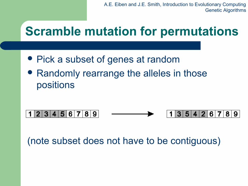
Scramble mutation for permutations

Pick a subset of genes at random Randomly rearrange the alleles in those

positions

(note subset does not have to be contiguous)


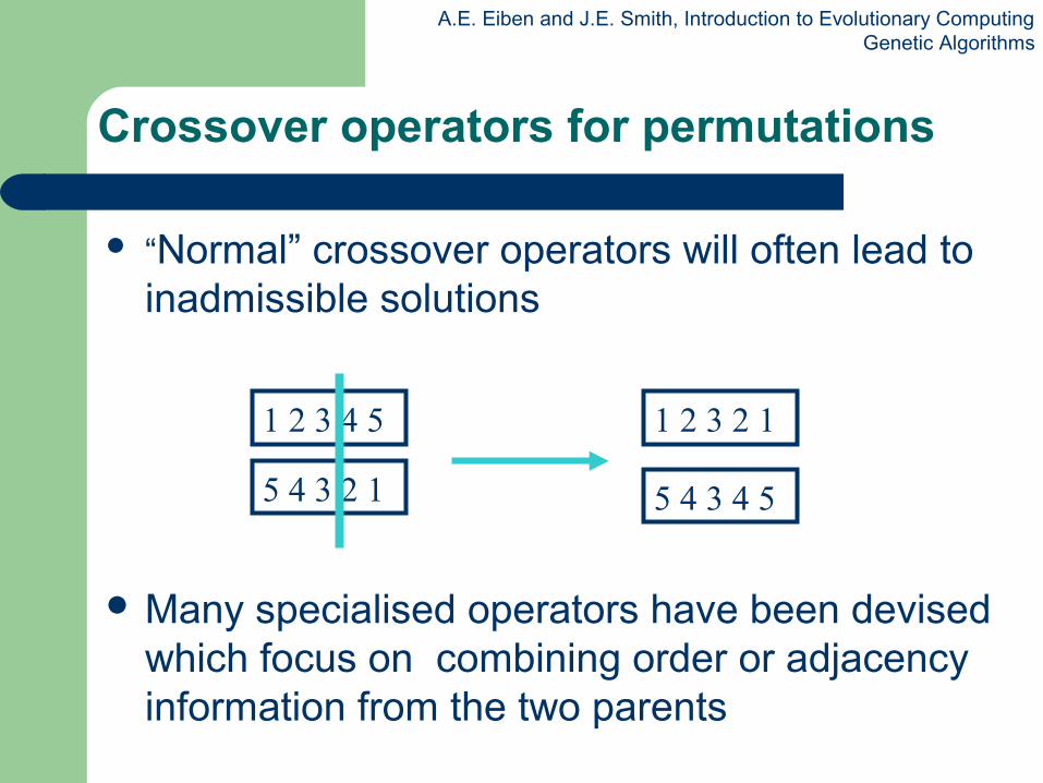
“Normal” crossover operators will often lead to inadmissible solutions

Many specialised operators have been devised which focus on combining order or adjacency information from the two parents

Crossover operators for permutations

1 2 3 4 5

5 4 3 2 1

1 2 3 2 1

5 4 3 4 5


Order 1 crossover

Idea is to preserve relative order that elements occur Informal procedure:

1. Choose an arbitrary part from the first parent

2. Copy this part to the first child

3. Copy the numbers that are not in the first part, to the first child:

starting right from cut point of the copied part, using the order of the second parent and wrapping around at the end

4. Analogous for the second child, with parent roles reversed


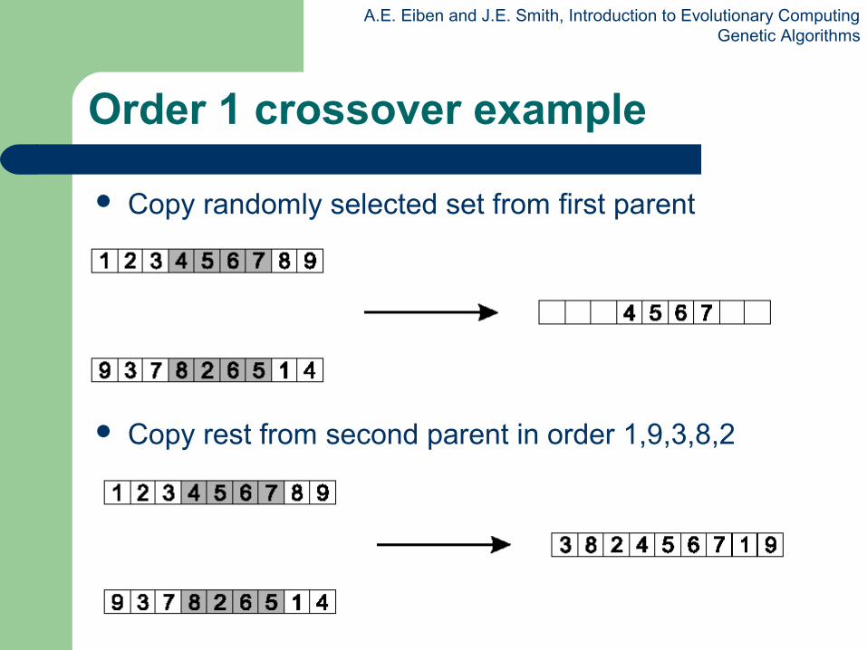
Order 1 crossover example

Copy randomly selected set from first parent

Copy rest from second parent in order 1,9,3,8,2


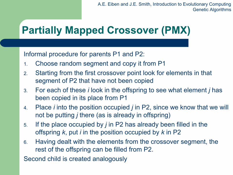
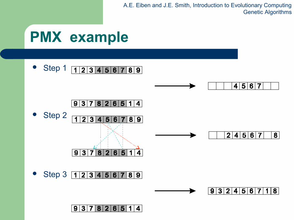
Informal procedure for parents P1 and P2:

1. Choose random segment and copy it from P1

2. Starting from the first crossover point look for elements in that segment of P2 that have not been copied

3. For each of these i look in the offspring to see what element j has been copied in its place from P1

4. Place i into the position occupied j in P2, since we know that we will not be putting j there (as is already in offspring)

5. If the place occupied by j in P2 has already been filled in the offspring k, put i in the position occupied by k in P2

6. Having dealt with the elements from the crossover segment, the rest of the offspring can be filled from P2.

Second child is created analogously

Partially Mapped Crossover (PMX)


PMX example

Step 1

Step 2

Step 3


Cycle crossover

Basic idea:

Each allele comes from one parent together with its position.

Informal procedure:1. Make a cycle of alleles from P1 in the following way.

(a) Start with the first allele of P1.

(b) Look at the allele at the same position in P2.

(c) Go to the position with the same allele in P1.

(d) Add this allele to the cycle.

(e) Repeat step b through d until you arrive at the first allele of P1.

2. Put the alleles of the cycle in the first child on the positions they have in the first parent.

3. Take next cycle from second parent


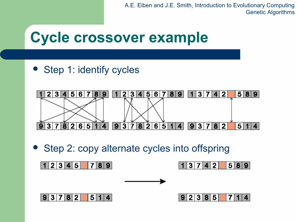
Cycle crossover example

Step 1: identify cycles

Step 2: copy alternate cycles into offspring


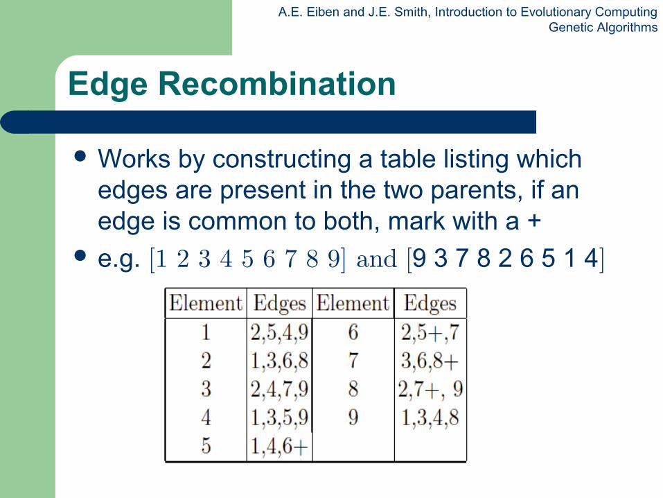
Edge Recombination

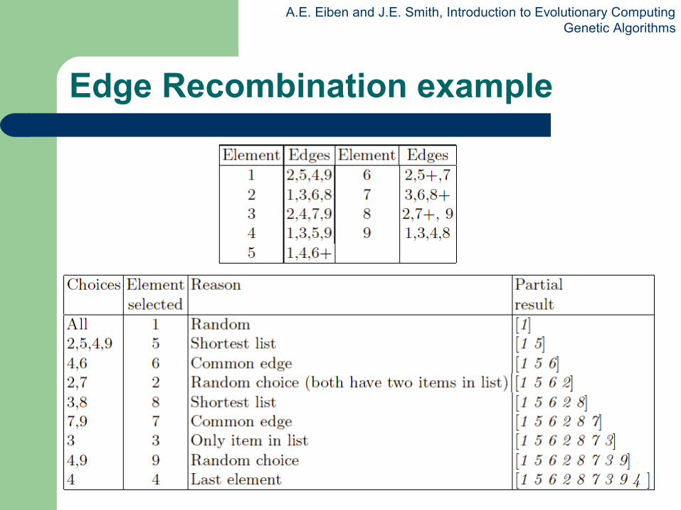
Works by constructing a table listing which edges are present in the two parents, if an edge is common to both, mark with a +

e.g. [1 2 3 4 5 6 7 8 9] and [9 3 7 8 2 6 5 1 4]


Edge Recombination 2

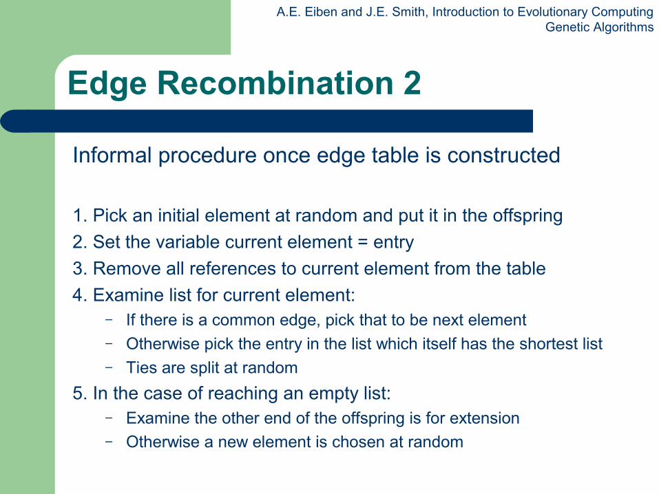
Informal procedure once edge table is constructed

1. Pick an initial element at random and put it in the offspring

2. Set the variable current element = entry

3. Remove all references to current element from the table

4. Examine list for current element:– If there is a common edge, pick that to be next element– Otherwise pick the entry in the list which itself has the shortest list– Ties are split at random

5. In the case of reaching an empty list:– Examine the other end of the offspring is for extension– Otherwise a new element is chosen at random


Edge Recombination example


Multiparent recombination

Recall that we are not constricted by the practicalities of nature

Noting that mutation uses 1 parent, and “traditional” crossover 2, the extension to a>2 is natural to examine

Been around since 1960s, still rare but studies indicate useful

Three main types:– Based on allele frequencies, e.g., p-sexual voting generalising

uniform crossover– Based on segmentation and recombination of the parents, e.g.,

diagonal crossover generalising n-point crossover– Based on numerical operations on real-valued alleles, e.g.,

center of mass crossover, generalising arithmetic recombination operators


Population Models

SGA uses a Generational model:– each individual survives for exactly one generation– the entire set of parents is replaced by the offspring

At the other end of the scale are Steady-State models:– one offspring is generated per generation,– one member of population replaced,

Generation Gap – the proportion of the population replaced– 1.0 for GGA, 1/pop_size for SSGA


Fitness Based Competition

Selection can occur in two places:– Selection from current generation to take part in

mating (parent selection) – Selection from parents + offspring to go into next

generation (survivor selection)

Selection operators work on whole individual– i.e. they are representation-independent

Distinction between selection– operators: define selection probabilities – algorithms: define how probabilities are implemented


Implementation example: SGA

Expected number of copies of an individual i

E( ni ) = µ • f(i)/ ⟨ f⟩

(µ = pop.size, f(i) = fitness of i, ⟨ f⟩ avg. fitness in pop.)

Roulette wheel algorithm:– Given a probability distribution, spin a 1-armed

wheel n times to make n selections– No guarantees on actual value of ni

Baker’s SUS algorithm:– n evenly spaced arms on wheel and spin once

– Guarantees floor(E( ni ) ) ≤ ni ≤ ceil(E( ni ) )


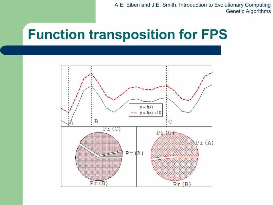
Problems include– One highly fit member can rapidly take over if rest of

population is much less fit: Premature Convergence– At end of runs when fitnesses are similar, lose

selection pressure – Highly susceptible to function transposition

Scaling can fix last two problems– Windowing: f’(i) = f(i) - β t

where β is worst fitness in this (last n) generations

– Sigma Scaling: f’(i) = max( f(i) – (⟨ f ⟩ - c • σf ), 0.0) where c is a constant, usually 2.0

Fitness-Proportionate Selection


Function transposition for FPS


Rank – Based Selection

Attempt to remove problems of FPS by basing selection probabilities on relative rather than absolute fitness

Rank population according to fitness and then base selection probabilities on rank where fittest has rank µ and worst rank 1

This imposes a sorting overhead on the algorithm, but this is usually negligible compared to the fitness evaluation time


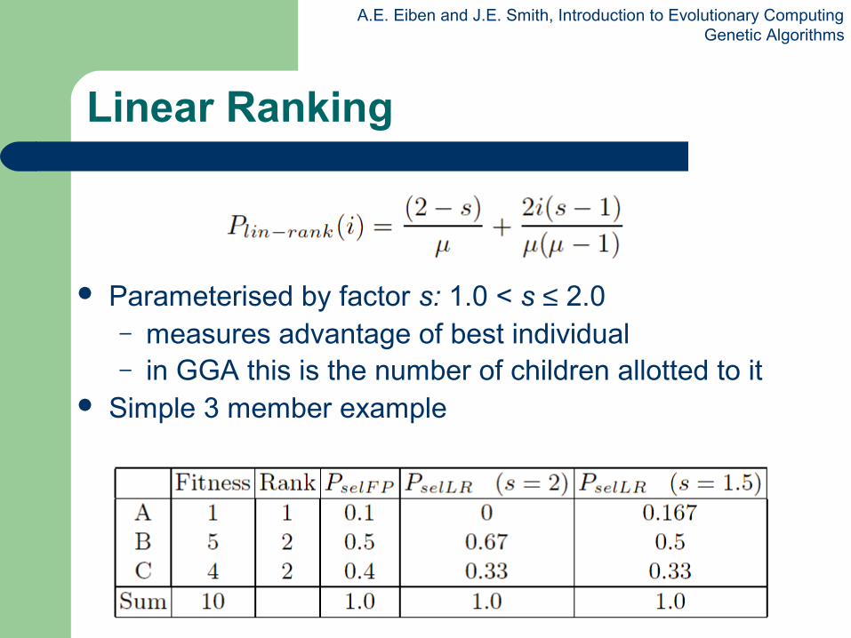
Linear Ranking

Parameterised by factor s: 1.0 < s ≤ 2.0– measures advantage of best individual– in GGA this is the number of children allotted to it

Simple 3 member example


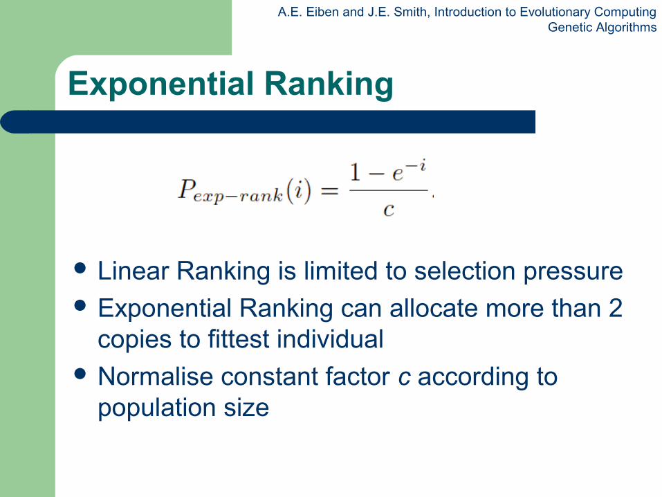
Exponential Ranking

Linear Ranking is limited to selection pressure Exponential Ranking can allocate more than 2

copies to fittest individual Normalise constant factor c according to

population size


Tournament Selection

All methods above rely on global population statistics– Could be a bottleneck esp. on parallel machines– Relies on presence of external fitness function

which might not exist: e.g. evolving game players

Informal Procedure:– Pick k members at random then select the best of

these– Repeat to select more individuals


Tournament Selection 2

Probability of selecting i will depend on:– Rank of i– Size of sample k

higher k increases selection pressure– Whether contestants are picked with replacement

Picking without replacement increases selection pressure

– Whether fittest contestant always wins (deterministic) or this happens with probability p

For k = 2, time for fittest individual to take over

population is the same as linear ranking with s = 2 • p


Survivor Selection

Most of methods above used for parent selection

Survivor selection can be divided into two approaches:– Age-Based Selection

e.g. SGA In SSGA can implement as “delete-random” (not

recommended) or as first-in-first-out (a.k.a. delete-oldest)

– Fitness-Based Selection Using one of the methods above or


Two Special Cases

Elitism– Widely used in both population models (GGA,

SSGA)– Always keep at least one copy of the fittest solution

so far

GENITOR: a.k.a. “delete-worst”– From Whitley’s original Steady-State algorithm (he

also used linear ranking for parent selection)– Rapid takeover : use with large populations or “no

duplicates” policy


Example application of order based GAs: JSSP

Precedence constrained job shop scheduling problem J is a set of jobs. O is a set of operations M is a set of machines Able ⊆ O × M defines which machines can perform which

operations Pre ⊆ O × O defines which operation should precede which Dur : ⊆ O × M → IR defines the duration of o ∈ O on m ∈ M

The goal is now to find a schedule that is: Complete: all jobs are scheduled Correct: all conditions defined by Able and Pre are satisfied Optimal: the total duration of the schedule is minimal


Precedence constrained job shop scheduling GA

Representation: individuals are permutations of operations Permutations are decoded to schedules by a decoding procedure

– take the first (next) operation from the individual– look up its machine (here we assume there is only one)– assign the earliest possible starting time on this machine, subject to

machine occupation precedence relations holding for this operation in the schedule created so far

fitness of a permutation is the duration of the corresponding schedule (to be minimized)

use any suitable mutation and crossover use roulette wheel parent selection on inverse fitness Generational GA model for survivor selection use random initialisation


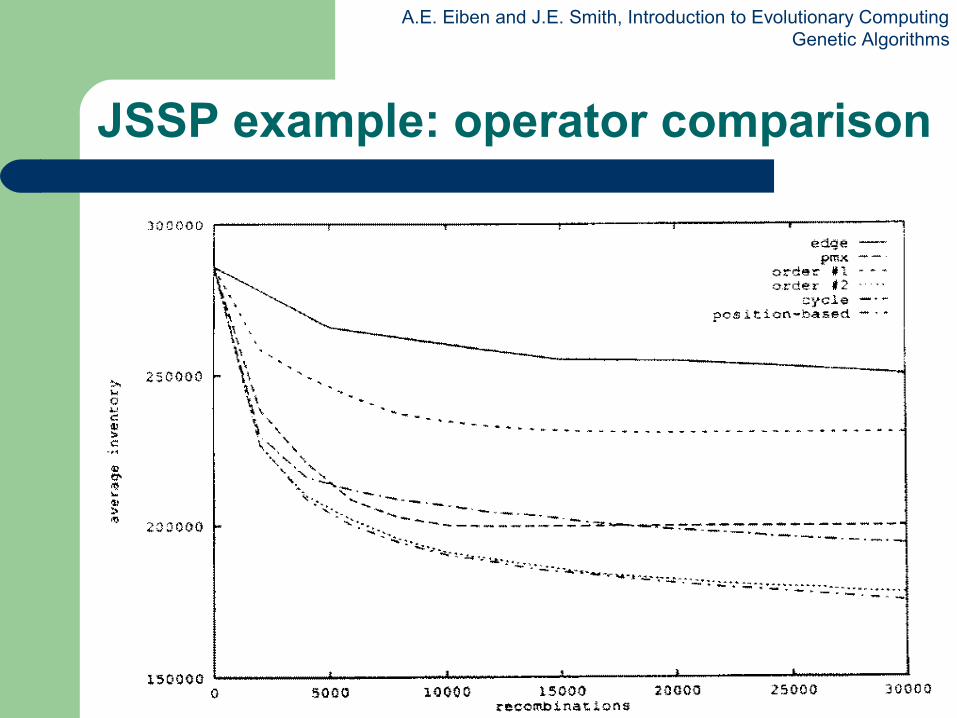
JSSP example: operator comparison

genetic algorithms

Education

probability pm pm

roulette wheel techniqueassign

wheel n times

mating poolfor

parentssplit parents

simple problem

population sizeshuffle

mutation ratetypically