Mathematical and Computer Modelling 57 (2013) 2596–2604

Contents lists available at SciVerse ScienceDirect

Mathematical and Computer Modelling

journal homepage: www.elsevier.com/locate/mcm

Generation of pseudorandom binary sequences by means of linearfeedback shift registers (LFSRs) with dynamic feedbackA. Peinado a,∗, A. Fúster-Sabater ba Departamento de Ingeniería de, Comunicaciones, Universidad de Málaga, Campus de Teatinos - 29071 Malaga, Spainb Institute of Applied Physics, C.S.I.C., Serrano 144, 28006 Madrid, Spain

a r t i c l e i n f o

Article history:Received 27 December 2010Received in revised form 3 June 2011Accepted 18 July 2011

Keywords:DLFSRPseudorandom sequence generatorInterleaved sequenceCryptography

a b s t r a c t

In 2002, Mita et al. [1] proposed a pseudorandom bit generator based on a dynamiclinear feedback shift register (DLFSR) for cryptographic application. The particular topologythere proposed is now analyzed, allowing us to extend the results to more generalcases. Maximum period and linear span values are obtained for the generated sequences,while several estimations for autocorrelation and cross-correlation of such sequences arealso presented. Furthermore, the sequences produced by DLFSRs can be considered asinterleaved sequences. This fact allows us to apply the general interleaved sequencemodelproposed byGong and consequently simplify their study. Finally, several remarks are statedregarding DLFSR utilization for cryptographic or code division multiple access (CDMA)applications.

© 2011 Elsevier Ltd. All rights reserved.

1. Introduction

In [1], Mita et al. proposed a new pseudorandombinary sequence generator for cryptographic application based on linearfeedback shift registers (LFSRs) that they called ‘‘topology with dynamic linear feedback shift register’’ (DLFSR). In fact, sucha topology consists in changing dynamically the feedback polynomial of the LFSR that generates the output sequence. For ageneral overview of LFSRs, the interested reader is referred to [2].

In [1], that DLFSR topology is introduced in a generic way, providing only a few pieces of experimental data from a par-ticular implementation. In addition, Mita et al. claimed that the proposed generator satisfied the same pseudorandomnessrequirements as those of LFSRs in addition to greatly improving the violability performance. Nevertheless, they did not pro-vide the reader with theoretical/practical considerations concerning cryptographic parameters of the generated sequences,e.g. period or linear span [3].

In thiswork, upper bounds on the linear span and the period of a genericDLFSR are computed and applied to the particularconfiguration introduced in [1]. In this way, it is proved that, in spite of the authors’ claim, the proposed configuration isnot the best possible. In fact, there are other configurations that are able to generate sequences with greater period and/orlinear span.

As far as cryptographic application is concerned, it must be said that the DLFSR generator introduced in [1] is not at allthe best choice. On the one hand, it is difficult to design this kind of generator with arbitrary parameters while keepinga minimum level of quality in the generated sequences. On the other hand, the correlation among different sequencesproduced by the same generator does not recommend its use.

In brief, this work evaluates the possible utilization of the DLFSR generator for cryptographic and/or code divisionmultiple access (CDMA) applications.

∗ Corresponding author. Tel.: +34 952131305; fax: +34 952132027.E-mail addresses: apeinado@ic.uma.es (A. Peinado), amparo@iec.csic.es (A. Fúster-Sabater).

0895-7177/$ – see front matter© 2011 Elsevier Ltd. All rights reserved.doi:10.1016/j.mcm.2011.07.023

A. Peinado, A. Fúster-Sabater / Mathematical and Computer Modelling 57 (2013) 2596–2604 2597

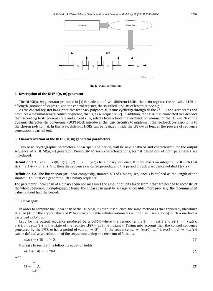
Fig. 1. DLFSR architecture.

2. Description of the DLFSR(n,m) generator

The DLFSR(n,m) generator proposed in [1] is made out of two different LFSRs: the main register, the so-called LFSR-n,of length (number of stages) n, and the control register, the so-called LFSR-m, of lengthm. See Fig. 1.

As the control register has a primitive feedback polynomial, it runs cyclically through all the 2m− 1 non-zero states and

produces a maximal-length control sequence, that is, a PN-sequence [2]. In addition, the LFSR-m is connected to a decoderthat, according to its present state and a fixed rule, selects from a table the feedback polynomial of the LFSR-n. Next, thedynamic characteristic polynomial (DCP) block introduces the logic circuitry to implement the feedback corresponding tothe chosen polynomial. In this way, different LFSRs can be realized inside the LFSR-n as long as the process of sequencegeneration is carried out.

3. Characterization of the DLFSR(n,m) generator parameters

Two basic cryptographic parameters, linear span and period, will be next analyzed and characterized for the outputsequence of a DLFSR(n,m) generator. Previously to such characterizations, formal definitions of both parameters areintroduced.

Definition 3.1. Let s = (s(0), s(1), s(2), . . .) = (s(t)) be a binary sequence. If there exists an integer r > 0 such thats(t) = s(t + r) for all t ≥ 0, then the sequence s is called periodic, and the period of such a sequence notated T (s) is r .

Definition 3.2. The linear span (or linear complexity, notated LC) of a binary sequence s is defined as the length of theshortest LFSR that can generate such a binary sequence.

The parameter linear span of a binary sequence measures the amount of bits taken from s that are needed to reconstructthe whole sequence. In cryptographic terms, the linear spanmust be as large as possible; more precisely, the recommendedvalue is about half the period.

3.1. Linear span

In order to compute the linear span of the DLFSR(n,m) output sequence, the same method as that applied by Blackburnet al. in [4] for the cryptanalysis of PCAs (programmable cellular automata) will be used; see also [5]. Such a method isdescribed as follows.

Let s be the output sequence produced by a DLFSR where the generic term s(t) = v0(t) and v(t) = (v0(t),v1(t), . . . , vn−1(t)) is the state of the register LFSR-n at time instant t . Taking into account that the control sequencegenerated by the LFSR-m has a period of value l = 2m

− 1, the sequence ω0 = (ω0(0), ω0(1), ω0(2), . . .) = (ω0(t))can be defined as a decimation of the sequence s taking one term out of l; that is,

ω0(t) = s(tl) t ≥ 0. (1)

It is easy to see that the following equation holds:

v((t + 1)l) = v(tl)M, (2)

with

M =

l−1i=0

Ai, (3)

2598 A. Peinado, A. Fúster-Sabater / Mathematical and Computer Modelling 57 (2013) 2596–2604

Ai being an n × nmatrix whose characteristic polynomial is the feedback polynomial of the register LFSR-n at time ti. Thus,it can be written that

ω0(t) = πM tv(0), (4)

where π is a linear map of an n-dimension vector space over GF(2) that transforms (v0(t), v1(t), . . . , vn−1(t)) into v0(t).If the characteristic polynomial of the matrix M is c(x) =

ni=0 cix

i, then the Cayley–Hamilton theorem [6] states thatevery square matrixM satisfies its characteristic equation. That is,

c(M) = cnMn+ cn−1Mn−1

+ · · · + c1M + c0I = 0. (5)

Thus,n

i=0

ciω0(t + i) =

ni=0

ci πM t+iv(0) = πM tc(M)v(0) = 0. (6)

Since ω0(t + n) can be written as a linear combination of the previous n terms, the linear span of the sequence ω0 is atmost n. The same reasoning can be applied to any of the other decimated sequences ωj whose generic terms are defined as

ωj(t) = s(tl + j) 0 ≤ j ≤ (l − 1). (7)

In this way, the sequence s can be obtained by interleaving l different sequences ωj, where each one of them has a linearspan LC ≤ n. Thus, the linear span of s is upper bounded as follows:

LC(s) ≤ n · l. (8)

That is to say, the sequence s can be reconstructed from the knowledge of at most 2nl bits [7].

Remark 1. For the particular case DLFSR(16, 5) proposed in [1], the computation of M in Eq. (3) does not require themultiplication of l = 31 matrices, as only four feedback polynomials are defined. Consequently, there will be only fourdifferent matrices (A1, A2, A3, A4) (see Section 4), and the matrixM corresponding to the sequence ω0 will be

M = A91A

52A3A16

4 . (9)

3.2. Maximum period

Keeping in mind that the sequence s can be written by interleaving l sequences ωj, it is clear that the period T (s) of sucha sequence is determined by the periods T (ωj) of the sequences ωj in the following way:

T (s) = lcm[T (ωj)] · l 0 ≤ j ≤ (l − 1), (10)

where lcm stands for least commonmultiple, l is the number of interleaved sequences. If the n×nmatrixMj is the generatingmatrix of the sequence ωj for 0 ≤ j ≤ (l − 1), then the period T (ωj) will always be less than or equal to 2n

− 1, and will bedetermined by the characteristic polynomial cj(x) ofMj [8].

Definition 3.3 ([9]). Let p be a non-zero polynomial with binary coefficients. If p(0) = 0, then the least positive integer efor which p(x) divides xe + 1 is called the period of p, and is denoted by per(p) = per(p(x)). If p(0) = 0, then p(x) = xhq(x),where h ∈ N and per(p) is defined to be per(q).

From the previous definition, Eq. (10) can be rewritten as

T (s) = lcm[per(cj(x))] · l 0 ≤ j ≤ (l − 1). (11)

On the other hand, if L represents the left-shift cyclic operator on the matrix product, that is,

L(A1, A2, A3, A4) = A2 A3 A4 A1, (12)

then the following lemma will allow us to simplify Eq. (11).

Lemma 3.4. Let A and B be two n × n matrices and cA(x), cB(x) their corresponding characteristic polynomials. Then, thecharacteristic polynomial cAB(x) of the matrix product AB equals the characteristic polynomial cBA(x) of the matrix product BA.

Proof. The characteristic polynomial of matrix A is cA(x) = det(xI − A). Then the polynomial of the matrix AB can becomputed as

cAB(x) = det(xI − AB)= det(A−1(xI − AB)A)

= det(xI − BA) = cBA(x). � (13)

A. Peinado, A. Fúster-Sabater / Mathematical and Computer Modelling 57 (2013) 2596–2604 2599

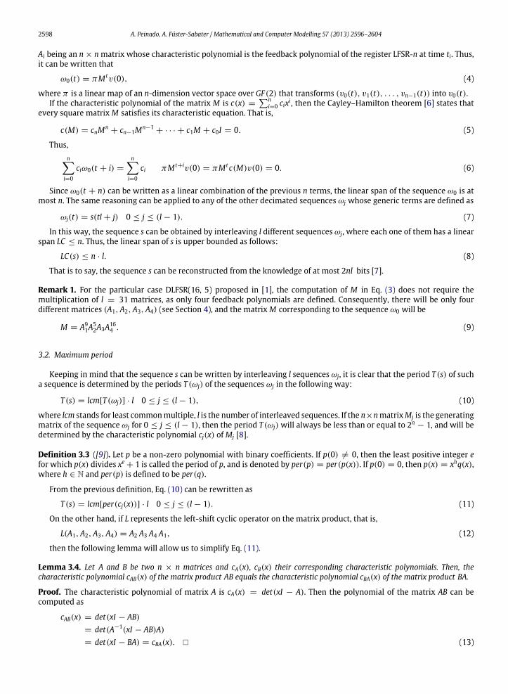
Table 1Selection rules for the feedback primitive polyno-mial in LFSR-16.

Control bits Feedback polynomials

11111 p1(x) = x16 + x15 + x9 + x6 + 101001 p2(x) = x16 + x13 + x9 + x6 + 100001 p3(x) = x16 + x10 + x9 + x6 + 100010 p4(x) = x16 + x12 + x9 + x6 + 1

Fig. 2. PN-sequence generated by control LFSR with feedback polynomial x5 + x3 + 1.

At the same time, it is easy to see that the generating matrices of the decimated sequences ωj satisfy the followingrelationship:

Mj = Lj(M) 0 ≤ j ≤ (l − 1). (14)

For the particular case DLFSR(16, 5), we get

M1 = L1(M) = A81A

52A3A16

4 A1

M2 = L2(M) = A71A

52A3A16

4 A21

...

M9 = L9(M) = A52A3A16

4 A91

...

(15)

Making use of Lemma 3.4, it holds that cj(x) = c(x) for 0 ≤ j ≤ (l − 1). Hence,

T (s) = per(c(x)) · l. (16)

This result shows that the maximum period for any DLFSR configuration is obtained when the polynomial c(x) isprimitive. Thus, the period of s is guaranteed to be T (s) ≤ (2n

− 1) · (2m− 1).

4. An illustrative example: analysis of the DLFSR(16, 5)

The particular implementation proposed in [1] deals with a DLFSR(16, 5) whosemain register LFSR-16 can take up to fourprimitive polynomials andwhose control register LFSR-5 has as feedback polynomial x5 +x3 +1. The control bits that selectthe corresponding feedback polynomial in LFSR-16 are depicted in Table 1. In fact, the control register LFSR-5 generates 31non-zero states while the feedback polynomial in LFSR-16 changes only four times.

Taking the state 11111 (in decimal 31) as the register LFSR-5 seed (initial state), 9 successive states are generated beforegetting the state 01001 (in decimal 9), then other 5 more states until arriving at state 00001 (in decimal 1) which directlyjumps into state 00010 (in decimal 2) and, finally, 16 new states follow the succession until getting again the initial condition.See Fig. 2 for details.

4.1. Linear span

Making use of the inequality (8) and applying it to the DLFSR(16, 5) proposed in [1], we obtain that LC(s) ≤ 16·31 = 496.This value can be easily checked by means of the Massey–Berlekamp algorithm [7]. The obtained LC takes the values 434 or464 for different sequences generated from different initial seeds in the LFSR-16. See Table 2, Fig. 3.

4.2. Maximum period

For the DLFSR(16, 5), the computation of matrix M in Eq. (3) does not require the multiplication of l = 31 differentmatrices as only four feedback polynomials are used. Consequently, there are four different matrices (A1, A2, A3, A4) thatwill be multiplied a number of times according to the state diagram in Fig. 2. In fact, for the sequence ω0, the generatingmatrix is computed as

M = A91A

52A3A16

4 . (17)

2600 A. Peinado, A. Fúster-Sabater / Mathematical and Computer Modelling 57 (2013) 2596–2604

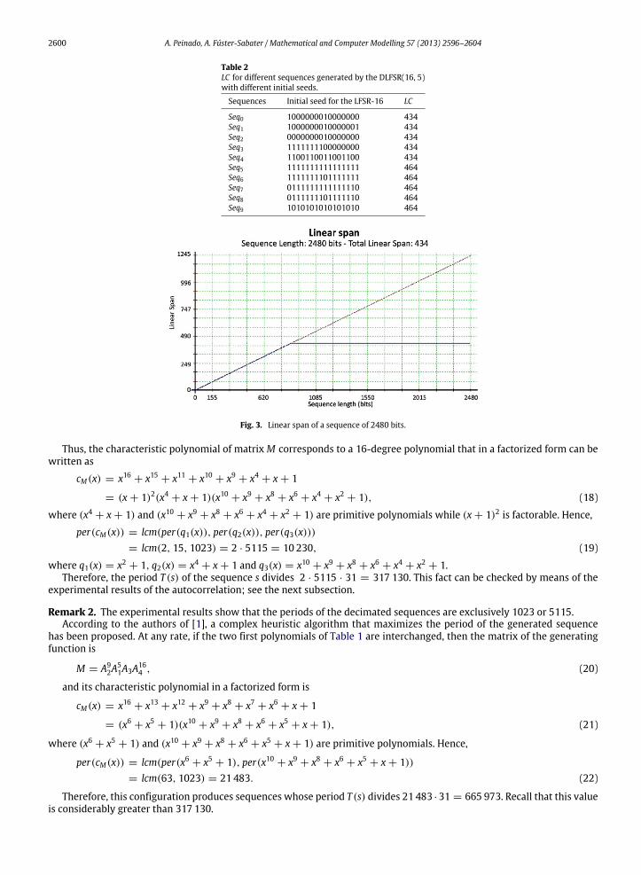
Table 2LC for different sequences generated by the DLFSR(16, 5)with different initial seeds.

Sequences Initial seed for the LFSR-16 LC

Seq0 1000000010000000 434Seq1 1000000010000001 434Seq2 0000000010000000 434Seq3 1111111100000000 434Seq4 1100110011001100 434Seq5 1111111111111111 464Seq6 1111111101111111 464Seq7 0111111111111110 464Seq8 0111111101111110 464Seq9 1010101010101010 464

Fig. 3. Linear span of a sequence of 2480 bits.

Thus, the characteristic polynomial of matrix M corresponds to a 16-degree polynomial that in a factorized form can bewritten as

cM(x) = x16 + x15 + x11 + x10 + x9 + x4 + x + 1

= (x + 1)2(x4 + x + 1)(x10 + x9 + x8 + x6 + x4 + x2 + 1), (18)

where (x4 + x + 1) and (x10 + x9 + x8 + x6 + x4 + x2 + 1) are primitive polynomials while (x + 1)2 is factorable. Hence,

per(cM(x)) = lcm(per(q1(x)), per(q2(x)), per(q3(x)))= lcm(2, 15, 1023) = 2 · 5115 = 10 230, (19)

where q1(x) = x2 + 1, q2(x) = x4 + x + 1 and q3(x) = x10 + x9 + x8 + x6 + x4 + x2 + 1.Therefore, the period T (s) of the sequence s divides 2 · 5115 · 31 = 317 130. This fact can be checked by means of the

experimental results of the autocorrelation; see the next subsection.

Remark 2. The experimental results show that the periods of the decimated sequences are exclusively 1023 or 5115.According to the authors of [1], a complex heuristic algorithm that maximizes the period of the generated sequence

has been proposed. At any rate, if the two first polynomials of Table 1 are interchanged, then the matrix of the generatingfunction is

M = A92A

51A3A16

4 , (20)

and its characteristic polynomial in a factorized form is

cM(x) = x16 + x13 + x12 + x9 + x8 + x7 + x6 + x + 1

= (x6 + x5 + 1)(x10 + x9 + x8 + x6 + x5 + x + 1), (21)

where (x6 + x5 + 1) and (x10 + x9 + x8 + x6 + x5 + x + 1) are primitive polynomials. Hence,

per(cM(x)) = lcm(per(x6 + x5 + 1), per(x10 + x9 + x8 + x6 + x5 + x + 1))= lcm(63, 1023) = 21 483. (22)

Therefore, this configuration produces sequences whose period T (s) divides 21 483 ·31 = 665 973. Recall that this valueis considerably greater than 317130.

A. Peinado, A. Fúster-Sabater / Mathematical and Computer Modelling 57 (2013) 2596–2604 2601

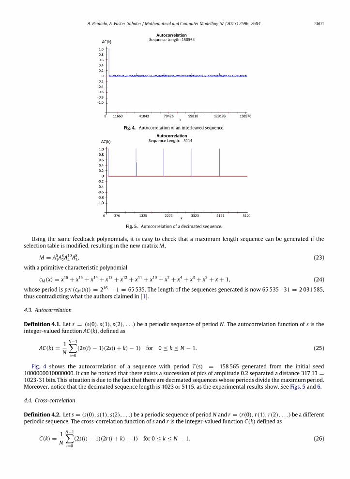
Fig. 4. Autocorrelation of an interleaved sequence.

Fig. 5. Autocorrelation of a decimated sequence.

Using the same feedback polynomials, it is easy to check that a maximum length sequence can be generated if theselection table is modified, resulting in the new matrixM ,

M = A51A

82A

104 A8

3, (23)

with a primitive characteristic polynomial

cM(x) = x16 + x15 + x14 + x13 + x12 + x11 + x10 + x7 + x4 + x3 + x2 + x + 1, (24)

whose period is per(cM(x)) = 216− 1 = 65 535. The length of the sequences generated is now 65 535 · 31 = 2 031 585,

thus contradicting what the authors claimed in [1].

4.3. Autocorrelation

Definition 4.1. Let s = (s(0), s(1), s(2), . . .) be a periodic sequence of period N . The autocorrelation function of s is theinteger-valued function AC(k), defined as

AC(k) =1N

N−1i=0

(2s(i) − 1)(2s(i + k) − 1) for 0 ≤ k ≤ N − 1. (25)

Fig. 4 shows the autocorrelation of a sequence with period T (s) = 158 565 generated from the initial seed1000000010000000. It can be noticed that there exists a succession of pics of amplitude 0.2 separated a distance 317 13 =

1023·31 bits. This situation is due to the fact that there are decimated sequenceswhose periods divide themaximumperiod.Moreover, notice that the decimated sequence length is 1023 or 5115, as the experimental results show. See Figs. 5 and 6.

4.4. Cross-correlation

Definition 4.2. Let s = (s(0), s(1), s(2), . . .) be a periodic sequence of periodN and r = (r(0), r(1), r(2), . . .) be a differentperiodic sequence. The cross-correlation function of s and r is the integer-valued function C(k) defined as

C(k) =1N

N−1i=0

(2s(i) − 1)(2r(i + k) − 1) for 0 ≤ k ≤ N − 1. (26)

2602 A. Peinado, A. Fúster-Sabater / Mathematical and Computer Modelling 57 (2013) 2596–2604

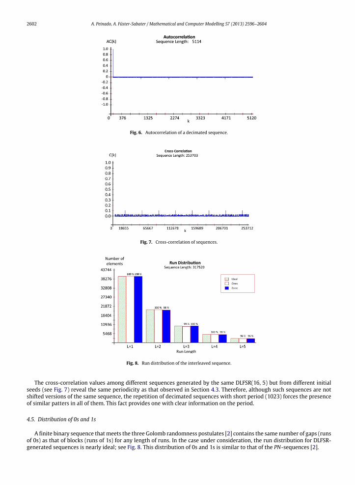
Fig. 6. Autocorrelation of a decimated sequence.

Fig. 7. Cross-correlation of sequences.

Fig. 8. Run distribution of the interleaved sequence.

The cross-correlation values among different sequences generated by the same DLFSR(16, 5) but from different initialseeds (see Fig. 7) reveal the same periodicity as that observed in Section 4.3. Therefore, although such sequences are notshifted versions of the same sequence, the repetition of decimated sequences with short period (1023) forces the presenceof similar patters in all of them. This fact provides one with clear information on the period.

4.5. Distribution of 0s and 1s

A finite binary sequence thatmeets the three Golomb randomness postulates [2] contains the same number of gaps (runsof 0s) as that of blocks (runs of 1s) for any length of runs. In the case under consideration, the run distribution for DLFSR-generated sequences is nearly ideal; see Fig. 8. This distribution of 0s and 1s is similar to that of the PN-sequences [2].

A. Peinado, A. Fúster-Sabater / Mathematical and Computer Modelling 57 (2013) 2596–2604 2603

5. Interleaved sequence model for the DLFSR

In [10], Gong introduced the concept of an interleaved sequence whose period, linear span, linear equivalent, andautocorrelation could be easily computed. The importance of this kind of sequence derives from the fact that many well-known pseudorandom cryptographic sequences (e.g. Gold sequence family, Kasami (small and large set) sequence families,GMW sequences, Klapper sequences, No sequences, etc. [3]) are included in the class of interleaved sequences. Thus, theresults introduced in [10] can be applied to all of them. In this way, a large number of pseudorandom sequence generatorscan be studied by using a unique theoretical model; see also [11–14].

According to [10], interleaved sequences are defined over GF(q), that is, a more general Galois field than the binary casewhere q is a prime number. A formal definition of interleaved sequence is as follows.

Definition 5.1 (See [10, Definition 1]). Let f (x) be a polynomial over GF(q) of degree n with f (0) = 0, and let l be a positiveinteger. For any sequence u = (u(0), u(1), u(2), . . .) = (u(t)) over GF(q), write k = tl + j (t = 0, 1, 2, . . . j =

0, 1, . . . , (l − 1)). If the decimated sequences uj = (u(tl + j)) t ≥ 0 are generated by f (x) for all j, then u is called aninterleaved sequence over GF(q) of size l associated with f (x).

The decimated sequences uj are also called the component sequences of the interleaved sequence.At the same time, in [10], the upper bound on the period and linear span of interleaved sequences is established via the

following lemma.

Lemma 5.2 (See [10, Lemma 1]). Let u be an interleaved sequence defined over GF(q) of size l associated with f (x). In addition,let h(x) be the minimal polynomial of u over GF(q). Then, the following hold.

1. The minimal polynomial h(x) of u satisfies h(x)|f (xl), so that the linear span of the interleaved sequence (the degree of itsminimal polynomial) is upper bound by LC(u) ≤ nl.

2. T (u)|per(f )l, where T (u) is the period of the sequence u and per(f ) the period of the polynomial f .

Next, we can see how the sequences generated from a DLFSR generator can be considered as interleaved sequences inthe sense given in Definition 5.1. In order to accomplish this task, it suffices to apply the same computation method usedin Section 3. Indeed, the sequence s generated by the DLFSR(16, 5) can be decomposed as l = 25

− 1 = 31 sequences ωj(t)obtained by decimation of s taking one bit out of 31. That is,

ωj = s(tl + j) (27)

with j = 0, 1, . . . , (l − 1) and l = 31. Each one of these sequences is generated by a matrix Mj computed from thematrices Aj corresponding to each one of the feedback polynomials in the assignment table of the DLFSR generator. Asit was proved in Section 3, all the matrices Mj have the same characteristic polynomial, notated cM(x), that generates allthe decimated sequences ωj. Therefore, according to Definition 5.1, the sequences generated by the DLFSR generator areinterleaved sequences over GF(2) of size l = 31 and associated with f (x) = cM(x).

Thus, making use of Lemma 5.2, it can be concluded that the sequences generated by the DLFSR(16, 5) have a linear spanLC(s) ≤ nl = n(2m

− 1) = 16 · 31 = 496. Recall that the upper bound equals that obtained in Section 4. On the other hand,Lemma 3.4 proves that the period T (s) of the DLFSR sequences divides per(cM(x)) · l. From Eqs. (17)–(18), it can be deducedthat the period T (s) of the sequence s divides 10 230 · 31 = 317 130 such as was computed in Section 4.

Finally, it must be noticed that the characteristic polynomial cM(x) that generates all the decimated sequences ωjis not irreducible. Thus, the DLFSR sequences belong neither to the class of interleaved sequences called IRI-sequences(IRreducible Interleaved sequences [10]) nor to the class of interleaved sequences called PI-sequences (Primitive Interleavedsequences [10]). Both classes (IRI-sequences and PI-sequences) have been studied by Gong, and they exhibit the mostsuitable properties for their practical application. At present, the question that arises in a natural way is: is it possibleto design a DLFSR(n,m) generator whose characteristic polynomial cM(x) is primitive or at least irreducible? In general, theanswer seems to be complex. Simulations and theoretical studies consider that the probability of finding a solution to thisproblem tends to zero as far as n increases [6]. In spite of that, the characterization of the solution set is now in progress.

5.1. A method to reconstruct sequences generated by DLFSRs

Taking into account that the upper bound for the linear span is LC(s) ≤ nl = n · (2m− 1), the most immediate method

to reconstruct the whole sequence is the application of the Massey–Berlekamp algorithm [7]. That is, we only need 2nl bitsof s to get an LFSR of length nl that is able to generate the sequence from the first nl bits.

In the particular case of the DLFSR(16, 5) originally proposed in [1], 2nl = 992 bits are needed. They will be the input totheMassey–Berlekamp algorithm to determine an LFSR of length≤ 496 and its correspondingminimal polynomial, notatedf (x). From these 496 bits and the LFSR, the whole sequence can be reconstructed.

Nevertheless, keeping in mind that the sequence s is made by interleaving l sequences ωj, all of them generated by thesame matrixM (see Eq. (3)), the following method to reconstruct s can be given.

2604 A. Peinado, A. Fúster-Sabater / Mathematical and Computer Modelling 57 (2013) 2596–2604

1. Take 2nl bits of the sequence s.2. Construct the component sequences ωj by decimation of s; that is,

ωj(t) = s(tl + j) t ≥ 0. (28)3. Compute theminimal polynomial that generates each sequenceωj via theMassey–Berlekamp algorithm by using 2n bits

of ωj.4. From the minimal polynomials fj(x) of each sequence ωj, the l decimated sequences can be reconstructed in parallel.

Then, the interleaving of all these sequences makes the whole sequence s.

Remark 3. This method allows one to obtain parallelization in the computation of the linear span. In this way, the sequencereconstruction problem can be faced even for large values of the linear span.

Remark 4. As expected, the minimal polynomials of the sequences ωj coincide with the factors of the characteristicpolynomial of matrixM .

On the other hand, Lemma 5.2 allows one to reconstruct the sequence s in an easy way, provided that the parameterl is known. Recall that the knowledge of the control sequence is not needed, just its length. The successive steps of thereconstruction procedure are as follows.1. Construct one of the decimated sequences.2. Compute its minimal polynomialm(x) via the Massey–Berlekamp algorithm.3. If m(x) = f (x), then the minimal polynomial of the sequence s will be h(x) = f (xl), as stated in Lemma 5.2. Otherwise,

m(xl) will generate a different sequence. In that case, a k-error linear complexity method should be used in order toanalyze the divergence.

6. Conclusions

Due mainly to the detected correlation features, it can be concluded that the use of DLFSR sequences in cryptographic orCDMA communications is not recommended.1. Concerning cryptographic application, it must be noticed that the upper bound of the linear span is independent of the

polynomial table considered. That is, this value is independent of the number of feedback polynomials for the mainregister LFSR-n as well as of the assignment of states for the control register LFSR-m. Moreover, this upper bound is alsoindependent of the PN-sequence generated by the register LFSR-m. In fact, it depends only on its length. Thus, this resultcan be applied to any DLFSR generator that preserves the number of stages in the control register LFSR-m.

In order to apply the DLFSR scheme to real systems, in which a large period and a linear span of about half a periodare recommended, it can be said that it is difficult to find a configuration with arbitrary values of the parameters thatmaintains a good level of quality for the generated sequences.

2. Concerning the application in CDMA communications, the results obtained over the original proposal in [1] revealcorrelation values that are not adequate for their use in CDMA communications.

An extension of this article, which is part of work in progress, is the analysis of DLFSR generatorswhose sequences belongto the class of PI-sequences.

Acknowledgments

This work was supported in part by CDTI (Spain) and the companies INDRA, Unión Fenosa, Tecnobit, Visual Tools,Brainstorm, SAC and Technosafe under Project Cenit-HESPERIA; by Ministry of Science and Innovation and European FEDERFund under Project TIN2008-02236/TSI.

References

[1] R. Mita, G. Palumbo, S. Pennisi, M. Poli, Pseudorandom bit generator based on dynamic linear feedback topology, Electron. Lett. 38 (2002) 1097–1098.[2] S.W. Golomb, Shift-Register Sequences, revised edition, Aegean Park Press, Laguna Hill, California, 1982.[3] R. Rueppel, Stream Ciphers, in: Gustavus J. Simmons (Ed.), Contemporary Cryptology, The Science of Information, IEEE Press, 1992, pp. 65–134.[4] S. Blackburn, S. Murphy, K. Paterson, Comments on theory and applications of cellular automata to cryptography, IEEE Trans. Comput. 46 (1997)

637–638.[5] A. Fúster-Sabater, P. Caballero-Gil, Cellular automata in cryptanalysis of stream ciphers, in: Proc. of ACRI 2006, in: Lecture Notes in Computer Science,

Springer-Verlag, Berlin, Germany, 2006, pp. 611–616.[6] J. Muñoz, A. Peinado, On the characteristic polynomial of the product of matrices with irreducible characteristic polynomials, Technical Report

UMA-IC03-A0-002, 2003.[7] J.L. Massey, Shift register synthesis and BCH decoding, IEEE Trans. Inform. Theory 15 (1969) 122–127.[8] P.P. Chaudhuri, D.R. Chowdhury, S. Nandi, S. Chattopadhyay, Additive Cellular Automata, Theory and Applications, IEEE Computer Society, 1997.[9] R. Lidl, H. Niederreiter, Finite Fields, Cambridge University Press, 1996.

[10] G. Gong, Theory and applications of q-ary interleaved sequences, IEEE Trans. Inform. Theory 41 (1995) 400–411.[11] A. Fúster-Sabater, P. Caballero-Gil, Synthesis of cryptographic interleaved sequences by means of linear cellular automata, Appl. Math. Lett. 22 (2009)

1518–1524.[12] H. Hu, G. Gong, New sets of zero or low correlation zone sequences via interleaving techniques, IEEE Trans. Inform. Theory 56 (2010) 1702–1713.[13] S. Jiang, Z. Dai, G. Gong, On interleaved sequences over finite fields, Discrete Math. 252 (2002) 161–178.[14] Z. Zhou, X. Tang, G. Gong, A new class of sequences with zero or low correlation zone based on interleaving technique, IEEE Trans. Inform. Theory 54

(2008) 4267–4273.