generating loop invariants via polynomial...
TRANSCRIPT
Generating Loop Invariants via PolynomialInterpolation
Marc Moreno MazaJoint work with
Rong Xiao
University of Western Ontario, Canada
East China Normal UniversityMay 24, 2012
Plan
1 PreliminariesNotions on loop invariantsPoly-geometric summationsA variation on Bezout’s Theorem
2 Invariant ideal of P -solvable recurrencesDegree estimates for solutions of P -solvable recurrencesP -solvable recurrencesDegree estimates for solutions of P -solvable recurrencesDegree estimates for their invariant idealDimension estimates for their invariant ideal
3 Loop invariant generation via polynomial interpolationA direct approachA modular methodExperimentationMaple Package: ProgramAnalysis

Preliminaries Notions on loop invariants
Plan
1 PreliminariesNotions on loop invariantsPoly-geometric summationsA variation on Bezout’s Theorem
2 Invariant ideal of P -solvable recurrencesDegree estimates for solutions of P -solvable recurrencesP -solvable recurrencesDegree estimates for solutions of P -solvable recurrencesDegree estimates for their invariant idealDimension estimates for their invariant ideal
3 Loop invariant generation via polynomial interpolationA direct approachA modular methodExperimentationMaple Package: ProgramAnalysis
Preliminaries Notions on loop invariants
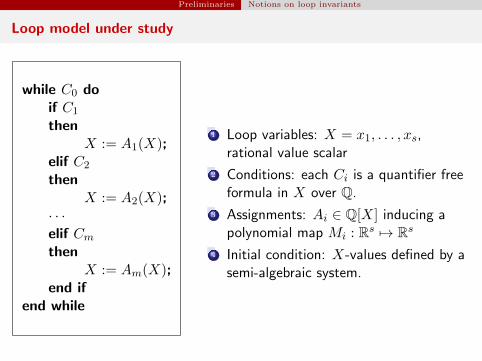
Loop model under study
while C0 doif C1
thenX := A1(X);
elif C2
thenX := A2(X);
· · ·elif Cmthen
X := Am(X);end if
end while
1 Loop variables: X = x1, . . . , xs,rational value scalar
2 Conditions: each Ci is a quantifier freeformula in X over Q.
3 Assignments: Ai ∈ Q[X] inducing apolynomial map Mi : Rs 7→ Rs
4 Initial condition: X-values defined by asemi-algebraic system.
Preliminaries Notions on loop invariants
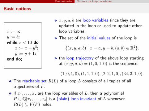
Basic notions
x := a;y := b;while x < 10 do
x := x+ y5;y := y + 1;
end do;
x, y, a, b are loop variables since they areupdated in the loop or used to update otherloop variables.
The set of the initial values of the loop is
{(x, y, a, b) | x = a, y = b, (a, b) ∈ R2}.
the loop trajectory of the above loop startingat (x, y, a, b) = (1, 0, 1, 0) is the sequence:
(1, 0, 1, 0), (1, 1, 1, 0), (2, 2, 1, 0), (34, 3, 1, 0).
The reachable set R(L) of a loop L consists of all tuples of alltrajectories of L.
If x1, . . . , xs are the loop variables of L, then a polynomialP ∈ Q[x1, . . . , xs] is a (plain) loop invariant of L wheneverR(L) ⊆ V (P ) holds.
Preliminaries Notions on loop invariants
More notions
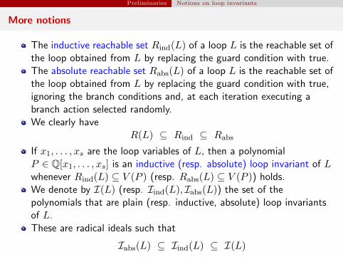
The inductive reachable set Rind(L) of a loop L is the reachable set ofthe loop obtained from L by replacing the guard condition with true.The absolute reachable set Rabs(L) of a loop L is the reachable set ofthe loop obtained from L by replacing the guard condition with true,ignoring the branch conditions and, at each iteration executing abranch action selected randomly.We clearly have
R(L) ⊆ Rind ⊆ Rabs
If x1, . . . , xs are the loop variables of L, then a polynomialP ∈ Q[x1, . . . , xs] is an inductive (resp. absolute) loop invariant of Lwhenever Rind(L) ⊆ V (P ) (resp. Rabs(L) ⊆ V (P )) holds.We denote by I(L) (resp. Iind(L), Iabs(L)) the set of thepolynomials that are plain (resp. inductive, absolute) loop invariantsof L.These are radical ideals such that
Iabs(L) ⊆ Iind(L) ⊆ I(L)
Preliminaries Notions on loop invariants
Absolute invariants might be trivial
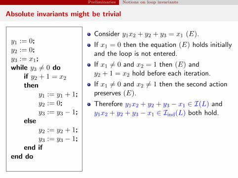
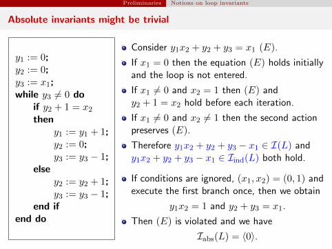
y1 := 0;y2 := 0;y3 := x1;while y3 6= 0 do
if y2 + 1 = x2then
y1 := y1 + 1;y2 := 0;y3 := y3 − 1;
elsey2 := y2 + 1;y3 := y3 − 1;
end ifend do
Consider y1x2 + y2 + y3 = x1 (E).
If x1 = 0 then the equation (E) holds initiallyand the loop is not entered.
If x1 6= 0 and x2 = 1 then (E) andy2 + 1 = x2 hold before each iteration.
If x1 6= 0 and x2 6= 1 then the second actionpreserves (E).
Therefore y1x2 + y2 + y3 − x1 ∈ I(L) andy1x2 + y2 + y3 − x1 ∈ Iind(L) both hold.
If conditions are ignored, (x1, x2) = (0, 1) andexecute the first branch once, then we obtain
y1x2 = 1 and y2 + y3 = x1.
Then (E) is violated and we have
Iabs(L) = 〈0〉.
Preliminaries Notions on loop invariants
Absolute invariants might be trivial
y1 := 0;y2 := 0;y3 := x1;while y3 6= 0 do
if y2 + 1 = x2then
y1 := y1 + 1;y2 := 0;y3 := y3 − 1;
elsey2 := y2 + 1;y3 := y3 − 1;
end ifend do
Consider y1x2 + y2 + y3 = x1 (E).
If x1 = 0 then the equation (E) holds initiallyand the loop is not entered.
If x1 6= 0 and x2 = 1 then (E) andy2 + 1 = x2 hold before each iteration.
If x1 6= 0 and x2 6= 1 then the second actionpreserves (E).
Therefore y1x2 + y2 + y3 − x1 ∈ I(L) andy1x2 + y2 + y3 − x1 ∈ Iind(L) both hold.
If conditions are ignored, (x1, x2) = (0, 1) andexecute the first branch once, then we obtain
y1x2 = 1 and y2 + y3 = x1.
Then (E) is violated and we have
Iabs(L) = 〈0〉.
Preliminaries Notions on loop invariants
Inductive invariants might not be plain invariants
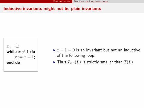
x := 1;while x 6= 1 do
x := x+ 1;end do
x− 1 = 0 is an invariant but not an inductiveof the following loop.
Thus Iind(L) is strictly smaller than I(L)
Preliminaries Notions on loop invariants
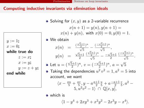
Computing inductive invariants via elimination ideals
y := 1;x := 0;while true do
z := x;x := y;y := z + y;
end while
Solving for (x, y) as a 2-variable recurrence
x(n+ 1) = y(n), y(n+ 1) =x(n) + y(n), with x(0) = 0, y(0) = 1.
We obtain
x(n) =(√5+12
)n√5− (−
√5+12
)n√5
,
y(n) =√5+12
(√5+12
)n√5− −
√5+12
(−√5+12
)n√5
.
Let u = (√5+12 )n, v = (−
√5+12 )n, a =
√5
Taking the dependencies u2 v2 = 1, a2 = 5 intoaccount, we want
〈x− au5 + av
5 , y − aa+12
u5 + a−a+1
2v5 , a
2 −5, u2v2 − 1〉 ∩ Q[x, y],
which is
〈1− y4 + 2xy3 + x2y2 − 2x3y − x4〉.
Preliminaries Notions on loop invariants
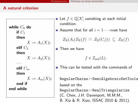
A natural criterion
while C0 doif C1
thenX := A1(X);
elif C2
thenX := A2(X);
· · ·elif Cmthen
X := Am(X);end if
end while
Let f ∈ Q[X] vanishing at each initialcondition.
Assume that for all i = 1 · · ·mwe have
ZR(Ai(ZR(f) ∩ ZR(Ci))) ⊆ ZR(f)
Then we have
f ∈ Iind(L).
This can be tested with the commands of
RegularChains:-SemiAlgebraicSetTools
based on theRegularChains:-RealTriangularize
(C. Chen, J.H. Davenport, M.M.M.,B. Xia & R. Xiao, ISSAC 2010 & 2011).

Preliminaries Notions on loop invariants
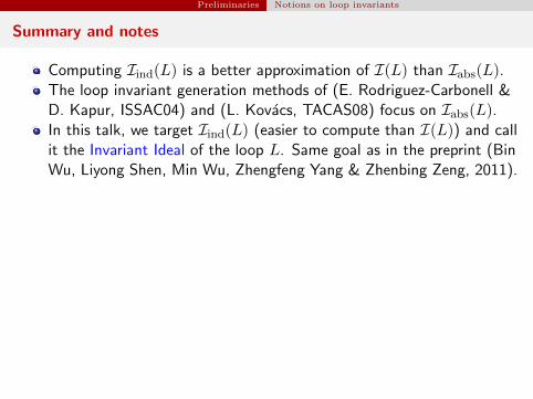
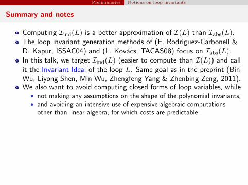
Summary and notes
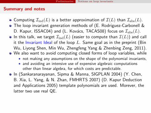
Computing Iind(L) is a better approximation of I(L) than Iabs(L).The loop invariant generation methods of (E. Rodriguez-Carbonell &D. Kapur, ISSAC04) and (L. Kovacs, TACAS08) focus on Iabs(L).
In this talk, we target Iind(L) (easier to compute than I(L)) and callit the Invariant Ideal of the loop L. Same goal as in the preprint (BinWu, Liyong Shen, Min Wu, Zhengfeng Yang & Zhenbing Zeng, 2011).We also want to avoid computing closed forms of loop variables, while
• not making any assumptions on the shape of the polynomial invariants,• and avoiding an intensive use of expensive algebraic computations
other than linear algebra, for which costs are predictable.
In (Sankaranarayanan, Sipma & Manna, SIGPLAN 2004) (Y. Chen,B. Xia, L. Yang, & N. Zhan, FMHRTS 2007) (D. Kapur Deductionand Applications 2005) template polynomials are used. Morever, thelatter two use real QE.The ”abstract interpretation” method (E. Rodriguez-Carbonell & D.Kapur, Science of Computer Programming 2007) does not usetemplates but uses of Grobner bases heavily.
Preliminaries Notions on loop invariants
Summary and notes
Computing Iind(L) is a better approximation of I(L) than Iabs(L).The loop invariant generation methods of (E. Rodriguez-Carbonell &D. Kapur, ISSAC04) and (L. Kovacs, TACAS08) focus on Iabs(L).In this talk, we target Iind(L) (easier to compute than I(L)) and callit the Invariant Ideal of the loop L. Same goal as in the preprint (BinWu, Liyong Shen, Min Wu, Zhengfeng Yang & Zhenbing Zeng, 2011).
We also want to avoid computing closed forms of loop variables, while• not making any assumptions on the shape of the polynomial invariants,• and avoiding an intensive use of expensive algebraic computations
other than linear algebra, for which costs are predictable.
In (Sankaranarayanan, Sipma & Manna, SIGPLAN 2004) (Y. Chen,B. Xia, L. Yang, & N. Zhan, FMHRTS 2007) (D. Kapur Deductionand Applications 2005) template polynomials are used. Morever, thelatter two use real QE.The ”abstract interpretation” method (E. Rodriguez-Carbonell & D.Kapur, Science of Computer Programming 2007) does not usetemplates but uses of Grobner bases heavily.
Preliminaries Notions on loop invariants
Summary and notes
Computing Iind(L) is a better approximation of I(L) than Iabs(L).The loop invariant generation methods of (E. Rodriguez-Carbonell &D. Kapur, ISSAC04) and (L. Kovacs, TACAS08) focus on Iabs(L).In this talk, we target Iind(L) (easier to compute than I(L)) and callit the Invariant Ideal of the loop L. Same goal as in the preprint (BinWu, Liyong Shen, Min Wu, Zhengfeng Yang & Zhenbing Zeng, 2011).We also want to avoid computing closed forms of loop variables, while
• not making any assumptions on the shape of the polynomial invariants,• and avoiding an intensive use of expensive algebraic computations
other than linear algebra, for which costs are predictable.
In (Sankaranarayanan, Sipma & Manna, SIGPLAN 2004) (Y. Chen,B. Xia, L. Yang, & N. Zhan, FMHRTS 2007) (D. Kapur Deductionand Applications 2005) template polynomials are used. Morever, thelatter two use real QE.The ”abstract interpretation” method (E. Rodriguez-Carbonell & D.Kapur, Science of Computer Programming 2007) does not usetemplates but uses of Grobner bases heavily.
Preliminaries Notions on loop invariants
Summary and notes
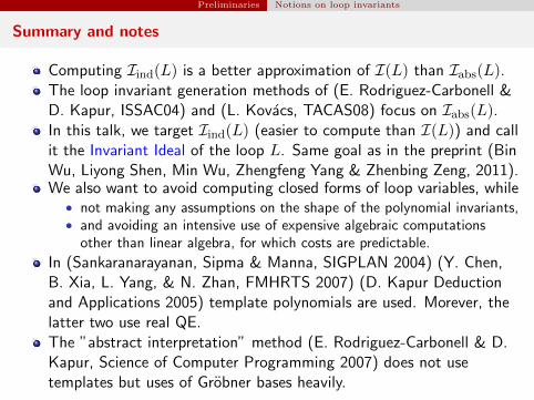
Computing Iind(L) is a better approximation of I(L) than Iabs(L).The loop invariant generation methods of (E. Rodriguez-Carbonell &D. Kapur, ISSAC04) and (L. Kovacs, TACAS08) focus on Iabs(L).In this talk, we target Iind(L) (easier to compute than I(L)) and callit the Invariant Ideal of the loop L. Same goal as in the preprint (BinWu, Liyong Shen, Min Wu, Zhengfeng Yang & Zhenbing Zeng, 2011).We also want to avoid computing closed forms of loop variables, while
• not making any assumptions on the shape of the polynomial invariants,• and avoiding an intensive use of expensive algebraic computations
other than linear algebra, for which costs are predictable.
In (Sankaranarayanan, Sipma & Manna, SIGPLAN 2004) (Y. Chen,B. Xia, L. Yang, & N. Zhan, FMHRTS 2007) (D. Kapur Deductionand Applications 2005) template polynomials are used. Morever, thelatter two use real QE.
The ”abstract interpretation” method (E. Rodriguez-Carbonell & D.Kapur, Science of Computer Programming 2007) does not usetemplates but uses of Grobner bases heavily.
Preliminaries Notions on loop invariants
Summary and notes
Computing Iind(L) is a better approximation of I(L) than Iabs(L).The loop invariant generation methods of (E. Rodriguez-Carbonell &D. Kapur, ISSAC04) and (L. Kovacs, TACAS08) focus on Iabs(L).In this talk, we target Iind(L) (easier to compute than I(L)) and callit the Invariant Ideal of the loop L. Same goal as in the preprint (BinWu, Liyong Shen, Min Wu, Zhengfeng Yang & Zhenbing Zeng, 2011).We also want to avoid computing closed forms of loop variables, while
• not making any assumptions on the shape of the polynomial invariants,• and avoiding an intensive use of expensive algebraic computations
other than linear algebra, for which costs are predictable.
In (Sankaranarayanan, Sipma & Manna, SIGPLAN 2004) (Y. Chen,B. Xia, L. Yang, & N. Zhan, FMHRTS 2007) (D. Kapur Deductionand Applications 2005) template polynomials are used. Morever, thelatter two use real QE.The ”abstract interpretation” method (E. Rodriguez-Carbonell & D.Kapur, Science of Computer Programming 2007) does not usetemplates but uses of Grobner bases heavily.

Preliminaries Poly-geometric summations
Plan
1 PreliminariesNotions on loop invariantsPoly-geometric summationsA variation on Bezout’s Theorem
2 Invariant ideal of P -solvable recurrencesDegree estimates for solutions of P -solvable recurrencesP -solvable recurrencesDegree estimates for solutions of P -solvable recurrencesDegree estimates for their invariant idealDimension estimates for their invariant ideal
3 Loop invariant generation via polynomial interpolationA direct approachA modular methodExperimentationMaple Package: ProgramAnalysis
Preliminaries Poly-geometric summations
Poly-geometrical expression
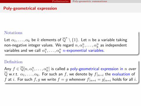
Notations
Let α1, . . . , αk be k elements of Q∗ \ {1}. Let n be a variable takingnon-negative integer values. We regard n, αn1 , . . . , α
nk as independent
variables and we call αn1 , . . . , αnk n-exponential variables.
Definition
Any f ∈ Q[n, αn1 , . . . , αnk ] is called a poly-geometrical expression in n over
Q w.r.t. α1, . . . , αk. For such an f , we denote by f |n=i the evaluation off at i. For such f, g we write f = g whenever f |n=i = g|n=i holds for all i.
Preliminaries Poly-geometric summations
Canonical form of a poly-geometrical expression
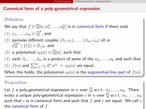
Definition
We say that f ∈ Q[n, αn1 , . . . , αnk ] is in canonical form if there exist
(1) c1, . . . , cm ∈ Q∗, and
(2) pairwise different couples (β1, e1), . . . , (βm, em) all in(Q∗ \ {1})× Z≥0, and
(3) a polynomial c0(n) ∈ Q[n], such that
(4) each β1, . . . , βm is a product of some of the α1, . . . , αk and such that
(5) f(n) and∑m
i=1 ci βni n
ei + c0(n) are equal.
When this holds, the polynomial c0(n) is the exponential-free part of f(n).
Proposition
Let f a poly-geometrical expression in n over Q w.r.t. α1, . . . , αk. Thereexists a unique poly-geometrical expression c in n over Q w.r.t. α1, . . . , αksuch that c is in canonical form and such that f and c are equal. We call cthe canonical form of f .
Preliminaries Poly-geometric summations
Examples of poly-geometrical expressions
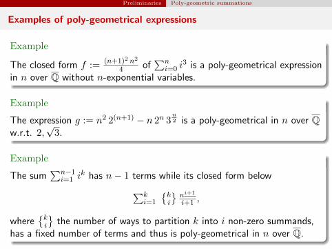
Example
The closed form f := (n+1)2 n2
4 of∑n
i=0 i3 is a poly-geometrical expression
in n over Q without n-exponential variables.
Example
The expression g := n2 2(n+1) − n 2n 3n2 is a poly-geometrical in n over Q
w.r.t. 2,√
3.
Example
The sum∑n−1
i=1 ik has n− 1 terms while its closed form below∑k
i=1
{ki
}ni+1
i+1 ,
where{ki
}the number of ways to partition k into i non-zero summands,
has a fixed number of terms and thus is poly-geometrical in n over Q.
Preliminaries Poly-geometric summations
Multiplicative relation ideal
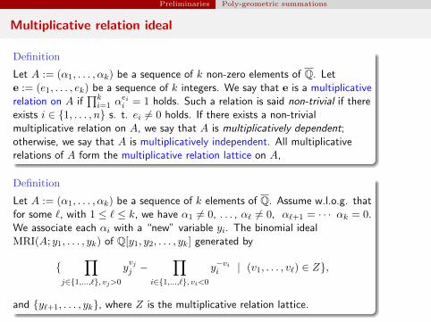
Definition
Let A := (α1, . . . , αk) be a sequence of k non-zero elements of Q. Lete := (e1, . . . , ek) be a sequence of k integers. We say that e is a multiplicativerelation on A if
∏ki=1 α
eii = 1 holds. Such a relation is said non-trivial if there
exists i ∈ {1, . . . , n} s. t. ei 6= 0 holds. If there exists a non-trivialmultiplicative relation on A, we say that A is multiplicatively dependent;otherwise, we say that A is multiplicatively independent. All multiplicativerelations of A form the multiplicative relation lattice on A,
Definition
Let A := (α1, . . . , αk) be a sequence of k elements of Q. Assume w.l.o.g. thatfor some `, with 1 ≤ ` ≤ k, we have α1 6= 0, . . . , α` 6= 0, α`+1 = · · · αk = 0.We associate each αi with a “new” variable yi. The binomial idealMRI(A; y1, . . . , yk) of Q[y1, y2, . . . , yk] generated by
{∏
j∈{1,...,`}, vj>0
yvjj −
∏i∈{1,...,`}, vi<0
y−vii | (v1, . . . , v`) ∈ Z},
and {y`+1, . . . , yk}, where Z is the multiplicative relation lattice.
Preliminaries Poly-geometric summations
Multiplicative relation ideal: example
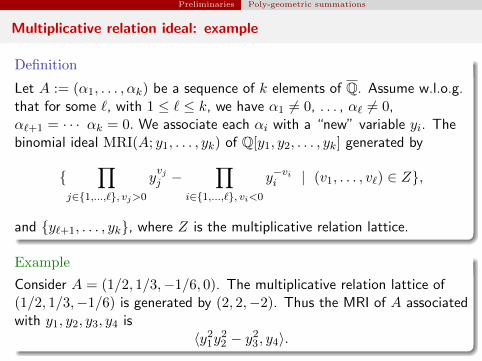
Definition
Let A := (α1, . . . , αk) be a sequence of k elements of Q. Assume w.l.o.g.that for some `, with 1 ≤ ` ≤ k, we have α1 6= 0, . . . , α` 6= 0,α`+1 = · · · αk = 0. We associate each αi with a “new” variable yi. Thebinomial ideal MRI(A; y1, . . . , yk) of Q[y1, y2, . . . , yk] generated by
{∏
j∈{1,...,`}, vj>0
yvjj −
∏i∈{1,...,`}, vi<0
y−vii | (v1, . . . , v`) ∈ Z},
and {y`+1, . . . , yk}, where Z is the multiplicative relation lattice.
Example
Consider A = (1/2, 1/3,−1/6, 0). The multiplicative relation lattice of(1/2, 1/3,−1/6) is generated by (2, 2,−2). Thus the MRI of A associatedwith y1, y2, y3, y4 is
〈y21y22 − y23, y4〉.
Preliminaries Poly-geometric summations
Weak multiplicative independence
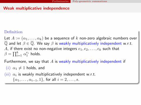
Definition
Let A := (α1, . . . , αk) be a sequence of k non-zero algebraic numbers overQ and let β ∈ Q. We say β is weakly multiplicatively independent w.r.t.A, if there exist no non-negative integers e1, e2, . . . , ek such thatβ =
∏ki=1 α
ei1 holds.
Furthermore, we say that A is weakly multiplicatively independent if
(i) α1 6= 1 holds, and
(ii) αi is weakly multiplicatively independent w.r.t.{α1, . . . , αi−1, 1}, for all i = 2, . . . , s.
Preliminaries Poly-geometric summations
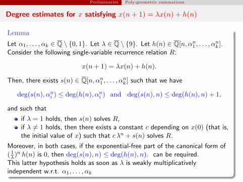
Degree estimates for x satisfying x(n+ 1) = λx(n) + h(n)
Lemma
Let α1, . . . , αk ∈ Q \ {0, 1}. Let λ ∈ Q \ {9}. Let h(n) ∈ Q[n, αn1 , . . . , αnk ].
Consider the following single-variable recurrence relation R:
x(n+ 1) = λx(n) + h(n).
Then, there exists s(n) ∈ Q[n, αn1 , . . . , αnk ] such that we have
deg(s(n), αni ) ≤ deg(h(n), αni ) and deg(s(n), n) ≤ deg(h(n), n) + 1,
and such that
if λ = 1 holds, then s(n) solves R,if λ 6= 1 holds, then there exists a constant c depending on x(0) (that is,the initial value of x) such that c λn + s(n) solves R.
Moreover, in both cases, if the exponential-free part of the canonical form of( 1λ)n h(n) is 0, then deg(s(n), n) ≤ deg(h(n), n). can be required.
This latter hypothesis holds as soon as λ is weakly multiplicativelyindependent w.r.t. α1, . . . , αk

Preliminaries A variation on Bezout’s Theorem
Plan
1 PreliminariesNotions on loop invariantsPoly-geometric summationsA variation on Bezout’s Theorem
2 Invariant ideal of P -solvable recurrencesDegree estimates for solutions of P -solvable recurrencesP -solvable recurrencesDegree estimates for solutions of P -solvable recurrencesDegree estimates for their invariant idealDimension estimates for their invariant ideal
3 Loop invariant generation via polynomial interpolationA direct approachA modular methodExperimentationMaple Package: ProgramAnalysis
Preliminaries A variation on Bezout’s Theorem
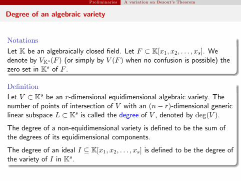
Degree of an algebraic variety
Notations
Let K be an algebraically closed field. Let F ⊂ K[x1, x2, . . . , xs]. Wedenote by VKs(F ) (or simply by V (F ) when no confusion is possible) thezero set in Ks of F .
Definition
Let V ⊂ Ks be an r-dimensional equidimensional algebraic variety. Thenumber of points of intersection of V with an (n− r)-dimensional genericlinear subspace L ⊂ Ks is called the degree of V , denoted by deg(V ).
The degree of a non-equidimensional variety is defined to be the sum ofthe degrees of its equidimensional components.
The degree of an ideal I ⊆ K[x1, x2, . . . , xs] is defined to be the degree ofthe variety of I in Ks.
Preliminaries A variation on Bezout’s Theorem
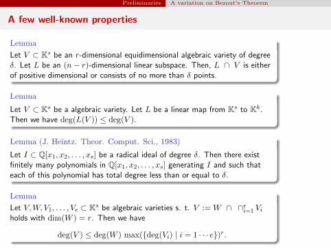
A few well-known properties
Lemma
Let V ⊂ Ks be an r-dimensional equidimensional algebraic variety of degreeδ. Let L be an (n− r)-dimensional linear subspace. Then, L ∩ V is eitherof positive dimensional or consists of no more than δ points.
Lemma
Let V ⊂ Ks be a algebraic variety. Let L be a linear map from Ks to Kk.Then we have deg(L(V )) ≤ deg(V ).
Lemma (J. Heintz. Theor. Comput. Sci., 1983)
Let I ⊂ Q[x1, x2, . . . , xs] be a radical ideal of degree δ. Then there existfinitely many polynomials in Q[x1, x2, . . . , xs] generating I and such thateach of this polynomial has total degree less than or equal to δ.
Lemma
Let V,W, V1, . . . , Ve ⊂ Ks be algebraic varieties s. t. V := W ∩ ∩ei=1 Viholds with dim(W ) = r. Then we have
deg(V ) ≤ deg(W ) max({deg(Vi) | i = 1 · · · e})r.
Preliminaries A variation on Bezout’s Theorem
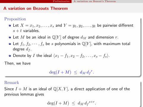
A variation on Bezouts Theorem
Proposition
Let X = x1, x2, . . . , xs and Y = y1, y2, . . . , yt be pairwise differents+ t variables.
Let M be an ideal in Q[Y ] of degree dM and dimension r.
Let f1, f2, · · · , fs be s polynomials in Q[Y ], with maximum totaldegree df .
Denote by I the ideal 〈x1 − f1, x2 − f2, . . . , xs − fs〉.
Then, we have
deg(I +M) ≤ dM dfr.
Remark
Since I +M is an ideal of Q[X,Y ], a direct application of one of theprevious lemmas gives
deg(I +M) ≤ dM dfs+r.
Preliminaries A variation on Bezout’s Theorem
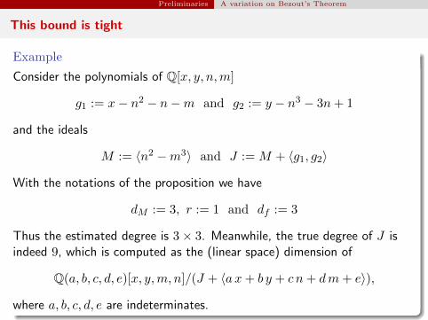
This bound is tight
Example
Consider the polynomials of Q[x, y, n,m]
g1 := x− n2 − n−m and g2 := y − n3 − 3n+ 1
and the ideals
M := 〈n2 −m3〉 and J := M + 〈g1, g2〉
With the notations of the proposition we have
dM := 3, r := 1 and df := 3
Thus the estimated degree is 3× 3. Meanwhile, the true degree of J isindeed 9, which is computed as the (linear space) dimension of
Q(a, b, c, d, e)[x, y,m, n]/(J + 〈a x+ b y + c n+ dm+ e〉),
where a, b, c, d, e are indeterminates.

Invariant ideal of P -solvable recurrencesDegree estimates for solutions of P -solvable
recurrences
Plan
1 PreliminariesNotions on loop invariantsPoly-geometric summationsA variation on Bezout’s Theorem
2 Invariant ideal of P -solvable recurrencesDegree estimates for solutions of P -solvable recurrencesP -solvable recurrencesDegree estimates for solutions of P -solvable recurrencesDegree estimates for their invariant idealDimension estimates for their invariant ideal
3 Loop invariant generation via polynomial interpolationA direct approachA modular methodExperimentationMaple Package: ProgramAnalysis

Invariant ideal of P -solvable recurrences P -solvable recurrences
Plan
1 PreliminariesNotions on loop invariantsPoly-geometric summationsA variation on Bezout’s Theorem
2 Invariant ideal of P -solvable recurrencesDegree estimates for solutions of P -solvable recurrencesP -solvable recurrencesDegree estimates for solutions of P -solvable recurrencesDegree estimates for their invariant idealDimension estimates for their invariant ideal
3 Loop invariant generation via polynomial interpolationA direct approachA modular methodExperimentationMaple Package: ProgramAnalysis
Invariant ideal of P -solvable recurrences P -solvable recurrences
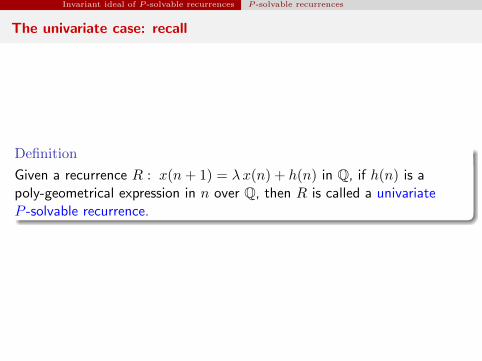
The univariate case: recall
Definition
Given a recurrence R : x(n+ 1) = λx(n) + h(n) in Q, if h(n) is apoly-geometrical expression in n over Q, then R is called a univariateP -solvable recurrence.
Invariant ideal of P -solvable recurrences P -solvable recurrences
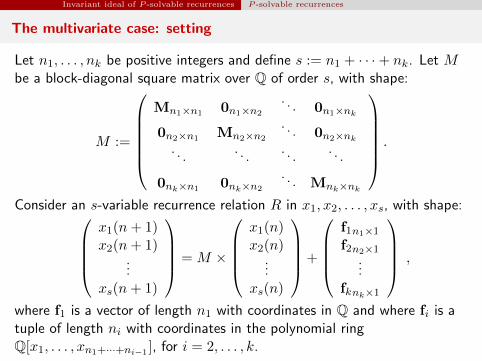
The multivariate case: setting
Let n1, . . . , nk be positive integers and define s := n1 + · · ·+ nk. Let Mbe a block-diagonal square matrix over Q of order s, with shape:
M :=
Mn1×n1 0n1×n2
. . . 0n1×nk
0n2×n1 Mn2×n2
. . . 0n2×nk
. . .. . .
. . .. . .
0nk×n1 0nk×n2
. . . Mnk×nk
.
Consider an s-variable recurrence relation R in x1, x2, . . . , xs, with shape:x1(n+ 1)x2(n+ 1)
...xs(n+ 1)
= M ×
x1(n)x2(n)
...xs(n)
+
f1n1×1f2n2×1
...fknk×1
,
where f1 is a vector of length n1 with coordinates in Q and where fi is atuple of length ni with coordinates in the polynomial ringQ[x1, . . . , xn1+···+ni−1 ], for i = 2, . . . , k.
Invariant ideal of P -solvable recurrences P -solvable recurrences
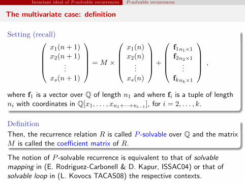
The multivariate case: definition
Setting (recall)x1(n+ 1)x2(n+ 1)
...xs(n+ 1)
= M ×
x1(n)x2(n)
...xs(n)
+
f1n1×1f2n2×1
...fknk×1
,
where f1 is a vector over Q of length n1 and where fi is a tuple of lengthni with coordinates in Q[x1, . . . , xn1+···+ni−1 ], for i = 2, . . . , k.
Definition
Then, the recurrence relation R is called P -solvable over Q and the matrixM is called the coefficient matrix of R.
The notion of P -solvable recurrence is equivalent to that of solvablemapping in (E. Rodriguez-Carbonell & D. Kapur, ISSAC04) or that ofsolvable loop in (L. Kovocs TACAS08) the respective contexts.
Invariant ideal of P -solvable recurrencesDegree estimates for solutions of P -solvable
recurrences
Plan
1 PreliminariesNotions on loop invariantsPoly-geometric summationsA variation on Bezout’s Theorem
2 Invariant ideal of P -solvable recurrencesDegree estimates for solutions of P -solvable recurrencesP -solvable recurrencesDegree estimates for solutions of P -solvable recurrencesDegree estimates for their invariant idealDimension estimates for their invariant ideal
3 Loop invariant generation via polynomial interpolationA direct approachA modular methodExperimentationMaple Package: ProgramAnalysis
Invariant ideal of P -solvable recurrencesDegree estimates for solutions of P -solvable
recurrences
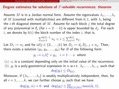
Degree estimates for solutions of P -solvable recurrences: theorem
Assume M is in a Jordan normal form. Assume the eigenvalues λ1, . . . , λsof M (counted with multiplicities) are different from 0, 1, with λi beingthe i-th diagonal element of M . Assume for each block j the total degreeof any polynomial in fj (for i = 2 · · · k) is upper bounded by dj . For eachi, we denote by b(i) the block number of the index i, that is,∑b(i)−1
j=1 nj < i ≤∑b(i)
j=1 nj .
Let D1 := n1 and for allj ∈ {2, . . . , k} let Dj := dj Dj−1 + nj . Then,there exists a solution (y1, y2, . . . , ys) for R of the following form:
yi := ciλni + gi, i = 1 · · · s where
(a) ci is a constant depending only on the initial value of the recurrence;(b) gi is a poly-geometrical expression in n w.r.t. λ1, . . . , λi−1, such that
deg(gi) ≤ Db(i).
Moreover, if {λ1, . . . , λs} is weakly multiplicatively independent, then, forall i = 1, . . . , k, we can further choose yi such that we have
deg(gi, n) = 0 and deg(gi) ≤∏
2≤t≤b(i) max(dt, 1).
Invariant ideal of P -solvable recurrencesDegree estimates for solutions of P -solvable
recurrences
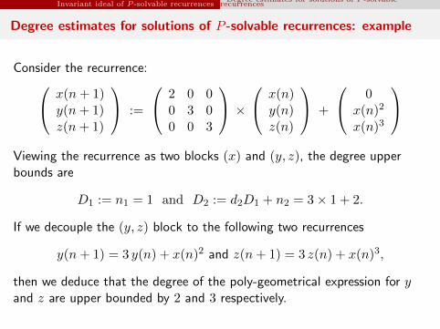
Degree estimates for solutions of P -solvable recurrences: example
Consider the recurrence: x(n+ 1)y(n+ 1)z(n+ 1)
:=
2 0 00 3 00 0 3
× x(n)
y(n)z(n)
+
0x(n)2
x(n)3
Viewing the recurrence as two blocks (x) and (y, z), the degree upperbounds are
D1 := n1 = 1 and D2 := d2D1 + n2 = 3× 1 + 2.
If we decouple the (y, z) block to the following two recurrences
y(n+ 1) = 3 y(n) + x(n)2 and z(n+ 1) = 3 z(n) + x(n)3,
then we deduce that the degree of the poly-geometrical expression for yand z are upper bounded by 2 and 3 respectively.
Invariant ideal of P -solvable recurrencesDegree estimates for solutions of P -solvable
recurrences
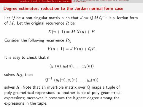
Degree estimates: reduction to the Jordan normal form case
Let Q be a non-singular matrix such that J := QM Q−1 is a Jordan formof M . Let the original recurrence R be
X(n+ 1) = M X(n) + F.
Consider the following recurrence RQ
Y (n+ 1) = J Y (n) +QF.
It is easy to check that if
(y1(n), y2(n), . . . , ys(n))
solves RQ, thenQ−1 (y1(n), y2(n), . . . , ys(n))
solves R. Note that an invertible matrix over Q maps a tuple ofpoly-geometrical expressions to another tuple of poly-geometricalexpressions; moreover it preserves the highest degree among theexpressions in the tuple.
Invariant ideal of P -solvable recurrences Degree estimates for their invariant ideal
Plan
1 PreliminariesNotions on loop invariantsPoly-geometric summationsA variation on Bezout’s Theorem
2 Invariant ideal of P -solvable recurrencesDegree estimates for solutions of P -solvable recurrencesP -solvable recurrencesDegree estimates for solutions of P -solvable recurrencesDegree estimates for their invariant idealDimension estimates for their invariant ideal
3 Loop invariant generation via polynomial interpolationA direct approachA modular methodExperimentationMaple Package: ProgramAnalysis
Invariant ideal of P -solvable recurrences Degree estimates for their invariant ideal
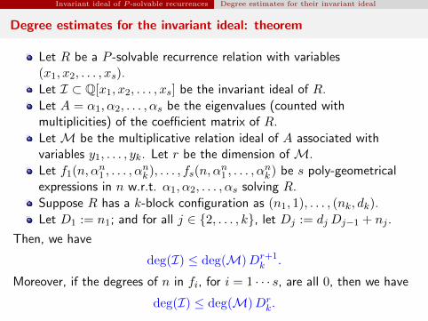
Degree estimates for the invariant ideal: theorem
Let R be a P -solvable recurrence relation with variables(x1, x2, . . . , xs).
Let I ⊂ Q[x1, x2, . . . , xs] be the invariant ideal of R.
Let A = α1, α2, . . . , αs be the eigenvalues (counted withmultiplicities) of the coefficient matrix of R.
Let M be the multiplicative relation ideal of A associated withvariables y1, . . . , yk. Let r be the dimension of M.
Let f1(n, αn1 , . . . , α
nk), . . . , fs(n, α
n1 , . . . , α
nk) be s poly-geometrical
expressions in n w.r.t. α1, α2, . . . , αs solving R.
Suppose R has a k-block configuration as (n1, 1), . . . , (nk, dk).
Let D1 := n1; and for all j ∈ {2, . . . , k}, let Dj := dj Dj−1 + nj .
Then, we have
deg(I) ≤ deg(M)Dr+1k .
Moreover, if the degrees of n in fi, for i = 1 · · · s, are all 0, then we have
deg(I) ≤ deg(M)Drk.
Invariant ideal of P -solvable recurrences Degree estimates for their invariant ideal
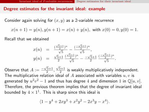
Degree estimates for the invariant ideal: example
Consider again solving for (x, y) as a 2-variable recurrence
x(n+ 1) = y(n), y(n+ 1) = x(n) + y(n), with x(0) = 0, y(0) = 1.
Recall that we obtained
x(n) =(√5+12
)n√5− (−
√5+12
)n√5
,
y(n) =√5+12
(√5+12
)n√5− −
√5+12
(−√5+12
)n√5
.
Observe that A := −√5+12 ,
√5+12 is weakly multiplicatively independent.
The multiplicative relation ideal of A associated with variables u, v isgenerated by u2v2 − 1 and thus has degree 4 and dimension 1 in Q[u, v].Therefore, the previous theorem implies that the degree of invariant idealbounded by 4× 11. This is sharp since this ideal is
〈1− y4 + 2xy3 + x2y2 − 2x3y − x4〉.
Invariant ideal of P -solvable recurrences Dimension estimates for their invariant ideal
Plan
1 PreliminariesNotions on loop invariantsPoly-geometric summationsA variation on Bezout’s Theorem
2 Invariant ideal of P -solvable recurrencesDegree estimates for solutions of P -solvable recurrencesP -solvable recurrencesDegree estimates for solutions of P -solvable recurrencesDegree estimates for their invariant idealDimension estimates for their invariant ideal
3 Loop invariant generation via polynomial interpolationA direct approachA modular methodExperimentationMaple Package: ProgramAnalysis
Invariant ideal of P -solvable recurrences Dimension estimates for their invariant ideal
Dimension estimates for the invariant ideal: theorem
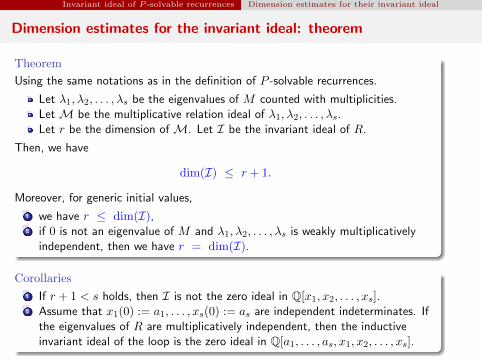
Theorem
Using the same notations as in the definition of P -solvable recurrences.
Let λ1, λ2, . . . , λs be the eigenvalues of M counted with multiplicities.Let M be the multiplicative relation ideal of λ1, λ2, . . . , λs.Let r be the dimension of M. Let I be the invariant ideal of R.
Then, we have
dim(I) ≤ r + 1.
Moreover, for generic initial values,
1 we have r ≤ dim(I),2 if 0 is not an eigenvalue of M and λ1, λ2, . . . , λs is weakly multiplicatively
independent, then we have r = dim(I).
Corollaries
1 If r + 1 < s holds, then I is not the zero ideal in Q[x1, x2, . . . , xs].2 Assume that x1(0) := a1, . . . , xs(0) := as are independent indeterminates. If
the eigenvalues of R are multiplicatively independent, then the inductiveinvariant ideal of the loop is the zero ideal in Q[a1, . . . , as, x1, x2, . . . , xs].
Invariant ideal of P -solvable recurrences Dimension estimates for their invariant ideal
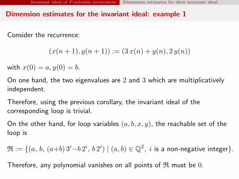
Dimension estimates for the invariant ideal: example 1
Consider the recurrence:
(x(n+ 1), y(n+ 1)) := (3x(n) + y(n), 2 y(n))
with x(0) = a, y(0) = b.
On one hand, the two eigenvalues are 2 and 3 which are multiplicativelyindependent.
Therefore, using the previous corollary, the invariant ideal of thecorresponding loop is trivial.
On the other hand, for loop variables (a, b, x, y), the reachable set of theloop is
R := {(a, b, (a+b) 3i−b 2i, b 2i) | (a, b) ∈ Q2, i is a non-negative integer}.
Therefore, any polynomial vanishes on all points of R must be 0.
Invariant ideal of P -solvable recurrences Dimension estimates for their invariant ideal
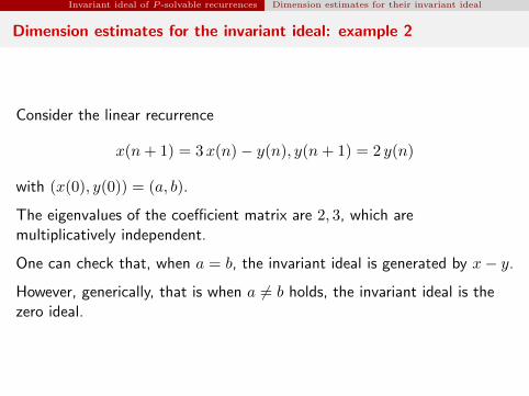
Dimension estimates for the invariant ideal: example 2
Consider the linear recurrence
x(n+ 1) = 3x(n)− y(n), y(n+ 1) = 2 y(n)
with (x(0), y(0)) = (a, b).
The eigenvalues of the coefficient matrix are 2, 3, which aremultiplicatively independent.
One can check that, when a = b, the invariant ideal is generated by x− y.
However, generically, that is when a 6= b holds, the invariant ideal is thezero ideal.

Loop invariant generation via polynomial interpolation A direct approach
Plan
1 PreliminariesNotions on loop invariantsPoly-geometric summationsA variation on Bezout’s Theorem
2 Invariant ideal of P -solvable recurrencesDegree estimates for solutions of P -solvable recurrencesP -solvable recurrencesDegree estimates for solutions of P -solvable recurrencesDegree estimates for their invariant idealDimension estimates for their invariant ideal
3 Loop invariant generation via polynomial interpolationA direct approachA modular methodExperimentationMaple Package: ProgramAnalysis
Loop invariant generation via polynomial interpolation A direct approach
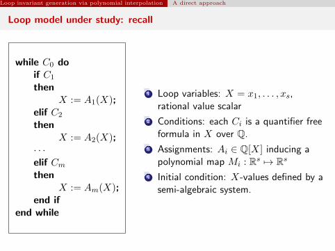
Loop model under study: recall
while C0 doif C1
thenX := A1(X);
elif C2
thenX := A2(X);
· · ·elif Cmthen
X := Am(X);end if
end while
1 Loop variables: X = x1, . . . , xs,rational value scalar
2 Conditions: each Ci is a quantifier freeformula in X over Q.
3 Assignments: Ai ∈ Q[X] inducing apolynomial map Mi : Rs 7→ Rs
4 Initial condition: X-values defined by asemi-algebraic system.
Loop invariant generation via polynomial interpolation A direct approach
A direct approach
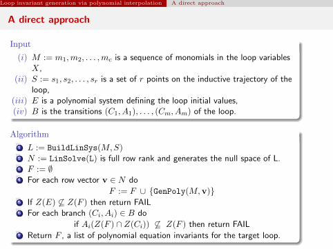
Input
(i) M := m1,m2, . . . ,mc is a sequence of monomials in the loop variablesX,
(ii) S := s1, s2, . . . , sr is a set of r points on the inductive trajectory of theloop,
(iii) E is a polynomial system defining the loop initial values,(iv) B is the transitions (C1, A1), . . . , (Cm, Am) of the loop.
Algorithm
1 L := BuildLinSys(M,S)2 N := LinSolve(L) is full row rank and generates the null space of L.3 F := ∅4 For each row vector v ∈ N do
F := F ∪ {GenPoly(M,v)}5 If Z(E) 6⊆ Z(F ) then return FAIL6 For each branch (Ci, Ai) ∈ B do
if Ai(Z(F ) ∩ Z(Ci)) 6⊆ Z(F ) then return FAIL7 Return F , a list of polynomial equation invariants for the target loop.

Loop invariant generation via polynomial interpolation A modular method
Plan
1 PreliminariesNotions on loop invariantsPoly-geometric summationsA variation on Bezout’s Theorem
2 Invariant ideal of P -solvable recurrencesDegree estimates for solutions of P -solvable recurrencesP -solvable recurrencesDegree estimates for solutions of P -solvable recurrencesDegree estimates for their invariant idealDimension estimates for their invariant ideal
3 Loop invariant generation via polynomial interpolationA direct approachA modular methodExperimentationMaple Package: ProgramAnalysis
Loop invariant generation via polynomial interpolation A modular method
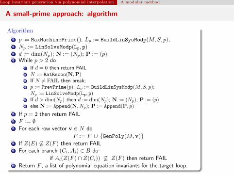
A small-prime approach: algorithm
Algorithm
1 p := MaxMachinePrime(); Lp := BuildLinSysModp(M,S, p);2 Np := LinSolveModp(Lp, p)3 d := dim(Np); N := (Np); P := (p);4 While p > 2 do
1 If d = 0 then return FAIL2 N := RatRecon(N,P)3 If N 6= FAIL then break;4 p := PrevPrime(p); Lp := BuildLinSysModp(M,S, p);Np := LinSolveModp(Lp, p)
5 If d > dim(Np) then d := dim(Np); N := (Np); P := (p)6 else N := Append(N, Np); P := Append(P, p)
5 If p = 2 then return FAIL6 F := ∅7 For each row vector v ∈ N do
F := F ∪ {GenPoly(M,v)}8 If Z(E) 6⊆ Z(F ) then return FAIL9 For each branch (Ci, Ai) ∈ B do
if Ai(Z(F ) ∩ Z(Ci)) 6⊆ Z(F ) then return FAIL10 Return F , a list of polynomial equation invariants for the target loop.
Loop invariant generation via polynomial interpolation A modular method
A small-prime approach: complexity result
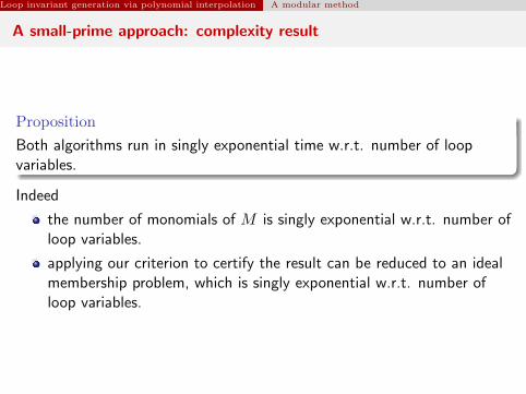
Proposition
Both algorithms run in singly exponential time w.r.t. number of loopvariables.
Indeed
the number of monomials of M is singly exponential w.r.t. number ofloop variables.
applying our criterion to certify the result can be reduced to an idealmembership problem, which is singly exponential w.r.t. number ofloop variables.
Loop invariant generation via polynomial interpolation A modular method
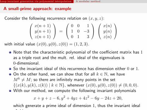
A small-prime approach: example
Consider the following recurrence relation on (x, y, z): x(n+ 1)y(n+ 1)z(n+ 1)
=
0 0 11 0 −30 1 3
x(n)y(n)z(n)
with initial value (x(0), y(0), z(0)) = (1, 2, 3).
Note that the characteristic polynomial of the coefficient matrix has 1as a triple root and the mult. rel. ideal of the eigenvalues is0-dimensional.So the invariant ideal of this recurrence has dimension either 0 or 1.On the other hand, we can show that for all k ∈ N, we haveMk 6= M ; so there are infinitely many points in the set{(x(k), y(k), z(k)) | k ∈ N}, whenever (x(0), y(0), z(0)) 6= (0, 0, 0).With our method, we compute the following invariant polynomials
x+ y + z − 6, y2 + 4yz + 4z2 − 6y − 24z + 20,
which generate a prime ideal of dimension 1, thus the invariant idealof this recurrence.

Loop invariant generation via polynomial interpolation Experimentation
Plan
1 PreliminariesNotions on loop invariantsPoly-geometric summationsA variation on Bezout’s Theorem
2 Invariant ideal of P -solvable recurrencesDegree estimates for solutions of P -solvable recurrencesP -solvable recurrencesDegree estimates for solutions of P -solvable recurrencesDegree estimates for their invariant idealDimension estimates for their invariant ideal
3 Loop invariant generation via polynomial interpolationA direct approachA modular methodExperimentationMaple Package: ProgramAnalysis
Loop invariant generation via polynomial interpolation Experimentation
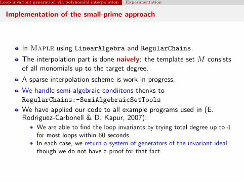
Implementation of the small-prime approach
In Maple using LinearAlgebra and RegularChains.
The interpolation part is done naively: the template set M consistsof all monomials up to the target degree.
A sparse interpolation scheme is work in progress.
We handle semi-algebraic condiitons thenks toRegularChains:-SemiAlgebraicSetTools
We have applied our code to all example programs used in (E.Rodriguez-Carbonell & D. Kapur, 2007):
• We are able to find the loop invariants by trying total degree up to 4for most loops within 60 seconds.
• In each case, we return a system of generators of the invariant ideal,though we do not have a proof for that fact.
Loop invariant generation via polynomial interpolation Experimentation
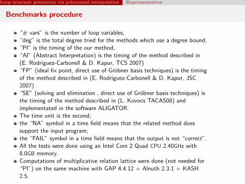
Benchmarks procedure
“# vars” is the number of loop variables,“deg” is the total degree tried for the methods which use a degree bound,“PI” is the timing of the our method,“AI” (Abstract Interpretation) is the timing of the method described in(E. Rodriguez-Carbonell & D. Kapur, TCS 2007)“FP” (ideal fix point, direct use of Grobner basis techniques) is the timingof the method described in (E. Rodriguez-Carbonell & D. Kapur, JSC2007)“SE” (solving and elimination , direct use of Grobner basis techniques) isthe timing of the method described in (L. Kovocs TACAS08) andimplementated in the software ALIGATOR.The time unit is the second;the “NA” symbol in a time field means that the related method doessupport the input program;the “FAIL” symbol in a time field means that the output is not “correct”.All the tests were done using an Intel Core 2 Quad CPU 2.40GHz with8.0GB memory.Computations of multiplicative relation lattice were done (not needed for“PI”) on the same machine with GAP 4.4.12 + Alnuth 2.3.1 + KASH2.5.
Loop invariant generation via polynomial interpolation Experimentation
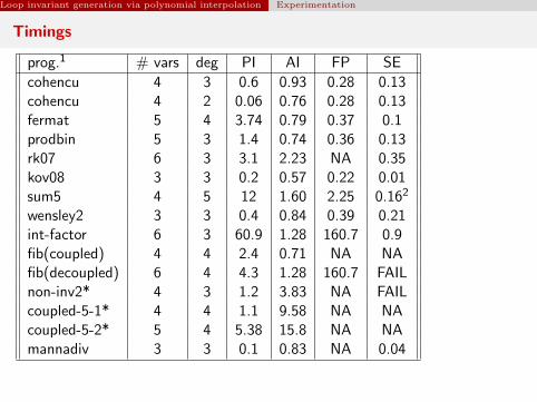
Timings
prog.1 # vars deg PI AI FP SE
cohencu 4 3 0.6 0.93 0.28 0.13cohencu 4 2 0.06 0.76 0.28 0.13fermat 5 4 3.74 0.79 0.37 0.1prodbin 5 3 1.4 0.74 0.36 0.13rk07 6 3 3.1 2.23 NA 0.35kov08 3 3 0.2 0.57 0.22 0.01sum5 4 5 12 1.60 2.25 0.162
wensley2 3 3 0.4 0.84 0.39 0.21int-factor 6 3 60.9 1.28 160.7 0.9fib(coupled) 4 4 2.4 0.71 NA NAfib(decoupled) 6 4 4.3 1.28 160.7 FAILnon-inv2* 4 3 1.2 3.83 NA FAILcoupled-5-1* 4 4 1.1 9.58 NA NAcoupled-5-2* 5 4 5.38 15.8 NA NAmannadiv 3 3 0.1 0.83 NA 0.04

Loop invariant generation via polynomial interpolation Maple Package: ProgramAnalysis
Plan
1 PreliminariesNotions on loop invariantsPoly-geometric summationsA variation on Bezout’s Theorem
2 Invariant ideal of P -solvable recurrencesDegree estimates for solutions of P -solvable recurrencesP -solvable recurrencesDegree estimates for solutions of P -solvable recurrencesDegree estimates for their invariant idealDimension estimates for their invariant ideal
3 Loop invariant generation via polynomial interpolationA direct approachA modular methodExperimentationMaple Package: ProgramAnalysis
Loop invariant generation via polynomial interpolation Maple Package: ProgramAnalysis
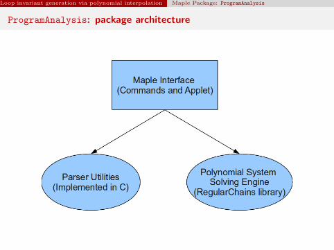
ProgramAnalysis: package architecture
Loop invariant generation via polynomial interpolation Maple Package: ProgramAnalysis
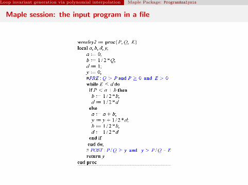
Maple session: the input program in a file
Loop invariant generation via polynomial interpolation Maple Package: ProgramAnalysis
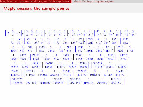
Maple session: the sample points
Loop invariant generation via polynomial interpolation Maple Package: ProgramAnalysis
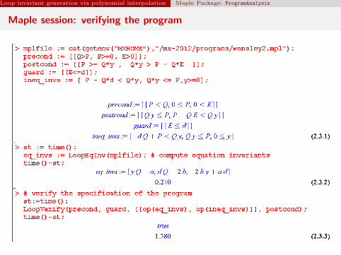
Maple session: verifying the program

Loop invariant generation via polynomial interpolation Maple Package: ProgramAnalysis
Xie Xie!