Generalization of Lambert’s Reflectance Model

Michael Oren and Shree K. NayarDepartment of Computer Science, Columbia University

New York, NY 10027

Abstract

Lambert’s model for body reflection is widely used in computergraphics. It is used extensively by rendering techniques such asradiosity and ray tracing. For several real-world objects, however,Lambert’s model can prove to be a very inaccurate approximationto the body reflectance. While the brightness of a Lambertian sur-face is independent of viewing direction, that of a rough surfaceincreases as the viewing direction approaches the light source di-rection. In this paper, a comprehensive model is developed thatpredicts body reflectance from rough surfaces. The surface is mod-eled as a collection of Lambertian facets. It is shown that such asurface is inherently non-Lambertian due to the foreshortening ofthe surface facets. Further, the model accounts for complex geo-metric and radiometric phenomena such as masking, shadowing,and interreflections between facets. Several experiments have beenconducted on samples of rough diffuse surfaces, such as, plaster,sand, clay, and cloth. All these surfaces demonstrate significant de-viation from Lambertian behavior. The reflectance measurementsobtained are in strong agreement with the reflectance predicted bythe model.

CR Descriptors: I.3.7 [Computer Graphics]: Three-Dimensional Graphics and Realism; I.3.3 [Computer Graphics]:Picture/Image Generation; J.2 [Physical Sciences and Engineer-ing]: Physics.

Additional Key Words: reflection models, Lambert’s model,BRDF, rough surfaces, moon reflectance.

1 Introduction

An active area of research in computer graphics involves the cre-ation of realistic images. Images are rendered using one of twowell-known techniques, namely, ray tracing [36] or radiosity [7].The quality of a rendered image depends to a great extent on theaccuracy of the reflectance model used. In the past decade, com-puter graphics has witnessed the application of several physically-based reflectance models for image rendering (see [8], [17], [10],[14]). Reflection from a surface can be broadly classified intotwo categories: surface reflectance which takes place at the inter-face between two media with different refractive indices and bodyreflectance which is due to subsurface scattering. Most of the pre-vious work on physically-based rendering has focused on accuratemodeling of surface reflectance. They predict ideal specular reflec-

tion from smooth surfaces as well as wide directional lobes fromrougher surfaces [14]. In contrast, the body component has mostoften been assumed to be Lambertian. A Lambertian surface ap-pears equally bright from all directions. This model was advancedby Lambert [20] more than 200 years ago and remains one of themost widely used models in computer graphics.

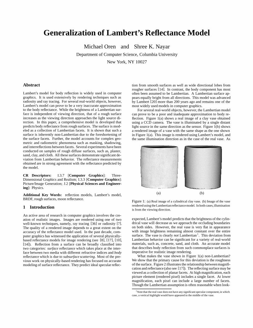
For several real-world objects, however, the Lambertian modelcan prove to be a poor and inadequate approximation to body re-flection. Figure 1(a) shows a real image of a clay vase obtainedusing a CCD camera. The vase is illuminated by a single distantlight source in the same direction as the sensor. Figure 1(b) showsa rendered image of a vase with the same shape as the one shownin Figure 1(a). This image is rendered using Lambert’s model, andthe same illumination direction as in the case of the real vase. As

(a) (b)

Figure 1: (a) Real image of a cylindrical clay vase. (b) Image of the vaserendered using theLambertian reflectancemodel. In both cases,illuminationis from the viewing direction.

expected, Lambert’s model predicts that the brightness of the cylin-drical vase will decrease as we approach the occluding boundarieson both sides. However, the real vase is very flat in appearancewith image brightness remaining almost constant over the entiresurface. The vase is clearly not Lambertian 1. This deviation fromLambertian behavior can be significant for a variety of real-worldmaterials, such as, concrete, sand, and cloth. An accurate modelthat describes body reflection from such commonplace surfaces isimperative for realistic image rendering.

What makes the vase shown in Figure 1(a) non-Lambertian?We show that the primary cause for this deviation is the roughnessof the surface. Figure 2 illustrates the relationship between magnifi-cation and reflectance (also see [17]). The reflecting surface may beviewed as a collection of planar facets. At high magnification, eachpicture element (rendered pixel) includes a single facet. At lowermagnification, each pixel can include a large number of facets.Though the Lambertian assumption is often reasonable when look-

1Note that the real vase does not have any significant specular component, in whichcase, a vertical highlight would have appeared in the middle of the vase.

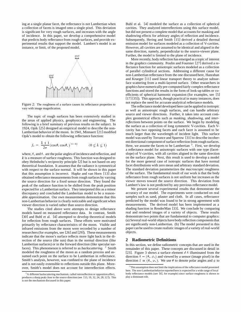
ing at a single planar facet, the reflectance is not Lambertian whena collection of facets is imaged onto a single pixel. This deviationis significant for very rough surfaces, and increases with the angleof incidence. In this paper, we develop a comprehensive modelthat predicts body reflectance from rough surfaces, and provide ex-perimental results that support the model. Lambert’s model is aninstance, or limit, of the proposed model.

pixel

pixel

Figure 2: The roughness of a surface causes its reflectance properties tovary with image magnification.

The topic of rough surfaces has been extensively studied inthe areas of applied physics, geophysics and engineering. Thefollowing is a brief summary of previous results on the subject. In1924, Opik [25] designed an empirical model to describe the non-Lambertian behavior of the moon. In 1941, Minnaert [21] modifiedOpik’s model to obtain the following reflectance function:

fr �k� 1

2��cos�i cos�r�

�k�1� �0 � k � 1�

where, �i and�r are the polar angles of incidence and reflection, andk is a measure of surface roughness. This function was designed toobey Helmholtz’s reciprocity principle [2] but is not based on anytheoretical foundation. It assumes that the radiance is symmetricalwith respect to the surface normal. It will be shown in this paperthat this assumption is incorrect. Hapke and van Horn [13] alsoobtained reflectance measurements from rough surfaces by varyingthe source direction for a fixed sensor direction. They found thepeak of the radiance function to be shifted from the peak positionexpected for a Lambertian surface. They interpreted this as a minordiscrepancy and concluded the Lambertian model to be a reason-able approximation. Our own measurements demonstrate that thisnon-Lambertian behavior is clearly noticeable and significant whenviewer direction is varied rather than source direction.

The studies cited above were attempts to design reflectancemodels based on measured reflectance data. In contrast, Smith[30] and Buhl et al. [4] attempted to develop theoretical modelsfor reflection from rough surfaces. These efforts were motivatedprimarily by reflectance characteristics of the moon. Visible andinfrared emissions from the moon were recorded by a number ofresearchers (for examples, see [26] and [29]). These measurementsindicate that the moon’s surface reflects more light back in the di-rection of the source (the sun) than in the normal direction (likeLambertian surfaces) or in the forward direction (like specular sur-faces). This phenomenon is referred to as backscattering. 2 Smithmodeled the roughness of the moon as a random process and as-sumed each point on the surface to be Lambertian in reflectance.Smith’s analysis, however, was confined to the plane of incidenceand is not easily extensible to reflections outside this plane. More-over, Smith’s model does not account for interreflection effects.

2A different backscattering mechanism, called retroreflection or opposition effect,produces a sharp peak close to the source direction (see [13, 19, 32, 24, 28, 12 ]). Thisis not the mechanism discussed in this paper.

Buhl et al. [4] modeled the surface as a collection of sphericalcavities. They analyzed interreflections using this surface model,but did not present a complete model that accounts for masking andshadowing effects for arbitrary angles of reflection and incidence.Subsequently, Hering and Smith [15] derived a detailed thermalemission model for surfaces modeled as a collection of V-cavities.However, all cavities are assumed to be identical and aligned in thesame direction, namely, perpendicular to the source-viewer plane.Further, the model is limited to the plane of incidence.

More recently, body reflection has emerged as a topic of interestin the graphics community. Poulin and Fournier [27] derived a re-flectance function for anisotropic surfaces modeled as a collectionof parallel cylindrical sections. Addressing a different cause fornon-Lambertian reflectance from the one discussed here, Hanrahanand Krueger [11] used linear transport theory to analyze subsur-face scattering from a multi-layered surface. Other researchers ingraphics have numerically pre-computed fairly complex reflectancefunctions and stored the results in the form of look-up tables or co-efficients of spherical harmonic expansion (for examples, see [5][17] [35]). This approach, though practical in many instances, doesnot replace the need for accurate analytical reflectance models.

The reflectance model developed here can be applied to isotropicas well as anisotropic rough surfaces, and can handle arbitrarysource and viewer directions. Further, it takes into account com-plex geometrical effects such as masking, shadowing, and inter-reflections between points on the surface. We begin by modelingthe surface as a collection of long symmetric V-cavities. Each V-cavity has two opposing facets and each facet is assumed to bemuch larger than the wavelength of incident light. This surfacemodel was used by Torrance and Sparrow [31] to describe incoher-ent directional component of surface reflection from rough surfaces.Here, we assume the facets to be Lambertian 3. First, we developa reflectance model for anisotropic surfaces with one type (facet-slope) of V-cavities, with all cavities aligned in the same directionon the surface plane. Next, this result is used to develop a modelfor the more general case of isotropic surfaces that have normalfacet distributions with zero mean and arbitrary standard deviation.The standard deviation parameterizes the macroscopic roughnessof the surface. The fundamental result of our work is that the bodyreflectance from rough surfaces is not uniform but increases as theviewer moves toward the source direction. This deviation fromLambert’s law is not predicted by any previous reflectance model.

We present several experimental results that demonstrate theaccuracy of our model. The experiments were conducted on realsamples such as sand, plaster and cloth. In all cases, reflectancepredicted by the model was found to be in strong agreement withmeasurements. The derived model has been implemented as ashading function in RenderMan [33]. We conclude by comparingreal and rendered images of a variety of objects. These resultsdemonstrate two points that are fundamental to computer graphics:(a) Several real-world objects have body reflection components thatare significantly non-Lambertian. (b) The model presented in thispaper can be used to create realistic images of a variety of real-worldobjects.

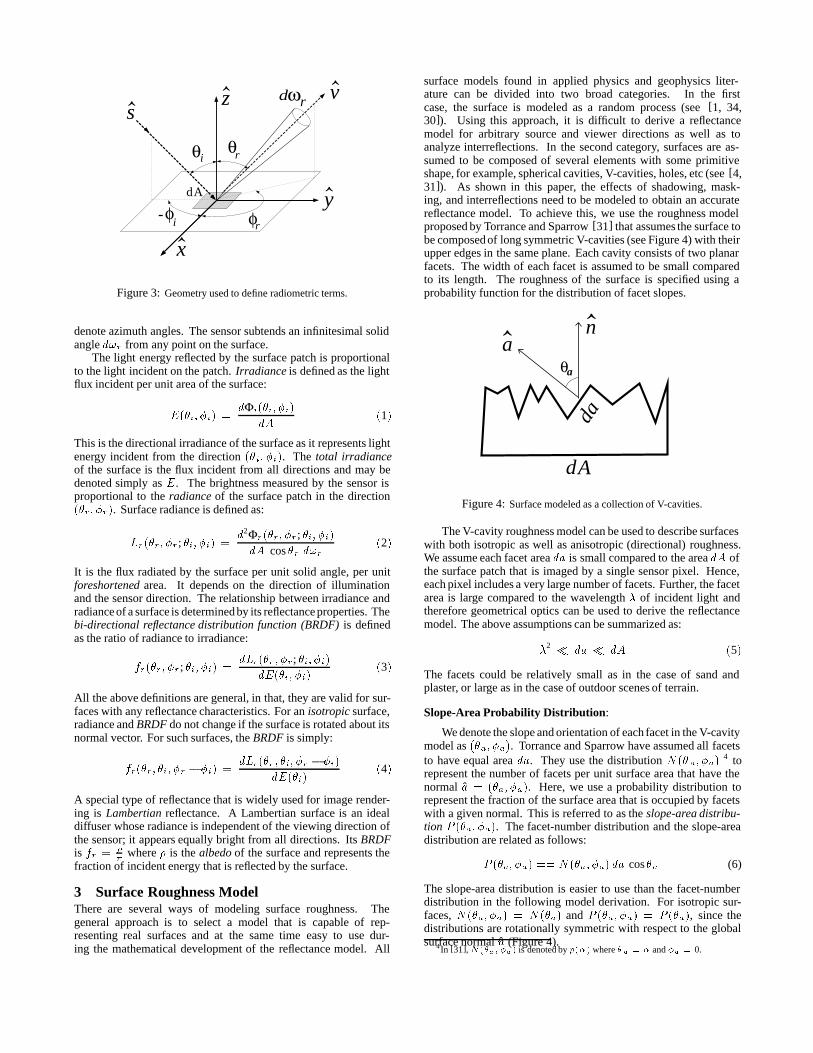
2 Radiometric DefinitionsIn this section, we define radiometric concepts that are used in theremainder of this paper. These concepts are discussed in detail in[23]. Figure 3 shows a surface element dA illuminated from thedirection s � ��i� �i� and viewed by a sensor (image pixel) in thedirection v � ��r� �r�. We use � to denote polar angles and � to

3This assumption does not limit the implications of the reflectance model presentedhere. The non-Lambertianbehavior reported here is expected for a wide range of localbody reflectance models (see [6], for example) since surface roughness is shown toplay a dominant role.

s

θi

φrφ

i-

z

x

dωr

rθ

v

ydA

Figure 3: Geometry used to define radiometric terms.

denote azimuth angles. The sensor subtends an infinitesimal solidangle d�r from any point on the surface.

The light energy reflected by the surface patch is proportionalto the light incident on the patch. Irradiance is defined as the lightflux incident per unit area of the surface:

E��i� �i� �dΦi��i� �i�

dA�1�

This is the directional irradiance of the surface as it represents lightenergy incident from the direction ��i� �i�. The total irradianceof the surface is the flux incident from all directions and may bedenoted simply as E. The brightness measured by the sensor isproportional to the radiance of the surface patch in the direction��r� �r�. Surface radiance is defined as:

Lr��r� �r; �i� �i� �d2Φr��r� �r; �i� �i�dA cos �r d�r

�2�

It is the flux radiated by the surface per unit solid angle, per unitforeshortened area. It depends on the direction of illuminationand the sensor direction. The relationship between irradiance andradiance of a surface is determined by its reflectance properties. Thebi-directional reflectance distribution function (BRDF) is definedas the ratio of radiance to irradiance:

fr��r� �r; �i� �i� �dLr��r � �r; �i� �i�

dE��i� �i��3�

All the above definitions are general, in that, they are valid for sur-faces with any reflectance characteristics. For an isotropic surface,radiance and BRDF do not change if the surface is rotated about itsnormal vector. For such surfaces, the BRDF is simply:

fr��r� �i� �r � �i� �dLr��r � �i� �r � �i�

dE��i��4�

A special type of reflectance that is widely used for image render-ing is Lambertian reflectance. A Lambertian surface is an idealdiffuser whose radiance is independent of the viewing direction ofthe sensor; it appears equally bright from all directions. Its BRDFis fr � �

�where � is the albedo of the surface and represents the

fraction of incident energy that is reflected by the surface.

3 Surface Roughness ModelThere are several ways of modeling surface roughness. Thegeneral approach is to select a model that is capable of rep-resenting real surfaces and at the same time easy to use dur-ing the mathematical development of the reflectance model. All

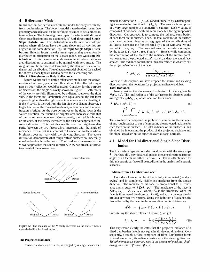
surface models found in applied physics and geophysics liter-ature can be divided into two broad categories. In the firstcase, the surface is modeled as a random process (see [1, 34,30]). Using this approach, it is difficult to derive a reflectancemodel for arbitrary source and viewer directions as well as toanalyze interreflections. In the second category, surfaces are as-sumed to be composed of several elements with some primitiveshape, for example, spherical cavities, V-cavities, holes, etc (see [4,31]). As shown in this paper, the effects of shadowing, mask-ing, and interreflections need to be modeled to obtain an accuratereflectance model. To achieve this, we use the roughness modelproposed by Torrance and Sparrow [31] that assumes the surface tobe composed of long symmetric V-cavities (see Figure 4) with theirupper edges in the same plane. Each cavity consists of two planarfacets. The width of each facet is assumed to be small comparedto its length. The roughness of the surface is specified using aprobability function for the distribution of facet slopes.

d

a

dA

an

θa

^

Figure 4: Surface modeled as a collection of V-cavities.

The V-cavity roughness model can be used to describe surfaceswith both isotropic as well as anisotropic (directional) roughness.We assume each facet area da is small compared to the area dA ofthe surface patch that is imaged by a single sensor pixel. Hence,each pixel includes a very large number of facets. Further, the facetarea is large compared to the wavelength � of incident light andtherefore geometrical optics can be used to derive the reflectancemodel. The above assumptions can be summarized as:

�2 � da � dA �5�

The facets could be relatively small as in the case of sand andplaster, or large as in the case of outdoor scenes of terrain.

Slope-Area Probability Distribution:

We denote the slope and orientation of each facet in the V-cavitymodel as ��a� �a�. Torrance and Sparrow have assumed all facetsto have equal area da. They use the distribution N�� a� �a�

4 torepresent the number of facets per unit surface area that have thenormal a � ��a� �a�. Here, we use a probability distribution torepresent the fraction of the surface area that is occupied by facetswith a given normal. This is referred to as the slope-area distribu-tion P ��a� �a�. The facet-number distribution and the slope-areadistribution are related as follows:

P ��a� �a� �� N��a� �a� da cos�a (6)

The slope-area distribution is easier to use than the facet-numberdistribution in the following model derivation. For isotropic sur-faces, N��a� �a� � N��a� and P ��a� �a� � P ��a�, since thedistributions are rotationally symmetric with respect to the globalsurface normal n (Figure 4).4In [31], N��a � �a� is denoted by p��� where �a � � and�a � 0.

4 Reflectance ModelIn this section, we derive a reflectance model for body reflectancefrom rough surfaces. The V-cavity model is used to describe surfacegeometry and each facet on the surface is assumed to be Lambertianin reflectance. The following three types of surfaces with differentslope-area distributions are examined. (a) Uni-directional Single-Slope Distribution: This distribution results in a non-isotropicsurface where all facets have the same slope and all cavities arealigned in the same direction. (b) Isotropic Single-Slope Distri-bution: Here, all facets have the same slope but they are uniformlydistributed in orientation on the surface plane. (c) Gaussian Dis-tribution: This is the most general case examined where the slope-area distribution is assumed to be normal with zero mean. Theroughness of the surface is determined by the standard deviation ofthe normal distribution. The reflectance model obtained for each ofthe above surface types is used to derive the succeeding one.Effect of Roughness on Body Reflectance:

Before we proceed to derive reflectance models for the above-mentioned surface types, a brief illustration of the effect of rough-ness on body reflection would be useful. Consider, for the purposeof discussion, the single V-cavity shown in Figure 5. Both facetsof the cavity are fully illuminated by a distant source on the rightside. If the facets are Lambertian with equal albedo, the left facetappears brighter than the right one as it receives more incident light.If the V-cavity is viewed from the left side by a distant observer, alarger fraction of the foreshortened cavity area is dark and a smallerfraction is bright. As the observer moves to the right, towards thesource direction, the fraction of brighter area increases while thatof the darker area decreases. Consequently, the total brightness,or radiance, of the cavity increases as the observer approaches thesource direction. Note that this results from the brightness dis-parity between the two facets which increases with the angle ofincidence. This effect is in contrast to Lambertian surfaces whosebrightness does not vary with the viewing direction. The aboveillustration demonstrates that rough diffuse surfaces are inherentlynon-Lambertian in reflectance. Their radiance increases as theviewer approaches the source direction. Now we present a formaltreatment of the above effects.

Brighter Darker

Source direction

Viewer direction Viewer direction

Brighter Darker Brighter Darker

Figure 5: The radiance of the V-cavity increases as the viewer movestowards the illumination direction.

The Projected Radiance:

Consider surface area dA that is imaged by a single sensor ele-

ment in the direction v � ��r � �r� and illuminated by a distant pointlight source in the direction s � ��i� �i�. The area dA is composedof a very large number of symmetric V-cavities. Each V-cavity iscomposed of two facets with the same slope but facing in oppositedirections. Our approach is to compute the radiance contributionof each facet on the surface. Then, the total radiance of the surfacepatch can be determined as an aggregate of the contributions ofall facets. Consider the flux reflected by a facet with area da andnormal a � ��a� �a�. The projected area on the surface occupiedby the facet is da cos�a (see Figure 4). Hence, while computingthe contribution of the facet to the radiance of the surface patch,we need to use the projected area da cos � a and not the actual facetarea da. The radiance contribution thus determined is what we callthe projected radiance of the facet:

Lrp��a� �a� �d2Φr��a� �a�

�da cos�a� cos �r d�r�7�

For ease of description, we have dropped the source and viewingdirections from the notations for projected radiance and flux.Total Radiance:

Now consider the slope-area distribution of facets given byP ��a� �a�. The total radiance of the surface can be obtained as theaverage of Lrp��a� �a� of all facets on the surface:

Lr��r� �r; �i� �i� � (8)Z �2

�a�0

Z 2�

�a�0

P ��a� �a�Lrp��a� �a� sin �a d�a d�a

Thus, we have decomposed the problem of computing the radianceof any rough surface to one of computing the projected radiance foreach facet on the surface. The total radiance of the surface is thenobtained by integrating the product of the projected radiance andthe slope-area distribution function over all facet normals.

4.1 Model for Uni-directional Single-Slope Distri-bution

The first surface type we consider has all facets with the same slope�a. Further, all V-cavities are aligned in the same direction; azimuthangles of all facets are either �a or �a��. The results obtained forthis anisotropic surface will be used later in the analysis of isotropicsurfaces.

Radiance from a Lambertian Facet:

Consider a Lambertian facet that is fully illuminated (no shad-owing) and is completely visible (no masking) from the sensordirection. The radiance of the facet is proportional to its irradi-ance and is equal to �

�E��a� �a�. The irradiance of the facet isE��a� �a� � E0�s� a�, where, E0 is the irradiance when thefacet is illuminated head-on (i.e. s = a), and� � � denotes the dotproduct between two vectors. Using the definition of radiance, theflux reflected by the facet in the sensor direction is obtained as:

d2Φr � ��E0 �s� a��v� a� dad�r �9�

Substituting the above reflected flux in (7), we get:

Lrp��a� �a� ��

�E0

�s� a��v� a�

�a� n��v� n�(10)

This expression clearly indicates that the projected radiance of atilted Lambertian facet is not equal in all viewing directions. Con-sequently, a rough surface comprised of tilted Lambertian facetsis non-Lambertian; its radiance varies with the viewing direction.This phenomenonis observedeven in the absenceof masking, shad-owing, and interreflection effects.

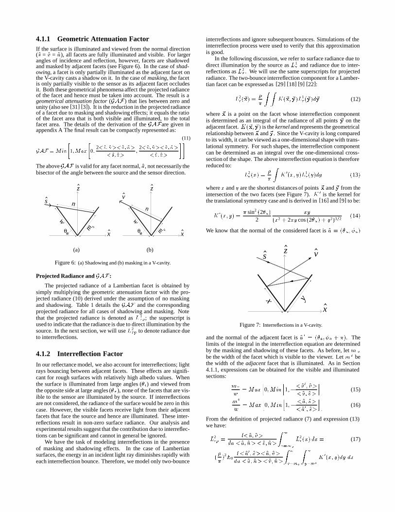
4.1.1 Geometric Attenuation FactorIf the surface is illuminated and viewed from the normal direction(s = v = n), all facets are fully illuminated and visible. For largerangles of incidence and reflection, however, facets are shadowedand masked by adjacent facets (see Figure 6). In the case of shad-owing, a facet is only partially illuminated as the adjacent facet onthe V-cavity casts a shadow on it. In the case of masking, the facetis only partially visible to the sensor as its adjacent facet occludesit. Both these geometrical phenomena affect the projected radianceof the facet and hence must be taken into account. The result is ageometrical attenuation factor (GAF ) that lies between zero andunity (also see [31] [3]). It is the reduction in the projected radianceof a facet due to masking and shadowing effects; it equals the ratioof the facet area that is both visible and illuminated, to the totalfacet area. The details of the derivation of the GAFare given inappendix A The final result can be compactly represented as:

(11)

GAF � Min

�1�Max

�0�

2�s� n��a� n�

�s� a��

2�v� n��a� n�

�v� a�

��The aboveGAF is valid for any facet normal, a, not necessarily thebisector of the angle between the source and the sensor direction.

x

z

n

m s

s

w

^

^

^θa x

z

n

w

^

^θa m v

v ^

(a) (b)

Figure 6: (a) Shadowing and (b) masking in a V-cavity.

Projected Radiance and GAF :

The projected radiance of a Lambertian facet is obtained bysimply multiplying the geometric attenuation factor with the pro-jected radiance (10) derived under the assumption of no maskingand shadowing. Table 1 details the GAF and the correspondingprojected radiance for all cases of shadowing and masking. Notethat the projected radiance is denoted as L 1

rp; the superscript isused to indicate that the radiance is due to direct illumination by thesource. In the next section, we will use L2

rp to denote radiance dueto interreflections.

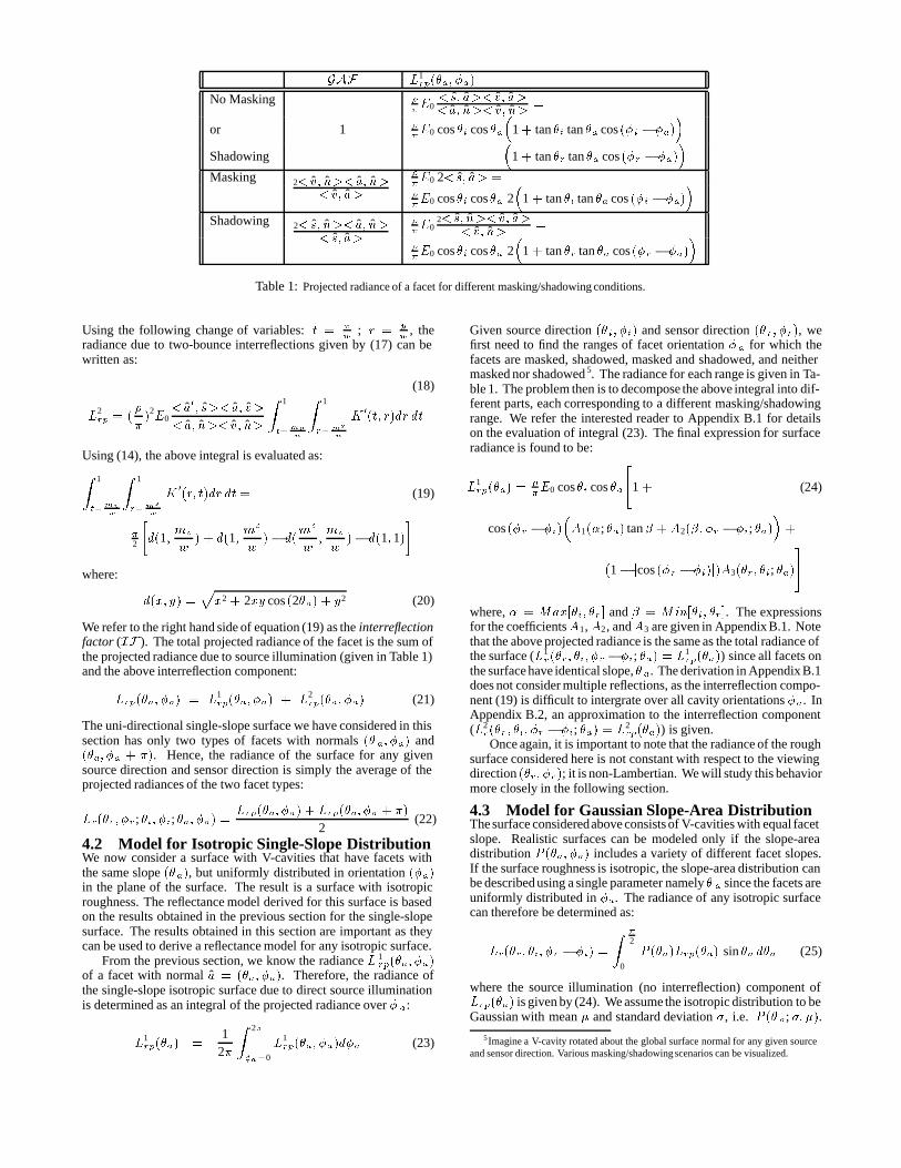
4.1.2 Interreflection Factor

In our reflectance model, we also account for interreflections; lightrays bouncing between adjacent facets. These effects are signifi-cant for rough surfaces with relatively high albedo values. Whenthe surface is illuminated from large angles (�i) and viewed fromthe opposite side at large angles (�r ), none of the facets that are vis-ible to the sensor are illuminated by the source. If interreflectionsare not considered, the radiance of the surface would be zero in thiscase. However, the visible facets receive light from their adjacentfacets that face the source and hence are illuminated. These inter-reflections result in non-zero surface radiance. Our analysis andexperimental results suggest that the contribution due to interreflec-tions can be significant and cannot in general be ignored.

We have the task of modeling interreflections in the presenceof masking and shadowing effects. In the case of Lambertiansurfaces, the energy in an incident light ray diminishes rapidly witheach interreflection bounce. Therefore, we model only two-bounce

interreflections and ignore subsequent bounces. Simulations of theinterreflection process were used to verify that this approximationis good.

In the following discussion, we refer to surface radiance due todirect illumination by the source as L1

r and radiance due to inter-reflections as L2

r . We will use the same superscripts for projectedradiance. The two-bounce interreflection component for a Lamber-tian facet can be expressed as [29] [18] [9] [22]:

L2r�x� �

�

�

Z ZK�x� y�L1

r�y�dy (12)

where x is a point on the facet whose interreflection componentis determined as an integral of the radiance of all points y on theadjacent facet. K�x� y� is the kernel and represents the geometricalrelationship between x and y. Since the V-cavity is long comparedto its width, it can be viewed as a one-dimensional shape with trans-lational symmetry. For such shapes, the interreflection componentcan be determined as an integral over the one-dimensional cross-section of the shape. The above interreflection equation is thereforereduced to:

L2r�x� �

�

�

ZK ��x� y�L1

r�y�dy �13�

where x and y are the shortest distances of points x and y from theintersection of the two facets (see Figure 7). K � is the kernel forthe translational symmetry case and is derived in [16] and [9] to be:

K ��x� y� �� sin2 �2�a�

2xy

�x2 � 2xy cos �2�a� � y2�3�2�14�

We know that the normal of the considered facet is a � ��a� �a�

x

z

yx

^s

^

v

Figure 7: Interreflections in a V-cavity.

and the normal of the adjacent facet is a � � ��a� �a � ��. Thelimits of the integral in the interreflection equation are determinedby the masking and shadowing of these facets. As before, let m v

be the width of the facet which is visible to the viewer. Let ms bethe width of the adjacent facet that is illuminated. As in Section4.1.1, expressions can be obtained for the visible and illuminatedsections:

mv

w�Max

h0�Min

h1���a�� v�

�a� v�

ii(15)

ms

w� Max

h0�Min

h1�� �a� s�

�a�� s�

ii(16)

From the definition of projected radiance (7) and expression (13)we have:

L2rp �

l�a� v�

da �a� n��v� n�

Z w

x�mv

L2r�x�dx � (17)

��

��2E0

l �a�� s��a� v�

da �a� n��v� n�

Z w

x�mv

Z w

y�ms

K ��x� y�dy dx

GAF L1rp��a� �a�

No Masking ��E0

�s� a��v� a��a� n��v� n� �

or 1 ��E0 cos�i cos�a

�1 � tan �i tan �a cos ��i � �a�

�Shadowing

�1 � tan �r tan �a cos ��r � �a�

�Masking 2�v� n��a� n�

�v� a�

��E0 2�s� a� �

��E0 cos�i cos�a 2

�1 � tan �i tan �a cos ��i � �a�

�Shadowing 2�s� n��a� n�

�s� a�

��E0

2�s� n��v� a��v� n�

�

��E0 cos�i cos�a 2

�1 � tan �r tan �a cos ��r � �a�

�Table 1: Projected radiance of a facet for different masking/shadowing conditions.

Using the following change of variables: t � xw ; r � y

w , theradiance due to two-bounce interreflections given by (17) can bewritten as:

(18)

L2rp � �

�

��2E0

�a�� s��a� v�

�a� n��v� n�

Z 1

t�mvw

Z 1

r�ms

w

K ��t� r�dr dt

Using (14), the above integral is evaluated as:Z 1

t�mvw

Z 1

r�ms

w

K ��r� t�dr dt � (19)

�2

�d�1�

mv

w� � d�1�

ms

w�� d�

ms

w�mv

w�� d�1�1�

�

where:

d�x�y� �px2 � 2xy cos �2�a� � y2 (20)

We refer to the right hand side of equation (19) as the interreflectionfactor (IF). The total projected radiance of the facet is the sum ofthe projected radiance due to source illumination (given in Table 1)and the above interreflection component:

Lrp��a� �a� � L1rp��a� �a� � L2

rp��a� �a� (21)

The uni-directional single-slope surface we have considered in thissection has only two types of facets with normals ��a� �a� and��a� �a � ��. Hence, the radiance of the surface for any givensource direction and sensor direction is simply the average of theprojected radiances of the two facet types:

Lr��r� �r ; �i� �i; �a� �a� �Lrp��a� �a� � Lrp��a� �a � ��

2(22)

4.2 Model for Isotropic Single-Slope DistributionWe now consider a surface with V-cavities that have facets withthe same slope ��a�, but uniformly distributed in orientation ��a�in the plane of the surface. The result is a surface with isotropicroughness. The reflectance model derived for this surface is basedon the results obtained in the previous section for the single-slopesurface. The results obtained in this section are important as theycan be used to derive a reflectance model for any isotropic surface.

From the previous section, we know the radiance L 1rp��a� �a�

of a facet with normal a � ��a� �a�. Therefore, the radiance ofthe single-slope isotropic surface due to direct source illuminationis determined as an integral of the projected radiance over � a:

L1rp��a� �

12�

Z 2�

�a�0

L1rp��a� �a�d�a (23)

Given source direction ��i� �i� and sensor direction ��r� �r�, wefirst need to find the ranges of facet orientation �a for which thefacets are masked, shadowed, masked and shadowed, and neithermasked nor shadowed 5. The radiance for each range is given in Ta-ble 1. The problem then is to decompose the above integral into dif-ferent parts, each corresponding to a different masking/shadowingrange. We refer the interested reader to Appendix B.1 for detailson the evaluation of integral (23). The final expression for surfaceradiance is found to be:

L1rp��a� �

��E0 cos�i cos �a

�1 � (24)

cos ��r � �i��A1�; �a� tan� � A2��� �r � �i; �a�

��

�1� jcos ��r � �i�j�A3��r� �i; �a�

�

where, � Max��i� �r � and � � Min��i� �r�. The expressionsfor the coefficientsA1,A2, andA3 are given in Appendix B.1. Notethat the above projected radiance is the same as the total radiance ofthe surface (L1

r��r� �i� �r � �i; �a� � L1rp��a�) since all facets on

the surface have identical slope, �a. The derivation in Appendix B.1does not consider multiple reflections, as the interreflection compo-nent (19) is difficult to intergrate over all cavity orientations �a. InAppendix B.2, an approximation to the interreflection component(L2

r��r � �i� �r � �i; �a� � L2rp��a�) is given.

Once again, it is important to note that the radiance of the roughsurface considered here is not constant with respect to the viewingdirection ��r� �r�; it is non-Lambertian. We will study this behaviormore closely in the following section.

4.3 Model for Gaussian Slope-Area DistributionThe surface consideredabove consists of V-cavities with equal facetslope. Realistic surfaces can be modeled only if the slope-areadistribution P ��a� �a� includes a variety of different facet slopes.If the surface roughness is isotropic, the slope-area distribution canbe described using a single parameter namely � a since the facets areuniformly distributed in �a. The radiance of any isotropic surfacecan therefore be determined as:

Lr��r � �i� �r � �i� �

Z �2

0

P ��a�Lrp��a� sin �a d�a (25)

where the source illumination (no interreflection) component ofLrp��a� is given by (24). We assume the isotropic distribution to beGaussian with mean � and standard deviation , i.e. P �� a; � ��.

5Imagine a V-cavity rotated about the global surface normal for any given sourceand sensor direction. Various masking/shadowing scenarios can be visualized.

Reasonably rough surfaces can be described using a zero mean�� � 0� Gaussian distribution:

P ��a� � c e�

�2a

2�2 (26)

where the normalization constant c is:

1�c �

Z �2

�a�0

Z 2�

�a�0

e�

�2a

2�2 sin �a d�a d�a

The reflectance model is to be obtained by substituting theradiance L1

rp��a� given by (24) and the Gaussian distributionP ��a; � 0� in integral (25). The resulting integral cannot be easilyevaluated. Therefore, we pursued a functional approximation to theintegral that is accurate for arbitrary surface roughnessand angles ofincidence and reflection. In deriving this approximation, we care-fully studied the functional form of L1

rp��a� given by (24). Thisenabled us to identify basis functions that can be used in the approx-imation. Then, we conducted a large set of numerical evaluationsof the integral in (25) by varying surface roughness , the anglesof incidence ��i� �i� and reflection ��r� �r�. These simulationsand the identified basis functions were used to arrive at an accuratefunctional approximation for surface radiance. This procedure wasapplied independently to the direct illumination component as wellas the interreflection component.

The final approximation results are given below. Once again,let � Max��r� �i� and� �Min��r � �i�. The direct illuminationcomponent of radiance of a surface with roughness is:

L1r��r � �i� �r � �i; �� �

��E0 cos �i

�C1��� � (27)

cos ��r � �i�C2��;�;�r � �i ; �� tan� ��1� j cos ��r � �i�j

�C3��;�; �� tan

��� �

2

��

where the coefficients are:

C1 � 1� 0�5�2

�2 � 0�33

C2 �

���

0�45 �2

�2�0�09sin� if cos ��r � �i� � 0

0�45 �2

�2�0�09

sin�� � 2�

��3

otherwise

C3 � 0�125

�2

�2 � 0�09

4��

2

2

Using a similar approach, an approximation to the interreflectioncomponent was also derived. In this case, the interreflection com-ponent for the single-slope isotropic surface (Appendix B.2) wasused to guess the basis functions. The final approximation to theinterreflection component of radiance for a surface with roughness is:

L2r��r � �i� �r � �i; � � (28)

0�17�2

�E0 cos�i

2

2 � 0�13

�1� cos ��r � �i�

2��

2�

The two components are combined to obtain the total surface radi-ance:

Lr��r� �i� �r � �i; � � (29)

L1r��r� �i� �r � �i; � � L2

r��r � �i� �r � �i; �

If the surface is extremely rough, causing the zero-mean Gaussianmodel to be an inaccurate approximation, an additional param-eter can be used to weight the interreflection component. Oursimulations show that this enables the model to stretch a bit be-yond its theoretical limits. Finally, the BRDF of the surface is ob-tained from its radiance and irradiance as fr��r � �i� �r � �i; � �Lr��r� �i� �r � �i; � �E0 cos �i. It is important to note that theabovemodel obeysHelmholtz’s reciprocity principle (see [2]). Alsonote that the model reduces to the Lambertian model 6 when � 0.Note that by substituting the albedo as function of the wavelength,����, the dependency of the model on the wavelength comes outexplicitly.

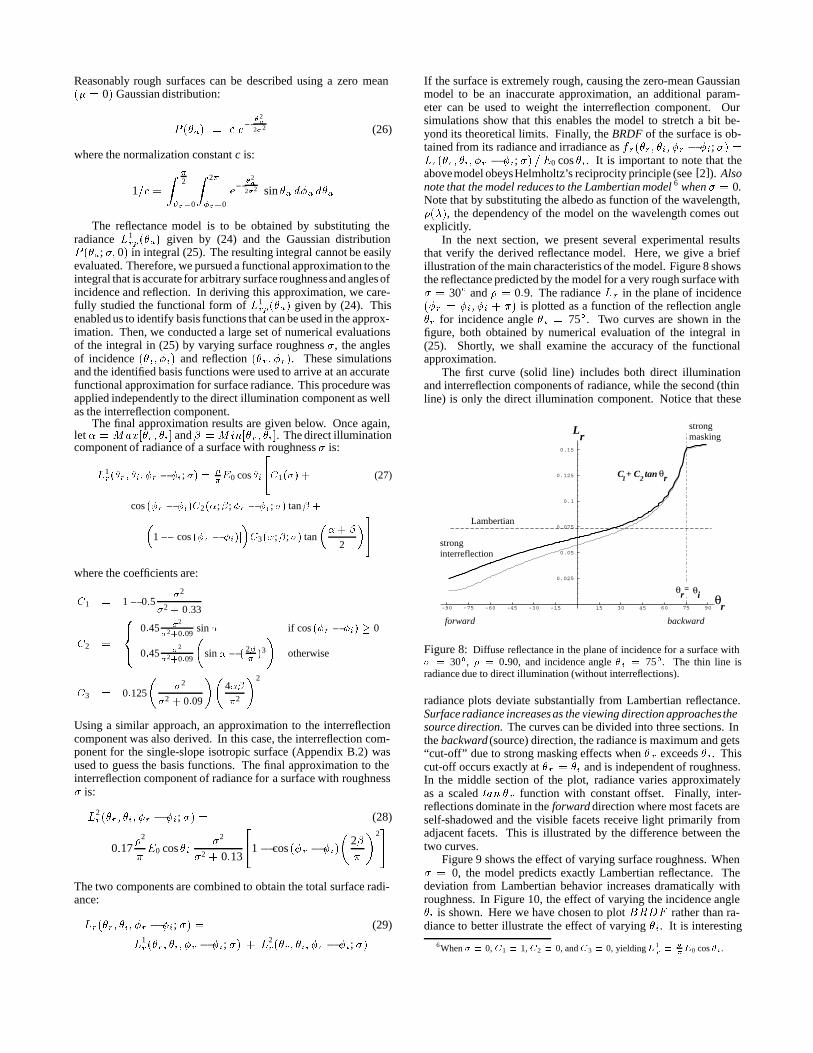
In the next section, we present several experimental resultsthat verify the derived reflectance model. Here, we give a briefillustration of the main characteristics of the model. Figure 8 showsthe reflectance predicted by the model for a very rough surface with � 30� and � � 0�9. The radiance Lr in the plane of incidence��r � �i� �i � �� is plotted as a function of the reflection angle�r for incidence angle �i � 75�. Two curves are shown in thefigure, both obtained by numerical evaluation of the integral in(25). Shortly, we shall examine the accuracy of the functionalapproximation.

The first curve (solid line) includes both direct illuminationand interreflection components of radiance, while the second (thinline) is only the direct illumination component. Notice that these

-90 -75 -60 -45 -30 -15 15 30 45 60 75 90

0.025

0.05

0.075

0.1

0.125

0.15

Lr

rθiθrθ =

strong masking

strong interreflection

Lambertian

C + C tan rθ1 2

forward backward

Figure 8: Diffuse reflectance in the plane of incidence for a surface with� � 30�, � 0�90, and incidence angle � i � 75�. The thin line isradiance due to direct illumination (without interreflections).

radiance plots deviate substantially from Lambertian reflectance.Surface radiance increases as the viewing direction approaches thesource direction. The curves can be divided into three sections. Inthe backward (source) direction, the radiance is maximum and gets“cut-off” due to strong masking effects when � r exceeds �i. Thiscut-off occurs exactly at �r � �i and is independent of roughness.In the middle section of the plot, radiance varies approximatelyas a scaled tan �r function with constant offset. Finally, inter-reflections dominate in the forward direction where most facets areself-shadowed and the visible facets receive light primarily fromadjacent facets. This is illustrated by the difference between thetwo curves.

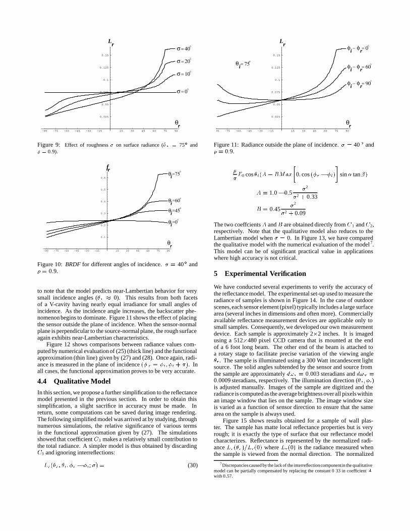
Figure 9 shows the effect of varying surface roughness. When � 0, the model predicts exactly Lambertian reflectance. Thedeviation from Lambertian behavior increases dramatically withroughness. In Figure 10, the effect of varying the incidence angle�i is shown. Here we have chosen to plot BRDF rather than ra-diance to better illustrate the effect of varying �i. It is interesting

6When � � 0, C1 � 1, C2 � 0, andC3 � 0, yieldingL1r � �

�E0 cos �i.

-90 -75 -60 -45 -30 -15 15 30 45 60 75 90

0.025

0.05

0.075

0.1

0.125

0.15

Lr

rθ

σ = 40

σ = 20

σ = 10

σ = 0

Figure 9: Effect of roughness � on surface radiance (� i � 75� and � 0�9).

-90 -75 -60 -45 -30 -15 15 30 45 60 75 90

0.1

0.2

0.3

0.4

0.5

0.6

fr

rθ

iθ =75

iθ =60

iθ =45

iθ =0

Figure 10: BRDF for different angles of incidence. � 40� and� � 0�9.

to note that the model predicts near-Lambertian behavior for verysmall incidence angles (�i � 0). This results from both facetsof a V-cavity having nearly equal irradiance for small angles ofincidence. As the incidence angle increases, the backscatter phe-nomenon begins to dominate. Figure 11 shows the effect of placingthe sensor outside the plane of incidence. When the sensor-normalplane is perpendicular to the source-normal plane, the rough surfaceagain exhibits near-Lambertian characteristics.

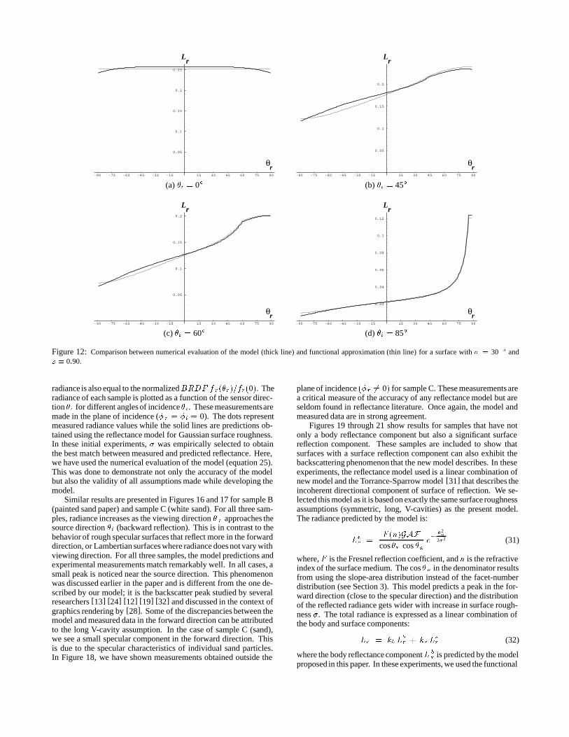
Figure 12 shows comparisons between radiance values com-puted by numerical evaluation of (25) (thick line) and the functionalapproximation (thin line) given by (27) and (28). Once again, radi-ance is measured in the plane of incidence �� r � �i� �i � ��. Inall cases, the functional approximation proves to be very accurate.

4.4 Qualitative Model

In this section, we propose a further simplification to the reflectancemodel presented in the previous section. In order to obtain thissimplification, a slight sacrifice in accuracy must be made. Inreturn, some computations can be saved during image rendering.The following simplified model was arrived at by studying, throughnumerous simulations, the relative significance of various termsin the functional approximation given by (27). The simulationsshowed that coefficientC3 makes a relatively small contribution tothe total radiance. A simpler model is thus obtained by discardingC3 and ignoring interreflections:

Lr��r� �i� �r � �i; � � (30)

90 -75 -60 -45 -30 -15 15 30 45 60 75 90

0.025

0.05

0.075

0.1

0.125

0.15iφ rφ− = 0

iφ rφ− = 60

iφ rφ− = 90

Lr

rθ

iθ = 75

Figure 11: Radiance outside the plane of incidence. � 40 � and� � 0�9.

�

�E0 cos�i�A� BMax

�0� cos ��r � �i�

�sin tan��

A � 1�0� 0�5 2

2 � 0�33

B � 0�45 2

2 � 0�09

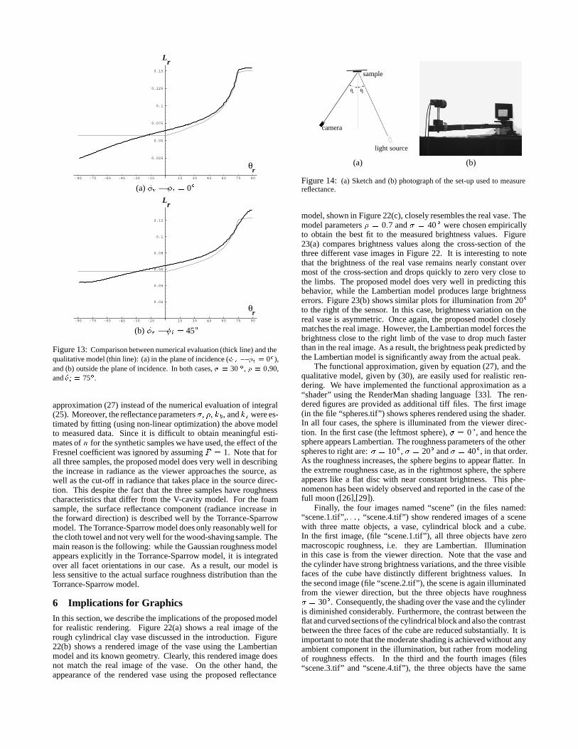
The two coeffcientsA andB are obtained directly fromC 1 andC2,respectively. Note that the qualitative model also reduces to theLambertian model when � 0. In Figure 13, we have comparedthe qualitative model with the numerical evaluation of the model 7.This model can be of significant practical value in applicationswhere high accuracy is not critical.

5 Experimental Verification

We have conducted several experiments to verify the accuracy ofthe reflectance model. The experimental set-up used to measure theradiance of samples is shown in Figure 14. In the case of outdoorscenes,each sensor element (pixel) typically includes a large surfacearea (several inches in dimensions and often more). Commerciallyavailable reflectance measurement devices are applicable only tosmall samples. Consequently, we developed our own measurementdevice. Each sample is approximately 2�2 inches. It is imagedusing a 512�480 pixel CCD camera that is mounted at the endof a 6 foot long beam. The other end of the beam is attached toa rotary stage to facilitate precise variation of the viewing angle�r . The sample is illuminated using a 300 Watt incandescent lightsource. The solid angles subtended by the sensor and source fromthe sample are approximately d�i � 0�003 steradians and d�r �0�0009 steradians, respectively. The illumination direction (� i� �i)is adjusted manually. Images of the sample are digitized and theradianceis computed as the average brightness over all pixels withinan image window that lies on the sample. The image window sizeis varied as a function of sensor direction to ensure that the samearea on the sample is always used.

Figure 15 shows results obtained for a sample of wall plas-ter. The sample has matte local reflectance properties but is veryrough; it is exactly the type of surface that our reflectance modelcharacterizes. Reflectance is represented by the normalized radi-ance Lr��r��Lr�0� where Lr�0� is the radiance measured whenthe sample is viewed from the normal direction. The normalized

7Discrepancies caused by the lack of the interreflection componentin the qualitativemodel can be partially compensated by replacing the constant 0�33 in coefficient Awith 0�57.

Lr

rθ-90 -75 -60 -45 -30 -15 15 30 45 60 75 90

0.05

0.1

0.15

0.2

0.25

Lr

rθ-90 -75 -60 -45 -30 -15 15 30 45 60 75 90

0.05

0.1

0.15

0.2

(a) �i � 0� (b) �i � 45�

Lr

rθ-90 -75 -60 -45 -30 -15 15 30 45 60 75 90

0.05

0.1

0.15

0.2

Lr

rθ-90 -75 -60 -45 -30 -15 15 30 45 60 75 90

0.02

0.04

0.06

0.08

0.1

0.12

(c) �i � 60� (d) �i � 85�

Figure 12: Comparison between numerical evaluation of the model (thick line) and functional approximation (thin line) for a surface with � � 30 � and � 0�90.

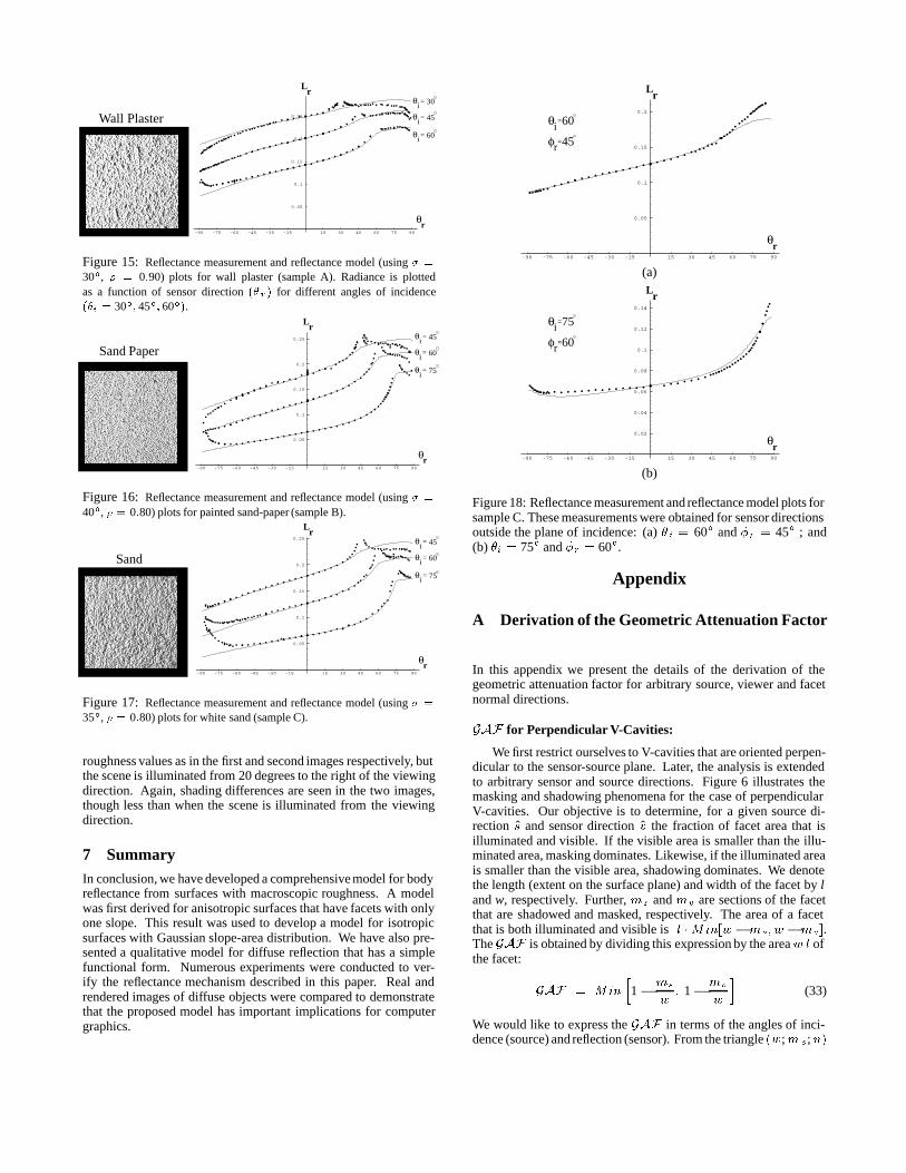
radiance is also equal to the normalizedBRDF f r��r��fr�0�. Theradiance of each sample is plotted as a function of the sensor direc-tion �r for different angles of incidence�i. These measurementsaremade in the plane of incidence (�r � �i � 0). The dots representmeasured radiance values while the solid lines are predictions ob-tained using the reflectance model for Gaussian surface roughness.In these initial experiments, was empirically selected to obtainthe best match between measured and predicted reflectance. Here,we have used the numerical evaluation of the model (equation 25).This was done to demonstrate not only the accuracy of the modelbut also the validity of all assumptions made while developing themodel.

Similar results are presented in Figures 16 and 17 for sample B(painted sand paper) and sample C (white sand). For all three sam-ples, radiance increases as the viewing direction � r approaches thesource direction �i (backward reflection). This is in contrast to thebehavior of rough specular surfaces that reflect more in the forwarddirection, or Lambertian surfaces where radiance does not vary withviewing direction. For all three samples, the model predictions andexperimental measurements match remarkably well. In all cases, asmall peak is noticed near the source direction. This phenomenonwas discussed earlier in the paper and is different from the one de-scribed by our model; it is the backscatter peak studied by severalresearchers [13] [24] [12] [19] [32] and discussed in the context ofgraphics rendering by [28]. Some of the discrepancies between themodel and measured data in the forward direction can be attributedto the long V-cavity assumption. In the case of sample C (sand),we see a small specular component in the forward direction. Thisis due to the specular characteristics of individual sand particles.In Figure 18, we have shown measurements obtained outside the

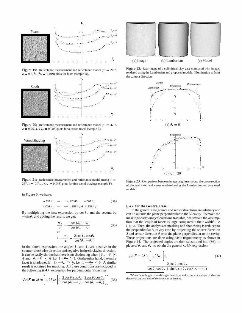
plane of incidence ��r �� 0� for sample C. These measurements area critical measure of the accuracy of any reflectance model but areseldom found in reflectance literature. Once again, the model andmeasured data are in strong agreement.

Figures 19 through 21 show results for samples that have notonly a body reflectance component but also a significant surfacereflection component. These samples are included to show thatsurfaces with a surface reflection component can also exhibit thebackscattering phenomenon that the new model describes. In theseexperiments, the reflectance model used is a linear combination ofnew model and the Torrance-Sparrow model [31] that describes theincoherent directional component of surface of reflection. We se-lected this model as it is based on exactly the same surface roughnessassumptions (symmetric, long, V-cavities) as the present model.The radiance predicted by the model is:

Lsr �F �n�GAF

cos�r cos �ae�

�2a

2�2 (31)

where,F is the Fresnel reflection coefficient, andn is the refractiveindex of the surface medium. The cos�a in the denominator resultsfrom using the slope-area distribution instead of the facet-numberdistribution (see Section 3). This model predicts a peak in the for-ward direction (close to the specular direction) and the distributionof the reflected radiance gets wider with increase in surface rough-ness . The total radiance is expressed as a linear combination ofthe body and surface components:

Lr � kb Lbr � ks L

sr (32)

where the body reflectance componentL br is predicted by the model

proposed in this paper. In these experiments, we used the functional

Lr

rθ-90 -75 -60 -45 -30 -15 15 30 45 60 75 90

0.025

0.05

0.075

0.1

0.125

0.15

(a) �r � �i � 0�

Lr

rθ-90 -75 -60 -45 -30 -15 15 30 45 60 75 90

0.02

0.04

0.06

0.08

0.1

0.12

(b) �r � �i � 45�

Figure 13: Comparison between numerical evaluation (thick line) and thequalitative model (thin line): (a) in the plane of incidence (� r � �i � 0�),and (b) outside the plane of incidence. In both cases, � � 30 �, � 0�90,and �i � 75�.

approximation (27) instead of the numerical evaluation of integral(25). Moreover, the reflectance parameters , �, kb, and ks were es-timated by fitting (using non-linear optimization) the above modelto measured data. Since it is difficult to obtain meaningful esti-mates of n for the synthetic samples we have used, the effect of theFresnel coefficient was ignored by assuming F � 1. Note that forall three samples, the proposed model does very well in describingthe increase in radiance as the viewer approaches the source, aswell as the cut-off in radiance that takes place in the source direc-tion. This despite the fact that the three samples have roughnesscharacteristics that differ from the V-cavity model. For the foamsample, the surface reflectance component (radiance increase inthe forward direction) is described well by the Torrance-Sparrowmodel. The Torrance-Sparrow model does only reasonably well forthe cloth towel and not very well for the wood-shaving sample. Themain reason is the following: while the Gaussian roughness modelappears explicitly in the Torrance-Sparrow model, it is integratedover all facet orientations in our case. As a result, our model isless sensitive to the actual surface roughness distribution than theTorrance-Sparrow model.

6 Implications for GraphicsIn this section, we describe the implications of the proposed modelfor realistic rendering. Figure 22(a) shows a real image of therough cylindrical clay vase discussed in the introduction. Figure22(b) shows a rendered image of the vase using the Lambertianmodel and its known geometry. Clearly, this rendered image doesnot match the real image of the vase. On the other hand, theappearance of the rendered vase using the proposed reflectance

camera

light source

sample

θr θi

(a) (b)

Figure 14: (a) Sketch and (b) photograph of the set-up used to measurereflectance.

model, shown in Figure 22(c), closely resembles the real vase. Themodel parameters � � 0�7 and � 40� were chosen empiricallyto obtain the best fit to the measured brightness values. Figure23(a) compares brightness values along the cross-section of thethree different vase images in Figure 22. It is interesting to notethat the brightness of the real vase remains nearly constant overmost of the cross-section and drops quickly to zero very close tothe limbs. The proposed model does very well in predicting thisbehavior, while the Lambertian model produces large brightnesserrors. Figure 23(b) shows similar plots for illumination from 20�

to the right of the sensor. In this case, brightness variation on thereal vase is asymmetric. Once again, the proposed model closelymatches the real image. However, the Lambertian model forces thebrightness close to the right limb of the vase to drop much fasterthan in the real image. As a result, the brightness peak predicted bythe Lambertian model is significantly away from the actual peak.

The functional approximation, given by equation (27), and thequalitative model, given by (30), are easily used for realistic ren-dering. We have implemented the functional approximation as a“shader” using the RenderMan shading language [33]. The ren-dered figures are provided as additional tiff files. The first image(in the file “spheres.tif”) shows spheres rendered using the shader.In all four cases, the sphere is illuminated from the viewer direc-tion. In the first case (the leftmost sphere), � 0�, and hence thesphere appears Lambertian. The roughness parameters of the otherspheres to right are: � 10�, � 20� and � 40�, in that order.As the roughness increases, the sphere begins to appear flatter. Inthe extreme roughness case, as in the rightmost sphere, the sphereappears like a flat disc with near constant brightness. This phe-nomenon has been widely observed and reported in the case of thefull moon ([26],[29]).

Finally, the four images named “scene” (in the files named:“scene.1.tif”,� � � , “scene.4.tif”) show rendered images of a scenewith three matte objects, a vase, cylindrical block and a cube.In the first image, (file “scene.1.tif”), all three objects have zeromacroscopic roughness, i.e. they are Lambertian. Illuminationin this case is from the viewer direction. Note that the vase andthe cylinder have strong brightness variations, and the three visiblefaces of the cube have distinctly different brightness values. Inthe second image (file “scene.2.tif”), the scene is again illuminatedfrom the viewer direction, but the three objects have roughness � 30�. Consequently, the shading over the vase and the cylinderis diminished considerably. Furthermore, the contrast between theflat and curved sections of the cylindrical block and also the contrastbetween the three faces of the cube are reduced substantially. It isimportant to note that the moderate shading is achieved without anyambient component in the illumination, but rather from modelingof roughness effects. In the third and the fourth images (files“scene.3.tif” and “scene.4.tif”), the three objects have the same

Wall Plaster

Lr

rθ

iθ = 30

iθ = 45

iθ = 60

-90 -75 -60 -45 -30 -15 15 30 45 60 75 90

0.05

0.1

0.15

0.2

0.25

Figure 15: Reflectance measurement and reflectance model (using � �30�, � 0�90) plots for wall plaster (sample A). Radiance is plottedas a function of sensor direction �� r� for different angles of incidence��i � 30�� 45�� 60��.

Sand Paper

Lr

rθ

iθ = 45

iθ = 60

iθ = 75

-90 -75 -60 -45 -30 -15 15 30 45 60 75 90

0.05

0.1

0.15

0.2

0.25

Figure 16: Reflectance measurement and reflectance model (using � �40�, � 0�80) plots for painted sand-paper (sample B).

Sand

Lr

rθ

iθ = 45

iθ = 60

iθ = 75

-90 -75 -60 -45 -30 -15 15 30 45 60 75 90

0.05

0.1

0.15

0.2

0.25

Figure 17: Reflectance measurement and reflectance model (using � �35�, � 0�80) plots for white sand (sample C).

roughness values as in the first and second images respectively, butthe scene is illuminated from 20 degrees to the right of the viewingdirection. Again, shading differences are seen in the two images,though less than when the scene is illuminated from the viewingdirection.

7 SummaryIn conclusion, we have developed a comprehensive model for bodyreflectance from surfaces with macroscopic roughness. A modelwas first derived for anisotropic surfaces that have facets with onlyone slope. This result was used to develop a model for isotropicsurfaces with Gaussian slope-area distribution. We have also pre-sented a qualitative model for diffuse reflection that has a simplefunctional form. Numerous experiments were conducted to ver-ify the reflectance mechanism described in this paper. Real andrendered images of diffuse objects were compared to demonstratethat the proposed model has important implications for computergraphics.

Lr

rθ

iθ 60=

rφ 45=

-90 -75 -60 -45 -30 -15 15 30 45 60 75 90

0.05

0.1

0.15

0.2

(a)Lr

rθ-90 -75 -60 -45 -30 -15 15 30 45 60 75 90

0.02

0.04

0.06

0.08

0.1

0.12

0.14

iθ 75=

rφ 60=

(b)

Figure 18: Reflectance measurement and reflectance model plots forsample C. These measurements were obtained for sensor directionsoutside the plane of incidence: (a) � i � 60� and �r � 45� ; and(b) �i � 75� and �r � 60�.

Appendix

A Derivation of the Geometric Attenuation Factor

In this appendix we present the details of the derivation of thegeometric attenuation factor for arbitrary source, viewer and facetnormal directions.

GAF for Perpendicular V-Cavities:

We first restrict ourselves to V-cavities that are oriented perpen-dicular to the sensor-source plane. Later, the analysis is extendedto arbitrary sensor and source directions. Figure 6 illustrates themasking and shadowing phenomena for the case of perpendicularV-cavities. Our objective is to determine, for a given source di-rection s and sensor direction v the fraction of facet area that isilluminated and visible. If the visible area is smaller than the illu-minated area, masking dominates. Likewise, if the illuminated areais smaller than the visible area, shadowing dominates. We denotethe length (extent on the surface plane) and width of the facet by land w, respectively. Further, ms and mv are sections of the facetthat are shadowed and masked, respectively. The area of a facetthat is both illuminated and visible is l �Min�w �ms� w �mv�.The GAF is obtained by dividing this expression by the areaw l ofthe facet:

GAF � Minh

1� ms

w� 1� mv

w

i(33)

We would like to express the GAF in terms of the angles of inci-dence (source) and reflection (sensor). From the triangle �w;m s; n�

Foam

Lr

rθ

iθ = 45

iθ = 60

iθ = 75

-90 -75 -60 -45 -30 -15 15 30 45 60 75 90

0.05

0.1

0.15

0.2

Figure 19: Reflectance measurement and reflectance model (� � 20 �, � 0�8, ks�kb � 0�019) plots for foam (sample D).

Cloth

-90 -75 -60 -45 -30 -15 15 30 45 60 75 90

0.05

0.1

0.15

0.2

Lr

rθ

iθ = 45

iθ = 60

iθ = 75

Figure 20: Reflectance measurement and reflectance model (� � 42 �, � 0�75, ks�kb � 0�085) plots for a cotton towel (sample E).

Wood Shaving

-90 -75 -60 -45 -30 -15 15 30 45 60 75 90

0.05

0.1

0.15

0.2

Lr

rθ

iθ = 45

iθ = 60

iθ = 75

Figure 21: Reflectance measurement and reflectance model (using � �26�, � 0�7, ks�kb � 0�043) plots for fine wood shavings (sample F).

in Figure 6, we have:

n sin �i � ms cos�a � w cos �a (34)

n cos �i � �ms sin �a � w sin �a

By multiplying the first expression by cos� i and the second by� sin �i and adding the results we get:

ms

w� � cos ��a � �i�

cos ��a � �i�(35)

or

1� ms

w�

2 cos�a cos �icos ��a � �i�

In the above expression, the angles � i and �r are positive in thecounter-clockwise direction and negative in the clockwise direction.It can be easily shown that there is no shadowing when j � a��i j��2 and j �a��i j� �

2 , i.e. 1�ms

w� 1. On the other hand, the entire

facet is shadowed if j �i � �a j� �2 , i.e. 1� ms

w � 0. A similarresult is obtained for masking. All these conditions are included inthe following GAF expression for perpendicular V-cavities:

GAF � Min

�1�Max

�0�

2 cos�icos�acos ��i � �a�

�2 cos�rcos�acos ��r � �a�

��(36)

(a) Image (b) Lambertian (c) Model

Figure 22: Real image of a cylindrical clay vase compared with imagesrendered using the Lambertian and proposed models. Illumination is fromthe camera direction.

Lambertian

ModelMeasurements

Brightness

X

(a) �i � 0�

Brightness

X

(b) �i � 20�

Figure 23: Comparison between image brightness along the cross-sectionof the real vase, and vases rendered using the Lambertian and proposedmodels.

GAF for the General Case:In the general case,source and sensor directions are arbitrary and

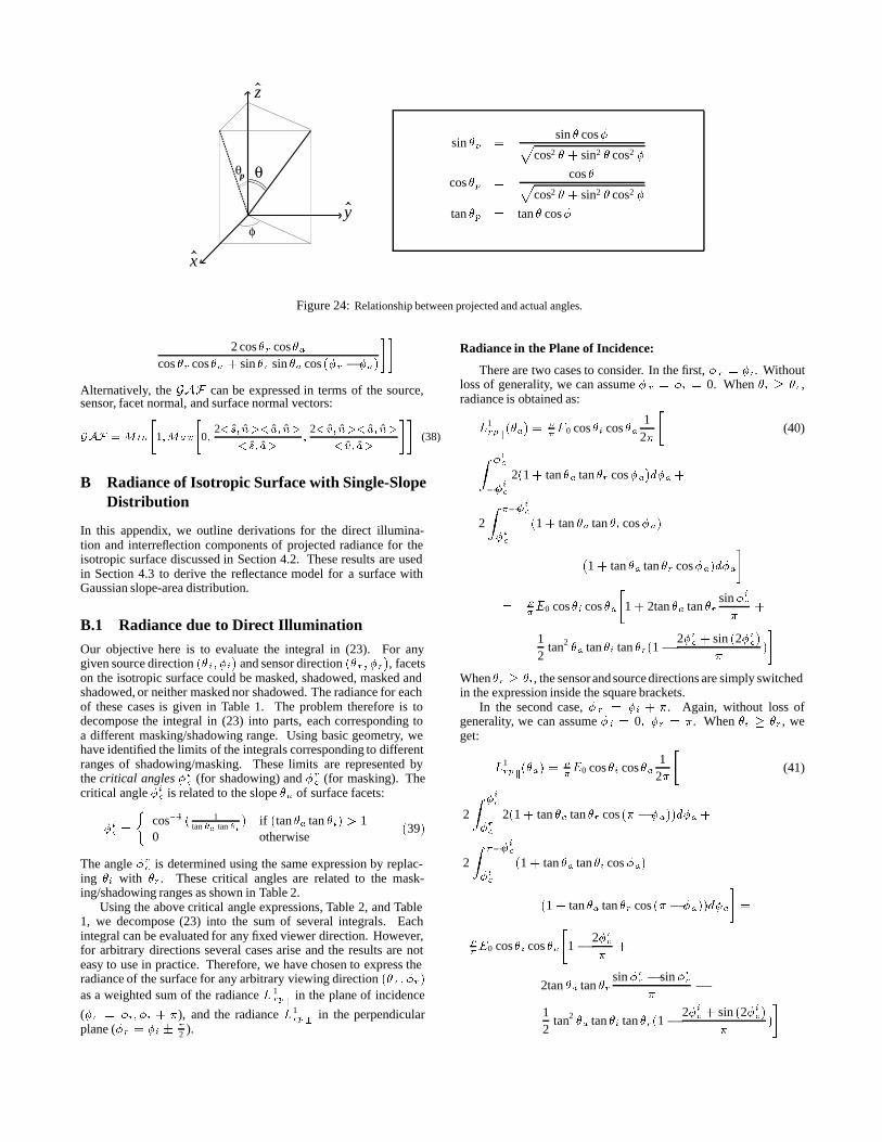
can lie outside the plane perpendicular to the V-cavity. To make themasking/shadowing calculations tractable, we invoke the assump-tion that the length of facets is large compared to their width8, i.e.l� w. Then, the analysis of masking and shadowing is reduced tothe perpendicular V-cavity case by projecting the source directions and sensor direction v onto the plane perpendicular to the cavity.These projections are done using basic trigonometry as shown inFigure 24. The projected angles are then substituted into (36), inplace of �i and �r , to obtain the general GAF expression:

GAF �Min

�1�Max

�0� (37)

2 cos�i cos�acos�i cos�a � sin �i sin �a cos ��i � �a�

�

8When facet length is much larger than facet width, the exact shape of the castshadow at the two ends of the facet can be ignored.

θθp

φ

x

y

z

^

^

sin �p �sin � cos�p

cos2 � � sin2 � cos2 �

cos�p �cos �p

cos2 � � sin2 � cos2 �

tan �p � tan � cos�

Figure 24: Relationship between projected and actual angles.

2 cos�r cos�acos �r cos�a � sin �r sin �a cos ��r � �a�

��

Alternatively, the GAF can be expressed in terms of the source,sensor, facet normal, and surface normal vectors:

GAF �Min

�1�Max

�0�

2�s� n��a� n�

�s� a��

2�v� n��a� n�

�v� a�

��(38)

B Radiance of Isotropic Surface with Single-SlopeDistribution

In this appendix, we outline derivations for the direct illumina-tion and interreflection components of projected radiance for theisotropic surface discussed in Section 4.2. These results are usedin Section 4.3 to derive the reflectance model for a surface withGaussian slope-area distribution.

B.1 Radiance due to Direct Illumination

Our objective here is to evaluate the integral in (23). For anygiven source direction ��i� �i� and sensor direction ��r � �r�, facetson the isotropic surface could be masked, shadowed, masked andshadowed, or neither masked nor shadowed. The radiance for eachof these cases is given in Table 1. The problem therefore is todecompose the integral in (23) into parts, each corresponding toa different masking/shadowing range. Using basic geometry, wehave identified the limits of the integrals corresponding to differentranges of shadowing/masking. These limits are represented bythe critical angles �ic (for shadowing) and �rc (for masking). Thecritical angle �ic is related to the slope �a of surface facets:

�ic �

�cos�1 � 1

tan �a tan �i� if �tan �a tan �i� � 1

0 otherwise�39�

The angle �rc is determined using the same expression by replac-ing �i with �r . These critical angles are related to the mask-ing/shadowing ranges as shown in Table 2.

Using the above critical angle expressions, Table 2, and Table1, we decompose (23) into the sum of several integrals. Eachintegral can be evaluated for any fixed viewer direction. However,for arbitrary directions several cases arise and the results are noteasy to use in practice. Therefore, we have chosen to express theradiance of the surface for any arbitrary viewing direction ��r � �r�as a weighted sum of the radiance L 1

rpk in the plane of incidence

(�r � �i� �i � �), and the radiance L1rp�

in the perpendicularplane (�r � �i �

2 ).

Radiance in the Plane of Incidence:

There are two cases to consider. In the first, �r � �i. Withoutloss of generality, we can assume � r � �i � 0. When �i � �r ,radiance is obtained as:

L1rpk

��a� ���E0 cos�i cos�a

12�

�(40)

Z �ic

��ic2�1 � tan �a tan �r cos�a�d�a �

2

Z ���ic

�ic�1 � tan �a tan �i cos�a�

�1 � tan �a tan �r cos�a�d�a

�

� ��E0 cos�i cos �a

�1 � 2tan �a tan �r

sin�ic�

�

12

tan2 �a tan �i tan �r�1� 2�ic � sin �2�ic��

�

�When�r � �i, the sensor and source directions are simply switchedin the expression inside the square brackets.

In the second case, �r � �i � �. Again, without loss ofgenerality, we can assume � i � 0� �r � �. When �i � �r , weget:

L1rpk��a� �

��E0 cos�i cos�a

12�

�(41)

2

Z �ic

�rc2�1 � tan �a tan �r cos �� � �a��d�a �

2

Z ���ic

�ic�1 � tan �a tan �i cos�a�

�1 � tan �a tan �r cos �� � �a��d�a

��

��E0 cos�i cos �a

�1� 2�rc

��

2tan �a tan �rsin�rc � sin�ic

��

12

tan2 �a tan �i tan �r�1� 2�ic � sin �2�ic��

�

�

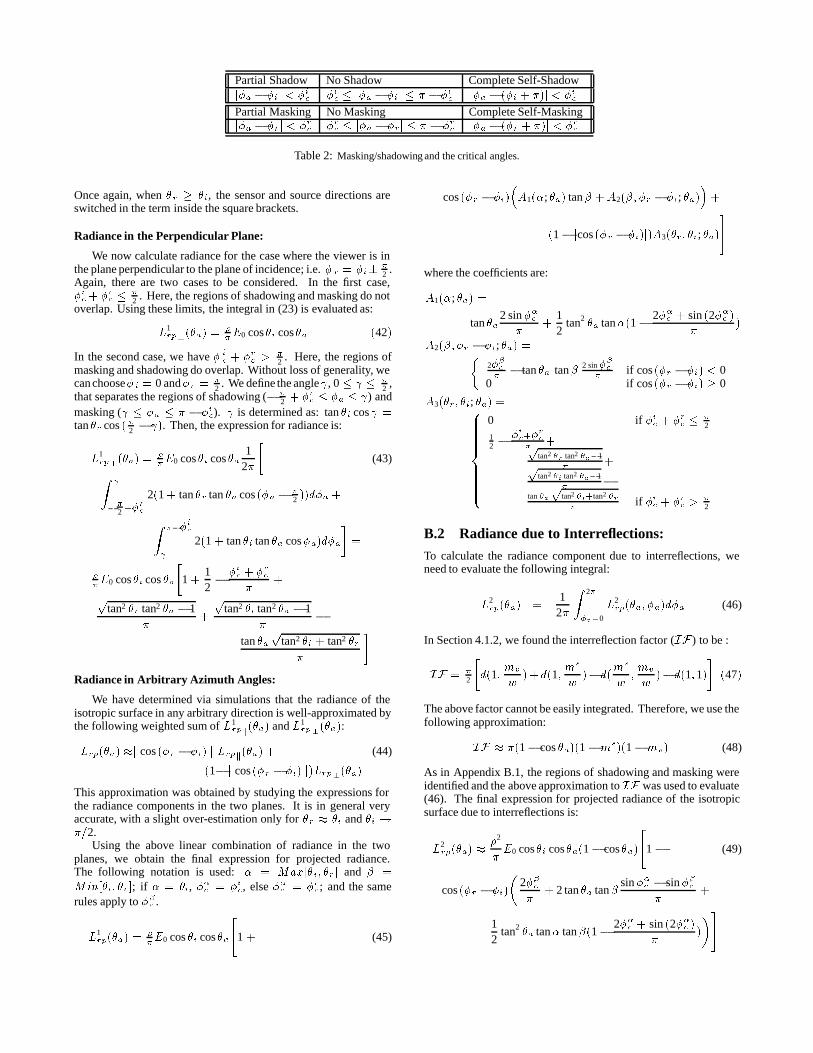
Partial Shadow No Shadow Complete Self-Shadowj�a � �ij � �ic �ic � j�a � �ij � � � �ic j�a � ��i � ��j � �icPartial Masking No Masking Complete Self-Maskingj�a � �rj � �rc �rc � j�a � �rj � � � �rc j�a � ��r � ��j � �rc

Table 2: Masking/shadowing and the critical angles.

Once again, when �r � �i, the sensor and source directions areswitched in the term inside the square brackets.

Radiance in the Perpendicular Plane:

We now calculate radiance for the case where the viewer is inthe plane perpendicular to the plane of incidence; i.e. � r � �i �

2 .Again, there are two cases to be considered. In the first case,�ic � �rc � �

2 . Here, the regions of shadowing and masking do notoverlap. Using these limits, the integral in (23) is evaluated as:

L1rp���a� �

��E0 cos�i cos�a �42�

In the second case, we have � ic � �rc �

�2 . Here, the regions of

masking and shadowing do overlap. Without loss of generality, wecan choose� i � 0 and�r � �

2 . We define the angle�, 0 � � � �2 ,

that separates the regions of shadowing (� �2 � �rc � �a � �) and

masking (� � �a � � � �ic). � is determined as: tan �i cos� �tan �r cos � �2 � ��. Then, the expression for radiance is:

L1rp���a� �

��E0 cos�i cos�a

12�

�(43)Z �

��2 ��

rc

2�1� tan �r tan �a cos ��a � �2 ��d�a �

Z ���ic

�

2�1 � tan �i tan �a cos�a�d�a

��

��E0 cos�i cos �a

�1 �

12� �ic � �rc

��

ptan2 �r tan2 �a � 1

��

ptan2 �i tan2 �a � 1

��

tan �ap

tan2 �i � tan2 �r�

�Radiance in Arbitrary Azimuth Angles:

We have determined via simulations that the radiance of theisotropic surface in any arbitrary direction is well-approximated bythe following weighted sum of L1

rpk��a� and L1

rp���a�:

Lrp��a� �j cos ��r � �i� j Lrpk��a� � (44)

�1� j cos ��r � �i� j�Lrp���a�This approximation was obtained by studying the expressions forthe radiance components in the two planes. It is in general veryaccurate, with a slight over-estimation only for �r � �i and �i ��2.

Using the above linear combination of radiance in the twoplanes, we obtain the final expression for projected radiance.The following notation is used: � Max��i� �r� and � �Min��i� �r�; if � �i, �c � �ic, else �c � �rc; and the samerules apply to ��c .

L1rp��a� �

��E0 cos �i cos�a

�1 � (45)

cos ��r � �i��A1�; �a� tan� �A2��� �r � �i; �a�

��

�1� jcos ��r � �i�j�A3��r� �i; �a�

�

where the coefficients are:

A1�; �a� �

tan �a2 sin�c

��

12

tan2 �a tan�1� 2�c � sin �2�c ��

�

A2����r � �i; �a� ��2��c�� tan �a tan� 2 sin��c

�if cos ��r � �i� � 0

0 if cos ��r � �i� � 0

A3��r� �i; �a� ����������������

0 if �ic � �rc � �2

12 � �ic��

rc

��p

tan2 �r tan2 �a�1�

�ptan2 �i tan2 �a�1

��

tan �ap

tan2 �i�tan2 �r� if �ic � �rc �

�2

B.2 Radiance due to Interreflections:

To calculate the radiance component due to interreflections, weneed to evaluate the following integral:

L2rp��a� �

12�

Z 2�

�a�0

L2rp��a� �a�d�a (46)

In Section 4.1.2, we found the interreflection factor (IF) to be :

IF � �2

�d�1�

mv

w��d�1�

ms

w��d�

ms

w�mv

w��d�1�1�

��47�

The above factor cannot be easily integrated. Therefore, we use thefollowing approximation:

IF � ��1� cos �a��1�ms��1�mv� (48)

As in Appendix B.1, the regions of shadowing and masking wereidentified and the above approximation to IF was used to evaluate(46). The final expression for projected radiance of the isotropicsurface due to interreflections is:

L2rp��a� � �2

�E0 cos�i cos�a�1� cos�a�

�1� (49)

cos ��r � �i�

2��c�

� 2 tan �a tan�sin�c � sin��c

��

12

tan2 �a tan tan��1� 2�c � sin �2�c ��

�

�

REFERENCES

[1] P. Beckmann. Shadowing of random rough surfaces. IEEETransactions on Antennas and Propagation, AP-13:384–388,1965.

[2] P. Beckmann and A. Spizzichino. The Scattering of Electro-magnetic Waves from Rough Surfaces. Pergamon, New York,1963.

[3] J. F. Blinn. Models of light reflection for computer synthe-sized pictures. ACM Computer Graphics (SIGGRAPH 77),19(10):542–547, 1977.

[4] D. Buhl, W. J. Welch, and D. G. Rea. Reradiation and thermalemission from illuminated craters on the lunar surface. Journalof Geophysical Research, 73(16):5281–5295, August 1968.

[5] B. Cabral, N. Max, and R. Springmeyer. Bidirectional re-flection functions from surface bump maps. ACM ComputerGraphics (SIGGRAPH 87), 21(4):273–281, 1987.

[6] S. Chandrasekhar. Radiative Transfer. Dover Publications,1960.

[7] M. F. Cohen and D. P. Greenberg. The hemi-cube, a radiositysolution for complex environments. ACM Computer Graphics(SIGGRAPH 85), 19(3):31–40, 1985.

[8] R. L. Cook and K. E. Torrance. A reflection model for com-puter graphics. ACM Transactions on Graphics, 1(1):7–24,1982.

[9] D. Forsyth and A. Zisserman. Mutual illumination. Proc.Conf. Computer Vision and Pattern Recognition, pages 466–473, 1989.

[10] R. Hall. Illumination and Color in Computer Generated Im-agery. Springer-Verlag, 1989.

[11] P. Hanrahan and W. Krueger. Reflection from layered surfacesdue to subsurface scattering. Computer Graphics Proceedings(SIGGRAPH 93), pages 165–174, 1993.

[12] B. W. Hapke, R. M. Nelson, and W. D. Smythe. The oppositioneffect of the moon: The contribution of coherent backscatter.Science, 260(23):509–511, April 1993.

[13] B. W. Hapke and Huge van Horn. Photometric studies ofcomplex surfaces, with applications to the moon. Journal ofGeophysical Research, 68(15):4545–4570, August 1963.

[14] X. D. He, K. E. Torrance, F. X. Sillion, and D. P. Greenberg.A comprehensive physical model for light reflection. ACMComputer Graphics (SIGGRAPH 91), 25(4):175–186, 1991.

[15] R. G. Hering and T. F. Smith. Apparent radiation proper-ties of a rough surface. AIAA Progress in Astronautics andAeronautics, 23:337–361, 1970.

[16] M. Jakob. Heat Transfer. Wiley, 1957.

[17] J. T. Kajiya. Anisotropic reflection model. ACM ComputerGraphics (SIGGRAPH 91), 25(4):175–186, 1991.

[18] J. J. Koenderink and A. J. van Doorn. Geometrical modes as ageneral method to treat diffuse interreflections in radiometry.Journal of the Optical Society of America, 73(6):843–850,1983.

[19] Y. Kuga and A. Ishimaru. Retroreflectance from a dense dis-tribution of spherical particles. Journal of the Optical Societyof America A, 1(8):831–835, August 1984.

[20] J. H. Lambert. Photometria sive de mensure de gratibus lumi-nis, colorum umbrae. Eberhard Klett, 1760.

[21] M. Minnaert. The reciprocity principle in lunar photometry.Astrophysical Journal, 93:403–410, 1941.

[22] S. K. Nayar, K. Ikeuchi, and T. Kanade. Shape from in-terreflections. International Journal of Computer Vision,6:3:173–195, 1991.

[23] F. E. Nicodemus, J. C. Richmond, and J. J. Hsia. GeometricalConsiderations and Nomenclature for Reflectance. NationalBureau of Standards, October 1977. Monograph No. 160.

[24] P. Oetking. Photometric studies of diffusely reflecting surfaceswith application to the brightness of the moon. Journal ofGeophysical Research, 71(10):2505–2513, May 1966.

[25] E. Opik. Photometric measures of the moon and the moon theearth-shine. Publications de L’Observatorie Astronomical deL’Universite de Tartu, 26(1):1–68, 1924.

[26] N. S. Orlova. Photometric relief of the lunar surface. Astron.Z, 33(1):93–100, 1956.

[27] P. Poulin and A. Fournier. A model for anisotropic reflection.ACM Computer Graphics (SIGGRAPH 90), 24(4):273–282,1990.

[28] T. Shibata, W. Frei, and M. Sutton. Digital correction of solarillumination and viewing angle artifacts in remotely sensedimages. Machine Processing of Remotely Sensed Data Sym-posium, pages 169–177, 1981.

[29] R. Siegel and J. R. Howell. Thermal Radiation Heat Transfer.Hemisphere Publishing Corporation, third edition, 1972.

[30] B. G. Smith. Lunar surface roughness: Shadowingand thermal emission. Journal of Geophysical Research,72(16):4059–4067, August 1967.

[31] K. Torrance and E. Sparrow. Theory for off-specular reflec-tion from rough surfaces. Journal of the Optical Society ofAmerica, 57:1105–1114, September 1967.

[32] L. Tsang and A. Ishimaru. Backscattering enhancement ofrandom discrete scatterers. Journal of the Optical Society ofAmerica A, 1(8):836–839, August 1984.

[33] S. Upstill. The RenderMan Companion. Addison Wesley,1989.

[34] R. J. Wagner. Shadowing of randomly rough surfaces. Journalof the Acoustical Society of America, 41(1):138–147, June1966.

[35] H.W. Westin, J.R. Arvo, and K.E. Torrance. Predicting re-flectance functions from complex surfaces. ACM ComputerGraphics (SIGGRAPH 92), 26(2):255–264, 1992.

[36] T. Whitted. An improved illumination model for shaded dis-play. Communications of the ACM, 23(6):343–349, 1980.