General chemistry laboratory activities

Lorentz JÄNTSCHI Sorana D. BOLBOACĂ

ISBN 978-606-93534-1-7 AcademicDirect

Cluj-Napoca 2015

OFF

Observing space

HCl + H2O NH3 + H2O

d

v1 from March 27, 2015 v2 from April 13, 2015

0.42·d = max 0.26·d = min

Introduction

This is the first version of the new plan (and very probably will be revised shortly after its first

year of operation) for conducting the laboratory activities at General chemistry and is addressed

especially for the students having Chemistry discipline for only one semester of study. The activities to

be conducted in the laboratory were specifically designed to be applied for the students in the

followings fields of study: Robotics, Industrial engineering, Economical engineering and Vehicles

engineering.

March 20, 2015

Contents Laboratory glassware.................................................................................................................................2

Analytical balance......................................................................................................................................8

Laboratory measurements........................................................................................................................12

Study of the diffusion in gaseous state and molecular speeds...............................................................28

Obtaining of the oxygen: study of the gases laws..................................................................................36

Qualitative analysis of metals and alloys................................................................................................44

Study of chemical reactions.....................................................................................................................52

Water analysis...........................................................................................................................................64

Volumetric and gravimetric methods in study of corrosion..................................................................74

Nickel corrosion protective electroplating..............................................................................................80

Producing electricity from electrochemical cells ...................................................................................85

Safety precautions in the laboratory........................................................................................................91

Student's obligations for conducting experiments in the laboratory .....................................................97

References.................................................................................................................................................99

1

Laboratory glassware

Introduction

This chapter is intended to accommodate with the laboratory glassware. Other sources which

may be consulted are [1], [2], [3], [4], and [5].

Test tubes and common flasks

A test tube (or culture tube or sample tube) is a common piece of laboratory glassware

consisting of a finger-like length (also available in a multitude of lengths and widths, typically of 10-20

mm wide and 50-200 mm long) of glass or clear plastic tubing, open at the top.

Test tubes are widely used by chemists to hold, mix, or heat small quantities of solid or liquid

chemicals, especially for qualitative experiments and assays. Their round bottom and straight sides

minimize mass loss when pouring, make them easier to clean, and allow convenient monitoring of the

contents. The long, narrow neck slows down the spreading of vapours and gases to the environment.

Figure 1. Test tubes with different construction and manipulating with a paper sleeve

When manipulating test tubes, following statements are useful to be considered (see Figure 1):

÷ Test tubes serves to conduct chemical reactions for testing;

÷ Have a cylindrical shape and are closed at one end and it may be graduated;

÷ Usually are filled no more than half of their length;

÷ When heated are held with a paper sleeve;

÷ The content is mixed with shaking;

÷ Is avoided to expose the opening of the tube to itself or to the persons around;

÷ When is heated is preferable to tilting it slightly to avoid sudden release of vapours;

Laboratory flasks are vessels (containers) which in laboratory and other scientific settings, they

are usually referred to simply as flasks. Flasks come in a number of shapes and a wide range of sizes

which are specified by the volume they can hold, typically in metric units such as millilitres (mL) or

litres (L). Laboratory flasks have traditionally been made of glass, but can also be made of plastic.

Flasks are used for making solutions or for holding, containing, collecting, or sometimes

2

volumetrically measuring chemicals, samples and solutions. Other applications include conducting of

chemical reactions or other processes such as mixing, heating, cooling, dissolving, precipitation, boiling

(as in distillation), or analysis.

Reaction flask Distillation arm Reagent flask Glass tubing

Figure 2. Reaction flask, distillation arm, reagent flask, and glass tubing

Reaction flasks (see Figure 2) are usually spherical (i.e. round-bottom flask) and are

accompanied by their necks, at the ends of which are ground glass joints to quickly and tightly connect

to the rest of the apparatus (such as a reflux condenser or dropping funnel). The reaction flask is usually

made of thick glass and they can tolerate large pressure differences, with the result that you can keep

two both in a reaction under vacuum, and pressure, sometimes simultaneously. Varieties include

multiple neck flasks (can have two to five, or less commonly, six necks, each topped by ground glass

connections) being used in more complex reactions that require the controlled mixing of multiple

reagents. Other variety is the Schlenk flask, being a spherical flask with a ground glass opening and a

hose outlet with a vacuum stopcock. The tap makes it easy to connect the flask to a vacuum-nitrogen

line through the hose and carrying out the reaction either in vacuum or in nitrogen.

Distillation flasks (see Figure 2) are intended to contain mixtures, which are subject to

distillation, as well as to receive the products of distillation. Distillation flasks are available in various

shapes. Similar to the reaction flask, the distillation flasks usually have only one narrow neck and a

ground glass joint and are made of thinner glass than the reaction flask, so that it is easier to heat. An

alternative is to use the distillation arms (see Figure 2).

Reagent flasks (see Figure 2) are usually a flat-bottomed flask, which can thus be conveniently

placed on the table or in a cabinet. These flasks cannot withstand too much pressure or temperature

differences, due to the stresses which arise in a flat bottom, these flasks are usually made of weaker

glass than reaction flasks. Certain types of flasks are supplied with a ground glass stopper in them, and

others that are threaded neck and closed with an appropriate nut or automatic dispenser.

Glass tubing (see Figure 2) is to be connected with a flask when gas flows or liquid flows are

necessary to be controlled at certain pressure.

Erlenmeyer flask (see Figure 3) was introduced in 1861 by German chemist Emil Erlenmeyer

(1825 -1909) and is shaped like a cone, usually completed by the ground joint.

3

Dewar flask (see Figure 3) was introduced in 1892 by Scottish chemist Sir James Dewar (1842

- 1923) and is a double-walled flask having a near-vacuum between the two walls. These come in a

variety of shapes and sizes; some are large and tube-like, others are shaped like regular flasks.

Evaporating flasks (see Figure 3) are pear shaped, with socket or with flange, and are to be used

with rotary evaporator.

Separation funnels (see Figure 3) are used in liquid-liquid extractions to separate (partition) the

components of a mixture into two immiscible solvent phases of different polarities (typically, one of the

phases will be aqueous, and the other a non-polar lipophilic organic solvent such as ether, MTBE,

dichloromethane, chloroform, or ethyl acetate).

Erlenmeyer flask Dewar flask Evaporating flask Evaporating dish Separation funnel

Figure 3. Erlenmeyer flask, Dewar flask, Evaporating flask and dish, and Separation flask Filtering flasks (see Figure 4) are to be used together with Büchner funnels (see Figure 4), void

producing devices (see Figure 4), all mounted to a water tap (see Figure 4) to separate precipitates from

liquids (also by using a filter paper).

Filtering flask Büchner funnel Void producing device Water tap Figure 4. Filtering flask, Büchner funnel, Void producing device, Water tap

Filtering flask is a thick-walled Erlenmeyer flask with a short glass tube and hose barb

protruding about an inch from its neck. The short tube and hose barb effectively acts as an adapter over

which the end of a thick-walled flexible hose (tubing) can be fitted to form a connection to the flask.

The other end of the hose can be connected to source of vacuum such as an aspirator, vacuum pump, or

house vacuum. Preferably this is done through a trap, which is designed to prevent the sucking back of

4

water from the aspirator into the flask.

Tall beaker (Berzelius beaker) Wide beaker (Griffin beaker) Desiccator

Figure 5. Beakers (Berzelius and Griffin) and desiccator A beaker (see Figure 5) is a simple container for stirring, mixing and heating liquids commonly

used in many laboratories. Beakers are generally cylindrical in shape, with a flat bottom. The wide low

form with a spout was devised by John Joseph Griffin and is therefore sometimes called a Griffin

beaker. Tall-form beakers (have a height about twice the diameter) were devised by Jöns Jacob

Berzelius and are therefore sometimes called Berzelius beakers and are mostly used for titration.

Desiccators (see Figure 5) are sealable enclosures containing desiccants preserving moisture-

sensitive items (such as CoCl2 paper) for another use. A common use for desiccators is to protect

chemicals which are hygroscopic or which react with water from humidity.

Powder flask Drying flask Mortar and pestle Crucible

Figure 6. Laboratory glassware and porcelain ware to be used for solids

Powder flasks (see Figure 6) are for keeping or drying of powdered substances, mortar and

pestle (see Figure 6) for crumbling the crystals, while crucible (see Figure 6) is for heated drying

(desiccating) of solids.

5

Volumetric flasks

Volumetric flasks are to be used for preparing liquids with volumes of high precision.

Quoted flask Graduated cylinders Pipette Burette Funnel

Figure 7. Quoted flask, Graduated cylinders, Burette, and Pipette

Round-bottom flasks (or quoted flasks, see Figure 7) are shaped like a tube emerging from the

top of a sphere. The flasks are often long neck; sometimes they have the incision on the neck (a

circumferential fill line), which precisely defines the volume of flask. Quoted flasks are used for the

preparation of solutions of specified concentrations and accurate measurement of liquids volume, it

have a flat bottom, and a volume from 25 mL to 3000 mL.

Graduated cylinders (with and without beak, see Figure 7) are used for measurement of

volumes of liquids, being build from thick glass, and of which amount shall be given in graduated

divisions. It has volumes between 5 and 2000 mL, and are labelled at the top with the working

temperature (the temperature at which the volume measurements have smallest error due to dilatation

effects of the glass), which is usually 20°C. Cylinders can be graduated with stopper polished without

spout and are also no-tier cylinders. Anyway, with graduated cylinders measurements are approximate.

To measure the volume of a liquid with the cylinder (liquid transparent and wetting cylinder

walls), this is placed on a horizontal surface and the liquid is introduced into it until the bottom of the

meniscus is tangential to that mark. For coloured liquids (or mercury) meniscus reading is at the upper

wetted division. Similarly are made the reading of the liquid level for other volumetric flasks, pipettes

(see Figure 7) and burettes (see Figure 7).

Pipettes may have or not calibrated scale. Not-graduated ones have one or two marks and

volumes between 5 and 250 mL. Graduated ones have volumes 1 mL to 25 mL. Both have usually

specified the working temperature. Volatile liquids whose vapours are toxic, corrosive and toxic fluids

are sucked in the pipette with a blower. Micro-pipettes are used for fast and accurate measurement of

small amounts of liquid and can be landmark (used for filling) and graded, having a volume of 0.005,

6

0.01, 0.02, 0.05, 0.1, 0.2, and 0.5 mL.

Graduated burettes are cylindrical tubes having a bottom drain tube, being used for volumetric

titrations with various reagents for precise measurements of volumes. Are closed at the bottom with the

valves mounted on glass or Mohr clips mounted on rubber tubes. A burette is fixed in vertical position

and is filled from the top with the hopper (see Figure 7).

Other instrumentation in the laboratory

The other instrumentation in the laboratory usually include manometers (see Figure 8),

thermometers (see Figure 8), electrical or manual stirrers (see Figure 8), glassware supports (see Figure

8) as well as lab jacks (see Figure 9), wire stands (see Figure 9), electrical heaters (see Figure 9) and

Bunsen gas burners (see Figure 9).

Manometer Thermometer Electrical stirrer Glassware supports

Figure 8. Manometer, Thermometer, Bunsen gas burner, and Glassware support

Lab jack Wire stand Electrical heater Bunsen gas burner

Figure 9. Lab jack, Wire stand, Electrical heater, and Bunsen gas burner

7

Analytical balance

Introduction

Analytical balance is designed to measure small mass in the sub-milligram range. The

measuring pan of an analytical balance is inside an enclosure with doors. When it used with analytical

balance, the sample and the weights must be at room temperature to prevent natural convection from

forming air currents inside the enclosure from causing an error in reading.

Since the weights are of order of grams, the measurements with the analytical balance are

expressed in grams. Measurements with analytical balance provide four digits of precision after the dot

expressing the integer part of the sample's mass in grams (example: 22.1436 g), being one of the most

precise instrumentation for the measurement of masses available in the chemistry laboratory.

Operating with the analytical balance

First important point when operating with the analytical balance is to understand that the

balance is so sensitive that almost never is in equilibrium and thus, please do not try to 'adjust' the

balance in order to 'establish the equilibrium' by using its adjusting buttons like potentiometers of an

radio!

Second important point is to understand that the balance has two operating positions, defined

by the button placed at its bottom: the 'Closed' or 'Off' position, when the bottom button is rotated to

maximum to the right and the 'Open' or 'On' position, when the bottom button is rotated to maximum to

the left. It is very important to take aware to never use the balance with the bottom button in a position

which is nor 'Open' and 'Closed' (rotated not at maximum to the right or to the left).

Third important point is to acknowledge that all the actions inside of the enclosure of the

balance (manipulating weights or the sample by the right and by the left doors respectively) should be

done only when the balance is in the 'Closed' position (when the bottom button is rotated to maximum

to the right).

Fourth important point is to acknowledge that all operations opening and closing the balance,

adding and removing the sample to the (left) plate, adding and removing weights to the (right) plate,

adding and removing weights with the upper right wheels button should be done without sudden

movements (in other words in 'slow motion'), because sudden movements may cause that the

mechanical pieces of the ensemble of the balance to move from their equilibrium position causing

disoperation of the balance.

Fifth important point is to acknowledge that the weights which are to be used with the

analytical balance should be only the ones which were designed for the analytical balance, these being

specially weighted to provide the desired precision of tenths of milligrams.

8

Balance in the OFF position can be operated to add/remove sample/weights (see Figure 1).

OFF

Figure 1. Analytical balance in its OFF position

Balance in the ON position cannot be operated to add/remove sample/weights (see Figure 2).

ON

Figure 2. Analytical balance in its ON position

9

Using the balance

First, let us imagine what is happened when a sample is weighted. Let us suppose that we place

the sample on the left plate and we place weights on the right plate. When the balance is open (rotating

the bottom wheel button to the left) somebody may say that is possible to see or not the equilibrium,

which is a false statement. Actually, the equilibrium is not expected to be. Is expected something else:

to see the left plate (with the sample) going down and the right plate (with the weights) going up, as

well as to see the central (long) indicator pointer moving to the right OR to see the left plate (with the

sample) going up and the right plate (with the weights) going down, as well as to see the central (long)

indicator pointer moving to the right. The meaning is simple, as is given in the next table (Table 1).

Visual

Facts Left plate (with the sample) goes up Right plate (with the weights) goes down Central indicator pointer moves to the left

Left plate (with the sample) goes down Right plate (with the weights) goes up Central indicator pointer moves to the right

Cause Weights > Sample Weights < Sample Action to do Remove weights Add weights

Table 1. Behaviour when balance is opened These visual effects (as are illustrated in the images given in Table 1) are the (only one)

indications for further additions or removals of the weights.

The sample is placed on the left plate and after that a procedure which will be described in the

next will be repeated three times.

Weights will be added and removed till a certain moment when the adding of a one more unit

(of weight) is too more (namely with the unit we have the case 'Weights > Sample', and without the

unit we have the case 'Weights < Sample').

First, this procedure of adding and removing weights is conducted with the weights available to

be placed on the right plate (the weights are with the mass of 1g and some of its multipliers).

After reaching the moment when one unity (1g) is too more the unity (1g) is removed from the

right plate.

Side doors of the balance will be kept from this point on (till the end of measurement) closed

and the balance will be placed in the open position.

10

Second time the procedure of adding and removing weights is conducted with the weights

available using the largest wheel from the right top corner of the balance (the weights are with the mass

increasing from 0.1g to 0.9g with the step of 0.1g).

Third time the procedure of adding and removing weights is conducted with the weights

available using the smallest wheel from the right top corner of the balance (the weights are with the

mass increasing from 0.01g to 0.09g with the step of 0.01g).

At the end of repeating (three times) this procedure of adding and removing weights is

expected that the central indicator pointer to be in range of its scale, being possible the read of the

weight of the sample.

Reading the weight

Usually the individual which conduct the measurement is not the same with the one recoding

the value of the mass, one reason being that the table at which the balance is placed is not intended to

be used for writing (small movements on this table disturbs the balance).

The mass is recorded as follows (example: '22.1436' g):

÷ The weights from the right plate are added to provide the integer part of the sample's mass in grams

(example: '2' + '20' = '22');

÷ First digit after the dot is taken from the largest wheel button (example: '1');

÷ Second digit the dot is taken from the largest wheel button (example: '4');

÷ Third and fourth digit are taken from the central indicator pointer scale which looks like a ruler of

10 cm graduated in mm in both positive and negative directions relative to 0, first (for the ruler,

third for us) digit being numbered, second (for the ruler, fourth for us) digit being to be counted

(example: '36', see Figure 3).

9

Figure 3. Central indicator pointer scale ruler

8 7 6 5 4 3 2 1 0 1 2 3 4 5 6 7 8 9

If the ruler is in its negative part, then the digits must be subtracted (example: if '36' is in the

positive part, then the mass is '22.1400' + '0.0036' = '22.1436'; if '36' is in the negative part, then the

mass is '22.1400' - '0.0036' = '22.1364').

After recording the measurement value, the balance is closed and after that the weights and the

sample are safely removed from the balance and the upper right wheels are rotated to point zero weight.

11

Laboratory measurements

Introduction

Chemistry builds descriptions of nature starting from observations, passing from systematic

experiments and concluding with laws. When making observations, discovering of patterns plays an

important role (see also [6]).

The observing process is an activity of achieving knowledge with help of senses or

instrumentation. It assumes the existing of an observer and of an observable. The observing process

transfers an abstract form of the knowledge from the observable to the observer (as example as

numbers or images).

Measuring comprises two serialized operations: observing and recording of the observation

results. It depends on the nature of the observed object (material) or phenomena (immaterial), on the

method of measurement and on the manner of recording the observation results. The concept of

mathematical function is strongly connected with the concept of measurement. We can see the

mathematical function definition as being the representation of our manner to record observations as

measurements (see Figure 1).

Figure 1. Collecting the experimental data is a mathematical function

As in the case of mathematical functions, when experimental measurements are conducted two

properties between observed elements and their recorded properties are assured.

Namely, for all observed elements we possess records of their properties when we do

measurements - having assured the serialization (SE). A measurement provides us (in a given moment

of time and space) one piece of information (one record), the uniqueness (UQ) being assured too. No

other known property of (mathematical) relations is not generally true for mathematical functions and

nor for the measuring function. So that we can say that what information it made the measurement

function is expressed by a mathematical function.

If degeneration cannot be avoided via measurement function, still can be diluted through

measurement scale. It should be noticed that not all measurement scales introduces order relations (in

the informational space). Natural examples are blood group and amino acids constituting the genetic

Observer

Observation

Informational Space (set possibly ordered)

Measurement functionMeasurement

Recording

Observed (property) Observable (element)

Observing space (set) Domain Codomain

12

code, namely is no knowledge about the existence of a natural order relation between them.

Let's take the set of two elements (C = {a, b}) and force the assumption that the order is no

relevant between them. The set of subsets of C is SC = {{},{a},{b},{a,b}}. A natural order in the SC

set is defined through the cardinality of the subset. Cardinality as order relation is not a strict one,

because exists two subsets with same number of elements: 0 = |{}| < |{a}| = 1 = |{b}| < |{a,b}| = 2. We

may ask "What kind of measurement scale cardinality defines?" - to provide a useful answer we must

return to measurement and we should ask first: "Which characteristics wants to be assessed?". If the

answer to the second question is the number of elements in the observed subset, then cardinality is well

defined to be quantitative - being equipped with order relation. If differentiating between subsets of set

C is the desired objective, then the cardinality of the subset is not enough. We may further construct an

experiment meant for the sets with one element (for which degeneration occurs) and our measurement

function to give the answer to the question "Subset contains the element a?" (complementary with the

answer to "Subset contains the element b?"). This is a typical qualitative measurement - we are looking

for matches.

Other consequence is derived wandering on account of the subsets of a set, namely the

procedure of defining a measurement scale it should be at least checked from consistency point of

view, or, if the scale is already defined, at least checking of its consistency in relationship with the

purpose should be done.

More, even when no order relations exists, may other relations exists (such as logical

complement {a} = {a,b}\{b} in the set of subsets of {a,b} set), which brings in the informational space

the fact that not always results of the measurements are independent one to each other.

Going further, following table classifies by complexity (defined by the operations permitted

between the recorded values) the measurement scales (see Table 1).

Scale Type Operations Structure Statistics Examples Binomial Logical "=", "!" Boolean

algebra [7] Mode, Fisher Exact [8]

Dead/Alive Sides of a coin

(multi) Nomi(n)al

Discrete "=" Standard set Mode, Chi squared

ABO blood group system Living organisms classification

Ordinal Discrete "=", "<" Commutative algebra

Median, Ranking

Number of atoms in molecule

Interval Continue "≤", "-" Affine space (one dimensional)

Mean, StDev, Correlation, Regression, ANOVA

Temperature scale Distance scale Time scale Energy scale

Ratio Continue "≤", "-", "*" Vector space (one dimensional)

GeoMean, HarMean, CV, Logarithm

Sweetness relative to sucrose pH

Table 1. Measurement scales

A measurement scale is nominal if between its values an order relation cannot be defined.

13

Usually nominal scale of measurement is intended to be used for qualitative measures. The binary (or

binomial) scale gets only two possible values (between which is no order relationship) such as: {Yes,

No}, {Alive, Dead}, {Vivo, Vitro}, {Present, Absent}, {Saturated alkane, other type of compound},

{Integer, not integer}. Nominal scale with more than two possible values is called multinomial. The

multinomial scale of measurement has a finite number of possible values and independent of their

number it exist a complementarity's relationship. Thus, for {0, A, B, AB} blood groups a value

different than any three of, certain is the fourth one. A finite series of values may be considered an

ordinal scale if their possible values relates through an order relationship. If we assume that

"Absent"<"Present", "False"<"True", "0"<"1", "Negative"<"Nonnegative", "Nonpositive"<"Positive"

then all these measurement scales are ordinal. More, an example of three-value ordinal scale is:

"Negative"<"Zero"<"Positive". Other important thing about ordinal scales is that are not necessary with

a finite cardinality. But are necessary to exists a order relationship defined through the "Successor" of

an element function and its complement ("Predecessor"). In interval scale the distance (or difference)

between possible values has a meaning. For example the difference between 30° and 40° on the

temperature scale has same meaning with the difference between 70° and 80°. Range between two

values is interpretable (has a physical meaning). This is the reason for which has sense to compute the

mean of a variable of interval type, not applicable to ordinal scales. Such as 80° is not twice wormer

than 40°, for the interval scales ratio between two values has no sense. Finally, on ratio scale, the 0

and/or 1 values have always a meaning. Assumption is that the smallest observable value is 0. It results

as consequence that if two values are taken on a ratio scale, we may compute their ratio too, and also

this measure possess a ratio scale of measurement.

It should be noticed that the sort of the measurement scale does not give the accuracy of the

measurement too (think about accuracy thinking about the density of the possible values around the

measured value).

We come back again to our subject of investigation (relating structure with the activity). The

manner in which the biological property (or activity) was measured determines the manner in which we

may further process and interpret the data (see Measurement scales again). When we measure we use a

measurement scale. More, the measurement accuracy (and exactness) is of same importance as

measurement value(s) itself. This is the simple reason for which commonly we express the value of a

measurement together with precision of the measurement (with different approaches of expressing its

value).

From the point of view of the type of measurement scale a variable (in the informational space)

counting molecules from a given space is "as well as" ratio variable as a variable recording temperature

of the environment in which these molecules are located, even if the result of these two operations via

measurement has no comparable precision.

14

We should take into account that every measurement scale has own degree of organizing the

information in the informational space and through this own degree of seeing the order in the

observables space (see Figure 2).

Degenerate Discriminate

Continuous (real) 123.25=(1111011.01) 02

02log ℵ=ℵ

Ordinal {0, 1, 2, …} 0=(0)2, 1=(1)2, 2=(10)2, … 02log ℵ

Multinomial {A, B, C} fA:Obs→{0,1}, fB:Obs→{0,1},

fC:Obs→{0,1} log2N

Mea

sure

men

t com

plex

ity (e

ncod

ing)

Binary {A, !A} f:Obs→{0,1} 1

Entropy of scale (Hartley)

Figure 2. Degeneration vs. discrimination

The figure expresses a series of measurement scales properties. Thus, the set of binary

measurement scales is placed at the basis of the triangle of measurement scales because for any other

scale, we can imagine an experiment meant to give same outcome.

Indeed, the origins of the mathematical study of natural phenomena are found in the

fundamental work [9] of Isaac Newton [1643-1727]. Even if first studies about binomial expressions

were made by Euclid [10], the mathematical basis of the binomial distribution study was put by Jacob

Bernoulli [1654-1705], of which studies of especially significance for the theory of probabilities [11]

was published 8 years later after his death by his nephew, Nicolaus Bernoulli. In Doctrinam de

Permutationibus & Combinationibus section of this fundamental work he demonstrates the Newton

binomial series expansion. Later, Abraham De Moivre [1667-1754] put the basis of approximated

calculus for, using the normal distribution for binomial distribution approximation [12]. Later, Johann

Carl Friedrich Gauss [1777-1855] with work [13] put the basis of mathematical statistics. Abraham

Wald [1902-1950, born in Cluj] do his contributions on binomial confidence intervals approximation,

elaborated and published the confidence interval that carry his name now [14].

Nowadays, the most prolific researcher on confidence intervals domain is Allan Agresti, which

it was named the Statistician of the Year for 2003 by American Statistical Association, and at the prize

ceremony (October 14, 2003) it spoken about Binomial Confidence Intervals [15,16,17,18].

15

Binary observations always generate binomial distribution. A broad range of experiments are

subject of binomials. Thus, law of binomial distribution are proved at heterometric bands of tetrameric

enzyme in [19], the stoichiometry of the donor and acceptor chromophores implied in enzymatic

ligand/receptor interactions in [20], translocation and exfoliation of type I restriction endonucleases in

[21], biotinidase activity on neonatal thyroid hormone stimulator in [22], the parasite induced mortality

at fish in [23], the occupancy/activity for proteins at multiple nonspecific sites containing replication in

[24]. A very good essay about the frame of binomial distribution model applied to the natural

phenomena is [25] and a series of its applications includes [26], [27], [28], [29] and [30].

Let us give now a close look at the binomial experiment (see Binomial experiment). In a binary

experiment, two values may come from observation, and may be encoded as 0 and 1 in the

informational space (let's say if the coin goes to the left, then is recorded 0 or it goes to the right, and

then is recorded 1. In a binomial experiment, we count the number of 0's and 1's from a series of n

repetitions of binary experiments (let's say from n fallen coins in our Binomial experiment).

If from the total time t of running the experiment, wind has t1 time the direction from left to

right and t2 the direction from right to left, the expectance is to found about 100·t1/(t1+t2)% coins in the

right basket and 100·t2/(t1+t2)% coins in the left basket, but the truth is that we will see a such

proportion only if we will spend enough time counting the coins. Going further, we may want to

estimate the wind direction ratio from counting the coins, but then what level of confidence we have for

our outcome?

Wind

Figure 3. Binomial experiment

The previous experiment is a construction meant to estimate a ratio between two real variables

(times of wind having a certain direction) in which the estimation is given from a repeated binary

experiment. As longer time we will spend on counting fallen coins as better accuracy will have on

estimating times ratio. This experiment proofs that is no difference in the quality of the measurement

encoded by binary values than the measurement encoded by the real values (e.g. any real number can

be encoded as a succession of 0's and 1's as in our experiment. More than that, counting the coins can

be even more accurate than any other instrument if the time goes to infinity. Let's go back to the

binomial experiment. The probability to see a certain number of coins in the right basket are related

16

with wind speed ratio (or true proportion in the population) and the total number of fallen coins (see

Table 2).

Coins fallen

In the right basket (probability)

In the left basket (probability) Explanation from observation of the right basket

0 (p) 1 (p) 0 = 0 1 1 (1-p) 0 (1-p) 1 = 1 0 (p2) 2 (p2) 0 = 0 + 0 1 (p·(1-p)·2) 1 (p·(1-p)·2) 1 = 0 + 1 = 1 + 0

2

2 ((1-p)2) 0 ((1-p)2) 2 = 1 + 1 … … … …

0 (pn) n (pn) 0 = 0 + 0 + … + 0 1 (pn-1·(1-p)·(n)) n-1 (pn-1·(1-p)·(n)) 1 = 1 + 0 + … + 0 = … = 0 + … + 0 + 1 … … … k n-k ? … … … n-1 (p·(1-p) n-1·(n)) 1 (p·(1-p) n-1·(n)) n-1 = 0 + 1 + … + 1 = … = 1 + … + 1 + 0

n

n ((1-p)n) 0 ((1-p)n) n = 1 + 1 + … + 1 ?: The probability of falling k from n comes from the Newton's binomial expansion (and may be verified by induction):

( ) ∑=

−−−

=−+n

0k

knkn )p1(p)!kn(!k

!n)p1(p

Table 2. Binomial distribution

According to [31] in general if p is a population parameter, T1 a sufficient statistic in estimating

p, and T2 is any other statistic, the sampling distribution of simultaneous values of T1 and T2 must be

such that for any given value of T1, the distribution of T2 does not involve p (if f(p,T1,T2)dT1dT2 -

probability that T1 and T2 to fall in ranges dT1 and dT2 - it separates as follows: f(p,T1,T2) =

f1(p,T1)·f2(T1,T2).

The probability of drawing in order any particular sample x1, x2, …, xn (of 0's and 1's) is:

!n)!xn()!x()p1(p

)!xn()!x(!n)p1(p)p1(p...)p1(p iixnx

ii

xnxx1xx1x iiiinn11Σ−Σ

⋅−Σ−Σ

=−=−⋅⋅− Σ−ΣΣ−Σ−−

Above the quantity was divided in two factors of which the first represent the probability that

the actual total Σxi should have been scored, and the second the probability, given this total, that the

partition of it among the n observations should be actually observed. In the latter factor, p, the

parameter sought, does not appear. Now when the mean Σxi is known, any further information which

the sample has to give depends on the observed partition (Σxi/(n-Σxi)), but the probability of any

particular distribution is wholly independent of the value of p.

The parameter p can be estimated from the mean of the observed sample by using the

Maximum Likelihood Estimation (MLE) method [32]:

.max)p1(p)!xn()!x(

!nlnMLE ii xnx

ii

=⎟⎟⎠

⎞⎜⎜⎝

⎛−

Σ−Σ= Σ−Σ then 0

nMLE

pMLE

=∂

∂=

∂∂

17

The parameters n and p are independent, and then from ∂MLE/∂p = 0 it results:

( ) ( ) 0)p1(lnp

plnp)!xn()!x(

!nlnp

ii xnx

ii

=−∂∂

+∂∂

+⎟⎟⎠

⎞⎜⎜⎝

⎛Σ−Σ∂

∂ Σ−Σ

This previous equation gives a relationship between estimators under assumption of the

maximum likelihood:

0p1xn

px ii =

−Σ−

−Σ , from which ixnp Σ=⋅

Solution of the second derivative (∂MLE/∂n = 0) has no analytical close form and can be

computed only numerically [33]. Thus, if we assume that we draw always n objects, then T1 = Σxi is a

sufficient statistics. More, if we obtain an estimate of p, , from p ixnp Σ=⋅ , then (as long is the

solution of MLE) then:

n)p1(p

)p1(npn

pnp

)p1(xn

px

pMLE)pvar( pp

1

22xnp

1

2i

2i

1

2

2

i

−=⎟⎟

⎠

⎞⎜⎜⎝

⎛−

⋅−+

⋅=⎟⎟

⎠

⎞⎜⎜⎝

⎛−Σ−

+Σ

=⎟⎟⎠

⎞⎜⎜⎝

⎛⎟⎟⎠

⎞⎜⎜⎝

⎛∂

∂−= =

−

Σ=⋅

−−

Confidence for a binomial proportion is relatively simple to be expressed as long as we

enumerate entire probability space of the binomial distribution.

A variable (Y) confined to the whole domain of values (from 0 to n) is binomial distributed if

the probability of its taking any particular value j is PB(Y = j). When we already conducted a previous

experiment in which we seen i objects on the right from m objects in total, then we can use i/m as an

estimate for p and the probability of Y taking j values on the right become PB(Y = j, n, i/m):

jnjB )p1(p

)!jn(!j!n)jY(P −−−

== , jnj

B mi1

mi

)!jn(!j!n)m/i,n,jY(P

−

⎟⎠⎞

⎜⎝⎛ −⎟

⎠⎞

⎜⎝⎛

−==

In order to collect the probabilities given by the previous relation and to express a 95% (or

other threshold) confidence interval we must solve a combinatorial problem since PB(j) function is not

monotone nor continuous.

It is a fact that we cannot express a mathematical formula indicating how many numbers from

left and how many from right should be excluded in general when we express a confidence interval

from a binomial experiment (for more details see [34]). For this reason usually expressed confidence

intervals uses approximating formulas. Following table lists the most known of it.

Method Group Name Acronym* Refs Classic Wald_N [14],[35], [36], [37]Wald Continuity corrected Wald_C [38] Classic A_C__N [15]

Continuity corrected A_C__C [38] Agresti-Coull Continuity corrected A_C__D -**

Classic Wilson_N [39]

Normality approximation

Wilson Continuity corrected Wilson_C [36]

18

Group Name Method Acronym* Refs Classic ArcS_N [40]

Continuity corrected ArcS_C [38] Continuity corrected ArcS_D [38]

Harmonic approximation ArcSine

Continuity corrected ArcS_E - Classic Logit_N [41] Log-normality

approximation Logit Continuity corrected Logit_C [42] Bayes (Fisher) Classic BetaC11 [43]

Clopper-Pearson Classic BetaC01 [44], [45] Jeffreys Classic BetaCJ0 [46] BetaC00 Continuity corrected BetaC00 - BetaC10 Continuity corrected BetaC10 - BetaCJ1 Continuity corrected BetaCJ1 - BetaCJ2 Continuity corrected BetaCJ2 -

Binomial approximation

BetaCJA Continuity corrected BetaCJA - Blyth-Still-Cassella Probabilistic optimization B_S_C [47], [48]

OptiBin Numerical optimization OptiBin [49] Obtained

from optimization ComB Combinatorial enumeration ComB [50], [51]

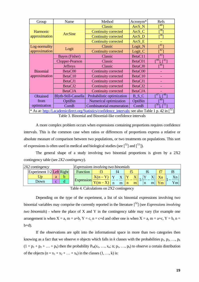
* As at: http://l.academicdirect.org/Statistics/confidence_intervals; see also Table 1 p. 42 in [52]Table 3. Binomial and Binomial-like confidence intervals

A more complex problem occurs when expressions containing proportions requires confidence

intervals. This is the common case when ratios or differences of proportions express a relative or

absolute measure of comparison between two populations, or two treatments on populations. This sort

of expressions is often used in medical and biological studies (see [52] and [53]).

The general shape of a study involving two binomial proportions is given by a 2X2

contingency table (see 2X2 contingency).

2X2 contingency Expressions involving two binomials Experiment 1\2 Left Right

Up a b Down c d

Function f3 f4 f5 f6 f7 f8

Expression )Xm(Y)Yn(X

−−

mX

nY−

mX

nY−

mX

nY/1 −

YmXn1−

YmXn

Table 4. Calculations on 2X2 contingency

Depending on the type of the experiment, a list of six binomial expressions involving two

binomial variables may comprise the currently reported in the literature [52] (see Expressions involving

two binomials) - where the place of X and Y in the contingency table may vary (for example one

arrangement is when X = a, m = a+b, Y = c, n = c+d and other one is when X = a, m = a+c, Y = b, n =

b+d).

If the observations are split into the informational space in more than two categories then

knowing as a fact that we observe n objects which falls in k classes with the probabilities p1, p2, …, pk

(1 = p1 + p2 + … + pk) then the probability PM(x1, …, xn; n; p1, …, pk) to observe a certain distribution

of the objects (n = x1 + x2 + … + xk) in the classes (1, …, k) is:

19

∏=

=k

1jj

xjiiM !xp!n)p;n;x(P j

We have many multinomial distributions when we discuss about the distribution of living

organisms in a certain area, for example distribution of bacteria species belonging on a class of bacteria

in a Petri plate after treatment with an antibiotic. Also for these cases we want to express with a certain

level of confidence, the effect of the treatment, for example.

Our knowledge about expressing confidence for expressions containing binomial variables can

be extent to cover trinomial (see Trinomial(6A,1B,1C) - distribution and 95% coverage confidence

interval) or multinomial variables as well [54].

0

12

34

56

7

01

23

45

67

8

0.000.05

0.10

0.15

0.20

0

12

34

56

7

01

23

45

67

8

0.000.05

0.10

0.15

0.20

Depicted: X (for A) - in depth axis, Y (for B) - left-to-right axis, P3(X,Y,Z) - vertical axis

Figure 4. Trinomial(6A,1B,1C) - distribution and 95% coverage confidence interval

Thus, any measurement on any three categories nominal scale may be seen as a series of two

binary measurements (fA="if A then 0 else 1"; fB="if B then 1 else 0") and this series of two

measurements is equivalent with a measurement on the three categories nominal scale meant to classify

in A, B, and C categories. Going further, {A, B, C} will be equivalent encoded in the informational

space by {10, 01, 00}. Similarly {0, 1, 2, …} can (and often is) equivalent encoded in the informational

space as (infinite) arrays (shown here in reverse order as we see the numbers in computer): 0→(000...),

1→(100...), 2→(010...), etc. For real values from [0,1) again providing the (infinite) series Σi≥1ai·2-i,

where ai∈{0,1} we gain a unique encoding for every number from [0,1) as a (infinite) series of binary

values starting with 0: 0.a1a2…; even further, the f(x)=1/(x-1) give us a unique correspondence between

[0,1) and [0,∞). This extent can be pushed forward to encode the sign too, and thus the existence of the

binary scale is enough to construct any real representation (and the computers do this).

Regarding the computation of the discriminating power of one scale relative to another, we take

this value from the total number of the distinct values encoded in the informational space, and Hartley's

entropy [55] sorts from this point of view of discriminating power the measurement scales.

Sampling

All procedures of quantitative analysis includes some common laboratory operations: taking of

20

the samples, drying, weighting and solvation [56]. Solvation is the only operation which is not always

necessary because exists some instrumental methods in which measurement is possible directly on the

sample [57]. Any experienced analyst performs these operations by giving them special attention, since

it is known that adequate preparation for measurement is as important as the measurement itself. A

sample must be representative for all components taking into account the extent to which these

components are included in the material to be analyzed. If the material is homogeneous, sampling is not

a problem. For heterogeneous materials special precautions are required to obtain a representative

sample. A sample sized laboratory can choose by chance or you can select a plan developed

statistically, which theoretically gives each component in the sample an equal chance of being detected

and analyzed.

Sampling from gaseous phase

There are 3 basic methods for collecting the gases. These are: the expansion of a container that

can then be discharged, washing and replacement of a liquid.

In all cases, you must know the volumes collecting vessels, temperature and pressure.

Typically, the collection vessels are made of glass and equipped with an inlet and an outlet which can

be opened and closed suitably. To eliminate contamination of samples, wash the outside of the

container with the gas to be sampled. Concept sampling device must allow this process to run

smoothly. Air is a complex mixture of different gases. Its actual composition is dependent on the

environment and on where the sample is taken. Currently, due to pollution, more efforts are directed to

study and monitor the air quality. The presence of air can cause various compounds that give specific

colour reactions, the amount of anions in the air (by reaction with a basic solution), or the amount of

cations in the air (the reaction with an acid solution).

In order to collect an air sample a simple collector is depicted below which also measure the

sample volume of air. In order to determine the concentration of anions in the air a possibility is by

titrating with a suitable base (NaOH), as the Figure 5 provides a schematic of an experimental

installation.

Working procedure can be imagined as follows:

÷ Measure the ambient temperature thermometer T;

÷ Measure the ambient pressure p with the barometer;

÷ Add the solution to capture the volume V of the air: 20 ml. solution of CaCl2 0.1M and 20 ml

solution of NaOH 0.1M;

÷ Fill with distilled water above the lower tube;

÷ Add a indicator for the presence of the pH = 7 (for instance bromothymol blue);

÷ Measure the diameter of the air inlet tube in the vicinity of the pressure gauge; let be d;

21

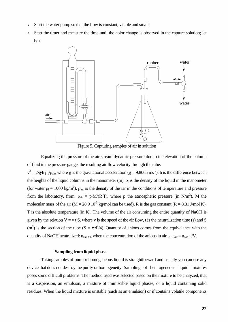
÷ Start the water pump so that the flow is constant, visible and small;

÷ Start the timer and measure the time until the color change is observed in the capture solution; let

be t.

air

rubber

water

water

Figure 5. Capturing samples of air in solution

Equalizing the pressure of the air stream dynamic pressure due to the elevation of the column

of fluid in the pressure gauge, the resulting air flow velocity through the tube:

v2 = 2·g·h·ρ1/ρair, where g is the gravitational acceleration (g = 9.8065 ms-2), h is the difference between

the heights of the liquid columns in the manometer (m), ρl is the density of the liquid in the manometer

(for water ρl = 1000 kg/m3), ρaer is the density of the iar in the conditions of temperature and pressure

from the laboratory, from: ρair = p·M/(R·T), where p the atmospheric pressure (in N/m2), M the

molecular mass of the air (M = 28.9·10-3 kg/mol can be used), R is the gas constant (R = 8.31 J/mol·K),

T is the absolute temperature (in K). The volume of the air consuming the entire quantity of NaOH is

given by the relation V = v·t·S, where v is the speed of the air flow, t is the neutralization time (s) and S

(m2) is the section of the tube (S = π·d2/4). Quantity of anions comes from the equivalence with the

quantity of NaOH neutralized: nNaOH, when the concentration of the anions in air is: cair = nNaOH/V.

Sampling from liquid phase

Taking samples of pure or homogeneous liquid is straightforward and usually you can use any

device that does not destroy the purity or homogeneity. Sampling of heterogeneous liquid mixtures

poses some difficult problems. The method used was selected based on the mixture to be analyzed, that

is a suspension, an emulsion, a mixture of immiscible liquid phases, or a liquid containing solid

residues. When the liquid mixture is unstable (such as an emulsion) or if contains volatile components

22

or if contains dissolved gases then additional difficulties arises. In general, aliquots are taken at random

from different depths and in all places in the liquid sample. They can be analyzed separately or can be

combined to give a sample composition, the static, representative of the original sample. Mixtures of

immiscible liquids are quite common in the art. The best known are mixtures of gasoline and oil +

water + water. Accidental oil spills are very unpleasant events ecosystems. For these mixtures phase

separation and then measuring the mixing ratio quantitative analysis of the separated fractions are

common methods in instrumental analysis of liquids. In addition to miscibility (in percent by weight

usually) a mixture of liquid is characterized by the distribution coefficient, which is defined for

distribution of a compound present in the mixture of the two phases, expressed as a weight ratio.

From a mixture of non-miscible liquids is possible to extract a solved component (Figure 6).

Figure 6. Extraction from a mixture of two non-miscible liquids

For two-component systems the separation of the two liquid phases is not total in general,

especially when one of the components is water and the other a liquid partially miscible with water. To

design an extraction mixture should be considered after evaluation of their miscibility in water.

Sampling from solid phase

Analysis of the solids can be made directly in the solid phase by means of emission or

absorption of radiation in the arc or flame (see [58]) or by moving the solid material in the form of a

solution by dissolution with or without changing the oxidation state of the constituent elements,

following the determination of the composition to be then make liquid phase by specific methods.

23

If the solid is homogeneous, any part can be selected as representative. For a heterogeneous

solid a plan should be prepared to reach all sections of solid statistical sampling. Sampling can be done

manually or mechanically, when the material to be analyzed has a large table (see Figure 7).

Figure 7. Devices for reducing sample size: crusher, transversal and parallel cutters

It is not always possible to obtain statistically, a representative sample. For example, it is

obviously a difficult task to determine the surface composition of. Starting with a limited amount of

rock and dust sampling has been based in part on the size of the particles and partly on their physical

condition. Particle size is an important parameter in the sampling of a solid, because the composition of

particles of different sizes can vary. In general, higher conversion of a sample in a sample of suitable

size for analysis requires, first, the reduction of the sample to a uniform particle size and second, the

reduction in mass of the sample. A uniform particle size is obtained by passing the sample through

crushers, pulverizers, mills or mortars. It can also be used for screening granular or metal filing.

Whatever the method chosen, it is necessary to ensure that these operations will not contaminate the

sample.

Drying

After obtaining the corresponding sample, further analysis will be decided if will be conducted

with whether the sample as such or after it has been dried. Most samples contain varying amounts of

water due to the fact that the sample is hygroscopic or water is absorbed at the surface. The drying

operation is typically by heating in an oven, a muffle furnace or combustion Bunsen or Meeker lamps.

Since heat is used for drying, it is possible that the sample drying her attempt to decompose or

lose volatiles. Both cases must be considered in making a correct analysis. After the sample was dried,

will be typically weight. To do this, use the scales. Balances are mass measuring instruments, but there

are several types: technical balance (with precision of grams used for weights of substances whose

mass exceeding 1 kg), pharmaceutical balance (precision of 1 to 10 mg used for weights of substances

whose mass exceeds 100g), analytical balance (precision 0.1 mg used for weighing substances whose

weight is below 100g), electronic scales (table-recording changes over time) [1].

24

Figure 8. Devices for drying the samples

Dissolving

After weighing the sample, the next step may be dissolving. If the sample is soluble in water,

there is no problem of the dissolution, though sometimes slow sample may hydrolyze in water to form

insoluble compounds. Organic materials are commonly dissolved in organic solvents or in mixtures of

organic solvents and water. There are a variety of chemical processes and tools that require a specific

solvent composition. In other cases it not necessary the step of dissolution. Thus, the sample is excited

in the arc or spark and then analyzes the resulting radiant energy can be used directly in a liquid or solid

sample. If required to be considered organic part of the mixture of sample taken, then you must use

specific organic solvents and organic chemistry technologies. For inorganic samples, the most frequent

in the industry, the sample is dissolved in an acid or a flux melts. When using acids, it is important to

know the chemical properties of the sample, if necessary oxidizing or non-oxidizing acid, if the process

applied must comply with restrictions on the type of anion in solution, and if after dissolution should be

deleted or not excess the acid.

Specific situations: H2SO4 should not be used for samples containing Ba (BaSO4 is a white

precipitate which is insoluble); HCl should not be used for samples with Ag or Ag salts (AgCl is a

white precipitate which is insoluble). The selection of the particular acid to be used for the dissolution

is carried out on the basis of their chemical properties, they are oxidising or non-oxidising. Non-

oxidising acids used are HCl, diluted H2SO4, and diluted HClO4. Oxidizing acids are: HNO3, H2SO4

and hot concentrated HClO4. The dissolution of the metal by means of non-oxidising acids is based on

the ability of metals to replace hydrogen. In this case, you must take into account the chemical activity

series of metals

Li, Ca, K, Ba, Na, Mg, Al, Zn, Fe, Cd, Co, Ni, Sn, Pb, H, Cu, Ag, Hg, Au

The stronger oxidizing conditions are obtained with the use of hot and concentrated HClO4,

usual dissolving all metals. Often advantages are gained from the use of combination of acids. The

most familiar is aqua regia (1:3 of HNO3:HCl) from which HNO3 is an oxidant and HCl have

complexing properties and provide strong acidity. Note that the solubility of many metal ions is

maintained only in the presence of complexing agents. Hydrogen fluoride (HF), although a weak acid

25

and non-oxidizing, provides rapid decomposition of silicate samples with SIF4 obtaining. It have a

higher complexing action than hydrochloric acid (HCl). HNO3+HClO4 mixture has a much more

vigorous action to dissolve, but require more careful handling because it can cause explosions.

Fluxing is more effective than treatment with acid for two reasons. First, due to the higher

temperature necessary for melting (from 300 °C to 1000 °C) is the reaction processes to be carried out

more easily. The second advantage is that if fluxes in contact with the sample there is a greater amount

of reactive, making the reaction is faster and more shifted towards the formation of products.

Sampling distribution and distribution analysis

Systematic repeated measurements of a certain characteristic from a population lead to the

concept of distribution from sampling. Let be a statistic in a population subject to measurement. The

sampling distribution is the distribution of that statistic, considered as a random variable, when derived

from a random sample of fixed size n. It may be considered as the distribution of the statistic for all

possible samples from the same population of a given size. The sampling distribution depends on the

underlying distribution of the population, the statistic being considered, the sampling procedure

employed, and the sample size used. There is often considerable interest in whether the sampling

distribution can be approximated by an asymptotic distribution, which corresponds to the limiting case

as n → ∞.

There are a series of known (theoretical) distributions and when repeated sampling is involved,

the expectance is that data to fit to a known distribution. Usually this stage supposes to assess the fit of

the data to one or more alternatives and involves using of a series of statistics measuring the agreement

(see [59], [60], [61] and [62] for further details).

[79], [80] and [81].

When exists a doubt about the celerity with which the data was collected, a useful test is the

Benford test [63].

When measurements are more likely opinions recorded on ordinal scales (see for instance [64]

and [65]) then testing for a binomial proportion may require optimization of the distribution parameters,

as were conducted in [66] and [67].

When contingencies are behind the observation, then using of the Chi-Squared statistic (see

[68]) is a good alternative, as is exemplified in [69], and in other cases design of the experiment (see

[70], [71], [72] and [73]) is the preliminary step (the factor analysis may be the second one, as

exemplified in [74] and [75]) through the characterization of the population, as is exemplified in [76],

[77], [78],

In some cases, the phenomena lead to the distribution (see [82], [83] for details). In other cases,

recording of the observed distribution may be enough to characterize the phenomena (as is exemplified

in [84]) while in other cases may have as outcome a statistic (see [85]).

26

The most convenient case is when enough data for obtaining the distribution of the population

are available (see typical cases in: [86], [87], [88], [89], [90], [91]) but also from incomplete data some

information may be successfully extracted (see [92], [93], [94] and [95]).

137]).

.

Rarefaction method may help to reconstruct the sampling distribution (see [96] for details) and

smoothing may help to indicate the general tendency (see [97], [98], [99], and [100]).

Association and regression analysis

The expected result when an association between paired observations is under investigation is

the linearity (see [101], [102], [103], [104] and [105]; see as examples of linear regression analysis: [106],

[107], [108], [109], [110], [111], [112], [113], [114], [115], [116], [117], [118], [119], [120], [121], [122], [123], [124],

[125], [126], [127], [128], [129], and [130]), but other models may occurs too (see [131], [132], [133], [134],

[135], [136] and [

A difficult task is to assess the quality of the regression model (see [138], [139], [140], [141], [142],

[143], [144], [145], [146], [147] and [148] for details)

27

Study of the diffusion in gaseous state and molecular speeds

Introduction

Were established following inequalities (see Ex.23 in [5]; see also [149]), in which the energy at

mode is smaller than the energy of the molecules with the mode speed, which is smaller than the

energy of the molecules with average speed, which is smaller than the energy of the molecules with the

speed equal with average of squared speed:

Tk2

2Jˆ B⋅−

=ε ≤ Tk2

1J2sm

B

2

⋅−

= ≤ Tk2J

21J

2sm

B

22

⋅⎟⎠

⎞⎜⎝

⎛⎟⎠⎞

⎜⎝⎛Γ⎟

⎠⎞

⎜⎝⎛ +

Γ= ≤ Tk2J

B⋅=ε

Expressing the relationships on R·T (R = kB·NA; m·NA = M):

( ) JMs

)2/J()2/)1J((2Ms

1JMs

2JMsRT

2

2

2s

2s

2ˆ εε =

Γ+Γ=

−=

−=

For two gases at the same temperature the kB·T term is the same, allowing the obtaining of a

relationship between the masses and the speeds. This law can be easily verified experimentally with a

simple experiment of diffusion in gaseous state. Are phrased thus the hypothesis that the diffusion

speed is proportional with the speed of the molecules. For the speed of the molecules we have, as was

shown above, more than one statistic: real speeds (when the number of the energy components J, is

always 3) and virtual speeds (when the number of the energy components depends on the structure of

the molecules).

Thus, are opened the problem to identify which is the number of the energy components

(labeled with J) which are used by the molecules in the diffusion process, and here the effect can be

with the models expressed from virtual (labeled as s), or real (labeled as v) speeds, which of the

statistics, namely the mean (labeled with an over-bar) or the mode (labeled with an hat) as well as

which of the physical quantity: speed (labeled with s) or energy (labeled with ε, ε ~ s2) correspond to

the observable (formation of the NH4Cl ring in the experiment which will be conducted).

Purpose

Establishing by experimental path the diffusion speeds, and on this way, of the model linking

the diffusion speeds with the molecular speeds (seen as molecular statistics) derived from molecular

kinetic theory, leading to the obtaining of the diffusion coefficients.

Material and method

It will be studied the reaction in gaseous state between ammonia and hydrochloric acid. Both

these substances are solved in water, and thus a series chemical reactions can be written, as are given in

the next table (see Table 1).

28

No Equilibrium chemical reactionR1 HCl + H2O ↔ Cl- + H3O+

R2 NH3 + H2O ↔ NH4+ + HO-

R3 NH3 + HCl ↔ NH4Cl R4 NH4

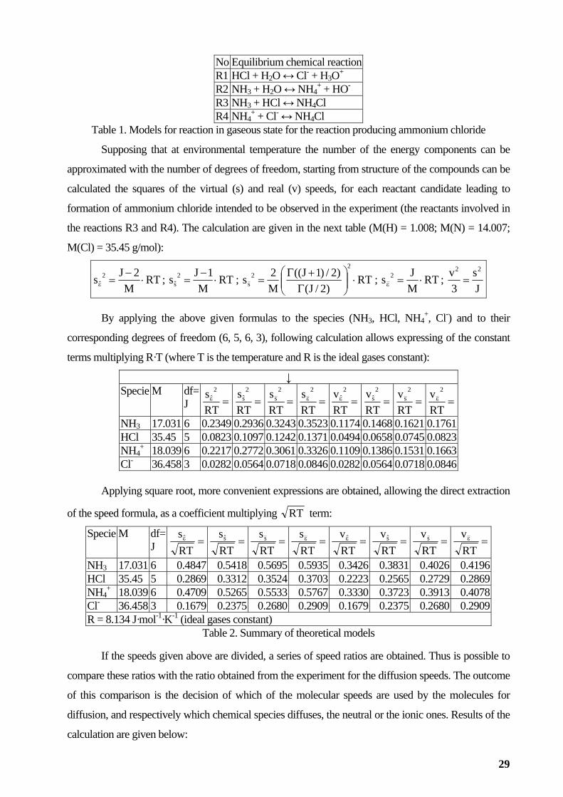
+ + Cl- ↔ NH4Cl Table 1. Models for reaction in gaseous state for the reaction producing ammonium chloride

Supposing that at environmental temperature the number of the energy components can be

approximated with the number of degrees of freedom, starting from structure of the compounds can be

calculated the squares of the virtual (s) and real (v) speeds, for each reactant candidate leading to

formation of ammonium chloride intended to be observed in the experiment (the reactants involved in

the reactions R3 and R4). The calculation are given in the next table (M(H) = 1.008; M(N) = 14.007;

M(Cl) = 35.45 g/mol):

RTM

2Js 2ˆ ⋅

−=ε ; RT

M1Js 2

s ⋅−

= ; RT)2/J(

)2/)1J((M2s

22

s ⋅⎟⎟⎠

⎞⎜⎜⎝

⎛Γ+Γ

= ; RTMJs 2 ⋅=ε ;

Js

3v 22

=

By applying the above given formulas to the species (NH3, HCl, NH4

+, Cl-) and to their

corresponding degrees of freedom (6, 5, 6, 3), following calculation allows expressing of the constant

terms multiplying R·T (where T is the temperature and R is the ideal gases constant):

↓ Specie M df=

J =ε

RTs 2

ˆ =RTs 2

s =RTs 2

s =ε

RTs 2

=ε

RTv 2

ˆ =RTv 2

s =RTv 2

s =ε

RTv 2

NH3 17.031 6 0.2349 0.2936 0.3243 0.3523 0.1174 0.1468 0.1621 0.1761 HCl 35.45 5 0.0823 0.1097 0.1242 0.1371 0.0494 0.0658 0.0745 0.0823 NH4

+ 18.039 6 0.2217 0.2772 0.3061 0.3326 0.1109 0.1386 0.1531 0.1663 Cl- 36.458 3 0.0282 0.0564 0.0718 0.0846 0.0282 0.0564 0.0718 0.0846

Applying square root, more convenient expressions are obtained, allowing the direct extraction

of the speed formula, as a coefficient multiplying RT term:

Specie M df=J =ε

RTsˆ =

RTss =

RTss =ε

RTs

=ε

RTvˆ =

RTvs =

RTvs =ε

RTv

NH3 17.031 6 0.4847 0.5418 0.5695 0.5935 0.3426 0.3831 0.4026 0.4196HCl 35.45 5 0.2869 0.3312 0.3524 0.3703 0.2223 0.2565 0.2729 0.2869NH4

+ 18.039 6 0.4709 0.5265 0.5533 0.5767 0.3330 0.3723 0.3913 0.4078Cl- 36.458 3 0.1679 0.2375 0.2680 0.2909 0.1679 0.2375 0.2680 0.2909R = 8.134 J·mol-1·K-1 (ideal gases constant)

Table 2. Summary of theoretical models

If the speeds given above are divided, a series of speed ratios are obtained. Thus is possible to

compare these ratios with the ratio obtained from the experiment for the diffusion speeds. The outcome

of this comparison is the decision of which of the molecular speeds are used by the molecules for

diffusion, and respectively which chemical species diffuses, the neutral or the ionic ones. Results of the

calculation are given below:

29

Case Speeds ratio (vA/vB) Observation range R3 (A=NH3, B=HCl), mode energy (ε ), virtual speed (s) ˆ 1.689 R3 (A=NH3, B=HCl), mode speed (s ), virtual speed (s) ˆ 1.636 R3 (A=NH3, B=HCl), average speed ( s ), virtual speed (s) 1.616 R3 (A=NH3, B=HCl), average energy ( ε ), virtual speed (s) 1.603 R3 (A=NH3, B=HCl), mode energy (ε ), real speed (v) ˆ 1.542 R3 (A=NH3, B=HCl), mode speed (s ), real speed (v) ˆ 1.494 R3 (A=NH3, B=HCl), average speed ( s ), real speed (v) 1.475 R3 (A=NH4

+, B=Cl-), average energy ( ε ), real speed (v) 1.463 R4 (A=NH4

+, B=Cl-), mode energy (ε ), virtual speed (s) ˆ 2.804 max (vB/(vA+vB) ≈ 0.26)R4 (A=NH4

+, B=Cl-), mode speed (s ), virtual speed (s) ˆ 2.217 R4 (A=NH4

+, B=Cl-), average speed ( s ), virtual speed (s) 2.065 R4 (A=NH4

+, B=Cl-), average energy ( ε ), virtual speed (s) 1.983 R4 (A=NH4

+, B=Cl-), mode energy (ε ), real speed (v) ˆ 1.983 R4 (A=NH4

+, B=Cl-), mode speed (s ), real speed (v) ˆ 1.568 R4 (A=NH4

+, B=Cl-), average speed ( s ), real speed (v) 1.460 R4 (A=NH4

+, B=Cl-), average energy ( ε ), real speed (v) 1.402 min (vB/(vA+vB) ≈ 0.42)

Experimental apparatus

For the experiment of diffusion in gaseous state of the chemical species involved in formation

of the ammonium chloride (HCl, Cl-, NH3, NH4+) are required a glass tube of (at least) 1m length and a

diameter of about 2 cm. The tube must be dry. Are also required two rubber stoppers, two cotton pads,

a horizontal fixing frame of the glass tube, and a timer for measuring a straight edge distance (see Fig.

E5).

Fig. E5. Experimental apparatus for the study of diffusion in gaseous state

Working procedure

Assemble the experimental apparatus as shown in Fig. E6

Glass tube

Clamp

Sub-frame

Clamp Glass tube Rubber stopper

Fig. E6. The experimental setup for studying the gaseous diffusion

30

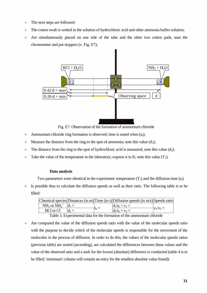
÷ The next steps are followed:

÷ The cotton swab is wetted in the solution of hydrochloric acid and other ammonia buffer solution;

÷ Are simultaneously placed on one side of the tube and the other two cotton pads, start the

chronometer and put stoppers (v. Fig. E7);

Fig. E7. Observation of the formation of ammonium chloride

HCl + H2O NH3 + H2O

÷ Ammonium chloride ring formation is observed; time is noted when (t0);

÷ Measure the distance from the ring to the spot of ammonia; note this value (d1);

÷ The distance from the ring to the spot of hydrochloric acid is measured; note this value (d2);

÷ Take the value of the temperature in the laboratory; express it in K; note this value (T1);

Data analysis

Two parameters were identical in the experiment: temperature (T1) and the diffusion time (t0).

÷ Is possible thus to calculate the diffusion speeds as well as their ratio. The following table is to be

filled:

Chemical species Distances (in m) Time (in s) Diffusion speeds (in m/s) Speeds ratioNH3 or NH4

+ d1 = d1/t0 = v1 = HCl or Cl- d2 = t0 = d2/t0 = v2 = v1/v2 =

Table 3. Experimental data for the formation of the ammonium chloride

÷ Are compared the value of the diffusion speeds ratio with the value of the molecular speeds ratio

with the purpose to decide which of the molecular speeds is responsible for the movement of the

molecules in the process of diffusion. In order to do this, the values of the molecular speeds ratios

(previous table) are sorted (ascending), are calculated the differences between these values and the

value of the observed ratio and a seek for the lowest (absolute) difference is conducted (table 4 is to

be filled; 'minimum' column will contain an entry for the smallest absolute value found):

Observing space 0.42·d = max

d 0.26·d = min

31

Case B

A

vv

2

1

B

A

vv

vv

− 2

1

B

A

vv

vv

− =minim

R4 (A=NH4+, B=Cl-), average energy ( ε ), real speed (v) 1.402 ?

R4 (A=NH4+, B=Cl-), average speed ( s ), real speed (v) 1.460 ?

R3 (A=NH4+, B=Cl-), average energy ( ε ), real speed (v) 1.463 ?

R3 (A=NH3, B=HCl), average speed ( s ), real speed (v) 1.475 ? R3 (A=NH3, B=HCl), mode speed ( ), real speed (v) s 1.494 ? R3 (A=NH3, B=HCl), mode energy ( ε ), real speed (v) 1.542 ? R4 (A=NH4

+, B=Cl-), mode speed ( s ), real speed (v) 1.568 ? R3 (A=NH3, B=HCl), average energy ( ε ), virtual speed (s) 1.603 ? R3 (A=NH3, B=HCl), average speed ( s ), virtual speed (s) 1.616 ? R3 (A=NH3, B=HCl), mode speed ( ), virtual speed (s) s 1.636 ? R3 (A=NH3, B=HCl), mode energy ( ε ), virtual speed (s) 1.689 ? R4 (A=NH4

+, B=Cl-), average energy ( ε ), virtual speed (s) 1.983 ? R4 (A=NH4

+, B=Cl-), mode energy ( ε ), real speed (v) 1.983 ? R4 (A=NH4

+, B=Cl-), average speed ( s ), virtual speed (s) 2.065 ? R4 (A=NH4

+, B=Cl-), mode speed ( s ), virtual speed (s) 2.217 ? R4 (A=NH4

+, B=Cl-), mode energy ( ε ), virtual speed (s) 2.804 ? Table 4. Measuring agreement between the observation and the models- models sorted by speeds ratio

÷ Is identified the lowest absolute difference and thus are identified the chemical species which

diffuses in gaseous state as well as the link between molecular speeds and diffusion speeds.

÷ The relations which characterize the model are written. These include the reaction of the formation

of the ammonium chloride (R3 or R4), determinant factors in diffusion (energy or speed; real or

virtual speeds; see also [150] and [151]) and expressions of the molecular speeds for the identified

model;

÷ The coefficients of diffusion are calculated as ratios between diffusion speeds and molecular

speeds: c1 = c(NH3/NH4+) = v1/vA; c2 = c(HCl/Cl-) = v2/vB, where vA and vB are the molecular

speeds and their values depends on the obtained model; for instance when A = "NH4+", the best

model agreeing with the experimental data is based on average energy (ε ) and real speed (v), then

vA = )NH(v 4+

ε = 0.4196· RT (this is an example of calculation only; see Table 2);

÷ Following table should be filled:

Equation of the chemical reaction F1: energy or speed F2: real or virtual Coefficients of diffusionc1 = c2 =

Table 5. Diffusion coefficients and the kinetic model for diffusion Further reading

Systems of particles and the rarefaction method

For a system S with N molecules having a number M of distinct energy states (let be N1

molecules in the energy state ε1, ..., NM in the energy state εM; then N = Σ1≤i≤MNi). Sorting the energy

states (ε1 < ... < εM) does not affect the observation. Observing n out of N molecules exiting in the

32

system, a question is raised: how many molecules should be observed (let's assume that the observation

is simultaneous) such that the entire diversity of energy states to be captured?

Firstly, capturing of the whole diversity (M) is a matter of chance. Second, is obviously that is

necessary at least n ≥ M. Third, an isolated experiment affected or not by chance, will not characterize

the system, while a repeating of it many times will assure that the (obtained) mean will be a sufficiency

statistic [152] (see also [68]).

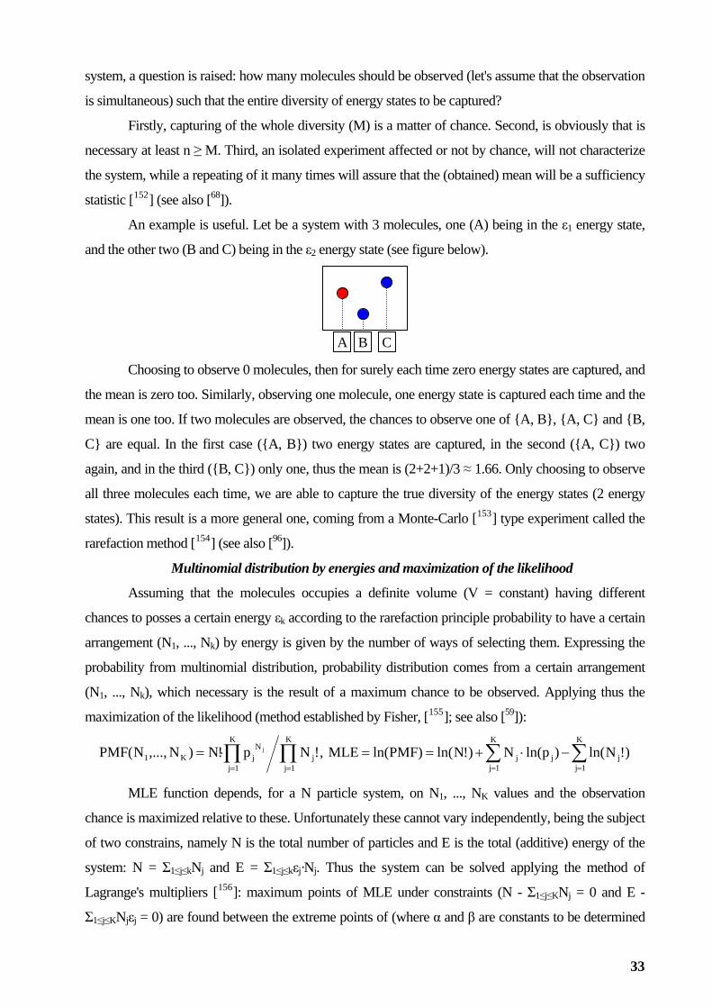
An example is useful. Let be a system with 3 molecules, one (A) being in the ε1 energy state,

and the other two (B and C) being in the ε2 energy state (see figure below).

A B C Choosing to observe 0 molecules, then for surely each time zero energy states are captured, and

the mean is zero too. Similarly, observing one molecule, one energy state is captured each time and the

mean is one too. If two molecules are observed, the chances to observe one of {A, B}, {A, C} and {B,

C} are equal. In the first case ({A, B}) two energy states are captured, in the second ({A, C}) two

again, and in the third ({B, C}) only one, thus the mean is (2+2+1)/3 ≈ 1.66. Only choosing to observe

all three molecules each time, we are able to capture the true diversity of the energy states (2 energy

states). This result is a more general one, coming from a Monte-Carlo [153] type experiment called the

rarefaction method [154] (see also [96]).

Multinomial distribution by energies and maximization of the likelihood

Assuming that the molecules occupies a definite volume (V = constant) having different

chances to posses a certain energy εk according to the rarefaction principle probability to have a certain

arrangement (N1, ..., Nk) by energy is given by the number of ways of selecting them. Expressing the

probability from multinomial distribution, probability distribution comes from a certain arrangement

(N1, ..., Nk), which necessary is the result of a maximum chance to be observed. Applying thus the

maximization of the likelihood (method established by Fisher, [155]; see also [59]):

∏∏==

⋅=K

1jj

K

1j

NjK1 !Np!N)N,...,N(PMF j , ∑∑

==

−⋅+==K

1jj

K

1jjj )!Nln()pln(N)!Nln()PMFln(MLE

MLE function depends, for a N particle system, on N1, ..., NK values and the observation

chance is maximized relative to these. Unfortunately these cannot vary independently, being the subject

of two constrains, namely N is the total number of particles and E is the total (additive) energy of the

system: N = Σ1≤j≤kNj and E = Σ1≤j≤kεj·Nj. Thus the system can be solved applying the method of

Lagrange's multipliers [156]: maximum points of MLE under constraints (N - Σ1≤j≤KNj = 0 and E -

Σ1≤j≤KNjεj = 0) are found between the extreme points of (where α and β are constants to be determined

33

reducing the number of variables):

⎟⎟⎠

⎞⎜⎜⎝

⎛ε⋅−β+⎟⎟

⎠

⎞⎜⎜⎝

⎛−α+−⋅+= ∑∑∑∑

====

K

1jjj

K

1jj

K

1jj

K

1jjjk1 NENN)!Nln()pln(N)!Nln(l)N,...,N(1MLE

Derivative of MLE1 relative to a variable (observable) Ni is:

( ) ( ) ( ) )NE(N

)NN(N

!NlnN

plnN

!NlnN

0K

1jjj

i

K

1jj

i

K

1jj

i

Nj

K

1jii

j ∑∑∑∑====

⋅ε−β∂∂

+−α∂∂

+∂∂

−∂∂

+∂∂

≡

and are fulfilled simultaneously for each i. It result thus a relation between Ni, their appearance

probability pi and their energy εi:

)N(N

)N(N

)!Nln(N

)pln(NN

0 iii

ii

ii

iii

⋅εβ∂∂

−α∂∂

−∂∂

−∂∂

= → iiii

)pln()!Nln(N

βε−α−=∂∂

where ∂(ln(·))/∂(·)=Ψ(·) is digamma function, α and β are the same for any i (being thus statistics of the

distribution of the molecules by energy). Equation doesn't have an analytical solution for any x (Ni).

Digamma function can be expressed using [157]:

∑=

+γ−=+ΨiN

1ji j1)1N( , or ( ))Nln()1N(lim0 iiNi

−+Ψ=∞→

where γ = -Ψ(1) is the Euler's constant [158]. For large numbers (Ni >> 1) is possible to approximate to

obtain a relationship between energy and the number of particles, Boltzmann [159] arriving to (solution

retrieved using Stirling's approximation [160]):

iii )pln()Nln( βε−α−= → iepN iiβε−α−=

It should be noted that the previous formula is only an approximate one (see [82] and [83]).

Distribution by speed for an arbitrary number of energy components

By skipping some steps, it can be shown that the previous given formula may provide a

distribution of the speeds for an energy component: 22xaea)x(f π−⋅= , where )pV2/(mNa2 π=

Assuming that the kinetic energy have J components (ε = ε1 + ε2 + ... + εJ) and for each

component a virtual (s) speed may be expressed along it (εj = m·sj2/2), the value of the probability that a

molecule to have s1, s2, ..., sJ as the components of the virtual speed is given by dP =

f(s1)f(s2)...f(sJ)ds1ds2...dsJ and the mean of speed and the mean of square speed are given by the

relations:

∫ ∫ ∫ ∏∑∞

∞−

∞

∞−

∞

∞− ==

⋅= J21

J

1jj

J

1j

2j ds...dsds)s(fs...)s(M ; ∫ ∫ ∫ ∏∑

∞

∞−

∞

∞−

∞

∞− ==

⋅⎟⎟⎠

⎞⎜⎜⎝

⎛= J21

J

1jj

J

1j

2j

2 ds...dsds)s(fs...)s(M

It may be checked using substitution method that (the energy equipartition on its components):

34

pV2mN

2J

21

2J

a2J

21

2J

)s(M2/1

⎟⎠⎞

⎜⎝⎛Γ

⎟⎠⎞

⎜⎝⎛ +Γ

=π⎟⎠⎞

⎜⎝⎛Γ

⎟⎠⎞

⎜⎝⎛ +Γ

= ; mNpVJ

a2J

12J

)s(M2

2 ⋅=π⎟⎠⎞

⎜⎝⎛Γ

⎟⎠⎞

⎜⎝⎛ +Γ

= ; pV2J

2)s(MmNE

2

⋅=⋅

⋅=

Ideal gas law and the relation between the temperature and the molecular speed

Synthesising a series of obtained results, were established that:

mNpV)v(M

31 2 = ,

mNpV)v(M

82 =

π , mNpV)s(M

J1 2 = , ( )

( ) mNpV)s(M

212J22J 2

2

=⎟⎟⎠

⎞⎜⎜⎝

⎛

+ΓΓ

where v is the real speed of the molecules, and s is the virtual speed of the molecules.

Experimentally the relation was checked and the demonstrative experiment were possible with

the help of the thermometer assuring (keeping T = constant) the thermal equilibrium or tracing (when T

varies) the energy transfer between systems and environment. By using the Kelvin scale for

temperature, was shown that (where R, NA and kB are experimental constants: R = 8.3144621(75) J·K-

1·mol-1, ideal gas constant; NA = 6.02214129(27)·1023 mol-1, Avogadro's number; kB =

1.3806488(13)·10-23 J·K-1, Boltzmann's constant): pV = NRT/NA = NkBT.

A simple identification between terms can be done, taking into account that m = M/NA where

M have the meaning of molar mass (contrasting with M(x) used here for mean of x), when it results:

MRT)v(M

31 2 = ,

MRT)v(M

82 =

π , MRT)s(M

J1 2 = , ( )

( ) MRT)s(M

212J22J 2

2

=⎟⎟⎠

⎞⎜⎜⎝

⎛

+ΓΓ

35

Obtaining of the oxygen: study of the gases laws

Introduction

Gaseous state is characterized by an internal energy from which most transforming part is

kinetic energy. Very often, for small enough pressures and for high enough temperatures the gas is

approximated as being an ideal one, using the relationship between its state parameters with:

p·V = n·R·T R = 8.314 J/mol/K→ p·M = ρ·R·T (Ideal)

A more exact treatment of the gaseous state is by involving the thermodynamic functions [161].

Anyway, obviously 'small enough' (for pressure) and 'high enough' (for temperature) depends on the

chemical composition of the gas. For instance at 101325 Pa (1 atm) and 298 K (25 °C) O2 is in gaseous

state, S8 is in solid state while H2O is in liquid state. At a given pressure, as temperature become much

higher than the vaporization temperature (of passing into gaseous state) with (about) the same the

approximating error when is considered an ideal one it becomes smaller.

Often used approximations for the behaviour of a real gas are actually corrections applied to the

ideal gas law by analytical formulas named virial, and expressed as is given in eq.1, where B = B(T), C

= C(T) are functions of temperature and Vm = V/n is the molar volume. Since higher order terms

multiplying the inverse of the molar volume (C, ...) contributes increasingly less at the value (of the

sum of), often is used the first approximation of the virial equation (eq.2).

The disadvantage of the virial equations is that the values of coefficients depend on the gas

composition. To have an image of expressing the virial equations, please look at the virial equation for

hydrogen (eq.3).

...)VC

VB1(

VRTp 2

mmm

+++= )VB1(

VRTp

mm

+= ∑=

−

⎟⎠⎞

⎜⎝⎛ −=

n

1i

1i0

i 1TTaB

a1 = 15.4 a2 = -9.00 a3 = -0.21

H2: n = 3, T0 = 298.15 K

(eq.1) (eq.2) (eq.3) Other approximations are given by the relations implying the critical values for the pressure

and temperature. Critical point, characterized by critical pressure, critical temperature and critical molar

volume is the point from which ('from which' is regarding the temperature and the pressure) in general,

doesn't exist any more phase frontier (in general; in particular, here is about the frontier between liquid

and gaseous state). For instance, for water the phase frontier between liquid and gaseous states

disappears when T ≥ TC = 647 K (374 °C) and p ≥ pC = 22.064 MPa (218 atm).

Anyway, there are many equations proposed to be used being in use today for the

approximating of the real gases evolution. A part of these equations which are most often used are

given in the next, for the purpose to be used in calculations as a part of the laboratory activity:

36

÷ Van der Waals [162] model:

2mm Va

bVRTp −−

= C

2C

2

pTR

6427a = ,

C

C

pRT

81b =

→ 0ab/pMab/)pbRT(Mb/M 3223 =−+ρ+ρ−ρ

(Waals)

÷ Abel-Noble [163] model:

bVRTpm −

=C

C

pRT

81b =

→ b)pM/()RT(1 +=ρ−

(Abel-Noble)

÷ Redlich-Kwong [164] model:

5.0mmm T)bV(V

abV

RTp+

−−

= C

5.2C

2

pTR

400171a = ,

C

C

pRT

30026b =

→ ρ 0ab/TpMab/MRTab/)abpTRbT(M 5.0325.125.05.123 =−ρ+−+ρ+

(Redlich-Kwong)

÷ Modified Berthelot [165] model:

)aba1(VRTp

m

−+=C

C

T/Tp/p

1289a = , 2

C )T/T(6b =

→ )aba1(RTpM ρ + −= (Berthelot)

÷ Clausius [166] model:

2mm )cV(Ta

bVRTp

+−

−=

C

3C

2

pTR

6427a = ,

C

CC p4

RTVb −= , CC

C Vp

RT83c −= (Clausius)

→ 0pTbccRTab

pTMpTbccRTab

)pc2pbRT(TMpTbccRTab

)apTcpTbc2cRT2(M222

3

222

2

222

2223 =

++−

+++

ρ+++

−−+ρ+ρ

−

÷ hl [167] model: Wo

3m

2mmm VT

c)bV(VT

aRT+

−bVp −

−= 2

CCC VTp6a = , 4

Vb C= , 3C

2CC VTp4c = (Wohl)

→ 0bc

MpTbc

)RTpb(MTbc

aTMbM 42322

234 =++

ρ−ρ+ρ−ρ

The disa tage of the state equations (given above) for the real gase consists in the fact that

e constants implied in the models having an expression depending on the critical parameters can be

hus being useful the constants of the models for it (for oxygen).

dvan s

th

obtained only for pure gases, and thus for mixtures the values of the constants implied in models should

be experimentally determined. For instance for air the values of the Van der Waals model constants are

a = 0.1358 and b = 3.64·10-5.

In the laboratory it is easily to obtain pure oxygen through thermal decomposition of the

oxygen rich containing salts, t

37

Purpose

The experiment will be conducted operationalizing the mass conservation principle and thus

comparing of the experimental results with the ones coming from the applying of the gases equations

of state. It will be studied the oxygen produced from the decomposition of a potassium salt.

Material and method

In the presence of a catalyst (here MnO2 will be used) occurs relatively fast the thermal

decomposition of the potassium chlorate in potassium chloride when oxygen are released, as is given

by the equation of the chemical reaction:

KClO3 → KCl + 3/2O2 (MnO2, t°C)

For the values of the critical constants, ref. [168] should be used. Here is a series of values: Substance TC (K) pC (MPa) VC,m (cm3/mol)Oxygen (O2) 154.59 5.043 73 Ozone (O3) 261.1 5.57 89 Nitrogen (N2) 126.21 3.39 90 Water (H2O) 647.14 22.06 56 Carbon dioxide (CO2) 304.3 7.375 94 Sulphur dioxide (SO2) 430.64 7.884 122 Argon (Ar) 150.87 4.898 75 Hydrogen (H2) 32.97 1.293 65 Helium (He) 5.19 0.227 57 Carbon monoxide (CO) 132.86 3.494 93 Methane (CH4) 190.56 4.599 98.6 Octane (C8H18) 568.7 2.49 492

For the values of the virial coefficients a call for a catalogue of physical and chemical constants

can be pursued, as is CRC [169]. Here a list of values is given (for p·Vm2 = RT(Vm + B); B = Σiai(T0·T-1

-1)i-1, T0 = 273.15 K): Substance Coefficients Oxygen (O2) a1= -16; a2 = -62; a3 = -8; a4 = -3 Carbon dioxide (CO2) a1 = -127; a2 = -288; a3 = -118 Carbon monoxide (CO) a1 = -9; a2 = -58; a3 = -18 Methane (CH4) a1 = -43; a2 = -114; a3 = -19; a4 = -7 Sulphur dioxide (SO2) a1 = -430; a2 = -1193; a3 = -1029 Water (H2O) a1 = -1158; a2 = -5157; a3 = -10301; a4 = -10597; a5 = -4415 Helium (He) a1 = 12.44; a2 = -1.25 Ammonia (NH3) a1 = -271; a2 = -1022; a3 = -2715; a4 = -4189 Argon (Ar) a1 = -16; a2 = -60; a3 = -9.7; a4 = -1.5

For the general form of the virial model, Wagner & collaborators [170] determined the

expressions of the first and of the second virial coefficient for oxygen, the result being given in the next

table.

p = (1 + B·Vm + C·Vm2)·Vm·R·T

B = b1 + b2·T-0.25 + b3·T-3.5 + b4·T-4.5 + b5·T-5.5

C = c1·T-0.25 + c2·T-6 + c3·T-6.75 (Wagner)

For T in K, B in dm3/mol and C in (dm3/mol)2 : b1 = 0.143389 c1 = 0.451336·10-2

b2 = -0.629863 c2 = 0.987169·1011

b3 = -0.577814·107 c3 = -0.364928·1013

Oxygen

38

b4 = 0.695858·109 b5 = -0.246023·10 11

ig. 1): working table, a beaker or a flask of any

for the gas burner, supporting frame and fixing clamps for

barometer, a thermometer and a graduated cylinder, all being part of the

equipment of the laboratory where ex

To simplify the processing of data were calculated the Van der Waals coefficients for oxygen

(a = 1.382·10-5 dm6/mol2 and b = 0.0319 dm3/mol) and ozone (a = 3.570·10-5 and b = 0.0487).

Experimental apparatus

To conduct the experiment are necessary (see F

type, a test tube, a large round bottom flask (with at least two necks), three perforated rubber stoppers

and traversed with glass tubes (one with a long tube), two rubber hoses, support for the large round

bottom flask, gas burner, elevating system

sustaining the test tube (last ones not depicted in Fig. 1).

Fig. E1. Experimental apparatus

As supplementary to the experimental apparatus (given in figure E1) are required to an

analytical balance, a

periments are conducted.

491.67°R

-40°C

0°C

100°C

-40°F

671.67°R

419.67°R 233.15 K

273.15 K

373.15 K

32°F

212°F

~1714 Fahrenheit

~1859 Rankine

~1732 iusCels

~1848Kelvin

Water boils

Water freezes

-459.67°F -273.15°C0°R 0 K

Working pro

Is assembled the experim ig. E2 (test tube is immobilized with the

fixation clamps on the suppo

cedure

ental apparatus like in F

rting frame).

39

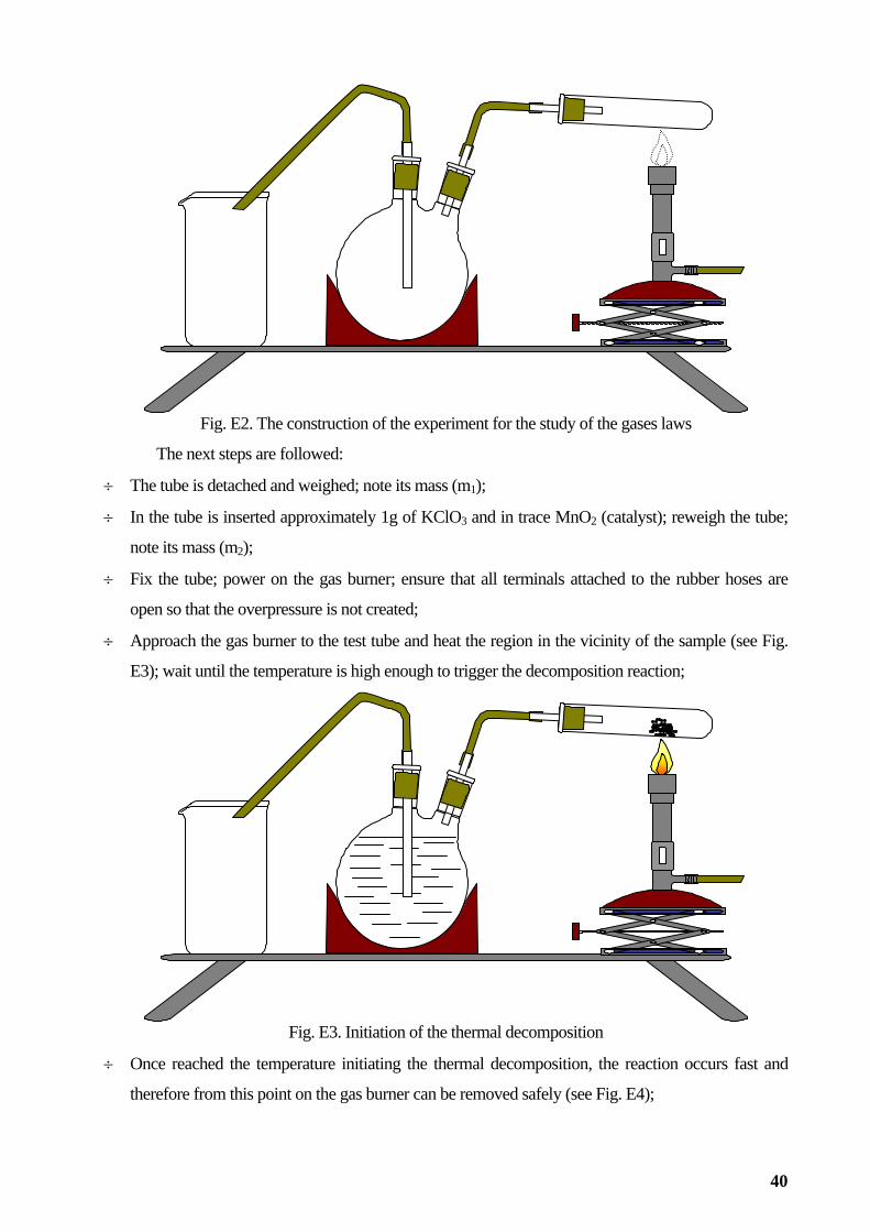
Fig. E2. The construction of the experiment for the study of the gases laws

The next steps are followed:

÷ The tube is detached and weighed; note its mass (m1);

÷ In the tube is inserted approximately 1g of KClO3 and in trace MnO2 (catalyst); reweigh the tube;

note its mass (m2);

÷ Fix the tube; power on the gas burner; ensure that all terminals attached to the rubber hoses are

open so that the overpressure is not created;

÷ Approach the gas burner to the test tube and heat the region in the vicinity of the sample (see Fig.

E3); wait until the temperature position reaction;

itiation of the thermal decomposition

Onc

ner can be removed safely (see Fig. E4);

is high enough to trigger the decom

Fig. E3. In

÷ e reached the temperature initiating the thermal decomposition, the reaction occurs fast and

therefore from this point on the gas bur

40

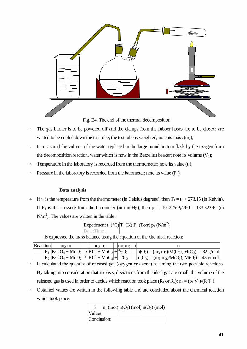
The gas burner is to be powered off and the clamps from the rubber hoses are to be closed; are

eighted; note its mass (m3);

eaction, water which is now in the Berzelius beaker; note its volume (V1);

e barometer; note its value (P1);

÷ If t1 is the temperature from the thermometer (in Celsius degrees), then T1 = t1 + 273.15 (in Kelvin).

If P1 is the pressure from the barometer (in mmHg), then p1 = 101325·P1/760 = 133.322·P1 (in

N/m2). The values are written in the table:

Experiment t1 (°C) T1 (K) P1 (Torr) p1 (N/m2)

Fig. E4. The end of the thermal decomposition

÷

waited to be cooled down the test tube; the test tube is w

÷ Is measured the volume of the water replaced in the large round bottom flask by the oxygen from

the decomposition r

÷ Temperature in the laboratory is recorded from the thermometer; note its value (t1);

÷ Pressure in the laboratory is recorded from th

Data analysis

Date:Time Is expressed the mass balance using the equation of the chemical reaction:

Reaction m2-m1 m3-m1 m3-m2 → n R1: KClO4 + MnO2 → KCl + MnO2 + 3/2O2 n(O2) = (m3-m2)/M(O2); M(O2) = 32 g/molR2: KClO4 + MnO2 ? KCl + MnO2 + 2O3 n(O3) = (m3-m2)/M(O3); M(O3) = 48 g/mol

÷ Is calculated the quantity of released gas (oxygen or ozone) assuming the two possible reactions.

By taking into consideration that it exists, deviations from the ideal gas are small, the volume of the

released gas is used in order to decide which reaction took place (R1 or R2): n1 = (p1·V1)/(R·T1)

÷ Obtained values are wr out the chemical reaction itten in the following table and are concluded ab

which took place:

? n1 (mol) n(O2) (mol) n(O3) (mol)Values Conclusion:

41

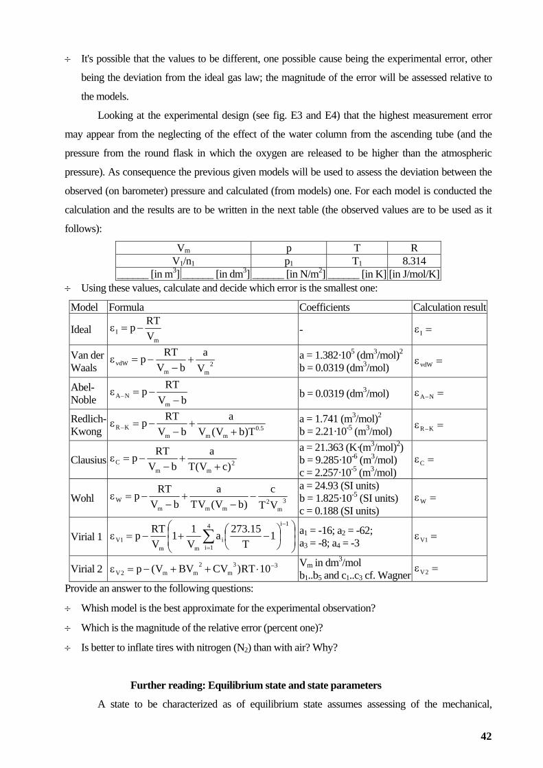
÷ It's possible that the values to be different, one possible cause being the experimental error, other

being the deviation from the ideal gas law; the magnitude of the error will be assessed relative to

the models.

Looking at the experimental design (see fig. E3 and E4) that the highest measurement error

may appear from the neglecting of the effect of the water column from the ascending tube (and the

pressure from the round flask in which the oxygen are released to be higher than the atmospheric

pressure). As consequence the previous given models will be used to assess the deviation between the

observed (on barometer) pressure and calculated (from models) one. For each model is conducted the

calculation and the results are to be written in the next table (the observed values are to be used as it

follows):

Vm p T R V 8.314 1/n1 p1 T1

______ [in m3] ______ [in dm ] ______ [in N/m ] ______ [in K] [in J/mol/K] 3 2

÷ Using these values, calculate and decide which error is the smallest one:

Model Formula Coefficients Calculation result

Ideal m

I VRTp −=ε - =εI

Van der Waals 2vdW V

abV

RTp +−

−=ε a = 1.382·105 (dm3/mol)2 b = 0.0319 (dm3/mol)

εvdWmm

=

Abel- Noble bV

pm

NA −−=ε − b = 0.0319 (dm /mol)

RT 3 =ε −NA

Redlich- Kwong 5.0KR

aε − a = 1.741 (m3/mol)2

-5 3mmm T)bV(VbV +− b = 2.21·10 (m /mol)

RTp +−= =ε −KR

Clausius 2mm

C )cV(Ta

bVRTp

++

−−=ε

a = 21.363 (K·(m3/mol)2) b = 9.285·10-6 (m3/mol) =εC c = 2.257·10-5 (m3/mol)

Wohl 3c

mmW VTbV

RTp−

−=εa = 24.93 (SI units)

units) c = 0.188 (SI units)

2mm V(VT )

−b

a−

+ b = 1.825·10-5 (SI =εW

Virial 1 ⎟⎟

a⎠

⎞⎛ ⎞⎛−4 1i15.2731RT a = -16; a = -62;

⎜⎜= ∑1V 1 1 2

= -8; a = -3 ⎝m⎟⎠

−1⎜⎝

ia+−V

pε=1im TV 3 4

=ε 1V

Virial 1 V2 ε 30− 32 RT)CV+ mmm2V b1..b5 and c1..c3 cf. Wagner BV(p +−= V ⋅ m in dm /mol =ε 2V 3

Provide an answer to the following questions:

÷ Whish model is the best approximate for the experimental observation?

÷ Which is the magnitude of the relative error (percent one)?

2÷ Is better to inflate tires with nitrogen (N ) than with air? Why?

Further readin

A state to be characterized as of equilibrium state assumes assessing of the mechanical,

g: Equilibrium state and state parameters

42

thermal, and chemical equilibrium. At least the definition of the chemical equilibrium assumes the

existence of a stationary state (in time) and from this point of view an immediate consequence is the

reflexivity of the equilibrium: if A is in equilibrium, then A is in equilibrium with A. Also the

symmetry of the equilibrium must be accepted: if A is in equilibrium with B, then B is in equilibrium

with A. More, the transitivity is assured too ("zero's principle of the thermodynamics"): if A in

equilibrium with B, and B in equilibrium with C, then A is in equilibrium with C, thus the equilibrium

concept defines an equivalence relation between systems (see next figure; the concept of equilibrium is

at the basis of the construction of many instruments, including the thermometer). Reflexive A (EQ) A Symmetric If [A (EQ) B] then [B (EQ) A] Transitive If [A (EQ) B] & [B (EQ) C] then [A (EQ) C]

Equivalence (EQ) Reflexive & ymmetric & Tra ve S nsiti

A state is defined lly using a series of i bservable pr ties. To mbered is that

d being not

generally known. Defining of a property as a state param

observe it on the systems being in equilibrium. State parameters can be categorized as is shown in the

n

+ State parameters

genera ts o oper be reme

the necessary number of parameters to define a state of a system depends on the system an

eter is directly linked by our capacity to

ext:

- Structure - Energy - Quantity - ? ... Density (ρ) Temperature (T) Mass (m) ... Pressure (p) Internal energy (E) Volume (V) Molar mass (M ) Enthalpy (H) Particle's number (N) Entropy (S) Gibbs's free energy (G) ... Chemical composition (F) Helmholtz' enes free rgy (H) Fugacity (f) Exergy (B) ... ...

racteristic to the state parame rs (or functions) is that it not depends on the succession of

processes through the system evolved to arrive at. In other words, any closed path followed by a

process will bring the system in the same state, c a

parameters. By contrast, all parameters depending on the succession of th

s olved enter in the category of parameters of p (mechanical, electrical) and

heat are parameters of process.

Cha te

h racterized by the same values for the state

e processes through which

ystem ev rocess. Thus, work

43

Qualitative analysis of metals and alloys

Introduction

There are many methods for analyzing samples containing metals, some of them conducting

the analysis with the sample in solid state or after passing the metals into a solution as cations.

With regard to the 'qualitative' word meaning, a qualitative method is intended to be used to

provide a 'Yes/No' answer to the question if a (certain) metal is present in the sample, while a

quantitative method is intended to be used to provide a quantity (with measurement units such as mass

or volume) or a ratio (or a ge) of tal in the sample. It exists also

methods called 'semi-quantitative' of equisite for the other two

categories.

icro-quantities. The modern apparatus for analysis generally couple chemical with instrumental

methods to provide both qualitative and quantitative information about the composition of the samples.

Other pa he set of th

part of or whole irrevers s during th estructive (when no

changes or revers le).

Some of s provide a tion correlated with the quantity (of the metal in the

mple

device is sometimes called electrograph, but due to simplicity of its use

is better called metal ionizer.

Purpose

The purpose of the laboratory activity is to qualitatively analyze a series of metallic samples.

Therefore, each student will analyze one sample.

Material and method

The principle of analysis works the same at this device as it works for a modern device which is

percenta representation of the me

which intend is to be used as prer

Other classification of the methods takes into consideration the size of the (required) sample,

and from this point of view, the methods may be intended for macro (quantities) when the size is about

100mg, semi-micro (size about 10 mg), micro (~ 1 mg), ultra-micro (~ 1 μg) and sub-micro (~ 10 ng).

Chemical methods are generally involved for macro-quantities, while instrumental methods are

for m

rtition on t e analysis methods divide the methods in destructive (when a

sample suffers ible change e analysis) and nond

ible changes are applied to a part or whole samp

the method n informa

sa ), and then are called absolute or stoechiometric methods while others provide an information

correlated with the ratio (or proportion of the metal in the sample), and then are called relative or non-

stoechiometric methods, tracing the metals being an important issue in environmental science [171].

The experiment which will be conducted in the laboratory it uses an apparatus to disrupt from

the surface of the sample the metals and to pass it into a solution as cations with the help of the

continuous electric current. The

44

able to identify the metals l ionizer is coupled in an

electric circuit with an adjustable voltage source (usually with a feature producing a known potential-

intensity-time recording device.

ng NO3-

based on their oxidation potential, and then the meta

time curve) as well as with a potential-

The metallic sample is placed between the plates of the metal ionizer, and between the sample

and the positive charged plate is placed a filter paper moistened with a solution of containi

anions. Connecting the device to the power source operating with a potential in 2-6V range will pass

atoms of the metals from the sample to the filter paper as cations combining it with the NO3- anions:

Me0 - ne- → Men+ Sample (containing Me0) is connected at anode (+), passing thus the electrons (ne-) through the electric circuit

Filter paper (containing Men+) is connected at cathode (-), allowing the metallic cations to migrate to it and discharge on it

It’s a general rule that salts containing nitrate ion (NO3

-) are soluble. Other discharges are

possible too at the cathode, for the other ions present in the solution. Thus, writing the dissociation of

the water, it is clear that also hydrogen ions (named 'hydron') may discharge. Which ion actually

discharge it depend on the oxidation potential of the metal (and for the competition with hydron, if this

potential is positive or not; a negative electrode potential indicate that hydrogen discharge in the place

of the metallic cation).

H2O ↔ H+ + HO- 2H+ + 2e- → H2 Men+ + ne- → Me0 water dissociation possible reactions at cathode

As can be seen from the previous table, consuming of the hydrons from the water may lead to a

basic solution (with a pH greater than 7), when the cations of the metal may combine with hydroxide

O-) t

c ons

ence of air and moisture, covering itself with an

olating layer of oxide and/or hydroxide), a filter paper, a nitrate solution (usually 5% NaNO3), a nitric

O3), of the metal ionizer along with the power source (see the next

(H o form hydroxides (Me(OH)n). This is an unwanted outcome, because most of the hydroxides

are only slightly soluble, and we need to have soluble combinations of the cations from at least two

reasons: to keep the conduction of the current trough the circuit long enough to pass as many as

possible metallic cations on the filter paper as well as for the next stage, analysis of the metallic ati

with a series of specific reactions is necessary to have soluble compounds of it in order to make

possible the aqueous reaction with the reagents.

To conduct one experiment of sample analysis, is necessary the sample, some abrasive paper to

polish the sample (some metals oxidizes in the pres

is

acid solution (usually diluted HN

figure) as well as a series of reagents to conduct the specific reactions for cations identification.

45

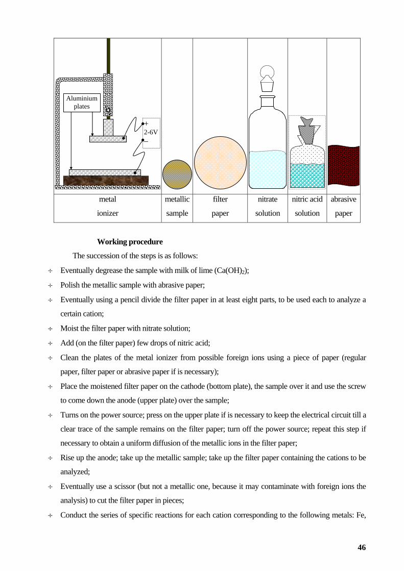
46

+ 2-6V

–

Aluminium plates

metal

ionizer

metallic

sample

filter

paper

nitrate

solution

nitric acid

solution

abrasive

paper

Working procedure

The succession of the steps is as follows:

÷ Eventually degreas

÷ Polish the metallic e pa

Eve

e sample;

Tur

÷ Eventually use a scissor (but not a metallic one, because it may contaminate with foreign ions the

analysis) to cut the filter paper in pieces;

÷ Conduct the series of specific reactions for each cation corresponding to the following metals: Fe,

e the sample with milk of lime (Ca(OH)2);

sample with abrasiv per;

÷ ntually using a pencil divide the filter paper in at least eight parts, to be used each to analyze a

certain cation;

÷ Moist the filter paper with nitrate solution;

÷ Add (on the filter paper) few drops of nitric acid;

÷ Clean the plates of the metal ionizer from possible foreign ions using a piece of paper (regular

paper, filter paper or abrasive paper if is necessary);

÷ Place the moistened filter paper on the cathode (bottom plate), the sample over it and use the screw

to come down the anode (upper plate) over th

÷ ns on the power source; press on the upper plate if is necessary to keep the electrical circuit till a

clear trace of the sample remains on the filter paper; turn off the power source; repeat this step if

necessary to obtain a uniform diffusion of the metallic ions in the filter paper;

÷ Rise up the anode; take up the metallic sample; take up the filter paper containing the cations to be

analyzed;

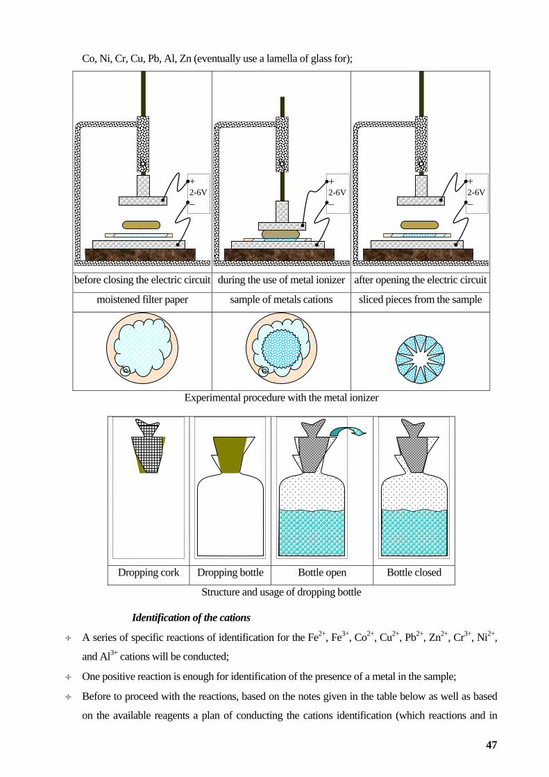
Co, Ni, Cr, Cu, Pb, Al, Zn (eventually use a lamella of glass for);

+ 2-6V

–

+ 2-6V

–

+ 2-6V

–

before closing the electric circuit during th e of m nizer e us etal io after opening the electric circuit

moistened filter paper esample of m tals cations sliced pieces from the sample

Experimental procedure with the metal ionizer

Dropping cork Dropping bottle Bottle open Bottle closed

Structure and usage of dropping bottle Identification of the cations

÷ A series of specific reactions of identification for the Fe2+, Fe3+, Co2+, Cu2+, Pb2+, Zn2+, Cr3+, Ni2+, 3+

fication of the presence of a metal in the sample;

on the available reagents a plan of conducting the cations identification (which reactions and in

and Al cations will be conducted;

÷ One positive reaction is enough for identi

÷ Before to proceed with the reactions, based on the notes given in the table below as well as based

47

which succession) should be written;

÷ The series of the reactions is in the following table:

Cation + Reagents → Products Color NoteFe2+ + K3Fe(CN)6 → Fe3[Fe(CN)6]2 + K+ blue 1 + NaOH → Fe(OH)2 + Na+ gray-green air→ red-brown + DMG → Fe(DMG)2 + H+ red + Dipyridile → Fe(dipyridile)2

2+ purple red Fe3+ + K4Fe(CN)6 → Fe4[Fe(CN)6]3 + K+ blue 2 + NH4OH → Fe(OH)3 + NH4

+ reddish brown 3 + NH4SCN → Fe(SCN)3 + NH4

+ red 4 + CH3COONa → Fe(CH3COO)3 + Na+ red-brown + CH3COONa + KI → Fe(CH3COO)2 + I2 + Na+ + K+ brown + Sulphosalicylic acid → Fe(sulphosalicylate) + H+ at pH∈[1.8,2.5], red-violet Co2+ + NH4SCN → Co(NH4)2(SCN)4 + NH4

+ blue 4 + NH4OH + DMG → Co(DMG)2 + H+ + H2O dark brown 5 + NO3

- + Al2(SO4)3 → Co(AlO2)2 + NO2 + O2 + SO3 Tenard's blue at ignition 6 + NO3

- + Zn(NO3)2 → CoZnO2 + NO2 + O2 Rinmann’s green at ignition 7 + NH4OH + H2O2 → Co(NH3)5

3+ + H2O red + NaOH → Co(OH)- heating→ Co(OH)2 air→ Co(OH)2

1+ dark blue heating→ rose air→ brown Cu2+ + NH OH → Cu(N4 H ) (OH) + H+ + H O in3 4 t2 2 ense blue 3 4[Fe(CN red-+ K4Fe(CN)6 → Fe )6] + K+ brown 2 + Cuprone → Cu(cuprone) + H dark green flame→ dark blue or green +

Pb2+ + KI → PbI2 + K+ yellow + K2CrO4 → PbCrO4 + K+ yellow Sn4+ + Cupferron + NH4OH → Sn(cupferron)4 + H+ + H2O yellow Zn2+ + K3Fe(CN)6 → Zn3[Fe(CN)6]2 + K+ white to green when heated 1 + NO3

- + Co(NO3)2 → CoZnO2 + NO2 + O2 Rinmann’s green at ignition 7 + Dithizone → Zn(dithizone)2 + H+ red 8 Cr3+ + NH4OH → Cr(OH) + NH + gray-green 3 3 4 + H2O2 (+ NaOH) → (CrO4)2- + H2O (+ Na+) yellow + H2O2 (+ HCl) → H2Cr2O7 + H + H2 (+ Cl nge + -) oraNi2+ + NH4OH → Ni(NH3)6(OH)2 + H+ + H2O blue 3 + NH4OH + DMG → Ni(DMG)2 + H+ + H2O red 5 + Na2HPO4 → Ni3(PO4)2 green Al3+ + NH4OH → Al(OH)3 + NH4

+ white gelatinous 3 + Alizarin + NH4OH → Al(alizarin)3 + H2O + NH4

+ red + Oxyne → Al(oxyne)3 + H+ yellow Mg2+ + Oxyne + NaOH → Mg(oxyne)2 fluorescing green

÷ Please read carefully the notes before proceeding with the identification of the cations: Note Comment 1 Fe2+ and Zn2+ both reacts selective with K3Fe(CN)6 2 Other cations that react with K4Fe(CN)6 to form highly colored precipitates must be absent (Co2+ and Fe3+ for example) 3 As is expected, when more t from Fe3+, Cu2+, Cr3+, Ni2+, Al3+ is present in sample, the reacti h

NH4OH is not conclusive fo he presence of any one han one cation r t

on wit

4 in the pre nd of the ssible wit presence of (by extracting it in) a mix of amyl

sence of both Fe3+ a Co2+ the identification Co2+ (blue) is po h NH4SCN in the alcohol and ether

5 Co2+ and Ni2+ both reacts selective with DMG(II) 6 When filter paper containing Co(NO ) and Al (SO4)3 is ignited produces an blue ash; reaction works in both senses, to

ide fy Co ( the filter paper and after migration of the Co(NO3)2 the Al2(SO4)3 is added), and to identify Al (when Na SO and H SO is add

3 2 2nti when NaNO3 and HNO3 is added on

2 4 2 4 ed on the filter paper and after migration of the Al2(SO4)3 theCo(NO3)2 is added)

7 reaction works in both senses, to identify C 2+ 2+

added) o (when Zn(NO3)2 is added), and to identify Zn (when Co(NO3)2 is

8 forms a red complex soluble in organic solvents (such as benzene, toluene, etc) ÷ The substances from the reactions table have the chemical structural formulas and reacts as is given

in the next table:

48

Name Chemical formula Complex DMG

HO N C CH

C CH3NHO

3 CH3C

CH3C N

O

N C CH3

C CH3N

OH

NNi

OH O Dipyridile

N

N

NN

NNFe

2-

sulphosalicylic O OHacid C

HO

SO OH

O

C

HO

O O

SO

O

O

Fe OH

Cuprone

C OHH5C6

C N OH

H

C6H5

C

C

H

C

H5C6

N O

O Cu

6H5 Cupferron

H

HN

O H

O

N

H

C H

O

H5C6 N C6H5NO

O

C H5

O

Sn

6 5

NO

O

O

6

NO

Dithizone

C SH

N

N

N

N

H

C6H5C6H5

C

N

SC

N

S

C6H5

Zn

5

NN

NHN

NHN

C6H

Alizarin O OH

O

OH O

O

O

O

AlOH

Oxyne

N

OH

NO

N OMg

÷ Depending on the result of the identification (Yes/No) following table will be filled.

49

Sample Ca o2+ Cu 2+ Cr3+ Ni2+ Al3+ tions→ Fe2+ Fe3+ C 2+ Pb2+ ZnName→

Flame test

÷ When the previous reactions are not conclusive, can be proceeded further to see the color in the

flame (by burning the filter paper with the sample of the metal ion on it);

÷ Following table contains the known color for the flame (thermal excitation) of the metallic cations:

Ion Flame color Cr2+ silver white Cr3+ violet (in the presence of NO3

-) Cr6+ orange Ni2+ bluish-green Mn2+ pink Pb2+ light blue Zn2+ light green Cu2+ bluish-green Cu(NH3)4

2+ dark blue FeSCN2+ red-brown (wine-red to dark-orange) Al3+ silver-white; in very hot flame light-blue Na+ yellow-orange K+ purple

Interpretation of the results

÷ The (previous) table will contain all the results obtained in a group of students;

÷ Each student labels its samp with its name;

÷ For its sample each student will write (again) the identification reactions (only) for the identified

cations;

÷ For each written (again) reaction the coefficients (conserving the number of atoms for each species

from reactants to products) must be established;

÷ To do at home: based on the (metals) content of the sample please use the literature (available on

Internet for instance) to identify the name of the alloy (if available and if applies) from which the

sample was taken (see also [172] and [173]).

Further reading

Actually the analysis of the cations requires (as is supposed to be observed from conducting the

experiments) separation of them in smaller groups in order to avoid the interference of one to another in

the identification process (see also [174]). This separation can be conducted on 'analytical groups' when

based on their selectivity (to react and on the properties of the compounds) with a series of anions, the

cations are divided in groups, as the following image shows:

le

50

pH=0.5; H2S (exs)

Pp: Hg2Cl2, AgCl, PbCl2

KOH

Pp: Bi2S3, HgS, PbS, CuS, CdS

Sol: SbS2-, Sb(OH)4-,

HgS2-, AsO2

-, AsS2-,

Sn(OH)62-, SnS3

2-

HCl(dil) N NH3 + H4Cl H2S

Pp: CoS, MnS, ZnS, NiS, Fe2S3, Al(OH)3, Cr(OH)3

H2O; NH4Cl; (NH4)2CO3 CH3COOH

Sol: Mg2+, Na+, K+

Pp: BaCO3, SrCO3, CaCO3, MgCO3 Of course that th aration and the general idea is to combine in the analysis

chemical with instrumen thods ( 178]).

e sep can continue

tal me see also [131], [175], [176], [177] and [

51

Study of chemical reactions

Introduction

In general, a chemical reaction may be defined as a process that leads to the transformation of

one set of chemical substances (called reactants or reagents) to another (called products), in which the

changes involve only the positions of electrons in the forming and breaking of chemical bonds between

atoms (with no change to the nuclei).

participants the chemical reactions are described with chemical equations, which graphically present

the starting materials, end products, and sometimes intermediate products and reaction conditions. A

chemical equation is written in general as "Reactants → Products", in which the "→" symbol express

the creation of the reaction products ("Products") from the reactants ("Reactants"). A concept related to

the chemical reaction concept is chemical equilibrium. Theoretically all chemical reactions evolves to

an equilibrium between the reactants and the products but in some cases this equilibrium may be

shifted to the left (to the reactants) or to the right (to the products), and it depends on a series of factors

including temperature, pressure, environment (for instance catalysts) and the interaction of the system

of reaction with it (the system of reaction may be 'open' meaning that is possible the transfer of the

substance to and from environment, or may be 'closed', meaning that no transfer with the environment

is allowed).

In a system is possible to move the chemical equilibrium if the transformation is accompanied

by a transfer of substance (to and from environment). Thus, the Zn(s) + 2HCl(aq) → ZnCl2(aq) + H2(g)

reaction, with occurs at the contact surface between Zn (solid) and HCl solution (liquid) is a 'total'

reaction if the released hydrogen leaves the system (for instance if the surface of the liquid is in contact

with the atmosphere, where H2 arrives, being thus send away from reaction environment). In these

cases it may be considered that the reactions are total (the entire quantity of Zn or the entire quantity of

HCl are consumed - whichever is the first).

A chemical reaction is named 'total' if the equilibrium is strongly shifted to the right, meaning

that at the end of the reaction very little quantity (negligible) of reactants is still present in the system

(of reaction). The applications of the total reactions include the chemical methods for determining the

chemical composition, and are applied on large scale for reactions in aqueous environment. Total

reactions may be found between:

÷ Acid-base reactions. An acid-base reaction involves a transfer of protons (H+, H3O+) from one

species (the acid) to another (the base). A special case of the acid-base reaction is the neutralization

where an acid and a base, form a salt and water.

A chemical process may involve more than a chemical reaction and then a chemical reaction is

the transformation in which the participants (the reactants and the products) are known. For defined

52

÷ Precipitation. Precipitation is t (or inside another solid) during a

chemical reaction. It usually takes place when the concentration of dissolved ions exceeds the

ble salt. For some applications, see [179], [180].

Com

pairs of the ligand into empty orbitals of the central atom(s) and

form

reactants and (βj)1≤j≤n are the coefficients of the (Pj)1≤j≤n products, the principle of number

d).

the products are: a1·α1/α1, a1·α2/α1, …, a1·αm/α1 (in same units as a1).

4], [185], [186] as examples);

he formation of a solid in a solution

solubility limit and forms an insolu

÷ plexation. In complexation reactions, several ligands (they can be both ions and neutral

molecules, such as carbon monoxide, ammonia or water) react with one (or more) 'central' atom

(usually a metallic one) to form a coordination complex (ligands surrounding the central atoms).

This is achieved by providing lone

ing dipolar bonds. Complexation reactions also include ligand exchange, in which one or more

ligands are replaced by another, and redox processes (see also [181]) which change the oxidation

state of the central atom(s).

An important task dealing with chemical total reactions is the establishing of the ratios between

the participants. These ratios result by natural way, applying the conservation principles operating

during reactions, which are translated in the chemical reaction equation as coefficients of the

participants. For classical chemical reactions (not including here transformations at the level of the

atoms nucleuses) when the electrical current is not involved is applied the principle of number of

atoms (for each element) conservation which postulates that for each element (let be 'E' an element)

the number of atoms (let be N('E',U) the number of E atoms in the U chemical compound) before

(reaction) is equal with the number of atoms after (reaction).

For an reaction expressed as: Σ1≤i≤mαiRi → Σ1≤j≤nβjPj, in which (αi)1≤i≤m are the coefficients of

the (Ri)1≤i≤m

of atoms conservation provides one equality relationship for each element: Σ1≤i≤mαi·N('E',Ri) =

Σ1≤j≤nβj·N('E',Pj).

Turning back to aqueous environments, when conducting reactions in, an important point for

the 'total' reactions is the equivalence point, defined as the moment, when (at least a part of the)

reactants react wholly, when, based on the equation of the chemical reaction is possible to obtain the

quantity of the reactants consumed when one of them is known (for instance by adding it in small

quantities till the equivalence point is reache

Considering thus the general reaction α1R1 + Σ2≤i≤mαiRi → Σ1≤j≤nβjPj when a known quantity (in

number of molecules, or, more convenient, in number of moles) of the R1 reactant, let's say a1 (moles)

is added in the reaction system till the moment when the equivalence point of the reaction is reached,

then at least one of the other reactants (from R2 to Rm) is completely consumed, and the quantities of

the reactants which reacted to form

Of practical importance when conducting chemical reactions in aqueous solutions is expressing

of the concentration on different scales, given in the next table (L = dm3), because most of the chemical

reactions occurs in aqueous phase (see [182], [183], [18

53

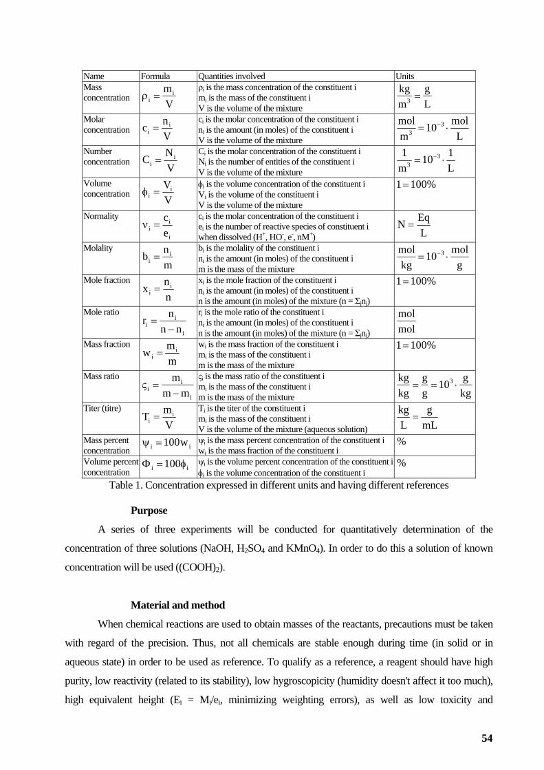
Name Formula Quantities involved Units Mass concentration V

mii =ρ

ρi is the mass concentration of the constituent i mi is the mass of the constituent i V is the volume of the mixture m

kg3 = L

g

Molar concentration V

nc ii =

ci is the molar concentration of the constituent i ni is the amount (in moles) of the constituent i V is the volume of the mixture L

mol10mmol 3

3 ⋅= −

Number concentration V

NC ii =

Ci is the molar concentration of the constituent i Ni is the number of entities of the constituent i V is the volume of the mixture L

110m1 3

3 ⋅= −

Volume concentration V

Vii =φ

φi is the volume concentration of the constituent i Vi is the volume of the constituent i V is the volume of the mixture

%1001=

Normality

i

ii e

c=ν

ci is the molar concentration of the constituent i ei is the number of reactive species of constituent i when dissolved (H+, HO-, e-, nM+) L

N = Eq

Molality

mnb i

i = bi is the molality of the constituent i ni is the amount (in moles) of the constituent i m is the mass of the mixture g

mol10kg

mol 3 ⋅= −

Mole fraction

nnx i

i = xi is the mole fraction of the constituent i ni is the amount (in moles) of the constituent i n is the amount (in moles) of the mixture (n = Σjnj)

%1001=

Mole ratio

i

ii nn

nr−

= ri is the mole ratio of the constituent i ni is the amount (in moles) of the constituent i n is the amount (in moles) of the mixture (n = Σjnj) mol

mol

Mass fraction

mmw i

i = wi is the mass fraction of the constituent i mi is the mass of the constituent i m is the mass of the mixture

%1001=

Mass ratio

imm − m is the mass of the mixture

ii

m=ς

ςi is the mass ratio of the constituentmi is the mass of the constituent i

i

kggkgg10gkg 3 ⋅==

Titer (titre)

VmT i

i = T is the titer of the constituent i mi is the mass of the constituent i V is the volume of the mixture (aqueous solution)

i

mLg

Lkg

=

Mass percent oncentration ii w100=ψ ψi is the mass percent concentration of the constituent i %

c wi is the mass fraction of the constituent i Volume percent con

100centration ii φ=Φ ψi is the volume percent concentration of the constituent i %

φi is the volume concentration of the constituent i Table 1. Concentration expressed in different units and having different references

Purpose

A series of three experiments will be conducted for quantitatively determination of the

concentration of three solutions (NaOH, H2SO4 and KMnO4). In order to do this a solution of known

as low toxicity and

concentration will be used ((COOH)2).

Material and method

When chemical reactions are used to obtain masses of the reactants, precautions must be taken

with regard of the precision. Thus, not all chemicals are stable enough during time (in solid or in

aqueous state) in order to be used as reference. To qualify as a reference, a reagent should have high

purity, low reactivity (related to its stability), low hygroscopicity (humidity doesn't affect it too much),

high equivalent height (Ei = Mi/ei, minimizing weighting errors), as well

54

availability.

en is wa n solid state crystallizes with two water molecules,

(CO can be u d a using a solution of an known

conc on of oxalic acid can of other reactants which reacts

with l applicati n of g it in a reaction with a base, as

follo

1(COOH)2 + 2 2O where M can be K or Na

hydroxi e (K oiting its reactivity

tow nd its corrosive n or to most soft and liquid soaps

as well as numerous pot sium xide is usuall available as

translucent pellets, which will b H is hygroscopic. Consequently, KOH

typically contains varying amo r the preparation of the KOH

solu n conce rati

solved by determining its conte on reactions (as the reaction

with oxalic acid). About the NaOH), being a caustic reagent

that d to neutralize agents. It is also used in a variety of

large scale applications, such as g, the manufacture of soap and detergents,

and water treatment. These alka escent and readily absorb moisture and

carbon dioxide in air.

Their solutions are it ormation of carbonat tion

(KO KHCO3; KH → NaHCO3; NaHCO3 +

NaO 3 + H2O). D uti n, when KOH (or

NaO is titred with an points, one corresponding to

e total co CO2

+ H2O → H2C formation of H2CO3. This is the reason for which the KOH and NaOH

lution

determinations.

Once determined the concentration of the base (MOH) this base can be further used to

ing:

Wh solved in ter, oxalic acid (i

OH)2·2H2O) se s analytical standard and therefore, by

entrati be obtained the corresponding quantity

it. A typica o the oxalic acid as reference is involvin

wing:

MOH → 1(COOM)2 + 2H

Potassium d OH) has many industrial and niche applications expl

ard acids a ature. KOH is noteworthy as the precurs

as -containing chemicals. Potassium hydro y

ecome tacky in air because KO

unts of water (as well as carbonates). Fo

tions of know nt ons, the water stored in its solid state is an inconvenient which can be

nt (in KOH) by involving it in neutralizati

same idea applies to sodium hydroxide (

is widely use acids and prepare sodium salts of re

pulp and paper manufacturin

lis (KOH and NaOH) are deliqu

w h a reduced stability in air, due to f e in solu

H + CO2 → CO3 + KOH → K2CO3 + H2O; NaOH + CO2

H → Na2CO ue to the presence of the carbonate ions in sol o

H) solution acid, its titration curve have two inflexion

ntent of K+ (or Na+) ions and other one corresponding to the moving of the equilibriumth

O3 to the

so s are not considered analytical standards, and should be prepared with precautions (by

expelling the carbon dioxide by boiling the solution or by purging it with an inert gas, [187]) determined

immediately before its use in quantitative

determine the concentration of an acid, as follow

2MOH + 1H2SO4 → 1M2SO4 + 2H2O or 1MOH + 1HNO3 → 1MNO3 + 1H2O

Potassium permanganate (KMnO4) may contain reduced products like manganese oxide MnO2

where the concentration of KMnO4 is changed after preparation because it dissociated via reducing

agents such as ammonia and organic substances in water; therefore, potassium permanganate must be

standardized before use it and keep it at least 7-10 days after preparation at dark place and in a dark

55

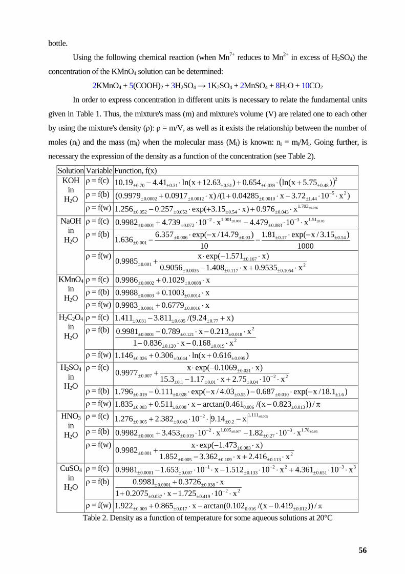
bottle.

Using the following chemical reaction (when Mn7+ reduces to Mn2+ in excess of H2SO4) the

concentration of the KMnO4 solution can be determined:

2KMnO4 + 5(COOH)2 + 3H2SO4 → 1K2SO4 + 2MnSO4 + 8H2O + 10CO2

In order to express concentration in different units is necessary to relate the fundamental units

given in Table 1. Thus, the mixture's mass (m) and mixture's volume (V) are related one to each other

by using the mix the number of

oles (

ture's density (ρ): ρ = m/V, as well as it exists the relationship between

m ni) and the mass (mi) when the molecular mass (Mi) is known: ni = mi/Mi. Going further, is

necessary the expression of the density as a function of the concentration (see Table 2).

Solution Variable Function, f(x) ρ = f(c) ( )248.0039.051.031.070.0 )75.5xln(654.0)63.12xln(41.419.10 ±±±±± +⋅++⋅− ρ = f(b) )x1072.3x04285.01/()x0917.09979.0( 25

44.10010.00012.00002.0 ⋅⋅−⋅+⋅+ −±±±±

KOH in

H2O ρ = f(w) 066.0703.1

043.054.0052.0052.0 x976.0)x15.3exp(257.0256.1 ±⋅+⋅+⋅− ±±±± ρ = f(c) 03.0008.0 51.13

083.0001.12

072.00001.0 x10479.4x10739.49982.0 ±± ⋅⋅−⋅⋅+ −±

−±±

ρ = f(b) 1000

)15.3/xexp(81.110

)79.14/xexp(357.6636.1 54.017.003.0006.0001.0

±±±±±

−⋅−

−⋅−

NaOH in

H2O

ρ = f(w) 2

1054.0117.00035.0

167.0001.0 x9535.0x408.19056.0

)x571.1exp(x9985.0⋅+⋅−

⋅−⋅+

±±±

±±

ρ = f(c) x1029.09986.0 0008.00002.0 ⋅+ ±± ρ = f(b) 0 x1003.09988. 0014.00003.0 ⋅+ ±±

KMnO4 in

H2O ρ = f(w) x6779.09983.0 0016.00001.0 ⋅+ ±± ρ = f(c) )x24.9/(811.3411.1 77.0605.0031.0 +− ±±± H Cρ = f(b)

2019.0120.0

2018.0121.00001.0

x168.0x836.01x213.0x789.09981.0

⋅−⋅−⋅−⋅−

±±

±±±

2 2O4 in

H2O

ρ = f(w) )616.0xln(306.0146.1 095.0044.0026.0 ±±± +⋅+ ρ = f(c)

2204.001.01.0

021.0007.0 x1075.2x17.13.15

)x1069.0exp(x9977.0⋅⋅+⋅−

⋅−⋅+ −

±±±

±±

ρ = f(b) )1.18/xexp(687.0)03.4/xexp(111.0796.1 6.1010.055.0028.0019.0 ±±±±± −⋅−−⋅−

H2SO4 in

H2O

ρ = f(w) π−−⋅+ ±±± /))823.0x/(461.0arctan(x511.0835.1 013.0006.0008.0003.0 ρ = f(c) 005.0111.12

043.0005.0 14.910382.2276.1 ±⋅⋅+ ±−

±± 2.0 x− ρ = f(b) 00.12− 03.0007.0

27.0019.00001.0 x1082.1x10453.39982.0 ⋅⋅−⋅⋅+ ±±± 78.135 ±± −

HNO3 in

H2O ρ = f(w)

2083.0

x416.2x2 ⋅+⋅ 113.0109.0005.0001.0 36.3852.1

)x473.1exp(x9982.0−

⋅−⋅+

±±

±±

±

ρ = f(c) 651.0

22133.0

1007.00001.0 1361.4x10512.1x10653.19981.0 ⋅+⋅⋅−⋅⋅− ±

−±

−±±

33 x0 ⋅−

ρ = f(b) 22

419.0037.0

038.00001.0

x10725.1x2075.01x3726.09981.0

⋅⋅−⋅+⋅+

−±±

±±

CuSO4 in

H

2O

ρ = f(w) π−−⋅+ ±±± /))419.0x/(102.0arctan(x865.0922.1 012.0016.0017.0009.0 Table 2. Density as a function of temperature for some aqueous solutions at 20°C

56

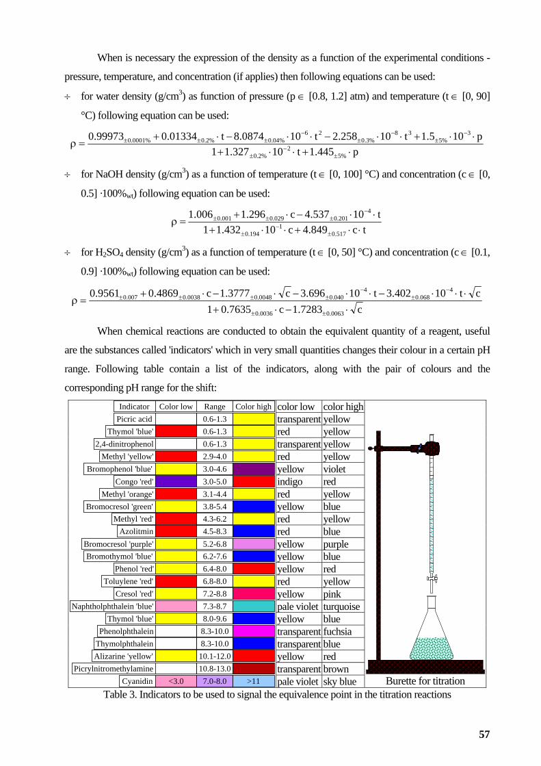
When is necessary the expression of the density as a function of the experimental conditions -

[0.8, 1.2] atm) and temperature (t ∈ [0, 90]

°C) follow

pressure, temperature, and concentration (if applies) then following equations can be used:

÷ for water density (g/cm3) as function of pressure (p ∈

ing equation can be used:

p445.1t10327.11p105.1t10258.2t100874.8t01334.099973.

%52

%2.0

3%5

38%3.0

26%04.0%2.0%0001.0

⋅+⋅⋅+⋅⋅+⋅⋅−⋅⋅−⋅+

=ρ±

−±

−±

−±

−±±±

÷ for NaOH density (g/cm3) as a function of temperature (t ∈ [0, 100] °C) and concentration (c ∈ [0,

0.5] ·100%wt) following equation can be used:

0

tc849.4c10432.11+=ρ

t10537.4c296.1006.1 4 ⋅⋅−⋅+ −

517.01

194.0

201.0029.0001.0

⋅⋅+⋅⋅ ±−

±

±±±

÷ fo 2S y (g/cm3) as a function of temperature (t ∈ [0, 50] °C) and concentration (c ∈

0 owing equation can be used:

r H O4 densit [0.1,

.9] ·100%wt) foll

c7283.1c7635.01ct10402.3t10696.3c3777.1c4869.

0063.00036.0

4068.0

4040.00048.00038.0

⋅−⋅+⋅⋅⋅−⋅⋅−⋅−⋅

ρ±±

−±

−±±±

When chemical reactions are conducted to obtain the equivalent quantity of a reagent, useful

are the substances called 'indicators' which in very small quantities changes their co ur in a certain pH

range. Following table contain a list of the indicators, along with the pair of colours and the

corres di

color low color high

01 007.0 +±956.0=

lo

pon ng pH range for the shift:

transparent yellow red yellow transparent yellow red yellow yellow violet indigo red red yellow yellow blue red yellow red blue yellow purple yellow blue yellow red red yellow yellow pink pale violet turquoiseyellow blue transparent fuchsia transparent blue yellow red transparent brown

Indicator Range Color low Picric acid

Color high 0.6-1.3

Thymol 'blue' 0.6-1.3 2,4-d l initropheno 0.6-1.3

Methyl 'yellow' 2.9-4.0 Bromop henol 'blue' 3.0-4.6

Congo 'red' 3.0-5.0 Methyl 'orange' 3.1-4.4

B ocresol 'rom green' 3.8-5.4 Methyl 'red' 4.3-6.2

Azolitmin 4.5-8.3 Bromocr esol 'purple' 5.2-6.8 Bromothymol 'blue' 6.2-7.6

Phenol 'red' 6.4-8.0 To ' luylene 'red 6.8-8.0

Cresol 'red' 7.2-8.8

Thymol 'blue' 8.0-9.6 Naphtholphthalein 'blue' 7.3-8.7

Phenolphthalein 8.3-10.0 Thym olphthalein 8.3-10.0 Alizarine 'yellow' 10.1-12.0

Picrylnitrom ethylamine 10.8-13.0Cyanidin >11 <3.0 7.0-8.0 pale violet sky blue

Burette for titration T able 3. Indicators to be used to signal the equivalence point in the titration reactions

57

Usually titrations are conducted adding distilled water in the flask such that at the beginning of

the titration to have the flask of about 1/3 full with reactive (see burette in Table 3).

Working procedure

For titration of NaOH with H2C2O4 the succession of the steps is as follows:

÷ Three samples of NaOH of known volumes (of about 5 ml, measured with the burette) are taken in

o The initial volume in the burette containing NaOH is recorded (Vinitial column in Table 4);

o The burette is used to take the approximate volume of NaOH given above;

is phenolphthalein) is added (to provide the change

of the colour of the solution when the equivalence point is passed); is added distilled water;

÷ By using the solution of oxalic acid (from the burette containing it) the titration of the sodium

hyd

nd H2C2O4 is conducted till the moment in which the indicator

indicate the equilibrium point (change in the co the solution);

o The final volume in the burette containing H Vfinal column in Table 4);

÷ The differences between initial and final volum as well as the average between

samples are calculated and recorded in Table 4.

1(COOH)2 + 2NaOH ON H2O

(three) Erlenmeyer flask(s), the results being recorded in Table 4. For each one out of three

samples:

o The final volume in the burette containing NaOH is recorded (Vfinal column in Table 4);

o One drop of indicator (usually the indicator

roxide is conducted for each of the three samples, the results being recorded in Table 4. For

each one out of three samples:

o The initial volume in the burette containing H2C2O4 is recorded (Vinitial column in Table 4);

o The reaction between NaOH a

lour of

2C2O4 is recorded (

es (ΔV), their ratio

→ 1(CO a)2 + 2 NaOH (ml) H2C2O4 (ml) Sample Vinitial Vfinal ΔV Vinitial Vfinal ΔV )Na(VΔ OH

OC22 )4H(VΔ⎟⎟⎠

⎞⎜⎜⎝

⎛ΔΔ

)NaOH(V)OCH(V 422 = Averagea1

1 2 3

a1 =

Table 4. Experimental data for titration of NaOH with H2C2O4

For titration of H2SO4 with NaOH the succe th s as follows:

÷ Three samples of H2SO4 of known volumes (of about 5 m sured with the burette) are taken in

(three) Erlenmeyer flask(s), the results being 5. For each one out of three

samples:

o The initial volume in the burette containing H (Vinitial column in Table 5);

o The burette is used to take the approximate v ven above;

o Th

o One drop of indicator (usually the indicator is phenolphthalein) is added (to provide the change

ssion of e steps i

l, mea

recorded in Table

2 4SO is recorded

olume of H2SO4 gi

e final volume in the burette containing H2SO4 is recorded (Vfinal column in Table 5);

58

of the colour of the solution when the equivalence point is passed); is added distilled water;

÷ By using the solution of sodium hydroxide (from the burette containing it) the titration of the

sulphuric acid is conducted for each of the three samples, the results being recorded in Table 5. For

o T ;

al volume in the burette containing NaOH is recorded (Vfinal column in Table 5);

tween

each one out of three samples:

he initial volume in the burette containing NaOH is recorded (Vinitial column in Table 5)

o The reaction between H2SO4 and NaOH is conducted till the moment in which the indicator

indicate the equilibrium point (change in the colour of the solution);

o The fin

÷ The differences between initial and final volumes (ΔV), their ratio as well as the average be

samples are calculated and recorded in Table 5.

2NaOH + 1H2SO4 → 1Na2SO4 + 2H2O H2SO4 (ml) NaOH (ml) Sample Vinitial Vfinal ΔV Vinitial Vfinal ΔV )SOH(V

)NaOH(V

42ΔΔ

⎟⎟⎠

⎞⎜⎜⎝

⎛ΔΔ

=)SOH(V)NaOH(VAveragea

422

1 2 3

a2 =

Table 5. Experimental data for titration of H2SO4 with NaOH

As preliminary for titration of (COOH)2 and H2SO4 with KMnO4 a calculation is conducted.

the

th (COOH)2 and is y =

2. The

H2SO4 solution

Known volumes (of about x = 5 ml, measured with the burette) of (COOH)2 will be taken (using

burette). Enough (to be corresponding) quantities of H2SO4 will be added (using the burette). The

corresponding quantity of H2SO4 is calculated from the equivalence wi

(3/5)·x/(a1·a2) ml, where a1 is from Table 4, a2 is from Table 5, x is the quantity of (COOH)

values are to be written in Table 6.

a1·a2 = (COOH)2 solutionVolume (in ml) x = y =

Tab 6. Equi ee d H2SO4 to be used for titration of KMnO4

In three Erle ws (repeated for each flask):

÷ Sample of x (ml) as approximate volume of (COOH)2 is take (recording initial volume, final

volume and their difference in Table 7);

÷ An approximate volum e, final volume

and their difference in Table 7);

this point on with the heated flask the titration with KMnO4 is conducted

n in Table 7);

4 (from

le valence betw n (COOH)2 an

nmeyer flasks, the succession of the steps is as follo

n into

e of y + 1 (ml) of H2SO4 is added (recording initial volum

÷ The flask is warmed up using a gas burner; the reaction requires heat in order to proceed fast; about

60° C are enough; from

manipulating the flask with a paper sleeve:

o The initial volume in the burette containing KMnO4 is recorded (Vinitial colum

o The reaction of between KMnO4 (from burette) with the mixture of H2SO4 and H2C2O

flask) is conducted till the moment in which the colour of the mixture in the flask become the

59

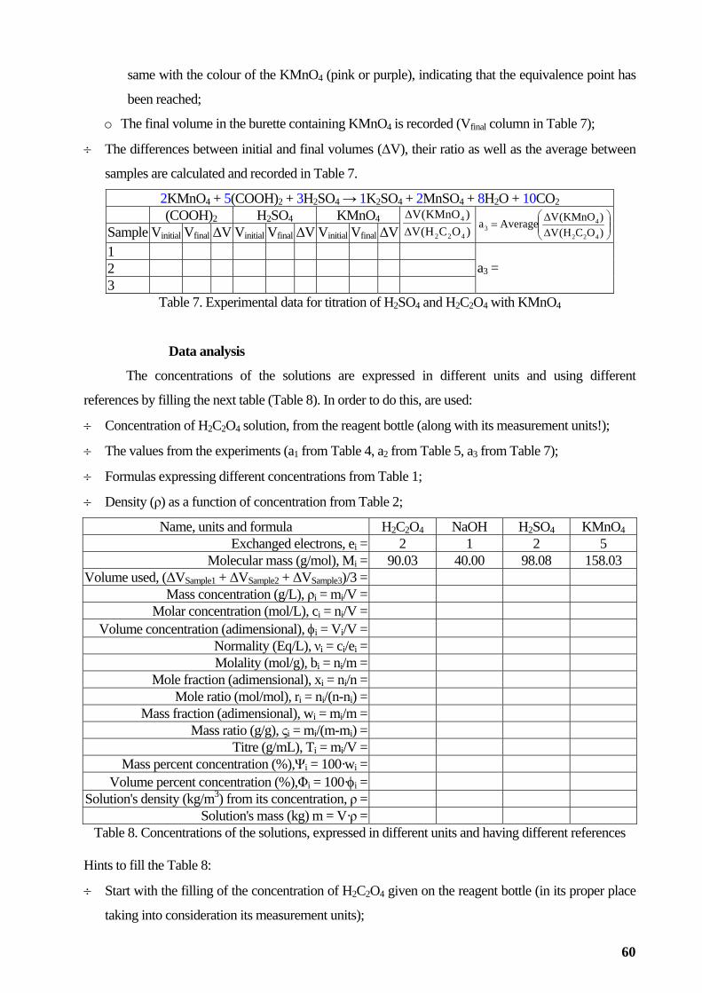
same with the colour of the KMnO4 (pink or purple), indicating that the equivalence point has

and final volumes (ΔV), their ratio as well as the average between

been reached;

o The final volume in the burette containing KMnO4 is recorded (Vfinal column in Table 7);

÷ The differences between initial

samples are calculated and recorded in Table 7.

2KMnO4 + 5(COOH)2 + 3H2SO4 → 1K2SO4 + 2MnSO4 + 8H2O + 10CO2 (COOH)2 H2SO4 KMnO4 Sample V V ΔV V V ΔV V V ΔVinitial final initial final initial final )OCH(V

)KMnO(V 4

ΔΔ

422⎟⎟⎠

⎞⎜⎜⎛ΔΔ

)OCH(V)KMnO(VAverage

4

4=a3⎝ 22

1 2 3

a3 =

Table 7. Experimental data for titration of H2SO4 and H2C2O4 with KMnO4

The concentrations of the solutions are expressed in different units and using different

references by ling t next tabl (T le 8). In order o do this, a d:

÷ Concentration of rement units!);

The

Data analysis

fil he e ab t re use

H2C2O4 solution, from the reagent bottle (along with its measu

÷ values from the experiments (a1 from Table 4, a2 from Table 5, a3 from Table 7);

÷ Formulas expressing different concentrations from Table 1;

÷ Density (ρ) as a function of concentration from Table 2;

Name, units and formula H2C2O4 NaOH H2SO4 KMnO4 Exchanged electrons, ei = 2 1 2 5

Molecular mass (g/mol), Mi = 90.03 40.00 98.08 158.03 Volume used, (ΔVSample1 + ΔVSample2 + ΔVSample3)/3 =

Mass conc (g/L), entration ρi = mi/V = Molar concen ni/V = tration (mol/L), ci =

Volume concentration (adimensional), φi = Vi/V = Normality (Eq/L), νi = ci/ei = Molality (mol/g), bi = ni/m =

Mole fraction (adimensional), xi = ni/n = Mole ratio (mol/mol), ri = ni/(n-ni) =

Mass fraction (adimensional), wi = mi/m = Mass ratio (g/g), ςi = mi/(m-mi) =

Titre (g/mL), Ti = mi/V = Mass percent concentration (%),Ψi = 100·wi =

Volume percent concentration (%),Φi = 100·φi = Solution's density (kg/m3) from its concentration, ρ =

Solution's mass (kg) m = V·ρ = Table 8. Concentrations of the solutions, expressed in different units and having different references

taking into consideration its measurement units);

Hints to fill the Table 8:

÷ Start with the filling of the concentration of H2C2O4 given on the reagent bottle (in its proper place

60

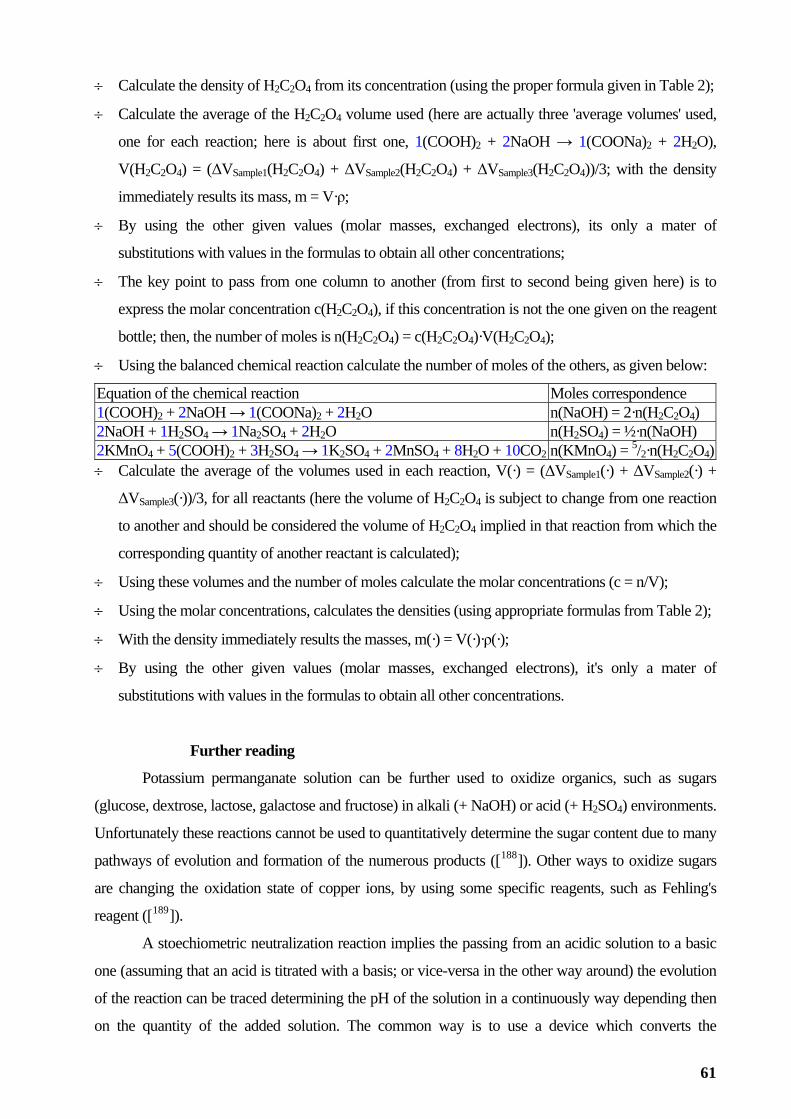
÷ Calculate the density of H2C2O4 from its concentration (using the proper formula given in Table 2);

÷ Calculate the average of the H2C2O4 volume used (here are actually three 'average volumes' used,

H2O),

÷ By using a mater of

er concentrations;

÷ e key oint o p s m one column to another (from first to second being given here) is to

ress the mo e tratio c(H C2 4), if his concentration is no ne given on the reagent

bottle; the

Using the balanced chemical reaction calculate the number of moles of the others, as given below:

on Moles correspondence

one for each reaction; here is about first one, 1(COOH)2 + 2NaOH → 1(COONa)2 + 2

V(H2C2O4) = (ΔVSample1(H2C2O4) + ΔVSample2(H2C2O4) + ΔVSample3(H2C2O4))/3; with the density

immediately results its mass, m = V·ρ;

the other given values (molar masses, exchanged electrons), its only

substitutions w vaith lues in eth rm fo ulas to ob n atai ll oth

Th p t as fro

exp lar conc n n 2 O t t the o

n, the number of moles is n(H2C2O4) = c(H2C2O4)·V(H2C2O4);

÷

Equation of the chemical reacti1( H)2 + 2NaOH → 1(COONa)2 + 2H2O n(NaOH) = 2·n(H2C2O4) COO2N + 1H2SO4 → 1Na2SO4 + 2H2O n(H2SO4) = ½·n(NaOH) aOH2KMnO4 + 5(COOH)2 + 3H2SO4 → 1K2SO4 + 2MnSO4 + 8H2O + 10CO2 n(KMnO4) = 5/2·n(H2C2O4)÷ Calculate the average of the volumes used in each reaction, V(·) = (ΔVSample1(·) + ΔVSample2(·) +

one reaction

plied in that reaction from which the

÷ Using these volum oles calcu olar concentrations (c = n/V)

÷ Using the molar concen sities (using appropriate formulas from Table 2);

y im (· ·ρ(·);

÷ By using s, exchanged electrons it's only a mater of

ll other con entrations.

Further

Pota ther used to oxidize organics, such as sugars

(glucose, d li (+ Na id ( H2SO4) environments.

Unfortunately these atively det mine the sugar content due to many

pathwa products 188]). Other ways to oxidize sugars

a sing some pecific rea ents, such s Fehling's

reagent ([ ]).

id is titrated with a basis; or vice-versa in the other way around) the evolution

ΔVSample3(·))/3, for all reactants (here the volume of H2C2O4 is subject to change from

to another and should be considered the volume of H2C2O4 im

corresponding quantity of another reactant is calculated);

es and the number of m late the m ;

trations, calculates the den

÷ With the densit mediately results the masses, m ) = V(·)

the other given values (molar masse ),

substitutions with values in the formulas to obtain a c

reading

ssium permanganate solution can be fur

extrose, lactose, galactose and fructose) in alka OH) or ac +

reactions cannot be used to quantit er

ys of evolution and formation of the numerous ([

re 189

changing the oxidation state of copper ions, by u s g a

A stoechiometric neutralization reaction implies the passing from an acidic solution to a basic

one (assuming that an ac

of the reaction can be traced determining the pH of the solution in a continuously way depending then

on the quantity of the added solution. The common way is to use a device which converts the

61

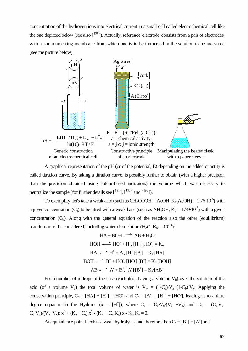
concentration of the hydrogen ions into electrical current in a small cell called electrochemical cell like

the one depicted below (see also [190]). Actually, reference 'electrode' consists from a pair of electrodes,

with a communicating membrane from which one is to be immersed in the solution to be measured

(see the picture below).

cork

pH

mV KCl(aq)

AgCl(pp)

Ag wires

- (RT/F)·ln(a(Cl-));E = E0

a = chemical activity; a = j·c; j = ionic strength F/RT)10ln(

EE)H/H(E 0−++

pH refref2

⋅−=

Generic construction

of an electrochemical cell Constructive principle

of an electrode Manipulating the heated flask

with a paper sleeve A graphical representation of the pH (or of the potential, E) depending on the added quantity is

called titration curve. By taking a titration curve, is possibly further to obtain (with a higher precision

ary to

OH, Ka(AcOH) = 1.76·10-5) with

he other (equilibrium)

actions must be considered, including water dissociation (H2O, Kw = 10-14):

BOH

than the precision obtained using colour-based indicators) the volume which was necess

neutralize the sample (for further details see [191], [192] and [193]).

To exemplify, let's take a weak acid (such as CH3COOH = Ac

a given concentration (Ca) to be titred with a weak base (such as NH4OH, Kb = 1.79·10-5) with a given

concentration (Cb). Along with the general equation of the reaction also t

re

HA + AB + H2O

HOH HO- + H+, [H+]·[HO-] = Kw

HA H+ + A-, [H+]·[A-] = Ka·[HA]

BOH B+ + HO-, [HO-]·[B+] = Kb·[BOH]

AB A- + B+, [A-]·[B+] = Ks·[AB]

For a number of n drops of the base (each drop having a volume Vb) over the solution of the

acid (of a volume Va) the total volume of water is Vw = (1-Ca)·Va+(1-Cb)·Vx. Applying the

conservation principle, Ca = [HA] + [H+] - [HO-] and Cs = [A-] – [H+] + [HO-], leading us to a third

degree equation in the Hydrons (x = [H+]), where Cs = Cb·Vx/(Va +Vx) and Cx = (Ca·Va-

Cb·Vx)/(Va+Vx): x3 + (Ka + Cs)·x2 - (Kw + Cx·Ka)·x - Kw·Ka = 0.

At equivalence point it exists a weak hydrolysis, and therefore then Cs = [B+] = [A-] and

62

x2 = )CK/()CK()K/KK( sasbbaw ++⋅⋅ , at equivalence point

Analogues, x3 + (Kw/Kb + x)·x2 - (Kw + Cs·Kw/Kb)·x - Kw2/Kb = 0, when the equilibrium point

is passed, where the expressions of Cx (base excess) and Cs are Cx = (Cb·Vx - Ca·Va)/(Va + Vx) and Cs =

Ca·Va/(Va+Vx). The thir

C

d degree equations can be solved and their roots (only one having a true

meaning, ranging in [0,1]) can be depicted as a function of the added volume. An online application

implementing this procedure of calculation is available (see [194] and papers [195] and [196]).

Other sensor-based applications include [197], [198], [199], [200], [201], [202] and [203] (see also

[204]).

The pH measurements (see [205], [206]; and in general, sensor based measurements, see for

instance [207]) have very important applications, ranging from environmental and biological ones to

industrial. An illustrative image about the pH of some common chemicals as well as natural products is

given in the next:

14 13 12 11 10 9 8 7 6 5 4 3 2 1 0

Battery acid

LemonVinegar

Baking soda

Mg(OH)2

Tomatoes

"Cola"Lime

BananasPotatoes

H3BO3

Adult fish die Fish reproduction affected

Acid rain

Stream water Normal range precipitation

Neutral

Increasing acidity

Increasing alkalinity

Sea water BloodCow milk

Urine

Adult fish die Juvenile fish die

-9.3 ~ HI HCl

NaOHKOH38 ~ KNH2

50°C NH4OHsat

0°C H2O2

Ca(OH)2

(1M)

(1M)

(1M)

Useful is also creation abas 8]) with equilibrium constants

of chemical reactions (see [209] 210])

of a dat e (for fast procedures, see [20

and [ .

63

Water analysis

ving more

substan

logical processes.

(H2O) essentially is nonexistent in the natural environment. Natural water, whether

in the atmosphere, on the ground surface, or under the ground, always contains dissolved minerals and

gases as a result of its interaction with the atmosphere, minerals in rocks, organic matter, and living

organisms. Some of the substances are miscible (mix in all proportions), others are hydrophilic (that is

attracted to and tends to be dissolved by water), others are soluble (depends on temperature, pressure

and the pH) while others are immiscible (incapable of mixing or attaining homogeneity).

Water purification is the process of removing undesirable chemicals, biological contaminants,

suspended solids and gases (for further details see [211], [212]). The goal of this process is to produce

water fit for a specific purpose. Most water is disinfected for human consumption (drinking water) but

water purification may also be designed for a variety of other purposes (meeting the requirements of

medical [213], pharmacological [214], chemical and industrial [215] applications). Purification includes

physical processes (filtration, sedimentation, and distillation), biological processes (using of slow sand

filters and biologically active carbon), chemical processes (flocculation and chlorination).

Water chemistry analyses are carried out to identify and quantify the chemical components and + + 2+ 2+ 2+ - - -

, unstable volatiles (CO2, H2S, O2) and isotopes ( O , H ),

organics and nutrients.

Purpose

It will be determined acidity, alkalinity and total hardness of the water.

Material and method

Samples of water will be analyzed in the laboratory and a bulletin of water analysis will be

obtained. In order to do this, samples of water will be taken from the tap and neutralization reactions

Introduction

In its liquid state, water forms the world's streams, rivers, lakes, oceans and rain and is the

major constituent of the fluids of living things, its percent in the human body ranging from 50% to

80%.

Water is a good polar solvent (often referred as the universal solvent) dissol

ces in greater quantities than any other common liquid being important in chemical, physical,

and bio

Sources of water include fresh water (from streams), salt water (from rivers and lakes),

seawater (from seas and oceans) as well as icebergs (in the polar region) and glaciers (at upper altitudes

in mountains).

Pure water

properties including pH, major cations (Na , K , Ca , Mg , Ba ) and anions (Cl , F , SO4 ,NO3 ),

trace elements (Rb+, Ti4+, Fe2+, Mn2+, etc.) 18 2- 2 +

2-

64

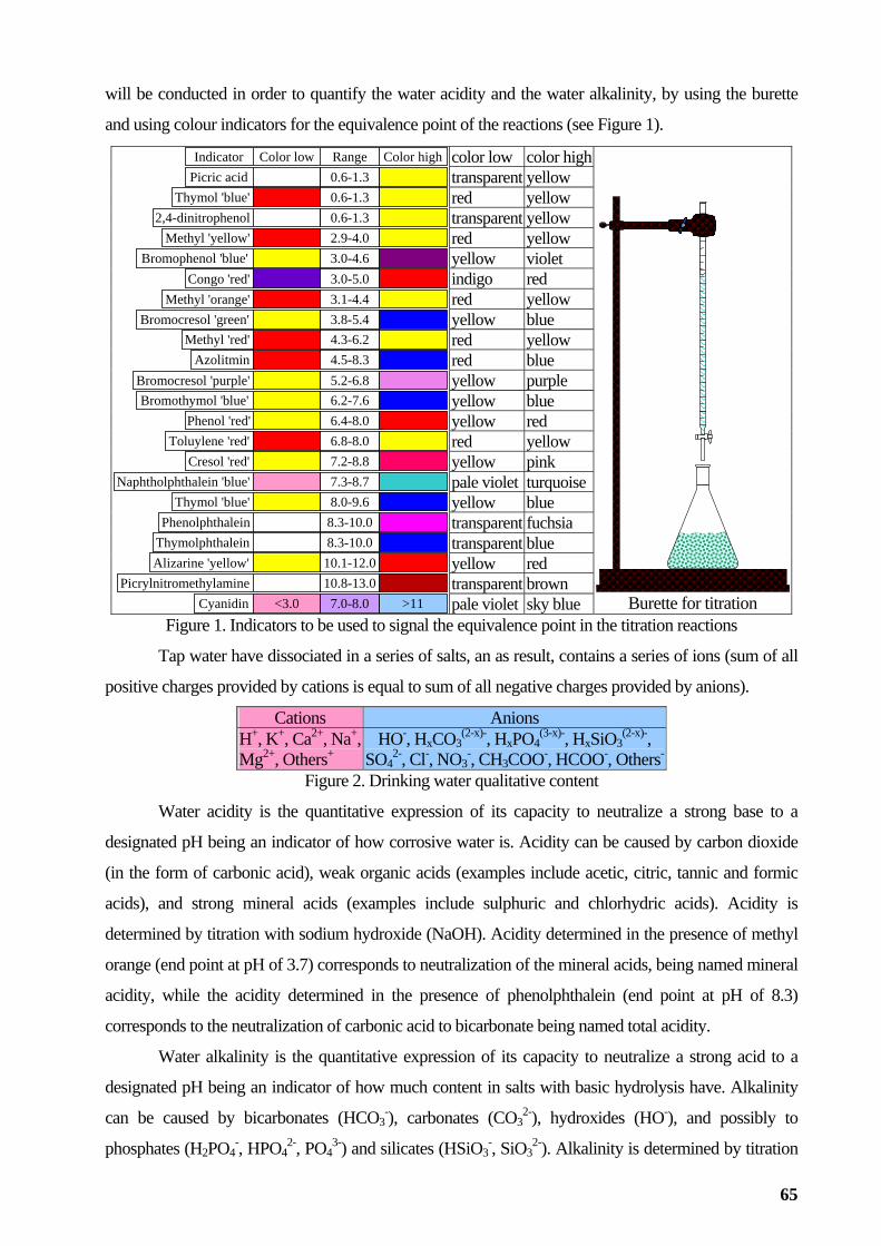
will be conducted in order to quantify th he water alkalinity, by using the burette

ivalence point of the reactions (see Figure 1).

e water acidity and t

and using colour indicators for the equ

color low color hightransparent yellow red yellow transparent yellow

Indicator Range Color low Picric acid

Color high0.6-1.3

Thymol 'blue' 0.6-1.3

red yellow yellow violet indigo red red yellow yellow blue red yellow red blue yellow purple yellow blue yellow red red yellow yellow pink pale violet turquoiseyellow blue transparent fuchsia transparent blue yellow red transparent brown

2,4-dinitrophenol 0.6-1.3 Methyl 'yellow' 2.9-4.0

omophenol 'blue' 3.0-4.6 Congo 'red' 3.0-5.0

Methyl 'orange'

Br

3.1-4.4 Bromocresol 'green' 3.8-5.4

Methyl 'red' 4.3-6.2 Azolitmin 4.5-8.3

Bromocresol 'purple' 5.2-6.8 Bromothymol 'blue' 6.2-7.6

Phenol 'red' 6.4-8.0 Toluylene 'red' 6.8-8.0

Cresol 'red' 7.2-8.8

Thymol 'blue' 8.0-9.6 Naphtholphthalein 'blue' 7.3-8.7

Phenolphthalein 8.3-10.0 Thymolphthalein 8.3-10.0 Alizarine 'yellow' 10.1-12.0

Picrylnitromethylamine 10.8-13.0Cyanidin >11 <3.0 7.0-8.0 Burette for titration pale violet sky blue

Figure 1. Indicators to be used to signal the equivalence point in the titration reactions

Tap water have dissociated in a series of salts result, contains a series of ions (sum of all

positive charges provided by cations is equal to sum of all negative charges provided by anions).

, an as

Cations Anions H+, K+, Ca2+, Na+, Mg2+, Others+

HO-, HxCO3(2-x)-, HxPO4

(3-x)-, HxSiO3(2-x)-,

SO42-, Cl-, NO3

-, CH3COO , HCOO-, Others- -

Figure 2. Drinking water qualitative content

Water acidity is the quantitative expression of its capacity to neutralize a strong base to a

a (

with sodium hydroxide (NaOH). Acidity determined in the presence of methyl

range (end point at pH of 3.7) corresponds to neutralization of the mineral acids, being named mineral

ined in the presence of phenolphthalein (end point at pH of 8.3)

tal acidity.

Water alkalinity is the quantitative expression of its capacity to neutralize a strong acid to a

content in salts with basic hydrolysis have. Alkalinity

designated pH being an indicator of how corrosive water is. Acidity can be caused by carbon dioxide

(in the form of carbonic acid), weak organic acids (examples include acetic, citric, tannic and formic

acids), and strong mineral cids examples include sulphuric and chlorhydric acids). Acidity is

determined by titration

o

acidity, while the acidity determ

corresponds to the neutralization of carbonic acid to bicarbonate being named to

designated pH being an indicator of how much

can be caused by bicarbonates (HCO3-), carbonates (CO3

2-), hydroxides (HO-), and possibly to

phosphates (H2PO4-, HPO4

2-, PO43-) and silicates (HSiO3

-, SiO32-). Alkalinity is determined by titration

65

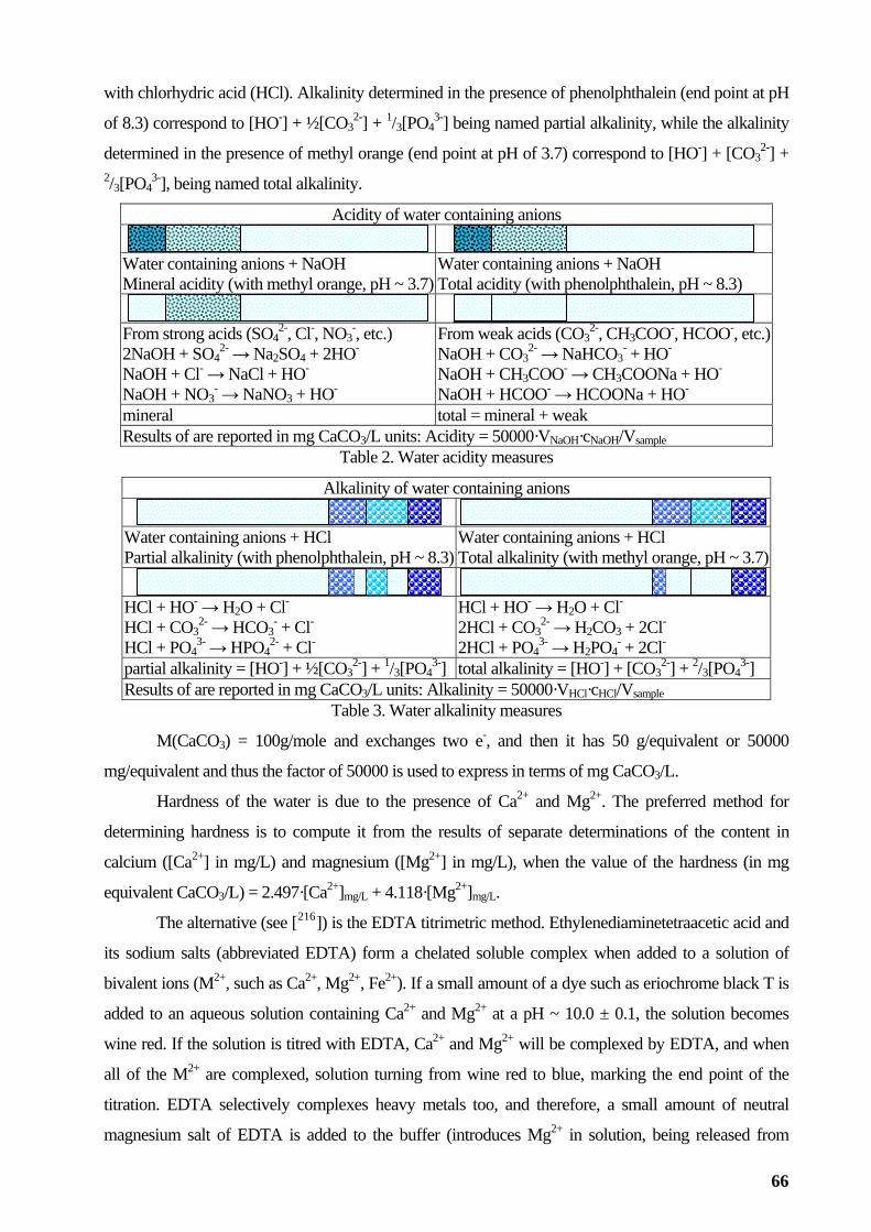
with chlorhydric acid (HCl). Alkalinity determined in the presence of phenolphthalein (end point at pH

of 8.3) correspond to [HO-] + ½[CO32-] + 1/3[PO4

3-] being named partial alkalinity, while the alkalinity

determined in the presence of methyl orange (end point at pH of 3.7) correspond to [HO-] + [CO32-] +

2/3[PO43-], being named total alkalinity.

Acidity of water containing anions

Water containing anions + NaOH Mineral acidity (with methyl orange, pH ~ 3.7)

Water containing anions + NaOH T lphthalein, pH ~ 8.3) otal acidity (with pheno

From strong acids (SO42-, Cl-, NO3

-, etc.) 2NaOH + SO4

2- → Na2SO4 + 2HO- NaOH + Cl- → NaCl + HO- NaOH + NO3

- → NaNO3 + HO-

F weak acids (CO32-, CH3COO-, HCOO-, etc.)

NaOH + CO NaHCO3- + HO-

NaOH + CH → CH3COONa + HO- NaOH + HC → HCOONa + HO-

rom32- →

3COO-

OO- mineral t ineral + weak otal = mResults of are reported in mg CaCO3/L units: Ac = 500 H·cNaOH/Vsample idity 00·VNaO

Table 2. Water acidity measures

Alkalinity of wate gr containin anions

Water containing anions + HCl Partial alkalinity (with phenolphthalein, pH ~ 8.3

ng anions + HCl alk y (with methyl orange, pH ~ 3.7)) Total

Water containialinit

HCl + - -

HCl +HCl

HO → H2O + Cl CO3

2- → HCO3- + Cl-

HCl + HO → H2O + Cl 2HCl + CO3

2- → H2CO3 + 2Cl- - -

+ PO43- → HPO4

2- + Cl- 2HCl + PO43- → H2PO4

- + 2Cl- partial alkalinity = [HO-] + ½[CO3

2-] + 1/3[PO43-] total alkalinity = [HO-] + [CO3

2-] + 2/3[PO43-]

Results of are reported in mg CaCO /L units: Alkalinity = 50000·V ·c /V 3 HCl HCl sampleTable 3. Water alkalini res

M(CaCO3) uivalent or 50000

mg/equivalent and thus the fa g CaCO3/L.

n becomes

ty measu

= 100g/mole and exchanges two e , nd then it has 50 g/eq- a

ctor of 50000 is used to express in terms of m

Hardness of the water is due to the presence of Ca2+ and Mg2+. The preferred method for

determining hardness is to compute it from the results of separate determinations of the content in

calcium ([Ca2+] in mg/L) and magnesium ([Mg2+] in mg/L), when the value of the hardness (in mg

equivalent CaCO3/L) = 2.497·[Ca2+]mg/L + 4.118·[Mg2+]mg/L.

The alternative (see [216]) is the EDTA titrimetric method. Ethylenediaminetetraacetic acid and

its sodium salts (abbreviated EDTA) form a chelated soluble complex when added to a solution of

bivalent ions (M2+, such as Ca2+, Mg2+, Fe2+). If a small amount of a dye such as eriochrome black T is

added to an aqueous solution containing Ca2+ and Mg2+ at a pH ~ 10.0 ± 0.1, the solutio

wine red. If the solution is titred with EDTA, Ca2+ and Mg2+ will be complexed by EDTA, and when

all of the M2+ are complexed, solution turning from wine red to blue, marking the end point of the

titration. EDTA selectively complexes heavy metals too, and therefore, a small amount of neutral

magnesium salt of EDTA is added to the buffer (introduces Mg2+ in solution, being released from

66

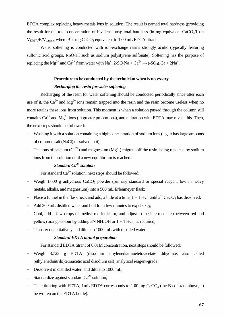
EDTA complex replacing heavy metals ions in solution. The result is named total hardness (providing

the result for the total concentration of bivalent ions): total hardness (in mg equivalent CaCO3/L) =

VEDTA·B/Vsample, where B is mg CaCO3 equivalent to 1.00 mL EDTA titrant.

Water softening is conducted with ion-exchange resins strongly acidic (typically featuring

sulfonic acid groups, RSO3H, su ). Softening has the purpose of

replacing the Mg2+ and Ca2+ from water with Na+: 2-SO3Na + Ca2+ → (-SO3)2Ca + 2Na+.

Procedure to be conducted by the technician when is necessary

ter so

er softeni fter each

us ain trapped less when no

mo sse rou h the column still

contains Ca and Mg ions (in gr ith EDTA may reveal this. Then,

the next steps should be followed

÷ Washing it with a solution containing a high concentration of sodium ions (e.g. it has large amounts

÷ The ions of calcium (Ca2+) and magnesium (Mg2+) migrate off the resin, being replaced by sodium

til new equilibrium is r

Standard lution

÷ heavy

as dissolved;

Add

ed water.

ch as sodium polystyrene sulfonate

Recharging the resin for wa ftening

Recharging of the resin for wat ng should be onducted pe iodically since ac r

e of it, the Ca2+ and Mg2+ ions rem into the resin and the resin become use

re retains these ions from solution. This moment is when a solu pa d th g2+ 2+

tion

eater proportions), and a titration w

:

of common salt (NaCl) dissolved in it);

ions from the solution un a2+

eached.

Ca so

For standard Ca2+ solution, next steps should be followed:

Weigh 1.000 g anhydrous C r special reagent low inaCO3 powder (primary standard o

metals, alkalis, and magnesium) into a 500 mL Erlenmeyer flask;

÷ Place a funnel in the flask neck and add, a little at a time, 1 + 1 HCl until all CaCO3 h

÷ 200 mL distilled water and boil for a few minutes to expel CO2;

÷ Cool, add a few drops of methyl red indicator, and adjust to the intermediate (between red and

yellow) orange colour by adding 3N NH4OH or 1 + 1 HCl, as required;

÷ Transfer quantitatively and dilute to 1000 mL with distill

Standard EDTA titrant preparation

For standard EDTA titrant of 0.01M concentration, next steps should be followed:

÷ Weigh 3.723 g EDTA (disodium ethylenediaminetetraacetate dihydrate, also called

(ethylenedinitrilo)tetraacetic acid disodium salt) analytical reagent-grade;

÷ Dissolve it in distilled water, and dilute to 1000 mL;

÷ Standardize against standard Ca2+ solution;

÷ Then titrating with EDTA, 1mL EDTA corresponds to 1.00 mg CaCO3 (the B constant above, to

be written on the EDTA bottle).

67

Working procedure

Acidity and alkalinity of water

For mineral acidity follow the next steps (for two samples of about 100 ml of water from tap):

In a

Titrate with NaOH the water sample till the moment in which a colour change is observed;

Rec rd the

tota ity' replacing 'methyl orange indicator' with

ndicator Vinitial Vfinal (Vfinal-Vinitial)/Vi Average((Vfinal-Vinitial)/Vi)

÷ n Erlenmeyer flask (of about 300 ml) take a sample of water; record its volume (Vj);

÷ Add a drop of methyl orange indicator;

÷ Record the volume of NaOH from the burette (Vinitial) in the table below;

÷

÷ o volume of NaOH from the burette (Vfinal) in the table below;

For l acidity repeat the steps from 'mineral acid

'phenolphthalein indicator'.

For total alkalinity repeat the steps from 'mineral acidity' replacing 'NaOH' with 'HCl'.

For permanent alkalinity repeat the steps from 'mineral acidity' replacing 'NaOH' with 'HCl' and

'methyl orange indicator' with 'phenolphthalein indicator'.

Analysis Water (ml) Titrant IV1 = mineral

acidity V2 = NaOH methyl orange a1 = V3 = total

acidity V4 = NaOH phenolphthalein a2 =

V5 = total alkalinity V6 = HCl methyl orange a3 =

V7 = partial HCl phenolphtalkalinity V8 = halein a4 =

Table 4. Acidity and alkalinity of water samples

e (Vj);

H of 10±0.1);

Ad );

nge is observed;

in the table below;

e resin column to collect two samples (see the figure)

Hardness and softening of water

For hardness follow the next steps (for two samples of about 100 ml of water from tap):

÷ In an Erlenmeyer flask (of about 300 ml) take a sample of water; record its volum

÷ Add HCl with 2 mL more than the average of (Vfinal-Vinitial) needed for mineral acidity;

÷ Boil the sample in the flask for 5 minutes;

÷ Add 2 ml NaOH;

÷ Add 2 ml buffer (NH4OH) solution (to provide a p

÷ d few crumbs of eriochrome black T indicator (till the solution become pale coloured

÷ Record the volume of EDTA from the burette (Vinitial) in the table below;

÷ Titrate with EDTA the water sample till the moment in which a colour cha

÷ Record the volume of EDTA from the burette (Vfinal)

For softening add water on the top of th

and then repeat the procedure measuring the hardness with the softened water, filling the values in the

next table (Table 4).

68

Hardness Water (ml) Titrant Indicator Vinitial Vfinal (Vfinal-Vinitial)/Vi Average((Vfinal-Vinitial)/Vi)V1 = regular V = 2 a5 =

V3 = softened EDTA eriochrome black T

a = V4 = 6

Table 4. Hardness of the regular and softened water

Resin column

e Titrating with

Heating th

Mfla burett e flask

anipulating the heatedsk with a paper sleeve

Figure 1. Conducting he e periments Data analy

- - CO32- as significant bases, then the amount of H+

- CO32-

t x

sis

If a water contains only HO , HCO3 and

required to reach the phenolphthalein endpoint is equal to the amount of HO plus the amount of+ -originally present (H + OH H2O; H + CO3 + 2- HCO3 , because at the pH = 8.3 where

-

-

phenolphthalein changes its colour most of the alkalinity will be in the form of HCO3 . Any rem- 2-

aining

HO or CO would be exactly balanced by an equivalent amount of CO2.

one must add an additional amount of H+ to the amount + + HCO -

3

To reach the methyl orange endpoint,

of HCO - present at the phenolphthalein endpoint: H H2CO3 CO2 + H2O. This

ent since carbonate was entirely

s can be

3 3

will be equal to the amount of HCO - plus CO 2- originally pres3 3

converted to bicarbonate in the first stage, and thus calculations of these species concentration

conducted (see Table 5).

Alkalinity If a3/a4 ≤ 2 If a3/a4 ≥ 2 from HO- 2·(partial alkalinity) - (total alkalinity) 0 from CO3 2·(total alkalinity - partial alkalinity) 2·(partial alkalinity) 2-

from HCO3- 0 total alkalinity - partial alkalinity

Table 5. Approximate calculations from alkalinity of the water

Thus, stating

from the experimental results (data from Table 4) calculations based on the

69

formulas given (Table 2, Table 3 5) sh

th is bulletin below (Table 6).

antit V lue Measu nt unit

and Table ould be conducted, and the results are to be written in

e water an lysa

Qu y a remeUsed solutions ÷ Concen itten tration of NaOH solution to be written to be wr÷ Concentration of HCl solution to be written to be written ÷ Concentration of EDTA solution to be written to be written Acidity and alkalinity ÷ Mineral acidity to be written mg CaCO3/L ÷ Total acidity to be written mg CaCO3/L ÷ Difference (weak acids) to be written mg CaCO3/L ÷ Partial alkalinity to be written mg CaCO3/L ÷ Total alkalinity to be written mg CaCO3/L ÷ Approximate alkalinity from HO- to be written mg CaCO3/L ÷ Approximate alkalinity from HCO3

- to be written mg CaCO3/L ÷ Approximate alkalinity from CO3

2- to be written mg CaCO3/L Hardness of the water ÷ Regular water to be written mg CaCO3/L ÷ Softened water to be written mg CaCO3/L

Table 6. Water analysis bulletin

Further reading

Complexometry

Complexometry (or ch on of metal complexes with

being improved method after 1940. During titration sample

s combines the advantages

cipi ors (like precipitation

ganic solvent, and therefore should pay attention to its solubility. Of these, the

most use e raacetic acid (EDTA), denoted symbolically H4Y (namely the

disodium tructural formula in

figure 2, along with logarithms of solubility constants for ED s. EDTA

have 6 acidity const 6.16, and pKa4 =

elatometry) is based on the formati

polycarboxylic acids and polyamines

solution forms a stoechiometric complex soluble and undissociated. Techniques by which this

operation is conducted are typical volumetric titration procedures. The general method has three main

aspects: the choice of a suitable chelating agent, the choice of experimental conditions titration gives

optimum (checking the pH and the presence of competitive ligands) and the choice of an appropriate

method for the detection of the equivalence point. Complexation titration

and disadvantages of methods of titration in general and the formation of complexes: reaction product

(complex) is undissociated, the complex does not give copre tation err

titrations), it have selectivity: complexing agent coordinates only certain metal ions, while the

stoichiometry is not as well defined as in the titration of the precipitation, neutralization, or redox, if the

complexing agent is an or

d is ethyl nediaminetet

salt of the acid, which is soluble in water denoted H2YNa2), with the s

TA complexes of some metal ion

ants, pKa-2 = 0.0, pKa-1 = 1.5, pKa1 = 2.0, pKa2 = 2.66, pKa3 =

10.24. This combination is known also under the name of Complexone III. It has the ability to form

70

stable complexes, called complexones, with a large number of metals (Ca, Mg, Zn, Cd, Pb, Cu, Ni, Fe,

etc.). These complexes are closing cycles (in this case of 5 atoms), and the chelating complexes are

known to be very stable, but not coloured. Complex is wide l analysis to

determine the

Group 1

one III ly used in chemica

displacement of many metals, by complexometric titration.

Group 2 Group 3Mg 8.69 Mn 13.58 Hg 21.8 Ca 10.7 Fe 14.33 Bi 23 Sr o 36 8.63 Rare earths 15.3-19.8 CBa 7.76 Cr 23 Co 16.21

Ni 18.56 Fe 25.1 Cu 18.79 Ga 20.27Zn 16.5 In 24.95Cd 16.59 Sc 23.1 Al 16.13 Sn 22 Pb 18.3 Ti 17.7 TiO 17.3 Tl 23.2 V 12.7 25.9 V

VO 18.77

N

N

OH

OH

NaOOC

C

CH2

NaOO CH2O

O

N

N

O

O

ONa

ONa

O

OO

O

Ca

H2YNa (2 o

Ca bivalent metal)

di-sodium salt f EDTA) and YNa (or M, a2

Figure 2. Solubilities of the EDTA complexes by analytical groups of

An alternative is conducting previously a qualitative analysis, which may have the purpose of

stance [217] and [218]). Other preliminary studies may include

], [222], [223], [224], [225], [226], [227] and [228]).

cations (expressed in pKa units)

the increasing of the sensitivity (see for in

the molecular design (see [219], [220], [221

In order to indicate the equivalence point in complexometric titration, complexometric

indicators are used. They are organic materials which form coloured complexes with metal ions, less

stable than those of the respective metal complexone III. During titration with EDTA solution, which

remove metal ions complex with the indicator, are formed the complexone which is more stable. At the

end of the titration, at the equivalence point, the total amount of metal present in the sample is bound in

the form of complexone (colourless), and the colour of the indicator solution appears clear. Most are

using eriochrome black T complexometric indicators and murexide. Because EDTA is an acid, the pH

depends on the stability of its complexes. Thus, in strongly acidic solution, the complex tends to release

the metallic ion and reforming acid EDTA. Therefore complexometric titration is carried out in basic

medium (in the presence of a basic buffer solution).

Species responsible for alkalinity and acidity in waters

Alkalinity and acidity can be interpreted in terms of concentrations of specific constituents

only when the chemical composition of the water is known (this being the 'ideal' case). The species that

provide alkalinity to water are bases and the species that provide acidity to water are acids. In

unpolluted fresh waters, hydroxide, carbonate and bicarbonate are the most important bases. Therefore,

total alkalinity is often approximated as the sum of the number of equivalents of these bases (minus the

71

hydrogen ion concentration):

Total alkalinity ~ [HCO3-] + 2·[CO3

2-] + [HO-] - [H+]

In rare cases other bases may also be important such as the silicates, ammonia, phosphates,

borates and organic bases. For example, extremely soft waters (total alkalinity < 10 mg CaCO3/L)

contain so little bicarbonate that ammonia and silicate concentrations become important. Aside from

H+ anion d i aters in order of importance are the carbonates, sulphate,

ch fluoride, boron, bromide, ammonia and phosphate. Of these,

sulphate, chloride, nitrate, fluori romide are insufficiently basic to contribute to alkalinity

regardless eir con ion y, most of the major cations such as calcium, sodium,

magnesium assium tron ot hydrolyze to a sufficient extent within the pH range of

interest to a nt for m kal the remaining species of interest are listed in the next table

(Table 7), a with th mon m oncentration (c, in moles/L).

Specie c

and OH-, the s foun n fresh w

loride, silicate, organic anions, nitrate,

de and b

of th centrat . Similarl

, pot and s tium do n

ccou uch al inity, and

long eir com olar c

s Ref pKa Equilibrium 10.3 CO3

2- + 2H+ HC +O3 + H -Carbonates 1·10 [229] -

-36.4 HCO3 + H+ H2CO3

Silicates 2·10-4 [230] 9.8 H SiO + H+ H SiO 3 4 4 4Organics 1·10-4 [231] 3-10 R-COO- + H+ R-COOH Borates 1·10-6 [232] 9.2 B(OH)4

- + H+ B(OH)3 + H2O

Ammonia 2·10-6 [233] 9.2 NH4OH + H+ NH4+ + H2O

Iron 6.0 Fe(OH)4- + 2H+ Fe(OH)2

+ + 2H2O

2·10-6 [234] 4.6 Fe(OH) +2 + + H 2+ + H O Fe(OH) 2

8.0 Al(OH)4- + H+ Al(OH)3 + H2O

5.7 Al(OH)3 + H+ Al(OH)2+ + H2O

4.3 Al(OH)2+

+ H+ Al(OH)2+ + H2O Aluminium 2·10-6 [235]

5.0 Al(OH)2+ + H+ Al3+ + H2O 12.3 PO4

3- + H+ HPO42-

7.2 HPO42- + H+ H2PO4

- Phosphates 7·10-7 [236]2.1 H2PO4

- + H+ H3PO4 Hydroxide 2·10-7 [237] 14.0 OH- + H+ = H2O

9.8 Cu(OH)3- + 2H+ Cu(OH)+ + 2H2O Copper 1·10-7 [238] 7.3 Cu(OH)++ H+ Cu2+ + H2O

Nickel 2·10-8 [239] 6.9 Ni(OH)2 + H+ Ni(OH)+ Cadmium 1·10-8 [240] 7.6 Cd(OH)+ + H+ Cd+2 + H2O Lead 1·10-8 [241] 6.2 Pb(OH)+ + H+ Pb+2 + H O 2

19.0 S2- + H+ HS- Sulphides 2·10-5 [242] 7.0 HS- + H+ H2S

6.1 Zn(OH)2 + H + Zn(OH)+ + H2O Zinc 8·10-7 [243] 9.0 Zn(OH)+ + H+ Zn2+ + H2O Table 7. Species which contribute to the alkalinity of drinking waters

Based on the average concentrations shown here, the practice of interpreting fresh water

alkalinity in terms of the carbonate system is justified. It is important to point out here that although

carbonates contribute to alkalinity, the addition of carbon dioxide to water will not alter its alkalinity,

because carbon dioxide consumes one hydroxide molecule for each bicarbonate molecule formed.

72

CO2(aq) + OH- → HCO3-

The addition or loss of ca .

In

rbon dioxide might, however, result in a change in pH

contrast to fresh waters, seawater has such high concentrations of other bases, when the total

alkalinity is usually expressed as:

Total alkalinity = [HCO3-] + 2·[CO3

2-] + [B(OH)4] + [HPO42-] + [H3SiO4] + [Mg(OH)-] + [OH-] - [H+]

In industry, special processes may be involved for removing of specific compounds from

aqueous and gaseous phase (see [56] and [57]) while environmental monitoring requires complex

analysis involving the identification of the mechanisms (see [244]).

73

Volumetric and gravimetric methods in study of corrosion

truction of materials by chemical reaction with substances from their

e

is con

cing oxide(s) or salt(s) of the metal.

Rusting (the formation of iron oxides) is a well-known example of corrosion.

Many alloys corrode merely from exposure to moisture in air, and the process can be strongly

affected by the presence of certain substances. Corrosion can occur locally to form a pit or crack, or it

can extend across a wide (more or less uniformly) area at the surface (occurs on exposed surfaces being

a diffusion-controlled process).

There are several methods to reduce the chemical activity at the exposed surface, such as

passivation and electroplating.

Passivation involves a shielding outer-layer of base material, which can be applied as a

microcoating, or which occurs spontaneously in nature. As a technique, passivation is the use of a light

coat of a protective material, such as metal oxide, to create a shell against corrosion.

Electroplating is a process that uses electric current to reduce dissolved metal cations so that

they form a coherent metal or alloy coating on a metal surface acting as an electrode. Electroplating is

widely used in various industries for coating metal or alloy objects with a thin layer of a different metal

or alloy or with a different composition of the same alloy. Anyway, the purpose is the same, to increase

a material's corrosion resistance. Chromating is used for aluminium, zinc, cadmium, copper, silver,

magnesium, and tin alloys while nickeling (nickel deposition) and galvanization (zinc deposition) is

mainly used for iron alloys. Other alternatives are to do electroplate with an alloy (see [245]).

Gravimetric analysis is defined as the quantitative determination of quantities based on weight

difference and eventually based on correspondences from chemical reactions. Mass is the most

fundamental of all analytical measurements, and gravimetry is the oldest quantitative technique.

Similarly, volumetric analysis is defines as the quantitative determination of quantities based on

volume difference eventually based on correspondences from chemical reactions.

In both gravimetry and volumetry measurements can be conducted in all aggregation states

(solid, liquid, gaseous) but in general are preferred solid state for gravimetry and liquid or gaseous state

for volumetry. Both methods are chemical methods, meaning that the analysis is based on a change in

the substance due to a chemical reaction and the measurements are conducted in absolute units (of

mass and of volume).

Introduction

Corrosion is a gradual des

nvironment. Corrosion can occur in materials other than metals (such as ceramics or polymers), but in

th text, the term degradation is more common.

Therefore, in the most common sense used, corrosion means electrochemical oxidation of

metals in reaction with an oxidant (such as oxygen), typically produ

74

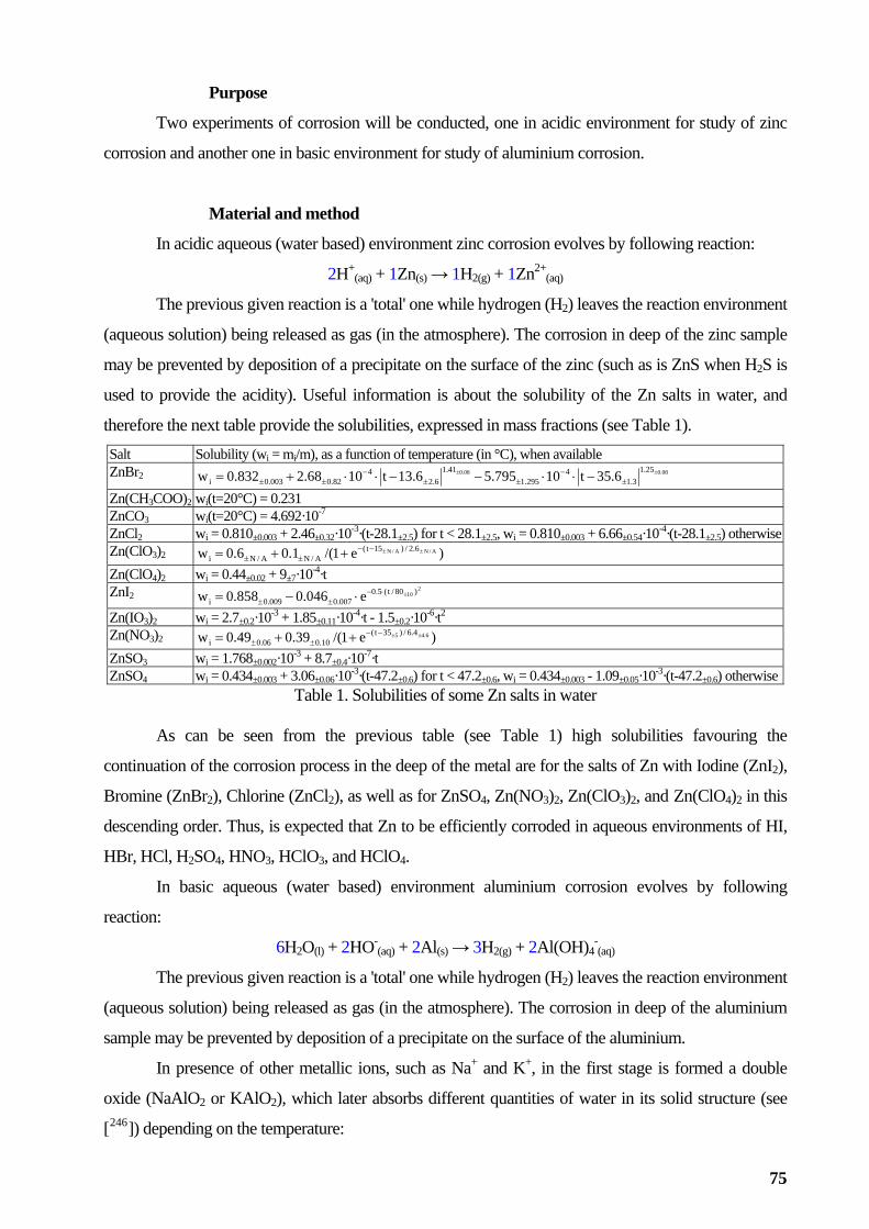
Two experiments of corrosion will be conducted, one in acidic environment for study of zinc

ironment for study of aluminium corrosion.

deep of the zinc sample

ay be

as a function of temperature (in °C), when available

Purpose

corrosion and another one in basic env

Material and method

In acidic aqueous (water based) environment zinc corrosion evolves by following reaction:

2H+(aq) + 1Zn(s) → 1H2(g) + 1Zn2+

(aq)

The previous given reaction is a 'total' one while hydrogen (H2) leaves the reaction environment

(aqueous solution) being released as gas (in the atmosphere). The corrosion in

m prevented by deposition of a precipitate on the surface of the zinc (such as is ZnS when H2S is

used to provide the acidity). Useful information is about the solubility of the Zn salts in water, and

therefore the next table provide the solubilities, expressed in mass fractions (see Table 1). Salt Solubility (wi = mi/m),ZnBr2 08.008.0 25.1441.14 ±± −− −⋅⋅−−⋅⋅

3.1295.16.282.0003.0i 6.35t10795.56.13t1068.2832.0w ±±±±± +=

Zn(C COO)2 wi(t=20°C) = 0.231 H3ZnCO3 wi(t=20°C) = 4.692·10-7 ZnCl w = 0.810 + 2.462 ·10-3·(t-28.1 ) for t < 28.1 , w = 0.810 + 6.66 ·10-4·(t-28.1 ) otherwisei ±0.003 ±0.32 ±2.5 ±2.5 i ±0.003 ±0.54 ±2.5Z 3)2 )e1/(1.06.0w A/NA/N 6.2/)15t(

A/NA/Ni±±−−

±± ++= n(ClOZn(ClO4)2 wi = 0.44±0.02 + 9±7·10-4·t ZnI2 2

10 )80/t(5.0007.0009.0i e046.0858.0w ±⋅−

±± ⋅−= Zn(IO3)2 wi = 2.7±0.2·10-3 + 1.85±0.11·10-4·t - 1.5±0.2·10-6·t2

Zn(NO )2 )e1/(39.049.0w 6.45 4.6/)35t(10.006.0i

±±−−±± ++= 3

ZnSO3 wi = 1.768±0.002·10-3 + 8.7±0.4·10-7·t ZnSO4 wi = 0.434±0.003 + 3.06±0.06·10-3·(t-47.2±0.6) for t < 47.2±0.6, wi = 0.434±0.003 - 1.09±0.05·10-3·(t-47.2±0.6) otherwise

Table 1. Solubilities of some Zn salts in water As can be seen from the previous table (see Table 1) high solubilities favouring the

continuation of the corrosion process in the deep of the metal are for the salts of Zn with Iodine (ZnI2),

Bromine (ZnBr2), Chlorine (ZnCl2), as well as for ZnSO4, Zn(NO3)2, Zn(ClO3)2, and Zn(ClO4)2 in this

descending order. Thus, is expected that Zn to be efficiently corroded in aqueous environments of HI,

eaction environment

temperature:

HBr, HCl, H2SO4, HNO3, HClO3, and HClO4.

In basic aqueous (water based) environment aluminium corrosion evolves by following

reaction:

6H2O(l) + 2HO-(aq) + 2Al(s) → 3H2(g) + 2Al(OH)4

-(aq)

The previous given reaction is a 'total' one while hydrogen (H2) leaves the r

(aqueous solution) being released as gas (in the atmosphere). The corrosion in deep of the aluminium

sample may be prevented by deposition of a precipitate on the surface of the aluminium.

In presence of other metallic ions, such as Na+ and K+, in the first stage is formed a double

oxide (NaAlO2 or KAlO2), which later absorbs different quantities of water in its solid structure (see

[246]) depending on the

75

2Al + 2NaOH(aq) + 2H2O(l) → 2NaAlO2(s) + 3H2(g)

The experimental apparatus for zinc corrosion is assembled and the experiment is conducted as

2NaAlO2 + 3H2O → 2NaAlO2·3/2H2O at 5-45°C

4NaAlO2 + 5H2O → 4NaAlO2·5/4H2O at 60-140°C

is illustrated below (see Figure 1).

Experimental apparatus before using for corrosion Experimental apparatus during use for corrosion

Starting the chronometer for corrosion of Zn Stopping the chronometer for corrosion of Zn

Figure 1. Study o

Vi

Vf

f the corrosion of zinc by volumetric method

76

The experimental and the experiment is

conducted as is illustrated b

apparatus for aluminium corrosion is assembled

elow (see Figure 2).

Figure 2. Study of the corrosion of aluminium by gravimetric method

Working procedure

Corrosion of zinc

The succession of the steps is as follows (data to be filled in Table 2):

÷ Take the sample, polish (with abrasive paper) and degreases it (with limewater, Ca(OH)2) if is

necessary;

÷ Measure the surface of the sample (by using the ruler) and record the value (S);

÷ Open the corrosion vessel, fix the sample in its support and put the cork assuring that no air is

allowed to pass in the vessel;

÷ Open the valve to allow the liquid to pass out from the vessel and to pass in the burette;

÷ Wait a little time till the liquid flows with constant speed;

id

÷ After a while, in the same moment record the level of the liquid in the burette (Vf = V2) and stop

the timer (t2);

÷ Close the valve which allow the liquid to pass out from the vessel;

÷ Remove the sample from the vessel by taking the cork with which the sample is connected.

S Vi = V1 Vf = V2 ΔV Δt = t2 - t1

÷ In the same moment, record the level of the liqu in the burette (Vi = V1) and start the timer (t1);

cm2 ml ml ml s

Table 2. Experimental data from corrosion of zinc

Corrosion of aluminium

The succession of the steps is as follows (data to be filled in Table 3):

÷ Take the sample, polish (with abrasive paper) and degreases it (with limewater, Ca(OH)2) if is

necessary;

÷ Measure the surface of the sample (by using the ruler) and record the value (S);

÷ Weight the sample using the analytical balance and record the value (m1);

÷ Fix the sample in its support, place it into the corrosion vessel and start the timer (t1);

77

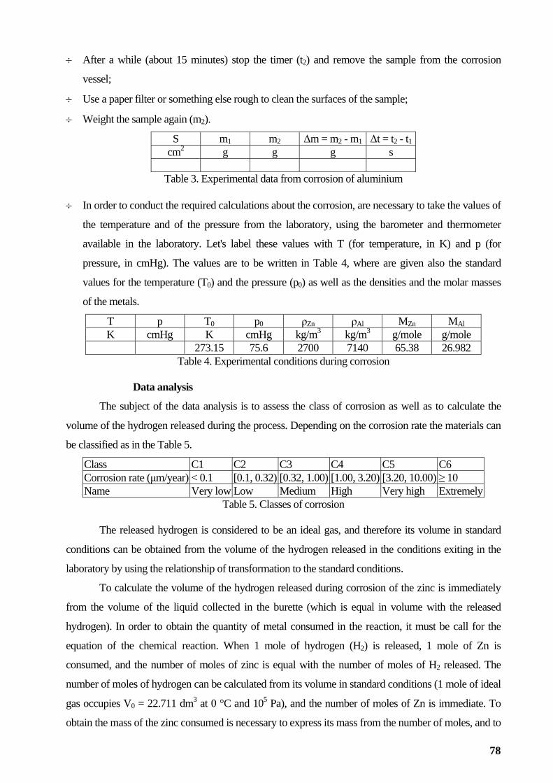
÷ er a while (about 15 minutes) stop the timer (t2) and remove the sample from the corrosion

vessel;

Aft

÷ Use a paper filter or something else rough to clean the surfaces of the sample;

÷ Weight the sample again (m2).

S m1 m2 Δm = m2 - m1 Δt = t2 - t1 cm2 g g g s

Table 3. Experimental data from corrosion of aluminium

In order to co ke the values of

the laboratory, using the barometer and thermometer

el these values with T (for temperature, in K) and p (for

pre given also the standard

s.

MAl

nduct the required calculations about the corrosion, are necessary to ta÷

the temperature and of the pressure from

available in the laboratory. Let's lab

ssure, in cmHg). The values are to be written in Table 4, where are

values for the temperature (T0) and the pressure (p0) as well as the densities and the molar masses

of the metal

T p T0 p0 ρZn ρAl MZn K cmHg K cmHg kg/m3 kg/m3 g/mole g/mole

273.15 75.6 2700 7140 65.38 26.982 Table 4

. Experimental conditions during corrosion

of corrosion as well as to calculate the

n

C1 C2 C3 C4 C5 C6

Data analysis

The subject of the data analysis is to assess the class

volume of the hydrogen released during the process. Depending on the corrosion rate the materials ca

be classified as in the Table 5.

Class Corrosion rate (μm/year) < 0.1 [0.1, 0.32) [0.32, 1.00) [1.00, 3.20) [3.20, 10.00) ≥ 10 Name Very low Low Medium High Very high Extremely

Table 5. Classes of corrosion The released hydro n is c to e in standard

conditions can be obtained from the volume of the hydrogen in the conditions exiting in the

laboratory by using the rel s .

r eased during corrosion of the zinc is immediately

om th olume with the released

ical reaction. When 1 mole of hydrogen (H2) is released, 1 mole of Zn is

f H2 released. The

nditions (1 mole of ideal

mediate. To

obtain the mass of the zinc consumed is necessary to express its mass from the number of moles, and to

ge onsidered be an ideal gas, and therefore its volum

released

ationship of transformation to the standard condition

To calculate the volume of the hydrogen el

fr e volume of the liquid collected in the burette (which is equal in v

hydrogen). In order to obtain the quantity of metal consumed in the reaction, it must be call for the

equation of the chem

consumed, and the number of moles of zinc is equal with the number of moles o

number of moles of hydrogen can be calculated from its volume in standard co3 5gas occupies V0 = 22.711 dm at 0 °C and 10 Pa), and the number of moles of Zn is im

78

obtain its volume is necessary to use the density.

To calculate the volume of the hydrogen released during corrosion of the aluminium is

ed in the reaction, by

ical reaction. When 3 moles of hydrogen (H2) are released, 2 moles

of Al are consumed. The umber of moles of hydroge e in standard

conditions (1 mole of ideal gas occupies V0 = 22.711 dm3 at 0 and 105 P the number of moles of

Al being immediate fr sumed is necessary to

express its volume by using the density.

necessary to calculate first its number of moles from the quantity of metal consum

calling for the equation of the chem

n n can be used to obtain its volum

°C a),

om its mass. To obtain the volume of the aluminium con

The volume divided by the surface provides the penetration deep. In order to obtain the

corrosion rate by year, this penetration deep should be divided by the corrosion time (in s) and

multiplied with the number of seconds in 365 days (31536000 s).

Following table is to be filled (Table 6) for corrosion of Zn.

Parameter Measure Unit Value Calculation hint Surface S cm2 from Table 2 Corrosion time Δt s from Table 2 Volume of H2 2) ml f ble ΔV(H rom Ta 2 Standard volume 2 VSTD

3 Δ ΔV 0/T of H Δ (H2) dm VSTD = ·(p/p0)·(T ) Num er of moles of H2 Δ 0 0 0b n(H2) moles Δn = ΔV·(p/p )·(T /T)/V Number of moles of Zn Δn(Zn) moles (aq) (s) → 1H2(g) + 1Zn2+

(aq) 2H+ + 1ZnMass of Zn corroded Δm(Zn) g Δm = Δn·M Volum of Zn corroded ΔV(Zn) m ΔV = Δm/ρ e 3

P tion deep in Zn Δh(Zn) m Δh = ΔV/S enetraPenetration rate v(Zn) μm/year v = Δh/Δt Resistance class of Zn C1-C6 from Table 5

Table 6. Calculations for the corrosion of Zn

d (T

Par Mea

Following table is to be fille able 7) for corrosion of Al.

ameter sure Unit Valu ioe Calculat n hint Surface S cm2 from Table 2 C ion time Δt s from Table 2 orrosM f Al corroded Δm(Al) g from Table 2 ass oNumber of moles of Al Δn(Al) moles Δn = Δm/M Number of moles of H2 Δn(H2) moles 2Al + 2NaOH(aq) + 2H2O(l) → 2NaAlO2(s) + 3H2(g)Standard volume of H ΔV (H ) dm3 ΔV = Δn·V2 STD 2 STD 0 Volu e of H2 ΔV(H2) ml ΔV = ΔVSTD·(p0/p)·(T/T0) mVolume of Al corroded ΔV(Al) m3 ΔV = Δm/ρ Penetration deep in Al Δh(Al) m Δh = ΔV/S Penetration rate v(Al) μm/year v = Δh/Δt Resistance class of Al C1-C6 from Table 5

Table 7. Calculations for the corrosion of Al

79

Nickel corrosion protective electroplating

is supplied with electrons to form a non-ionic coating on a

ally, a cathode (negatively charged)

ome plating h at ing the electrolytic deposition of chromium. The

rm of chrome plati is the in, decorative brig ich is typically a 10-µm

nderlyin la he plating on iron or lying plating of copper

les) in the nickel

io atch but also hurt th .

at lled e passivation laye ermined by the chemical

i maged by cracks and pores. In a special case, micropores can

e elect ical hat accelerates gal n between the layers of

nickel and chromium. Depe nt thicknesses will require

e imparts a mirror-like finish to

item etal furniture frames a

e and are use industr uipment to reduce friction and wear.

ating i ually conducted for steels, copper and copper alloys, and zinc and zinc

po rrosi plating, the thick of the nickel layer

pl T ble 1

B C G

Introduction

Electroplating is a surface covering in which a metal is deposited on a conductive surface. It is

used to decorate objects, for corrosion inhibition, to improve solderability, to harden, to improve

wearability, to reduce friction, to improve paint adhesion, to alter conductivity, to improve IR

reflectivity, for radiation shielding, and for other purposes.

In electroplating, an ionic metal

substrate. A common system involves a chemical solution with the ionic form of the metal, an anode

(positively charged) which may consist of the metal being plated (a soluble anode) or an insoluble

anode (usually carbon, platinum, titanium, lead, or steel), and fin

where electrons are supplied to produce a film of non-ionic metal.

Chr is a finis ing tre ment us

most common fo ng th ht chrome, wh

layer over an u g nickel p te. W n steel, an under

allows the nickel to adhere. T eh pores (tiny ho and chromium laye s work r to alleviate

stress caused by thermal expans n mism e corrosion resistance of the coating

Corrosion resistance relies on wh is ca th r, which is det

composition and processing, and s da

help distribute th rochem potential t vanic corrosio

nding on the application, coatings of differe

different balances of the aforementioned properties Thin, bright chrom.

s such as m nd automotive trim. Thicker deposits, up to 1000 µm, are called

hard chrom d in ial eq

Nickel pl s us

alloys. When nickel is electrode sited for co on protective

provide the class of the protective ate (see a ).

Grade A D E F Thick (inches) 0.0 0.0012 0.00 .0002 016 10 0.0008 0.0006 0.0004 0Thick (μm) 40.6 30.5 25.4 20.3 15.2 10.2 5.1

Table 1. Grades for Nickel deposition

rpose

Two experiments of nickel deposition will be conducted, one following the prescriptions for a

good nickel deposition when the yield of the use of the electric current will be subject of calculation

and the other one, by using a higher density of current with less electroplating time, when a qualitative

Pu

80

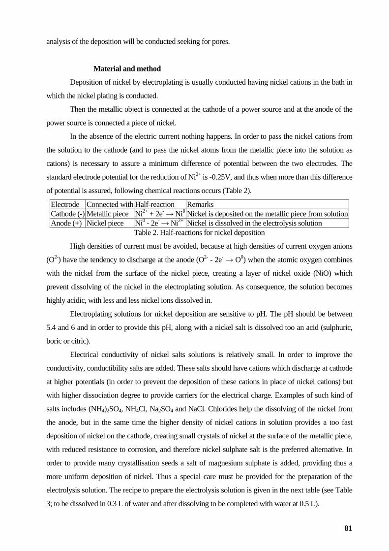
analysis of the deposition

2).

Electr

will be conducted seeking for pores.

Material and method

Deposition of nickel by electroplating is usually conducted having nickel cations in the bath in

which the nickel plating is conducted.

Then the metallic object is connected at the cathode of a power source and at the anode of the

power source is connected a piece of nickel.

In the absence of the electric current nothing happens. In order to pass the nickel cations from

the solution to the cathode (and to pass the nickel atoms from the metallic piece into the solution as

cations) is necessary to assure a minimum difference of potential between the two electrodes. The

standard electrode potential for the reduction of Ni2+ is -0.25V, and thus when more than this difference

of potential is assured, following chemical reactions occurs (Table

ode Connected with Half-reaction Remarks Cathode (-) Metallic piece Ni2+ + 2e- → Ni0 Nickel is deposited on the metallic piece from solutionAnode (+) Nickel piece Ni0 - 2e- → Ni2+ Nickel is dissolved in the electrolysis solution

Table 2. Half-reactions for nickel deposition

High densities of current must be avoided, because at high densities of current oxygen anions

(O2-) have the tendency to discharge at the anode (O2- - 2e- → O0) when the atomic oxygen combines

with the nickel from the surface of the nickel piece, creating a layer of nickel oxide (NiO) which

prevent dissolving of the nickel in the electroplating solution. As consequence, the solution becomes

highly acidic, with less and less nickel ions dissolved in.

Electroplating solutions for nickel deposition are sensitive to pH. The pH should be between

5.4 and 6 and in order to provide this pH, along with a nickel salt is dissolved too an acid (sulphuric,

boric or citric).

Electrical conductivity of nickel salts solutions is relatively small. In order to improve the

ctrical charge. Examples of such kind of

salts includes (NH , NH4Cl, N SO4

the anode, but in vides a too fast

deposition of nickel on the catho he surface of the metallic piece,

ith reduced resis corrosion, and therefore nickel sulphate salt is the preferred alternative. In

3; to be dissolved in 0.3 L of water and after dissolving to be completed with water at 0.5 L).

conductivity, conductibility salts are added. These salts should have cations which discharge at cathode

at higher potentials (in order to prevent the deposition of these cations in place of nickel cations) but

with higher dissociation degree to provide carriers for the ele

4)2SO4 a2 and NaCl. Chlorides help the dissolving of the nickel from

the same time the higher density of nickel cations in solution pro

de, creating small crystals of nickel at t

w tance to

order to provide many crystallisation seeds a salt of magnesium sulphate is added, providing thus a

more uniform deposition of nickel. Thus a special care must be provided for the preparation of the

electrolysis solution. The recipe to prepare the electrolysis solution is given in the next table (see Table

81

Substance Quantity Role NiSO4·7H2O 68g Source of Ni2+

NH Cl 8g For conduction 4MgSO4·7H2O 24g Crystallisation seedling

H3BO3 2g Buffering the pH Table 3. Recipe for preparing the electrolysis solution for nickel deposition

The quality of the nickel deposition depends on the density of current. At too small current

densities the deposition is slow, the nickel crystals will grow higher and the layer deposited will be soft

d ma

ull cell [247].

e co ing an electrolytic bath connected to a power

s t

an t. At too high current densities, the nickel will be deposited as dust, the bonds between atoms

being irregularly created, and the layer have then a black colour. The optimal density of current

depends on the composition and on the size of the nickel deposition bath. For the bath to be used in the

laboratory experiment the optimal current density is DC = 0.5 A/dm2. The determination of the optimal

current density involves a series of preliminary experiments with the H

The xperiment of nickel plating is nducted us

ource (U) being interconnec ed using a variable resistor (R) and an ampere-meter (A).

Figure 1. Instrumentation for nickel plating

Working procedure

Experiment for efficiency of nickel deposition

The succession of the steps is as follows (data to be filled in Table 4):

÷ Take the (biggest) sample, polish (with abrasive paper) and degreases it (with limewater, Ca(OH)2)

if is necessary;

÷ Measure the surface of the sample (by using the ruler) and record the value (S); piece have two

sides, so please take it both into account;

÷ Calculate the ideal current intensity (Ithr) by using the ideal density of current (DC = 0.5 A/dm2);

÷ Weight the sample using the analytical balance and record the value (m1);

A

U + -

R

82

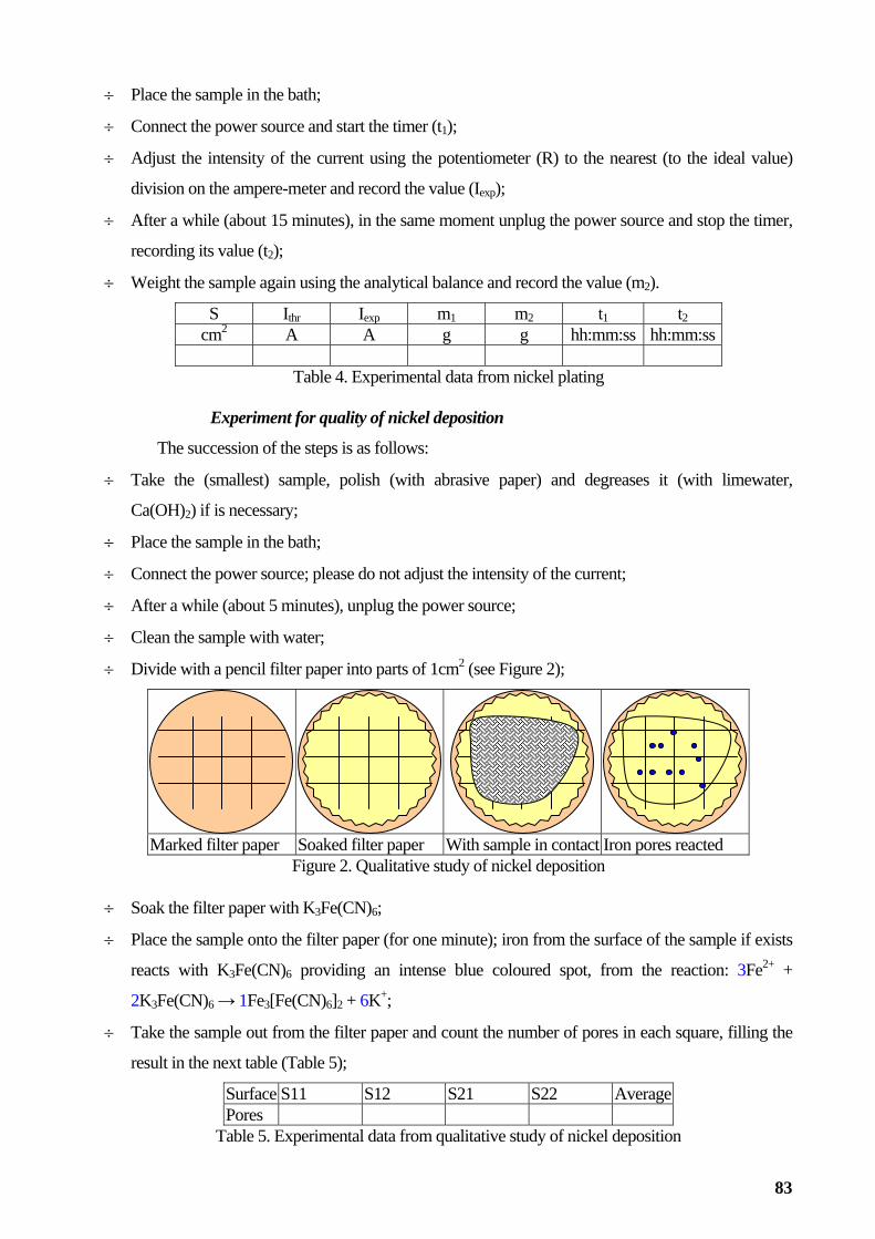
÷ Place the sample in the ba

÷ Connect the power sour ti t1);

÷ Adjust the intensity of ng p nearest (to the ideal value)

division o

After a while (about 15 minutes), in the same moment unplug the power source and stop the timer,

reco

th;

ce a t thend s art m (er

the current usi the otentiometer (R) to the

n the ampere-meter and record the value (Iexp);

÷

rding its value (t2);

÷ Weight the sample again using the analytical balance and record the value (m2).

S Ithr Iexp m1 m2 t1 t2 cm2 A A g g hh:mm:ss hh:mm:ss

Table 4. Experimental data from nickel plating

Experiment for quality of nickel deposition

The succession of the steps is as follows:

÷ Take the (smallest) sample, polish (with abrasive paper) and degreases it (with limewater,

Ca(OH)2) if is necessary;

÷ Place the sample in the bath;

÷ Connect the power source; please do not adjust the intensity of the current;

÷ After a while (about 5 minutes), unplug the power source;

÷ Clean the sample with water;

÷ Divide with a pencil filter paper into parts of 1cm2 (see Figure 2);

Marked filter paper S Iron pores reacted oaked filter paper With sample in contact

Figure 2. Qualitative study of nickel deposition

Soak the f

Place the s ple if exists

reac the reaction: 3Fe2+ +

3 6 2

Take the sample out from the filter paper and count the number of pores in each square, filling the

÷ ilter paper with K Fe(CN) ; 3 6

÷ ample onto the filter paper (for one minute); iron from the surface of the sam

ts with K Fe(CN) providing an intense blue coloured spot, from3 6

2K3Fe(CN)6 → 1Fe [Fe(CN) ] + 6K+;

÷

result in the next table (Table 5);

Surface S11 S12 S21 S22 Average Pores

Table 5. Experimental data from qualitative study of nickel deposition

83

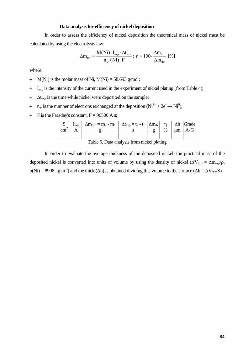
Data analysis for efficiency of nickel deposition

position the theoretical mass of nickel must be In order to assess the efficiency of nickel de

calculated by using the electrolysis law:

F)Ni(nethr ⋅

tI)Ni(Mm expexp Δ⋅⋅

=Δ ; − thrmΔ

expm00

Δ1 ⋅ [%]

÷ Iexp is the in sity of t urrent u n the experiment of nickel plating (from Table 4);

÷ Δtexp is the time wh e el were deposited on the sample

÷ ne- is the number of elec 0);

F is he Far

texp = t2 - t1 Δmthr η Δh Grade

=η

where:

÷ M(Ni) is the molar mass of Ni, M(Ni) = 58.693 g/mol;

ten he c sed i

il nick ;

trons exchanged at the deposition (Ni2+ + 2e- → Ni

÷ t aday's constant, F = 96500 A·s;

S Iexp Δmexp = m2 - m1 Δcm2 A g s g % μm A-G

Table 6. Data analysis from nickel plating

average thickness of the deposited nickel, the practical mass of the

ckel (ΔVexp = Δmexp/ρ,

s volume to the surface (Δh = ΔVexp/S).

In order to evaluate the

deposited nickel is converted into units of volume by using the density of ni

ρ(Ni) = 8908 kg·m-3) and the thick (Δh) is obtained dividing thi

84

Producing electricity from electrochemical cells

An electrochemical cell is a device capable of her generating e al energy from chemical

reactions or facilitating chemical reactions through the introduction of electrical energy.

An electrochemical cell can be created by placing electrodes into an electrolyte where a

t (see Table 1). Electrochemical cells which

ochemical

mical reaction which would not occur

ions take place in electrochemical cells. Spontaneous

reactions occur in alv ( th c nt y r it, while

nonspontaneous ctio olytic cells and then the electric cur s sary to it. Both

types of cells contain two elec ation and reduction reactions

ccur. Naming convention is that the oxidation occurs at the electrode named anode and reduction

Cell Reaction Anode Cathode Electrical current

Introduction

eit lectric

chemical reaction either uses or generates an electric curren

generate an electric current are called voltaic cells or galvanic cells while in the other electr

cells an externally supplied electric current is used to drive a che

spontaneously, and such cells are called electrolytic cells.

Redox (reduction and oxidation) react

g anic voltaic) cells and en the electri curre ma be p oduced from

rea ns occur in electr rent i neces

trodes (anode and cathode) where the oxid

o

occurs at the electrode named cathode. Thus, in both galvanic and electrolytic cells, oxidation takes

place at the anode, reduction takes place at the cathode, and electrons flow from the anode to the

cathode (see Table 1).

Galvanic Spontaneous Negative Positive Is produced during the chemical reaction Electrolytic Nonspontaneous Positive Negative Is consumed to produce the chemical reaction

Table 1. Naming conventions for electrochemical cells

Common batteries consist of one or more galvanic cells. A galvanic cell can be created using as

electrodes any two different metals since metals differ in their tendency to lose electrons. Zinc more

readily loses electrons than copper, so placing zinc and copper metal in solutions of their salts can cause

electrons to flow through an external wire which leads from the zinc to the copper. As a zinc atom

provides the electrons, it becomes a positive ion and goes into aqueous solution, decreasing the mass of

the zinc electrode. On the copper side, the two electrons received allow it to convert a copper ion from

solution into an uncharged copper atom which deposits on the copper electrode, increasing its mass.

Half-reaction Type Electrode Charge Potential

Zn Cu

ZnSO4 CuSO4Zn(s) → Zn2+(aq) + 2e- oxidation anode negative +0.763

Cu2+(aq) + 2e- → Cu(s) reduction cathode positive +0.337

Table 2. Typical example of a galvanic cell (Daniell)

85

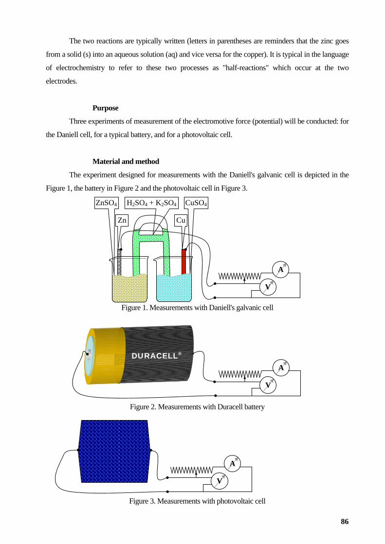
The two reac rs that the zinc goes

om a solid (s) into an aqueous solution (aq) and vice versa for the copper). It is typical in the language

e two processes as "half-reactions" which occur at the two

Figure 3. Measurements with photovoltaic cell

tions are typically written (letters in parentheses are reminde

fr

of electrochemistry to refer to thes

electrodes.

Purpose

Three experiments of measurement of the electromotive force (potential) will be conducted: for

the Daniell cell, for a typical battery, and for a photovoltaic cell.

Material and method

The experiment designed for measurements with the Daniell's galvanic cell is depicted in the

Figure 1, the battery in Figure 2 and the photovoltaic cell in Figure 3.

Figure 1. Measurements with Daniell's galvanic cell

Figure 2. Measurements with Duracell battery

A

V

CuSO4ZnSO4

Zn Cu

H2SO4 + K2SO4

A

V

DURACELL® A

V

86

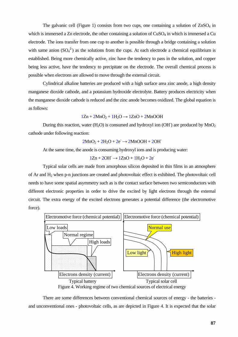
The galvanic cell (Figure 1) consists from two cups, one containing a solution of ZnSO4 in

which is immersed a Zn electrode, the other containing a solution of CuSO4 in which is immersed a Cu

electrode. The ions transfer from one cup to another is possible through a bridge containing a solution

with same anion (SO42-) as the solutions from the cups. At each electrode a chemical equilibrium is

stablished. Being more chemically active, zinc have the tendency to pass in the solution, and copper

e tendency to precipitate on the electrode. The overall chemical process is

urface area zinc anode, a high density

anganese dioxide cathode, and a potassium hydroxide electrolyte. Battery produces electricity when

the zinc anode becomes oxidized. The global equation is

follo

OH

During this reaction, water (H2O) is co and hydroxyl ion (OH-) are produced by MnO2

cathode under following reaction:

2MnO2 + 2H2O + 2e- → 2MnOOH + 2OH-

At the same time, the anode is consuming hydroxyl ions and is producing water:

1Zn + 2OH- → 1ZnO + 1H2O + 2e-

Typical solar cells are made from amorphous silicon deposited in thin films in an atmosphere

of Ar and H2 when p-n junctions are created and photovoltaic effect is exhibited. The photovoltaic cell

needs to have some spatial asymmetry such as is the contact surface between two sem

different electronic prop ns through the external

ircuit. The extra energy of the excited electrons generates a potential difference (the electromotive

force).

e

being less active, have th

possible when electrons are allowed to move through the external circuit.

Cylindrical alkaline batteries are produced with a high s

m

the manganese dioxide cathode is reduced and

as ws:

1Zn + 2MnO2 + 1H2O → 1ZnO + 2MnO

nsumed

iconductors with

erties in order to drive the excited by light electro

c

Electromotive force (chemical potential)

Electrons density (current)

Low loads Normal regime

High loads

Electromotive force (chemical potential)

Electrons density (current)

Low light High light

Normal use

Typical battery Typical solar cell Figure 4. Working regime of two chemical sources of electrical energy

There are some differences between conventional chemical sources of energy - the batteries -

and unconventional ones - photovoltaic cells, as are depicted in Figure 4. It is expected that the solar

87

ce rovide a constant current for any illumination level while the voltage to be determined by the

resistance of the load. The main difference consists in the internal resistance: the photovoltaic cell have

much higher (than the battery) internal resistance, and thus is expected that the photovoltaic cell to act

as a current source, while the battery to act as a voltage source.

Working procedure

For each experiment (out of three) the succession of the steps is a

ll to p

s follows (data to be filled in

measurement;

÷ Take one measurement o

Ad

÷ Take the second measure ;

Con oth apparatus

indicate a sensitive change of

Tak

Table 3):

÷ Connect the external load (variable resistance, ampere-meter and voltmeter) to the cell;

÷ Adjust the load (using the variable resistance) to have on both apparatus the values inside of the

scale of

f the voltage (U) and of the intensity (I);

÷ just the load (using the variable resistance) while both apparatus indicate a sensitive change of

the measured values;

ment of the voltage (U) and of the intensity (I)

÷ tinue (in same direction) to adjust the load (using the variable resistance) while b

the measured values;

÷ e the third measurement of the voltage (U) and of the intensity (I);

÷ For the photovoltaic cell is preferable to take two more measurements.

Daniell's cell Battery Solar cell No Voltage (U) Intensity (I) 1 V1 = I1 = 2 V2 = I2 =

No Voltage (U) Intensity (I)1 V1 = I1 = 2 V2 = I2 =

No Voltage (U) Intensity (I)1 V1 = I1 = 2 V2 = I2 =

3 V3 = I3 = 3 V3 = I3 = 3 V3 = I3 = 4 V4 = I4 = 5 V3 = I5 =

Table 3. Experimental data from chemical cells measurements

Data analysis for electromotive force of the chemical cells

It's expected to obtain a linear dependence of the voltage relative to intensity for the Daniell's

cell and the battery and it's expected to be a nonlinear dependence for the solar cell.

Let's consider the electrical circuit associated with the experiment (see Figure 5).

Figure 5. Electrical circuit used in the measurements

Applying the continuous current laws for the circuits (Kirchhoff's laws) and for the consumers

R3

U R1 R2 E; r I

88

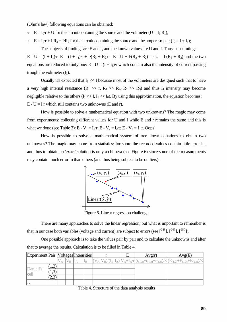
(Ohm's law) following equations can be obtained:

÷ E = I0·r + U for the circuit containing the source and the voltmeter (U = I1·R1);

÷ E = I0·r + I·R3 + I·R2 for the circuit containing the source and the ampere-meter (I0 = I + I1);

The subjects of findings are E and r, and the known values are U and I. Thus, substituting:

- U = (I + I )·r, E = (I + I )·r + I·(R + R ) = E - U + I·(R3 + R2) → U = I·(R3 + R2) and the two

quatio + I )·r which contain also the intensity of current passing

1

s expected that I << I because most of the voltmeters are designed such that to have

ay become

ns two unknowns (E and r).

nknowns? The magic may come

1 = I1·r; E - V2 = I2·r; E - V3 = I3·r. Oops!

equations to obtain two

(see Figure 6) since some of the measurements

).

important to remember is

nknowns and after

Voltages Intensities r E Avg(r) Avg(E)

E 1 1 3 2

e ns are reduced to only one: E - U = (I 1

trough the voltmeter (I ).

Usually it' 1

a very high internal resistance (R1 >> r, R1 >> R2, R1 >> R3) and thus I1 intensity m

negligible relative to the others (I1 << I, I1 << I0). By using this approximation, the equation becomes:

E - U = I·r which still contai

How is possible to solve a mathematical equation with two u

from experiments: collecting different values for U and I while E and r remains the same and this is

what we done (see Table 3): E - V

How is possible to solve a mathematical system of tree linear

unknowns? The magic may come from statistics: for shore the recorded values contain little error in,

and thus to obtain an 'exact' solution is only a chimera

may contain much error in than others (and thus being subject to be outliers

Figure 6. Linear regression challenge

There are many approaches to solve the linear regression, but what is

that in our case both variables (voltage and current) are subject to errors (see [248], [249], [250]).

One possible approach is to take the values pair by pair and to calculate the u

that to average the results. Calculation is to be filled in Table 4.

Experiment Pair VA VB IA IB (VA-VB)/(IB-IA) VA+IA·r (r(1,2)+r(1,3)+r(2,3))/3 (E(1,2)+E(1,3)+E(2,3))/3

(1,2) (1,3) Daniell's

cell (2,3)

… Table 4. Structure of the data analysis results

(x1,y1) (xi,yi) (xn,yn)

Lin )ear( y,x

89

Further reading

Other papers dealing with regression between measured variables which may be consulted are:

the

[251], [252], [253], [254], [255], [256], [257], [258], [259], [260] and [261].

When the available software does not provide the desired procedure of calculation,

alternative is to build up the calculation procedure by using calculation libraries of generic software

(see [262], [263], [264]).

90

Safety precautions in the laboratory

try.

Purpose

Recognition of laboratory safety and health problems has crystallized since the passage of the

Occupational Safety and Health Act of 1970 [265]. Safety and health considerations are as important as

any other materials taught in curricula. Occupational studies indicate that the injury rate is highest

during the initial period of engagement and decreases with experience. In a laboratory where students

experience new activities, the likelihood of incidents, injury, and damage is high. Therefore, it is

essential that the students are taught what can go wrong, how to prevent such events from occurring,

and what to do in case of an emergency.

General safety measures

When experiments require and the working procedure indicates, approved safety eye glasses or

goggles must be worn at all times. There is usually not an increased risk of chemical exposure if you

choose to wear contact lenses. The most common exceptions to this are isopropyl alcohol vapours,

ethyl alcohol vapours, methylene chloride, and ethylene oxide.

If anything gets in your eye, the eyelids should be held open while flushing the eye with water from the

eyewash for 15 minutes. The first 10 seconds are crucial. Immediately go to the nearest eye wash

station (at sinks or in the front safety station) and begin flushing the eye. Someone should notify the

instructor. Chemical burn hazards, especially hazardous to the eye are concentrated acids and bases,

bromine, aluminium chloride and ammonium sulphide.

If there is an accident or injury in the lab, take the appropriate safety measures immediately and

then notify the instructor. If there is a large chemical spill on the clothing, the safety shower should be

used immediately. Clothing should be removed promptly in the case of a large chemical spill. Wash

any chemical off on the skin with water. If your clothing catches on fire, lie down and roll. Someone

will bring the fire blanket to you. Please do not run to the blanket or safety shower. Simply smothering

it with a sufficiently large watch glass or inverted beaker can put out a small, contained fire. In the case

of a multi-neck flask, loosely insert rubber stoppers or corks. Never use a towel - it may overturn the

container and spread the fire as well as catch fire itself.

To extinguish an open fire in the laboratory, discharge the small fire extinguishers in the lab.

Introduction

Before starting activity in the laboratory it is necessary to know safe practices that must be

followed all times. It is expected to read these rules thoroughly and to pass an exam before beginning

the lab work in chemis

91

Discharge at the base or so side to the other to avoid

ashback, while calling for assistance and for the sounding of local alarms, if necessary. If the fire is

to spread, have the fire department called while using the larger

f chemicals

Some solvents are flammable and require precautions concerning there use. Three common

ents are diethyl ether, petroleum ether, and carbon disulfide. All flames and

azards, the following chemicals should be used in the hood

nly: ammonium hydroxide, concentrated acids (such as nitric, acetic, sulphuric, and hydrochloric

nhydride, and aniline.

ell as oxalates of heavy metals are

mpounds containing one of these elements or

ns: sil

urce of the flames, slowly moving from one

fl

not brought under control and begins

extinguisher in the hall. Evacuate everyone from the lab except those involved in extinguishing the fire.

Handling o

extremely flammable solv

spark sources (motors and heaters) must be turned off in the area that is used for the solvent. A hood

must be used for transferring or working with any amount of flammable solvent.

Five common less dangerous, but still highly flammable solvents are acetone, benzene,

cyclohexane, ethanol, and methanol. All flame and spark sources in their immediate area should be

turned off and a hood should be used for everything except washing glassware. The vapours of all of

the above solvents are harmful and should not be inhaled.

In order to prevent respiratory h

o

acids), ammonium sulphide, acetaldehyde, acetic a

Although will not be attempted to work with explosive hazards in the lab, their existence and

potential danger should be known. Organic compounds may react violently with the following

substances: ammonium nitrate, potassium chlorate, dichromate ion, permanganate ion, sulphur,

perchlorate ion. Solid compounds of silver or mercury as w

explosive. Iodine combined with ammonia or aluminium is an explosive reaction.

Bioaccumulants are cumulative poisons, substances that can accumulate in the body and cause

health problems. Avoid breathing the dust of these substances. Never dispose of these substances or

solutions containing these substances in the drain. Special waste containers will be provided.

Cumulative poisons include, but are not limited to, co

io ver, lead, antimony, arsenic, beryllium, mercury, cadmium, chromate, dichromate, fluoride.

In the case of liquid mercury, the most likely source is a broken thermometer. It is important

that you notify the instructor of any broken thermometers so that special equipment can be used to

clean up the spill.

A hood is used to draw toxic or flammable vapours from the laboratory. If are doubts about the

efficiency of the hood, the instructor should be asked (to test the airflow). The hood should be used in

the case of any doubts about the reaction or toxicity of the compound in use or being produced.

92

Common sense safety rules

Please follow the next rules:

÷ Never taste chemicals;

÷ Do not breathe vapours directly and waft the odour toward your nose instead;

÷ Treat a test tube with contents that you are heating like a loaded gun and thus never point it in

the side and never fill more than half full;

Wh

Do

When using glass tubing, all ends

than 5 cm) the rubber

stopper, and insert using

to do so;

Do

sterous

conduct in the laboratory and never run in the laboratory;

÷ The use of personal audio or video equipment is prohibited in the laboratory;

anyone’s direction, heat gently along

÷ en pouring liquid chemicals, use a stirring rod to direct the flow;

÷ Flush sink drains with water after disposing of chemicals there;

÷ Never return unused solutions of chemicals to the container reagent bottle;

÷ Add one reagent to another cautiously and slowly;

÷ not add any solid to a liquid over another near to the boiling point of one of them or when the

difference of the temperatures is high;

÷ Please avoid to use mouth suction to fill pipettes;

÷ Do not use glassware with broken or chipped edges

÷ should be fire polished; to insert glass tubing or rods or

thermometers into rubber stoppers, be sure you have the proper size, lubricate the glass with water

or glycerine, wrap a towel around the glass, hold the glass near to (less

pressure on the stopper;

÷ Discard broken glassware in the special glassware collection container and do not discard paper

waste with chemical waste;

÷ Do not store reagents or chemicals in lockers unless you are specifically directed by the instructor

÷ Do not use ice from the laboratory ice machine for beverages;

÷ Long hair, beards, and neckties can be dangerous in the lab because they can catch fire, get into

chemicals, or get caught in apparatus, and therefore secure hair and beard out of the way and

remove any neckties or scarves;

÷ not wear flared or loose hanging sleeves or scarves; Sandals are not acceptable shoes for lab

work and cotton clothing (e.g.; jeans) is safer than polyester.

General behaviour

When conducting laboratory works, please take into consideration that:

÷ Horseplay or other acts of carelessness are prohibited; do not engage in practical jokes or boi

93

÷ Keeping your work space neat and clean is a matter of survival;

Never work alone in the laboratory;

t items should be returned to their proper place after use;

-term in hoods;

be certain that an

sult in severe

emicals are dangerous,

event, unauthorized removal is illegal;

ry;

ical condition that might present a problem (for

nancy);

ver attempt to catch a falling object;

;

unsen burners unattended;

ted area near to the laboratory door,

work space at the end of the laboratory session;

Please keep your hands away from your face, eyes, mouth, and body while using chemicals.

ld never be brought into the laboratory or chemical storage area.

after removing gloves,

÷

÷ Reagents and equipmen

÷ Recipients containing reagents, solutions, glassware shall not be stored for long

÷ All containers must be labelled identifying its contents, otherwise should not be used;

÷ Unauthorized experiments are not permissible because students can not

experiment is safe to perform; please be aware that infractions of this rule will re

academic penalties;

÷ Chemicals may not be removed from the laboratory because most ch

particularly under non-laboratory conditions; in any

÷ Because of the risk of getting toxic chemicals into your mouth, you are not permitted to smoke,

chew, eat, or drink while in the laborato

÷ Please inform the instructor if you have any phys

example, allergies, epilepsy, breathing disorders, preg

÷ Do not perform any experiment while under the influence of drugs or alcohol; besides the obvious

danger of this, the vapours of some chemicals are toxic when combined with alcohol in the blood

(especially carbon tetrachloride);

÷ Never leave experiments while in progress and ne

÷ Be careful when handling hot glassware and apparatus in the laboratory, because hot glassware

looks just like cold glassware

÷ Make sure no flammable solvents are in the surrounding area when lighting a flame and do not

leave lit B

÷ Coats, bags, and other personal items must be stored in designa

not on the bench tops or in the aisle ways and keep the working area neat and free of any

unnecessary objects;

÷ Thoroughly clean your laboratory

Hygiene practices

Food and drink, open or closed, shou

Do not apply cosmetics while in the laboratory or storage area. Wash the hands

and before leaving the laboratory.

94

Legal provisions in labour safety

National regulations on the subject are (in force on March 20, 2015 [266]):

Official Gazette,

part I, no. 47

safety, published in the Romanian Official Gazette, part I, no. 882 from

ation of

ce 96/2003 on maternity protection at workplaces updated and

from March

uct safety, republished in the Romanian Official Gazette, part I, no.

ility for damages caused by defective products, republished in

riods of extreme temperatures to protect the employees', published in the

Law 202/2002 on equal opportunities between women and men, republished in the Romanian

arch 1, 2007;

Law

upplementing the Labour Protection Law 90/1996, published in the

Romanian Official Gazette, part I, no. 522 from October 24, 2000;

÷ Law 155/2000 for approving the Government Emergency Ordinance 16/2000 regarding the

÷ Law 319/2006 - Law on safety and health at work, published in the Romanian

part I, no. 646 from July 26, 2006;

÷ Law 90/1996 - Labour Protection Law, republished in the Romanian Official Gazette,

from January 29, 2001;

÷ Government Decision 1425/2006 approving the Methodological Norms for the application of Law

319/2006 for labour

October 30, 2006;

÷ Government Decision 955/2010 amending and supplementing the Norms for the applic

Law 319/2006 for labour safety, published in the Romanian Official Gazette, part I, no. 661 from

September 27, 2010;

÷ Law 53/2003 - Labour Code, updated and republished in the Romanian Official Gazette, part I, no.

345 from May 18, 2011;

÷ Law 108/1999 for the establishment and organization of the labour inspection, republished in the

Romanian Official Gazette, part I, no. 740 from October 10, 2002;

÷ Government Emergency Ordinan

approved by Law 25/2004, published in the Romanian Official Gazette, part I, no. 214

11, 2004;

÷ Law 245/2004 on general prod

899 from December 28, 2007;

÷ Law 240/2004 on producer responsib

the Romanian Official Gazette, part I, no. 313 from April 22, 2008;

÷ Law 436/2001 for approving the Government Emergency Ordinance 99/2000 on measures that can

be applied during pe

Romanian Official Gazette, part I, no. 404 from July 20, 2001;

÷

Official Gazette, part I, no. 150 from M

÷ 320/2001 for approving the Government Emergency Ordinance 137/1999 amending and

supplementing Law 108/1999 on the establishment and organization of the labour inspection,

published in the Romanian Official Gazette, part I, no. 344 from July 28, 2001;

÷ Law 177/2000 amending and s

95

ratification of conventions adopted by the International Labour Organization, published in the

Rom

o. 355 from July 27, 1999;

us, or heavy conditions, published in the Romanian Official Gazette, part

September 12, 2014;

ngerous substances and preparations, published in the Romanian Official

zette, part I, no. 899 from October 7, 2005;

s, published in the Romanian

anian Official Gazette, part I, no. 360 from August 2, 2000;

÷ Law 130/1999 on certain measures of protection for persons in employment, published in the

Romanian Official Gazette, part I, n

÷ Law 31/1991 on the establishment of working time under 8 hours/day for employees working in

special harmful, dangero

I, no. 654 from December 31, 1999;

÷ Law 126/1995 on the regime of explosive materials republished in the Romanian Official Gazette,

part I, no. 177 from

÷ Law 211/2011 about the regime of the wastes, republished in the Romanian Official Gazette, part I,

no. 220 from March 28, 2014;

÷ Law 360/2003 on da

Gazette, part I, no. 635 from September 5, 2003, and modified by the law 263/2005, published in

the Romanian Official Ga

÷ Law 451/2001 for approving the Government Emergency Ordinance 200/2000 on classification,

labelling and packaging of substances and chemical preparation

Official Gazette, part I, no. 416 from July 26, 2001.

96

Student's obligations for conducting experiments in the laboratory

Laboratory of chemistry takes place during the first semester having 7 meetings of conducting

laboratory activities. Each student will have a laboratory notebook for recording experimental

phy (second page);

/or were made (following pages).

or conducting of the each practical activity.

ry after conducting of each

first and second week of the semester). Safety

measures in the laboratory are assumed. It is conducted a demonstrative experiment: Study gaseous

diffusion and molecular velocities. Each student will record (individually) the observed values and

will perform all the calculations (same rule applies for the rest of the lab activities).

2. At this point the notebooks must be up to date (during the third and fourth week of the semester). It

is conducted a frontal experiment: Obtaining of the oxygen: study of the gases laws. At this

moment students will be divided into working groups (of 2 to 5 students) for the next series of

activities which will be in a cycle (rotation; 3 → 4; 4 → 5; 5 → 6; 6 → 7; 7 → 3).

For the following activities these are planned and conducted in the assigned working group:

3. Activity to be conducted: Qualitative analysis of metals and alloys. In this (third) meeting exercises

of writing chemical formulas will be conducted too.

4. Activity to be conducted: Study of chemical reactions. In this (fourth) meeting tests of writing

chemical formulas will be given.

5. Activity to be conducted: Water analysis. In this (fifth) meeting tests of writing chemical formulas

will be given.

6. Activity to be conducted: Volumetric and gravimetric methods in study of corrosion. In this

(penultimate) meeting, quizzes tests from laboratory activities will be given.

7. Activity to be conducted: Nickel corrosion protective electroplating. In this (ultimate) meeting,

quizzes tests from laboratory activities will be given. Laboratory notebooks will be checked.

observations, processing and interpretation of results; laboratory notebook has the following structure:

÷ Name, surname, discipline (first page);

÷ List of laboratory works and bibliogra

÷ Instrumentation Laboratory - drawings and chemical formulas (pages 3 to 5);

÷ Successive series of works which will and

Tables of experimental observations, formulas, and tables processing results are compulsory to

be in the notebook before the meet f

Each student will prepare (you know) the working procedure(s) of the activity planned to be

conducted in the laboratory.

Data processing and interpretation of the results are mandato

experiment.

Practical activities are carried out as follows:

1. Presentation of the chemistry laboratory (during the

97

L dule. All

absences will be recovered. An absence (1/7) is Recoveries extra charge

rom 2

ratory activities).

entary activities in the laboratory on a

approval

Conducting the m

mentary in any of the

meetings from the second one to the last one);

mination date (planned date for the exam of Chemistry) is required

or further details, please visit http://l.academicdirect.org

aboratory activities are all mandatory and should be conducted according to the sche

recovered without charge.

(f /7 to 7/7) must be planned in advance with the supervisor.

Laboratory activity is recorded with admitted/rejected. In order to pass the chemistry

laboratory, each student must attend and conduct all 7 laboratory activities and to pass both tests (of

chemical formulas and of quizzes from labo

Possible bonuses may be archived doing supplem

voluntary basis. These require knowing of the working procedure and are possible only after

of the supervisor:

÷ easurements with the Analytical balance (for all groups);

÷ Producing electricity from electrochemical cells (to be conducted supple

At the moment of the exa

that each student to have given at least once the test from theory on the computer (in the presence of a

supervisor). F and consult the following works: 270 271 272 273 64[ ], [ ], [ ], [ ], [ ], [ ], [ ] and [ ]. 267 268 269

98

99

References

1 L JÄNTSCHI, Romeo CHIRA, 2000. Book of practical works for chemistry and biochemistry of pollutants (in

anian). Cluj-Napoca: UTPres, 113 p. 2 Horea I. NAŞCU, Liana T. MARTA, Elena M. PICĂ, Violeta POPESCU, Mihaela L. UNGUREŞAN, Lorentz

JÄNTSCHI, 2002. Chemistry - practical works guide (in Romanian). Cluj-Napoca: UTPres, 159 p. 3 Lorentz JÄNTSCHI, Mihaela L. UNGUREŞAN, 2002. Physical chem

orentzRom

istry. Experiments of chemical and instrumental analysis (in Roman

orentz

58 p. 013. Presentation and processing of the experimental data (in Romanian & English). Cluj-Napoca:

s of Thought. New York:

Isaac http:

ian). Cluj-Napoca: Amici, 120 p. 4 L JÄNTSCHI, Sorana D. BOLBOACĂ, 2003. Applied chemical and instrumental analysis (in Romanian). Cluj-

Nanpoca: AcademicDirect, 60 p. 5 Lorentz JÄNTSCHI, 2013. Physical chemistry: theory, applications and problems (in Romanian). Cluj-Napoca:

AcademicDirect, 16 Lorentz JÄNTSCHI, 2

UTPres, 70 p. 7 George BOOLE, 1854. An Investigation of the Laws of Thought. (Reprinted 2003 as Law

Prometheus Books. ISBN 1-59102-089-1), p. 430. 8 Ronald A. FISHER, 1922. On the interpretation of χ2 from contingency tables, and the calculation of P. Journal of the Royal

Statistical Society 85(1): 87-94. 9 NEWTON, 1687. Philosophiæ naturalis principia mathematica. London: Juffu Societatis Regiæ, full text:

//www.ntnu.no/ub/spesialsamlingene/ebok/02a019654.html 10 Julian L. COOLIDGE, 1949. The Story of the Binomial Theorem. The American Mathematical Monthly 56(3): 147-157.

full text: http://www.jstor.org/stable/2305028 11 Jacobi BERNOULLI, 1713. Ars Conjectandi. Basel: Thurnisius. 12 Abraham De MOIVRE, 1738. Approximatio ad Summam Terminorum Binomii (a+b)n in Seriem expansi (presented

privately to some friends in 1733), p. 235-243 In: Thof E ts in lay ( nd e W. Pearson.

e Doctrine of Chance: or The Method of Calculating the Probability ven P 2 d.), London:

13 Johann C. F. GAUSS, 1823. Theoria combinations observationum erroribus minnimis obnoxiae. Pars prior, et Pars posterior. Comment. Societ. R. Sci. Gottingensis Recentiores 5: 33-90.

14 Abraham WALD, 1939. Contributions to the Theory of Statistical Estimation and Testing Hypothesis. The Annals of Mathematical Statistics 10(4): 299-326.

15 Allan AGRESTI, Brent A. COULL, 1998. Approximate is Better than "Exact" for Interval Estimation of Binomial Proportions. American Statistician 52(2): 119-126.

16 Allan AGRESTI, Yongyi MIN, 2001. On small-sample confidence intervals for parameters in discrete distributions. Biometrics 57(3): 963-971.

17 Allan AGRESTI, 2001. Exact inference for categorical data: Recent advances and continuing controversies. Statistics in Medicine 20(17-18): 2709-2722.

18 Allan AGRESTI, 2002. Dealing with discreteness: Making 'exact' confidence intervals for proportions, differences of proportions, and odds ratios more exact. Statistical Methods in Medical Research 12(1): 3-21.

19 Wolfgang K. ENGEL, 1973. Onset of synthesis of mitochondrial enzymes during mouse development. Synchronous activation of parental alleles at the gene locus for the M form of NADP dependent malate dehydrogenase. Humangenetik 20(2): 133-140.

20 David L. MEADOWS, Jerome S. SCHULTZ, 1991. A molecular model for singlet/singlet energy transfer of monovalent ligand/receptor interactions. Biotechnology and Bioengineering 37(11): 1066-1075.

21 Mark D. SZCZELKUN, 2002. Kinetic models of translocation, head-on collision, and DNA cleavage by type I restriction endonucleases. Biochemistry 41(6): 2067-2074.

22 Tijen TANYALÇIN, François J. M. EYSKENS, Eddy PHILIPS, Marc LEFEVERE, Benal BÜYÜKGEBIZ, 2002. A marked difference between two populations under mass screening of neonatal TSH and biotinidase activity. Accreditation and Quality Assurance 7(11): 498-506.

23 Enrique A. OSSET, Mercedes FERNÁNDEZ, Juan A. RAGA, Aneta KOSTADINOVA, 2005. Mediterranean Diplodus annularis (Teleostei: Sparidae) and its brain parasite: Unforeseen outcome. Parasitology International 54(3): 201-206.

24 Clarke R. CONANT, Marc R. Van GILST, Stephen E. WEITZEL, William A. REES, Peter H. von HIPPEL, 2005. A Quantitative Description of the Binding States and In Vitro Function of Antitermination Protein N of Bacteriophage? Journal of Molecular Biology 348(5): 1039-1057.

25 Matthew A. CARLTON, William D. STANSFIELD, 2005. Making babies by the flip of a coin? American Statistician 59(2): 180-182.

26 Sorana D. BOLBOACĂ, Lorentz JÄNTSCHI, Tudor DRUGAN, Andrei ACHIMAŞ-CADARIU, 2004. Creating therapy studies critical appraised topics. CatRom original software for Romanian physicians. Applied Medical Informatics 15(3-4): 26-33.

27 Sorana D. BOLBOACĂ, Lorentz JÄNTSCHI, Andrei ACHIMAŞ-CADARIU, 2004. Creating diagnostic critical appraised topics. CatRom original software for Romanian physicians. Applied Medical Informatics 14(1-2): 27-34.

100

28 Sorana D. BOLBOACĂ, Lorentz JÄNTSCHI, Andr ADARIU, 2003. Creating etiology/prognostic critical

appraised topics. CatRom original software for Romanian physicians. Applied Medical Informatics 13(3-4): 11-16. Sorana D. BOLBOACĂ, Lorentz JÄNTSCHI, 2007. Communication of results on risk factors studies: confidence

intervals. Leonardo Journal of Sciences 6(10): 179-187.

M Cluj-Napoca. Horticulture 65(1): 71-79.

34 T LBOACĂ, Lorentz JÄNTSCHI, Andrei ACHIMAŞ-CADARIU, 2003. Binomial

tices and Technologies 2(3): 45-74.

ury Press.

ath.ist.utl.pt/~apires/AP_COMPSTAT02.pdf

ei ACHIMAŞ-C

29

30 Sorana D. BOLBOACĂ, Lorentz JÄNTSCHI, Radu E. SESTRAS, 2008. Reporting results and associated statistics in quantitative genetic studies. Bulletin UASV

31 Ronald A. FISHER, 1925. Theory of statistical estimation. Proceedings of the Cambridge Philosophical Society 22: 700-725.

32 Ronald A. FISHER, 1912. On an Absolute Criterion for Fitting Frequency Curves. Messenger of Mathematics 41: 155-160.

33 Evan COOCH, Gary WHITE, 2011. Program MARK. A gentle introduction. Internet: E-book (22 Dec. 2011, 927p.). udor DRUGAN, Sorana D. BOdistribution sample confidence intervals estimation 1. Sampling and medical key parameters calculation. Leonardo Electronic Journal of Prac

35 Bernard ROSNER, 1995. Hypothesis Testing: Categorical Data (p. 345-442) In: Fundamentals of Biostatistics (4th ed.). Belmont: Duxb

36 Robert G. NEWCOMBE, 1998. Two-sided confidence intervals for the single proportion; comparison of seven methods. Statistics in Medicine 17(8): 857-872.

37 Ana M. PIRES, 200X. Confidence intervals for a binomial proportion: comparison of methods and software evaluation (web only). URL: http://www.m

982. Approximate Confidence Intervals for Probabilities

41 B

43 R inburgh: Oliver and Boyd.

ethods in Medical Research 12: 3-21.

38 Lawrence D. BROWN, Tony T. CAI, Anirban DasGUPTA, 2001. Interval estimasion for a binomial proportion. Statistical Science 16(2): 101-133.

39 Edwin B. WILSON, 1927. Probable Inference, the Law of Succession, and Statistical Inference. Journal of the American Statistical Association 22(158): 209-212.

40 J. R. ANDERSON, Leslie E. BERNSTEIN, Malcolm C. PIKE, 1of Survival and Quantiles in Life-Table Analysis. Biometrics 38(2): 407-416. arnet WOOLF, 1955. On estimating the relation between blood group and disease. Annals of Human Genetics 19: 251-253.

42 John J. GART, 1966. Alternative analyses of contingency tables. Journal of Royal Statistical Society B28: 164-179. onald A. FISHER, 1956. Statistical Methods for Scientific Inference. Ed

44 Charles J. CLOPPER, Egon S. PEARSON, 1934. The use of confidence or fiducial limits illustrated in the case of the binomial. Biometrika 26: 404-413.

45 Allan AGRESTI, 2003. Dealing with discretness: making ‘exact’ confidence intervals for proportions, differences of proportions, and odds ratios more exact. Statistical M

46 Harold JEFFREYS. Theory of Probability (3rd Ed). Clarendon Press, Oxford, 1961. http://lccn.loc.gov/62000074 olin R. BLYTH, Harold A. STILL, 47 C 1983. Binomial confidence intervals. Journal of the American Statistical Association

48 G nomial confidence intervals. The Canadian Journal of Statistics 14(2): 113-129.

51 L I, Sorana D. BOLBOACĂ, 2010. Exact Probabilities on Confidence Limits for Binomial Samples:

52 S tervals used in Medical Studies (in

53 S 005. Binomial distribution sample confidence intervals estimation for

54 L iversity analysis - Project proposal PN-II-ID-PCE-2011-3-0103,

55 R

57M Delia DICU, 2001. Desulfuration of waste gases from industrial

58 L I, Elena Maria PICĂ, 2003. Coals analysis by sample study. UNITECH'03 International Scientific

59 L model. Bulletin UASMV Cluj-Napoca. Horticulture 66(2): 684-690.

oca.

78(381): 108-116. eorge CASELLA, 1986. Refining bi

49 Sorana D. BOLBOACĂ, Lorentz JÄNTSCHI, 2008. Optimized Confidence Intervals for Binomial Distributed Samples. International Journal of Pure and Applied Mathematics 47(1): 1-8.

50 Lorentz JÄNTSCHI, Sorana D. BOLBOACĂ, 2007. How to Asses Dose-Response Study Outcome: a Statistical Approach. Recent Advances in Synthesys & Chemical Biology VI: P36. orentz JÄNTSCHApplied to the Difference between Two Proportions. TheScientificWorldJOURNAL 10(5): 865-878. orana D. BOLBOACĂ, Lorentz JÄNTSCHI, 2008. Assessment of Confidence InRomanian). Cluj-Napoca: AcademicPres & AcademicDirect, p. 234 (+p. 10 intro). orana D. BOLBOACĂ, Lorentz JÄNTSCHI, 2positive and negative likelihood ratio medical key parameters. Annual Symposium on Biomedical and Health Informatics. Special Issue: from Foundations to Applications to Policy. CD: 66-70. orentz JÄNTSCHI, 2011. Sampling distribution in biodnot funded (It was found "not eligible", see UEFISCDI.ro website). alph V. L. HARTLEY, 1928. Transmission of Information. Bell Syst Tech J 1928: 535-563.

56 Mihaela L. UNGUREŞAN, Lorentz JÄNTSCHI, 2001. Desulfuration of waste gases from industrial processes. Chemical methods. Oradea University Annals, Chemistry Fascicle VIII: 19-24. ihaela L. UNGUREŞAN, Lorentz JÄNTSCHI, processes. Electrochemical Methods. Oradea University Annals, Chemistry Fascicle VIII: 25-30. orentz JÄNTSCHConference 2003: 263-266. orentz JÄNTSCHI, 2009. Distribution fitting 1. Parameters estimation under assumption of agreement between observation and

60 Lorentz JÄNTSCHI, Sorana D. BOLBOACĂ, 2009. Distribution fitting 2. Pearson-Fisher, Kolmogorov-Smirnov, Anderson-Darling, Wilks-Shapiro, Kramer-von-Misses and Jarque-Bera statistics. Bulletin UASMV Cluj-Nap

101

61 So lletin

62 L ervation vs. observable: maximum likelihood estimations

, Monica ŞTEFU, Adriana F. SESTRAŞ, Marcel M. DUDA, Radu E. SESTRAŞ, Ştefan ŢIGAN, Ioan

nning of a genetic algorithm. Bulletin UASMV Cluj-Napoca. Agriculture 66(1): 82-88. UŢ,

65 M HI, Ioan ABRUDAN, 2009. (Distribution fitting 6.) Key

66 C rana D. BOLBOACĂ, Ioan ABRUDAN, Lorentz JÄNTSCHI, 2009. Student perception of

67 C BOACĂ, Ioan ABRUDAN, Lorentz JÄNTSCHI, 2010. The role of the academic

68 S E. SESTRAŞ, Doru C. PAMFIL, 2011.

69 L ur C. BĂLAN, 2009. (Distribution fitting 7.) Analysis of the genotypes number in different

70 S CHI, 2007. Design of experiments: useful orthogonal arrays for number of

71 L ording evolution supervised by a genetic

72 L JÄNTSCHI, Sorana D. BOLBOACĂ, 2013. Supervised evolution: research concerning the number of evolutions

ionships from natural

74 D rentz JÄNTSCHI, 2011. Neural network on photodegradation of octylphenol using

75 D ical-chemical parameters of 68(1-2):

76 S CĂ, Lorentz JÄNTSCHI, Radu E. SESTRAŞ, 2009. Statistical approaches in analysis of variance:

iseases attack on F-1 interspecific apple hybrids and

78 S du E. SESTRAŞ, 2010. Statistics and genetic

fic apple hybrids. Bulletin UASMV

80 And powdery mildew [podosphaera

011. Griffing experimental

82 M 013. Distribution of molecules by kinetic energy

83 M tein and Fermi-Dirac

84 M . BOLBOACĂ, Lorentz JÄNTSCHI, Radu E. SESTRAŞ, 2009. (Distribution fitting 8.)

Horticulture 66(2): 691-697. rana D. BOLBOACĂ, Lorentz JÄNTSCHI, 2009. Distribution fitting 3. Analysis under normality assumption. BuUASMV Cluj-Napoca. Horticulture 66(2): 698-705. orentz JÄNTSCHI, Sorana D. BOLBOACĂ, 2009. Obsaccording to the assumption of generalized Gauss and Laplace distributions. Leonardo Electronic Journal of Practices and Technologies 8(15): 81-104.

63 Lorentz JÄNTSCHI, Sorana D. BOLBOACĂ, Carmen E. STOENOIU, Mihaela IANCU, Monica M. MARTA, Elena M. PICĂABRUDAN, Mugur C. BĂLAN, 2009. Distribution fitting 4. Benford test on a sample of observed genotypes number from ru

64 Lorentz JÄNTSCHI, Carmen E. STOENOIU, Sorana D. BOLBOACĂ, Mugur C. BĂLAN, Liviu C. BOLUNDVioleta POPESCU, Horea I. NAŞCU, Ioan ABRUDAN, 2009. (Distribution fitting 5.) Knowledge assessment: distribution of answers to an online quizzed system. Bulletin UASMV Cluj-Napoca. Horticulture 66(2): 680-683. onica M. MARTA, Carmen E. STOENOIU, Lorentz JÄNTSCissues in choosing a university. Bulletin UASMV Cluj-Napoca. Horticulture 66(2): 816-822. armen E. STOENOIU, Sodegree of academic community involvement in academic life. Actual Problems of Economics 11(101): 276-283. armen E. STOENOIU, Sorana D. BOLcommunity in defining the professional route: students' perception. Actual Problems of Economics 103(1): 277-285. orana D. BOLBOACĂ, Lorentz JÄNTSCHI, Adriana F. SESTRAŞ, Radu Pearson-Fisher chi-square statistic revisited. Information 2(3): 528-545. orentz JÄNTSCHI, Mugselection and survival strategies. Bulletin UASMV Cluj-Napoca. Horticulture 66(1): 58-65. orana D. BOLBOACĂ, Lorentz JÄNTSexperiments from 4 to 16. Entropy 9(4): 198-232. orentz JÄNTSCHI, Sorana D. BOLBOACĂ, Radu E. SESTRAŞ, 2010. Recalgorithm for quantitative structure-activity relationship optimization. Applied Medical Informatics 26(2): 89-100. orentzthat occur under certain constraints. Chemical Biology & Drug Design 82(5): 603-611.

73 Sorana D. BOLBOACĂ, Daniela D. ROŞCA, Lorentz JÄNTSCHI, 2014. Structure-activity relatevolution. MATCH Communications in Mathematical and in Computer Chemistry 71(1): 149-172. ana M. POPA, Letitia OPREAN, Lonatural and artificial UV radiation. Applied Medical Informatics 29(3): 1-10. ana M. POPA, Letiţia OPREAN, Lorentz JÄNTSCHI, 2011. Factor analysis on physwastewater from Medias's treatment plant. Bulletin UASMV Cluj-Napoca. Animal sciences and Biotechnology 368-375. orana D. BOLBOAfrom random arrangements to Latin square experimental design. Leonardo Journal of Sciences 8(15): 71-82.

77 Radu E. SESTRAŞ, Catalina DAN, Doru PAMFIL, Adriana F. SESTRAŞ, Lorentz JÄNTSCHI, Sorana D. BOLBOACĂ, 2010. The variability of juvenile period, fruits size and response to dthe efficiency of selection. Notulae Botanicae Horti Agrobotanici Cluj-Napoca 38(1): 234-240. orana D. BOLBOACĂ, Lorentz JÄNTSCHI, Adriana F. SESTRAŞ, Raanalysis of quantitative traits using Griffing's experimental method IV: a practical guideline. Bulletin UASMV Cluj-Napoca. Horticulture 67(1): 56-64.

79 Catalina DAN, Radu E. SESTRAŞ, Adriana SESTRAŞ, Doru PAMFIL, Sorana D. BOLBOACĂ, Lorentz JÄNTSCHI, 2010. Heritability and genetic parameters estimated for fruits size in F1 interspeciCluj-Napoca. Horticulture 67(1): 65-71. driana F. SESTRAŞ, Doru PAMFIL, Catalina DAN, Sorana D. BOLBOACĂ, Lorentz JÄNTSCHI, Radu E. SESTRAŞ, 2011. Possibilities to improve apple scab (venturia inaequalis (cke.) wint.) aleucotricha (ell. et everh.) salm.] resistance on apple by increasing genetic diversity using potentials of wild species. Australian Journal of Crop Science 25(1): 2217-2221.

81 Sorana D. BOLBOACĂ, Lorentz JÄNTSCHI, Adriana D. BACIU, Radu E. SESTRAŞ, 2method II: step-by-step descriptive and inferential analysis of variances. JP Journal of Biostatistics 6(1): 31-52. onica P. FODOR, Sorana D. BOLBOACĂ, Lorentz JÄNTSCHI, 2revisited. Bulletin UASMV Cluj-Napoca. Horticulture 70(1): 10-18. onica G. HĂŞMĂŞANU, Sorana D. BOLBOACĂ, Lorentz JÄNTSCHI, 2014. Bose-Eins

distributions and their use in biological sciences. Bulletin UASMV Cluj-Napoca. Veterinary Medicine 71(1): 114-123. ugur C. BĂLAN, Sorana DWeather monitoring: wind analysis (May, 2009; GPS: Lat. N46°45'35"; Long. E23°34'19"). Bulletin UASMV Cluj-Napoca. Horticulture 66(1): 7-9.

85 Lorentz JÄNTSCHI, 2012. Distribution fitting 16. How many colors are actually in the field? Bulletin UASMV Cluj-Napoca. Horticulture 69(1): 184-188.

102

86 L D. BOLBOACĂ, 2011. Distributing correlation coefficients of linear structure-

87 L r C. BĂLAN, Radu E. SESTRAŞ, 2011. Distribution fitting 13.

technology 68(1-2): 323-331.

89 L istribution of seed size: a

90 R

orti

94 L . SESTRAŞ, 2011. Chlorophylls - natural solar

95 L dant capacity of red wine

-85.

letin UASMV Cluj-

99 L E. SESTRAŞ, 2010. Average trends over

100 L NTSCHI, Sorana D. BOLBOACĂ, Mircea V. DIUDEA, Radu E. SESTRAŞ, 2010. Average trends over

102 S correlation analysis on

103 Les 6(10): 169-187.

105 S HI, 2007. How good can the characteristic polynomial be for correlations?

106 S

107 S olecular descriptors family on structure activity relationships 3.

108 L hips 4.

-

110 Lno-6-quinazoline sulfonamide derivates. Leonardo Journal of Sciences 5(8): 77-88.

f polychlorinated biphenyls, Leonardo Electronic Journal of Practices and

orentz JÄNTSCHI, Soranaactivity/property models. Leonardo Journal of Sciences 10(19): 27-48. orentz JÄNTSCHI, Sorana D. BOLBOACĂ, MuguAnalysis of independent, multiplicative effect of factors. Application to the effect of essential oils extracts from plant species on bacterial species. Application to the factors of antibacterial activity of plant species. Bulletin UASMV Cluj-Napoca. Animal sciences and Bio

88 Lorentz JÄNTSCHI, Sorana D. BOLBOACĂ, Radu E. SESTRAŞ, 2011. Distribution fitting 12. Sampling distribution of compounds abundance from plant species measured by instrumentation. Application to plants metabolism classification. Bulletin UASMV Cluj-Napoca. Horticulture 68(1): 54-61. orentz JÄNTSCHI, Rodica C. SOBOLU, Sorana D. BOLBOACĂ, 2012. An analysis of the dcase study of the gymnosperms.Notulae Botanicae Horti Agrobotanici Cluj-Napoca 40(2): 46-52. adu E. SESTRAŞ, Lorentz JÄNTSCHI, Sorana D. BOLBOACĂ, 2012. Poisson parameters of antimicrobial activity: a quantitative structure-activity approach. International Journal of Molecular Sciences 13(4): 5207-5229.

91 Lorentz JÄNTSCHI, Sorana D. BOLBOACĂ, Radu E. SESTRAŞ, 2012. A simulation study for the distribution law of relative moments of evolution. Complexity 17(6): 52-63.

92 Anamaria D. HOSU, Claudia V. CIMPOIU, Vasile MICLAUŞ, Lorentz JÄNTSCHI, 2011. Antioxidant content of three different varieties of wine grapes. Biotechnology and Biotechnological Equipment 25(1): 2217-2221.

93 Anamaria D. HOSU, Claudia V. CIMPOIU, Nastasia POP, Vasile MICLAUŞ, Sorana D. BOLBOACĂ, Lorentz JÄNTSCHI, 2011. The analysis of different factors affecting the red wines antioxidant content. Notulae Botanicae HAgrobotanici Cluj-Napoca 39(1): 159-164. orentz JÄNTSCHI, Sorana D. BOLBOACĂ, Mugur C. BĂLAN, Radu Ecells. Bulletin UASVM Cluj-Napoca. Agriculture 68(1): 181-187. orentz JÄNTSCHI, Radu E. SESTRAŞ, Sorana D. BOLBOACĂ, 2013. Modeling the antioxifrom different production years and sources under censoring. Computational and Mathematical Methods in Medicine 2013: a267360 (7p).

96 Lorentz JÄNTSCHI, Sorana D. BOLBOACĂ, 2014. Rarefaction on natural compound extracts diversity among genus. Journal of Computational Science 5(3): 363-367.

97 Lorentz JÄNTSCHI, Sorana D. BOLBOACĂ, Mugur C. BĂLAN, Radu E. SESTRAŞ, 2010. Tendency of evolution supervised by genetic algorithms. Bulletin UASMV Cluj-Napoca. Horticulture 67(1): 80

98 Lorentz JÄNTSCHI, Sorana D. BOLBOACĂ, Mircea V. DIUDEA, Radu E. SESTRAŞ, 2010. Average trends over millennia of evolution supervised by genetic algorithms. 3. Analysis of phenotypes associations. BulNapoca. Agriculture 67(1): 169-174. orentz JÄNTSCHI, Sorana D. BOLBOACĂ, Mircea V. DIUDEA, Radu millennia of evolution supervised by genetic algorithms. 2. Analysis of phenotypes. Bulletin UASMV Cluj-Napoca. Agriculture 67(1): 161-168. orentz JÄmillennia of evolution supervised by genetic algorithms. 1. Analysis of genotypes. Bulletin UASMV Cluj-Napoca. Horticulture 67(1): 72-79.

101 Lorentz JÄNTSCHI, 2005. Molecular descriptors family on structure activity relationships 1. Review of the methodology. Leonardo Electronic Journal of Practices and Technologies 4(6): 76-98. orana D. BOLBOACĂ, Lorentz JÄNTSCHI, 2006. Pearson versus Spearman, Kendall's taustructure-activity relationships of biologic active compounds. Leonardo Journal of Sciences 5(9): 179-200. orentz JÄNTSCHI, Sorana D. BOLBOACĂ, 2007. The jungle of linear regression revisited. Leonardo Electronic

Journal of Practices and Technologi104 Lorentz JÄNTSCHI, Sorana D. BOLBOACĂ, 2007. Results from the use of molecular descriptors family on structure

property/activity relationships. International Journal of Molecular Sciences 8(3): 189-203. orana D. BOLBOACĂ, Lorentz JÄNTSCInternational Journal of Molecular Sciences 8(4): 335-345. orana Daniela BOLBOACĂ, Lorentz JÄNTSCHI, 2005. Molecular descriptors family on structure activity relationships 2. Insecticidal activity of neonicotinoid compounds. Leonardo Journal of Sciences 4(6): 78-85. orana D. BOLBOACĂ, Lorentz JÄNTSCHI, 2005. MAntituberculotic activity of some polyhydroxyxanthones. Leonardo Journal of Sciences 4(7): 58-64. orentz JÄNTSCHI, Sorana D. BOLBOACĂ, 2005. Molecular descriptors family on structure activity relationsMolar refraction of cyclic organophosphorus compounds. Leonardo Electronic Journal of Practices and Technologies 4(7): 55-102.

109 Lorentz JÄNTSCHI, Mihaela L. UNGUREŞAN, Sorana D. BOLBOACĂ, 2005. Complex structural information integration: inhibitor activity on carbonic anhydrase II of substituted disulfonamides. Applied Medical Informatics 17(34): 12-21. orentz JÄNTSCHI, Sorana D. BOLBOACĂ, 2006. Molecular descriptors family on structure activity relationships 5. Antimalarial activity of 2,4-diami

111 Lorentz JÄNTSCHI, Sorana D. BOLBOACĂ, 2006. Molecular descriptors family on structure activity relationships 6. Octanol-water partition coefficient o

103

112 f structure-toxicity relationship of alkyl metal

113 SXIX(2): 204-209.

ure 62: 35-40.

744.

ntegration of structure information. Computer-Aided Chemical

118 L : characterization,

119 Setari Stiintifice Universitatea Bacau Seria Biologie 12(1): 50-56.

characterization. International Journal of Molecular

121 roach. Archives of Medical Science 4(1): 7-15.

logy 11(3): a9

125 S NTSCHI, 2008. Modelling analysis of amino acids hydrophobicity. MATCH-

126 utting: relationships between acelazolamide structures and their inhibitory activity. Applied

127 L polychlorinated biphenyls. Journal of Molecular Modeling 16(2): 377-386.

: 1978-1989.

nships. Folia medica 52(3): 37-45.

(8): 1617-1639.

136 S BOACĂ, Lorentz JÄNTSCHI, Radu E. SESTRAŞ, 2011. Dependence between determination coefficient

137 L SCHI, Sorana D. BOLBOACĂ, 2010. The relationship between energy calculations and boiling points of

138 L ice

139 S

Technologies 5(8): 71-86. Sorana D. BOLBOACĂ, Lorentz JÄNTSCHI, 2006. Modeling ocompounds by integration of complex structural information. Therapeutics: Pharmacology and Clinical Toxicology X(1): 110-114. orana D. BOLBOACĂ, Claudia FILIP, Ştefan ŢIGAN, Lorentz JÄNTSCHI, 2006. Antioxidant efficacy of 3-indolyl derivates by complex information integration. Clujul Medical LX

114 Lorentz JÄNTSCHI, Sorana D. BOLBOACĂ, 2006. Modelling the inhibitory activity on carbonic anhydrase IV of substituted thiadiazole- and thiadiazoline- disulfonamides: integration of structure information. Electronic Journal of Biomedicine 2006(2): 22-33.

115 Sorana D. BOLBOACĂ, Lorentz JÄNTSCHI, 2006. Molecular descriptors family on structure-activity relationships: modeling herbicidal activity of substituted triazines class. Bulletin UASMV Cluj-Napoca. Agricult

116 Lorentz JÄNTSCHI, Sorana D. BOLBOACĂ, 2007. Modeling the octanol-water partition coefficient of substituted phenols by the use of structure information. International Journal of Quantum Chemistry 107(8): 1736-1

117 Sorana D. BOLBOACĂ, Lorentz JÄNTSCHI, 2007. Modelling the inhibitory activity on carbonic anhydrase I of some substituted thiadiazole and thiadiazoline-disulfonamides: iEngineering 24(2007): 965-970. orentz JÄNTSCHI, Sorana D. BOLBOACĂ, 2007. Antiallergic activity of substituted benzamidesestimation and prediction. Clujul Medical LXXX(1): 125-132. orana D. BOLBOACĂ, Lorentz JÄNTSCHI, 2007. Structure versus biological role of substituted thiadiazole- and thiadiazoline- disulfonamides. Studii si Cerc

120 Lorentz JÄNTSCHI, Sorana D. BOLBOACĂ, Mircea V. DIUDEA, 2007. Chromatographic retention times of polychlorinated biphenyls: from structural information to propertySciences 8(11): 1125-1157. Sorana D. BOLBOACĂ, Lorentz JÄNTSCHI, 2008. Structure activity relationships of taxoids therein molecular descriptors family app

122 Lorentz JÄNTSCHI, Sorana D. BOLBOACĂ, 2008. A structural modelling study on marine sediments toxicity. Marine Drugs 6(2): 372-388.

123 Lorentz JÄNTSCHI, Violeta POPESCU, Sorana D. BOLBOACĂ, 2008. Toxicity caused by para-substituents of phenole on tetrahymena pyriformis and structure-activity relationships. Electronic Journal of Biotechno

124 Sorana D. BOLBOACĂ, Lorentz JÄNTSCHI, 2008. A structural informatics study on collagen. Chemical Biology & Drug Design 71(2): 173-179. orana D. BOLBOACĂ, Lorentz JÄcommunications in mathematical and in computer chemistry 60(3): 1021-1032. Sorana D. BOLBOACĂ, Monica M. MARTA, Carmen E. STOENOIU, Lorentz JÄNTSCHI, 2009. Molecular descriptors family on vertex cMedical Informatics 25(3-4): 65-74. orentz JÄNTSCHI, Sorana D. BOLBOACĂ, Radu E. SESTRAŞ, 2010. Meta-heuristics on quantitative structure-

activity relationships: study on128 Lorentz JÄNTSCHI, Sorana D. BOLBOACĂ, Radu E. SESTRAŞ, 2010. A study of genetic algorithm evolution on the

lipophilicity of polychlorinated biphenyls. Chemistry & Biodiversity 7(8)129 Sorana D. BOLBOACĂ, Lorentz JÄNTSCHI, 2008. Structure-property based model for alkanes boiling points.

International Journal of Pure and Applied Mathematics 47(1): 23-30. 130 Sorana D. BOLBOACĂ, Monica M. MARTA, Lorentz JÄNTSCHI, 2010. Binding affinity of triphenyl acrylonitriles to

estrogen receptors: quantitative structure-activity relatio131 Sorana D. BOLBOACĂ, Elena M. PICĂ, Claudia V. CIMPOIU, Lorentz JÄNTSCHI, 2008. Statistical assessment of

solvent mixtures models used for separation of biological active compounds. Molecules 13132 Lorentz JÄNTSCHI, Mircea V. DIUDEA, 2009. Subgraphs of pair vertices. Journal of Mathematical Chemistry 45(2):

364-371. 133 Lorentz JÄNTSCHI, Sorana D. BOLBOACĂ, Cristina M. FURDUI, 2009. Characteristic and counting polynomials:

modelling nonane isomers properties. Molecular Simulation 35(3): 220-227. 134 Lorentz JÄNTSCHI, Sorana D. BOLBOACĂ, 2009. Counting polynomials on regular iterative structures. Applied

Medical Informatics 24(1-2): 67-95. 135 Lorentz JÄNTSCHI, Sorana D. BOLBOACĂ, 2009. Entropy due to fragmentation of dendrimers. Surveys in

Mathematics and its Applications 4: 168-176. orana D. BOLand number of regressors: a case study on retention times of mycotoxins. Studia Universitatis Babeş-Bolyai. Series Chemia LVI(1): 157-166. orentz JÄNTn-alkanes. Studia Universitatis Babeş-Bolyai. Series Chemia LV(4): 61-68. orentz JÄNTSCHI, Sorana D. BOLBOACĂ, 2007. Triazines herbicidal assessed activity. Studii si Cercetari StiintifUniversitatea Bacau Seria Biologie 12(1): 57-62. orana D. BOLBOACĂ, Lorentz JÄNTSCHI, 2008. Modelling the property of compounds from structure: statistical

104

ion. Environmental Chemistry Letters 6(3): 175-181.

141 C NOIU, Sorana D. BOLBOACĂ, Lorentz JÄNTSCHI, 2008. Model formulation & interpretation - from

142 L y trees after a vertex cut. Entropy

143 S 9(10): 1148-1166.

lecular

145 ure-activity

146 example. Biomath 2(1): a1309089 (11p).

-76.

150 E TSCHI, 1999. Simulation of diffusion equation. Acta Tehnica Napocensis. Series Applied

151 L concurrent diffusion and reaction. Annals of West

152 R . On the Mathematical Foundations of Theoretical Statistics. Philosophical Transactions of the

153 Statistical

154 H rine Benthic Diversity: A Comparative Study. The American Naturalist 102(925): 243-

155 R es. Messenger of Mathematics 41:155-

156 J157 tions in harmonic progress (in Latin). Commentarii academiae scientiarum

158 Latin). Acta

159 L ing material points (in German).

160 J yer.

2.

166 R nical theory of heat. London, Macmillan.

169 H 9. Virial Coefficients of Selected Gases. In: CRC Handbook of Chemistry and Physics (Ed.

170 W quation of state for oxygen vapour - second

171 I , Sorana D. BOLBOACĂ, Lorentz JÄNTSCHI, 2008. Analysis of soil

methods for models validat140 Lorentz JÄNTSCHI, Carmen E. STOENOIU, Sorana D. BOLBOACĂ, 2008. A formula for vertex cuts in b-trees.

International Journal of Pure and Applied Mathematics 47(1): 17-22. armen E. STOEexperiment to theory. International Journal of Pure and Applied Mathematics 47(1): 9-16. orentz JÄNTSCHI, Sorana D. BOLBOACĂ, 2008. Informational entropy of b-ar10(4): 576-588. orana D. BOLBOACĂ, Lorentz JÄNTSCHI, 2009. Comparison of QSAR performances on carboquinone derivatives. TheScientificWorldJOURNAL

144 Sorana D. BOLBOACĂ, Lorentz JÄNTSCHI, 2011. Predictivity approach for quantitative structure-property models. Application for blood-brain barrier permeation of diverse drug-like compounds. International Journal of MoSciences 12(7): 4348-4364. Sorana D. BOLBOACĂ, Lorentz JÄNTSCHI, 2013. The effect of leverage and influential on structrelationships. Combinatorial Chemistry & High Throughput Screening 16(4): 288-297.

Sorana D. BOLBOACĂ, Lorentz JÄNTSCHI, 2013. Quantitative structure-activity relationships: linear regression modelling and validation strategies by

147 Sorana D. BOLBOACĂ, Lorentz JÄNTSCHI, 2010. Diagnostic of a QSPR model: aqueous solubility of drug-like compounds. Studia Universitatis Babes-Bolyai. Series Chemia LV(4): 69

148 Sorana D. BOLBOACĂ, Lorentz JÄNTSCHI, 2014. Sensitivity, specificity, and accuracy of predictive models on phenols toxicity. Journal of Computational Science 5(3): 345-350.

149 Lorentz JÄNTSCHI, Mihaela L. UNGUREŞAN, 2001. Physical chemistry. Molecular kinetic and dynamic (in Romanian). Cluj-Napoca: Mediamira, 159 p. lena M. PICĂ, Lorentz JÄNMathematics and Mechanics 42(II): 47-54. orentz JÄNTSCHI, Elena M. PICĂ, 2003. Numerical simulation of University of Timişoara. Series Chemistry 12(3): 1107-1112 onald A. FISHER, 1922Royal Society A 222: 309-368.

Nicholas METROPOLIS, Stanislaw ULAM, 1949. The Monte Carlo Method. Journal of the AmericanAssociation 44(247):335-341. oward SANDERS. 1968. Ma

283. onald A. FISHER, 1912. On an Absolute Criterion for Fitting Frequency Curv160. oseph L. LAGRANGE, 1811. Analytical mechanics (in French). Paris: Courcier. Leonhard EULER, 1781. ObservaPetropolitanae 7: 150-161. Leonhard EULER, 1781. Memorable numbers, in harmonic progression sums, natural occurring (inacademiae scientiarum Petropolitanae II: 45-75. udwig BOLTZMANN, 1868. Studies on the balance of kinetic energy between movWiener Berichte 58: 517-560. ames STIRLING, 1730. Differential Methods (in Latin). London: Bow

161 Lorentz JÄNTSCHI, Sorana D. BOLBOACĂ, 2014. First order derivatives of thermodynamic functions under assumption of no chemical changes revisited. Journal of Computational Science 5(4): 597-60

162 Johannes D. van der WAALS, 1873. On the continuity of the gas and liquid state (In Dutch). PhD Thesis, Leiden University, The Netherlands.

163 Andrew NOBLE, Frederick A. ABEL, 1875. Researches on explosives. Fired gunpowder. Phil Trans Roy Soc Lond 165: 49-155.

164 Otto REDLICH, Joseph N. S. KWONG, 1949. On The Thermodynamics of Solutions. Chemical Reviews 44(1): 233-244.

165 Marcellin BERTHELOT, 1879. Essay on mechanical chemistry founded on thermo chemistry (In French). Paris: Dunod. udolf CLAUSIUS, 1879. The mecha

167 Alfred WOHL, 1914. Investigation of the condition equation (In German). Zeitschrift für Physikalische Chemie (Leipzig) 87: 1-39.

168 Robert C. REID, John M. PRAUSNITZ, Bruce E. POLING, 1987. The Properties of Gases and Liquids. McGraw-Hill: New York. enry V. KEHIAIAN, 200

Lide DR). 89(6): 27-35. olfgang J. WAGNER, Johannes EWERS, Robert SCHMIDT, 1984. An e

and third virial coefficients. Cryogenics 24(1): 37-43. oan SUCIU, Constantin COSMA, Mihai TODICĂheavy metal pollution and pattern in central Transylvania. International Journal of Molecular Sciences 9(4): 434-453.

105

172 L tine and applications for a set of alloys.

173 D ements database and its applications. Oradea

174 in Romanian). Cluj-Napoca:

175 L HI, Sorin HODIŞAN, Claudia CIMPOIU, Ionela CETERAŞ, 2005. Analysis of some steroids by tlc

176 C ODIŞAN, 1999. A new mathematical model for the optimization of

177 C tz JÄNTSCHI, Teodor HODIŞAN, 1998. A new method for mobile phase optimization in

178 C phase optimization method for

179 Lorentz JÄNTSCHI, 2000. High-Tc

d magnetic properties. Second International

181 M I, 2003. Modeling of statistical kinetics fast redox reactions data. Annals

182 I, 2011. Kinetic study of saccharomyces pastorianus (carlsbergensis)

183 M hemical processes modeling. International Conference on

184 L ICĂ, 2002. Numerical kinetic chemistry. International Conference on Quality Control,

185 L ia PICĂ, 2003. New approach of well known oscilating reaction models. Annals of West

186 L NTSCHI, 2003. Kinetic biochemistry. Leonardo Journal of Sciences 2(2): 1-40.

nate. Journal of Chemical Education 67 (12): 1072-1072. eans of neutral and alkaline potassium

189 H 849. The quantitative determination of sugar and starch by means of copper sulfate (in

190 E entz JÄNTSCHI, 2004. Amperometric sensors for the analysis of the

191 L NAŞCU, 2002. Numerical description of titration. International Conference on Quality

193 L Pres, 138 p.

cation/Training/titration/

orentz JÄNTSCHI, 2002. Property investigations with an automat correlation rouActa Tehnica Napocensis, series Machines Building. Materials 45(1): 296-301. elia Maria GLIGOR, Lorentz JÄNTSCHI, 2005. Periodic system of el

University Annals, Chemistry Fascicle 12: 180-194. Lorentz JÄNTSCHI, 2003. Physical chemistry. Chemical and instrumental analysis (AcademicDirect, 64 p. orentz JÄNTSCusing optimum mobile phases. Acta Universitatis Cibiniensis, Seria F Chemia 8(1): 67-76. laudia CIMPOIU, Lorentz JÄNTSCHI, Teodor Hthe mobile phase composition in HPTLC and the comparison with other models. Journal of Liquid Chromatography and Related Technologies 22(10): 1429-1441 laudia V. CIMPOIU, Lorenhigh-performance thin-layer chromatography (HPTLC). Journal of Planar Chromatography - Modern TLC 11: 191-194. armen E. STOENOIU, Sorana D. BOLBOACĂ, Lorentz JÄNTSCHI, 2006. Mobile

steroids separation. Applied Medical Informatics 18(1-2): 17-24. Liana T. MARTA, Ion G. DEAC, Victor FRUTH, Maria ZAHARESCU,superconducting materials. Comparative study: coprecipitation vs solid state phase preparation. Second International Conference on Powder Metallurgy 2: 627-632.

180 Liana T. MARTA, Ion G. DEAC, Victor FRUTH, Maria ZAHARESCU, Lorentz JÄNTSCHI, 2000. High-Tc superconducting materials. The influence of Pb addition on the tc anConference on Powder Metallurgy 2: 633-636. ihaela L. UNGUREŞAN, Lorentz JÄNTSCH

of West University of Timişoara, Series Chemistry 12(3): 285-292. Cornelia NICOARĂ, Lorentz JÄNTSCHmultiplication, Bulletin UASVM Cluj-Napoca. Animal sciences and Biotechnology 68(1-2): 362-367. ihaela L. UNGURESAN, Lorentz JÄNTSCHI, 2003. Bioc

Materials Science and Engineering BRAMAT Proceedings 2003(4): 434-441. orentz JÄNTSCHI, Elena M. PAutomation and Robotics Proceedings 2002(1): 263-268. orentz JÄNTSCHI, Elena MarUniversity of Timisoara. Series Chemistry 12(3): 1169-1176. orentz JÄ

187 Giorgio G. BOMBI, Carlo Maccà, 1990. Titrations of monoprotic acids with sodium hydroxide contaminated by sodium carbo

188 Calvin A. BUEHLER, 1922. The oxidation of lactose, glucose, and galactose by mpermanganate. PhD Thesis in Chemistry (Advisor: Prof. Dr. Lloyd W. EVANS). Columbus: The Ohio State University. ermann von FEHLING, 1

German). Annalen der Chemie und Pharmacie 72(1): 106-113. lena M. PICĂ, Mihaela L. UNGUREŞAN, Loroxygen content. Acta Tehnica Napocensis, series Machines Building. Materials 47: 91-98. orentz JÄNTSCHI, Horea I. Control, Automation and Robotics Proceedings 2002(1): 259-262.

192 Lorentz JÄNTSCHI, 2003. Metrology and monitoring of environment (in Romanian). Cluj-Napoca: Amici, 148 p. orentz JÄNTSCHI, 2002. Chemical and instrumental analysis (in Romanian). Cluj-Napoca: UT

194 Lorentz JÄNTSCHI, 2007. Acid - base titration simulator. Online software available at URL: http://l.academicdirect.org/Edu

tion, Leonardo Journal of Sciences 1(1): 53-68.

es-Bolyai, Physics XLVIII(1SI): 278-284.

ricultural Engineering Proceedings 36:

198 M BALAN, Lorentz JÄNTSCHI, Sorana D. BOLBOACĂ, Mihai DAMIAN, 2010. Thermal solar collector

199 M LAN, Lorentz JÄNTSCHI, Sorana D. BOLBOACĂ, Monica ŞTEFU, Radu E. SESTRAŞ, 2009. Weather

78.

on,

195 Lorentz JÄNTSCHI, Horea I. NAŞCU, 2002. Free software development. 3. Numerical description of soft acid with soft base titra

196 Lorentz JÄNTSCHI, Delia GLIGOR, Mihaela L. UNGUREŞAN, 2003. Acid-base titration numerical simulator. Studia Universitatis Bab

197 Mugur C. BĂLAN, Mihai DAMIAN, Lorentz JÄNTSCHI, 2008. Solar radiation monitoring system. Proceedings of the 36-th international symposium on agricultural engineering: Actual Tasks on Ag507-517.

ugur C. behaviour in Romania. Polish Journal of Environmental Studies 19(1): 231-241. ugur C. BĂ

monitoring setup and analysis of air, soil and leaf parameters. Bulletin UASVM Cluj-Napoca. Horticulture 66(2): 672-679.

200 Mugur C. BĂLAN, Mihai DAMIAN, Lorentz JÄNTSCHI, 2008. Preliminary results on design and implementation of a solar radiation monitoring system. Sensors 8(2): 963-9

201 Lorentz JÄNTSCHI, 2011. Inference in meteorological data taken from January 8, 2011 at three different locations. MACRo 2011 Proceedings of the 3rd International Conference on Recent Achievements in Mechatronics, Automati

106

202 NTSCHI, 2013. Assessments about soil

e Energy 5(4): a041809 (13p).

olar collector. Bulletin UASVM Cluj-Napoca. Horticulture 69(2): 128-135.

206 2006. Instrumental and analytical chemistry (in Romanian). Cluj-Napoca:

207 E

209 Lorentz JÄNTSCHI, 2002. Free software development. 2. Chemical

210 Ls Science and Engineering BRAMAT Proceedings 2003(3): 131-136.

4(1-2): 628-633.

11: 246-249.

ience and Engineering BRAMAT Proceedings 2005: 280-

l Conference on Recent Achievements in Mechatronics,

217

n TLC 25(6): 528-533.

220 02. Topological substituent descriptors. Leonardo

iences 3(4):

222 L cture-activity relationships on the molecular descriptors family

223 L olynomials of nonane isomers, Cluj-Napoca: AcademicDirect,

224 L OLBOACĂ, 2008. A formula for vertex cuts in b-trees.

225 L

or drug design (ed.: Eduardo A.

227 L 11-18.

2): 195-205.

Computer Science and Robotics 2011: 239-247. Mugur C. BĂLAN, Tudor P. TODORAN, Sorana D. BOLBOACĂ, Lorentz JÄtemperature variation under censored data and importance for geothermal energy applications. Illustration with Romanian data. Journal of Renewable and Sustainabl

203 Ferenc GÁSPÁR, Mugur C. BALAN, Lorentz JÄNTSCHI, Victor ROS, 2012. Evaluation of global solar radiation received by a spherical s

204 Lorentz JÄNTSCHI, Mihaela L. UNGURESAN, 2001. Special chapters of chemistry for automatics (in Romanian), Cluj-Napoca: UTPres, 202 p.

205 Lorentz JÄNTSCHI, Horea I. NAŞCU, 2009. Analytical and instrumental chemistry (in Romanian). Cluj-Napoca: AcademicPres, 250 p.

Horea I. NAŞCU, Lorentz JÄNTSCHI, AcademicDirect & AcademicPres, 320 p. lena M. PICĂ, Mihaela L. UNGUREŞAN, Lorentz JÄNTSCHI, 2004. Oxygen content analysis with current sensors. A&QT-R 2004 (THETA 14) 2004 IEEE-TTTC - International Conference on Automation, Quality and Testing, Robotics - Proceedings 2004(1): 471-472.

208 Lorentz JÄNTSCHI, Madalina A. VALEANU, Sorana D. BOLBOACĂ, 2006. Rapid programming of relational databases applications (in Romanian). Cluj-Napoca: AcademicDirect & AcademicPres, 233 p.

Monica ŞTEFU, Mihaela L. UNGUREŞAN, database management. Leonardo Electronic Journal of Practices and Technologies 1(1): 69-76. orentz JÄNTSCHI, Mihaela L. UNGUREŞAN, 2003. Computer implementation of thermodynamic functions for using in the labs. International Conference on Material

211 Dan ILINA, Monica Palaghia FODOR, Lorentz JÄNTSCHI, 2007. The control of the infrastructure of the rural water wells in the plain area. Bulletin UASVM Cluj-Napoca. Horticulture 6

212 Vlad DOBRA, Lorentz JÄNTSCHI, Tudor TODORAN, Gabriela BĂLAN, 2010. Comparative analysis of climatic parameters measured in two different locations. Automation in Production Planning and Manufacturing

213 Lorentz JÄNTSCHI, 2003. Microbiology and toxicology. Phytochemistry studies (in Romanian). Cluj-Napoca: Amici, 183 p.

214 Lorentz JÄNTSCHI, 2005. Microbiology and toxicology and phytochemistry studies (in Romanian). Cluj-Napoca: AcademicDirect, 75 p.

215 Mihaela L. UNGUREŞAN, Elena M. PICĂ, Lorentz JÄNTSCHI, 2005. Desulphurisation of waste gases from the industrial processes. International Conference on Materials Sc286.

216 Vlad T. DOBRA, Mugur C. BĂLAN, Lorentz JÄNTSCHI, 2011. Semi-quantitative calibration of PortaLibs 2000 for magnesium. MACRo 2011 Proceedings of the 3rd InternationaAutomation, Computer Science and Robotics 2011: 163-174. Lorentz JÄNTSCHI, Sorin HODIŞAN, Claudia V. CIMPOIU, Anamaria D. HOSU, Eugen DARVASI, TeodorHODIŞAN, 2007. Modeling of thin-layer chromatographic separation of androstane isomers. JPC - Journal of Planar Chromatography - Modern TLC 20(2): 91-94.

218 Radu E. SESTRAS, Lorentz JÄNTSCHI, Sorana D. BOLBOACĂ, 2012. Quantum mechanics study on a series of steroids relating separation with structure. JPC - Journal of Planar Chromatography - Moder

219 Mircea V. DIUDEA, Ivan GUTMAN, Lorentz JÄNTSCHI, 2001. Molecular topology. Huntington: Nova Science, 332 p. Mircea V. DIUDEA, Lorentz JÄNTSCHI, Ljupco PEJOV, 20Electronic Journal of Practices and Technologies 1(1): 1-18.

221 Lorentz JÄNTSCHI, 2004. MDF - a new QSAR/QSPR molecular descriptors family. Leonardo Journal of Sc68-85. orentz JÄNTSCHI, Sorana D. BOLBOACĂ, 2007. Struproject at the end. Leonardo Electronic Journal of Practices and Technologies 6(11): 163-180. orentz JÄNTSCHI, 2007. Characteristic and counting p101p. orentz JÄNTSCHI, Carmen E. STOENOIU, Sorana D. BInternational Journal of Pure and Applied Mathematics 47(1): 17-22. orentz JÄNTSCHI, Mircea V. DIUDEA, 2009. Subgraphs of pair vertices. Journal of Mathematical Chemistry 45(2): 364-371.

226 Sorana D. BOLBOACĂ, Lorentz JÄNTSCHI, 2010. From molecular structure to molecular design through the molecular descriptors family methodology. In: QSPR-QSAR studies on desired properties fCASTRO), Kerala: Research Signpost, p. 117-166. orentz JÄNTSCHI, 2011. Computer assisted geometry optimization for in silico modeling. Applied Medical Informatics 29(3):

228 Lorentz JÄNTSCHI, Sorana D. BOLBOACĂ, Mircea V. DIUDEA, 2013. Molecular design and QSARs with molecular descriptors family. Current Computer-Aided Drug Design 9(

229 United States Environmental Protection Agency, 2006. Voluntary Estuary Monitoring Manual. Chapter 11: pH and Alkalinity. Washington.

107

230 U 002. Permeation and Leaching. Office of Ground Water and Drinking

231 K freshwater microbial communities.

232 E ductive and general

233 U tal Protection Agency, 2013. EPA- 820-F-13-013: Aquatic Life Ambient Water Quality Criteria

234 B 008. Ambient water quality guidelines for Iron. Ministry of Environment Province of British

235 C s, 1988. Water Quality: Water Quality Criteria for Aluminum. Quebec.

237 U 72. Water quality criteria, 1972 : a report of the Committee on Water Quality

238 U ect ratio in water quality

239 F ater quality criteria for

240 W al

241 U ter quality criteria for lead. Office

242 her

243 U tates Department of Interior, 1998. Guidelines for interpretation of the biological effects of selected constituents in

244 C an SUCIU, Lorentz JÄNTSCHI, Sorana D. BOLBOACĂ, 2008. Ion-molecule reactions and

245 Alec S. WATSON, 1994. Nickel alloy plating. ASM Handbook. Volume 5: Surface engineering. Novelty: ASM

246 J26-139.

248 C atistic validation and evaluation of analytical methods by comparative

249 ome

ity Annals, Mathematics Fascicle VIII: 105-112.

inations. Annals of West University of Timişoara, Series Chemistry 12(3): 1137-1144.

Applied Medical Informatics 15(3-4): 48-55.

257 L organics adsorption structure - property relationships. Leonardo

258 S Ă, Ştefan ŢIGAN, Lorentz JÄNTSCHI, 2006. Molecular descriptors family on structure-activity

. Chem. (MATCH) 41: 151-188.

nited States Environmental Protection Agency, 2Water. Distribution System Issue Paper. Washington. athryn M. DOCHERTY, Katherine C. YOUNG, Patricia A. MAURICE, Scott D. BRIDGHAM, 2006. Dissolved

organic matter concentration and quality influences upon structure and function ofMicrobial Ecology 52(3): 378-388. uropean Centre for Ecotoxicology and Toxicology of Chemicals, 1995. Technical Report 63: Reprotoxicology of some inorganic borates and risk assessment for human beings. Brussels. nited States Environmenfor Ammonia - Freshwater. Washington. urke W. PHIPPEN, 2

Columbia. Victoria. anadian Ministry of Environment and Park

236 Canadian Council of Ministers of the Environment, 2004. Phosphorus: Canadian guidance framework for the management of freshwater systems. Canadian Water Quality Guidelines for the Protection of Aquatic Life. Quebec. nited States National Research Council, 19Criteria. Environmental Protection Agency. Washington. nited States Environmental Protection Agency, 1994. EPA-823-B-94-001: Use of water-eff

standards. Office science and technology. Washington. ood and Agriculture Organization of the United Nations, 1984. EIFAC Technical paper 45: WEuropean freshwater fish. Report on Nickel and freshwater fish. Rome. orld Health Organization, 1992. Environmental Health Criteria 134 - Cadmium. International Programme on Chemic

Safety. Geneva. nited States Environmental Protection Agency, 1980. EPA-440-5-80-057: Ambient waof water regulations and standards criteria and standards division. Washington.

World Health Organization, 1996. Guidelines for drinking-water quality. 2nd ed. Vol. 2. Health criteria and otsupporting information. Geneva. nited Sbiota, water, and sediment: Zinc. National Irrigation Water Quality Program: Information report no. 3. onstantin COSMA, Io

chemical composition of emanated gases from Herculane spa geothermal sources. International Journal of Molecular Sciences 9(6): 1024-1033.

International. ames A. KADUK, Shiyou PEI, 1995. The crystal structure of hydrated sodium aluminate, NaAlO2·5/4H2O, and its dehydration product. Journal of Solid State Chemistry 115(1): 1

247 Mark R. ROBISON, 2014. Modeling and experimental validation of electroplating deposit distributions in copper sulfate solutions. MSc Thesis. Department of Metallurgical Engineering. The University of Utah. ostel SÂRBU, Lorentz JÄNTSCHI, 1998. St

studies. I. Validation of analytical methods using regression analysis (in Romanian). Revista de Chimie 49(1): 19-24 Horea I. NASCU, Lorentz JÄNTSCHI, Teodor HODIŞAN, Claudia CIMPOIU, Gabriela CÂMPAN, 1999. Sapplications of statistics in analytical chemistry. Reviews in Analytical Chemistry XVIII(6): 409-456.

250 Lorentz JÄNTSCHI, 2002. Free software development. 1. Fitting statistical regressions. Leonardo Journal of Sciences 1(1): 31-52.

251 Lorentz JÄNTSCHI, Mihaela L. UNGUREŞAN, 2001. Parallel processing of statistical data. C++ applications. Oradea Univers

252 Elena M. PICĂ, Lorentz JÄNTSCHI, 2003. Case study of coals Farcasesti area. 1. Dependencies excluding fixed carbon determinations. Annals of West University of Timişoara, Series Chemistry 12(3): 1127-1136.

253 Elena M. PICĂ, Lorentz JÄNTSCHI, 2003. Case study of coals Farcasesti area. 2. Dependencies including fixed carbon determ

254 Lorentz JÄNTSCHI, Mircea V. DIUDEA, 2003. Data mining. 1. Glycine content estimation from activity coefficients measurement. Leonardo Journal of Sciences 2(2): 53-63.

255 Lorentz JÄNTSCHI, 2004. Delphi client - server implementation of multiple linear regression findings: a QSAR/QSPR application.

256 Lorentz JÄNTSCHI, 2004. QSPR on estimating of polychlorinated biphenyls relative response factor using molecular descriptors family. Leonardo Electronic Journal of Practices and Technologies 3(5): 67-84. orentz JÄNTSCHI, 2004. Water activated carbon

Journal of Sciences 3(5): 63-73. orana D. BOLBOACrelationships on anti-HIV-1 potencies of HEPTA and TIBO derivatives. Integrating Biomedical Information: From eCell to ePatient Proceedings 2006: 110-114.

259 Lorentz JÄNTSCHI, Gabriel KATONA, Mircea V. DIUDEA, 2000. Modeling molecular properties by Cluj indices. Commun. Math. Comput

108

lyai. Series Chemia XLV(1-2): 313-318.

262 L t server side processing of statistical data. UNITECH'02 International Scientific

263 s with MathLab. International

264 L -STOYANOVA, 2003. MathLab as tool for process modeling. International

265 C er Safety Product Commission), 2006. Publication No. 390: School chemistry laboratory safety te for

266 F

260 Lorentz JÄNTSCHI, Simona MURESAN, Mircea V. DIUDEA, 2000. Modeling molar refraction and chromatographic retention by Szeged indices. Studia Universitatis Babes-Bo

261 Oleg URSU, Marinela DON, Gabriel KATONA, Lorentz JÄNTSCHI, Mircea V. DIUDEA, 2004. QSAR study on dipeptide ace inhibitors. Carpathian Journal of Mathematics 20(2): 275-280. orentz JÄNTSCHI, 2002. Automa

Conference Proceedings 2002: 185-189. Lorentz JÄNTSCHI, Mihaela UNGURESAN, 2002. Correlations and regressionConference on Quality Control, Automation and Robotics Proceedings 1:194-199. orentz JÄNTSCHI, Elena ZAHARIEVAConference on Materials Science and Engineering BRAMAT Proceedings 2003(3): 137-142. PSC (U.S. Consum

guide. Department of Health and Human Services. Centers for Disease Control and Prevention. National InstituOccupational Safety and Health. Bethesda: NIOSH. URL: www.cpsc.gov. or update, please consult Romanian Official Gazette, URL: http://monitoruloficial.ro/

267 Horea I. NAŞCU, Lorentz JÄNTSCHI, 2004. Multiple choice examination system 1. Database design and implementation for general chemistry. Leonardo Journal of Sciences 3(5): 18-33.

Technologies 3(5): 26-36.

ies 5(9): 179-192.

ference on Systemics, Cybernetics and Informatics 2006(1): 97-101.

07. The International Conference on

272 S JÄNTSCHI, 2007. Computer-based testing on physical chemistry topic: a case study.

273 L -learning and e-

268 Horea I. NASCU, Lorentz JÄNTSCHI, 2004. Multiple choice examination system 2. Online quizzes for general chemistry. Leonardo Electronic Journal of Practices and

269 Lorentz JÄNTSCHI, Sorana D. BOLBOACĂ, 2006. Auto-calibrated online evaluation: database design and implementation. Leonardo Electronic Journal of Practices and Technolog

270 Lorentz JÄNTSCHI, Sorana D. BOLBOACĂ, 2006. Computer aided system for student's knowledge assessment. 10th World Multi-Con

271 Lorentz JÄNTSCHI, Carmen E. STOENOIU, Sorana D. BOLBOACĂ, 2007. Linking assessment to e-learning in microbiology and toxicology for undergraduate students. EUROCON, 20"Computer as a Tool" Proceedings 2007: 2447-2452. orana D. BOLBOACĂ, Lorentz International Journal of Education and Development using Information and Communication Technology 3(1): a242. orentz JÄNTSCHI, Sorana D. BOLBOACĂ, Monica M. MARTA, Alexandru LASZLO, 2008. Eevaluation: a case study. HSI, 2008. Conference on Human System Interaction Proceedings #4-KF-003247.