GEN

DER

PAY

GA

P IN

THE W

ESTERN

BA

LKA

N C

OU

NTR

IES: EVID

ENC

E FRO

M SER

BIA

, MO

NTEN

EGR

O A

ND

MA

CED

ON

IA

GENDER PAY GAP IN THE WESTERN BALKAN COUNTRIES:EVIDENCE FROM SERBIA, MONTENEGRO AND MACEDONIA

Sonja Avlijaš, Nevena Ivanović, Marko Vladisavljević and Sunčica Vujić

Gender Pay Gap in the Western Balkan Countries: Evidence From Serbia, Montenegro and Macedonia

Published by:FREN – Foundation for the Advancement of Economics

Managing editors:Nevena Ivanović & Aleksandar Radivojević

Cover and layout: Maja Tomić

Printed by:Alta Nova

Print run:300 pcs

Belgrade, May 2013

This publication was prepared within the framework of the Regional Research Promotion Programme in the Western Balkans (RRPP), which is run by the University of Fribourg upon a mandate of the Swiss Agency for Development and Cooperation, SDC, Federal Department of Foreign Affairs.

The views expressed in the paper are those of the authors and do not necessarily represent opinions of the SDC and the University of Fribourg.

ISBN 978-86-916185-1-3

GENDER PAY GAP IN THE WESTERN BALKAN COUNTRIES:

EVIDENCE FROMSERBIA, MONTENEGRO AND MACEDONIA

Authors:

Sonja Avlijaš

Nevena Ivanović

Marko Vladisavljević

Sunčica Vujić

Belgrade, May 2013

5

Contents

Foreword 7

Executive Summary 9

Sažetak 17

1. Introduction 25

2. Literature Review: Theoretical Perspectives on the Gender Pay Gap and Empirical Findings from Consolidated Market Economies and Transition Countries

27

3. Gender Pay Gap: Concepts and Methodology 43

4. Gender Pay Gap in Serbia 63

5. Gender Pay Gap in Macedonia 97

6. Gender Pay Gap in Montenegro 135

7. Comparing the Gender Pay Gap Across the Three Countries: Findings from Serbia, Macedonia and Montenegro

165

8. Policy Implications 175

Bibliography 177

7

Foreword

The Western Balkans is among the regions with the most worrisome labour market indica-tors worldwide. While low job creation and high unemployment remain the problems of major concern for the public and policymakers in the countries of the region, some key structural labour market issues remain relatively marginalized. This is certainly the case with the two key gender gaps – gender employment gap and gender pay gap.

To fully understand how a concrete labour market really functions, it is necessary to analyze men and women in their societal and familial contexts, rather than to look at the isolated and sexless individuals. The research effort presented in this book deals dominantly with the gender pay gap, but it sheds some light on gender employment gap as well. Furthermore, it provides hints on how gender imbalances in the labour market impact the overall labour market performance in the three analyzed countries – Serbia, Montenegro and Macedonia (FYROM).

The specific motivation for studying the gender pay gap in these countries can be found in the hypothesis that low employment rates of women (that spill over into low overall employment rates) might be due to the large gender pay gap, which itself could be a con-sequence of various forms of discrimination or gender inequalities. However, the findings of our research are quite complex, nuanced and often country-specific. Still, some synthetic hints and cautious generalizations could be found in introductory and concluding chapters of this book.

The research project was carried out throughout 2012 as a partnership between the Foundation for the Advancement of Economics (FREN) from Belgrade, Serbia, and the University American College (UACS), from Skopje, Macedonia, within the framework of the Regional Research Promotion Programme in the Western Balkans (RRPP), run by the University of Fribourg upon a mandate of the Swiss Agency for Development and Cooperation, SDC, Federal Department of Foreign Affairs. It has been, under my oversight, a collaborative effort of MSc. Sonja Avlijaš (doctoral candidate at the London School of Economics), Dr. Sunčica Vujić (Assistant Professor at the University of Bath), MSc. Marko Vladisavljević (FREN) and Nevena Ivanović (UN Women Serbia), with the support of Biljana Apostolova (external researcher with the UACS). Administrative coor-dination was provided by Mr. Aleksandar Radivojević of FREN. We are grateful for the support of Dr. Marjan Petreski (Associate Professor at the UACS) throughout the project.

This research could not be possible without the invaluable assistance we got from the three national statistical offices. In Serbia, the Labour Force Survey data have been kindly provided by the Statistical Office of the Republic of Serbia, and our gratitude goes to the director Dragan Vukmirović and Mr. Vladan Božanić, head of the Department for LFS, as well as to their capable staff. In Montenegro, our gratitude goes to Mr. Gojko Dragaš and Ms. Ana Vasiljević, whose assistance went beyond the highest standards of professionalism. In Macedonia, we would like to thank Ms. Violeta Krsteva and Ms. Daneila Avramovska for their invaluable assistance.

Our research results, either in preliminary or in final form, were presented and discussed on three occasions – in Podgorica on 18 December 2012, in Skopje on 21 December 2012, and in Belgrade, at the final conference of the project, on 22 February 2013. We are grateful to all participants who provided their comments, shared their views and insights and helped us sharpen or refine our arguments. We are very thankful to Professor Miriam Beblo from Universität Hamburg, who served as an external mentor for the project and provided us with the timely and valuable comments; and to Dr. Nikica Mojsoska-Blaževski (Associate Professor at UACS) and Ms. Ana Krsmanović (Assistant Minister of Finance, Montenegro) for their insights and comments.

Professor Mihail Arandarenko,

Chairman of the Board,

Foundation for the Advancement of Economics, Belgrade

9

Executive Summary

The research project “Gender pay gap in the Western Balkan countries: Evidence from Serbia, Montenegro and Macedonia”1 sought to contribute to the understanding of gender wage disparities in three Western Balkan countries: Serbia, Macedonia and Montenegro. In particular, the aim was to measure the scope and characteristics of the gender wage gap and to analyse the observed trends in the larger context of women’s labour market participation.

The gender pay gap, which refers to the difference between the wages earned by women and by men, is one of the key indicators of women’s access to economic opportunities and undoubtedly one of the most persistent labour market characteristics globally.

This study provides the most comprehensive, robust and precise up-to-date analysis of the gender pay gap in the Western Balkans. We use the most extensive data set avail-able to analyse the gender pay gap in the Western Balkans, which covers seven2 waves of the Labour Force Survey (2008-2011) across the three countries. The analysis therefore captures both cross-country comparisons as well as changes in the gender pay gap during the economic crisis. The methodology applied and the period of analysis are the same for all three countries.

Apart from controlling for individual labour market characteristics, we provide a detailed disaggregation of the gender wage gap across sectors, occupations, types of ownership (public vs. private), as well as status in employment (wage employment vs. self-employment). The study looks beyond the simple difference in female and male average wages, to determine how different characteristics of women workers, sectoral and occupational segregation, workers’ location within the public or private sector, and their wage- vs. self-employment status influence the wage gap. It is also an attempt to show how and why the sources of the gender pay gap may differ across the wage distribution and test for the “sticky floor” and “glass ceiling” effects. Finally, we use the Heckman selection model to account for self-selection into the labour force.

While we found some similarities in the distribution of male and female employment and wage gaps, a number of diverging trends were also observed. Given these differences, the countries of the Western Balkans cannot be treated as a homogenous group when it comes to attempting to understand gender inequalities in the labour market. Country-specific institutional frameworks as well as their historical path dependencies have played a great role in the shaping of gender relations in the economic sphere in this region.

1 The project was carried out in partnership between the Belgrade-based Foundation for the Advancement of Economics (FREN) and the Skopje-based University American College Skopje (UACS), within the framework of the Regional Research Promotion Programme in the Western Balkans (RRPP), run by the University of Fribourg upon a mandate of the Swiss Agency for Development and Cooperation, SDC, Federal Department of Foreign Affairs. It has been a collaborative effort of MSc. Sonja Avlijaš (doctoral candidate at the London School of Economics), Dr. Sunčica Vujić (Assistant Professor at the University of Bath), and MSc. Marko Vladisavljević (FREN), with the support of Biljana Apostolova (external researcher with the UACS) and Nevena Ivanović (UN Women Serbia).

2 One wave is missing for Serbia (April 2010).

10

Analysis of Serbian Labour Force Survey data found that employed women in Serbia are better qualified yet earn less than men. A woman with the same labour characteristics as a man earns 11% less. In other words, a woman would need to work 40 extra days every year to make the same annual wages as a man with the same characteristics. This so-called true (adjusted) gender wage gap has been calculated using econometric methods which make possible a comparison between women and men with the same characteristics in terms of level of education and work experience, as well as women and men within the same occupation (e.g. Clerks) and within the same sector of activity (e.g. Industry).

At the same time, the simple difference in the average female vs. male wage in Serbia, i.e. the so-called raw (unadjusted) wage gap, amounts to only 3.3%. This simple arithmetic difference is lower than the true (adjusted) wage gap, i.e. it hides the true magnitude of the gap, because women who work are better qualified as a group than men who work. Women in Serbia (as well as in Macedonia and Montenegro) face high barriers at the point of entry into the labour market, so they need to be better qualified than men on average to be able to access employment in the first place. In other words, while both low-skilled and high-skilled men work, a disproportionate number of high-skilled women work, since low-skilled women are often inactive. Moreover, high-skill women, in terms of education and work experience, are able to access the better-paid occupations and sectors of the economy in Serbia (as well as in Macedonia, but not in Montenegro). Therefore, their average wages at the level of the entire economy are “only” 3.3% lower than male. However, if there were no discrimination, women would earn more than men because they are better qualified. When the results are adjusted for this fact, women are shown to earn 11% less than men. In other words, the low unadjusted/raw wage gap is the result of low female labour market participation, and as such, it is not ‘good news’.

This trend is the opposite of that observed in Western economies, where working women are on average less qualified than working men, so that the unadjusted wage gap that exists in every country (the EU average is 16.2%) is partially explained by the female disadvantage in labour market characteristics. In other words, after controlling for men’s and women’s differences in characteristics, it is usually significantly narrowed.

The true gender wage gap, which in Serbia stands at 11%, is interpreted in economic literature as the effect of discrimination. Econometric decomposition of this gap offers more information on the sources of this discrimination. Curiously, the results show that in Serbia, unlike in Macedonia and Montenegro, women do not have smaller returns on the same labour market characteristics than men. For example, they are not paid less than men for each additional year of education or for their choice of occupation. The true gap mainly exists due to the different returns between men and women on unobserved character-istics (unobserved due to data limitations and beyond the scope of this analysis). These could include differences in female and male labour market behaviour which employers reward or punish within the same occupations and sectors of the economy, e.g. that women may be less flexible in terms of working hours or business trips, due to home and reproductive responsibilities; other non-measurable effort- and ability-related variables, as well as labour market frictions. Due to constraints in data availability, these unobserved characteristics are beyond the scope of this analysis.

11

Separate analyses of wage gaps in the public vs. the private sector reveal that the unadjusted gap is higher in the private sector than in the public: in the private sector, an average woman earns 9.4% lower wages than an average man, while in the public, the difference in wages at 1.6% is not statistically significant. Once we adjust for different personal labour market characteristics, the gap in the public sector widens to 7.5%, while it grows only slightly in the private – to 11%. This is due to the fact that women in the public sector on average have significantly better labour market characteristics than men (higher levels of education, better occupations), while in the private sector this difference in characteristics is small, albeit again in favour of women. In other words, the wage gap in the public sector is much more hidden than the gender gap in the private sector, because women working in the public sector on average have more education and work in better jobs. Once we adjust for these better female characteristics in the public sector, the difference between the respective gaps shrinks from almost 8pp (insignificant 1.6% in the public sector vs. 9.4% in the private) to 3.5pp (7.5% in the public sector vs. 11% in the private). Therefore, if there were no discrimination in the public sector or if men were not better awarded for their unobservable characteristics, the average female wage in the public sector would be above male.

Unadjusted gap is the lowest in the first (bottom) and the fifth (top) quintile of the wage distribution, where it is statistically insignificant; while the adjusted gap in the top 20% of all wages amounts to 4.4%. The highest unadjusted and adjusted gaps are found in the second and third quintile of the wage distribution, where they stand at 5.8% and 5.4% respectively. Due to the duality of the labour market, the differences at different parts of the wage distribution become clearer if we analyse the private and the public sector separately. In the public sector, the adjusted gap is relatively steady across different parts of the wage distribution, and it stands at 4.6% for the highest wages, while in the private sector, it rises along the wage distribution (from 5.5% at the bottom end) and reaches its peak (14%) at the top 20% of the distribution, suggesting the so-called “glass ceiling” effect: it is more difficult for women to access the best paid jobs in the private sector.

Analysed over time, our results suggest that both unadjusted and adjusted gaps dropped significantly, between October 2008 and October 2009 (unadjusted by 3.9 percentage points: from 6.2% to the statistically insignificant 2.3%, and the adjusted by 4.9 pp: from 15.5% to 10.6%), due to the higher growth of female wages in this period (female wages grew by 5.6%, while male grew by 1.8%) and a more negative impact of the economic crisis on masculinised sectors and occupations, such as construction and industrial production, than on the feminised ones.

Further, we found that between October 2010 and April 2011, both the initial unadjusted gap and the rise in it were not statistically significant, while the adjusted gap rose from 8.7% to 9.5% (a statistically insignificant rise). This gap growth, while statistically insignifi-cant, may indicate a shift in the trend of the gender gap decline observed in the previous period, especially since over the next period (October 2011), the unadjusted gap rises to the statistically significant 4%. The rise in the unadjusted gaps in last two periods may

12

suggest3 the slow returning of the gap to its pre-crisis level. This could indicate that the narrowing of the gap was only a temporary outcome of the stronger negative impact of the crisis on male vs. female wages.

Analysis of the Macedonian Labour Force Survey data found that employed women in Macedonia are better qualified yet earn less than men. A woman with the same labour characteristics as a man earns 17.9% less. In other words, a woman would need to work 65 extra days every year to make the same annual wages as a man with the same charac-teristics.

At the same time, the simple difference in the average female vs. male wage in Macedonia, i.e. the so-called raw (unadjusted) wage gap, amounts to 13.4%. This simple arithmetic difference is lower than the true (adjusted) wage gap, i.e. it hides the true magnitude of the gap, because women who work are better qualified as a group than men who work. Women in Macedonia (as well as in Serbia and Montenegro) face high barriers at the point of entry into the labour market, so they need to be better qualified than men on average to be able to access employment in the first place. In other words, while both low-skilled and high-skilled men work, a disproportionate number of high- skilled women work, since low-skilled women are often inactive. Namely, female employment rate at the primary level of education stands at 16.7%, while male is 40%. In other words, if a higher number of low-skilled women were employed, the number of women with low wages would be higher. Consequently, the overall average of female wages would be lower, and the gap between men’s and women’s wages higher. Moreover, high-skilled women, in terms of education and work experience, are able to access the better-paid occupations and sectors of the economy in Macedonia (as well as in Serbia, but not in Montenegro). Therefore, the gender wage gap at the level of the entire economy is lower than the gap between men and women with the same characteristics (13.4% vs. 17.9%). Yet, if there were no discrimination, women would earn more than men because they are better qualified.

The gender wage gap in Macedonia follows the trend observed in Serbia, but is much larger in magnitude. Similarly to Serbia, it is opposite to the trend observed in Western economies, where working women are on average less qualified than working men.

The true gender wage gap, which in Macedonia stands at 17.9%, is interpreted in economic literature as the effect of discrimination. Econometric decomposition of this gap offers more information on the sources of this discrimination. The adjusted gap can only partially (approximately 31% of it) be explained with women being paid less while having the same labour market characteristics as men. Differences in returns are most prominent among Plant and machine operators, when working in Industry and Public Services (such as Public Administration, Education, Health, Social Service Activities, ET Organisations) and in Public sector. However, the largest part of the adjusted gap (69% of it) is due to differences between men and women which cannot be observed from the data, i.e. “unobservable” differences (such as other labour market characteristics, psychological factors influencing behaviour, etc.).

3 With the caveat that changes throughout the period are not fully methodologically comparable.

13

Separate analyses of wage gaps in the public vs. the private sector reveal that the unad-justed gap is higher in the private sector than in the public, by almost 14 percentage points (17.7% in the private sector, 4% in the public). However, the difference in the adjusted gap is significantly smaller – only 7 pp (18.6% in the private sector, 11.4% in the public), since women in the public sector have better labour market characteristics than men (mainly better education and higher participation in better paid occupations), while this is not the case in the private sector.

Unadjusted gap is the lowest in the first and fifth (highest) quintile of the wage distribution (11.5% and 10.3% respectively), while it is the highest at the midpoint of the distribution (19.5%). The pattern of the adjusted part of the gap follows the pattern of the unadjusted gap very closely, since the differences in the labour market characteristics (explained part) are relatively low at all quintiles. However, separate analysis for public and private sector suggest different conclusions. Namely, in both sectors the gap is low at lower parts of the wage distribution (i.e. among lower wages) and it rises as one moves up the wage distribu-tion and reaches its peak at the highest levels of the distribution. This indicates a so-called “glass ceiling” effect: that women do not work in jobs that are most highly paid.4

Analysed over time, our results suggest that both unadjusted and adjusted gaps dropped significantly between Q4 2008 and Q4 2009 (unadjusted by 12.6 percentage points, from 19.2% to 6.6%; adjusted by 9.5 percentage points: from 22% to 12.5%), due to faster growth of female real wages. It seems that this drop was a consequence of women benefiting more from the new law on income tax (introduced in 2008), since the changes of the law led to more progressive taxation and thus increased female lower wages to a greater extent. However, in the period between Q4 2009 and Q4 2011 the gender wage gap increased and levelled out, albeit at the lower level than the one before the crisis (13.4% unadjusted and 16.9% adjusted gap in Q4 2011).

Due to availability of wages for the self-employed in the Macedonian Labour Force Survey, we also compare wage gaps among wage employees vs. the self-employed. The unadjusted gap in self-employment is considerably lower than in wage-employment: it amounts to 5.9%. Similarly to wage-employed, self-employed women have better labour market characteristics than self-employed men, the main ones being higher education and better position in occupations. This ‘advantage’ of women is even higher in self-employment and thus the adjusted gap is 2.3 percentage points lower than the gap for wage-employment, and it amounts to 15.6%.

In Montenegro, on average, gender pay gap between men and women is 16% over the analysed period, in favour of men. This is the so-called unadjusted wage gap. As is the case in the other two Western Balkan countries, and unlike the trends we typically observe in developed economies, the differences in labour market characteristics between men and women (e.g. education, tenure, job characteristics) cannot explain the unadjusted gap in Montenegro. When labour market characteristics of men and women are taken into 4 The glass ceiling may be present due to a number of factors spanning from employers’ unwillingness to promote women due to personal prejudice, differences in unobservable characteristics of women and men, such as attitudes towards risk taking and competition, and/or self-selection of women away from positions of greater responsibility, due to their respon-sibilities at home.

14

account, the estimated gender pay gap does not decrease but it actually stays at the same level of 16%. This 16% is the so-called adjusted wage gap and it implies that differences in labour market characteristics between men and women cannot explain the gender pay gap. In other words, women with the same labour market characteristics as men have 16% lower wages, i.e. a woman would need to work 58 extra days every year to make the same annual wages as a man with the same characteristics.

The adjusted gender wage gap is usually interpreted as an effect of labour market discrimi-nation. Looking at differences in labour market characteristics between men and women in greater detail, some labour market characteristics of employed women in Montenegro are better and others worse than those of employed men. For example, although there are some variations in trends across occupations and sectors, on average education and region contribute to the lowering of the gender pay gap (women work more frequently in jobs which require better education and in regions which have higher wages), while occupation and sector of activity widen (overestimate) the pay gap (women work more frequently in occupations and sectors which are less paid). However, on average, the individual impacts of these characteristics cancel each other out, so the average wage gap stays at the same level.

The analysis at different segments of the wage distribution suggests that both adjusted and unadjusted wage gaps are higher at the higher percentiles of the wage distribution. The larger gap at the top of the wage distribution indicates the presence of the so-called “glass ceiling” effect: women do not work in jobs that are most highly paid.

Our results suggest that over the analysed period, both adjusted and unadjusted wage gaps were reduced, from around 18% in 2008 to around 12% in 2011. Since male employment rate fell substantially during the crisis, while the female employment rate was stable, the shrinking of the wage gap most likely occurred due to the changing gender structure of labour market participants.

Separate estimations for private and public sector show that for both women and men in Montenegro, wages are higher in the public than in the private sector. For men, this difference is 2%, while for women it is 17%, in favour of public sector wages. Both the unadjusted and adjusted gender pay gaps are higher in the private than in the public sector, which is expected, since the wage distribution is always more compressed in the public than in the private sector (i.e. there are stricter rules on minimum and maximum earnings, due to stronger trade unions and budgetary limitations).

While the unadjusted wage gap in the private sector is 24%, the adjusted pay gap is 18%, i.e. worse labour market characteristics of women in comparison to men can explain a part of the unadjusted gap. The opposite is true in the public sector. While the unadjusted pay gap in favour of men is 9%, the adjusted is 12%, which means that women working in the public sector have better labour market characteristics than men (mainly better education and higher participation in better paid occupations).

The glass ceiling effect is present in both the public and the private sector in Montenegro. Analysis at the different segments of the wage distribution shows that in both sectors the

15

adjusted wage gap is higher at the top of the wage distribution. However, the gap at the bottom of the wage distribution in the private sector is still higher than the gap at the top of the wage distribution in the public sector, implying that gender-based discrimination in the private sector is stronger.

Comparing the three countries, we see that the raw (unadjusted) gender wage gap is the most pronounced in Montenegro. The highest raw gap in Montenegro may be due to the strong tourism sector and the consequentially higher female employment in the private sector (both employment and inactivity gender gaps are the lowest in Montenegro of the tree countries). The low raw (unadjusted) gender wage gaps in the Western Balkan countries in comparison to Western countries are the consequence of low female labour market participation. As more women with worse labour market characteristics enter the labour market, we can expect the raw wage gap to widen. Therefore, it is intuitive to observe the largest raw wage gap in the country with the lowest employment gap.

On the other hand, the true (adjusted) gap is the most pronounced in Macedonia. As the true gap refers to differences in wages between individuals with the same labour market characteristics (men and women with the same educational attainment and work experi-ence and those working in the same occupation/sector of the economy), as such it can be ascribed to labour market discrimination. In other words, while the high wage gap in Montenegro exists due to greater diversification of women across occupations and sectors of activity, and possibly their “ghettoisation” into female occupations and sectors, in Mace-donia, discrimination within occupations and sectors of activity is very dominant. This may be due to the fact that female unemployment is a lot more pronounced in Macedonia than in the other two countries, while female employment is lower than in the other two. This excessive female labour supply in Macedonia may be lowering female wages vis-à-vis male within the same occupations/sectors to a greater extent than this is the case in the other two countries. Furthermore, while we have observed higher female wages in the public than in the private sector in all three countries, women’s access to the Macedonian public sector may be more limited than in the other two countries, so they may be willing to ac-cept lower wages. This is possibly due to affirmative action towards equal representation of ethnic minorities in the public sector, i.e. the gender structure of the new minority entrants.

16

17

Rezime

Cilj istraživačkog projekta „Rodni jaz u zaradama u zemljama Zapadnog Balkana: nalazi iz Srbije, Crne Gore i Makedonije“5 bio je da doprinese boljem razumevanju razlika između zarada muškaraca i zarada žena u tri zemlje Zapadnog Balkana: Srbiji, Makedoniji i Crnoj Gori. Specifično, projekat se bavi merenjem obima i osobina rodnog jaza u platama i anal-izom uočenih trendova u širem kontekstu učešća žena na tržištu rada.

Rodni jaz u zaradama – razlika između zarade žena i zarade muškaraca – jedan je od ključnih pokazatelja pristupa žena ekonomskim mogućnostima i nesumnjivo jedna od najpostojanijih osobina tržišta rada na globalnom nivou.

Ova studija predstavlja najobuhvatniju, najrobusniju i najprecizniju analizu postojećeg stanja kada je reč o rodnom jazu u platama u Srbiji, Crnoj Gori i Makedoniji. Za analizu rodnog jaza u zaradama u zemljama ovog regiona koristili smo najobuhvatniji dostupan izvor podataka o trendovima na tržištu rada: Anketu o radnoj snazi i to sedam6 talasa (u periodu od 2008 do 2011) za sve tri zemlje. Analiza obuhvata poređenje visine rodnog jaza u zaradama između zemalja, a takođe i promene u rodnom jazu u zaradama tokom ekonomske krize. Metodologija i period analize isti su za sve tri zemlje.

Pored analize ukupnih trendova u rodnom jazu, detaljno smo analizirali rodni jaz u zaradama po sektorima delatnosti, zanimanjima, oblicima vlasništva (javno i privatno) i statusu u zapo-slenosti (zaposlenost i samozaposlenost). U okviru studije razmatrano je više od proste razlike između prosečnih plata muškaraca i žena kako bi se utvrdilo na koji način različite osobine zaposlenih žena, obrazovanje, rad u određenom sektoru, obavljanje određenog zanimanja, zaposlenost u javnom ili privatnom sektoru i status (zaposlenost odnosno samozaposlenost) utiču na jaz u zaradama. Ova studija takođe predstavlja pokušaj da se pokaže kako i zašto se izvori ovog jaza mogu razlikovati u različitim tačkama distribucije zarada, kao i da se testiraju efekti „lepljivog poda“ i „staklenog plafona“. Korišćen je i Hekmanov (Heckman) model selekcije, da bi se uzeli u obzir efekti samo-selekcije na rodni jaz u zaradama.

Iako smo otkrili da postoje određene sličnosti u trendovima jaza u zaposlenosti i jaza u zaradama muškaraca i žena, analiza ukazuje i na trendove koji govore da postoje razlike između tri analizirane zemlje. Uzevši u obzir ove razlike, smatramo da se zemlje Zapadnog Balkana ne mogu posmatrati kao homogena grupa pri nastojanjima da se razumeju rodne nejednakosti na tržištu rada. Posebni institucionalni okviri u svakoj državi, kao i njihove različite istorijske okolnosti, odigrali su značajnu ulogu u određivanju odnosa između rodova u sferi ekonomije u ovom regionu.

5 Ovaj projekat su sprovodili, kao partneri, Fondacija za razvoj ekonomske nauke (FREN) iz Beograda i American University College iz Skoplja (UACS) u okviru Regionalnog programa za promovisanje istraživačkog rada na Zapadnom Balkanu (RRPP), koji sprovodi Univerzitet u Friburgu u skladu sa mandatom koji mu je poverila Švajcarska agencija za razvoj i saradnju (SDC), deo Federalnog ministarstva spoljnih poslova. Analiza rodnog jaza u platama plod je saradnje Sonje Avlijaš (doktorska kandidatkinja na Londonskoj školi za ekonomiju), Nevene Ivanović (UN Women, Srbija), dr Sunčice Vujić (docentkinja na Univerzitetu u Batu, Engleska) i Marka Vladisavljevića (FREN), uz podršku Marjana Petreskog (profesor na UACS) i Biljane Apostolove (spoljna istraživačica pri UACS).

6 Za Srbiju nedostaje jedan talas (april 2010).

18

Analiza podataka iz Ankete o radnoj snazi za Srbiju pokazala je da zaposlene žene u Srbiji zarađuju manje od muškaraca iako imaju bolje kvalifikacije od njih. Upoređivanjem zarada žena i muškaraca sa istim karakteristikama na tržištu rada (isto obrazovanje, radno iskustvo, zanimanje itd.), pokazalo se da žene zarađuju 11% manje. Drugim rečima, žena bi morala da radi dodatnih 40 dana godišnje da bi zaradila istu godišnju platu kao muškarac sa istim karakteristikama na tržištu rada. Ovaj takozvani „pravi“, to jest korigovani jaz u zaradama izračunat je korišćenjem ekonometrijskih metoda koje omogućuju poređenje zarada muškaraca i žena sa istim obrazovanjem i radnim iskustvom, kao i između žena i muškaraca istog zanimanja (npr. Službenici) u istoj privrednoj grani (npr. Industrija).

Istovremeno, prosta razlika između prosečne plate žene i muškarca u Srbiji, takozvani nekorigovani jaz u zaradama, iznosi „tek“ 3,3%. Iza ove proste aritmetičke razlike skriva se istinska širina jaza, jer su zaposlene žene u Srbiji bolje kvalifikovane nego muškarci. Žene se u Srbiji (kao i u Makedoniji i Crnoj Gori) suočavaju sa visokim preprekama pri ulasku na tržište rada, te moraju da budu u proseku bolje kvalifikovane od muškaraca da bi uopšte mogle da imaju pristup radnim mestima. Drugim rečima, dok i niže i više kvalifikovani muškarci imaju posao, među zaposlenim ženama nesrazmerno je veliki broj visokokvalifikovanih jer su niskokvalifikovane žene često neaktivne. Štaviše, u Srbiji (kao i u Makedoniji, ali ne i u Crnoj Gori) žene sa boljim kvalifikacijama u pogledu obrazovanja i radnog iskustva imaju i pristup bolje plaćenim zanimanjima i privrednim granama. Stoga su njihove prosečne zarade na nivou celokupne privrede „samo“ 3,3% niže od zarada muškaraca. Međutim, da nema diskriminacije, žene bi zarađivale više od muškaraca jer su, kao što je već rečeno, u proseku kvalifikovanije. Kada se rezultati koriguju, to jest kada se uzme u obzir i taj podatak, vidi se da žene zarađuju 11% manje od muškaraca. Drugim rečima, mali jaz u zaradama posledica je niskog učešća žena na tržištu rada, i samim tim nije „dobra vest“.

Ovaj trend je suprotan onom koji se opaža u privredama zapadnih zemalja, gde su zaposlene žene u proseku niže kvalifikovane od zaposlenih muškaraca, tako da se nekorigovani jaz u zaradama koji postoji u svakoj zemlji članici EU (prosečni jaz, prema Eurostatu, iznosi 16,2%) može delimično objasniti prednostima muškaraca u pogledu obrazovanja i iskustva. Drugim rečima, posle korigovanja kojim se u obzir uzimaju karakteristike muškaraca i žena, jaz u zaradama se obično značajno smanjuje.

Stvarni rodni jaz u zaradama, koji u Srbiji iznosi 11%, u ekonomskoj literaturi tumači se kao posledica diskriminacije. Više informacija o izvorima ove diskriminacije može se dobiti posredstvom ekonometrijske dekompozicije ovog jaza. Iznenađenje predstavlja na-laz po kome u Srbiji, za razliku od Makedonije i Crne Gore, žene nisu manje „nagrađene“ od muškaraca za iste karakteristike na tržištu rada. Na primer, one nemaju niže plate od muškaraca zbog svog izbora zanimanja ili po godini obrazovanja. Stvarni jaz se u najvećoj meri javlja usled različitih karakteristika muškaraca i žena koje nisu registrovane u istraživanju korišćenom za analizu (i koje su samim tim van domašaja ove analize). Te karakteristike mogu uključiti razlike u ponašanju muškaraca i žena na tržištu rada, odnosno percepcije ili očekivanja poslodavaca u vezi sa njihovim ponašanjem, koje onda poslodavci u istim zanimanjima ili delatnostima „nagrađuju“ odnosno „kažnjavaju“ (npr.

19

žene mogu biti percipirane kao manje fleksibilne u pogledu radnog vremena ili službenih putovanja zbog obaveza u domaćinstvu ili prema deci, ili kao one koje ulažu manje truda u radu ili su manje dorasle određenim pozicijama); ali i frikcije na tržištu rada (npr. kada je žena prisiljena da prihvati lošije plaćen posao jer je druge obaveze onemogućuju da provodi mnogo vremena u prevozu do bolje plaćenog posla). Usled ograničenja u pogledu dostupnosti podataka, te neopažene karakteristike nisu analizirane u okviru ove studije.

Iz odvojene analize jaza u zaradama u javnom i u privatnom sektoru može se videti da je nekorigovani jaz veći u privatnom nego u javnom sektoru: u privatnom sektoru, prosečna žena zarađuje 9,4% manje od prosečnog muškarca, dok u javnom sektoru ova razlika iznosi 1,6% i nije statistički značajna. Pošto unesemo korekcije vezane za različite lične osobine pojedinaca na tržištu rada, jaz u javnom sektoru povećava se na 7,5%, dok u privatnom raste veoma malo, na 11%. To je posledica činjenice da žene u javnom sektoru imaju znatno bolje karakteristike na tržištu rada od muškaraca, dok je u privatnom sektoru razlika u ovim karakteristikama mala, mada opet u korist žena. Drugim rečima, rodni jaz u zaradama u javnom sektoru mnogo je skriveniji nego u privatnom jer su žene koje rade u javnom sektoru u proseku obrazovanije i imaju bolja radna mesta. Kada se rezultati koriguju tako da se u obzir uzmu bolje osobine žena u javnom sektoru, razlika između ova dva jaza sman-juje se sa skoro 8 procentnih poena (1,6% u javnom sektoru i 9,4% u privatnom) na samo 3,5 procentna poena (7,5% u javnom sektoru i 11% u privatnom). Da nema diskriminacije u javnom sektoru ili da muškarci nisu bolje nagrađeni za svoje „neopažene“ osobine, prosečna zarada žene u javnom sektoru bila bi veća od prosečne zarade muškarca.

Nekorigovani jaz je najniži u prvom (najnižem) i petom (najvišem) kvintilu distribucije zarada, gde nije statistički značajan. Korigovanjem za karakteristike na tržištu rada, rodni jaz u platama među najnižim zaradama ostaje statistički neznačajan, dok korigovani jaz u 20% najviših zarada iznosi 4,4%. Najviši nekorigovani i korigovani jaz može se naći u drugom i trećem kvintilu distribucije zarada, gde iznosi 5,8%, odnosno 5,4%. Usled podvojenosti tržišta rada, rodne razlike u različitim segmentima distribucije zarada postaju jasnije kada odvojeno analiziramo privatni i javni sektor. U javnom sektoru, korigovani jaz relativno je stabilan u različitim delovima distribucije zarada (kod najviših zarada iznosi 4,6%), dok je u privatnom sektoru jaz najniži kod 20% najnižih zarada (5,5%) i dostiže vrh (14%) kod najviših 20% distribucije, što navodi na zaključak da postoji tzv. „efekat staklenog plafona“: ženama je teže da dopru do najbolje plaćenih radnih mesta u privatnom sektoru.

Kada se analiziraju promene sa protokom vremena, naši nalazi pokazuju da su i nekorigo-vani i korigovani jaz značajno opali između oktobra 2008. i oktobra 2009. godine (i to nekorigovani za 3,9 procentnih poena, sa 6,2% na statistički neznačajnih 2,3%, a korigovani za 4,9 procentnih poena, sa 15,5% na 10,6%). Trend u jazu duguje se većem rastu zarada žena tokom ovog perioda (zarade žena porasle su za 5,6%, dok su zarade muškaraca porasle za 1,8%), kao i činjenici da je kriza negativnije uticala na „maskulinizovane“ privredne grane i zanimanja, kao što su građevinarstvo i industrija, nego na „feminizovane“ sektore.

U narednom periodu, nekorigovani jaz ostaje statistički neznačajan sve do oktobra 2011. kada se penje na statistički značajnih 4%. Povećanje nekorigovanog jaza tokom poslednja

20

dva perioda može navesti na zaključak7 da se jaz polako vraća na nivo koji je postojao pre krize. Ovo možda ukazuje na činjenicu da je sužavanje jaza bilo samo privremeni ishod snažnijeg negativnog uticaja krize na zarade muškaraca. Sa druge strane, korigovani jaz se u periodu oktobar 2010. – oktobar 2011. godine stabilizuje na oko 9% u proseku.

Analizom podataka iz makedonske Ankete o radnoj snazi otkriveno je da zaposlene žene u Makedoniji zarađuju manje od muškaraca, iako su bolje kvalifikovane od njih. Žena sa istim obrazovanjem kao muškarac zarađuje 17,9% manje od njega. Drugim rečima, žena bi morala da radi dodatnih 65 dana godišnje da bi zaradila istu godišnju platu kao muškarac sa istim osobinama.

Istovremeno, prosta razlika u prosečnoj zaradi žena i muškaraca u Makedoniji, takozvani nekorigovani jaz u platama, iznosi 13,4%. Ta prosta aritmetička razlika niža je od stvarnog (korigovanog) jaza u zaradama, odnosno ona skriva istinsku veličinu tog jaza jer su zaposlene žene, kao grupa, kvalifikovanije od zaposlenih muškaraca. Žene se u Makedoniji (kao i u Srbiji i Crnoj Gori) suočavaju sa visokim preprekama pri ulasku na tržište rada, te moraju da budu u proseku bolje kvalifikovane od muškaraca da bi uopšte mogle da imaju pristup radnim mestima. Drugim rečima, dok i niže i više kvalifikovani muškarci imaju posao, za-poslen je nesrazmerno veliki broj visokokvalifikovanih žena jer su niskokvalifikovane žene često neaktivne. Naime, stopa zaposlenosti žena sa samo osnovnim obrazovanjem iznosi 16,7%, dok je za muškarce ova stopa 40%. Drugim rečima, da je zaposleno više žena sa nižim kvalifikacijama, bio bi veći i broj slabije plaćenih žena. Samim tim bi ukupan prosek zarada žena bio niži, a razlika između zarada žena i zarada muškaraca veća. Štaviše, u Makedoniji (kao i u Srbiji, ali ne i u Crnoj Gori) žene sa boljim kvalifikacijama u pogledu obrazovanja i radnog iskustva imaju pristup bolje plaćenim zanimanjima i privrednim granama. Stoga je jaz u zaradama na nivou celokupne privrede manji od jaza između muškaraca i žena sa istim osobinama (13,4% u odnosu na 17,9%). Međutim, da nema diskriminacije, žene bi zarađivale više od muškaraca jer su kvalifikovanije.

Rodni jaz u zaradama u Makedoniji sledi trend opažen u Srbiji, ali u mnogo većem obimu. Slično kao u Srbiji, ovaj trend je suprotan onome koji se može videti u privredama zapadnih zemalja, gde su zaposlene žene u proseku manje kvalifikovane od zaposlenih muškaraca.

Stvarni rodni jaz u zaradama, koji u Makedoniji iznosi 17,9%, u ekonomskoj literaturi tumači se kao posledica diskriminacije. Više informacija o izvorima ove diskriminacije može se dobiti posredstvom ekonometrijske dekompozicije ovog jaza. Korigovani jaz se tek delimično (u iznosu od nekih 31%) može objasniti time što su žene plaćene manje iako imaju iste osobine na tržištu rada kao muškarci. Muškarci bivaju više „nagrađeni“ za svoj rad kada rade kao rukovaoci mašinama i uređajima i monteri, kada rade u industriji i javnim uslugama (kao što su državna uprava, obrazovanje, zdravstvena i socijalna zaštita i delatnost ekstrateritorijalnih organizacija i tela), kao i u javnom sektoru. Međutim, najveći deo (69%) korigovanog jaza posledica je razlika između muškaraca i žena koje se ne mogu primetiti na osnovu podataka, odnosno „neopaženih“ razlika u karakteristikama na tržištu rada.

7 Uz napomenu da promene tokom ovog perioda nisu u potpunosti metodološki uporedive.

21

Odvojena analiza jaza u zaradama u javnom i privatnom sektoru ukazuje na to da je nekorigovani jaz veći u privatnom nego u javnom sektoru, i to za skoro 14 procentnih poena (17,7% u privatnom, a 4% u javnom sektoru). Međutim, razlika u korigovanom jazu značajno je manja – tek 7 procentnih poena (18,6% u privatnom, a 11,4% u javnom sektoru), budući da žene u javnom sektoru imaju znatno bolje karakteristike na tržištu rada od muškaraca (uglavnom su bolje obrazovane i zastupljenije su u bolje plaćenim zaniman-jima), što nije slučaj u privatnom sektoru.

Nekorigovani jaz je najmanji u prvom i petom (najvišem) kvintilu distribucije zarada (11,5% odnosno 10,3%), dok je najviši u središnjoj tački distribucije (19,5%). Obrazac korigovanog dela jaza veoma blisko sledi obrazac nekorigovanog jaza, jer su razlike u karakteristikama na tržištu rada relativno male u svim kvintilima. Međutim, odvojena analiza javnog i privatnog sektora navodi na drugačije zaključke. Naime, jaz je u oba sektora mali u nižim delovima distribucije zarada (odnosno, kod nižih zarada), i povećava se sa visinom zarade i dostiže vrh na njenom najvišem nivou. Ovo ukazuje na postojanje tzv. efekta „staklenog plafona“, odnosno na to da žene ne rade na najbolje plaćenim radnim mestima, kako u privatnom tako i u javnom sektoru.8

Kada se analiziraju promene sa protokom vremena, naši nalazi pokazuju da su i nekorigo-vani i korigovani jaz značajno opali između IV kvartala 2008. i IV kvartala 2009. (i to nekorigovani za 12,6 procentnih poena, sa 19,2% na 6,6%, a korigovani za 9,5 procentnih poena, sa 22% na 12,5%) usled bržeg rasta realnih zarada žena. Čini se da je ovaj pad izazvan povoljnijim uticajem novog zakona o porezu na dohodak (usvojenog 2008.) na žene, budući da su izmene tog zakona dovele do progresivnijeg oporezivanja i time po-time po-voljnije uticale na niže zarade. Kako žene u proseku imaju niže zarade, promene u ovom zakonu su povoljnije uticale na njihove plate nego na plate muškaraca. U narednom periodu (između IV kvartala 2009. i IV kvartala 2011. godine) rodni jaz se povećao i stabilizovao na nižem nivou nego pre početka krize (u IV kvartalu 2011. nekorigovani jaz iznosio je 13,4%, a korigovani 16,9%).

Kako su u makedonskoj Anketi o radnoj snazi dostupni podaci o zaradama samozaposlenih, uporedili smo i rodni jaz u zaradama zaposlenih za platu sa rodnim jazom u zaradama samozaposlenih lica. Nekorigovani rodni jaz u kategoriji samozaposlenih iznosi 5,9% i značajno je niži nego u kategoriji zaposlenih za platu (za 12 procentnih poena), i. Kao i žene zaposlene za platu, i samozaposlene žene imaju bolje karakteristike na tržištu rada od samozaposlenih muškaraca, a najznačajnije su bolje obrazovanje i bolje plaćena zani-manja. Ova prednost žena još je izraženija u kategoriji samozaposlenih te korigovani jaz iznosi 15,6%, pa je razlika između korigovanih rodnih jazova u platama samozaposlenih i zaposlenih za platu značajno manja (2,3 procentna poena) nego razlika u nekorigovanim jazovima.

Tokom posmatranog perioda u Crnoj Gori je, u proseku, nekorigovani jaz između zara-da muškaraca i zarada žena iznosio 16% u korist muškaraca. Kao i u druge dve zemlje

8 „Stakleni plafon“ može se javiti kao posledica velikog broja činilaca, počevši od nespremnosti poslodavaca da unaprede žene zbog ličnih predrasuda i razlika u „neopažljivim“ osobinama žena i muškaraca (kao što su stavovi prema preuzimanju rizika i konkurenciji i/ili dobrovoljno propuštanje odgovornijih pozicija prisutno kod žena zbog obaveza kod kuće).

22

Zapadnog Balkana obuhvaćene istraživanjem, i u suprotnosti sa trendovima koje najčešće opažamo u razvijenim privredama, nekorigovani jaz u Crnoj Gori ne može se objasniti razlikama između karakteristika muškaraca i žena na tržištu rada (npr. obrazovanje, radno iskustvo, karakteristike radnog mesta). Kada se u obzir uzmu osobine muškaraca i žena na tržištu rada, procenjeni korigovani rodni jaz u platama se ne smanjuje, već ostaje na istom nivou od 16%. Drugim rečima, žene koje imaju iste karakteristike na tržištu rada kao muškarci zarađuju 16% manje, odnosno, jedna žena bi morala da radi dodatnih 58 dana godišnje da bi zaradila istu godišnju platu kao muškarac sa istim karakteristikama.

Korigovani rodni jaz u platama obično se tumači kao posledica diskriminacije na tržištu rada. Kada detaljnije razmotrimo razlike između karakteristika žena i muškaraca vezanih za tržište rada, vidimo da su pojedine karakteristike zaposlenih žena na tržištu rada u Crnoj Gori bolje, a pojedine gore od karakteristika zaposlenih muškaraca. Sa jedne strane, žene češće obavljaju poslove koji zahtevaju bolje obrazovanje i u regionima u kojima su plate veće (što, ceteris paribus, smanjuje nivo nekorigovanog jaza). Sa druge strane, žene češće obavljaju poslove u lošije plaćenim zanimanjima i rade u privrednim granama u kojima su plate niže (što, ceteris paribus, povećava nivo nekorigovanog jaza). Pojedinačni uticaji ovih osobina međusobno se u proseku potiru, tako da korigovani jaz u zaradama ostaje na istom nivou kao i nekorigovani.

Analiza različitih segmenata distribucije zarada navodi na zaključak da su i korigovani i nekorigovani jaz u zaradama viši u višim delovima distribucije zarada. Širi jaz na gornjem kraju distribucije zarada (20% najviših zarada) ukazuje na prisustvo takozvanog efekta „staklenog plafona“, odnosno da žene ne obavljaju najbolje plaćene poslove.

Naši rezultati pokazuju da su se tokom analiziranog perioda i korigovani i nekorigovani jaz u zaradama smanjili, i to sa približno 18% u 2008. godini na oko 12% u 2011. Budući da je stopa zaposlenosti muškaraca značajno opala tokom krize, dok je zaposlenost žena ostala stabilna, smanjenje jaza u zaradama najverovatnije je posledica izmenjene rodne strukture učesnika na tržištu rada.

Odvojena analiza za privatni i javni sektor, pokazuje da su i zarade muškaraca i zarade žena više u javnom nego u privatnom sektoru.. Sa druge strane, i nekorigovani i korigo-vani jaz u zaradama širi su u privatnom nego u javnom sektoru, što je i očekivano pošto je, po pravilu, distribucija zarada uža u javnom nego u privatnom sektoru (tj. postoje stroža pravila o minimalnim i maksimalnim zaradama zbog snažnije uloge sindikata i budžetskih ograničenja).

Nekorigovani jaz u zaradama u privatnom sektoru iznosi 24%, a korigovani 18%, te se nekorigovani delimično može objasniti lošijim karakteristikama žena na tržištu rada u odnosu na muškarce (pre svega, time što muškarci rade u bolje plaćenim zanimanjima). U javnom sektoru je situacija obrnuta. Dok je nekorigovani jaz u zaradama u korist muškaraca 9%, korigovani jaz iznosi 12%, što znači da žene koje rade u javnom sektoru imaju bolje karakteristike na tržište rada nego muškarci (uglavnom je reč o višem obra-zovanju i većoj zastupljenosti u bolje plaćenim zanimanjima).

23

Efekat „staklenog plafona“ prisutan je i u javnom i u privatnom sektoru u Crnoj Gori, jer analiza različitih segmenata distribucije zarada pokazuje da je korigovani jaz u zaradama u oba sektora širi na vrhu distribucije zarada. Takođe, jaz na dnu distribucije zarada u privat-nom sektoru veći je od jaza na vrhu distribucije zarada u javnom sektoru, što je dodatni argument u prilog zaključku da je diskriminacija prisutnija u privatnom sektoru.

Činjenica da je nekorigovani rodni jaz u zaradama u zemljama Zapadnog Balkana niži nego u zapadnim zemljama posledica je niske zastupljenosti žena (posebno onih sa niskim kvalifikacijama) na tržištu rada ovih zemalja. Drugim rečima, viši jaz u zaposlenosti znači i niži nekorigovani jaz u platama i obrnuto, jer po pravilu najveći jaz u zaposlenosti javlja se među onima sa najnižim kvalifikacijama. Kako na tržište rada bude ulazilo više žena sa lošijim karakteristikama na tržištu rada, možemo očekivati da će se nekorigovani jaz u zaradama proširivati. Ako uporedimo tri zemlje Zapadnog Balkana, videćemo da je nekorigovani rodni jaz u zaradama najizraženiji u Crnoj Gori. Najširi nekorigovani jaz u Crnoj Gori može biti posledica snažnog sektora turizma i posledično veće zaposlenosti žena u privatnom sektoru i na poslovima sa nižim platama (od sve tri zemlje, rodni jaz u pogledu zaposlenosti i neaktivnosti najniži je u Crnoj Gori, što je u skladu sa argumentom vezanim za trade-off između rodnog jaza u zaposlenosti i rodnog jaza u zaradama).

Sa druge strane, stvarni (korigovani) rodni jaz najizraženiji je u Makedoniji. Pošto se stvarni jaz odnosi na razlike u zaradama između pojedinaca sa istim karakteristikama na tržištu rada (muškaraca i žena istog nivoa obrazovanja, radnog iskustva i zanimanja, odnosno iz iste privredne grane), možemo ga pripisati diskriminaciji na tržištu rada. Drugim rečima, dok je visok rodni jaz u zaradama u Crnoj Gori posledica veće diversifikacije žena u pogledu zanimanja i delatnosti, a možda i njihove „getoizacije“ u ženska zanimanja i sektore, u Makedoniji je dominantna diskriminacija unutar zanimanja i delatnosti. Ovo može biti uzrokovano činjenicom da je nezaposlenost među ženama daleko naglašenija u Makedoniji, dok je zaposlenost žena niža nego u druge dve zemlje obuhvaćene istraživanjem. Možda upravo prekomerna ponuda ženske radne snage u Makedoniji rezultira većim snižavanjem zarada žena u odnosu na zarade muškaraca u istim zanimanjima/delatnostima nego što je to slučaj u druge dve navedene zemlje. Uz to, iako smo opazili da su u sve tri zemlje plate žena veće u javnom nego u privatnom sektoru, pristup žena javnom sektoru u Makedoniji možda je ograničeniji nego u druge dve zemlje, te su žene u Makedoniji možda spremnije da prihvate niže zarade u privatnom sektoru. Niža dostupnost poslova u javnom sektoru ženama, može biti posledica pozitivne diskriminacije radi jednake zastupljenosti etničkih manjina u javnom sektoru, odnosno rodne strukture novozaposlenih pripadnika manjina.

24

25

1. Introduction

The research project “Gender pay gap in the Western Balkan countries: Evidence from Serbia, Montenegro and Macedonia”9 sought to contribute to the understanding of gender wage disparities in three Western Balkan countries: Serbia, Macedonia and Montenegro. In particular, the aim was to measure the scope and characteristics of the gender wage gap and to analyse the observed trends in the larger context of women’s labour market participation.

The gender pay gap, which refers to the difference between the wages earned by women and by men, is one of the key indicators of women’s access to economic opportunities. It is undoubtedly one of the most persistent labour market characteristics globally, including in the European Union, where it remains at 16.2% on average. Probing the nature and factors behind wage disparities can shed light on measures that can be taken to address inequali-ties and improve women’s access to economic opportunity, thus tapping their potential and creating conditions for economic growth.

Usually, in developed economies, one part of the gender pay gap can be explained by objec-tive differences in personal labour market characteristics between men and women (such as different levels of education, work experience or choice of occupation) due to the historical female disadvantage in access to education and economic opportunities. The gap which remains after these different endowments of women and men are taken into account – the adjusted (true) wage gap – is often interpreted in economic literature as labour market dis-crimination. Such discrimination can occur due to gender differences in returns to the same characteristics (e.g. men being paid more than women for each additional year of education) or due to returns to unobservable differences between workers (those that may be hard to measure). These unobservable differences could include differences in female and male labour market behaviour which employers reward/punish, e.g. that women may be less flexible in terms of working hours or business trips, due to home and reproductive responsibilities; other non-measurable effort- and ability-related variables; as well as labour market frictions.

Literature on the gender pay gap in the Western Balkans amounts to only around a dozen papers. Among those, the gender pay gap in Serbia is substantially more covered in litera-ture than the gender pay gap in Macedonia and Montenegro. Further, there is only one paper which focuses on cross-country comparisons of the gender pay gap that covers the countries of the Western Balkans (Blunch, 2010).

Given the existing data limitations, this study provides the most comprehensive, robust and precise up-to-date analysis of the gender pay gap in the Western Balkans. We use the most

9 The project was carried out in partnership between the Belgrade-based Foundation for the Advancement of Economics (FREN) and the Skopje-based University American College Skopje (UACS), within the framework of the Regional Research Promotion Programme in the Western Balkans (RRPP), run by the University of Fribourg upon a mandate of the Swiss Agency for Development and Cooperation, SDC, Federal Department of Foreign Affairs. It has been a collaborative effort of MSc. Sonja Avlijaš (doctoral candidate at the London School of Economics), Dr. Sunčica Vujić (Assistant Professor at the University of Bath), and MSc. Marko Vladisavljević (FREN), with the support of Biljana Apostolova (external researcher with the UACS) and Nevena Ivanović (UN Women Serbia).

26

extensive data set available to analyse the gender pay gap in the Western Balkans, which covers seven10 waves of the Labour Force Survey (2008-2011) across the three countries. The analysis therefore captures both cross-country comparisons as well as changes in the gender pay gap during the economic crisis. The methodology applied and the period of analysis are the same for all three countries.

Apart from controlling for individual labour market characteristics, we provide a detailed disaggregation of the gender wage gap across sectors, occupations, types of ownership (public vs. private), as well as status in employment (wage employment vs. self-employment). The study looks beyond the simple difference in female and male average wages, to determine how different characteristics of women workers, sectoral and occupational segregation, workers’ location within the public or private sector, and their wage- vs. self-employment status, influence the wage gap. It is also an attempt to show how and why the sources of the gender pay gap may differ across the wage distribution and test for the “sticky floor” and “glass ceiling” effects. Finally, we use the Heckman selection model to account for self-selection into the labour force.

Our findings show that the mean unadjusted wage gap is 3.3% (in favour of men) in Serbia, 13.4% in Macedonia and 16.1% in Montenegro. However, unlike the trends we observe in developed economies, the differences in labour market characteristics between men and women (e.g. education, work experience, job characteristics) cannot explain the unadjusted wage gap in the three Western Balkan countries at all. In fact, employed women in these countries have better labour market characteristics than employed men, because of the low levels of employment among low-skilled women. Therefore, when the gender differences in labour market characteristics are taken into account, the gaps widen from 3.3% to 11% (by 7.7pp) in Serbia, from 13.4% to 17.9% (by 4.5pp) in Macedonia while the gap stays at the same level in Montenegro (this is because women in Montenegro, although they have better personal characteristics, in terms of levels of education, are not able to access the better paid occupations and sectors of the economy to “cash in” on those better characteristics).

This study consists of eight chapters. The next chapter reviews both theoretical and em-pirical academic literature on the gender pay gap. The empirical work presented there cov-ers consolidated market economies of Western Europe and the United States, transition countries of Central and Eastern Europe (CEE) and the Commonwealth of Independent States (CIS), as well as the Western Balkans. Chapter three presents the concepts and methodology used in our research. Chapter four presents a detailed analysis of the gender pay gap in Serbia, including the reasons behind its persistence. Chapter five focuses on the gender pay gap in Macedonia, while chapter six presents the findings on Montenegro. Chapter seven offers a comparative perspective on the gender pay gap in all three coun-tries. Finally, chapter eight discusses some policy implications stemming from the report’s findings and concludes.

10 One wave is missing for Serbia (April 2010).

27

2. Literature Review: Theoretical Perspectives on the Gender Pay Gap and Empirical Findings From Consolidated Market Economies And Transition Countries

Consolidated market economies

Sources of the gap between male and female earnings have been an important topic of academic research ever since the 1970s. A large body of research has attempted to throw light on the factors that have the power to explain why women earn less then men. Two topics have been of particular interest to the academic community: (i) differences in human capital accumulation or other qualifications which can reduce female earnings, and (ii) la-bour market discrimination, where women with the same characteristics as men are treated differently (Altonji & Blank, 1999). Blau and Kahn (2000) remind that these two sources of the gender pay gap do not have to be mutually exclusive. In fact, they can reinforce one another, because if women are discriminated against in the labour market, they may be less willing to invest in their human capital. In turn, their lower labour markets characteristics can lead to discrimination against them.

Therefore, the gender pay gap can persist due to objective differences in personal endow-ments between men and women (such as different levels of education) but also due to labour market discrimination, which reduces earnings for women with the same human capital endowments as men.

In this chapter, we survey the literature analysing the factors which constitute the explained part of the gender pay gap (such as differences in observed labour market characteristics of employed women and men), as well as those factors that might cause the unexplained part of the gap (such as unobserved characteristics, e.g. attitudes towards risk or non-pecuniary aspects of employment; labour market discrimination). We also move beyond surveying the literature on the differences between the “average” female and “average” male earnings, and consider which factors discussed in the literature may be more or less relevant at the different parts of the wage distribution. Furthermore, we also present the literature that examines how childbearing may particularly affect women’s labour market choices. Finally, we discuss literature on the changing impact through time of general macroeconomic conditions on the gender pay gap.

Explained part of the gender pay gap

Echrenberg and Smith (2003) summarise sources of the explained part of the gender wage gap, which are typically encountered in the labour economics literature.11 Different levels of educational attainment between men and women have historically been considered as

11 We do not discuss race and immigration, because they are irrelevant for the gender pay gap in the Western Balkans, while the sample sizes do not allow us to analyse data by ethnicity, except for the Roma population in Serbia. Moreover, data on ethnicity are not available for Macedonia.

28

one of the most obvious ‘culprits’ for differences in earnings between the genders. However, with economic development over time, education has lost much of its relevance in explain-ing the earnings gap.

Women working fewer hours and acquiring less experience due to career interruptions over their lifetime, most often due to childcare and unpaid housework, is also typically consid-ered as a significant factor that reduces female earnings. Several recent studies show that women are more likely than men to interrupt their careers with spells of non-employment, primarily to look after young children, and that these interruptions can explain a sizeable portion of the gender pay gap (Bertrand et al., 2009 in Manning, 2011). Yet, the main question of interest is whether the labour market penalties for career interruptions are larger than the loss of human capital women experience as the result of these interruptions (Manning, 2011, p.1027).

Differences in occupational choices between women and men are still relevant sources of the wage gap in consolidated market economies, but they have also started losing their power over time (Echrenberg and Smith, 2003). Overrepresentation of women in the traditionally female occupations and sectors of the economy, which are characterised by lower wages than the traditionally male occupations and sectors, can persist due to both workers’ preferences and labour market discrimination. Path dependency (reflected in social norms and cultural constraints) reproduces new generations of women who, by choosing the type of education they pursue, self-select into lower wage occupations and sectors of the economy, even in the absence of tangible barriers to their entry into the traditionally male-dominated sectors. At the same time, these choices and preferences may exist due to labour market discrimination, so the supply and the demand side mechanisms are mutu-ally reinforcing. We therefore return to occupational (vertical) and sectoral (horizontal) segregation in the following sub-section of this chapter, which addresses the different types of labour market discrimination.

Unexplained part of the gender pay gap

The unexplained differences, i.e. the ones that remain when one controls for all of the following variables: education, work experience, occupation, could either persist due to:

• Personal characteristics which affect a worker’s productivity but cannot be observed or adequately measured, such as attitudes towards risk-taking, competition, etc., which have been systematically observed to differ between the two genders12;

• Discriminatory treatment of women in the labour market13, which is reflected in the different returns for men and women to labour market characteristics such as educa-tion and experience.

12 For example, ability is not listed here, since it cannot be argued that the average ability of individuals systematically differs by gender.

13 Usually by employers, but the taste for discrimination could also come from company’s customers or other employees.

29

Unexplained part of the gender pay gap: unobserved personal characteristics

When it comes to unobserved personal characteristics, the more recent labour economics research focuses on behavioural factors such as greater flexibility and mobility of men, which may bring them higher pecuniary benefits. Women may also prefer non-pecuniary rewards, such as a larger number of days off, due to family responsibilities, or proximity of work to home, which would also reflect on their lower earnings growth as they may be more willing than men to forgo a portion of earnings in order to obtain such benefits. Felfe (2012) shows that young mothers in Germany are willing to forgo significant portions of their income from employment if the non-pecuniary aspects of their jobs are satisfactory, i.e. if their working environment is family-friendly.

Furthermore, recent labour market research which discusses the prevalence of wage bar-gaining vs. wage posting when it comes to wage determination between employers and employees shows that high-skilled individuals are more likely to determine their wages through bargaining, while ex-ante wage posting by employers is more characteristic for low-skilled individuals (Manning, 2011). At the same time, Babcock and Laschever (2003) show that women are less likely than men to negotiate wages and more likely to accept the first wage on offer, which implies that women with high skills may not be as effective as men in pushing their wages up through bargaining. A more complex perspective on the issue emerges in Leibbrandt and List (2012), who find that when the possibility of negotiating wages is made explicit rather than left ambiguous, women are more likely to negotiate.

Research on gender in the labour market has also increasingly begun to consider female attitudes and psychological traits, such as less interest in competition and risk averseness, as explanations for their lower labour market performance and in particular the glass ceiling effect (see Bertrand, 2011, for overview). However, this stream of literature goes beyond the scope of our research in the Western Balkans due to the data limitations.

Unexplained part of the gender pay gap: labour market discrimination

Motivation for discrimination can be both taste-based and statistical. Taste-based dis-crimination occurs when employers indulge in their subjective prejudice against women. Statistical discrimination occurs when employers, due to imperfect information about po-tential workers, decide on a worker’s characteristics not only because of their personal traits but also based on the traits of the group the worker belongs to. Since average performance of women in the labour market is lower than male, when using group data, employers would tend to discriminate against women even when they appear to be using ‘objective’ selection criteria (Altonji and Blank, 1999).

30

There are several mechanisms through which discrimination of women in the labour market can take place. Discrimination leads to generally lower returns to the same labour market characteristics for women in comparison to men, as well as to occupational and sectoral segregation, when women are segregated into lower-paying occupations and sectors of the economy. Importantly, lower-paying occupations do not necessarily equal occupations requiring less skill. This is why the principle of “equal pay for work of equal value” is a key one for advancing gender equality.

Lower returns to the same labour market characteristics for women than for men can be the result of direct discrimination, where a woman is, for example, paid less for exactly the same position as a man (within an establishment), or the result of more covert practices, such as reduced opportunities for job promotion among women equally qualified as their male counterparts.

Due to a number of anti-discrimination and equal pay conventions and laws which have been adopted over the past couple of decades, within-job discrimination, where women are explicitly paid less than men at the same level of job responsibility, has become less relevant and has therefore fallen out of the focus of the Western gender pay gap literature (Petersen and Saporta, 2004). Yet, Wolf and Heinze (2010) show a remarkably high adjusted gender pay gap even within establishments in Germany, while Gartner and Hinz (2009, 2005), in Ludsteck (2010), show its significance even within narrow job cells in Germany.

Allocative discrimination, on the other hand, occurs when employers treat women differently from men at the point of hire, promotion and firing. According to Petersen and Saporta (2004), allocative discrimination is a very significant source of labour market discrimination against women nowadays. In our research, we are particularly interested in discrimination of women at the point of promotion or appointment/selection for managerial positions. In literature, this is referred to as the glass ceiling effect, i.e. unofficial barriers to advancement in a profession, and it results in larger wage differentials between the two genders at the top end of the wage distribution.

Empirical evidence on the glass ceiling effect shows that the gender pay gap in Sweden is a lot higher at the top end of the wage distribution than at the bottom (Albrecht et al, 2003). Arulampalam et al. (2007) analysed the earnings distribution for the old EU member states for the period 1994-2001. They found that the gender wage gap widened at the top end of the wage distribution in all countries (which indicates the glass ceiling effect). Furthermore, they also found increases in the wage gap at the bottom end of the wage distribution in some countries (the “sticky floor” effect), which they explain by differ-ences in wage setting institutions across the countries (e.g. absence of the minimum wage). They estimate separate models for private and public sector workers because institutions differ greatly across the two sectors. While the public sector is less exposed to competitive pressures, it should be able to better indulge in taste-based discrimination (this literature is discussed in greater detail in the section below). At the same time, the public sector is more pressured to conform to government regulations and objectives, which promote gender equality. Which of the two factors is more dominant therefore becomes an empirical ques-tion. Arulampalam et al. (2007) find evidence of the glass ceiling effect in both sectors, but

31

its intensity as well as relative presence in the public vs. the private sector varies across the analysed countries.

Employers can also be prejudiced and perceive women with children as less productive or less ‘devoted’ to work than men and women without children, which can also influence their decisions to promote women. Women may also self-select into jobs which offer better non-pecuniary benefits, such as greater flexibility, and away from the more demanding jobs which are often better paid, due to different preferences or other responsibilities, such as more housework than their spouses.

It has been very challenging to empirically analyse many aspects of allocative discrimina-tion, both because of the scarcity of relevant data and the difficulty of its observation due to the often-informal ways in which such discrimination takes place. The most recent literature on the gender pay gap attempts to address this gap by drawing on the rich em-ployer-employee datasets from the U.S. and Scandinavia. This type of discrimination also includes harassment and mobbing at work, which can affect an employee’s performance, and consequently carrier opportunities and earnings. However, these studies go beyond the scope of our analysis for the Western Balkans, due to data availability limitations, so we do not discuss this literature in much detail.

Within their analytical framework, Petersen and Saporta (2004) also identify valuative discrimination, which refers to the phenomenon that female-dominated occupations are paid less, although skill requirements and other wage-relevant factors are the same across both female- and male-dominated occupations. Therefore, once occupation and industry are controlled for when analysing the gender pay gap, it is substantially reduced.

As Boraas and Rodgers (2003) show, both men and women are paid less in female-dom-inated sectors than in male-dominated sectors. They show the same effect at the level of job-cells (departments) within establishments. One of the more extensive studies based on a large U.S. panel dataset has been conducted by Bayard et al. (2003), who also show that wages are lower in establishments which are predominantly female, and also in occupations within establishments where more females work. Cueto and Sanchez-Sanchez (2010) analyse how occupational wage gaps differ across sectors of the Spanish economy. They differentiate between feminised (a predominant share of female workers), masculinised (a predominant share of male workers) and gender-neutral sectors and find that the gender wage gaps vary systematically across the three types of sectors. The gap in wages between men and women in feminised sectors is narrower than in the other two, and it is mostly explainable by different characteristics of the women and men working there. Therefore, wage discrimination between the genders is not universal across all sectors, as it seems to be much more pronounced in the masculinised ones.

With advancement of the equal remuneration for the work of equal value agenda, much has been written about the connection between occupational segregation and the gender wage gap. The particular focus of this stream of research has been to attempt to answer why, controlling for education and skill, occupations with a greater share of females pay less than those with a lower share. The challenge of this stream of literature has been to disentangle the effect of labour market discrimination against women from differences in unobservable

32

personal characteristics of the individuals working in jobs which are more or less valued by the market, or employers, but also to determine the causal direction between the share of females in an occupation and the occupation’s wage rates (Petersen and Saporta, 2004). Levanon et al (2009) use longitudinal, U.S. Census Data (from 1950-2000), to test the two major views of the causal dynamics of the relationship between gender composition of an occupation and its wage rates, devaluation and queuing. ‘Devaluation view’ holds that gender composition affects pay, due to cultural belief in women’s lesser competence and worth; ‘queuing view’ sees pay levels as affecting gender composition of an occupation, due to gender bias by employers who make higher paying jobs more available to men14. While the authors, as well as the proponents of each of these theories, recognise that both mechanisms could be at work simultaneously (and also allow for supply side effects such as socialised differences in preferences), their analysis of data finds “substantial support for the view that increased feminisation of occupations diminishes their relative pay” (p. 886). However, this finding, they stress, shows that devaluation of predominantly female jobs is an important, but not the most significant explanatory factor of wage inequality. 15

Two facts which stem from the above overview and which are important to consider when analysing the gender pay gap are the following: i) women are a heterogeneous group of individuals, and ii) the same individuals can have different incentives and preferences in different stages of their life cycle. Measuring the gender wage gap at the mean of each distribution (that is, comparing an “average” woman with an “average” man) can produce a misleadingly simple picture of how male and female wages differ. It is there-fore essential to gain better insight into how factors influencing the gender pay gap differ across the wage distribution as well as to understand preferences of women in different stages of their life cycle (e.g. whether women are of the child bearing age or whether young children are present in household). Otherwise, we may wrongly assign responsibility for some wage differentials to discriminatory behaviour of employers.

Macroeconomic influences on the gender pay gap

Apart from the effect of personal characteristics of workers on the gender pay gap, there are also general equilibrium effects, stemming from economy-wide changes in the wage structure and sectoral reallocations that have occurred due to opening up of the economies and globalisation over the past four decades, which have influenced the ratio of female to male earnings.

14 These two views correspond with a broad distinction that gender studies scholarship makes between different ways of producing gender inequalities historically, one being an exclusion of women from positions of power and privilege, and the other being the devaluing of work done and roles predominantly held by women. Levanon, England and Allison (2009), p. 865.

15 Sociologists from the former Yugoslavia have also written about the ‘feminisation of professions’ and its link with their valuation, e.g. Šporer, Ž. (1983). “Feminizacija profesija kao indikator položaja žena u različitim društvima”. Sociologija, (4), 1985; Blagojević, M. (1991). Žene izvan kruga. Profesija i porodica. Belgrade: Institut za sociološka istraživanja Filozofskog fakulteta. For a discussion in English, see Blagojević, M. (2009). Knowledge Production at the Semi-Periphery: A Gender Perspective. Belgrade: Institut za sociološka i kriminološka istraživanja, pp. 170-174 and passim.

33

Blau and Kahn (1997) analyse the impact of changes through time of the overall wage structure on the gender pay gap during the 1980’s. Rising wage inequality disproportionately impacted women, but women on average managed to offset its negative impact on their earnings through increasing their experience levels as well as widening their occupational distribution. This was further ‘aided’ by the greater negative impact of de-unionisation16 on men than women. This discussion is complemented by comparative findings between the United States and Sweden by Blau (1996), who argues that the gap in the United States would have been at the level of Sweden or lower had it not been for the higher wage inequality in the United States.

The rising supply of female labour could have also restrained additional female wage growth, but this did not occur in reality, since labour markets are not perfectly competitive, and non-market forces, such as improved legislation, have prevented this drop in female earnings.

Furthermore, the unexplained part of the gap narrowed significantly during this period (Blau and Kahn, 2000). This could be explained by the diminishing effect of taste-based discrimination as markets opened up. The Nobel-winning economist Gary Becker was the first one to show, in 1971, that as competition opens up, it will theoretically become costlier for employers to indulge in discrimination, due to the loss of profits this entails (Altonji and Blank, 1999). Black and Brainerd (2004) analyse the impact of increasing competition between 1977 and 1994 on the reduction of taste-based discrimination. Essentially, they empirically test Becker’s hypothesis at the level of industry and region. Their findings show that the residual gender wage gap increased in concentrated industries relative to competitive industries, or in other words, that in the absence of import penetration, the gender wage gap declined more in competitive industries than in concentrated industries. Other studies also confirm that the opening up of the Western economies since the 1970’s has reduced taste-based discrimination as employers became increasingly less willing to forgo profits in order to indulge in their prejudice. These findings are also supported by Hirsch et al. (2009), who analyse local labour markets in Germany. Their research shows that regions that are exposed to more labour market competition are characterised by lower gender pay gaps.

Furthermore, the gap may be influenced by economy level changes to the specific returns to factors that determine the level of earnings, such as experience. Since women on aver-age have fewer years of experience than men, an increase in returns to experience could adversely impact the gender pay gap. In that sense, changes to skill prices have been shown to impact the two genders differently (Blau and Kahn, 2000).

Although the negative influences reclaimed between one third and two fifths of women’s potential gains in earnings during the 1970’s and 1980’s in the United States, women’s wages grew enough to narrow the gap between the genders (Blau and Kahn, 2000).

Yet, despite these improvements in the position of women in the labour market over the past decades, the gender gap in earnings remains one of the most persistent labour market characteristics today. In spite of all efforts of the EU to achieve the goal of equal pay, the unadjusted gender pay gap in 2011 amounted to 16.2% on average for the 27 EU Member 16 The trend of increasingly diminishing power of labour unions as markets open up due to globalisation.

34

States (Eurostat, 2011). In the United States, the gender pay gap is even more significant. In 2010, female full-time workers made only 77 cents for every dollar earned by men, which amounted to a gender wage gap of 23 percent17.

The effect of the global economic crisis on the gender pay gap

Since our analysis covers the period of the economic crisis, we also observe the effect of the economic crisis on the gender wage gap in interaction with the process of transition.

A negative economic shock can impact the two genders very differently. The impact of a crisis on gender gaps in employment and wages depends on the specific gender structure of employment in an economy, due to the frequently uneven sectoral distribution of male vs. female employment, as well as on the different impact the crisis may have on different sectors of the economy. In case a crisis impacts predominantly male sectors rather than female, the narrowing of the employment and wage gaps would occur, albeit due to the more negative impact of the crisis on men.

Furthermore, since female labour market behaviour is influenced by their partner’s labour market status much more than it is the case the other way around, it is evident that change of labour market status of a male partner would affect the woman’s labour supply decision much more than it would be the case the other way around. This decision could become to enter into employment in order to replace a man as breadwinner or to increase her hours worked, but it could also be to exit from employment or become discouraged from searching for a job because the male situation sends a signal that it is difficult to find a job. One of the factors which influences these choices is the design of the tax and benefit system and the types of incentives it creates for women to exit or enter the labour market once their partner exits. In that sense, the impact of the crisis on the gender pay gap is very country-specific, as it depends on institutional design, as well as on a myriad of cultural factors which influence female behaviour (such as presence or absence of a stigma when a man fails to fulfil the expected role of breadwinner and woman becomes the only breadwinner in the house).

Therefore, there are both direct and indirect ways in which the average gender pay gap can be affected by a crisis, so it is essentially an empirical question.

Studies of earlier economic crises have demonstrated their disproportionate impact on women (e.g. Floro, 2000, Kim and Voos, 2007). However, during the latest economic crisis a different trend has been observed. In the United States the current recession has been labelled a “Man-cession” and there is some evidence for this in the United Kingdom as well (Harkness, 2011). Fears that women would be disproportionately affected by job loss, particularly in the later part of the recession, have not been borne out. But, men tend to be employed in jobs which are more subject to the business cycle – while they have suffered more during the recession they may also fare better during the recovery.

17 Data from Institute for Women’s Policy Research, http://www.iwpr.org/initiatives/pay-equity-and-discrimination, accessed on December 3rd, 2012.

35

When it comes to the indirect impact of the crisis on the gender wage gap, i.e. on how male exit from employment affects their spouse’s decision to supply labour, some evidence has emerged from the United Kingdom. Harkness and Evans (2011) analyse the indirect impact of male job loss on their female partner’s behaviour in the labour market. They show that as women have started playing an increasingly important role as breadwinners, the impact of male job loss on female labour market exit or disinterest in obtaining a job has been reduced. However, there has been some path dependency, since those women who had jobs when their husbands lost theirs remained in work and even increased their hours worked, while those who did not work before never entered into the labour force. In that sense, a very weak to non-existent additional worker effect during this crisis was observed (i.e. households did not re-allocate labour supply to cope with negative income shocks).

Existing research on transition economies

Most research on the gender pay gap in transition economies has followed the above-discussed theoretical frameworks developed for consolidated market economies and tested their empirical relevance in the transition context, subject to data availability.

What is different about transition economies of Eastern Europe and the Former Soviet Union, and therefore particularly interesting for empirical analysis, is that the communist era was characterised by (nearly) full employment and professed equal treatment of men and women in the labour market, as well as high levels of female labour market participa-tion. On the other hand, protective measures were in place that acted as signals that women were ‘secondary’ employees, treated them as less ambitious, with motherhood as priority, and protected them from harmful conditions and extra hard manual labour (Łobodzińska 1995, p. 23). Following the demise of communist regimes, market forces have impacted the two genders differently, both in terms of their reservation wages18 and their employment levels.

During transition, we have seen significant wage decompression and increase of returns to both secondary and tertiary education, as well as experience (although findings on returns to experience seem to be more mixed). This effect of growing returns to education seems to have been equally strong for men and women (see Orazem and Vodopivec, 1994 for evidence on Slovenia, Jones and Ilayperuma, 1994 for Bulgaria, and Chase, 1998 for the Czech Republic and Slovakia).

Another important impact of transition on female labour market performance is that many women, especially those with low skills, exited the labour market because of diminishing returns to their lack of skill and smaller opportunity cost of home production. Due to labour market exit of low-skilled women, i.e. the increased average skill level of those women who remained in employment (coupled by increasing returns to skill and educa-tion), the gender wage gap in transition economies has mostly remained below its level in the Western economies.

18 For example, due to price liberalisation, cost of childcare grew which in turn increased the female reservation wage (the minimum wage for which they are willing to work) more than male (see Chase, 1995, for discussion).

36

Grajek (2003) shows, based on the Polish data set, that working women have been “swim-ming upstream” but that this has mostly been due to disproportionate exits from employ-ment among the low-skilled women, rather than due to improved overall labour market characteristics of women.

Hunt (2002) makes an even more explicit point by titling her paper “When is a ten point fall in the gender gap bad news?” She concludes that almost half of the relative wage growth among females in East Germany is the consequence of disproportionate exits from employment of low-paid (especially less-educated) women. The rest of the closing of the gap remains largely unexplained by her specification.

Orazem and Vodopivec (2000) find evidence for women’s relative wage gains in Estonia and Slovenia. According to them, women benefited from shifts in the composition of labour demand toward more educated labour and away from the least skilled. The improvement in women’s relative wages was mainly due to i) an increase in returns to human capital, which was especially beneficial for women as working women are on average more educated than working men; ii) a shift in the labour demand toward predominantly female sectors; iii) the exit from the labour market of low-skilled women, especially in Estonia, while women who remained employed had on average higher levels of education.

Due to this negative correlation between the gender employment gap and the gender pay gap (the higher the employment gap, the lower the pay gap and vice versa), a crucial determinant for concluding whether women have benefited in terms of earnings during transition is whether we want to consider those in non-employment. Selection correc-tion by imputing wages for the non-employed based on their labour market characteristics explains nearly half of the observed negative correlation between wage and employment gaps (Olivetti and Petrongolo, 2008). Their results thus show that, while the raw wage gap is much higher in Anglo-Saxon countries than in Southern Europe, the reason is probably not to be found in more equal pay treatment for women in the latter group of countries, but mainly in a different process of selection into employment. Female labour market participation in Catholic countries and Greece is low and it is primarily associated with high-skilled and high-wage women. Having corrected for lower participation rates, the wage gap there widens to levels similar to those of other European countries and the United States. Therefore, very different conclusions on the gender pay gap can emerge depending on how we approach the bias of non-random selection into employment, which explains the disagreement of authors analysing impact of transition on female earnings. This is an issue we tackle in great detail in our analysis because of its high pertinence for the Western Balkans.

When it comes to the distribution of wages across sector and occupation, evidence from transition countries is also mixed. Jurajda (2003) differentiates between public and private sector, including public enterprises, and finds that occupational segregation cannot be blamed for most of the gender wage gap in transition countries. Rather, the gap is mostly a within-occupation, within-establishment phenomenon, which seems to be a trend op-posite from the one typically encountered in the Western economies. Jurajda and Paligrova (2009) find evidence of glass ceiling for female managers in the Czech Republic but they do not differentiate between the different trends in the public and private sector. At the

37

same time, OECD (2011) evidence implies absence of glass ceilings in Southern European countries and Poland. Nestić (2007) shows that in Croatia a large part of the gender wage gap remains unexplained by the observed individual, job, and employer characteristics. The gender wage gap is relatively low at the lower part of the wage distribution and gets larger at the top of the distribution.

Literature on the effect of wage decompression and growing income inequality during transition shows growing disadvantages for women in the labour market. Brainerd (2000) analyses the impact of transition in Eastern Europe and the Former Soviet Union on the gender wage gap. She finds that the overall widening of the lower tail of the wage distribu-tion and low minimum wages, not discrimination, are responsible for the increased wage inequality for women in the early years of transition. She concludes that introduction of market reforms in formerly socialist countries is not a gender-neutral policy. Decline in the female/male wage ratio is largely due to changes in the overall wage structure in Russia and Ukraine. In contrast, the mean and median female wages in all Eastern European countries rose substantially in the years following introduction of market reforms. Countries with less unequal wage distributions are those with effective incomes policies, collective bargaining arrangements, and relatively high minimum wage.

Rokicka and Ruzik (2009) acknowledge the significant presence of the informal economy in transition countries and analyse the gender pay gap in the informal sector. Just like we would expect, informal labour market indicates that specific characteristics of this type of employment, especially the lack of a minimum wage scheme, and regulations of condi-tions and hours of work, could partially explain the unfavourable situation of women in the ‘lower tier’. The inequality of earnings between unregistered women and men is more pronounced at the bottom of the earnings distribution.

Overall, literature on the gender pay gap in transition countries provides mixed em-pirical insights, mostly based around the theoretical frameworks built for Western economies, and it is rather inconclusive. The fact that empirical evidence points in all directions emphasises the benefits of more detailed analyses of the sources of the gender pay gap. In that light, it is important to treat women as a heterogeneous group and understand that women with different income and skill levels have responded very differently to the new incentives in the labour markets during transition. Furthermore, some of the disagreement over evidence stems from the fact that transition countries are not a uniform group and that they have adopted very different transition strategies (as well as speeds), which have produced very different labour market institutions. For example, some countries have tackled reform of the public sector more seriously, i.e. they embarked on a faster transition, so women may have been impacted more adversely due to their overrepresentation in the public sector, while in some, like the countries of the Western Balkans, women’s jobs in the public sector remained untouched due to non-market forces, i.e. the unreformed public sector.19

19 Central and Eastern European countries were able to do that because there was a lot more political consensus regarding market oriented reforms, since they saw no alternative to joining the EU. On the other hand, countries of the Western Balkans faced complicated legacies of the 1990’s and politically unstable environments, which created a lot of resistance to market reforms.

38

Existing research on the Western Balkans

Literature on the gender pay gap in the Western Balkans amounts to only around a dozen papers. Among those, the gender pay gap in Serbia is substantially more covered in litera-ture than the gender pay gap in Macedonia and Montenegro. Further, there is only one paper which focuses on cross-country comparisons of the gender pay gap which covers the countries of the Western Balkans (Blunch, 2010).One of the earliest papers on the gender pay gap in the Western Balkans was published by Krstić and Reilly (2000). They analyse the gender pay gap in the period 1995-1998 in the Former Yugoslavia (consisting of Serbia and Montenegro at the time), using the Labour Force Survey (LFS) data and applying the Blinder-Oaxaca decomposition. They show that the unadjusted hourly gap increased from 10.1% in 1995 to 14.8% in 1998, but this rise was not statistically significant. The unexplained part of the gap was positive and increased over the years from 10.7 to 16.1 percent, mostly due to relative changes in returns to observed labour market characteristics between men and women. The explained part was found to be negative and decreasing during the period from -0.6 pp in 1995 to -1.2 pp in 1998, meaning that those women who worked had better labour market characteristics than men who worked. This is consistent with the trends in other transition economies, which we presented in the previous section, and could be explained by disproportionate exit of low-skilled women from the labour market.Kecmanović and Barrett (2011) use the LFS data from 2001 to 2005 to examine the gender pay gap in Serbia. Their analysis at the mean included a “basic” (including only education, work experience and region as predictors) and a “comprehensive” model (adding sector of employment and type of ownership). They also applied a standard Blinder-Oaxaca decomposition and additionally used a quantile regression. The mean unadjusted gap they observed decreased from 14.4% in 2001 to 5.4% in 2005 and it was lower in comparison to the ones observed in other, both Western and Eastern, economies. The explained part of the gap decreased between 2001 and 2005 (from -2.8 to –5.1 percentage points), partially accounting for the decrease in the overall pay gap. The unexplained part also decreased (from 17.2 to 10.5 percent), showing a reduced “discrimination” effect over the years. Furthermore, the observed gap decreased in each quantile of the wage distribution over the years (both the explained and the unexplained part). The explained part of the gap was smaller, while the unexplained one was larger at the top end of the wage distribution in all the observed years. This shows that women at the top end of the wage distribution are on average even more qualified than men while the “discrimination” effect grows. This finding points to presence of a glass ceiling effect. When it comes to the unexplained wage gap, we see the opposite trend in place during the period covering the second half of the 1990’s and the first half of the 2000’s. While discrimination seems to have been reduced over time during the first period, it seems to have grown during the 2000’s.However, due to the dubious quality of LFS data in Serbia before 2008, and especially before 2004 (changes to the definition of employment which served to align the survey

39

with international standards), the analyses covering later periods may be substantially more reliable in their gender pay gap estimates.

Analysing the impact of the financial crisis in Serbia on labour market and gender (cover-ing 2008 and 2009), Blunch and Sulla (2010) find that females were disadvantaged in the Serbian labour market in terms of moving out of unemployment and economic inactivity, while males were harder hit than females in terms of exit from employment during the first year of the financial crisis.20 When it came to earnings, women were worse off in terms of their earnings levels, while they experienced somewhat smaller decreases in earnings than men did between 2008 and 2009.

Reva (2012) uses the Labour Force Survey (LFS) data from April 2008 and October 2009 to analyse the position of women in the Serbian labour market (focusing on employment, unemployment, activity and the pay gap). It is a descriptive analysis with application of the Blinder–Oaxaca decomposition on monthly wages. According to her, women’s monthly wages were 4.6% lower than men’s in 2009. The gap halved in 2009 in comparison to its 2008 level (9.2%), as the crisis predominantly hit male-dominated sectors of the economy. The gap was found to be higher among skilled workers and managers, as well as in the private sector (8 percentage points difference in comparison to the public sector), among those aged 55-64 (caused by low female activity), and among those with lower education levels. The explained part of the gap was shown to be negative for both years, which indicated that the wage gap would be higher if employed women on average did not have better job characteristics and individuals’ labour market characteristics than men. A detailed decomposition shows that the most important factors among skills were education and occupation. Additionally, the halving of the wage gap between the two years was mainly due to a decrease in the unexplained part of the gap (i.e. that attributed to “discrimination”, from 15.6% to 11.7%), since the explained part did not change significantly during the analysed period (from – 6.4 pp to –7.1 pp).

Evidence from Macedonia (Angel-Urdinola, 2008; Angel-Urdinola and Macias-Essedin, 2008) suggests that female labour force participation in Macedonia (at 49%) is one of the lowest in the European and Central Asia (ECA) region, and significantly lower than male, which stands at 75%. The authors also find that the large wage gap between men and women is not necessarily explained by labour market segmentation (whereby women enter lower paying sectors) nor by differences in returns to education by gender, but more likely by discrimination (whereby men in similar sectors, with similar education, and doing similar jobs earn higher wages than their female counterparts).

The gender pay gap in Montenegro has been the focus of a project of the European move-ment in Montenegro, which found that women mostly occupy low positions, low-paid jobs with few opportunities for advancement and that too many are represented among part-time and workers in the informal economy, with such inequality affecting the gender differences in personal income and earnings (making single mothers especially vulner-able). However, no rigorous empirical work on the gender pay gap has been conducted for Montenegro (excluding the Krstić and Reilly, 2000, analysis, when Montenegro used to be in a federal union with Serbia).

20 Overall, unemployment levels are still higher for females than males, albeit not by much.

40

Using data from the UNDP Social Exclusion Survey conducted in 2010, Blunch (2010) compares the gender earnings gap between Serbia and five other countries in Eastern Europe and Central Asia (Kazakhstan, Macedonia, Moldova, Tajikistan and Ukraine). The applied methodology estimates standard Mincer wage regressions, followed by the Blinder-Oaxaca decomposition. Descriptive statistics show that in all the countries there is a substantial unadjusted wage gap ranging from 12.4% for Serbia to 27.2% for Ukraine. For Macedonia the unadjusted wage gap is 17.5%. The econometric analysis, which accounts for the differ-ences in labour market characteristics between working men and working women, shows that the true (adjusted) wage gap stands at 20% in Serbia and at 22.7% in Macedonia. Results of the Mincer equation also show that higher earnings are associated with more years of education (higher for females than males, which is consistent with previous results), being employed full-time and having a written contract. The explained part of the wage gap is negative for Kazakhstan, Macedonia and Serbia, and positive for Tajikistan; the unexplained part is positive for all the countries and all the applied methods. Therefore for Kazakhstan, Macedonia and Serbia, the wage gap would be even larger if the women did not have better characteristics (most importantly better education) than men. Most important contributor in detailed decomposition is education, which works to narrow the gap between male and female wages in all the countries except for Moldova and Tajikistan.

Based on the above overview of the gender pay gap literature on the Western Balkans, we can conclude that a more systematic approach to analysing the gender pay gap across the Western Balkan countries is still lacking. While most of the above cited papers acknowl-edge the fact that the unadjusted pay gap hides the real gap, because women who work have better labour market characteristics than men who work (which is consistent with other transition literature), only one of them (Kecmanović and Barrett, 2011) uses the Heckman selection correction model to correct the estimated wage returns for the fac-tors of self-selection into employment, which may systematically vary across the genders. However, this paper relies on the LFS data between 2001 and 2005 for Serbia, which is of questionable reliability, and it applies the method of analysis to one country only.

Kecmanović and Barrett (2011) are also the only ones who test for the presence of the glass ceiling effect by applying a quantile regression.

None of the reviewed studies analyse sectoral and occupational segregation and the gender pay gaps stemming from it in great detail, and no particular attention is given to the dif-ferent institutions present in the public and the private sector, which may affect the gender wage gap differently.

Furthermore, all of the above cited papers focus exclusively on wage employment and do not analyse the different wage returns of men and women in self-employment.

From a macroeconomic point of view, although transition is essentially about increasing competition, no paper on transition or the Western Balkan countries addresses the effect of growing competition on the gender pay gap.

In Table 2.1 below we summarise the main findings of the studies on the gender pay gap in the Western Balkans surveyed above.

41

AuthorsCountry

DataPeriod

Methodology

Krs�c and Reilly (2000)

Serbia and M

ontenegro LFS

1995 – 1998Blinder-O

axaca decom

posi�on

Kecmanović

and Barre� (2011)*

SerbiaLFS

2001 – 2005

Blinder-Oaxaca

decomposi�on

and quan�le regression

Reva (2012)Serbia

LFSApril 2008 and O

ctober 2009Blinder-O

axaca decom

posi�on

Blunch and Sulla (2010)

SerbiaLFS

October 2008,

April and O

ctober 2009

OLS M

incer-type regressionfor earnings and earnings grow

th

Blunch (2010)

Serbia, M

acedonia

UN

DP Social Exclusion Survey

2010

Blinder-Oaxaca

decomposi�on

with es�m

ates from

Mincer

regressions

Dependent variable

Unadjusted

GPG

Adjusted gap= U

nexplained part

Explained part (difference betw

een unadjusted and adjusted)

Hourly wage

10.1% in 1995

14.8% in 1998

*increase not sta�s�callysignificant

10.7% in 1995

16.1% in 1998

Nega�ve: accoun�ng

for differences in LM

characteris�cs between

men and w

omen

increases the gap, i.e. average w

oman has

be�er LM

characteris�cs than average m

an.

Real net m

onthly earnings by hours w

orked

14.4% in 2001

5.4% in 2005

17.2% in 2001

10.5% in 2005

Nega�ve

9.2% in 2008

4.6% in 2009

15.6% in 2008

11.7% in 2009

Nega�ve

Monthly w

ages

Log real monthly

earnings (April 2008 = 100)

N/A

17.5% in 2008

13.3% in 2009

N/A

Monthly

wages

12.4% in Serbia

17.5% in

Macedonia

20% in Serbia

22.7% in

Macedonia

Nega�ve

Table 2.1: Overview

of main findings of the studies on the gender

pay gap in the Western Balkans, surveyed above

Notes: *They also conducted a quantile analysis. The observed gap decreased in each quantile over the years (both the explained part and unexplained part).

**A more detailed analysis on the sam

e dataset as article above.

42

43

3. Gender Pay Gap: Concepts and Methodology

As mentioned in the previous section, the most important methodological concepts of the gender pay gap analysis are the unadjusted and the adjusted pay gaps. In this chapter, we explain the theoretical concept and the methodology used in this study to calculate these indicators. We also describe other methodological concepts that we have used in order to analyse the wage gap in further detail.

The unadjusted pay gap is a simple difference between the wages of an “average” employed woman and an “average” employed man. The unadjusted pay gap is defined by Eurostat (Eurostat, 2010) as a percentage difference between average gross hourly wages of male and female employees, expressed as a percentage of male gross earnings. The unadjusted pay gap can also be calculated as a difference between log hourly wages of men and women and it is equivalent to the regression coefficient in the Mincer wage equation when only gender is included as an explanatory variable (see the section on Mincer wage regression below).

For each of the three analysed countries in this study we calculate the unadjusted gap as both the difference in log hourly wages (in the Labour market trends section of each country chapter) and as the regression coefficient (in Understanding the gap section of each country chapter). We then decompose the unadjusted pay gap into two parts: the explained and the unexplained part. The terms explained and unexplained part of the wage gap stem from the methodology used for the decomposition of the gender pay gap – the Blinder-Oaxaca (BO) decomposition. The decomposition is based on the separate Mincer earnings equa-tions for men and women and thus the results from this decomposition are equal to the results of the Mincer equation, but are here presented in a different fashion and in greater detail (for details see the section on the BO decomposition below).

The explained part of the gender pay gap is the difference in earnings that can be ascribed to different labour market characteristics (education, work experience, etc.) of the aver-age employed man and the average employed woman. As can be seen in the literature review, in the Western economies employed women on average have worse labour market characteristics than employed men. Thus, in these economies, the part of the unadjusted pay gap is explained by the fact that men have characteristics that are on average of higher value to employers.

Once we, by the means of Blinder-Oaxaca decomposition, “take away” the part of the unadjusted pay gap that is due to the differences in the labour market characteristics, what remains is the unexplained part of the gap. Since this part of the gap has been “stripped” from the differences in the above-mentioned labour market characteristics, it represents the mathematical equivalent to the comparison of wages between men and women with the same labour market characteristics (such as education, work experience, etc). This part of the gap, which is also called the adjusted pay gap, represents the “true” magnitude of the gender wage gap, “stripped” from the differences in labour market characteristics between employed men and women. Thus, the adjusted pay gap is often interpreted in the economic

44

literature as the effect of discrimination. Since in order to calculate the adjusted gap we need to hold labour market characteristics constant, this indicator can only be calculated in the Mincer earnings equation (as the regression coefficient for gender, when all labour market characteristics are included) or the Mincer equation based Blinder-Oaxaca decom-position (for details see sections below).

Since in the Western economies men have better characteristics than women, the ad-justed pay gap (i.e. the unexplained part of the unadjusted gap) is usually lower than the unadjusted. However, as we have seen from the literature review, a different trend can be observed in the Western Balkans: women who work on average have better labour market characteristics than men. In other words, we cannot explain the differences in wages between men and women by the means of better male characteristics. In fact, exactly the opposite takes place – once we correct for the fact that women who work have better characteristics than men who work, the gender wage gap becomes even larger. Thus in the Western Balkans, the adjusted gap is higher than the unadjusted gap, i.e. the differences in labour market characteristics in fact hide the true magnitude of the gender wage gap.

Due to this, the terms explained and unexplained part of the gap (from the Blinder-Oaxaca decomposition) are misleading. Namely, since the sign of the coefficient of the “explained part of the gap” is negative, it means that the explained part does not really explain any part of the unadjusted gap. On the contrary, it increases it to a higher-level adjusted gap. The more correct term to be used in this case is therefore a more general one: differences in characteristics, for which we adjust the unadjusted gender pay gap. Additionally, the term ‘unexplained part’ of the unadjusted gap is also misleading, since the unexplained ‘part’ is actually greater than the whole. Thus, in the case of the Western Balkans, referring to the methodological concept of the unexplained part as adjusted gap only makes the analysis more understandable.

We further utilize the Blinder-Oaxaca decomposition to split the adjusted pay gap into i) differences in returns and ii) unobservable differences (see section Detailed Blinder-Oaxaca decomposition bellow). Differences in returns represent direct discrimination of employers (pure prejudice or statistical discrimination, see literature review for details), i.e. the fact that employers award men and women differently for the same characteristic (e.g. they pay women less per additional year of education or work experience). Unobservable differ-ences are differences in unobservable characteristics that systematically differ between the genders, which employers observe and reward (e.g. that men may be able to devote more time to work because they have more free time than women, who are expected to perform more reproductive labour; see literature review for a detailed discussion).

We further apply the above-described methodology in order to analyse the gender wage gap through time, as well as by the public and the private sector. Additionally, we analyse the gap at different points of the wage distribution, using both the above described Blinder-Oaxaca methodology on the separate quintiles of the female and male wage distribution, and the quantile regression analysis (see section Quantile Regressions below). We further account for selection effects on the gap by including the Heckman selection procedure into the above-described decomposition (see section Heckman selection model below).

45

3.1 Mincer wage regression

The Mincer’s (Mincer, 1974) human capital earnings function relates the log of individual earnings or wages to gender, observed measures of schooling, years of work experience, and other labour market characteristics, with a specification that is linear in education and quadratic in work experience:

, 3.1)

where

individual earnings (worker’s hourly wage rate); = log transformation.gender dummy variable (= 1 if female; 0 otherwise).dummy variables for completed education, categorized into three levels (primary, secondary and tertiary education); primary education is omitted category.years of work experience (learning-by-doing, on-the-job training).years of work experience squared (captures the concavity of the age-earnings profile).vector of other labour market characteristics, such as occupation, industry sector, whether a person works in a public or a private sector, having a perma-nent contract or not, region and time fixed effects.the average difference in log hourly wage between females and males, given the same labour market characteristics (and the same error term ); measures the change in wages when comparing, ceteris paribus, an average female to an average male; if , then for the same level of other factors, women earn less than men on average; expressed in percentages, women earn

less than men.

the movement of from 0 to 1 produces .

percent change in ; rate of return to schooling.

estimates the rate of growth in earnings resulting from one additional year of labour market experience; rate of return to experience.

measures the effect of other labour market characteristics in the model.

is index for a sample size ( ); is index for a total number of explanatory variables included in the Mincer regression model.

Next to gender, education and work experience, a complete list of socio-demographic and work-related explanatory variables contained in a vector is as follows: dummy variables for occupation, divided into eight categories according to the International Standard

46

Classification of Occupations (ISCO) (senior officials and managers; professionals; techni-cians and associate professionals; clerks; service and sales workers; craft and trade workers; plant and machine operators; and elementary occupations);21 dummy variables for industry sector, divided into 5 categories from original 21 categories of the NACE Statistical Clas-sification of Economic Activities (revision 1) classification; these five categories are (1) agriculture; (2) manufacturing; (3) trade, HORECA and transport; (4) modern services such as communication, financial intermediation, and real estate; (5) public administration, education, health, social service activities and activities of extraterritorial (ET) organisa-tions and bodies; dummy variable for whether a person works in a public or a private sector (private = 0); dummy variable for a temporary or a permanent contract (temporary contract = 0); dummy variable for whether a person works full- or part-time (part-time = 0);22 region and time fixed effects. Full description of explanatory variables is presented in Table 1.

Table 1. List of explanatory variables

Mincer Wage Equation

Name of variable Description Coding

Gender1 = Female

0 = Male

Highest education: Primary

Without a degree or with pri-mary education only

(base category)

1 = Primary education

0 = Otherwise

Highest education: Secondary High or secondary school1 = Secondary education

0 = Otherwise

Highest education: TertiaryHigher school or university degree (BA, BSc, MA, MSc, PhD)

1 = Tertiary education

0 = Otherwise

Years or work experienceTenure in Montenegro and Macedonia

Years or work experience

Years or work experience squaredYears or work experience squared

Public or private sector1 = Public sector

0 = Private sector

Permanent or temporary contract1 = Permanent contract

0 = Temporary contract

21 Due to a very small ssample size, skilled agricultural workers are categorized as technicians and associate professionals, whiled armed forces are grouped together with professionals.

22 This variable is only included in the sample robustness estimation results.

47

Occ (1): Senior officials and manag-ers

Dummy variables for oc-cupation, divided into eight categories according to the International Standard Clas-sification of Occupations (ISCO). Due to a very small sample size, skilled Agricultural workers are categorized as Technicians and associate professionals, while Armed forces are grouped together with Professionals. Senior officials and managers is a base category.

1 = Senior officials and managers

0 = Otherwise

Occ (2): Professionals1 = Professionals

0 = Otherwise

Occ (3): Technicians & associate professionals

1 = Technicians & associate professionals

0 = Otherwise

Occ (4): Clerks1 = Clerks

0 = Otherwise

Occ (5): Service and sales workers1 = Service and sales workers

0 = Otherwise

Occ (6): Craft and trade workers1 = Craft and trade workers

0 = Otherwise

Occ (7): Plant and machine opera-tors

1 = Plant and machine operators

0 = Otherwise

Occ (8): Elementary occupations1 = Elementary occupations

0 = Otherwise

Sec (1): Agriculture

Dummy variables for industry sector, divided into 5 categories from original 21 categories of the NACE Statistical Classifica-tion of Economic Activities (revi-sion 1) classification. Agriculture is a base category.

1 = Agriculture

0 = Otherwise

Sec (2): Manufacturing1 = Manufacturing

0 = Otherwise

Sec (3): Trade, HORECA & transpor-tation

1 = Trade, HORECA & transpor-tation

0 = Otherwise

Sec (4): Communication & financial intermediation

1 = Communication & financial intermediation

0 = Otherwise

Sec (5): Public administration, edu-cation & health

1 = Public administration, edu-cation & health

0 = Otherwise

48

Region

In Montenegro, we have three regional dummies: (1) North, (2) Central, and (3) Coastal. North is a base category.

In Serbia, we have four regions: (1) Belgrade, (2) Vojvodina, (3) West Serbia and Šumadija, and (4) East and South Serbia. Belgrade is a base category.

In Macedonia, we do not have a variable which measures regional effects.

Montenegro

Region (1): North

1 = North

0 = Otherwise

Region (2): Central

1 = Central

0 = Otherwise

Region (3): Coastal

1 = Coastal

0 = Otherwise

Serbia

Region (1): Belgrade

1 = Belgrade

0 = Otherwise

Region (2): Vojvodina

1 = Vojvodina

0 = Otherwise

Region (3): West Serbia and Šumadija

1 = West Serbia and Šumadija

0 = Otherwise

Region (4): East and South Serbia

1 = East and South Serbia

0 = Otherwise

49

Time fixed effects

Dummy variables for time fixed effects. October 2008 is a base category. For Serbia, we do not have data for April 2010.

For Macedonia and Montene-gro, the time variables represent the years’ quarters.

1 = October 2008/4th quarter of 2008

0 = Otherwise

1 = April 2009/2nd quarter of 2009

0 = Otherwise

1 = October 2009/4th quarter of 2009

0 = Otherwise

1 = April 2010/2nd quarter of 2010

0 = Otherwise

1 = October 2010/4th quarter of 2010

0 = Otherwise

1 = April 2011/2nd quarter of 2011

0 = Otherwise

1 = October 2011/4th quarter of 2011

0 = Otherwise

Heckman Selection Equation

AgeAge

Age in years

Age squared Age in years, squared

Highest education: Primary

Without a degree or with pri-mary education only

(base category)

1 = Primary education

0 = Otherwise

50

Highest education: Secondary High or secondary school1 = Secondary education

0 = Otherwise

Highest education: TertiaryHigher school or university degree (BA, BSc, MA, MSc, PhD)

1 = Tertiary education

0 = Otherwise

Has partner (yes/no)

Information about the partner

1 = Has partner

0 = Otherwise

Partner works (yes/no)1 = Partner works

0 = Otherwise

Has a child (age < 1 year)

Dummy variables for whether a person has children younger than 1 year, between 1 and 3 years, between 3 and 7 years, and between 7 and 14 years.

1 = Has a child younger than 1 year

0 = Otherwise

Has a child (age 1 to < 3 years)

1 = Has a child between 1 and younger than 3 years

0 = Otherwise

Has a child (age 3 to < 7 years)

1 = Has a child between 3 and younger than 7 years

0 = Otherwise

Has a child (age 7 to < 14 years)

1 = Has a child between 7 and younger than 14 years

0 = Otherwise

51

Region

In Montenegro, we have three regional dummies: North, Cen-tral and Coastal. North is a base category.

In Serbia, we have four regions: Belgrade, Vojvodina, West Ser-bia and East Serbia. Belgrade is a base category.

In Macedonia, we do not have a variable measuring regional effects.

Montenegro

1 = North 0 = Otherwise

1 = Central

0 = Otherwise

1 = Coastal

0 = Otherwise

Serbia

1 = Belgrade

0 = Otherwise

1 = Vojvodina

0 = Otherwise

1 = West Serbia

0 = Otherwise

1 = East Serbia

0 = Otherwise

Time fixed effects

Dummy variables for time fixed effects. October 2008 is a base category. For Serbia, we do not have data for April 2010.

1 = October 2008

0 = Otherwise

1 = April 2009

0 = Otherwise

1 = October 2009

0 = Otherwise

1 = April 2010

0 = Otherwise

1 = October 2010

0 = Otherwise

1 = April 2011

0 = Otherwise

1 = October 2011

0 = Otherwise

52

The coefficient that we are interested in measures the average difference in hourly wage between females and males, given the same labour market characteristics (and the same error term ). In other words, it measures the change in wages when comparing, ceteris paribus, an average female to an average male. If , then, for the same level of other factors, women earn less than men on average. Expressed in percentages, women earn

less than men. This can be labelled as wage discrimination against women.

Our estimation strategy for investigating the wage gap between men and women is to esti-mate a sequence of nested regression models for the hourly wage. In the first specification, only gender is included as an explanatory variable. In this specification, is interpreted as the unadjusted gender pay gap. The second specification is extended with variables account-ing for level of education and work experience (in levels and squared). In the third specifi-cation, time fixed effects are added. The fourth specification is extended with work-related variables (occupation and sector dummies, dummies for written and permanent contracts, dummy for working in public or private sector). In the fifth specification, regional dummy variables are added to the regression.23 Once labour market characteristics are accounted for in the regression, is interpreted as the adjusted gender pay gap.

3.1.1 Robustness checks

Baseline Mincer wage equation is estimated on the working age population sample (15-64 years), in the period from the 4th quarter of 2008 to the 4th quarter of 2011 (bi-quarterly data),24 excluding workers with missing or zero wages. Robustness checks of the baseline Mincer estimation results include the following: (1) Age robustness (population aged 19-59 years and population aged 19-64 years); (2) Sample robustness (with part-timers and with self-employed); and (3) Wage robustness (wages without extreme values, and including those workers with zero wages).

3.2 Heckman selection model

When estimating the Mincer’s wage equation, we want to know how different factors, such as education, work experience, occupation, sector of activity, etc., affect the wage an individual could earn in the labour force. For people who are in the labour force, we observe the wage offer as the current wage. For those currently out of the workforce, we do not observe the wage offer. Because being employed may be systematically correlated with the unobservables that affect the offered wage, using only the sample of workers might produce biased estimates of the parameters in the Mincer’s wage equation. The situation is also called incidental truncation. That is, we do not observe the dependent variable (wage) because of the outcome of another variable (namely, labour force participation).

23 We do not have regional effects in the specifications for Macedonia.

24 In Serbia we do not have the data for April 2010.

53

The key problem when estimating the wage equation (3.1) is that when regressing wages on work characteristics for those in employment, we are not observing the equation for the population as a whole. Those in employment may have higher wages than those who are out of the labour force, had they been employed (that might be the reason why they are not in the labour force in the first place). Hence the estimation results of the wage regression will tend to be biased (sample selection bias) and we are likely to get biased results when estimating parameter next to gender, returns to education or returns to other variables in model (3.1).

Heckman (Heckman, 1976; 1979) selection model allows for the situation that selec-tion into the labour force is not random and that the unobservables which determine the observed wage are not independent from the decision to work or not (for example, offered wage influences the decision to work or not). Therefore, the model consists of two equations, the wage equation and the selection equation, described in the following way:

1. Wage equation (linear regression model). Dependent variable in this model is log hourly wage, regressed on labour market characteristics which determine wages (education, work experience, occupation, sector of activity, etc.). We can estimate coefficients in the wage regression consistently, providing we include the inverse Mills ratio ( ), calculated using the first stage probit coefficient estimates, as an additional regressor in the wage equation, in order to correct for any selectivity (endogeneity) in the sample of workers.2. Selection equation (probit model). Since wages are unobserved for those who are not working (inactive and unemployed), in order to account for the selection effects we need to we need to estimate a probit model determining labour force participation (i.e., the probability of being employed). In addition to education and offered job characteristics, labour force participation also depends on demographic and family indicators, such as age, marital status, whether a person has a partner who works, whether the children are small or in their teenage years, etc.If selection into the labour force was random, we could estimate the wage equation un-biasedly, without taking into account the selection model. However, in the presence of endogenous sample selection (i.e., the sample of working men and women is not a random sample of the whole population of men and women), estimated wage equation needs to be “corrected” by an additional term which depends on the inverse Mills ratio (IMR) evalu-ated on the set of explanatory variables included in the probit equation. Otherwise, we have effectively omitted a variable (the inverse Mills ratio), which is generally correlated with other explanatory variables included in the wage equation and biases the estimation results.

More formally, in order to define a regression in the model of selection, let us define two equations which represent the wage and selection equation. The wage equation in (3.1) can be written as follows:

, (3.2)

where denotes a vector of labour market characteristics (gender, education, prior work experience, etc.) and an intercept; is a vector of parameters which measure the effect of each labour market characteristics included in the wage regression (3.2); is the log of hourly wage and it is not observed for people who are not working (hence the *); is the error term.

54

In order to describe whether a person is working or not (binary choice), a second equation is specified (the selection equation):

, (3.3)

where denotes a vector of offered job characteristics, as well as demographic and family indicators, such as age, marital status, whether a person has a partner who works, whether the children are small or in their teenage years, etc.; is a vector of parameters which measure the effect of each job characteristic, as well as demographic and family indicators included in the selection equation (3.3); denotes the number of working hours and it is not observed for people who are not working (hence the *); is the error term.

Exclusion restrictions require that the number of explanatory variables included in the wage regression must be a strict subset of the number of explanatory variables included in the probit regression ( ). That is, any variable that appears as an explanatory variable in the wage regression should also be an explanatory variable in the selection equation and we must have at least one element in the selection equation that does not appear in the wage equation (Wooldridge, 2009, Chapter 17).

We then have the following observation rule:

where is person’s actual wage.

If we assume that and have a bivariate normal distribution with zero means and correlation coefficient r , with the identifying assumption that , then we can insert these error terms into the expectation definition in order to obtain the model that can be applied to the observations in the sample:

(3.4)

55

where we used the identifying assumption that and that for two normal random variables we have .

We therefore conclude that the expected value of given and the observability of is equal to , plus an additional term which depends on the inverse Mills ratio

evaluated at .

Selection bias exists when is different from zero, i.e., when the two error terms and are correlated. We would expect the correlation between the two error terms because, for example, the offered wage influences the decision to work or not. This implies that the error term contains unobserved variables which influence the wage offer, i.e., is correlated with . The previous results indicate that in the sample for females, the sample selection problem is likely to be more pronounced (see for example Mroz, 1987).

If we estimate the wage equation by the OLS using only data for those individuals who are working (i.e., using only the selected sample), we will get inconsistent estimates of . This problem arises because we make a specification error of an omitted variable. In other words, we have effectively omitted a variable, , which is generally correlated with and biases the estimation results. On the other hand, if we regress on and as an additional regressor, the estimated regression would produce consistent estimates.

The parameters of the sample selection model could be estimated by maximum likelihood method. However, in most of the cases the Heckman two-step estimation procedure is used (Wooldridge, 2002, Chapter 17). Suggested Heckman’s procedure is as follows:

1. Estimate the probit (selection) equation by maximum likelihood in order to obtain estimates of . For each observation in the selected sample compute a fitted value of the index function or the latent variable ; then compute the inverse Mills ratio as a function of :

2. Include in a regression of on in order to get consistent estimates of . The coefficient next to will be a measure of . The estimated , , and can be derived from this coefficient ( by assumption).

In the estimation results, we report models estimated by both the maximum likelihood and the Heckman two-step estimation procedures. The wage equation follows the final speci-fication of the Mincer’s wage equation in (3.1). In addition to education and offered job characteristics, labour force participation equation (probit) also depends on demographic and family indicators, such as age, marital status (whether a person has a partner), whether a person has a partner who works, whether the children are small or in their teenage years, etc. A complete list of explanatory variables included in the selection equation is presented in Table 1.

The Heckman two-step estimation procedure has been widely applied in empirical work because of its relative ease of use, as it requires only a probit estimation followed by least squares, something which is available in many statistical packages. Further reading on the Heckman selection model can be found, among other literature, in Killingsworth (1983), Maddala (1983), Mincer (1993), and Mroz (1987).

56

3.3 Blinder-Oaxaca decomposition

In order to study labour-market outcomes by groups (e.g., gender, race, poverty status, etc.), Blinder-Oaxaca (BO) wage decomposition (Blinder, 1973; Oaxaca, 1973) enables decomposition of mean differences in log wages based on linear regression models in a counterfactual manner. The BO procedure divides the wage differential between the two groups (for example men and women) into a part that is “explained” by group differences in productivity characteristics, such as education or work experience, and a residual part (the “unexplained” part) that cannot be accounted for by such differences in wage determinants. This “unexplained” part is often used as a measure for discrimination, but it also includes the effects of group differences in unobserved predictors ( Jann, 2008).

Starting from the Mincer’s wage equation specified separately for males (M) and females (F):

where and denote a vector of labour market characteristics of men and women (gender, education, prior work experience, etc.) included in our final specification of model (3.1), and an intercept term, and contain the slope parameters, and and are the error terms, the question is how much of the mean difference in log hourly wages between men and women ( ) is accounted for by differences in predictors. Assuming that and the mean difference in log hourly wages can be expressed as the difference in the linear prediction evaluated at the group-specific means of regressors:

. (3.5)

The log hourly wage equation, based on the classical human capital earnings model by Mincer (1974), is used to estimate the rates of return to individual characteristics. If we estimate the Mincer’s wage regression separately for males (M) and females (F):

and ,

where and are individual labour market characteristics of men and women and and are the estimated regression coefficients, replacing the theoretical moments by

its sample counterparts, the mean difference in log hourly wages can then be expressed as follows:

. (3.6)

57

In order to identify the contribution of group differences in predictors to the overall out-come difference (the raw wage gap), (3.6) can be rearranged as follows:

= , (3.7)

This is the so-called “threefold” decomposition, where the first component accounts for the part of the differential which is due to differences between men and women in the predictors (the “endowments effect”); the second component measures the contribution of differences in the coefficients (including differences in intercepts); and the third com-ponent is an interaction term accounting for the fact that differences in endowments and coefficients exist simultaneously between the two groups.

The decomposition shown in (3.7) is formulated from the viewpoint of women. In other words, the endowments component measures the expected change in female average log hourly wages if women had male labour market characteristics. Similarly, the contribution of differences in the coefficients measures the expected change in female average log hourly wages if women had male coefficients or parameters.

An alternative specification, labelled as the “twofold” decomposition, stems from the con-cept that there is a non-discriminatory coefficient vector that should be used to determine the contribution of the differences in predictors ( Jann, 2008). If is such a nondiscrimi-natory coefficient vector, the mean difference in log hourly wages can be decomposed as:

. (3.8)

The explained gap is the difference between men and women that is attributable to observed differences in the independent variables. It is also labelled as the difference in endowments or labour market characteristics. The unexplained part is the difference attribut-able to different wage equations of men and women. It is also labelled as the difference in entitlements (returns) or the wage structure effect. This means that the wage differ-ence between men and women is due to different returns to the independent variables (= differing coefficients) plus the wage difference between men and women, which is not captured by the independent variables (= difference in intercepts or the shift parameters) (Reimer and Schröder, 2006).

Positive values of each term in (3.8) are argued to represent male wage advantage, and negative terms female wage disadvantage. The unexplained part of the gender wage gap is often labelled discrimination, since if the men’s slope coefficient exceeds that for women, then a male advantage appears. However, if important control variables are missing in the model, the unexplained gap captures not only wage discrimination but also these unob-served differences (Altonji and Blank, 1999).

The determination of the components of the twofold decomposition is more involved be-cause an estimation for the unknown non-discriminatory coefficient vector is needed. If,

58

for example, wage discrimination is directed only against women and there is no (positive) discrimination of men, then we can use as an estimate for . The decomposition in (3.8) can then be written as:

, (3.9)

where and are the observed averages of log hourly wages of men and women; and are the averages of individual characteristics; and are the regression coef-ficients for the model explaining hourly wages, estimated separately for men and women.

The explained components of both Oaxaca decompositions (3.7) and (3.9) are based upon differences in the means for men and women of each explanatory variable contained in the final specification of model (3.1). The difference in the intercept terms of the two Oaxaca decompositions has been seen as part of the unexplained component of the gender pay gap. In the empirical part of the report, we estimate and interpret the twofold BO decomposition.

3.3.1 Detailed Blinder-Oaxaca decomposition

The total decomposition of the log hourly wage differential into an explained and an unexplained part can also be examined from the perspective of a detailed contribution of the single predictors or sets of predictors. For example, one might want to evaluate how much of the gender wage gap is due to differences in education and how much is due to differences in work experience. Similarly, it might be relevant to determine how much of the unexplained gap is related to differing returns to education and how much is related to differing returns to work experience ( Jann, 2008). Identifying the contributions of the individual predictors to the explained part of the differential is easy because the total component is a simple sum over the individual contributions.

Starting from the twofold decomposition in (3.9), we can write:

, (3.10)

where , ... are the means of single regressors, and , ... are the relevant coeffi-cients. The first component in (3.10) reflects the contribution of the group differences in

; the second of differences in ; and so on.

In a similar fashion, starting from the twofold decomposition in (3.9), we can write:

. (3.11)

59

There are two issues to be considered here when estimating detailed BO decomposition results:

1. The detailed decomposition results for the unexplained part have a meaningful interpre-tation only for variables that have a natural zero point.

2. The decomposition results for categorical predictors depend on the choice of the omit-ted or base category.

Jann (2008) elaborates the second point in the following way. The effect of a categori-cal variable is usually modelled by including dummy (= 0/1) variables for the different categories in the regression equation, where one of the categories (the “base” category) is omitted to avoid collinearity. For example, in a regression with an intercept (constant), for a variable with group categories, we need to include dummy variables. The decomposition result for the single dummy variable depends on the choice of the base or omitted category, because the associated coefficients quantify the differences with respect to the base category. Therefore, if the base category changes, the decomposition results will change.

“For the explained part of the decomposition, this may not be critical because the sum of the contributions of the single indicator variables (that is, the total contribution of the categorical variable) is unaffected by the choice of the base category. For the unexplained part of the decomposition, however, there is again a trade-off between the group member-ship component (the difference in intercepts) and the part attributed to differences in slope coefficients. For the unexplained part, changing the base category not only alters the results for the single dummy variables but also changes the contribution of the categorical variable as a whole,” ( Jann, 2008).

However, coefficients for the unexplained part of the gap stemming from the Blinder–Oaxaca decomposition for different levels of education are calculated using the constant deviation contrast transformation. The transformation is based on the series of estimations in which categories (in this case: primary, secondary and tertiary level of education) are used one after another as the base (omitted) category, under the restriction that the sum of the coefficients must be equal zero. Using this estimation approach, the results of the Blinder–Oaxaca decomposition are independent of the choice of the omitted category. This transformation is applied to all the dummy variables representing categorical variables with three or more categories. More details on the transformation can be found in Yun (2005) and Jan (2008).

3.3.2 Blinder-Oaxaca decomposition with sample selection

Neuman and Oaxaca (2004) elaborate the BO decomposition approach with selectivity corrected wage equations. Starting from the twofold decomposition in (3.9), correction for selectivity bias requires a wage decomposition of the following form:

, (3.12)

60

where and are the predicted averages of log hourly wages of men and women; and are the mean vectors of wage determining variables (education, work experience, etc.); and are the regression coefficients (returns) for the model explaining hourly wages, estimated separately for men and women; and are estimates of (see (3.4)), estimated separately for men and women; and are estimates of the mean of the inverse Mills ratio (IMR) (see (3.4)), estimated separately for men and women.

The paper of Neuman and Oaxaca (2004) discusses how to treat the last term in (3.12). The question is whether this term should be subject to further decomposition into discrimination and human capital components, and if so, how this should be done. In other words, under what theoretical framework would group differences in the correlation parameters (i.e., between the wage equation error and the selection equation error), the wage returns, or the probit selection weights constitute labour market discrimination? The authors conclude that the estimation of wage inequity in the presence of sample selectivity bias depends on assumptions as well as objectives of the applied empirical strategy. In the empirical part of this report we use the most straightforward approach and identify the overall selection component as a separate category, to be estimated in addition to the explained and the unexplained part of the gap (see also Reimers, 1983).

3.4 Quantile regressions

Whereas the method of ordinary least squares (OLS) results in estimated parameters that approximate the conditional mean of the outcome variable given certain values of the explanatory variables, quantile regression aims at estimating either the conditional median or other quantiles (e.g., the 10th, 25th, 75th, 90th, etc.) of the outcome variable. The most common form is median regression, where the objective is to estimate the median of the dependent variable, conditional on the values of the independent variables. In other words, median regression fits a line through the data that minimizes the sum of the absolute residuals rather than the sum of the squares of the residuals, as in ordinary regression. Summarizing, quantile regression estimates the conditional quantile function, in which the quantiles of the conditional distribution of the response variable (log hourly wage) are expressed as a linear function of the independent variables (education, work experience, etc.) (Buchinsky, 1994; Koenker and Bassett, 1978).

Application of the quantile regressions allows us to estimate the wage inequity by gender at different points of the wage distribution. In the empirical part of the report, we estimate the Mincer’s equation separately for men and women at different quantiles of the wage distribution. We specify the th quantile of log hourly wages conditional on the set of covariates as:

,

where equals the 10th, the 25th, the 50th, the 75th, and the 90th quantile.

61

3.4.1 Quantile regressions and Blinder-Oaxaca decomposition

In order to investigate the differences in the wage distribution by quantile of the respec-tive unconditional wage distribution, we use the Machado and Mata (2005) decomposition approach for quantile regression which is an extension of the standard Blinder-Oaxaca decomposition technique. Exposition in this part follows Antonczyk et al. (2010).

For the analysis of the gender wage gap, one can decompose the difference of the uncondi-tional sample quantile functions for the th quantile between male and female employees (denoted by and ) as follows:

. (3.13)

The first term on the right hand side of equation (3.13) denotes the coefficients effect. The second term captures the effect of workers’ characteristics. For each quantile, the diffe- rence between the observed unconditional quantile of the log hourly wage for males and the same quantile for females is decomposed into a part explained by the different char-acteristics and a part explained by the different coefficients. This can be considered as a generalisation of the BO decomposition for the mean.

The term is the estimated counterfactual quantile function. This counterfactual distribution can be used to decompose the differences in distribution. In other words, this is the quantile function of wages that would be generated for female workers if they had male characteristics but were still paid according to female coefficients Antonczyk et al. (2010) argue that this is the more policy relevant one (as compared to using a counterfactual distribution using female characteristics and male coefficients), because the characteristics of the female population may be altered over time by policy interventions (e.g., through additional education), while the coefficients (returns) and the impact of unobservables, are more difficult to be influenced in a market economy. The crucial underlying assumption for the estimation of a counterfactual wage distribution is that a change in the covariates will not change the parameters of the conditional distribution of given covariates (see Chernozhukov et al., 2008).

To implement the Machado and Mata (2005) decomposition, we use the approach pro-posed by Melly (2006), programmed into the Stata user-written command rqdeco. This procedure is numerically equivalent to the Machado and Mata (2005) decomposition when the number of simulations used in the Machado and Mata (2005) decomposition goes to infinity. The implemented estimator is much faster because it does not rely on simulations.

In the first step, the distribution of the dependent variable (log hourly wage) conditional on the explanatory variables (i.e., education, work experience, occupation, etc.) is estimated using the linear quantile regression (see Section 4). The conditional distribution of the log hourly wage is then integrated over the explanatory variables to obtain the unconditional distribution. This procedure allows us to estimate more precisely the unconditional distri-bution of a variable by using the information contained in the regressors.

62

63

4. Gender Pay Gap in Serbia

4.1 Labour market trends in Serbia

4.1.1 Main labour market indicators

Female employment rate in Serbia is significantly lower than male. Gender gap in employ-ment rates stood at an average of -15 percentage points during the analysed period (October 2008-October 2011). The observed gender gap in employment is mainly caused by higher inactivity of women, which is above men’s by 16.7 percentage points. Unemployment is also higher among women than among men, but to a far lesser extent – gender unemployment gap stood at an average of 2.5 percentage points during the period of analysis (Graph 4.1).

Graph 4.1: Main labour market indicators, October 2008–October 2011

62%57%

54% 53%

45% 43% 40% 38%

30%

40%

50%

60%

70%

2008 2009 2010 2011

Employment rate

Male Female

13%16%

19%24%

17% 19% 21%26%

0%

10%

20%

30%

2008 2009 2010 2011

Unemployment rate

Male Female

29% 32% 33% 31%

46% 47% 49% 49%

20%

30%

40%

50%

60%

2008 2009 2010 2011

Inac�vity rate

Male Female

Source: Own calculation based on LFS data, waves Oct 2008–Oct 2011 (without April 2010).

Between October 2008 and October 2011, all the main labour market indicators worsened for both men and women. However, the worsening of employment and unemployment rates was less pronounced for women than for men, which led to reductions in gender employment and unemployment gaps. While male employment rate fell by 9.7 percentage points (from 62.2% to 52.5%), female fell by 6.7 percentage points (44.6% to 37.9%), reducing the employment gap by 3 percentage points, from -17.5 to -14.6 percentage points (Graph 4.1).

Similarly, male unemployment rate rose by 10.8 percentage points (from 12.7% to 23.5%), while female rose by 8.2 percentage points (17.4% to 23.5%), reducing the gender unem-ployment gap by 2.5 percentage points, from 4.6 to 2.1 percentage points (Graph 4.1).

The rise in inactivity was slightly more pronounced for women (by 3.1 percentage points, from 46.0% to 49.1%) than for men (by 2.5 percentage points, from 28.8% to 31.3%). Therefore the gender gap in inactivity rose by 0.5 percentage points over the analysed period, from 17.2 to 17.7 (Graph 4.1).

The worsening of all labour market indicators in Serbia is a reflection of the strong impact of the global economic crisis on the Serbian labour market. However, female employment,

64

although at lower levels, was more resistant to the crisis. This is because women in Serbia are more often employed in the public sector, which did not adapt to the crisis by cutting down employment to the same extent as the private sector (FREN 2011). Furthermore, the fact that women who work are on average better educated and more skilled than men who work may have contributed to this trend, because low-skilled workers are more likely to lose jobs during the crisis than high-skilled ones. Elasticity of employment to GDP during the crisis in Serbia stood at 2.6, which by far exceeded elasticities observed in the neighbouring economies. Such high elasticity of employment to GDP indicates that the crisis sped up the unfinished process of enterprise restructuring and economic transition (FREN 2010, p.20).

Graph 4.2: Employment rate by…

44%

59%

70%

26%

42%

70%

Primary Secondary Terary

Male Female

20%

72%

46%

12%

58%

23%

15-24 25-54 55-64

Male Female

...gender and level of educa�on (15-64) ...gender and age (15-64)

Source: Own calculation based on the LFS data, waves Oct 2008–Oct 2011 (without April 2010).

Gender employment gap is high at the level of primary (17.4 percentage points) and sec-ondary (16.5 percentage points) education, while it is almost non-existent at the tertiary level of education. The employment gap at the level of primary and secondary education is caused by both higher inactivity (by 20.1 percentage points and 17.6 percentage points respectively) and higher unemployment of women (by 2.4 and 4.4 percentage points re-spectively) (Graph 4.2, left panel). On the other hand, very low gender differences in the employment rate among those with tertiary education are the result of the slightly higher unemployment (by 1pp) and slightly lower inactivity (by 0.6pp) of women at this level of education (Table A4.2 in Appendix 4).25

The gender employment gap is the most pronounced among the oldest members of the labour force (55-64). Their employment gap (22.3 percentage points) is significantly higher than the gap observed among women and men in the prime age group of 25-54 years (14.6 percentage points) and youth (8.3 percentage points). We can explain this by the changing role of women as well as the fact that younger women are more educated than those from

25 Appendix 4 - appendix to this chapter with supporting data referenced throughout, is available online only, at www.fren.org.rs/node/220.

65

older generations26. The low gender employment gap among youth may be due to the very low baseline, i.e. very low levels of youth employment more generally (Graph 4.2, right panel).

For the oldest working age group (55-64) the gap in employment is caused by differences in inactivity rates, which are significantly higher for women than for men (by 26.7pp). This is due to the fact that women retire earlier in Serbia (their legal retirement age is 60). This can also be confirmed by the fact that unemployment rate for women in this age group is lower than for men (by 3.7 pp), (Table A4.2 in Appendix 4).

For the two other age groups, youth (15-24) and the prime age group (25-54), gaps in inactivity between the genders are significantly lower (11pp and 14pp respectively). On the other hand, within these two groups women are more likely to be unemployed than men are (women face 11.1 percentage points higher unemployment than men among youth, and 3.4 percentage points higher unemployment than men within the prime age group) (Table A4.2 in Appendix 4).

Gender employment gap in urban areas (11pp) is significantly lower than in the non-urban ones (20.6pp). This difference is mainly due to the higher inactivity gap in non-urban areas (21.6pp vs. 13.6pp in urban), but also due to the higher unemployment gap in these areas – 4.6pp, compared to almost zero in urban areas (see Table A4.3 in Appendix 4).

Gender employment gap is the lowest in Belgrade (10.8pp), and it is entirely caused by the gap in inactivity rates, since unemployment gap between the genders is close to zero. In other regions – Vojvodina, Western Serbia and Šumadija, and Eastern and Southern Serbia –employment gaps between the genders are higher (16.1, 15.1 and 18.2 percentage points respectively), mostly due to higher female inactivity, but also due to higher female unemployment. Notably, the gap in unemployment is the highest in Eastern and Southern Serbia where it reaches 6.2 percentage points (see Table A4.4 in Appendix 4).

Finally, the gender employment gap is significantly higher among the Roma population (28pp) than among other nationalities (14.8pp), due to both significantly higher unem-ployment and inactivity rates among Roma women in comparison to Roma men. Gender unemployment gap is by 22.4 percentage points higher among the Roma population (24.8 vs. 2.4 percentage points), while the inactivity gap is higher by almost 15 percentage points (31.4 vs. 16.5 percentage points; see Table A4.5 in Appendix 4).

4.1.2 Type of employment

Compared to men, women in Serbia are more often in wage employment than in self-employment (75.2% compared to 69.8% of men; Graph 4.3). Although a higher percent-age of employed women are in wage employment than men, women are a minority in total

26 Among those aged 55-64, men have a better overall educational structure (29% with primary, 52% with secondary and 18% with tertiary education) than women (47% with primary, 39% with secondary and 14% with tertiary education). On the other hand, among those in the prime age group, female educational attainment is more equivalent to male (women: 22% with primary, 57% with secondary and 20% with tertiary education; men: 18% with primary, 65% with secondary and 15% with tertiary education).

66

wage employment (42.6% of the total). The fact that fewer women work overall could imply that women are more likely to choose employment only if it is better quality and lower risk (i.e. wage employment) in comparison to men, who are less wage elastic and will work regardless of the type of work which is available to them. Moreover, women work half as frequently as self-employed (13.0% vs. 26.2%), while they are found to work three times as frequently as unpaid family members (11.8% compared to 4% of men), most often in agriculture. This difference may also be due to the fact that men who work on their own agricultural land will tend to report as self-employed while women will report as unpaid family members.

Graph 4.3: Structure of employment …and share of women by type by type and gender (15-64) of employment (15-64)

44,6

27

68,6

43,8

27

71,4

44

25,6

63,9

0 10 20 30 40 50 60 70 80

Wage-employed

Self-employed

Unpaid family members

Q4 2011 Q4 2008 Average for all wages

75,2 69,8 74,1 70 77 69,4

13 26,2 13,3 26,3 12,9 26,611,8 4

12,63,7 10,1 4

0%10%20%30%40%50%60%70%80%90%

100%

Female Male Female Male Female Male

Average for allwaves

Q4 2008 Q4 2011

Unpaid family membersSelf-employedWage employed

Source: Own calculation based on the LFS data, waves Oct 2008–Oct 2011 (without April 2010).

The structure of employed men by type of employment stayed the same between 2008 and 2011, while it changed for women (Graph 4.3). Since overall male employment fell by 10 percentage points, the fall in all three categories was approximately the same. The share of women in wage employment increased (by almost 3 percentage points), while the share of women who are self-employed and unpaid family members decreased by 0.4 and 2.5pp respectively. However, these changes in the structure do not suggest an increase in the number of women in wage employment, since their employment rate fell by 6.7pp. Thus, the number of employed in all three categories decreased, but the fastest decrease was observed for unpaid family members27.

Women with primary educational attainment are predominantly employed as unpaid fam-ily members, who make up 40% of the total number of employed women with primary education, compared to 11.8% for all women (Graph 4.3 and Table A4.6 in Appendix 4). Only 36.7% of women with primary education are in wage employment (compared to 75.2% for all women). Among men with primary education, there is a high share of the self-employed (47.6% compared to 26.2% for all men), and a significantly lower number

27 The change could also have occurred because of the change in the question for employment status in LFS between 2008 and 2011. The question was changed in October 2009 to include 8 instead of 6 categories. The change included introduction of two new categories among the self-employed: Temporary contract worker and Artist, Athlete, etc. so women could have been more likely to now select the self-employed category instead of unpaid family members.

67

of those in wage employment (43.8% vs. 69.8% for all men). These data seem to indicate that much of the self-employment in Serbia is last resort, i.e. due to lack of opportunities for wage employment, rather than opportunity based.

More education increases the share of wage employment among both women and men. The share of wage employment in all types of employment stood at 81.7% for women and 74.1% for men with secondary education. This share is even higher for those with tertiary education – 92.3% for women and 84.8% for men (Table A4.6 in Appendix 4).

Presence of women among unpaid family members rises with age (Table A4.7 in Appendix 4). While among youth (15-24), women make 29.3% of unpaid family members, this per-centage increases to 67.9% for the 25-54 age group and reaches almost 90% in the 55-64 age group. Additionally, 27.1% of employed elderly women are unpaid family members, thus indicating another dimension of labour market vulnerability of elderly women apart from inactivity – they are very often unpaid for their work. Furthermore, this points to the possibility that men working on their own agricultural land report themselves as self-employed and heads of household, while women are registered as unpaid family members, indicating unequal access of rural men and women to resources.

The share of the wage employed in urban areas is very high among both women and men, and it is considerably higher for women (almost 90%) than for men (81.7%). This is due to the low number of farmers in urban areas. A higher percentage of men in urban areas can be found among the self-employed (17.9% vs. 9.5% among women; Table A4.8 in Appendix 4).

Analysis by regions shows that Belgrade, as a predominantly urban area, has particularly high levels of wage employment for both genders, and especially women. The share of wage-employed in Belgrade is 91% for women and 84.7% for men (Table A4.9 in Ap-pendix 4).

Gender gap wage employment is the most pronounced in Vojvodina, where 80.2% of female employment is wage employment, while this percentage for men is 70.3%. In this region women can also be found slightly more frequently among unpaid family members (by 4.4 pp: 6.8% for women vs. 2.4% for men) (Table A4.9 in Appendix 4).

In the two Southern regions: West Serbia and Šumadija and Eastern and Southern Serbia, which have higher shares of non-urban areas, trends are very similar to country level non-urban trends. The share of wage employment is significantly lower and around 1pp in ‘favour’ of women, while the female share is significantly lower among the self-employed and significantly higher among the unpaid family members than male (Table A4.9 in Appendix 4).

Employment structure of Roma shows their lower share in wage employment than the rest of the population. This figure is slightly higher for men (by 1.6pp), with a higher likelihood for women to be self-employed (in 27.5% of the cases vs. 35.9%), as well as unpaid family members (28% vs. 7.6%; Table A4.10 in Appendix 4).

68

4.1.3 Unadjusted gender wage gap and labour market characteristics

In this section we focus on wage employment only, which is the sub-sample of employees that we use in our regresion analysis. We describe wage characteristics for men and women, gender differences in wages as well as the structure of wage employment in Serbia.

The sample for the regression analysis consists of 25,580 individuals (11,271 women and 14,309 men) for whom we observe wages in the LFS in the period from October 2008 to October 2011. The base sample includes individuals in the age group 15-64, who work full-time either in the public or in the private sector28, are not in training or formal educa-tion, and are not self-employed and/or unpaid family members29. We do not observe type of settlement (urban/non-urban) for October 2009.

In all regression specifications, the dependent variable is log hourly real wage30, deflated using the Consumer Price Index (CPI) (using October 2008 as baseline).

Table 4.4: Descriptive statistics of male and female wages (15-64)

Hourly log wages Hourly wages gap (%)Female Male

1st quintile 4.063 4.047 -1.62nd quintile 4.452 4.508 5.6***3rd quintile 4.719 4.773 5.5***4th quintile 5.032 5.051 1.8***5th quintile 5.496 5.507 1.1

Mean 4.734 4.766 3.3Sample 11,271 14,309

Source: Own calculation based on the LFS data, waves Oct 2008–Oct 2011 (without April 2010).

The mean unadjusted wage gap in Serbia is 3.3%. However, the gap differs significantly accross the female and male wage distribution. In order to analyse these differences we split the female and male samples into five wage brackets (quintiles) and than compare the average wage of men and women within each of the quintiles. At the lowest part of the distribution (lowest 20% of the wages) female wages are on average even 1.6% higher than male, although this difference is not statistically significant. The gap grows to 5.6% and 5.5% in the 2nd and 3rd quintile of the wage distribution. The gap then starts dropping again and becomes statistically insignificant at the top of the wage distribution (Table 4.4; for a more detailed discussion see section 4.2.2 of this chapter).

28 We exclude those who are working in socially owned enterprises and those who answer the ownership question in the survey as „other.“

29 We will later test our results for robustness separately for public and private sector workers.

30 From 2008 to 2011 definition of the wage variable within the LFS changed twice. The first change occurred between October 2009 and October 2010, when the question on the exact wage amounts was replaced with 14 wage brackets. The second change occurred between April 2011 and October 2011, when the 14 wage brackets were replaced with 10 wage brackets.

69

In this section we disaggregate the average unadjusted gender wage gap and average fe-male wages by level of education, work experience, occupation, sector of activity, type of ownership, formal/informal contract and region31. Since labour market characteristics of employed women vary in comparison to those of employed men, we also contrast these different gender wage gaps and female wage levels against variations in labour market characteristics of both genders. This is a necessary step because in the next section (in the econometric analysis of the wage gap) we will adjust the gender wage gap with respect to these variations in labour market characteristics. That step will ensure that we compare wages between a man and a woman with exactly the same labour market characteristics (instead of the average employed woman against an average employed man, who have very different labour market characteristics). The data on the unadjusted gender wage gap and labour market characteristics are summarised in the Graphs 1.5-1.7 below.

Graph 4.5: Unadjusted gender wage gaps, female log wages and employment gaps, by level of education (15-64)

Primary or Lower

Secondary

Ter�ary

4

4,2

4,4

4,6

4,8

5

5,2

5,4

5,6

0 2 4 6 8 10 12 14 16

Fem

ale

log

wag

es

Unadjusted wage gap (%)

Source: Own calculation based on the LFS data, waves Oct 2008 – Oct 2011 (without April 2010).Notes: 1) Size of the circles indicates the differences in the frequency of male vs. female employment by level of education. Lighter circles represent those characteristics which can be found more frequently among employed women than among employed men (e.g. employed women more frequently have tertiary educa-tion than employed men), while darker circles represent those characteristics which can be found more fre-quently among employed men (e.g. employed men more frequently have secondary education than employed women). The size (surface) of the circle shows the extent of this difference between the genders by that

particular labour market characterisic.2) The data used for this graph can be found in Table A4.11 in Appendix 4.

31 While graphs on education, occupation and sector of activity are shown below, data on work experience, type of owner-ship and formal/informal contract and region can be found in Appendix 4.

70

Employed women more frequently have tertiary education than employed men (the lighter circle in Graph 4.5), while employed men are more frequently found with primary or second-ary education than women (the darker circles in Graph 4.5). This is because women with lower educational attainment more frequently stay out of the labour market. Yet, the gender employment gap is the least pronounced among those with primary education, i.e. only a slightly higher share of all working men have primary education than it is the case with working women (the darker circle for Primary education in Graph 4.5 is the smallest in surface). This is probably due to the fact that individuals with the lowest educational attain-ment mostly work in agriculture, where female employment is almost as frequent as male.

Based on these observations, we can conclude that the educational structure of employed women is much better than that of employed men. Namely, 28.5% of women in wage employment have tertiary education, compared to 18.5% of employed men. Only 10.6% of all wage-employed women have primary education and 60% have secondary, compared to 13% for primary and 68.5% for secondary for men. We can consider this a type of discrimi-nation against women, since in order for women to become employed, they need higher educational attainment on average than men do, i.e. they need to invest in their education more if they want to get into wage employment.

Graph 4.5 shows that women with tertiary education earn more than women with second-ary and primary education (the higher positioned the circle on the graph, the higher the pay for women with that particular characteristic represented by the circle). Therefore, consistent with economic expectations, wages grow with the level of education, i.e. there are positive returns to education in Serbia.

Graph 4.5 further shows that the difference in the average wage (the unadjusted gender wage gap) between women and men with primary education is the highest – 12.5% (the farther to the right the circle is placed, the wider the wage gap betwen women and men with that particular characteristic). The difference decreases with the level of education: it stands at 10.7% for those with secondary and at 5.1% for those with tertiary education.

The graph also clearly shows that the female wage level is negatively correlated with the wage gap between the genders, i.e. the higher the female wages, the lower the gap.

In Serbia, employed women have less work experience than men. The average years of experience for women are 15.9, while for men they are 18.132. This advantage for men is mainly due to the higher share of those working for longer than 20 years. Namely, 35.5% of women have more than 20 years of working experience, compared to 42.5% for men (Table A4.12 in Appendix 4). This may be due to the fact that men are legally required to have 40 years of work experience before they can retire, while women are allowed to retire with 35.

Wages grow and the gender gap is reduced with work experience. The unadjusted wage gap is higher at lower levels of work experience – up to 10 years of experience (6% and 7.3% for those working 0-5 years and 6-10 years respectively). On the other hand, wage differences among those who work 10 years or longer are low and not statically significant; for those working more than 20 years, the gap is even slightly in favour of women (Table A4.12 in

32 T test confirms the statistical difference of the mean years of experience (16.02; df = 25578, p<0.01).

71

Appendix 4). In other words, women start off “slower” in terms of wage levels, but they manage to catch up with men over time, as they build up more work experience. This trend could also reflect the greater gender equality at the start of career (in socialism) for those with over 20-25 years of experience.

When we disaggregate the data by occupation, we observe that the difference between average female and male wage is higher in occupations which require lower skills and pay lower wages than in occupations which require higher skills and pay higher wages (Graph 4.6). Exceptions to this trend are Elementary occupations, which “belong” to the occupations with lower gaps.

Graph 4.6: Unadjusted gender wage gaps, female log wages and employment gaps, by occupation (15-64)

Senior officials and managers

Professionals

Tehnicians and Associate

ProfessionalsClerks

Service and sales workers

Cra� and Trade Workers

Plant and machine operators

Elementary occupa�ons

4

4,2

4,4

4,6

4,8

5

5,2

5,4

5,6

-10 -5 0 5 10 15 20 25 30 35

Fem

ale

log

wag

es

Unadjusted wage gap (%)

Source: Own calculation based on the LFS data, waves Oct 2008 – Oct 2011 (without April 2010).Footnotes: (a) Professionals include armed forces.

(b) Technicians and associate professionals include skilled agricultural workers.Notes: 1) Size of the circles indicates the differences in the frequency of male vs. female employment by oc-cupation. Lighter circles represent those occupations in which women can be found more frequently than men (e.g. women can be found more frequently working as Clerks than men), while darker circles represent those occupations in which men are employed more frequently (e.g. men can be found more frequently working as Plant and machine operators than women). The size (surface) of the circle shows the extent of this difference

in gender frequencies within each occupation.2) The data used for this graph can be found in Table A4.13 in Appendix 4.

Among Senior officials and managers, there are almost twice as many men as women. This could suggest a “glass ceiling” for women, who, although their overall educational structure is better than male among employees, cannot access the top positions, which pay the highest wages. However, this could also be the case because women have less work experience than men (although labour market discrimination affects duration of work

72

experience as well, so it may be a self-reinforcing mechanism). Of course, a supply side reason for this could be that women select away from positions with greater responsibility due to different preferences in comparison to men (as we discussed in the literature review). The fact that the unadjusted gender wage gap is low among Senior officials and managers suggests that those women who break the barrier and access these senior positions receive wages that are on average the same as male33. Adams and Funk (2011) show that female directors are more risk-loving than male directors, which suggest that “if women must be like men to break the glass ceiling, we might expect gender differences to disappear among directors.”

Among Clerks, women receive higher wages than men (by 4.4%) and they take up the majority of all positions. This is why the circle in Graph 4.6 is lighter and is on the left side of the x-axis. Among Professionals, where women occupy more than half of all positions, the difference in wages is not statistically significant, while among Technicians, the dif-ferences in wages is also low and in the favour of men (3.7%), but statistically significant.

Among low-skill, low wage occupations women receive wages which are more than 20% below male wages. Among Service and sales workers, where almost one quarter of women work (23%) and where they make the majority of workers (56.8%), the gap is 21.3%. The gap is also high among Craft and trades workers and Plant and machine operators (26.7% and 20.2%), while female employment shares in these sectors are also significantly lower than male. Among the Elementary occupations, where women make a slightly higher share of workers (51.2%), the difference in wages is not statistically significant.

When it comes to sectors of activity, we observe a clustering of low-skill – low wage sectors vs. high-skill – high wage sectors (Graph 4.7). The highest differences in wages (unadjusted gender wage gaps) can be found in low skill sectors: Agriculture, Industry and Traditional Services (12, 13.2 and 16.2% respectively). In both Agriculture and Industry, women work less frequently, while in Traditional Services they work more frequently than men (Graph 4.7).

In Modern services, where women are found to be working more frequently than men (although the share of both women and men working in this sector is low - 8 and 6% respectively), women earn the same wages as men (the gap of 1.5% and it is not statistically significant). Women can most frequently be found to work in Public Services (60.7% of all employed women work there). However, on average, female wages in this sector are lower by 3.5% than male (Graph 4.7).

Women make 41% of workers in the private and 48.2% of all workers in the public sector. In the private sector, women earn 9.4% lower wages than men, while in the public sector this difference is not statistically significant (Table A4.15 in Appendix 4). Although it may seem attractive to rush to the conclusion that the public sector discriminates against women less than the private sector, we must keep in mind that workers in the public sector are on average better educated and there is a significantly larger portion of high-skilled workers. As we have seen throughout this analysis, the gender wage gap shrinks as education and skill levels grow.

33 They are lower by 3.6% than those for male managers, but this difference is not statistically significant.

73

Graph 4.7: Unadjusted gender wage gaps,female log wages and employment gaps, by sector of activity (15-64)

Agriculture

Industry

Tradi�onalServices

ModernServices

Public Services

4

4,2

4,4

4,6

4,8

5

5,2

0 2 4 6 8 10 12 14 16 18 20

Fem

ale

log

wag

es

Unadjusted wage gap (%)

Source: Own calculation based on the LFS data, waves Oct 2008–Oct 2011 (without April 2010).Footnotes: (a) Traditional services: Trade, HORECA, Transport.

(b) Modern services: Communication, Financial intermediation, Real Estate, Experts. (c) Public Services: Public Administration, Education, Health, Social Service Activities, ET Organisations.

Notes: 1) Size of the circles indicates the differences in the frequency of male vs. female employment by sector of activity. Lighter circles represent those sectors in which women can be found more frequently than men (e.g. women can be found more frequently working in Public services than men), while darker circles represent those sectors in which men are employed more frequently (e.g. men can be found more frequently working in Industry than women). The size (surface) of the circle shows the extent of this difference in gender frequencies

within each sector.2) The data used for this graph can be found in Table A4.14 in Appendix 4.

Women have permanent contracts more often than men (90.6 vs. 87.7% of all wage employees) (Table A4.16 in Appendix 4). The difference in the average wage between the genders is statistically significant only among those with permanent contracts, where women earn lower wages than men (by 5.2%). The wage gap among those working with temporary contracts is not statistically significant (and it is slightly in favour of women).

We also analysed gender differences between workers who have a written contract with their employers vs. those who do not (as a proxy for those working in the formal vs. in-formal economy; Table A4.17 in Appendix 4). We find that the percentage of women working without a written contract is lower than the percentage of men by 2.4 percentage points (3.2% in comparison to 5.6%). When working without a written contract, the pay gap between women and men is significantly higher: 12.5% as opposed to 4.5% when there is a written contract involved34. 34 The explanation of both gaps being higher than the average one is similar to the one next to education. Wages without a contract are significantly lower and thus the gap within that sub-group is effectively the gap in the lower part of the wage distribution. However, cutting the left side of the distribution removes extreme values, so that distribution of wages for those with contracts is less variable and therefore closer to the median.

74

The wage gap is higher in non-urban (8.1%) than in urban (4.0%) areas. Both genders can be found working predominantly in urban areas (Table A4.18 in Appendix 4). Women make the highest percentage of workers in Belgrade – 48.3%, where the wage gap is also the highest – 6.8%. This is interesting, since wage levels in Belgrade are the highest on average, and our data so far shows that the gap is generally lower when wages are higher (at the higher level of education and work experience, and in better paid occupations and industries). The wage gaps in the regions of Vojvodina, West Serbia and Šumadija, and East and South Serbia are lower than in Belgrade (3.1%, 4.5% and 4% respectively) (Table A4.19 in Appendix 4).

We also analyse the gap among the Roma population, but the results are not reliable due to the small number of Roma among the wage employed. The sample of Roma women is only 52, and thus the value of this analysis is only anecdotal. In the Roma population, women make only 22.9% of the wage-employed and their percentage in the total population of women is lower than 1%. The gender wage gap in the Roma population is 16.8%, but due to the low sample size we cannot confirm its statistical relevance (Table A4.20 in Appendix 4).

4.2 Understanding the gap (econometric analysis)As we have shown in the previous section, the two genders differ significantly according to characteristics and skill levels of women and men who work. Therefore, in this section we adjust the gender wage gap to reflect these differences in characteristics. In that sense, we move away from a simple calculation of the difference in the average wage between an average employed man and an average employed woman, i.e. the unadjusted pay gap, and reweigh it by labour market characteristics of each employed individual. We then get the adjusted gender wage gap, i.e. the true wage gap between the genders.

The purpose of this section is to throw more light on the reasons why the gender pay gap exists and persists in the Serbian labour market. Identifying factors which explain the gender pay gap is extremely important from the policy perspective, because only knowing what affects the gender pay gap can help policy makers design measures to tackle it.

4.2.1 Mincer wage equation and Blinder-Oaxaca estimation results

Table 4.8 shows estimation results of five different specifications (S1 to S5) of the Mince-rian wage regression35. Robustness checks (population subgroups of 19-64 and 19-59 years of age; wages with and without extreme values and with inclusion of part-time workers) are reported in Table A4.22 in Appendix 4. In all of the reported specifications, standard errors are corrected for heteroskedasticity using the robust (“sandwich”) estimator.

The coefficient for female in specification S1, where female is the only explanatory variable, represents the unadjusted gender pay gap. Coefficients in specifications S2-S4 represent the gender pay gap adjusted for variables marked with yes. Coefficients for all explanatory variables in the Mincerian wage equation are reported in Table A4.21 of Appendix 4.35 Sample definition can be found in the previous section of this chapter (page 6). We do not observe information on settlement (urban/rural) for October 2009 and thus we exclude this variable from the regression analysis.

75

Table 4.8. Mincer equation estimation results (Specifications S1 to S5)

VARIABLES S1 S2 S3 S4 S5Female -0.033*** -0.085*** -0.085*** -0.105*** -0.110***

(0.007) (0.006) (0.006) (0.006) (0.006)

Educ. & work experience Yes Yes Yes Yes

Time fixed effects Yes Yes Yes

Work-related variables (1) Yes Yes

Regional effects Yes

Sample 25,580 25,580 25,580 25,580 25,580

R-squared 0.001 0.269 0.282 0.406 0.437

RMSE 0.54 0.46 0.46 0.42 0.41F-test 23300 1747 935 681 669

Source: Own calculation based on LFS data, waves Oct 2008 – Oct 2011 (without April 2010).*** p<0.01, ** p<0.05, * p<0.1 (Robust standard errors in parentheses)

(1) Occupation (ISCO), Sector of activity (NACE), Ownership (public/private), Type of contract (temporary/permanent; written/non-written).

Specification S1 estimates that women in Serbia, on average, have 3.3% lower hourly wages than men (this is also what we conclude from descriptive analysis presented in the previous section).

This gap in earnings between the genders widens to 8.5% when we account for educa-tion and work experience (specification S2). Coefficients for the two education dummy variables measuring secondary and tertiary education are positive and rising with level of education (elementary education is the omitted category), i.e. returns to education increase with education, such that those with secondary and tertiary education have 27.5% and 83% (respectively) higher wages than individuals with elementary education only. Similarly, the coefficient for work experience is positive, showing that wage increases with experience (see Table A4.21 in Appendix 4).

Accounting for time fixed effects (year dummies; specification S3) does not change the coefficient for gender (nor for education and work experience), suggesting that the speci-fication is robust. The gender wage gap increases further to 10.5% when additional job characteristics, such as sector of activity, occupation and type of contract, are taken into account (specification S4).

Adding regional variables “pushes” the female coefficient even higher – to 11% (specifica-tion S5). As expected, following the analysis shown in the previous section, wages are higher in Belgrade than in other regions (see Table A4.21 in Appendix 4).

Coefficients for education stay positive and rising with level of education when we include job-specific and regional characteristics into the equation, but returns to education become substantially lower due to their correlation36 with these characteristics (see Table A4.21 in Appendix 4). In other words, returns to education are overestimated in the previous specifications, because we do not include job characteristics. 36 Most importantly, working as a professional correlates positively with tertiary level of education (0.62) and negatively with secondary level of education (-0.45); working in an elementary occupation correlates positively with primary level of education (0.35) and working in public sector.

76

The estimates from Mincerian equations can be summarised in the basic Blinder-Oaxaca decomposition, where the difference in the average log hourly wage (unadjusted gender wage gap) is decomposed into the explained part (due to differences in personal, job spe-cific and regional characteristics) and the unexplained part, i.e. the adjusted gender wage gap (differences in returns to the same characteristics and differences due to unobservable differences in personal characteristics) (Table 4.9).

From the Mincerian wage estimates and the descriptive analysis of the unadjusted gender wage gap in the previous section, we have seen that on average, employed women have 3.3% lower hourly wages than men. However, unlike the trends we observe in the Western economies (see literature review), the differences in labour market characteristics between men and women (e.g. education, work experience, job characteristics) cannot explain the gender wage gap in Serbia. In fact, exactly the opposite trend is in place. When personal labour market character-istics and region are taken into account, the gap widens from 3.3% to 11% (by 7.7pp). This can be explained by the fact that an average employed woman in Serbia has better labour market characteristics than an average employed man. This occurs because a significant portion of low-skilled women stays out of the labour market, meaning that they self-select out of employment due to the low opportunity cost37 of not working (higher female reservation wage at low-skill level). This may be due to, for example, care for children and the elderly as well as presence of the more traditional household models where women are exclusively in charge of reproductive work (especially among the less educated households). It could also be the case that discrimina-tion of low-skilled women occurs at the point of entry into the labour market, so that they do not have many opportunities to obtain work.

Although female labour supply decisions are beyond the scope of this research38, it is important to keep in mind that this greatly impacts the actual gender wage gap, since non-employment of low-skilled women increases the wage of the average working woman and therefore hides the real gender wage gap in the economy. In other words, if women who worked had the same labour market characteristics as employed men, the gender wage gap would be substantially larger.

Table 4.9. Blinder-Oaxaca decomposition – main results (specification S5)

Coefficient Standard errors

Men (mean log-hourly wage) 4.766*** (0.005)

Women (mean log-hourly wage) 4.734*** (0.005)

Difference (unadjusted gender pay gap) 0.033*** (0.007)

Explained part -0.077*** (0.005)

Unexplained part (adjusted pay gap) 0.110*** (0.005)Source: Own calculation based on LFS data, waves Oct 2008–Oct 2011 (without April 2010).

Robust standard errors in parentheses *** p<0.01, ** p<0.05, * p<0.1

37 This may be further reinforced by the high levels of outmigration and strong reliance of households on remittances from family members working abroad.

38 Although we use Heckman selection correction to correct for self-selection into employment. See section 4.2.4 of this chapter for more details.

77

Differences in labour market characteristics

Graph 4.10 shows the impact of the most important labour market characteristics on the true (adjusted) gender pay gap and explains why it is underestimated by 7.7 percentage points. What makes the true gender pay gap seem smaller is that employed women on average have higher educational attainment and work in more senior jobs than men (but not in the most senior; this is also visible from descriptive statistics in the previous section). Moreover, women are better positioned regarding the occupation in which they work, meaning that they can more frequently be found working in the better-paid occupations.

Women are also better off when it comes to the type of ownership of their employer, since they more frequently work in the more wage egalitarian public sector, as well as the type of working contract they have (they more frequently have permanent and written contracts).

On the other hand, the fact that women on average have less work experience than men overestimates the true gender wage gap.

Graph 4.10: Detailed Blinder-Oaxaca BO decomposition (in percentage points)

-4 -2 0 2 4 6 8 10 12

Educa�on

Workexperience

Occupa�on

Sector of ac�vity

Ownership

Type of contract

Region

Unobservables

Differences in returns Differences in characteris�cs

Source: Own calculation based on LFS data, waves Oct 2008–Oct 2011 (without April 2010).For standard errors see Table A4.23 in Appendix 4.

Notes: 1) The blue bars placed on the negative side of the x-axis represent characteristics which underesti-mate the true gap, while the blue bars placed on the positive side overestimate the true gap (red bars refer to

differences in returns which we discuss in the next section). 2) Unobservables are only present under differences in returns, since they represent differences in unobservable

characteristics which cannot be measured.

We now show the separate contribution of each of these individual labour market char-acteristics to the gender pay gap, since Graph 4.10 (and Table A4.23 in Appendix 4) only shows grouped effects of education (primary, secondary, and tertiary), work experience (work experience and work experience squared), time (seven waves of data), occupation

78

(eight categories), and sector of activity (five categories). The statistically significant contri-butions are summarised in the Table 4.11 below.

Differences in educational attainment between employed women and employed men account for 36% of the explained part of the wage gap (darker bars, 2.8 out of the 7.7pp; Graph 4.10), meaning that the prime ‘responsible’ labour market characteristic which underestimates the true wage gap is better female educational attainment. Women can more frequently be found working when they have tertiary education than with other levels of education (Graph 4.5). Since workers with tertiary education have higher wages, female average wages would be lower (and therefore the wage gap would be higher) if employed women had the same educational characteristics as employed men. This difference underes-timates the true gap by 2.1pp (Table 4.11). On the other hand, since wages grow with work experience, the fact that women on average have less work experience than men (Table A4.12 in Appendix 4) overestimates the true gender wage gap by 0.4pp (Graph 4.10).

The gender wage gap would be higher by 2.4pp if women had the same occupational characteristics as men (Graph 4.10). Differences in occupational characteristics account for 31% of the explained part of the gap. However, unlike is the case with education, differences in characteristics between men and women in different occupations operate in different directions: while some underestimate, others overestimate the true wage gap.

Women are more frequently found in such high wage jobs as Professionals and Technicians and associate professionals than in other professions, and less frequently in low wage jobs such as Craft and trades workers and Plant and machine operators (Graph 4.6). These dif-ferences underestimate the gap by 1.4pp, 0.8pp, 2.1pp and 1.1pp respectively (Table 4.11).

On the other hand, compared to men, women are less frequently found in high wage jobs of Senior officials and managers and more frequently in low wage jobs such as Service and sales workers and Elementary occupations (Graph 4.6). These differences overestimate the gender wage gap by 0.4pp, 1.8pp and 0.7pp respectively (Table 4.11). Additionally, a lower share of women among Senior officials and managers (they make only 35% of them) points to a different type of discrimination – the glass ceiling effect.

Overall, differences in the distribution of the genders across sectors of activity have a negligible and not statistically significant effect on the gender wage gap (Graph 4.10, darker bar for Sector of activity). However, a more detailed analysis indicates that this level of aggregation hides (albeit small) differences in characteristics that do actually contribute to the gap individually (while they cancel each other out when pooled together). Namely, the fact that women more often work in Modern Services and less often in Agriculture (Graph 4.7) underestimates the true wage gap by 0.2pp and 0.3pp respectively, while the fact that they can less often be found working in Industry overestimates the gap by 1pp.

Women’s higher frequency of employment in the public sector and their lower frequency of employment in the private sector underestimate the true gap by 1.4pp (Graph 4.10). They make 18% of the explained part of the gender wage gap. Namely, since wages are lower in the private sector, if more women were to work in the private sector, wage differ-ences between the genders would be higher.

79

The facts that women less often have temporary contracts and less often work without written contracts underestimate the true gap by 0.8pp (0.4 pp each) (Graph 4.10).

Finally, regional differences underestimate the gap by 1pp and make 13% of the ex-plained part. Higher female employment in Belgrade, where there are more jobs that are paid above average, and their lower employment in East and South Serbia region, where wages are below average, underestimate the true wage gap by 0.6pp and 0.4pp respectively (Table 4.11).

Table 4.11. Blinder-Oaxaca decomposition (specification S4)

High wage jobs Low wage jobs

Higher frequency of women

Tertiary education (-2.1pp)Professionals (-1.4pp), Technicians

and associate professionals (-0.8pp), Modern(a) services (-0.2pp)

Public sector (-0.7pp)Permanent contract (-0.2pp)

Written contract (-0.2pp)Belgrade region (-0.6pp)

These characteristics make the true gap seem smaller.

Service and sales workers (1.8pp) and Elementary occupations (0.7pp)

These characteristics make the true gap seem larger.

Lower frequency of women

Managers (0.4pp)More work experience (0.4pp)

Industry (1pp)

These characteristics make the true gap seem larger.

Primary or lower (-0.4pp) and secondary education (-0.3pp)

Craft and trades workers (-2.1pp) and Plant and machine operators (-1.1pp)

Agriculture (-0.3pp)Private sector (-0.7pp)

Temporary contract (-0.2pp)Non-written contract (-0.2pp)

Eastern and Southern Serbia region (-0.4pp)

These characteristics make the true gap seem smaller.

Source: Own calculation based on LFS data, waves Oct 2008–Oct 2011 (without April 2010). For standard errors see Table A4.24 in Appendix 4.

Note: Number in the brackets shows how much the gap is underestimated or overestimated when not ad-justed for the difference in the characteristic. Percentage points shown in brackets show contribution of each

characteristic to adjustment of the total gap. Footnotes: (a) Modern services: Communication, Financial intermediation, Real Estate, Experts.

80

Differences in returns

In the previous sub-section, we analysed in detail the explained part of the gender pay gap. We looked at the contribution of average personal characteristics of employed women vs. employed men to the observed difference in their wages. In that sense, we assumed the same returns to the same characteristics for both genders, i.e. we assumed that employers would pay the same wage to a woman if she had the same labour market characteristics as a man. The main conclusion that stemmed from that analysis is that if women in Serbia had the same labour market characteristics as men, the gender pay gap would be 11%.

This unexplained, or adjusted, wage gap of 11% exists because of: i) labour market discrimi-nation against women, in a sense that there are differences between the genders in returns to the same labour market characteristics, and ii) unobserved heterogeneity of workers’ characteristics, which we were not able to capture through variables such as education, work experience, occupation, etc.

The largest share in the unexplained part of the wage gap – 90% – stems from unobserv-able characteristics of workers (Graph 4.10, lighter bar – Unobservable characteristics), i.e. individual characteristics which are important for labour market valuation but go beyond the variables we analyse (such as education and work experience). These could include differences in female and male labour market behaviour which employers reward or punish within the same occupations and sectors of the economy, e.g. that women may be less flexible in terms of working hours or business trips, due to home/reproductive responsibilities; other non-measurable effort- and ability-related variables, as well as labour market frictions. Due to constraints in data availability, these unobserved characteristics are beyond the scope of this analysis.

On the other hand, differences in returns to personal labour market characteristics and choice of occupation can account for 10% of the wage gap. However, the most prominent among them is the difference to returns on permanent contracts, where men have higher returns. Since 90% of the workers in the sample are workers with permanent contracts, this difference is actually the difference in returns at the level of the entire sample and thus could also be attributed to unobservable differences. Therefore, we conclude that the adjusted gender wage gap cannot be explained by differences in returns at all, but rather that the entire adjusted gap exists due to different returns between men and women on unobservable characteristics.

However, our detailed analysis of differences in returns (see Table A4.3 in Appendix 4) points to interesting differences in returns in specific occupations and sectors. Since for some characteristics women have higher returns, while for some characteristics men have higher returns, in total differences in returns cancel each other out, and the level of adjusted gap is the same as the level of differences in wages due to unobservable characteristics.

Although differences in returns for working in different occupations are in total statistically insignificant (Graph 2.3), a detailed analysis (see Table A4.24 in Appendix 4) shows that returns are higher for women when working as Professionals (by 0.8pp), Technicians and

81

associate professionals (by 0.6pp), and Clerks (by 0.9pp). At the same time, these are the occupations with the lowest unadjusted gap (see Graph 4.6 for details). On the other hand, differences in returns are lower for women when working as Service and sales workers (by 1pp) and Craft and trades workers (by 1.2pp), which are also occupations with the highest unadjusted gap (Graph 4.6).

Similarly, although differences in returns for working in different sectors are in total sta-tistically insignificant (Graph 4.10), a detailed analysis (see Table A4.24 in Appendix 4) shows that returns are lower for women who work in Industry (by 1.3pp). This is probably due to the fact that women work in those industries, such as textile production, where wages are lower than in other, more masculinised industries.

A detailed analysis of differences in returns (see Table A4.24 in Appendix 4) also shows that returns to work in the public sector are higher for women (by 1.6pp), while in the pri-vate sector they are higher for men (by 1.4pp). However, we discuss differences in returns between the public and the private sector in greater detail in section 4.2.5 of this chapter.

4.2.2 Gender pay gap at different parts of the distribution: quintile regressions

In the previous sub-section, we analysed the unadjusted and adjusted gender wage gaps at the level of the whole sample. In this section we split the sample into five wage brackets (quintiles) for men and women and compare the wages between men and women within these quintiles.

As we saw in the previous section, the main differences in labour market characteristics between employed women and men are the level of education and occupation. Since higher educational levels and high-skill – high wage occupations are associated with higher wages, and vice versa, the explained part of the wage gap becomes significantly lower once we split the sample into wage quintiles. In other words, splitting the sample automatically corrects for some of the differences between the average employed woman and the average employed man at the level of the entire wage distribution, since the two become a lot more similar once they are compartmentalised according to wage levels. Thus, the adjusted wage gaps shown in this analysis are much lower and they are not comparable to the adjusted wage gap for the population as a whole (which stands at 11%). However, they are comparable between the different quintiles.

From Graph 4.12 (and Table A4.25 in Appendix 4) we see that both the unadjusted and the adjusted wage gap vary significantly across the wage deciles. At the bottom of the distribution (the lowest 20% of all wages) female wages are on average 1.6% higher than male (unadjusted gap), although this difference is not statistically significant. Female characteristics in this part of the distribution are better than male, so they underestimate the gap by 2.2 percentage points (mainly due to the higher share of permanent and written contracts). Once we correct for these differences, the adjusted gap becomes positive, i.e. men have 0.5% higher wages than women among the lowest 20% of wage earners, but this difference stays statistically insignificant.

82

At the top of the distribution (the highest 20% of all wages) female wages are lower than male by 1.1% (unadjusted gap), although this difference is not statistically significant. Again, female characteristics in this part of the distribution are better than male, so they serve to underestimate the gap by 3.2 percentage points, mainly due to the higher share of female workers with tertiary education and their more frequent employment among Professionals. Once we correct for these differences, the adjusted gap grows to 4.4% and it is statistically significant.

The largest unadjusted and adjusted gaps can be found within the 2nd and the 3rd quin-tile of the wage distribution, and they stand at 5.6% and 5.5% respectively. Since female characteristics do not differ significantly from male within these two wage quintiles (row Explained part), the adjusted gap stays approximately the same as the unadjusted gap (5.8% for the 2nd and 5.4% for the 3rd quintile).

The unadjusted gap for the 4th quintile is 1.8%. Female characteristics within this quintile are slightly better than male (row Explained part), due to their slightly better positioning regarding practically all labour market characteristics (education, occupation, sector of activity and ownership). Therefore, once we correct for these better female characteristics, the adjusted gap becomes 3%.

Graph 4.12: Unadjusted and adjusted gaps in different quintiles of the wage distribution

-1,6%

5,6%5,5%

1,8%1,1%

0,5%

5,8%

3,0%

4,4%

-2%

-1%

0%

1%

2%

3%

4%

5%

6%

7%

1st 2nd 3rd 4th 5th

5,4%

unadjusted gap adjusted gap

Source: Own calculation based on LFS data, waves Oct 2008 – Oct 2011 (without April 2010). For standard errors see Table A4.25 in Appendix 4.

From Graph 4.12 we can see that the explained portion of the gap (difference between the unadjusted and adjusted gap), which occurs due to differences in labour market char-acteristics between the genders, is higher at the top end of the distribution, which means that women at the top end of the wage distribution on average have better labour market characteristics compared to men, more so than is the case in the lower parts of the wage distribution. Since we expect these trends to differ between the public and the private

83

sector, we will discuss this pattern in greater detail in the section below, which compares the wage gap by type of ownership.

Results of the quantile regression analysis, which serve as a robustness check to the analysis above, point to similar conclusions. The unadjusted gaps are significantly lower at the higher levels of the wage distribution (at the 75th and 90th percentile), than at the lower percentiles and median (they are the highest at the 25th percentile). However, when adjusted for gender differences in labour market characteristics, the differences in the gap become less prominent since female characteristics in the upper parts of the distribution are better than male (see Graph A4.27 in Appendix 4).

4.2.3 Gender pay gap before/after the financial crisis: separate waves

In this section we apply the same methodology as above on each of the seven LFS waves separately in order to observe changes in trends through time. This allows us to observe changes in trends through time, which is particularly relevant because our analysis covers the period of economic crisis, which impacted the Serbian labour market in 2009 (therefore we use the wave from Q4 2008 as pre-crisis baseline). In this period, the definition of the wage variable within the LFS changed twice. The first change occurred between October 2009 and October 2010 and it involved replacing the question on the exact wage amounts with an option to select one of the 14 wage brackets the individual belongs to. During this period, male wages dropped by 6.1%, while female wages dropped by 4.6%. We would have expected this switch from exact reporting of wages to wage brackets to reduce the previous underreporting of wages for both genders and hence induce wage increases that would not have been the result of labour market dynam-ics, but rather of methodological changes.At the same time, the period we analyse was also the period of the strongest impact of the global economic crisis on the Serbian labour market. During this period, wages in the public sector were frozen (which led to their drop in real terms) and anecdotal evidence indicates that many employers in the private sector cut wages in order to cope with the negative impact of the crisis without having to fire their workers. Yet, we expect that the real drops in wages were partially hidden by the increase in reported wages, which occurred due to the methodological changes we discuss above. Therefore, we can say that the real wage drops in this period are underestimated for both genders. The second methodological change occurred between April 2011 and October 2011, when 14 wage brackets were replaced with 10 wage brackets. During this period, we saw signifi-cant growth of wages: female wages grew by 13.7%, while male grew by 15.8% (Graph 4.13 and Table A4.28 in Appendix 4). While this methodological change could have led to a further increase in the self-reported wages (as switching from 14 to 10 brackets increases the width of each bracket), we also need to keep in mind that this was the period of recovery from the economic crisis, and that wages in the public sector were finally “unfrozen,” which may have also impacted this wage growth. In other words, although part of the observed wage growth could be attributed to methodological changes, we do not expect this effect to have been very strong.

84

Due to these methodological irregularities, we will analyse separately the period between October 2008 and October 2009 and between October 2010 and April 2011 and then report the wage gap for October 2011 separately. However, there is no reason to believe that this change of question would have impacted the reporting of female vs. male wages differently (it would cause an equal reduction in under-reporting of wages for both gen-ders). For that reason, in spite of the potential changes in wages levels across the waves, the changes in gaps remain reliable.

In the first observed period, between October 2008 and October 2009, the unadjusted gender pay gap fell by 4pp from 6.2% to the statistically insignificant 2.3% (Graph 4.13 and Table A4.28 in Appendix 4). This fall was due to higher growth of female wages in this period: female wages grew by 5.6%, while male grew by 1.8% (Graph 4.13 and Table A4.28 in Appendix 4). Since the explained part of the gap remained at approximately the same level between the years (it fell by 1pp, statistically insignificant39), the adjusted gap followed the same trend as the unadjusted, so it fell by 4.9pp from 15.5% to 10.6% (Graph 4.13). The shrinking of the wage gap in this period could probably be explained by the fact that the economic crisis had a stronger impact on masculinised sectors (and occupations) of the economy (e.g. construction, industrial production) than the feminised ones, which could have served to narrow the wage gap (as well as the employment gap). However, as the shrinking of the gap in this period occurred due to the more negative impact of the crisis on men, and also because there are more men in employment than women, we may also expect the gap to grow back to pre-crisis levels as the masculinised sectors recover.

Graph 4.13. Trends of male and female log hourly wages (left panel) and BO decomposition components (right panel), between Oct. 2008 and Oct. 2011

4,1%2,3%

0,8%2,2%

4,0%

15,5%13,7%

10,6%8,7% 9,5%

8,5%

0%2%4%6%8%

10%12%14%16%18%

Oct 2008 Apr2009

Oct 2009 Oct 2010 Apr2011

Oct 2011

Unadjusted and adjusted gap

unadjusted gap

6,2%

adjusted gap

4,708 4,7304,764

4,718

4,647

4,8454,770 4,771 4,788

4,7274,668

4,885

4,5

4,6

4,7

4,8

4,9

5,0

Oct2008

Apr2009

Oct2009

Oct2010

Apr2011

Oct2011

Log hourly wages for women and men

Women Men

Source: Own calculation based on LFS data, waves Oct 2008–Oct 2011 (without April 2010). For standard errors see Table A4.28 in Appendix 4.

The second period we analyse, between October 2010 and April 2011, starts with the statistically insignificant unadjusted gap of 0.8% (Graph 4.13 and Table A4.28 in Ap-39 Since there is no formal test that we could use to assess the statistical significance of the unadjusted gap difference, we compared the confidence intervals between two adjusted gaps. Since the confidence intervals for the gaps do not overlap we can conclude that the difference between adjusted gaps is statistically significant.

85

pendix 4) and rises to 2.2% (also statistically insignificant), due to a faster fall of female wages than male (female wages fell by 7.9%, while male fell by 7.1%). The explained part of the gap remained almost the same in this period (7.8pp in October 2010 and 7.4pp in April 2011, Table A4.28 in Appendix 4) and thus the adjusted gap followed the trend of the unadjusted: it rose from 8.7% to 9.5% (the rise was statistically insignificant; Graph 4.13 and Table A4.28 in Appendix 4).

Gap growth in the period between October 2010 and April 2011, although statistically insignificant, is important because it may indicate a shift in the trend of the gender gap decline observed in the previous period. Especially since over the next period (October 2011), the unadjusted gap rises to the statistically significant level of 4% (Graph 4.13 and Table A4.28 in Appendix 4). Although changes throughout the period are not fully meth-odologically comparable, the rise in the unadjusted gaps in last two periods may suggest the slow returning of the gap to its pre-crisis level. This could confirm out hypothesis that the narrowing of the gap was only a temporary outcome of the stronger negative impact of the crisis on male than female returns to characteristics.

However, while the unadjusted gap rose by 3.2pp between October 2010 and October 2011, the adjusted gap remained at the same level (Graph 4.13 and Table A4.28 in Ap-pendix 4). This suggests that women have lost some of their advantages in labour market characteristics in comparison to men during the second part of the crisis period we observe. More specifically, the explained part of the gap dropped by 3.4pp (from 7.8pp to 4.4pp), mainly due to the decreasing impact of differences in occupational characteristics between the genders. This seems to be due to the fact that more women than men with tertiary education lost their jobs during the crisis (employment for men with tertiary educa-tion dropped by 0.6pp, while for women this drop amounted to 4.9pp), so the overall characteristics of women who remained in employment worsened relative to male.

4.2.4 Heckman selection model

The basic idea of the Heckman selection model is to account for the effects of self-selection, i.e. a person’s decision not to work, on the pay gap (assuming that not being in employment is at one’s will). Since a large number of those out of employment in Serbia are not “will-ingly out of work,” but they are unemployed (unemployment rate is 20% for women and 18% for men), we follow the aproach in Beblo et al. (2003) and eliminate the unemployed from the sample of non-employed, and keep only the inactive ones40. We further follow Beblo et al. (2003) in dropping those who are (i) students and other inactive under 19 years of age, (ii) pensioners and other inactive older than 60 and (iii) people with disabilities. The aim of these restrictions is to have a homogeneous sample of those who are “voluntarily” inactive.

Results of the Heckman estimation procedure show that self-selection is a statistically significant factor for both men and women. For both genders the sign is negative, suggest-ing that wages have a negative correlation with the probability of being in employment. 40 In this case we do not follow Beblo et al. (2003) to narrow the sample to the 22-54 group, since the basic results of the estimation are the same as for the 15-64 subsample.

86

The signs and the size of the coefficients in the selection equation are as expected and they show that the probability of being employed is (see Table A4.30 in Appendix 4):

(i) higher for those with higher education,

(ii) lower for women with children of any age (the sign of the coeficient is higher as the age of the children is lower),

(iii) lower for women who have partners and higher for men who have partners,

(iv) higher for younger and older working age population members.

Column “without selection effect correction” in Table 4.14 shows the results of the BO decomposition without applying Heckman’s selection procedure. As we already mention in the previous sections of this chapter, the unadjusted gap of 3.3% in Serbia is underesti-mated due to better female labour market characteristics (by 7.7pp), and the adjusted gap stands at 11%.

Table 4.14. Blinder-Oaxaca decomposition with and without selection correction

Without selection correction

With selection correction

Men (mean log-hourly wage) 4.766*** 4.854***

(0.005) (0.007)

Women (mean log-hourly wage) 4.734*** 4.890***

(0.005) (0.010)

Difference (unadjusted gender pay gap) 0.033*** -0.036***

(0.007) (0.012)

Explained part -0.077*** -0.077***

(0.005) (0.005)

Unexplained part (adjusted pay gap) 0.110*** 0.041***

(0.005) (0.011)

Source: Own calculation based on LFS data, waves Oct 2008–Oct 2011 (without April 2010). Robust standard errors in parentheses. *** p<0.01, ** p<0.05, * p<0.1

Since workers (both men and women) with a low predicted probability of participation are predicted to earn less than workers with similar productivity endowment (i.e. labour market characteristics) but with a higher predicted probability of participation, their wages should be corrected upward. Since rho coeficient for women is higher than for men (Table A4.30 in Appendix 4), their wages are corrected upwards more than male: by 15.6% vs. 8.8% (Table 2.7).

87

Since the selection effect of 6.6pp (calculated as the differential between correction of wages for the two genders = 15.6% - 8.8%) is higher than the unadjusted pay gap of 3.3%, the corrected unadjusted pay gap changes the sign and becomes negative at -3.6%. The explained part of the BO decomposition stays at the same level and underestimates the adjusted gap by 7.7pp, making the Heckman corrected adjusted gap positive again at 4.1% (Table 4.14, column “with selection effect correction”).

In other words, the level of the unadjusted gap of 3.3% overestimates the true gap by 6.6 percentage points, due to the fact that men have a higher probability of being employed than women (depending on education, age, number of children and marital status). The true gap is underestimated by 7.7 percentage points, due to better labour market charac-teristics of employed women (education, occupation, sector of activity, etc.). These effects combined result in the adjusted wage gap of 4.1%. Therefore, when we compare the results with and without the effect of selection, we can conclude that the selection effect of 6.6pp can explain 60% of the unexplained part of the gap, i.e. a significant part of the adjusted gap (6.6pp out of 11%).

To summarise these findings further, let us review what we explained in the methodology chapter: because working may be systematically correlated with the unobservables that affect the offered wage, those in employment will tend to have higher wages than those not in employment (that might be the reason why they are not in employment in the first place). The Heckman procedure serves to remove this bias from our results, by correct-ing for the fact that unobservable characteristics that affect both the probability of being employed and wages are better rewarded by the market for men than for women, which shrinks the unexplained part of the gap. Therefore, the different returns to unobservables for men and women that we see from the BO decomposition, which account for 90% of the adjusted gender wage gap, can partially be explained by self-selection.

4.2.5 Gender wage gap across type of ownership: private vs. public sector analysis

In this section we compare the gender pay gap between the private and public sector in Serbia41. Due to the strong labour market duality in the Western Balkans, where the public and the private sectors operate under different “rules of the game,” this analysis can provide important policy insights.

On average, for both women and men, wages are higher in the public than in the private sector. This difference is higher for women, since their average wage in the private sector is by 42.2% lower than their average wage in the public sector. This difference for men stands at 34.5% (Table 4.15 and Graph 4.16, left panel).

41 For the public sector analysis we exclude the impact of written contract variable, since more than 99% of workers in the public sector have a written contract. In the private sector this percentage is significantly lower (10% of men and 6% of women work without written contracts) so we keep this variable.

88

Table 4.15. Blinder-Oaxaca decomposition,separately for public and private sectors

Public Private Difference

Men (log hourly wage) 4.976*** 4.631*** 34.5%

(0.006) (0.006)

Women (log hourly wage) 4.960*** 4.538*** 42.2%

(0.007) (0.007)

Difference (unadjusted pay gap) 0.016* 0.094*** 7.8pp

(0.009) (0.009)

Explained part -0.058*** -0.017*** -4.1pp

(0.007) (0.006)

Unexplained part (adjusted pay gap) 0.075*** 0.110*** 3.6pp

(0.008) (0.008)

Sample 10,844 14,736Source: Own calculation based on the LFS data for Serbia, waves Oct 2008–Oct 2011 (without April 2010).

legend: Robust standard errors in parentheses. * p<.1; ** p<.05; *** p<.01† Detailed BO decomposition for public/private sector is available in Appendix (Table A4.35).

Consequently, the unadjusted wage gap is higher in the private than in the public sec-tor. While it stands at 9.4% in the private sector, the gap of 1.6% in the public sector is not statistically significant (Table 4.15 and Graph 4.16, right panel).

Graph 4.16. Male and female log hourly wages (left panel) and wage gaps(right panel) in the private and public sectors in Serbia

4,98

4,63

4,96

4,54

4,2

4,4

4,6

4,8

5,0

5,2

Public Private

Wages

Men Women

1,6%

9,4%7,5%

11,0%

0,0%2,0%4,0%6,0%8,0%

10,0%12,0%

Public Private

Wage gap

Unadjusted gap Adjusted gap

Source: Own calculation based on the LFS data for Serbia, waves Oct 2008–Oct 2011 (without April 2010).

However, once we adjust the wage gap to account for the different labour market char-acteristics between men and women in the two sectors, the gap widens significantly in the public sector – from 1.6% to 7.5%, while it grows only slightly in the private sector

89

– from 9.4% to 11% (Table 4.15 and Graph 4.16, right panel)42. This is because women in the public sector have better labour market characteristics than men, which is not the case in the private sector.

Differences in characteristics in the public vs. the private sector

The most important labour market characteristics that underestimate the gender pay gap in the public sector are the effects of education and occupation. Better female positioning regarding these two characteristics underestimates the gap by 3.7pp and 2.8pp respectively (darker bars for education and occupation in Graph 4.17 are on the left side of the y-axis). Additionally, women in the public sector are better off regarding regional location of their employment (i.e. more women work in regions characterised by higher wages), which also underestimates the gap by 1pp (darker bar for Region in Graph 4.17 is also on the left side of the y-axis). On the other hand, men are better positioned regarding the sector of activity (i.e. they more frequently work in the better paid sectors) and work experience (darker bars for these two variables in Graph 4.17 are on the right side of the y-axis), which overestimates the gap by 1.3 and 0.3pp respectively.

Graph 4.17: Detailed Blinder-Oaxaca decomposition by sector of ownership – explained part – the impact of differences in characteristics between

the genders on the gender wage gap (in percentage points)

-4 -3 -2 -1 0 1 2

Educa�on

Work experience

Occupa�on

Sector of ac�vity

Wri�en contract

Region

Private Public

Source: Own calculation based on the LFS data for Serbia, waves Oct 2008 – Oct 2011 (without April 2010).

In the private sector, labour market characteristics of individuals underestimate the gap to a far lesser extent than in the public sector (by 1.9pp in comparison to 5.9pp in the public sector; lighter bar for Total in Graph 4.17 is much smaller than the purple bar). 42 We omit the variable for type of working contract (temporary/permanent) from the wage analysis.

90

This is the result of the fact that some labour market characteristics of employed women are better than those of employed men, while others are worse. More specifically, employed women are better off in terms of educational attainment, they have a higher number of written contracts and they more frequently work in regions where wages are higher. These characteristics underestimate the gap by 1.4, 0.9 and 0.9pp respectively (lighter bars for these variables in Graph 4.17 are on the left side of the y-axis). On the other hand, men are better positioned in terms of (better paid) occupations and they have more work experi-ence. These characteristics overestimate the gap by 1.2 and 0.6 pp respectively (lighter bars for these variables in Graph 4.17 are on the right side of the y-axis). The coefficients obtained for sector of activity are not statistically significant.

Table 4.18. Detailed Blinder-Oaxaca decomposition in the public sector – explained part – detailed impact of differences in characteristics

between the genders on the gender wage gap

High wage jobs Low wage jobs

Higher frequency of women

Tertiary education (-3.2pp)Professionals (-1.7pp),

Technicians and associate professionals (-1.2pp),

Belgrade region (-0.4pp)

These characteristics make the true gap seem smaller.

Elementary occupations (1.7pp)

These characteristics make the true gap seem larger.

Lower frequency of women

Managers (0.6pp)More work experience (0.3pp)

Industry (1.1pp)

These characteristics make the true gap seem larger.

Secondary education (-0.5pp)Service and sales workers (-0.5pp) Craft and trades

workers (-1.5pp) and Plant and machine operators (-0.5pp)

Eastern and Southern Serbia region (-0.5pp)

These characteristics make the true gap seem smaller.

Source: Own calculation based on the LFS data for Serbia, waves Oct 2008–Oct 2011 (without April 2010). Percentage points shown in brackets show contribution of each characteristic

to adjustment of the total gap.Note: Number in the brackets shows how much is unadjusted gap underestimated or overestimated by the difference in the characteristic. Negative sign shows underestimation, while positive shows

overestimation. For standard errors see Table A4.35 in Appendix 4.

91

Table 4.18 summarises the explained part of the unadjusted gap in the public sector. The most important positive female labour market characteristic is a 13pp more frequent pres-ence of women (in comparison to all employed women) in high wage jobs, which require tertiary education (41.5% of all women vs. 28.5% of all employed men) and an 8.6pp more frequent presence of women among Professionals (27.2% of all women vs. 18.8% of all men) (Table A4.35 in Appendix 4). These characteristics lower the gap by 3.2 and 1.7pp respectively. Additional better female characteristics are their higher frequency in high wage occupations such as Technicians; and their lower frequency in low pay occupations that require secondary education, such as Craft and trades workers, Plant and machine op-erators and Service and sales workers. Furthermore, women less frequently work in Eastern and Southern Serbia, which is a region characterised by the lowest wages (see Table A4.35 in Appendix 4 for differences in characteristics).

On the other hand, the most important worse female than male labour market characteris-tics, which work to overestimate the unadjusted pay gap in the public sector, are their lower frequency in Industry (32% of all men employed in the public sector work in Industry, which is in public ownership, vs. 8.9% of all women employed in the public sector) and their higher frequency in low wage Elementary occupations (14.4% of all women employed in the public sector vs. 8.6% of men; Table A4.35 in Appendix 4). These characteristics overestimate the gap by 1.1pp and 1.7pp respectively (Figure 2.11). Additional worse female than male char-acteristics are a lower frequency of women in high pay occupations such as Senior officials and managers, and their lower average working experience (see Table A4.7 in Appendix 4 for differences in characteristics and Figure 2.11 for the size of the impact on the gap). If these characteristics were the same the unadjusted gap in the public sector would be higher.

In total, better female than male labour market characteristics among those working in the public sector prevail over the worse ones, so that the overall unadjusted gap is underestimated, i.e. it would be higher (by 6pp) if women were to have the same char-acteristics as men.

The most important better female than male characteristics in the private sector are the lower frequency of women among Craft and trades workers (11% of all privately employed women vs. 30% of men) and their lower frequency among Plant and machine operators (4.7% of all privately employed women vs. 19% of men; Table A4.35 in Appendix 4), which underestimate the gap by 2.5 and 1.5pp respectively (Table 4.19). Additionally, better female than male characteristics are their higher frequency in high wage jobs, which require tertiary education, their higher frequency among Professionals, Technicians and associate professionals, and their higher frequency in Modern services. Moreover, more women in the private sector have permanent and written contracts than men, which we can explain by the fact that women are more concerned about the non-pecuniary aspects of jobs, such as job quality, and they self-select away from the more precarious types of employment. Women also more frequently work in Belgrade, where wages are higher than in other regions, and they have a lower frequency in low wage jobs, such as those which require primary education only, are located in the sector of Agriculture and in Eastern and Southern Serbia, where wages are the lowest of all regions (see Table A4.35 in Appendix 4 for differences in characteristics and Table 4.19 for the size of the impact on the gap).

92

Table 4.19. Detailed Blinder-Oaxaca decomposition in the private sector – explained part – detailed impact of differences in characteristics

between the genders on the gender wage gap

High wage jobs Low wage jobs

Higher frequency of women

Tertiary education (-0.9pp)Professionals (-0.4pp), technicians

and associate professionals (-0.3pp)Modern(a) services (-0.3pp) Written contract (-0.5pp)Belgrade region (-0.7pp)

These characteristics make the true gap seem smaller.

Service and sales workers (5.4pp)

These characteristics make the true gap seem larger.

Lower frequency of women

More work experience (0.8pp)Industry (0.6pp)

These characteristics make the true gap seem larger.

Primary education (-0.5pp)Craft and trades workers

(-2.5pp), Plant and machine operators (-1.5pp)

Agriculture (-0.4pp)Non-written contract (-0.5pp)

Eastern and Southern Serbia region (-0.2pp)

These characteristics make the true gap seem smaller.

Source: Own calculation based on the LFS data for Serbia, waves Oct 2008 – Oct 2011 (without April 2010).Percentage points shown in brackets show contribution of each characteristic to adjustment of the total gap.Note: Number in the brackets shows how much is unadjusted gap underestimated or overestimated by the difference in the characteristic. Negative sign shows underestimation, while positive shows overestimation.

For standard errors see Table A4.35 in Appendix 4.

The most important worse female than male labour market characteristic in the private sector is their higher frequency among Service and sales workers (38% of all privately employed women vs. 15% of men, Table A4.35 in Appendix 4), which widens the gap by 5.4pp. Additionally, women can less frequently be found in high wage jobs among Senior officials and managers and in the better paid jobs which require more work experience, as well as in Industry (see Table A4.35 in Appendix 4 for differences in characteristics and Table 4.19 for the size of the impact on the gap).

In total, better female than male labour market characteristics among those working in the private sector slightly prevail over the worse ones, so that the overall unadjusted gap is underestimated, i.e. it would be higher (by 1.9pp) if women were to have the same characteristics as men.

93

In summary, sources of the explained part of the wage gap differ between the private and the public sector. In the private sector, labour market characteristics of individuals underestimate the gap to a far lesser extent than in the public sector. In the public sec-tor, female employees are better off in terms of educational attainment and occupation, which serves to hide the real extent of differences in wages between the two genders. In other words, women working in the public sector on average have better education and work in better jobs, so if there were no discrimination, the average female wage in the public sector should be above male. Region is also a strong source of the differences in the public sector. This is probably due to the fact that the entire national level administration, which employs more women and offers higher wages than sub-national, i.e. municipal administrations, is located in Belgrade. The low unadjusted gap (difference between the average male and female wage) in the public sector is therefore greatly underestimated, so that once we correct for the fact that women in the public sector have better labour market characteristics than men working in the public sector, the wage gap grows from 1.6 to 7.5%.

Differences in labour market characteristics between the genders are a lot less pro-nounced in the private sector. Therefore, the wage gap in the private sector is not hidden by better female characteristics, so it is a lot more visible. This leads to a false impression that the wage gap is a lot more pronounced in the private than in the public sector. Yet, the adjusted gender wage gap in the two sectors differs by only 3.5pp (7.5% in public vs. 11% in private).

Differences in returns in the public vs. the private sector

The adjusted gender wage gap in the public sector cannot be explained even partially by differences in returns. On the contrary, returns to all observable characteristics are slightly higher for women than for men on average (the part of the gap due to average differences in returns is negative), so this effect cancels out some of the male advantage which is due to “better” unobservable characteristics. Thus, in the public sector, differences in unobservable characteristics between men and women are actually larger by 4pp (11.5% vs. 7.5%) than the total unexplained part of the wage gap, i.e. the adjusted wage gap (the darker bar for unobservable characteristics in Graph 4.20 below is longer than the darker bar for Total).

The slightly higher average returns for women in the public sector hide the fact that in some cases women have higher returns, while in others, they have lower returns on the same labour market characteristics than men. Most importantly, returns on observable characteristics are higher for women when it comes to occupation, i.e. women are better paid than men (ceteris paribus) when working as Professionals (by 2.2pp), Technicians (by 2.5%) and Clerks (by 0.9pp, Table A4.35 in Appendix 4). On the other hand, men are better paid than women (ceteris paribus) when working as Service and sales workers (by 1pp). Additionally, men have higher returns on education (by 1.2pp), meaning that the fact that they have higher education makes them earn more in the public sector on average than is the case for women.

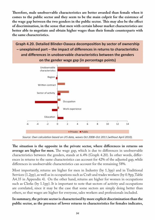
94

Therefore, male unobservable characteristics are better awarded than female when it comes to the public sector and they seem to be the main culprit for the existence of the wage gap between the two genders in the public sector. This may also be the effect of discrimination, in the sense that men with certain labour market characteristics are better able to negotiate and obtain higher wages than their female counterparts with the same characteristics.

Graph 4.20. Detailed Blinder-Oaxaca decomposition by sector of ownership – unexplained part – the impact of differences in returns to characteristics

and differences in unobservable characteristics between the genders on the gender wage gap (in percentage points)

-6 -4 -2 0 2 4 6 8 10 12 14

Educa�on

Work experience

Occupa�on

Sector of ac�vity

Wri�en contract

Region

Unobservablecharacteris�cs

Private Public

Source: Own calculation based on LFS data, waves Oct 2008–Oct 2011 (without April 2010).

The situation is the opposite in the private sector, where differences in returns on average are higher for men. The wage gap, which is due to differences in unobservable characteristics between the genders, stands at 6.4% (Graph 4.20). In other words, differ-ences in returns to the same characteristics can account for 42% of the adjusted gap, while differences in unobservable characteristics can account for the remaining 58%.

Most importantly, returns are higher for men in Industry (by 1.3pp) and in Traditional Services (1.2pp), as well as in occupations such as Craft and trades workers (by 0.9pp, Table A4.35 in Appendix 4). On the other hand, returns are higher for women in occupations such as Clerks (by 1.1pp). It is important to note that sectors of activity and occupations are correlated, since it may be the case that some sectors are simply doing better than others, so that wages are higher for everyone, sales workers and professionals included.

In summary, the private sector is characterised by more explicit discrimination than the public sector, as the presence of lower returns to characteristics for females indicates,

95

but this could also be because there are more sectors in the private sector, so the wage dispersion is wider, and it may be very sector specific, rather than due to the fact that private employers discriminate more.

Differences along the wage distribution in the public vs. the private sector

In this section we analyse the wage gap at the different ponts of the wage distribution in the public and private sectors separately. We split the sample into five wage brackets (quintiles) and compare differences in wages between men and women within these wage quintiles43.

In the public sector, the unadjusted gap is the lowest at the top (among the top 20% of all wages) and the bottom (among the lowest 20% of all wages) parts of the wage distribution (2.3% and 2.4% respectively) and it is the highest in the middle parts of the distribution (4.6%, 4.0% and 4.6 for the 2nd, 3rd and 4th quintile). On the other hand, the adjusted wage gap is distributed slightly more evenly across the wage distribution, since differences in characteristics have the highest impact exactly at the top and the bottom parts of the distribution. Therefore, once we correct for these differences, the wage gap increases both at the bottom and the top of the wage distribution (Graph 4.21).

At both the top and the bottom of the wage distribution in the public sector, female labour market characteristics are better than male, so they underestimate the true gap. The most important characteristic at the top of the wage distribution, which underestimates the wage gap, is women’s higher frequency among Professionals and the higher share of women with tertiary education within this group. The female advantage in characteristics at the bottom of the wage distribution is mainly caused by the lower frequency of women among the low skill Elementary occupations, as well as their lower share in employment in East and South Serbia, where wages are the lowest in the country (Table A4.37 in Appendix 4). This is very intuitive, given the labour market trends in Serbia, where women with the worst skills often self-select out of the labour force because they cannot earn more than their reservation wage. On the other hand, women need better labour market characteristics to be able to enter into the top paid positions in the public sector than men do.

In the middle of the wage distribution (within the 2nd, 3rd and 4th quintiles), women still have better characteristics than men, but to a lesser extent (the explained part of the gap is 0.6, 0.5 and 0.7 respectively). The most important advantage of women within the 2nd and 3rd quintiles is their higher frequency among Technicians, while within the 4th quintile, women are more likely to have tertiary education than men (Table A4.37 in Appendix 4).

43 We drop the dummy variables for year effects in the BO decomposition analysis. Our preliminary analysis showed a significant impact of time effects on the explained part of the gap, which is impossible to interpret, due to the variation in the definition of the wage variable throughout the years. Namely, the interpretation of this coefficient would compare par-ticipation of men and women in survey waves and interpret the differences as higher participation in years where the wages were higher. As already discussed in section 3.5 of our analysis, there are some methodological issues with comparisons of wage levels across years, so the impact of this variable on the explained part cannot be interpreted.

96

Graph 4.21: Unadjusted and adjusted pay gap at different points in the wagedistribution for public (left panel) and private sector (right panel)

2,4%

4,6%4,0%

4,6%

2,3%

4,0%

5,2% 4,6%

5,3%4,6%

0%

1%

2%

3%

4%

5%

6%

1st 2nd 3rd 4th 5th

Public sector

unadjusted gap adjusted gap

3,3%

9,4%12,7%

11,8% 10,4%5,5%9,3%

12,3%

12,2%14,0%

0%

5%

10%

15%

1st 2nd 3rd 4th 5th

Private sector

unadjusted gap adjusted gap

Source: Own calculation based on LFS data, waves Oct 2008–Oct 2011 (without April 2010).

A somewhat different trend emerges in the private sector. The unadjusted gap is the lowest (3.3%) at the bottom quintile of the wage distribution (within the lowest 20% of all wages) and it rises until the middle of the distribution, where it reaches its peak of 12.3% and then drops to 10.4% at the top of the wage distribution (within the highest 20% of all wages).

Differences in labour market characteristics between the genders, similarly to the public sector, are most pronounced at the top and bottom parts of the wage distribution (Table A4.38 in Appendix 4). The explained part of the gap is the highest at the top and the bottom of the wage distribution (3.6pp vs. 2.2pp respectively), while it is close to zero in the middle of the distribution (it is 0.4pp or lower for all three quintiles).

The most important characteristic at the top of the wage distribution is the better overall education of women. The female advantage at the bottom of the wage distribution is mainly caused by the fact that women more often have written contracts than men, i.e. they are less likely to work in the informal sector (Table A4.39 in Appendix 4). This is rather intuitive, as female labour supply is more wage elastic than male (because they choose between reproductive work, leisure and paid work, while men choose between leisure and paid work only), so women are more likely to select away from employment when wages are too low. Furthermore, women are more concerned with the quality of employment, so as second earners in the household they can “afford” to self-select away from precarious employment without written contracts (see literature review for details). On the other hand, and similarly to the trends observed in the public sector, women need better labour market characteristics to be able to enter into the top paid positions in the private sector than men do.

Differences in characteristics affect the adjusted wage gap differently across the quintiles: while it is still the lowest at the bottom part of the distribution, it is the highest at the top of the distribution, suggesting a glass ceiling effect, which means that it is more difficult for women to access the best paid positions in the private sector.

97

5. Gender Pay Gap in Macedonia

5.1 Labour market trends in Macedonia

5.1.1 Main labour market indicators

Female employment rate in Macedonia is significantly lower than male. Employment gap between the genders stood at an average of -18.6 percentage points during the analysed period (Q4 2008 - Q4 2011). Since female unemployment rate is only 0.8 percentage points below male, the observed gap in employment is mostly a reflection of substantial female inactivity, which is by 26.8 percentage points higher than male (Graph 5.1).

Graph 5.1: Main labour market indicators, Q4 2008 – Q4 2011

32,2345 33,356435,4912 34,2590

51,4247 51,835653,8586 52,5139

30,00

35,00

40,00

45,00

50,00

55,00

60,00

Q4 2008 Q4 2009 Q4 2010 Q4 2011

Employment rate

Female Male

34,8146

32,2087

31,7546

32,521832,9340 32,8860

30,852031,4964

30,00

31,00

32,00

33,00

34,00

35,00

36,00

Q4 2008 Q4 2009 Q4 2010 Q4 2011

Unemployment rate

Female Male

50,5494 50,7955 47,9947 49,2294

23,3220 22,7648 22,1112 23,3413

,00

10,00

20,00

30,00

40,00

50,00

60,00

Q4 2008 Q4 2009 Q4 2010 Q4 2011

Inac�vity rate

Female Male

Source: Own calculation based on the LFS data, waves Q4 2008–Q4 2011.

Although the global economic crisis hit Macedonia during the analysed period, no signifi-cant changes in the main labour market indicators for either gender have been observed. Gender gap in employment decreased only slightly – by 1 percentage point, as female employment rate grew by 2.1 and male by 1.1 percentage points. According to World Bank (2011), Macedonia experienced a small employment contraction, or even expanded employment during the crisis relative to its GDP fall (World Bank 2011, p.27).

Female unemployment rate decreased by 0.9 percentage points more than male (albeit from a higher level), while female inactivity rate fell by 1.3 percentage points and male remained at the same level (Graph 5.1). In fact, Macedonia is the only ECA country where unemployment decreased during the crisis (World Bank 2011, p.27).

The fact that women increased their labour market participation in Macedonia during the economic crisis could be understood as a coping mechanism of households facing income shocks – adding a family member to the labour market or replacing a family member who lost their employment. The fact that the overall employment rate did not increase substantially and that there were some changes between types of employment indicates

98

that labour churning44 may have been a significant characteristic of labour market adjust-ment to the crisis. However, without the analysis of flows in and out of employment, we cannot see whether people switched to jobs of worse quality. The fact that we observe a small increase in self-employment rates during the crisis (by 0.3 percentage points among women and 1.4 among men, Graph 5.3) may indicate that the recession pushed people into self-employment out of economic necessity (rather than market opportunity), which would certainly represent cases of last resort employment of almost certainly worse quality than wage employment. At the same time, an active labour market policy implemented by the Macedonian government during the period, which focused on self-employment, may have partially affected these trends45.

Finally, it is important to recognise demand side constraints (i.e. unavailability of additional work), which are particularly pertinent during an economic downturn and which may have limited further increases in female employment.

Mojsoska-Blaževski (2011) suggests a possibility that the crisis did not have a strong impact on the Macedonian labour market because government reform of labour taxes may have offered enough financial space to companies to keep their workers (p.84). Namely, Macedonia reduced social contributions from 32 to 26.9 percent of gross wages in 2009, essentially reducing the cost to hire or keep workers (World Bank 2011, p.14). The effect of the crisis on job loss may have also been reduced because of rigid regulations on firing workers, which made it very difficult for companies to reduce numbers of employees.

When we disaggregate the main labour market indicators by level of education, the gender employment gap is the highest among individuals who only completed primary school. The gap amounts to 23.6 percentage points in comparison to 12.7 for those who completed secondary and 7.8 for those with tertiary education (Graph 5.2, left panel).

Employment gap among those with primary and secondary education is caused by the lower activity of the low-skilled women (39.4 and 17.2 percentage points respectively; Table A5.1 in Appendix 5).46 At the same time, gender gap in unemployment is not high among the low-skill cohorts of the population (-0.6 and 1.4 percentage points respectively). This indicates that a large portion of women with low educational attainment choose not to supply their labour to the market. According to a World Bank (2008) study, the majority of inactive women stated they wanted to work but felt discouraged by the current situation in the labour market so they stopped searching for work altogether.

On the other hand, the gender employment gap among individuals with the highest edu-cational attainment is mainly due to higher unemployment among women than among men (unemployment gap amounts to 7.3 percentage points) and to a lesser extent due to higher female inactivity (inactivity gap amounts to 2.4 percentage points). This suggests

44 Changes in labour market status or type of employment, such as episodes of wife entering labour market as husband exits or an individual switching from wage employment to last resort self-employment, which may not necessarily be visible at the level of average labour market indicators.

45 In 2011, 950 persons started a business through this programme, out of which 340 females.

46 Appendix 5 - appendix to this chapter with supporting data referenced throughout, is available online only, at www.fren.org.rs/node/220.

99

that women with tertiary education are a lot more likely to supply their labour than women with less education. The fact that their unemployment is higher than that of men with tertiary education may point to discrimination of women by employers at the point of job entry and/or that male unobservable characteristics are more valued by employers than female47. However, women with tertiary education seem to be more hopeful about find-ing employment than women with lower educational attainment, so they are more likely to actively seek work rather than withdraw into inactivity. An interesting finding emerges from a World Bank (2008) study. Namely, both women and men in Macedonia are discouraged about finding employment because they “lack personal connections” and are not affiliated with the political parties in power. Their findings show that this attitude prevailed regardless of these individuals’ educational attainment. However, if we consider that higher educational attainment also improves individuals’ social capital and possibly even their access to political parties, we may conclude that both women and men with better educational attainment are less likely to be discouraged about their employment prospects.

Graph 5.2: Employment rate by… ...gender and level of education (15-64) …gender and age (15-64)

16,3

42,8

65,9

39,9

55,5

73,7

0

10

20

30

40

50

60

70

80

Primary Secondary Ter�ary

Female Male

10,4

45

2319,2

65,8

46,9

0

10

20

30

40

50

60

70

15-24 25-54 55-64

Female Male

Source: Own calculation based on the LFS data, waves Q4 2008–Q4 2011.

Observed by age (Graph 5.2, right panel), the employment gap is the highest among the oldest members of the labour force (age group 55-64). Their gender employment gap (36.1 percentage points) is significantly wider than the gap among the prime age group (20.8pp). On the other hand, gender employment gap is the lowest among youth (8.7 percentage points). We can probably explain this by the changing role of female household members as well as by the fact that new generations of females are more educated than older ones, which leads to declining employment and participation gaps between the genders. At the same time, inactivity is high among youth of both genders, mostly due to school/university attendance.

47 Since unemployment as defined in the LFS covers only those individuals who are actively seeking a job, rather than those who may officially register as unemployed in order to claim benefits, we are not concerned about the perverse incentives which may motivate women as second earners to declare themselves as unemployed.

100

Gender employment gap for all analysed age groups is mainly caused by variation in inactiv-ity rates between the genders, which is most pronounced among the oldest age cohort (36.1 percentage points; Table A5.2 in Appendix 5). This is probably due to the fact that women retire earlier than men and require less work experience to qualify for retiring. However, female unemployment rate for the oldest age group (55-64) is also higher than male (by 5.5 percentage points), which suggests that elderly women in particular have more difficulty in finding employment than men, i.e. that the effect of employer discrimination and/or unob-servable differences in labour market characteristics may be especially pronounced among women in the age bracket 55-64. For the other two (younger) age groups (15-24 and 25-54), unemployment rates are only slightly higher among women (by 3.4 and 1.7 percentage points respectively) (Table A5.2 in Appendix 5). Therefore, the most senior group of working age women seems to be particularly vulnerable in the labour market.

5.1.2 Type of employment

Compared to men, women in Macedonia are more often in wage employment than in self-employment (77.1% compared to 70.1% of men) (Graph 5.3). From the perspective of market economies, this could be argued as surprising since it is mostly men who prefer wage employment due to greater chances of promotion (e.g. they are not exposed to the glass ceiling effect) and because women may favour self-employment due to greater opportunities for flexible working arrangements. Yet, in transition countries, the op-posite mechanism seems to be at work, since women on average have more secure jobs, because of their more frequent employment in the public sector (public administration, health and education).

Due to serious demand-side constraints in the labour market, such as high unemployment and low levels of generation of new jobs, self-employment could be characterised as employment of last resort (due to lack of wage employment opportunities). The fact that self-employment among men increased by 1.4 percentage points during the crisis may support this argument (Graph 5.3, left panel). At the same time, some of the prerequisites for self-employment are initial capital for investment and informal networks, both of which may be more accessible to men than to women.

Although a higher percentage of employed women than employed men are in wage em-ployment, women are a minority in total wage employment (40.9% of the total). The fact that fewer women work overall could imply that women are more likely than men to choose employment only if it is better quality (including family-friendly working hours) and lower risk (i.e. wage employment), whereas men are less wage elastic and will work regardless of what type of work is available to them. The fact that women work less often as self-employed (8.4% vs. 24.2% of men) speaks in favour of this proposition (Graph 5.3).

Women are also found to more frequently work as unpaid family members (14.5% of all employed women, compared to 5.7% of men), most often in agriculture.

Structure of the employed does not change significantly between 2008 and 2011. As dis-cussed previously, it seems that the overall increase in employment rate for both genders is

101

due to the rise in self-employment and stagnation in all other categories, which may be last resort employment, i.e. a coping mechanism against negative income shocks.

Graph 5.3: Structure of employment by type and gender (15-64)… …and share of women by type of employment (15-64)

77,1 70,1 78 72,5 77,7 70,9

8,4 24,2 8,1 22,4 9,1 24,1

14,5 5,7 14 5,1 13,2 5

0%

20%

40%

60%

80%

100%

Female Male Female Male Female Male

Average for allwaves

Q4 2008 Q4 2011

Wage-employed Self-employed Unpaid family members

40,9

17,9

61,4

39,6

18

62,7

41

19,4

62,6

0 10 20 30 40 50 60 70

Wage-employed

Self-employed

Unpaid family members

Q4 2011 Q4 2008 Average for all wages

Source: Own calculation based on the LFS data, waves Q4 2008–Q4 2011.

Women with primary educational attainment are predominantly employed as unpaid contributing family members. They make half of the total number of employed women with primary education only, compared to 14.5% on average at other levels of educational attainment (Table A5.3 in Appendix 5). Only 39.5% of women with primary education are in wage employment (compared to 77% for all women). Among men with primary educa-tion, there is a high share of the self-employed (42.4% compared to 24.2% for all men), and a significantly lower number of those in wage employment (45% vs. 70.1% for all men). These data also seem to support our proposition that much of the self-employment in Macedonia is employment of last resort.

Since the self-employed and unpaid family members with low educational attainment frequently work in agriculture, one explanation of the variability in types of employment observed among men and women may be that men and women frequently work on one farm. In that case, men may be more likely to answer that they are self-employed (head of the household), while women who work with them answer that they are unpaid contribut-ing family members. This points to unequal access of rural women to resources, compared to rural men.

More education increases the share of wage employment among both women and men. Wage employment on average represents over 80% of all types of employment for individu-als with secondary education and 85% for those with tertiary (Table A5.3 in Appendix 5).

Disaggregation by age groups indicates that the presence of women among unpaid family members rises with age (Table A5.4 in Appendix 5). Among the 55-64 age group 90% of all unpaid family members are women. This indicates another dimension of labour market vulnerability of elderly women apart from inactivity – they are very often unpaid for their work.

102

5.1.3 Unadjusted gender wage gap and labour market characteristics

In this section we focus on wage employment only, which is the sub-sample of employees that we use in our regresion analysis. We describe wage characteristics for men and women, gender differences in wages as well as the structure of wage employment.

The sample that we use throughout our analysis in this chapter consists of 19,737 indi-viduals (8,107 women and 11,630 men) for whom we observe wages in the LFS in the period from the 4th quarter of 2008 to the 4th quarer of 2011.48 The base sample includes individuals in the age group 15-64, who work full-time either in the public or the private sector49 and receive positive wages from employment.50 We exclude those in training or formal education, as well as the self-employed and/or unpaid family members.51

Gender wage gap is analysed at the level of real log hourly wages, deflated using the Con-sumer Price Index (CPI), with October 2008 as the baseline.

Table 5.4: Descriptive statistics of male and female wages (15-64)

Hourly log wages Unadjusted

Female Male wage gap (%)

1st quintile 3.479 3.594 11.5***2nd quintile 3.801 3.957 15.6***3rd quintile 4.026 4.221 19.5***4th quintile 4.374 4.496 12.2***5th quintile 4.808 4.911 10.3***

Mean 4.088 4.222 13.4***Sample 8,107 11,630Source: Own calculation based on the LFS data, waves Q4 2008 – Q4 2011.

The mean unadjusted wage gap in Macedonia is 13.4% in favour of men. However, the gender gap differs significantly across the wage distribution. In order to analyse these dif-ferences we split the female and male samples into five wage brackets (quintiles) and then compare the average wage of men and women within each of the quintiles. The gap is the lowest in the 1st and the 5th quintile and the highest in the middle of the distribution. At the bottom of the wage distribution female wages are on average 11.5% lower than male. The gap grows to 15.6% in the 2nd and to 19.5% in the 3rd quintile of the wage distribu-tion, where it reaches its maximum. In the higher wage quintiles, the gap drops again, first to 12.2% in the 4th quintile and then to 10.3% at the top quintile of the wage distribution

48 LFS in Macedonia is implemented twice per year, in the second (Q2) and fourth quarter (Q4).

49 We exclude those whose answer to the ownership question in the survey is „other.“

50 162 cases with zero wages are excluded from the analysis. We further exclude those workers with missing values for tenure (22 cases) and sector of ownership (176 cases in which sector of ownership is “other”, rather than public or private).

51 We will later test our results for robustness separately for public and private sector workers.

103

(Table 5.4; for a more detailed discussion on gender gap per quintiles see section 5.2.2 of this chapter).

In this section we disaggregate the average unadjusted gender wage gap and average female wages by level of education, tenure, occupation, sector of activity, type of ownership and type of working contract.52 Since labour market characteristics of employed women vary in comparison to those of employed men, we also contrast these different gender wage gaps and female wage levels against variations in labour market characteristics of both genders. This is a necessary step because in the next section we will reweigh the average differences between men and women in each cohort and adjust the gender wage gap accordingly, based on these variations in labour market characteristics. That step will ensure that we compare wages between a man and a woman with exactly the same labour market characteristics (instead of the average employed woman against an average employed man, who have very different labour market characteristics). The data on the unadjusted gender wage gap and labour market characteristics are summarised in Graphs 5.5-5.7 below.

Graph 5.5: Unadjusted gender wage gaps,female log wages and employment gaps, by level of education (15-64)

Primary or Lower

Secondary

Ter�ary

3,4

3,6

3,8

4

4,2

4,4

4,6

4,8

5

5 10 15 20 25 30

Fem

ale

log

wag

es

Unadjusted wage gap (%)

Source: Own calculation based on the LFS data, waves Q4 2008–Q4 2011.Notes: 1) Size of the circles indicates the differences in the frequency of male vs. female employment by level of education. Lighter circles represent those characteristics which can be found more frequently among employed women than among employed men (e.g. employed women more frequently have tertiary educa-tion than employed men), while darker circles represent those characteristics which can be found more fre-quently among employed men (e.g. employed men more frequently have secondary education than employed women). The size (surface) of the circle shows the extent of this difference between the genders by that

particular labour market characterisic.2) The data used for this graph can be found in Table A5.5 in Appendix 5.

52 While graphs on education, occupation and sector of activity are shown below, data on years of tenure, type of ownership and type of working contract can be found in Appendix 5.

104

Educational structure of employed women is much more favourable than that of employed men: 28.1% of women in wage employment have tertiary education (compared to 20.6% of employed men), while 12.7% of them have primary education only (compared to 17.7% of employed men) (Graph 5.5 and Table A5.5 in Appendix 5).

Therefore, the higher positioned the circle on the graph, the higher the pay for women with that particular characteristic represented by the circle. Graph 5.5, not surprisingly, shows that women with tertiary education earn more than women with secondary and primary education (the circle for tertiary education is higher positioned on the y-axis).

Graph 5.5 shows that the highest wage gap between the genders can be found among those with primary education, closely followed by secondary. Therefore, the unadjusted gender wage gap shrinks with the level of education. The difference in the average wage between women and men with tertiary education is significantly lower than between women and men with lower levels of education – 10.4% in comparison to 20.1% for those with secondary and 22.3% for those with primary.

When it comes to tenure53 with current employer (Table A5.6 in Appendix 5), the lowest difference in the average wage (only 2.1%, not statistically significant) was observed among those with over 20 years with the same employer. This trend could reflect the greater gender equality at the start of career (in socialism) for those with over 20 years of experience. For those individuals with lower tenure, the difference in the average wage between the genders is higher (against women), and varies between 14 and 17%. This might imply that young women in particularly experience wage discrimination in the labour market, possibly due to their childbearing responsibilities. At the same time, the tenure structure is approximately similar for both genders, with slightly lower average tenure of women (10.3 years vs. 11.1 for men). This difference is due to higher participation of men in the group with tenure longer than 20 years (Table A5.6 in Appendix 5).

When we disaggregate the data by occupation, we observe a clustering of occupations that require lower skills and pay lower wages vs. occupations that require higher skills and pay higher wages (Graph 5.6). The unadjusted wage gap is wider in occupations that also have lower female wages (the lower circles to the right of the x-axis).

Plant and machine operators and Service and sales workers are two sectors characterised by the largest unadjusted gender wage gap among all occupations (gap is 36.6% and 29% respectively), as well as the lowest female wages. Furthermore, women can be found more frequently in these two occupations than men and these are the sectors in which women work more often than in the other two low-skill, low wage occupations (Elementary oc-cupations and Craft and trades workers, see Table A5.7 in Appendix 5). Namely, more than one third of all women in wage employment work in these two sectors (21.4% and 17.8% of them respectively). The fact that the gap is the highest among Plant and machine opera-tors may be because female workers predominately work in the textile industry, which has by far the lowest wages in the country (Mojsoska-Blaževski, 2011). In conclusion, among the low-skill, low wage occupations, those in which women can be found more frequently also have larger wage gaps.53 We use tenure as a proxy variable for experience, since we do not have data on total work experience.

105

Graph 5.6: Unadjusted gender wage gaps,female log wages and employment gaps, by occupation (15-64)

Senior officials and managers

Professionals

Tehnicians and Associate

ProfessionalsClerks

Service and sales workers

Cra� and Trade Workers

Plant and machine operators

Elementary occupa�ons

33,2

3,4

3,6

3,8

4

4,2

4,4

4,6

4,8

5

-10 0 10 20 30 40 50

Fem

ale

log

wag

es

Unadjusted wage gap (%)

Source: Own calculation based on the LFS data, waves Q4 2008–Q4 2011.Footnotes: (a) Professionals include armed forces. (b) Technicians and associate professionals include skilled

agricultural workers.Notes: 1) Size (surface) of the circles indicates the differences in the frequency of male vs. female employment by occupation. Lighter circles represent those occupations in which women can be found more frequently than men (e.g. women can be found more frequently working as Clerks than men), while darker circles represent those occupations in which men are employed more frequently (e.g. men can be found more frequently work-ing as Senior officials and managers than women). The size of the circle shows the extent of this difference in

gender frequencies within each occupation.2) The data used for this graph can be found in Table A5.7 in Appendix 5.

The unadjusted wage gap is a lot smaller among high-skill, high wage occupations. In three of the four of these occupations, women can be found more frequently than men (three of the four circles in the upper-left part of the Graph 5.6 are lighter). Interestingly enough, of all the high-skill, high wage occupations, women can be found least frequently among Senior officials and managers (the only darker circle), who along with Professionals have the highest wages. Namely, among Senior officials and managers there are twice as many men as women, possibly suggesting a “glass ceiling” for women, who, although their overall educational structure is better than male, cannot access the top positions, which pay the highest wages. Of course, a supply side reason for this could be that women select away from positions with greater responsibility due to different preferences in comparison to men. For those women who do access Senior officials and managers, they receive wages which are on average by 9%54 lower than those for male Senior officials and managers.

Among Clerks, women on average receive the same wages as men (i.e. insignificantly higher, by 1.5%) and they take up the majority of all positions. This is probably due to a large frequency of female employment in the public sector. Similarly, the lowest positive 54 This difference is only marginally significant, at the 0.1 level, probably due to the small sample of managers.

106

difference in the average wage between the genders (by 3.6%) is among Professionals, where women occupy approximately one half of all positions.55

Graph 5.7: Unadjusted gender wage gaps,female log wages and employment gaps, by sector of activity (15-64)

Agriculture

Industry

Tradi�onal Services

Modern Services

Public Services

33,2

3,4

3,6

3,8

4

4,2

4,4

4,6

4,8

-15 -5 5 15 25 35

Fem

ale

log

wag

es

Unadjusted wage gap (%)

Source: Own calculation based on the LFS data, waves Q4 2008–Q4 2011.Footnotes: (a) Traditional services: Trade, HORECA, Transport. (b) Modern services: Communication, Financial intermediation, Real estate, Experts. (c) Public services: Public administration, Education,

Health, Social service activities, ET organisations.Notes: 1) Size (surface) of the circles indicates the differences in the frequency of male vs. female employment by sector of activity. Lighter circles represent those sectors in which women can be found more frequently than men (e.g. women can be found working in Public services more fre-quently than men), while darker circles represent those sectors in which men are employed more frequently (e.g. men can be found working in Industry more frequently than women). The size (surface) of the circle shows the extent of this difference in gender frequencies within each sector.

2) The data used for this graph can be found in Table A5.8 in Appendix 5.

When it comes to sectors of activity, the largest unadjusted wage gap (i.e. difference in the average wage) is observed in Industry (28.9%), followed by Traditional services (18.5%). These sectors are also the sectors – apart from Agriculture – with the lowest wages (low-skill, low wage sectors, in which men work more frequently than women) (darker circles in Graph 5.7)).

In Agriculture, the wage gap is lower than average (10.2% vs. average 13.4%). However, this is a sector characterised by the lowest wages, so a government imposed minimum wage (which applies to both genders) could be the reason why the gap is not very large (Graph 5.7).

55 Since this group includes army officers, numbering around 40,000 men and on ly 1,000 women, women actually make the majority in this group when we exclude the army.

107

Women work more frequently than men in high wage, high-skill sectors, such as Modern services and Public services. This is consistent with the fact that in Macedonia high-skilled women tend to work, while low-skilled women stay out of the labour force. However, these two sectors differ significantly in the size of the unadjusted wage gap. Modern services, where both fewer men and women work (around 8% of women and 6% of men) is the only sector where women on average receive higher wages than men (by 9%). On the other hand, in Public services, where almost one third of women and one quarter of men work, women earn 9% less than men.

When we analyse wage data according to whether the sector is in public or private owner-ship, a couple of interesting trends emerge (data can be found in Table A5.9 in Appendix 5). There is a clear cleavage according to ownership, so that we observe a substantially higher unadjusted pay gap (i.e. larger difference in the average wage) in the private than in the public sector (17.7 vs. 4%). Although it may seem attractive to rush to the conclu-sion that the public sector discriminates against women less than the private sector, we must also keep in mind that workers in the public sector are on average better educated and that there is a significantly larger portion of high-skilled workers among them. As we have seen from Graphs 5.5-5.7, the pay gap shrinks as education and skill levels grow. Furthermore, although much of the transition literature points to the fact that women dominate the public sector because of the traditionally female occupations it covers (such as education and health), this does not seem to be the case in Macedonia. Although women can be found to work in the public sector more frequently than in the private sector, the share of women in the public sector compared to all employed women is almost equal to the share of men (in addition, more men work in the economy as a whole, so their numbers in the public sector by far exceed female). Women in Macedonia could have had a somewhat lower access to public employment than in the neighbouring countries, due to affirmative action to have the large-sized Albanian ethnic minority equally represented in the public sector (regardless of gender).

The difference in the average wage between the genders is more pronounced among work-ers with permanent contracts – 14.7% vs. 12.8% among those with temporary contracts. Yet, women also have permanent contracts more often than men do (88.6 vs. 84.3% of all wage employees) (Table A5.10 in Appendix 5).

We also analysed gender differences between workers in the informal and formal sector of the economy, i.e. those who have a written contract with their employers vs. those who do not. We found that the percentage of women working without a written contract is lower than the percentage of men by 4 percentage points (4.4% in comparison to 8.4%). When working without a written contract, the pay gap between women and men is even higher – 20.8% as opposed to 13.7% when there is a written contract. However, we do not include these data in our econometric analysis since the data on written contract were not available for the 4th quarter of 2008.

108

5.2 Understanding the gap (econometric analysis)

As we have shown in the previous section, the two genders differ significantly according to characteristics and skill levels of women and men who work. Therefore, in this section we adjust the gender wage gap to reflect these differences in characteristics. In that sense, we move away from a simple calculation of the difference in the average wage between an average employed man and an average employed woman, i.e. the unadjusted pay gap, and reweigh it by labour market characteristics of each employed individual. We then get the adjusted gender wage gap, i.e. the true wage gap between the genders.

The purpose of this section is to throw more light on the reasons why the gender pay gap exists and persists in the Macedonian labour market. Identifying factors which explain the gender pay gap is extremely important from the policy perspective, because only knowing what affects the gender pay gap can help policy makers design measures to tackle it.

5.2.1 Mincer wage equations and the Blinder-Oaxaca decomposition

Table 5.8 shows estimation results of four different specifications (S1 to S4) of the Mince-rian wage regression. Robustness checks (population subgroups of 19-64 and 19-59 years of age; wages with and without extreme values and inclusion of workers with zero wages) are reported in Table A5.12 of Appendix 5. In all of the reported specifications, standard errors are corrected for heteroskedasticity using the robust (“sandwich”) estimator. Our dependent variable is log hourly real wage.56

Table 5.8: Mincer wage regressions (Specifications S1 to S4)

Variable S1 S2 S3 S4Female -0.134*** -0.175*** -0.175*** -0.179***

(0.007) (0.006) (0.006) (0.006)Education and tenure Yes Yes Yes

Time fixed effects Yes YesWork related variables (1) Yes

Sample 19,738 19,738 19,738 19,738Adjusted R-square 0.018 0.30 0.31 0.41

Log Likelihood -13557 -10268 -10054 -8514Source: Own calculation based on the LFS data, waves Q4 2008–Q4 2011.Robust standard errors in parentheses. Notes: * p<.1; ** p<.05; *** p<.01

(1) Occupation (ISCO), Sector of activity (NACE), Ownership (public/private), Type of contract (temporary/permanent; written/non-written).

56 Wages in the 4th quarter of 2008 are reported as exact wage amounts, while in the consecutive waves respondents select a wage bracket for their earnings. In 2009 and 2010 there were 10, and in 2011 there were 11 wage brackets. Wages are transformed from nominal to real wages using the Consumer Price Index (CPI) with the 4th quarter of 2008 as baseline. The data on CPI were taken directly from the Macedonian National Statistical Office (Državen zavod za statistika) website.

109

The coefficient for female in specification S1, where female is the only explanatory variable, represents the unadjusted gender pay gap. Coefficients in specifications S2-S4 represent the gender pay gap adjusted for variables marked with x. Coefficients for all explanatory variables in the Mincerian wage equation are reported in Table A5.11 of Appendix 5.

The specification S1 estimates that women in Macedonia, on average, have 13.4% lower hourly wages than men (this is also what we conclude from analysis of the unadjusted gender wage gap presented in the previous section).

This gap in earnings between the genders widens to 17.5% when we account for educa-tion and tenure (specification S2). Coefficients for the two education dummy variables measuring secondary and tertiary education are positive and rising with level of education (elementary education is the omitted category), returns to education increase with educa-tion, such that those with secondary and tertiary education have respectively 7.6% and 26% higher wages than individuals with elementary education only. Similarly, the coefficient for tenure is positive, showing that the wage increases with the time spent working for the same employer (See Table A5.11 in Appendix 5).57

Accounting for time fixed effects (specification S3) does not change the coefficient for gen-der (nor for education and tenure), suggesting that the specification is robust over time. The gender wage gap increases further, albeit slightly – from 17.5 to 17.9%, when additional job characteristics, such as sector of activity, occupation and type of contract, are taken into account (specification S4). Coefficients for education stay positive and rising with the level of education when we include job characteristics into the equation, but returns to education become substantially lower due to their correlation with job characteristics58 (see Table A5.11 in Appendix 5). In other words, returns to education are overestimated in the previous specifications, because we exclude job characteristics.

The estimates from Mincerian equations can be summarised in the basic Blinder-Oaxaca decomposition, where the average log hourly wage is decomposed into the explained part (due to differences in workers’ personal and job characteristics) and the unexplained part (differences in returns to the same personal characteristics and differences due to unob-servable differences in personal characteristics) (Table 5.9).

From the Mincerian wage estimates and the descriptive analysis of the unadjusted pay gap in the previous section, we have seen that on average, employed women have 13.4% lower hourly wages than men. However, unlike the trends we observe in the Western economies (see literature review), the differences in labour market characteristics between men and women (e.g. education, tenure, job characteristics) cannot explain the gender wage gap in Macedonia. In fact, exactly the opposite effect is in place. When personal labour market characteristics are taken into account, the gap widens. This can be explained by the fact that an average employed woman in Macedonia has better labour market characteristics than an average employed man. This occurs because a significant portion of low-skilled women 57 The variable measuring total working experience was not available for Macedonia.

58 Most importantly, working as a professional correlates positively with tertiary education (0.66) and negatively with secondary education (-0.46); working in a state/socially owned company correlates positively with tenure (0.35) and work-ing in public services (public administration, education, health, etc) correlates positively with tertiary education (0.35).

110

stay out of the labour market, meaning that they self-select out of employment due to the low opportunity cost59 of not working (higher female reservation wage at low-skilled level). This may be due to, for example, care for children and the elderly, as well as presence of the more traditional household models where women are exclusively in charge of reproduc-tive work (especially among the less educated households). It could also be the case that discrimination of low-skilled women occurs at the point of entry into the labour market, so that they do not have many opportunities to obtain work.

Although female labour supply decisions are beyond the scope of this research,60 it is important to keep in mind that this greatly impacts the actual gender wage gap, since non-employment of low-skilled women increases the wage of the average working woman and therefore hides the real gender wage gap in the economy. In other words, if women who worked had the same labour market characteristics as employed men, the gender wage gap would be substantially larger. When the gender wage gap is adjusted for personal labour market characteristics (i.e. if the average working man and working woman were to have the same educational level, tenure and job characteristics), it increases from 13.4% to 17.9%.

Table 5.9 Blinder-Oaxaca decomposition – main results (Specification S4)

Coefficients Standard errors

Men (average log hourly wage) 4.222*** (0.004)

Women (average log hourly wage) 4.088*** (0.005)

Difference (unadjusted gender pay gap) 0.134*** (0.007)

Explained part -0.045*** (0.005)

Unexplained part (adjusted gender pay gap) 0.179*** (0.006)Source: Own calculation based on LFS data, waves Q4 2008–Q4 2011.

Robust standard errors in parentheses. Notes: * p<.1; ** p<.05; *** p<.01

Differences in labour market characteristics

Graph 5.10 shows the impact of labour market characteristics on the gender pay gap. What narrows the unadjusted gender pay gap is that employed women on average have higher educational attainment and work more frequently in high-skill, high wage jobs than men do (this is also visible from descriptive statistics presented in the previous section). Moreover, women are better positioned regarding the sector of activity they work in and the type of employment contract they have, meaning that they can more frequently be found working in the better-paid sectors of the economy (e.g. services, and especially Public services). They also hold permanent contracts more frequently than men do (probably precisely due to the fact that they more frequently work in the public sector). 59 This may be further reinforced by the high levels of outmigration and strong reliance of households on remittances from family members working abroad.

60 Although we use Heckman selection correction to correct for self-selection into employment. See section 5.2.4 of this chapter for more details.

111

Graph 5.10: Detailed Blinder-Oaxaca decomposition (in percentage points)

-4 -2 0 2 4 6 8 10 12 14

Educa�on

Tenure

Occupa�on

Sector of ac�vity

Ownership

Type of contract

Unobservablecharacteris�cs

Differences in returns Differences in characteris�cs

Source: Own calculation based on LFS data, waves Q4 2008–Q4 2011.Notes: 1) The darker bars placed on the negative side of the x-axis represent characteristics which underesti-mate the true gap, while the darker bars placed on the positive side overestimate the true gap (lighter bars

refer to differences in returns, which we discuss in the next section). 2) Unobservables are only present under differences in returns, since they represent differences in unobserv-

able characteristics that cannot be measured.3) The data used for this graph can be found in Table A5.13 in Appendix 5.

However, women are worse off than men when it comes to tenure, since theirs is on average lower than male (see section 5.1.3 for details). This is likely the result of a number of fac-tors, including career interruptions due to childbearing, the fact that the average working woman is more educated than the average man (which implies more time in education instead of at work), as well as earlier retirement age. Therefore, gender differences in tenure work in the opposite direction from most of the other personal characteristics, i.e. they make the true gender wage gap seem bigger than it is (albeit slightly; the darker bar for tenure is positive but very small).

We now show the separate contribution of each of these individual labour market characteris-tics to the gender pay gap, since Graph 5.10 only shows grouped effects of education (primary, secondary, and tertiary together), tenure (tenure and tenure squared), time (seven waves of data), occupation (eight categories), and sector of activity (five categories). Separate contribution of each of the individual characteristics can be found in Table A5.14 in Appendix 5.

The unadjusted wage gap is “underestimated” by 1.8pp due to the effect of higher average education of employed women than employed men (Graph 5.10, darker bar). Compared to men, working women have tertiary education more frequently then working men, while men are more frequently found with primary education only (Graph 5.5). Since workers with tertiary education have higher wages, female average wages would be lower (and therefore the wage gap would be higher) if employed women had the same educational characteristics as employed men. Educational differences between the genders can account for 40% of the explained part of the gap.

112

The unadjusted gender wage gap would be higher by 2pp if women had the same occu-pational characteristics as men (Graph 5.10, darker bar). Occupational characteristics ac-count for 44% of the explained part of the gap. However, unlike is the case with education, differences in characteristics between men and women in different occupations operate in different directions: while some make the true wage gap seem larger, others make it seem smaller (see Graph 5.6 for details).

Less frequent presence of women among the highly paid Senior officials and managers (women make only 30% of them) overestimates the wage gap by 0.3pp. On the other hand, lower female than male frequency in managerial positions points to a different type of discrimination – the glass ceiling effect. Another factor that overestimates the wage gap is the higher percentage of women in low pay jobs among Plant and machine opera-tors and Service and sales workers (by 6.6pp and 1.2pp respectively). These characteristics overestimate the gap by 1.1pp and 0.2pp respectively.

At the same time, a higher frequency of women in high pay jobs conducted by Profes-sionals, Technicians and associate professionals and Clerks (by 4pp, 4.7pp and 3.7pp) underestimates the pay gap by 0.9pp, 0.3pp and 0.2pp respectively. Also, the fact that women can less frequently be found in the low pay jobs among Craft and trades workers and Elementary occupations (by 16.3pp and 2.6pp) underestimates the gap by 1.6pp and 0.6pp respectively. In total, occupational differences underestimate the gap (by 2pp), since those characteristics that underestimate the gap prevail over those that overestimate the gap.

The gender pay gap would be higher by 0.7pp if employed women were distributed by sector of activity in the same manner as men (Graph 2.3, darker bar) – sector of activity accounts for around 15% of the explained gap. More specifically, the fact that women less frequently work in low pay jobs in Agriculture (Graph 5.7) underestimates the gap by 0.4pp, while their high frequency in high pay jobs in Modern and Public Services (Graph 5.7) underestimates the gap by 0.2pp and 0.1pp respectively.

The fact that a higher percentage of women (by 4.2pp) have permanent contracts under-estimates the gender pay gap by 0.4pp (permanent contracts entail higher wages than temporary ones): type of contract accounts for 8% of the explained part of the wage gap between the genders.

Since wages grow with tenure, the fact that women on average have less tenure than men overestimates the gender wage gap by 0.2pp (Graph 5.10, darker bar). Therefore, tenure contributes around 4% to the total explained gender pay gap (albeit in the opposite direc-tion from the above factors).

Table 5.11 summarises the above discussion. Overall, better labour market characteristics of women in comparison to men prevail over the worse ones, so that the total unadjusted gender wage gap of 13.4% is an underestimate. This is why it increases to 17.9% when we reweigh the data so that it is possible to compare women and men with exactly the same labour market characteristics. Therefore, we can say that the true gender wage gap is 17.9%.

113

Table 5.11: Detailed Blinder-Oaxaca decomposition – explained part – the impact of differences in characteristics between the genders

on the gender wage gap

High wage jobs Low wage jobs

Higher frequency of women

Tertiary education (-1.1pp)Professionals, technicians and associate profession-

als, Clerks (-1.4pp)Modern(a) and Public

Services(b) sector (-0.3pp)Permanent contract (-0.4pp)

These characteristics make the true gap seem smaller.

Plant and machine operators and Service and sales workers (1.3pp)

These characteristics make the true gap seem larger.

Lower frequency of women

Managers (0.3pp)

Higher tenure (0.2pp)

These characteristics make the true gap seem larger.

Primary and secondary education (-0.7pp)

Craft and trades workers (-1.6pp) and Elementary occupations

(-0.6pp)Agriculture (-0.4pp)

These characteristics make the true gap seem smaller.

Source: Own calculation based on LFS data, waves Q4 2008–Q4 2011. For standard errors see Table A5.14 in Appendix 5.

Note: Numbers in brackets show how much the gap is underestimated or overestimated when not adjusted for the difference in the characteristic. Percentage points shown in brackets show contribution of each char-

acteristic to the adjustment of the total gap.Footnotes: (a) Communication, Financial intermediation, Real estate, Experts

(b) Public administration, Education, Health, Social service qctivities, ET organisations

Differences in returns

In the previous sub-section, we analysed in detail the explained part of the gender pay gap. We looked at the contribution of average personal characteristics of employed women vs. employed men to the observed difference in their wages. In that sense, we assumed the same returns to the same characteristics for both genders, i.e. we assumed that employers would pay the same wage to a woman if she had the same labour market characteristics as a man. The main conclusion that stemmed from that analysis is that if women in Macedonia had the same labour market characteristics as men, the gender pay gap would be 17.9%.

114

In this section of the report, we analyse this unexplained part of the wage differential, i.e., the adjusted gender wage gap. This unexplained, or adjusted, wage gap of 17.9% exists because of: i) labour market discrimination of women, in the sense that there are differ-ences in returns to the same labour market characteristics between the genders, and ii) unobserved heterogeneity of workers’ characteristics, which we were not able to capture through variables such as education, tenure, occupation, etc.

According to the results of the Blinder-Oaxaca decomposition presented in Graph 5.10 (and Table A5.13 in Appendix 5), the largest share of the unexplained part of the wage gap – 69% (12.5% out of 17.9%; Graph 5.10, bar Unobservable characteristics) – stems from unobservable characteristics of workers, i.e. individual characteristics which are important for labour market valuation but go beyond the variables we analyse (such as education, tenure etc.). These could include differences in female and male labour market behaviour which employers reward or punish within the same occupations and sectors of the economy, e.g. that women may be less flexible in terms of working hours or business trips, due to home/reproductive responsibilities; other non-measurable effort- and ability-related variables, as well as labour market frictions. Unfortunately, due to constraints in data availability, these unobserved characteristics are beyond the scope of this analysis.

On the other hand, differences in returns to personal labour market characteristics and choice of occupation can account for 31% of the unexplained wage gap (5.4% out of 17.9%, Graph 5.10). Women, on average, have lower market returns to education, choice of occupation and sector of activity, when these characteristics are treated as one61 (Graph 5.10, red bars). A more detailed decomposition reveals that for some of the labour market characteristics, such as specific occupations (managers, professionals, etc.), male returns are higher than female, while for others, it is exactly the opposite: female returns are higher than male (Table A5.14 in Appendix 5).

The overall differences in wage returns to education account for approximately 3% of the unexplained part (0.6 of the 17.9% gap).62 Investment into tertiary education has higher pay-offs for men than for women (by 0.8 percentage points), which can be explained by the glass ceiling which reduces female opportunities for promotion and their access to top managerial positions. Furthermore, men with tertiary level of education, on average, make 28% higher wages than men with primary level of education, while for women this difference is 21%.63 While differences in returns to secondary education are not statistically significant, women have higher “returns” to primary education than men (by 0.5pp), which

61 For example, the coefficient for education is the sum of the coefficients for primary, secondary and tertiary level of education.

62 The results from the Mincerian wage equation are presented with primary education as the omitted category. However, coefficients for the unexplained part of the gap stemming from the BO decomposition for different levels of education are calculated using the constant deviation contrast transformation. The transformation is based on the series of estimations in which categories (in this case: primary, secondary and tertiary level of education) are used one after another as the base (omitted) category and the restriction that the sum of the coefficients must be equal to zero. Thus the results of the Blinder–Oaxaca decomposition are independent of the choice of the omitted category. This transformation is applied for all the dummy variables representing categorical variables with three or more categories. More details on the transformation can be found in Yun (2005) and Jan (2008).

63 Statistical significance of this difference is confirmed in the BO decomposition.

115

could be explained by the fact that a significant portion of women with primary education self-select out of employment so that the ones who stay remain employed because it pays off for them.

Since Mincerian regression coefficients for tenure are approximately equal for both genders (0.013 for men and 0.011 for women), the BO decomposition does not show any statistical differences in returns to tenure. Therefore, we can conclude that different returns to tenure are not the source of discrimination in Macedonia.

Different returns to the same occupation account for 10% of the unexplained part of the wage gap (1.8 of the 17.9%). However, depending on the occupation, returns are some-times higher for women and at other times for men (controlling for education). Returns are higher for women in the following occupations: Professionals (by 1.6pp), Clerks (by 1.4pp), Technicians and associate professionals (by 0.7%), Managers (by 0.2pp).64

The most outstanding difference in returns to occupation is among Plant and machine operators, where men have higher returns by 3.6pp.65 As we suggest in the previous section, this may be related to the fact that women more often work in the textile industry, which is characterised by the lowest wages in the economy. Other occupations where men have higher returns than women are Service and sales workers (by 1.3pp) and Craft and trades workers (by 0.5pp).

The difference in returns to sector of activity accounts for 17% of the unexplained part of the wage differential (3% of 17.9%) and as such is the highest source of differences in wage returns to labour market characteristics between men and women. More specifically, returns are higher for men in Industry (by 1.5pp), Public Services66 (by 1.1pp) and Tradi-tional Services67 sector (by 0.9pp), while they are higher for women in Modern Services68 (by 0.4pp).69

When it comes to type of ownership in the economy, returns to working in the public sector are higher by 1.2pp for men than for women. This difference accounts for approximately 7% of the unexplained part of the wage differential. This could be because of the dominance of men in top positions within the public sector (such as Ministers and directors of state owned companies), which suggests the existence of a glass ceiling effect.

It is important to keep in mind that the lower returns to labour market characteristics for women than for men that we observe in Macedonia may further reinforce low female 64 Although the unadjusted gap for all of these occupations is positive (see descriptive statistics), when all the characteris-tics are taken into account, women receive statistically higher returns in these occupations. This effect could be explained by higher level of women’s education in the occupations (secondary or tertiary) where women have lower returns, so the unadjusted differences in wages in these occupations are mainly due to the differences in wages of workers with the same educational attainment.

65 The unadjusted gap is also the highest for this occupation, but it is considerably higher (36%); see Graph 5.6 and Table A5.7 in Appendix 5.

66 Public Administration, Education, Health, Social Service Activities, ET Organisations

67 Trade, HORECA, Transport

68 Communication, financial intermediation, Real Estate, Experts

69 The coefficients are not significant for Agriculture.

116

labour supply. This is because, on average, the female reservation wage is higher than male (i.e. female labour supply is more elastic to wages), because they choose between leisure, reproductive work and labour, whereas men choose between leisure and labour only.

5.2.2 Gender pay gap at different parts of the wage distribution: Quintile regressions

In section 5.2.1, we analysed the unadjusted and adjusted wage gap between the “average” woman and the “average” man. In this section we split the sample into five wage brackets (quintiles) for men and women and compare the wages between men and women within these quintiles.

As we saw in section 5.2.1, the main differences in labour market characteristics between employed women and men are in their level of education and occupation. Since higher educational levels and high-skill, high wage occupations are associated with higher wages, and vice versa, the explained part of the wage gap becomes significantly lower once we split the sample into wage quintiles. In other words, splitting the sample automatically corrects for some of the differences between the average employed woman and the average employed man at the level of the entire wage distribution, since the two become a lot more similar once they are compartmentalised according to wage levels. Thus, the adjusted wage gaps shown in this analysis are not comparable to the adjusted wage gap for the population as a whole (which stands at 17.9%). However, they are comparable between the different quintiles.

From Graph 5.12 (and Table 5.A15 in Appendix 5) we can see that the both the unadjusted and the adjusted wage gap vary significantly across the wage distribution.

The unadjusted gap is the lowest at the bottom of the wage distribution (the lowest 20% of all male and female wages) and the top of the distribution (the highest 20%), while it is the highest in the middle of the distribution. At the bottom of the distribution female wages are on average 11.5% lower than male. The gap grows to 15.6% within the 2nd and to 19.5% within the 3rd quintile of the wage distribution, where it reaches its maximum. In the top wage quintiles, the gap drops again, to 12.2% in the 4th quintile and then further to 10.3% in the top quintile of the wage distribution.

The pattern of the adjusted part of the gap follows the pattern of the unadjusted gap very closely, since gender differences in labour market characteristics (the explained part of the gap) are relatively low within all quintiles. However, they are statistically significant and in favour of women at the lowest part of the distribution (within the 1st quintile) and within the 4th quintile, and they underestimate the real (adjusted) gap by 2pp and 1.4pp respectively. Most importantly, in the 1st quintile women are less frequently among those with temporary contracts and they work less frequently in Agriculture and in Industry. In the 4th quintile, the main female advantage in the labour market is their better educational structure and their better position in occupation (mainly due to their higher share among Professionals, see Table A5.16 in Appendix 5).

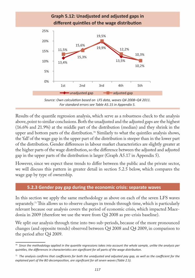
117

Graph 5.12: Unadjusted and adjusted gaps indifferent quintiles of the wage distribution

11,5%15,6%

19,5%

12,2%10,3%

13,4%15,3%

19,9%

13,5%10,2%

0%

5%

10%

15%

20%

25%

1st 2nd 3rd 4th 5th

unadjusted gap adjusted gap

Source: Own calculation based on LFS data, waves Q4 2008–Q4 2011.For standard errors see Table A5.15 in Appendix 5.

Results of the quantile regression analysis, which serve as a robustness check to the analysis above, point to similar conclusions. Both the unadjusted and the adjusted gaps are the highest (16.6% and 21.9%) at the middle part of the distribution (median) and they shrink in the upper and bottom parts of the distribution.70 Similarly to what the quintiles analysis shows, the ‘fall’ of the wage gap in the upper part of the distribution is steeper than in the lower part of the distribution. Gender differences in labour market characteristics are slightly greater at the higher parts of the wage distribution, so the difference between the adjusted and adjusted gap in the upper parts of the distribution is larger (Graph A5.17 in Appendix 5).

However, since we expect these trends to differ between the public and the private sector, we will discuss this pattern in greater detail in section 5.2.5 below, which compares the wage gap by type of ownership.

5.2.3 Gender pay gap during the economic crisis: separate waves

In this section we apply the same methodology as above on each of the seven LFS waves separately.71 This allows us to observe changes in trends through time, which is particularly relevant because our analysis covers the period of economic crisis, which impacted Mace-donia in 2009 (therefore we use the wave from Q4 2008 as pre-crisis baseline).

We split our analysis through time into two sub-periods, because of the more pronounced changes (and opposite trends) observed between Q4 2008 and Q4 2009, in comparison to the period after Q4 2009.

70 Since the methodology applied in the quantile regressions takes into account the whole sample, unlike the analysis per quintiles, the differences in characteristics are significant for all parts of the wage distribution.

71 The analysis confirms that coefficients for both the unadjusted and adjusted pay gap, as well as the coefficient for the explained part of the BO decomposition, are significant for all seven waves (Table 2.5).

118

Graph 5.13: Trends of male and female log hourly wages (left panel) and BOdecomposition components (right panel) between Q4 2008 and Q4 2011

4,194,23 4,24

4,294,25 4,27

3,90

4,04

4,164,12 4,14 4,12 4,14

3,70

3,80

3,90

4,00

4,10

4,20

4,30

4,40

IV 2008 II 2009 IV 2009 II 2010 IV 2010 II 2011 IV 2011

Men

4,09

Women

19,2%

15,0%

6,6%

12,3%15,2%

12,8% 13,4%

22,0%19,2%

12,5%

19,7% 18,4%16,7% 16,9%

0,0%

10,0%

20,0%

30,0%

IV 2008 II 2009 IV 2009 II 2010 IV 2010 II 2011 IV 2011

Unadjusted gap Adjusted gap

Source: Own calculation based on LFS data, waves Q4 2008–Q4 2011.

Changes between Q4 2008 and Q4 2009

Between Q4 2008 and Q4 2009 there was a sharp increase in log hourly wages for both men and women. This was a direct consequence of the new law on income tax in Macedo-nia (see Mojsoska-Blaževski, 2011 for details). This law (introduced to deal with the effects of the crisis) had a stronger impact on female wages than on male: female wages grew by approximately 25.8%, while male wages grew by 13.3% (Graph 5.13, left panel and Table A5.18 in Appendix 5). This may have a been a direct reflection of the fact that women have lower wages, therefore reforms towards more progressive taxation benefited them more than men. This change led to a sharp decrease of the unadjusted pay gap between Q4 2008 and Q4 2009, by 12.6 percentage points (from 19.2% to 6.6%, Graph 5.13, right panel and Table A5.18 in Appendix 5).

However, since there was a change in the LFS question on wages between 2008 and 2009 (instead of being asked the exact wage amounts, individuals were asked to select a wage bracket they belong to), wage data between 2008 and 2009 may not be fully comparable. We would expect this switch from exact reporting of wages to wage brackets to reduce the previous underreporting of wages for both genders and hence induce wage increases, which are not the result of labour market dynamics, but rather of methodological changes. Yet, there is no reason to believe that this would impact reported wages among women dif-ferently than it would impact wages among men. Therefore, it may only be that the entire magnitude of this increase should not be assigned entirely to the change in tax legislation.

During the same period, a decrease in the adjusted pay gap was less pronounced – it dropped by 9.5 percentage points (from 22% in Q4 2008 to 12.5% in Q4 2009).72 The coefficient for the explained part of the BO decomposition dropped from -2.7pp to -5.8pp, meaning that female labour market characteristics improved even further in comparison to male during the analysed period. Thus, the underestimation of the true wage gap in 2009 was even greater than in 2008.

72 The trend was similar between Q2 and Q4 2009, when there were no methodological discrepancies between the datasets.

119

The most important change in labour market characteristics which occurred in this short time span was the increase of female share in high wage jobs, at the tertiary level of edu-cation (by 6 percentage points for women vs. 3 percentage points for men) and among Professionals (by 4 percentage points vs. 1 percentage point for men), while there was a decrease in the share of women among Plant and machine operators (by 6 percentage points vs. 1 percentage points for men). This could have occurred due to the inter-sectoral reshuffling and churning of female and male employees across types of employment during the economic crisis (as we discuss in section 5.1). All the changes observed during this period can be found in Table A5.19 in Appendix 5.

In other words, out of the overall decrease in the unadjusted pay gap (by 12.6 percentage points between Q4 2008 and Q4 2009):

1) the relative improvement of female (compared to male) labour market characteristics (educational level, occupation etc.) accounted for 3.1 percentage points (approxi-mately one fourth of the total decrease);

2) real changes in the distribution of wages for men and women accounted for 9.5 percentage points (approximately three quarters of the total decrease).

Changes between Q4 2009 and Q4 2011

However, the above-observed decrease in the gender wage gap was a one-off effect, since both the unadjusted and adjusted pay gap returned to a higher level, albeit lower than the pre-crisis level, during the following period of analysis.

In Q2 2010, the unadjusted wage gap grew to 12.3% (by 5.7 percentage points), due to the increase in average wages for men (by 1.4%), and a decrease in average wages for women (by 4.2%). The adjusted gap grew even faster than the unadjusted one, to 19.7% (by 7.2 per-centage points). The adjusted pay gap grew faster since female labour market characteristics further improved compared to male, i.e. the explained part of the BO decomposition grew to 7.4pp (by 1.6 percentage points), probably due to labour force churning between types of employment during the crisis. It could have been the case that more men than women with the lowest skill levels entered into employment out of economic necessity due to the negative impact of the crisis.

Since Q2 2010, until the last analysed quarter (Q4 2011), the unadjusted gap slightly increased to 13.4% (by 1.1 percentage points), while the adjusted gap decreased to 16.9% (by 2.8 percentage points), due to a considerable drop in the female advantage in labour market characteristics. Namely, the coefficient for the explained part of the BO decompo-sition fell to 3.5pp (by 4.1 percentage points), mainly due to increase in participation of men with tertiary education, and a decrease of participation of women among technicians (by 4 percentage points).

In general, there seems to have been a lot of churning of labour from certain types of em-ployment into another (e.g. from wage into self-employment), as well as industry-specific changes in the wage structure, which could have depended on the varying extents of GDP contractions that different sectors experienced during the economic crisis.

120

5.2.4 Heckman selection model

The basic idea of the Heckman selection model is to account for the effects of self-selection, i.e. a person’s decision not to work, on the pay gap (assuming that not being in employ-ment is at one’s will). Since a large number of those out of employment in Macedonia are not “willingly out of work,” but unemployed (unemployment rate is above 30% for both men and women), we follow the aproach in Beblo et al. (2003) and eliminate those who are unemployed from the sample of non-employed, and keep only the inactive ones. We further follow Beblo et al. (2003) in dropping those who are (i) younger than 22 and older than 54 (because the selection effects cannot apply for them; and since our robustness analysis suggest that the results in the 15-64 subsample are not robust);73 (ii) inactive and have children under 1 year of age (i.e. parents of newborns). The aim of these restrictions is to have a homogeneous sample of those who are “voluntarily” inactive.

Results of the Heckman estimation procedure show that self-selection is a statistically significant factor for men, but not for women. Namely, invers Mills lambda for men is negative and statistically significant, while for women it is positive, although not statis-tically significant. The signs of the coefficients in the selection equation show that the probability of being employed is (Table A5.20 in Appendix 5):

(i) higher for those with higher level of education,

(ii) lower for men with children aged 3-6 years old; lower for women with children of any age,

(iii) higher for those who have partners and whose partners work,

(iv) higher for younger and older working age population members.

In the interpretation of selection effects we follow the approach from Neuman and Oaxaca, (2004) named “decomposition of the selectivity corrected wage differential.” This aproach represents the decomposition of the selection-adjusted wages.74 Table 5.14 summarises the analysis of selection effects on the gender pay gap.

Column “without selection” shows the results of the BO decomposition without applying Heckman’s selection procedure. The unadjusted gap for the 22-54 sample is slightly higher than for the 15-64 sample and it stands at 14.8%. The effects of the characteristics point to the fact that the gap is “underestimated” due to better female labour market characteristics (by 4pp) and that the adjusted gap is 18.8%.

73 Namely, the results from two estimation procedures for the 15-64 sample (Heckman’s two-step procedure and maximum likelihood procedure) point to different conclusions (Table A5.20 in Appendix 5), while for the subsample 25-54 subsample the results point to the same conclusion (Table A5.20 in Appendix 5). In results we show the results from the maximum likelihood procedure.

74 The interpretation of the selection effect in BO decomposition is still a matter of debate. Neuman and Oaxaca (2004) further suggest there are “alternative decompositions that could be considered but that require stronger assumptions and perhaps value judgements about what constitutes inequity.”

121

Table 5.14: Blinder-Oaxaca decomposition with and without selection correction

Without selectioncorrection

With selection correction

Men (average log hourly wage) 4.214*** 4.243***

(0.005) (0.008)

Women (average log hourly wage) 4.065*** 4.055***

(0.006) (0.018)

Difference (unadjusted gender pay gap) 0.148*** 0.188***

(0.007) (0.020)

Explained part -0.040*** -0.040***

(0.005) (0.005)

Unexplained part (adjusted pay gap) 0.188*** 0.227***

(0.006) (0.019)Source: Own calculation based on LFS data, waves Q4 2008–Q4 2011.

Robust standard errors in parentheses. Notes: * p<.1; ** p<.05; *** p<.01

Since men with low predicted probability of participation are predicted to earn less than men with similar productivity endowment (i.e. labour market characteristics) but with a higher predicted probability of participation, their wages should be corrected upward. Thus, the corrected wages for men are higher (for almost 3%) in the “with selection” column, than in the “without selection” column (Table 5.14).

On the other hand, since the positive (although statistically insignficant) Lambda (Table A5.20) for women suggests that women with lower predicted probability of participation are predicted to earn more than women with similar productivity endowment (i.e. labour market characteristics) but with a higher predicted probability of participation, their wages should be corrected downward. Thus, the corrected wages for women are lower (for 1%) in the “with selection” column, than in the “without selection” column (Table 5.14).

The corrected wages differential, therefore, is higher than the “uncorrected,” leading to the increase of the wage gap. The explained part of the BO decomposition stays at the same level, but the unexplained is corrected upwards by 4%, since the effect of the selection is in the unexplained part of the equation (Table 2.7). In total, the adjusted gap increases to 22.7% when selection is taken into account.

122

5.2.5 Gender pay gap across type of ownership: private vs. public sector analysis

In this section we compare the gender pay gap between the private and public sectors in Macedonia.75 Due to strong labour market duality in the Western Balkans, where the public and the private sector operate under different “rules of the game,” this analysis can provide important policy insights.

Table 5.15 shows that in both sectors all indicators for the BO decomposition (the un-adjusted pay gap, the explained part and the adjusted pay gap) are statistically significant.

Table 5.15: Blinder-Oaxaca decomposition: for public and private sector separately

Public Private Difference

Men (log hourly wage) 4.434*** 4.108*** 32.6%

(0.007) (0.005)

Women (log hourly wage) 4.394*** 3.931*** 46.3%

(0.008) (0.006)

Difference (unadjusted pay gap) 0.040*** 0.177*** -13.7pp

(0.011) (0.008)

Explained part -0.074*** -0.008* -6.6pp

(0.008) (0.005)

Unexplained part (adjusted pay gap) 0.114*** 0.185*** -7.1pp

(0.009) (0.007)

Sample size 6,801 12,937Source: Own calculation based on LFS data, waves Q4 2008–Q4 2011.

Notes: Robust standard errors in parentheses. * p<.1; ** p<.05; *** p<.01† A detailed BO decomposition for public/private sector is available in Appendix 5 (Table A5.25).

On average, for both women and men, wages are higher in the public than in the private sector. This difference is higher for women, since their average wage in the private sector is by 46.3% lower than their average wage in the public sector. This difference for men stands at 32.6% (Table 5.15 and Graph 5.16, left panel).

Consequently, the unadjusted wage gap is substantially higher in the private than in the public sector – by 13.7 percentage points. While in the private sector men receive 17.7% higher wages than women on average, this difference in the public sector is “only” 4% (Table 5.15 and Graph 5.16, right panel).75 However, we are concerned that the sector of ownership is endogenous to the type of occupation (e.g. for teachers, doctors) as well as to the level of education (because there is a higher portion of educated individuals working in the public sector by default).

123

Graph 5.16: Male and female log hourly wages (left panel) and wage gaps (right panel) in the private and public sectors in Macedonia

4,43

4,11

4,39

3,93

3,6

3,8

4,0

4,2

4,4

4,6

Public Private

Wages

Men Women

4,0%

17,7%

11,4%

18,5%

0,0%

5,0%

10,0%

15,0%

20,0%

Public Private

Wage gap

Unadjusted gap Adjusted gap

Source: Own calculation based on the LFS data, waves Q4 2008–Q4 2011.

However, once we adjust the wage gap to account for different labour market charac-teristics between men and women in the two sectors, the gap widens significantly in the public sector – from 4 to 11.4%, while it grows only slightly in the private sector – from 17.7 to 18.5% (Table 5.15 and Graph 5.16, right panel). This is because women in the public sector have significantly better labour market characteristics than men, while this difference in the private sector is very low and is not statistically significant. This can also be considered a type of discrimination, since women need to be better educated than men to access the same positions in the public sector.

Differences in characteristics in the private vs. the public sector

Graph 5.16 shows the most important labour market characteristics that underestimate the gender pay gap in the public and the private sector. In the public sector, the most important ones are the effects of education and occupation. Better female positioning regarding these two characteristics underestimates the gap by 3.7pp and 4pp respectively.

On the other hand, in the private sector, labour market characteristics of individuals do not underestimate the gap significantly, so none of the characteristics have an impact on the wage gap higher than 1 percentage point (either negative or positive, Graph 5.17). How-ever, a detailed analysis of labour market characteristics that underestimate or overestimate the gap in the private sector reveals certain differences that cancel each other out (Table A5.23 in Appendix 5).

124

Graph 5.17: Detailed Blinder-Oaxaca decomposition by sector of ownership – explained part – the impact of differences in characteristics between

the genders on the gender wage gap (in percentage points)

-5 -4 -3 -2 -1 0 1 2

Educa�on

Tenure

Occupa�on

Sector of ac�vity

Type of contract

Gender wage gap

Private Public

Source: Own calculation based on LFS data, waves Q4 2008–Q4 2011.For standard errors see Table 5.23 in the Appendix5.

Table 5.18 shows in detail the explained part of the unadjusted gap in the public sector. The most important positive characteristic of women is their higher share in high wage jobs, which require tertiary education (by 14 percentage points: 49.6% of women, 35.1% of men) and a higher share of women among Professionals (by 10.7 pp: 33.9% of women; 23.2% of men) (Table A5.25 in Appendix 5). Additional better characteristics of women include their higher frequency (in comparison to men) in high pay jobs of Technicians and in Modern Services, and their lower frequency in low pay jobs: Primary and secondary education, Craft and trades workers, Plant and machine operators and Service and sales workers, as well as in Agriculture (Table A5.25 in Appendix 5).

On the other hand, their worse labour market characteristics, which make the unadjusted pay gap in the public sector overestimated, are lower frequency of women in high pay jobs such as Senior officials and managers and in Public services, as well as their higher frequency in Traditional services (Table A5.25 in Appendix 5). If these characteristics were the same the unadjusted gap in the public sector would be lower (Table 5.18).

In total, better characteristics of women in comparison to men in the public sector prevail over the worse ones, so that the overall unadjusted gap is underestimated, i.e. it would be higher (by 7.4pp) if women were to have the same characteristics as men.

In the private sector, better and worse female characteristics in comparison to men cancel each other out, so that overall, the explained part of the gap is only marginally significant. In other words, if women were to have the same characteristics in the labour market as men, the increase of the unadjusted wage gap would be only marginally significant.

The most important better characteristic of women in the private sector is their lower frequency among Craft workers (by 21 percentage points: 5% of women, 26.5% of men, Table A5.25 in Appendix 5), which underestimates the gap by 2%. Additionally, a better

125

characteristic of women is their higher frequency in high pay jobs: those which require ter-tiary education, among Professionals, Technicians and associate professionals and Clerks and in Modern and Public Services; and their lower frequency in low pay jobs: those which require primary education only, among Elementary occupations and in Agriculture (Table 5.19).

Table 5.18: Detailed Blinder-Oaxaca decomposition in the public sector –explained part – detailed impact of differences in characteristics

between the genders on the gender wage gap

High wage jobs Low wage jobs

Higher frequency of women

Tertiary education (-2.7pp)Tenure (-0.2pp)

Professionals (-2pp), technicians and associate

professionals (-0.6pp), Modern(a) services (-0.1pp)

These characteristics make the true gap seem smaller.

Traditional services(c) (0.3pp)

These characteristics make the true gap seem larger.

Lower frequency of women

Managers (0.7pp)Public Services(b) sector (0.5pp)

These characteristics make the true gap seem larger.

Primary and secondary education (-1pp)

Craft and trades workers (-1.2pp), Plant and machine

operators (-0.5pp) and Service and sales workers (-0.4pp)

Agriculture (-0.3pp)

These characteristics make the true gap seem smaller.

Source: Own calculation based on LFS data, waves Q4 2008–Q4 2011. For standard errors see table 5.25 in Appendix 5.

Note: Numbers in brackets show how much the gap is underestimated or overestimated when not adjusted for the difference in the characteristic. Percentage points shown in brackets show contribution of each char-

acteristic to the adjustment of the total gap.Footnotes: (a) Communication, Financial intermediation, Real estate, Experts (b) Public administration,

Education, Health, Social service activities, ET organisations (c) Trade, HORECA, Transport

The most important worse labour market characteristic of women in the private sector is their higher frequency among Plant and machine operators (by 13.4 percentage points: 31.6% women vs. 18.2% men) and Service and sales workers (by 7.6 percentage points:

126

24.4% women vs. 16.8% men). Additionally, women have a low frequency in high pay jobs among Senior officials and managers and in jobs which are characterised by higher tenure (Table 5.19 and Table A5.25 in Appendix 5).

Table 5.19: Detailed Blinder-Oaxaca decomposition in the private sector – explained part – detailed impact of differences in characteristics

between the genders on the gender wage gap

High wage jobs Low wage jobs

Higher frequency of women

Tertiary education (-0.5pp)Professionals (-0.2pp), technicians

and associate professionals (-0.1pp), Clerks (-0.1pp)

Modern(a) (-0.2pp) and Public(b) services (-0.2pp) sector

These characteristics make the true gap seem smaller.

Service and sales workers (1.5pp), Plant and machine operators (2.5pp)

These characteristics make the true gap seem smaller.

Lower frequency of women

Higher tenure (0.5pp)Managers (0.2pp)

These characteristics make the true gap seem smaller.

Primary education (-0.5pp)Craft and trades workers (-2pp), Elementary occupations (-0.8pp)

Agriculture (-0.5pp)

These characteristics make the true gap seem smaller.

Source: Own calculation based on LFS data, waves Q4 2008–Q4 2011. For standard errors see table 5.25 in Appendix 5.

Note: Numbers in brackets show how much the gap is underestimated or overestimated when not adjusted for the difference in the characteristic. Percentage points shown in brackets show contribution of each char-

acteristic to adjustment of the total gap.Footnotes: (a) Communication, Financial intermediation, Real estate, Experts (b) Public administration,

education, Health, Social service activities, ET organisations

Differences in returns to labour market characteristics in the private vs. the public sector

The largest part of the adjusted gender wage gap in both the public and the private sec-tor exists due to unobservable characteristics between men and women, which account for 92% of the adjusted pay gap in the public (10.6 of 11.4%) and 80% in the private sector (14.7 of 18.5%) (Graph 5.19 and Graph 5.21).

127

The rest of the unexplained gap (8% in the public and 20% in the private) occurs because of different returns to observable personal characteristics of labour market partici-pants. A detailed disaggregation of the unexplained part of the adjusted wage gap shows significant differences in returns between the public and the private sector. While in the private sector there are no differences in returns to education, in the public sector, women have lower returns to secondary and tertiary education, by 2.4 percentage points in total (1.4pp to secondary, 1.5pp to tertiary). However, in the public sector women have higher returns to occupational characteristics (by 6.1pp), while in the private sector their returns to occupational characteristics are lower than male (by 4pp). While in the private sector the differences in returns to the sector of activity are only marginally significant, in the public sector women have significantly lower returns (Graph 5.20 below and Table A5.24 in Appendix 5).

Graph 5.20: Detailed Blinder-Oaxaca decomposition by sector of ownership – unexplained part – the impact of differences in returns to characteristics

and differences in unobservable characteristics between the genders on the gender wage gap (in percentage points)

-10 -5 0 5 10 15 20

Educa�on

Tenure

Occupa�on

Sector of ac�vity

Type of contract

Unobservablecharacteris�cs

Gender wage gap

Private Public

Source: Own calculation based on LFS data, waves Q4 2008–Q4 2011.

In the public sector, overall differences in returns (to education, occupation and activity) account for a very small part of the unexplained part – 8%, since they work in the opposite direction and therefore cancel each other out (Graph 5.20 and Table A5.24 in Appendix 4). Furthermore, the observed differences in returns to education and sector of activity could most likely represent a statistical artefact due to the usage of inter-correlated independent

128

variables. In other words, in the public sector, wage returns to a job conducted by a person with the same education, within the same occupation and in the same sector of activity do not differ significantly for men and women, i.e. they are only slightly higher for men, by 0.8%.

On the other hand, in the private sector, the difference in returns accounts for a larger part of the unexplained gap (around 20%, i.e. 3.8% out of 18.5%). A detailed analysis reveals that the main differences in returns exist among Plant and machine operators, where women have 4.4pp lower returns when entering this occupation. This may either be due to the fact that employers actively discriminate against women by valuing their labour market skills as less worthy than male, or because employers in the private sector value certain personal characteristics of workers which we cannot observe but which systematically differ between the genders. These could vary from differences in female and male labour market behaviour which employers reward/punish, e.g. that women may be less flexible in terms of working hours or business trips due to reproductive/home responsibilities, to other immeasurable effort- and ability-related variables, as well as to labour market frictions.

Graph 5.21: Detailed Blinder-Oaxaca decomposition – structure of the unexplained part

11.4%

18.5%

0,0%

5,0%

10,0%

15,0%

20,0%

Public Private

Structure of adjusted gap

Differences in unobservable characteris�csDifferences in returns

Source: Own calculation based on LFS data, waves Q4 2008–Q4 2011.

Differences at different points of the wage distributionin the private vs. the public sector

In this section we analyse the wage gap at the different points of the wage distribution of in the public and private sectors separately. We split the sample into five wage brackets (quin-tiles) and compare differences in wages between men and women within wage quintiles.76 76 We drop the dummy variables for year effects in the BO decomposition analysis. Our preliminary analysis showed a significant impact of time effects on the explained part of the gap, which is impossible to interpret, due to difference in the

129

In the public sector, the unadjusted gap is the lowest within the first three quintiles of the wage distribution (1st to 3rd). The gap in those quintiles is not statistically significant and within the 2nd quintile it is even in favour of women. At the higher parts of the wage distribution in the public sector, the unadjusted wage gap is significantly higher, reaching its maximum of 7.1% within the 5th quintile (the top 20% of all wages in the public sector; Graph 5.22 and Table A5.26 in Appendix 5). The adjusted gap follows the trend of the unadjusted: the adjusted gap is low within first three quintiles of the distribution and it increases within the 4th and the 5th quintiles. Therefore, there is a clear glass ceiling effect in the public sector, meaning that women cannot access the best-paid jobs to the same extent as men.

The differences between the first three and the last two quintiles in the adjusted gap are slightly lower since the female characteristics in the first three deciles are better than male, so they lower the gap by 1.7, 1.9 and 1.2pp within the 1st, 2nd and 3rd quintile. On the other hand, in the last two quintiles (4th and 5th) the differences in characteristics (explained part) are statistically insignificant (Table A5.26 in Appendix 5).

Most importantly, the better female position within the first three quintiles of the wage distribution is due to their better occupational structure, mainly, their lower frequency among Plant and machine operators and their higher frequency among Technicians (in the 2nd

quintile) and professionals (in the 3rd quintile). Additionally, within the 1st quintile, the better female position is due to their lower frequency in the low paid Industry sector. Within the 2nd quintile, the better female position is due to higher frequency of women with tertiary education and lower of those with primary education, while within the 3rd quintile, it is due to the higher female frequency in the Public services sector (Table A5.28 in Appendix 5).

Graph 5.22: Unadjusted and adjusted pay gap at different pointsin wage distribution for public (left panel) and private sector (right panel)

0,9%- 0,9%

1,0%

7,3%2,6%

1,0%2,2%

6,4%7,1%

-2%

0%

2%

4%

6%

8%

1st 3rd 4th 5th

Public sector

6,1%

2nd

unadjusted gap adjusted gap

14,8%

16,4%17,9%

23,1%

17,8%

17,4%

16,2%17,5%

23,6%

19,4%

10%

15%

20%

25%

1st 2nd 3rd 4th 5th

Private sector

unadjusted gap adjusted gap

Source: Own calculation based on LFS data, waves Q4 2008–Q4 2011. For standard errors see tables 5.26 and 5.27 in Appendix 5

definition of the wage variable through years. Namely, interpretation of this coefficient would go to compare participation of men and women in survey waves and interpret the differences as higher participation in years where the wages were higher. As already discussed in section 5.2.3 our analysis, there are some methodological issues with comparisons of wage levels across years, so the impact of this variable on the explained part cannot be interpreted.

130

In the private sector the unadjusted gap is the lowest within the 1st quintile of the wage distribution (14.8%) and it rises until the 4th quintile, where it reaches its peak (23.1%). It then drops to 17.8% within the 5th quintile (the highest 20% of all wages in private sector)

In all the quintiles of the wage distribution in the private sector, differences in characteris-tics are in favour of women, but they are statistically significant only at the top and bottom of the wage distribution (Table A5.27 in Appendix 5). They adjust the wage gap within the 1st and 5th quintile by 2.7pp and 1.6pp respectively. Therefore, the glass ceiling is a lot more pronounced in the private sector, where women cannot access the top paid positions to the same extent as men with the same labour market characteristics.

The most important characteristic at the top part of the distribution is better education of women and their higher frequency in Modern services. The female advantage within the 1st quintile is mainly caused by the fact that women more often have written contracts, as well as by lower female frequency in the lower paid Industry sector and among the low wage Plant and machine operators (Table A5.29 in Appendix 5). This is rather intuitive, as female labour supply is more wage elastic than male (because they chose between re-productive/house work, leisure and paid work, while men choose between leisure and paid work only), so women are more likely to select away from employment when wages are too low. Furthermore, women are more concerned with quality of employment, so as second earners in the household, they can “afford” to self-select away from precarious employment without written contracts (see literature review in Chapter 2 for details).

5.3 Gender pay gap among the self-employed

In this section, we focus on the gender pay gap among the self-employed in Macedonia. This group of workers consists of two distinct sub-groups: the self-employed persons and owners of businesses. For both of these groups, data on earnings are available. The number of self-employed women in Macedonia is significantly lower than men. Women make 24% of all business owners and 15.4% of all self-employed.

The sample used for estimating the Mincerian wage regression and the Blinder-Oaxaca decomposition includes 4,627 persons (3,787 men and 840 women) from seven waves of the Macedonian Labour Force Survey (LFS), covering the period between Q4 2008 and Q4 2011. The sample includes all workers in self-employment77 between 15-64 years of age who receive positive earnings.78 Our dependent variable is log hourly real wage.79

Table 5.23 shows estimation results of the four different specifications (S1 to S4) of the Mincer wage regression (along the lines of our analysis for wage employment). The

77 This analysis excludes unpaid contributing family members. We also exclude part-time workers and workers who are in education or training.

78 65 cases with zero wages are excluded from the analysis.

79 Wages in the 4th quarter of 2008 are reported as exact wage amounts, while in the consecutive waves respondents select a wage bracket for their earnings. In 2009 and 2010 there were 10, and in 2011 there were 11 wage brackets. Wages are transformed from nominal to real wages using the Consumer Price Index (CPI) with the 4th quarter of 2008 as baseline. The data on CPI were taken directly from Macedonian Statistical Office (Drzaven Zavod za Statistika) website.

131

coefficient for gender in specification S1, where female is the only independent variable, represents the unadjusted gender pay gap. Coefficients in specifications S2-S4 represent the pay gap adjusted for variables marked with x. Coefficients for all explanatory variables in the Mincer equation are reported in Table A5.30 in Appendix 5.

Table 5.23: Mincer wage regressions for self employed (Specifications S1 to S4)

Variable S1 S2 S3 S4

Female -0.070*** -0.159*** -0.159*** -0.186***

(0.023) (0.022) (0.022) (0.021)

Education and tenure Yes Yes Yes

Time fixed effects Yes Yes

Work related variables (1) Yes

Sample 4,627 4,627 4,627 4,627

Adjusted R-square 0.002 0.118 0.131 0.240

Log Likelihood -4093 -3808 -3773 -3463

Source: Own calculation based on LFS data, waves Q4 2008–Q4 2011.Robust standard errors in parentheses. Notes: * p<.1; ** p<.05; *** p<.01

(1) Occupation (ISCO), Sector of activity (NACE), Self-employment status (owner/entrepreneur).

Column S1 in Table 5.23 shows that self-employed women in Macedonia, on average, have 7% lower hourly earnings than men. The gap widens to 15.9% when adjusted for education and tenure (specification S2). Coefficients for the two education dummy variables are positive and rising with the higher level of education. Coefficients for the two education dummy variables measuring secondary and tertiary education are positive and rising with level of education (elementary education is the omitted category), showing that returns to education increase with education, such that those with secondary and tertiary education have 16.4% and 56%, respectively, higher wages than individuals with elementary education only. The coefficient for tenure is insignificant, and adding time fixed effects (specification S3) does not change the coefficient for gender (nor for education and tenure), suggesting that the specification is robust.

The wage gap additionally increases to 18.6%, when additional job characteristics are taken into account (specification S4). The results show the expected impact of job char-acteristics on earnings from self-employment. Earnings are: (i) higher for professionals, managers and technicians, than for all other occupations and lower for occupations such as Service and sales workers, Craft and trades workers, Plant and machine operators and Elementary occupations; (ii) are higher in Modern services (Communication, Financial intermediation, Real estate, Experts) than in all the other sectors; (iii) higher among own-ers than self-employed (without employees). Coefficients for education stay positive and rising with the level of education, but returns to education are substantially lower due to

132

correlation with job characteristics, with the coefficient for secondary education losing its statistical significance (Table A5.30 in Appendix 5).

Table 5.24 shows that in self-employment as well as in wage employment, analysed earlier, all indicators for the BO decomposition (the unadjusted pay gap, the explained part and the adjusted pay gap) are statistically significant.

Table 5.24 Blinder-Oaxaca decomposition in employment and self-employment(a)

EmploymentSelf-

employmentDifference

Men (log hourly wage) 4.222*** 3.904*** 31.8%

(0.004) (0.009)

Women (log hourly wage) 4.088*** 3.834*** 25.4%

(0.005) (0.021)

Difference (unadjusted pay gap) 0.134*** 0.070*** 6.4pp

(0.007) (0.023)

Explained part -0.045*** -0.116*** 7.1pp

(0.005) (0.013)

Unexplained part (adjusted pay gap) 0.179*** 0.186*** -0.7pp

(0.006) (0.021)

Sample 19,738 4,627SSource: Own calculation based on LFS data, waves Q4 2008–Q4 2011.

Notes: Robust standard errors in parentheses. * p<.1; ** p<.05; *** p<.01(a) Full table for BO decomposition for is available in Appendix 5 (wage-employment Table A5.13; self-

employment Table A5.31).

The unadjusted gap in self-employment is 7%, which is considerably lower than the respec-tive gap in wage employment (by 6.4 percentage points, Graph 5.25, right panel). It should be noted that wages in wage employment are significantly higher than in self-employment (by 31.8% for men, and 25.4% for women, Graph 5.25, right panel).

Similarly to wage employment, women in self-employment have better labour market characteristics than men, which “underestimates” the gap by 11.6%. In other words, if women and men were to have the same characteristics in self-employment the differ-ence in wages would be significantly higher – 18.6%. Thus the adjusted gap is slightly higher in self-employment than in employment (by 0.7pp)80, since the difference in labour market characteristics in self-employment is higher than in employment.

80 This difference is not statistically significant, since the 95% confidence intervals overlap.

133

Graph 5.25: Male and female log hourly wages (left panel) and wage gaps (right panel) in self-employment and employment in Macedonia

4,22

3,90

4,09

3,83

3,6

3,8

4,0

4,2

4,4

Wage-employment Self-employment

Wages

Men Women

13,4%

7,0%

17,9% 18,6%

0,0%

5,0%

10,0%

15,0%

20,0%

Wage-employment Self-employment

Wage gap

Unadjusted gap Adjusted gap

Source: Own calculation based on LFS data, waves Q4 2008–Q4 2011.

Differences in characteristics among the self-employed

Graph 5.26 (blue bars) shows that the most important labour market characteristics which underestimate the true pay gap in self-employment are education, occupation and status in self-employment (self-employed vs. business owner). Better female positioning regarding these three characteristics underestimates the gap by 1.8%, 6.9% and 2.4% respectively.

Graph 5.26: Blinder-Oaxaca decomposition –differences in characteristics and returns(a)

-10 -5 0 5 10 15 20

Educa�on

Tenure

Occupa�on

Sector of ac�vity

Status(self-employed/owner)

Unobservablecharacteris�cs

Gender wage gap

Differences in returns Differences in characteris�cs

Source: Own calculation based on LFS data, waves Q4 2008–Q4 2011.(a) Tables for BO decomposition are available in Appendix 5 (Table A5.31 and A5.32).

Table 5.27 shows the detailed analysis of the explained part of the unadjusted gap in self-employment. Educational differences underestimate the gap since women with tertiary

134

education can more frequently be found among the self-employed and women with primary education less frequently (probably, as we discuss earlier, because low skill men who work in family farms tend to report as self-employed while their wives as contributing family members), (Table A5.32 in Appendix 5). Among occupations, a higher share of women among Managers and Professionals and their lower frequency in jobs such as Service and sales workers and Elementary occupations (Table A5.32 in Appendix 5), lowers the gap by 1.3%, 1% and 3.5%, respectfully. Finally, a higher share of women among business owners (Table A5.32 in Appendix 5) underestimates the gap by 2% (Table 5.27).

Table 5.27: Detailed Blinder-Oaxaca decomposition – explained part – self-employed

High wage jobs Low wage jobs

Higher frequency of women

Tertiary education (-1.1%)Managers (-1%), Profes-

sionals (-1.5%)Owner (-2.4%)

These characteristics make the true gap seem smaller.

Lower frequency of women

Primary education (-1.2%)Service and sales workers (-0.3%)

and Elementary occupations (-4.8%)

These characteristics make the true gap seem smaller.

Source: Own calculation based on LFS data, waves Q4 2008–Q4 2011.Notes: Percentage points shown in brackets show contribution of each characteristic to adjustment of the

total gap in the public sector.

On the other hand, since none of the differences in returns are statistically significant, most of the unexplained part of the gap is due to differences in unobservable characteristics between the genders (16.7% out of 18.5%), (Graph 5.26, red bars and Table A5.31 in Ap-pendix 5, Unexplained part). This may be linked to the fact that men have more access to initial capital for investment and stronger informal networks, which may positively affect their returns.

135

6. Gender Pay Gap in Montenegro

6.1 Labour market trends in Montenegro

6.1.1 Main labour market indicators

Female employment rate in Montenegro is significantly lower than male. Gender gap in employment rates stood at an average of -13.4 percentage points during the analysed period (Q4 2008-Q4 2011). The observed gender gap in employment is mainly caused by higher inactivity of women, which is on average by 15.2 percentage points above men’s. Unemployment is also higher among women than among men, but to a far lesser extent – gender unemployment gap stood at an average of 1.8 percentage points during the period of analysis (Graph 6.1).

Graph 6.1: Main labour market indicators, Q4 2008 – Q4 2011

5954,9 54,6

49,5

30

40

50

60

70

Q4

2008

Q4

2009

Q4

2010

Q4

2011

Employment rate (%)

Male Female

15,1

19,3 19,1 18,7

10

20

30

Q4

2008

Q4

2009

Q4

2010

Q4

2011

Unemployment rate (%)

Male Female

30,1 32 32,539,1

20

30

40

50

60

Q4

2008

Q4

2009

Q4

2010

Q4

2011

Inac�vity rate (%)

Male Female

Source: MONSTAT LFS reports, for population 15-64.

Between Q4 2008 and Q4 2011, all the main labour market indicators worsened for work-ing age men, while they mostly stayed stable for working age women. However, worsening of the male position in the labour market led to reductions in gender gaps in labour market indicators. While male employment rate remained at around 42%, the employment gap was reduced by 9.2 percentage points (from -17 to -7.8 percentage points).

During the same period, male unemployment rate rose by 3.6 percentage points (from 15.1% to 18.7%), while female unemployment rate oscillated, reaching its peak of 21.9% in Q4 2009, only to drop to 17.7% in Q4 2011 (by 0.6pp lower than in Q4 2008). Thus, while female unemployment rate was higher than male by 3.2pp in Q4 2008, male unemploy-ment rate surpassed the female one in Q4 2011 by 1pp (17.7% for women vs. 18.7% for men).

Although the level of female inactivity is significantly higher than male, rise of inactivity during the observed period was a lot more pronounced for men than for women. While female inactivity remained relatively stable (it rose by 1.1pp), male inactivity rose by 9pp (from 30.1 to 39.1%). Therefore the gender gap in inactivity shrank by 7.9 percentage points over the analysed period (from 18.1 to 10.2).

136

The worsening of all labour market indicators for men in Montenegro indicates that men were more impacted by the crisis than women. This could be due to the fact that women can more frequently be found working in the public sector, which was better insulated from the crisis than the private sector. Furthermore, the fact that women who work are on average better educated and more skilled than men who work may have contributed to this trend, because low-skilled workers are more likely to lose jobs during the crisis than high-skilled ones. Finally, most of the job losses during the crisis occurred in the industry sector, which traditionally employs a more male workforce. The peculiar fact that male inactivity rose three times as much as male unemployment may indicate the unavailability of new jobs and discouragement from seeking new employment for those who have lost their jobs during the economic crisis.

Graph 6.2: Employment rate by… ... gender and level of education (15-64) … gender and age (15-64)

27%

56%

76%

12%

43%

76%

Primary Secondary Terary

Male Female

17%

69%

47%

13%

55%

25%

15-24 25-54 55-64

Male Female

Source: Own calculation based on the LFS data, waves Q4 2008–Q4 2011

The gender employment gap is the highest at the level of primary (15.4 percentage points) and secondary (13.1 percentage points) education, while it is non-existent at the tertiary level of education (Graph 6.2, left panel).

The gender employment gap is the most pronounced among the oldest members of the labour force (55-64). Their employment gap (22.6 percentage points) is significantly higher than the gap observed among women and men in the prime age group of 25-54 years (14 percentage points) and youth (4.5 percentage points). We can probably explain this by the changing role of women, as well as the fact that younger women are more educated than those from older generations. The low gender employment gap among youth may also be due to the very low baseline, i.e. very low levels of youth employment more generally (Graph 6.2, right panel).

Finally, for the oldest working age group (55-64) the gap in employment could be caused by the fact that women retire earlier than men in Montenegro81.81 Although in 2010, retirement age equalised for the two genders and increased to 67 years of age, there is a long transi-tion period which still results in many workers of both genders retiring much earlier.

137

6.2 Type of employment

Over the analysed period (Q4 2008–Q4 2011), both men and women in Montenegro can most often be found in wage employment (79% of men and 89% of women; Graph 6.3, left panel). Although a higher percentage of employed women are in wage employment than men, women are a minority in total wage employment (46.1% of the total). The fact that fewer women work overall could imply that women are more likely to choose employment only if it is better quality and lower risk (i.e. wage employment) in comparison to men, who are less wage elastic and will work regardless of the type of work which is available to them. Men are twice as represented among the self-employed (around 20% of men and 10% of women). Percentages of unpaid family members, who most often work in agriculture and elementary occupations, have been extremely low and they are comparable across the two genders (1% of each gender; Graph 6.3, left panel).

Graph 6.3: Structure of employment by type and gender (15-64)…

…and share of womenby type of employment (15-64)

46

28

43

45

26

41

47

38

53

00 10 20 30 40 50 60

Wage-employed

Self-employed

Unpaid family members

Q4 2011 Q4 2008 Average for all wages

89 79 88 77 87 82

10 20 11 22 13 17

01 01 01 01 01 01

0%

10%

20%

30%

40%

50%

60%

70%

80%

90%

100%

Female Male Female Male Female Male

Average for allwaves

Q4 2008 Q4 2011

Unpaid family members Self-employed Wage employed

Source: Own calculation based on the LFS data, in the period Q4 2008 to Q4 2011. Weighted sample.

Over the analysed period, the structure of employment among the two genders stayed more or less stable: while the percentage of self-employed women increased from 10.5% to 12.7%, percentage of self-employed men decreased from 21.7% to 17.2%. On the other hand, percentage of wage-employed women decreased from 88.3% to 86.6%, whereas percentage of wage-employed men increased from 77.1% to 82.4% (Graph 6.3, left panel). However, since overall male employment significantly fell relative to female during the observed period, the share of women among the self-employed and unpaid family mem-bers rose sharply between Q4 2008 and Q4 2011 (from 26 to 38% and from 41 to 53% respectively; Graph 6.3, right panel).

138

Within all educational categories, most men and women are found in wage employment (Table A6.1 in Appendix 6).82 The percentage of wage-employed men and women increases with the level of education, from 60% (primary education) to 85% (tertiary education) for men, and from 58% (primary education) to 94% (tertiary education) for women. At the same time, the percentage of self-employed men and women decreases with the level of education, from 34% (primary education) to 15% (tertiary education) for men, and from 33% (primary education) to 5% (tertiary education) for women. These data seem to indicate that much of the self-employment in Montenegro is last resort, i.e. due to lack of opportunities for wage employment, rather than opportunity based.

The percentage of unpaid or contributing family members decreases with the level of education, from 5% (primary education) to 0.1% (tertiary education) for men, and from 9% (primary education) to 0.1% (tertiary education) for women. At the tertiary level of education (i.e., university degree or higher), percentage of unpaid or contributing family members among both men and women in Montenegro is close to zero.

The overall share of employed women increases with the level of education, from 35% (primary education) to 51% (tertiary education). The share of women in wage employment also increases with the level of education, from 35% (primary education) to 53% (tertiary education), while the share of women in self-employment decreases with the level of education, from 35% (primary education) to 27% (tertiary education). The share of female unpaid family members is close to the share of male unpaid family members across all educational categories.

Observed by age, most men and women are found in wage employment within all age groups (Table A6.2 in Appendix 6). The percentage of wage-employed men and women decreases with age, from 83% (15-24 years) to 81% (55-64 years) for men, and from 91% (15-24 years) to 85% (55-64 years) for women. Among the self-employed, the highest percentage of both men and women is in the age category 25-54 years (20% of men and 10% of women).

The overall share of employed women decreases with age, from 41% (15-24 years) to 36% (55-64 years). The share of wage-employed women starts at 43% for the youngest age group (15-24 years), peaks at 48% for the middle age category (25-54 years), and drops down to 38% for the most senior age category (55-64 years). Although lower than the share of self-employed men at all age categories, the share of self-employed women in Montenegro increases with age, from 22% (15-24 years) to 30% (55-64 years). The share of female unpaid or contributing family members increases with age, from 44% (15-24 years) to 53% (55-64 years), but the percentages of unpaid or contributing family members are quite low in all age categories for both men and women.

The percentage of wage-employed is higher among both men and women in urban areas (83% men and 93% women) than in rural areas (72% men and 78% women) (Table A6.3 in Appendix 6). On the other hand, the percentage of self-employed and unpaid family members is higher among both men and women in rural areas than in urban areas. The latter can be explained by the fact that there are more agricultural workers in rural areas.82 Appendix 6 - appendix to this chapter with supporting data referenced throughout, is available online only, at www.fren.org.rs/node/220.

139

The overall share of employed women is higher in urban (47%) than in rural areas (35%). There is a higher share of female unpaid family members in rural (43%) than in urban areas (41%), which is “compensated,” on the other hand, by a higher share of wage-employed women in urban (50%) than in rural areas (37%).

Analysed by regions (north/central/coastal), the percentage of wage-employed men and women is the lowest in the north (68% of men and 82% of women) and the highest in the central region (84% of men and 93% of women) (Table A6.4 in Appendix 6).The share of women in wage employment increases from the north (41%) to the south (48%).

In all regions, the percentage of self-employed women is lower than the percentage of self-employed men by between 6 (coastal) and 14 percentage points (north). The share of women in self-employment increases from the north (22%) to the south (37%). Unpaid family members are most often found in the north (3% of men and 4% of women), which also has relatively more agricultural workers. However, in all regions the percentages of unpaid or contributing family members among both men and women are very low.

6.1.3 Unadjusted gender wage gap and labour market characteristics

In this section we focus on wage employment only, which is the sub-sample of employees that we use in our regresion analysis. We describe wage characteristics for men and women, gender differences in wages as well as the structure of wage employment.

The sample that we use throughout our analysis consists of 8,969 individuals (4,973 men and 3,996 women) for whom we observe wages in the LFS in the period from the 4th quarter of 2008 to the 4th quarter of 2011 (bi-quarterly data). The base sample includes individuals in the age group 15-64, who work full-time either in the public or the private sector, are not in training or formal education, and are not self-employed and/or unpaid family members (we will later test our results for robustness separately for public and private sector workers).83 In all regressions specifications, the dependent variable is log hourly real wage, deflated using the Consumer Price Index (CPI) (base is October 2008).

Table 6.4 shows that the mean unadjusted wage gap in Montenegro over the analysed period is approximately 16.1%. However, the gap differs across the different percentiles of the wage distribution, the biggest difference being within the top quintile, where the gap is higher by 6.6pp than the average. The unadjusted wage gap is the highest at the median level of the wage distribution and it equals 18%.

In this section we disaggregate the average unadjusted gender wage gap and average female wages by level of education, tenure, occupation, sector of activity, type of ownership, type of contract (temporary/permanent) and region84. Since labour market characteristics of employed women vary in comparison to those of employed men, we also contrast these different gender wage gaps and female wage levels against variations in labour market 83 At this stage of the analysis, we were unable to exclude pensioners, people with disabilities or those on regular military service, due to the lack of the identifying variable (exgroup).

84 While graphs on education, occupation and sector of activity are shown below, data on tenure, type of ownership, type of contract and region can be found in Appendix 6.

140

characteristics of both genders. This is a necessary step because in the next section (in the econometric analysis of the wage gap) we will adjust the gender wage gap with respect to these variations in labour market characteristics. That step will ensure that we compare wages between a man and a woman with exactly the same labour market characteristics (instead of the average employed woman against an average employed man, who are very different by labour market characteristics). The data on the unadjusted gender wage gap and labour market characteristics are summarised in the Graphs 1.5-1.7 below.

Table 6.4. Male and female hourly wages per quintile of the wage distribution

Log hourly wageshourly wage gap (%)

Female Male1st quintile 1.61 1.47 14.52nd quintile 1.96 1.82 13.83rd quintile 2.16 2.00 16.14th quintile 2.36 2.23 12.85th quintile 2.92 2.70 22.7

Mean 2.20 2.04 16.1Sample 4973 3996Source: Own calculation based on LFS data, waves Q4 2008–Q4 2011.

Employed women more frequently have tertiary education than employed men (lighter circle in Graph 6.5). This is because women with lower educational attainment more frequently stay out of the labour market. Some 31% of women in wage employment have tertiary education, compared to 23% of employed men, while 5% of women in wage em-ployment have primary education, compared to 7% of employed men. We can consider this a type of discrimination against women, since in order for women to become employed, they need higher educational attainment on average than men do, i.e. they need to invest into their education more if they want to get employment. Furthermore, there does not seem to be a very large difference between female wages across levels of education. This is probably due to the fact that although women who work are better educated than men who work, they are employed in the lower paying occupations and sectors of the economy, which reduces the possible effect of education on their wage growth.

The unadjusted wage gap between women and men with tertiary education is much lower than between women and men with lower levels of education. The gap is 14% for those with tertiary education compared to 21% for those with secondary education and 24% for those with primary or lower levels of education.

In Montenegro both men and women have on average 12 years of tenure with the same employer (see Table A6.6 in Appendix 6). The distribution of tenure for two genders looks very similar: about 38% of both men and women have up to 5 years of tenure; about 18% of them have between 6 and 10 years of tenure; about 20% of both men and women have between 10 and 20 years of tenure; about 25% of men and 22% women have between 21

141

and 35 years of tenure. The unadjusted wage gap (the difference in the mean log hourly real wage) between men and women is the highest for the category from 6 to 10 years of tenure and it equals 18%. For the remaining part of the tenure distribution, the gender difference is stable at around 15-16% in favour of men.

Graph 6.5: Unadjusted gender wage gaps,female log wages and employment gaps, by level of education (15-64)

Primary or lower

Secondary

Ter�ary

0,0

0,2

0,4

0,6

0,8

1,0

0 5 10 15 20 25 30

Fem

ale

log

wag

es

Unadjusted wage gap (%)

Source: Own calculation based on the LFS data, waves Q4 2008–Q4 2011.Notes: 1) Size of the circles indicates the differences in the frequency of male vs. female employment by level of education. Lighter circles represent those characteristics which can be found more frequently among employed women than among employed men (e.g. employed women more frequently have tertiary educa-tion than employed men), while darker circles represent those characteristics which can be found more fre-quently among employed men (e.g. employed men more frequently have secondary education than employed women). The size (surface) of the circle shows the extent of this difference between the genders by that

particular labour market characterisic.2) The data used for this graph can be found in Table A6.5 in Appendix 6.

When we disaggregate the data by occupation, we observe that the difference between average female and male wage (unadjusted gender wage gap) is higher in occupations which require lower skills and pay lower wages (i.e., Service and sales workers; Craft and trade workers; Plant and machine operators; and Elementary occupations), than in occupa-tions which require higher skills and pay higher wages (i.e., Senior officials and managers; Professionals; Technicians and associate professionals; and Clerks) (Graph 6.6, the lower positioned the circle on the y-axis, the more to the right on the x-axis it is).

The wage gap is between 20% and 28% in the first group of occupations, compared to 7-13% in the second group of occupations. The highest gap (28%) is among Craft and trade workers and the lowest (7%) is among Senior officials and managers.

Among the higher pay, higher-skill occupations, women can be found working more fre-quently in all but the top paid one – Senior officials and managers (in the graph, the circle

142

is darker, while circles are lighter for Professionals, Technicians and Associate Professionals and Clerks). This possibly suggests a “glass ceiling” for employed women, who, although their overall education structure is better than male, cannot access the top positions, which pay the highest wages. Of course, a supply side reason for this could be that women select away from positions with greater responsibility due to different preferences in comparison to men. Although the gender wage gap is the lowest among Senior officials and managers (7%) in comparison to the gap in other occupations, it still exists. This may imply that women are more frequently Senior officials and managers in sectors which are less paid on average, and/or that they cannot access the top management positions.

For the lower-skill, lower pay occupations, women can more frequently be found working in those with the lowest female wages – Service and sales workers and in Elementary occupations (lighter circles). Therefore, we can conclude that women are on average better paid in the more male dominated occupations, i.e. that feminised occupations on average pay women less than masculinised professions.

Graph 6.6: Unadjusted gender wage gaps,female log wages and employment gaps, by occupation (15-64)

Fem

ale

log

wag

es

Senior officials and managers

Professionals

Tehnicians and Associate Professionals

Clerks

Service and sales workers

Cra� and Trade Workers

Plant and machine operators

Elementary occupa�ons

-0,2

0,0

0,2

0,4

0,6

0,8

1,0

1,2

0 5 10 15 20 25 30 35

Unadjusted wage gap (%)

Source: Own calculation based on LFS data, waves Q4 2008–Q4 2011.Footnotes:

(a) Professionals include armed forces.(b) Technicians and associate professionals include skilled agricultural workers.

Notes:1) Size of the circles indicates the differences in the frequency of male vs. female employment by oc-cupation. Lighter circles represent those occupations in which women can be found more frequently than men (e.g. women can be found more frequently working as Clerks than men), while darker circles represent those occupations in which men are employed more frequently (e.g. men can be found more frequently working as Plant and machine operators than women). The size (surface) of the circle shows the extent of this difference

in gender frequencies within each occupation.2) The data used for this graph can be found in Table A6.7 in Appendix 6.

143

The distribution of employees by sector of activity in Montenegro shows large differences in Industry (31% of all employed men and 11% of all employed women) and Public ser-vices sector (32% of all employed men and 46% of all employed women). Participation of women and men in Agriculture and Modern Services is comparable between men and women (a gap of about 1 percentage point in favour of men in Agriculture and in favour of women in Modern Services). There is a 6pp difference in favour of women in Traditional Services (Graph 6.7).

The unadjusted gender wage gap is the largest in Traditional Services and Industry (21%). The unadjusted gap is the lowest in Modern Services (3%), where the share of women is 48%. In Agriculture, the unadjusted gap is 16% in favour of women.

Graph 6.7: Unadjusted gender wage gaps,female log wages and employment gaps, by sector of activity (15-64)

AgricultureIndustry

Tradi�onal Services

Modern Services

Public Services

0,0

0,2

0,4

0,6

0,8

1,0

-20 -15 -10 -5 0 5 10 15 20 25

Fem

ale

log

wag

es

Unadjusted wage gap (%)

Source: Own calculation based on LFS data, waves Q4 2008–Q4 2011.Footnotes: (a) Traditional services: Trade, HORECA, Transport. (b) Modern services: Communication, Financial intermediation, Real estate, Experts. (c) Public services: Public administration, Education, Health, Social service

activities, ET organisations.Notes:1) Size of the circles indicates the differences in the frequency of male vs. female employment by sector of activity. Lighter circles represent those sectors in which women can be found more frequently than men (e.g. women can be found more frequently working in Public administration than men), while darker circles represent those sectors in which men are employed more frequently (e.g. men can be found more frequently working in Industry than women). The size (surface) of the circle shows the extent of this difference in gender

frequencies within each sector.2) The data used for this graph can be found in Table A6.8 in Appendix 6.

When we disaggregate the data by type of ownership (private vs. public sector) we see that men can be found more frequently in the private sector, whereas women more often work in the public sector (Table A6.9 in Appendix 6). The unadjusted wage gap is 9% in favour of men in the public sector and 24% in the private sector. Although it may seem attractive to rush to the conclusion that the public sector discriminates against women less

144

than the private sector, we must also keep in mind that workers in the public sector are on average better educated and that there is a significantly larger portion of high-skilled workers among them. A more detailed analysis that follows in the next section will reveal the true wage gap in the public and private sectors and compare them.

When we disaggregate the data by type of contract (temporary/permanent), we see a quite similar structure between the two genders: around 12% employees with a temporary and about 88% of employees with a permanent contract (Table A6.10 in Appendix 6). The unadjusted wage gap between women and men is close to 18% for those on a temporary contract and 16% for those on a permanent contract, in favour of men.

When we disaggregate the data by region (north, central, and coastal), we see that there are more men than women in the north of Montenegro (5 percentage points gap), whereas women are more represented in the central and coastal regions (around 5 percentage points gap) (Table A6.11 in Appendix 6). The largest difference in wages between men and women is in the central region (18%).

6.2 Understanding the gap (econometric analysis)

As we have shown in the previous section, the two genders differ significantly according to characteristics and skill levels of women and men who work. Therefore, in this section we adjust the gender wage gap to reflect these differences in characteristics. In that sense, we move away from a simple calculation of the difference in the average wage between an average employed man and an average employed woman, i.e. the unadjusted pay gap, and reweigh it by labour market characteristics of each employed individual. We then get the adjusted gender wage gap, i.e. the true wage gap between the genders.

We then attempt to understand the adjusted gap further, by looking at whether women and men have different returns to education, tenure, choice of occupation and other personal characteristics, i.e. whether the labour market rewards the same characteristics differently depending on the person’s gender.

The purpose of this section is to throw more light on the reasons why the gender pay gap exists and persists in the Montenegrin labour market. Identifying factors which explain the gender pay gap is extremely important from a policy perspective, because only knowing what affects the gender pay gap can help policy makers design measures to tackle it.

6.2.1 Mincer wage equations and the Blinder-Oaxaca decomposition

Table 6.8 shows Mincer wage equation estimation results, estimated on the working age population sample (15-64 years), in the period from the 4th quarter of 2008 to the 4th quarter of 2011 (bi-quarterly data), excluding workers with missing or zero wages. All estimated specifications report heteroscedasticity-corrected robust standard errors. Table 6.8 also reports goodness-of-fit statistics, such as R-squared, root mean square error, and an F-test for overall goodness of fit of the regression.

145

The coefficient next to female in Specification 1 (column 1) in Table 6.8, where female is the only explanatory variable, is interpreted as the unadjusted gender pay gap. In Montenegro, on average, the gender pay gap between men and women was 16.1% over the analysed period, in favour of men. Including education, work experience with the same employer (tenure), and time fixed effects (Specification 3) brings the estimated gender pay gap up to 19.2% (column 3). The full specification in column (5) shows an estimated gender pay gap of about 16.1% in favour of men (the specification has the smallest root mean square error and R-squared of about 23%).

Table 6.8. Mincer Equation Estimation Results (Specifications S1 to S5)

VARIABLES S1 S2 S3 S4 S5Female -0.161*** -0.192*** -0.192*** -0.151*** -0.161***

(0.011) (0.010) (0.010) (0.010) (0.010)Education & tenure

Yes Yes Yes Yes

Time fixed effects

Yes Yes Yes

Work-related variables(1) Yes Yes

Regional effects Yes

Sample 8,969 8,969 8,969 8,969 8,969R-squared 0.022 0.161 0.161 0.205 0.233

RMSE 0.53 0.49 0.49 0.48 0.47F-test 209 388 181 120 146

Source: Own calculation based on the LFS data, waves Q4 2008–Q4 2011. Robust standard errors in parentheses. *** p<0.01, ** p<0.05, * p<0.1

(1) Occupation (ISCO), Sector of activity (NACE), Ownership (public/private), Type of contract (temporary/permanent; written/non-written).

Estimation results of the complete Mincer wage specifications are reported in Appendix 6 (Table A6.12). Estimation results show the expected effect of labour market characteristics on the gap. Coefficients for the two education dummy variables measuring secondary and tertiary education are positive and rising with level of education (elementary education is the omitted category), i.e. returns to education increase with education, such that those with secondary and tertiary education have 12.7% and 41.4% higher wages than individu-als with elementary education only. Such wage compression and low returns to education exist due to strong minimum wage legislation, which raises the wage floor. Similarly, the coefficient for tenure is positive, showing that wages increase with tenure.

Estimation results also point to the expected impact of job characteristics and region on wages. The wages are the highest for Senior officials and managers, Professionals, Techni-cians and associate professionals, and Plant and machine operators. The wages are the

146

lowest for occupations such as Service and sales workers and Elementary occupations. When it comes to the sector of work, working in Communication and Financial interme-diation has positive significant effect of wages. The wages are significantly higher in central and coastal regions in comparison to the north of Montenegro.

A robustness check (population subgroups of 19-64 and 19-59 years of age; wages with and without extreme values and with inclusion of part-time workers) estimation results are presented in Table A6.13 in Appendix 6.

Estimates from the Mincer equations can be summarised in the basic Blinder-Oaxaca decomposition, where the difference in the average log hourly wage (unadjusted gender wage gap) is decomposed into the explained part (due to differences in personal, job spe-cific and regional characteristics) and the unexplained part, i.e. the adjusted gender wage gap (differences in returns to the same characteristics and differences due to unobservable differences in personal characteristics) (Table 6.9).

Based on the Blinder-Oaxaca decomposition, we conclude that:(i) On average, working women have 16.1% lower hourly wages than men. (ii) The differences in labour market characteristics between men and women (i.e.,

education, tenure, job characteristics, time fixed effects, and regional effects) can-not explain the difference in wages in Montenegro. When these characteristics are taken into account, the explained part of the wage gap is not statistically significant and the gap stays at the same level. In other words, if women, on average, had the same characteristics as men, their wages would not be different than they are now. Therefore, the entire earnings gap equals the adjusted one, which is interpreted as an effect of labour market discrimination.85

(iii) The fact that the wage gap grows to 19.2% when we include only education and tenure into the equation, and it drops down to 16.1% when we add occupation, sector of activity and region, implies the following: while employed women have better personal labour market characteristics than employed men, they do not “use” these characteristics in order to access the better paid occupations and sectors.

Table 6.9. Blinder-Oaxaca decomposition - main results (Specification S5)

Coefficient Standard errorsMen (mean log-hourly wage) 0.675*** (0.008)

Women (mean log-hourly wage) 0.514*** (0.008)Difference (unadjusted gender pay gap) 0.161*** (0.011)

Explained part 0.000 (0.007)Unexplained part (adjusted pay gap) 0.161*** (0.010)

Source: Own calculation based on LFS data, waves Q4 2008–Q4 2011. Robust standard errors in parentheses

*** p<0.01, ** p<0.05, * p<0.1

85 In addition to discrimination, the adjusted pay gap can also be a consequence of differences in unobservable character-istics at the labour market, as well as insufficient disaggregation of certain characteristics.

147

Differences in characteristics

Graph 6.10 shows the most important labour market characteristics that explain the wage gap (darker bars). We can see that the labour market characteristics “explaining” the gap work in the opposite directions, so that the true gender gap (unexplained part) stays the same as the unadjusted wage gap.

Graph 6.10. Detailed Blinder-Oaxaca decomposition (in percentage points)

-10 -5 0 5 10 15

Educa�on

Tenure

Occupa�on

Sector of ac�vity

Ownership

Type of contract

Region

Unobservables

Differences in returns Differences in characteris�cs

Source: Own calculation based on LFS data, waves Q4 2008 – Q4 2011.Note: Unobservables are only present under differences in returns, since they represent differences in

unobservable characteristics which cannot be measured.

In the next section we elaborate in more detail separate effects of each component of the wage gap (as presented in Table A6.14 in Appendix 6). This analysis is then summarised in Table 6.11 below.

The wage gap would be higher by 2.4 percentage points if women had the same educational characteristics as men.

(i) As we have seen from descriptive statistics, a larger share of working women than men have tertiary education (31% of women compared to 23% of men). At the same time, there are fewer working women than men with primary education only (7% of men and 5% of women).

(ii) Since workers with tertiary education have on average higher wages, female average wages would be lower (and thus the gap higher) if women had the same educational characteristics as men.

The average tenure of men is 12.2, and for women it is 11.7 years. Since higher tenure means higher wages, if men and women were to have the same tenure, the wage gap would be lower by 0.2pp.

148

The wage gap would be lower by 1.3 percentage points if women had the same occupational characteristics as men. However, there are substantial differences across occupations, where the share of women in some makes the unadjusted gap lower, while in others it makes it seem higher than it truly is.

(i) Somewhat lower frequency of women in the highly paid Senior officials and mana-gerial positions (3% of men and 2% of women) makes the unadjusted gap bigger than the true gap by 0.3pp.

(ii) Higher frequency of women among Professionals (13% of men and 20% of women) and Technicians and associate professionals (17% of men and 23% of women), which fall into the top pay occupations, makes the unadjusted gap smaller than the true gap by 0.7pp and 0.4pp, respectively.

(iii) Higher frequency of women among Clerks (16% of women compared to 11% of men), Service and sales workers (28% of women compared to 20% of men) and in Elementary occupations (9% of women compared to 6% of men), which fall into the lowest pay occupations, makes the unadjusted gap seem bigger than the true gap by 0.3, 1.1, and 0.5 percentage points, respectively.

The wage gap would be smaller by 2.1 percentage points if employed women were distrib-uted by sector of activity in the same way as men. More specifically:

(i) Lower frequency of women in Industry (11% of all employed women compared to 31% of all employed men), which is the sector of activity with the 2nd highest returns to employment, increases the gap by 1.1pp.

(ii) Higher frequency of women in Public administration, education and health (46% of women compared to 32% of men), which is the sector with the lowest returns (although not statistically significant), increases the gap by 1.1pp.

The unadjusted gap is lower than the true gap by 0.8%, 0.2% and 0.2%, respectively, for north, central, and coastal regions.

Table 6.11 summarises the above discussion. Higher frequency of women in jobs which are better paid (Tertiary education, Professionals, Technicians and associate professionals, central and coastal regions), and their lower frequency in the lower paid jobs (Primary education, Secondary education, and northern region) make the unadjusted gap smaller than the true gap. These are “positive” characteristics of women on the labour market: if the characteristics were the same as for men, the wage gap would be higher.

On the other hand, lower frequency of women in jobs which are better paid (Senior of-ficials and managerial positions, Industry), and higher frequency of women in lower-paid jobs (Clerks, Service and sales, Elementary occupations, Public administration, education and health) make the unadjusted gap bigger than the true gap. Namely, these are “negative” labour market characteristics of women: if the characteristics were the same as for men, the unadjusted wage gap would be lower. These positive and negative characteristics are working in opposite directions so they cancel each other out.

149

Table 6.11. Detailed Blinder-Oaxaca decomposition – explained part – the impact of differences in characteristics between the genders

on the gender wage gap

High wage jobs Low wage jobs

Higher frequency of women

- Tertiary education (-1.7pp)- Professionals (-0.7pp)

- Technicians and associate professionals (-0.4pp)

- Central region (-0.2pp)- Coastal region (-0.2pp)

These characteristics make the true gap seem smaller.

- Clerks (0.3pp)- Service and sales (1.1pp)

- Elementary occupations (0.5pp)- Public administration,

education and health (1.1pp)

These characteristics make the true gap seem larger.

Lower frequency of women

- Senior officials and managerial positions (0.3pp)

- Industry (1.1pp)- Tenure (0.2pp)

These characteristics make the true gap seem larger.

- Primary education (-0.4pp)- Secondary education (-0.3pp)

- Northern region (-0.8pp)

These characteristics make the true gap seem smaller.

Note: Number in brackets shows by how much the gap is reduced/increased when not adjusted for the dif-ference in the characteristic. Percentage points shown in brackets show contribution of each characteristic to

adjustment of the total gap. Source: Own calculation based on LFS data from Q4 2008 to Q4 2011.

Differences in returns

In the previous sub-section, we analysed in detail the explained part of the gender pay gap. We looked at the contribution of average personal characteristics of employed women vs. employed men to the observed difference in their wages. In that sense, we assumed the same returns to the same characteristics for both genders, i.e. we assumed that employers would pay the same wage to a woman if she had the same labour market characteristics as a man. The main conclusion from that analysis is that if women in Montenegro had the same labour market characteristics as men, the gender pay gap would be 16.1%.

This unexplained, or adjusted, wage gap of 16.1% exists because of: i) labour market discrimination against women, in a sense that there are differences between the genders in returns to the same labour market characteristics, and ii) unobserved heterogeneity of workers’ characteristics, which we were not able to capture through variables such as educa-tion, tenure, occupation, etc.86 86 These unobservable characteristics can also be due to gender inequality, since women may be less flexible or unable to work longer hours due to care responsibilities in the household.

150

In Graph 6.10, the lighter bar “unobservables” shows the share of the true (adjusted) wage gap which exists due to differences in unobservable characteristics between the genders. The other lighter bars in Graph 6.10 show the differences in returns on analysed characteristics.

A large share in the unexplained part of the wage differential (adjusted gap), 75% (12pp out of 16.1%), cannot be accounted for by different returns to the same labour market characteristics between the genders (Table A6.14 in Appendix 6). This means that there is some other unobservable heterogeneity between the genders, which leads to the wage gap (the lighter bar “unobservable characteristics” in Graph 6.10). As we discuss in the literature review of this report, such heterogeneity could exist due to the fact that, for example, women may be less flexible or unable to work longer hours due to housework and care responsibilities in the household, which is also a form of gender inequality.

On the other hand, differences in returns account for 25% of the adjusted gap (4.1pp out of 16.1%). A detailed analysis of the unexplained part of the wage gap (adjusted gap) shows that women, on average, have higher returns to working in the public vs. the private sector in comparison to men, whereas they have lower returns to work experience with the same employer (tenure) and sector of activity, when these characteristics are measured as one grouped category (Graph 6.10, lighter bars).

A detailed decomposition (Table A6.14 in Appendix 6) reveals that for some characteristics, wage returns are higher for men than for women, and vice versa. The next section discusses the most important differences in wage returns separately for men and women in more detail.

Differences in returns to education between men and women are high (Graph 6.10) but they are not statistically significant (the same goes for type of contract). Men have higher returns to tenure than women. Namely, while the returns to tenure are statistically signifi-cant for men (the wages are higher by 1% with each additional year of tenure), for women they are not statistically significant. This means that women are less rewarded than men by year of tenure with the same employer. Further, unlike the positive effect that we find for men, longer years of tenure do not seem to have any effect on female wages.

The overall difference in returns to sector of activity is statistically significant and in favour of men. More specifically, returns are higher for men in Industry and Public administra-tion, education and health, by 1.8 and 4.5pp respectively (Table A6.14 in Appendix 6).

The overall difference in returns to working in the public vs. the private sector is statically significant and in favour of women. If we look at the Mincer wage regression estimation results estimated separately for men and women (Table A6.14 in Appendix 6), estimated returns to working in the public vs. the private sector are statistically significant only for women, indicating higher wages for females in the public sector, ceteris paribus.

However, since the returns are lower for women for dummy variable Public administration, education and health (as a sector of activity), and higher for women in the public sector (type of ownership) and these variables significantly overlap, it is difficult to interpret these results. Since in the later part of the analysis we separate the public and private sector, we will be able to analyse the effect of each sector of activity on wages for the public and private sector separately.

151

In conclusion, at the level of the whole-sample analysis, 75% of the gap is due to the differences in unobservable characteristics, while 25% of the gap is due to, on average, higher male returns to observed labour market characteristics, mostly to sector of activity. However, due to the opposite effects of ownership and other statistically significant differ-ences in returns, the importance of returns may be underestimated. This will be investigated below, in a separate analysis by the public and the private sector.

6.2.2 Gender pay gap at different parts of the distribution: quintile regressions

In the previous sub-section, we analysed the differences in mean unadjusted and adjusted wage gaps between men and women. In this section we split the sample into five wage brackets (quintiles) for men and women and compare the wages between men and women within these quintiles.

Both the unadjusted and adjusted pay gap are statistically significant at each of the five percentiles of the distribution. Explained part of the BO decomposition is positive and statistically significant only at the top – in the 5th quintile of the wage distribution. Detailed results for quintile regressions are available in Appendix 6 (Tables A6.15 and A6.16).

As already mentioned in the descriptive analysis, the unadjusted gaps in the 1st, 2nd and 4th quintile are slightly lower than the average unadjusted gap. In the 3rd quintile, the gap is at the average level of 16.1%, while in the top 5th quintile, it stands at 22.7% (Graph 6.12).

The trend of the adjusted (true) gaps closely follows the trend of the unadjusted gaps (since the differences in the labour market characteristics are insignificant), except for the 5th quintile where the differences in labour market characteristics are significant and in favour of men. Since women have worse labour market characteristics in this quintile (due to a higher share of men with tertiary education and among Professionals and Clerks in this quintile87), the adjusted gap in this quintile is significantly lower than the unadjusted and stands at 16.2%.

In other words, the trend of the unadjusted gap across the income quintiles suggests strong presence of the glass ceiling in Montenegro, since the unadjusted gap within the 5th quintile is higher by 6.6pp than the average wage gap. However, the trends in the adjusted (true) gap suggest that the unadjusted gap within the 5th quintile is overestimated, since the true gap is at the level of the 3rd quintile, as men within this quintile have better labour market characteristics.

Results of the quantile regression analysis, which serve as a robustness check to the analysis above, point to similar conclusions, although the differences between the adjusted gaps in the percentiles are less pronounced and the differences in the adjusted gaps between quintiles are not statically significant (Graph A6.15a in Appendix 6).

87 In other words, men who have tertiary education are able to access highest-paid positions much easier than women with tertiary education.

152

Graph 6.12. Unadjusted and adjusted gaps in different quintiles of the wage distribution

14,5% 13,8%16,1%

12,8%

22,7%

13,8% 13,9%16,0%

13,1%16,2%

0%

5%

10%

15%

20%

25%

1st 2nd 3rd 4th 5th

unadjusted gap adjusted gap

Source: Own calculation based on LFS data, waves Q4 2008–Q4 2011.

6.2.3 Gender pay gap during the economic crisis: separate waves

In this part of the analysis we apply the same methodology to each period in the data (from Q4 2008 to Q4 2011, considering that the data are bi-quarterly). The analysis shows that coefficients for both unadjusted and adjusted pay gaps are significant in all analysed data periods (Table A6.17 in Appendix 6). Similarly to the overall analysis, the coefficient for the explained part of the BO decomposition is close to zero and not significant in any of the analysed data periods, confirming that characteristics accounted for in the model cannot explain observed wage gap between men and women. Detailed BO decompositions for each analysed period are available in Appendix 6 (Table A6.18).

Between Q4 2008 and Q4 2011 there was an increase in wages for both men and women, although the increase was more pronounced for women (see Graph 6.13). Namely, while female wages grew by almost 10%, male grew by 4%. This led to a decrease in both the unadjusted and adjusted pay gaps in this period, by 6 percentage points (from about 18% to 12%, see Graph 6.13). However, most of these changes occurred during 2011, while the gap, as well as the wage levels for both genders, remained more or less constant between Q4 2008 and Q2 2011. This increase in wages occurred due to the increase in the minimum wage in 2011, which was indexed to 30% of the average wage, as well as the introduction of compulsory fringe benefits (daily meal and holiday allowances).

Over the analysed period, both adjusted and unadjusted wage gaps were reduced, from around 18% in 2008 to around 12% in 2011. Although these legal changes in 2011 im-proved the status of those with the lowest wages (of both genders), which could have disproportionately helped employed women, it seems like the crisis also had a stronger negative impact on men, which served to further narrow the wage gap. Since male employ-ment rate fell substantially during the crisis while the female employment rate was stable,

153

the shrinking of the wage gap in this period could probably be explained by the fact that the economic crisis impacted masculinised sectors and occupations of the economy (e.g. construction, industrial production) stronger than the feminised ones, which could have served to narrow the wage gap (as well as the employment gap). However, as the shrink-ing of the gap in this period occurred due to a more negative impact of the crisis on men, we may also expect the gap to grow back to pre-crisis levels, as the masculinised sectors recover.

Graph 6.13. Trends of male and female log hourly wages (left panel) and BO decomposition components (right panel) between Q4 2008 and Q4 2011

0.001 0.0010.001 0.001

0.0010.001 0.001

0.0000.000

0.0010.001

0.0010.001

0.001

0,3

0,4

0,5

0,6

0,7

0,8

IV 2008 II 2009 IV 2009 II 2010 IV 2010 II 2011 IV 2011

Men Women

17,6%16,3%

14,6%

16,6%18,1%

17,8%

11,5%

17,8%16,8%

15,9%

14,7%

18,0% 18,2%

12,2%

5%

10%

15%

20%

IV 2008 II 2009 IV 2009 II 2010 IV 2010 II 2011 IV 2011

Unadjusted gap Adjusted gap

Source: Own calculation based on LFS data, waves Q4 2008–Q4 2011.

6.3 Heckman selection model

The basic idea of the Heckman selection model is to account for the effects of self-selection, i.e. a person’s decision not to work, on the wage gap (assuming that not being in employ-ment is at one’s will). A large number of those out of employment in Montenegro are not “willingly out of work,” but they are unemployed (unemployment rate is around 20% for women and 18% for men). However, due to the lack of information on the main labour market status of surveyed individuals, we cannot follow the aproach in Beblo et al. (2003) and eliminate the unemployed from the sample of non-employed. However, in order to homogenise our sample, we follow Beblo et al. (2003) in dropping those who are (i) in education or inactive and under 19 years of age, (ii) inactive and older than 60 and (iii) inactive with 1-year-old children.

Heckman selection model estimation results suggest that endogenous sample selection is observed for both samples of working men and women. Both Rho in the Heckman equation estimated by maximum-likelihood approach, and the inverse Mills ratio in the equation estimated by the Heckman two-step approach, are significant for both samples of working men and women (see Table A6.19 in Appendix 6).

154

Selection equation shows that the probability of being in the workforce grows with age and is:

(i) Higher for those with secondary or tertiary levels of education;

(ii) Lower for women with children of any age between 0 and 14 (i.e., children younger than 1 year, between 1 and 3 years, between 3 and 6 years, and between 7 and 14 years) and lower for men with children aged 3-6 years.

(iii) Higher for men who have a partner and lower for women who have a partner.

(iv) Higher for both men and women who have partner who works (which might also be an age-of-partner effect).

(v) Higher for both men and women living in the central region and higher only for women living the coastal region.

In order to interpret the selection effects from the Oaxaca-Blinder decomposition perspec-tive, we follow the approach of Neuman and Oaxaca (2004), labelled the “decomposition of the selectivity corrected wage differential.” This aproach represents the decomposition of the selection-adjusted wages.88 Table 6.14 summarises the analysis of the selection effects on the gender pay gap. Column “without selection” shows the results of the BO decompo-sition without applying Heckman’s selection procedure. The unadjusted wage gap which takes selection into the labour force in account is higher (17.6%) than the unadjusted wage gap without selection (16.1%).

Since men with low predicted probability of labour force participation should earn less than men with similar productivity endowments (i.e., labour market characteristics) but with a higher predicted probability of participation, the wages of the latter group should be corrected upward. Thus, the corrected wages for men (i.e., accounting for the selection into the labour force) are higher by 4.2% in the “with selection correction” column, than in the “without selection correction” column. Similarly, negative inverse Mills ratio for women suggests that women with lower predicted probability of participation should earn less than women with similar productivity endowments (i.e., labour market characteristics) but with a higher predicted probability of participation. That is, the wages of the latter group should be corrected upward. Therefore, the corrected wages for women are higher by 2.7% in the “with selection correction” column than in the “without selection correction” column. “Corrected” wage differential (i.e., accounting for the selection into the labour force) is thus higher than the “uncorrected” one, leading to the increase in the wage gap. The explained part of the BO decomposition stays at the same level, but the unadjusted and adjusted (unexplained) wage gaps are corrected upwards by 1.5 percentage points. In other words, when selection is taken into account, the total adjusted wage gap grows to 17.6%.

Similarly to the estimation without selection, both unadjusted and adjusted (unexplained) wage gaps are almost the same in the decomposition which accounts for the selection, suggesting that controlling for labour market characteristics cannot explain the observed 88 The interpretation of the selection effect within the BO decomposition framework is still a matter of debate. Neuman and Oaxaca (2004) further suggest there are “alternative decompositions that could be considered but that require stronger assumptions and perhaps value judgements about what constitutes inequity.”

155

differences in wages among men and women in Montenegro over the analysed period. In other words, if women, on average, had the same characteristics as men, their wages would not be different than they are now, even when we take into account selection into the labour force. Therefore, the entire earnings gap of 17.6% equals the adjusted one, which is interpreted as an effect of labour market discrimination.

Table 6.14. Blinder-Oaxaca decomposition with and without selection correction

Without selectioncorrection

With selection correction

Difference

Men (mean log-hourly wage) 0.675*** 0.717*** 4.2%(0.008) (0.014)

Women (mean log-hourly wage) 0.514*** 0.541*** 2.7%(0.008) (0.013)

Difference (unadjusted gender pay gap)

0.161*** 0.176*** 1.5pp

(0.011) (0.019)Explained part 0.000 0.000 0.0pp

(0.007) (0.007)Unexplained part (adjusted pay gap)

0.161*** 0.176*** 1.5pp

(0.010) (0.018)*** p<0.01, ** p<0.05, * p<0.1

Source: Own calculation based on the LFS data, waves Q4 2008–Q4 2011.Robust standard errors in parentheses. Notes:

6.3.1 Gender wage gap across type of ownership: private vs. public sector analysis

Mincer wage regression in the public vs. the private sector

Mincer wage regressions which are estimated separately for private and public sectors and separately for men and women (S5, Tables A6.22-24 in Appendix 6) show that the adjusted wage gap is 12% in the public and 17% in the private sector, in favour of men. Further, in both private and public sectors, wage returns to education are significantly higher for individuals with tertiary education, compared to individuals with primary education. Only in the public sector are wage returns to education significantly higher for individuals with secondary education, compared to individuals with primary education. These conclusions remain for both men and women working in the public vs. the private sector.

156

Positive returns to years of tenure are significant in the public sector and only marginally significant in the private sector. If we look at the Mincer wage regression estimation results estimated separately for men and women, we see that the significant positive effect to tenure comes from significant effects for men but not for women in both public and private sectors. This means that for comparable years of work experience with the same employer, women are paid less than men. Further, unlike the positive effect for men, more years of work experience with the same employer does not seem to have any effect on female wages.

Interestingly, wage returns to all time fixed effects dummies are positive and significant in public sector only (base category is October 2008), and not significantly different from zero at all time periods in the private sector. This means that, compared to October 2008, the wages in the public sector became higher over time, while they did not significantly increase in the private sector, due to time effects. The same conclusion remains if we look at estimation results separately for men and women, showing that time effects were particu-larly important for increase in wages in the public sector between Q4 2009 and Q2 2011.

Estimated wage returns to all occupations in both public and private sectors are statistically significant. For all occupations, wage returns are higher in the private than in the public sector. In both public and private sector, among all occupational categories, wage returns to Senior officials and managers are the highest. In the public sector, wage returns for Elementary occupations are the lowest, whereas in the private sector wage returns for Service and sales workers are the lowest. The same conclusions remain when results are estimated separately for men and women in the public and private sectors.

When it comes to sector of activity, estimated wage returns show positive significant effect for workers employed in Industry or Communication and financial intermediation (base category is Agriculture), although in the public sector only. Estimated wage returns to sector of activity are not statistically significant in the private sector in the joint sample. Only when results are estimated separately for men and women, we observe that for female workers employed in Public administration, education, and health wage returns are signifi-cant in both public and private sectors.

Finally, in both private and public sectors, wage returns to region of residence are higher for individuals living in the central or coastal regions (base category is living in the north). This conclusion remains when results are estimated separately for men and women in the public and private sectors.

Blinder-Oaxaca decomposition in the public vs. the private sector

In this part of the analysis we compare the gender pay gap between private and public sectors in Montenegro. Table 6.15 shows that in both sectors, all indicators of the BO decomposition (unadjusted pay gap, explained part and adjusted pay gap) are statistically significant. In comparison to the joint analysis in the previous sections, the explained part of the BO decomposition becomes significant only when analysis is done for public and private sectors separately.

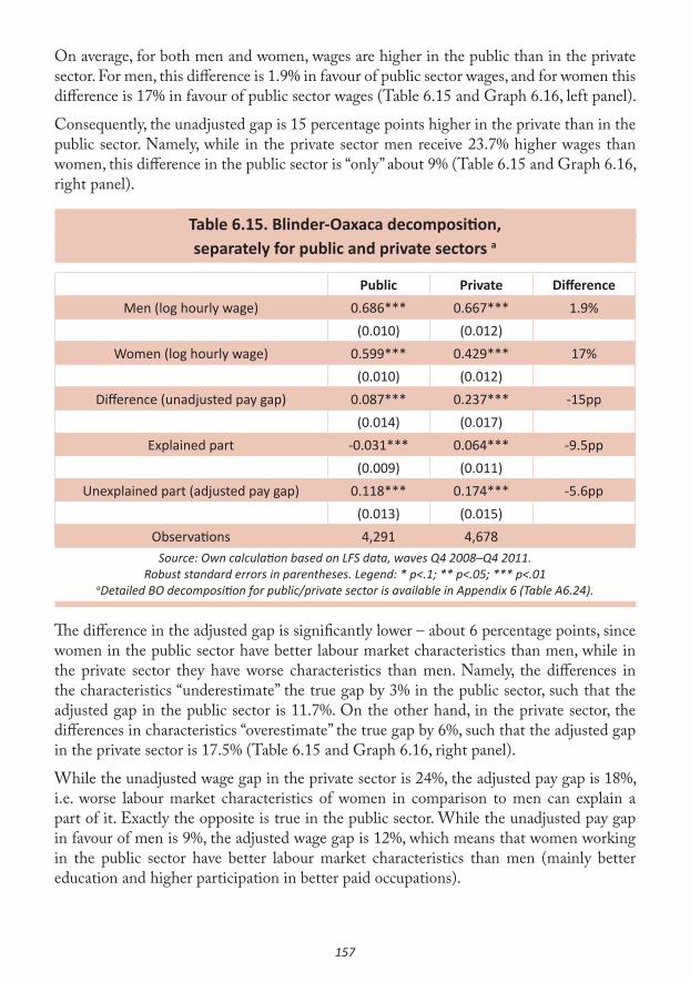
157

On average, for both men and women, wages are higher in the public than in the private sector. For men, this difference is 1.9% in favour of public sector wages, and for women this difference is 17% in favour of public sector wages (Table 6.15 and Graph 6.16, left panel).

Consequently, the unadjusted gap is 15 percentage points higher in the private than in the public sector. Namely, while in the private sector men receive 23.7% higher wages than women, this difference in the public sector is “only” about 9% (Table 6.15 and Graph 6.16, right panel).

Table 6.15. Blinder-Oaxaca decomposition,separately for public and private sectors a

Public Private DifferenceMen (log hourly wage) 0.686*** 0.667*** 1.9%

(0.010) (0.012)Women (log hourly wage) 0.599*** 0.429*** 17%

(0.010) (0.012)Difference (unadjusted pay gap) 0.087*** 0.237*** -15pp

(0.014) (0.017)Explained part -0.031*** 0.064*** -9.5pp

(0.009) (0.011)Unexplained part (adjusted pay gap) 0.118*** 0.174*** -5.6pp

(0.013) (0.015)Observations 4,291 4,678

Source: Own calculation based on LFS data, waves Q4 2008–Q4 2011.Robust standard errors in parentheses. Legend: * p<.1; ** p<.05; *** p<.01

aDetailed BO decomposition for public/private sector is available in Appendix 6 (Table A6.24).

The difference in the adjusted gap is significantly lower – about 6 percentage points, since women in the public sector have better labour market characteristics than men, while in the private sector they have worse characteristics than men. Namely, the differences in the characteristics “underestimate” the true gap by 3% in the public sector, such that the adjusted gap in the public sector is 11.7%. On the other hand, in the private sector, the differences in characteristics “overestimate” the true gap by 6%, such that the adjusted gap in the private sector is 17.5% (Table 6.15 and Graph 6.16, right panel).

While the unadjusted wage gap in the private sector is 24%, the adjusted pay gap is 18%, i.e. worse labour market characteristics of women in comparison to men can explain a part of it. Exactly the opposite is true in the public sector. While the unadjusted pay gap in favour of men is 9%, the adjusted wage gap is 12%, which means that women working in the public sector have better labour market characteristics than men (mainly better education and higher participation in better paid occupations).

158

Graph 6.16. Male and female log hourly wages (left panel)and wage gaps (right panel) in the private and public sectors

0,69 0,670,60

0,43

0,0

0,2

0,4

0,6

0,8

Public Private

Wages

Men Women

8,7%

23,7%

11,8%

17,4%

0,0%

5,0%

10,0%

15,0%

20,0%

25,0%

Public Private

Wage gap

Unadjusted gap Adjusted gap

Source: Own calculation based on LFS data, waves Q4 2008–Q4 2011.

Differences in characteristics in the public vs. the private sector

Graph 6.17 shows the most important labour market characteristics that “underestimate” or “overestimate” the pay gap in the public and the private sector. In the public sector, the most important effects are the effects of education (underestimate), sector of activity (overestimate), and region (underestimate). Better female position regarding these three characteristics underestimates or overestimates the true gap by 4, 2.4, and 1pp, respectively. In the private sector, the most important effects are the effects of tenure, occupation, and region. While tenure and occupation overestimate the true gap by 0.7pp and 5.9pp, regional effects underestimate the gap by 0.9pp.

Table 6.18 shows a detailed analysis of the explained part of the unadjusted gap in the public sector. In the public sector, the most important “positive” characteristics are: higher participation of women in high-paid jobs that require tertiary level of education (higher by 12.4 percentage points: 44.4% of women vs. 32% of men), jobs among Professionals (higher by 10.2 percentage points: 31.4% of women vs. 21.2% of men), and jobs among Technicians and associate professionals (higher by 11 percentage points: 31% of women vs. 20% of men. These three characteristics underestimate the true gap by 3.3, 1.1, and 0.5 percentage points, respectively (Table A6.24 in Appendix 6). Additional “positive” characteristics of women and their impact on the gap can be found in Table 6.18.

On the other hand, “negative” characteristics that work to overestimate the unadjusted pay gap are lower participation of women among high-paid jobs of Senior officials and managers (lower by 1.7 percentage points: 1.3% of women vs. 3% of men), lower participation of women in Industry (lower by 19.7 percentage points: 6.9% of women vs. 21.4% of men), as well as higher participation of women in low-paid jobs such as Clerical positions (higher by 5.2 percentage points: 18.3% of women vs. 13.1% of men), Elementary occupations (higher by 4 percentage points: 10.7% of women vs. 6.7% of men), and in Public administration, educa-

159

tion and health (higher by 20.3pp: 81.9% of women vs. 61.6% of men). If these characteristics of women were the same as those of men, the unadjusted gap would be lower.

Graph 6.17. Detailed Blinder-Oaxaca decomposition by sector of ownership – explained part – the impact of differences in characteristics

between the genders on the gender wage gap

-6 -4 -2 0 2 4 6 8

Educa�on

Tenure

Occupa�on

Sector of ac�vity

Region

Private Public

Source: Own calculation based on LFS data, waves Q4 2008–Q4 2011.

In total, “positive” characteristics of women in the public sector prevail over “negative” ones, so that the overall unadjusted gap is underestimated, i.e. it would be higher by around 3.1pp if women had the same characteristics as men. The most important “posi-tive” characteristics of women in the public sector, that underestimate the wage gap, are their higher participation in high-paid jobs (i.e. Professionals), as well as high-paid jobs which require tertiary level of education.

Table 6.19 shows detailed analysis of the explained part of the unadjusted gap in the private sector. In the private sector, “positive” characteristic of women is their lower participation in low-paid jobs with primary education only (lower by 3.1 percentage points: 4.5% of women vs. 7.6% of men). On the other hand, “negative” characteristics that work to over-estimate the unadjusted pay gap are lower participation of women among high-paid jobs of Senior officials and managers (lower by 1.2 percentage points: 2.3% of women vs. 3.5% of men), lower participation of women among the category Plant and machine operators (lower by 18.1 percentage points: 1.5% of women vs.19.6% of men), which belongs to a group of higher-paid job positions in private sector, as well as higher participation of women in low-paid jobs such as Clerical positions (higher by 4.4 percentage points: 14.1% of women, vs. 9.7% of men), Service and sales workers (higher by 26.8 percentage points: 49.6% of women vs. 22.8% of men), and in Public administration, education and health (higher by 4.5 percentage points: 10.4% of women vs. 5.9% of men). These characteristics overestimate the gap by 0.2, 0.2, 5.1, and 0.5 percentage points, respectively (Table A6.24 in Appendix 6). If these characteristics of women were the same as those of men, the unadjusted gap would be lower.

160

Table 6.18. Detailed Blinder-Oaxaca decomposition in the public sector – explained part – detailed impact of differences in characteristics

between the genders on the gender wage gap

High wage jobs Low wage jobs

Higher frequency of women

- Tertiary education (-3.3pp)- Professionals (-1.1pp)

- Technicians and associate professionals (-0.5pp)

- Central region (-0.1pp)- Coastal region (-0.1pp)

These characteristics make the true gap seem smaller.

- Clerks (0.3pp)- Elementary

occupations (1.2pp)- Public administration,

education and health (1.6pp)

These characteristics make the true gap seem smaller.

Lower frequency of women

- Senior officials and manage-rial positions (0.5pp)

- Manufacturing (1.1pp)

These characteristics make the true gap seem smaller.

- Primary education (-0.3pp)- Secondary

education (-0.3pp)- Agriculture (-0.1)- Service and sales workers (-0.3pp)

- Plant and machine operators (-0.5pp)

- Northern region (-0.7pp)

These characteristics make the true gap seem smaller.

Source: Own calculation based on LFS data, waves Q4 2008–Q4 2011.

In total, “negative” characteristics of women in the private sector prevail over “posi-tive” ones, such that the overall unadjusted gap is overestimated, i.e. it would be lower by 6.4pp if women had the same characteristics as men. The most important “negative” characteristic of women in the private sector, that overestimates the wage gap, is their higher participation in the low-paid Service and sales workers category (higher by 26.8 percentage points: 49.6% of women vs. 22.8% of men).

In the previous section we concluded that overall, unobservable differences explain the ad-justed gap better than the differences in returns to labour market characteristics. However, when we split the data, we find that in the public sector differences in returns account for the largest part of the adjusted gap, while in the private sector, the adjusted gap is better explained in the terms of unobservable heterogeneity. (Graph 6.20). These unobservable characteristics account for 32% of the adjusted pay gap in the public sector (3.8pp out of 11.8%) and 64% of the pay gap in the private sector (11.2pp out of 17.4%). Although

161

overall effects of unobservable characteristics are significant, separate effects of unobserv-able characteristics in the public and private sectors are not statistically significant, due to the smaller sample size when we split the overall sample into two. On the other hand, a detailed breakdown of the unexplained part of the wage differences (adjusted gap) between men and women shows significant differences in wage returns to labour market character-istics between public and private sectors. In what follows, we summarise these differences.

Table 6.19. Detailed Blinder-Oaxaca decomposition in the private sector – explained part – detailed impact of differences in characteristics

between the genders on the gender wage gap

High-paid jobs Low-paid jobs

Higher frequency of women

- Coastal region (-0.4pp)

These characteristics make the true gap seem smaller.

- Secondary education (0.2pp)- Clerks (0.2pp)

- Service and sales workers (5.1pp)- Public administration,

education and health (0.5pp)

These characteristics make the true gap seem smaller.

Lower frequency of women

- Senior officials and manage-rial positions (0.2pp)- Plant and machine

operators (0.9pp)

These characteristics make the true gap seem smaller.

- Primary education (-0.4pp)- Northern region (-0.5)

These characteristics make the true gap seem smaller.

Source: Own calculation based on LFS data from Q4 2008 to Q4 2011 (bi-quarterly data).

Differences in returns in the public vs. the private sector

In both the public and the private sector men have higher returns to education by around 2pp, which are, due to the smaller sample size, statistically insignificant. However, in abso-lute terms these differences are important for the explanation of the adjusted gap. Similarly, while in both sectors differences in returns to tenure are statistically insignificant, they are lower for women by 2.8pp in the private sector.

While in the private sector there are no overall differences in returns, in the public sector women have higher returns to occupational characteristics by 3.7pp. Most importantly, in the public sector, women have higher returns among Technicians and associate professionals

162

(by 2pp), Clerks (2pp), and lower returns among Service and sales workers (1.3pp) (Table A6.24 in Appendix 6).

In the private sector differences in returns on employment in different sectors of activity are higher for men by 2.4pp. Although statistically insignificant, these differences are high in absolute terms and are mainly caused by higher returns to Industry (by1.2pp) and Public administration, education and health (by 0.8pp).

On the other hand, women have lower returns to sector of activity characteristics in the public sector, by 8.2pp. Most importantly, in the public sector, women have lower returns in Industry (1.5%), and Public administration, education and health (7pp) (Table A6.24 in Appendix 6).

In conclusion, in the public sector, the adjusted gap is better explained in terms of differ-ences to returns to characteristics. On average, returns are higher for men, and account for the 68% of the adjusted gap (7pp out of 11.8%), while the differences in unobservable characteristics make 32% (3pp of 11.8%) of the gap. Most importantly, men have higher returns for working in Public administration, education and health.

In the private sector, the adjusted gap is better explained in terms of differences in unobservable characteristics, which make 64% of the gap (11.2pp out of 17.4%), while the differences in returns (in favour of men) make around 36% of the gap (6.2pp out of 17.4%). Although none of the differences in returns to characteristics where men have the advantage (education, tenure, sector of activity etc.) are statistically significant in them-selves, when grouped together, they manage to explain an important part of the gap.

Graph 6.20. Detailed Blinder-Oaxaca decomposition by sector of ownership – unexplained part – the impact of differences in returns to characteristics

and differences in unobservable characteristics between the genders on the gender wage gap (in percentage points)

-6 -4 -2 0 2 4 6 8 10 12

Educa�on

Tenure

Occupa�on

Sector of ac�vity

Region

Unobservablecharacteris�cs

Private Public

Source: Own calculation based on LFS data from Q4 2008 to Q4 2011 (bi-quarterly data).

163

Therefore, we may conclude that discrimination against women, in the form of lower returns to the same labour market characteristics than men, is more pronounced in the public sector. On the other hand, in the private sector, discrimination seems to stem from characteristics which we cannot observe with our data and which may have to do with the overall unequal position of women in the Montenegrin society, which increases their housework and care responsibilities at home, and therefore reduces their flexibility at the labour market. Furthermore, this finding is consistent with Becker’s hypothesis, surveyed in the literature review of this report, that increasing competition reduces discrimination by employers.

Differences at different points of the wage distributionin the public vs. the private sector

In this section we analyse the wage gap at the different points of the wage distribution in the public and private sectors separately. We split the sample into five wage brackets (quintiles) and compare differences in wages between men and women within these wage quintiles.

Both unadjusted and adjusted pay gaps are statistically significant at each of the five percentiles of the distribution in both sectors (Table A6.25 in Appendix 6). In the public sector, the explained part of the gap is significant in the 3rd, 4th and 5th quintile, while in the private only in the 5th quintile.

In the public sector, the gap is the highest in the 5th (top) quintile, but in the rest of the distribution it shrinks as wages grow. Namely, the unadjusted gap in the 1st quintile is 10.8%, it falls to around 6% in the 3rd and 4th quintile, where it reaches its minimum, and it rises to almost 15% in the top quintile. The adjusted gap follows the same pattern, but the differences between the quintiles are lower since the differences in characteristics widen the gap in the 3rd and 4th quintile (by 0.5pp and 1.1pp) to 5.9% and 6.2%, due to better female characteristics (better education on average). More importantly, the gap in the 5th quintile becomes lower by 4.3pp when adjusted for better male characteristics (Graph 6.21, left panel). Main male advantages in this quintile are better education and higher participation in better-paid occupations.

In the private sector, the gap widens towards the upper parts of the distribution. Namely, the unadjusted gap is the lowest in the 1st quintile of the distribution (16.8%), and it rises to almost 34% in the 5th quintile. The adjusted gap follows the same pattern since in all but the last quintile the differences in characteristics are statistically insignificant. In the top, 5th quintile, better characteristics of men lower the adjusted gap to 27.8% (Graph 6.21, right panel). Better male characteristics are mainly due to better occupational structure of men in this quintile (mainly their higher frequency among Professionals and Clerks).

164

Graph 6.21. Unadjusted and adjusted gap at different points in the wagedistribution in the public (left panel) vs. the private sector (right panel)

10,8%

7,1%5,3% 5,1%

15,3%

9,6%7,2%

5,9% 6,2%

11,1%

0%

5%

10%

15%

20%

1st 2nd 3rd 4th 5th

Public sector

unadjusted gap adjusted gap

16,8%19,7%

24,1% 25,7%

33,9%

16,2%19,8%

23,8% 25,5%27,8%

10%

15%

20%

25%

30%

35%

40%

1st 2nd 3rd 4th 5th

Private sector

unadjusted gap adjusted gap

Source: Own calculation based on LFS data from Q4 2008 to Q4 2011 (bi-quarterly data).

The adjusted gap in the public sector is significantly lower than the unadjusted gap in all parts of the wage distribution. This indicates the presence of a glass ceiling in both sectors, since the gap is the highest in the 5th quintile for both sectors. However, the glass ceiling effect is moderate, since the differences in the adjusted gap at the 5th quintile are not significantly higher compared to second highest gap (1st quintile for the public and 4th for the private sector). Interestingly, average wages are higher in the public sector in all quintiles, except for the 5th quintile of the male distribution, where the wages are higher by 15% for men who work in the private sector. This is the quintile in which we observe the highest unadjusted gap in all three countries (34%).

165

7. Comparing the gender pay gap across the three countries

In this chapter, we summarise and compare our findings on the gender pay gap trends across the three analysed countries. While we found many similarities in the distribution of male and female employment and wage gaps, a number of diverging trends were also observed. Given these differences, the countries of the Western Balkans cannot be treated as an entirely homogenous group when it comes to attempting to understand gender inequalities in the labour market. Country specific institutional frameworks as well as their historical path dependencies have also played a role in the shaping of gender relations in the economic sphere in this region.

7.1 Labour market trends and characteristics

In all three countries, female employment rates were significantly lower than male during the analysed period (2008-2011). The differences are the highest in Macedonia, where employment rate for men was higher by 18.6pp. In the other two countries, the employment gaps were slightly lower – amounting to 15pp in Serbia and 13.4pp in Mon-tenegro. The gaps in all three countries were slightly higher than in the EU-27, where the employment gap during the same period stood at an average of 12.4pp.

In all three countries, the employment gap is mainly caused by higher inactivity of women. In Macedonia women have higher inactivity rates than men by 26.8pp, in Serbia by 16.7 pp, and in Montenegro by 15.2 pp. Unemployment gaps in all the countries are very low, although women in all three countries have higher unemployment rates than men (in Macedonia by 0.8pp, in Montenegro by 1.8pp and in Serbia by 2.5pp). In comparison, the gender unemployment gap in EU 27 is non-existent.

Employment by educational attainment, age groups and type

In all three countries, gender employment gap shrinks with educational attainment. The gap is the highest among those with primary education (24pp in Macedonia, 15pp in Montenegro, 17pp in Serbia); it shrinks at the secondary level of education in Macedonia and Montenegro, but not in Serbia (13pp in Macedonia, 12pp in Montenegro, 17pp in Serbia), and it is the lowest (8 pp in Macedonia) or totally diminished among those with tertiary educational attainment (there is no gender gap in Serbia, nor in Montenegro, among women and men with tertiary education).

The substantial gender employment gap between the most educated women and men (66% vs. 74%) in Macedonia at first glance seems somewhat surprising. However, while the most educated individuals are most frequently employed in the public sector, legally regulated affirmative action in Macedonia has also resulted in the increase of employment of repre-sentatives of ethnic minorities in the public sector, from 5.6 to 24.2% between 2004 and 2010 (CRPM 2012, p. 41-42). Albanians are the largest ethnic minority in Macedonia, and

166

female individuals of Albanian origin are associated with 35% lower probability of partici-pating in the labor force than female individuals of Macedonian origin. Also, traditional norms related to female employment and the patriarchal “male breadwinner” household model are still prevalent in Albanian communities (World Bank 2008). Therefore, affirma-tive action towards inclusion of ethnic minorities in the public sector could have had a negative impact on the gender gap between employees in the public sector. Furthermore, since employment in the public sector is highly sought after among educated women for its perceived security and family friendly working hours, women with tertiary education may engage in wait unemployment (i.e. wait for a placement in the public sector) more frequently than other population groups.

Given the rather high gender gap in employment among those with tertiary education in Macedonia, it is quite surprising to observe the smallest employment gap of all three countries among those with secondary education. Furthermore, in Macedonia, the gender employment gap for those with the lowest educational attainment is much more pro-nounced than in the other two countries. Such pronounced gender gap in employment for those with the lowest educational attainment is somewhat surprising, since these employ-ment figures include all those employed as unpaid contributing family members, which is the most common form of employment for women with low education, especially in rural areas.

On the other hand, employment gaps by age groups do not vary much across the three countries, with the largest gaps in employment between the genders (above 20pp) found among the oldest cohort of the working age population (55-64 years of age) and the small-est gap between the genders (below 10pp) among the youngest population cohort (15-25). However, the youngest working age population cohort has by far the lowest employment levels for both genders, both due to higher inactivity (because of education) and higher unemployment. On the other hand, the pronounced gap among the oldest working age cohort reflects the fact that women tend to retire (or withdraw from the labour market) earlier than men in all three countries.

Compared to men, women in all three countries are more often found in wage employ-ment than men (75% of women and 70% of men in Serbia, 77% of women and 70% of men in Macedonia, and 89% of women and 79% of men in Montenegro). However, although a higher percentage of employed women are in wage employment than men, women are a minority in total wage employment in all three countries (43% of total em-ployment in Serbia, 41% in Macedonia and 46% in Montenegro).

On the other hand, women can less frequently be found working as self-employed in all three countries (13% vs. 26% of men in Serbia, 8% vs. 24% of men in Macedonia, and 10% vs. 20% of men in Montenegro). In Serbia and Macedonia they are found to work a lot more frequently as unpaid family members (12% vs. 4% of men in Serbia, and 14% vs. 6% of men in Macedonia), most often in agriculture. This difference may be due to the fact that men who work on their own agricultural land tend to report themselves as self-employed while women tend to report themselves as unpaid family members, which results in another form of gender inequality in the economic sphere – men’s and women’s unequal

167

access to resources obtained through joined labour. On the other hand, in Montenegro there is no difference between men’s and women’s engagement as unpaid family members, and unpaid family members represent a very rare type of employment there (1% of each gender).

Employment before and after the economic crisis

Of the three countries, Serbia had a slightly higher employment rate for both genders at the onset of the economic crisis (in 2008). However, both its male and female em-ployment rates suffered a significant negative impact by the crisis, which was not the case in the other two countries. While male employment rate dropped by 10pp, female dropped by almost 7pp (in Serbia). The male employment rate in Montenegro dropped as much as in Serbia (by 10pp), while female employment rate was much more stable, i.e. its level remained almost unchanged during the crisis. At the same time, during this period, employment rates for both genders in Macedonia slightly increased (Q4 2008–Q4 2011). Yet, since employment rates for both genders were initially lower than in Montenegro and Macedonia than in Serbia, the new post-crisis employment levels have almost converged in all three countries (male: 52% in Serbia, 49% in Montenegro and 52% in Macedonia; female: 38% in Serbia, 42% in Montenegro and 34% in Macedonia).

These diverging labour market responses to the economic crisis could reflect the different stages of transition these three countries were in when the crisis hit, which could have affected trends in demand for labour. For example, Macedonia embarked on company restructuring and privatisation (which entailed shedding of excess labour) much earlier than Serbia and Montenegro, which were under economic sanctions throughout the 1990’s. This could have been the reason why employment levels for both genders at the onset of the crisis in Macedonia were lower than in the other two countries. Furthermore, elasticity of employment to GDP during the crisis in Serbia stood at 2.6, which by far exceeded elasticities observed in the neighbouring economies (FREN 2010, p. 20). Such high elasticity of employment to GDP indicates that the crisis sped up the unfinished process of enterprise restructuring and economic transition.

The shrinking of the employment gap may also be due to the overrepresentation of women in the public sector in the countries of the Western Balkans. Namely, while the private sector adjusted to the crisis through job loss, the public sector adjusted through real wage contraction which helped it to maintain employment levels. Therefore, more women than men may have kept their jobs during the crisis.

The narrowing of gender employment gaps in all three countries seems to confirm our hypothesis that the crisis had a stronger negative impact on male than female employment (although not as pronounced in Montenegro as in the other two countries). Therefore, we may expect these gaps to grow back to pre-crisis levels as soon as the masculinised sectors of the economy recover.

168

7.2 Gender differences in characteristics: unadjusted vs. adjusted wage gap

The unadjusted gender wage gap represents the difference in mean log hourly wages be-tween men and women. However, the two genders in all three countries differ significantly according to characteristics and skill levels of women and men who work, i.e. an average employed woman is not identical to an average employed man by level of education, work experience, occupation, industry sector, etc. Therefore, the adjusted wage gap between the genders (obtained by reweighing the gender wage gap so that it reflects these differences in characteristics) is a much more relevant indicator of the gender wage gap.

In order to illustrate this point, we can observe that the share of women among all wage employees with tertiary education is 49% in Macedonia, 51% in Montenegro and 55% in Serbia. The differences become more pronounced among those working with secondary education, where only 40%, 43% and 41% of all wage employees in Macedonia, Montene-gro and Serbia respectively are women. Among wage employees with primary education, only 33%, 35% and 39% in Macedonia, Montenegro and Serbia respectively are women.

Graph 7.1 below shows unadjusted and adjusted gender gaps for all three countries. When gender differences in labour market characteristics are taken into account, the gap widens in Serbia and Macedonia, while it stays at the same level in Montenegro.

Graph 7.1. Unadjusted and adjusted gender wage gaps in Serbia, Macedonia and Montenegro

03%

13%

16%

11%

18%16%

00%

05%

10%

15%

20%

Serbia MontenegroMacedonia

Unadjusted gap Adjusted gap

Source: Own calculations from LFS data, 2008-2011.

Therefore, unlike the trends we observe in Western economies, where working women on average have worse educational attainment, work experience and job related characteristics than men, due to historical discrimination (see Chapter 2), the differences in labour mar-ket characteristics between men and women cannot explain the gender wage gap in the Western Balkans.

169

In fact, in Serbia and Macedonia these differences in characteristics hide the true mag-nitude of the gap, because employed women in the two countries on average have better characteristics than employed men (this is to a great extent due to the fact that women with the worst labour market characteristics are unemployed or inactive, i.e. discriminated at the point of entry into wage labour, rather than discriminated through lower wages). In other words, the explained part of the wage gap is negative: as soon as we try to explain the existence of the gap, we end up with an even larger gap.

Observed in greater detail, in both Serbia and Macedonia, this female advantage is split between their better education and better occupational characteristics (such as occupation and sector of activity)89. This suggests that women in Serbia and Macedonia “use” their better personal labour market characteristics, such as education, to obtain jobs in the more highly paid occupations and sectors. However, they are not paid as well as men within these highly paid occupations and sectors.

In Montenegro, a different trend is observed. When we control for gender differences in education and work experience with the same employer (tenure), the estimated gender pay gap amounts to 19.2%. However, when we add occupation, sector of activity and region, the gender pay gap shrinks to 16.1% in favour of men. The fact that the wage gap grows to 19.2% when we include only education and tenure into the equation, and it drops down to 16.1% when we add job characteristics, can suggest the following: while employed women have better personal labour market characteristics than employed men, they do not, or are not at all able to, “use” these characteristics in order to access the better paid occupations and sectors of the economy. Therefore, men are better positioned regarding the occupation and sector of activity then women, i.e. they work in better paid occupations and sectors.

As shown in Graph 7.1, the unadjusted gender wage gap is the most pronounced in Montenegro. The highest unadjusted gap in Montenegro may be due to the strong tourism sector and the consequentially higher female employment in the private sector, including tourism (Montenegro has the lowest employment and inactivity gap of all three countries). As we have concluded from our analysis, low unadjusted gender wage gaps in the Western Balkans in comparison to Western countries are the consequence of low female labour market participation, especially among those with “worse” labour market characteristics. As more women with worse labour market characteristics enter the labour market, we can expect the unadjusted wage gap to widen. Therefore, it is intuitive to observe the largest unadjusted wage gap in the country with the lowest employment gap.

On the other hand, the true, or adjusted, gap is the most pronounced in Macedonia. As the adjusted gap refers to differences in wages between individuals with the same labour market characteristics (men and women with the same educational attainment and work experi-ence and those working in the same occupation/sector of the economy), it can be ascribed to labour market discrimination. In other words, while the high wage gap in Montenegro exists due to greater diversification of women across occupations and sectors of activity, and possibly their “ghettoisation” into female occupations and sectors, in Macedonia,

89 See sections 4.2.1 and 5.2.1 in country chapters for a more detailed account of differences in characteristics.

170

discrimination within occupations and sectors of activity is more dominant. This may be due to the fact that female unemployment is a lot more pronounced in Macedonia than in the other two countries, while female employment is lower than in the other two. This excessive female labour supply in Macedonia may be lowering female wages vis-à-vis male within the same occupations/sectors to a greater extent than this is the case in the other two countries. Furthermore, while we have observed higher female wages in the public than in the private sector in all three countries, female access to the Macedonian public sector may be more limited than in the other two countries, so they may be willing to accept lower wages. This is possibly due to affirmative action towards equal representation of ethnic minorities in the public sector which we discuss at the beginning of this chapter.

Gender differences in returns to characteristics: the adjusted wage gap

The adjusted wage gap is the gap which remains unexplained after we take into consid-eration the above discussed differences in characteristics between employed women and employed men. The adjusted gap exists because of: i) labour market discrimination against women, in a sense that there are differences between the genders in returns to the same labour market characteristics, and ii) unobserved heterogeneity of workers’ characteristics, which we were not able to capture through variables such as education, work experience, occupation, etc. These could vary from characteristics such as, for example, women be-ing less flexible in terms of working hours or business trips due to housework and care responsibilities, to other effort- and ability-related variables which we do not (or cannot) measure, as well as labour market frictions.

In all three countries the adjusted gap is better explained by differences in unobservable characteristics, than by differences in returns to observable labour market characteristics.

In Serbia, the adjusted gender wage gap cannot at all be explained by differences in returns to observable characteristics, so the entire adjusted gap exists due to different returns between men and women on unobservable characteristics.

In Macedonia, the largest share of the adjusted wage gap – 69% (12.5pp of 17.9%) stems from unobservable characteristics of workers. On the other hand, differences in returns to personal labour market characteristics and occupation account for 31% of the unexplained wage gap (5.4pp of 17.9%). Women in Macedonia, on average, have lower market re-turns to education, occupation and sector of activity.

In Montenegro, differences between the genders in returns to the same labour market characteristics account for 25% of the adjusted gap (4.1pp of 16.1%). On the other hand, 75% of the adjusted gender wage gap (12pp of 16.1%) cannot be accounted for by differ-ent returns. This means that there is some other unobservable heterogeneity between the genders, which leads to the wage gap.

171

7.3 Gender wage gap in the public vs. the private sector

In all three countries the gender wage gap is better explained when the sample of the analysis is split into public vs. private sector. This is due to strong labour market duality in the Western Balkans, where the public and the private sectors operate under differ-ent “rules.”

Before focusing on the wage gap, it is important to note that wages are higher in the public sector in all three countries. Furthermore, this public sector wage premium is higher for women than for men (Graph 7.2). The difference in wages between the sectors is lowest in Montenegro (17.0% for women and 1.9% for men). The differences are much higher in Serbia and Macedonia, where men have around one-third lower wages when working in the private sector then when working in the public (34.5% for Serbia, 32.6% for Macedonia), while the difference for women is even higher (42.2% in Serbia; 46% in Macedonia).

Similarly to the results obtained from the analysis of the entire sample, the unadjusted wage gaps for both sectors are the highest in Montenegro (23.7% in the private and 8.7% in the public), followed by Macedonia (17.7% in the private and 4% in the public), while they are the lowest in Serbia (9.4% in the private and 1.6% in the public).

Additionally, unadjusted wage gaps are significantly higher in the private than in the public sector in all three countries (Graph 7.2, right panel). Differences in unadjusted gaps between the private and the public sector range from 15pp in Montenegro (23.7% in the private vs. 8.7% in the public), to 13.7pp in Macedonia (17.7% vs. 4%), and 7.8pp in Serbia (9.4% vs 1.6%).

Graph 7.2. Public sector wage premiuma (left panel) and unadjusted wage gap,public vs. private sector (right panel)

35%

02%

33%

42%

17%

46%

0%

10%

20%

30%

40%

50%

Serbia Montenegro Macedonia

Public sector wage premium

Men Women

1,6%

8,7%

4,0%

9,4%

23,7%

17,7%

0%

5%

10%

15%

20%

25%

Serbia Montenegro Macedonia

Unadjusted wage gap

Public Private

a Public sector wage premium is a percentage difference between wages in the public and private sector. Source: Own calculations from LFS data, 2008-2011.

Adjusted gaps in the public sector are larger than the unadjusted ones in all three countries, which means that the better female labour market characteristics in this sector hide the

172

true extent of the wage gap when we look at the simple difference in wage averages between the genders. Gender differences in labour market characteristics in the public sector are significant and in favour of women in all three coutries (Graph 7.3, left panel, blue bars), so they act to underestimate the adjusted wage gap. Therefore, our analysis suggests a lot higher extent of wage discrimination of women in the public sector than a simple comparison of average wages would suggest.

Graph 7.3. Differences in characteristics (left panel, in pp) and the adjustedwage gap in public and private sector, by country

-5,8-3,1

-7,4

-1,7

6,4

-0,8

-10

-5

0

5

10

Serbia Montenegro Macedonia

Differences in charateris�cs

Public Private

7,5%

11,8% 11,4%11,0%

17,4% 18,5%

0%

5%

10%

15%

20%

Serbia Montenegro Macedonia

Adjusted wage gap

Public Private

Source: Own calculations from LFS data, 2008-2011.

In the private sector, differences in labour market characteristics (Graph 7.3, left panel, red bars) are either very slightly in favour of women (in Serbia and Macedonia), or signficantly in favour of men (in Montenegro). Because of these differences in characteristics, the adjusted gap in Serbia and Macedonia is slightly higher than than the unadjusted gap. The opposite stands for Montenegro – the explained part of the gap is positive. The private sector in Montenegro (with tourism’s strong share) therefore follows much more closely Western trends, where women have worse labour market characteristics than men (due to historical disadvantages), which explain a part of their differences in earnings.

In summary, within the public sector, better labour market characteristics of women substantially underestimate the wage gap in all three countries. On the other hand, in the private sector, female labour market characteristics are either only slightly better than male, so they have no substantial impact on the gap (in Serbia and Macedonia), or they are significantly worse, so they overestimate the gap (in Montenegro). In other words, after adjusting for differences in labour market characteristics, in all three countries the differences between the wage gaps in public and private sector become smaller. They now range from 7.4pp (18.5% vs 11.4%) in Macedonia, over 5.6pp in Montenegro (17.4% vs 11.8%,), to 3.5pp in Serbia (9.4% vs 1.6%).

Adjusting for labour characteristics shows that the effect of discrimination in the public sector is not as large as in the private sector, but that it is far from non-existent.

173

The adjusted gender wage gap in the public sector

In the public sector, the adjusted gender wage gap in Serbia of 7.5% is lower than in the other two countries. The adjusted public sector gender wage gaps in Macedonia and Montenegro stand at 11.4 and 11.7% respectively (Graph 7.3, right panel).

There are some differences in the sources of public sector discrimination of women across the three countries.

In Serbia women actually have higher returns to the same labour market characteristics than men when working in the public sector (by 4pp on average). However, male unobservable characteristics are better awarded than female and they seem to be the main culprit for the existence of the wage gap between the two genders in the public sector. What happens is that this negative effect of better male returns to unobservables is somewhat lessened by the fact that women have better returns to observables. If the differences in returns to characteristics were the same, the adjusted gender wage gap in the public sector in Serbia would be at the same level as in the private sector in Serbia, and at the same level as in the public sectors of Macedonia and Montenegro (11%).

In Macedonia, women have almost equal returns to characteristics as men in the public sector, so the main source of discrimination is higher male returns to unobservable char-acteristics (10.6pp of 11.4% gap is due to differences in unobservable characteristics). This effect is more dominant in Macedonia than in Serbia, especially because it is not even partially offset by better female returns to observables, like it is the case in Serbia. However, the effect of discrimination in Macedonia is a lot stronger in the private sector, so we can still say that women are less discriminated in the public than in the private sector.

In Montenegro we observe a completely different trend. The adjusted wage gap is better explained by differences to returns. On average, returns are higher for men, and account for 68% of the adjusted gap (7pp out of 11.8%), while the differences in unobservable characteristics make 32% (3pp of 11.8%) of the gap. This suggests that women cannot access the best paid occupations and sectors of activity within the public sector, regardless of their better personal labour market characteristics such as the level of education.

Looking at the gender gap across the wage distribution in the public sector, different trends emerge. While in Serbia the adjusted gap seems to be equally pronounced at all levels of the wage distribution in the public sector (between 4 and 5%), in Macedonia there is a clear glass ceiling effect, where the most pronounced gender difference in wages comes at the top of the wage distribution (the gap is 7%), i.e. women are unable to access the top paid professions. Montenegro has the most pronounced adjusted gender wage gap at the top of the wage distribution in the public sector, at above 15%, implying a much stronger glass ceiling effect than in the other two countries. Furthermore, in Montenegro there is a pronounced wage gap also at the bottom of the distribution (and it is more moderate in the middle of the distribution), which implies that women with the lowest wages also earn substantially less than men with the lowest wages in the public sector. This wage floor effect does not seem to be very dominant in the public sector of the other two countries.

174

The adjusted gender wage gap in the private sector

In Serbia, differences in returns are on average higher for men in the private sector. While gender differences in returns to the same labour market characteristics can account for 42% of the adjusted gap, the differences in unobservable characteristics can account for the remaining 58%. While the private sector in Serbia seems to be characterised by more explicit discrimination than the public sector, due to the presence of lower returns to characteristics for women, this could also be the case because there are more sectors of activity and occupations within the private than within the public sector, so the wage dispersion is wider. Therefore, these differences may reflect different values added of the different sectors to the economy, rather than be due to the fact that private employers discriminate more. However, this leads us to a question why women seem to be over-represented in the less paid occupations and sectors of the economy, which also needs to be acknowledged as a form of discrimination.

In Macedonia, the largest part of the adjusted gender wage gap in the private sector exists due to the unobservable characteristics between men and women, which account for 80% of the adjusted pay gap in the private sector (14.7pp out of 18.5%). The rest of the unex-plained gap (20%) occurs because of different returns to observable personal characteristics of labour market participants.

In Montenegro, the adjusted wage gap is better explained by differences in unobservable characteristics, which make 64% of the gap (11.2pp out of 17.4%), while the differences in returns (in favour of men) make around 36% of the gap (6.2pp out of 17.4%).

In Serbia, looking at the wage distribution in the private sector, differences in characteristics affect the adjusted wage gap differently across the quintiles: while it is still the lowest at the bottom part of the distribution, it is the highest at the top of the distribution, suggesting a glass ceiling effect, which means that it is more difficult for women to access the best paid positions in the private sector.

In Macedonia, in the private sector, gender wage gaps are consistently large across the entire distribution, so the glass ceiling effect does not seem to particularly stand out, due to the generally much better rewards for men than for women at all levels of the wage distribution.

In Montenegro, we observe a very pronounced glass ceiling effect, with the largest gender wage gap of 28% existing at the top of the wage distribution. Although the wage gap at the bottom of the wage distribution is almost half of the wage gap at the top, at 16.2% it is still almost as high as in Macedonia and much higher than in Serbia.

175

8. Policy Implications

Our findings on the composition of the gender wage gap in the Western Balkans have several important implications for government policies aiming to address economic in-equalities between men and women.

1. Counter to widely held beliefs, separate analyses of the public and private sectors uncover that pay discrimination of women is not much higher in the private than in the public sector. However, gender pay disparities are more “hidden” in the public sector, because women who work in it have much better labour market characteristics than men who do. If there were no discrimination, women would have higher average wages than men in the public sector, because they are on average better qualified. In other words, women need to have better labour market characteristics than men to access the same positions in the public sector at all levels of responsibility, which can be considered a dis-criminatory practice. This effect seems particularly pronounced at the top part of the wage distribution, meaning that women have the most difficult time accessing the best-paid positions in the public sector, although they may be better qualified for those jobs than their male counterparts.

2. Women seem to be more “punished” in the public than in the private sector90 for their “worse” unobservable characteristics, e.g. for the fact that they may be less flexible in terms of working hours or business trips due to housework and care responsibilities or the fact that they may be perceived by employers as less able to perform certain jobs (e.g. due to prejudice/patriarchal beliefs that women are less suited for positions of author-ity). This could be seen as a surprising finding, since the public sector is traditionally held to offer better non-pecuniary benefits and work-life balance than the private sector. On the other hand, in light of the hypothesis (proved empirically on a number of occasions) that increasing competition reduces the taste for discrimination by employers, we can also say that the public sector can “afford” to indulge in their taste for discrimination more than the private sector.

3. Although we see a wider true wage gap between the genders in the private sector, we need to consider the fact that the private sector consists of a wider range of activities and occupations. We also need to consider that women have traditionally been trained for the lower paid and undervalued occupations and treated as secondary workers. In that sense, since market competition does not exist in a vacuum, the wage gap observed in the private sector may reflect labour market rigidities such as horizontal occupational segregation and larger frictions in female job search than male. In that sense, interventions at the level of education and training may also influence future trends in gender wage gaps.

4. Due to the fact that transition from socialist to capitalist economy has not been completed yet, especially in Serbia and Montenegro, it is not entirely clear what the new equilibrium in economic relations between the genders will be at the end of it (if

90 Meaning that better male returns to unobservable characteristics play a larger role in explaining the gender pay gap in the public than in the private sector.

176

there is an end point at all). Both Serbia and Montenegro are still expected to conduct painful public sector reforms and it is not clear upfront which gender will be more hit by these reforms. Careful ex-ante gender analyses of envisaged reforms could answer some of these questions.

5. The economic crisis has resulted in the shrinking of the gender wage and employment gap in all three countries. However, this cannot be seen as good news, since it is a result of the more pronounced negative impact of the crisis on the masculinised sectors than the feminised ones. The question of permanence of these trends therefore remains pertinent. Once masculinised sectors of the economy recover and possibly become more produc-tive as a result of the crisis (so that wages go up in these sectors), we may see the recovery of pre-crisis gaps, or potentially even their worsening.

177

Bibliography

— Altonji, J. G. & Blank, R. M. (1999). “Race and Gender in the Labour Market.” In Handbook of Labour Economics, O. Ashenfelter & D. Card (Eds.), Vol.3, Ch.48 (pp. 3143-3259). Elsevier Service B.V.

— Angel-Urdinola, D. F. (2008). “Can the Introduction of a Minimum Wage in FYR Macedonia Decrease the Gender Wage Gap?” (Social Policy Discussion Paper No. 0837). Washington DC: World Bank.

— Angel-Urdinola, D. F. & Macias, V. (2008). “FYR Macedonia Labour Market Profile 2004-2007: A Policy Note” (Human Development Sector Unit, Europe and Central Asia). Washington, DC: World Bank.

— Antonczyk, D., Fitzenberger, B. & Sommerfeld, K. (2010). “Rising Wage Inequality, the Decline of Collective Bargaining, and the Gender Wage Gap.” Labor Economics, 17(5), 835-847.

— Arandarenko, M. & Avlijaš, S. (2011). “Behind the veil of statistics: Bringing to light structural weaknesses in Serbia.” In V. Schmidt, & D. Vaughan-Whitehead (Eds.), The Impact of the Crisis on Wages in South-East Europe (pp. 123-158). International Labour Organization.

— Arulampalam, W., Booth, A. L., & Bryan, M. L. (2007). “Is There a Glass Ceiling over Europe? Exploring the Gender Pay Gap across the Wage Distribution.” Industrial and Labor Relations Review, 60, 163-186.

— Babcock, L., & Laschever, S. (2003). Women Don’t Ask: Negotiation and the Gender Di-vide. Princeton: Princeton University Press.

— Bayard, K. & Hellerstein, J. (2003). “New Evidence on Sex Segregation and Sex Dif-ferences in Wages from Matched Employee-Employer Data.” Journal of Labor Economics, 21-4, 887-921.

— Black, S. E. & Brainerd, E. (2004). “Importing Equality? The Effects of Increased Com-petition on the Gender Wage Gap.” Industrial and Labor Relations Review, 57, 540-559.

— Blau, F. D. (1996). “Where are we in the economics of gender? The gender pay gap” (NBER Working Paper Series, 5664). Cambridge, MA: National Bureau of Economic Research.

— Blau, F. D. & Kahn, L. M. (1997). ”Swimming Upstream: Trends in the Gender Wage Differential in the 1980’s.” Journal of Labour Economics, 15, 1-42.

— Blau, F. D. & Kahn, L. M. (2000). “Gender Differences in Pay.” Journal of Economic Perspectives, 14, 75-99.

— Boraas, S. & Rodgers, W. M. III (2003). “How does gender play a role in the earnings gap? An update.” Monthly Labor Review, March, 9-15.

178

— Bertrand, M., Goldin, C. & Katz, L. F. (2009). “Dynamics of the gender gap for young professionals in the financial and corporate sectors” (NBER Working Paper No. 14681). Cambridge, MA: National Bureau of Economic Research.

— Bertrand, M (2011). “New Perspectives on Gender”. In O. Ashenfelter & D. Card (Eds.), Handbook of Labor Economics, Vol. 4B (pp. 1543-1590). Elsevier B.V.

— Blinder, A. S. (1973). “Wage Discrimination: Reduced Form and Structural Estimates.” The Journal of Human Resources, 8(4), 436-455.

— Blunch, N.-H. & Sulla, V. (2010). “The Financial Crisis, Labor Market Transitions and Earnings: A Gendered Panel Data Analysis for Serbia” (Poverty Reduction and Economic Management Unit, Europe and Central Asia Region Department). Washington, DC: World Bank.

— Blunch, N.-H. (2010) “The Gender Earnings Gap Revisited: A Comparative Study for Serbia and Five Countries in Eastern Europe and Central Asia” (Poverty Reduction and Economic Management Unit, Europe and Central Asia Region Department). Washing-ton, DC: World Bank.

— Brainerd, E. (2000). “Women in Transition: Changes in Gender Wage Differentials in Eastern Europe and the Former Soviet Union.” Industrial and Labor Relations Review, 54, 138-162.

— Buchinksy, M. (1994). “Changes in the U.S. Wage Structure 1963-1987: Application of Quantile Regression,” Econometrica 62(2), 405-458.

— Chase, R. S. (1995). “Women’s Labor Force Participation During and After Commu-nism: A Study of the Czech Republic and Slovakia” (Economic Growth Center Discussion Paper No. 768). New Haven: Yale University. Retrieved July 20, 2012, from http://aida.wss.yale.edu/growth_pdf/cdp768.pdf

— Chase, R. S. (1998). “Markets for Communist Human Capital: Returns to Educa-tion and Experience in the Czech Republic and Slovakia.” Industrial and Labor Relations Review, 51:3, 401-423.

— Chernozhukov, V., Fernández-Val, I. & Melly, B. (2008). “Inference on counter-factual distributions” (Department of Economics – Working Papers Series WP2008-005). Bos-ton, MA: Boston University. Retrieved March 30, 2012, from http://people.bu.edu/ivanf/wp_files/counterfactuals-may-21-2008.pdf

— CRPM (2012). “How to eliminate discrimination in the public sector?“ Skopje, Mace-donia: Center for Research and Policy Making. Retrieved February 20, 2013, from http://www.crpm.org.mk/wp-content/uploads/2012/03/How-to-eliminate-discrimination-in-the-public-sector.pdf

— Cueto, B. & Sanchez-Sanchez, N. (2010). “Occupational segregation as a cause of gender-based salary differences. A sectoral analysis” (Working Paper, Encuentros de Eco-nomia Aplicada, Asociacion Libre de Economia, Spain). Retrieved July 21, 2012, from http://www.alde.es/encuentros/anteriores/xiiieea/trabajos/pdf/139.pdf

179

— Echrenberg, R. G. & Smith, R. S. (2003). Modern Labor Economics: Theory and Public Policy (8th edition). Pearson Education, Inc.

— Eurostat (2010). Europe in figures: Eurostat Yearbook 2010. Brussels: European Com-mission.

— Floro, M. (2000). “Financial Crisis, Gender, and Power: An Analytical Framework.” World Development 28:7, July, 269-1283.

— Foubert, P. (2010). “The Gender Pay Gap in Europe from a Legal Perspective” (report commissioned by the European Commission). Luxemburg: Publications Office of the European Union. Retrieved March 20, 2012, from http://ec.europa.eu/justice/gender-equality/files/gender_pay_gap/genderpaygapfromlegalperspective-nov2010_en.pdf

— Grajek, M. (2003). “Gender Pay Gap in Poland.” Economics of Planning, 36, 23-44.

— Harkness, S. & Evans, M. (2011). “The Employment Effects of Recession on Couples in the UK: Women’s and Household Employment Prospects and Partners’ Job Loss.” Journal of Social Policy 40:4, October, 675-693.

— Heckman, J. J. (1976). “The Common Structure of Statistical Models of Truncation, Sample Selection and Limited Dependent Variables and a Simple Estimator for Such Models.” Annals of Economic Social Measurement, 5(4), 475-492.

— Heckman, J. J. (1979). “Sample Selection Bias as a Specification Error.” Econometrica, 47(1), 153-161.

— Heinze, A. & Wolf, E. (2010). “The intra-firm gender wage gap: a new view on wage differentials based on linked employer–employee data.” Journal of Population Economics, 23, 851–879.

— Hunt, J. (2002). “The transition in East Germany: when is a ten point-fall in the gender gap bad news?” Journal of Labor Economics, 20, 148-169.

— Jann, B. (2008). “The Blinder-Oaxaca Decomposition for Linear Regression Models.” The Stata Journal, 8(4), 453-479.

— Jones, D. C. & Ilayperuma, K. (1994). “Wage Determination Under Plan and Early Transition: Evidence from Bulgaria” (Department of Economics Working Paper Series). Hamilton, N.Y: Hamilton College. Retrieved March 20, 2012, from http://academics.hamilton.edu/economics/home/workpap/04_09.pdf

— Jurajda, S. & Paligorova, T. (2009). ”Czech female managers and their wages.” Labour Economics, 16, 342-351.

— Jurajda, S. (2003). “Gender wage gap and segregation in enterprises and the public sector in late transition countries.” Journal of Comparative Economics, 31, 199-222.

— Killingsworth, M. R. (1983). Labor Supply. Cambridge: Cambridge University Press.

— Kim, H. & Voos, P. B. (2007). “The Korean economic crisis and working women.” Journal of Contemporary Asia, 37:2, 190-208.

180

— Koenker, R. & Bassett, G. (1978). “Regression Quantiles,” Econometrica, 46(1), 33–50.

— Krstić, G. & Reilly, B. (2000). “The gender pay gap in the FRY.” Ekonomska misao, 33 (3-4), 191-213.

— Krstić, G. & Sanfey, P. (2011). “Earnings inequality and the informal economy. Evidence from Serbia.” Economics of Transition, 19(1), 179–199.

— Leibbrandt, A. & List, J. A. (2012). “Do Women Avoid Salary Negotiations? Evidence from a Large Scale Natural Field Experiment” (NBER Working Paper No. 18511). Cam-bridge, MA: National Bureau of Economic Research.

— Levanon, A., England, P. & Allison, P. (2009). “Occupational Feminization and Pay: Assessing Causal Dynamics Using 1950-2000 U.S. Census Data.” Social Forces, 88(2), 865-892.

— Ludsteck, J. (2010). “Occupational Segregation within Establishments and the Gender Wage Gap” (preliminary draft, IAB Nuremberg). Retrieved April 15, 2012, from http://extranet.isnie.org/uploads/isnie2010/ludsteck.pdf

— Łobodzińska, B. (Ed.). (1995). Family, Women, and Employment in Central-Eastern Europe. Westport, CT: Greenwood Press.

— Machado, J. & Mata, J. (2005). “Counterfactual Decomposition of Changes in Wage Distributions using Quantile Regression.” Journal of Applied Econometrics, 20(4), 445–465.

— Maddala, G. S. (1983). Limited-Dependent and Qualitative Variables in Econometrics. Cambridge: Cambridge University Press.

— Manning, A. (2011). “Imperfect Competition in the Labor Market.” In O. Ashenfelter, & D. Card (Eds.), Handbook of Labor Economics, Vol. 4B (pp. 973-1041). Elsevier B.V.

— Mincer, J. (1974). Schooling, Experience and Earnings. Columbia University Press, New York.

— Mincer, J. (1993). Studies in Human Capital: Collected Essays of Jacob Mincer. Vol. 1, Part I. Cambridge: Edward Elgar.

— Mojsoska-Blaževski, N. (2011). “The former Yugoslav Republic of Macedonia: Is the present wage setting mechanism an effective policy tool?” In V. Schmidt & D. Vaughan-Whitehead (Eds.), The Impact of the Crisis on Wages in South-East Europe (pp. 83-122). International Labour Organization.

— Mroz, T. A. (1987). “The Sensitivity of an Empirical Model of Married Women’s Hours of Work to Economic and Statistical Assumptions.” Econometrica, 55(4), 765-799.

— Nestić, D. (2007). “Differing Characteristics of Differing Rewards: What is Behind the Gender Wage Gap in Croatia?” (EIZ Working Paper 0704). Zagreb: The Institute of Economics. Retrieved April 10, 2012, from http://www.eizg.hr/differing-characteristics-or-differing-rewards-what-is-behind-the-gender-wage-gap-in-croatia-en-US/247.aspx

— Neuman, S. & Oaxaca, R. L. (2004). “Wage decompositions with selectivity-corrected

181

wage equations: A methodological note.” Journal of Economic Inequality, 1, 3-10.

— Oaxaca, R. L. (1973). “Male-Female Wage Differentials in Urban Labor Markets.” International Economic Review, 14(3), 693-709.

— OECD (2011). “Report on the Gender Initiative: Gender Equality in Education, Employment and Entrepreneurship” (Interim Report presented at the 50th Anniversary Meeting of the OECD Council at the Ministerial Level, 25-26 May, 2011). Retrieved May 31, 2012, from http://www.oecd.org/education/48111145.pdf

— Olivetti, C. & Petrongolo, B. (2008). “Unequal Pay or Unequal Employment? A Cross-Country Analysis of Gender Gaps.” Journal of Labor Economics 26 (4), 621-654.

— Olsen, W. & Walby, S. (2004). “Modelling gender pay gaps” (Working Paper Series No. 17). Manchester: Equal Opportunity Commission. Retrieved March 31, 2012, from http://www.lancs.ac.uk/fass/sociology/research/publications/papers/walby-modellinggen-derpaygapswp17.pdf

— Orazem, P. F. & Vodopivec, M. (1994). “Winners and Losers in Transition: Returns to Education, Experience, and Gender in Slovenia” (Working Paper 1342). Washington D.C: World Bank.

— Orazem, P. F. & Vodopivec, M. (2000). “Male–female differences in labour market outcomes during the early transition to market: The cases of Estonia and Slovenia.” Journal of Population Economics, 13, 283-303.

— Petersen, T. & Saporta, I. (2004). “The Opportunity Structure for Discrimination.” American Journal of Sociology, 109-4, 852-901.

— Reimers, C. (1983). “Labor market discrimination against Hispanic and black men.” The Review of Economics and Statistics, 65, 570–579.

— Reimer, D. & Schröder, J. (2006). “Tracing the gender wage gap: Income differences between male and female university graduates in Germany.” Zeitschrift für Arbeitsmarkt-forschung – Journal for Labour Market Research, Institut für Arbeitsmarkt- und Berufs-forschung (IAB), Nürnberg [Institute for Employment Research, Nuremberg, Germany], vol. 39(2), 235-253. Retrieved March 31, 2012, from http://ideas.repec.org/a/iab/iabzaf/v39i2p235-253.html

— Reva, A. (2012). “Gender Inequality in the Labor Market in Serbia” (Poverty Reduction and Economic Management Unit, Europe and Central Asia Region Department Policy Research Working Paper No. 6008). Washington, DC: World Bank.

— Rokicka, M. & Ruzik, A. (2010). “The Gender Pay Gap in Informal Employment in Poland” (CASE Network Studies and Analyses No. 406). Warsaw: Center for Social and Economic Research. Retrieved March 30, 2012, from http://www.case-research.eu/sites/default/files/publications/30664403_CNSA_406_0.pdf

— Wooldridge, J. M. (2002). Econometric Analysis of Cross Section and Panel Data. Chapter 17. Cambridge, MA: MIT Press.

182

— Wooldridge, J. M. (2009). Introductory Econometrics: A Modern Approach, Chapters 7 & 17. Cincinnati, OH: South-Western – Thomson Learning.

— World Bank (2011). “The Jobs Crisis: Household and Government Responses to the Great Recession in Eastern Europe and Central Asia.” Washington DC: World Bank.

— Yun, M.-S. (2009). “Wage Differentials, Discrimination and Inequality: A Cautionary Note on the Juhn, Murphy and Pierce Decomposition Method.” Scottish Journal of Political Economy, 56(1), 114-122.

183

184

185

186

187