gb interface dimensioning

s

Planning Guideline: Gb Dimensioning s

1

Planning Guideline: Gb Dimensioning BR8.0

Issued by Communication Mobile Networks Com MN PG NT NE 1

Munich

© SIEMENS AG 2005 The reproduction, transmission or use of this document or its contents is not permitted without express written authority. Offenders will be liable for damages. All rights, including rights created by patent grant or registration of a utility model or design, are reserved. Technical modifications are possible. Technical specifications and features are binding only in so far as they are specifically and expressly agreed upon in a written contract.

s


2

Contents

1 GENERAL INFORMATION ......................................................................................... 4 1.1 DISCLAIMER................................................................................................................ 4 1.2 HISTORY...................................................................................................................... 4 1.3 REFERENCES ............................................................................................................... 4 1.4 ABBREVIATIONS, DEFINITIONS AND EXPLANATIONS................................................... 4 1.5 CONVENTIONS............................................................................................................. 9

2 SCOPE............................................................................................................................. 10

3 GENERAL OVERVIEW ON REALIZATION OF PS SERVICES IN GERAN.... 11 3.1 GB INTERFACE PROTOCOL STACK .............................................................................. 12 3.2 GPRS FIXED NETWORK IN SIEMENS GERAN........................................................... 14

3.2.1 Abis interface.................................................................................................... 14 3.2.2 BSC [Ref. 2] ..................................................................................................... 15 3.2.3 Physical configuration of Gb ........................................................................... 20

3.2.3.1 Gb over Frame Relay ................................................................................... 20 3.2.3.2 Gb over IP .................................................................................................... 23

3.2.4 Redundancy aspects ......................................................................................... 24 4 DIMENSIONING THEORY ........................................................................................ 26

4.1 BASIC INFORMATION................................................................................................. 26 4.2 QUEUING MODELS ..................................................................................................... 27

4.2.1 Kendall’s notation ............................................................................................ 27 4.2.2 M/G/R-PS model .............................................................................................. 29 4.2.3 M/M/1 model .................................................................................................... 30 4.2.4 Dimensioning model for stream traffic ............................................................ 30

4.3 DIMENSIONING RULES FOR DIFFERENT TRAFFIC DESCRIPTIONS ................................. 32 4.3.1 Models’ applicability........................................................................................ 32 4.3.2 Dimensioning targets ....................................................................................... 33 4.3.3 Dimensioning rules for TCP ............................................................................ 33 4.3.4 Dimensioning rules for UDP............................................................................ 35 4.3.5 Dimensioning rules for mixed TCP and UDP traffic ....................................... 36

4.3.5.1 Mixture of pure TCP traffic ......................................................................... 36 4.3.5.2 Mixture of pure UDP traffic......................................................................... 36 4.3.5.3 Mixture of TCP and UDP traffic.................................................................. 37

4.3.6 Dimensioning rules for stream traffic .............................................................. 37 4.4 OVERHEAD FACTOR COMPUTATION........................................................................... 38

4.4.1 Total overhead length....................................................................................... 38 4.4.1.1 Frame Relay ................................................................................................. 40 4.4.1.2 IP over Ethernet............................................................................................ 40 4.4.1.3 Total overhead lengths on Gb interface ....................................................... 42

4.4.2 Packet length .................................................................................................... 42 4.5 CAPACITY RESERVES................................................................................................. 43

5 DIMENSIONING IN PRACTICE ............................................................................... 45

s


3

5.1 DIMENSIONING STEPS................................................................................................ 46 5.2 IMPACT OF MPCU POOLING ON GB INTERFACE DIMENSIONING ................................ 52

s


4

1 General Information 1.1 Disclaimer The contents of this product are subject to revision without notice due to continued

progress in methodology, design and manufacturing.

Siemens assumes no legal responsibility for any error or damage resulting from

usage of this product.

1.2 History

Version Date Chapter Changes / Reasons

1.0 08.2006 All First version of document.

1.3 References Ref. 1 Command Manual, Base Station Controller, BR8.0

Ref. 2 GPRS/EGPRS Global Description BR8.0

1.4 Abbreviations, Definitions and Explanations All abbreviations and definitions used throughout the document are explained here.

abbreviation definition, explanation

a offered load of a given service class

A offered (stream) traffic in Erlangs

Abis interface between a BSC and a directly connected site(s)

Asub interface between a BSC and TRAU

ARQ Automatic ReQuest for repeat

B Blocking probability of a given service class

BR Base station software Release

BSC Base Station Controller

BSS Base Station Sub-system

BSSGP Base Station Subsystem GPRS Protocol

s


5


BTS Base Transceiver Station (= cell)

BTSE Base Transceiver Station Equipment (= site)

C required link Capacity or bandwidth

CCS7 Common Channel Signalling system no. 7

CCU Channel Codec Unit

CN Core Network

CPEX Control Point and EXpansion alarms module (BSC HW) GbPVCC Capacity of a PVC including overhead and capacity reserve

IPPVCC required Capacity of a PVC on IP level

CPU Central Processing Unit

CS Coding Scheme

DB DataBase

DK40 DisK 40 megabytes (BSC HW)

DL DownLink

DS3 Digital Signal level 3

e effective bandwidth of a given service class

E{T(x)} Expected sojourn time

E1 (T1) PCM link with capacity of ~2 Mbit/s (~1.5 Mbit/s)

E2 2nd Erlang’s formula (Erlang C formula)

EDGE Enhanced Data rates for GSM Evolution

ESAM Ethernet Switch and expansion AlarMs module (BSC HW)

f factor

FCFS First Come First Served

FCS Frame Check Sequence

FEC Forward Error Correction FIFO First In First Out

FR Frame Relay

fR delay factor

s


6


fres capacity reserve

FRL Frame Relay Link

FTP File Transfer Protocol

Gb GPRS interface between a BSC and a SGSN

GERAN GSM and EDGE Radio Access Network

GGSN Gateway GPRS Support Node

Gn GPRS interface between GGSN and SGSN

GPRS General Packet Radio Services

GSM Global System for Mobile communications

HS High Speed

HW HardWare

IEEE Institute of Electrical and Electronic Engineers

IETF Internet Engineering Task Force

IHL IP Header Length

IP Internet Protocol

L1 1st Layer of ISO / OSI reference model

LAPD Link Access Protocol for D channel

LCLS Last Come Last Served

lf,mean mean file length

LIFO Last In Last Out

LLC Logical Link Control

lp packet length

lp,DL DL packet length

lp,TCP TCP packet length lp,tot packet length averaged for UDP and TCP traffic lp,UDP UDP packet length lp,UL UL packet length MAC Media Access Control

MCS Modulation Coding Scheme

s


7


MS Mobile Station

MSC Mobile Switching Centre

NPCU,BSC Number of PCUs per BSC

NPDT,BSC Number of PDTs per BSC

NPDT,PCU Number of PDTs per PCU

NPVC,PCU Number of PVCs per PCU

NS Network Service

Nsub,BSC Number of subscribers per BSC

NSVC Network Service Virtual Connection

NSVLI Network Service Virtual Link Identifier

NTS,BSC Number of TSs per BSC

NTS,PVC Number of TSs per PVC

NUC Nailed Up Connection

OC3 Optical Carrier level 3

oh overhead length in bytes

OHGb OverHead factor at Gb interface

OUI Organizationally Unique Identifier PCM Pulse Code Modulation (here: PCM line)

PCMA PCM line (E1 or T1) on A interface

PCMG PCM line (E1 or T1) on Gb interface

PCMS PCM line (E1 or T1) on Asub interface

PCU Packet Control Unit

PDCH Packet Data CHannel

PDT Packet Data Terminal

PDU Packet Data Unit

PID Protocol IDentifier PPCU Peripheral Packet Control Unit (BSC HW)

PPLD Peripheral Processor for LapD links (BSC HW)

PPXU Peripheral Processor for PCU (BSC HW)

s


8


PS Packet Switched

PVC Permanent Virtual Connection

QoS Quality of Service

R

number of servers in M/G/R-PS queuing model; R is the

number of subscribers that can be served by the interface in

parallel

RAN Radio Access Network

rav,BSC average throughput rate per BSC (offered data traffic)

rav,PCU average throughput rate per PCU

rav,PVC average throughput rate per PVC

rav,sub average throughput rate per subscriber

RFC Request For Comment (here: RFC from IETF WGs)

rG Guaranteed bit rate for a given service class

RGPRS GPRS Ratio: NGPRSsub / Nsub

RLC Radio Link Control

rpeak peak throughput rate

rUDP share of UDP traffic

rUL/DL ratio between UL and DL bandwidths

SAP Service Access Point

SBS Siemens Base Station

SDU Service Data Unit

SGSN Serving GPRS Support Node

SMS Short Message Service

SNDCP SubNetwork Dependent Convergence Protocol

STM1 Synchronous Transport Module level 1

T = T(x)

average sojourn time (= average response time = total

average delay): average time to be spent in the system for

a service of length x

TA Timing Advance

s


9


TCP Transmission Control Protocol

Td,mean average time needed to transmit a file of a mean file length

from one end point to the other

TGb mean transfer Time

TRAU Transcoder and Rate Adaptation Unit

TS TimeSlot

UDP User Datagram Protocol

UL UpLink

WAN Wide Area Network

WAP Wireless Application Protocol

WG Working Group

WWW World Wide Web

x file size

xmean mean file size

δ weighted mean effective bandwidth

λ mean arrival rate of a given service class

λe mean arrival rate of elastic traffic

µ mean service time of a given service class

ρ link utilization rate

1.5 Conventions

⎡ ⎤x x is rounded up to the next integer, e.g. ⎡ ⎤ 4=π

⎣ ⎦x x is rounded down to the previous integer, e.g. ⎣ ⎦ 3=π

Obviously, ⎡ ⎤ ⎣ ⎦ nnn == for each integer n.

s


10

2 Scope The scope of this guideline is to describe Gb interface dimensioning process in

Siemens GERAN system.

The document provides general information about the architecture of GPRS / EDGE

Access Network as well as details concerning Gb interface configuration in SBS

releases up to BR8.0. Furthermore, all steps necessary to do dimensioning of Gb

resources are explained including theoretical background. The SGSN related

dimensioning rules are not covered by the document.

The document does not provide any dimensioning rules relevant for the remaining

interfaces carrying PS data traffic (e.g. Abis, Gn).

s


11

3 General overview on realization of PS services in GERAN The standard GSM network does not provide sufficient functionality to realize

a packet switched (PS) data service. In order to enable PS services some additional

components have to be added to the Radio Access Network (RAN) as well as to the

Core Network (CN).

For the management of the PS services in the RAN, the Packet Control Unit (PCU)

has been implemented in the BSC. In the CN, the functionality of the GPRS switching

centre is ensured by Serving GPRS Support Node (SGSN). Transport of both user

data and signaling data between these network entities is realized by Gb interface.

The following figure gives an overview on the GPRS relevant network elements with

impact on Gb interface dimensioning:

C C U

C C U

PCU

B T S B S C

S G S N

A -b is G b

Figure 1: Hardware entities supporting the GPRS technology [Ref. 2]

The PCU is responsible for [Ref. 2]:

- channel access control functions, e.g. access requests and grants;

- PDCH scheduling functions for UL and DL data transfer;

- radio channel management functions, e.g. power control, congestion control,

broadcast control information, etc.;

- PDCH RLC ARQ functions, including buffering and re-transmission of RLC

blocks;

- LLC layer PDU segmentation into RLC blocks for DL;

- RLC layer PDU re-assembly into LLC blocks for UL;

- management of protocols towards the Gb interface.

The functionalities of the PCU are supported by Channel Codec Units (CCUs), which

are implemented in the sites. The CCU functionality is added to the site functionalities

by software download. The functions inside the CCU are [Ref. 2]:

s


12

- channel coding functions, including FEC and interleaving;

- radio channel measurement functions, including received quality level,

received signal level and information related to timing advance;

- continuous TA update.

For additional information about impact of PS data services on RAN interfaces and

entities, please refer to the forthcoming subchapters.

3.1 Gb interface protocol stack As abovementioned, the Gb interface connects the BSC to the SGSN network node,

transferring signalling information and user data. The protocol stack of the Gb

interface is depicted in the Figure 2.

The particular layers shown in the Figure 2 provide the following functions:

SNDCP (SubNetwork Dependent Convergence Protocol):

it supports the following functions: compression / segmentation and joining,

multiplexing and de-multiplexing of data packets onto one or several LLC SAPs

(Service Access Points). The compression function is applied to the user data of the

data packet and (if applicable) to the packet header. Segmentation is required to limit

the size of the data packets which is transferred by the LLC as one single unit via the

radio interface.

LLC (Logical Link Control):

it realizes a highly reliable ciphered logical connection and thus provides the basis for

maintaining communication between the SGSN and the MS. From the point of view

of the LLC layer, there is a complete connection between SGSN and MS, even if the

RLC / MAC do not have an active physical connection, i.e. even if no data packets

are transferred at that point in time. A physical connection is set up by the RLC /

MAC layer only if the LLC layer supplies the data required for transmission. LLC layer

has several access points to be able to transport various types of data. It also

s


13

distinguishes between several QoS classes. The LLC layer is also responsible for

carrying out the ciphering function in the GPRS network.

Figure 2: Protocols used in the GPRS transmission plane in GERAN in case of Gb over Frame Relay

Note that the protocol stack related to Gb over Frame Relay is depicted in the Figure

2. Introduction of Gb over IP over Ethernet obviously imposes modification in the Gb

protocol stack. For details please refer to the chapter 4.4.1.

BSSGP (Base Station Subsystem GPRS Protocol):

it performs transport of the LLC frames as well as routing and QoS-related

information between the BSS (PCU) and the SGSN. The BSSGP does not carry out

fault correction.

NS (Network Service):

s


14

it performs transport of Service Data Units (SDU) between the SGSN and the BSS

Network Elements. The NS layer of the Gb interface is split into a Network Service

Control part and a Sub Network Service part. The Service Control part is independent

from the physical realization of the network, whereas the Sub-Network Service entity

is the Frame Relay or IP (possible from BR8.0 on).

L1 (physical layer):

it is realized by means of either E1 / T1 lines or Ethernet links.

3.2 GPRS Fixed Network in Siemens GERAN General aspects related to dimensioning of whole transmission path within GERAN

are given by the forthcoming subchapters.

3.2.1 Abis interface PS data traffic is transmitted over Abis interface by means of Packet Data Terminals

(PDTs). Therefore dimensioning of the Abis interface consists in the calculation of the

number of PDTs required by all BTSEs connected to the particular BSC. A PDT is an

Abis channel always with capacity of 16 kbit/s.

Up to BR6.0 the Abis channel assignment has been static and one-to-one

relationship between Packet Data Channels (PDCHs) and Packet Data Terminals

(PDTs) existed. This means that number of PDTs (needed per e.g. site) was always

equal to number of PDCHs available (e.g. per site) and neither blocking nor queuing

delay were introduced particularly by the Abis interface. Since GPRS signalling and

user data are sent in the same transmission plane, no dedicated physical resources

are required to be allocated for signalling purposes. Thus only physical GPRS

channels (i.e. PDCHs) have to be considered in dimensioning, no matter what logical

channels are mapped on them and no matter how many mobiles are multiplexed on

them. 1 PDCH (and, in consequence, 1 PDT) corresponds to 1 TS on the air-

interface.

For releases ≥ BR7.0 the Abis dimensioning is more complex. Due to introduction of

GPRS CS-3/CS-4 and EDGE MCSs the one-to-one correspondence between

s


15

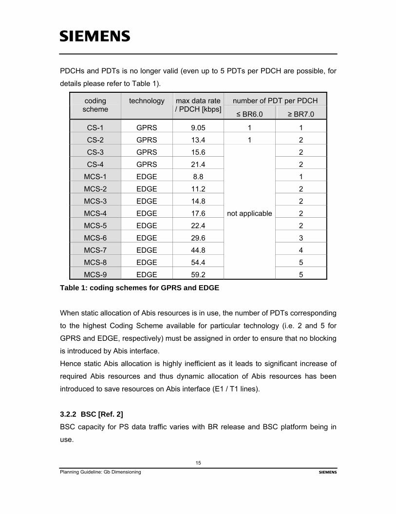
PDCHs and PDTs is no longer valid (even up to 5 PDTs per PDCH are possible, for

details please refer to Table 1).

number of PDT per PDCH coding scheme

technology max data rate / PDCH [kbps]

≤ BR6.0 ≥ BR7.0

CS-1 GPRS 9.05 1 1

CS-2 GPRS 13.4 1 2

CS-3 GPRS 15.6 2

CS-4 GPRS 21.4 2

MCS-1 EDGE 8.8 1

MCS-2 EDGE 11.2 2

MCS-3 EDGE 14.8 2

MCS-4 EDGE 17.6 2

MCS-5 EDGE 22.4 2

MCS-6 EDGE 29.6 3

MCS-7 EDGE 44.8 4

MCS-8 EDGE 54.4 5

MCS-9 EDGE 59.2

not applicable

5

Table 1: coding schemes for GPRS and EDGE

When static allocation of Abis resources is in use, the number of PDTs corresponding

to the highest Coding Scheme available for particular technology (i.e. 2 and 5 for

GPRS and EDGE, respectively) must be assigned in order to ensure that no blocking

is introduced by Abis interface.

Hence static Abis allocation is highly inefficient as it leads to significant increase of

required Abis resources and thus dynamic allocation of Abis resources has been

introduced to save resources on Abis interface (E1 / T1 lines).

3.2.2 BSC [Ref. 2] BSC capacity for PS data traffic varies with BR release and BSC platform being in

use.

s


16

Standard BSC (BSC / 46)

The PCU functionality is realized within BSC / 46 by means of PPCU boards. Each

PPCU supports up to 64 PDTs and works in cold standby (N+N) redundancy scheme

(i.e. two PPCU boards are necessary in order to configure single PCU: one of them is

in “active” state while the other one is in “standby” state and is used as spare board).

The maximum allowable GPRS configuration contains two PCUs (i.e. 4 PPCU

boards). PPCU boards can be only inserted into the same slots of BSC rack as some

PPLD boards supporting LAPD channels: in order to insert a single PPCU board 2

PPLD boards have to be removed. Every single PPLD manages up to 8 physical

LAPD channels and due to the introduction of 1 PCU (i.e. 2 PPCU boards: active and

spare) the number of PPLD boards is decreased by 4 (hence the number of LAPD

channels is decreased by 32). The overview on this effect is given by the table below:

Number of PCU per BSC Number of LAPD links per BSC

0 112

1 80

2 48

Table 2: impact of GPRS traffic on LAPD capacity for “standard” BSC

Note: Number of LAPD links per BSC refers in the table above to physical LAPD

links, both of 16 kbit/s and 64 kbit/s, either on Abis or on Asub.

Each PCU is able to handle 1 Mbit/s data flow towards the Gb interface. This amount

of PS data traffic corresponds to a flow obtained by 16 timeslots (64 kbit/s each one)

on a PCM line. These figures determine the maximum number of Frame Relay links

(PVCs) that can be configured for each PCU and the capacity expressed in terms of

bit rate. Hence for each PCU at most 16 FRLs, each one with capacity of 64 kbit/s,

can be created (max allowable capacity of a single FRL is 16 timeslots of 64 kbit/s

and it corresponds to bandwidth of 1 Mbit/s).

Standard BSC only supports GPRS CS-1 and CS-2 (and standard PCU frames).

Beginning from BR8.0 the BSC / 46 is no longer supported.

s


17

Please note that throughout the document the terms “FRL” and “PVC” are used

interchangeably. This is not a contradiction with DB planning where the following

relations are valid:

- physical channel over the Gb interface between the BSC and the SGSN is

represented by the FRL object,

- end-to-end permanent virtual connection between the BSC and the SGSN is

represented by the NSVC object,

- FRL and NSVC are associated by means of NSVLI attribute of NSVC.

For details about Gb interface related objects, attributes and interdependencies

between them please refer to the BSC Command Manual.

High Capacity BSC step I (BSC / 72)

BSC / 72 was introduced in BR6.0. The PCU functionality is realized within BSC / 72

by means of PPXU boards. Up to 6 PPXUs can be deployed within BSC / 72 and

each one supports up to 256 PDTs. Load sharing is used as redundancy scheme for

PPXUs (i.e. initially PS data traffic is dynamically distributed among all available

PPXUs; when any PPXU breaks down, PS data traffic is automatically redistributed

among the remaining PPXUs if any capacity is available). Therefore when a failure of

a PPXU occurs, then the BSC capacity expressed in terms of managed PDTs is

reduced to 1280 (i.e. 5 × 256).

Each PCU is able to handle 4 Mbit/s data flow towards the Gb interface. This amount

of PS data traffic corresponds to a flow obtained by 63 time slots (64 kbit/s each one)

on a PCM line. These figures determine the maximum number of Frame Relay links

(PVCs) that can be configured for each PCU and the capacity expressed in terms of

bit rate. Hence for each PCU at most 63 FRLs, each one with a capacity of 64 kbit/s,

can be created (max allowable capacity of a single FRL is 31 timeslots of 64 kbit/s).

High Capacity BSC supports all GPRS / EDGE Coding Schemes (as well as both

standard and concatenated PCU frames).

s


18

High Capacity BSC step II (BSC / 120)

BSC / 120 was introduced in BR7.0. The only difference between realization of PCU

functionality within BSC / 120 and BSC / 72 is capacity enhancements in number of

PPXUs managed by a BSC which is doubled from 6 in case of BSC / 72 to 12 in case

of BSC / 120 (11 when a failure of one PPXU occurs). The remaining aspects like

number of PDTs handled by a single PCU or redundancy scheme are maintained. It

simply results in a twofold increase of the capacity figures per BSC.

High speed Gb

Up to BR7.0 only Gb over Frame Relay over E1/T1 line was possible. Beginning from

BR8.0, Gb over IP over Ethernet is also available. This functionality is only

achievable with the High Capacity BSC platform. Moreover, it requires some

modification in the BSC hardware, because boards that were installed on BSCs so

far do not provide the capability of interfacing with an Ethernet switch. In order to

provide the Ethernet connectivity needed for High speed Gb interface two HW

modules (in comparison with HC BSC platform) have to be changed:

– DK40 and CPEX (in case of BSC / 72 and BSC / 120, respectively) need to be

replaced with ESAM board containing – among other things – Ethernet

switches,

– PPXUs need to be replaced with PPXUv2 (apart from functionality provided by

this board up to now a dual Ethernet port is added).

Table below gives an overview on HW modification required by the feature.

HS Gb interface HC BSC/72 HC BSC/120

ESAM DK40 CPEX

PPXUv2 PPXU PPXU

Table 3: BSC modules to be replaced due to introduction of High speed Gb-IF

Due to the introduction of the feature 'High speed Gb' some planning relevant

parameters must be updated as well. First of all, if High speed Gb is enabled, then

s


19

the PCU functionality is realized by means of PPXUv2 boards. PPXUv2 has exactly

the same capacity in terms of PDTs managed and redundancy scheme as its

predecessor but additionally it is equipped with Ethernet ports needed for external

and internal communication. Furthermore, with High speed Gb it is possible to create

up to 256 NSVCs per PCU.

Moreover, if Gb over FR over E1/T1 is in use with BR8.0, there are no differences in

the BSC capacity limitations when compared to previous releases.

The following table gives a summary on important BSC characteristics related to

GPRS:

parameter BR5.5

(BSC / 46)

BR6.0

(BSC / 72)

BR7.0

(BSC / 120)

BR8.0

(BSC / 120)

PCU

maximum number of

PCUs per BSC

2 (active) 6 12 12

PCU realisation PPCU PPXU PPXU PPXU

(PPXUv2

required for

HS Gb)

redundancy cold standby

(each active

board has its

own spare

one)

load sharing

between (up

to) 6 PPXU

boards

load sharing

between (up

to) 12 PPXU

boards

load sharing

between (up

to) 12 PPXU

boards

PDT

maximum number of

PDTs per PCU

64 256 256 256

maximum number of

PDTs per BSC

128

1536

3072

3072

s


20

parameter BR5.5

(BSC / 46)

BR6.0

(BSC / 72)

BR7.0

(BSC / 120)

BR8.0

(BSC / 120)

throughput based on PDTs

maximum throughput

per PCU

1 Mbit/s

4 Mbit/s

4 Mbit/s

4 Mbit/s

maximum throughput

per BSC

2 Mbit/s

24 Mbit/s

48 Mbit/s

48 Mbit/s

PVC

maximum number of

PVCs per PCU

16 63 63 63

(256 for

HS Gb)

maximum number of

PVCs per BSC

32 378 756 756

(3072 for

HS Gb)

Table 4: overview on important BSC parameters related to GPRS

Note that figures in brackets reported in column “BR8.0” correspond to and are only

valid for High speed (HS) Gb.

3.2.3 Physical configuration of Gb

3.2.3.1 Gb over Frame Relay Gb over FR is available in every release where GPRS / EDGE can be enabled. The

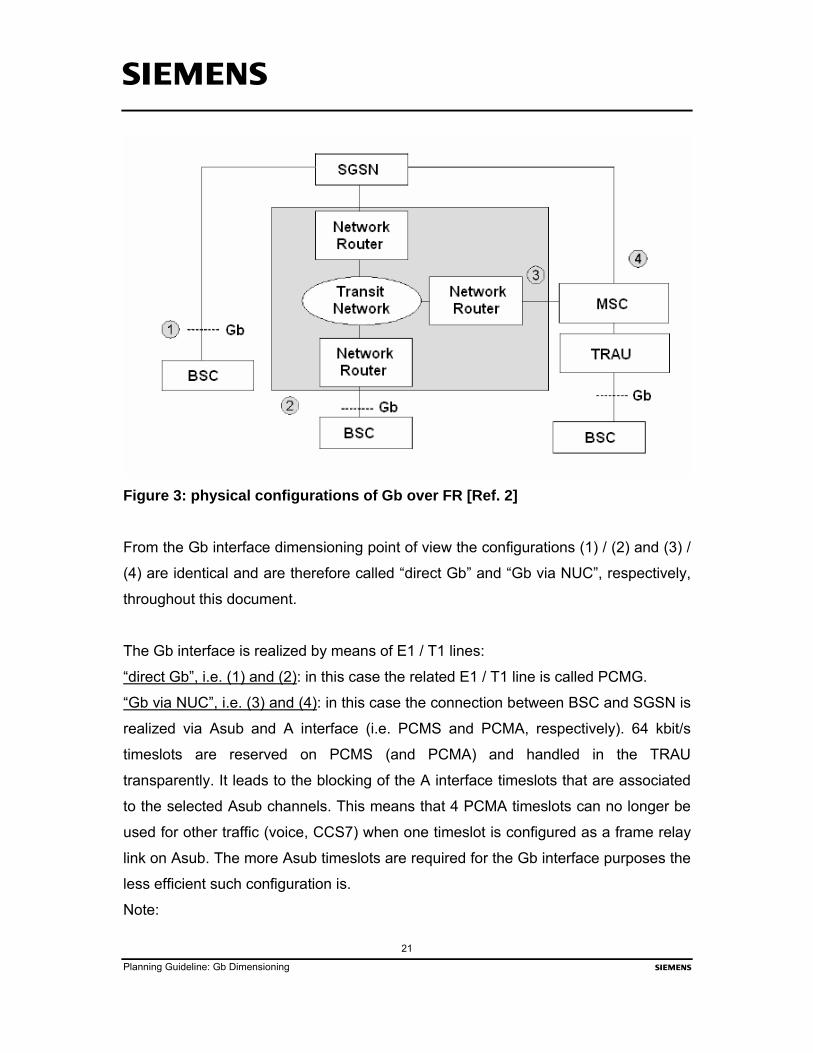
following types of configurations are possible in case of Gb over FR:

- (1) a direct line (E1 or T1) between BSC (PCU) and SGSN,

- (2) an intermediate frame relay network,

- (3) Nailed Up Connection (NUC) through the MSC via a frame relay network,

- (4) NUC through the MSC, without using an intermediate frame relay network.

These configurations are depicted in the figure below:

s


21

Figure 3: physical configurations of Gb over FR [Ref. 2]

From the Gb interface dimensioning point of view the configurations (1) / (2) and (3) /

(4) are identical and are therefore called “direct Gb” and “Gb via NUC”, respectively,

throughout this document.

The Gb interface is realized by means of E1 / T1 lines:

“direct Gb”, i.e. (1) and (2): in this case the related E1 / T1 line is called PCMG.

“Gb via NUC”, i.e. (3) and (4): in this case the connection between BSC and SGSN is

realized via Asub and A interface (i.e. PCMS and PCMA, respectively). 64 kbit/s

timeslots are reserved on PCMS (and PCMA) and handled in the TRAU

transparently. It leads to the blocking of the A interface timeslots that are associated

to the selected Asub channels. This means that 4 PCMA timeslots can no longer be

used for other traffic (voice, CCS7) when one timeslot is configured as a frame relay

link on Asub. The more Asub timeslots are required for the Gb interface purposes the

less efficient such configuration is.

Note:

s


22

In case of a multi-slot links, the MSC has to support a bit-synchronized switching of

timeslots. Otherwise links comprising more than 1 timeslot may be corrupted due to

different delays applied to the particular timeslots.

The Siemens MSC allows routing only single-slot links through its switching network

and thus it is assumed throughout this document that only single-slot links can be

configured.

Therefore a NUC configuration will cause additional delay at SGSN. Due to lower

bearer rate (i.e. 64 kbit/s in maximum) the per-hop-delay will increase significantly.

PCM lines used to realize Gb interface offer the following transmission capacities:

- E1: consists of 32 channels of 64 kbit/s equivalent to ~2 Mbit/s per line

- T1: consists of 24 channels of 64 kbit/s equivalent to ~1.5 Mbit/s per line

In both systems, one channel is used for synchronization, so 31 and 23 timeslots are

left for traffic handling for E1 and T1 lines, respectively. These resources can be

utilized by Gb interface in one out of three predefined modes: unchannelized,

channelized or fractional.

Unchannelized mode: the entire line is considered as a single channel.

3 0

2 9

2 8

2 7

17

16

15

12

11

10 9 8 7 6 5 4 3 2 1 03

1

Unchannelized ("1 stream ") TS 31

Figure 4: unchannelized mode

Channelized mode: a single line contains several channels. They are formed from the

necessary number of timeslots, which are not necessarily consecutive.

3 0

2 9

2 8

2 7

2 4

23

22

17

16

15

12

11

10 9 8 7 6 5 4 3 2 1 03

1

Channelized ( groups single timeslots together )

stream 1 stream 2 Figure 5: channelized mode

s


23

Fractional mode: only part of a line comprises a channel. The remaining timeslots are

left idle.

3 0

2 9

2 8

2 7

2 4

23

22

17

16

15

12

11

10 9 8 7 6 5 4 3 2 1 03

1

Fractional (1 stream , defined number of timeslots )

Figure 6: fractional mode

The bandwidth that can be assigned to a single frame relay link depends on Gb

physical realization and is expressed in terms of TSs that can be used to configure a

FRL. The table below gives a summary:

PCM system direct Gb Gb via NUC

E1 ≥ 1 and ≤ 31 1

T1 ≥ 1 and ≤ 23 1

Table 5: number of TSs available per FRL

As it can be seen in the table above the capacity of frame relay link is limited by the

PCM line bandwidth in case of “direct Gb” and MSC capabilities for “Gb via NUC”.

Obviously, if a higher bandwidth than the one offered by a single frame relay link is

required by a PCU, then additional links (PVCs) must be created.

3.2.3.2 Gb over IP Before BR8.0, the Gb interface was only handled over a Frame Relay network.

Beginning from BR8.0 also Gb over IP is possible. The functionality called “High

speed Gb” utilizes IPv4 over either Fast Ethernet offering 100 Mbps or over Gigabit

Ethernet both with IEEE 802 or Ethernet II.

The introduction of Ethernet causes that a distance of up to 100 m between the BSC

Ethernet Switch and the SGSN or a router to a WAN interface must be kept. The

overall network view is shown in the figure below:

s


24

Figure 7: High speed Gb interface connected to the SGSN by means of a router

This limited transmission range is surely sufficient if the BSC and the SGSN are co-

located. Otherwise the operator has to ensure that the first router of the IP Network

used for Gb is located within the Ethernet distance from the BSC. This router will then

provide the WAN interfaces needed for extension the distance to the SGSN site / IP

network. Such configuration enables the WAN interface to be selected according to

the traffic volume and almost independent of the interface options offered by BSC

and SGSN suppliers. The interfaces used in the external network (i.e. beyond the

External Router from the BSC’s perspective) are out of scope of Gb interface

dimensioning.

This feature can be supported by High Capacity BSC platform after small

modifications of its HW (for details related to BSC architecture please refer to 3.2.2).

3.2.4 Redundancy aspects Redundancy is needed to prevent or alleviate consequences of failures. In

connection with Gb interface dimensioning at least redundancy of:

- PCU board,

- E1/T1 or Ethernet links between BSC and SGSN

must be ensured.

s


25

The redundancy scheme of PCU board depends on BSC platform being in use. In

particular cold standby and load sharing techniques are exploited in Standard BSC

and High Capacity BSC, respectively.

In case of cold standby every single PCU has its own spare board available in BSC.

When failure of an active PCU occurs then its whole traffic is completely taken over

by the redundant board.

In case of load sharing the entire traffic is distributed among all PCUs the BSC is

equipped with. When failure of a PCU occurs then the traffic is re-distributed among

the remaining PCUs. Hence, in order to ensure redundancy, a spare PCU must be

added in addition to the number of active PCUs computed by means of eq. (32).

The link redundancy concept consists in having transmission links not fully loaded,

e.g. with 2 E1 links loaded at 50% it is possible to overcome a failure of an E1 line

without any loss of traffic and service quality.

Note:

The redundancy aspects of other links and nodes (e.g. BTS, SGSN, etc.) are out of

the scope of the document.

s


26

4 Dimensioning theory

4.1 Basic Information There are two types of wireless data transmission, i.e. Circuit Switched (CS) and

Packet Switched (PS). A CS connection is characterized by the reservation of a fixed

bandwidth which is guaranteed for the whole duration of the connection for the

specific subscriber. This characteristic makes dimensioning of CS traffic-based

networks relatively easy, because a limited number of applications is in use, these

applications are always mapped to predefined bearers, the establishment of a new

connection (both connection set-up and release are necessary) practically does not

affect already existing ones and, if no resources are available, then call attempt is

simply blocked. Unfortunately, these properties are not valid for PS connections.

Packets transmitted over PS traffic-based networks are message entities of different

lengths, which contain the information about destination and the length of packet

itself in a header. Thus the PS network is never aware of a single connection.

Particular packets are buffered and are sent, when free resources are available, to

the next hop. There, the content of header is analyzed in order to evaluate to which

destination the packet shall be routed. Furthermore, plenty of applications exist

having different requirements for bearers, packet lengths and QoS parameters.

Therefore, the well known approach based on Erlang’s first formula (Erlang B) used

for CS networks is not applicable in case of PS networks.

In order to overcome this difficulty various applications are modeled by means of

traffic descriptions. Due to very different types of QoS requirements two models are

used to describe application aggregates: elastic traffic and stream traffic.

- Elastic traffic is non real-time traffic that can cope with a non-guaranteed,

variable bandwidth but requires reliable packet delivery. Every object (e.g. a

file, a request, a transaction) needs to be transferred, and in case of packet

losses, the respective packets are retransmitted. Packet delay and delay

variation are rather unimportant, as long as the total amount of data is

delivered within a certain amount of time. Applications described by this model

are e.g. e-mail, www but also WAP and SMS.

s


27

- Stream traffic is the traffic that requires a certain bandwidth to be guaranteed.

It is (almost) real-time traffic, where the time integrity must be preserved by the

network (packet delay and delay variation are the most important quality

measures). Typical applications described by this model are e.g. VoIP, video

conferencing and video streaming.

The model determines the dimensioning method for given application.

The QoS requirements for an application are described by a traffic class. Traffic

classes are also mapped into traffic description. The main aspects that determine this

mapping are:

- QoS requirements: Conversational and streaming classes must guarantee

absolute delay and bandwidth requirements. With interactive and background

classes only 'best effort' can be achieved (and background is the least “delay

sensitive” class).

- The transport protocol: TCP or UDP are possible. TCP guarantees the

integrity of data transfers (whereas UDP does not) because it employs

feedback control mechanism to adapt the transfer rate to current network

conditions, thus, allowing flows on one link to share the available capacity.

The following table gives an overview on important applications, on traffic description

used to model these applications, on traffic classes and on transport protocols:

application www, ftp, e-mail, WAP, SMS voice, video

traffic description elastic stream

traffic classes interactive, background conversational, streaming

transport protocol TCP / UDP UDP

Table 6: traffic differentiation in GPRS networks

4.2 Queuing models

4.2.1 Kendall’s notation There is a standard notation for classifying queuing systems into different types. It

was proposed by D. G. Kendall.

s


28

In Kendall’s notation a term A/B/s-d denotes a queue with the following

characteristics:

- A denotes the probability distribution of the inter-arrival times of customers

(i.e. files to be transferred).

- B denotes the probability distribution of the service times.

- s denotes the number of service stations.

- d denotes the queuing discipline. A and B can take any of the following distribution types:

- M: exponential (Markovian) distribution,

- D: deterministic distribution,

- Ek: Erlang distribution (k denotes shape parameter),

- G: general distribution

The most frequently used queuing disciplines are:

- FIFO (FCFS): first in first out (first came first served),

- LIFO (LCLS): last in last out (last came last served),

- PS: processor sharing, i.e. all customers in the queue are processed at the

same time with a fair share.

Note: Kendall’s notation is often generalized, e.g. queuing discipline is omitted. In

such case it requires additional explanations, but usually if no queuing discipline is

specified then FIFO discipline is assumed (this assumption is also valid throughout

the document).

From the Gb dimensioning perspective, queuing models are used to evaluate which

link capacity is required on the interface to ensure that the corresponding mean

sojourn time will not exceed certain predefined threshold. The mean sojourn time is

understood as mean time needed by the system to transfer file of a given size

(length).

s


29

4.2.2 M/G/R-PS model This model can be used to describe behaviour of the queuing system where all

resources are shared equally among active flows. And this is the case when the

control loop of the TCP transport protocol is in use. With this model an end-to-end

delay is derived (in contrast to the M/M/1 model – which calculates a per-hop delay).

At the Gb-IF normally there is a maximum transmission rate for each connection

(rpeak) due to the limited transmission rate at the air interface. In such case the ratio

between the link capacity C and the peak data rate per subscriber rpeak represents the

number of servers R in the processor sharing queue or the number of connections

that can be served in parallel, respectively:

(1) ⎥⎥⎦

⎥

⎢⎢⎣

⎢=

peakrCR

Here we can say that the totally available bandwidth (the link capacity C) is split into

R pieces each with a bandwidth of rpeak, hence up to R “pieces” can be served at the

same time without any rate reduction being imposed by the system.

For the M/G/R-PS model, the expected sojourn time ( ){ }xTE for a file of size x is

given by:

(2) ( ){ } ( ) peak

2

rx

1RE1xTE ⋅⎟⎟

⎠

⎞⎜⎜⎝

⎛ρ−

+=

with the utilization rate ρ

(3) Cxmeane ⋅λ

=ρ

where eλ and xmean stand for the mean arrival rate of elastic traffic calls and mean file

size, respectively. E2 represents Erlang’s second formula (Erlang C formula) and can

be computed as:

(4) ( ) ( ) 12

122 VV1

VR,REE+ρ−

=ρ=

(5) ( ) ( )∑−≤

ρ⋅=ρ⋅=1Ri

i

2

R

1 !iRV,

!RRV

s


30

Note that expression ( )⎟⎟⎠⎞

⎜⎜⎝

⎛ρ−

+=1RE1f 2

R is often called “delay factor” as it represents

the increase of the mean transfer time imposed by the system (denoted by the factor

of x / rpeak).

Theoretically the M/G/R-PS model can be also specialized for R = 1 which leads to

the M/G/1-PS model. It can be used if the peak data rate a subscriber can get in a

cell (rpeak) is higher than the link capacity C. This happens rarely on the Gb interface.

Nevertheless, for the sake of completeness, with rpeak = C and R = 1 the expected

sojourn time ( ){ }xTE is

(6) ( ){ }Cx

11xTE ⋅

ρ−=

4.2.3 M/M/1 model This model assumes that the whole information can be transferred by a single packet

with a packet length of x (file length = packet length). With this model a per-hop delay

is derived only (in contrast to the M/G/R-PS where end-to-end delay is derived). In

this case, the expected sojourn time ( ){ }xTE for a file of size x is given by:

(7) ( ){ }Cx

11xTE ⋅

ρ−=

With the sojourn time it is possible to derive the required capacity C. It can be

computed as follows:

(8) meanemean xT

xC ⋅λ+=

where T, eλ and xmean stand for the mean transfer time, the mean arrival rate of

elastic traffic calls and the mean file size, respectively.

4.2.4 Dimensioning model for stream traffic Both M/G/R-PS and M/M/1 models are applicable for elastic traffic (for details please

refer to chapter 4.3.1). However they can not be used to describe stream traffic

properly. Instead, although stream is PS data traffic, the most appropriate way to

model stream traffic is a voice call. In order to perform the dimensioning of stream

s


31

traffic, firstly, the particular service classes (needed to carry requested applications)

must be recognized and described with the following characteristics:

- a homogeneous traffic pattern, i.e.

o effective bandwidth required by application,

o the amount of traffic that can / must be offered for given application,

- a common QoS profile, i.e. maximum acceptable blocking rate.

Below the characteristics of the service classes are described:

Effective bandwidth quantifies the impact of a new call (session) on the network. It

depends on many different factors (e.g. application characteristics, network topology

…) and there is no analytical formula to derive the exact value in advance. However,

for a rough estimation, the effective bandwidth can be derived from the guaranteed

and the peak bit rate (which are stream traffic relevant parameters that are negotiable

by the user) by means of the following formula:

(9) ( ) ( ) ( ) ( )( )iGipeakiGi rrfre −⋅+=

where: e(i) – effective bandwidth for service class i,

rG(i) – guaranteed bit rate for service class i,

rpeak(i) – peak bit rate for service class i,

f ∈ [0;1].

Note:

Until further information is available it is suggested to use a factor f in the range of

0.25 to 0.5. Higher values can be selected for more conservative dimensioning.

Offered traffic (also called offered load) can be computed by means of the following

formula:

(10) )i(

)i()i()i(1ea

µ⋅λ⋅=

where: a(i) – offered load for service class i,

λ(i) – arrival intensity per time unit for service class i,

µ(i) – mean service time for service class i.

s


32

Note that stream traffic which is offered by the radio interface is usually expressed in

terms of Erlangs. In such cases the formula above can be modified as follows:

(11) )i()i()i( Aea ⋅=

where A(i) means offered Erlang traffic per class i.

Blocking probability can be reasonably chosen from the range of 1% to 0.1% (even

less blocking rates can be selected for more conservative dimensioning). Of course,

when information about blocking rate required by particular application is available, it

shall be applied.

When the characteristics described above, i.e.:

- effective bandwidth e(i),

- offered traffic a(i),

- required blocking rate B(i)

are defined for each service class, the stream traffic can be dimensioned by means

of the multidimensional Erlang (MDE) formula.

4.3 Dimensioning rules for different traffic descriptions

4.3.1 Models’ applicability Different applications described by elastic traffic have various distributions of the file

arrival processes and service times. However, for Gb interface dimensioning

purposes, differentiation between TCP and UDP traffic aggregates is done rather

than between applications themselves. Therefore three traffic types are to be

distinguished as far as elastic traffic is to be concerned:

- TCP

- UDP

- mixture of TCP and UDP.

Most of the currently used applications exploit the TCP transport protocol as their

mean packet lengths are significantly shorter than their mean file lengths. For

instance www, ftp and e-mail are examples of TCP-based elastic applications. The

s


33

UDP transport protocol is relevant for applications having the file size in the order of

the packet size, e.g. WAP, SMS and MMS.

Links where pure TCP and UDP traffic is present shall be dimensioned by means of

M/G/R-PS and M/M/1 models, respectively.

In case of stream traffic a demanding application can be more critical from the Gb

interface perspective. Therefore the multidimensional Erlang B formula or the model

described in the chapter 4.2.4 shall be used.

4.3.2 Dimensioning targets Due to their different nature elastic traffic and stream traffic have different

dimensioning targets to be fulfilled.

For elastic traffic it is important to ensure that a transfer of a file of a given length lf

(e.g. the size of web page) must be finished within a certain time t (e.g. the time a

user tolerates to wait for a download of a web page). Unfortunately, as long as no

admission control is in use, it is not possible to guarantee a required time for a single

file transfer. Therefore a certain mean delay (Td,mean) shall be guaranteed for a certain

mean file length (lf,mean).

For stream traffic a certain transmission time (i.e. delay) for given session can not be

considered as dimensioning target to be reached. If the required parameters are not

met, the QoS for all ongoing stream traffic will be lost (and the service suspends, i.e.

it fails if real time service is utilized). Therefore, as for CS services, user perceptible

QoS parameters can only be defined by the blocking rates for particular service

classes.

4.3.3 Dimensioning rules for TCP For a given offered elastic traffic (rav,PVC), the peak throughput rate achievable by

subscriber in a cell (rpeak) and a delay factor (fR > 1), the required link capacity

( IPDL,PVCC ) must be computed. Dimensioning is done by means of equation (2):

(12) peak

mean,fRmean,d r

lfT ⋅=

s


34

Please note that with the eq. (2) it is possible to evaluate the expected sojourn time

E{T(x)} for a transfer of file of length x. However, for dimensioning purposes, we must

rely on mean file length (lf,mean) and therefore what we can obtain from eq. (2) is

average transfer time (also called ‘total mean delay’ or ‘mean sojourn time’).

The mean file length (lf,mean) is application specific, so it can vary significantly for

different applications. However, for TCP-based applications, typically a mean file

length of 12,000 bytes is assumed.

The peak throughput rate achievable by a subscriber in a cell (rpeak) is restricted by

the performance of the air interface and therefore shall be determined during radio

planning.

It is recommended to use delay factor (fR) in the range of 5 – 10% (i.e. fR= 1.05...1.1).

The delay factor of the M/G/R-PS model (for details please refer to chapter 4.2.2) can

be evaluated by means of the equation below:

(13) ( )( )ρ−

ρ+=

1RR,RE1f 2

R

where the number of servers (R) and respective utilization rate of link (ρ) depend on

the initial link capacity ( )IPDL,PVCC as follows:

(14) ⎥⎥⎦

⎥

⎢⎢⎣

⎢=

peak

IPDL,PVC

rC

R

(15) IPDL,PVC

PVC,av

Cr

=ρ

The function E2(R, Rρ) is Erlang’s second formula and it was defined in chapter 4.2.2

(please refer to equations (4) and (5)).

A maximum PVC utilisation rate (ρ) of 70 % to 80 % is recommended in general. This

spare is mainly necessary due to the fact that the dimensioning relies on a lot of

assumptions on the amount of input traffic. For instance, incomplete descriptions of

the subscribers’ behaviour and their requirements as well as availability of huge

amount of mixed applications are reasons for existence of uncertainties in the

modelling of traffic to be transmitted over Gb.

s


35

Due to the fact that the relation between IPDL,PVCC , PVC,avr and peakr is non-linear and

non-continuous, the derivation of closed formula for IPDL,PVCC is not possible.

Therefore, starting from initial value of IPDL,PVCC , equations (13) – (15) must be

repeated iteratively until the desired mean sojourn time (Td,mean) is reached. It can be

efficiently done using procedure below:

Step 1: Choose a maximum allowed utilization rate ρ for a link (e.g. 70%). It gives

initial values for link capacity max

PVC,avIPDL,PVC

rC

ρ= as well as for the number of servers R.

Step 2: Compute the delay factor Rf and check if the desired mean sojourn time

mean,dT is already reached.

Step 3: If the mean sojourn time mean,dT is not yet fulfilled, then extend the link

capacity IPDL,PVCC (or increment R) and check the mean sojourn time again.

4.3.4 Dimensioning rules for UDP

For a offered elastic traffic rav,PVC, the link capacity IPDL,PVCC required to transfer a file of

average length of lf,mean in time of TGb must be computed. Time TGb shall be defined

as a dimensioning target. It should be at most 5-10% higher than the total required

response time for the respective service.

Dimensioning is done by means of equation (8):

(16) PVC,avGb

mean,fIPDL,PVC r

Tl

C +=

As mentioned above, the mean file length (lf,mean) is application specific and it varies

significantly with different applications. For UDP-based applications, where the

packet length is in the order of file length (the whole information is to be transferred in

one packet), typically a mean file length of 300 bytes is assumed.

Concerning a PVC utilization rate, a similar consideration as the one carried out for

TCP-based application is valid. Hence a maximum PVC utilisation rate (ρ) of 70 % to

80 % is recommended also in case of UDP traffic. Please note that it is possible to

s


36

verify whether a link with the capacity computed by means of eq. (16) also meets the

requirement on utilization rate. This can be done by means of the formula below:

(17) IPDL,PVC

PVC,av

Cr

=ρ

The eq. (16) shall be used only in case of a link carrying pure UDP traffic. Unless

very special requirements are specified there is no pure UDP traffic on the Gb

interface, while the most frequent case is a link carrying a mixture of TCP and UDP

traffic (for details please refer to chapter 4.3.5.3).

4.3.5 Dimensioning rules for mixed TCP and UDP traffic The dimensioning rules given in the last chapters are verified for traffic generated by

sources with a homogenous statistical traffic pattern on a single link. So the assumed

traffic belongs to one specific traffic class and does not interact with other traffic. This

implies the following assumption:

• In case of TCP the parameter rpeak is the same for all applications.

• In case of UDP there is a common unique mean file length lf,mean for all

applications.

Until other verified methods are available the following approaches are suggested to

handle mixed traffic class scenarios that violate the properties listed above.

4.3.5.1 Mixture of pure TCP traffic When applications with different rate limits (i.e. different values of rpeak) are present in

a single link the mean sojourn time still can be evaluated by means of equation (12).

In such case the maximum of all peak rates can be used for dimensioning purposes.

This is the worst case approach.

4.3.5.2 Mixture of pure UDP traffic When applications with different mean file lengths are present in a single link then the

equation (16) shall be modified. Assuming that there are N applications with an

offered elastic traffic rav,PVC(i), a file length of lf,mean(i) and a target transfer time of TGb(i),

the resulting link capacity can be evaluated by means of the formula below:

s


37

(18) ∑≤

+⎟⎟⎠

⎞⎜⎜⎝

⎛=

Ni)i(PVC,av

)i(Gb

)i(mean,fIPDL,PVC r

Tl

maxC

4.3.5.3 Mixture of TCP and UDP traffic If TCP and UDP traffic is present on a single link and not protected against each

other the formulas given in chapters 4.3.3 and 4.3.4 are not valid anymore. The table

below gives an overview on the recommended dimensioning methods in case of

mixed traffic depending on the Gb interface configuration.

Gb interface configuration approach

Gb via NUC Method 1

Gb over Frame Relay over E1/T1 Method 2

Gb over IP over Ethernet Method 2

Table 7: recommended dimensioning methods for mixed TCP / UDP traffic

Method 1: The link capacities for TCP and UDP traffic are computed separately. The

resulting required link capacity is the sum of the TCP and UDP bandwidths.

Method 2: The UDP traffic is regarded as TCP traffic. The resulting link capacity is

computed according to the methods given for pure TCP traffic. This is the worst case

method and will lead to significant over-dimensioning if applied to high UDP

percentages (e.g. greater than 30%).

4.3.6 Dimensioning rules for stream traffic The model described in the chapter 4.2.4 leads to the following procedure applicable

for stream traffic:

Step 1: For each (stream) traffic class an amount of traffic offered by the radio

interface and quality indicators (guaranteed and peak bit rates as well as required

blocking rate) must be known (specified). Then for i-th traffic class:

- the effective bandwidth e(i) (by means of equation (9)) and

- the offered load a(i) (by means of equation (10) or (11), depending on what

parameters are available)

s


38

must be determined.

Step 2: Dimensioning targets (i.e. required blocking rates) must be determined for

each traffic class (see chapter 4.2.4 for more information about B(i)).

Step 3: Starting with

(19) aC =

the blocking probabilities for each traffic class (for a fixed link capacity C ) are

computed by means of the multidimensional Erlang theory. C must be increased until

the blocking probabilities B(i) for each class are fulfilled. The total offered load a can

be computed by means of following formula:

(20) ∑ ∑ ⎟⎟⎠

⎞⎜⎜⎝

⎛

µ⋅λ⋅==

i i )i()i()i()i(

1eaa

4.4 Overhead factor computation In order to consider the overhead (OH) of the GPRS protocol stack the bandwidths

calculated in the chapter 4.3 have to be multiplied by an appropriate factor. This

factor is referred to as “overhead factor” (OHGb) and it is defined below:

(21) p

pGb l

ohlOH

+=

where: lp – packet length (in bytes)

oh – total overhead length for given protocol stack (in bytes)

Both elements of the equation below can be computed based on the information

provided in the forthcoming chapters.

4.4.1 Total overhead length The total overhead length (oh) depends on the size of the headers of the protocols

being part of the GPRS protocol stack. As mentioned above (general information

about the GPRS protocol stack for Gb is given in the chapter 3.1) the protocol stack

s


39

at the Gb interface is SNDCP over LLC over BSSGP over some Network Service

transport. Depending on realization of Gb interface the NS transport can be based:

- either on Frame Relay

- or on IP over Ethernet.

Therefore the total overhead length (oh) must be evaluated for these two different

cases. Nevertheless, the contribution of the highest Gb interface specific layers

(SNDCP, LLC, BSSGP and NS) is constant and the worst case lengths of their

headers are depicted in the figure below:

Figure 8: Gb interface specific protocol layers and lengths of their headers

Hence the overheads related to a particular protocols building Gb interface protocol

stack are outlined below:

(22)

4oh53oh

40oh4oh

NS

BSSGP

LLC

SNDCP

==

==

The remaining overheads (related to “Layer 2 Protocols” part of Gb header) must be

considered according to the chosen realization of Gb interface. Lengths of overhead

corresponding to Gb over Frame Relay and Gb over IP over Ethernet are reported in

the chapters 4.4.1.1 and 4.4.1.2, respectively.

s


40

4.4.1.1 Frame Relay In case of Gb over Frame Relay over E1 / T1 the sub-network service is ensured by

Frame Relay protocol. The FR header is the one with a length of 8 bytes. Six bytes

are from the Q.922 overhead and two bytes are from the RFC 1490 header. Thus, for

further calculation purposes the following formula can be used:

(23) 8ohFR =

The header format is shown in the figure below:

Figure 9: overhead Frame Relay

4.4.1.2 IP over Ethernet In case of Gb over IP over Ethernet the sub-network service is ensured by IP over

Ethernet. The Ethernet header is the one with a length of 34 bytes. Twenty six bytes

are from the Ethernet (IEEE802.3) overhead and eight bytes are from the LLC /

SNAP (IEEE802.2) overhead. Thus, for further calculation purposes the following

formula can be used:

(24) 34ohEth =


s


41

Figure 10: overhead Ethernet

If Gb interface is realized over Ethernet then UDP and IP protocols are used at

transport level (in the protocol stack the following sequence occurs: …, NS, UDP, IP,

Ethernet).

The UDP header is the one with a length of 8 bytes. Thus, for further calculation

purposes the following formula can be used:

(25) 8ohUDP =


Figure 11: overhead UDP

The IP header is the one with a length between of 20 and 24 bytes. As shown in the

figure below 4 bytes of the header are optional and usually are not taken into

consideration in calculations. Thus, for further calculation purposes the following

formula can be used:

(26) 20ohIP =

s


42


Figure 12: overhead IP

4.4.1.3 Total overhead lengths on Gb interface

Based on equations (22) – (26) the total overhead lengths FRoh and IPoEthoh can be

computed for Gb over Frame Relay and Gb over IP over Ethernet, respectively. The

following formulae can be used for further calculations:

Total overhead length for Gb over Frame Relay:

(27) 109ohohohohohoh FRNSBSSGPLLCSNDCPFRoPCM =++++=

Total overhead length for Gb over IP over Ethernet:

(28) 163ohohohohohohohoh EthIPUDPNSBSSGPLLCSNDCPIPoEth =++++++=

4.4.2 Packet length The overhead factor depends on the packet lengths as defined in the equation (21).

Typical packet lengths are given in the table below:

TCP UDP

lengths (bytes) lengths (bytes)

UL packet length (Ip,UL) 80 44

s


43

TCP UDP

lengths (bytes) lengths (bytes)

DL packet length (Ip,DL) • 552

• 576

• 1,500

300

Table 8: typical packet lengths

Note that besides the impact of packet lengths on overhead factors and thus on the

bandwidth to be reserved on the Gb interface, some node (e.g. SGSN) limits are

directly related to them. The performance of such devices might vary with the packet

size of files to be transferred. E.g. the number of packets to be processed within a

second is limited due to a CPU processing power. Therefore for a fixed average

bandwidth smaller packets require more resources and this will decrease the overall

node performance.

If different applications are mixed (e.g. TCP and UDP) then the packet lengths have

to be averaged in order to compute the corresponding overhead factor. The average

packet size ( tot,pl ), in case of two different applications (e.g. TCP and UDP), is given

by the following formula:

(29) ( )UDPUDP,pUDPTCP,p

UDP,pTCP,ptot,p r1lrl

lll

−⋅+⋅⋅

=

Above Ip,tot is the packet length averaged for UDP and TCP traffic. Ip,TCP is the TCP

packet length and Ip,UDP is the UDP packet length. rUDP and Ip,tot are the share of UDP

traffic and the packet length averaged for UDP and TCP traffic, respectively.

4.5 Capacity reserves When more than 1 PVC is created per PCU, then a certain capacity reserve is

recommended. This can be the case if redundancy by load sharing of 2 PVCs per

PCU is required and if the traffic must be served either by several NUCs (in case of

Gb via NUC, for details please refer to the chapter 3.2.3.1) or by several FRLs (when

the capacity required by the PCU exceeds 31 channels of 64 kbit/s). This spare

s


44

capacity is necessary because the load sharing techniques are not ideal and thus

absolutely balanced traffic on all PVCs cannot be ensured.

In case of 1 PVC per PCU no capacity reserve is needed whereas for the Gb

interface operating with load sharing the capacity reserve of 5–10 % is recommended

for possible non balanced traffic distribution. This additional capacity reserve will

extend required link capacity ( )GbPVCC as shown the chapter 5.1 (3rd step of

dimensioning procedure).

s


45

5 Dimensioning in practice Figure 13 shows a model of the traffic flows that can be transmitted over Gb

interface:

Figure 13: Logical link model

Theoretically, depending on the deployed QoS mechanisms, the model given above

has the following consequences on the Gb interface dimensioning:

- Traffic in one class can affect traffic in any other class.

- Overload in one class can affect any of the other classes.

- One class can use bandwidth shares of other classes whenever they are not

fully utilized (multiplexing gain).

However such general approach taking into account all possible configurations,

interactions and multiplexing gain is too complex for network planning purposes. To

simplify dimensioning the following assumptions were made:

- No multiplexing gains between different classes are taken into account.

- Overload situations are avoided before actual dimensioning of a link by e.g.

the worst case evaluation of the offered traffic.

The algorithms given in chapter 4.3 allow a reasonable estimation of the behaviour of

a link loaded with PS traffic. Nevertheless even with these assumptions the accuracy

of the final result strongly depends on how precise the description of the offered

traffic was.

s


46

5.1 Dimensioning steps The final goal of the Gb interface dimensioning from the BSS point of view is to

determine the required transmission capacities (e. g. the number of PCMG lines or

number of TSs needed at Asub-IF). The chart below shows the most important steps

that must be carried out in order to do Gb interface dimensioning.

Figure 14: Gb interface dimensioning steps

The activities to be done within particular steps can be described as follows:

Step 1: evaluation of BSC offered traffic

BSC offered traffic can be evaluated by means of the formula below:

(30) GPRSBSC,subsub,avBSC,av RNrr ⋅⋅=

where: rav,BSC – average throughput rate per BSC,

rav,sub – average throughput rate per data subscriber,

Nsub,BSC – number of subscribers per BSC,

RGPRS – percentage of data subscribers within the BSC.

Both elastic and stream traffic volumes must be computed as starting point for further

dimensioning steps. Particular applications have to be assigned to traffic classes

according to QoS requirements to be met (e.g. SMSs shall be assigned either to

interactive or to background class).

Depending on the realization of the Gb interface (FR over E1/T1 or IP over Ethernet)

dimensioning is done on the basis of either the traffic aggregated in the PCU or the

one aggregated in the BSC. In case of FR over E1/T1 a link is a single PVC (FRL)

whereas in case of Ethernet a physical interface must be treated as a link.

required linkCapacity

bandwidth required on the Gb

overhead

spare capacity

Elastic traffic (TCP / UDP)

offered traffic per BSC

Stream traffic

required linkCapacity

bandwidth required on the Gb

overhead

spare capacity

Elastic traffic (TCP / UDP)

offered traffic per BSC

Stream traffic

s


47

Therefore – if Frame Relay is concerned as sub-network service – after evaluation of

the traffic volume per BSC, it must be distributed between available PCUs. For

dimensioning purposes a fully homogenous distribution is assumed as shown in the

formula below:

(31) BSC,PCU

BSC,avPCU,av N

rr =

where: rav,PCU – average throughput rate per PCU,

NPCU,BSC – number of PCUs per BSC.

The number of active PCUs per BSC can be computed as follows:

(32) ⎥⎥

⎤⎢⎢

⎡=

PCU,PDT

BSC,PDTBSC,PCU N

NN

where: NPDT,BSC – the number of 16 kbit/s Abis channels dedicated for data

traffic (PDTs) per BSC

NPDT,PCU – the maximum number of PDTs per PCU. It depends on PCU

realization and the respective values for each release as outlined in the

Table 4

Furthermore, when more than 1 PVC per PCU is necessary (see chapter 4.5) it is

considered by:

(33) PCU,PVC

PCU,avPVC,av N

rr =

where: rav,PVC – average throughput rate per PVC,

NPVC,PCU – required number of PVCs per PCU.

Step 2: evaluation of the required link capacity

Calculation steps depend on traffic pattern available in the link. The following cases

are the most frequent ones:

- “pure” elastic traffic (TCP, UDP or mixture)

- “pure” stream traffic

s


48

- mixture of elastic and stream.

Therefore, first the decision shall be made which dimensioning model is applicable

and then proper algorithm(s) from among the ones described in chapter 4.3 shall be

used.

For elastic traffic, based on the configuration of Gb interface (i.e. link capacity), one

can select:

- pure TCP traffic: M/G/R-PS model

- mixture of TCP and UDP traffic, Gb via NUC: method 1 (for details please

refer to Table 7)

- mixture of TCP and UDP traffic, “direct” Gb over Frame Relay or Gb over IP

over Ethernet: method 2 (for details please refer to Table 7)

- pure UDP traffic: M/M/1 model

For dimensioning rules related to pure TCP and UDP traffic please refer to chapters

4.3.3 and 4.3.4, respectively. Methods related to a mixture of TCP and UDP traffic

are described in chapter 4.3.5.3.

For stream traffic, the procedure described in chapter 4.3.6 shall be carried out.

Please note that offered stream traffic is usually expressed in terms of Erlangs

(please compare eq. (10) and (11)).

For a mixture of elastic and stream traffic, the earliest step is to evaluate link

capacities related to pure elastic and stream traffic, respectively. For this purpose the

procedures outlined above are applicable. Then, the link capacity including elastic

and stream can be computed as:

(34) IPstream,DL,PVC

IPelastic,DL,PVC

IPstreamelastic,DL,PVC CCC +=+

where: IPelastic,DL,PVCC , IP

stream,DL,PVCC are link capacities related to elastic traffic and stream

traffic, respectively.

Here it shall be reminded again that the expression “link” has different meanings for

Gb over Frame Relay and Gb over IP over Ethernet as it denotes single PVC (FRL)

in the former case and entire Ethernet link in the latter.

Step 3: applying overhead factors and capacity reserves

s


49

Firstly IPUL,PVCC has to be derived from IP

DL,PVCC and ratio between DL and UL

bandwidths DL/ULr by means of the formula below:

(35) DL/ULIP

DL,PVCIP

UL,PVC rCC ⋅=

A typical value of DL/ULr is 1/5 or even 1/7.

Overhead factors and capacity reserves can be considered by means of the following

formulas:

(36) resDL,GbIP

DL,PVCGb

DL,PVC fOHCC ⋅⋅=

(37) resUL,GbIP

UL,PVCGb

UL,PVC fOHCC ⋅⋅=

where: GbDL,PVCC , Gb

UL,PVCC – DL and UL capacity of a PVC including overhead and

capacity reserved, respectively

DL,GbOH , UL,GbOH – overhead factors computed based on DL,pl and UL,pl ,

respectively (for typical values of DL,pl and UL,pl please refer to Table 8

resf – capacity reserve (as described in the chapter 4.5)

Please note that different lengths of overheads have to be considered for Gb over

Frame Relay and Gb over IP over Ethernet. Based on the evaluations done in

chapter 4.4.1.3 the overhead factors can be computed as follows:

Gb over FR

(38) p

pFR,Gb l

109lOH

+=

Gb over IP over Ethernet

(39) p

pIPoEth,Gb l

163lOH

+=

As already mentioned in chapter 4.5, capacity reserve (fres) of 5-10% (i.e. 1.05 – 1.1)

are necessary when multiple PVCs are required for any reason. Note that the

s


50

capacity reserve can be also considered at an earlier point of the dimensioning

process, e.g. the offered traffic can be multiplied by a respective factor. It only has a

very small impact on the final result.

Step 4: mapping of the required bandwidth into resources on the Gb interface

The amount of physical resources on the Gb interface are computed based on

bandwidth requirements on predominant direction (usually DL). Hence total link

capacity ( )GbPVCC must be determined as:

(40) ( )GbDL,PVC

GbUL,PVC

GbPVC C;CmaxC =

This value is the one that matters for all subsequent dimensioning decisions.

Similar to the evaluation of offered traffic further steps depend on the realization of

the Gb interface. In case of Gb over Frame Relay the bandwidth requirements of a

single PVC must be multiplied by the number of PVCs created within the BSC

whereas in case of Gb over IP over Ethernet the bandwidth requirements are

determined directly by total link capacity ( )GbPVCC taking into consideration also the

maximum recommended Ethernet link load.

Gb over FR

The first step is to evaluate the number of TSs required to transmit single PVC.

Since PVCs are mapped into TSs with a capacity of 64 kbit/s, the number of TSs per

PVC can be computed as:

(41) ⎥⎥

⎤⎢⎢

⎡=

64CN

GbPVC

PVC,TS

where: GbPVCC is the total link capacity expressed in terms of kbit/s

Due to the fact that the capacity of a single PVC (FRL) is limited up to 31 TSs (for E1

line, please refer to Table 5 for details), here it must be checked whether

31N PVC,TS ≤ . If so, further steps can be done as described below, otherwise another

(i.e. one more) PVC must be created within the PCU and the calculations must be

repeated beginning from eq. (33).

s


51

Next, the contributions of all PCUs must be summed up in order to evaluate how

many TSs are necessary to transmit the bandwidth related to the PS traffic

aggregated within the BSC. It can be done by means of the formula below:

(42) BSC,PCUPCU,PVCPVC,TSBSC,TS NNNN ⋅⋅=

Finally, these TSs must be mapped onto the appropriate amount of E1 (T1) lines.

The number of TSs per PCM line that can be used for Gb interface purposes is

defined in Table 5. Additionally, it must be guaranteed that a single PVC (FRL) is not

to be split into more than one E1 line, i.e. it is possible neither to configure a PVC

being composed of more than 31 TSs nor to create the one having its TSs assigned

to different E1 lines even if less than 31 TSs are to be used in total.

In case the Gb interface is realized via a NUC through the MSC (for details please

see Figure 3 and refer to configurations (3) and (4)) dimensioning is done on the

basis of equation (40). For this configuration it must be ensured that s/kbit64CGbPVC ≤

because the Siemens MSC only allows the routing of single timeslot PVCs (FRL)

through its switching network. Hence, as long as s/kbit64CGbPVC > , the number of

PVCs per PCU must be increased and the calculations must be repeated beginning

from eq. (33). The number of NUCs (i.e. TSs on Asub / A interfaces reserved for data

traffic purposes) is equal to the decisively chosen number of PVCs (i.e. the one for

which s/kbit64CGbPVC ≤ ) .

Gb over IP over Ethernet

Based on the total link capacity computed with the eq. (40) decision is made about

the capacity of the Ethernet link to be chosen. Please note it is recommended to

keep the load of Ethernet link below 70%. Therefore the following rule can be

derived:

if s/Mbit70CGbPVC < then a Fast Ethernet link can be used, otherwise a Gigabit

Ethernet link is necessary.

s


52

The table below gives an overview on the differences between dimensioning of FR-

based and IP-based Gb interface:

#step parameter Gb over FR Gb over IP

1 dimensioning based on

the traffic aggregated:

in PCU in BSC (ESAM), i.e. in

all PCUs

2 “link” denotes: a PVC (FRL) an Ethernet link

3 overhead length of: 109 bytes 163 bytes

4 “total link capacity” is

mapped to:

TSs of 64 kbps (single

PVC can not be spread

out over more than 1

PCM line)

Ethernet link (FE or GE)

Table 9: comparison of dimensioning steps in case of Gb over FR and Gb over IP

5.2 Impact of MPCU pooling on Gb interface dimensioning MPCU (Multiple PCU) pooling was introduced from BR8.0 on. The feature allows

more than one SGSN to be connected to a BSC. It is possible due to introduction of

pooling concept: each PCU is assigned to a pool, each pool is connected to one

SGSN and different pools can be connected to different SGSNs.

s


53

Figure 15: Multiple PCU pooling

Note that the feature does not ensure SGSN redundancy (it will be possible in the

next BR release).

Every single pool needs to have its own Gb interface towards the SGSN. Obviously,

a given E1 line still can be used to carry Frame Relay links associated with different

PCUs and these PCUs not necessarily need to be part of the same pool. Thus –

when multiple PCU pooling is enabled – all calculations related to Gb-IF

dimensioning (i.e. the evaluation of offered traffic per area, the number of PCUs and

finally the number of E1 lines or NUCs or Ethernet links’ capacity) must be performed

for each pool separately rather than for the BSC as a whole. Nevertheless the

dimensioning procedure itself is not affected, i.e. it contains exactly the same steps

as without the feature, the same inputs are taken into account and the same outputs

must be obtained.

gb interface dimensioning

Documents

gb dimensioning s

gb dimensioning br8

s planning guideline

physical configuration

gb interface protocol

dimensioning theory

siemens geran

general information