garbage collection for flexible hard real-time systems

Garbage Collection for Flexible Hard Real-Time

Systems

Yang Chang

Submitted for the degree of

Doctor of Philosophy

University of York

Department of Computer Science

October 2007

To Mum and Dad

Abstract

Garbage collection is key to improving the productivity and code quality in virtu-

ally every computing system with dynamic memory requirements. It dramatically

reduces the software complexity and consequently allows the programmers to con-

centrate on the real problems rather than struggling with memory management

issues, which finally results in higher productivity. The code quality is also im-

proved because the two most common memory related errors — dangling pointers

and memory leaks — can be prevented (assuming that the garbage collectors are

implemented correctly and the user programs are not malicious).

However, real-time systems, particularly those with hard real-time requirements,

always choose not to use garbage collection (or even dynamic memory) in order to

avoid the unpredictable executions of garbage collectors as well as the chances of

being blocked due to the lack of free memory. Much effort has been expended

trying to build predictable garbage collectors which can provide both temporal and

spatial guarantees. Unfortunately, most existing work leads to systems that cannot

easily achieve a balance between temporal and spatial performance, although their

worst-case behaviours in both dimensions can be predicted. Moreover, the real-time

systems targeted by the existing real-time garbage collectors are not the state-of-

the-art ones. The scheduling of those garbage collectors has not been integrated into

the modern real-time scheduling frameworks, which makes the benefits provided by

those systems very difficult to obtain.

This thesis argues that the aforementioned issues should be tackled by introduc-

ing new design criteria for real-time garbage collectors. The existing criteria are not

enough to reflect the unique requirements of real-time systems. A new performance

indicator is proposed to describe the capability of a real-time garbage collector to

achieve better balance between temporal and spatial performance. Moreover, it is

argued that new real-time garbage collectors should be integrated with the real-time

task model and more advanced scheduling techniques should be adopted as well.

A hybrid garbage collection algorithm, which combines both reference counting

and mark-sweep, is designed according to the new design criteria. On the one hand,

the reference counting component helps reduce the overall memory requirements. On

the other hand, the mark-sweep component periodically identifies cyclic garbage,

which cannot be found by the reference counting component. Both parts of the

collector are executed by segregated tasks, which are released periodically as the

hard real-time user tasks. In order to improve the performance of soft- or non-real-

time tasks in our system while still guaranteeing the hard real-time requirements,

the dual-priority scheduling algorithm is used for all the tasks including the GC

tasks. A multi-heap approach is also proposed to bound the impacts of the soft-

or non-real-time tasks on the overall memory usage as well as the executions of the

GC tasks. More importantly, static analyses are also developed to provide both

temporal and spatial guarantees for the hard real-time tasks.

The aforementioned system has been implemented and tested. A series of exper-

iments are presented and explained to prove the effectiveness of our approach. In

particular, a few synthetic task sets, including both hard and soft- or non-real-time

tasks, are analyzed and executed along with our garbage collector. The performance

of the soft- or non-real-time tasks is demonstrated as well.

Contents

1 Introduction 1

1.1 Real-Time Systems . . . . . . . . . . . . . . . . . . . . . . . . . . . . 3

1.2 Memory Management . . . . . . . . . . . . . . . . . . . . . . . . . . . 8

1.3 Research Scope . . . . . . . . . . . . . . . . . . . . . . . . . . . . . . 16

1.4 Motivation, Methodology, Hypothesis and Contributions . . . . . . . 17

1.5 Thesis Structure . . . . . . . . . . . . . . . . . . . . . . . . . . . . . . 22

2 Garbage Collection and Related Work 25

2.1 Introduction . . . . . . . . . . . . . . . . . . . . . . . . . . . . . . . . 26

2.2 Reference Counting . . . . . . . . . . . . . . . . . . . . . . . . . . . . 26

2.2.1 Deferred Reference Counting . . . . . . . . . . . . . . . . . . . 28

2.2.2 Lazy Freeing . . . . . . . . . . . . . . . . . . . . . . . . . . . . 29

2.2.3 Local Mark-Sweep . . . . . . . . . . . . . . . . . . . . . . . . 30

2.3 Basic Tracing Garbage Collection . . . . . . . . . . . . . . . . . . . . 33

2.3.1 Mark-Sweep and Mark-Compact Garbage Collection . . . . . 34

2.3.2 Copying Garbage Collection . . . . . . . . . . . . . . . . . . . 35

2.3.3 Root Scanning . . . . . . . . . . . . . . . . . . . . . . . . . . 38

2.4 Generational Garbage Collection . . . . . . . . . . . . . . . . . . . . 42

i

2.5 Incremental Garbage Collection . . . . . . . . . . . . . . . . . . . . . 46

2.5.1 Brief Review of Incremental Garbage Collection . . . . . . . . 46

2.5.2 Incremental Copying Garbage Collectors . . . . . . . . . . . . 52

2.5.3 Non-Copying Incremental Garbage Collectors . . . . . . . . . 56

2.5.4 Some Real-time Issues . . . . . . . . . . . . . . . . . . . . . . 59

2.5.5 Concurrent Garbage Collection . . . . . . . . . . . . . . . . . 65

2.6 Contaminated Garbage Collection . . . . . . . . . . . . . . . . . . . . 67

2.7 State-of-the-art Real-time Garbage Collection . . . . . . . . . . . . . 70

2.7.1 Henriksson’s Algorithm . . . . . . . . . . . . . . . . . . . . . . 71

2.7.2 Siebert’s Algorithm . . . . . . . . . . . . . . . . . . . . . . . . 73

2.7.3 Ritzau’s Reference Counting Algorithm . . . . . . . . . . . . . 76

2.7.4 Metronome Garbage Collector . . . . . . . . . . . . . . . . . . 77

2.7.5 Kim et al.’s Algorithm . . . . . . . . . . . . . . . . . . . . . . 80

2.7.6 Robertz et al.’s Algorithm . . . . . . . . . . . . . . . . . . . . 82

2.8 Summary . . . . . . . . . . . . . . . . . . . . . . . . . . . . . . . . . 83

3 New Design Criteria for Real-Time Garbage Collection 85

3.1 Problem Statements . . . . . . . . . . . . . . . . . . . . . . . . . . . 85

3.2 Decomposition of the Overall Memory Requirements and Garbage

Collection Granularity . . . . . . . . . . . . . . . . . . . . . . . . . . 90

3.3 Flexible Real-Time Scheduling . . . . . . . . . . . . . . . . . . . . . . 101

3.4 New Design Criteria . . . . . . . . . . . . . . . . . . . . . . . . . . . 105

3.5 Revisiting Existing Literature . . . . . . . . . . . . . . . . . . . . . . 109

3.5.1 Existing Real-time Garbage Collectors . . . . . . . . . . . . . 109

ii

3.5.2 Existing Non-real-time Garbage Collectors . . . . . . . . . . . 114

3.6 Summary . . . . . . . . . . . . . . . . . . . . . . . . . . . . . . . . . 117

4 Algorithm and Scheduling 119

4.1 The Hybrid Approach Overview . . . . . . . . . . . . . . . . . . . . . 119

4.2 Data Structures . . . . . . . . . . . . . . . . . . . . . . . . . . . . . . 127

4.2.1 Building Objects and Arrays with Fixed Size Blocks . . . . . . 127

4.2.2 Object Headers and Garbage Collector’s Data Structures . . . 133

4.3 Write Barriers . . . . . . . . . . . . . . . . . . . . . . . . . . . . . . . 140

4.4 Tracing, Reclamation and Allocation . . . . . . . . . . . . . . . . . . 150

4.5 Scheduling . . . . . . . . . . . . . . . . . . . . . . . . . . . . . . . . . 159

4.5.1 Making GC Tasks Periodic . . . . . . . . . . . . . . . . . . . . 159

4.5.2 Scheduling GC Tasks . . . . . . . . . . . . . . . . . . . . . . . 162

4.6 Summary . . . . . . . . . . . . . . . . . . . . . . . . . . . . . . . . . 167

5 Static Analysis 170

5.1 Notation Definition and Assumptions . . . . . . . . . . . . . . . . . . 171

5.2 The Period and Deadline of the GC Tasks . . . . . . . . . . . . . . . 174

5.3 The WCETs of the GC Tasks . . . . . . . . . . . . . . . . . . . . . . 184

5.4 Schedulability Analysis . . . . . . . . . . . . . . . . . . . . . . . . . . 189

5.5 Further Discussions . . . . . . . . . . . . . . . . . . . . . . . . . . . . 191

5.6 Summary . . . . . . . . . . . . . . . . . . . . . . . . . . . . . . . . . 197

6 Prototype Implementation and Experiments 199

6.1 Prototype Implementation . . . . . . . . . . . . . . . . . . . . . . . . 200

iii

6.1.1 Environment . . . . . . . . . . . . . . . . . . . . . . . . . . . 200

6.1.2 Memory Organization and Initialization . . . . . . . . . . . . 204

6.1.3 Limitations . . . . . . . . . . . . . . . . . . . . . . . . . . . . 206

6.2 Platform and Experiment Methodology . . . . . . . . . . . . . . . . . 207

6.3 Evaluations . . . . . . . . . . . . . . . . . . . . . . . . . . . . . . . . 209

6.3.1 Barrier Execution Time . . . . . . . . . . . . . . . . . . . . . 209

6.3.2 RR, TR and IR . . . . . . . . . . . . . . . . . . . . . . . . . 213

6.3.3 Worst-Case Blocking Time . . . . . . . . . . . . . . . . . . . . 218

6.3.4 Allocation . . . . . . . . . . . . . . . . . . . . . . . . . . . . . 221

6.3.5 Synthetic Examples . . . . . . . . . . . . . . . . . . . . . . . . 223

6.3.6 The Response Time of A Non-Real-Time Task . . . . . . . . . 240

6.4 Summary . . . . . . . . . . . . . . . . . . . . . . . . . . . . . . . . . 243

7 Relaxing the Restrictions on Soft- and Non-Real-Time Tasks 244

7.1 Algorithm and Scheduling . . . . . . . . . . . . . . . . . . . . . . . . 245

7.2 Adjusting the Previous Analysis . . . . . . . . . . . . . . . . . . . . . 257

7.3 Detecting Illegal References . . . . . . . . . . . . . . . . . . . . . . . 258

7.4 Evaluations . . . . . . . . . . . . . . . . . . . . . . . . . . . . . . . . 261

7.4.1 A Synthetic Example . . . . . . . . . . . . . . . . . . . . . . . 263

7.5 Summary . . . . . . . . . . . . . . . . . . . . . . . . . . . . . . . . . 281

8 Conclusions and Future Work 283

8.1 Meeting the Objectives . . . . . . . . . . . . . . . . . . . . . . . . . . 283

8.2 Limitations and Future Work . . . . . . . . . . . . . . . . . . . . . . 286

8.3 In Conclusion . . . . . . . . . . . . . . . . . . . . . . . . . . . . . . . 290

iv

List of Figures

2.1 How Bacon and Rajan improved Lins’ algorithm . . . . . . . . . . . . 33

2.2 Copying collection . . . . . . . . . . . . . . . . . . . . . . . . . . . . 37

2.3 Weak tri-colour invariant: unsuitable for copying algorithms . . . . . 49

2.4 Baker’s incremental copying algorithm . . . . . . . . . . . . . . . . . 53

2.5 Treadmill GC algorithm . . . . . . . . . . . . . . . . . . . . . . . . . 58

4.1 An object’s memory layout . . . . . . . . . . . . . . . . . . . . . . . . 129

4.2 The problem with compacting an object . . . . . . . . . . . . . . . . 130

4.3 An array structure . . . . . . . . . . . . . . . . . . . . . . . . . . . . 131

4.4 The pseudocode of array field access operations . . . . . . . . . . . . 131

4.5 Increasing the block size does not necessarily increase the amount of

wasted memory . . . . . . . . . . . . . . . . . . . . . . . . . . . . . . 132

4.6 Data structures . . . . . . . . . . . . . . . . . . . . . . . . . . . . . . 136

4.7 The memory layout of an object header . . . . . . . . . . . . . . . . . 139

4.8 The pseudocode of write barrier for objects . . . . . . . . . . . . . . . 142

4.9 The pseudocode of write barrier for roots . . . . . . . . . . . . . . . . 143

4.10 The pseudocode of write barrier for prologue . . . . . . . . . . . . . . 146

4.11 The pseudocode of write barrier for epilogue . . . . . . . . . . . . . . 147

v

4.12 The pseudocode of write barrier for objects after return . . . . . . . . 149

4.13 The pseudocode of the reclaiming task . . . . . . . . . . . . . . . . . 154

4.14 The pseudocode of the tracing task . . . . . . . . . . . . . . . . . . . 156

4.15 The pseudocode of the object allocator . . . . . . . . . . . . . . . . . 158

5.1 The number of releases of a user task during a GC period . . . . . . . 181

5.2 Determining the priorities of the GC tasks . . . . . . . . . . . . . . . 185

5.3 The extra interference from the GC tasks . . . . . . . . . . . . . . . . 191

6.1 The structure of the prototype implementation . . . . . . . . . . . . . 201

6.2 The WCET estimations of write barriers . . . . . . . . . . . . . . . . 213

6.3 The WCET estimations of block reclamation . . . . . . . . . . . . . . 215

6.4 The WCET estimations of block tracing . . . . . . . . . . . . . . . . 217

6.5 The WCET estimations of tracing initialization . . . . . . . . . . . . 218

6.6 The relation between the worst-case blocking time introduced by the

allocator and the number of blocks that are to be processed as a group221

6.7 The relation between the computation time of the allocator and the

requested memory size . . . . . . . . . . . . . . . . . . . . . . . . . . 222

6.8 Task set 1 with promotion delay 0ms . . . . . . . . . . . . . . . . . . 233

6.9 Task set 1 with promotion delay 10ms . . . . . . . . . . . . . . . . . 233





6.14 Task set 2 with promotion delay 0ms . . . . . . . . . . . . . . . . . . 236

vi






6.20 Response time of a non-real-time task (iteration A) with different GC

promotion delays . . . . . . . . . . . . . . . . . . . . . . . . . . . . . 241

6.21 Response time of a non-real-time task (iteration B) with different GC


6.22 Response time of a non-real-time task (iteration C) with different GC


7.1 The reference rules of our multi-heap approach . . . . . . . . . . . . . 249

7.2 The new priority map of the system . . . . . . . . . . . . . . . . . . . 252

7.3 The pseudocode of the soft tracing task . . . . . . . . . . . . . . . . . 256

7.4 The screen snapshot of a final report released by JPF . . . . . . . . . 260

7.5 Task set 1 configured with promotion delay 0ms and less non-real-

time cyclic garbage (hard real-time heap) . . . . . . . . . . . . . . . . 268









vii



7.11 Task set 1 configured with promotion delay 0ms and more non-real-













time cyclic garbage (soft real-time heap) . . . . . . . . . . . . . . . . 274











viii













ix

List of Tables

2.1 A brief summary of the state-of-the-art real-time garbage collection

algorithms . . . . . . . . . . . . . . . . . . . . . . . . . . . . . . . . . 84

3.1 Free Memory Producer complexities . . . . . . . . . . . . . . . . . . . 101

3.2 Assessments of the state-of-the-art real-time garbage collectors ac-

cording to our new design criteria . . . . . . . . . . . . . . . . . . . . 118

5.1 Notation definition . . . . . . . . . . . . . . . . . . . . . . . . . . . . 172

6.1 Hard real-time task set 1 . . . . . . . . . . . . . . . . . . . . . . . . . 223

6.2 Hard real-time task set 2 . . . . . . . . . . . . . . . . . . . . . . . . . 223

6.3 GC parameters . . . . . . . . . . . . . . . . . . . . . . . . . . . . . . 231

7.1 The average amount of allocations (bytes) performed between two

consecutive GC promotions (“Px” stands for “promotion delay x mil-

liseconds”) . . . . . . . . . . . . . . . . . . . . . . . . . . . . . . . . . 280

x

Acknowledgements

I would like to thank my supervisor, Professor Andy Wellings, for his tremendous

patience, support and guidance. It is my honour to work with him at the University

of York. I enjoyed every minute when we work together in this interesting research

area. I would also like to thank my assessor, Dr. Neil Audsley, for his great support

and interest in my work.

I am grateful to all my colleagues in the Real-Time Systems Research Group for

giving me unforgettable helps and for sharing with me their precious experiences. In

particular, I would like to thank Dr. Robert Davis for his very helpful advices on the

dual-priority scheduling algorithm and its implementation. I also give my thanks to

Dr. Andrew Borg, the debate with whom inspired a very important improvement

to this work. My thanks also go to Dr. Mario Aldea Rivas from Universidad de

Cantabria for porting jRate onto MaRTE OS when he visited York. I also thank

our group secretary, Mrs. Sue Helliwell for helping us concentrate on our research

work.

I would also love to take this opportunity to express my gratefulness to my best

friends, Emily, John, Hao, Rui, Ching, Alice, Michelle, Ke and Rong for always

giving me strength, trust and happiness.

Finally, I thank my wonderful parents with all my love. This research work

would not be possible without their love, support, encouragement and sacrifice.

York, UK Yang Chang

July, 2007

xi

Declaration

I hereby declare that the research described in this thesis is original work un-

dertaken by myself, Yang Chang, between 2003 and 2007 at the University of York,

with advices from my supervisor, Andy Wellings. I have acknowledged other related

research work through bibliographic referencing. Certain parts of this thesis have

been published previously as technical reports and conference papers.

Chapter 2 is based on the material previously published as a technical report en-

titled “Application Memory Management for Real-Time Systems” (Dept. of Com-

puter Science, University of York MPhil/Dphil Qualifying Dissertation, 2003) [26].

Chapter 3 is an extension to the technical report “Hard Real-time Hybrid Garbage

Collection with Low Memory Requirement” (Dept. of Computer Science, Univer-

sity of York, Technical Report YCS-2006-403, 2006) [28] as well as conference pa-

pers developed from the aforementioned report: “Low Memory Overhead Real-time

Garbage Collection for Java”(Proceedings of the 4th workshop on Java Technolo-

gies for Real-time and Embedded Systems, October 2006) [31] and “Hard Real-time

Hybrid Garbage Collection with Low Memory Requirements” (Proceedings of the

27th IEEE Real-Time Systems Symposium, December 2006) [30].

An early version of the algorithms and analyses described in chapter 4 and 5

has appeared in a technical report entitled “Integrating Hybrid Garbage Collection

with Dual Priority Scheduling” (Dept. of Computer Science, University of York,

Technical Report YCS388, 2005) [27] and a conference paper with the same title

(Proceedings of the 11th IEEE International Conference on Embedded and Real-

Time Computing Systems and Applications, May 2005) [29]. Later, a revised version

of these algorithms and analyses was published, with different emphases, in [28], [31]

and [30], from which chapter 4 and 5 are extended.

The experiments presented in chapter 6 are based on the work previously pub-

lished as [28], [31] and [30].

xii

Chapter 1

Introduction

Memory management and scheduling are two of the most extensively researched

areas in computer science since their goals are to understand and improve the usage

of the two most crucial resources in virtually every computer system — memory and

processor. In both research areas, work has been done in many directions including

theory, hardware, algorithms, implementation and so on. A typical methodology

is to investigate issues in only one area, assuming the system’s behaviour in the

other area has no influence at all, or at most, very little influence on the issues

under investigation. Although such a methodology is very successful in terms of

reducing research scope and simplifying the targeted issues, it is not sufficient to

reflect the system level nature of processor and memory usage, which is that they

interact and even conflict with each other. Therefore, the two dimensions of time

and space must be considered together in many cases so that the result will be a well

designed system that has acceptable performance in both dimensions, rather than

being extremely good in one dimension but unacceptable in the other one. This is

the famous time-space tradeoff.

Real-time systems normally have tight constraints in both time and space dimen-

sions, which makes the time-space tradeoff more obvious and critical. Sacrificing the

performance in one dimension in favour of that in the other one is still allowed but

1

whether the right balance has been achieved has to be a priori proven rather than

endorsed by, for example, user experience or on-line tests. Indeed, deriving the

worst-case memory bound is as important as guaranteeing the schedulability for a

real-time system. This is because running out of memory could either leave the

system in an inconsistent state or force the memory manager to consume more re-

sources to recover, both of which might jeopardise the timing constraints of real-time

tasks.

Although there is a wide range of memory management techniques that can be

performed at the application level, this thesis is concerned with garbage collection,

which automatically identifies objects no longer accessible by the program so as

to reuse the memory occupied by these objects. It is usually integrated with the

memory model supported by a particular programming language. After decades of

research into this technique, there are already a huge number of algorithms and

implementations, which suite dramatically different requirements of applications.

Garbage collection has been very important in the modern object-oriented pro-

gramming languages like Java and C# since programmers in those domains can

benefit a lot from this technique. First, they can dynamically allocate objects and

need not manually free them at all, which helps free programmers from the burden

of memory management, making it possible for them to concentrate on the real

problem they are supposed to resolve. Secondly, many memory related errors can

be eliminated by a garbage collector. As we will discuss later, reclaiming objects

either too early or too late can cause fatal problems which are usually experienced

by manual approaches. However, a garbage collector can automatically find the

proper time to reclaim objects. This can dramatically reduce the development and

debugging costs of a complex project [57, 108]. Also, cleaner code can be achieved

by using garbage collection since code related to object reclamation, such as travers-

ing a linked list to reclaim all the objects in it, can be removed. Moreover, some

programming convention related to object reclamation, such as whether the calling

or the called function should reclaim the objects passed through parameters, can

2

be neglected as well. Finally, it is much easier to build and use APIs (application

programming interface) with the help of garbage collection. This can reduce the

costs of development and debugging as well.

Despite the benefits provided by garbage collection, it has been considered as

alien by the real-time system designers for decades. The lack of predictability and

concurrency was the major criticism of using garbage collection in real-time sys-

tems in the early years. More recent work on real-time garbage collection can help

resolve the aforementioned issue, however, by sacrificing the space dimension per-

formance. Although the worst-case memory bound can be derived, it is criticized

for being unacceptably huge, consuming much more memory than is really needed

by the applications [21]. Moreover, the only way to reduce such memory waste is

to give more resources to the garbage collector at the earliest possible time, which

would presumably jeopardise the execution of real-time tasks or the overall system

performance.

1.1 Real-Time Systems

Real-time systems have dramatically different requirements and characteristics from

other computing systems. In such a system, obtaining computation results at the

right time is equally important as the logical correctness of those results. A real-

time system is usually found in applications where stimuli from the environment (the

physical world) must be reacted within time intervals dictated by the environment

[24]. Examples of such applications include fly-by-wire aircraft control, command

and control, engine management, navigation systems, industrial process control,

telecommunications, banking systems, multimedia and so forth.

It is already widely accepted that real-time systems are not necessarily “fast”

and vice versa. In fact, it is the explicit deadline assigned to each real-time task or

service that distinguishes a real-time system from a non-real-time one. Fast or not,

3

being a real-time system is about satisfying the timing constraints or in other words,

meeting the deadlines. More importantly, this must be approved with assurances.

According to the levels of assurances required by the applications, real-time systems

can be further classified as hard real-time, soft real-time and firm real-time systems

[24].

Hard Real-Time Systems

As the most demanding real-time systems, hard real-time systems are usually used

in the applications where it is absolutely imperative to meet deadlines or otherwise

the whole system might fail, leading to catastrophic results like, for example, loss of

life, serious damage to the environment or threats to business interests. Therefore,

the fundamental requirement for hard real-time systems is predictability and the

highest level assurance must be provided so that confident use of such systems can

be achieved.

Because missing the deadlines is strictly prohibited in even the worst case, each

hard real-time task must be finished within a bounded time and the worst-case

execution time (WCET in short) must be able to be determined off-line. In many

cases, the average performance has to be sacrificed in exchange for the better worst-

case behaviour. What is more, a hard real-time system is usually composed of

many periodic hard real-time tasks, each of which has a hard deadline and a release

period associated with it. Two preemptive scheduling algorithms — fixed priority

scheduling (FPS in short) and earliest deadline first scheduling (EDF in short) —

dominate both classical literatures and real world applications. On the one hand,

FPS requires that the priority of each task under such a scheme be computed pre-

run-time, usually by either of the two priority ordering schemes: rate monotonic

priority ordering (RMPO in short) [69] or deadline monotonic priority ordering

(DMPO in short) [64]. They have been proven optimal under systems where deadline

equals period (RMPO) or deadline is not longer than period (DMPO) respectively.

4

On the other hand, the tasks’ priorities under EDF are dynamically determined by

their absolute deadlines. More precisely, the instance of a task with a closer absolute

deadline has a higher priority. In order to guarantee that the deadlines are always

met, the aforementioned scheduling policies and mechanisms must be analyzed and

timing constraints on the concurrently scheduled hard real-time tasks must be a

priori proven to be satisfied even before the execution. This is normally done by

the schedulability analysis such as utilization-based analysis [69] or response time

analysis [6, 97].

On the other hand, the responsiveness of a hard real-time task is not as crucial as

its feasibility. In fact, either delivering the result of every release of a hard real-time

task 10 seconds before their deadlines or just on the deadlines does not make any

big difference (assuming that output jitter is not a problem) but delivering a single

result 1 microsecond later than the deadline probably does.

Soft Real-Time Systems

Occasionally missing the deadline is, however, tolerable in soft real-time systems

as timing constraints are less critical and the results delivered late still have util-

ity, albeit degraded. Again, system utility and efficiency are given preference over

the worst-case behaviour and a good average response time instead of a guaranteed

worst-case one becomes one of the primary goals. In addition, an acceptable per-

centage of deadlines must be guaranteed by any schedulability analysis based on

probability or extensive simulations rather than a worst-case analysis. Improving

the overall system functionality and performance by relaxing the timing constraints

somewhat is a preferable design and implementation direction in soft real-time sys-

tems. Practical ways following this direction include:

• Average execution times and average task arrival rates are used in the schedu-

lability analysis instead of the worst-case ones.

5

• Complex algorithms, which provide much more sophisticated functionalities

but are difficult or impossible to analyze and therefore cannot be used in hard

real-time systems, can be deployed carefully in soft real-time domains.

• Language constructs and run-time facilities that do not provide hard real-time

guarantees can be a part of a soft real-time system allowing improved system

functionalities and software engineering benefits.

It is common that a soft real-time system consists of aperiodic or sporadic tasks.

An aperiodic task may be invoked at any time. By contrast, a sporadic task may also

be invoked at any time but successive invocations must be separated by a minimum

inter-arrival time [24].

It is also very common that a real-time system consists of both hard and soft

real-time components. In fact, this is the real-time system our study concerns (i.e.

a flexible real-time system with hard real-time requirements). On the one hand,

the hard timing constraints must be completely and statically guaranteed with the

highest level confidence. On the other hand, the overall system performance, func-

tionality and efficiency must be maximized as well [37]. In order to achieve this

design goal, extensive research has been done on the bandwidth preserving algo-

rithms such as the deferrable server, sporadic server [63], slack stealing [62] and

dual-priority scheduling [36]. All of them, except dual-priority scheduling, rely on

a special periodic (perhaps logical) task running at a specific priority (usually the

highest) to serve the soft real-time tasks. Such a task is given a period and a capacity

so that it achieves its highest possible utilization while the deadlines of hard real-

time tasks are still guaranteed [15]. The differences between these server approaches

are mainly due to the capacity replenishment policies, some of which are very dif-

ficult to implement. Among these approaches, the deferrable servers and sporadic

servers are more widely used because of their modest performance and relatively

low complexities. Dual-priority scheduling, on the other hand, splits the priorities

into three priority bands so that soft tasks in the middle band can be executed

6

in preference to the hard real-time tasks temporarily executed in the lower band.

Moreover, hard real-time tasks have to be promoted to the upper band at specific

time points which are computed off-line to guarantee hard deadlines. As integrating

dual-priority scheduling with garbage collection is one of our major concerns, more

detailed explanations can be found in later chapters.

Firm Real-Time Systems

A firm real-time system is different from a soft one in that a result delivered late

in a firm real-time system does not present any utility at all but neither results in

any serious failure. As again, occasionally missing the deadline and getting results

with no utility are tolerable, a firm real-time task or service can be treated as a

soft real-time one with the exception that an instance of any such task missing its

deadline should be discarded as early as possible. If released aperiodically, an on-line

acceptance test [82] can be performed when scheduling decisions are made and if a

task fails its acceptance test, it should be discarded immediately.

According to the implementation choices of real-time applications, a real-time

system can be either hardware or software implemented depending on the require-

ments of projects. More recently, software/hardware co-design has found its place

in real-time application development as well. Although exposed more frequently

with uniprocessor platforms, software real-time systems can also be implemented on

multi-processor platforms, distributed systems such as real-time CORBA [48] and

distributed real-time Java [107] or even complex networked systems. Finally, one

can find a system that combines several of the aforementioned real-time systems as

its components.

7

1.2 Memory Management

How to use memory has been one of the key subjects in computer science ever since

the birth of the first computer. As its ultimate goals are to provide the users with

the most straightforward interface, highest level abstraction, lowest cost, along with

the best performance in both temporal and spatial aspects, memory management

research is inevitably faced by the challenges posed by all levels of computer systems:

Hardware Although improved in frequency, bit width, cost, size and power con-

sumption, today’s memory chips still fall far behind the other components such

as processors and system buses. Two of the deepest concerns here are cost and

speed as cost is often the single most important factor which determines how

much memory a system can have, while speed obviously determines how fast a

program can run. On the one hand, on-chip-memory can run at full processor

speed but is very costly so that only a limited amount is allowed. On the other

hand, main memory usually has much lower cost and therefore its size can be

made much bigger, but the gap between the processor and the main memory

performance is becoming increasingly larger as it’s much easier to speed up a

processor than a memory [77]. Building a memory system with the speed of

on-chip-memory and the size of main memory has become the main challenge

at this level.

Operating System As the complexity of programs grows dramatically and oper-

ating systems need to manage more and more applications, even main mem-

ory finds it difficult to satisfy all the requirements if applications are still

completely loaded all together. Therefore, new approaches of using memory

must be created so that the main memory can be more efficiently shared and

protected between different applications. Another requirement for modern op-

erating system is to allow the execution of an application even when there is

not enough memory.

8

Language A key characteristic of a programming language is the memory man-

agement abstraction it provides to programmers. How to efficiently use the

memory assigned (logically or physically) by the operating system is one of

the two major concerns here while the other one is how to give programmers

a clean and easy-to-use interface to access the memory. Static memory model

preallocates all the data in memory or leaves it to programmers to determine

how to reuse memory slots. Although feasible, such an approach can result in a

programming environment extremely complex and error-prone, as well as pro-

grams that consume more memory than needed [21]. Therefore, it is desirable

to develop memory managers to control the dynamic sharing of memory.

Previous research has built an extraordinary landscape of computer memory ar-

chitecture. The famous three-layer architecture, which utilizes cache, main memory

and secondary storage to form a system that provides both fast average speed and

huge capacity to the programs, can be found in virtually every computer in to-

day’s world. However, goals are far from being accomplished. Since the problems

expected to be solved by computer systems become increasingly more complex,

managing memory statically at the language level no longer satisfies in terms of

both performance and expressibility. Consequently, algorithms are proposed to per-

form dynamic memory allocation and deallocation. The questions about which data

should share the same memory slots are extracted from the concerns of program-

mers. It is now the memory manager who determines which part of the memory

should be used to meet the request of an application. Apart from garbage collec-

tion, typical approaches towards dynamic memory allocation and deallocation also

include the following:

Manual Approach

This is probably the first dynamic memory allocation and deallocation approach

available to programmers. Many high level programming languages, such as C

9

and C++, provide this memory management facility. A memory area called the

heap is used to satisfy dynamic memory allocation requests while a pointer to the

newly allocated object is returned to the program so that such an object can be

accessed by other parts of the program. When an object is no longer active, the

programmer can decide whether to reclaim it or simply keep it. Reclaiming an object

too early can cause the dangling pointer problem, which means that when an object

is reclaimed, there still exist reference(s) pointing to it and the program dereferences

that “phantom” object later causing system failure. On the other hand, leaving dead

objects unreclaimed can lead to another fatal problem, namely a memory leak. One

thing needs to be noticed is that the death of an object is defined in this thesis in a

conservative way, which suggests that an object should only be dead when there is

no way to access it by the program. Thus, it is the point when an object becomes

dead that is the last chance an object can be reclaimed by the manual approach.

Memory leaks can be accumulated until the waste of memory caused by them is

significant enough to make the program unable to allocate any new object, which

usually causes the application to crash or ask for more memory from the operating

system. Both dangling pointers and memory leaks are difficult to identify since the

liveness of an object can be a global issue spreading across many modules.

If this memory model is applied to a real-time system, both problems would

probably compromise the predictability and integrity of that system. Programmers

have to very carefully determine when to deallocate objects: neither too early nor

too late. This could make them unable to concentrate on the task in hand and

also make the system error-prone. In contrary, a correctly implemented garbage

collector can eliminate all these problems without the need of special efforts from

programmers.

Apart from dangling pointers and memory leaks, there are still two more sources

of unpredictability in this memory model: fragmentation and response time of the

allocation and deallocation operations.

Fragmentation occurs when there is sufficient free memory but it is distributed

10

in the heap in a way that the memory manager cannot reuse it. Fragmentation

can be classified as: external fragmentation and internal fragmentation [55, 56]. On

the one hand, external fragmentation occurs when an allocation request cannot be

satisfied because all the free blocks are smaller than the requested size although the

total size of the free blocks is large enough. On the other hand, internal fragmen-

tation is a phenomenon that an allocation request gets a memory block larger than

needed but the remainder cannot be split and is simply wasted. Between them,

the internal fragmentation is much easier to predict since it has little relation to

program execution.

In order to keep fragmentation to a tolerable extent, a great amount of effort has

been paid to improve the policies, algorithms and implementations of allocation and

deallocation operations. Algorithms such as first-fit, best-fit, segregated lists and

buddy systems have been widely used in various programming environments and

operating systems [55, 56]. Comparison between such algorithms’ time and space

performance can be found in [72, 55, 56] as well. However, their time and space

overheads are still too high for a real-time system [21]. More importantly, many

of these algorithms cannot even provide acceptable worst-case bounds in both time

and space dimensions.

Region-based Approach

Most of the complexities introduced by the manual memory model (exclusive of the

development cost) are side effects of the efforts to ease or even eliminate fragmenta-

tion. As indicated by [56], the fragmentation phenomenon is essentially caused by

placing objects with very different longevities in adjacent areas. If the allocator can

put objects that die at similar times into a continuous memory area, those objects

can be freed as a whole and thus little fragmentation occurs. This is, in fact, one of

the corner stones of region-based and stack-based memory models.

Instead of allocating objects in the heap, a region-based memory model needs

11

some memory regions to be declared and for each allocation request, one such region

must be specified to satisfy the request. Now, it is prohibited to deallocate individual

objects either by the programmer or by the run-time system. All the objects in

a region can only be deallocated as a whole when the corresponding region dies.

Although reclaiming regions manually is feasible, an automatic approach might be

more attractive and still easy to implement with low overhead since knowing whether

a region dies or not is always much easier than trying to derive the liveness of an

individual object. Normally, a reference count is attached to each region. However,

in different region-based systems, the meaning of the reference counts can be very

different. For example, a reference count may be the number of the references from

other memory regions (sometimes including global data and local variables) to any

object within a given region [44]; it can also be the number of the threads that are

currently active in that region [20]. Furthermore, some algorithms such as [101, 20]

allocate and deallocate memory regions in a stack-like manner so that no reference

count is needed if only a single task is concerned.

Since all the objects within a region are reclaimed in one action and identify-

ing the liveness of a region is relatively straightforward, the temporal overheads of

reclamation is reduced. Again, because of the coarse grained reclamation, the frag-

mentation problem (at least, the fragmentation problem within a memory region)

is eliminated without introducing any extra overhead. Thus, the allocation algo-

rithm can be as easy as moving a pointer. In conclusion, the overheads of allocation

and deallocation in the region-based systems are bounded and much lower than the

overheads of manual memory model. However, region-based memory management

also has some disadvantages:

1. Many region-based systems are not fully automatic1. We would rather call

1Exceptions are the region inference algorithms such as the one proposed in [101]. A static

analysis can be performed to determine which region is going to be used by each allocation operation

and when a region can be safely reclaimed. However, it is not always possible to timely reclaim all

dead memory for reuse [49].

12

it semiautomatic because programmers have to pay great attention to the

memory organization. They have to tell the system the number of the regions

they need and the size of each of them; they have to specify in which region an

object should be allocated so that some rules cannot be violated (for example,

in some implementations, programmers should guarantee that no regions are

organized as a cycle; in some others, references between specific regions are

prohibited in order to eliminate dangling pointers). Allowing programmers

to control so many details can potentially jeopardise the safety of a real-time

system. Moreover, if memory regions are allowed to be reclaimed manually,

the development and debugging costs regarding the issues of dangling pointers

and memory leaks are still inevitable.

2. In order to make sure that the programs never violate the aforementioned

rules, run-time checks which are normally barriers associated with reference

operations (perhaps both load and store), are usually needed. When a rule is

going to be violated, a barrier will try to fix it or simply raise an exception.

Not surprisingly, this will introduce extra run-time overheads.

3. If programmers put objects with very different lifetimes into the same region,

the system will be unable to reuse a quite substantial amount of memory for

a long time because the short-lived objects cannot be reclaimed individually.

That is, if there is still one object that is useful, the whole memory region

must be preserved.

4. Although the fragmentation problem within each region is eliminated and

thus the allocation and deallocation become much easier, the fragmentation

problem could still be present between regions.

13

Stack-based Approach

This memory model is no more than a specific variant of the region-based memory

model. Here, programmers need not explicitly declare any memory region because

each method invocation corresponds to a single memory region, which is either

the control stack frame of that method invocation or a stack frame in another

separate stack. Also, programmers need not specify in which memory region an

object should be allocated since an object is automatically allocated in the stack

frame that corresponds to the current method invocation. However, because the

lifetime of an object could be longer than that of the method invocation where it

is created, not all objects can be allocated in the stack frames (when a method is

returned, the stack frame associated with it will be reclaimed as a whole). Those

objects that have longer lifetime must still be allocated in the heap while others are

stackable.

A stack-based memory model can be either manual or automatic in terms of

who determines whether an object should be stack allocated or heap allocated. If

it is programmers who determine this, the approach is a manual one. Should some

analyzer or compiler determine whether an object should be stack allocated or not,

the approach is automatic. When it comes to deallocation, all the stack-based

approaches are automatic.

GNU C/C++ is a good example of manual stack-based memory management.

In the standard library of the GNU C/C++, there is a function called:

void * alloca (size t size);

This function allocates “size” bytes of memory from the stack frame of the func-

tion call from which it was called and returns the address of the newly allocated

memory block. When its caller returns, all the memory blocks in the corresponding

stack frame are reclaimed in one action. Unfortunately, such stack allocated objects

cannot be used as the return value of the function call that creates them because

they will be reclaimed when that call returns. One way to solve this problem is to

14

reserve memory, in the caller’s stack frame, for the return objects and treat it, in the

callee, as an argument passed from the caller [45]. When the callee is returned, the

return objects are already in the caller’s stack frame. The main drawback of this

approach is the lack of the ability to support objects with dynamic size. Because the

size can only be determined when the object is created, the system cannot reserve

the exact amount of memory for it. Qian provides an approach that can resolve this

problem [81].

Manually allocating objects in the stack frames can be very dangerous. A pro-

grammer may allocate an object in the current stack frame and then make it refer-

enced by an object that was allocated in an older stack frame. When the current

stack frame is popped, a dangling pointer will occur. Unfortunately, the GNU

C/C++ system doesn’t try to prevent such errors from happening.

In order to make stack-based memory management approaches safer, work has

been done to build up some analyzers or compilers to automatically figure out which

objects can be stack allocated. In these approaches, the programmer “allocates” all

the objects in the same way but actually, the system allocates some of them in the

stack while the others in the heap.

To eliminate dangling pointers, only the objects that would die no later than the

method invocations in which they are created can be allocated in their corresponding

stack frames. If an object could still be alive after its “creating” method returns,

it is said to be able to escape from the scope of its creating method. As discussed

previously, such an object is not stackable. The procedure of finding all the objects

that cannot escape is called Escape Analysis [16, 45].

Unfortunately, nearly all the stack-based algorithms cannot deal with the long-

lived methods very well. The long-lived methods’ objects can occupy the memory for

quite a long time even if they are already dead. Moreover, since the older methods

can neither be returned, they suffer the same problem. It is even worse if the long-

lived methods can allocate new objects constantly, as the memory will be exhausted

15

sooner or later.

1.3 Research Scope

In order to keep the problem space to a reasonable scale, choices must be made on

what kind of platforms our investigated policies and algorithms are based on; what

performance or system behaviours are going to be concerned; what kind of system

and problems our algorithm is going to target at and so on.

All the memory models discussed in the previous section have their strengths

and weaknesses. The manual memory models cannot provide good enough perfor-

mance (both temporal and spatial) for real-time systems and involve much more

development costs compared with garbage collection [21]. On the other hand, the

region-based model exhibits much better performance but introduces extra devel-

opment costs as well. Moreover, the region-based model is built on the basis of

temporal and spatial locality assumption. If an application’s behaviour breaks such

an assumption, the performance of this memory model degrades. Finally, a stack-

based model does not involve any extra development cost at all. However, it cannot

reclaim all the dead objects since many objects are not stackable and can only be

reclaimed with other memory management algorithms. Further, it could fail with

certain programming patterns as well.

All these factors help form the direction of this work in which we concentrate

on improving garbage collection techniques for real-time applications. Although

combining some of the aforementioned models (including garbage collection) might

be a very interesting area for research, such options are not considered in the current

stage of this work.

When it comes to the underlying hardware platforms, our work mainly concerns

standard single core uniprocessor systems without special hardware support such

as specific memory chips or architectures, hardware garbage collectors or hardware

16

barriers. All the development and testing are performed on such platforms.

In the current research, cache behaviour of garbage collectors has not been seri-

ously investigated. However, this is definitely going to be a part of our future work.

Since no specific memory architecture is assumed, paging and virtual memory are

ruled out of our considerations. We neither take advantage of such techniques nor

evaluate its impacts on the performance of garbage collection and the collector’s

impacts on the performance of such techniques.

The real-time system under investigation has a single software application run-

ning on the aforementioned hardware platforms. It consists of multiple concurrently

scheduled hard real-time periodic tasks along with soft or non-real-time tasks which

are scheduled sporadically or aperiodically. Firm real-time tasks will not be ad-

dressed in this thesis.

1.4 Motivation, Methodology, Hypothesis and Con-

tributions

As a garbage-collected language, Java became the de facto standard in many areas

of general purpose computing not long after its birth. It is platform independent,

strongly-typed, object-oriented, multi-threaded, secure and has multi-language sup-

port along with rich and well defined APIs [47, 67]. All these features make Java a

very good option for computing systems with any purpose ranging from enterprise

servers to mobile phones; serious database systems to children’s games. However, up

until recently, Java was not considered as a suitable language for the development

of real-time applications due to its unpredictable features like garbage collection

and the lack of real-time facilities such as strict priority-based scheduling. All these

issues motivated the development of the Real-Time Specification for the Java lan-

guage (RTSJ in short), which complements the Java language with real-time facili-

ties such as strict priority-based scheduling, a real-time clock, a new thread model

17

and asynchronous transfer of control [20]. Instead of relying on a garbage collector

exhibiting real-time behaviour, RTSJ introduces a new memory model which is es-

sentially region-based but with regions reclaimed in a stack manner [20]. Although

this memory model is capable of providing real-time guarantees with low overheads,

it is criticized because:

• New programming patterns must be developed and used [80], which discour-

ages system designers to choose this model because programmers may have to

be trained again; new testing methods may have to be developed; and existing

library code cannot be used directly in the new system [10].

• Such a memory model is only effective when the memory usage of the ap-

plications follows specific patterns (immortal or LIFO). If objects are neither

immortal nor follow the LIFO (last in first out) pattern of scoped regions, it

would be very tricky for programmers to use this memory model [10].

• Complex reference assignment rules must be obeyed when using this memory

model. It imposes burdens on programmers and makes the system error-prone

[111]. Runtime checks must be performed for these rules as well [10].

• Some user tasks cannot access certain memory areas at all. For example, the

hard real-time tasks in RTSJ (NoHeapRealtimeThread) cannot access the nor-

mal heap while the standard Java thread in RTSJ cannot access any scoped

memory region. Although this makes sure that the hard real-time tasks can

never be delayed by garbage collection, it significantly complicates the com-

munications between the hard real-time tasks and those tasks that use normal

heap instead of the scoped memory [95].

• In certain circumstances, it can be very difficult to estimate the size of a scoped

memory region without pessimism before the control enters that region [10].

All these criticisms of the RTSJ memory model motivate our research which

aims at developing a new garbage collection algorithm which suits the development

18

of real-time applications so that programmers need not adjust themselves to a new

memory model and subsequently, new programming patterns.

Our research is first initiated by investigating the criticisms of current attempts

to real-time garbage collection. The main criticism of these algorithms is that they

cannot provide the required performance in both the time and space dimensions of

a real-time system at the same time. Whenever the performance in one dimension

is significantly improved, the costs in the other will be increased dramatically. As

discussed previously, achieving the right balance with a priori proofs and deriving

the worst-case behaviour in both dimensions are crucial for a real-time system. It is

always argued that tuning the current garbage collectors to achieve the right balance

is far from straightforward.

In the second phase of our research, the fundamental reason why the state-of-

the-art algorithms experience the aforementioned issues is determined. Because real-

time systems have some unique characteristics and requirements, garbage collectors

deployed in such systems should be at least designed with these characteristics and

requirements in consideration, if not designed specifically for real-time. However,

the current design criteria of real-time garbage collectors are not enough to reflect

all those unique characteristics and requirements of real-time systems. Therefore,

although good mechanisms and implementations both exist, they do not follow the

most appropriate policy, which consequently leads to the aforementioned problems.

Next, new design criteria of real-time garbage collectors are proposed in the hope

that new garbage collectors designed under these criteria do not experience the same

problems as their predecessors and can be integrated with real-time scheduling more

easily.

Subsequently, a hybrid algorithm is designed under the guidance of our new de-

sign criteria. It can be argued that our algorithm exhibits better real-time behaviour

and is integrated with real-time scheduling better as well. In order to support such

arguments, our algorithm has been implemented on the GCJ compiler (the GNU

compiler for the Java language, version 3.3.3) and the jRate library (version 0.3.6)

19

[35].

The hypothesis to be proven in this thesis is composed of two parts, which are

listed as follows:

• New design criteria are required for garbage collectors deployed in flexible

real-time systems with hard real-time constraints to better reflect the unique

characteristics and requirements of such systems. It is easier for the garbage

collectors that follow these criteria to achieve the correct balance between

temporal and spatial performance. It is also easier for a real-time system

that adopts such a garbage collector to improve the overall system utility and

performance (compared with real-time systems with other garbage collectors)

while still guaranteeing all the hard deadlines.

• It is practical to develop an algorithm which completely follows the guidance

of the new design criteria. It is also practical to fully implement such an

algorithm efficiently.

In the process of proving the above hypothesis, eight major contributions are

made in this thesis:

• The key issues of the state-of-the-art real-time garbage collectors have been

identified. The fundamental reason why these issues have not be resolved is

also studied.

• A method to quantitatively describe the worst-case GC granularity of a garbage

collector (which describes how easy a real-time garbage collector can achieve

the correct balance between temporal and spatial performance) has been de-

veloped. It is also investigated how to model the relations between different

garbage collectors’ worst-case GC granularities and their overall memory us-

age.

20

• New design criteria are proposed for new garbage collectors that are developed

for flexible real-time systems with hard real-time constraints. Some existing

real-time garbage collectors are also assessed according to the new design cri-

teria.

• By strictly following the above design criteria, a hybrid real-time garbage col-

lector is proposed, which combines both reference counting and mark-sweep.

On the one hand, the reference counting component gives the new collector a

much finer GC granularity than a pure tracing one. On the other hand, all the

garbage can be identified and reclaimed. Moreover, root scanning is totally

eliminated in the proposed algorithm by forcing the two components to share

information with each other. Both reference counting and mark-sweep compo-

nents are performed by periodic real-time tasks. Therefore, it is relatively easy

to integrate the proposed garbage collector with real-time scheduling frame-

works. It is also easier to choose different scheduling algorithms for our garbage

collector.

• By integrating the proposed garbage collector with the dual-priority scheduling

algorithm, it becomes possible to run soft- or non-real-time tasks along with

the hard real-time ones on the same processor in our system. On the one hand,

the hard real-time constraints are still guaranteed. On the other hand, the

performance of soft- or non-real-time tasks can be improved as well. Moreover,

all forms of spare capacity (including those caused by the garbage collector)

can be reclaimed for the benefit of the soft- or non-real-time tasks.

• A series of static analyses have been developed for the aforementioned system.

By performing these analyses, both deadlines and blocking-free memory usage

can be guaranteed for all the hard real-time tasks. Very little change has been

made to the standard response time analysis because the proposed garbage

collector is also modeled as periodic real-time tasks.

• A prototype implementation as well as some initial evaluations have been

21

provided to prove the effectiveness of our approach. A few synthetic examples

are also given to demonstrate how to perform the aforementioned analyses.

They are tested and illustrated to prove the effectiveness and explain the

uniqueness of our approach.

• A multi-heap method has been proposed to bound the impacts of soft- or

non-real-time tasks on the memory usage and the schedulability of the hard

real-time tasks and still allow the soft- or non-real-time tasks’ flexible use of

memory. The algorithm as well as related rules, analyses and an automated

program verification prototype have been developed. The prototype imple-

mentation is modified for this improvement. A few synthetic examples are

also presented.

1.5 Thesis Structure

The remaining chapters of this thesis are organized as follows:

Chapter 2 is dedicated to the review of the existing garbage collection algorithms,

including both classical non-real-time algorithms and the state-of-the-art real-time

ones. Among all the non-real-time algorithms, the reference counting, incremental

and concurrent tracing algorithms are the most relevant ones. Moreover, exact and

incremental root scanning as well as interruptible object copying algorithms are also

major concerns. The state-of-the-art real-time algorithms that are introduced and

assessed in this chapter include Metronome [11] as well as Siebert [94], Henriksson

[52], Robertz et al. [87], Ritzau [83] and Kim et al.’s algorithms [60, 61]. A brief

summary of these algorithms can be found at the end of this chapter.

Chapter 3 first identifies the key issues of the state-of-the-art real-time garbage

collectors. Then, the fundamental cause of these issues is explored. In order to for-

mally and quantitatively model it, a new performance indicator is proposed. Then,

a set of new design criteria is also proposed for new real-time garbage collectors.

22

According to the new design criteria, a real-time garbage collector should have pre-

dictability, exactness and completeness, predictable and fast preemption, graceful

degradation, low worst-case GC granularity and flexible scheduling. The real-time

garbage collectors discussed in chapter 2 are assessed again according to our new

criteria. Finally, a few non-real-time garbage collectors were also discussed for the

possibility of modifying them into real-time garbage collectors with fine worst-case

GC granularities.

In chapter 4, a new garbage collection algorithm along with a new scheduling

scheme for garbage-collected real-time systems is presented. The new algorithm

is developed, from the very beginning, according to our design criteria proposed

in chapter 3. The new garbage collector combines both reference counting and

tracing algorithms to eliminate root scanning and gain both low GC granularity

and completeness. Moreover, the dual-priority scheduling algorithm [36] is adopted

to schedule the whole system including the garbage collector. By doing so, hard

real-time tasks and soft or non-real-time tasks can efficiently coexist on the same

processor. However, the system is built on the basis of a rigid restriction that all

the soft and non-real-time user tasks neither allocate any dynamic memory nor

introduce any cyclic garbage.

Chapter 5 presents the static analyses required by our system to obtain hard

real-time guarantees. They include the analyses that determine the parameters

required by the runtime, the analyses of the WCETs of our GC tasks and finally

the schedulability analyses of all the hard real-time tasks (including the GC tasks).

Then, discussions are made on the differences between our approach and the pure

tracing ones, with the emphasis on the redundant memory size difference. Further

discussions are also made on priority assignment, GC work metric and GC promotion

delay choosing.

Chapter 6 first introduces our prototype implementation, which realizes the al-

gorithm proposed in chapter 4. Several limitations of the underlying platform are

presented as well. Then, the costs of our garbage collector, allocator and write bar-

23

riers are tested and explained. This is followed by efforts to identify the worst-case

blocking time of the whole system. Moreover, the static analyses proposed in chapter

5 are performed on two synthetic examples, which are then configured according to

the results of these analyses and executed on our prototype implementation. Next,

the results of these executions are explained. Finally, a non-real-time task’s response

times are tested to demonstrate the effects of dual-priority scheduling algorithm [36].

In chapter 7, the restriction introduced in chapter 4 is lifted. This is achieved by

using a multi-heap approach to bound the soft- and non-real-time tasks’ impacts on

the memory usage and the schedulability of the hard real-time tasks. The algorithm

and related reference assignment rules are introduced along with an automated pro-

gram verification prototype which statically checks the aforementioned assignment

rules. Moreover, the static analyses proposed in chapter 5 are adjusted for the new

system. Finally, experiment results and discussions are presented as well.

Chapter 8 revisits the hypothesis of this thesis and concludes the whole process

of proving the hypothesis as well as the contributions made during that process. We

also summarize all the perceived limitations of this work. Finally, future work is

presented.

24

Chapter 2

Garbage Collection and Related

Work

This chapter first presents detailed information of some existing non-real-time garbage

collection algorithms as well as those techniques that are essential for realizing these

algorithms. Although as many algorithms as possible are covered, all the existing

garbage collection algorithms cannot be introduced in this thesis due to the limita-

tion on space. Instead, we classify all the algorithms and discuss only a few landmark

algorithms in each category. The non-real-time algorithms that will be discussed in-

clude reference counting, basic tracing (including mark-sweep, mark-compact and

copying algorithms), generational algorithms, incremental algorithms and contam-

inated garbage collection. We will also present exact root scanning algorithms,

incremental root scanning algorithms, interruptible object copying algorithms and

so on. Based on these non-real-time algorithms, new garbage collectors have been

built to better suit real-time systems. A few state-of-the-art real-time garbage col-

lectors will be introduced in this chapter. However, their real-time performance is

going to be assessed in the next chapter following the introduction of our new design

criteria for real-time garbage collection.

25

2.1 Introduction

As discussed in chapter 1, the liveness of an object is defined in this thesis as the

reachability of that object from the program or, in another word, the reachability

of that object from statically allocated reference variables located in stack frames,

registers, global data areas or some other system data areas other than the managed

heap. Such reference variables are called roots and any object in the heap can only

be accessed through roots, either directly or indirectly. Notice that whether an

object will be accessed by a program later does not determine whether this object

is alive now. An object reachable from the root set is always considered alive by a

garbage collector even if it is never going to be accessed again.

When an object becomes unreachable from the root set, it is said to be dead

(becomes a garbage object) and eligible for garbage collection. Since a garbage

collector only reclaims dead objects, the dangling pointers (see section 1.2) are no

longer an issue. On the other hand, if a garbage collector is complete, all the dead

objects should be reclaimed within a bounded time, which means that memory leak

should not occur.

When the last external reference to a data structure (compared with the refer-

ences within that data structure) is deleted or leaves the current scope, the whole

data structure becomes garbage. If such a data structure is acyclic when it dies, it

is called acyclic garbage. Otherwise, it is called cyclic garbage.

2.2 Reference Counting

The first reference counting system was proposed by Collins in [34]. Each object

in such a system has a reference count associated with it. Write barriers are used

to monitor all the reference updates and store the accurate number of references to

each object in its corresponding reference count, allowing an approximation of the

true liveness of that object [108]. More specifically, when a reference is copied to

26

a new place by an assignment, the object it points to will have its reference count

increased by one. On the other hand, when a reference is overwritten or invalided,

the object it points to will have its reference count decreased also by one. In a

primitive reference counting system, write barriers also look after the reclamation

of objects. That is, when a write barrier captures a reference update that leads

to a reference count becoming zero, the corresponding object and its dead children

will be reclaimed recursively by updating the reference counts of objects directly

referenced by the dead ones.

One of the two biggest attractions of reference counting is the capability of

identifying most garbage at the earliest possible time, i.e. when the last reference to

an object is eliminated. The other one is that the garbage collection work of reference

counting is inherently incremental, which means the work is distributed across the

execution of the whole program rather than being performed in one lengthy action

preventing the user functionalities from progressing. Both attractions are crucial

for the use of garbage collection in a real-time environment. More discussion about

this claim can be found in chapter 3 and 4.

Unfortunately, reference counting has four problems [83, 39, 106, 73] which make

it less suitable in a general computing system. These are:

Fragmentation Reference counting alone does not solve the fragmentation prob-

lem which also appears in the manual memory model. The lack of counter-

measures and high allocation/deallocation overheads greatly discourage the

use of reference counting techniques. To our best knowledge, no work has

been done to develop a dedicated new model for the estimation of the frag-

mentation costs under reference counting. In recent literature, however, space

costs of the manual memory model are claimed to be similar to those of refer-

ence counting [18] and an approach to tackle fragmentation issues is proposed

as well [83]. More details are to be studied in section 2.7.

Efficiency Write Barriers are normally considered as the most expensive part in

27

reference counting systems because a piece of code (either software or hard-

ware) has to be attached to each reference modification and function return.

Although individually the execution of each piece of code is relatively fast, the

overall resource consumption can reach a high level. The deferred reference

counting techniques are the main method to ease this issue [39, 38].

Cascading Deallocation As can be found in [106], cascading deallocation happens

when the root of a large data structure dies and the whole data structure is

then recursively deallocated. Clearly, this may introduce long pause time

ruining the incremental feature of reference counting. Previous work trying to

resolve this problem can be found in [106, 83, 18].

Cyclic Garbage This is perhaps the most serious defect that keeps reference count-

ing away from being mainstream. Cyclic garbage cannot be identified because

no objects have a reference count of zero due to the references within that data

structure. After first revealed by McBeth [73], this problem received much at-

tention and plenty of approaches to extend reference counting systems have

been proposed [33, 38, 71, 68, 12]. Unfortunately, none of these approaches is

designed for real-time systems. Indeed, many of them are inherently non-real-

time as will be discussed shortly.

2.2.1 Deferred Reference Counting

As discussed previously, deferred reference counting helps improve the efficiency of

reference counting systems. This is achieved by only maintaining the counts of

references within the heap, i.e. the number of references from other heap objects

rather than program stacks or static data areas [39, 38, 65]. By doing so, the total

overheads of write barriers can be significantly reduced since most reference updates

are performed to memory slots outside the heap [39, 38]. However, such reference

counts no longer necessarily reflect the real number of references to the given objects.

Hence objects cannot be freed even if their reference counts are already zero. Instead,

28

objects with zero reference counts are recorded in a table called “Zero Count Table”

or “ZCT” in short. Later, a scan of the program stacks and static data areas must

be performed and objects found by this procedure must be kept in “ZCT” while the

others in “ZCT” can be reclaimed.

Another technique that is associated with deferred reference counting is to fur-

ther speed up the user tasks by performing the write barrier functionalities asyn-

chronously. More specifically, instead of updating a reference count within a user

task, a write barrier simply logs the current action into a sequential file [39] or a

transaction queue [38] which are then processed by the garbage collector when free

memory is needed.

2.2.2 Lazy Freeing

Lazy freeing, also known as lazy deletion [57, 18], is an approach introduced to

resolve the cascading deallocation problem by postponing the deallocation of dead

objects until free memory is needed [106]. This is achieved by buffering the dead

objects in a specific data structure. Instead of reclaiming garbage in write barriers,

such responsibility is switched to the allocator so the write barriers only need to

buffer the single dead object it finds. The allocator can then determine when to

process the buffered objects to obtain more free memory. More importantly, this

approach does not simply move the cascading deallocation problem to the allocator.

That is, instead of reclaiming a whole data structure recursively, only the top level

object is reclaimed at a time but the reference counts of its direct children must

be updated and if any of them dies, it must be buffered as well. By doing so, the

reference counting work is more evenly distributed in a given application.

Unfortunately, if the first object in the buffer is a big array containing a huge

number of references, the worst-case execution time of an allocation can be still high

and not proportional to the size of the object being allocated. On the other hand, if

the first object in the buffer is smaller than the requested size, the garbage collector

29

needs to either ask for more free memory or process more buffered objects to find one

with the proper size, both of which reintroduce pauses. Such costs are essentially

introduced by the reclamation order of this algorithm and have been studied by

Boehm who claimed in his work [18] that both lower and upper bounds on the space

usage of such systems are quadratic in the amount of live memory when only a

constant number of object deallocations are allowed each time. On the other hand,

by requiring that the allocator reclaim at least the same amount of dead memory

as the requested allocation size every time, worst-case space bounds1 very similar

to those for manual memory model can be achieved. If, however, limitations on the

number of deallocations performed each time are completely lifted, there is no extra

space cost since a dead object with a proper size is guaranteed to be found by this

algorithm if one exists. Nevertheless, fragmentation2 can still incur additional time

and space overheads.

2.2.3 Local Mark-Sweep

As discussed previously, many approaches have been proposed to solve the cyclic

garbage problem of reference counting. Many of them involve extra effort provided

by programmers. Albeit feasible, giving that control to programmers may not be

a wise choice for a system with safety requirements. It also distracts programmers

from their tasks in hand. It is for these reasons that only approaches that do not

need explicit cooperations from programmers are considered in this thesis.

It is claimed by Wilson in [108] that,

“Conceptually speaking, the problem here is that reference counting really only

determines a conservative approximation of true liveness. If an object is not pointed

1 Although this space cost is modeled by the worst-case fragmentation estimation in [18], it is

actually not a part of the real fragmentation.2 According to the definition of fragmentation given in chapter 1, the aforementioned difficulties

of finding the dead object with the proper size are not a problem of fragmentation because the

collector can eventually find it given enough time.

30

to by any variable or other object, it is clearly garbage, but the converse is often

not true.”

Therefore, it is natural to combine reference counting with another technique

that can give a more accurate approximation of true liveness, although improved

accuracy may occasionally involve higher overheads. Tracing techniques are the

obvious choice since they examine the reachability of objects directly. One of the

two existing approaches is to maintain a backup tracing garbage collector to recycle

cyclic garbage [33, 38] whilst the other one is to perform local tracings only on

potential cyclic garbage rather than the whole working set [71, 68, 12]. The first

approach is the one used in our new development so further discussions can be found

in later chapters.

Algorithms falling into the second category are often called local mark-sweep,

which include work such as [71, 68, 12]. Martinez et al. notice that a set of objects

can become cyclic garbage only when the reference count of one object in it is

decreased to a non-zero value [71]. Moreover, such a cyclic garbage set can be found

if all the internal references within that set can be recognized.

Based on such observations, extensions of reference counting algorithm are pro-

posed to perform a local mark-sweep to discover cyclic garbage whenever a reference

count is decreased to a non-zero value [71]. More specifically, any object whose ref-

erence count is decreased to a non-zero value will be considered as the potential

root of a dead cyclic data structure and a local tracing will be performed on such

an object along with all those reachable from it to subtract the internal references

within that data structure from the reference counts so they only reflect the number

of references from outside. Then, objects with non-zero reference counts and those

reachable from them are going to be traversed again to reconstruct reference counts.

Finally, all the objects that still have zero reference counts are reclaimed.

As argued by subsequent researches [68, 12], this approach is very inaccurate in

the way potential roots of cyclic garbage are determined and no type information is

31

used to help eliminate unnecessary tracings. In [68], Lins improves Martinez et al.’s

work by buffering potential roots of cyclic garbage (according to the same method

used by Martinez et al.) and delaying the local mark-sweep operations until no free

memory can be provided otherwise. There are several reasons why doing this may

improve the overall performance:

1. A potential root of cyclic garbage may be actually in an acyclic data structure

which can be reclaimed by standard reference counting. By not traversing such

an object immediately, it might be allowed to die before traversing is invoked.

2. In Martinez et al.’s algorithm, an object may be considered as a potential root

of cyclic garbage and traversed many times unnecessarily during its life time

because the reference counts may be decreased many times.

3. If the reference count of an object is increased following a previous decrement,

no local mark-sweep should be associated with the previous decrement since

this object cannot be a root of any cyclic garbage (this object is still alive).

In order to achieve these benefits, several constraints must be applied to the

buffer of potential cyclic garbage roots. First, dead objects identified by the standard

reference counting algorithm should be removed from the buffer if they were in it.

Secondly, the buffer should not keep two copies of an object simultaneously. Finally,

an object should be removed from the buffer when a new reference to it is established.

Bacon and Rajan claimed that they improved Lins’ algorithm from quadratic

to linear [12]. An example is copied from their paper to describe how it works.

As illustrated in figure 2.1, Lins’ algorithm treats each object and those on its left

hand side in that figure as an individual graph and performs the local mark-sweep

operation on each of those graphs so that no garbage can be identified until the

right most object is processed. Instead, Bacon and Rajan consider the whole graph

as a potential cyclic structure and only perform one local mark-sweep. That is, the

32

marking phase in which internal references are subtracted is not terminated until

all the candidate roots and those objects reachable from them are traversed.

2 2 2 1

Root Buffer

TailHead

Figure 2.1: How Bacon and Rajan improved Lins’ algorithm

Another great contribution of Bacon and Rajan’s work is that type information

is used to distinguish objects inherently acyclic from the others. This is possible

because which objects an object can reference is already defined in its type (or, class)

in a strongly-typed language. A specific tool can be designed to analyze all the type

definitions in a program and find out which type is not possible to participate in

a cyclic structure. The objects of those types can be then ignored by the local

mark-sweep algorithm.

2.3 Basic Tracing Garbage Collection

Tracing is another very important way to collect garbage. To date, it is actually the

most extensively studied and most recognized garbage collection approach. In gen-

eral, tracing garbage collectors dynamically traverse all the heap objects reachable

from a root set to distinguish the live objects from the dead ones. All the reachable

objects are preserved while other parts of the heap can be freed. There are already

many algorithms implementing such a strategy in different ways. All algorithms

33

cannot be exclusively listed due to the limitation on space but a handful of typical

algorithms are explained below:

2.3.1 Mark-Sweep and Mark-Compact Garbage Collection

As the basic form of tracing garbage collection, mark-sweep was first proposed by

McCarthy in [74] and then improved in different directions by work such as [19, 14,

109, 94]. As indicated by its name, one mark-sweep collection cycle is divided into

two phases: marking and sweeping. During the first phase, the garbage collector

traverses and marks all the objects that are reachable from the program’s root set

with the help of a marking stack. During the latter phase, the garbage collector

sweeps the whole heap to reclaim all the unmarked objects one by one and also

unmarks all the live objects for the next cycle. Therefore, the total execution time

is proportional to the heap size.

Mark-sweep collectors are very often a part of the allocator and not stoppable

by anything until all its jobs are done. More specifically, the allocator invokes

a collection cycle and waits for its completion whenever not enough free memory

is available. When the collector traverses the object graph or reclaims memory

occupied by dead objects, the program is not allowed to change the object graph

simultaneously. Such a scheduling property is called Stop-the-World.

When it comes to fragmentation, mark-sweep garbage collection is by no means

better than the manual model. Therefore, similar time and space overheads are

inevitable. In order to get rid of fragmentation, a variant of mark-sweep, namely

mark-compact, is introduced. Both algorithms’ marking phases are identical but the

variant includes compaction of the heap to eliminate fragmentation, which means

that all the marked objects are moved to a continuous memory area located in one

end of the heap and after that, the remainder of the heap is collected as a whole.

The execution time of a mark-compact collection is at least proportional to the size

of live objects. What’s more, several extra passes over the data are required to

34

compute new locations, update references and move objects [108].

The mark-compact algorithm is superior to its ancestor in that: 1) it can elim-

inate fragmentation and therefore avoid the overheads of allocations; and 2) it re-

claims garbage implicitly [56]. That is, the garbage collector finds and preserves

all the live objects while all the other parts are reclaimed in one action. However,

nothing comes for free. Since compaction (moving) is introduced, two kinds of over-

heads are inevitable: 1) copying massive data consumes a great amount of system

resources; and 2) when an object is moved, all references to that object, which are

normally hard to find, should be updated correspondingly.

2.3.2 Copying Garbage Collection

As discussed previously, mark-sweep and mark-compact algorithms both need to

traverse the heap at least twice. In order to reduce the execution time of garbage

collection and keep the merits of mark-compact algorithm, Fenichel et al. and later

Cheney introduce another tracing algorithm, namely Copying Collection [43, 32].

Copying collection algorithms, unlike mark-compact algorithms, do not move

objects in a separate phase anymore. When a collection cycle is launched, the

collector traverses the object graph starting from the root set. However, instead of

just marking an object when it is found, a copying collector immediately copies an

object to a new heap called the tospace. Therefore, when the traverse completes, all

the live objects are already in the tospace, being stored in a continuous manner. All

the objects in the original heap, namely fromspace, are now dead, which indicates

the completion of a garbage collection cycle. The program can then continue to

execute, allocating new objects in tospace. When the tospace is filled up again,

the roles of fromspace and tospace exchange and another garbage collection cycle is

launched.

Fenichel et al.’s algorithm uses a depth-first recursive method to find and copy

live objects so a stack with a size proportional to the depth of user data structures

35

has to be used [43]. By contrast, Cheney’s algorithm is breadth-first and iterative

so no stack is needed [32].

Figure 2.2 gives an example of Cheney’s algorithm. Figure 2.2a shows the situ-

ation at the very beginning of a collection cycle. The tospace is now free and two

pointers, S and B, point to the bottom of the tospace. During the collection cycle,

the pointer S should always point to the object that will be scanned next. On the

other hand, the pointer B should always point to where the next object should be

copied.

When the collection work begins, the collector first evacuates the objects that

are directly referenced by roots. In this example, the collector first evacuates the

objects A and B to tospace. More specifically, the collector first copies the object

A to the tospace and stores a pointer to the new copy in the original memory area

of the object A. This pointer is called forwarding pointer (first proposed but not

named by [43]). Since root1 still points to the original object A, the collector uses

the forwarding pointer to update it immediately. Not surprisingly, the pointer S

still points to the object A because the object A has not been scanned. However,

the pointer B is updated to point to the first word next to the object A for the next

evacuation. Then, the object B is evacuated in the same way. Finally, we get the

situation shown in figure 2.2b. Interestingly, although the object B is evacuated,

not all the pointers to that object is updated. In fact, only the pointer that triggers

this evacuation is updated to point to the object B’s new copy.

As illustrated by figure 2.2c, the object A is scanned and the object C and D

are found alive so they are evacuated respectively. After these evacuations, both

pointers S and B are updated. The pointers from the object A to the objects C and

D are also updated through the forwarding pointers. Others (in this example, the

pointer from B to C and the pointer from C to B) are left unchanged.

Although all the live objects are already in tospace now, the collection work has

not been finished since the objects B, C and D haven’t been scanned. When the

36

Figure 2.2: Copying collection

37

collector scans the object B, it will find that the only child of B, namely the object

C, is already in tospace. What the collector should do is to update the pointer from

B to C to point to the object C’s new copy. When the collector scans the object

C, it will update object C’s pointer to object B to point to B’s new copy as well.

Finally, when the object D has been scanned, the pointer S will catch up with the

pointer B. This is a key indicator of the completion of a garbage collection cycle

(see figure 2.2d).

Intuitively, as the basic tracing garbage collectors are usually invoked when there

is a shortage of memory, the frequency of such invocations can be reduced by en-

larging the heap memory. If the execution time of the collector is only proportional

to the amount of live memory (such as [43, 32]), the reduced frequency of collections

can be directly translated into a reduction on processor time consumption. That

is, the overheads on the time axis are reduced at the expense of higher space over-

heads. If, on the other hand, the collector’s execution time is a function of the heap

size rather than the live memory (such as [74]), it would be hard to claim that the

total temporal overheads of a collector with the presence of a larger heap are always

lower since the individual collection’s execution time becomes longer although the

frequency becomes lower. Nevertheless, it is possible to trade extra memory for

lower processor time consumption in any of the aforementioned garbage collectors.

2.3.3 Root Scanning

Because all tracing techniques compute each object’s reachability from the root set

to determine its liveness, finding all the roots correctly and efficiently becomes one of

the most crucial requirements of tracing garbage collection. As discussed previously,

local variables and parameters can be stored in either the program stack or registers

if compiler optimization is applied. On the other hand, global data are stored in

the static data area where type information (which word is a reference) is easier to

obtain. Consequently, this section focuses on the discussion of how references on

38

stacks can be recognized.

According to Boehm, an inaccurate but straightforward way to find roots is

to make use of the fact that many allocators can only allocate objects at specific

addresses according to their sizes in hopes of lower fragmentation [19]. The value

of each word in the stack, therefore, can be easily analyzed to determine whether it

is a legal object header address. However, it is still possible to find a non-reference

word with a value that happens to be the same as a legal object header address

though the probability of such an event is relatively low. Boehm’s algorithm has

no way to identify such false references and therefore treats them identically as the

true references so it is given the name of conservative garbage collection.

Such false references may accidentally keep dead objects alive until the values

of such references are changed [19, 17]. In addition, special efforts must be taken

so that false references pointing to memory blocks that have not yet been allocated

can be identified by the conservative garbage collector [19]. For many applications,

false references are tolerable since no significant impact is imposed on the program

execution. However, this is not always true [108, 52, 94]. For example, such con-

servative root scanning techniques cannot be used without significant change in any

copying garbage collection scheme or any other garbage collection scheme that in-

cludes object moving because a false reference, which could be actually an integer

value, may be changed to point to a new address. What’s more, since the number

of such false references can hardly be predicted accurately, the amount of false live

memory and garbage collector execution time cannot be reasonably bounded [17].

In order to support exact root scanning, precise type information of the program

stacks must be provided. In the early days, this is done by tagging each datum with

type information indicating whether it is a reference or non-reference value [70].

Unfortunately, such a scheme introduces both space and time overheads along with

special operations to check, mask and restore tags. Hence, tag-free approaches were

proposed to achieve the same precision without tagging all the data [22, 4, 46].

39

Although dynamically maintaining reference variables in split stacks or main-

taining type information in separate type stacks are possible [78], special language

and runtime supports are required along with high space and time overheads. Bran-

quart and Lewi advocated another approach according to which a stack frame with

unchangeable stack layout should be considered as a structure whose type informa-

tion is known at compile-time [22]. Such type information along with the address

of the stack frame are then passed as parameters to the garbage collection routine.

When stack layout is considered changeable, tables mapping stack slot addresses to

their values’ corresponding type information are maintained and updated dynami-

cally. Each element of such a table along with its type information are again passed

as parameters to the garbage collection routine. In order to improve efficiency,

Branquart and Lewi proposed to generate a dedicated garbage collection routine for

each type including both stack frame types and object types while tables are still

maintained for those stack frames which can hardly be bound with any static type.

In other words, each stack frame with unchangeable stack layout has a dedicated

garbage collection routine while those dynamically changeable ones are processed

by scanning the corresponding tables. Notice that dynamically updating the afore-

mentioned tables (every time a reference to the heap is created on the stack) could

incur high run-time overheads since such operations are very frequent.

Appel noticed that the return address of each function call stored on stack can

be used to locate the corresponding function’s code address and its type information

obtained at compile-time [4]. However, the stack layout of each function is assumed

to be unchangeable, which does not generally hold [46]. More precisely, because

of the optimization performed by the compiler (in order to save memory space),

different variables declared by the programmer may actually occupy the same slot

in a stack frame at different times so the stack map is potentially changeable.

More popular approaches, such as [46] followed by [2, 3, 41], deal with changeable

stack layouts without monitoring each stack modification by making use of the

observation that garbage collection can only happen in the function calls to the

40

allocator3 and, in a single task system, all the other active functions should have

been stopped at function call points. Consequently, all the function calls which could

lead to a memory allocation are the so called gc point where type information of

stack must be provided. If a function has more than one gc points, type information

has to be associated with each of them because the stack layout may be changed

between gc points. If, however, multi-tasking is one of the goals, additional gc

points are required to break long execution path without function calls so that one

user task never waits too long before another reaches a gc point and gives up the

processor [41, 2, 3, 91]. In such systems, gc points are also called synchronization

points because a user task can only be switched out at a gc point otherwise garbage

collector cannot obtain valid type information of that task’s stack.

Goldberg extended Appel’s work by recording stack layout information for every

gc point within a function rather than keeping only a static one for each function [46].

The way in which stack layout information is implemented by Goldberg is similar

to that used by Branquart and Lewi. They all compile stack layout information

into the garbage collection routine so that each gc point has a dedicated garbage

collection routine. However, following Appel’s approach, Goldberg uses the return

address of a function call to eliminate unnecessary tables. More specifically, instead

of following the return address to find the code address and type information of

the function currently being called, Goldberg argues that return address should be

used to locate its call point in its caller and following that call point, the address

of its corresponding garbage collection routine should be stored. When it comes to

multi-tasking, no extra synchronization points are maintained in Goldberg’s system

so that a user task can only be preempted when it reaches a call point.

Diwan proposes to maintain type information with compile-time generated tables

rather than gc routines dedicated to each gc point [41]. Such a system constructs a

set of tables for each gc point along with a global table per function, which maps gc

points to their private tables. A set of such tables is used to describe which slots in a

3 This is not true in more advanced concurrent, parallel and time-based incremental algorithms.

41

stack frame contain references at the corresponding gc point; which registers contain

references at the corresponding gc point and finally, all the references pointing to

the interior of objects at that point. In order to save memory, a so-called ground

table that records all the slots in a stack frame that may contain references at some

gc point is calculated and recorded for each stack frame. Then, only a small delta

table is associated with each gc point to indicate which entry in the ground table is

active at that gc point. Diwan also presents other techniques to further compress

his tables [41]. In a multi-tasking environment, the responsiveness of scheduling

is also improved by allowing a user task to be preempted even if it is not at a

synchronization point. The cost of doing so is that garbage collection may be further

delayed because it has to wait for the tasks suspended at non-synchronization points

to get to their closest synchronization points.

Agesen introduces a similar approach but with more detailed discussion on how

to compute stack layout information, i.e. stack map, and more emphasis on its use

within the context of the Java language [2, 3].

Stichnoth et al. propose to make every instruction a gc point by maintaining

compressed GC maps for all the gc points [99]. Although the space overheads of the

GC maps can be controlled to a reasonable level (averagely 20% of the generated code

size), no detail information has been given with respect to the temporal performance.

For the confident use of this algorithm in a real-time system, the worst-case costs of

decompressing GC maps must be analyzed and its impacts on the user tasks must

be considered in schedulability analysis.

2.4 Generational Garbage Collection

Two obvious issues are universal among all the aforementioned basic tracing algo-

rithms: 1) a basic tracing garbage collector prevents programs from executing until

the whole heap is traversed and the garbage is reclaimed; 2) even long-lived objects

42

which rarely change have to be traversed or copied every time a collection cycle

is invoked. Generational garbage collection, a more advanced collection technique

based on the assumption that objects tend to die young, is proposed to solve the

problems by concentrating garbage collection work on subareas of the heap mainly

containing young objects [66, 102, 5].

The fundamental assumption (or, heuristic) behind generational techniques is

that most newly allocated objects tend to die within a fairly short time [66, 102, 5].

As argued by Wilson in [108], this assumption generally holds under many conditions

and in many languages. By recycling the smaller young generation independently

(minor collection) and more frequently than the larger old generation (major collec-

tion), long pauses introduced by basic garbage collection algorithms can be rarely

found now. Furthermore, long-lived objects surviving several collections are even-

tually moved to the old generation and, from then on, processed much less often.

A crucial design choice for a generational collector is the advancement policy

which decides how long an object should survive in one generation before it is ad-

vanced to the next [108]. If every object surviving a minor collection is advanced

into the next generation, long-lived objects can be promoted to the oldest genera-

tion in the shortest time. Therefore, less traversing and/or copying of such objects

are required. However, short-lived objects may be advanced too fast, along with the

long-lived ones. This is simply because there is not enough time for those objects al-

located shortly before a minor collection to die before they are advanced. Advancing

short-lived objects too fast has several drawbacks which degrade the performance of

generational collection:

1. They cannot be identified and reclaimed as quickly as they were in the younger

generations because old generations are usually garbage collected less fre-

quently.

2. On the other hand, dead objects may waste too much memory of the old

generations so they can be more frequently filled up and force the more costly

43

major collections to be performed more frequently. Thus, long pauses can be

perceived more often as well.

3. A so called nepotism phenomenon means that dead objects in old generations

may falsely keep objects in younger generations alive since old generations

are garbage collected less often. Quickly advancing young objects before their

death can make things even worse. They can not only prevent their young

children from death, but also make their children capable of preventing even

younger descendants from being recycled.

4. More intergenerational references have to be maintained, which costs both

temporal and spatial resources. Since intergenerational references are normally

considered as parts of different generations’ root sets, each collection may be

accompanied by a more heavy root scanning phase.

On the other hand, advancing objects too late may leave too much young gener-

ation memory occupied by long-lived objects which have to be traversed or copied

in every minor collection. As less free memory is available in young generations,

minor collections are performed more frequently and perhaps take longer since the

amount of live memory in young generation may be increased.

Choosing the right size for each generation is of course another crucial design

choice. As with virtually all other garbage collectors, generational collectors are sub-

ject to the time-space tradeoff as well. Assigning more memory to one generation

could make its collection less frequently but more lengthy. Moreover, the advance-

ment policy together with intergenerational referencing behaviour may influence the

collection efficiency and also be influenced by the memory size of each generation.

Because generational garbage collectors reclaim each generation independently

from the older ones, references from older generations to any younger ones must be

recorded and processed as a part of the root set when a younger generation is garbage

collected. Therefore, write barriers must be introduced to handle the situation

44

where a reference to a younger generation object is stored in an older generation

[66, 102, 5]. Moreover, when objects are advanced, some of their reference fields

must be recorded by the garbage collector since they might be now references from

older generation to younger ones [57]. Such intergenerational references are scanned

linearly regardless of the liveness of its containing object in the older generation.

As discussed previously, this can unnecessarily keep some dead objects “alive” in

younger generations.

Different algorithms have different ways to handle intergenerational references

from younger to older generations. One way is to collect one generation along

with all its younger generations so that all the young-to-old references can be seen.

Another way is to somehow treat such references as a part of the root set of the

generation under collection. For example, Lieberman proposed to linearly scan

all the generations younger than the one currently under processing so that any

reference to the generation being processed can be found beforehand [66]. However,

the objects that contain such references are not necessarily alive albeit they are not

collected. Thus, it is possible for a young generation object to falsely keep an old

generation object alive as well. Suppose that there are two dead objects in different

generations, referencing each other. The one in the younger generation are doubtless

kept alive by the one in the older generation. On the other hand, the object in the

younger generation can still keep the older one alive when the older generation is

garbage collected. Such a garbage set will not be identified until either the two

objects are merged into one generation or at least the two generation containing

both objects are traversed (not simply scanned) as a whole.

Although each generation can be garbage collected independently from its older

generations, it is very hard, if not impossible, to collect a generation independently

from the root set. What’s more, there is no obvious relation between the position of

a root and the age of the object it references so the entire root set has to be scanned

before each minor or major collection.

45

2.5 Incremental Garbage Collection

Although generational techniques may reduce the number of long pauses introduced

by garbage collection, such pauses still exist. Moreover, even the number and length

of such pauses are not guaranteed to be always smaller than the basic tracing tech-

niques since not all programs respect the generational assumption and poor advance-

ment policies might be used. Instead of relying on reclaiming each subarea of the

heap independently to make individual garbage collection work shorter, incremen-

tal garbage collection introduces synchronization techniques to make a whole heap

garbage collection interruptible and accordingly, performs only a small increment

of the garbage collection work each time. Therefore, the length of each garbage

collection pause can be handled easily and always guaranteed if only enough free

memory is still available.

2.5.1 Brief Review of Incremental Garbage Collection

A tracing garbage collection system consisting of multiple tasks is a typical example

of the reader/writers problem. The collector traverses (“reads”) the object graph in

the heap to construct the liveness information of each node in that graph. On the

other hand, user tasks may change (“write”) the object graph at the same time and

are therefore given the terminology mutator [40]. The “read” operation in such a

system is a whole garbage collection cycle. In order to get valid information from

such “readings”, mutators are not allowed to change (“write”) the object graph in

basic tracing techniques. That is, the reader and writers are serialized.

For a garbage collector to be interruptible, it is crucial to make the “reader”

capable of getting valid “data” even if the “writers” change the “data” while the

“reader” is reading. Two situations must be considered here. First, if the changes

applied by the mutators are made in advance of the collector’s front wave4, the

4 A garbage collector’s front wave means the border between the objects that have been marked

alive by the collector and those that have not been.

46

garbage collector has no difficulty to reflect them. However, if such changes are

made to some parts of the object graph already traversed, new changes will not

be able to be recognized. The collector may misunderstand the liveness of objects

in either ways. Objects that die after being traversed can be falsely kept alive

while those that are not originally referenced by objects already traversed and then

changed to be referenced only by such objects may be wrongly reclaimed since their

liveness may depend on the objects that garbage collector will never traverse again.

Keeping a dead object in memory for one more collection cycle is annoying but

not fatal for most applications so whether to introduce extra complexity to reduce

the amount of such floating garbage (first known as D-node in [40]) is arguable.

However, recycling a live object is always unacceptable.

In order to prevent fatal errors from happening, the heap objects are divided

into 3 groups rather than being simply alive or dead. By convention, three colours

are used to represent those groups: Black, White and Grey.

Black Black objects are those that have been proven alive and are no longer required

to be examined for live direct children. That is, all the marking/traversing

work on these objects has been done. The garbage collector will never come

back to examine them again (at least during the marking phase, if a separate

sweeping phase is used, they will be revisited).

White White objects are those that have not been touched by the garbage collector.

More specifically, they could be either objects already died or those in advance

of the garbage collection front wave.

Grey Grey objects are those that have been proven alive but are still required

to be further examined for live direct children. The collector still needs to

access these objects in the future in order to mark/copy its live direct children.

Notice that a black object may be changed to grey in some garbage collection

algorithms when they determine to rescan some black objects [98].

47

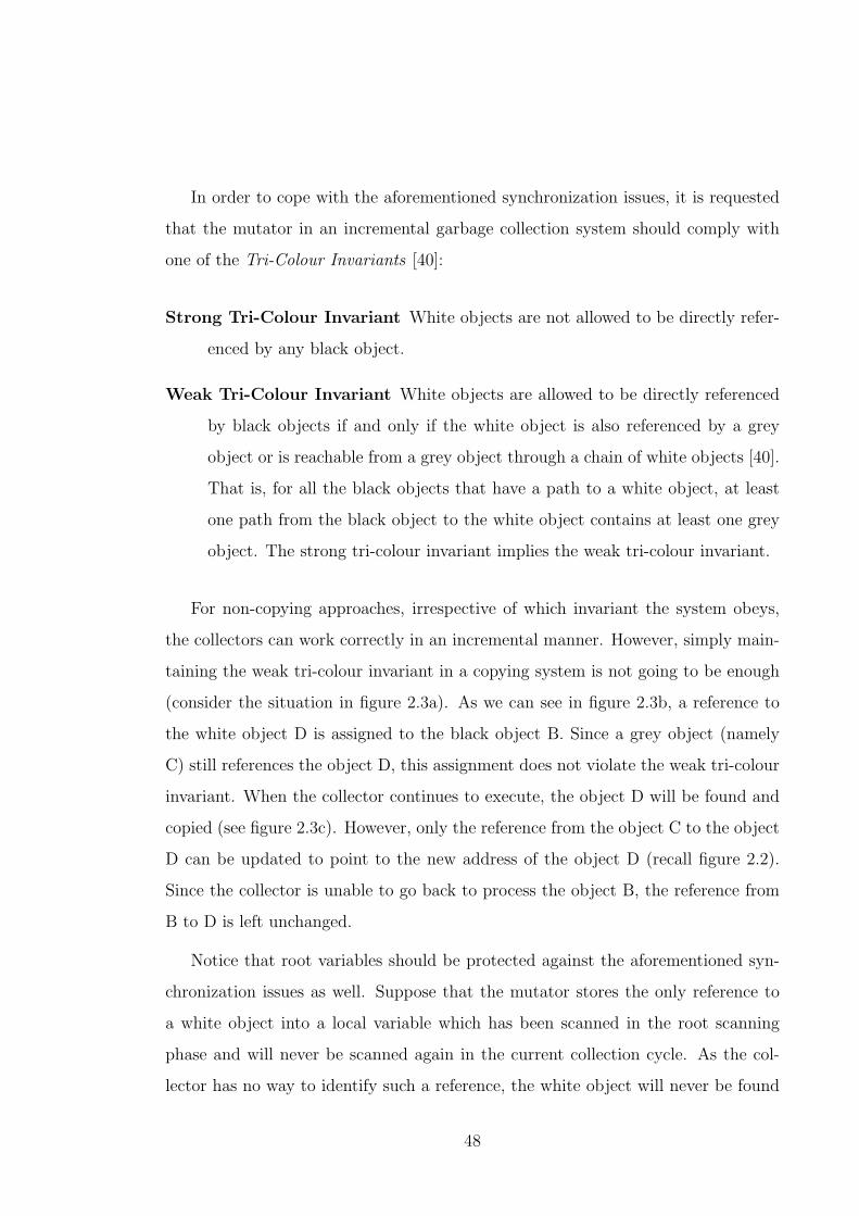
In order to cope with the aforementioned synchronization issues, it is requested

that the mutator in an incremental garbage collection system should comply with

one of the Tri-Colour Invariants [40]:

Strong Tri-Colour Invariant White objects are not allowed to be directly refer-

enced by any black object.

Weak Tri-Colour Invariant White objects are allowed to be directly referenced

by black objects if and only if the white object is also referenced by a grey

object or is reachable from a grey object through a chain of white objects [40].

That is, for all the black objects that have a path to a white object, at least

one path from the black object to the white object contains at least one grey

object. The strong tri-colour invariant implies the weak tri-colour invariant.

For non-copying approaches, irrespective of which invariant the system obeys,

the collectors can work correctly in an incremental manner. However, simply main-

taining the weak tri-colour invariant in a copying system is not going to be enough

(consider the situation in figure 2.3a). As we can see in figure 2.3b, a reference to

the white object D is assigned to the black object B. Since a grey object (namely

C) still references the object D, this assignment does not violate the weak tri-colour

invariant. When the collector continues to execute, the object D will be found and

copied (see figure 2.3c). However, only the reference from the object C to the object

D can be updated to point to the new address of the object D (recall figure 2.2).

Since the collector is unable to go back to process the object B, the reference from

B to D is left unchanged.

Notice that root variables should be protected against the aforementioned syn-

chronization issues as well. Suppose that the mutator stores the only reference to

a white object into a local variable which has been scanned in the root scanning

phase and will never be scanned again in the current collection cycle. As the col-

lector has no way to identify such a reference, the white object will never be found

48

Fromspace Tospace

A B CD

S B

root1 root2

root1 root2

BA

D

C

(a)

A B CD

S B

root1 root2

root1 root2

BA

D

C

(b)

A B

root1 root2

root1 root2

BAC D

BS

C

D

(c)

Figure 2.3: Weak tri-colour invariant: unsuitable for copying algorithms

49

alive. Therefore, it is required to extend the colour scheme and tri-colour invariant

to cover all the roots [79].

At the beginning of a collection cycle, all the roots should be grey, indicating

that root scanning is needed. If some roots have been scanned and the collector

never comes back to rescan these roots, they are said to be black. In a system that

maintains the strong tri-colour invariant, a black root should never point to a white

object. In a system that maintains the weak tri-colour invariant, a black root may

point to a white object if the white object is still reachable from at least a grey

object or a grey root through a chain of white objects.

Not surprisingly, run-time checks are needed on mutator object accesses and, in

some cases, also on root accesses in order to maintain the tri-colour invariants. There

are mainly two kinds of run-time barriers: Read Barriers [13] and Write Barriers

[40, 23, 109], which are pieces of monitoring software or hardware executed in relation

to each load or store operation on references respectively. A good summary of barrier

techniques can be found in [79].

The easiest way to enforce the strong tri-colour invariant is to make sure that no

reference to any white object can be read because such a reference has to be read

before it can be stored in a black object. Read barriers such as [13, 14] monitor

each load operation on references and a white object must be turned to grey before

the reference to it can be read. Although very simple, such a technique can enforce

the strong tri-colour invariant effectively under both copying [13] and non-copying

schemes [14]. However, it has several shortcomings compared with other barrier

techniques:

1. Because triggered whenever the mutator reads a reference, read barriers are

executed much more frequently than any write barrier.

2. At the very beginning of a garbage collection cycle, the mutator’s performance

could be poor [56]. This is because accessing any object at that time (nearly

all the objects at that time are white) may involve a full read barrier execution.

50

3. Such an approach is very conservative because even reading a field of an object

can make it and its children escape from the current collection although they

may actually die very soon. That is, the amount of floating garbage in a read

barrier system is generally higher than many other systems.

As first proposed by Dijkstra et al. in [40], incremental-update write barriers

can be used to enforce the strong tri-colour invariant as well, by checking on each

reference assignment whether a reference to a white object is going to be stored in a

black object. If so, either the black object should be reverted to grey indicating later

rescanning of that object [98], or the white object should be immediately coloured

grey [40]. Normally, it’s easier to understand and prove that a garbage collector

implementing the second algorithm can always terminate since the colour of any

object in the second algorithm can only become darker. Moreover, it is also easier

to implement the second algorithm under a copying scheme. Nevertheless, both

approaches are much more precise than the read barriers so less floating garbage

can be expected in general cases.

What is more, if rescanning of root variables is not performed in an incremental-

update collector, its incremental-update write barriers should also be used to mon-

itor root assignments so that no reference to white object can be stored in a black

root [94, 52]. Notice that, such checks on roots are mandatory even if the root

scanning itself is not incremental.

Another unique write barrier technique, Snapshot-at-beginning, is introduced by

Abrahamson and Patel [1] and later used by Yuasa [109]. Instead of enforcing

the strong tri-colour invariant, this write barrier technique uniquely preserves the

weak tri-colour invariant by only recycling the objects already died before the cur-

rent collection cycle. This is achieved by capturing every reference destruction and

recording the original value (if the object it references is white) in a specific data

structure which will be scanned during the collection. This approach is even more

conservative than read barrier systems in terms of floating garbage (and therefore

51

more conservative than incremental-update systems) since no object can become in-

accessible to the garbage collector while collection is progressing [108]. On the other

hand, a potential benefit of this approach is being safe even without write barriers

attached to root assignments if only the root scanning is performed atomically. This

is because destroying a root reference cannot make the originally referenced object

invisible to the garbage collector since it has been marked. A snapshot-at-beginning

algorithm is guaranteed to terminate because it only registers each white object at

most once and objects’ colour can only become darker in each marking phase. To

date, no other techniques are reported to enforce the weak tri-colour invariant.

Although different barrier techniques could result in different amount of floating

garbage in general cases, the worst-case amount is actually identical. Moreover, if

objects allocated in the current collection cycle are never scanned, a barrier technique

based collector, irrespective of which barriers are used, usually does not scan more

than a given system’s maximum amount of live memory (Steele’s approach is an

exception [98]).

The aforementioned synchronization techniques are not only the fundamental

requirement of incremental garbage collection, but also the cornerstone of concurrent

garbage collection techniques as will be discussed in later sections. Here, emphasis

will be given to some existing incremental tracing algorithms.

2.5.2 Incremental Copying Garbage Collectors

The first incremental copying garbage collector was proposed by Baker [13] and sub-

sequently improved by Brooks [23]. Baker’s approach is essentially an incremental

extension of the Cheney’s algorithm [32] with a read barrier technique.

According to Baker’s algorithm, the garbage collection work is divided into many

small bounded pieces and each of them is associated with an allocation request. More

precisely, whenever the mutator requires to create a new object, a certain amount

of collection work will be performed first and then the new object will be allocated

52

in the current tospace. In order to implement this, a new pointer T is introduced

(see figure 2.4). At the very beginning of a garbage collection cycle, the pointer T

points to the top of the tospace while the pointer S and B both point to the bottom.

The mutator allocates new objects at the position pointed by T and the value of T

is decreased correspondingly.

Since Baker’s algorithm is an incremental one, it must maintain one of the tri-

colour invariants. Here, all the objects in the fromspace are considered white. The

objects located between the bottom of the tospace and the pointer S are considered

black since they have been examined. From the pointer S to B, all the objects

are grey and finally, the pointer T gives a lower bound of newly allocated objects.

Since those newly allocated objects are in tospace and will not be examined by the

collector in the current collection cycle, they are also considered black.

Fromspace

Tospace

White

Free SpaceGrayBlack

S B T

Bottom Top

Newly Allocated Objects(also black)

Figure 2.4: Baker’s incremental copying algorithm

In this algorithm, read barriers provide another chance to do collection work.

When the mutator requires to access an object through its reference while a collec-

tion cycle has already begun, there may be three scenarios:

1. The target object is still in the fromspace.

2. The target object has already been evacuated but the reference still points to

its fromspace copy.

53

3. The target object has already been evacuated and the reference has also been

updated.

In the first scenario, the mutator is reading a reference to a white object. The

read barrier will catch this situation and evacuate the white object to the position

pointed by B immediately (implicitly colour it grey). Of course, since the object has

been moved, the read barrier will update the reference to that object and leave a

forwarding pointer in its old copy. In the second scenario, the mutator is accessing

a reference to the fromspace copy of a black or grey object. First, the read barrier

needs to follow the forwarding pointer to find the correct copy of the object. Second,

it needs to update the old reference to tospace. For the last scenario, the read barrier

needs not do anything. Since the read barrier technique is applied, Baker’s algorithm

maintains the strong tri-colour invariant. Also, the aforementioned disadvantages

of read barriers are inevitable.

When T equals to B or the memory space between T and B is not big enough to

satisfy a new allocation request, the tospace is filled up. If S is currently smaller than

B, which means that the collection work has not been completed, there may still be

some live objects in the fromspace. Since tospace is already filled up, the collector

cannot move them to tospace and accordingly cannot flip the two semispaces. In

order to prevent such an error from happening, it should be guaranteed that enough

garbage collection work is performed in each allocation request so that all the live

objects have already been evacuated to tospace before the pointer T meets the

pointer B.

Baker presents a static analysis to determine how many objects need to be tra-

versed before each allocation so that garbage collection is always finished before

the heap is exhausted [13]. Since the objects in the Lisp language, which Baker’s

algorithm is designed for, have an identical size, it becomes straightforward to argue

that garbage collection work before each allocation be equally long and bounded.

However, the same analysis cannot be applied to other languages directly because

54

objects in other languages can have various sizes and simply counting the number

cannot provide a good enough bound on the real amount of collection work in each

increment.

In addition, Baker presents an incremental root scanning approach as well but

the stack is assumed to be composed of only references [13]. Although not practical

with other programming languages, Baker’s approach demonstrates a way to make

root scanning itself incremental. More details will be discussed in subsection 2.5.4.

Brooks’ algorithm is extended from Baker’s [23]. His most important contribu-

tion is that the read barriers are abandoned. Instead, incremental-update write bar-

riers are used to maintain the strong tri-colour invariant. More specifically, whenever

the mutator requires to write a new value to an existing (object field/root) reference,

the write-barrier will check whether the new value references an object in fromspace.

If so, the object in the fromspace will be evacuated to the tospace, implicitly colour-

ing the object grey. This guarantees that the strong tri-colour invariant can be held

but in a conservative way that even a white object cannot reference any other white

ones.

As discussed previously, in order to guarantee, in Baker’s algorithm, that the

mutator always sees the correct copy of an object, the mutator is not allowed to see

any reference to the fromspace so the read barriers should update such a reference

whenever it is read. Since the read-barriers are discarded in Brooks’ approach, refer-

encing an object in fromspace is now allowed. Therefore, there must be another way

to prevent the wrong copies from being seen. In contrast with Baker’s approach,

every object in Brooks’ system should have a forwarding pointer. When the object

is a fromspace object that has been evacuated to the tospace, its forwarding pointer

points to its tospace counterpart. Otherwise, its forwarding pointer points to it-

self. When the mutator references an object, irrespective of where the object is, its

forwarding pointer always points to its correct copy.

55

2.5.3 Non-Copying Incremental Garbage Collectors

Baker’s Treadmill algorithm is one of the most well known non-copying incremental

garbage collection algorithms, according to which, all the heap objects including free

objects (free memory chunks) are linked together by a cyclic doubly-linked list [14].

In order to distinguish the objects in the free list from the so-called white objects,

the terminology of the tri-colour technique is changed a little bit. The previous

white objects are now considered ecru while the objects in the free list are given

the colour of white. Because the treadmill algorithm is again designed for the Lisp

language, objects are considered with only one size, which greatly simplifies the

garbage collector in hand. Also, similar root scanning techniques as in Baker’s [13]

can be used with the treadmill. Again, the stack is assumed to be composed of only

references.

As illustrated by figure 2.5, all the objects with the same colour are linked to-

gether. Thus, the whole linked-list can be divided into 4 segments. More specifically,

objects with different colours are separated by 4 pointers: free, bottom, top and scan

(see figure 2.5a). When an ecru object is reached by the collector, it is removed

from the ecru set and relinked to the grey set. This also happens when the mutator

reads a reference to an ecru object since Baker takes advantage of the read-barrier

technique to maintain the strong tri-colour invariant. Whenever there is any grey

object, the collector will examine it through the pointer “scan”. After this examina-

tion, the pointer “scan” will be moved one object backward, indicating that the grey

object has already been coloured black. Since this algorithm is an incremental one,

the mutator will probably allocate some objects during a collection cycle. Accord-

ing to this algorithm, the newly allocated objects are coloured black directly. That

is, the free object referenced by the pointer “free” is used to satisfy the mutator’s

allocation requests and then the pointer “free” is moved one object forward. Notice

that each allocation request must be satisfied after a certain amount of collection

work (a GC increment) has been performed.

56

When the pointer “scan” catches up with the pointer “top”, a collection cycle

finishes since no grey object is left. On the other hand, when the pointer “free” meets

the pointer “bottom”, the heap is said to be filled up and a flip must be performed

during the next allocation so that the allocator can find some white objects. If a

collection cycle finishes before the heap is exhausted, the objects finally left in the

heap are of only two colours: either black or ecru (see figure 2.5b). Before the next

allocation request is satisfied, a flip will be performed first. That is, we change

the four pointers to colour the original ecru objects white and colour the original

black objects ecru (see figure 2.5c). Next, the whole algorithm can start over again.

However, if a collection cycle cannot be finished before the pointer “free” catches up

with the pointer “bottom”, some grey objects will be left in the heap, which means

that some live objects may be still in the ecru set so we cannot flip during the

next allocation. Since there are not any white objects anymore, the next allocation

request won’t be satisfied. In order to avoid this situation, we have to guarantee

that enough collection work has been performed before each allocation so that a

garbage collection cycle can be finished before the heap is exhausted.

Requiring that all the objects be of the same size is obviously unacceptable.

Fortunately, it is relatively easy to adapt this algorithm to give it the ability to

process objects with different sizes. The only change is done to the allocator: instead

of simply moving the pointer “free” forward, the allocator needs to adopt some

allocation algorithm discussed in section 1.2 to find a suitable white object to be

allocated. However, the real-time characteristics claimed by Baker will no longer be

achievable with this modification.

Since the read-barrier technique is adopted, this algorithm is also faced with

all the problems introduced by the read barriers (see page 51). Additionally, in

order to maintain such a cyclic doubly-linked list, two pointers have to be added to

each object. However, this algorithm also has some paramount advantages: First,

the garbage collection work is performed incrementally and the WCET of each

increment is predictable. Second, it still reclaims space implicitly. That is, although

57

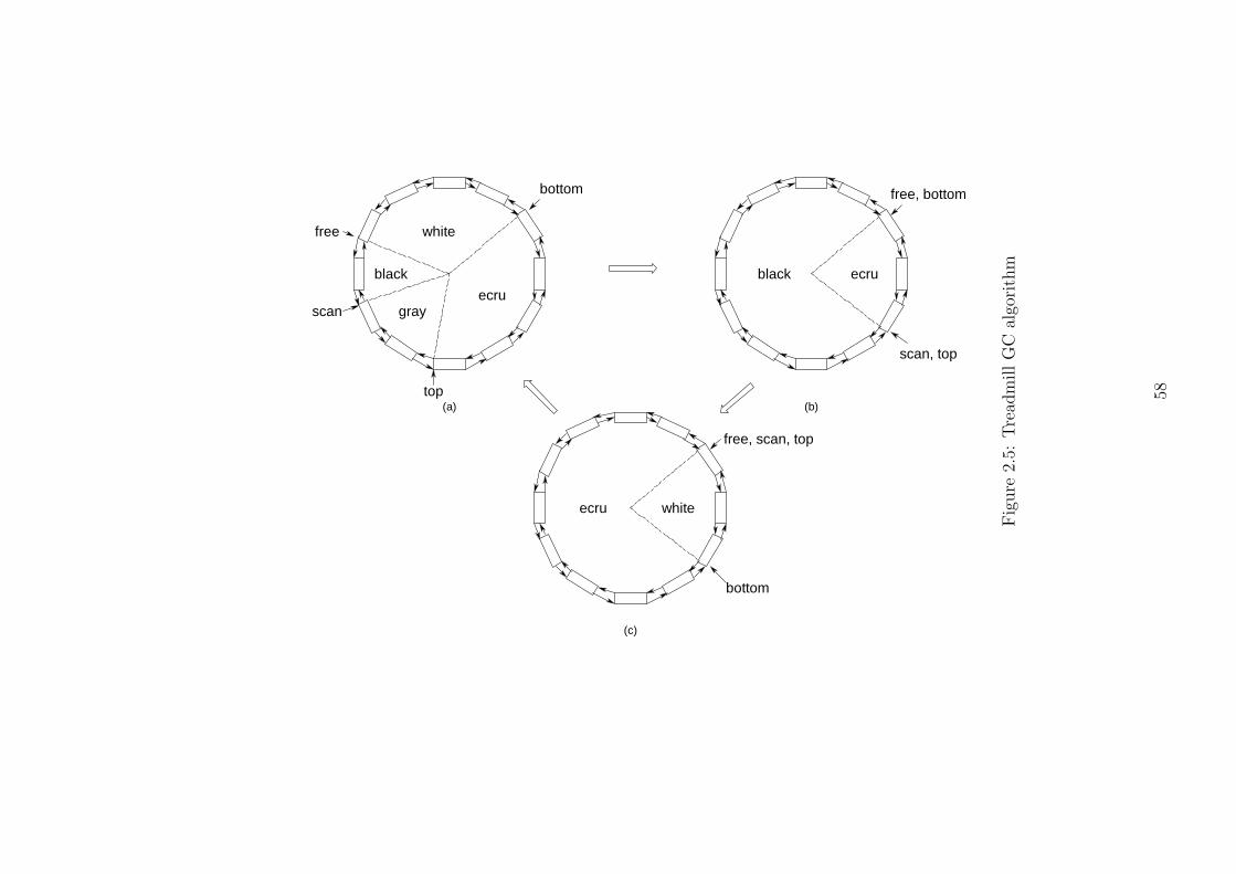
white

grayecru

black black ecru

ecru white

free

scan

top

bottom

free, scan, top

bottom

free, bottom

scan, top

(a) (b)

(c)

Fig

ure

2.5:

Tre

adm

illG

Cal

gori

thm

58

the collector does not really move the objects, the garbage can still be reclaimed in

one action. “Moving” an object now only costs a small constant time regardless of

the object size. Finally, since the objects are not actually moved, there is no need

to update every reference so no forwarding pointer is required.

Yuasa’s work is another well known example of non-copying incremental tracing

garbage collectors, which relies on the snapshot-at-beginning technique to make a

standard mark-sweep algorithm incremental [109]. Two properties are fundamental

to the correctness of this algorithm. First, all objects accessible at the beginning of

a mark phase are eventually marked in that phase. Second, newly allocated objects

during a garbage collection are never collected during the sweep phase. The first

property is ensured by the use of snapshot-at-beginning write barriers on object

reference field assignments. The second one is guaranteed by allocating objects

black during the whole marking phase and a part of the sweeping phase when the

sweeper has not touched the space being allocated.

Again, a stack consisting of only references is assumed to be used by the user

program. In order to scan the stack incrementally and safely while still not impos-

ing any write barrier on root assignments, the stack is copied atomically and the

copied version is scanned incrementally. In addition to the extra space cost, copying

the whole stack atomically may ruin the real-time property as well. Furthermore,

Yuasa proposes to make the system viable where objects with different sizes can be

allocated, by maintaining a free list for each size. However, it is possible, in Yuasa’s

algorithm, that an allocation request is denied when there is enough free memory

which, however, is available in other free lists.

2.5.4 Some Real-time Issues

As previously discussed, real-time systems have unique features which only spe-

cially designed real-time garbage collectors — if any collector would be used —

can support. Making the traversing and reclaiming incremental is merely the first

59

step towards real-time and the remaining steps will be discussed in depth in later

chapters. However, two important prerequisites are going to be explained in this

section.

Incremental Root Scanning

A handful of root scanning, particularly stack scanning techniques have been in-

troduced in subsection 2.3.3, followed by the discussion on other root set related

techniques that are proposed to support incremental traversing and reclamation (in

subsections 2.5.1, 2.5.2 and 2.5.3). Unfortunately, most of them still assume that the

root scanning, itself is performed atomically, and therefore one can easily argue that

root scanning could jeopardise a real-time system’s temporal behaviour (at least in

theory), which otherwise should have been guaranteed by performing other parts

of the garbage collector incrementally. Since performing incremental scanning on

the static data areas and registers are normally straightforward, more emphases will

be put on the stack scanning in this subsection. In order to make the stack scan-

ning incremental, it must be safe to resume the scanner after the user tasks (that

preempted it earlier) give the control back. This is not a trivial problem because

the user stacks may grow or shrink during the execution of the user tasks and their

contents may evolve as well. A scanner must be able to capture such changes — at

least those critical to the safety of the collector.

One thing deserves special mentioning is that some garbage collectors do not

scan “new stack frames”, which are those pushed onto the stack after the stack

scanning commences. In such garbage collectors, the overall stack scanning efforts

will be bounded by the depth of the stack at the beginning of the stack scanning.

In order to achieve this goal, new stack frames must be considered black and barrier

techniques ought to guarantee at least one of the tri-colour invariants.

In a read barrier based system [13, 14], this is automatically guaranteed if only

all the newly allocated objects are considered black or grey.

60

Similar situations can be found in a snapshot-at-beginning system as well [109].

If objects are allocated black or grey, destructing a reference in a new stack frame

will definitely not violate the weak tri-colour invariant even without any write barrier

check because the only white objects that elements of new frames could reference

are those alive at the beginning of the collection cycle. If the other parts of the

stack are scanned correctly, such objects are guaranteed to be seen by the collector

according to the definition of snapshot-at-beginning.

In an incremental-update write barrier based garbage collector, if the write bar-

riers are also used to monitor root variable modifications, references in the “new

stack frames” can never point to a white object without being intercepted by the

write barrier as the “new stack frames” are considered black [94, 52].

The direction in which a stack is scanned has a great influence on the design

of incremental stack scanning algorithms and also on the behaviour of the garbage

collector. If a stack is scanned from the top to bottom, the lowest frame among

all the scanned ones or the highest frame below the scanned ones must be recorded

and compared with the top frame of the stack when a function returns. If the top

frame becomes even lower than the next to be scanned one, the garbage collector

needs to be informed and the next frame to be scanned is updated to the top frame

of the stack. If, however, a stack is scanned from the bottom to top, the highest

frame among all the scanned ones or the lowest frame above the scanned ones must

be recorded instead. Moreover, the lower one between the highest frame that the

garbage collector needs to scan and the top frame of the stack should be continuously

maintained and compared with the next frame to be scanned. If the next frame to be

scanned is higher, the whole stack scanning is completed. Although, at first glance,

scanning from the bottom to top seems to be more complex and expensive, it has a

very interesting feature which could potentially benefit the overall garbage collector

performance. That is, the less active frames are scanned first and therefore the more

active part will be given more chances to change before they can be scanned. This

may provide two advantages, one of which is that more objects may die before they

61

are scanned so less floating garbage could be expected. The other advantage is that

some of the stack frames that otherwise need to be scanned could be popped before

they are scanned so the execution time of stack scanning could be reduced.

Like other parts of the incremental garbage collectors, only a small portion of

the root scanning work is performed each time in conjunction with an allocation.

However, the question is how the work amount should be measured. Previously, it

is assumed that incremental stack scanning can only be interrupted at the boundary

of two frames. More precisely, a stack frame should be scanned atomically. This

could make the control logic more complex since the size of stack frames may vary

dramatically. More importantly, the maximum delay a real-time task may have to

suffer is going to be determined by the maximum size of all the stack frames.

There is one way to solve the aforementioned problem. Instead of scanning each

frame atomically, a certain amount of root references on the stack are processed

as a whole, regardless of the frame(s) in which they reside. Apart from the safety

measures introduced previously, the position where the next to be scanned root

reference is located should also be dynamically updated by the user tasks because

the execution of the user tasks may change the stack layout of the frame currently

under scanning, e.g. by reaching a new gc point with a different stack map. The

next slot to be scanned immediately before the scanner was preempted may become

an invalid reference variable after the control is given back to the scanner. Notice

that the already scanned part of the frames does not need any special action other

than the tri-colour invariant related barriers to ensure safety so the updated (by the

user tasks) position of the reference to be scanned next can only be lower than the

original one (assuming each frame is scanned from high address to low). Despite

the potential benefits, such an algorithm is rarely implemented because of the high

runtime overheads incurred.

As demonstrated previously, Baker’s read barrier based incremental copying col-

lector can perform incremental scanning on a very simple user program stack which

contains only references (stack layout never changes) and each reference is pushed

62

or popped individually [13]. The stack is scanned from the top element when the

scanning begins to the bottom one and every “USER POP” procedure compares

the current top element with the next element to be scanned and updates the next

element to be scanned when it becomes higher than the top element.

A more advanced algorithm called the return barrier is proposed by Yuasa and

integrated with their snapshot-at-beginning collector [110]. Because one of the aims

of this work is to eliminate the write barriers associated with root destructions, it

has to be guaranteed that each stack frame is scanned before its content is modified

by the user tasks. Therefore, the stack has to be scanned from the top to bottom. In

order to achieve this goal, return barriers are introduced to monitor function returns

so that the current frame always resides in the scanned area. More specifically,

every return instruction will be trapped and a barrier code will be executed to check

whether the new top frame has been scanned or not. If it has not been scanned yet,

a certain amount of stack frames will be scanned and only then can control be given

back to the user tasks. Thus, every function return may involve some checking and

stack scanning work, which forces the WCET to be increased.

Another good example of incremental root scanning is Siebert’s approach [93]. As

it is a part of a collector which can provide a certain degree of real-time guarantees,

it will be introduced along with the collector in the next section.

All the approaches that take advantage of the gc point mechanism (except the

one proposed in [99]) have a fatal problem, which makes them unsuitable for de-

manding real-time systems. That is, a high priority task with strict deadlines cannot

preempt the current executing task immediately when it is released. This is because

the current task has to continue executing until it reaches a gc point so that the

correct stack layout can be obtained. Although these delays can be bounded, it is

still undesired in real-time systems which require the switches between tasks to be

performed as fast as possible.

63

Copying Large Objects

The other real-time issue to be discussed here is the delay introduced by copying

large objects in incremental copying algorithms. All the incremental copying algo-

rithms previously discussed in this section build their safety on the basis of atomic

copying of each object. Thus, a real-time task may be delayed by the garbage collec-

tor for a long time when it is copying a large object and the maximum length of such

delays is determined by the maximum size of objects and arrays. If, on the other

hand, the copying process is interruptible, the user tasks may change the contents of

such an object or array. Consequently, the difficulty is that if the field to be accessed

is located in the copied part, its tospace copy must be used and otherwise a recopy

has to be performed. If, however, the field to be accessed locates in the part not

yet copied, the fromspace copy must be used and otherwise an invalid value can be

read or a new value of a field can be overwritten by resuming the garbage collector.

One solution to this problem, as proposed by Henriksson, is to give up the already

copied part of a large object or array when a high priority user task is ready and

recopy the whole object or array when the garbage collector resumes [52]. Normally,

this is an effective approach to avoid the even higher overheads introduced by more

sophisticated and accurate approaches. However, if the length of one execution of

the garbage collector is not long enough to copy the largest object or array, it will

never be copied completely so that the collector cannot progress correctly.

Although all the objects managed by Baker’s algorithm are of the same size, an

extension has been proposed to include arrays and vectors5 [13]. In order not to copy

arrays and vectors atomically, an additional link is required in the header of every

array and vector. Such a link in an array or vector’s fromspace copy points to its

tospace copy and therefore named forward link. On the other hand, the direction of

the link in the corresponding tospace copy is reversed and therefore named backward

link. Another so called scan pointer always points to the next field to be copied.

5In this case, the allocation times are no longer a fixed value.

64

When an access to a partially copied array or vector occurs, the address of the field

to be accessed will be compared with the scan pointer to determine whether it has

been copied or not. If the field has already been copied, the tospace copy will be used

and otherwise the fromspace copy will be accessed. Unfortunately, this approach

requires considerable extra overheads for memory accesses [76, 52].

Nettles and O’Toole propose another solution to this problem in [75]. It is argued

the fromspace copy should always be used before an object is completely copied to

the tospace. However, if any modification is made to the fromspace copy of the

already copied part, such modifications must be logged so that the tospace copy can

be updated to the correct version in due course. Therefore, write barriers must check

the position of the field being modified and log the modification when necessary.

It is also safe to write to both copies but only read the fromspace copy until

the object is fully evacuated. This is because writing to the fromspace copy of an

already copied part makes sure that the subsequent reading operations can get the

updated value. On the other hand, writing to the fromspace copy of a not yet copied

part guarantees that the resumed copying procedure does not overwrite any tospace

slot with an invalid value.

2.5.5 Concurrent Garbage Collection

Incremental garbage collection mainly focuses on two issues: 1) how to make the

garbage collectors and their relevant operations safely interruptible; and 2) how

much work should be performed before each allocation so that both the garbage

collector and the user tasks can progress sufficiently. Intuitively, performing a cer-

tain amount of garbage collection work before each allocation is only one of all the

scheduling choices and it is not necessarily the best one. Concurrent algorithms

share the same techniques with incremental ones to be safely interruptible but they

are executed by a concurrent task which is scheduled along with all the user tasks.

Therefore, when and how long the garbage collector is going to execute will be deter-

65

mined by the scheduler rather than the garbage collector itself (although it can still

influence the scheduler). Next, a comparison between concurrent and incremental

algorithms is given below:

• Generally speaking, incremental garbage collectors can only execute when the

user task is executing. Therefore, the system idle time is simply wasted. On

the other hand, concurrent collectors can take advantage of the system idle

time.

• The collection-work metric is crucial for incremental collectors because a poor

metric could result in unexpected long delays to the user tasks. Concurrent

collectors can be scheduled according to time, which is the ultimate collection-

work metric [87].

• In incremental systems, the user tasks’ execution times have to include the

execution times of the garbage collection increments triggered by their alloca-

tions. This inevitably increments the response times (the time interval between

the release and completion of a task) of the user tasks. On the other hand,

concurrent collectors can make sure that some user tasks’ response times are

never influenced, assuming that enough free memory is always available.

• It is usually easier to guarantee enough progress of the garbage collectors in

the incremental systems since a specific amount of collection work is always

performed before each allocation. Because concurrent collectors are usually

scheduled in a more complex way, it becomes harder to estimate and guarantee

the progress of the collectors.

• Incremental algorithms adopt a very inflexible scheduling approach, which

could be incompatible with the overall scheduling goals and very difficult to

change. The concurrent collectors can be easily scheduled to achieve the overall

scheduling goals and it is much easier to use new scheduling algorithms for

concurrent collectors.

66

There exist advanced concurrent garbage collection algorithms [87, 60, 10, 8, 65].

However, many of them are designed to eliminate costly synchronization operations

and maximize throughput of multi-processor server systems rather than provide

real-time guarantees [8, 65]. Although such algorithms can prevent having to stop

all the mutators for garbage collection at the same time (on different processor),

stopping individual mutator is still required by operations such as root scanning.

Many of the real-time garbage collectors that will be discussed in section 2.7

are concurrently scheduled on single processor platforms. More details of their

concurrency will be presented in that section.

2.6 Contaminated Garbage Collection

Fundamentally, garbage collection is mainly a process of approximating the liveness

of heap objects by computing the (exact or conservative) reachability of those objects

from roots. The most crucial feature that distinguishes one garbage collector from

another is how the object reachability is computed. Reference counting and tracing,

as the two de facto standards of garbage collection, solve the problem by answering

two dramatically different questions:

Reference counting Is there any reference still pointing to a given object?

Tracing Is there a path of references leading to the given object from any root?

Another unique garbage collection algorithm called Contaminated Garbage Col-

lection, is proposed by Cannarozzi et al. to solve the problem by answering another

question [25]:

Which root keeps a group of objects alive and when is that root going to die?

Given a live object in the heap, there is always at least one root referencing it

either directly or indirectly. If there is only one such root, the given object will die at

67

the same time as that root. Otherwise, the object is going to die at the same time as

the last of such roots. In other words, among all the stack frames containing direct

or indirect references to a specific object, the oldest one determines the liveness of

that object and therefore, Cannarozzi et al. define it as the dependent frame of that

object [25].

Intuitively, programs can build references between objects and may consequently

change some objects’ dependent frames because new paths may be built from older

roots to those objects, which happens when an object with an older dependent frame

references another object with a younger one. On the other hand, if a reference

is built in the opposite direction, the ideal situation would be that both objects’

dependent frames should not be changed. However, the dependency relation is

transitive, which means an object with a currently younger dependent frame may be

aged later and the dependent frames of all its descendants may need to be adjusted.

Cannarozzi et al.’s algorithm deals with this transitive nature in a very conserva-

tive way. Every reference built between two objects is considered bidirectional. More

specifically, even if an object with a younger dependent frame references an older

one, both objects’ dependent frames should be the older of the two frames. What’s

more, there is no way to reflect the destruction of the aforementioned reference in

terms of both object’s dependent frames. That is, no object’s dependent frame can

be changed to a younger stack frame throughout its life. The whole algorithm is

described below:

• A newly allocated heap object is considered as an equilive set with a single

element whose dependent frame is the current stack frame [25].

• When a reference to an equilive set is assigned to a static variable, the depen-

dent frame of that equilive set is set to frame 0, which is not popped until the

program finishes.

• When a reference is built between two objects (regardless of the direction)

that belong to different sets, the two sets will be merged into a new one,

68

the dependent frame of which is the older of the two original sets’ dependent

frames.

• When an equilive set is returned from a stack frame to its caller, the dependent

frame of that set should be adjusted so that it is not younger than the caller.

• When a stack frame is popped, all the objects in the equilive sets associated

with this stack frame can be collected.

In order to implement the above algorithm more efficiently, two issues have to

be studied very carefully. First, how to determine the equilive set in which a given

object resides? Secondly, how to merge two equilive sets? The answers to both

questions are paramount to the efficiency and the real-time capability of the whole

algorithm because finding and merging are two most frequently invoked operations

in this algorithm. In the current implementation, Cannarozzi et al. take advantage

of an algorithm introduced by Tarjan, which provides an O(1) complexity merg-

ing operation (excluding the associated finding operation) along with an O(log n)

complexity finding operation with n representing the number of objects in the cor-

responding set [100].

The contaminated garbage collection algorithm has many advantages:

1. Root scanning can be totally eliminated so a lot of overheads are avoided.

2. There is no need to traverse the whole heap to identify live objects before

garbage can be identified.

3. There is no need to understand any application data structure so no type

information is required.

4. The garbage collection work is performed inherently in an incremental way.

However, this algorithm is still not mature. Many disadvantages exist as well:

69

First, it is too conservative. According to Cannarozzi et al.’s algorithm, when

a younger equilive set references an older one, it will be unnecessarily aged. In

addition, this algorithm does not have the ability to turn a set younger when all the

references between it and the older sets are removed. Another source of conservatism

is the way of contaminating two objects. In the current algorithm, when two objects

contaminate each other, the two sets to which the objects belong are merged as a new

set. This is conservative because some objects in the two sets may be unnecessarily

aged.

Second, there is a situation that the current algorithm cannot deal with: when a

method with a pretty long lifetime (for example, a method that includes very long

or even unbounded loops) is invoked, all the older stack frames and itself cannot be

popped for a long time, which means that all the equilive sets associated with these

stack frames cannot be reclaimed for a long time. It is even worse if the long-lived

methods can allocate new objects constantly, the heap will be exhausted sooner or

later.

In addition, Cannarozzi et al.’s algorithm does not resolve the fragmentation

problem. Although they provide a special way to determine what is garbage, they

do not show any new idea about how to reclaim garbage. All the garbage objects

are still reclaimed one by one just like what happens in the mark-sweep garbage

collection. Therefore, fragmentation problem is inevitable.

2.7 State-of-the-art Real-time Garbage Collection

Algorithms discussed in this chapter so far are not able to provide real-time guar-

antees to state-of-the-art real-time applications. Neither are they integrated with

real-time scheduling schemes. Although some incremental algorithms can exhibit

very limited real-time behaviours by distributing the garbage collection work and

ensuring that every memory related operation has an upper bound on its execution

70

time, these algorithms lack the supports to some important language features that

can be easily found in modern programming languages (e.g. variable size objects).

Furthermore, the targeted task model is still not a typical real-time one and no real-

time scheduling requirement is considered. In this section, some garbage collectors

with more sophisticated real-time supports and with more modern language features

in consideration will be introduced.

2.7.1 Henriksson’s Algorithm

First of all, Henriksson’s semi-concurrent algorithm6 provides explicit supports to

periodic real-time tasks under fixed priority scheduling. Hard real-time tasks’ prior-

ities are strictly higher than those of the other tasks. In order to reduce the WCETs

of hard real-time tasks and consequently make the scheduling easier, garbage collec-

tion work caused by the memory related operations performed by the hard real-time

tasks is delayed and performed by a segregated task (the GC task) running at a pri-

ority between the hard real-time tasks and the others. The tasks with lower priorities

than the GC task still have to perform collection work in each allocation.

Henriksson’s collection algorithm is based on Brooks’ write barrier based incre-

mental copying scheme as described in section 2.5.2. However, instead of evacuating

a fromspace object immediately in a write barrier, such an operation is delayed to be

performed later by the collector. By performing such lazy evacuation, the WCETs

of hard real-time tasks can be reduced. In such a new write barrier, if the object in

question has not yet been copied to tospace, memory space will be reserved in the

tospace for it and the tospace copy’s forwarding pointer will be set to point back

to the fromspace copy so that accessing to the tospace copy is actually redirected

to the fromspace copy. On the other hand, the forwarding pointer in the fromspace

is left unchanged but an additional flag word is set to point to the tospace copy to

6 So far as we know, Henriksson’s algorithm is the only example of the semi-concurrent algo-

rithm. It is a combination of incremental and concurrent scheduling.

71

inform later write barrier checks that this object has already got a reserved area in

tospace. Note that this technique is applied to all the tasks in Henriksson’s system

in order to get smaller code size.

Object initialization (which means fill the whole memory block that will be

allocated to the object with zero) is also moved from the hard real-time allocators

to the GC task but the garbage collector must always ensure that enough free

memory is initialized to meet the requirements of the hard real-time tasks. This is

partially achieved by asking the GC task to initialize a memory area of size MHP

— big enough to satisfy the worst-case memory requirements of the hard real-time

tasks during one release of the GC task — every time it is activated. In addition,

the low priority task’s allocators must initialize the same amount of memory as the

requested size before an allocation can be performed. Also, the garbage collector

is required to initialize an area of size MHP in fromspace before a flip can happen

in order to ensure that the hard real-time tasks can allocate in the new tospace

immediately after a flip. This adds to the total work of the garbage collector.

In order to prevent the deadlock of copying scheme from happening, all the live

objects must be evacuated before a flip is requested. In the work discussed in section

2.5.2, this is enforced by performing sufficient garbage collection work before each

allocation. Henriksson follows a similar way so that each allocation is associated

with a certain amount of collection work but the hard real-time allocations’ collec-

tion work is performed later by the GC task. A more sophisticated estimation of the

minimum GC ratio, which defines the minimum sufficient collection work in connec-

tion with an unit of allocation, is given along with more accurate work metrics other

than simply counting the evacuated memory as a measure of performed collection

work. More importantly, real-time schedulability analysis can be performed for all

the hard real-time tasks including the GC task.

One of the outstanding issues of this work is that separate stacks consisting of

only the addresses of references have to be manually maintained by programmers for

the references on the program stacks due to the inability to perform exact stack scan-

72

ning. In addition to the unnecessary burdens on programmers, expensive runtime

overheads have to be paid. What is more, although Henriksson claims incremental

stack scanning, it is not clear in his thesis how this is achieved.

2.7.2 Siebert’s Algorithm

Siebert published several papers and a thesis to present his unique Dijkstra style

write barrier based incremental mark-sweep garbage collector which is claimed to

be real-time [90, 91, 89, 92, 93, 95, 94]. One of his two major contributions is the

introduction of a new way to eliminate fragmentation. Instead of moving objects to

compact the heap, which inevitably incurs huge overheads as discussed in previous

sections of this chapter, Siebert’s system organizes the heap as an array of fixed size

blocks. Program objects and arrays are all built out of such blocks but objects are

organized as linked lists of blocks while arrays are organized as trees [92]. One could

argue that such a scheme simply transforms external fragmentation into internal

fragmentation but internal fragmentation is preferred to either external fragmenta-

tion or moving objects in a real-time application because it is much easier to predict

and has less overheads. Apart from the space overheads incurred by internal frag-

mentation and additional links that are used to maintain objects and arrays, extra

memory accesses could be required when accessing a field in the heap to follow the

links to find the proper block. Siebert studies such overheads and claims that they

should be acceptable in languages like Java [92, 94] (because most objects tend to be

small in such languages). It is also believed that reasonable WCETs of field accesses

can be obtained.

In order to cooperate with such a new heap organization, the garbage collec-

tor marks and sweeps individual bocks rather than a whole object or array. Links

between blocks within an object or array are treated in the same way as user de-

fined references. Since blocks are coloured individually, an object or array could be

composed of blocks with different colours but tri-colour invariant must be held for

73

those internal links as well. Note that Siebert’s system allocates objects grey so they

need to be scanned even in the garbage collection cycle in which they are created.

Furthermore, in order to find exact references in the heap, a bit vector (each word

in the heap corresponds to a bit) must be maintained for the whole heap, which

inevitably introduces both extra time and space overheads.

As an incremental collector, this algorithm requires that a certain amount of

garbage collection operations proportional to the requested size be performed at each

allocation. Because exact root scanning is required, synchronization points are set

in Siebert’s system and therefore, context switches and garbage collection are only

allowed at such points. In order to reduce the latency caused by garbage collection

to a minimum constant value, a synchronization point is added after marking or

sweeping each single block so that a single increment of garbage collection work is

also preemptable.

The other major contribution of Siebert’s research is a new stack scanning ap-

proach, which argues that any root reference (in any task’s stack) with a lifespan

that stretches over at least one synchronization point should present itself in a heap

data structure called root array at every such synchronization point(s) only, by ex-

ecuting some compiler generated codes. Consequently, whenever root scanning is

due, all the active roots are already in the root arrays. A root array is maintained

for each task and all the root arrays are organized by a single list which is referenced

by a single global root pointer. So, in Siebert’s system, there is actually only one

root (all the roots in the registers and static data areas are also copied into the

heap) and the actual root scanning is integrated into the marking phase. All the

root arrays are in the heap and thus protected by the strong tri-colour invariant so

it is guaranteed that no root reference can be lost. However, it is not clear how the

root arrays are implemented so the answers to two questions cannot be found in any

of Siebert’s publications so far:

1. Are the new roots added to the root arrays after the root scanning begins going

74

to be scanned? As discussed previously, these roots do not actually need any

scanning (since incremental-update write barriers are used to monitor root

modifications).

2. Since the mutators may change the root arrays’ layouts, how is the garbage

collector informed of such information?

Apart from the overheads of saving and deleting live roots around synchroniza-

tion points, extra space overheads introduced by root arrays are also not welcomed.

Siebert proposes both static and dynamic approaches to make sure that enough

collection work is done in each increment so that the application never runs out of

memory. In the static approach, by selecting a constant ratio P = 2/(1−k) where k

is the maximum fraction of live memory (compared with the heap size) and scanning

P units of allocated memory whenever one unit memory is to be allocated, garbage

collection is always guaranteed to complete before free memory is exhausted. On the

other hand, a more flexible approach to provide the same guarantee is to substitute

the constant ratio P with a progress function P (f) = 1/f where f is the current

fraction of free memory compared with the heap size again. An upper bound of

this progress function can also be deducted so that the length of each collection

increment is still bounded.

As demonstrated by Siebert in [89, 94], the average performance of the dynamic

approach is much better than its static counterparts since very little collection work

is needed when f is large. However, the maximum value of P (f) is normally much

higher than the constant ratio P given that the values of k are identical so the

estimated WCETs of user tasks under the dynamic approach are much higher. In a

hard real-time system, the static approach is more likely to be preferred. What is

more, the experiment results presented in [94] justifies the time-space tradeoff in such

a garbage-collected system. In both the static and dynamic approaches, the values

of P and P (f) can be reduced by increasing the heap size and therefore decreasing

k. Note that the garbage collector in question integrates the actual root scanning

75

with the marking phase so memory occupied by the roots should be included in k

as well.

2.7.3 Ritzau’s Reference Counting Algorithm

As discussed in section 2.2, the cascading deallocation problem can be partially

resolved by the lazy freeing technique. However, deterministic behaviour cannot

be obtained because buffered objects are of different sizes which are not necessarily

suitable for allocation requests. In other words, the time needed to satisfy an alloca-

tion request cannot be reasonably bounded or new free memory has to be requested

which makes the spatial behaviour less predictable.

Ritzau uses a similar approach to the one proposed by Siebert [92] to solve

the aforementioned problems [83]. Again, objects and arrays are built out of fixed

size blocks and maintained as linked lists or trees so external fragmentation can be

eliminated at the expense of the more predictable internal fragmentation. As blocks

can be reclaimed independently, the size of the first object in the to-be-free-list — the

data structure used to buffer those objects already found dead — no longer bothers

the allocator. More precisely, the allocator only reclaims the exact number of blocks

as requested irrespective of whether the object under processing is fully reclaimed

or whether the blocks are in the same object. By doing so, the execution time of

the allocator becomes proportional to the requested size and therefore bounded.

In contrast with all the algorithms discussed so far, the predicted temporal be-

haviours of allocations in Ritzau’s algorithm are not influenced by the heap size

even when it is as small as the maximum amount of live memory (recalling that the

P and P (f) of Siebert’s approach could be unlimited if k is assumed 100%). That

is, the user tasks can reuse dead object’s memory whenever they need. However,

Ritzau did not resolve the cyclic garbage problem in his work so the aforementioned

characteristic can only be achieved with the absence of cyclic data structures.

76

2.7.4 Metronome Garbage Collector

All the aforementioned systems, except the hard real-time part of Henriksson’s sys-

tem, perform garbage collection work in each allocation so they are characterized as

work-based. As argued by Bacon et al., such algorithms could suffer from close to

zero mutator utilizations7 during bursty allocations although individual pauses by

garbage collection are kept under control [11]. Motivated by such a concern, Bacon

et al. proposed a time-based scheduling scheme for garbage collection under which

garbage collection quanta with fixed lengths are scheduled at fixed rate in terms of

time. During each collector quantum, no user task can execute and vice versa. By

doing so, a minimum mutator utilization can be guaranteed throughout the whole

life time of the application because the collector cannot consume more than a collec-

tor quantum each time it is scheduled and cannot be scheduled more frequently than

the given rate. From the real-time terminology’s point of view, this is essentially

a simple polling server system [88] in which the collection work is performed by a

periodic server with the highest priority.

The collector itself is a mostly non-copying snapshot-at-beginning one which

performs defragmentation when needed and allocates new objects black. The heap

is divided into equally sized pages (not the system page) each of which is further

divided into blocks of a particular size. The size of blocks varies from one page to

another and an object can only be allocated in a block of its size class. The allocator

uses segregated free lists for different size classes to make external fragmentation

generally low. However, the problem has not been completely solved so objects in

less occupied pages must be copied to more occupied pages of their size class. As

claimed in [11], the amount of such copying work is generally low in a handful of

benchmarks compared with pure copying schemes.

Due to the defragmentation work, the Brooks-style forwarding pointers [23] are

7 The mutator utilization is defined as the mutator execution time during a given time interval

divided by the length of that interval [11].

77

introduced to ensure that the correct copy of any object can always be seen. It is

shown in their experiments that the mean cost of such operations after optimizations

can be as low as 4% while the observed worst-case cost is 9.6% [9]. On the other

hand, it is by far still not clear how expensive the snapshot-at-beginning write

barriers are.

Because root scanning is still an atomic operation in Metronome collector, snapshot-

at-beginning write barriers are not needed to monitor root modifications (recall that

new stack frames need not be monitored in a snapshot-at-beginning system). Cur-

rently, the real-time guarantees are given under the hypothesis that scanning the

whole program stack always takes shorter time than a collector quantum. In the

future, we cannot see any reason why the Yuasa-style return barriers cannot be

implemented in Metronome to make the root scanning phase interruptible [110].

Bacon et al. also present a static analysis to explore the space bound of any

given application under Metronome. The factors influencing the bound most are

the maximum amount of live memory, the garbage collector processing rate (ac-

tually marking rate), the lengths of each collector quantum and mutator quantum

and finally the average allocation rate of the program. The size of the redundant

memory buffer required during one collection cycle is the amount of all the allo-

cation requests raised during that period. However, due to floating garbage and

object copying, three such redundant memory buffers are needed in the worst case

although this worst case is very unlikely to happen. Note that two assumptions

must be satisfied before the analysis can be claimed correct [11]. First, it is as-

sumed that the collection cost is totally dominated by the marking phase. Second,

it assumes that the actual amount of allocation requests during a collection cycle is

always lower than the average allocation rate multiplied by the mutator execution

time during that period. For the first assumption, sweeping and defragmentation

phases may execute for non-trivial amounts of time relative to the marking phase so

the estimated length of the current collection cycle may be shorter than the fact and

therefore, the excessive space may be underestimated. For the second assumption,

78

using the average allocation rate is not “hard” enough because the actual memory

usage may be worse than the average case in some collection cycles. Moreover, all

the results given in [11] are empirical observations rather than theoretical bounds.

For example, although the presented ratios between heap sizes and the maximum

amounts of live memory are all below 2.5, the theoretical bounds are actually much

higher than that according to the analysis under discussion.

In another paper [9], Bacon attempts to relax the first assumption by refining

the collection cost model. This requires additional parameters, some of which are

difficult to obtain. Moreover, the new model introduces another assumption that

the heap never exceeds 2.5 times the size of the maximum amount of live memory

in order to estimate the sweeping phase cost in a straightforward way. Otherwise,

a recurrence relationship between the heap size and the sweeping phase cost has to

be resolved. This is because the sweeping phase cost depends on the heap size while

the heap size can only be estimated if the collection cost is known already. The

expansion factor, as defined in [9], is assigned as 2.5 because no heap is 2.5 times

larger than the maximum amount of live memory in all the experiments. Again,

this is not a theoretical bound.

In a further discussion of Bacon’s work, more details of the collector are revealed

[10]. First, the potential pauses caused by copying large chunks of memory atom-

ically have not been eliminated in the current algorithm. Therefore, an abortable

copying approach is proposed to solve the problem in the future work. It is also

noticed that if the recopyings are performed too frequently, the collector would

hardly progress. In addition, such costs should be modeled into the overall collector

cost. Moreover, it is revealed that synchronization points and restricted context

switches are required in the current system. Thus, a more sophisticated analysis of

synchronization points to reduce the pause time is put into the “to-do” list as well.

79

2.7.5 Kim et al.’s Algorithm

Kim et al. design a copying garbage collector for hard real-time systems which are

only composed of periodic user tasks under fixed priority scheduling [60, 61]. It is

assumed that there is no precedence relation between the tasks and preemptions can

be immediately executed when needed.

The collection algorithm is based on Brooks’ work which is an incremental-

update write barrier based copying algorithm [23]. In order to reduce the write

barrier overheads and execute user code faster, a mechanism similar to Henriksson’s

lazy evacuation is proposed. More specifically, write barriers only reserve memory

in tospace and setup the forwarding pointers, leaving the actual evacuation to the

garbage collector by recording the reference modifications in the so called update

entry. At the end of each collection cycle, the update entry is checked and all the

pending evacuations are performed.

Although nothing has been said about how exact root information is obtained

[58, 60], Kim et al.’s incremental root scanning algorithm is doubtless an interesting

one for real-time systems. It is argued that the root scanning and heap traversing

should be performed one task after another in a longest-period-first order instead of

scanning all the tasks’ stacks and then traversing the whole heap [58, 60]. By doing

so, the more frequently changing stacks are processed later than the less frequently

changing ones. Also, the scanning of each task stack is followed immediately by

traversing objects referenced by that task. This change may give the tasks with

short periods more chances to mutate before the objects referenced by those tasks

are traversed. Thus, less floating garbage can be expected in general. In addition,

the actual evacuation of objects directly referenced by roots is delayed until the

current root scanning completes and then performed incrementally.

Because each semispace of such a system is bounded by the maximum amount of

live memory plus the maximum amount of all the allocation requests raised during

any collection cycle, scheduling the garbage collector in a way that it finishes earlier

80

may potentially reduce the amount of excessive memory and therefore the overall

memory requirements. In Kim et al.’s system, the garbage collector is considered as

an aperiodic task. It is a specific memory usage event rather than a timer expiration

that triggers a garbage collection cycle. In order to schedule the whole system in

favour of garbage collection while guaranteeing the user tasks’ deadlines, a sporadic

server is introduced at the highest priority8. With the sporadic server technique, the

worst-case response time of a garbage collector can be estimated given the WCET

of that collector.

As for all the other work presented in this section, Kim et al. do offer a static

analysis to estimate excessive memory and the overall memory requirements [60].

In order to do so, the WCET of the collector must be known beforehand and then

a standard method can be used to estimate the worst-case response time of the

collector running in the sporadic server [60]. Given the collector’s worst-case re-

sponse time, the number of instances of each task released during that time can be

calculated and therefore, the worst-case memory consumption during the collector’s

worst-case response time can be determined [60]. The sum of this value and the

maximum amount of live memory is used as the size of each semispace. Compared

with background policy, this new scheduling approach allows a 16% – 42% improve-

ment on the worst-case memory bound (theoretical) of the whole system in some

given applications [59]. Moreover, the schedulability of the whole system including

both the mutators and the collector can be guaranteed as well.

Another contribution of Kim et al.’s work is a live memory analysis which is

designed specifically for real-time systems consisting of periodic tasks. Rather than

another data flow analysis, Kim et al.’s efforts mainly focus on getting a more accu-

rate overall live memory bound given the amount of live memory of each task [60].

By noticing that when inactive (waiting for the next period), a task’s contribution

to the overall live memory is normally lower than when it is active, the overall live

8 It also has the shortest period because rate monotonic scheme is used to determine the

priorities of all the tasks.

81

memory at a certain time can be more accurately described as the sum of the active

tasks’ full live memory and the inactive tasks’ reduced live memory. How much the

difference is between a task’s full live memory and its reduced version is considered

as an input of programmers or some automatic tools so it is not discussed in any of

Kim et al.’s work. On the other hand, it is now crucial to find out all the preemp-

tion relations so that all the combinations of active tasks and inactive tasks can be

determined, which is then used to estimate the worst-case live memory. As claimed

by Kim et al., this new analysis allows a 18% – 35% reduction in the maximum

amount of live memory (excluding the global objects used by all the tasks) in some

given applications [60].

Although the use of another aperiodic server to execute soft user tasks is ruled

out by Kim et al. [60], a dual aperiodic server scheduling scheme under which both

servers execute the garbage collector only is designed [61]. The main purpose of

doing so is to overcome the often extreme low server capacity at the highest priority

as in [60]. By introducing another aperiodic server at a lower priority but with a

higher capacity, only the initial steps of a collection such as flipping and memory

initialization are to be performed by the aperiodic server at the highest priority

while the other steps are to be executed by the low priority server. A new response

time analysis and consequently a new worst-case memory requirement analysis are

introduced as well.

2.7.6 Robertz et al.’s Algorithm

Robertz et al. propose another approach to schedule garbage collection in a real-time

system consisting of periodic tasks [87]. An incremental mark-compact algorithm is

assumed to be scheduled but very little information has been released on how this

collector works. It is also not clear how the root scanning is performed in such a

collector. First, it is argued that the oversimplified collection work metrics used by

most work-based incremental algorithms are troublesome when real-time guaran-

82

tee is the primary goal. Although better metrics are available, they become rather

complex. In Robertz et al.’s algorithm, the garbage collector is considered as a seg-

regated task and scheduled in the same way as user tasks but with a deadline equal

to its period. Any specific scheduling algorithm that suites this model, such as ear-

liest deadline first or fixed priority scheduling, is allowed. Given the characteristics

of user tasks, heap size and the maximum amount of live memory, the period (and

the deadline) of the garbage collector can be estimated so that the system never

runs out of memory if only the garbage collector always meets its deadline.

2.8 Summary

In this chapter, we first presented some classical non-real-time garbage collection

algorithms and relevant techniques. Among them, the reference counting, incre-

mental tracing, concurrent scheduling, exact and incremental root scanning along

with interruptible object copying algorithms are the most concerned ones to us.

A few state-of-the-art real-time garbage collectors developed on the basis of these

algorithms were introduced as well. A brief summary of these real-time garbage

collection algorithms can be found in table 2.1.

83

Algorithms Sibert’s Henriksson’s Robertz etal.’s

Ritzau’s Metronome Kim et al.’s

Basic Col-lectionAlgorithm

mark-sweep copying mark-compact

referencecounting

mark-sweep(withcopying)

copying

Barrier incremental-update writebarrier

incremental-update writebarrier

not clear write bar-rier

snapshot-at-beginningwrite bar-rier

incremental-updatewrite bar-rier

Scheduling incremental semi-concurrent

concurrent incremental concurrent concurrent

ObjectCopying

— interruptible not clear — atomic not clear

Exact RootScanning

yes yes not clear — yes not clear

IncrementalRoot Scan-ning

yes yes not clear — no yes

Table 2.1: A brief summary of the state-of-the-art real-time garbage collection al-gorithms

84

Chapter 3

New Design Criteria for

Real-Time Garbage Collection

Garbage collector design criteria suitable for real-time environments are crucial for

the next generation flexible real-time systems. In spite of those existing ones that

are claimed to be “real-time”, more sophisticated real-time garbage collector de-

sign criteria are proposed in this chapter. First of all, some major problems with

the state-of-the-art real-time garbage collection techniques are presented along with

detailed explanations on those that could have been (at least, partially) avoided

with better design criteria. Then, new design criteria are proposed in the hope

that new garbage collectors designed under these criteria do not experience the

aforementioned problems, or at least suffer less. Finally, some existing literature

already discussed in the previous chapter is revisited to explore their effectiveness

or potential to become effective according to our new criteria.

3.1 Problem Statements

The state-of-the-art real-time garbage collectors are always criticized for their inef-

ficiency in either the space or time dimension. Although good results in any one

85

dimension can be obtained, they can be hardly observed simultaneously. Signifi-

cantly improving the performance in one dimension would bring serious penalties to

the other one. Achieving the right balance with satisfactory performance in both di-

mensions is far from trivial, which forces many new generation real-time platforms,

such as RTSJ, not to rely on real-time garbage collection techniques but seek for

other alternatives in which extra programmer efforts and new programming patterns

are normally required.

Siebert’s garbage collector shows very good examples of this problem [94]. In its

dynamic configuration, the number of blocks needed to be processed before every

allocation of one block is P (f) = 1/f where f denotes the current fraction of free

memory compared with the heap size (for more details, see subsection 2.7.2). On the

one hand, if P (f) can be always kept low, the slowing down of the application due

to garbage collection can be eased. If, on the other hand, f is kept to a minimum,

the overall memory requirements will be no more than just a little bit higher than

the maximum amount of live memory. According to the analysis presented in [94],

P (f) and f can be as low as one and zero respectively, which seems to be an

astonishing result. Unfortunately, this can never be achieved simultaneously in a

single application. More specifically, when P (f) = 1, f must be one as well, which

means that the whole heap is free; when f = 0, P (f) must be unlimited, which

means that the garbage collector degrades to a stop-the-world one. Between the

two extreme cases, Siebert reports a series of analytical results, which demonstrate

the relationship between the maximum amount of live memory, heap size and the

worst-case value of P (f) under such a dynamic configuration [94].

When the maximum amount of live memory is set to be only 0.3 of the heap

size, the worst-case number of blocks that must be processed before an allocation

will be 6.173 times the number of blocks requested. When the ratio between the

live memory and the heap, k, is set to a reasonable value of 0.8, the collection work

is going to occasionally reach 33.1 times the number of blocks requested. When the

static configuration is applied, the collection work for each block allocated becomes

86

stable. If k is again set to 0.8, the amount of collection work will be fixed at 10

times the number of blocks requested, which is still quite high. By decreasing k

to 0.3, which means the heap becomes 3.33 times the size of what is really needed,

the amount of collection work can be reduced to 2.86 times the number of blocks

requested. In conclusion, high space overheads are inevitable in Siebert’s collector

when the temporal overheads are kept low and vice versa.

Many other collectors exhibit similar behaviours. For example, the overall heap

size of a Metronome system is bounded in the worst case by m + 3e where m is the

maximum amount of live memory and e is the memory required to run the applica-

tion without any delay (due to the lack of free memory) during a single collection

cycle [11]. By executing the collector 12.2ms out of every 22.2ms (45% mutator

utilization), several SPECjvm98 benchmarks are performed and the observed ex-

pansions of the heap size over the maximum amount of live memory are never higher

than 2.5 times throughout these tests. However, such an observed expansion factor

only resembles the expected space usage m + e rather than the theoretical bound

m + 3e. Therefore, according to a brief calculation, the worst-case bound of such

an expansion factor could reach as high as around 5 in some of the aforementioned

benchmarks.

In their later publication [10], it is claimed that parameters including the period

of the polling server that executes the garbage collector, and either the utilization of

the server ut, or the overall heap size h are tunable. Although neither empirical nor

analytical results are presented, it is argued that the last two parameters mutually

influence each other and intuitively, relaxing the limitations on server capacity would

reduce the overall memory requirements and vice versa. If the server utilization is

reduced to below 55% (mutator utilization will be higher than 45%), the expansion

factors will be further increased to perhaps even higher than 5.

Another good example is Kim et al.’s aperiodic server based copying collector

[60]. As the server (which executes the collector) utilization is tuned from 10%

to 23%, the expansion factor of a specific task set’s heap size over its maximum

87

amount of local live memory1 is decreased from 7.03 to 6.59. Note that the expansion

factors here are not directly comparable with those of the Siebert’s system and the

Metronome because only a portion of the maximum amount of live memory is used

as the reference here since the overall live memory information is not available for

this task set.

Another outstanding issue to be resolved is how to better schedule a garbage-

collected real-time system. It was not possible to perform schedulability analysis

of a garbage-collected real-time system until Henriksson introduced his scheduling

scheme and analysis in [52]. However, the GC task is fixed at the highest priority

below all the hard real-time tasks, which makes the system very inflexible. When the

hard real-time tasks’ load is high, there will be very little chance for the GC task to

progress sufficiently and therefore, more excess memory may be needed. Moreover,

the soft- or non-real-time tasks can only be executed at priorities even lower than

the GC task, which may result in poor response time of such tasks and eventually

poor system utility and efficiency. Robertz and Henriksson later proposed another

scheduling scheme for garbage-collected real-time systems, according to which the

garbage collector is transformed into a periodic hard real-time task with a period,

deadline and WCET and thus, virtually any hard real-time scheduling scheme and

analysis currently available can be used in such a system without any modification

[87]. However, it is also assumed that all the user tasks should be periodic real-time

tasks.

By contrast, Metronome and Kim et al.’s system see collectors as aperiodic

soft-real-time tasks which are driven by specific memory related events. On the

one hand, all the hard real-time user tasks can be easily analyzed with the same

method as the corresponding traditional server-based real-time systems use. On the

other hand, guaranteeing enough progress of the collector under such schemes is

not trivial. Specially designed analysis must be conducted. Furthermore, there is

again no consideration of combining different types of user tasks. More advanced

1 Here, local live memory means the live memory that is not shared between tasks.

88

scheduling schemes and analyses along with better integrations of the collectors and

the current scheduling frameworks are still needed.

As discussed previously in sections 2.3 and 2.5, both finding roots exactly and

scanning them incrementally are very complex and expensive, which normally in-

volves write barriers on roots, delayed context switches, extra management data

or specialized function returns. So far as we know, there is still no perfect solu-

tion to these problems although great efforts have been made in many directions

[94, 60, 110]. In Siebert’s system, root scanning is merged into the marking phase,

although extra copies and deletions of roots must be performed at many synchro-

nization points. Moreover, write barriers on roots are necessary for safety reasons

and presumably, method returns need to be monitored as well. By contrast, Yuasa

eliminates write barriers on roots by introducing heavier method returns. However,

this approach is only viable in snapshot-at-beginning systems and no further infor-

mation is given on how to exactly identify roots (synchronization points may be

still needed). Note that many factors contribute to the context switch delays which

should be avoided in real-time systems, particularly the hard real-time ones. Above

all, context switches may be limited to the synchronization points because exact

root information is only available at those points. The worst-case delay (due to syn-

chronization points) of any task in such a system is the maximum length between

any two consecutive synchronization points throughout the whole system. When

calculating the response time of any task, this factor must be counted in. Secondly,

parts of the root set (such as a task’s stack or a stack frame) or even the whole

of it must be scanned atomically. Finally, some primitive operations such as the

specialized method returns must be performed atomically as well.

Apart from all these problems, how to interrupt the copying of a large object

efficiently and resume it safely is also crucial for the success of a copying collector in a

real-time environment. Although several approaches have been discussed in section

2.5.4, they all rely on heavy barriers on memory accesses or performing potentially

unbounded recopying to achieve the aforementioned goal. So far as we know, there

89

is no perfect solution to this problem.

Our collector (see later chapters) does not suffer from any of the aforementioned

problems.

3.2 Decomposition of the Overall Memory Re-

quirements and Garbage Collection Granular-

ity

Ideally, the overall memory requirements of a garbage-collected system should be

identical to its maximum amount of live memory and any memory requirement

beyond that is deemed as overheads which should be minimized. In those primi-

tive stop-the-world mark-sweep (assuming fragmentations never occur) and mark-

compact systems, the ideal result can be achieved since all the dead objects can

be reclaimed before a new one comes into existence even when there is already no

free memory. However, real-time systems cannot afford to be suspended by such

lengthy operations so collectors are modified to be interleaved with the user tasks’

executions. Virtually all such systems require excess memory so that allocations can

be performed without delay or with only small bounded delays. It is a little con-

fusing that different literature has very different analyses of their overall memory

requirements due to the use of very different collection algorithms, work metrics,

scheduling schemes and research methods. In fact, the overall memory requirements

in any garbage-collected system other than the stop-the-world ones, are basically

composed of the maximum amount of live memory L, the memory reserved for the

user tasks’ allocation requests throughout any collection cycle E, the memory re-

served for the dead objects that cannot be reclaimed U and the memory required

inherently by the algorithm itself I. Therefore, the overall memory requirements,

Total, can be approximately represented as:

90

Total = L + E + U + I (3.1)

Because, in a non-stop-the-world system, a huge number of allocations may be

performed before a collection cycle completes, dead objects are very unlikely to

be reclaimed before a new object’s allocation. Consequently, extra memory must

be provided along with the maximum amount of live memory so that allocation

requests can always be satisfied within a short bounded time. That is where E

comes from. What is more, due to many different reasons, not all the garbage objects

are guaranteed to be recycled in one collection. Garbage may be kept uncollected

through several collections, further raising the overall memory requirements by U .

Finally, collection algorithms that consume free memory as well, such as copying

algorithms, have inherent requirements I.

Normally, the values of E and U are closely related. Those dead objects unre-

claimed so far are usually guaranteed to be reclaimed within a few collection cycles

so the reserved memory U only needs to be large enough to hold the uncollected

garbage during that interval and then it can be reused. Without loss of generality, it

can be assumed that the amount of live memory is fixed at its highest possible value

throughout the program’s whole life time. Thus, uncollected dead memory after

each collection cycle can never exceed E and consequently, U can be approximately

described as x − 1 times the size of E where x is the number of collection cycles

passed before a dead object can be eventually reclaimed in the worst case. Further-

more, I is usually an integral number of times as large as L + E + U according to

the existing algorithms (copying algorithms). It is very difficult to improve without

fundamental modifications to the collection algorithm.

Finally, we reach the conclusion that E is the dominant factor of the overall

memory overheads. Therefore, in order to reduce the overall memory overheads of

a real-time garbage collection algorithm, work must be done to reduce the value of

its E.

91

In order to do so, further analysis of the factors that contribute most to E is

necessary. Given the results, efforts can be focused on improving the most sensitive

factors so that the overall memory overheads can be effectively reduced. Robertz

and Henriksson present a very good representation of E which is half of the total

extra memory requirements beyond the maximum amount of live memory in their

algorithm [87]:

E =∑

j∈P

(⌈

TGC

Tj

⌉

· aj

)

≤H − Lmax

2(3.2)

Here, a task set P is composed of several periodic user tasks, each of which has

a period of Tj and allocates, in the worst case, aj new memory in every one of its

invocations. On the other hand, a garbage collection task is also performed period-

ically according to its period TGC . On the right hand side of the above inequality,

H represents the heap size and Lmax denotes the maximum amount of live memory

so H −Lmax is the total amount of excess memory. Intuitively, there are three ways

to improve E and consequently the overall memory overheads of such an algorithm:

1. The period of the garbage collection task, TGC , should be reduced.

2. The period of each user task, Tj, should be enlarged.

3. The maximum amount of allocation in every instance of the user tasks, aj,

should be reduced.

Unfortunately, the last two improvements are not always practical since Tj and

aj are usually determined by the user requirements and program logic. Therefore,

the only way left is to execute the garbage collector more frequently.

Another good example can be found in Kim et al.’s publications [60, 61]. In their

analysis, the overall memory requirement Total can be written as:

Total = 2

(

n∑

i=1

πiAi + Lmax

)

(3.3)

92

where each of the n periodic user tasks can be executed at most πi times dur-

ing one collection cycle and allocates at most Ai in every invocation. Again, the

maximum amount of live memory is denoted as Lmax. As Kim et al.’s collector is

implemented as an aperiodic task, no obvious period can be found. Therefore, πi is

now generally determined by the response time of the garbage collection task, RGC .

In order to reduce Total, RGC must be reduced. As in any other server systems,

this can be done by either executing the server more frequently or giving the server

a higher capacity.

In conclusion, significant improvements on E and consequently on the overall

memory size, in the state-of-the-art systems, cannot come alone without giving as

much resource as possible to the garbage collector at the earliest possible time.

That is, the whole system should be scheduled in favour of the collector rather than

the user tasks. As will be discussed in the next section, by using rigid scheduling

schemes, chances of improving the overall system utility and performance could be

simply wasted. Such a garbage-collected real-time system can hardly be leveraged

by the new improvements on the real-time scheduling techniques. Now, the question

is: is there any other way to reduce the extra memory overheads without worrying

about the scheduling?

First of all, the reason why excess memory E must be present should be revisited.

As discussed previously, this is because garbage can only be reclaimed at the end of

a collection cycle but free memory is needed all the time. In order to ensure that

all the allocation requests during a collection cycle can be satisfied within a small

bounded time, free memory must be reserved for these requests. However, what

if the garbage can be reclaimed incrementally many times throughout the whole

collection instead of being reclaimed as a whole in the end?

To make this clear, a simple example is given below: two garbage collectors

have the same throughput but one can produce 32 bytes of free memory as a whole

in every 10 microseconds whilst the other one can only produce 3200 bytes as a

whole in the last 10 microseconds of every millisecond. They perform as badly,

93

or as well, as each other in a non-real-time environment since the only concern

there is throughput. However, the first one outperforms the latter one in a real-time

environment. Irrespective of how small a portion of memory a user task requests, the

latter one needs 1 millisecond to perform its work before the user task can proceed

(assuming no excess memory is reserved). However, using incremental techniques,

the second collector’s work can be divided into small pieces, say 10 microseconds,

which are then interleaved with user tasks. This reduces the perceived worst-case

latency of user tasks to the same as that of the first collector. Unfortunately, nothing

comes for free. Since 99 out of 100 increments cannot produce any free memory,

all the allocation requests before the last increment can only be satisfied by excess

memory. On the other hand, if the allocation rate and the reclamation rate are

assumed to be evenly distributed, the first collector only need to reserve memory

for the allocations between two consecutive reclamations. Consequently, the excess

memory overheads of the first collector can be much lower than those of the second

collector.

The above example qualitatively demonstrates the potential importance of in-

cremental reclamation. In order to make this concept applicable to other garbage

collection techniques (or even other memory models) apart from the standard in-

cremental and concurrent tracing ones, a generalized term, GC granularity, is in-

troduced. As widely acknowledged, reclaiming unused objects (garbage) with any

garbage collection algorithm takes at least two steps: identifying and reclaiming.

The granularity of such identifying and reclaiming cycles is defined, in this thesis,

as the corresponding collector’s GC granularity. Generally speaking, the finer the

GC granularity is, the shorter the identifying and reclaiming cycle is and therefore

less excess memory may be required. However, the reality could be much more

complex than this simple model. First of all, the relationship between E and the

GC granularity can be very different from one algorithm to another. Developing an

abstraction of this relationship which covers all the garbage collection algorithms is

a very challenging task so the relationship between E and the GC granularity must

94

be specially analyzed for each given algorithm. Secondly, GC granularities can be

different even within a single garbage collector. Normally, it is the worst-case GC

granularity that determines the amount of the excess memory E so a better method

must be developed to quantitatively describe the worst-case GC granularity of a

given collector. In order to do so, a Free Memory Producer is first defined below:

Definition 1 The Free Memory Producer of a garbage collector is a logical task,

which works at the highest priority and executes the algorithm of that garbage

collector without trying to divide its work, but stops whenever any new free

memory, irrespective of its size, is made available to the allocator.

In this definition, two points need to be further explained. First, the purpose

of introducing free memory producer as a logical abstraction of the collector is

to capture the granularity of the identifying and reclaiming cycle, i.e. the GC

granularity, without any confusion with the specific scheduling scheme used. Second,

because the amount of the free memory recycled has little influence on the GC

granularity itself, if the collector continuously replenishes the allocator with free

memory at the end of every identifying and reclaiming cycle, it only matters when

the first dead object(s) is recycled and made available for use by the allocator.

Moreover, in order to capture the worst-case behaviour, the free memory pro-

ducer is only eligible to execute at the points where

1. the amount of live memory reaches its upper bound and there exists garbage

with arbitrary size, or

2. the first time an object(s) becomes garbage after live memory reached its upper

bound when there was no garbage.

In this thesis, such time points are called the Free Memory Producer Release

Points2. Note that a free memory producer does not necessarily need to be a fully

2 A Free Memory Producer Release Point does not necessarily exist in a real application but

can be created intentionally in testing programs.

95

functional garbage collector since it stops whenever any free memory is produced.

Thus, it is required that the whole system should stop when the free memory pro-

ducer stops. Because no garbage can be reclaimed before the free memory producer

release point, the heap is assumed to be large enough to hold all the garbage objects

and the live ones.

Next, a new performance indicator will be defined, which represents the worst-

case GC granularity of a collector:

Definition 2 The Free Memory Producer Latency of a garbage collector is the

worst-case execution time of its free memory producer.

Bear in mind that the free memory producer latency does not necessarily directly

relate to the real latency experienced by any user task. It is an indicator of the over-

all real-time performance of a garbage collector, particularly of the excess memory.

However, the relationship between E and the free memory producer latency (repre-

senting the worst-case GC granularity) still needs to be formally described. As it is

hard to build an abstraction of this relationship to cover all the types of collectors,

only a few typical algorithms are discussed to demonstrate the importance of the

free memory producer latency when improving E.

For simplicity but without loss of generality, it is assumed that the amount of

live memory is always kept to its maximum value. Moreover, since it is only E

that is under investigation, memory overheads caused by floating garbage are not

considered in the analysis below.

Tracing

First of all, two functions are defined to represent the user tasks’ memory require-

ments and the scheduling properties of the garbage collector respectively.

• α(∆t) is the maximum amount of user tasks’ allocation requests during the

time interval of ∆t.

96

• f(t) is the worst-case response time of a part of the garbage collector with an

execution time of t.

If the free memory producer latency is denoted as FMPLT , then E can be

approximately represented as:

E = α (f (FMPLT )) (3.4)

where f(FMPLT ) represents the duration in which a tracing collector may not

be able to produce free memory and thus, has to reserve memory for the use of the

user tasks. Since the tracing collector here is assumed to reclaim all the garbage

in every collection cycle and live memory is always at its high watermark, E free

memory will be replenished for the next cycle.

Reference Counting

In order to make sure that the user tasks in a reference counting system never

run out of free memory, enough memory must be reserved to fill the gap between

allocations and reclamations. Due to the different characteristics of tracing and

reference counting collectors, another function and notation are defined below:

• f ′(M, t) is the worst-case response time of reclaiming at least M free memory

by a reference counting collector that has a free memory producer latency of

t. Such a response time is also denoted as β which is never smaller than t.

If the free memory producer latency is denoted as FMPLR, then β and E can

be represented as:

β = f ′ (α (β) , FMPLR) (3.5)

E = α (β) (3.6)

97

which mean that the collector should reserve memory for the duration in which its

reclamation falls behind the user tasks’ allocations. Usually, when α(β) is relatively

small, the free memory producer latency FMPLR dominates the value of β and thus

E. On the other hand, when α(β) becomes relatively large, the collector struggles

to catch up with the allocations so the free memory producer latency becomes less

important but still has its influences (may further increase β).

One thing worth mentioning is that E obtained in this way is actually more

than enough in many cases. Suppose that a reference counting collector reclaims five

objects after every time the user task allocates five objects. According to the analysis

proposed, free memory needs to be reserved for all these five objects. However, this

reference counting collector is very unlikely to reclaim all the five objects at the

end so less memory may actually need to be reserved. Assuming that the collector

reclaims one object after the third allocation and then two objects after each of

the latter allocations, the high watermark would be three objects rather than five.

Much more accurate estimations of the user tasks’ memory usage and the scheduling

behaviours are necessary for a less pessimistic estimation of E. Thus, huge extra

complexities may be involved.

Tracing with Incremental Reclamation

Finally, a discussion is made of a hypothetical tracing collector which linearly tra-

verses all the partitions of the heap and somehow reclaims garbage incrementally

(after traversing each partition). First of all, it should be made clear that the

amount of memory reclaimed in a reclamation increment is not necessarily higher

than or equal to the total amount of allocations made during the corresponding time

interval. However, the total amounts of allocations and reclamations are the same

in every full collection cycle. In order to explore E, several functions and notations

need to be defined. Without loss of generality, our analysis always begins from the

first partition which has the lowest ID — one.

98

• f ′′(M, t) is the worst-case response time of reclaiming at least M free memory

by the aforementioned tracing collector which has a free memory producer

latency of t. β is used again to denote the value of this function and it is never

smaller than t.

• τ(e) is the worst-case response time of traversing a partition which costs an

execution time of e.

• σ(r) gives the number of partitions processed since the beginning until time r.

• αi is the amount of memory allocated during the processing of the partition i.

• γi is the amount of garbage reclaimed by the processing of the partition i.

If the free memory producer latency is denoted as FMPLI, then β can be

represented as:

β = f ′′ (α (β) , FMPLI) (3.7)

Then, σ(β) gives the ID of the last partition processed during β. Therefore,

there exists a x (1 ≤ x ≤ σ(β)) so that:

x∑

i=1

(αi − γi) = max{α1 − γ1|α1 − γ1 + α2 − γ2|...|n

∑

i=1

(αi − γi) |...} (3.8)

where n is an integer and 1 ≤ n ≤ σ(β). Eventually, E can be represented as:

E =x

∑

i=1

(αi − γi) + α (τ (FMPLI)) (3.9)

Moreover, a much simpler but more pessimistic analysis of E can be performed,

which results in:

E = α (β) (3.10)

99

In conclusion, the worst-case GC granularity represented by the free memory

producer latency has a great influence on the values of E in all the aforementioned

algorithms. Since f(FMPLT ) in tracing algorithms is usually much higher than β in

the latter ones (when scheduling properties are similar), E in the tracing algorithms

can be much larger compared with the others if the memory usage behaviours are

similar as well. However, a comparison between a reference counting algorithm and a

tracing with incremental reclamation algorithm is rather complex, which needs more

accurate information. This is because FMPLR and FMPLI are more likely to be

similar in some cases (the free memory producer latencies of several algorithms will

be compared soon). Intuitively, all the functions defined for the previous analysis are

monotonic with respect to their parameters including those free memory producer

latencies. Therefore, improving the free memory producer latency is still helpful

even in the same algorithm. In short, reducing the worst-case GC granularity is a

sound approach to improving E. Assuming the throughputs are similar, the garbage

collection algorithm that has a lower free memory producer latency is more likely

to be appropriate for real-time systems.

In all the aforementioned algorithms, lower free memory producer latency always

means that the corresponding collector has lower granularity and is more responsive

in producing free memory. Moreover, low free memory producer latency may also

reduce the probability of encountering floating garbage although it cannot change

the worst-case amount of floating garbage. The reason why floating garbage can be

encountered is that a garbage collector (normally a tracing one) can only use the

liveness information obtained once in the past to make the decision which objects

should be kept in memory. After the information becomes available to the collector,

the later the collector uses it, the more likely the floating garbage can be found. An

algorithm with a lower free memory producer latency usually uses such information

more quickly and therefore, less floating garbage can be expected.

Next, several classical algorithms’ free memory producer latencies will be com-

pared.

100

Garbage Collection Algorithm Latency is a function of

Conventional Reference Counting garbage set size

Lazy freeing Reference Counting object size

Non-copying Tracing Lmax

Copying Tracing Lmax

Table 3.1: Free Memory Producer complexities

As can be seen in table 3.1, the free memory producer latencies of tracing algo-

rithms are functions of the maximum amount of live memory (Lmax) while those of

reference counting algorithms are functions of either the total size of the garbage set

or the size of the garbage object being processed. At first glance, the free memory

producer latency of reference counting, particularly lazy freeing reference count-

ing, is very promising. However, “garbage set size” and “object size” can also be

huge, even comparable with “Lmax” in extreme situations. Therefore, the free mem-

ory producer latencies of reference counting algorithms could be very long in some

systems as well (but very unlikely). Hence, we continue to search for algorithms

with finer GC granularities, particularly those with shorter free memory producer

latencies (see section 3.5).

3.3 Flexible Real-Time Scheduling

By neglecting the importance of the GC granularity, most state-of-the-art systems

are left no other way to improve E but scheduling the system in favour of the

collector rather than the user tasks. As will be discussed in this section, such a

rigid scheduling scheme is not preferable in the more flexible and complex real-time

systems as seen today.

Above all, timing constraints are the most distinctive feature of real-time systems

and adherence to such constraints is usually the most important requirement which

has to be guaranteed even in the worst case. However, flexibility and good overall

utility are still desired and sometimes even mandatory because real-time systems,

101

as described in their definition, are always dealing directly with the very dynamic

and even hostile physical world. Under favourable conditions, a real-time system

should be able to provide better services than those statically guaranteed for the

worst situations. Such desired improvements include delivering more precise results,

delivering results at an earlier time, providing better functionalities, monitoring and

processing more objects in the outside environment and so forth. On the other hand,

when the outside environment turns to extremely hostile, the whole system should

degrade gracefully, still providing the lowest level guaranteed services. Even when

the situation is worse than the estimated worst case, a real-time system should not

simply crash but degrade gracefully.

From the timing constraints’ points of view, a flexible real-time system may

be composed of any type of services, including hard real-time, soft real-time and

non-real-time services. The utility, functionality and performance of the soft- and

non-real-time components should be maximized without jeopardising the correctness

of the hard real-time components. Further, the functionalities of a more advanced

flexible real-time system can usually be decomposed into mandatory and optional

components [37]. The mandatory components provide services to satisfy the mini-

mum (both functional and timing) requirements which, if satisfied, ensure the cor-

rectness of the whole system. The optional components, on the other hand, enhance

system utility and functionality by computing more precise results or monitoring

and processing more objects in the outside environment, which are all desirable but

not mandatory [37].

Developing new scheduling policies and mechanisms suitable for the aforemen-

tioned flexible real-time systems is one of the most important areas of real-time

systems research. Garbage-collected real-time systems should not be made an ex-

ception but designed to be easily integrated with those state-of-the-art improvements

upon scheduling techniques. However, existing garbage-collected real-time systems

seldom utilize the more advanced scheduling techniques, neither do they consider

the efficient coexistence of different types of real-time services and the decomposi-

102

tion of the overall functionality (one exception is Robertz and Henriksson’s work

[86], which will be discussed later). Rather, the whole system is scheduled in favour

of the garbage collector (in order to improve E) if only the mandatory results can

be delivered on time by the hard real-time tasks. More specifically, either no soft-

and non-real-time task is considered [11, 60, 87] or they are executed in the least

efficient way, i.e. as background tasks [52].

There exist approaches that make the efficient coexisting of hard real-time and

other types of tasks along with mandatory and optional components possible, i.e. the

bandwidth preserving algorithms. All of them somehow reserve computing resources

at higher priorities to provide better opportunities to the execution of soft- and non-

real-time aperiodic tasks or the optional components while the remaining resources

are still sufficient for the hard real-time tasks to deliver the mandatory results on

time. As presented previously, the server algorithms and the dual-priority scheduling

algorithm are examples of such algorithms.

As not all the computing resources are dedicated to the execution of the hard

real-time tasks at run-time, those remaining resources, i.e. the spare capacity, should

be reclaimed and made available at some high priorities for the soft- and non-real-

time tasks or optional components. There are three sources of spare capacity and

explanations are given below [37]:

Extra Capacity The statically derived overall CPU utilization (of the hard real-

time tasks only) based on the WCETs and periods of the periodic hard real-

time tasks, is usually lower than 100%. The remainder is named extra capacity,

which can be determined statically without any run-time knowledge. All band-

width preserving algorithms should be able to reclaim (at least a part of) the

extra capacity and make it available at high priorities for other types of tasks.

Not all of the extra capacity can be made available at the given priorities due

to the limitation on resources so a part of it might be only utilized as nothing

but the idle time. Moreover, it is usually hard to reclaim a big enough capacity

103

at the highest priority level under RMPO (rate monotonic priority ordering) or

DMPO (deadline monotonic priority ordering) because preserving bandwidth

at such a priority level has the biggest influence on the other tasks.

Gain Time Although the WCET analysis is improved, it can only represent the

worst-case bound; the real execution time of each run of a task could be very

different. This is partially due to the execution not following the worst-case

paths and partially due to the favourable conditions of caches and pipelines.

Sometimes, the WCET can also be longer than the real worst-case bound

due to the pessimism in the WCET analysis. The difference between the

WCET and the real execution time is named gain time. Not all the bandwidth

preserving algorithms can reclaim gain time at any high priority. The extended

priority exchange algorithm [96], slack stealing algorithm [62] and dual-priority

scheduling algorithm [36] are examples of those algorithms that can reclaim

gain time at high priorities. A straightforward approach to identifying gain

time is to compare a task’s real execution time with its WCET when the task

completes. If gain time is required to be reclaimed as soon as possible, gain

points [7] or milestones [42] must be inserted into the application code so

that favourable execution conditions (such as following a short path) can be

identified as early as when they happen.

Spare Time In order to meet the worst-case requirements, the schedulability anal-

ysis itself is usually pessimistic as well. Such pessimism includes using the

worst-case arrival rates of sporadic tasks, taking into account the worst-case

blocking factors and so on. Normally, it is not the case at run-time. The condi-

tions could be much better than estimated and the CPU resources saved under

such favourable conditions are spare time, which can be reclaimed by some of

the bandwidth preserving algorithms, such as the slack stealing algorithm [62]

and dual-priority scheduling algorithm [36].

In order to build a garbage-collected flexible real-time system, it is desirable

104

to integrate the garbage collector into a more advanced scheduling scheme such

as a bandwidth preserving algorithm so that system utility and performance can

be maximized while hard deadlines are still guaranteed. Moreover, the garbage

collector should try not to limit itself to a specific scheduling scheme ruling out the

opportunities for other improvements.

3.4 New Design Criteria

Work has been done to explore the design space of real-time garbage collectors but,

as demonstrated in section 3.1, oversimplified criteria can hardly result in adequate

garbage collectors for advanced real-time systems. Early work only requires that

first, the execution time of each memory related operation issued by the user tasks

be bounded by a small constant so that the WCETs of the user tasks can be derived;

second, garbage collection should be performed incrementally and individual garbage

collection pauses should be bounded by a small constant as well so that such pauses

can be integrated into the WCET analysis of the user tasks; finally, enough collection

work should be done in each collection increment so that new free memory can be

recycled before the existing free memory is exhausted [13].

This is supplemented later by requiring that the user tasks should progress sig-

nificantly [56, 11]. That is, the aforementioned small pauses should not cluster,

preventing the user tasks from gaining enough progress. However, this requirement

is not necessary for all the real-time systems. Suppose that the collection work is

preemptible between increments. Only a small delay relevant to the length of a

collection increment could be experienced by the user tasks since the costs of the

clustered pauses are already a part of the WCETs of the user tasks. In addition,

guaranteed space bounds are explicitly required by Johnstone in [56].

Finally, Kim et al. proposed another criteria which better suits real-time sys-

tems [60]. First, it is argued that a real-time garbage collector should be either

105

concurrent or incremental so that unacceptable pauses can be avoided; second, the

interference from the garbage collector to the mutators, including primitive memory

related operations and concurrently scheduled garbage collector executions, should

be bounded and the schedulability of the mutators should be guaranteed. Further, a

real-time garbage collector should have bounded execution time and always prevent

the mutators from running out of memory.

We extend the above criteria to reflect the new requirements of real-time systems

and the issues identified in this chapter. The new criteria by which a GC policy

should be evaluated is given below:

Predictability

A real-time garbage collector and all the relevant primitive operations should be

predictable indicating that they all have reasonably bounded execution times. Also,

the predictability of the user tasks should not be undermined, which implies that the

worst-case interference from the collector to a user task should be predetermined.

From the spatial behaviour’s points of view, the worst-case memory usage of the

whole system should be derived a priori and in order not to undermine the pre-

dictability of the user tasks, free memory should be always large enough to satisfy

the current allocation request.

Exactness and Completeness

In order to be predictable, a real-time garbage collector must be exact and complete.

This requires that first, enough type information should be given to the garbage

collector so that it can determine whether a word is actually a valid reference. This

typically involves exact root scanning, if a tracing collector is used, and/or objects’

type definitions at run-time. False references may accidentally keep dead objects

alive until the values of such references are changed [19, 17]. Because the number

106

of such false references can hardly be predicted accurately, the amount of false

live memory and garbage collector execution time cannot be reasonably bounded

[17]. Second, because uncontrolled memory leaks could jeopardise the predictability

of the whole system, a real-time garbage collector should be able to identify and

reclaim all the garbage objects (or at least bound the amount of those uncollectible

dead objects). Further, if a dead object is indeed collectable, it must be collected

at some time between when it becomes dead and when free memory is too low.

Algorithms such as the contaminated garbage collection are inconsistent with this

criterion because dead objects that are collectable could be ignored by the collector

for a very long time when their dependent frames cannot be popped.

Predictable and Fast Preemption

In order to reduce the blocking factors of the user tasks, a real-time garbage collector

and the relevant primitive operations should be preemptible at a fine (according

to the system requirements) granularity irrespective of which phase the collector

is in, or which operation the processor is executing. Otherwise, a large atomic

operation may block the high priority tasks, causing deadline misses. As previously

discussed in sections 2.3.3 and 3.1, synchronization points, root scanning and large

object copying may undermine predictable and fast preemptions. However, there

is also a tradeoff between the preemption granularity and the overall costs. For

example, faster preemptions can be achieved by adding more synchronization points

and consequently more overheads.

Graceful Degradation

Because a system crash is strictly prohibited, a robust real-time system should

degrade gracefully when overloaded, which could be caused by optimistic WCET

analysis, schedulability analysis and/or wrong memory usage estimations. There-

fore, a robust real-time garbage collector should also ensure that the whole system

107

degrades gracefully when overloaded rather than simply crashes. For example, even

if a tracing real-time collector cannot finish a collection cycle before the heap is

exhausted due to wrong estimations or transitive overloads, that collector should

still proceed correctly although the user tasks have to be blocked. When enough

free memory is recycled, the user tasks should be notified and resume. The collector

should not simply fail when the heap is exhausted earlier than expected. In other

words, missing a garbage collector’s deadline should not lead immediately to a sys-

tem failure. Sometimes, the real-time task influenced by such faults may still meet

its deadline if the collector degrades gracefully.

Low Worst-Case GC Granularity

As discussed previously in section 3.2, achieving a low worst-case GC granularity is

a very important method to reduce the amount of excess memory. Sometimes, it is

actually the only way if the system is scheduled in favour of the user tasks.

Flexible Scheduling

The requirements of new generation real-time systems drive the developments of

more advanced scheduling schemes, which maximize system utility, functionality

and performance while all hard deadlines are still guaranteed. A new generation

real-time garbage collector should take advantage of the more advanced scheduling

schemes and the integration should be easy as well. More specifically, a real-time

garbage collector should be easily integrated into the standard schedulability anal-

ysis. Further, a real-time garbage collector should not limit itself to a specific

scheduling scheme ruling out the opportunities for other improvements.

The proposed new design criteria should be followed to develop a new garbage

collector. Otherwise, either the flexible garbage-collected real-time system cannot

meet the hard real-time requirements with low enough excess memory overheads

108

or the overall system utility, functionality and performance have to be sacrificed to

solve the first problem. Our algorithm, which will be discussed in later chapters, is

developed according to the aforementioned design criteria from the very beginning.

The corresponding schedulability and memory usage analyses will be demonstrated

as well.

3.5 Revisiting Existing Literature

In this section, many state-of-the-art real-time garbage collection algorithms will

be assessed and compared according to our new design criteria. In addition, some

garbage collectors not designed for real-time systems are also investigated mainly

because they have finer GC granularities, indicating the potential to be modified

into real-time garbage collectors.

3.5.1 Existing Real-time Garbage Collectors

Siebert’s algorithm, which has been introduced in section 2.7, can be used as an

example of incremental real-time tracing collectors. First of all, it is generally

predictable because: 1) every collection increment and primitive operation has a

bounded execution time; 2) the worst-case memory usage can be predetermined; 3)

the allocation requests are usually guaranteed to be satisfied. Unlike many other in-

cremental tracing systems where a straightforward collection-work metric may force

some collection increments to be unbounded or too long to be acceptable, the very

simple collection-work metric adopted by Siebert works fine because the processing

unit in such a system is every individual block with a fixed size rather than objects

or arrays. Moreover, the root scanning phase is merged into the marking phase so

that a special work metric for root scanning is not necessary. However, determining

the worst-case interference from the collector to the user tasks is a more challenging

task in Siebert’s system. This is mainly because the interference due to the work

109

performed at synchronization points is hard to estimate.

The difficulties include: 1) the root variable maintaining operations that need

to be performed at different synchronization points can have dramatically different

costs; 2) even different run-time instances of the same synchronization point may

have different execution time because the root variable maintaining operations are

not going to be performed if the current synchronization point is not a function

call and no context switch is needed; 3) the worst-case number of the effective

synchronization points (those involving actual root variable maintaining work) a

real-time user task could encounter is highly related to the scheduling of the whole

system and different synchronization points may be effective during different releases

of a given user task. These problems not only make the whole system less predictable

but also make such a system hard to integrate with the standard schedulability

analysis.

Henriksson’s collector itself is less predictable because evacuations of objects

could be undone and resumed but his analysis of the maximum amount of collection

work does not take such wasted resources into account. However, the interference

from the collector to the hard real-time user tasks can still be predicted because the

collector is executed at a priority lower than all the hard real-time tasks. On the

other hand, predicting the interference to other user tasks becomes very difficult.

Moreover, there are two scenarios where the garbage collector may jeopardise the

predictability of the hard real-time tasks as well. First, since the response time of GC

task could be underestimated (due to recopying), the initialized (zeroed) memory

reserved for the hard real-time user tasks could be insufficient and therefore, hard

real-time user tasks may have to do the initialization by themselves, which introduces

unpredictability. Second, as the amount of collection work could be underestimated

(due to recopying), the GC task may be actually unable to catch up with the hard

real-time user tasks although schedulability analysis has been passed. Thus, the

garbage collection work may be unable to complete before the tospace is exhausted,

consequently causing system failure.

110

Suppose there is no cyclic garbage; Ritzau’s reference counting algorithm would

be highly predictable since every allocation request is guaranteed to be satisfied

within a bounded time, which is proportional to the requested size. Both the col-

lector and its interference to the user tasks are predictable. Further, the overall

memory requirements can be bounded by the maximum amount of live memory,

which is the optimum.

As discussed in section 2.7, Metronome’s predictability (both temporal and spa-

tial) is built upon the correctness of two assumptions which do not always hold

[11]. In a later improvement [9], a better analysis is proposed but it requires pa-

rameters very difficult to obtain and is again built upon some assumptions which do

not always hold. These problems jeopardise the predictability of reclamation and

defragmentation operations.

In terms of predictability, Kim et al.’s system is among the best ones. The max-

imum amount of collection work, primitive operations and interference to the user

tasks can all be predicted and bounded. Sound analyses of overall live memory, total

memory bound and system schedulability were developed as well so finishing garbage

collection before the tospace is exhausted can always be guaranteed assuming the

given parameters are correct.

Not enough information has been revealed to describe the collection algorithm

used by Robertz et al. so its predictability is hard to assess. However, the proposed

analyses of the worst-case memory bound and system schedulability seem to be

sound to us.

Siebert and Henriksson’s systems are exact in terms of root scanning, object

type information. They also have the ability to reclaim all the garbage. However,

Henriksson achieves exact root scanning by asking the programmer to manually

provide exact root information, which is inconsistent with the fundamental idea

behind garbage collection [52]. No detail has been given about how Metronome

along with Kim et al. and Robertz et al.’s algorithms perform exact root scanning.

111

All of them can access exact object type information and reclaim all the garbage

within a bounded time. Although exact root and object type information is available

to Ritzau’s reference counting algorithm, it inherently cannot reclaim cyclic garbage

and provides no way to bound the amount of such garbage. Therefore, it is possible

that the user tasks run out of memory while the collector can do nothing.

Because context switches are limited to the synchronization points in Siebert’s

system, predictable and fast preemption can only be achieved when a great number

of synchronization points are inserted evenly, which may introduce high overheads in

both temporal and spatial aspects. Henriksson’s garbage collector does not rely on

synchronization points to get exact root information so preemptions to the GC task

can generally be performed whenever the heap is in a consistent state. Moreover, the

ongoing copying of an object can be aborted to give way to the high priority tasks

but a recopying of the same object must be performed when control is given back

to the collector. Although Bacon et al. proposed to include a similar technique in

Metronome, it is not a part of the current implementation [10]. Moreover, it is not

clear whether Kim et al. and Robertz et al.’s algorithms could perform interruptible

object copying. In addition, atomic root scanning has not been addressed in the

Metronome system while the root scanning operations in both Henriksson and Kim

et al.’s systems are performed incrementally at a coarse grain. Although Ritzau’s

algorithm is designed for single task systems, we cannot see any reason why it cannot

be adapted to multi-task environments. In fact, his collector can be interrupted after

any block is reclaimed and processing a single block is a small bounded operation

so predicable and fast preemptions can be guaranteed.

As virtually all the other mark-sweep collectors, Siebert’s collector can perform

correctly but with a degraded performance even if the user tasks run out of memory

before a collection cycle can be finished. This is proven by its dynamic configuration

where a collection increment becomes unbounded when there is no free memory

(P (f) = 1/f). Indeed, some deadlines might be missed but the whole system is not

going to completely fail. Mark-compact algorithms such as Robertz et al.’s along

112

with mostly non-copying algorithms such as Metronome have similar features as

well. Moreover, Ritzau’s reference counting algorithm inherently guarantees that

the collector never falls behind the user task if no cyclic garbage exists. On the

other hand, Henriksson and Kim et al.’s copying algorithms cannot even proceed

when the free memory in tospace is totally consumed before a collection cycle can

be finished. The fundamental reason is that both the collector and the user tasks

consume free memory in tospace.

The worst-case GC granularity of all the aforementioned algorithms except Ritzau’s

reference counting one is by no means better than any non-real-time tracing collec-

tors. There is no way to reclaim garbage earlier so the whole system suffers the

problems discussed in section 3.1. On the other hand, Ritzau’s algorithm’s free

memory producer has a complexity of O(1) and a very low free memory producer

latency which implies fine worst-case GC granularity. This is due to the fact that

only a very small effort needs to be made before a block can be recycled since enough

dead blocks are already known by the collector (so there is no need to traverse the

heap to identify them) and processing one block is relatively cheap. However, such

an advantage is only useful when there is no cyclic garbage.

Finally, in all the aforementioned algorithms, little effort has been made to

enhance the scheduling of the user tasks by adopting more advanced scheduling

schemes and it is difficult to integrate such collectors, except the Robertz and Hen-

riksson’s time-triggered one, into any standard schedulability analysis framework

[87]. Because the garbage collector in Robertz and Henriksson’s system is consid-

ered as a periodic hard real-time task, it can be easily integrated into the standard

schedulability analysis frameworks such as the response time analysis. Moreover, it

is also relatively easy to improve the scheduling property of Robertz and Henriks-

son’s system since the garbage collector is just a standard periodic hard real-time

task. Note, any soft- or non-real-time task or optional component could allocate

memory as well so care must be taken to bound their interference to the overall

memory usage too. Robertz addresses this issue by asking programmers to make

113

non-critical allocations within special try-catch blocks so that the collector could

deny such requests when it thinks that the free memory left is scarce [86].

According to our new design criteria, none of the aforementioned algorithms is

perfect for real-time applications. More or less, they all suffer from some outstanding

problems, which mainly include: 1) exact root scanning related unpredictability in-

troduced by, for example, restricted context switches and long atomic operations (no

clear information has been given on how Kim et at. and Robertz et al.’s algorithms

achieve exact root information); 2) defragmentation related long atomic copying or

unpredictability introduced by aborting and resuming such copying operations; 3)

high worst-case GC granularity, which in turn limits the choices of scheduling in or-

der to keep excess memory low; 4) inability to reclaim certain types of garbage. In

order to build a new real-time collector which can satisfy all the requirements of our

new criteria, the above problems, particularly the high worst-case GC granularity

issue, must be addressed. Next, some non-real-time collectors will be investigated

for their potential to get low worst-case GC granularity.

3.5.2 Existing Non-real-time Garbage Collectors

First of all, generational collectors such as [66, 102, 5] can recycle dead memory

even before a traversing of the whole heap finishes, indicating a possibility of low

GC granularity. If it can be guaranteed that all the objects or a certain amount of

objects die young, a generational collector could exhibit a quite low worst-case GC

granularity since collection efforts can be focused on the young generations only.

However, such applications are extremely rare and major collections are actually

inevitable in any generational algorithm (otherwise, the requirements for complete-

ness cannot be satisfied). Since major collections can be involved, the worst-case

GC granularity of generational algorithms is not necessarily superior to that of the

standard tracing algorithms. Suppose that all the dead objects are in the oldest gen-

eration when a collection begins, no new free memory can be made available until

114

the whole heap is traversed. In this case, the longest free memory producer latency

can be observed. However, this situation is again extremely rare. A sound method

to tackle the high worst-case GC granularity issue is to traverse and reclaim mem-

ory in each generation separately even during a major collection which processes

generations from young to old linearly. In order to make such a method real-time,

guarantees must be given to ensure that enough garbage exists in young genera-

tions whenever such a major collection begins (the collector should never wait too

long to perform a major collection when there is no garbage in young generations)

and memory usage bound must be analyzed as well. Providing such guarantees for

a generational collector can be extremely difficult, if not impossible, because it is

very hard to accurately predict how long an object can be alive. Moreover, floating

garbage in one generation may be moved to an older one, which further complicates

the analysis. Other important factors contributing to the complexity of a potential

memory usage analysis also include intergenerational references, nepotism, mutually

referenced dead objects in different generations and so on.

Contaminated collectors can also reclaim garbage without traversing the whole

heap [25]. In many cases, objects can be identified and reclaimed within a fairly

short time (much shorter than that of the standard tracing). However, when to

collect a dead object depends on when its dependent frame (actually a conservative

estimation of its real dependent frame) can be popped. As some objects’ liveness

may depend on one of the deepest frames, the free memory producer latency of a

contaminated collector could be comparable with the lifetime of the program, which

implies an extremely high worst-case GC granularity. As reclamation depends on

the execution of the user task, it becomes very difficult to modify the collector to

get a low worst-case GC granularity. This is an inherent problem of contaminated

garbage collection.

Early reclamation, proposed by Harris, is probably one of the most promising

approaches to low worst-case granularity garbage collection [50]. Two important

observations were made by Harris. First, all the objects in the heap can be logically

115

stored in different partitions which are ordered in a way that only the objects in a

partition with a lower ID can reference the objects in the partitions with higher IDs

but not the other way around. Therefore, it is possible to reclaim the dead objects

in one partition without traversing the partitions with higher IDs. Second, in the

strongly typed languages such as Java, all the possible referencing relationships

between objects are defined and restricted by their corresponding classes. Thus,

class information can be used to partition the heap in the aforementioned order.

This is done by first, building up a class graph in which there is a directed edge

from class Ti to Tj if only an instance of Ti can potentially reference an instance of Tj.

Note that such a graph is conservative since a directed edge has to be present between

two classes even if the corresponding references between objects actually never exists

(but it is possible according to the class definitions). Second, the resulting class

graph is then transformed into a partition graph which is a DAG (directed acyclic

graph) of partitions. Each partition consists of one or more classes.

The collector proposed is a variant of Baker’s treadmill algorithm. All the par-

titions have a common free list but separate new, from and to lists so that dead

objects can be reclaimed without traversing the whole heap (except those in the

partition with the highest ID). After root scanning, partitions will be traversed one

by one, in an order from the lowest ID to the highest. Thus, objects found unreach-

able after traversing one partition can be immediately reclaimed because objects in

the remaining partitions cannot reference them. Although the whole heap is still

traversed in every collection cycle, dead objects can be recycled incrementally, which

implies the lower GC granularity.

Instead of traversing the whole heap in every collection cycle, Hirzel et al. mod-

ified Harris’s algorithm to process only a set of partitions in each collection cycle

(named partial GC) [53]. Which partitions to process is determined by an estima-

tion of the amount of live memory in the partitions under investigation. The less the

live memory is, the better the efficiency is. However, there is a constraint according

to which if one partition is chosen, all its predecessors must be chosen as well. By

116

always choosing the most profitable partitions, the collector needs not traverse the

whole heap in every collection cycle any more, with only one exception where a

partition can be referenced by all the other ones.

In both Harris and Hirzel et al.’s algorithms, if it can be guaranteed that the

free memory producer always finds garbage after traversing each partition, the free

memory producer latency will be a function of the largest partition size. However,

providing the above guarantee is non-trivial because the distribution of garbage in

different partitions is not necessarily even. There could be a partition containing

most garbage at a given time.

To sum up, quite a few garbage collectors designed for non-real-time systems can

have GC granularities lower than that of the standard tracing algorithms. Therefore,

they could provide opportunities for savings on the overall memory requirements.

However, it is very difficult to guarantee that such a collector’s GC granularity

is always finer than those of the standard tracing ones under all circumstances.

Consequently, guaranteeing that there are always memory savings becomes difficult

as well. One way to solve this problem is to improve the algorithm and the analysis

so that the collector can have a low worst-case GC granularity. Alternatively, efforts

can be made to hide the coarse granularity parts of the collector behind the ones

with finer granularities and provide guarantees that such a reorganized collector

always requires less memory than its original form. In the next chapter, an effort

following this direction will be presented.

3.6 Summary

This chapter identified the key issues of the state-of-the-art real-time garbage collec-

tors. For the purpose of this thesis, two of them (i.e. the conflict between temporal

and spatial performance as well as the lack of support for better scheduling) were

explored in more detail and the fundamental causes of them were presented ac-

117

cordingly. In order to address these issues, we first presented the concept of GC

granularity, a quantitative description of the worst-case GC granularity and the

relations between the memory overheads and the worst-case GC granularities in

different garbage collection algorithms. Because the overall memory overheads can

be saved by modifying algorithms towards finer GC granularities, scheduling the

whole system in favour of the garbage collectors becomes unnecessary. Therefore,

we proposed to integrate garbage collectors with more advanced scheduling algo-

rithms to improve system utility and performance. Then, we summarized all the

discussions and presented our new design criteria for real-time garbage collection.

Moreover, several state-of-the-art real-time garbage collectors were assessed again

according to our new criteria. A summary of those assessments can be found in

table 3.2. Finally, a few non-real-time garbage collectors were also discussed for the

possibility of modifying them into real-time garbage collectors with fine worst-case

GC granularities.

Criteria Sibert’s Henriksson’s Robertz etal.’s

Ritzau’s Metronome Kim et al.’s

Predictability moderate moderate good good moderate goodExactness andcompleteness

good good not clear poor good not clear

Predictableand FastPreemption

poor good not clear good poor moderate

GracefulDegradation

good poor good good good poor

Low Worst-Case GCGranularity

poor poor poor good poor poor

FlexibleScheduling

poor poor moderate poor poor poor

Table 3.2: Assessments of the state-of-the-art real-time garbage collectors accordingto our new design criteria

118

Chapter 4

Algorithm and Scheduling

In the previous chapter, new design criteria for real-time garbage collection were pro-

posed. A few state-of-the-art systems were assessed and it was shown that none of

them adheres to the new criteria completely. Hence, in order to support a garbage-

collected flexible real-time system, it is necessary to introduce a new garbage collec-

tion algorithm which is designed according to the new criteria. From this chapter

onward, an example of such a development is going to be discussed and evaluated

to prove the applicability and effectiveness of our new design criteria. In particular,

this chapter is dedicated to the introduction of our new garbage collection algorithm

and scheduling scheme, which collectively allow predictability, exactness, complete-

ness, fast and predictable preemptions, graceful degradation, low worst-case GC

granularity and flexible scheduling to be achieved. The new collection algorithm is

a combination of reference counting and mark-sweep algorithms and such a collector

is scheduled under the dual-priority scheduling scheme [36].

4.1 The Hybrid Approach Overview

As shown previously, no single algorithm existing so far can work (by itself) perfectly

in a flexible hard real-time system (see section 3.5 and table 3.2). It is therefore

119

crucial to introduce a new algorithm which overcomes all the aforementioned issues.

As all the aforementioned pure algorithms fail our criteria, a decision has been

made to design a hybrid approach under the guidance of our new design criteria.

First of all, in order to make the execution time of the user tasks easy to predict, dy-

namically maintaining exact root information at synchronization points [93] should

be avoided since such activities are very difficult to analyze (see section 3.5.1 on page

110). Moreover, in order not to prevent an eligible task from being executed for a

long time, synchronization points, if used, should be inserted frequently enough in

every task and root scanning must be interruptible at a fine granularity or otherwise

the whole root scanning should be avoided. More importantly, in order to build a

collector with low GC granularities and make sure that memory leaks are eliminated

(bounded and very small, at least), a collector with a low worst-case GC granular-

ity (but which cannot reclaim all the garbage) should be combined with another

collector that can recycle all the garbage. Again, to make the user tasks capable of

preempting the collector quickly, moving large objects to perform defragmentation

must be abandoned. Instead, either moving only small objects or maintaining ob-

jects in fixed size blocks should be adopted to make sure that the overall memory

requirements are bounded whatever the time scale is. Further, care must be taken

to ensure that graceful degradation can be achieved so copying collection should be

avoided. Finally, as the new criteria require easy integration of garbage collection

with current scheduling framework and good adaptivity to different scheduling algo-

rithms, our new collector must be concurrent rather than incremental and it would

be preferable if the collector could be made a periodically released task.

In terms of the worst-case GC granularity, reference counting algorithms are

among the best of all the algorithms. Usually, the free memory producer latency

of a reference counting algorithm is easy to determine, assuming the absence of

deferred reference counting, defragmentation and local mark-sweep techniques. It

is either a function of the largest size of all the garbage sets or a function of the

largest size of all the objects (including arrays with references inside). Both Siebert

120

and Ritzau noticed that external fragmentation can be eliminated without mov-

ing objects, by dividing objects and arrays into fixed size blocks [92, 83]. Indeed,

Ritzau implements this strategy in a lazy freeing reference counting system so that

1) external fragmentation can be eliminated although predictable internal fragmen-

tation becomes inevitable; 2) the order in which dead objects are put into the buffer

that will be linearly processed later no longer influences the memory overheads and

computation costs of allocations (for more details, see subsection 2.2.2 and 2.7.3).

As claimed in the previous chapter, Ritzau’s reference counting algorithm exhibits

very low worst-case GC granularity because enough dead objects are already in the

buffer waiting to be processed (so there is no need to traverse data structures to

identify garbage) and processing and reclaiming one block cost only a short bounded

time. More importantly, the worst-case GC granularity of such an algorithm only

depends on the collector design. That is, the GC granularity is fixed irrespective of

the sizes of objects and how these objects are used (if only they are not cyclic). This

significantly simplifies the corresponding memory usage and schedulability analysis.

Recall equations 3.5 on page 97 and 3.6 on page 97 where free memory producer

latencies have great influences on the size of memory reserved. A low free memory

producer latency becomes extremely helpful when reducing the size of memory re-

served. Indeed, a low enough free memory producer latency such as Ritzau’s, can

even be neglected when estimating the size of extra memory because it has so little

influence on the estimation results. Hence, equation 3.5 on page 97 can be special-

ized as equation 4.1 in a fine grained, lazy freeing reference counting system such as

Ritzau’s.

β = f ′ (α (β)) (4.1)

In equation 4.1, f ′(M, t) is substituted by the new f ′(M) where the worst-case

response time of reclaiming at least M free memory is solely determined by the value

of M .

121

Moreover, there is no need to move objects to perform defragmentation so that

user tasks can preempt garbage collection activities without long delays. More

importantly, suppose there is not any cyclic garbage and therefore no need to tra-

verse the heap to identify dead objects, the troublesome root scanning which un-

predictably interferes with the user tasks can be avoided as well. Unfortunately,

requiring that all the garbage sets are acyclic can, so far, only be achieved by asking

programmers to make extra efforts, which makes the system potentially error-prone

and the predictability of the system depend on the correctness of the actions taken

by programmers to break cyclic structures.

Alternatively, local mark-sweep can be used to help identify cyclic garbage au-

tomatically. However, it is very hard to predict the worst-case behaviours of such

collectors. For example, there is so far no way to predict the worst-case number of

references that will be considered as potential roots of cyclic structures. Although

the performance of local mark-sweep has improved, the chances of unnecessarily

traversing acyclic structures or live cyclic structures are still high and such com-

putation efforts can hardly be predicted. In order to reclaim all the garbage that

emerges in a garbage collection cycle, not only all the garbage and live objects have

to be traversed in the worst case but many data structures may have to be processed

many times because they could be considered as potential cyclic garbage for many

times. Therefore, for a real-time system, combining a reference counting collector

with a whole heap tracing collector seems to be a better choice than a reference

counting collector with local mark-sweep components.

As discussed previously, copying algorithms are not a preferable choice in this

development. In addition to the aforementioned issues with copying collection, it is

extremely hard to efficiently combine a reference counting algorithm with a copying

one. For example, a reference counting collector is very likely to reclaim an object

even after its tracing partner claims that object alive. Thus, it is possible to reclaim

objects in the tospace when combining a reference counting collector with a copying

one. In order to use such recycled memory in the current collection cycle, it might

122

be necessary to compact the tospace but how to do so efficiently is far from clear.

Therefore, in order to benefit from the low worst-case GC granularity of reference

counting and maintain the completeness of garbage collection, it is desirable to

combine a reference counting collector with a mark-sweep one which traverses all

the live objects to identify the dead ones.

Indeed, such an attempt of hybrid garbage collection has been tried before by

DeTreville [38]. The reference counting component of DeTreville’s collector is based

on the deferred reference counting algorithm proposed by Deutsch and Bobrow [39].

All the reference variables are reclassified into shared and local according to whether

a reference variable can be accessed by all the tasks or by its containing task only

(all the reference fields of objects are considered as shared). It is only the shared

references that are reference counted so the reference counts can only reflect a lower

bound of the real count. That is, an object with a zero reference count is not nec-

essarily a garbage object. A scanning of all the local reference variables becomes

mandatory in this case. In addition, the counting of shared references in DeTre-

ville’s system is performed asynchronously by the garbage collection task rather

than within the user tasks. However, the user tasks still need to log the reference

modifications into a transaction queue.

The concurrently executed reference counting collector processes and recycles

dead objects by first waiting for the current transaction queue to fill up. Then, local

reference variables are scanned to identify all the objects referenced by them. Notice

that there is no need to get the exact count of local references pointing to an object so

the collector does not reconstruct any such reference counts. Instead, it only marks

those objects referenced by the local reference variables. Next, the transaction queue

is processed so that the shared reference counts can be constructed. When a shared

count drops to zero, the corresponding object will be placed in a “ZCT” (zero count

table) and remains there until either its shared count is increased or it is reclaimed.

Finally, all the objects left in the “ZCT” without being referenced by any local

reference can be freed and their children’s shared counts will be updated so that all

123

the dead children can be recycled in the current collection cycle as well.

On the other hand, a snapshot-at-beginning mark-sweep collector executes con-

currently along with the reference counting collector so that cyclic garbage can be

identified and recycled. Again, only the shared references need to be monitored and

their modifications are already logged into the aforementioned transaction queue

for the reference counting component. Therefore, both collectors access the same

transaction queue for very different purposes. Moreover, they run in different tasks

and for simplicity, they do not share a common root scanning phase although it

is possible to do so as the two collectors’ root scanning operations are essentially

identical.

As acyclic garbage is more common, the reference counting collector runs more

frequently and runs at a higher priority than its mark-sweep partner. Thus, it is

possible for the reference counting collector to reclaim an object while the mark-

sweep collector is preempted. There are two difficulties with doing this. First, a

grey object may be reclaimed so the mark-sweep collector should be notified not

to scan it any more. Second, reclaiming an object during the marking phase of

the mark-sweep collector may violate the snapshot-at-beginning rule since some

existing references may disappear unnoticeably. One way to solve this problem is

to modify the reference counting collector so that before reclaiming any object, its

direct children should be shaded grey.

Unfortunately, timing constraints are not considered in DeTreville’s algorithm,

neither can it provide any guarantee for the total memory usage. For example, non-

real-time allocators are used to keep fragmentation relatively low but there is no

means to eliminate fragmentation; root scanning has to be performed for each task

atomically and roots are identified conservatively since there is no exact root type

information; DeTreville does not provide any analysis or mechanism to ensure that

the proposed hybrid collector always does enough work before the user tasks run

out of free memory; DeTreville also says nothing about how the schedulability of

the user tasks can be guaranteed or how the interference from the garbage collector

124

to the user tasks can be bounded. Furthermore, the free memory producer latency

of the reference counting component in DeTreville’s hybrid algorithm is worse than

other reference counting systems because the reference counts are maintained asyn-

chronously (later than usual) and root scanning has to be performed before any

garbage can be recycled. Scanning “ZCT” to find dead objects may also be time

consuming, depending on the organization of the table. In conclusion, DeTreville’s

reference counting component has a relatively high worst-case GC granularity so

even if all the aforementioned real-time issues can be resolved, its overall memory

requirements may not be saved.

In order to develop a similar hybrid collector which strictly adheres to our new

design criteria, it is decided to combine a fine grained, lazy freeing reference counting

collector similar to Ritzau’s with a mark-sweep one. On the one hand, a very low

worst-case GC granularity can be guaranteed. On the other hand, all the garbage

can be reclaimed by running a backup mark-sweep collector. However, there are

still problems to be solved.

• By combining a fine grained lazy freeing reference counting collector with a

mark-sweep one, the problem of cyclic garbage can be resolved. However, such

a hybrid algorithm has a very special free memory producer. When there exists

reference-counting-recognizable garbage at the free memory producer’s release

point, the free memory producer will have the same complexity and latency as

that of the fine grained lazy freeing reference counting component, i.e. O(1)

complexity and very low free memory producer latency. On the other hand,

when there is not any such garbage, the free memory producer latency will

be identical to that of the mark-sweep component. Consequently, a method

must be developed to deal with the negative effect brought by the high GC

granularity of mark-sweep component in our new hybrid algorithm.

• As both components in our new hybrid algorithm maintain their own data

structures to manage objects and some objects may be present in several

125

structures at the same time, it is crucial to ensure that each component never

jeopardises the correctness, constraints and efficiency of its partner. On the

other hand, it is also desirable to force the two components to cooperate in a

way that information can be shared and efficiency can be improved. Previous

work such as DeTreville’s report reveals very little information with respect to

this issue [38].

• The mark-sweep component of the new hybrid algorithm requires to know

which objects are directly referenced by roots. Unfortunately, root scanning

techniques are still not good enough to satisfy the demanding real-time sys-

tems’ requirements. Therefore, an alternative must be introduced to provide

the required information without introducing any unpredictability or unnec-

essary delays.

• According to our design criteria, there are several compulsory requirements for

our scheduling scheme including the scheduling of our garbage collector. First,

the scheduling scheme should maximize system utility, functionality and per-

formance while all the hard deadlines are still guaranteed. Second, our garbage

collector must be integrated into the above scheduling scheme without any sig-

nificant change to the original scheduling algorithm, task model or analysis.

Third, the garbage collector should not limit itself to a specific scheduling

scheme ruling out the opportunities for other improvements. Moreover, the

scheduling of the garbage collector should assist our analysis to provide guar-

antees for the overall memory usage.

In the next few sections, our solution to some of these problems will be discussed

in details. The remaining ones will be addressed in the next chapter.

126

4.2 Data Structures

The main aims of our data structure design include: 1) objects and arrays should be

represented as groups of blocks with a fixed size so that external fragmentation no

longer exists and the reference counting component exhibits an extremely low worst-

case GC granularity by reclaiming each block individually; 2) the resulting data

structures along with other techniques that will be proposed later should collectively

resolve some of the issues raised at the end of the last section and help the collector

adhere to the new design criteria.

4.2.1 Building Objects and Arrays with Fixed Size Blocks

First of all, we follow Siebert’s approach to organize objects and arrays in our

garbage-collected heap [92, 94]. The whole heap is divided into an array of blocks

with the same size which is determined by supplying a parameter to the compiler

(for simplicity, only one specific size is chosen and block size configuration is disal-

lowed in the current implementation but nothing serious prevents this from being

implemented in the future versions). Heap objects and arrays are all composed of

one or more blocks which could be in any position of the heap rather than continuous

so that there will not be any empty block that cannot be used by the allocator to

satisfy a memory request (no external fragmentation). Moreover, blocks are never

moved so if a block is allocated to an object, it will be used exclusively by that

object until it is reclaimed.

When an object or array is not small enough to fit into a single block, several

blocks must be used and managed in a way that the program can find in which

block the data it is going to access is located. In practice, this must be done by a

compiler generating specific code to find the real positions of fields.

Every object in our system is maintained as a linked list of fixed size blocks [94].

All the blocks of an object use their last word (the word length is 32 bits hereafter

127

unless otherwise specified) to store the link to the next block so that the compiler

generated code can follow these links to find the block to be accessed and then the

field itself. Because our system is implemented in the context of the Java language,

the relative position of the instance fields of a class is determined in a similar way as

the standard Java compilers such as GCJ (the GNU compiler for the Java language)

but determining the absolute position of a field becomes more complex. The fields

must be grouped into different blocks without changing their relative positions and

memory slots occupied by those links between blocks must be considered during this

grouping as well. Then, the number of each field’s containing block along with that

field’s offset from the beginning of the corresponding block can be determined. The

compiler uses such information to find the position and access object fields. Figure

4.1 gives an example of a Java object and its memory layout in our system. Notice

that, even if all the fields stored in an object’s last block fit into a single word,

they should not be moved to the second last block substituting the block link over

there to save memory because the class of that object could be inherited by other

classes and if so, the substituted block link may become mandatory again and the

positions of the aforementioned fields may be changed, which means that the same

code cannot be used to access some instance fields of a class and the same ones of

its subclasses. Such a situation is illustrated in figure 4.2.

Because arrays can be arbitrarily large and following so many links to access the

last field is unacceptably expensive, they are maintained as trees where only the

leaf nodes store the array data [94]. Suppose that each block consists of n words,

every n leaf nodes will be pointed to by a block. If more than one such block is

needed, every n of them will be pointed by a block again until at last, only one

block is needed. Then, that block will be pointed by a field within the array header.

An example of such a memory layout is given in figure 4.3 and the pseudocode of

accessing an array field in our system is given in figure 4.4 as well.

As claimed by Siebert, accessing an object field in such a system has a complexity

of O(p) where p is the logical offset of that field from the object header [94]. However,

128

/* a Java class is used as an example */

public class TestObject {

int a1, a2,......, a11;

}

/*Suppose that the block size is 32 bytes, an*

*object of this class contains two blocks. *

*The memory layout of the first block can be*

*represented as: */

struct block1_of_TestObject {

int reference_counts;

void * ref_prev;

void * ref_next;

int a1, a2, a3, a4;

block2_of_TestObject * next_block;

};

/* and the second block */

struct block2_of_TestObject {

int a5, a6,.....,a11;

block3_of_TestObject * next_block;

// this pointer should be NULL

};

Figure 4.1: An object’s memory layout

since fields within the same block cost exactly the same accessing time (such as

accessing fields a5 and a11 in figure 4.1), we argue that the time required to access

a field in our system is actually a function of the number of links placed before

that field (one for both the fields a5 and a11 in figure 4.1). In order to reduce this

number and therefore reduce the costs of object field access operations, blocks should

be enlarged so that more fields can be stored in a single block and less links between

blocks may be needed. On the other hand, the time required to access an array field

is a function of the depth of the array’s tree organization. If one block is enough

for all the array data, the tree is said to have a depth of one. If the total amount

of the array data is m words, the depth of the corresponding tree structure will be

⌈log nm⌉ where n is the number of words a block has. Similar to the object field

access operations, the costs of array field access operations could also be reduced by

enlarging the block size since this may reduce the value of ⌈log nm⌉.

Unfortunately, enlarging the blocks may introduce higher internal fragmentation

overheads. Although this is generally very likely to happen, it is not necessary. As

129

/* Two Java classes are used as an example */

public class Father {

int a1, a2,....., a5;

}

public class Son extends Father{

int a6, a7;

}

/*Suppose that the block size is 32 bytes, the compact*

*memory layout of an instance of the class Father can*

*be represented as: */

struct block1_of_Father{

int reference_counts;

void * ref_prev;

void * ref_next;

int a1,a2,a3,a4,a5;

};

/*As an object of the class Son requires two blocks, the*

*link at the end of the first block becomes mandatory. *

*Therefore, the access to a5 can be different from its *

*superclass Father */

struct block1_of_Son{

int reference_count;

void * ref_prev;

void * ref_next;

int a1,a2,a3,a4;

block2_of_Son * next_block;

};

struct block2_of_Son{

int a5,a6,a7;

block3_of_Son * next_blocks;

};

Figure 4.2: The problem with compacting an object

130

Figure 4.3: An array structure

ElementType * get_element( Arraytype* x, int index)

{

void * ptr = the ‘‘data’’ field of the array referenced by ‘‘x’’;

int i = the ‘‘depth’’ field of the array referenced by ‘‘x’’;

int bit_width_data = the number of bits in the ‘‘index’’ that are

used to index data within a block;

int bit_width_link = the number of bits in the ‘‘index’’ that are

used to index links within a block;

while(i>1)

{

int offset = (i-2) * bit_width_link + bit_width_data;

int t = right shift ‘‘index’’ by ‘‘offset’’ bits;

ptr = the content of the ‘‘t’’th element of the block

referenced by ‘‘ptr’’;

index = index - ( left shift ‘‘t’’ by ‘‘offset’’ bits );

i = i - 1;

}

return the address of the ‘‘index’’th element of the block

referenced by ‘‘ptr’’;

}

Figure 4.4: The pseudocode of array field access operations

131

illustrated in figure 4.5a, an object with five words of fields can be stored in three

blocks, each of which has a size of three words. Here, two links are required and the

last two words in the last block are wasted. As the block size is increased from three

words to four words in figure 4.5b, the number of links needed is reduced to only

one and the amount of wasted memory is identical to that in figure 4.5a (excluding

links). Indeed, which block size is the best for the system depends heavily on each

application. The experimental results in [94] show that the smallest amount of

memory waste in different applications (the memory occupied by block links is also

considered wasted) can be obtained with block sizes varying from 32 bytes to 128

bytes and good results can usually be observed when block size is chosen to be

power of two number of words. All these results are explained in [94] and 32 bytes

are finally chosen to be the standard size of their blocks because it provides good

results in most cases.

Figure 4.5: Increasing the block size does not necessarily increase the amount of

wasted memory

Compared with the standard object/array field accessing operations which have

a complexity of O(1), the computation costs of our object/array field accessing oper-

ations becomes inevitably more expensive. However, the WCET of such operations

can still be easily achieved (and usually low as well) since the number of links the

program needs to follow when accessing an object field and the maximum depth of

an array’s tree organization can all be determined during compilation (the maxi-

mum size of an array is usually a piece of required off-line information in a real-time

system). On the other hand, in languages such as Java, objects tend to be small

132

and the fields with small offsets are typically used more frequently so choosing a

relatively small size for all the blocks also satisfies in terms of the average object

field accessing speed [94]. However, intensive array usage can dramatically increase

the overheads in both temporal and spatial aspects. Again, the experimental results

in [94] show that 32 bytes block size can provide some of the best results when

evaluating the overall execution times of the benchmarks. It is also shown that

the overall execution times of most benchmarks running under this memory model

with 32 bytes block size are comparable with those running on JDK 1.1.8 or 1.2.

Based on all the previous results, our block size is set to 32 bytes in the current

implementation.

4.2.2 Object Headers and Garbage Collector’s Data Struc-

tures

As discussed previously, one major aim of our data structure design is to make

sure that both components of our hybrid collector coexist safely and efficiently with

each other. As the reference counting component and the mark-sweep component

work in dramatically different ways, an object (or an array) could be treated by

the two components in four different ways: 1) this object may be considered not

dead by both components so both sets of data structures reference it or own a

copy of it; 2) the reference counting component may consider this object alive or the

reference counting collector may be not fast enough to reclaim it but the mark-sweep

component intends to do so; 3) the reference counting component may reclaim an

object before it is identified as garbage by the mark-sweep component (perhaps after

it is identified as a live object); 4) this object may have been identified by both sides

as garbage.

The problem with the first point is how to make sure that both data structure

sets never conflict with each other when an object is in both of them simultaneously.

If both sides only use references to find the managed objects, they should not conflict

133

since an object can be referenced by any number of references. However, requiring

to own a copy of an object by one component could seriously complicate its partner.

In the second situation, some garbage objects could be recycled (by the mark-sweep

component) before those acyclic dead objects that reference them so if the reference

counting component later decides to reclaim those acyclic dead objects, it has to deal

with those dangling pointers. When it comes to the third point, many existing mark-

sweep collectors maintain complex data structures to perform marking efficiently.

For example, a marking stack is usually used by a mark-sweep collector to perform a

depth-first tracing. Since objects found alive by the mark-sweep component could be

recycled later by the reference counting component, some elements in the marking

stack may become invalid before they are popped, which jeopardises the safety of the

mark-sweep component. Finally, there is a decision to make on which component

should be given the priority to reclaim an object when it is found dead by both

sides. If not correctly handled, data structures can be corrupted in this situation.

For example, the mark-sweep component may reclaim some objects already in the

buffer waiting to be processed by the reference counting component so the structure

of the buffer could potentially be destroyed.

Our data structures can partially solve the aforementioned problems. Above all,

none of the two components stores copies of objects in their data structures. Instead,

references are used to group objects so that an object can be shared by different data

structures simultaneously. Moreover, all the allocated (non-freed) objects except

those already buffered by the reference counting component are doubly linked in

certain ways and the mark-sweep component does not work with a marking stack at

all so that any object managed by the mark-sweep data structures can be removed

from those structures at any time without destroying them. However, grouping

objects in doubly linked lists requires two additional words in each object header.

More specifically, in order to achieve the correct synchronization between the user

tasks and our mark-sweep garbage collector, the strong tri-colour invariant [40] is

maintained. It is argued that no black object should reference any white object and

134

if so, the white object must be marked grey before the reference can be established.

As usual, objects directly referenced by roots are deemed grey (all the others are

white) at the very beginning of marking and any grey object should be changed to

black after all its direct children are marked grey. Finally, all the grey objects will

be turned to black leaving all the others white so the live objects and the dead ones

can be distinguished. Therefore, it is necessary for our data structures to manage

objects with different colours separately and facilitate efficient colour recognition

and changing. Also, grey objects must be found in the most efficient way since

such operations are performed intensively during marking. Furthermore, in order

to speed up sweeping, dead objects should be already linked together immediately

after the marking phase.

As illustrated in figure 4.6, three doubly linked lists are maintained for these

purposes: tracing-list, white-list and white-list-buffer. Any object (directly or indi-

rectly) reachable from the root set must be in and simultaneously only in one of

the first two lists. The objects in the “tracing-list” are either black or grey (already

found alive by the tracing collector). In order to determine whether an object in

the “tracing-list” has already been scanned (black) or not (grey), one additional

pointer named “working-pointer” is introduced for the “tracing-list”. As indicated

by its name, the “white-list” contains only white objects (which means they are

potentially dead) and when a tracing collection cycle is completed, all the objects

still in the “white-list” are garbage, which will then be moved to the end of the

“white-list-buffer” waiting to be reclaimed. By introducing such data structures,

the grey objects in our system can be traced efficiently since they are always linked

together. Shading a white object grey is also relatively cheap, which only involves a

constant number of memory accesses to unlink a white object from the “white-list”

and relink it to the end of the “tracing-list”. Shading a grey object black, on the

other hand, only requires an advancement of the “working-pointer”. Finally, all the

recognized dead objects are linked together in the “white-list” so there is no need

to scan the whole heap again to identify them.

135

to_be_free_list (objects in this list can be of any color)

free_list

tracing_list white_list white_list_buffer

: object

: blockworking_pointer

Figure 4.6: Data structures

In order for the mark-sweep component and the write barriers to recognize ob-

jects’ colour efficiently (as will be discussed later, only the sequential tracing of

the “tracing-list” distinguishes black and grey objects and this can be done by the

“working-pointer”), a few bits must be reserved in every object header to store its

colour (i.e. the field “C” in figure 4.7). When a white object (or an object with no

colour) is, for some reason, moved into the “tracing-list”, the colour bits should be

updated to tell the collector and the write barriers that this object becomes either

grey or black. An issue caused by introducing such colour bits is that colouring

all the black objects white at the beginning of a tracing collection cycle requires a

traversing of all the black objects.

On the other hand, dead objects recognized by the reference counting component

must be put into a linked list called to-be-free-list which acts as a buffer for the

dead objects waiting to be recycled. Since dead objects recognized by the reference

counting component are guaranteed by design not to be placed in any other (doubly)

linked lists, one of the two words in each object header used for doubly linked lists

can be reused for the “to-be-free-list”. Thus, there is no need to introduce extra

words for this list. Finally, all the free blocks are sequentially linked in another

linked list called the free-list where the last word of each block stores the link to its

direct descendant.

136

As with many other reference counting collectors such as Ritzau’s, our fine

grained lazy freeing reference counting component needs a word in each object

header to store that object’s reference count (i.e. reference count field). Theo-

retically, an object’s maximum possible reference count is the maximum number of

references in the whole system. In a 32bit machine, a word of 32 bits is sufficient

for storing any reference count without overflow in even the worst case. However, in

practice, the real values of reference counts are usually much lower than the theo-

retical bound. Rather than using a smaller reference count field and monitoring the

overflow, we still use a full word for each reference count field but it is split into two

different reference counts: one records the number of roots that reference the object

directly (“root count” for short); the other one records the number of all the other

direct references to that object (“object count” for short). The aim of maintaining

such two different reference counts for each object is to eliminate the root scanning

phase otherwise required by the mark-sweep component, without introducing any

significant extra overhead (more details can be found in the next section).

How to divide the 32 bits and which ones should be assigned to which count are

closely related to the applications. On the one hand, the maximum number of root

references that could possibly point to an object in a given application determines

the number bits that should be assigned to the “root count”. On the other hand,

the maximum number of other references that could possibly point to an object

in a given application determines the number of bits that should be assigned to

the “object count”. Unfortunately, such information is not always easy to obtain.

However, an inaccurate but safe estimation of their upper bounds is sufficient. For

example, the maximum number of roots an application could have can be derived

by investigating the maximum stack depth of each task and analyzing the number

of static roots. This provides an upper bound for the number of root references that

could possibly point to an object. Moreover, the heap size and object layout can

be used to provide an upper bound for the number of other references that could

possibly point to an object. For example, if 20 bits are dedicated to the “object

137

count”, heap can be as large as 4 MB and the maximum number of roots that are

alive at the same time can be as high as 4096 words.

Notice, it is possible that the sum of the estimated sizes of “root count” and

“object count” cannot fit into a single word. If so, efforts must be taken to perform

more accurate analysis or the program has to be modified to save the number of

either references.

Reference counts along with the two pointers used by the doubly linked lists

already occupy three words in each object. It is definitely unacceptable to intro-

duce any further memory overheads such as the mark bit and some implementation

dependent housekeeping information. Since the current implementation adopts a

32 bytes block size and references never point to the interior of an object, the least

significant 5 bits of each pointer in the object header are actually not used so that

a few bits can be used to store the mark bit and other information. However, this

requires that the block size should be always power of two or otherwise all the bits

of the pointers will be used. As illustrated in figure 4.7, the first word of an ob-

ject’s header keeps the reference counts. The most significant 27 bits of the second

word and the whole third word are pointers used to maintain (doubly) linked lists

of objects. Finally, the least significant 5 bits of the second word record status in-

formation for the garbage collector (the functionalities of these bits will be further

discussed in later sections).

By introducing such data structures, a safe and efficient cooperation between

reference counting and mark-sweep algorithms becomes possible. Algorithms that

take advantage of these data structures to realize such an cooperation will be dis-

cussed in later sections. However, some problems cannot be avoided in such a data

structure design. The most important one is that three additional words have to be

attached to each object. If most objects in a system are relatively small, such a de-

sign could introduce static (very predictable) but high memory overheads which are

even comparable with copying algorithms in some cases. However, it does not nec-

essarily make the internal fragmentation overheads worse than those of the Siebert’s

138

Figure 4.7: The memory layout of an object header

139

approach with the same block size because the increased object sizes may better

suit a given block size. Different block sizes may better suit the same application

when it is deployed in our system and Siebert’s respectively. Moreover, accessing an

object field could involve one more memory access than what is in Siebert’s system

because the additional three words introduced could force a field to drift from its

original block to the next. Such problems could be eased by choosing a block size

larger than the original 32 bytes. This is part of our future work.

4.3 Write Barriers

As introduced in chapter 2, all reference counting and incremental/concurrent trac-

ing algorithms have to rely on the use of certain memory access barriers to obtain the

required functionality or synchronization. In particular, the generally more efficient

write barrier technique is currently used by all reference counting and most tracing

systems. As our collector is a hybrid one consisting of both reference counting and

mark-sweep components, write barriers related to both algorithms should be main-

tained. Although write barriers used in the reference counting and tracing systems

behave very differently, they are usually applied to the same reference modifications,

which provides a very good chance to combine them together. For example, Ritzau’s

algorithm requires monitoring, with write barriers, not only the object/array refer-

ence field modifications but also root modifications. Similarly, Siebert’s and Hen-

riksson’s tracing algorithms require checking both kinds of reference modifications

as well, although the purpose here is to enforce correct synchronizations rather than

count references.

In addition to the standard reference counting and mark-sweep write barriers’

functionalities, our new write barriers should also help eliminate root scanning and

protect the data structures used by our collector from corruption.

Although write barriers can also be implemented at the hardware level, our al-

140

gorithm currently adopts a software approach according to which a piece of code (a

write barrier) is inserted by the compiler before each reference modification. The

most important two write barriers in our algorithm are the write-barrier-for-roots

and the write-barrier-for-objects from which all the other write barriers are devel-

oped. As indicated by their names, the “write-barrier-for-roots” barriers are invoked

automatically when the user tasks assign a value to a root reference, while the “write-

barrier-for-objects” barriers are attached to object/array field modifications. Which

one to invoke is determined totally off-line by the compiler so it is transparent to

programmers and no runtime cost is needed to chose which barrier to call when a

reference assignment happens. Suppose that a user task is assigning a reference with

value “rhs” to an object/array field with its current value “lhs”, the pseudocode of

the corresponding write barrier is given in figure 4.8.

As the pseudocode describes, the object reference count of the object referenced

by “rhs” should be increased by one if “rhs” is not null. This is then followed by

checking whether the object referenced by “rhs” has been identified as a live object

by the mark-sweep component. If not, the object should be immediately added to the

“tracing-list” indicating that this object becomes either grey or black. Notice, when

an object is just allocated but not yet assigned to any reference variable, it cannot

be placed in any list (and therefore can never be reclaimed) for reasons which will

be discussed later in this section. On the one hand, if the object referenced by “rhs”

is in the “white-list”, it should be removed and added to the end of the “tracing-

list”. As the current “working-pointer” is guaranteed to be prior to this object, it

is actually “marked” grey and will be scanned by the mark-sweep component later.

On the other hand, if it is the first time the address of this object is going to be

assigned to a reference variable, it should be made the new head of the “tracing-

list” so if the marking is already in progress, such a newly allocated object will be

considered black.

If the “lhs” is not null, the object reference count of the object referenced by it

should be decreased by one and if both the object and root counts of this object

141

void mark_object_grey(void *ref)

{

if(the object referenced by "ref" is in

"white-list")

{

unlink it from the "white-list" and add the

white object to the end of "tracing-list";

}

else if(which list the object referenced by

"ref" should belong has not been

decided)

{

add it to the beginning of the

"tracing-list";

}

}

void free_object(void *ref)

{

unlink the object referenced by "ref" from its

current list;

add it to the "to-be-free-list";

}

void write_barrier_for_objects(void *rhs, void *lhs)

{

if( rhs != NULL )

//when we assign a valid reference to a

//reference field of an object

{ update(add one) the object count of the

object referenced by "rhs";

mark_object_grey(rhs);

}

if(lhs != NULL)

//when we assign a value to a reference field

//that still references something

{ update(minus one) the object count of the

object referenced by "lhs";

if( both object and root counts of the

object referenced by "lhs" are zero)

{

free_object(lhs);

}

}

}

Figure 4.8: The pseudocode of write barrier for objects

142

are zero, it will be inserted to the end of the “to-be-free-list” since it is already

dead. Because such an object could be in any of the “white-list”, “tracing-list”

and “white-list-buffer”, it should be unlinked from one of them first. Since all the

aforementioned lists are doubly linked lists, the write barriers can remove any object

within them and still keep all the others linked. Notice, if the object going to be

unlinked happens to be the one referenced by the “working-pointer”, the pointer

should be updated to point to the next object in the “tracing-list” if there is any.

The main difference between the “write-barrier-for-roots” and the “write-barrier-

for-objects” is that the root barriers operate on the “root counts” rather than the

“object counts” so that objects directly referenced by roots (i.e. objects with “root

counts” greater than zero) can be identified by checking the object headers rather

than scanning the whole root set. Assuming that a user task is assigning a reference

with value “rhs” to a root variable with its current value “lhs”, the pseudocode of

the corresponding write barrier can be found in figure 4.9.

void write_barrier_for_roots(void *rhs, void *lhs)

{

if(rhs != NULL) {

//when we assign a valid reference to a root

{ update(add one) the root count of the object

referenced by "rhs";

if(the root count of the object referenced

by "rhs" is one)

{


}

}

if( lhs != NULL )

//when we assign a value to a root which still

//references something

{ update(minus one) the root count of the


if(both root and object counts of the object

referenced by "lhs" are zero)

{

free_object(lhs);

}

}

}

Figure 4.9: The pseudocode of write barrier for roots

In addition to the above difference, an optimization is also made to the root

143

barriers. As will be demonstrated in the next section, our hybrid collector ensures

that objects directly referenced by roots can never be marked white (although they

could be temporarily in the “white-list” during initialization) so it does not make

any sense to check again whether an object with a non-zero “root count” is white.

Hence, the colour checking and related shading operations are only performed when

a root barrier finds that the object referenced by the “rhs” has never been referenced

by any root before. Such a feature also makes another more important optimization

on the root barriers possible. The reference counting technique is always criticized

for being too expensive due to the fact that all the modifications to roots have to be

monitored and reference counts may have to be unnecessarily updated many times.

Therefore, attempts have been made to identify and eliminate those unnecessary

root write barrier executions where the updates to the reference counts collectively

do not influence the estimation of the object liveness [84]. However, similar op-

timizations can hardly be conducted in a pure tracing system because any root

variable assignment could build a root reference to a white object even if the same

reference has been assigned to another root previously (an object could be marked

white again before another reference to it is built). Hence, at least all the root vari-

able assignments performed during the root scanning and marking phase of a pure

tracing collector must be monitored by write barriers. Since any object directly ref-

erenced by roots in our system is guaranteed not to be white, optimizations similar

to [84] can be conducted safely.

By using these write barriers, we maintain not only the reference counting algo-

rithm and root information but also the strong tri-colour invariant. However, our

algorithm is slightly different in that the user tasks cannot even build references

pointing from a grey or white object to another white object. By doing so, less

information is required by the write barriers since otherwise the colour (or the ad-

dress) of the object containing “lhs” should also be passed as a parameter to each

write barrier, which would significantly complicate the compiler implementation.

Moreover, only the object referenced by “rhs” needs to be checked for its colour.

144

However, as argued by Jones, such an algorithm is very conservative in terms of ob-

ject liveness [57]. If an object is once referenced during the root scanning or marking

phase of the current collection cycle, it will not be reclaimed until at least the end

of the next marking phase even if it dies soon in the current collection cycle.

In order to help the collector perform less work during the marking phase, our

write barriers mark all the objects allocated during each marking phase black (such

objects could be allocated before the collector enters into the marking phase but

never referenced until the marking phase begins). Therefore, such objects can never

be reclaimed in the collection cycle during which they are allocated.

For pure tracing algorithms that implement such a colour scheme, much more

floating garbage can be expected in the average case. However, we argue that this

should not be a problem in our new real-time collector because:

1. The worst-case amount of floating garbage in our new algorithm cannot be

improved by restoring the original less strict tri-colour invariant and a smaller

average amount is of less importance in real-time systems.

2. The reference counting component can help identify and reclaim most acyclic

floating garbage (some acyclic floating garbage objects cannot be reclaimed

only because more than enough work has been done. For more details, see

section 4.4), which dramatically limits the impacts of the increased average

amount of floating garbage introduced by our conservative mark-sweep com-

ponent.

In addition to the two basic write barriers, a few specialized variants of them

are developed to monitor some other mutator activities as well. These activities

are mainly language dependent run-time modifications to the root set, which could

influence the objects’ liveness. First of all, passing an object’s reference as a param-

eter when a method call is made must be monitored and the parameters must be

considered as a part of the root set. Otherwise, some objects could be reclaimed by

145

mistake. For example, languages like Java support allocating objects directly (with-

out assigning their references to any other variables) in method calls’ parameter lists,

so if a reference parameter is not considered as a root variable or not counted, some

objects could be reclaimed by mistake. Therefore, another write barrier called the

write-barrier-for-prologue is developed on the basis of the “write-barrier-for-roots”

and inserted into the prologue of method calls by our compiler. Assuming that a

reference with value “rhs” is passed as a parameter to a method, the pseudocode of

the corresponding write barrier is presented in figure 4.10.

void write_barrier_for_prologue(void *rhs)

{

if(rhs != NULL) {

//when we assign a valid reference to a root

{ update(add one) the root count of the object

referenced by "rhs";

if(the root count of the object referenced

by "rhs" is one)

{


}

}

}

Figure 4.10: The pseudocode of write barrier for prologue

When a method returns, all the local reference variables that are still alive must

be processed as well. Otherwise, the “root counts” of some objects could be over-

estimated. Moreover, since reference parameters are counted as roots, they should

be processed as well when the corresponding method call returns. Our compiler

is implemented in a way that it can generate a list of live local reference variables

and reference parameters whenever a “return” operation is encountered (off-line).

Hence, another write barrier called the write-barrier-for-epilogue can be attached

with each of these references and executed before the method returns. The pseu-

docode of a “write-barrier-for-epilogue” which processes a reference with the value

“lhs” is shown in figure 4.11.

Notice that the “write-barrier-for-epilogue” is only introduced because of the

requirements of reference counting. Pure tracing collectors do not need such write

barriers to process references that are going out of scope. However, some of the pure

146

void write_barrier_for_epilogue(void *lhs)

{

if( lhs != NULL )

//when we assign a value to a root which still

//references something

{ update(minus one) the root count of the


if(both root and object counts of the object

referenced by "lhs" are zero)

{

free_object(lhs);

}

}

}

Figure 4.11: The pseudocode of write barrier for epilogue

tracing collectors do need to monitor method returns for the purpose of incremental

root scanning [110]. This usually involves scanning several stack frames for root

variables within them. Since root scanning is eliminated in our algorithm, there is

no need to perform stack scanning upon method returns any more.

Due to some language features and the optimizations performed by modern com-

pilers such as the GCJ (the GNU compiler for the Java language) compiler, a newly

allocated object’s reference may be stored in a temporary register for quite a while

before it can be captured by our write barriers (which only monitor high level refer-

ence assignments such as those can be found in the source code). Thus, the initial

colour of such an object becomes crucial. If not correctly managed, such an object

could be reclaimed prematurely. Intuitively, it should not be linked into the “white-

list” when it is just allocated. Since no other object references it and its reference

counts are all zero, the collector will not be able to move such an object to the

“tracing-list” before a write barrier can be executed on it. Therefore, this object

could be reclaimed by mistake. On the other hand, it is also prohibited to place

such an object in the “tracing-list” as the “tracing-list” can become the “white-list”

at the beginning of the next collection cycle and this object may not be able to

survive the later collection cycle due to the aforementioned reason. Consequently,

it is decided to allocate objects with no colour and place them into no list so that

they can never be reclaimed before at least our write barriers capture them. In

147

addition, it is guaranteed that all such objects can be reclaimed ultimately if they

die, because all the objects’ references must be assigned to some variable or passed

as parameters to be useful and therefore, our write barriers can capture all of them.

In many languages, the result of a method call can be returned to a method

which in turn immediately returns that data as its result to the next level caller.

Indeed, such a method return chain can be as long as the longest method call chain

in the whole system. Suppose that the result is a reference to a white object or

a newly allocated object with no colour. The write barrier that should mark this

object grey or black can only be executed after the control reaches the end of the

above method return chain. During that time, this object can be reclaimed if all the

other paths to it are cut off before the collector can find it and the marking phase

of the current collection cycle completes before the aforementioned write barrier is

executed. In order to avoid such a fault, the “root count” of an object that is going

to be returned must be updated as if the reference of this object is assigned to a

root variable before it is returned (notice that resetting such an object’s colour to no

colour cannot resolve this problem completely, because although this object can be

retained, its white children may not be able to survive since objects with no colour

cannot be traced). Suppose that a method is going to return a reference with value

“rhs”, the pseudocode of the write barrier, which is named write-barrier-for-return,

is identical to that of the corresponding “write-barrier-for-prologue” as illustrated in

figure 4.10. If, on the other hand, a method is going to return the result (a reference)

of a method call, no write barrier will be executed as the object has already been

retained. In our implementation, whether a method return should be monitored

with a write barrier is determined by the compiler off-line so no extra overhead is

introduced to check whether a write barrier is needed.

If an object previously processed by a “write-barrier-for-return” is assigned to a

root variable at the end of the method return chain, the write barrier there needs

neither update the “root count” of this object nor check its colour. Such a write

barrier is named write-barrier-for-roots-after-return. Suppose that the result of a

148

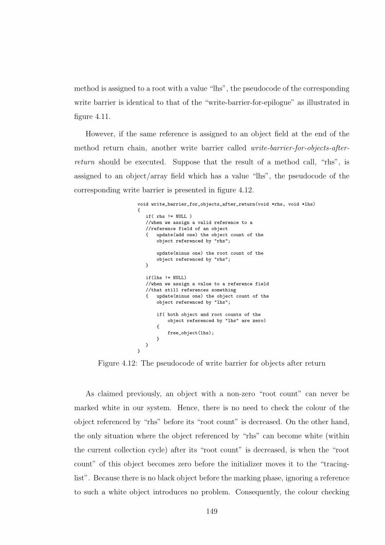
method is assigned to a root with a value “lhs”, the pseudocode of the corresponding

write barrier is identical to that of the “write-barrier-for-epilogue” as illustrated in

figure 4.11.

However, if the same reference is assigned to an object field at the end of the

method return chain, another write barrier called write-barrier-for-objects-after-

return should be executed. Suppose that the result of a method call, “rhs”, is

assigned to an object/array field which has a value “lhs”, the pseudocode of the

corresponding write barrier is presented in figure 4.12.

void write_barrier_for_objects_after_return(void *rhs, void *lhs)

{

if( rhs != NULL )

//when we assign a valid reference to a

//reference field of an object

{ update(add one) the object count of the


update(minus one) the root count of the


}

if(lhs != NULL)

//when we assign a value to a reference field

//that still references something

{ update(minus one) the object count of the


if( both object and root counts of the

object referenced by "lhs" are zero)

{

free_object(lhs);

}

}

}

Figure 4.12: The pseudocode of write barrier for objects after return

As claimed previously, an object with a non-zero “root count” can never be

marked white in our system. Hence, there is no need to check the colour of the

object referenced by “rhs” before its “root count” is decreased. On the other hand,

the only situation where the object referenced by “rhs” can become white (within

the current collection cycle) after its “root count” is decreased, is when the “root

count” of this object becomes zero before the initializer moves it to the “tracing-

list”. Because there is no black object before the marking phase, ignoring a reference

to such a white object introduces no problem. Consequently, the colour checking

149

and related shading operations for the object referenced by “rhs” are not necessary

in this write barrier.

As shown by the above pseudocode, all the write barriers are of O(1) complexity

so their WCETs can be derived and hence, their interference to the user tasks can

be bounded and integrated easily into the WCET analysis of the user tasks. Our

experiments that will be presented in chapter 6 show that none of the barriers’

execution time exceeds 0.33733 microseconds even in the worst case. However,

performing optimizations similar to those proposed in [84] is absolutely desirable

since eliminating unnecessary root related write barriers could significantly improve

the performance of the user tasks running with write barriers (assignments of root

variables are usually very frequent).

Since our system is a preemptive system (see section 4.5), the aforementioned

write barriers can be preempted at any time. If a write barrier is preempted when it

is updating a list used by the collector or updating a reference count, the integrity of

the list and the reference count could be undermined since some other write barriers

may change the list and the reference count before the control can be given back.

In order to make sure that preemptions only happen when all the data structures

used by the collector are in a consistent state, every outmost if branch in the above

write barrier pseudocode must be executed atomically. As will be demonstrated in

chapter 6, the worst-case blocking time introduced by the write barriers is very short

indeed.

4.4 Tracing, Reclamation and Allocation

By running the aforementioned write barriers and therefore continuously updating

the collector’s data structures, user tasks in our system can provide valuable infor-

mation to our garbage collector so that the collector can efficiently find and reclaim

all the acyclic garbage and trace the other objects to identify cyclic garbage. More

150

specifically, the reference counting component processes the “to-be-free-list” and

the “white-list-buffer” to reclaim objects residing in them. On the other hand, the

mark-sweep component traverses the “tracing-list” to identify unreachable objects

and put them into the “white-list-buffer”. As previously discussed in section 4.1,

our hybrid garbage collector should be concurrent so that it can be easily integrated

into many scheduling schemes and schedulability analysis frameworks. Therefore,

both the reference counting component and the mark-sweep component must be

designed to be concurrent. Although it is possible to implement both components

in one task and execute it concurrently with the user tasks, two tasks are actually

used to implement both components separately. This is because the cooperation

and precedence relation between both components can be more easily implemented

with two segregated tasks. In our system, two different GC tasks — the reclaiming

task and the tracing task — are executed concurrently at adjacent priorities.

As previously discussed in section 4.2, an object could be treated by the two

components and consequently the two GC tasks in four different ways. The pro-

posed data structures and write barriers make the system work correctly when both

components consider an object not dead or the reference counting component de-

cides to buffer an object as acyclic garbage before it is identified as garbage by the

mark-sweep component. The solutions to all the other synchronization problems

will be introduced in this section.

First of all, in order to make sure that garbage objects found by both tasks can

be handled correctly, only one task should actually reclaim garbage. It is for this

reason that the “white-list-buffer” is used by the tracing task to buffer the garbage

recognized by the end of each marking phase instead of introducing a real sweeping

phase. Further, in order to ensure that dangling pointers are never introduced by

our collector, the acyclic garbage objects must be reclaimed before those cyclic ones.

This is because reclaiming an acyclic garbage object can never introduce any dan-

gling pointer (since its “object count” is already zero) but reclaiming cyclic garbage

objects could introduce some dangling pointers since they may be still referenced

151

by some other dead objects — acyclic garbage in particular. Consequently, the

processing of the“to-be-free-list” should be given preference over that of the “white-

list-buffer”. In other words, the “white-list-buffer” can only be processed after the

“to-be-free-list” becomes empty.

Whenever the “to-be-free-list” is not empty, the first block of the first object in

the list will be examined by the reclaiming task. If it has any direct child object, the

“object count” of its direct child must be decreased by one and if both the “object

count” and the “root count” are zero, that direct child object will be linked to the

rear of the “to-be-free-list”. Notice that protections similar to those used in our write

barriers must be made again in this case. That is, the aforementioned direct child

must be first unlinked from one of the “tracing-list”, “white-list” and “white-list-

buffer”. Moreover, the “working-pointer” should be adjusted as well, if necessary.

Having processed all its direct children, the current block can be reclaimed and

the next block will be found and processed in the same way until the last block of

the current object is met. The whole procedure repeats from then on until all the

objects in the “to-be-free-list” are reclaimed.

Then, the whole “white-list-buffer” will be moved to a temporary list (involving

only a few memory accesses) and emptied for the future use. As all the objects in the

“white-list-buffer” are garbage identified previously, no further reference can be built

to point to any of them after the last objects were inserted into the current “white-

list-buffer”. If there was a reference pointing to an object when it was added into the

“white-list-buffer”, the reference must be from an object/array already identified by

the tracing tasks as garbage (and therefore already put into the “white-list-buffer”)

or buffered in the “to-be-free-list” (otherwise, the referenced object should be found

alive by our tracing task). Consequently, after the “to-be-free-list” becomes empty,

all the objects that could potentially reference a dead object in that temporary list

from outside have been reclaimed. Since it is impossible to build any new reference to

a dead object, those dead objects in the temporary list can now be safely reclaimed,

one by one without any attempt to process their children.

152

If new objects are inserted into the “to-be-free-list” during the processing of

the above temporary list, the reclaiming task will continue to process the “to-be-

free-list” after the work on the temporary list is done. Otherwise, if the “white-

list-buffer” is not empty, it will be moved to the above temporary list again and

procedure repeats until both lists are empty. Then, the reclaiming task will have

nothing to do and therefore suspend itself. The pseudocode of the reclaiming task

can be found in figure 4.13.

In order to protect the integrity of the collector’s data structures, at least the

processing of each field in the reclaiming task must be performed atomically. Be-

cause, in most cases, the “to-be-free-list” can only be accessed by the reclaiming task,

there is no need to protect the objects in that list except the last one which could

be accessed by the write barriers. Moreover, linking any object into the “free-list”

must be atomic. Otherwise, the free list may be destructed.

One thing needs to be noticed is that the “object count” of an object could be

overestimated. Suppose that an object is referenced by a cyclic data structure and

dies after the other parts of that structure are reclaimed. Since cyclic garbage is

not examined to update the information of its children, the “object count” of the

aforementioned object will be overestimated. This is not a problem because:

1. The objects with overestimated reference counts can be identified as garbage

by the tracing task after they die.

2. These objects are already considered as a part of the cyclic structure when we

perform static analyses (see chapter 5).

The tracing task starts by moving all the objects in the “tracing-list” to the

empty “white-list”. This is a very efficient operation only involving several reference

assignments. Afterwards, the “white-list” will be traversed so that all the objects

directly referenced by roots (i.e. objects with “root counts” greater than zero) can

be moved back to the “tracing-list” and all the other objects can be marked white.

153

void Reclaiming_work(){

while(true)

{

while( ‘‘to-be-free-list’’ is not empty || ‘‘white-list-buffer’’ is not empty )

{

while( ‘‘to-be-free-list’’ is not empty )

{

void * temp = the address of the first object in the ‘‘to-be-free-list’’;

update the head of the ‘‘to-be-free-list’’;

get the type information for the object referenced by ‘‘temp’’;

set the first user word of the object referenced by ‘‘temp’’ as the

the next word to be processed --- ‘‘nword’’;

while( there is still some user reference field not yet processed in the

object referenced by ‘‘temp’’ )

{

int block_offset = the offset of ‘‘nword’’ within its containing block;

if( ‘‘nword’’ is a reference field )

{

get the value of ‘‘nword’’ by using ‘‘temp’’ and ‘‘block_offset’’;

if( ‘‘nword’’ is not null)

{

update(minus one) the object count of the object referenced by

"nword";

if( both reference counts of the object referenced by "nword"

are zero)

{

unlink the object referenced by "nword" from its current list;

add it to the "to-be-free-list";

}

}

}

update ‘‘nword’’ to be the next word.

if( all the fields in the block identified by ‘‘temp’’ have

been processed )

{

update ‘‘temp’’ to point to the next block;

reclaim the block identified by ‘‘temp’’;

}

}

reclaim all the remaining blocks of the object referenced by ‘‘temp’’;

}

move the whole ‘‘white-list-buffer’’ to the ‘‘cyclic-garbage-list’’;

empty the ‘‘white-list-buffer’’;

while( the ‘‘cyclic-garbage-list’’ is not empty )

{

void * temp = the address of the first object in the ‘‘cyclic-garbage-list’’;

update the head of the ‘‘cyclic-garbage-list’’;

for( each block within the object referenced by ‘‘temp’’)

{

update ‘‘temp’’;

reclaim the current block;

}

}

}

wait for either the ‘‘to-be-free-list’’ or the ‘‘white-list-buffer’’ to be filled

again;

}

}

Figure 4.13: The pseudocode of the reclaiming task

154

If an object’s “root count” becomes non-zero after it is initialized white, it should be

moved to the “tracing-list” by a root related write barrier when its “root count” is

increased to one. If an object’s “root count” becomes non-zero before it is examined

by the initializer, there will be no difficulty for the initializer to move that object

into the “tracing-list”. Consequently, objects directly referenced by roots can never

be marked white during the initialization phase. Since marking can never turn those

objects back to white, objects directly referenced by roots can never be marked white

during any collection cycle either.

Since the initialization phase could be preempted by the user tasks, a write

barrier could be fooled by the temporary colour of objects. If the user tasks require

to build a reference to an object (given that this object is not referenced by any

root) which has not yet been marked white, the corresponding write barrier will not

recognize the white object and will not move it to the “tracing-list” although it is

logically white indeed. This is not going to be problem because there is not any

black object before marking begins and therefore the strong tri-colour invariant still

holds.

By the end of the initialization phase, all the objects directly referenced by roots

are already in the “tracing-list” and all the objects left in the “white-list” have been

marked white. Marking begins by setting the “working-pointer” to point to the

head of the “tracing-list”. The tracing task then finds all the direct children of that

object and moves any of them with white colour to the end of the “tracing-list”

(implicitly marked grey). Next, the “working-pointer” is going to be advanced to

point to the next object in the “tracing-list” and consequently, the current one will

be implicitly marked black. Such a procedure repeats until the “working-pointer”

becomes null (after the last object in the “tracing-list” is scanned). In other words,

the marking phase completes when there is not any grey object left. Finally, all the

objects left in the “white-list” are garbage. The tracing task links all of them to

the end of the “white-list-buffer” and suspends itself until the next collection cycle.

The pseudocode of the tracing task can be found in figure 4.14.

155

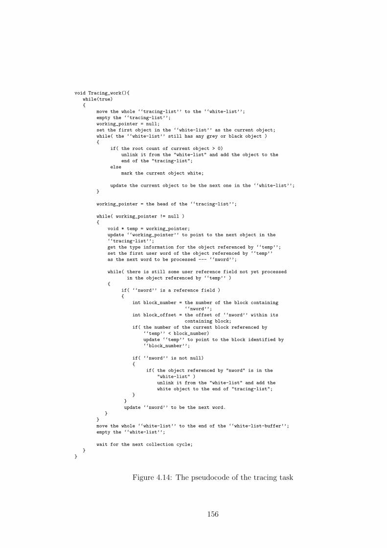
void Tracing_work(){

while(true)

{

move the whole ‘‘tracing-list’’ to the ‘‘white-list’’;

empty the ‘‘tracing-list’’;

working_pointer = null;

set the first object in the ‘‘white-list’’ as the current object;

while( the ‘‘white-list’’ still has any grey or black object )

{

if( the root count of current object > 0)

unlink it from the "white-list" and add the object to the

end of the "tracing-list";

else

mark the current object white;

update the current object to be the next one in the ‘‘white-list’’;

}

working_pointer = the head of the ‘‘tracing-list’’;

while( working_pointer != null )

{

void * temp = working_pointer;

update ‘‘working_pointer’’ to point to the next object in the

‘‘tracing-list’’;


set the first user word of the object referenced by ‘‘temp’’

as the next word to be processed --- ‘‘nword’’;

while( there is still some user reference field not yet processed

in the object referenced by ‘‘temp’’ )

{


{

int block_number = the number of the block containing

‘‘nword’’;

int block_offset = the offset of ‘‘nword’’ within its

containing block;

if( the number of the current block referenced by

‘‘temp’’ < block_number)

update ‘‘temp’’ to point to the block identified by

‘‘block_number’’;


{

if( the object referenced by "nword" is in the

"white-list" )

unlink it from the "white-list" and add the

white object to the end of "tracing-list";

}

}


}

}

move the whole ‘‘white-list’’ to the end of the ‘‘white-list-buffer’’;

empty the ‘‘white-list’’;

wait for the next collection cycle;

}

}

Figure 4.14: The pseudocode of the tracing task

156

As proved previously, the reference counting component has no difficulty of re-

claiming any object, the scanning of which has not been performed at all or has

been completed. However, what if an object is being scanned while the reclaiming

task intends to reclaim it? Suppose that a user task preempts the tracing task while

it is scanning an object, it is possible that the (acyclic) object under scan dies and

is consequently linked to the “to-be-free-list” during the execution of the user task.

If the data structures (i.e. the “tracing-list” and “working-pointer”) are correctly

updated and the control is immediately given back to the tracing task after the

user task finishes, there will be no problem to resume the scan. However, if the

reclaiming task recycled that object before the control is given back to the tracing

task, the tracing task will be unable to resume the preempted scan as the blocks

may have already been initialized and used by other objects. Therefore, we pro-

pose to scan at least each field atomically and perform a checking before every time

a field can be fetched so that if the current object has been reclaimed during the

time when the tracing task was preempted, the tracing task can skip the current

object and continue its execution without any problem. More specifically, an object

must be protected by marking the “M” field in its header (see figure 4.7) when it

is being scanned. The reclaiming task checks that field in the object header before

that object can be reclaimed. If such a field is set, a global variable must be set to

inform the tracing collector that the object currently under scan will be reclaimed

so that the scanning of the current object can be safely quit. Then, the above global

variable can be reset so the tracing task can proceed again.

The allocator in our system can be as simple as tracing the “free-list” for the

requested number of blocks and updating the head of the list to the new position. In

addition, it should block the execution of the current task (before actually traversing

the “free-list”) if there is not enough memory1. It should also log, at the beginning

of the allocation, the amount of free memory that would be available after this

allocation so that the requested number of blocks can be secured even if the allocator

1 Guarantees can be provided to ensure that such blocking never happens. See chapter 5.

157

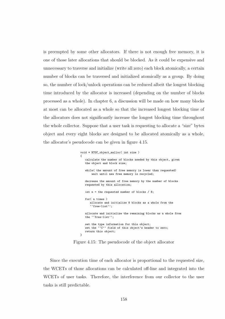
is preempted by some other allocators. If there is not enough free memory, it is

one of those later allocations that should be blocked. As it could be expensive and

unnecessary to traverse and initialize (write all zero) each block atomically, a certain

number of blocks can be traversed and initialized atomically as a group. By doing

so, the number of lock/unlock operations can be reduced albeit the longest blocking

time introduced by the allocator is increased (depending on the number of blocks

processed as a whole). In chapter 6, a discussion will be made on how many blocks

at most can be allocated as a whole so that the increased longest blocking time of

the allocators does not significantly increase the longest blocking time throughout

the whole collector. Suppose that a user task is requesting to allocate a “size” bytes

object and every eight blocks are designed to be allocated atomically as a whole,

the allocator’s pseudocode can be given in figure 4.15.

void * RTGC_object_malloc( int size )

{

calculate the number of blocks needed by this object, given

the object and block size;

while( the amount of free memory is lower than requested)

wait until new free memory is recycled;

decrease the amount of free memory by the number of blocks

requested by this allocation;

int n = the requested number of blocks / 8;

for( n times )

allocate and initialize 8 blocks as a whole from the

‘‘free-list’’;

allocate and initialize the remaining blocks as a whole from

the ‘‘free-list’’;

set the type information for this object;

set the ‘‘C’’ field of this object’s header to zero;

return this object;

}

Figure 4.15: The pseudocode of the object allocator

Since the execution time of each allocator is proportional to the requested size,

the WCETs of those allocations can be calculated off-line and integrated into the

WCETs of user tasks. Therefore, the interference from our collector to the user

tasks is still predictable.

158

4.5 Scheduling

As proposed in chapter 3, one of our new real-time garbage collector design criteria

is to integrate garbage collection into more advanced real-time scheduling schemes

without any significant change to the original scheduling algorithm, task model or

analysis. However, the garbage collector should not limit itself to a specific schedul-

ing scheme ruling out the opportunities for other improvements. Consequently, it

would be preferable to design the scheduling of our garbage collector in two steps.

First, the garbage collector should be integrated with a task model that is generic

to most real-time systems. Second, the collector should be integrated into a specific

real-time scheduling scheme chosen or developed for the target system (according

to the overall requirements of the whole system). Because the garbage collector has

been designed to be compatible with the most common real-time task model in the

first step, there should be no difficulty when integrating the garbage collector into

the given real-time scheduling scheme. More importantly, based on the same reason,

choosing another real-time scheduling scheme for the system will be very unlikely to

fundamentally change the design of our garbage collector. As periodic hard real-time

tasks are the most common tasks in real-time systems and most real-time schedul-

ing schemes support this task model, our garbage collector should be designed as

periodic tasks (recall that our garbage collector is composed of two tasks).

4.5.1 Making GC Tasks Periodic

Because mark-sweep collectors are naturally performed in cycles and the worst-case

lengths of collection cycles in each application are stable (which are usually functions

of heap size or maximum amount of live memory), it is relatively easy to make them

periodic. As discussed in section 4.4, our tracing task suspends itself after every

time objects in the “white-list” are dumped into the “white-list-buffer” but it is not

clearly defined when the next collection cycle begins. In order to make the tracing

task periodic, a period must be associated with it so that only one collection cycle

159

can be performed in each period. After the tracing task suspends itself, it waits

for its next period. The real issue of making a tracing garbage collector periodic

is how to guarantee that the real-time user tasks never run out of memory, given

the collector’s period. Robertz and Henriksson have given an analysis of the overall

memory usage and the collector’s period (deadline equals period) in [87] but there

is unsurprisingly no consideration of a potential reference counting partner. Our

analysis of the overall memory usage and the hybrid garbage collector’s period (and

also the deadline) will be introduced in chapter 5.

By contrast, the reclaiming task is always ready to run except when both the

“to-be-free-list” and the “white-list-buffer” are empty at the same time so it has

no garbage to reclaim. Because the time taken to reach such a situation is very

unpredictable and unstable, associating a specific period with the reclaiming task

can be very hard. However, all garbage objects need not be reclaimed only if the

amount of memory already reclaimed can satisfy all the memory requirements even

in the worst case. Therefore, it is possible to associate a period and a “work-amount”

limit within each period with the reclaiming task so that whenever the reclaiming

task has done enough work, it suspends itself and waits for the next period. Since

a “work-amount” limit has been set for the reclaiming task during each period, the

WCET of each release of our reclaiming task can be estimated (see chapter 5). In

addition, such a “work-amount” limit must be large enough so that we can still

ensure that the user tasks are never blocked by the collector due to the lack of free

memory (see chapter 5).

The amount of work performed by the reclaiming task can be stated as either

the computation time or the number of blocks reclaimed. Although the two metrics

are equivalent in the worst case, choosing different metrics can still give the system

different behaviours, particularly when the computation time of the reclaiming task

is underestimated. More details of this issue will be discussed in the next chapter.

Currently, we measure the work amount in terms of the number of blocks re-

claimed. Whenever the number of blocks reclaimed by the reclaiming task in the

160

current period reaches its limit, the reclaiming task should suspend itself and wait for

the next period (the “work-amount” limit will be reset in the next period). How-

ever, an optimization can be performed to better utilize the processor resources.

Instead of suspending itself when the “work-amount” limit is reached, the reclaim-

ing task should continue its execution as a background task until its next period.

From any user task’s point of view, this is generally equivalent to suspending the

reclaiming task when enough work has been done because all the user tasks can

preempt the reclaiming task executed at background within a small bounded time

which is already a part of the blocking factors of our user tasks. Moreover, if the

amount of garbage is not enough for the reclaiming task to reach its “work-amount”

limit in one period, the reclaiming task will never go to the background during that

period. Since the actual execution time of a starved release of the reclaiming task

can never be higher than that of a release which reaches the “work-amount” limit,

the worst-case interference from the reclaiming task to other tasks is not changed.

In order to obtain lower GC granularities, the reclaiming task should always be

given preference over the tracing task. Therefore, when there is any garbage, the

reclaiming task can respond quickly to reclaim it rather than waiting until a release

of the tracing task finishes. For simplicity, it is required that both the tracing and

the reclaiming tasks should have the same period (deadline equals period) so their

priorities are adjacent (given that the priorities are determined according to either

DMPO or RMPO). We call such a period and deadline the GC period and the GC

deadline respectively.

Also notice that although the priority of the reclaiming task is usually higher than

that of the tracing task, the tracing task could still end with acyclic garbage in both

the “white-list” and the “white-list-buffer”. This is because the reclaiming task has

a “work-amount” limit for each release and therefore some acyclic garbage objects

may be left in the “white-list” albeit they are reachable from the “to-be-free-list”. If

such garbage is not scanned before reclamation, its children’s reference counts will

be overestimated so the behaviour of the whole system will be unpredictable (such

161

objects’ direct children may be not a part of any cyclic structure so if those children

can only be recognized by the tracing task due to the overestimated reference counts,

the analysis in the next chapter will become inadequate). As proved previously,

this is not going to happen in our system because the “to-be-free-list” is always

processed before the “white-list-buffer”. Moreover, scheduling the reclaiming task

periodically does not influence the aforementioned property since it will not change

the processing order of the two lists.

4.5.2 Scheduling GC Tasks

Since both the tracing task and the reclaiming task are designed as periodic tasks, it

should be relatively easy to integrate them into most real-time systems. In particu-

lar, if a real-time system is only composed of periodic hard real-time user tasks, the

standard fixed priority preemptive scheduling scheme will be sufficient. However,

as discussed previously, many real-time applications consist of a mixture of periodic

hard real-time tasks, sporadic hard real-time tasks and aperiodic soft or non-real-

time tasks running on the same processor. On the one hand, the timing constraints

related to the hard real-time tasks and the mandatory components must be obeyed.

On the other hand, the overall system utility, functionality and performance must

be maximized. The most common but efficient way to satisfy this requirement is

to use a bandwidth preserving algorithm to schedule the whole system so that the

impacts on the hard real-time tasks can still be kept under control while the optional

components along with the tasks other than the hard real-time ones can get as much

resources as possible at their earliest possible time.

As introduced in section 3.3, there are three sources of spare capacity in a real-

time system. While all the bandwidth preserving algorithms can reclaim extra

capacity and make it available at high priorities for the tasks other than the hard

real-time ones, only a few of them can reclaim both gain time and spare time as

high priority resources. The dual-priority scheduling algorithm proposed by Davis

162

[36] is the most straightforward but fairly efficient one of those algorithms that can

reclaim all kinds of spare capacity. Moreover, it is based on fixed priority preemp-

tive scheduling so plenty of platforms can be used to implement this algorithm.

Therefore, we choose the dual-priority scheduling scheme for our garbage-collected

flexible real-time system (however, the choice is not limited to this algorithm as our

collector is composed of periodic tasks which are supported by virtually all real-time

scheduling schemes). In such a system, a set of periodic and sporadic real-time user

tasks with hard timing constraints coexists with some aperiodic soft- or non-real-

time user tasks along with our periodic tracing and reclaiming tasks which have

hard timing constraints as well. In order to discuss the scheduling algorithm, the

task model must be defined in more detail.

1. Priorities are split into three bands: Upper, Middle and Lower [36]. Any

priority in a higher priority band is higher than those in the lower priority

bands.

2. Hard real-time tasks (including both user and GC tasks) are released either

periodically or sporadically and executed in either the lower or upper band.

3. Each periodic hard real-time user task has a deadline which is not greater than

its period.

4. Each sporadic hard real-time user task has a deadline which is not greater

than its minimum inter-arrival time.

5. Soft- or non-real-time tasks are released aperiodically and their priorities are

always within the middle band.

6. Soft- or non-real-time tasks neither produce any cyclic garbage nor allocate

memory from the heap. This rigid restriction will be relaxed in chapter 7.

7. Each task executes at its own priority (or priorities).

163

In the dual priority scheduling algorithm, a hard real-time task can have two

priorities at different stages, one in the upper and one in the lower band. Upon

a hard real-time task’s release, it executes at its lower band priority and so gives

preference to the soft or non-real-time tasks in the middle band. However, in order to

guarantee that all the hard timing constraints can be met, each hard real-time task’s

release should be given an appropriate promotion time. When the given promotion

time has elapsed, the hard real-time task is promoted to its higher band priority

and therefore preempts any soft- or non-real-time task still executing. Then, the

hard real-time task will only suffer from interference from those hard real-time tasks

that have higher priorities (within the upper band) until the next release when its

priority is degraded to the lower band again.

The promotion time for each task must not be too late, which means that every

hard real-time task must stay in the upper priority band for a long enough time

during each release so that it can meet its deadline. Assuming, in the worst case, all

the hard real-time tasks are promoted to the upper priority band at the same time,

the worst-case response time wi (from the promotion time rather than the release

time) of the hard real-time task i can be estimated with the standard response time

analysis [6] since tasks other than the hard real-time ones cannot influence the hard

real-time tasks’ execution (assuming they are executed independently). Hence, if a

promotion delay Yi is defined as the difference between a promotion time and its

corresponding release time (both are absolute time), Yi + wi must be less than the

corresponding deadline Di. Therefore, the maximum value of Yi can be represented

as Di −wi where wi is estimated as if all the tasks are scheduled in a standard fixed

priority system. On the one hand, extra capacity can be reclaimed at an earlier time

for the soft- or non-real-time tasks. If all the hard real-time tasks are running at

lower band priorities or suspended for the next period or blocked for some reason,

the soft- or non-real-time tasks can run until a task is ready at an upper band

priority. On the other hand, the hard real-time deadlines are still guaranteed to be

met.

164

In the dual-priority scheduling scheme, gain time can also be identified and

reused for the soft- or non-real-time tasks. If some task does not execute as long as

its WCET and there is neither a soft- nor a non-real-time task pending, the gain time

may be reused by a hard real-time task running at a lower band priority. If a hard

real-time task executes for an interval of ∆t before its promotion time has elapsed,

the promotion time can then be extended by at most ∆t without jeopardising the

timing constraints. In other words, the hard real-time tasks “borrow” the gain time

and use them at lower band priorities but whenever a soft- or non-real-time task

requires to execute, they try their best to return the gain time they used by delaying

the promotion time. Moreover, if some other mechanisms can be used to identify

gain time gi before promoting task i, it will be safe to extend the corresponding

promotion time by gi.

If a sporadic task arrives at its highest rate, it will be scheduled as if it is a

periodic task which has a period equal to its minimum inter-arrival time. Otherwise,

if the earliest next release time of the sporadic hard real-time task i after time t is

represented as xi(t), the next promotion time will be xi(t) + Yi. If task i is not

ready at a promotion time, the next promotion time can be calculated and no task

is promoted this time. Therefore, soft- or non-real-time tasks can reuse such spare

time for their benefits.

Applying this technique to our GC tasks only needs a few trivial modifications

to the original algorithm. First, both the reclaiming and the tracing tasks are

considered as a whole and the promotion time is defined as the release time add the

difference between the deadline (deadline equals period) and the worst-case response

time of the tracing task. Secondly, instead of giving arbitrary priorities to hard real-

time tasks in the lower band, it is required to maintain the same priority order of

hard real-time tasks in both the upper and the lower bands. The above requirements

are introduced to make sure that the reclaiming task always has a higher priority

than the tracing task (in either band) before it finishes its compulsory work. This

is essential for the WCET estimation of our tracing task (see chapter 5). As the

165

reclaiming task finishes its compulsory work, it goes to the lowest priority in the

lower band (i.e. the background priority which is not used by any user task) and

returns to its original lower band priority upon the next release of the tracing task.

Now, our approach can only ensure that both the reclaiming and the tracing

tasks get enough system resources in each period of them. To guarantee that the

real-time tasks with higher priorities than the reclaiming task (within the same

band) can never be blocked because of the lack of free memory, we require that the

reclaiming task should always try to reserve enough free memory, Fpre, for those

high priority tasks (see chapter 5). When the reclaiming task is running at an

upper band priority, this can be guaranteed by our static analysis as will be seen

in chapter 5. However, before the promotion time, if the amount of free memory

becomes lower than Fpre, the priorities of both the reclaiming and the tracing tasks

should be promoted. Otherwise, they should be executed at their original priorities

until the promotion time.

Another approach we use to reclaim spare capacity is to set a lower limit on

the reclaiming task’s work amount if, in the previous tracing period, the reclaiming

task did any extra work. As discussed previously, instead of suspending itself, the

reclaiming task goes to the background priority after finishing all its compulsory

work (in the current period). Hence, it is possible that some extra work Ei (within

the period i) is done by the reclaiming task before the next period. Consequently,

the “work-amount” limit of the next release of the reclaiming task can be reduced

by Ei at the end of the current period. If the initially specified (off-line) “work-

amount” limit for each period and the actual (online) “work-amount” limit for the

period i are denoted as C and Ci respectively, Ci can then be calculated at the

very beginning of the period i as Ci = C − Ei−1. The reclaiming task may do less

work at its upper band priority in its period i so soft- or non-real-time tasks could

benefit. In addition, such spare capacity can even be reclaimed earlier by extending

the promotion time of our GC tasks (period i) by the WCET of reclaiming Ei−1

blocks at the beginning of their release (this feature has not been realized in the

166

current implementation). This is safe because the worst-case response time of the

release i of our tracing task is also reduced by at least the WCET of reclaiming Ei−1

blocks. Notice, Ei, C and Ci are all measured in number of blocks in the current

implementation but there is no difficulty to follow the same approach to reclaim

spare capacity when they are all measured in execution time.

Finally, we are going to justify that designing our garbage collector as periodic

tasks is not only a requirement of easy integration with different scheduling frame-

works but also a reflection of the nature of garbage collection. Essentially, garbage

collection is a system service, the main purpose of which is to provide enough mem-

ory for the user tasks. Performing the garbage collection work aggressively to reclaim

more than enough memory may not significantly benefit the whole system. In ad-

dition, the responsiveness of a garbage collector is not of great importance unless

it is not responsive enough to satisfy the user tasks’ requirements within tolerable

delays. Hence, designing our garbage collector as periodic hard real-time tasks and

introducing them into bandwidth preserving algorithms such as the dual-priority

scheduling algorithm reflect the nature of garbage collection as well. One thing

worth special mentioning is that the user tasks’ memory requirements could be ei-

ther “hard” or “soft”. Does the collector need to do enough work and be responsive

enough to satisfy both “hard” and “soft” requirements? In our system, the garbage

collector guarantees to reclaim enough memory for both “hard” and “soft” memory

requirements but only the “hard” memory requirements are ensured to be satisfied

without blocking. A “soft” memory requirement, on the other hand, is only guar-

anteed to be satisfied within a relatively long but still bounded time. More details

of this issue will be discussed in chapter 7.

4.6 Summary

In this chapter, a new garbage collection algorithm along with a new scheduling

scheme for garbage-collected real-time systems were presented. The new garbage

167

collection algorithm is developed according to our new design criteria from the very

beginning. It is believed that all the operations related to our garbage collector

(e.g. memory access, write barriers, allocations, tracing task, reclaiming task and

so on) are bounded and short in terms of execution time. Moreover, the worst-case

interference from our garbage collector and write barriers to the user tasks can also

be predetermined. Experimental supports for such claims can be found in chapter

6. By running a mark-sweep collector and maintaining exact root information, our

garbage collector is able to reclaim all the garbage and never misunderstand any

word in memory. As root scanning and object copying are totally eliminated in

our new algorithm, all the atomic operations in our system are of O(1) complexity

and therefore bounded so that predictable preemptions can be achieved. Experi-

ment results that will be presented in chapter 6 can prove that such preemptions

are not only predictable but also fast. Graceful degradation is also a feature of our

new algorithm as both reference counting and mark-sweep algorithms can correctly

proceed even when there is not any free memory. The worst-case granularity of our

reference counting component is definitely small enough. However, it is not clear

how the negative effect of the high granularity mark-sweep component can be eased.

More discussions on the overall memory usage of our hybrid system will be given in

chapter 5. Finally, our garbage collector is integrated into an advanced scheduling

scheme (which reclaims all kinds of spare capacity) without any significant modifica-

tion to the original scheduling algorithm, task model and analysis. It is also possible

to easily integrate our garbage collector into another scheduling scheme that also

supports periodic tasks.

If our garbage collector is used under a purely sporadic workload, it will treat all

the sporadic tasks as periodic tasks with the minimum inter-arrival times as their

periods. In such a case, spare capacity (including the spare capacity caused by

our garbage collector) can be reclaimed by the dual-priority scheduling algorithm.

Although our garbage collector cannot work with a purely aperiodic workload, such

tasks can still be deployed along with periodic or sporadic tasks if they do not

168

influence the memory usage of those periodic and sporadic tasks (see section 4.5.2

and chapter 7).

Notice that intensive use of large data (either objects or arrays) under a small

block size configuration can dramatically increase the overheads of our algorithm in

both temporal and spatial aspects. Therefore, different applications should choose

different block sizes to satisfy their requirements. However, even a single application

could have extremely small and large data in which case, choosing a unique block

size to build an efficient application becomes more difficult. Although it is possible

to use different block sizes for large and small data respectively, fragmentation may

become a problem again.

169

Chapter 5

Static Analysis

A new hybrid garbage collection algorithm has been introduced in chapter 4 along

with its scheduling scheme. However, it was not clear how the negative effect of

the high GC granularity mark-sweep component can be modeled and eased. It was

also not clear how to achieve the important parameters such as the WCETs and the

period of the GC tasks, the amount of memory reserved to synchronize the reclaiming

task and the high priority user task allocations as well as the “work-amount” limit

imposed on the reclaiming task. More importantly, how to provide both temporal

and spatial guarantees has not been discussed as well. In this chapter, all the above

issues will be addressed by performing a static analysis to characterize our user

tasks, derive the worst-case response times and secure all the memory requests.

Previous work such as [87, 60] has demonstrated how a pure tracing hard real-

time system can be analyzed in terms of both timing constraints and memory

bounds. However, our hybrid garbage collector has some unique features that cannot

be modeled by the previous research results. Further, the task model and scheduling

approach adopted are also different from those in the previous work. Therefore, a

new static analysis must be developed for our system to derive the required param-

eters and provide both temporal and spatial guarantees.

170

5.1 Notation Definition and Assumptions

First of all, a summary of notations used in this chapter is given in table 5.1. Detailed

explanations will be provided for some of these notations later.

By using such notations, some formulae can be derived to formally describe the

memory usage of the whole system. They also reveal the relations between some

of the notations and therefore enable a better understanding of these notations.

More importantly, they will also be used in other parts of this chapter to derive the

formulae that are used to derive the required parameters.

It is widely accepted that a garbage-collected heap without the fragmentation

issue is only composed of live memory, free memory and garbage that has not been re-

claimed. In our system, garbage consists of both cyclic garbage and acyclic garbage.

Notice, acyclic objects referenced by cyclic structures can also become a part of the

cyclic garbage. On the one hand, the reclaiming task has no difficulty in identifying

all the acyclic garbage that emerged during a GC period before the end of that pe-

riod, although it may require extra time to reclaim all such garbage. On the other

hand, not all the cyclic garbage can be identified by the tracing task within the

GC period where the garbage emerges. However, all such floating cyclic garbage

is guaranteed to be identified by the end of the next GC period. Thus, the only

garbage that cannot be identified by the end of a GC period is the floating cyclic

garbage that emerged in this GC period. Further, not all the garbage identified

can also be reclaimed by the end of a GC period. The amount of already identified

garbage that still exists at the beginning of the next GC period, i + 1, is Gi −GRi.

Therefore, the heap composition at the very beginning of the GC period i + 1 can

be given as below:

H = Li+1 + Fi+1 + FCGi + Gi − GRi (5.1)

Intuitively, the amount of allocated (non-free) memory at time t is the difference

171

Symbols Definitions

aj the maximum amount of memory allocated by any one release of the hard real-time user task j

Ai the amount of allocated (non-free) memory at the very beginning of the ith GC period

AGGi the amount of acyclic garbage that emerges during the ith GC period

B the worst-case blocking factor caused by garbage collection

Cj the worst-case execution time of the hard real-time user task j

Creclaiming the worst-case execution time of the reclaiming task

Ctracing the worst-case execution time of the tracing task

cggj the maximum amount of cyclic garbage introduced by any one release of the hard real-time user task j

CGGi the total amount of cyclic garbage that emerges during the ith GC period

CGGmax the maximum amount of cyclic garbage that emerges during any GC period

D the GC deadline and also the GC period

Dj the deadline of the hard real-time user task j

Fi the amount of free memory at the very beginning of the ith GC period

Fpre the amount of free memory the system should reserve for the user tasks with higher priorities than the

reclaiming task (promoted)

Fmin the minimum amount of free memory at the very beginning of any GC period

FCGi the amount of floating cyclic garbage that emerges during the ith GC period

Gi the total amount of garbage that can be recognized at the end of the ith GC period

GRi the total amount of garbage reclaimed during the ith GC period

H the size of the heap

hp(j) the set of all the users tasks with higher priorities than the user task j (all promoted)

hp(GC) the set of all the users tasks with higher priorities than the GC tasks (all promoted)

IR the longest time needed by the tracing task to initialize an object

Li the amount of live memory at the very beginning of the ith GC period

Lmax the upper bound of live memory consumption of the whole system

maxLj the maximum amount of live memory of the hard real-time user task j

NEWi the total amount of new memory allocated during the ith GC period

NEWmax the maximum amount of new memory allocated during any GC period

NOI the maximum number of objects that occupy H − Fpre heap memory. This is also the worst-case number

of objects that any release of the tracing task needs to initialize

P the set of hard real-time user tasks in the whole system

Rj the worst-case response time of the hard real-time user task j

Rpre the worst-case response time of the reclaiming task (promoted) to reclaim as much memory as the user

tasks allocate during that time

Rreclaiming the worst-case response time of the reclaiming task

Rtracing the worst-case response time of the tracing task

RR the time needed to reclaim one unit of memory in the worst case

Tj the period or the minimum inter-arrival time of the hard real-time user task j

TR the time needed to trace one unit of memory in the worst case

Yj the longest possible promotion delay of the hard real-time user task j

Ygc the specified promotion delay of all the GC tasks

Y ′

gc the longest possible promotion delay of all the GC tasks

Table 5.1: Notation definition

172

between the heap size and the amount of free memory also at time t. Thus, the

amount of allocated (non-free) memory at the very beginning of the i + 1th GC

period can be represented as Ai+1 = H − Fi+1. Consequently, the equation 5.1 on

page 171 can be rewritten as:

Ai+1 = Li+1 + FCGi + Gi − GRi (5.2)

By the end of the GC period i, all the acyclic garbage and a part of the cyclic

garbage that emerged within that period can be recognized. For those garbage

objects that emerged before the GC period i, either they have been reclaimed or

otherwise they are going to be identified by the end of the GC period i. Thus, Gi

can be further decomposed as:

Gi = AGGi + CGGi − FCGi + FCGi−1+Gi−1 − GRi−1

for i ≥ 1 (5.3)

G0 = AGG0 + CGG0 − FCG0 (5.4)

where GC period 0 is the first GC period in our system. As it is supposed that

there is not any garbage before the first GC period, equation 5.4 does not include

any previous garbage.

The accumulation (which could be negative) of live memory during the GC period

i is the difference between the amount of new memory allocated and the amount

of garbage that emerges during that period. As garbage can be either acyclic or

cyclic, the accumulation of live memory during the GC period i can be denoted as

NEWi − AGGi − CGGi. Therefore, we get:

Li+1 = Li + NEWi − AGGi − CGGi (5.5)

173

On the other hand, the accumulation (which could be negative as well) of al-

located (non-free) memory during the GC period i is the difference between the

amount of new memory allocated and the amount of garbage reclaimed during that

period. Thus, the amount of allocated (non-free) memory at the very beginning of

the GC period i + 1 can be represented as:

Ai+1 = Ai + NEWi − GRi (5.6)

For simplicity but without loss of generality, several further assumptions (in

addition to those made in the subsection 4.5.2 when our task model was defined)

are made for the analysis that will be discussed in this chapter.

1. The context-switching overheads are negligible.

2. All the hard real-time user tasks are completely independent of each other,

which suggests that the only reason for a user task to get blocked is the lack

of free memory.

3. The user tasks do not suffer from any release jitter, which is the maximum

release time variations.

4. The priorities are assigned according to DMPO (deadline monotonic priority

ordering).

5.2 The Period and Deadline of the GC Tasks

In order to guarantee that the user tasks always have enough free memory to allocate,

the amount of free memory available at the beginning of the GC period i must not

be less than the accumulation of allocated memory during that period. However,

because the exact amount of accumulation of allocated memory during each GC

period is hard to obtain, it is required that the amount of free memory at the

174

beginning of any GC period should never be less than the maximum accumulation

of allocated memory during any GC period. This is to be explored below:

Minimum Free Memory Requirement

Assuming, in the worst case, that Li equals Lmax, since Li+1 must not be greater

than Lmax, we get Li+1 − Li ≤ 0. Applying equation 5.5 on page 173 to this gives:

NEWi − AGGi − CGGi ≤ 0 (5.7)

and therefore,

NEWi − AGGi ≤ CGGi (5.8)

From equation 5.6 on the preceding page, we get:

Ai+1 − Ai = NEWi − GRi (5.9)

If the value of GRi is not smaller than that of NEWi, there will be no accumu-

lation of allocated memory at the end of GC period i. As discussed in chapter 4, an

upper bound on the value of GRi should be set. The initial value of such an upper

bound for each GC period is set to NEWmax since by reclaiming NEWmax garbage,

Ai+1−Ai is already guaranteed not to be greater than zero. Positive accumulation of

allocated memory can only happen when GRi < NEWi. In the worst scenario, the

reclaiming task only reclaims acyclic garbage during a GC period and the amount of

such garbage is less than the total amount of allocations performed in that period.

That is, GRi = AGGi and AGGi < NEWi. Thus, in the worst case,

Ai+1 − Ai = NEWi − AGGi (5.10)

Applying inequality 5.8 to the above equation, we can get:

175

Ai+1 − Ai ≤ CGGi ≤ CGGmax (5.11)

which means that if the GC tasks can provide as much free memory as CGGmax

at the beginning of any GC period, the accumulation of allocated memory at the

end of that GC period can always be satisfied (given that the GC tasks always do

enough work and meet their deadline). In a pure tracing system such as the one

discussed in [87], the collector may be unable to reclaim any garbage at all by the

end of a GC period (all the dead objects are floating) so the maximum accumulation

of allocated memory is identical to the maximum amount of allocations during any

GC period. Thus, free memory as much as the maximum amount of allocations

during any GC period should be made available at the beginning of any GC period.

By contrast, our requirement CGGmax is usually much smaller.

Since enough free memory (CGGmax) has been reserved for all the cyclic garbage

that could emerge within a GC period, we can assume that our GC tasks only

process acyclic garbage during a GC period. Therefore, equation 4.1 on page 121

can be used to model the synchronization between the reclamations and allocations

in our system. That is, free memory as much as Fpre must be reserved for the

user tasks with higher priorities than the reclaiming task (promoted) so that even

when the reclaiming task is left behind those user tasks, they still have enough free

memory to allocate within a Rpre time interval. The reclaiming task (promoted) is

ensured to recycle at least Fpre free memory within every Rpre time interval so Fpre

free memory can always be replenished. Therefore, in order to guarantee that the

application never runs out of memory during a GC period, the garbage collector

must be able to provide at least Fpre + CGGmax free memory at the beginning of

that GC period.

Minimum Free Memory Provided

Changing the form of equation 5.1 on page 171 gives:

176

Fi+1 = H − (Li+1 + FCGi + Gi − GRi) (5.12)

In order to calculate Fmin, the upper bound of Li+1 +FCGi +Gi −GRi (or Ai+1

in another word, according to equation 5.2 on page 173) should be determined first:

Theorem 1. If the deadline of our GC tasks is guaranteed, the amount of allocated

(non-free) memory at the beginning of any GC period will be bounded by Lmax +

CGGmax.

Proof. Since it is assumed that there is no garbage at the beginning of the first GC

period, the amount of allocated memory at that time is identical to the amount of

live memory at that time. Thus, it is guaranteed to be less than Lmax + CGGmax.

Consequently, proving the above theorem is equivalent to proving: Li+1 + FCGi +

Gi − GRi ≤ Lmax + CGGmax where i ≥ 0.

When Gi −GRi = 0 (which means all the garbage that can be recognized by the

end of the GC period i is reclaimed within that GC period),

Li+1 + FCGi + Gi − GRi = Li+1 + FCGi (5.13)

In the worst case scenario, all the cyclic garbage objects that emerged in the GC

period i become floating so the upper bound of FCGi is the same as that of CGGi,

i.e. CGGmax. Therefore,

Li+1 + FCGi + Gi − GRi ≤ Lmax + CGGmax (5.14)

On the other hand, when Gi −GRi > 0 (which means some garbage that can be

recognized by the end of the GC period i is actually not reclaimed within that GC

period), GRi reaches its upper bound NEWmax. This is because the only reason

why the reclaiming task cannot reclaim a garbage object it has been able to identify

is that its “work-amount” limit NEWmax has been reached. Consequently, we only

need to prove that:

177

Li+1 + FCGi + Gi − NEWmax ≤ Lmax + CGGmax (5.15)

Because Li+1 = Li + NEWi − AGGi − CGGi and Gi = AGGi + FCGi−1 +

CGGi − FCGi + Gi−1 − GRi−1, we can get

Li+1 + FCGi + Gi − NEWmax = Li + NEWi − AGGi − CGGi + FCGi + AGGi

+ FCGi−1 + CGGi − FCGi + Gi−1 − GRi−1

− NEWmax (5.16)

and thus,

Li+1 +FCGi +Gi −NEWmax = Li +FCGi−1 +Gi−1 −GRi−1 +NEWi −NEWmax

(5.17)

Because NEWi is defined to be smaller than NEWmax, Li+1 + FCGi + Gi −

NEWmax is bounded by:

Li+1 + FCGi + Gi − NEWmax ≤ Li + FCGi−1 + Gi−1 − GRi−1 (5.18)

It has been proven that Li + FCGi−1 + Gi−1 − GRi−1 is bounded by Lmax +

CGGmax when Gi−1 − GRi−1 = 0 (according to inequality 5.14 on the previous

page). Thus, inequality 5.15 is proven in the situation where Gi−1 − GRi−1 = 0.

If however, Gi−1 − GRi−1 > 0, because Ai = Ai−1 + NEWi−1 − GRi−1 (equa-

tion 5.6 on page 174) and GRi−1 has reached its maximum value NEWmax, Ai will

be bounded by Ai−1. Therefore, according to equation 5.2 on page 173,

Li + FCGi−1 + Gi−1 − GRi−1 ≤ Li−1 + FCGi−2 + Gi−2 − GRi−2 (5.19)

178

Hence, we only need to prove that L1 + FCG0 + G0 − GR0 ≤ Lmax + CGGmax.

Since this has already been proven if G0 − GR0 = 0, we only consider the situation

when G0 − GR0 > 0.

Based on equations 5.4 on page 173 and 5.5 on page 173, the following equations

can be developed:

L1 + FCG0 + G0 − GR0 = L0 + NEW0 − AGG0 − CGG0 + FCG0 + AGG0

+ CGG0 − FCG0 − GR0 (5.20)

and thus,

L1 + FCG0 + G0 − GR0 = L0 + NEW0 − GR0 (5.21)

Because G0 − GR0 > 0, GR0 reaches its upper bound NEWmax and therefore,

L1 + FCG0 + G0 − GR0 = L0 + NEW0 − NEWmax ≤ L0 (5.22)

Consequently,

L1 + FCG0 + G0 − GR0 ≤ Lmax ≤ Lmax + CGGmax (5.23)

which completes the proof.

As a result, Li+1 + FCGi + Gi − GRi ≤ Lmax + CGGmax and equation 5.12 on

page 177 can be modified as:

Fmin = H − Lmax − CGGmax (5.24)

In other words, if only the GC deadline is guaranteed, the amount of free memory

available at the very beginning of any GC period never drops below H − Lmax −

CGGmax.

179

Deadline, Period and Priority

To ensure that the user tasks execute without any blocking due to the lack of free

memory, free memory as much as Fpre + CGGmax must be made available at the

beginning of every GC period. Therefore,

Fpre + CGGmax = H − Lmax − CGGmax (5.25)

and thus,

CGGmax =H − Lmax − Fpre

2(5.26)

As defined previously, CGGi ≤ CGGmax so we can get:

CGGi ≤H − Lmax − Fpre

2(5.27)

The maximum number of releases of the hard real-time user task j during the

GC period D can be denoted as⌈

DTj

⌉

+ 1. The reason why it is required to plus one

when estimating this number, is illustrated in figure 5.1.

As illustrated in figure 5.1, the GC period D is exactly three times as long as

the period of the user task, Tu. If a specific GC period begins at time t1 and ends at

time t2, only three releases of the user task will be encountered. If, however, this GC

period comes with a small offset to t1, the GC period will include four such releases.

Notice, it is impossible for the GC period to encounter more user task releases.

Because it is very costly to predict when the cyclic garbage emerges in each

release of the user tasks, we have to assume that if only a release of a user task

j is executed during a GC period, its cggj should be counted into the correspond-

ing CGGi irrespective of how long the release is executed within that GC period.

Therefore, CGGi can be represented as:

180

user task user task user task

user task user task user task user task

GC period

GC period

t2t1

t3 t4

Tu

user task

Figure 5.1: The number of releases of a user task during a GC period

CGGi =∑

j∈P

((⌈

D

Tj

⌉

+ 1

)

· cggj

)

(5.28)

Applying this to inequality 5.27 on the preceding page, the deadline (and also

period) of our GC tasks can finally be determined.

∑

j∈P

((⌈

D

Tj

⌉

+ 1

)

· cggj

)

≤H − Lmax − Fpre

2(5.29)

In contrast to the analysis presented in [87] where∑

j∈P

(⌈

DTj

⌉

· aj

)

≤ H−Lmax

2,

our analysis shows that our collector has a D which is mainly determined by the heap

size and the rate of cyclic garbage accumulation rather than the rate of allocation.

Thus, the value of D in our system could be much higher than its pure tracing

counterpart. Therefore, tracing would be invoked less frequently.

Notice, the analysis presented in [87] does not take the aforementioned extra

release into account. It should be adjusted to make sure that the estimated deadline

and period of their garbage collector are not too long.

181

As our reclaiming task is running at a priority lower than those hard real-time

user tasks that belong to hp(GC), it could be left behind those tasks and therefore

free memory must be reserved. Suppose that all the hard real-time tasks (including

the GC tasks) are promoted at the same time, during the given time interval Rpre

(starting from the promotion time), the maximum interference that the reclaim-

ing task can get from the tasks that belong to hp(GC) is∑

j∈hp(GC)

(⌈

Rpre

Tj

⌉

· Cj

)

.

Moreover, the maximum amount of new memory allocated during Rpre (starting

from the promotion time) and therefore the amount of garbage that the reclaiming

task must reclaim during Rpre can be denoted as∑

j∈hp(GC)

(⌈

Rpre

Tj

⌉

· aj

)

(as defined

previously, Rpre is the worst-case response time of the reclaiming task to reclaim as

much memory as the user tasks allocate during that time interval). Therefore, Rpre

can be represented as:

Rpre =∑

j∈hp(GC)

(⌈

Rpre

Tj

⌉

(Cj + RR · aj)

)

+ B (5.30)

Intuitively, there could be many solutions to this formula but only the smallest

value of Rpre is of interest, so Rpre represents the smallest solution to this formula

hereafter. Then, the amount of memory that needs to be reserved for the tasks with

priorities higher than the reclaiming task can be determined:

Fpre =∑

j∈hp(GC)

(⌈

Rpre

Tj

⌉

· aj

)

(5.31)

Notice that when calculating Rpre and Fpre, the previously discussed extra release

is not considered. This is because the Rpre represents the worst-case response time

of the reclaiming task to reclaim as much memory as the user tasks allocate during

that time interval and the real response time can be smaller than Rpre. By contrast,

the period and deadline D is a fixed value. Assuming that the reclaiming task is

promoted a bit later than the high priority user tasks, the real response time (of

reclaiming the same amount of garbage) will be shorter than Rpre because of shorter

182

interference. If all the high priority user tasks are promoted at the time point t and

the reclaiming task is promoted at t′ which is before the first time all the user tasks

are suspended, then the reclaiming task will still catch up with the user tasks no

later than t + Rpre rather than t′ + Rpre. Therefore, extra releases of high priority

user tasks are not going to be encountered by the reclaiming task. If, on the other

hand, there is not any high priority user task executing at t′, the reclaiming task will

catch up with the user tasks no later than t′ + Rpre. As the reclaiming task is both

released and completed (in terms of catching up with the user tasks) when all the

high priority user tasks are suspended, there is no way for the user tasks to introduce

more interference than∑

j∈hp(GC)

(⌈

Rpre

Tj

⌉

· Cj

)

or more memory consumptions than∑

j∈hp(GC)

(⌈

Rpre

Tj

⌉

· aj

)

.

Also notice that, in order to calculate Rpre and Fpre, the priorities of GC tasks

must be determined first. Otherwise, it would be impossible to find out which tasks

belong to hp(GC). However, if the DMPO (deadline monotonic priority ordering) or

RMPO (rate monotonic priority ordering) mechanism is adopted for priority assign-

ment, the deadline and the period of the GC tasks must have already been known.

As the estimation of D requires the knowledge of Fpre, there will be inevitably a

recursion. A method which involves specifying an initial state and iteratively evolv-

ing the state towards the solution has been developed to solve this recursion. More

specifically, the formulae 5.30 on the previous page, 5.31 on the preceding page

and 5.29 on page 181 should be treated as a group.

At the very beginning, assume that the priorities of the GC tasks are the lowest

two priorities among all the hard real-time tasks (within the same band). Then, the

aforementioned formulae can be used to derive the corresponding Rpre, Fpre, D and

consequently the priorities corresponding to the D. If the priorities of the GC tasks

are the same as what was assumed, the result has been obtained. Otherwise, the

new priorities should be used to recalculate Rpre, Fpre, D and the corresponding new

priorities until the old version and the new version of the GC tasks’ priorities equal

each other. However, it is possible that the Rpre becomes unbounded (due to the

183

GC tasks’ low priorities) when it is calculated at certain priorities, in which case,

two adjacent higher priorities should be tried instead until Rpre can be obtained.

This algorithm is illustrated in figure 5.2.

Unfortunately, this process sometimes does not converge, so the designer may

have to use other priority assignment techniques for the GC tasks. More details of

this issue will be discussed in section 5.5.

5.3 The WCETs of the GC Tasks

Since predictability is one of the most important requirements of our collector, it

becomes crucial to obtain the WCETs of the GC tasks. Otherwise, the worst-case

interference from our collector to some of the user tasks would be hardly able to be

determined. In this section, we present a straightforward approach to the estimation

of the WCETs of our GC tasks. Although safe, our WCET estimation is not as tight

as those latest WCET analysis methods. For example, it is assumed that the system

always has the worst-case reference intensity. That is, every block in the heap is

composed of as many references as possible (references are stored in all the slots

that can be used by the user). However, the real reference intensity could be much

lower than the worst-case value.

The WCET of the Reclaiming Task

As discussed previously, the work amount of our reclaiming task during any GC

period, GRi, should be limited by NEWmax so that a WCET can be derived for our

reclaiming task. First of all, NEWmax must be estimated in a safe way. Similarly to

the estimation of CGGmax, an extra release of every user task must be considered

when estimating NEWmax. Consequently, NEWmax can be denoted as:

184

Figure 5.2: Determining the priorities of the GC tasks

185

NEWmax =∑

j∈P

((⌈

D

Tj

⌉

+ 1

)

· aj

)

(5.32)

Notice that NEWmax is measured in the same way as aj, which is the number

of blocks.

Because the dead objects in the “white-list-buffer” can be reclaimed by the re-

claiming task without processing their direct children, the costs of reclaiming every

block of such objects can be much lower than reclaiming blocks in the “to-be-free-

list”. However, according to the algorithm illustrated in figure 4.13, it could be

extremely hard, if not impossible, to tell exactly how much memory would be re-

claimed from the “white-list-buffer” during a given GC period. Therefore, a tight

estimation which takes the cost per unit difference into consideration is not adopted.

Instead, experiments are performed to determine the worst-case execution time of

processing and reclaiming any block in the “to-be-free-list” (see chapter 6). The

WCET of the reclaiming task can then be estimated below:

Creclaiming = RR · NEWmax (5.33)

The WCET of the Tracing Task

As each release of the tracing task consists of two different phases, the WCETs of

both the initialization phase and the marking phase can be estimated separately. As

proven previously, the amount of allocated memory at the very beginning of every

GC period can never be more than Lmax + CGGmax. Because the GC tasks are

not promoted until their promotion time or when free memory drops to Fpre, the

amount of allocated memory immediately before a promotion of the GC tasks is

Lmax + 2 · CGGmax in the worst case.

Since the reclaiming task is running at a priority higher than the tracing task, the

tracing task can only be scheduled when the reclaiming task has nothing to reclaim

186

or reaches its “work-amount” limit NEWmax. In the first case, the amount of free

memory left in the heap should be at least Fpre since the reclaiming task has caught

up with the user tasks and the amount of cyclic garbage that emerges in the current

GC period never exceeds CGGmax. In the latter case, according to theorem 1, the

amount of free memory available in the heap should be at least Fpre + CGGmax.

Consequently, when the tracing task is first time scheduled to execute in the

current GC period, the amount of allocated free memory is by no means larger than

Lmax + 2 · CGGmax. As all the allocated (non-free) objects are in the “tracing-list”

now, all of them will be moved to the “white-list” later. Then, they will be either

initialized white or moved back to the “tracing-list” as objects directly referenced

by roots. Because the costs of moving the objects directly referenced by roots back

to the “tracing-list” are always higher then the costs of marking objects white and

it is usually difficult to estimate the number of objects directly referenced by roots,

we assume that all the objects in the “white-list” are referenced by roots when

estimating the WCET of the initialization phase. It is the number of objects in the

“white-list” rather than the number of allocated (non-free) blocks that determines

the costs of the initialization phase (only the first block of each object is moved to

the “tracing-list”). Therefore, NOI was defined to denote the maximum number

of objects that occupy no more than Lmax + 2 · CGGmax. Then, the costs of an

initialization phase can be represented as IR ·NOI. Unfortunately, estimating NOI

is not straightforward so the designer may have to use conservative substitutions such

as Lmax + 2 · CGGmax in complex systems at present. In the simple examples that

will be shown in later chapters, NOI is easy to obtain so IR · NOI is still used to

estimate the WCET of the initialization phase.

Based on the previously discussed reason, the total amount of allocated memory

can never be more than Lmax + 2 · CGGmax at the beginning of any marking phase

(even considering those objects allocated during the initialization phase). Since all

the objects allocated after the marking phase begins will not be processed by our

collector, the tracing task should mark at most those objects that are still alive

187

at the beginning of the marking phase. The amount of memory occupied by such

objects can never be more than Lmax. However, during the initialization phase,

new objects could be allocated by the user tasks and die before the tracing task

enters its marking phase. In many other tracing collectors, such objects are not

processed since they are already garbage at the beginning of the marking phase. In

our system, new objects allocated during the initialization phase are linked into the

“tracing-list” and thus will be processed by the tracing task if they are not reclaimed

before the marking phase. Since the reclaiming task is executing at a higher priority,

all the acyclic dead objects can be reclaimed. However, the cyclic ones will be left

in the “tracing-list”. In the worst case, the amount of cyclic memory died in the

“tracing-list” before the marking phase is CGGmax. Consequently, each release of

the tracing task should mark at most Lmax + CGGmax memory. Normally, this is

measured in the number of blocks.

When estimating the worst-case execution time of tracing a block, the costs

of tracing the first block of each object and tracing any other block are different.

For each head block, both marking itself (advancing the “working-pointer” and

performing other related operations) and processing its children (locating reference

fields and linking children into the “tracing-list”) are included. For every other block,

the WCET only includes the costs of processing the children of that block. However,

because the highest possible reference intensity is assumed in both cases and many

words in each head block are reserved by the runtime system, the maximum number

of reference fields a head block could have is lower than that of any other block. As

will be shown in chapter 6, the WCET of tracing any block other than the head

ones is always higher than the WCET of tracing any head block. Since the number

of head blocks is difficult to obtain, the WCET of tracing any block other than the

head ones is used as the WCET of tracing the head blocks as well (in other words,

the WCET of tracing any block other than the head ones is chosen as TR). Finally,

the worst-case execution time of each release of the tracing task can be denoted as:

188

Ctracing = TR · (Lmax + CGGmax) + IR · NOI (5.34)

5.4 Schedulability Analysis

The dual-priority scheduling algorithm uses the response time analysis to perform

an exact schedulability analysis for all the hard real-time tasks. The GC tasks along

with all the user tasks that belong to hp(GC) can be analyzed in the same way as

any standard dual-priority tasks. More specifically, given a user task j which belongs

to hp(GC), the worst-case response time of the task j, Rj, can be represented as

below:

Rj = B + Cj +∑

k∈hp(j)

(⌈

Rj

Tk

⌉

· Ck

)

(5.35)

and therefore the longest possible initial promotion delay, Yj, can be denoted as:

Yj = Dj − Rj (5.36)

Similarly, the worst-case response time of the reclaiming task, Rreclaiming, can be

represented as below:

Rreclaiming = Creclaiming +∑

j∈hp(GC)

(⌈

Rreclaiming

Tj

⌉

· Cj

)

(5.37)

Moreover, the worst-case response time of the tracing task, Rtracing, can be de-

noted as:

Rtracing = B + Ctracing + Creclaiming +∑

j∈hp(GC)

(⌈

Rtracing

Tj

⌉

· Cj

)

(5.38)

189

Consequently, the longest possible initial promotion delay of the GC tasks, Y ′

gc,

can be given as:

Y ′

gc = D − Rtracing (5.39)

On the other hand, the worst-case response times of the user tasks with lower

priorities than the GC tasks cannot be analyzed in the same way as other hard real-

time tasks. This is because our GC tasks could be promoted before their promotion

time during some releases since the amount of free memory could drop to below Fpre

before the promotion time. In such cases, the GC tasks are not released with perfect

periodicity and therefore, the users tasks running at lower priorities could encounter

some extra interference. For example, the user task in figure 5.3a is promoted at

time t1 and completed at time t2 with only one interference from the GC task.

However, if the second release of GC task is promoted immediately after its release

as illustrated in figure 5.3b, the same user task will suffer two interferences from the

GC task if it is still promoted at time t1. Therefore, the response time of the user

task (from its promotion time) is increased from t2 − t1 to t3 − t1.

Release jitter can be used to model such period variations. As defined in [24],

the maximum variation in a task’s release is termed its jitter. Audsley presented an

approach to integrate jitter into the response time equations [6]. Following the same

approach, the GC tasks’ maximum interference to the low priority hard real-time

task j during its worst-case response time Rj can be represented as:

Maximum Interference =

⌈

Rj + Ygc

D

⌉

· (Ctracing + Creclaiming) (5.40)

where Ygc is the chosen initial promotion delay of the GC tasks (0 ≤ Ygc ≤ Y ′

gc).

Hence, the worst-case response time of the user task j with a priority lower than

the GC tasks (both promoted) can be given as below:

190

D

GC task GC task GC task GC task

t2

GC task GC task GC task

t1

user task

(a)

(b)

GC task

user taskusertask

t1 t3

Figure 5.3: The extra interference from the GC tasks

Rj = B + Cj +∑

k∈hp(j)

(⌈

Rj

Tk

⌉

· Ck

)

+

⌈

Rj + Ygc

D

⌉

· (Ctracing + Creclaiming) (5.41)

Given the worst-case response time, the longest possible promotion delay of the

user task j can be denoted in the same way as those of the user tasks with higher

priorities than the GC tasks.

5.5 Further Discussions

All the information required to schedule our system and all the analyses required

to prove the satisfaction of both temporal and spatial constraints (based on the as-

sumptions given in subsection 4.5.2 and section 5.1) have been presented. However,

a few discussions must be made to further explore the unique features of our system.

191

GC Granularities and Overall Memory Usage

As discussed in the previous chapter, our garbage collector is composed of two parts

with very different free memory producer latencies (in another word, the worst-case

GC granularities). As the above analysis demonstrates, the negative effects of the

mark-sweep component can be controlled and eased by scheduling the two compo-

nents with certain frequency. More specifically, since only the cyclic garbage cannot

be identified by the reference counting component and the mark-sweep component

is executed periodically, the high granularity nature of the mark-sweep component

only introduces a relatively small extra buffer for the cyclic garbage that emerges in

each GC period. On the other hand, a pure tracing collector has to reserve a mem-

ory buffer as large as the maximum amount of allocations during any GC period

even if all the garbage is guaranteed to be found within its own GC period.

As floating garbage is an inevitable phenomenon in virtually every tracing col-

lector, the memory reserved for a pure tracing collector is usually twice the size

as the memory reserved for each GC period, given that the floating garbage are

guaranteed to be identified by the end of the next GC period. As can be seen in

inequality 5.29 on page 181, the total amount of redundant memory in our system

is Fpre + 2 · CGGmax. By contrast, the amount of redundant memory in a pure

tracing system can reach as high as 2 · NEWmax. Some examples will be presented

in chapter 6 to demonstrate that when running the GC tasks in our system and a

pure tracing task in another system with the same bandwidth, the theoretical bound

of the amount of redundant memory in our system is usually lower.

However, the success of such an improvement relies on the memory usage pattern

of the user tasks. For a system which is mainly composed of acyclic data structures,

either the deadline (and also period) of the GC tasks could be very long, leading

to very infrequent tracing task executions, or the amount of redundant memory

required could be very low. On the other hand, if a system is mainly composed

of cyclic data structures, our approach degrades, leading to either frequent tracing

192

task executions or large redundant memory. Fortunately, our approach is flexible

enough so that the GC tasks can adapt to different applications and heap sizes

automatically: the smaller the heap size is or the more cyclic garbage, the shorter

the deadline could be. Although it degrades sometimes, it degrades gracefully. More

importantly, the above analysis provides the designers with a way to quantitatively

determine whether our approach is suitable for their application or not.

The Iterative Analysis of the GC Deadline and Fpre

In the aforementioned analysis, the GC deadline (and consequently the GC priori-

ties) and Fpre must be calculated iteratively. However, there is no guarantee for the

convergence of this procedure. More specifically, the designer may be unable to find

a perfect priority at which the corresponding Fpre leads to a GC deadline that suits

the given priority according to DMPO. However, being unable to find a perfect pri-

ority that satisfies both the memory and DMPO requirements does not necessarily

mean that the system can never be schedulable according to other priority schemes

or by accepting a more pessimistic garbage collection configuration.

First of all, it should be made clear that, according to formulae 5.31 on page 182

and 5.29 on page 181, the higher the GC priorities, the smaller the Fpre and conse-

quently the longer the GC deadline (D) will be. Therefore, the lowest priority (say,

x) at which we can calculate both Fpre and D must lead to the shortest D and the

highest GC priority (say, y) that we can get by following the procedure in figure 5.2.

In other words, all the priorities that can be encountered by the above procedure

and lead to bounded Fpre and D are between x and y. Assigning any of such prior-

ities (hereafter, such priorities are denoted as possible priorities) to the reclaiming

task could result in a schedulable system although DMPO might be violated.

If the procedure illustrated in figure 5.2 does not converge under a given task

set and GC configuration, all the “possible priorities” should be examined. Given a

“possible priority” i, it is assumed that GC tasks execute at priorities i and i−1 re-

193

spectively and the derived D is used as the GC period and deadline ignoring DMPO

rules. Then, a response time analysis can be performed for the whole system. If

giving every “possible priorities” to the reclaiming task fails to generate a schedu-

lable system, the user tasks and GC configurations have to be modified or a less

pessimistic WCET analysis must be developed for the GC tasks.

Usually, some of the “possible priorities” lead to schedulable systems even when a

perfect priority cannot be found. Because DMPO is optimum, a schedulable system

which violates DMPO should be kept schedulable when it is rearranged according

to DMPO. However, moving the GC tasks to proper priorities according to DMPO

would change Fpre and D which may lead to an unschedulable system. There are

two scenarios when rearranging schedulable GC tasks according to DMPO. First, the

current D is too long for its current priority and therefore, the GC tasks’ priorities

should be made lower. This will increment Fpre and shorten D, so running the GC

tasks according to previous configurations will become dangerous. However, it is

possible to keep the GC tasks at the original priorities but change D to fit into those

priorities because a shorter D will be safe but pessimistic. Then, a schedulability

analysis should be performed again for the whole system.

Second, the current D is too short for its current priority and therefore, the

GC tasks’ priorities should be made higher. This will decrement Fpre and extend

D, so running the GC tasks according to previous configurations will be safe but

pessimistic. Hence, moving schedulable GC tasks (without any change to the GC

configurations) to higher priorities according to DMPO can keep the system schedu-

lable. If it is desired to make the GC tasks less pessimistic, Fpre can be adjusted

and D can be extended to the deadline of the user task immediately below the GC

tasks. However, a schedulability analysis must be performed again for the whole

system.

194

GC Work Metric

Choosing the proper GC work metric is a very important garbage collector design

activity in incremental and semi-concurrent garbage collection systems as it deter-

mines how long a garbage collector increment should execute. Concurrent systems

such as [87, 60] are scheduled according to specific scheduling algorithms which

usually do not rely on any GC work metric. On the other hand, the schedulabil-

ity analyses of such systems require the knowledge of the WCET of each garbage

collector release but this is irrelevant to the GC work metric chosen.

Our tracing component has the same feature as there is no need to measure the

amount of work that has been done by the tracing task. However, the reclaiming

task needs such information to make sure that it never runs over its budget (when

not at the background priority). The number of blocks that have been reclaimed

can be used as a work metric. Because the only work of our reclaiming task is to

reclaim memory blocks, such a work metric does not miss any work done by the

reclaiming task. Consequently, a direct map could be built between the execution

time of the reclaiming task and the number of blocks that have been reclaimed.

However, the cost of reclaiming each block is different and the maximum cost of

reclaiming a block is applied to all the blocks, which enables the estimation of a safe

WCET for the reclaiming task. If the estimated maximum cost of reclaiming a block

is not optimistic, the real execution time of the reclaiming task will never exceed its

WCET (Creclaiming) when the number of blocks that have been reclaimed reaches its

limit. Therefore, choosing the number of blocks that have been reclaimed as the GC

work metric of the reclaiming task is proper in our system. The differences between

the real execution times and the estimated WCET of our reclaiming task can be

modeled as gain time. Therefore, it can be reclaimed by the dual-priority scheduling

scheme.

However, there exists another proper GC work metric for our reclaiming task,

i.e. execution time itself. If the real execution time of our reclaiming task can be

195

measured accurately, the scheduler can always allow the execution of the reclaiming

task until its real execution time reaches Creclaiming. This is actually the most

accurate work metric available for the reclaiming task. If the estimated maximum

cost of reclaiming a block is not optimistic, the number of blocks that have been

reclaimed will never be less than NEWmax, which satisfies our requirements. Thus,

this is also a proper GC work metric for the reclaiming task. However, by doing so,

more than enough free memory is very likely to be reclaimed during each GC period

but, so far, there is no way to avoid this and give such spare capacity to the soft-

or non-real-time tasks.

An assumption made for the above discussions is that the estimation of the

maximum cost of reclaiming a block must not be optimistic. If this is not the

case, either Creclaiming could be underestimated if the number of blocks that have

been reclaimed is used as the GC work metric, or the number of blocks that can be

reclaimed could become less than NEWmax if execution time is used as the GC work

metric. Both issues could jeopardise the schedulability of some of the user tasks.

More specifically, if the reclaiming task executes for a longer time than Creclaiming,

the user tasks with lower priorities than the GC tasks may suffer more interference

than originally estimated and therefore their deadlines may be missed. On the other

hand, if the amount of memory reclaimed is less than originally expected, any hard

real-time task could be blocked due to the lack of free memory. Further, the hard

real-time user tasks running at priorities higher than the reclaiming task could be

blocked waiting for free memory in either case. This is because the reclaiming task

could execute slower than expected and therefore the memory that should actually

be reserved for those high priority user tasks may become higher than Fpre.

Choosing the Right GC Promotion Delay

As presented in section 5.4, the longest possible initial promotion delay of the GC

tasks is Y ′

gc = D − Rtracing. By setting the initial promotion delay of the GC tasks

196

to any positive value that is not bigger than Y ′

gc, the deadline of our GC tasks can

always be guaranteed, given that all the inputs to the above analysis are correct.

However, the GC tasks could be promoted before their promotion time because

the amount of free memory may drop to below Fpre before that time. Therefore,

although setting the initial promotion delay of the GC tasks as long as possible

could enable better performance of the soft- and non-real-time tasks on the one

hand, the GC tasks, on the other hand, may never be promoted that late because

free memory may always become too low before the promotion time. Moreover,

according to equation 5.41 on page 191, Ygc has a negative influence to the worst-

case response time of the hard real-time user tasks with lower priorities than the GC

tasks. Choosing a longer Ygc may jeopardise the schedulability of the low priority

hard real-time tasks. Consequently, balancing the performance of (soft-) non-real-

time tasks, the schedulability of hard real-time tasks and the memory consumption

during each promotion delay becomes crucial when implementing an application in

our system.

First of all, the designer should calculate the longest Ygc that can still result

in a schedulable hard real-time subset. The Ygc finally chosen should never be

greater than that value. Secondly, an analysis or experiments should be conducted

to estimate the average time interval during which hard real-time tasks collectively

allocate CGGmax free memory (recall that the minimum free memory available at

the beginning of any GC period is Fpre + CGGmax). The length of such a time

interval may be a good candidate for Ygc if it is shorter than the longest possible Ygc

leading to a schedulable hard real-time subset.

5.6 Summary

This chapter first presented some static analyses to determine the parameters (such

as deadline, period, Fpre, “work-amount” limit and priority) required to run the GC

tasks. Also, these analyses provide the guarantee that hard real-time user tasks

197

can never be blocked due to the lack of free memory, with the given heap size and

estimated worst-case user task behaviours. Then, the WCETs of both GC tasks

were presented and therefore, the response time analysis can be performed for all

the hard real-time tasks including the GC tasks. If all the response times are shorter

than their corresponding deadlines according to the response time analysis, all the

deadlines are guaranteed to be met during run time. Knowing the response times

of each hard real-time task, we can determine the longest safe initial promotion de-

lays of all the hard real-time tasks. Next, discussions were made on the differences

between our approach and the pure tracing ones, with the emphasis on the redun-

dant memory size difference. Further discussions were also made on the priority

assignment, GC work metric and GC promotion delay choosing.

198

Chapter 6

Prototype Implementation and

Experiments

In order to verify the correctness of our algorithm and static analyses, a prototype

system has been implemented. Based on this implementation, the efficiency of our

system can also be proven and the overheads can be measured. Furthermore, the

information required to estimate the WCETs of the GC tasks — RR, TR, IR and

B — can be obtained through experiments as well. More importantly, experiment

results prove that all the operations related to our garbage collector (e.g. write

barriers, allocations, tracing task, reclaiming task and so on) are bounded and short

in terms of execution time. It is also proven that all the atomic operations introduced

by our garbage collector have short and bounded lengths, which allows predictable

and fast preemptions. Next, two synthetic examples1 will be given to demonstrate

how the static analyses should be performed and how the whole system works. Then,

a comparison will be made between our algorithm and the pure tracing ones to show

our contributions. Finally, the improvements on the average response time of a non-

real-time task running on our system will be presented to justify the effectiveness of

1These have been carefully chosen because they illustrate certain properties of our system. The

other examples give similar results as well.

199

introducing dual-priority scheduling into a garbage-collected system.

6.1 Prototype Implementation

In this section, we will introduce the basic structure of our prototype implementa-

tion, its memory organization along with the algorithm and system features imple-

mented.

6.1.1 Environment

Our prototype implementation is based on the GCJ compiler (the GNU compiler for

the Java language, version 3.3.3) and the jRate library (version 0.3.6) [35], which is

a RTSJ2-compliant real-time extension to the GCJ compiler. Java source code with

some of the RTSJ features, is compiled by the modified GCJ compiler to binary

code, rather than Java Bytecode, and then linked against the jRate library. The

generated executables run on SUSE Linux 9.3, which only provides limited real-time

supports. In order to implement the dual-priority scheduling algorithm, CPU time

clocks must be maintained for each hard real-time task (including the GC tasks).

However, SUSE Linux 9.3 does not provide such services, although they are a part

of the real-time POSIX standard [54]. It is for this reason that a POSIX real-

time operating system — “linux lib” architecture MaRTE OS [85] version 1.57 —

is inserted between the executables and the SUSE Linux 9.3. The whole structure

of our implementation is illustrated in figure 6.1.

Our algorithm is implemented and evaluated in a Java programming environ-

ment because: 1) our algorithm is developed for type-safe programming languages

only; 2) the real-time specification for Java has already provided many real-time

facilities which can be used to build user tasks with specific task model; 3) there

exist tools that can be extended and used to analyze our Java code to meet certain

2Real-Time Specification for the Java language

200

The ModifiedGCJ/G++Compiler

GCJ LibrarySource Code

(including the newgarbage collector)

ApplicationBinary Code

Java ApplicatoinSource Code

jRate LibrarySource Code

GCJ LibraryBinary Code

GCC Linker

Executables

Executables

Linux

hardware (x86 PC)

"Linux_lib" ArchitectureMaRTE OS

jRate LibraryBinary Code

MaRTE OS LibraryBinary Code

Figure 6.1: The structure of the prototype implementation

201

constraints (see chapter 7). The effectiveness and efficiency of our current garbage

collector implementation do not rely on any Java language feature except type-safety.

Therefore, our algorithm and data structures can be correctly implemented on any

other type-safe programming languages. Moreover, since the algorithm and data

structures will not be changed, the efficiency of our garbage collector implemented

in other programming environments can be assumed to be similar to the current

implementation.

As a member of the open source GCC (the GNU compiler collection) compil-

ers, the GCJ compiler provides a unique front end which translates the Java source

code into the common GCC internal tree representations. However, the GCJ com-

piler shares the same back end with other GCC compilers, which translates the

common GCC internal tree representations of the programs in different languages

into machine code. Moreover, the GCJ compiler was designed under the philosophy

that Java is mostly a subset of C++ in terms of language features. Therefore, the

executables generated by the GCJ compiler share the same Application Binary In-

terface (ABI for short) with the C++ programs. This suggests that the object/class

representations and calling conventions of the programs written in C++ and Java

are essentially the same.

As discussed in chapter 4, our algorithm requires a new representation of, as

well as special accesses to objects and arrays. What is more, write barriers must be

executed on method calls and returns as well. Consequently, the ABI maintained

by the GCJ and G++ (the GNU C++ compiler) compilers must be modified to

implement such an algorithm. Moreover, write barriers are also required wherever

a reference variable is going to be modified. The modified GCJ compiler needs to

distinguish root variables and reference fields as well. Notice that all the above

modifications are transparent to programmers3. The modified GCJ compiler takes

the full responsibility.

3 The modified G++ compiler does not provide all the functions transparently. It needs

programmers’ cooperation but this only influences the native code written in C++.

202

The library of the GCJ compiler, libgcj, includes the allocators as well as other

interfaces between the Java program and the garbage collector which is implemented

in a separate library. In order to implement the algorithms proposed in chapter 4,

the original garbage collector library is abandoned and our new algorithm is im-

plemented as a part of the libgcj. The allocators and other interfaces between the

program and the garbage collector are correspondingly rewritten too. Furthermore,

many native methods are also modified to cooperate with the modified G++ com-

piler to maintain the same ABI and write barrier algorithms. Besides, some updates

to the libgcj made by the jRate library and the MaRTE OS are also followed by us.

The jRate library implements most of the RTSJ semantics, such as a new memory

model (e.g. scoped memory), a new thread model (e.g. periodic RealtimeThread),

real-time resource management, asynchronous event handlers and so on. For simplic-

ity, some jRate features that are not crucial for our prototype garbage-collected flex-

ible hard real-time system, are simply eliminated. For example, the scoped memory,

immortal memory and related semantics are not implemented. Many other jRate

features are not used in our experiments so their influences to our implementation

are unknown. Asynchronous event handlers are such an example. Besides, many

native methods are modified based on the same reason as discussed previously.

MaRTE OS is a POSIX real-time operating system which is targeted at 3 different

architectures. First of all, it can be executed as a stand-alone operating system on

a bare x86 PC (named “x86” architecture). Moreover, it can be executed as a

standard Linux process, while its user applications can only use the MaRTE OS

libraries rather than the standard Linux ones (named “linux” architecture). Finally,

in order to take advantage of the rich Linux APIs (such as file system and network

APIs), another architecture (named “linux lib” architecture) is proposed, in which

MaRTE OS applications can use both MaRTE OS and Linux libraries. In this case,

the MaRTE OS functions more like a pthread (POSIX thread) library [54] on a

standard Linux operating system, providing some real-time supports such as CPU

time clocks. Because the libgcj and the jRate libraries rely on the standard Linux

203

APIs to implement many of their methods, the “linux lib” architecture MaRTE OS

has to be used.

In order to run, on MaRTE OS, a Java program that is compiled by the (original)

GCJ compiler and linked against the (original) jRate library, both the libgcj and the

jRate libraries need to be modified. This work has been done by one of the authors

of MaRTE OS — Mario Aldea Rivas — during his visit to our research group. Our

prototype implementation was modified in the same way.

Notice that, in order to pass our special objects/arrays as parameters to some

standard POSIX or Linux APIs, efforts must be made to build standard copies of our

special objects/arrays (not using dynamic memory) and pass those copies instead

of their originals. Later, if any result is returned in the form of a standard object

or array (or if a temporary copy is changed), it may have to be transformed back to

our special memory layout. For example, if programmers need to convert an array

of characters from one codeset to another by calling the “iconv” function, they have

to build a standard array to temporarily store the content of the special array that is

to be converted. After the function call, the results, which are stored in a standard

array, must be copied back to the aforementioned special array. Indeed, this is a

limitation of the environment rather than a limitation of our algorithm.

6.1.2 Memory Organization and Initialization

In order to initialize the whole runtime, the libgcj runtime system performs many

dynamic allocations before the control can be given to the Java “main” method.

Most of such bootstrap code is written in C++ and modifying such code involves

a great amount of work. Hence, a segregated heap which is not subject to garbage

collection, is introduced to satisfy all the allocation requests issued by the bootstrap

code (named bootstrap heap hereafter). Although the objects/arrays layouts in such

a heap are identical to the garbage-collected heap, write barriers as well as garbage

collection are not performed before the Java “main” method executes. As a result,

204

the bootstrap heap must be large enough to store all the objects and arrays allocated

before the Java “main” method executes. The size of such a heap is determined by

an environment variable “YORKGC HEAP SIZE BOOT” (in bytes). Moreover,

references from such a heap to the garbage-collected heap are considered as roots,

while those converse ones are transparent to both the write barriers and the GC

tasks. Notice, these are only temporary arrangements rather than a part of our

algorithm and they should be eliminated eventually (see chapter 8).

In our implementation, the last thing to do before a Java “main” method can

be called, is always to initialize the garbage-collected heap (which never grows from

then on) and all the data structures required by the write barriers and the garbage

collector. The size of the garbage-collected heap is determined by another environ-

ment variable “YORKGC HEAP SIZE” (in bytes). As soon as the Java “main”

method executes, all the write barriers will be performed so that the “tracing-list”

and the “to-be-free-list” will be maintained. However, the GC tasks are not released

until the Java “main” method invokes:

native public static void startRealtimeGC (

/*the upper band priority of the reclaiming task*/

int priority,

/*the first release time of the GC tasks*/

int startTimeSec, int startTimeNano,

/*the initial promotion delay of the GC tasks*/

int promotionTimeSec, int promotionTimeNano,

/*the period of the GC tasks*/

int periodSec, int periodNano,

/*the work-amount limit of the reclaiming task*/

int workLimit,

/*the size of the memory reserved for the high priority tasks*/

int memReserved

);

where the reclaiming task’s upper band priority, “work-amount” limit (in bytes)

and both GC tasks’ release time, period (deadline), initial promotion delay as well

as the size of the memory reserved for the high priority user tasks (Fpre) are all

205

initialized. In the end, both GC tasks will be created but not released until the

specified release time. From then on, the GC tasks will be released periodically.

6.1.3 Limitations

On the one hand, all the algorithms discussed in chapter 4 have been implemented

on the aforementioned platform. On the other hand, our implementation has a

few limitations which have not been addressed due to the complexity of the chosen

platform.

As discussed earlier, the bootstrap heap has to be used, which introduces un-

necessary complexity and memory overheads. Objects/arrays must be converted to

the standard (or our special) memory layout before any call to (or after the return

of) any standard library function that takes them as its parameters.

Besides, due to their dependencies on the standard Linux libraries, the libgcj

and jRate libraries are very difficult to port onto the “x86” architecture MaRTE

OS. Consequently, the real-time performance of our implementation is limited by its

host operating system — Linux. What is more, we cannot protect critical sections

by switching off interrupts (which is very efficient) because Linux user processes are

not allowed to do so. Therefore, expensive lock/unlock operations have to be used

instead.

Moreover, many Java language features, such as exceptions, finalizers and refer-

ence objects, have not been implemented at the current stage. To our best knowl-

edge, the possible impacts of implementing these features in our system include:

Exceptions When exceptions are propagated across different methods, our system

should perform write barriers on those roots that will be destroyed. Proper

write barriers are also required for the exception itself (an object) in order not

to be reclaimed accidentally. Moreover, the static analyses proposed in chapter

5 should be adjusted to take the memory usage of the exception handlers into

206

consideration.

Finalizers As a finalizer should always be executed before the storage for its object

is reused, efficiently scheduling our garbage collector along with finalizers and

other user tasks can be difficult. In our system, a finalizer must be performed

before the reclaiming task processes its object. This is because the children of

that object may otherwise be put into the “to-be-free-list” before the finalizer

brings the object (and therefore its children) back to life, which may result

in dangling pointers. Apart from this issue, finalizers could also undermine

the predictability and performance of our system because: 1) when to execute

a finalizer is difficult to predict; 2) since objects can be brought back to life

by their finalizers, predicting the overall live memory and each task’s memory

usage becomes much more complex; and 3) the rules of the finalizers could

make the scheduling of the whole system inflexible.

Reference Objects 4Our garbage collection algorithm needs to be modified to

identify how strong an object is reachable and clear a reference object when

its referent is reclaimed. This may change our data structure and the costs of

our garbage collector as well.

6.2 Platform and Experiment Methodology

All the experimental results presented in this thesis were obtained on a 1.5 GHz Intel

CPU with 1MB L2 cache and 512MB RAM, running the aforementioned libraries

and operating systems. For the purpose of this thesis, both spatial and temporal

performance of our system must be evaluated.

One thing deserves special mentioning is that the bootstrap heap is not included

4Reference objects are new application programming interface in JDK 1.2. They include soft

reference objects, weak reference objects and phantom reference objects, the differences between

which are the strengths of object reachability.

207

in any evaluation of the spatial performance. Only the garbage-collected heap and

its objects are considered (e.g. when evaluating the heap size and live memory).

In other words, the bootstrap heap can be seen as a static foreign memory area

rather than a dynamic heap. For simplicity, arrays are assumed to be absent in

the garbage-collected heap. Taking only objects into considerations may result in

a slightly different RR, TR and worst-case blocking time but will not significantly

influence the other results that we are going to present.

Instead of using automatic tools to statically estimate the WCETs of all the

operations related to garbage collection (e.g. write barriers, allocations, tracing one

block, reclaiming one block and so on), we manually identify the worst-case paths of

all such operations and deliberately trigger the situations that lead to the executions

of such paths in our WCET experiments. Notice, the lengths of different execution

paths are measured by the numbers of instructions. This is viable in our prototype

implementation because the instructions used in different branches of our code have

similar execution times and the numbers of instructions in different branches are

usually significantly different. All the WCET experiments are performed 1000 times

in a row through the worst-case paths and the results will be presented in terms

of the worst value, best value, average value and 99% worst value5. Notice that

the WCETs obtained in this way are not necessarily the real worst-case execution

times because the experiments may not encounter the worst-case cache and pipeline

behaviours, although the executions do follow the worst-case paths.

In order to measure the execution times, Intel processors’ RDTSC instruction is

used to access the accurate number of clock cycles elapsed at the place where the

RDTSC instruction is issued. By issuing two such instructions at the beginning and

the end of the code under investigation, the accurate number of clock cycles elapsed

during the execution of that piece of code can be obtained. The execution times can

then be calculated correspondingly.

5 99% worst value means the highest value below the top 1% values.

208

6.3 Evaluations

This section will be dedicated to the presentation and explanation of our evaluation

results.

6.3.1 Barrier Execution Time

For the purpose of this thesis, the impacts of our write barriers on the user tasks’

performance are studied first. The WCETs of all the proposed write barriers are

investigated. Notice that two sources of overheads are not included in the following

discussions. First, although all the write barriers are implemented as function calls,

the overheads of function calls and returns are not included. This is because different

platforms have very different calling conventions and inline function calls can be used

instead (not implemented in our GCJ variant). Second, the costs of operations that

are used to protect critical sections are not included in the following tests because: 1)

this is a platform dependent overhead which could be as low as several instructions

or as high as several function calls for each pair of them; 2) how frequently such

operations are executed depends on the requirements of applications.

As discussed previously, the first step towards the WCET estimation of our

write barriers is to identify the situation that triggers the worst-case path of each

write barrier. This can be done by analyzing the code of our write barriers (for the

pseudocode, see chapter 4).

write-barrier-for-objects

The worst situation is that (see figure 4.8):

• both “rhs” and “lhs” are not NULL and they all point to the garbage collected

heap;

• the object referenced by “rhs” resides in the “white-list”;

209

• the object referenced by “lhs” has a “root count” of zero and an “object count”

of one;

• the object referenced by “lhs” is in the “tracing-list” and it is not the first or

the last object in that list;

• the object referenced by “lhs” is also pointed by the “working-pointer”; and

• the “to-be-free-list” is not empty.

write-barrier-for-roots



heap;

• the object referenced by “rhs” has a “root-count” of zero;

• the object referenced by “rhs” resides in the “white-list”;

• the object referenced by “lhs” has an “object count” of zero and a “root count”

of one;





write-barrier-for-prologue

As discussed in chapter 4, “write-barrier-for-prologue” and “write-barrier-for-return”

are identical. Therefore, their WCETs are the same as well. The worst situation is

that (see figure 4.10):

210

• “rhs” is not NULL and it points to the garbage collected heap;

• the object referenced by “rhs” has a “root-count” of zero;

• the object referenced by “rhs” resides in the “white-list”; and

• the “tracing-list” is not empty.

write-barrier-for-epilogue

As discussed in chapter 4, “write-barrier-for-epilogue” and “write-barrier-for-roots-

after-return” are identical. Therefore, their WCETs are the same as well. The worst

situation is that (see figure 4.11):

• “lhs” is not NULL and it points to the garbage collected heap;

• the object referenced by “lhs” has an “object count” of zero and a “root count”

of one;





write-barrier-for-objects-after-return



heap;

• the object referenced by “lhs” has a “root count” of zero and an “object count”

of one;

211





Then, testing programs can be written to deliberately trigger and maintain the

above worst situations. Finally, the execution times can be tested 1000 times

for each write barrier and the results are presented in figure 6.2 (“OAR barrier”

stands for “object after return barrier”). The longest execution time observed is the

WCET of “write-barrier-for-roots”, which reaches 0.33733 microseconds (506 clock

cycles). The shortest WCET observed is that of “write-barrier-for-objects-after-

return”, which is 0.246664 microseconds (370 clock cycles). Besides, “write-barrier-

for-objects” has a WCET of 0.334663 microseconds (502 clock cycles); “write-

barrier-for-epilogue” (along with “write-barrier-for-roots-after-return”) has a WCET

of 0.250664 microseconds (450 clock cycles); “write-barrier-for-prologue” (along with

“write-barrier-for-return”) has a WCET of 0.299997 microseconds (376 clock cycles).

In the average cases, the execution times vary from 0.015333 to 0.029333 microsec-

onds, which are significantly better than the WCETs although they are also obtained

by testing the worst-case paths. More interestingly, the highest values beneath the

top 1% worst values are still significantly better than the WCETs. They reach as

high as 0.069333 microseconds and as low as 0.022 microseconds. The huge gaps

between the WCETs and the other execution times are due to cache and pipeline

misses which are very common in modern processors. Indeed, such gaps can be

observed in many of the experiment results that will be presented later.

In conclusion, the execution times, including the WCET of each write barrier are

individually short. However, because the number of reference updating operations,

particularly root updating operations, are becoming increasingly huge in new appli-

cations written in modern object-oriented languages, the total percentage of CPU

time dedicated to the execution of our write barriers could be very high. In order to

212

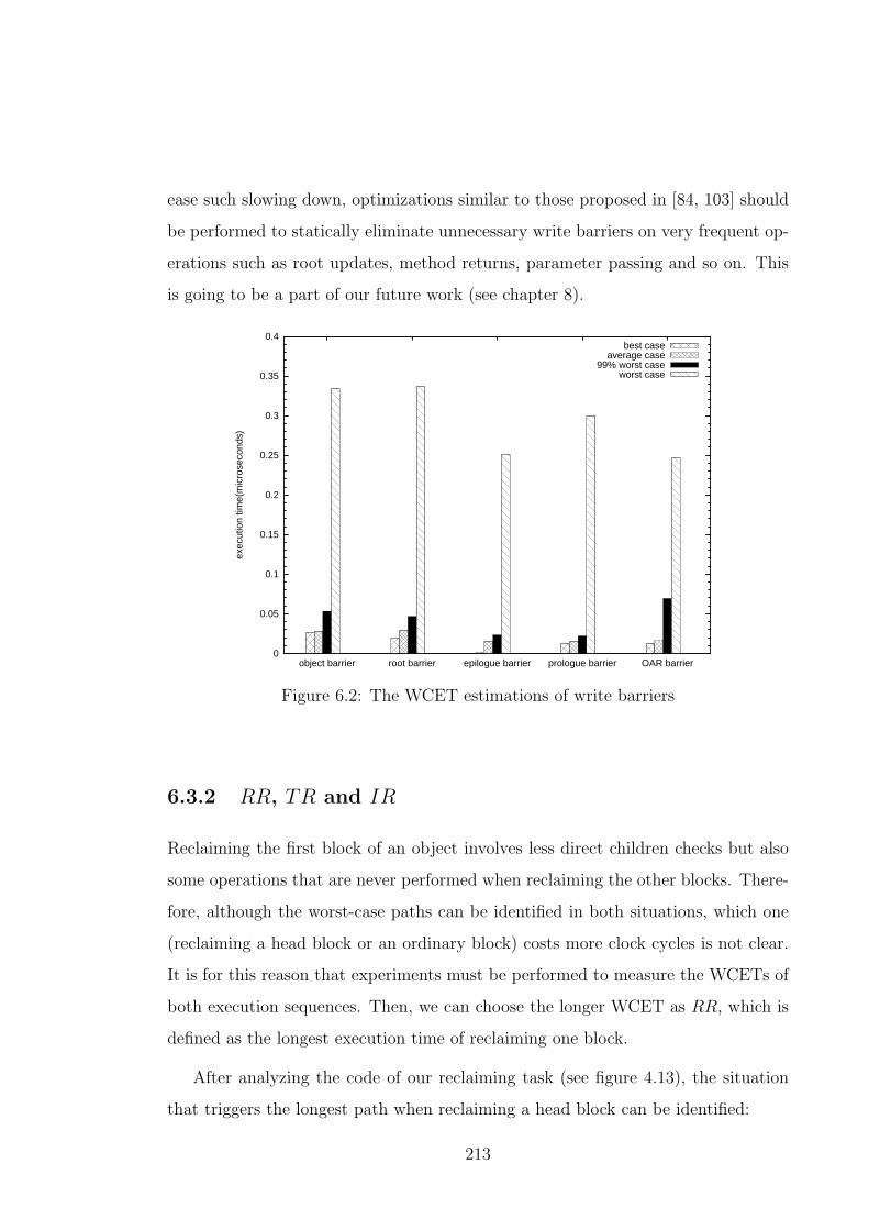
ease such slowing down, optimizations similar to those proposed in [84, 103] should

be performed to statically eliminate unnecessary write barriers on very frequent op-

erations such as root updates, method returns, parameter passing and so on. This

is going to be a part of our future work (see chapter 8).

0

0.05

0.1

0.15

0.2

0.25

0.3

0.35

0.4

OAR barrierprologue barrierepilogue barrierroot barrierobject barrier

exec

utio

n tim

e(m

icro

seco

nds)

best caseaverage case

99% worst caseworst case

Figure 6.2: The WCET estimations of write barriers

6.3.2 RR, TR and IR

Reclaiming the first block of an object involves less direct children checks but also

some operations that are never performed when reclaiming the other blocks. There-

fore, although the worst-case paths can be identified in both situations, which one

(reclaiming a head block or an ordinary block) costs more clock cycles is not clear.

It is for this reason that experiments must be performed to measure the WCETs of

both execution sequences. Then, we can choose the longer WCET as RR, which is

defined as the longest execution time of reclaiming one block.

After analyzing the code of our reclaiming task (see figure 4.13), the situation

that triggers the longest path when reclaiming a head block can be identified:

213

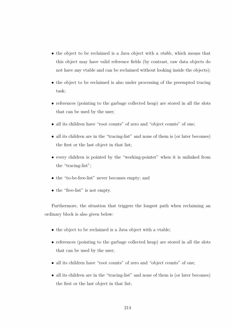
• the object to be reclaimed is a Java object with a vtable, which means that

this object may have valid reference fields (by contrast, raw data objects do

not have any vtable and can be reclaimed without looking inside the objects);

• the object to be reclaimed is also under processing of the preempted tracing

task;

• references (pointing to the garbage collected heap) are stored in all the slots

that can be used by the user;

• all its children have “root counts” of zero and “object counts” of one;

• all its children are in the “tracing-list” and none of them is (or later becomes)

the first or the last object in that list;

• every children is pointed by the “working-pointer” when it is unlinked from

the “tracing-list”;

• the “to-be-free-list” never becomes empty; and

• the “free-list” is not empty.

Furthermore, the situation that triggers the longest path when reclaiming an

ordinary block is also given below:

• the object to be reclaimed is a Java object with a vtable;


that can be used by the user;

• all its children have “root counts” of zero and “object counts” of one;

• all its children are in the “tracing-list” and none of them is (or later becomes)

the first or the last object in that list;

214

• every children is pointed by the “working-pointer” when it is unlinked from

the “tracing-list”;

• the “to-be-free-list” never becomes empty; and

• the “free-list” is not empty.

Then, experiments can be performed to get the execution times of both worst-

case paths. The results can be found in figure 6.3 where the execution times under

the name “Block1” are those of reclaiming a head block (through the worst-case

path) while those under the name “Block2” are the execution times of reclaiming

an ordinary block (through the worst-case path as well).

0

0.2

0.4

0.6

0.8

Block1Block2

exec

utio

n tim

e(m

icro

seco

nds)



Figure 6.3: The WCET estimations of block reclamation

As illustrated in figure 6.3, the execution times of reclaiming an ordinary block

are usually longer than those of reclaiming a head block. Particularly, the WCET of

reclaiming an ordinary block (0.785325 microseconds, or 1178 clock cycles) is longer

than the other one (0.727326 microseconds) so it is chosen to be the value of RR.

215

As defined in table 5.1, RR is the worst-case computation time needed to reclaim

a memory block. If any acyclic garbage exists at the free memory producer release

point, this is going to be exactly the free memory producer latency. Otherwise, the

free memory producer latency of our approach is going to be comparable with that

of a pure tracing collector. Shortly, we will compare the two different free memory

producer latencies.

Similarly, the longest execution time of tracing a head block may be different

from that of tracing an ordinary block. Therefore, experiments must be performed

to measure both WCETs as well. Intuitively, it is the longer WCET that is going

to be chosen as TR. However, the situations that trigger the longest paths when

tracing either a head or an ordinary block are identical:

• the object to be processed is a Java object with a vtable;

• the object to be processed has not been reclaimed;


that can be used by the user; and

• all its children are in the “white-list”.

Then, experiments can be performed to get the execution times of both worst-

case paths. The results can be found in figure 6.4 where the execution times under

the name “Block1” are those of tracing a head block (through the worst-case path)

while those under the name “Block2” are the execution times of tracing an ordinary

block (through the worst-case path as well).

As illustrated in figure 6.4, the WCET of tracing an ordinary block (0.775326

microseconds, or 1163 clock cycles) is higher than that of tracing a head block

(0.735326 microseconds) so it is chosen to be the value of TR. As can be seen in

figures 6.3 and 6.4, the longest time required to trace a block is even a little shorter

than the longest time required to reclaim a block. However, a tracing collector

216

0

0.2

0.4

0.6

0.8

Block1Block2

exec

utio

n tim

e(m

icro

seco

nds)



Figure 6.4: The WCET estimations of block tracing

can only identify garbage when, at least, all the live objects have been processed.

Therefore, the free memory producer latency of a tracing collector is actually m

times the length of TR where m is determined by either the maximum amount of

live memory or the heap size. On the other hand, the free memory producer latency

of the reference counting component (assuming that acyclic garbage exists) is fixed

at RR.

Moreover, the gaps between the WCETs and the 99% worst execution times in

figure 6.3 and 6.4 become (relatively) smaller than those in figure 6.2. To our best

knowledge, this is because each write barrier execution has fewer memory accesses

than either reclaiming or tracing a block, which suggests that write barriers have

fewer chances of encountering cache misses. Therefore, most tests on write barriers

have good cache performance, although a handful of tests do occasionally suffer

more cache misses. In the other two experiments, much fewer tests have as good

cache performance as the write barrier tests so the aforementioned gaps shrink.

Finally, the costs of traversing the “white-list” and initializing each object within

217

it can be obtained from experiments. First of all, the situation that triggers the

longest path when initializing an object is presented:

• the object under initialization has a “root-count” greater than zero; and

• the “tracing-list” is not empty.

The results are given in figure 6.5 (under the name “Root Objects”) and the

execution times of marking an object white (under the name “Other Objects”) is

also presented for comparison purposes only. The WCETs of both operations are

0.165998 microseconds (249 clock cycles) and 0.141999 microseconds respectively.

0

0.05

0.1

0.15

0.2

Other ObjectsRoot Objcets

exec

utio

n tim

e(m

icro

seco

nds)



Figure 6.5: The WCET estimations of tracing initialization

6.3.3 Worst-Case Blocking Time

In chapter 3, we argued that the user tasks should always be able to preempt the

real-time garbage collectors within a short, bounded time. The most crucial factor

that influences this feature is the longest execution path, in a garbage collector and

218

all the other related operations, that has to be performed atomically. In order to

perform the schedulability analysis proposed in chapter 5 and support the argument,

in chapter 4, that our garbage collector and related operations only introduce an

insignificant worst-case blocking time to any release of any task (including the GC

tasks), experiment results on the WCETs of the critical sections in our system are

to be presented in this subsection.

First of all, it should be made clear that the length of the worst-case blocking

time in a specific implementation of our system can be different from the others

(even if they are implemented on the same platform and in the same environment).

This is because they may be configured to protect several adjacent critical sections

as a whole so as to reduce the synchronization costs. However, this inevitably affects

the worst-case blocking time. In this subsection, the worst-case blocking time of our

current implementation will be presented and the corresponding synchronization

granularity will be discussed as well. By changing the synchronization granularity,

the worst-case blocking time and synchronization costs can be tuned to meet differ-

ent system requirements. As discussed in chapter 4, critical sections in our system

are mainly introduced by the GC tasks, write barriers and allocators.

In the reclaiming task, the critical sections introduced by the processing of the

“to-be-free-list” include the execution sequences that update the reference counts

of each direct child of the object being processed; move that child to the end of

the “to-be-free-list” when necessary; and link each free block to the end of the

“free-list”. However, protecting each of such critical sections individually is too ex-

pensive. Therefore, it is actually each individual block that is processed atomically.

Furthermore, the processing of the current snapshot of the “white-list-buffer” also

introduces critical sections in which each block can be safely linked to the end of the

“free-list”. However, since such critical sections are shorter, the worst-case blocking

time introduced by the reclaiming task is the WCET of reclaiming any block, which

is 0.785325 microseconds.

In the tracing task, the garbage collection initialization of each object should

219

be performed atomically, which either marks that object white or links it to the

“tracing-list”. The WCETs of such operations have been given in the previous

subsection (0.141999 and 0.165998 microseconds respectively). Moreover, the pro-

cessing of each child during the marking phase must be performed atomically as

well. Based on the aforementioned reason, this cannot be protected individually.

Therefore, our tracing task is implemented to protect each block (rather than each

reference field) during the marking phase. Consequently, the longest blocking time

introduced by the tracing component is 0.775326 microseconds (the value of TR).

As discussed in chapter 4, every outermost if branch in the write barrier pseu-

docode (see figure 4.8, 4.9, 4.10, 4.11, 4.12) must be executed atomically. However,

in order to reduce the synchronization and write barrier costs, each write barrier,

rather than a part of it, is executed atomically. Therefore, the WCETs of write

barriers given in subsection 6.3.1 can also be interpreted as the worst-case blocking

times introduced by write barriers, the highest value of which is 0.33733 microsec-

onds.

Also in chapter 4, we argued that, in our allocator, a certain number of blocks in

the “free-list” must be traversed and initialized atomically as a group so as to reduce

the synchronization costs. In this case, choosing the number of blocks that are to

be processed as a group has a significant impact on the worst-case blocking time

introduced by our garbage collector. Reducing the number of lock/unlock operations

should not come at cost of a significant increase in the worst-case blocking time.

Figure 6.6 illustrates a relation between the worst-case blocking time introduced

by the allocator and the number of blocks that are to be processed as a group.

Intuitively, the best results should be those close to and less than the longest blocking

time already known, which is the value of RR. As illustrated by figure 6.6, processing

eight blocks as a group gives a WCET of 0.71666 microseconds (1075 clock cycles),

which is the closest WCET to the worst-case blocking time known so far (0.785325

microseconds). Thus, it is decided to protect the allocator’s processing of every

8 blocks. As a result, the longest garbage collection related blocking time that

220

could be encountered in our system is only 0.785325 microseconds (the value of RR

and also B). Because of such a feature, the shortest hard real-time deadline we

can manage in the current implementation is 90 microseconds (600000 successful

releases). Indeed, our garbage collection algorithm has much less influence to this

value than the underlying platform. If the whole implementation can be ported

onto the “x86” architecture MaRTE OS, the results would be even better since

the synchronization overheads can be expected to be significantly lower and the

operating system can deliver more sophisticated real-time services.

0

0.1

0.2

0.3

0.4

0.5

0.6

0.7

0.8

0.9

1

1.1

1.2

1.3

0 2 4 6 8 10 12 14 16 18 20

The

leng

ths

of c

irtic

al s

ectio

ns in

the

allo

cato

r(m

icro

seco

nds)

The number of blocks to be allocated atomically



Figure 6.6: The relation between the worst-case blocking time introduced by the

allocator and the number of blocks that are to be processed as a group

6.3.4 Allocation

Based on the configuration choice made in the previous subsection, the execution

times of our allocator can be measured. Because our allocator has a complexity of

O(n) where n denotes the number of blocks requested, the execution times of our

allocator should be measured for different allocation requests. The experimental

221

results are given in figure 6.7.

0 0.1 0.2 0.3 0.4 0.5 0.6 0.7 0.8 0.9

1 1.1 1.2 1.3 1.4 1.5 1.6 1.7 1.8 1.9

2 2.1 2.2 2.3

0 32 64 96 128 160 192 224 256 288 320 352 384 416 448 480

allo

catio

n tim

e(m

icro

seco

nds)

object size(bytes)



Figure 6.7: The relation between the computation time of the allocator and the

requested memory size

Notice that data in figure 6.7 do not include the costs of Java language side

preparations for the calls to our allocator (for example, size estimation, class initial-

ization and so on). The costs of the corresponding object’s constructor are excluded

as well. As other results in this section, figure 6.7 does not include the synchroniza-

tion costs too. If m blocks are requested, the number of lock/unlock pairs in our

allocator will be⌈

m8

⌉

. As illustrated by figure 6.7, the execution times are usually

linear and proportional to the requested sizes, with only a few exceptions. This fig-

ure also demonstrates the importance of cache and pipelines on the execution times

not only by the differences between the WCET curve and the others, but also by the

fact that three out of four curves exhibit big jumps when the request size reaches

480 bytes, which leads to more cache (and perhaps also pipeline) misses.

222

Tasks Cj Tj(Dj) aj cggj maxLj

1 1 5 320 0 320

2 2 10 960 192 1600

3 5 50 1920 320 3200

4 12 120 5760 640 9600

Table 6.1: Hard real-time task set 1

Tasks Cj Tj(Dj) aj cggj maxLj

1 1 5 640 192 640

2 2 10 1920 576 3200

3 5 50 3840 1152 6400

4 12 120 11520 3456 19200

Table 6.2: Hard real-time task set 2

6.3.5 Synthetic Examples

With the above information, we can perform analyses of some synthetic hard real-

time task sets6. Notice that other similar task sets with task numbers up to 97 have

been analyzed and tested, which all give similar results. Due to the limitation on

space, we only present the results of the two task sets given in table 6.1 and 6.2.

All the values in tables hereafter are measured in milliseconds for time or bytes

for space. Priorities are assigned according to DMPO. Furthermore, a non-real-time

task which simply performs an infinite loop executes at a priority lower than all the

tasks in table 6.1 or 6.2. For simplicity and without loss of generality, only the GC

tasks are scheduled according to dual-priority algorithm. We will apply dual-priority

scheduling to other hard real-time tasks in our future work.

The execution time of a pair of operations that protect critical sections on our

6We were forced to use synthetic examples in our experiments because of the lack of serious

benchmark programs written in real-time Java. In fact, synthetic workloads are widely used by

the real-time community [105].7The number of tasks is limited by the number of timers in our platform.

223

platform is 2.4 microseconds according to our tests. As a result, we adjust the RR

to 3.19 microseconds, TR to 3.18 microseconds, IR to 2.57 microseconds and finally

B to 3.19 microseconds. To perform static analysis, the maximum amount of live

memory Lmax8 is calculated first according to [60]. The maximum amount of live

memory of all the hard real-time tasks in task set 1 and 2 are estimated as 14080

and 27520 bytes respectively and we set the maximum amount of static live memory

to be 9344 bytes for both task sets. Therefore, Lmax cannot exceed 23424 bytes for

task set 1 or 36864 bytes for task set 2.

A Static Analysis for Task Set 1

Assume that the size of the garbage collected heap is 37056 bytes, then the formu-

lae 5.29 on page 181, 5.30 on page 182 and 5.31 on page 182 can be used to determine

the priorities, periods and deadlines of the GC tasks, as well as the amount of mem-

ory reserved to synchronize the user tasks and the reclaiming task. First, it is

assumed that the GC tasks execute at priorities below all the user tasks. Therefore,

Rpre can be calculated:

Rpre =

⌈

Rpre

5

⌉

(1 + RR · 10) +

⌈

Rpre

10

⌉

(2 + RR · 30) +

⌈

Rpre

50

⌉

(5 + RR · 60)

+

⌈

Rpre

120

⌉

(12 + RR · 180) + B (6.1)

Thus, Rpre = 33.3749ms and Fpre can be estimated:

Fpre =

⌈

33.3749

5

⌉

· 320 +

⌈

33.3749

10

⌉

· 960 +

⌈

33.3749

50

⌉

· 1920

+

⌈

33.3749

120

⌉

· 5760 = 13760bytes (6.2)

Therefore, H−Lmax−Fpre = 37056−23424−13760 = −128bytes which suggests

that such a priority scheme cannot result in a schedulable system. Consequently, the

8 Lmax includes all the per-object and per-block overheads.

224

priorities of the GC tasks are moved to between the task 3 and 4, and the previous

procedure must be performed again:

Rpre =

⌈

Rpre

5

⌉

(1+RR ·10)+

⌈

Rpre

10

⌉

(2+RR ·30)+

⌈

Rpre

50

⌉

(5+RR ·60)+B (6.3)

The result of this formula is Rpre = 9.3541ms. Then, Fpre can be calculated:

Fpre =

⌈

9.3541

5

⌉

· 320 +

⌈

9.3541

10

⌉

· 960 +

⌈

9.3541

50

⌉

· 1920 = 3520bytes (6.4)

Therefore, H−Lmax−Fpre = 37056−23424−3520 = 10112bytes and the current

priority scheme could result in a schedulable system. According to formula 5.29 on

page 181, a safe deadline D can be estimated by:

(

⌈

D

5

⌉

+1) ·0+(

⌈

D

10

⌉

+1) ·192+(

⌈

D

50

⌉

+1) ·320+(

⌈

D

120

⌉

+1) ·640 ≤10112

2(6.5)

which gives D = 120ms and CGGmax = 5056bytes. As this deadline is between

those of the task 3 and 4, the current priorities specified for the GC tasks are a

solution.

Then, the maximum amount of memory that could be allocated within one GC

period, NEWmax, can be calculated:

NEWmax = (

⌈

D

5

⌉

+ 1) · 320 + (

⌈

D

10

⌉

+ 1) · 960 + (

⌈

D

50

⌉

+ 1) · 1920

+ (

⌈

D

120

⌉

+ 1) · 5760 = 39680bytes (6.6)

According to equation 5.33 on page 186, the WCET of the reclaiming task is

given:

Creclaiming = RR · NEWmax = 3955.6us (6.7)

225

On the other hand, the WCET of the tracing task can be estimated as:

Ctracing = TR · (Lmax + CGGmax) + IR · NOI = TR · (732 + 158)

+ IR ·(1158 − 110)

2= 4176.88us (6.8)

Therefore, Creclaiming + Ctracing = 8.14ms. Given such information, a standard

response time analysis can be performed for all the hard real-time tasks including

the GC tasks.

R1 = 1.00319ms (6.9)

which meets the deadline of task 1 (5ms);

R2 =

⌈

R2

5

⌉

· 1 + 2 + B (6.10)

and therefore R2 = 3.00319ms which meets the deadline of task 2 (10ms);

R3 =

⌈

R3

5

⌉

· 1 +

⌈

R3

10

⌉

· 2 + 5 + B (6.11)

and thus R3 = 9.00319ms which meets the deadline of task 3 (50ms).

Rtracing =

⌈

Rtracing

5

⌉

· 1 +

⌈

Rtracing

10

⌉

· 2 +

⌈

Rtracing

50

⌉

· 5 + 8.14 + B (6.12)

and therefore Rtracing = 24.14319ms which meets the deadline of the GC tasks

(120ms).

According to equation 5.39 on page 190, the longest possible initial promotion

delay of the GC tasks can be calculated:

Y ′

gc = D − Rtracing = 120 − 24.14319 = 95.85681ms (6.13)

226

As discussed in chapter 5, the GC promotion delay has an impact on the worst-

case response times of those hard real-time tasks running at lower priorities than

the GC tasks. Moreover, the GC tasks may be always promoted earlier than their

promotion time because the amount of free memory may always drop below Fpre

before the specified promotion time. Therefore, specifying a long promotion delay

does not necessarily result in a better system. Consequently, we present the worst-

case response times of the task 4 when different initial GC promotion delays are

chosen.

R4 =

⌈

R4

5

⌉

· 1 +

⌈

R4

10

⌉

· 2 +

⌈

R4

50

⌉

· 5 +

⌈

R4 + Ygc

120

⌉

· 8.14 + 12 + B (6.14)

When 0ms ≤ Ygc ≤ 75.85681ms, R4 = 44.14319ms which meets its dead-

line, 120ms. On the other hand, when 75.85681ms < Ygc ≤ 95.85681ms, R4 =

66.28319ms which meets the deadline as well. Therefore, this example is schedula-

ble when any GC promotion delay between 0ms and 95.85681ms is chosen.

A Static Analysis for Task Set 2

Given the heap size 91520 bytes, the same static analysis can be performed for the

task set 2 as well. First of all, it is assumed that the GC tasks execute at priorities

lower than all the hard real-time user tasks. Then, the corresponding Rpre and Fpre

can be calculated:

Rpre =

⌈

Rpre

5

⌉

(1 + RR · 20) +

⌈

Rpre

10

⌉

(2 + RR · 60) +

⌈

Rpre

50

⌉

(5 + RR · 120)

+

⌈

Rpre

120

⌉

(12 + RR · 360) + B (6.15)


227

Fpre =

⌈

34.7466

5

⌉

· 640 +

⌈

34.7466

10

⌉

· 1920 +

⌈

34.7466

50

⌉

· 3840

+

⌈

34.7466

120

⌉

· 11520 = 27520bytes (6.16)

Therefore, H−Lmax−Fpre

2= 91520−36864−27520

2= 13568bytes and the current priority

scheme could result in a schedulable system. According to formula 5.29 on page 181,

a safe deadline D can be estimated by:

(

⌈

D

5

⌉

+1)·192+(

⌈

D

10

⌉

+1)·576+(

⌈

D

50

⌉

+1)·1152+(

⌈

D

120

⌉

+1)·3456 ≤ 13568 (6.17)

Thus, D = 30ms which corresponds to priorities between the task 2 and 3.

Consequently, we change the GC priorities and perform the previous procedure

again.

Rpre =

⌈

Rpre

5

⌉

(1 + RR · 20) +

⌈

Rpre

10

⌉

(2 + RR · 60) + B (6.18)

Hence, Rpre = 3.2584ms and Fpre can be estimated:

Fpre =

⌈

3.2584

5

⌉

· 640 +

⌈

3.2584

10

⌉

· 1920 = 2560bytes (6.19)


2= 91520−36864−2560




(

⌈

D

5

⌉

+1)·192+(

⌈

D

10

⌉

+1)·576+(

⌈

D

50

⌉

+1)·1152+(

⌈

D

120

⌉

+1)·3456 ≤ 26048 (6.20)

Therefore, D = 120ms which corresponds to priorities between the task 3 and

4 (the priorities lower than the task 4 are already proven to be unsuitable for the

228

GC tasks). Consequently, we change the GC priorities and perform the previous

procedure again.

Rpre =

⌈

Rpre

5

⌉

(1+RR·20)+

⌈

Rpre

10

⌉

(2+RR·60)+

⌈

Rpre

50

⌉

(5+RR·120)+B (6.21)


Fpre =

⌈

9.705

5

⌉

· 640 +

⌈

9.705

10

⌉

· 1920 +

⌈

9.705

50

⌉

· 3840 = 7040bytes (6.22)


2= 91520−36864−7040




(

⌈

D

5

⌉

+1)·192+(

⌈

D

10

⌉

+1)·576+(

⌈

D

50

⌉

+1)·1152+(

⌈

D

120

⌉

+1)·3456 ≤ 23808 (6.23)

Hence, D = 120ms. As the new deadline corresponds to the same priorities

as previously assumed, the whole procedure completes. Moreover, CGGmax =

23808bytes.

Then, the maximum amount of memory that could be allocated within one GC

period, NEWmax, can be calculated:

NEWmax = (

⌈

D

5

⌉

+ 1) · 640 + (

⌈

D

10

⌉

+ 1) · 1920 + (

⌈

D

50

⌉

+ 1) · 3840

+ (

⌈

D

120

⌉

+ 1) · 11520 = 79360bytes (6.24)

According to equation 5.33 on page 186, the WCET of the reclaiming task is

given:

229


On the other hand, the WCET of the tracing task can be estimated as:


+ IR ·(2860 − 220)

2= 9421.68us (6.26)

Therefore, Creclaiming + Ctracing = 17.34ms. Given such information, a standard

response time analysis can be performed for all the hard real-time tasks including

the GC tasks.

R1 = 1.00319ms (6.27)


R2 =

⌈

R2

5

⌉

· 1 + 2 + B (6.28)


R3 =

⌈

R3

5

⌉

· 1 +

⌈

R3

10

⌉

· 2 + 5 + B (6.29)


Rtracing =

⌈

Rtracing

5

⌉

· 1 +

⌈

Rtracing

10

⌉

· 2 +

⌈

Rtracing

50

⌉

· 5 + 17.34 + B (6.30)

and therefore RGC = 38.34319ms which meets the deadline of the GC tasks (120ms).



Y ′

gc = D − Rtracing = 120 − 38.34319 = 81.65681ms (6.31)

230

Parameters task1 task2

H 37056(1.58Lmax) 91520(2.48Lmax)

Fpre 3520 7040

D 120 120

NEWmax 39680 79360

Ctracing 4.18 9.43

Creclaiming 3.96 7.92

Rtracing 24.14319 38.34319

GC utilization 6.78% 14.45%

Table 6.3: GC parameters

Based on the same reason discussed previously, we present the worst-case re-

sponse times of the task 4 when different initial GC promotion delays are chosen.

R4 =

⌈

R4

5

⌉

· 1 +

⌈

R4

10

⌉

· 2 +

⌈

R4

50

⌉

· 5 +

⌈

R4 + Ygc

120

⌉

· 17.34 + 12 + B (6.32)





All the results are summarized in table 6.39.

Given these parameters, we execute both task sets with our garbage collector

to justify the correctness of our algorithm and static analyses. Six different GC

promotion delays are selected for each task set to compare their impacts on the

memory usage of our system.

All the configurations of both task sets have been evaluated for 1000 hyperpe-

9GC utilization describes how much CPU time is dedicated to garbage collection. If a garbage

collector is scheduled periodically, GC utilization is the ratio between the WCET of the garbage

collector and its period.

231

riods10 (previous work reports feasibility only after 100 hyperperiods [60]) and no

deadline miss or user task blocking (by the garbage collector due to the lack of free

memory) has been reported. This is theoretically proven based on the informa-

tion about user tasks’ behaviour, heap size, RR, TR and IR rather than empirical

observations.

However, when the applications run longer, sporadic deadline misses appear and

the user tasks can be blocked occasionally due to the lack of free memory. This is

mainly because the underlying platform fails to provide hard real-time supports (for

example, the operating system may decide to execute some other tasks or operations

with even higher priorities than all of our user tasks). In order to prove this, all the

allocations and reference assignments in the user tasks are eliminated. Instead, more

floating operations are added. The garbage collector is also switched off so that the

proposed garbage collection algorithm and other relevant ones have no influence at

all to the user tasks and their scheduling. When such a task set executes, sporadic

deadline misses can still be observed. In order to prove that the occasional user task

blockings (caused by garbage collector) are not caused by memory leak accumulation

that can only be observed after a very long time, the amount of free memory at the

beginning of every GC cycle is recorded and a stable amount of free memory is

always provided.

The memory usage of task set 1 is presented in figure 6.8, 6.9, 6.10, 6.11, 6.12

and 6.1311.

On the other hand, the memory usage of task set 2 is presented in figure 6.14,

6.15, 6.16, 6.17, 6.18 and 6.19 respectively.

These figures illustrate the fundamental difference between our approach and

a pure tracing one, which is that the amount of free memory in our system no

longer decreases monotonically in each GC period. This is because our approach

10 Hyperperiod defines the minimum length of time sufficient to create an infinitely repeatable

schedule.11 Allocation id x means the xth allocation.

232

0

100

200

300

400

500

600

700

800

900

1000

1100

0 400 800 1200 1600 2000 2400

free

mem

ory(

bloc

ks)

allocation id

Lmax

Fpre

free memory

Figure 6.8: Task set 1 with promotion delay 0ms

0

100

200

300

400

500

600

700

800

900

1000

1100

0 400 800 1200 1600 2000 2400

free

mem

ory(

bloc

ks)

allocation id

Lmax

Fpre

free memory


233

0

100

200

300

400

500

600

700

800

900

1000

1100

0 400 800 1200 1600 2000 2400

free

mem

ory(

bloc

ks)

allocation id

Lmax

Fpre

free memory


0

100

200

300

400

500

600

700

800

900

1000

1100

0 400 800 1200 1600 2000 2400

free

mem

ory(

bloc

ks)

allocation id

Lmax

Fpre

free memory


234

0

100

200

300

400

500

600

700

800

900

1000

1100

0 400 800 1200 1600 2000 2400

free

mem

ory(

bloc

ks)

allocation id

Lmax

Fpre

free memory


0

100

200

300

400

500

600

700

800

900

1000

1100

0 400 800 1200 1600 2000 2400

free

mem

ory(

bloc

ks)

allocation id

Lmax

Fpre

free memory


235

0

200

400

600

800

1000

1200

1400

1600

1800

2000

2200

2400

2600

2800

0 800 1600 2400 3200 4000 4800

free

mem

ory(

bloc

ks)

allocation id

Lmax

Fpre

free memory


0

200

400

600

800

1000

1200

1400

1600

1800

2000

2200

2400

2600

2800

0 800 1600 2400 3200 4000 4800

free

mem

ory(

bloc

ks)

allocation id

Lmax

Fpre

free memory


236

0

200

400

600

800

1000

1200

1400

1600

1800

2000

2200

2400

2600

2800

0 800 1600 2400 3200 4000 4800

free

mem

ory(

bloc

ks)

allocation id

Lmax

Fpre

free memory


0

200

400

600

800

1000

1200

1400

1600

1800

2000

2200

2400

2600

2800

0 800 1600 2400 3200 4000 4800

free

mem

ory(

bloc

ks)

allocation id

Lmax

Fpre

free memory


237

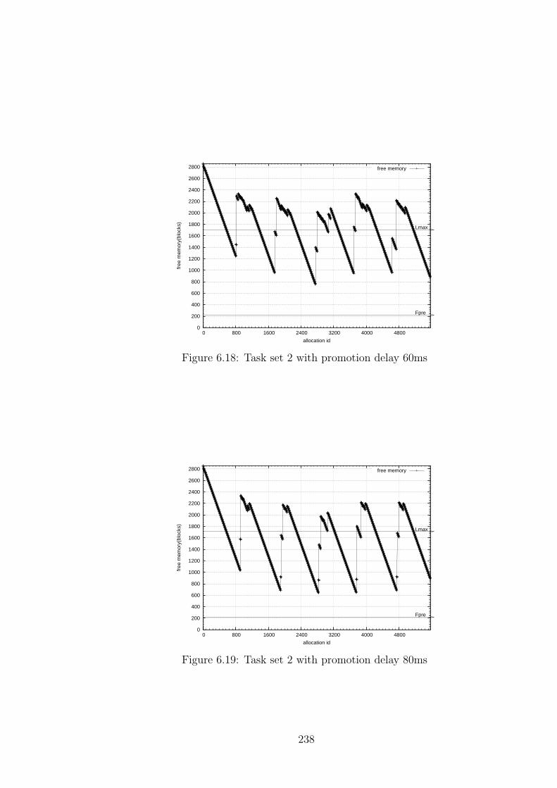
0

200

400

600

800

1000

1200

1400

1600

1800

2000

2200

2400

2600

2800

0 800 1600 2400 3200 4000 4800

free

mem

ory(

bloc

ks)

allocation id

Lmax

Fpre

free memory


0

200

400

600

800

1000

1200

1400

1600

1800

2000

2200

2400

2600

2800

0 800 1600 2400 3200 4000 4800

free

mem

ory(

bloc

ks)

allocation id

Lmax

Fpre

free memory


238

possesses a relatively lower free memory producer latency. Not only tracing but also

reclamation can be performed incrementally. Secondly, the later the promotion time

is, the smaller the space margin we will have, which suggests that users tasks are

given preference over GC tasks by squeezing the heap harder.

Finally, we choose [87] as an example of pure tracing collectors with which we

compare our algorithm. According to their analysis, our task set 1 along with a pure

tracing GC task is infeasible since (∀D)(∑

j∈task1

(⌈

DTj

⌉

· aj

)

> (H − Lmax)/2) but

for task set 2, we can expect the longest deadline to be 30 milliseconds which implies

a 31.44% GC utilization12 (ours is 14.45%). Notice that the user task utilization of a

pure tracing system can be lower than ours due to the fact that our write barriers are

more expensive than their pure tracing counterparts. However, this cannot change

the garbage collection work amount because user tasks are periodically scheduled.

On the other hand, if we assume the priority and utilization of the pure tracing

GC task are the same as those of our GC tasks, the pure tracing period will be

61.66 milliseconds for task set 1 or 65.26 milliseconds for task set 2. According to

the static analysis in [87], this corresponds to a heap of 64384 bytes (2.75Lmax) for

task set 1 or 120064 bytes (3.26Lmax) for task set 2. By contrast, our heap sizes are

theoretically proven as 1.58Lmax or 2.48Lmax. Since the heap sizes and Lmax for both

approaches are presented with the same per-object and per-block space overheads,

the ratios between the heap sizes and the Lmax can be compared between the two

approaches.

Notice that the pure tracing static analysis used to compare our approach with

a pure tracing one does not take the extra releases of user tasks discussed in chapter

5 into consideration. Therefore, their theoretical bounds of heap sizes and GC

utilizations are actually underestimated. After the pure tracing static analysis is

corrected, both task sets become infeasible when they are executed along with a

pure tracing collector (given that the heaps used have the same size as ours). On

the other hand, if we assume the priority and utilization of the pure tracing GC

12 We assume that the pure tracing GC task has the same WCET as that of our tracing task.

239

task are the same as those of our GC tasks, the pure tracing period will be 61.66

milliseconds for task set 1 or 65.26 milliseconds for task set 2. Consequently, the

heap sizes will be 82304 bytes (3.52Lmax) for task set 1 or 155904 bytes (4.23Lmax)

for task set 2. By contrast, our heap sizes are theoretically proven as 1.58Lmax or

2.48Lmax.

6.3.6 The Response Time of A Non-Real-Time Task

In order to explore the performance of a non-real-time task13 under dual priority

scheduling scheme, we modify the non-real-time task in task set 1 so that it starts

at the same time as all the other tasks and performs certain number of iterations of

floating computation. On the one hand, it is configured to execute three different

numbers of iterations of floating computation, denoted as iteration A, B and C

respectively. On the other hand, four different GC promotion delays are used to test

the corresponding non-real-time task response times, which are illustrated in figures

6.20, 6.21 and 6.22. For each configuration (with a specific number of iterations and

a specific GC promotion delay), eight executions were performed and the results

are presented in terms of the best value, the worst value and the average value. As

can be seen, dual priority scheduling provides 4.34 - 5.78 milliseconds improvements

on “iteration A” executions’ average response times compared with fixed priority

scheduling. It also provides 1.16 - 8.62 milliseconds improvements on “iteration B”

executions’ average response times compared with fixed priority scheduling. Finally,

it gives −0.04 - 0.77 milliseconds improvements on “iteration C” executions’ average

response times compared with fixed priority scheduling.

The reason why “iteration C” executions’ average response times cannot be

improved as much as the other configurations is that the non-real-time task with

this number of iterations always has a response time Rsoft where Rsoft mod 120 >

13 Recall that a non-real-time task does not allocate any memory in our system. Neither does it

make any cyclic garbage in the heap.

240

18

19

20

21

22

23

24

25

26

27

28

29

30

31

32

33

34

35

promotion 90promotion 50promotion 10promotion 0

resp

onse

tim

e(m

illis

econ

ds)

best caseworst case

average case

Figure 6.20: Response time of a non-real-time task (iteration A) with different GC

promotion delays

34

35

36

37

38

39

40

41

42

43

44

45

46

47

48

49

50

51

52


resp

onse

tim

e(m

illis

econ

ds)

best caseworst case

average case

Figure 6.21: Response time of a non-real-time task (iteration B) with different GC

promotion delays

90milliseconds, assuming that the GC tasks never interfere the non-real-time task

during the GC period where it finishes. Therefore, even delaying the GC tasks for

90 milliseconds cannot influence the response time significantly. Indeed, this is a

characteristic of all the dual-priority scheduled systems rather than a specific issue

241

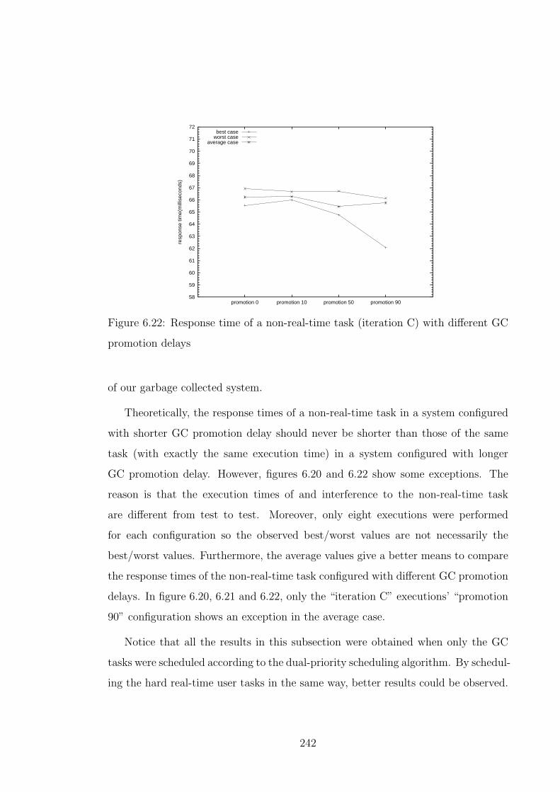
58

59

60

61

62

63

64

65

66

67

68

69

70

71

72


resp

onse

tim

e(m

illis

econ

ds)

best caseworst case

average case

Figure 6.22: Response time of a non-real-time task (iteration C) with different GC

promotion delays

of our garbage collected system.

Theoretically, the response times of a non-real-time task in a system configured

with shorter GC promotion delay should never be shorter than those of the same

task (with exactly the same execution time) in a system configured with longer

GC promotion delay. However, figures 6.20 and 6.22 show some exceptions. The

reason is that the execution times of and interference to the non-real-time task

are different from test to test. Moreover, only eight executions were performed

for each configuration so the observed best/worst values are not necessarily the

best/worst values. Furthermore, the average values give a better means to compare

the response times of the non-real-time task configured with different GC promotion

delays. In figure 6.20, 6.21 and 6.22, only the “iteration C” executions’ “promotion

90” configuration shows an exception in the average case.

Notice that all the results in this subsection were obtained when only the GC

tasks were scheduled according to the dual-priority scheduling algorithm. By schedul-

ing the hard real-time user tasks in the same way, better results could be observed.

242

6.4 Summary

In this chapter, the prototype implementation of our algorithm has been intro-

duced. More specifically, the architecture, memory organization and limitations of

our current implementation were discussed. Because our system is implemented

on a standard operating system, the predictability and performance of the real-time

applications could be undermined by any non-real-time activity in the operating sys-

tem and non-real-time applications. Moreover, because the real-time applications

on our implementation can only be performed in user mode, expensive lock/unlock

operations, rather than the cheap interrupt switch on/off, have to be used to protect

critical sections. All such issues have impacts on the maximum blocking time, over-

all overheads, maximum task number, context switch costs, timer accuracy and so

on. Therefore, porting the current implementation to a better platform is desired.

Many experiments were presented in this chapter as well. At first, the costs of

write barrier were studied. Then, the execution times required to reclaim and trace

each memory block as well as the costs of initializing each object by the tracing task

were also explored. This was followed by the efforts of identifying the worst-case

blocking time of the whole system, i.e. the longest critical section in our garbage

collector, write barriers and allocator. A choice was also made on the number of

blocks that should be allocated atomically so that the least number of lock/unlock

operations is required and the length of the longest critical section is not changed.

Moreover, the execution times of our allocator were also presented.

Two synthetic examples were analyzed and tested to prove the correctness of our

analysis, algorithm and implementation. Free memory changes of both examples

were presented and compared. We also explained the uniqueness of our approach

by investigating the free memory change figures. Finally, a non-real-time task’s

response times were tested to demonstrate how the dual-priority scheduling algo-

rithm improves the performance of a non-real-time task and when the dual-priority

scheduling algorithm cannot improve them.

243

Chapter 7

Relaxing the Restrictions on Soft-

and Non-Real-Time Tasks

By using bandwidth preserving algorithms such as [63, 36], the execution of the soft-

and non-real-time tasks consumes at most a predetermined processor bandwidth so

that the remaining processor capacity is still high enough for the hard real-time tasks

to meet their deadlines. However, the aforementioned research work does not take

the memory consumption of the soft- and non-real-time tasks into consideration,

which could cause the hard real-time tasks to run out of memory. In order to avoid

such an issue in our system, we initially assumed that the user tasks other than the

hard real-time ones neither produce any cyclic garbage nor allocate memory from

the heap (see chapter 4 and 5). Although this helps result in hard real-time task sets

that never run out of memory, it is a far too rigid restriction for the soft- and non-

real-time tasks. In this chapter, a multi-heap approach will be presented to bound

the memory impacts from the soft- and non-real-time tasks to the hard real-time

ones while still allowing the soft- and non-real-time tasks’ flexible use of memory.

The proposed algorithm and scheduling property will be introduced first. Then, the

static analysis discussed in chapter 5 will be updated to model the temporal and

spatial behaviours of the new system. Moreover, we will also introduce how to use

244

an automatic tool to enforce our reference assignment rules statically. Finally, a

synthetic example will be presented and evaluated.

7.1 Algorithm and Scheduling

In chapters 2 and 3, a few state-of-the-art real-time garbage collectors were discussed.

Among them, Metronome along with Siebert, Ritzau and Kim et al.’s algorithms

do not distinguish hard real-time and soft/non-real-time tasks. Neither do they

distinguish hard real-time and soft/non-real-time allocations. Identical information

has to be derived from all the user tasks, irrespective of whether a task is hard

real-time or not. Otherwise, it would not be possible to perform the proposed

static analyses. However, the information required by the proposed static analyses,

which are used to provide hard real-time guarantees, is usually hard and expensive

to obtain. Therefore, a real-time garbage collector designer should always assume

that very limited information about soft/non-real-time tasks is available. Thus, the

aforementioned garbage collectors cannot easily work well with soft- or non-real-time

user tasks.

In Henriksson’s algorithm, a GC task runs at a priority between hard real-time

and soft/non-real-time user tasks to work on behalf of only the hard real-time user

tasks. On the other hand, each allocation of the soft/non-real-time task is preceded

by a certain amount of garbage collection work. Although memory requests and

garbage collection are treated differently in hard real-time and soft/non-real-time

tasks, identical information is still required for all the user tasks. Otherwise, no

guarantee could be given to the hard real-time tasks. Moreover, if a soft- or non-

real-time task allocates huge amount of memory, not only the soft- or non-real-time

tasks have to be slowed down (because more garbage collection work has to be

performed for each allocation), but also the GC task has to execute for a much

longer time, which could result in an infeasible system (or, increase the overall size

of memory). Finally, if any estimation of the soft- or non-real-time task’s memory

245

usage goes wrong, the whole system including the hard real-time part may fail.

Robertz and Henriksson’s algorithm does not explicitly deal with soft- or non-

real-time user tasks. However, they distinguish critical and non-critical memory

requests. A certain amount of memory is reserved for all the non-critical allocations.

If the budget is exhausted, the corresponding memory requests will be denied. By

requesting all the soft- or non-real-time tasks to issue non-critical allocations, their

impacts on the garbage collector, overall memory usage and eventually the execution

of the hard real-time tasks can be easily modeled without much knowledge about

the soft- or non-real-time tasks. However, if the soft- or non-real-time tasks are

given a huge budget (because they allocate huge amount of memory), the WCET

of the GC task will be dramatically increased, which could result in an infeasible

system. This is because the garbage collector has to process the whole heap.

Usually, the hard real-time tasks in a flexible real-time system only need a rela-

tively small processor bandwidth to meet their timing constraints while the soft- and

non-real-time tasks rely on a larger bandwidth to achieve adequate performance. It

is very likely that the memory usage of the two subsets has a similar feature as their

processor time distributions. That is, the soft- and non-real-time tasks could prob-

ably use more memory than the hard real-time ones. Therefore, running a unified

garbage collector in a unified heap for both task subsets can significantly influence

the schedulability of the hard real-time tasks. Moreover, it is not practical to ana-

lyze all the user tasks for the information required to run such a unified collector.

For example, ai and cggi can be hard to achieve for some tasks. Indeed, some in-

formation, such as period, is impossible to obtain for some tasks. Consequently, it

was decided to separate the heap into two which are used by the two task subsets

respectively (each heap should be larger than the maximum amount of live memory

of the corresponding task subset) and two collectors should be executed for different

heaps as well. Moreover, because how to achieve such separations is closely related

to the language under investigation, all the discussions made in this chapter are in

the context of the Java language.

246

On the one hand, the memory usage of the soft- and non-real-time tasks should

influence the hard real-time heap and the hard real-time garbage collector as little as

possible so that all the already proposed analyses can still be used without significant

modifications. On the other hand, although usually weaker than those provided for

the hard real-time tasks, assurances must be given to the allocation requests issued

by the soft- and non-real-time tasks as well.

By dividing the heap into two, the hard real-time tasks (RTSJ RealtimeThread1)

allocate memory only from the hard real-time heap whilst the soft- and non-real-time

tasks (standard Java Thread) allocate memory only from the soft- or non-real-time

heap (which heap to use is determined by the allocator automatically). However,

any user task could access an object/array in the heap other than the one in which

it is executing. This can be done by two means: 1) it could access an object/array

in the other heap by accessing a root variable; 2) it could access an object/array in

the other heap by accessing an object/array reference field stored in its own heap.

As will be discussed shortly, identical copies of the garbage collector data structures

and the same write barrier algorithm have been used for all the tasks so that soft-

or non-real-time objects referenced by roots (irrespective of which task owns the

root) can be identified in the same way as the hard real-time objects. Notice, they

are maintained in different “tracing-lists” or “white-lists”. Therefore, from both

collectors’ points of view, there is no difficulty in quickly finding all the objects

referenced by roots. However, if an object in heap A is referenced by an object in

heap B, the collector that processes heap A will have to consider such a reference as

a root for heap A or wait until the collector that processes heap B completes so that

all the objects in heap A that is referenced by heap B have been identified. In order

to completely avoid root scanning, we follow the latter approach to cope with the

1 In standard RTSJ, hard real-time user tasks are usually NoHeapRealtimeThread(s), which

never access the heap. Instead, they use scope and immortal memory to dynamically allocate

memory. In our system, the heap managed by a real-time garbage collector rather than the

scope/immortal memory is used by all the user tasks. Therefore, there is no reason to use No-

HeapRealtimeThread(s). Instead, we use RealtimeThread to represent hard real-time user tasks.

247

references between objects in two different heaps. Intuitively, it is not acceptable

to ask the hard real-time collector to wait for the completion of the soft- or non-

real-time collector so references from soft- or non-real-time objects to hard real-time

objects are forbidden in our system. Since the soft- or non-real-time tasks can still

access objects in the hard real-time heap through root variables, this restriction does

not dramatically influence the functionality of the application being developed.

In order to make sure that the amount of cyclic garbage in the hard real-time

heap never exceeds CGGmax during a hard real-time GC period, it is required that

the soft- or non-real-time tasks should never produce any cyclic garbage in the hard

real-time heap. However, they are free to produce any amount of cyclic garbage in

the soft- or non-real-time heap. Since the soft- and non-real-time tasks can neither

allocate any memory from the hard real-time heap nor produce any cyclic garbage

within that heap, all the discussions made in previous chapters still hold.

In the Java language, an object representing each thread (i.e. task) must be

created (by another thread) before that thread can be launched. Irrespective of

the type of the thread that is being created, a hard real-time thread creates any

thread object in the hard real-time heap while a standard Java thread creates thread

objects in the soft- or non-real-time heap. Therefore, it is possible that a (non-real-

time) standard Java thread object is allocated in the hard real-time heap and/or a

(hard real-time) RTSJ RealtimeThread object is allocated in the soft- or non-real-

time heap. Because such thread objects should obey the above inter-heap reference

rules as well, a (hard real-time) RTSJ RealtimeThread object may be unable to

reference hard real-time objects. Moreover, a (non-real-time) standard Java thread

object may be able to reference hard real-time objects. Figure 7.1 summaries all the

combinations.

As a thread object should always be able to reference objects allocated by its cor-

responding thread, allocating a RTSJ RealtimeThread object in the soft- or non-real-

time heap should be prohibited. Consequently, the Java “main” thread is treated as

a hard real-time thread in our system so that all the objects allocated by the “main”

248

Soft/Non-Real-TimeProgram Stack

Hard Real-TimeProgram Stack

Static Data Area

hard

soft

Hard Real-Time Heap

��

� �

��

� �Soft/Non-Real-Time Heap��

� � � �

��

hard

soft

hard

soft

RTSJ RealtimeThreadObjects

Standard Java ThreadObjects

Objects

Figure 7.1: The reference rules of our multi-heap approach

thread are in the hard real-time heap. Notice, a standard Java thread object cre-

ated by the “main” thread can reference any other hard real-time objects but the

objects created by that thread will be unable to reference any hard real-time object

including the thread object itself. As discussed in the previous chapter, (in our cur-

rent implementation) the system data structures created during the bootstrap of the

runtime system are stored in another heap which is not subject to garbage collection

so any reference to those data structures are legal (but which are never followed by

our (soft) GC tasks and write barriers). Any reference from the bootstrap heap to

the others is considered as a root variable.

The above rules have an implication that a standard Java program may be

unable to execute in our system. It is very common for a standard Java “main”

method to allocate some objects/arrays and then release a standard Java thread

which accesses the objects/arrays allocated in the “main” method through some

objects/arrays allocated by itself. In our system, all the objects/arrays allocated in

the “main” method are in the hard real-time heap. Therefore, the objects/arrays

249

allocated by a standard Java thread (which are in the soft- or non-real-time heap)

cannot reference them. One way to solve this problem is to modify every standard

Java program so that a new “main” method builds and launches a new standard

Java thread which executes the original “main” method. By doing so, the original

“main” method allocates objects/arrays in the soft- or non-real-time heap.

The soft- or non-real-time collector uses a set of data structures that are identical

to the hard real-time ones. In order to distinguish them, a prefix “soft-” should be

added to the name of every hard real-time data structure to represent its soft- or

non-real-time counterpart. For example, the soft- or non-real-time counterpart of

“tracing-list” is called “soft-tracing-list”. The tracing and reclaiming tasks also

have their soft- or non-real-time counterparts, i.e. the soft tracing task and the soft

reclaiming task.

As with the tracing task, the soft tracing task runs as a backup collector to

identify cyclic garbage objects. In order to guarantee that such garbage objects can

be found periodically and soft- or non-real-time objects referenced by the hard real-

time ones can always be identified alive, it is decided to integrate the soft tracing

task into the hard real-time task set and our dual-priority scheduling scheme. More

specifically, the execution of the soft tracing task must be modeled as a periodic hard

real-time task that executes a fixed length increment during each period. Moreover,

the hard real-time GC period D is used as the period and deadline of the soft

tracing task which runs at the priority lower than the GC tasks in either priority

bands (see figure 7.2). When the GC tasks are promoted due to any reason, the

soft tracing task should be promoted as well. When a new period comes, the soft

tracing task along with the GC tasks are released at lower band priorities. Further,

the interference from the soft tracing task to the low priority hard real-time tasks

can still be controlled because the soft tracing task suspends itself whenever enough

work has been done irrespective of which priority band it executes in.

By contrast, the soft reclaiming task should be as responsive as the soft- and

non-real-time tasks. Otherwise, the soft- and non-real-time tasks would have to wait

250

a long time when they have no free memory to use. Therefore, the soft reclaiming

task is designed to execute within the middle priority band, along with the soft- and

non-real-time user tasks. More precisely, the soft reclaiming task usually executes at

the lowest priority within the middle priority band. When a soft- or non-real-time

user task is blocked due to the lack of free memory, the soft reclaiming task inherits

its priority and reclaims enough free memory. Then, it goes back to the original

priority. If, however, the reclaiming task is preempted by another soft- or non-real-

time user task which then requests dynamic memory as well, the soft reclaiming

task should inherits the priority of that task and goes back to its original priority

when enough free memory has been reclaimed for both requests.

Because the soft reclaiming task is never suspended except when there is no

garbage to reclaim, it can execute when there is no soft- or non-real-time user

task executing (assuming no hard real-time task is promoted at that time). This

reduces the number of the aforementioned blockings. However, we cannot provide

any guarantee to such an improvement since it depends on when the soft- and non-

real-time tasks arrive, which is usually unknown. Another way to reduce the number

of the aforementioned blockings is to promote the reclaiming task to the upper

priority band along with the GC tasks and the soft tracing task. More specifically,

the soft reclaiming task has a budget in the upper priority band and it should

never use more than that budget within every period of that budget. The budget

is replenished periodically with the period equal to the hard real-time GC period

D. The soft reclaiming task executes at the priority between the tracing task and

the soft tracing task (see figure 7.2). When the GC tasks are promoted due to

any reason, both soft GC tasks should be promoted as well. When the budget

capacity is exhausted or a new period comes, the soft reclaiming task goes back to

its middle band priority. Therefore, on the one hand, a certain amount of progress

can be guaranteed for the soft reclaiming task during each D; on the other hand, the

interference from the soft reclaiming task to the hard real-time tasks is still bounded.

Notice that the execution of the soft reclaiming task before a GC promotion time

251

does not lead to the delay of the GC promotion time as the executions of the GC

tasks and the soft tracing task do.

Upper Band

Lower Band

Middle Band

Hard Real-Time User Tasks (promoted)

Hard Real-Time User Tasks (promoted)

The Reclaiming Task (promoted)

The Tracing Task (promoted)

The Soft Reclaiming Task (promoted)

The Soft Tracing Task (promoted)

Soft/Non-Real-Time User Tasks

The Soft Reclaiming Task (original)

The Reclaiming Task (original)

Hard Real-Time User Tasks(original)

The Tracing Task (original)

The Reclaiming Task (extra work)

Hard Real-Time User Tasks(original)

The Soft Tracing Task (original)

LowerPriority

HigherPriority

Figure 7.2: The new priority map of the system

The number of blocks (in the soft- or non-real-time heap) that have been re-

claimed is again used as the GC work metric for the soft reclaiming task. On the

other hand, the real execution time has to be used to measure the work amount of

the soft tracing task. The “work-amount” limits (budgets) must be large enough to

avoid starving the soft- or non-real-time tasks for too long but they should also be

small enough to allow a schedulable hard real-time task set and enough progress of

the soft- and non-real-time tasks. Notice, we cannot ensure that the soft- or non-

real-time tasks always get enough free memory when they are requesting. However, a

252

stable number of soft- or non-real-time blocks are guaranteed to be reclaimed within

each GC period given that enough garbage can always be recognised. Hence, a sta-

ble reclamation rate can be achieved for the soft- or non-real-time heap if enough

garbage can be identified. Moreover, because the soft tracing task neither initializes

objects allocated during initialization nor processes objects allocated during mark-

ing, the execution time of the soft tracing task is also bounded. Therefore, each

release of the soft tracing task can be finished within a bounded number of GC

periods. Consequently, soft- or non-real-time cyclic garbage can be found within a

bounded time interval. The maximum length of such an interval mainly depends

on the soft- or non-real-time heap size and the soft tracing task’s budget, both of

which should be specified by the designer of a given application.

The write barriers are modified in a way that an additional check is made for each

reference (passed to the write barrier) to see in which heap the referenced object

resides (as illustrated in figure 4.7, the “S” field of each object header provides

such information) and then different code can be used for objects in different heaps.

Notice that the same algorithm is used for objects in either heap and the only

difference is the data structures that are going to be accessed.

The reclaiming task is also modified. The only difference is that the new version

requires to check in which heap a child of the block being processed resides when

that child is found dead. Then, the dead child will be linked to the rear of the

“to-be-free-list” or the “soft-to-be-free-list” depending on in which heap the dead

child resides. Moreover, the only change made to the tracing task is that when an

object is going to be marked grey, a check must be made and the object should be

linked to the end of either “tracing-list” or “soft-tracing-list”. Intuitively, the above

extra checkings will increase the WCETs of both the reclaiming task and the tracing

task. However, moving the soft- or non-real-time objects will not increase the costs

because such costs are identical to those of moving hard real-time objects and they

have already been included into the previous WCET analyses.

The soft reclaiming task implements the algorithm as illustrated in figure 4.13.

253

However, it processes the “soft-to-be-free-list” along with the “soft-white-list-buffer”

and returns recycled memory to the “soft-free-list” instead. All the objects that

could be encountered by the soft reclaiming task are in the soft- or non-real-time

heap since there should be no reference from the soft- or non-real-time heap to the

hard real-time heap.

When it comes to the soft tracing task, the algorithm illustrated in figure 4.14

cannot be used directly. References from the hard real-time heap to the soft- or

non-real-time heap must be considered. As discussed previously, the soft tracing

task can only be executed when the tracing task is suspended, which means that

all the soft- or non-real-time objects referenced by hard real-time objects should

be already marked grey whenever the soft tracing task executes (given that the

initialization phase of the soft tracing task is atomic). However, after every time

the soft tracing task marks all the objects in the “soft-white-list” white, the object

liveness information provided by the previous release of the tracing task could be lost

(we have no way to determine which grey objects are referenced by hard real-time

objects and therefore should be kept grey during the soft tracing task initialization).

If the marking phase cannot be completed before the next release of the tracing task,

such lost information can be rebuilt and therefore no live object can be identified

as garbage by the soft tracing task. Although very unlikely, it is possible that the

soft tracing task finishes before the next release of the tracing task and therefore,

the aforementioned lost information cannot be rebuilt. Consequently, the algorithm

illustrated in figure 4.14 could cause live objects to be reclaimed by mistake.

In order to solve this problem, the order in which the initialization phase and the

marking phase should be performed is changed. The algorithm of the soft tracing

task is illustrated in figure 7.3. As can be seen, the marking operations, instead of

the initialization operations, are performed first. Therefore, the first release of the

soft tracing task cannot identify any garbage at all since there is no white object

at the beginning of its first marking phase. Indeed, every release of the soft tracing

task initializes objects white for the next release so the basic function of the soft

254

tracing task is still complete. By doing so, any lost liveness information is guaranteed

to be reconstructed before the next marking phase of the soft tracing task. More

specifically, because the liveness information can only be lost when initialization is in

progress, if such operations cannot be finished before the next release of the tracing

task, the lost information will be rebuilt before the initialization operations resume.

If, on the other hand, the initialization finishes before the next release of the tracing

task, the soft tracing task will be suspended until the release of the tracing task.

Then, the tracing task can rebuild the information required. Notice, the tracing

task and the write barriers could be confused by objects’ temporary colours during

any initialization phase of the soft tracing task. This is not going to be a problem

because: 1) there is not any black object in the soft- or non-real-time heap (the

temporarily black object would be marked white or grey before the next marking

phase of the soft tracing task); 2) any inter-heap reference that is missed during this

initialization phase can be identified by at latest the first release of the tracing task

after this initialization phase, which is definitely before the next marking phase of

the soft tracing task. Hence, there is not any live object that can be identified as

garbage by mistake in this new algorithm.

Indeed, what garbage collection algorithm to use for the soft- or non-real-time

heap has little to do with the behaviour of the hard real-time components, if only a

correct and efficient share of information can be achieved between the collectors and

the critical sections of the soft- or non-real-time collectors are not significantly longer

than their hard real-time counterparts. For example, different write barriers may be

implemented in different user tasks; incremental or generational tracing garbage col-

lection algorithms may be used alone for the soft- or non-real-time heap. Moreover,

if a soft- or non-real-time garbage collector always executes at the priorities within

the middle priority band, even the scheduling algorithm of the soft- or non-real-

time garbage collector can have many choices. By realizing this flexibility, system

designers may actually choose different garbage collection and scheduling algorithms

for the soft- or non-real-time components in different applications according to the

255

void Soft_Tracing_work(){

while(true)

{

soft_working_pointer = the head of the ‘‘soft-tracing-list’’;

while( soft_working_pointer != null && ‘‘soft-white-list’’ is

not empty )

{

void * temp = soft_working_pointer;

update ‘‘soft_working_pointer’’ to point to the next object in the

‘‘soft-tracing-list’’;


set the first user word of the object referenced by ‘‘temp’’

as the next word to be processed --- ‘‘nword’’;

while( there is still some user reference field not yet processed

in the object referenced by ‘‘temp’’ )

{


{

int block_number = the number of the block containing

‘‘nword’’;

int block_offset = the offset of ‘‘nword’’ within its

containing block;

if( the number of the current block referenced by

‘‘temp’’ < block_number)

update ‘‘temp’’ to point to the block identified by

‘‘block_number’’;


{

if( the object referenced by "nword" is in the

"soft-white-list" )

unlink it from the "soft-white-list" and add the

white object to the end of "soft-tracing-list";

}

}


}

}

move the whole ‘‘soft-white-list’’ to the end of the ‘‘soft-white-list-buffer’’;

empty the ‘‘soft-white-list’’;

move the whole ‘‘soft-tracing-list’’ to the ‘‘soft-white-list’’;

empty the ‘‘soft-tracing-list’’;

working_pointer = null;

set the first object in the ‘‘soft-white-list’’ as the current object;

while( the ‘‘soft-white-list’’ still has any grey or black object )

{

if( the root count of current object > 0)

unlink it from the "soft-white-list" and add the object to the

end of the "soft-tracing-list";

else

mark the current object white;

update the current object to be the next one in the ‘‘soft-white-list’’;

}

wait for the next collection cycle;

}

}

Figure 7.3: The pseudocode of the soft tracing task

256

requirements of the soft- or non-real-time user tasks.

7.2 Adjusting the Previous Analysis

As the execution times of the soft GC tasks are bounded within every GC period

D, the new tasks can be considered as two hard real-time periodic tasks with the

same deadline and period D. The WCET (budget) of the two soft GC tasks are

denoted by Csoft reclaiming and Csoft tracing respectively. Moreover, because all the

previous assumptions still hold from the hard real-time heap’s point of view, the

only impact of the new soft- and non-real-time tasks is the execution of the soft GC

tasks. Therefore, the modifications to the previous analysis are insignificant.

Because the new soft GC tasks are executed at priorities lower than the GC tasks

(within the upper or lower priority band), the response time analysis of the user tasks

with priorities higher than the GC tasks will not be changed. Moreover, Fpre and

Rpre will not be changed as well. Since the soft- or non-real-time tasks are forbidden

to introduce any cyclic garbage to the hard real-time task set, the inequality 5.29 on

page 181 will not be changed. As discussed previously, Creclaiming and Ctracing under

the new algorithm can be increased due to the some extra checkings. However, this

does not change the equation 5.33 on page 186 and 5.34 on page 189. Instead, it is

RR and TR that should be changed to reflect the extra costs.

On the other hand, the worst-case response time of our soft tracing task, Rsoft tracing,

can be represented as below:

Rsoft tracing = Ctracing + Creclaiming + Csoft reclaiming + Csoft tracing

+∑

j∈hp(GC)

(⌈

Rsoft tracing

Tj

⌉

· Cj

)

+ B (7.1)

Consequently, the longest possible initial promotion delay of the GC tasks, Y ′

gc,

can be changed to:

257

Y ′

gc = D − Rsoft tracing (7.2)

The GC and soft GC tasks’ maximum interference to the low priority hard real-

time task j during its response time Rj can be represented as:

Maximum Interference =

⌈

Rj + Ygc

D

⌉

·

(Ctracing + Creclaiming + Csoft tracing + Csoft reclaiming) (7.3)

where Ygc is the chosen initial promotion delay of the GC tasks (0 ≤ Ygc ≤ Y ′

gc).

Hence, the worst-case response time of the user task j with a priority lower than

the soft GC task (both promoted) can be given as below:

Rj = B + Cj +∑

k∈hp(j)

(⌈

Rj

Tk

⌉

· Ck

)

+

⌈

Rj + Ygc

D

⌉

·

(Ctracing + Creclaiming + Csoft tracing + Csoft reclaiming) (7.4)

Given the worst-case response time, the longest possible promotion delay of the

user task j can be denoted in the same way as those of the user tasks with higher

priorities than the GC tasks.

7.3 Detecting Illegal References

Although the rigid assumptions made in chapter 5 have been eliminated, the new

algorithm along with the corresponding static analysis are all based on two new

assumptions. First, the soft- and non-real-time tasks never make any garbage cyclic

data in the hard real-time heap. Second, an object/array in the hard real-time heap

can never be referenced by any object/array in the soft or non-real-time heap. To

258

date, we have not provided any runtime means to detect such illegal operations and

recover the system from them. It is required that programmers should take the

responsibilities to make sure that their program never conducts such operations.

However, mistakes could be made and the integrity of our system could be jeopar-

dised. On the one hand, violating the first assumption could make the total amount

of cyclic garbage emerged during one GC period exceed the estimated worst-case

bound CGGmax. Although this could cause deadline miss or unexpected blocking

due to the lack of free memory, the problems do not happen necessarily because

the estimations of CGGmax and the WCETs could be pessimistic. On the other

hand, any illegal inter-heap reference can cause some objects (in both heaps) to be

reclaimed prematurely, which is a fatal error. It is for this reason that a prototype

tool has been developed to automatically detect all the illegal inter-heap references

off-line.

This tool is based on the Java PathFinder (JPF for short) model checker which

essentially checks all the paths of any Java program in bytecode and is capable of

detecting many kinds of runtime property violations, e.g. deadlocks, unhandled ex-

ceptions and so on [51, 104]. As JPF is an open source software and its structure

is designed to allow extension, it is relatively easy to modify the existing JPF to

check for illegal inter-heap references. As thread creations, allocations and building

references between objects/arrays are already state changes that need to be moni-

tored in the existing JPF, extra code can be inserted to distinguish hard real-time

objects and soft- or non-real-time objects and therefore report errors where illegal

inter-heap references are built. A screen snapshot of the final report released by

JPF after checking a Java program (the code of which is enclosed in appendix A)

is given in figure 7.4. Although such a tool is capable of detecting all the illegal

references, it is not clear whether this approach is suitable for large scale systems

so far.

259

--- forward: 91 visited

--- backtrack: 104

# GC

# thread terminated: 2

# GC

--- forward: 105 new

Test.run()V at Test.java:46

object96is allocated by soft task

this object is of classDataObject

DataObject.<init>()V at DataObject.java:9




DataObject.<init>(LDataObject;)V at DataObject.java:17

=========================

error occurs DataObject

DataObject.<init>(LDataObject;)V at DataObject.java:19

=========================

# thread terminated: 1

# GC


========================= # GC



========================= # GC


--- backtrack: 107

# GC


========================= # GC



=========================





# GC


Figure 7.4: The screen snapshot of a final report released by JPF

260

7.4 Evaluations

In order to prove the correctness of the above algorithms and analyses, the proto-

type implementation discussed in chapter 6 has been modified to include the new

improvements. This is done by modifying the thread creation methods (to distin-

guish hard real-time threads and standard Java threads), allocator wrappers (to

choose different allocators to use) and introducing new soft/non-real-time alloca-

tors, new write barriers, new garbage collectors and so on. Nevertheless, the basic

structure and experiment platform have not been changed.

Notice that the priority inheritance algorithm of the soft reclaiming task has not

been implemented in the current prototype. It is assumed that only one soft- or non-

real-time user task exists or only one of them allocates memory if more than one of

such tasks exist (the soft reclaiming task should execute at the priority immediately

lower than the soft- or non-real-time task that allocates memory). This restriction

is introduced only for the simplicity of our implementation.

Similar to the previous implementation, an environment variable called

“NRTGC HEAP SIZE” is used to specify the size of the soft- or non-real-time heap.

Moreover, since new parameters must be provided to the soft GC tasks, the “startRe-

altimeGC” method must be changed.

261

native public static void startRealtimeGC (

/*the upper band priority of the reclaiming task*/

int priority,

/*the first release time of the GC tasks*/

int startTimeSec, int startTimeNano,

/*the initial promotion delay of the GC tasks*/

int promotionTimeSec, int promotionTimeNano,

/*the period of the GC tasks*/

int periodSec, int periodNano,

/*the work-amount limit of the reclaiming task*/

int workLimit,

/*the size of the memory reserved for the high priority tasks*/

int memReserved,

/*the work-amount limit of the soft reclaiming task*/

int softBudget,

/*the work-amount limit of the soft tracing task*/

int softTimeSec, int softTimeNano

);

As the new write barriers need to perform an additional condition check for each

reference passed to them, the WCETs must be incremented. However, only two

of such checks are involved in each write barrier even in the worst case and such

operations are usually very fast (involving only a very small number of machine in-

structions). Therefore, for simplicity and without loss of generality, the WCETs of

the old write barriers can be used to understand the costs of the new write barriers.

Furthermore, the reclaiming task performs, in the worst case, seven additional con-

dition checks for each block to be reclaimed. The tracing task also performs, in the

worst case, seven additional condition checks for each block to be traced. Therefore,

RR and TR are inevitably incremented. For simplicity and without loss of general-

ity, RR and TR given in chapter 6 are still used to perform static analyses in this

chapter. This did not influence the experiments to be presented shortly because our

WCET analysis is pessimistic and such insignificantly increased execution times are

still shorter than the WCETs.

Since the objects in the soft- or non-real-time heap can never reference an object

in the hard real-time heap, no additional condition checks are required. Thus,

262

soft RR, soft TR and soft IR should be identical to RR, TR and IR respectively.

In the new prototype implementation, a user task could be blocked by the write

barriers, allocators, GC tasks or their soft real-time counterparts. This is because a

user task may be released when one of the aforementioned components is running in

a critical section. As discussed in chapter 5, such a blocking can only be encountered

by each release of a user task once if it does not suspend itself during that release.

The worst-case blocking time introduced by the write barriers, allocators, reclaiming

task and tracing task has been discussed in chapter 6. Since the modifications

made to the algorithms are not substantial and the execution times are not changed

significantly, the previous results still fit into the new system. When it comes to the

soft- or non-real-time GC tasks, the worst-case blocking time that they introduce

should be identical to those of the hard real-time GC tasks as exactly the same

algorithms are used.

The soft- or non-real-time allocator implements the same algorithm as the hard

real-time one. Therefore, very similar execution times can be assumed.

7.4.1 A Synthetic Example

The hard real-time user task set given by table 6.1 is used in this example along

with a standard Java thread which executes within the middle priority band. The

code of the standard Java thread can be found in appendix B. A stable live memory

of 41600 bytes can be expected by analyzing the source code. Notice, this is not the

maximum amount of live memory, which is always assumed to be unknown for soft-

or non-real-time tasks. The behaviour of the standard Java thread can be briefly

described below:

1. Objects that totally account for 41600 bytes are first allocated and maintained

as a linked list. Then, they are disconnected from all the external references

except a reference field of a hard real-time object.

263

2. Objects that totally account for 41600 bytes are allocated and maintained as a

linked list again. Then, they are disconnected from all the external references

except a static reference field.

3. All the references to the hard real-time object that references the soft- or non-

real-time heap, are eliminated so that object is dead and so are the soft- or

non-real-time objects referenced by it.

4. Then, the thread enters an indefinite loop. In each iteration, objects that

totally account for 12800 bytes are allocated and all die soon after their births.

In different experiments, different percentages of these objects die as cyclic

garbage.

5. In each iteration, IO operations and floating computations are also performed.

In the following analysis and experiments, we specify a “work-amount” limit of

40000 bytes for the soft reclaiming task and another “work-amount” limit of 4ms

for the soft tracing task. Moreover, the size of the soft- or non-real-time heap is

fixed at 91520 bytes.

As previously discussed in section 7.2, the new algorithm could only influence

the worst-case response time of the lowest priority garbage collector (promoted), the

maximum initial GC promotion delay and the worst-case response times of the hard

real-time user tasks with lower priorities than the garbage collectors (promoted).

Thus, many results presented in chapter 6 can be directly used here as the parameters

required by the hard real-time tasks. First of all, the GC priorities, Rpre, Fpre, D

and CGGmax can be used without any change. Therefore, all the garbage collectors

execute at priorities between task 3 and 4 when they are promoted. Furthermore,

since the standard Java thread never allocates memory from the hard real-time heap,

NEWmax should not be affected as well.

According to equation 5.33 on page 186, the WCETs of the reclaiming tasks can

be given:

264


Csoft reclaiming = RR ·40000

32= 3987.5us (7.6)

On the other hand, because this example was designed in a way that Lmax and

NOI are not affected by the standard Java thread, the WCET of the tracing task

can be estimated as:


+ IR ·(1158 − 110)

2= 4176.88us (7.7)

Therefore, Creclaiming + Ctracing + Csoft reclaiming + Csoft tracing = 16.12ms. Given

such information, a standard response time analysis can be performed for all the

hard real-time tasks including the GC tasks.

R1 = 1.00319ms (7.8)


R2 =

⌈

R2

5

⌉

· 1 + 2 + B (7.9)


R3 =

⌈

R3

5

⌉

· 1 +

⌈

R3

10

⌉

· 2 + 5 + B (7.10)


Rsoft tracing =

⌈

Rsoft tracing

5

⌉

· 1 +

⌈

Rsoft tracing

10

⌉

· 2 +

⌈

Rsoft tracing

50

⌉

· 5 + 16.12 + B

(7.11)

265

and therefore Rsoft tracing = 37.12319ms which meets the deadline of the GC tasks

(120ms).



Y ′

gc = D − Rtracing = 120 − 37.12319 = 82.87681ms (7.12)

Based on the same reason discussed in chapter 6, we present the worst-case

response times of the task 4 when different initial GC promotion delays are chosen.

R4 =

⌈

R4

5

⌉

· 1 +

⌈

R4

10

⌉

· 2 +

⌈

R4

50

⌉

· 5 +

⌈

R4 + Ygc

120

⌉

· 16.12 + 12 + B (7.13)





Given these parameters, we execute the hard real-time task set along with the

standard Java thread and our garbage collectors to justify the correctness of our

algorithm and static analysis. The standard Java thread is configured to generate

two different amounts of cyclic garbage. The low cyclic garbage configuration makes

around 5% of all the garbage objects (in the indefinite loop only) cyclic while the

high cyclic garbage configuration makes around 30% of all the garbage objects (in the

indefinite loop only) cyclic. Moreover, six different GC promotion delays are selected

for each task set to compare their impacts on the memory usage of our system. All

the configurations of this task set have been evaluated for 1000 hyperperiods and

no deadline miss or user task blocking has been reported. The free memory change

for the hard real-time heap when the standard Java thread is configured to generate

less cyclic garbage is presented in figure 7.5, 7.6, 7.7, 7.8, 7.9 and 7.10.

266

On the other hand, the free memory changes of the hard real-time heap when the

standard Java thread is configured to generate more cyclic garbage, are presented

in figure 7.11, 7.12, 7.13, 7.14, 7.15 and 7.16.

As can be seen in the above figures, the amount of cyclic garbage generated in

the soft- or non-real-time heap has little influence on the hard real-time memory

usage and the hard real-time garbage collection. Indeed, all these twelve figures

very much resemble their counterparts in figures 6.8, 6.9, 6.10, 6.11, 6.12 and 6.13

presented in the previous chapter. For example, figure 7.8 and figure 6.11 are nearly

identical. This proves that how little influence the soft- or non-real-time tasks along

with their garbage collector have on the memory usage and garbage collection of the

hard real-time heap.

Next, the free memory changes of the soft- or non-real-time heap will be pre-

sented. At first, the standard Java thread is configured to generate less cyclic

garbage. Six different tests were performed to understand the influences of the

GC promotion delay to the free memory usage and garbage collection of the soft-

or non-real-time heap (see figure 7.17, 7.18, 7.19, 7.20, 7.21 and 7.22).

Then, the standard Java thread is configured to generate more cyclic garbage.

Six different tests were performed as well ( see figures 7.23, 7.24, 7.25, 7.26, 7.27

and 7.28 ).

267

0

100

200

300

400

500

600

700

800

900

1000

1100

0 400 800 1200 1600 2000 2400

free

mem

ory(

bloc

ks)

allocation id

Lmax

Fpre

free memory

Figure 7.5: Task set 1 configured with promotion delay 0ms and less non-real-time

cyclic garbage (hard real-time heap)

0

100

200

300

400

500

600

700

800

900

1000

1100

0 400 800 1200 1600 2000 2400

free

mem

ory(

bloc

ks)

allocation id

Lmax

Fpre

free memory



268

0

100

200

300

400

500

600

700

800

900

1000

1100

0 400 800 1200 1600 2000 2400

free

mem

ory(

bloc

ks)

allocation id

Lmax

Fpre

free memory



0

100

200

300

400

500

600

700

800

900

1000

1100

0 400 800 1200 1600 2000 2400

free

mem

ory(

bloc

ks)

allocation id

Lmax

Fpre

free memory



269

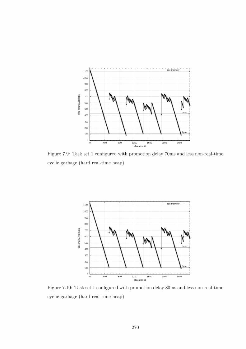
0

100

200

300

400

500

600

700

800

900

1000

1100

0 400 800 1200 1600 2000 2400

free

mem

ory(

bloc

ks)

allocation id

Lmax

Fpre

free memory



0

100

200

300

400

500

600

700

800

900

1000

1100

0 400 800 1200 1600 2000 2400

free

mem

ory(

bloc

ks)

allocation id

Lmax

Fpre

free memory



270

0

100

200

300

400

500

600

700

800

900

1000

1100

0 400 800 1200 1600 2000 2400

free

mem

ory(

bloc

ks)

allocation id

Lmax

Fpre

free memory

Figure 7.11: Task set 1 configured with promotion delay 0ms and more non-real-time


0

100

200

300

400

500

600

700

800

900

1000

1100

0 400 800 1200 1600 2000 2400

free

mem

ory(

bloc

ks)

allocation id

Lmax

Fpre

free memory

Figure 7.12: Task set 1 configured with promotion delay 10ms and more non-real-

time cyclic garbage (hard real-time heap)

271

0

100

200

300

400

500

600

700

800

900

1000

1100

0 400 800 1200 1600 2000 2400

free

mem

ory(

bloc

ks)

allocation id

Lmax

Fpre

free memory



0

100

200

300

400

500

600

700

800

900

1000

1100

0 400 800 1200 1600 2000 2400

free

mem

ory(

bloc

ks)

allocation id

Lmax

Fpre

free memory



272

0

100

200

300

400

500

600

700

800

900

1000

1100

0 400 800 1200 1600 2000 2400

free

mem

ory(

bloc

ks)

allocation id

Lmax

Fpre

free memory



0

100

200

300

400

500

600

700

800

900

1000

1100

0 400 800 1200 1600 2000 2400

free

mem

ory(

bloc

ks)

allocation id

Lmax

Fpre

free memory



273

0

200

400

600

800

1000

1200

1400

1600

1800

2000

2200

2400

2600

2800

0 800 1600 2400 3200 4000 4800 5600 6400 7200 8000 8800 9600 10400 11200

free

mem

ory(

bloc

ks)

allocation id

free memory


cyclic garbage (soft real-time heap)

0

200

400

600

800

1000

1200

1400

1600

1800

2000

2200

2400

2600

2800

0 800 1600 2400 3200 4000 4800 5600 6400 7200 8000 8800 9600 10400 11200

free

mem

ory(

bloc

ks)

allocation id

free memory



274

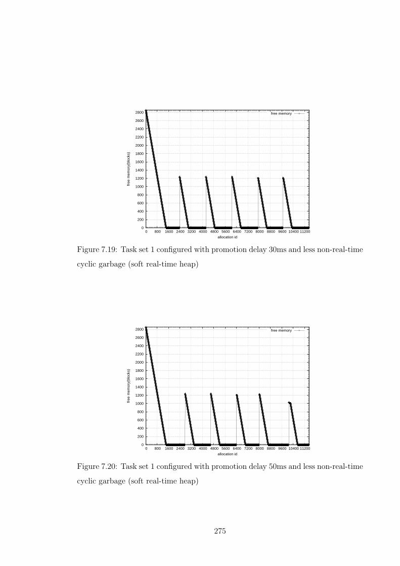
0

200

400

600

800

1000

1200

1400

1600

1800

2000

2200

2400

2600

2800

0 800 1600 2400 3200 4000 4800 5600 6400 7200 8000 8800 9600 10400 11200

free

mem

ory(

bloc

ks)

allocation id

free memory



0

200

400

600

800

1000

1200

1400

1600

1800

2000

2200

2400

2600

2800

0 800 1600 2400 3200 4000 4800 5600 6400 7200 8000 8800 9600 10400 11200

free

mem

ory(

bloc

ks)

allocation id

free memory



275

0

200

400

600

800

1000

1200

1400

1600

1800

2000

2200

2400

2600

2800

0 800 1600 2400 3200 4000 4800 5600 6400 7200 8000 8800 9600 10400 11200

free

mem

ory(

bloc

ks)

allocation id

free memory



0

200

400

600

800

1000

1200

1400

1600

1800

2000

2200

2400

2600

2800

0 800 1600 2400 3200 4000 4800 5600 6400 7200 8000 8800 9600 10400 11200

free

mem

ory(

bloc

ks)

allocation id

free memory



276

0

200

400

600

800

1000

1200

1400

1600

1800

2000

2200

2400

2600

2800

0 800 1600 2400 3200 4000 4800 5600 6400 7200 8000 8800 9600 10400 11200

free

mem

ory(

bloc

ks)

allocation id

free memory

Figure 7.23: Task set 1 configured with promotion delay 0ms and more non-real-time


0

200

400

600

800

1000

1200

1400

1600

1800

2000

2200

2400

2600

2800

0 800 1600 2400 3200 4000 4800 5600 6400 7200 8000 8800 9600 10400 11200

free

mem

ory(

bloc

ks)

allocation id

free memory


time cyclic garbage (soft real-time heap)

277

0

200

400

600

800

1000

1200

1400

1600

1800

2000

2200

2400

2600

2800

0 800 1600 2400 3200 4000 4800 5600 6400 7200 8000 8800 9600 10400 11200

free

mem

ory(

bloc

ks)

allocation id

free memory



0

200

400

600

800

1000

1200

1400

1600

1800

2000

2200

2400

2600

2800

0 800 1600 2400 3200 4000 4800 5600 6400 7200 8000 8800 9600 10400 11200

free

mem

ory(

bloc

ks)

allocation id

free memory



278

0

200

400

600

800

1000

1200

1400

1600

1800

2000

2200

2400

2600

2800

0 800 1600 2400 3200 4000 4800 5600 6400 7200 8000 8800 9600 10400 11200

free

mem

ory(

bloc

ks)

allocation id

free memory



0

200

400

600

800

1000

1200

1400

1600

1800

2000

2200

2400

2600

2800

0 800 1600 2400 3200 4000 4800 5600 6400 7200 8000 8800 9600 10400 11200

free

mem

ory(

bloc

ks)

allocation id

free memory



279

Cyclic Garbage P0 P10 P30 P50 P70 P80

Less 120179.2 117478.4 116832 117072 111705.6 112016

More 75248 75248 75248 78866.56 75248 76507.52

Table 7.1: The average amount of allocations (bytes) performed between two con-

secutive GC promotions (“Px” stands for “promotion delay x milliseconds”)

Notice, all these figures illustrate the amounts of remaining free memory after

the corresponding allocations. Therefore, the standard Java thread is not necessarily

blocked when zero free memory is observed in these figures. Moreover, even if the

standard Java thread is blocked, it could be resumed after a bounded and very

short duration because there could be enough acyclic (or recognised cyclic) garbage

for the soft reclaiming task to identify and reclaim. Therefore, a better way to

understand the memory availability and usage of the standard Java thread is to

observe the number of GC periods elapsed before a certain number of allocations

can be performed (that is, how fast an execution point of the standard Java thread

can be reached). For example, the executions configured with less cyclic garbage

usually use 4 - 5 GC periods to get to the point that usually costs 8 - 9 GC periods

when configured with more cyclic garbage. We can also use the average amount

of allocations performed between two consecutive GC promotions to measure the

memory availability and indicate the garbage collection progress (see table 7.1).

As illustrated by table 7.1, GC promotion delays have less influence on the free

memory changes of the soft- or non-real-time heap than the amount of cyclic garbage

in that heap. The more cyclic garbage exists, the less amount of allocations can be

performed between consecutive GC promotions, which results in longer time to reach

a certain execution point.

Moreover, some peaks in the figures 7.23, 7.24, 7.25, 7.26, 7.27 and 7.28 are

higher than the others. This is because the “soft-to-be-free-list” and the “soft-

white-list-buffer” have enough garbage when the soft reclaiming task is promoted.

Furthermore, the curves in the above figure sometimes grow horizontally (when

280

the free memory is not zero) because the promoted soft reclaiming task sometimes

reclaims the same amount of garbage as the next allocation requires. This is possible

because the promoted soft reclaiming task is suspended whenever both the “soft-

to-be-free-list” and the “soft-white-list-buffer” are empty while the standard Java

thread notifies the soft reclaiming task whenever it identifies a small amount of

acyclic garbage. If allocations always replace the same amount of live memory

(acyclic) and the above lists do not have other objects, the platforms appear in the

above figures.

7.5 Summary

In this chapter, a multi-heap approach was proposed to bound the soft- and non-real-

time tasks’ impacts on the memory usage and the schedulability of the hard real-time

tasks and still allow the soft- and non-real-time tasks’ flexible use of memory. The

algorithm as well as related rules, analyses and an automated program verification

prototype were presented.

Although certain reference assignment rules are required to be obeyed in our

system, they are significantly different with and less strict than those rules of RTSJ.

The differences are:

1. NoHeapRealtimeThread(s) in RTSJ are prohibited to access any reference to

heap, including static reference variables. On the other hand, our algorithm

only disallows to store references to the hard real-time heap in any field of

any object in the soft- or non-real-time heap. Any type of our user task can

access both heaps and even modify the object graphs of those heaps. The only

restriction is that a soft- or non-real-time task should never produce any cyclic

garbage in the hard real-time heap.

2. Read barriers are usually used by RTSJ implementations to enforce the afore-

mentioned access rules. In our system, an automated program verification

281

prototype is used to statically enforce one of our assignment rules. However,

the rule that soft- or non-real-time tasks should never produce any cyclic

garbage in the hard real-time heap cannot be automatically enforced in our

current implementation.

3. RTSJ requires to use write barriers to prohibit building certain references to

scoped memory areas. Such write barriers may result in unchecked exceptions

being thrown. On the other hand, our write barriers never fail.

Moreover, an implementation was introduced, which verifies the correctness and

efficiency of this approach. Discussions were also made on the WCETs of write

barriers, allocators and garbage collectors, as well as the worst-case blocking time

that could be encountered by tasks in the new system. Finally, a synthetic example

was demonstrated to show how such a system works and also the free memory

changes of both the hard and soft- or non-real-time heaps.

282

Chapter 8

Conclusions and Future Work

8.1 Meeting the Objectives

In chapter 1, we presented the hypothesis of this thesis:

• New design criteria are required for garbage collectors deployed in flexible

real-time systems with hard real-time constraints to better reflect the unique

characteristics and requirements of such systems. It is easier for the garbage

collectors that follow these criteria to achieve the correct balance between

temporal and spatial performance. It is also easier for a real-time system

that adopts such a garbage collector to improve the overall system utility and

performance (compared with real-time systems with other garbage collectors)

while still guaranteeing all the hard deadlines.

• It is practical to develop an algorithm which completely follows the guidance

of the new design criteria. It is also practical to fully implement such an

algorithm efficiently.

The primary goal of this research is to prove this hypothesis by: 1) proving

that new design criteria, particularly fine GC granularity and flexible scheduling

283

requirements, are crucial for the better design of new generation real-time garbage

collectors; 2) building an efficient real-time garbage collector that has fine GC gran-

ularities and better scheduling properties; 3) proving that the new collector gives

better chances to achieve the desired balance between temporal and spatial perfor-

mance; 4) proving that the scheduling of the proposed garbage collector improves

the overall system utility and performance while still guaranteeing all the hard dead-

lines.

In the last five chapters, we finished all these tasks and therefore proved our

hypothesis. Chapter 3 identified the key issues of the state-of-the-art real-time

garbage collectors and explained the fundamental cause of these issues. Therefore,

new design criteria were developed to highlight the directions of tackling these is-

sues. All these criteria reflect the unique characteristics and requirements of the

flexible real-time systems with hard real-time constraints. In particular, the con-

cept of GC granularity and a related performance indicator were proposed to quan-

titatively describe how easy a real-time garbage collector can achieve the correct

balance between temporal and spatial performance. Also, it was made clear that

more advanced scheduling approaches must be used for the new real-time garbage

collectors.

In chapter 4, a new hybrid garbage collection algorithm was designed completely

according to our design criteria. It is predictable because: 1) all the relevant prim-

itive operations have short and bounded execution times; 2) the garbage collector

is modeled as two periodic tasks, the WCETs of which can be predicted; 3) the

worst-case memory usage of the whole system can be derived a priori and alloca-

tion requests can always be satisfied. It is exact because enough type information

is available to the garbage collector so it can precisely identify roots and references

in the heap. It is complete because all the garbage objects can be identified and

reclaimed within a bounded time. Moreover, the new algorithm allows predictable

and fast preemptions because all the atomic operations in our algorithm are short

and bounded. The major sources of long atomic operations in modern garbage

284

collectors — root scanning, synchronization points and object copying — are elimi-

nated. The proposed collector degrades gracefully as well since it does not consume

any free memory during its execution (many other collectors, such as copying al-

gorithms, require free heap memory to proceed). More importantly, our garbage

collector has two dramatically different GC granularities, one of which is very low

while the other one is the same as the pure tracing collectors. By scheduling the two

GC tasks correctly, we successfully hide the impacts of the component with a high

GC granularity. Finally, the GC tasks are modeled as periodic real-time tasks so

different scheduling algorithms can be easily plugged in and the standard schedula-

bility analyses can be adopted as well. In the current development, the dual-priority

scheduling algorithm is chosen to help achieve the flexible scheduling required by

those flexible real-time systems with hard real-time requirements.

Chapter 5 provided the analyses required by our algorithm to guarantee all the

hard real-time deadlines and blocking-free allocations. Very little change has been

made to the standard response time analysis since our collector is well integrated

with the real-time scheduling framework.

In chapter 6, a prototype implementation of our algorithm was introduced. The

garbage collection algorithm has been completely implemented although there are a

few environmental limitations. Evaluations were performed to prove the efficiency

of our primitive operations and the claim that all the atomic operations are short

and bounded. Synthetic examples were also given to prove the effectiveness of the

whole system. In particular, the results were compared with a pure tracing system

and it was shown that our approach can better achieve the desired balance between

temporal and spatial performance. By investigating the response times of some

non-real-time tasks, it has also been proven that the proposed garbage collector

does not change the fact that a dual-priority scheduling system can improve the

overall system utility and performance.

Finally, chapter 7 relaxed some strict restrictions on the memory usage of the

soft- or non-real-time tasks. It has been proven that such changes do not jeopardize

285

any of the aforementioned properties.

8.2 Limitations and Future Work

Although our approach has been proven to be able to improve real-time garbage

collection in some key aspects, several issues have not been resolved. Solving these

problems forms the main parts of the future work.

First of all, relying on the reference counting algorithm to provide low GC gran-

ularity has some inherent limitations: 1) another algorithm has to be combined

with reference counting to identify cyclic garbage; 2) the accumulation of the write

barrier overheads could be very high because all the updates to the roots need to

be monitored and such operations are very frequent; and 3) an additional word is

used in each object (in many cases) to store the reference count(s). As a part of our

future work, experiments will be developed to investigate the overall costs of the

write barriers proposed in this thesis. The current difficulty of doing so is mainly

due to the lack of serious benchmark programs written in real-time Java. More

importantly, the future work will also include eliminating all the unnecessary write

barriers so that the overall costs of write barriers can be reduced. In particular,

we are interested in studying how the optimizations proposed by Ritzau [84] can be

performed in our system.

A possible alternative to the algorithm proposed in this thesis is to modify, ac-

cording to our design criteria, those tracing collectors that can perform incremental

reclamation, such as Harris and Hirzel et al.’s algorithms [50, 53]. Such a new al-

gorithm could have both the low GC granularity and the ability to reclaim all the

garbage. Therefore, a single collector with even less overhead could be developed to

satisfy our design criteria.

Although their worst-case GC granularities are still not as good as some refer-

ence counting algorithms, Harris and Hirzel et al.’s algorithms should be the most

286

promising ones of all the existing tracing algorithms because the garbage in each

(logical) heap partition can be identified and reclaimed independently. However,

work must be done to get even distributions of heap partitions, which is very diffi-

cult since the sizes of partitions are mainly determined by the applications. Also,

a new static analysis approach should be developed for such a collector to provide

hard real-time guarantees. In addition, better root scanning and defragmentation

techniques should be developed for this algorithm as well.

Although the data structures proposed in this thesis eliminate external fragmen-

tation and allow efficient cooperation between reference counting and tracing, there

are still a few problems: 1) three additional words are required in each object header,

which are heavy per-object memory overheads; 2) links have to be maintained be-

tween different blocks of the same object, which introduces memory overheads as

well; 3) accessing an object/array field is potentially expensive; and 4) internal frag-

mentation may be significant in some applications, under specific configurations.

As discussed in chapter 4, choosing the right size for memory blocks is key to lower

memory access overheads as well as lower internal fragmentations. Therefore, fur-

ther efforts could be made to check whether 32 bytes are still the best choice for

the block size (recall that 32 bytes are the result of Siebert’s study [92, 94] and our

object/array header size is different). In order to reduce the spatial and temporal

overheads of organizing those very large arrays as trees, a conventional heap could

be introduced to store such arrays in a traditional way. However, this heap must

be managed separately and the compiler should generate different code for different

array accesses. Moreover, different data structures (and perhaps algorithms) could

be tried to reduce the per-object memory overheads while still allowing our other

goals to be achieved.

Currently, we assume that the maximum amount of cyclic garbage introduced

by each release of each hard real-time user task is always known. In the synthetic

examples demonstrated in this thesis, the cyclic garbage is deliberately maintained

at such amounts. A method to automatically derive such information from any given

287

user application is going to be very important for the success of our approach in the

real world. Although the exact maximum amount of cyclic garbage introduced by

each release of each hard real-time user task may be very difficult to obtain, safe

and tight estimations should be able to achieve. In the future, it could be tried

to combine the class hierarchy analysis proposed by Harris [50], Java generics [47]

and automated program verification tools such as the Java PathFinder [51, 104], to

accurately identify all the classes that could be used to build cyclic structures in

each task. Then, an approximation of the maximum amount of cyclic garbage could

possibly be deduced on the basis of the above information.

Moreover, the current WCET estimation of our garbage collector is not very

tight. There is too much pessimism because of the missing crucial information

such as real reference intensity, the amount of memory managed by the “white-list-

buffer”, the number of objects directly referenced by roots, the maximum number of

objects that occupy no more than Lmax +2 ·CGGmax and the number of blocks that

have no reference field at all. Thus, work could be done to achieve such information

and develop a new WCET estimation approach which uses such information to get

tighter results.

In chapter 5, it was assumed that all the hard real-time user tasks are completely

independent of each other. All of our static analyses are built on this assumption.

However, this is not usually the case in real applications. The future work could

include the development of new static analyses that take resource sharing into con-

sideration. The static analysis proposed along with the dual-priority scheduling

algorithm has already included the blocking factors. However, it cannot be directly

used in our algorithm because user tasks with lower priorities than the GC tasks

could inherit a priority even higher than the GC tasks (when they are trying to

lock a resource that could be shared between it and a high priority user task or

a high priority user task is trying to lock a resource that has been locked by the

aforementioned low priority task, depending on which protocol is used). This does

not only delay the execution of the GC tasks, but also introduce more allocations

288

with higher priorities than the GC tasks since the memory allocated by the low

priority user tasks running at inherited high priorities is not expected in the current

analyses. Such behaviour has an impact on the estimation of Fpre. Work could be

done to model this impact. Moreover, the GC tasks could suffer more than one of

such hits because the reclaiming task could be suspended waiting for garbage during

a release. Work should be done to better understand this impact as well.

Furthermore, evaluations should also be performed to examine the effectiveness

and efficiency of our approach when arrays are present. In particular, evaluating

our system on serious benchmark programs (written in real-time Java) could give a

more practical view and a better understanding of our algorithm.

We are also interested in studying how to use runtime information to better

schedule our garbage collector. For example, we could modify the scheduler so that

it increases the initial GC promotion delay if extra reclamation has been performed

in the previous GC period (currently, we reduce the work amount limit on the

reclaiming task if extra reclamation has been performed).

Future research could also include an investigation on the temporal and spa-

tial locality of our garbage collector as well as a study on taking advantage of the

multicore processors (which are very common nowadays) to develop better garbage

collectors.

Finally, the prototype implementation should be further improved as well. For

example, we could modify all the hard real-time user tasks so that they are also

scheduled according to the dual-priority algorithm (subsequently, we would test the

response times of the non-real-time tasks again.); the bootstrap heap (see chapter

6) will be merged with the garbage collected heap eventually; efforts could be made

to port the whole system on a stand-alone MaRTE OS so that synchronization costs

can be reduced and true real-time performance can be guaranteed; exceptions, final-

izers and reference objects could be added in a way that can still provide real-time

guarantees; work could also be done to fully implement the scheduling algorithm

289

(priority inheritance) proposed for the execution of the soft reclaiming task in the

middle priority band; a static analysis tool or a runtime mechanism could be devel-

oped to automatically enforce the rule that no soft- or non-real-time task produce

any cyclic garbage in the hard real-time heap (currently, it is programmers’ respon-

sibility to make sure that this rule is never violated).

8.3 In Conclusion

The research presented in this thesis highlights some criteria that real-time garbage

collector design should follow. Garbage collectors designed according to such criteria

are expected to better suit the flexible real-time systems with hard real-time require-

ments. As the first example of such a garbage collector, our algorithm is proven to

be effective. In particular, it helps achieve the desired performance balance and

better scheduling of the whole system.

The proposed criteria also represent some key directions of future real-time

garbage collection research. For example, developing new algorithms to achieve

finer worst-case GC granularities and integrating such algorithms with advanced

real-time scheduling frameworks are both interesting topics. Also, exact root scan-

ning, incremental root scanning and interruptible object copying all require better

solutions. We also believe that static program analysis, multiprocessor (or multicore

processor) garbage collection and hardware garbage collection should help result in

even more capable real-time garbage collectors.

Real-time garbage collection is still not mature for demanding real-time systems

with tens of microseconds response time requirements. Meanwhile, the existing dy-

namic memory management approaches adopted in real-time systems cannot provide

as much software engineering benefit as garbage collection. Therefore, the search for

better automatic dynamic memory model suitable for real-time systems continues.

290

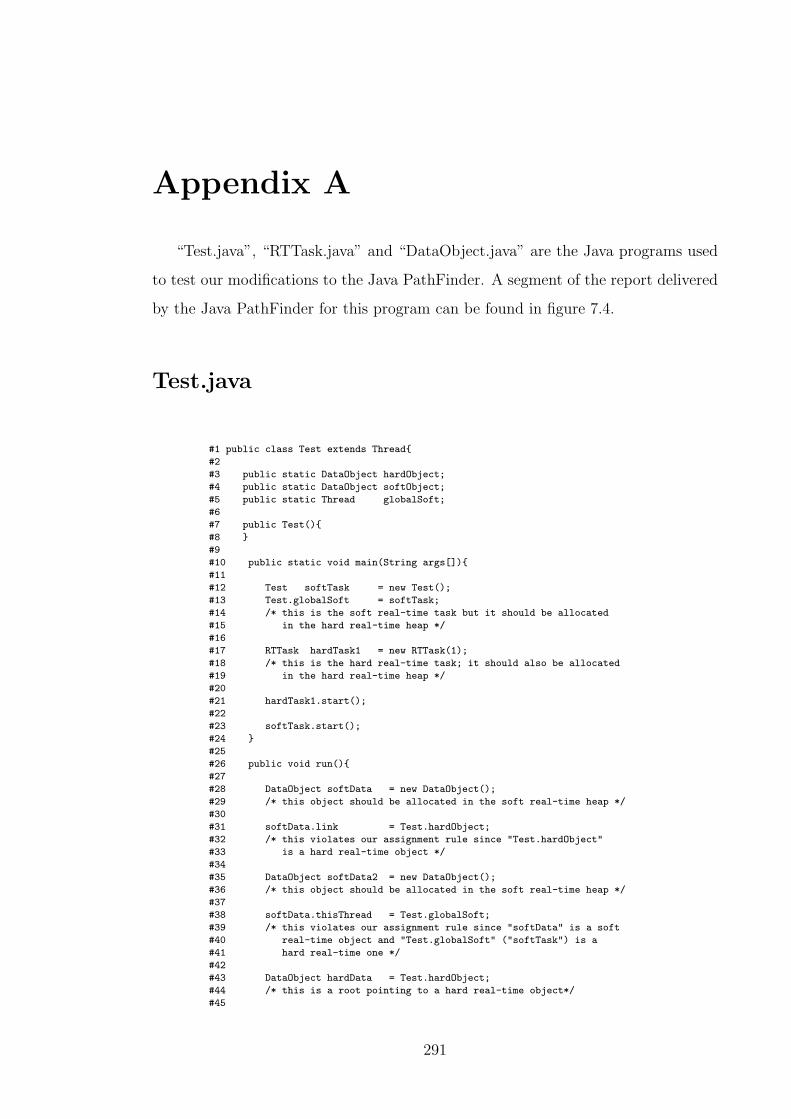
Appendix A

“Test.java”, “RTTask.java” and “DataObject.java” are the Java programs used

to test our modifications to the Java PathFinder. A segment of the report delivered

by the Java PathFinder for this program can be found in figure 7.4.

Test.java

#1 public class Test extends Thread{

#2

#3 public static DataObject hardObject;

#4 public static DataObject softObject;

#5 public static Thread globalSoft;

#6

#7 public Test(){

#8 }

#9

#10 public static void main(String args[]){

#11

#12 Test softTask = new Test();

#13 Test.globalSoft = softTask;

#14 /* this is the soft real-time task but it should be allocated

#15 in the hard real-time heap */

#16

#17 RTTask hardTask1 = new RTTask(1);

#18 /* this is the hard real-time task; it should also be allocated

#19 in the hard real-time heap */

#20

#21 hardTask1.start();

#22

#23 softTask.start();

#24 }

#25

#26 public void run(){

#27

#28 DataObject softData = new DataObject();

#29 /* this object should be allocated in the soft real-time heap */

#30

#31 softData.link = Test.hardObject;

#32 /* this violates our assignment rule since "Test.hardObject"

#33 is a hard real-time object */

#34

#35 DataObject softData2 = new DataObject();


#37

#38 softData.thisThread = Test.globalSoft;

#39 /* this violates our assignment rule since "softData" is a soft

#40 real-time object and "Test.globalSoft" ("softTask") is a

#41 hard real-time one */

#42

#43 DataObject hardData = Test.hardObject;

#44 /* this is a root pointing to a hard real-time object*/

#45

291

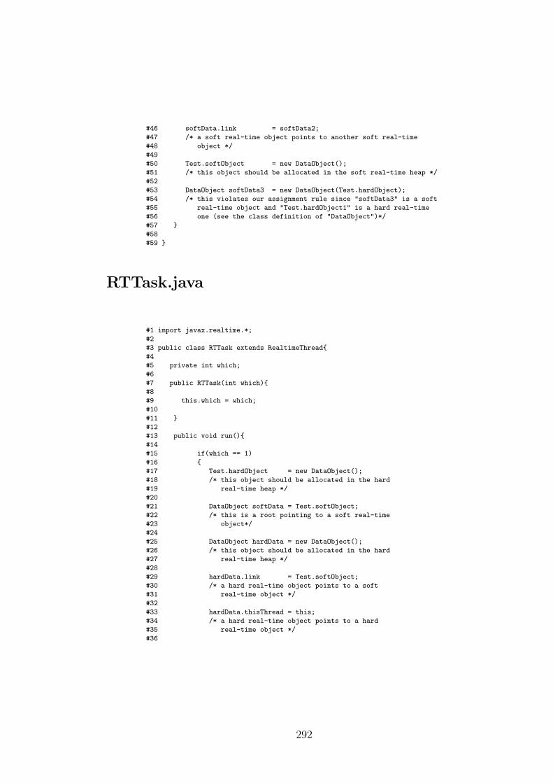
#46 softData.link = softData2;

#47 /* a soft real-time object points to another soft real-time

#48 object */

#49

#50 Test.softObject = new DataObject();


#52

#53 DataObject softData3 = new DataObject(Test.hardObject);

#54 /* this violates our assignment rule since "softData3" is a soft

#55 real-time object and "Test.hardObject1" is a hard real-time

#56 one (see the class definition of "DataObject")*/

#57 }

#58

#59 }

RTTask.java

#1 import javax.realtime.*;

#2

#3 public class RTTask extends RealtimeThread{

#4

#5 private int which;

#6

#7 public RTTask(int which){

#8

#9 this.which = which;

#10

#11 }

#12


#14

#15 if(which == 1)

#16 {

#17 Test.hardObject = new DataObject();

#18 /* this object should be allocated in the hard

#19 real-time heap */

#20

#21 DataObject softData = Test.softObject;

#22 /* this is a root pointing to a soft real-time

#23 object*/

#24

#25 DataObject hardData = new DataObject();

#26 /* this object should be allocated in the hard

#27 real-time heap */

#28

#29 hardData.link = Test.softObject;

#30 /* a hard real-time object points to a soft

#31 real-time object */

#32

#33 hardData.thisThread = this;

#34 /* a hard real-time object points to a hard


#36

292

#37 hardData.link = hardData;



#40

#41 hardData.thisThread = Test.globalSoft;



#44

#45 }

#46 }

#47

#48 }

DataObject.java

#1 public class DataObject{

#2

#3 public Thread thisThread;

#4 public DataObject link;

#5 private int dataMember;

#6

#7 public DataObject(){

#8

#9 thisThread = null;

#10 link = null;

#11 dataMember = 0;

#12

#13 }

#14

#15 public DataObject(DataObject par){

#16

#17 thisThread = null;

#18

#19 link = par;

#20 /*this may violate our assignment rule*/

#21

#22 dataMember = 0;

#23

#24 }

#25 }

293

Appendix B

“SoftTask.java” and “DataTest.java” are the Java files needed to run a non-

real-time task (with flexible memory usage) to investigate the temporal and spatial

performances of our algorithms proposed in chapter 7. All the evaluations presented

in that chapter are based on the code below:

SoftTask.java

#1 public class SoftTask extends Thread{

#2

#3 int whichOne;

#4

#5 public SoftTask(){

#6 }

#7

#8 public SoftTask(int i){

#9 whichOne = i;

#10 }

#11


#13

#14 if(whichOne == 1){

#15

#16 DataTest begin = null;

#17 DataTest end = null;

#18

#19 int i=0;

#20

#21 for(; i<650; i++)

#22 {

#23 if( begin == null ){

#24

#25 begin = new DataTest();

#26 end = begin;

#27 }

#28 else{

#29

#30 end.a5 = new DataTest();

#31 end = end.a5;

#32 }

#33 }

#34

#35 ExperimentSoft.globalEnd.a5 = begin;

#36 /* a hard real-time object referenced by "globalEnd"

#37 references the head of the above link */

#38

#39 begin = end = null;

#40 /* clear all the other references to this link */

#41

#42 for(i=0; i<650; i++)

#43 {

294

#44 if( begin == null ){

#45

#46 begin = new DataTest();

#47 end = begin;

#48 }

#49 else{

#50

#51 end.a5 = new DataTest();

#52 end = end.a5;

#53 }

#54 }

#55

#56 ExperimentSoft.hardRoot = begin;

#57 /* a static reference variable, "hardRoot", references

#58 the head of the above link */

#59

#60 begin = end = null;

#61 /* clear all the other references to this link */

#62

#63 ExperimentSoft.globalEnd = null;

#64 /* clear all the roots that points to the hard real-time

#65 object that references the first link created in this

#66 method */

#67

#68 ExperimentSoft.globalPre.a5 = null;

#69 /* clear all the other references that points to the hard

#70 real-time object that references the first link created

#71 in this method */

#72

#73 while(true){

#74

#75 int j=0;

#76

#77 for( ; j<=10500; j++ )

#78 {

#79 double z = 3.1415926;

#80 double x = 100000;

#81 x = x/z;

#82 }

#83

#84 System.out.println("Hello World");

#85

#86 for(j=0; j<50; j++)

#87 {

#88 DataTest first = new DataTest();

#89 first.a5 = new DataTest();

#90 }

#91 /* these are acyclic garbage */

#92

#93 for(j=0; j<=10500; j++)

#94 {

#95 double z = 3.1415926;

#96 double x = 100000;

#97 x = x/z;

#98 }

#99

#100 for(j=0; j<20; j++)

#101 /* when configured to generate less cyclic garbage,

#102 substitute 20 with 45 */

#103 {



#106 }

#107 /* these are acyclic garbage */

#108

295

#109 for(j=0; j<30; j++)

#110 /* when configured to generate less cyclic garbage,

#111 substitute 30 with 5 */

#112 {



#115 first.a5.a5 = first;

#116 }

#117 /* these are cyclic garbge */

#118 }

#119 }

#120 else{

#121 while(true);

#122 }

#123 }

#124}

DataTest.java

#1 import gnu.gcj.RawData;

#2

#3 public class DataTest{

#4

#5 long a1;

#6 int a;

#7 int a2;

#8 int a4[];

#9 public DataTest a5;

#10 DataTest a6[];

#11 RawData rwd;

#12

#13 public DataTest(){

#14 }

#15

#16 public DataTest( DataTest value ){

#17

#18 a = value.a;

#19 a1 = value.a1;

#20 a2 = value.a2;

#21 a4 = value.a4;

#22 a5 = value.a5;

#23 a6 = value.a6;

#24 rwd = value.rwd;

#25

#26 }

#27

#28 public void testFun1(){

#29 }

#30

#31 public DataTest testFun2(){

#32

#33 return a5;

#34 }

#35


#37

#38 DataTest x = new DataTest();

#39 return x;

#40 }

#41

296


#43

#44 return new DataTest();

#45 }

#46


#48

#49 return testFun4();

#50 }

#51


#53

#54 return testFun3();

#55 }

#56

#57 public void testFun7(DataTest x){

#58

#59 a5 = x;

#60 }

#61 }

297

Bibliography

[1] Santosh Abraham and Janak Patel. Parallel garbage collection on a virtual

memory system. In Proceedings of the International Conference on Parallel

Processing, pages 243–246, 1987.

[2] Ole Agesen and David Detlefs. Finding references in Java stacks. In Proceed-

ings of OOPSLA97 Workshop on Garbage Collection and Memory Manage-

ment, pages 766–770, 1997.

[3] Ole Agesen, David Detlefs, and Eliot Moss. Garbage collection and local

variable type-precision and liveness in Java virtual machines. In Proceedings

of ACM SIGPLAN 1998 PLDI, pages 269–279, 1998.

[4] Andrew W. Appel. Runtime tags aren’t necessary. LISP and Symbolic Com-

putation, 2(2):153–162, 1989.

[5] Andrew W. Appel. Simple generational garbage collection and fast allocation.

Software Practice and Experience, 19(2):171–183, 1989.

[6] Neil Audsley, Alan Burns, M. Richardson, K. Tindell, and Andy Wellings. Ap-

plying new scheduling theory to static priority pre-emptive scheduling. Soft-

ware Engineering Journal, 8(5):284–292, 1993.

[7] Neil C. Audsley. Flexible Scheduling in Hard Real-Time Systems. PhD thesis,

University of York, 1993.

298

[8] Hezi Azatchi, Yossi Levanoni, Harel Paz, and Erez Petrank. An on-the-fly

mark and sweep garbage collector based on sliding views. In Proceedings of

the 18th OOPSLA, pages 269–281, 2003.

[9] David F. Bacon, Perry Cheng, and V.T. Rajan. Controlling fragmentation

and space consumption in the Metronome, a real-time garbage collector for

Java. In Proceedings of the ACM SIGPLAN 2003 Conference on Language

Design, Compiler, and Tool for Embedded Systems, pages 81–92, 2003.

[10] David F. Bacon, Perry Cheng, and V.T. Rajan. The Metronome: A simpler

approach to garbage collection in real-time systems. In Proceedings of OTM

2003 Workshops, pages 466–478, 2003.

[11] David F. Bacon, Perry Cheng, and V.T. Rajan. A real-time garbage collector

with low overhead and consistent utilization. In Proceedings of POPL 2003,

pages 285–298, 2003.

[12] David F. Bacon and V.T. Rajan. Concurrent cycle collection in reference

counted systems. In Proceedings of the 15th European Conference on Object-

Oriented Programming, pages 207–235, 2001.

[13] Henry G. Baker. List processing in real time on a serial computer. Commu-

nications of the ACM, 21(4):280–294, 1978.

[14] Henry G. Baker. The Treadmill: Real-time garbage collection without motion

sickness. ACM Sigplan Notices, 27(3):66–70, 1992.

[15] Guillem Bernat and Alan Burns. New results on fixed priority aperiodic

servers. In Proceedings of the IEEE Real-Time Systems Symposium, pages

68–78, 1999.

[16] Bruno Blanchet. Escape analysis for object oriented languages: Application

to Java. In Proceedings of OOPSLA’99, pages 20–34, 1999.

299

[17] Hans-J. Boehm. Bounding space usage of conservative garbage collectors. In

Proceedings of the 29th ACM SIGPLAN-SIGACT Symposium on Principles

of Programming Languages, pages 93–100, 2002.

[18] Hans-J. Boehm. The space cost of lazy reference counting. In Proceedings of

the 31st ACM SIGPLAN-SIGACT Symposium on Principles of Programming

Languages, pages 210–219, 2004.

[19] Hans-J. Boehm and Mark Weiser. Garbage collection in an uncooperative

environment. Software Practice and Experience, 18(9):807–820, 1988.

[20] G. Bollella, B. Brosgol, P. Dibble, S. Furr, J. Gosling, D. Hardin, M. Turnbull,

and R. Belliardi. The Real-Time Specification for Java (1.0). Addison Wesley,

2001.

[21] Andrew Borg, Andy Wellings, Christopher Gill, and Ron K. Cytron. Real-time

memory management: Life and times. In Proceedings of the 18th Euromicro,

pages 237–250, 2006.

[22] P. Branquart and J. Lewi. A scheme of storage allocation and garbage col-

lection for ALGOL 68. In Proceedings of the IFIP Working Conference on

ALGOL 68 Implementation, pages 199–232, 1970.

[23] Rodney A. Brooks. Trading data space for reduced time and code space in

real-time garbage collection on stock hardware. In Proceedings of the 1984

ACM Symposium on LISP and functional programming, pages 256–262, 1984.

[24] Alan Burns and Andy Wellings. Real-Time Systems and Programming Lan-

guages. Addison Wesley, third edition, 2001.

[25] Dante J. Cannarozzi, Michael P.Plezbert, and Ron K. Cytron. Contaminated

garbage collection. In Proceedings of PLDI 2000, pages 264–273, 2000.

[26] Yang Chang. Application level memory management for real-time systems.

Technical report, University of York, 2004.

300

[27] Yang Chang. Integrating hybrid garbage collection with dual prior-

ity scheduling. Technical Report YCS 388, University of York, 2005.

http://www.cs.york.ac.uk/ftpdir/reports/YCS-2005-388.pdf.

[28] Yang Chang. Hard real-time hybrid garbage collection with low memory

requirement. Technical Report YCS-2006-403, University of York, 2006.

http://www.cs.york.ac.uk/ftpdir/reports/YCS-2006-403.pdf.

[29] Yang Chang and Andy Wellings. Integrating hybrid garbage collection with

dual priority scheduling. In Proceedings of the 11th IEEE International Con-

ference on Embedded and Real-Time Computing Systems and Applications,

pages 185–188, 2005.

[30] Yang Chang and Andy Wellings. Hard real-time hybrid garbage collection

with low memory requirements. In Proceedings of the 27th IEEE Real-Time

Systems Symposium, pages 77–86, 2006.

[31] Yang Chang and Andy Wellings. Low memory overhead real-time garbage

collection for Java. In Proceedings of the 4th International Workshop on Java

Technologies for Real-Time and Embedded Systems, pages 85–94, 2006.

[32] C. J. Cheney. A non-recursive list compacting algorithm. Communications of

the ACM, 13(11):677–678, 1970.

[33] Thomas W. Christopher. Reference count garbage collection. Software-Pratice

and Experience, 14(6):503–507, 1984.

[34] George E. Collins. A method for overlapping and erasure of lists. Communi-

cations of the ACM, 3(12):655–657, 1960.

[35] Angelo Corsaro and Douglas C. Schmidt. The design and performance of the

JRate real-time Java implementation. In Proceedings of the 4th International

Symposium on Distributed Objects and Applications, pages 900–921, 2002.

301

[36] Robert Davis and Andy Wellings. Dual priority scheduling. In Proceedings of

the 16th IEEE Real-Time Systems Symposium, pages 100–109, 1995.

[37] Robert Ian Davis. On Exploiting Spare Capacity in Hard Real-Time Systems.

PhD thesis, The University of York, 1995.

[38] John DeTreville. Experience with concurrent garbage collectors for Modula-

2+. Technical Report 64, DEC Systems Research Center, Palo Alto, CA,

1990.

[39] L. Peter Deutsch and Daniel G. Bobrow. An efficient incremental automatic

garbage collector. Communications of the ACM, 19(9):522–526, 1976.

[40] Edsger W. Dijkstra, Leslie Lamport, A.J. Martin, C.S. Scholten, and E.F.M.

Steffens. On-the-fly garbage collection: An exercise in cooperation. CACM,

21(11):966–975, 1978.

[41] Amer Diwan, Eliot Moss, and Richard Hudson. Compiler support for garbage

collection in a statically typed language. In Proceedings of ACM SIGPLAN

1992 PLDI, pages 273–282, 1992.

[42] A. Dix, R.F. Stone, and H.Zedan. Design issues for reliable time-critical sys-

tems. In Proceedings of the Real-Time Systems: Theory and Applications, ed.

H. Zedan, North Holland, pages 305–322, 1989.

[43] Robert R. Fenichel and Jerome C. Yochelson. A LISP garbage-collector for

virtual-memory computer systems. Comunications of the ACM, 12(11):611–

612, 1969.

[44] David Gay and Alex Aiken. Memory management with explicit regions. In

Proceedings of PLDI 1998, pages 313–323, 1998.

[45] David Gay and Bjarne Steensgaard. Fast escape analysis and stack allocation

for object-based programs. In Proceedings of the 2000 International Confer-

ence on Compiler Construction, 2000.

302

[46] Benjamin Goldberg. Tag-free garbage collection for strongly typed program-

ming languages. In Proceedings of the ACM SIGPLAN 1991 Conference on

Programming Language Design and Implementation, pages 165–176, 1991.

[47] James Gosling, Bill Joy, Guy Steele, and Gilad Bracha. The Java Language

Specification. Prentice Hall PRT, third edition, 2005.

[48] Object Management Group. Real-Time CORBA Specification. Technical Re-

port formal/02-08-02, OMG, 2002.

[49] Niels Hallenberg, Martin Elsman, and Mads Tofte. Combining region inference

and garbage collection. ACM SIGPLAN Notices, 37(5):141–152, 2002.

[50] Timothy Harris. Early storage reclamation in a tracing garbage collector.

ACM SIGPLAN Notices, 34(4):46–53, 1999.

[51] K. Havelund and T. Pressburger. Model checking Java programs using Java

PathFinder. International Journal on Software Tools for Technology Transfer,

2(4):366–381, 2000.

[52] Roger Henriksson. Scheduling Garbage Collection in Embedded Systems. PhD

thesis, Lund University, 1998. http://www.cs.lth.se/home/Roger Henriksson

/thesis.pdf.

[53] Martin Hirzel, Amer Diwan, and Matthew Hertz. Connectivity-based garbage

collection. In Proceedings of the 18th ACM SIGPLAN Conference on Object-

Oriented Programing, Systems, Languages and Applications, pages 359–373,

2003.

[54] IEEE. ISO/IEC Standard 9945-1:1996. Information Technology–Portable Op-

erating System Interface (POSIX)–Part 1: System Application Program In-

terface (API) [C Language].

303

[55] Mark S. Johnstone and Paul R. Wilson. The memory fragmentation problem:

Solved? In Proceedings of the International Symposium on Memory Manage-

ment, pages 26–36, 1998.

[56] Mark Stuart Johnstone. Non-Compacting Memory Allocation and Real-Time

Garbage Collection. PhD thesis, The University of Texas at Austin, 1997.

[57] Richard Jones and Rafael Lins. Garbage Collection. John Wiley & Sons, 1996.

[58] Taehyoun Kim, Naehyuck Chang, Namyun Kim, and Heonshik Shin. Schedul-

ing garbage collection for embedded real-time systems. In Workshop on Lan-

guages, Compilers and Tools for Embedded Systems, pages 55–64, 1999.

[59] Taehyoun Kim, Naehyuck Chang, and Heonshik Shin. Bounding worst case

garbage collection time for embedded real-time systems. In Proceedings of the

6th IEEE RTAS, pages 46–55, 2000.

[60] Taehyoun Kim, Naehyuck Chang, and Heonshik Shin. Joint scheduling of

garbage collector and hard real-time tasks for embedded applications. Journal

of Systems and Software, 58(3):247–260, 2001.

[61] Taehyoun Kim and Heonshik Shin. Scheduling-aware real-time garbage col-

lection using dual aperiodic servers. In Proceedings of the IEEE 9th RTCSA,

pages 3–20, 2003.

[62] John P. Lehoczky and Sandra Ramos-Thuel. An optimal algorithm for schedul-

ing soft-aperiodic tasks in fixed-priority pre-emptive systems. In Proceedings

of the IEEE Real-Time Systems Symposium, pages 110–123, 1992.

[63] John P. Lehoczky, L. Sha, and J. K. Strosnider. Enhanced aperiodic respon-

siveness in a hard real-time environment. In Proceedings of the IEEE Real-

Time Systems Symposium, pages 261–270, 1987.

304

[64] J. Leung and J. Whitehead. On the complexity of fixed-priority scheduling of

periodic, real-time tasks. Performance Evaluation(Netherlands), 2(4):237–250,

1982.

[65] Yossi Levanoni and Erez Petrank. An on-the-fly reference-counting garbage

collector for Java. ACM Transactions on Programming Languages and Sys-

tems, 28(1):1–69, 2006.

[66] Henry Lieberman and Carl Hewitt. A real-time garbage collector based on the

lifetimes of objects. Communications of the ACM, 26(6):419–429, 1983.

[67] Tim Lindholm and Frank Yellin. The Java Virtual Machine Specification.

Prentice Hall PRT, second edition, 1999.

[68] Rafael D. Lins. Cyclic reference counting with lazy mark-scan. Information

Processing Letters, 44(4):215–220, 1992.

[69] C. L. Liu and James W. Layland. Scheduling algorithms for multiprogramming

in a hard-real-time environment. JACM, 20(1):46–61, 1973.

[70] S. Marshall. An ALGOL 68 garbage collector. In Proceedings of the IFIP

Working Conference on ALGOL 68 Implementation, pages 239–243, 1970.

[71] A. D. Martinez, R. Wachenchauzer, and Rafael D. Lins. Cyclic reference

counting with local mark-scan. Information Processing Letters, pages 31–35,

1990.

[72] Miguel Masmano, Ismael Ripoll, and Alfons Crespo. A comparison of memory

allocators for real-time applications. In Proceedings of the 4th International

Workshop on Java Technologies for Real-time and Embedded Systems, pages

68–76, 2006.

[73] J. Harold McBeth. On the reference counter method. Communications of the

ACM, 6(9):575, 1963.

305

[74] John McCarthy. Recursive functions of symbolic expressions and their com-

putation by machine. Communications of the ACM, 3(4):184–195, 1960.

[75] S. Nettles and J. O’Toole. Real-time replication garbage collection. In Pro-

ceedings of the ACM SIGPLAN 1993 Conference on Programming Language

Design and Implementation, pages 217–226, 1993.

[76] K.D. Nilsen and W.J. Schmidt. A high-performance hardware assisted real-

time garbage collection system. Journal of Programming Languages, 2(1):1–40,

1994.

[77] David Patterson, Thomas Anderson, Neal Cardwell, Richard Fromm, Kim-

berly Keeton, Christoforos Kozyrakis, Randi Thomas, and Katherine Yelick.

A case for intelligent RAM. IEEE Micro, 17(2):34–44, 1997.

[78] Rasmus Pedersen and Martin Schoeberl. Exact roots for a real-time garbage

collector. In Proceedings of the 4th International Workshop on Java Technolo-

gies for Real-time and Embedded Systems, pages 77–84, 2006.

[79] Pekka P. Pirinen. Barrier techniques for incremental tracing. In Proceedings

of the International Symposium on Memory Management, pages 20–25, 1998.

[80] F. Pizlo, J. M. Fox, D. Holmes, and J. Vitek. Real-time Java scoped memory:

Design patterns and semantics. In Proceedings of ISORC 2004, pages 101–110,

2004.

[81] Feng Qian and Laurie Hendren. An adaptive, region-based allocator for

Java. In Proceedings of the International Symposium on Memory Manage-

ment, pages 127–138, 2002.

[82] Sandra Ramos-Thuel and John P. Lehoczky. On-line scheduling of hard dead-

line aperiodic tasks in fixed-priority systems. In Proceedings of the IEEE

Real-Time Systems Symposium, pages 160–171, 1993.

306

[83] Tobias Ritzau. Hard real-time reference counting without external fragmen-

tation. In Java Optimization Strategies for Embedded Systems Workshop at

ETAPS, 2001.

[84] Tobias Ritzau. Memory Efficient Hard Real-Time Garbage Collection. PhD

thesis, Linkoping University, 2003.

[85] Mario Aldea Rivas and Michael Gonzlez Harbour. MaRTE OS: An Ada kernel

for real-time embedded applications. In Ada-Europe, pages 305–316, 2001.

[86] Sven Gestegard Robertz. Applying priorities to memory allocation. In Proceed-

ings of the International Symposium on Memory Management, pages 108–118,

2003.

[87] Sven Gestegard Robertz and Roger Henriksson. Time-triggered garbage

collection—robust and adaptive real-time gc scheduling for embedded systems.

In Proceedings of LCTES 2003, pages 93–102, 2003.

[88] L. Sha, J. P. Lehoczky, and R. Rajkumar. Solutions for some practical prob-

lems in prioritised preemptive scheduling. In Proceedings of the IEEE Real-

Time Systems Symposium, pages 181–191, 1986.

[89] Fridtjof Siebert. Guaranteeing non-disruptiveness and real-time deadlines in

an incremental garbage collector. In Proceedings of the first international

symposium on Memory management, pages 130–137, 1998.

[90] Fridtjof Siebert. Hard real-time garbage collection in the Jamaica virtual ma-

chine. In Proceedings of 6th International Conference on Real-Time Computing

Systems and Applications, pages 96–102, 1999.

[91] Fridtjof Siebert. Real-time garbage collection in multi-threaded systems on a

single processor. In Proceedings of 20th IEEE Real-Time Systems Symposium,

page 277, 1999.

307

[92] Fridtjof Siebert. Eliminating external fragmentation in a non-moving garbage

collector for Java. In Compilers, Architectures and Synthesis for Embedded

systems(CASES2000), pages 9–17, 2000.

[93] Fridtjof Siebert. Constant-time root scanning for deterministic garbage collec-

tion. In Proceedings of the 10th International Conference on Compiler Con-

struction, pages 304–318, 2001.

[94] Fridtjof Siebert. Hard Real Time Garbage Collection in Modern Ojbect Ori-

ented Programming Languages. PhD thesis, University of Karlsruhe, 2002.

[95] Fridtjof Siebert. The impact of realtime garbage collection on realtime Java

programming. In Proceedings of ISORC 2004, pages 33–40, 2004.

[96] B. Sprunt, J. Lehoczky, and L. Sha. Exploiting unused periodic time for ape-

riodic service using the extended priority exchange algorithm. In Proceedings

of the IEEE Real-Time Systems Symposium, pages 251–258, 1988.

[97] John A. Stankovic, Marco Spuri, and Krithi Ramamritham. Deadline Schedul-

ing for Real-Time Systems-EDF and Related Algorithms. 1998.

[98] Guy L. Steele. Multiprocessing compactifying garbage collection. Communi-

cations of the ACM, 18(9):495–508, 1975.

[99] James M. Stichnoth, Guei-Yuan Lueh, and Michal Cierniak. Support for

garbage collection at every instruction in a Java compiler. ACM SIGPLAN

Notices, 34(5):118–127, 1999.

[100] Robert Endre Tarjan. Efficiency of a good but not linear set union algorithm.

The Association for Computing Machinery, 22(2):215–225, 1975.

[101] Mads Tofte and Jean-Pierre Talpin. Region-based memory management. In-

formation and Computation, 132(2):109–176, 1997.

308

[102] David Ungar. Generation scavenging: A non-disruptive high performance

storage reclamation algorithm. ACM SIGPLAN Notices, 19(5):157–167, 1984.

[103] Martin T. Vechev and David F. Bacon. Write barrier elision for concurrent

garbage collectors. In Proceedings of ISMM 2004, pages 13–24, 2004.

[104] W. Visser, K. Havelund, G. Brat, and S. Park. Model checking programs.

Automated Software Engineering Journal, 10(2):203–232, 2003.

[105] Nelson H. Weiderman and Nick I. Kamenoff. Hartstone uniprocessor bench-

mark: Definitions and experiments for real-time systems. Real-Time Systems,

4(4):353–382, 1992.

[106] J. Weizenbaum. Symmetric list processor. Communications of the ACM,

6(9):524–544, 1963.

[107] Andy Wellings, Ray Clark, Doug Jensen, and Doug Wells. A framework for in-

tegrating the Real-Time Specification for Java and Java’s Remote Method In-

vocation. In Proceedings of the 5th IEEE International Symposium on Object-

Oriented Real-Time Distributed Computing, pages 13–22, 2002.

[108] Paul R. Wilson. Uniprocessor garbage collection techniques. In Proceedings

of International Workshop on Memory Management, published as Springer-

verlag Lecture Notes in Computer Science, number 637, 1992.

[109] Taichi Yuasa. Real-time garbage collection on general-purpose machines. Jour-

nal of Software and Systems, 11(3):181–198, 1990.

[110] Taiichi Yuasa, Yuichiro Nakagawa, Tsuneyasu Komiya, and Masahiro Yasugi.

Return barrier. In Proceedings of the International LISP Conference 2002,

2002.

[111] Tian Zhao, James Noble, and Jan Vitek. Scoped types for real-time Java. In

Proceedings of the 25th IEEE Real-Time Systems Symposium, pages 241–251,

2004.

309

garbage collection for flexible hard real-time systems

Documents